Type of file: PDF Size of file: 0 KB Title of file for HTML: Supplementary Information Description: Supplementary Figures and Supplementary Table Type of file: XLSX Size of file: 0 KB Title of file for HTML: Supplementary Data 1 Description: Number of cells and tracks analyzed and residence times and bound fractions of tested factors. The data shows several parameters used during single-molecule tracking for all the tested proteins. For more details, see Methods. Type of file: MP4 Size of file: 0 KB Title of file for HTML: Supplementary Movie 1 Description: Single-Molecule Tracking Data of activated HaloTag-GR in 3617 Cells. A time-lapse sequence of single GR molecules captured at different interval acquisition times: 15ms (left), 200ms (middle), or 2000ms (right). Movie plays in real time. Nuclear boundaries are shown as red, non-continuous lines. The movie illustrates how different interval times sample different population of molecules. During fast acquisition rates (left), diffusing molecules are easily identified while long-lived bound molecules are rapidly lost due to photobleaching. At the lowest acquisition rate (right), only bound molecules can be discriminated. Type of file: PDF Size of file: 0 KB Title of file for HTML: Peer Review File Description:

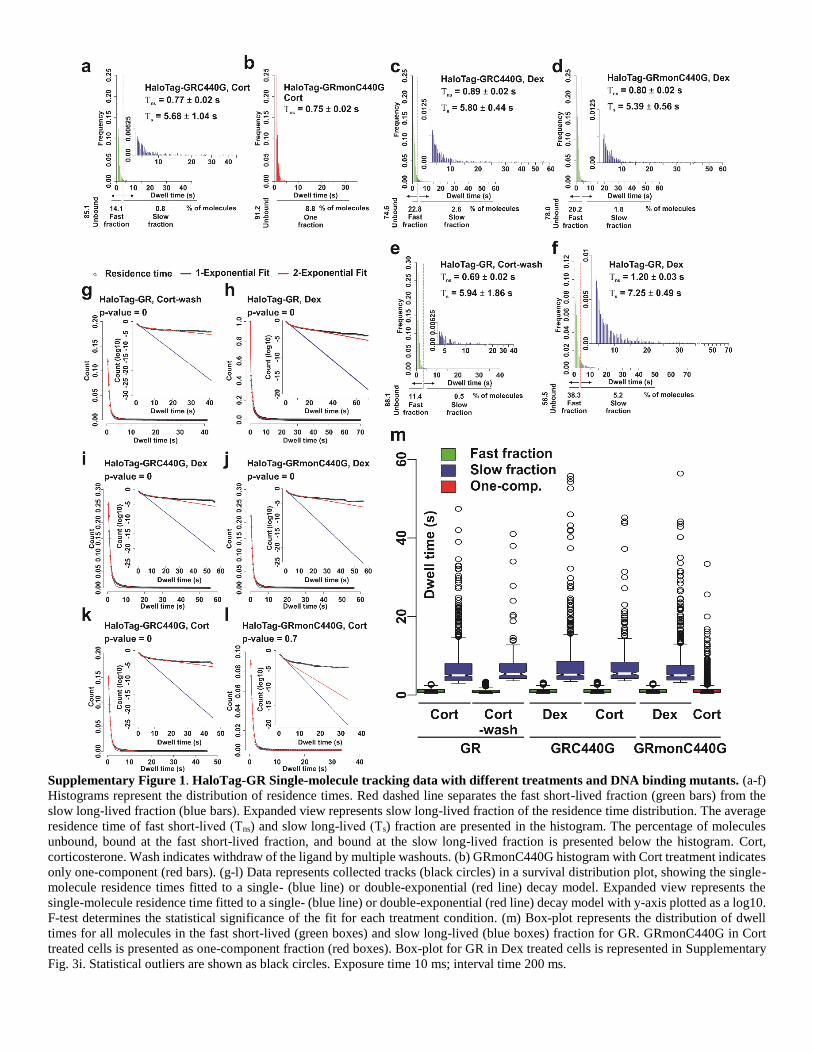
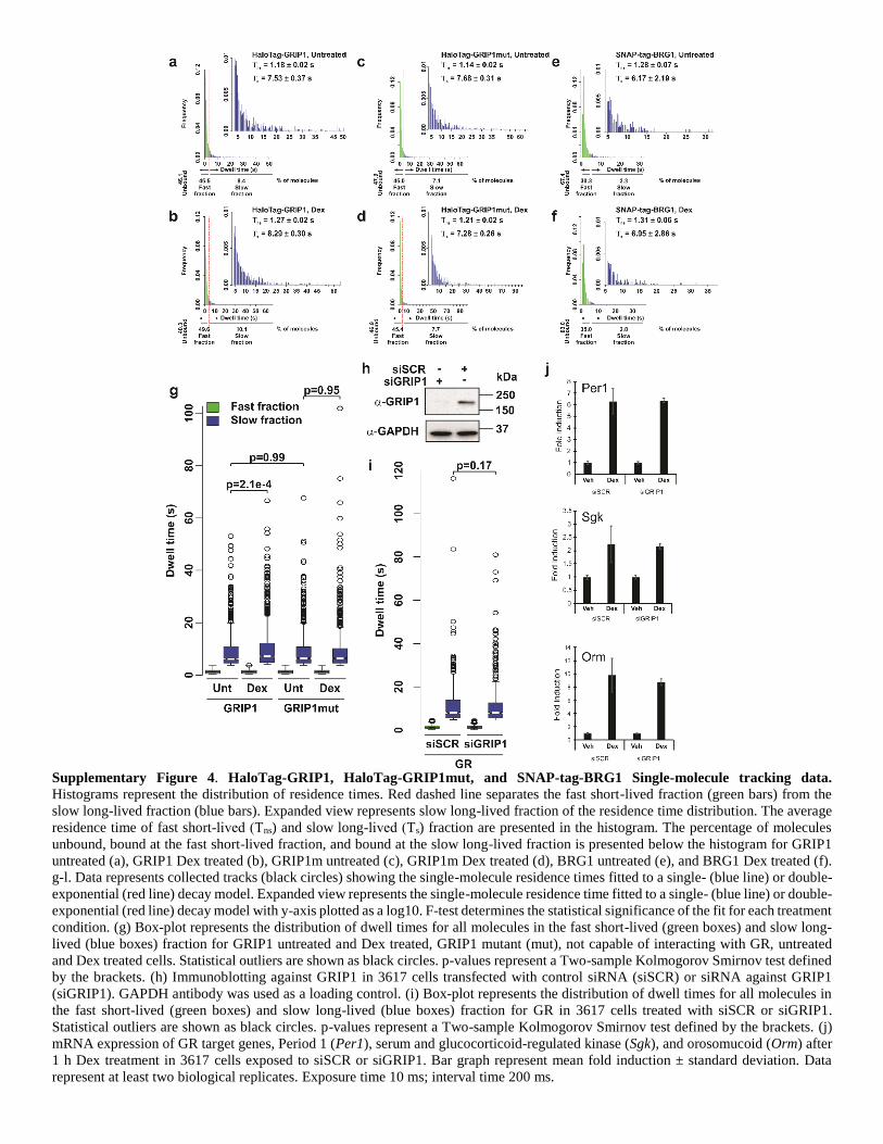
Supplementary Figure 1. HaloTag-GR Single-molecule tracking data with different treatments and DNA binding mutants. (a-f)

Histograms represent the distribution of residence times. Red dashed line separates the fast short-lived fraction (green bars) from the

slow long-lived fraction (blue bars). Expanded view represents slow long-lived fraction of the residence time distribution. The average

residence time of fast short-lived (Τns) and slow long-lived (Τs) fraction are presented in the histogram. The percentage of molecules

unbound, bound at the fast short-lived fraction, and bound at the slow long-lived fraction is presented below the histogram. Cort,

corticosterone. Wash indicates withdraw of the ligand by multiple washouts. (b) GRmonC440G histogram with Cort treatment indicates

only one-component (red bars). (g-l) Data represents collected tracks (black circles) in a survival distribution plot, showing the single-

molecule residence times fitted to a single- (blue line) or double-exponential (red line) decay model. Expanded view represents the

single-molecule residence time fitted to a single- (blue line) or double-exponential (red line) decay model with y-axis plotted as a log10.

F-test determines the statistical significance of the fit for each treatment condition. (m) Box-plot represents the distribution of dwell

times for all molecules in the fast short-lived (green boxes) and slow long-lived (blue boxes) fraction for GR. GRmonC440G in Cort

treated cells is presented as one-component fraction (red boxes). Box-plot for GR in Dex treated cells is represented in Supplementary

Fig. 3i. Statistical outliers are shown as black circles. Exposure time 10 ms; interval time 200 ms.

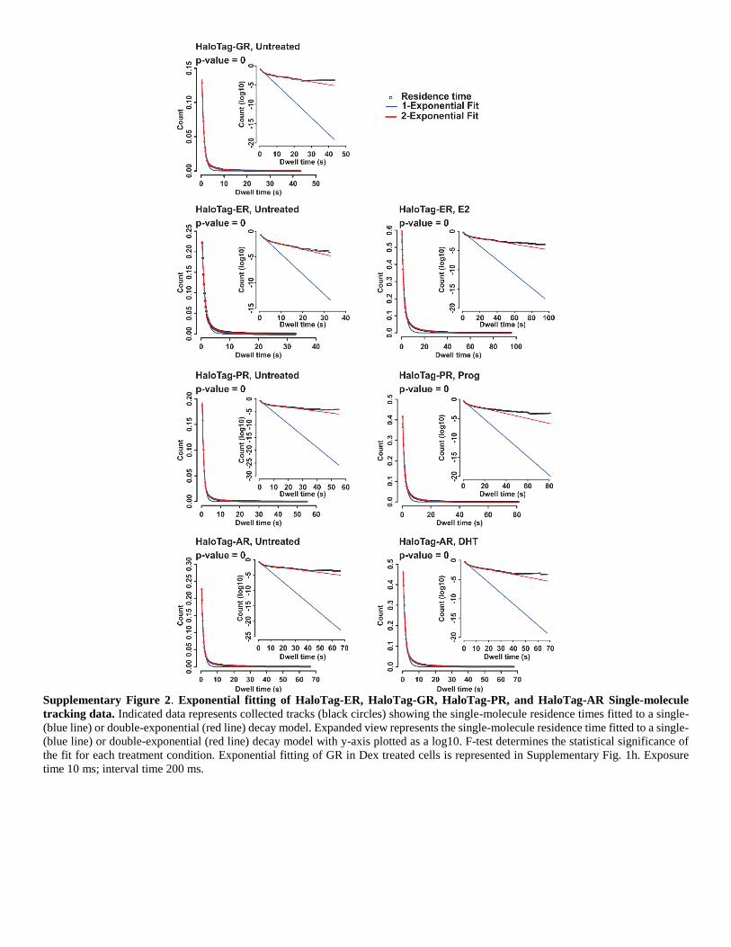
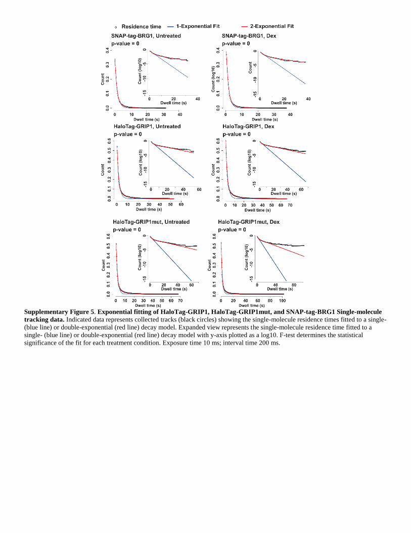
Supplementary Figure 2. Exponential fitting of HaloTag-ER, HaloTag-GR, HaloTag-PR, and HaloTag-AR Single-molecule

tracking data. Indicated data represents collected tracks (black circles) showing the single-molecule residence times fitted to a single-

(blue line) or double-exponential (red line) decay model. Expanded view represents the single-molecule residence time fitted to a single-

(blue line) or double-exponential (red line) decay model with y-axis plotted as a log10. F-test determines the statistical significance of

the fit for each treatment condition. Exponential fitting of GR in Dex treated cells is represented in Supplementary Fig. 1h. Exposure

time 10 ms; interval time 200 ms.

Supplementary Figure 3. HaloTag-ER, HaloTag-GR, HaloTag-PR, and HaloTag-AR Single-molecule tracking data. (a)

Comparison of dwell time distribution between HaloTag alone (red line), steroid receptor (SR) in untreated (black line), and SR in

hormone treated (blue line) cells. Both axes are plotted as a log10. (b-h) Histograms represent the distribution of residence times. Red

dashed line separates the fast short-lived fraction (green bars) from the slow long-lived fraction (blue bars). Expanded view represents

slow long-lived fraction of the residence time distribution. The average residence time of fast short-lived (Τns) and slow long-lived (Τs)

fraction are presented in the histogram. The percentage of molecules unbound, bound at the fast short-lived fraction, and bound at the

slow long-lived fraction is presented below the histogram for ER (b), GR (c), PR (d), and AR (e) untreated, and ER E2 treated (f), PR

Prog treated (g), and AR DHT treated (h). GR Dex treated histogram is represented in Supplementary Fig. 1f. (i) Box-plot represents

the distribution of dwell times for all molecules in the fast short-lived (green boxes) and slow long-lived (blue boxes) fraction for ER

untreated and E2 treated, GR untreated and Dex treated, PR untreated and Prog, AR untreated and DHT treated cells. Statistical outliers

are shown as black circles. p-values represent a Two-sample Kolmogorov Smirnov test defined by the brackets. Exposure time 10 ms;

interval time 200 ms.

Supplementary Figure 4. HaloTag-GRIP1, HaloTag-GRIP1mut, and SNAP-tag-BRG1 Single-molecule tracking data.

Histograms represent the distribution of residence times. Red dashed line separates the fast short-lived fraction (green bars) from the

slow long-lived fraction (blue bars). Expanded view represents slow long-lived fraction of the residence time distribution. The average

residence time of fast short-lived (Τns) and slow long-lived (Τs) fraction are presented in the histogram. The percentage of molecules

unbound, bound at the fast short-lived fraction, and bound at the slow long-lived fraction is presented below the histogram for GRIP1

untreated (a), GRIP1 Dex treated (b), GRIP1m untreated (c), GRIP1m Dex treated (d), BRG1 untreated (e), and BRG1 Dex treated (f).

g-l. Data represents collected tracks (black circles) showing the single-molecule residence times fitted to a single- (blue line) or double-

exponential (red line) decay model. Expanded view represents the single-molecule residence time fitted to a single- (blue line) or double-

exponential (red line) decay model with y-axis plotted as a log10. F-test determines the statistical significance of the fit for each treatment

condition. (g) Box-plot represents the distribution of dwell times for all molecules in the fast short-lived (green boxes) and slow long-

lived (blue boxes) fraction for GRIP1 untreated and Dex treated, GRIP1 mutant (mut), not capable of interacting with GR, untreated

and Dex treated cells. Statistical outliers are shown as black circles. p-values represent a Two-sample Kolmogorov Smirnov test defined

by the brackets. (h) Immunoblotting against GRIP1 in 3617 cells transfected with control siRNA (siSCR) or siRNA against GRIP1

(siGRIP1). GAPDH antibody was used as a loading control. (i) Box-plot represents the distribution of dwell times for all molecules in

the fast short-lived (green boxes) and slow long-lived (blue boxes) fraction for GR in 3617 cells treated with siSCR or siGRIP1.

Statistical outliers are shown as black circles. p-values represent a Two-sample Kolmogorov Smirnov test defined by the brackets. (j)

mRNA expression of GR target genes, Period 1 (Per1), serum and glucocorticoid-regulated kinase (Sgk), and orosomucoid (Orm) after

1 h Dex treatment in 3617 cells exposed to siSCR or siGRIP1. Bar graph represent mean fold induction ± standard deviation. Data

represent at least two biological replicates. Exposure time 10 ms; interval time 200 ms.

Supplementary Figure 5. Exponential fitting of HaloTag-GRIP1, HaloTag-GRIP1mut, and SNAP-tag-BRG1 Single-molecule

tracking data. Indicated data represents collected tracks (black circles) showing the single-molecule residence times fitted to a single-

(blue line) or double-exponential (red line) decay model. Expanded view represents the single-molecule residence time fitted to a

single- (blue line) or double-exponential (red line) decay model with y-axis plotted as a log10. F-test determines the statistical

significance of the fit for each treatment condition. Exposure time 10 ms; interval time 200 ms.

Supplementary Figure 6. HaloTag-c-JUN, HaloTag-c-FOS, and HaloTag-a-FOS Single-molecule tracking. Histograms represent

the distribution of residence times. Red dashed line separates the fast short-lived fraction (green bars) from the slow long-lived fraction

(blue bars). Expanded view represents slow long-lived fraction of the residence time distribution. The average residence time of fast

short-lived (Τns) and slow long-lived (Τs) fraction are presented in the histogram. The percentage of molecules unbound, bound at the

fast short-lived fraction, and bound at the slow long-lived fraction is presented below the histogram for c-JUN untreated (a), c-JUN Dex

treated (b), c-FOS untreated (c), c-FOS Dex treated (d), and a-FOS untreated (e). (f-j) Data represents collected tracks (black circles)

showing the single-molecule residence times fitted to a single- (blue line) or double-exponential (red line) decay model. Expanded view

represents the single-molecule residence time fitted to a single- (blue line) or double-exponential (red line) decay model with y-axis

plotted as a log10. F-test determines the statistical significance of the fit for each treatment condition. (k) Box-plot represents the

distribution of dwell times for all molecules in the fast short-lived (green boxes) and slow long-lived (blue boxes) fraction for c-FOS

untreated and Dex treated, a-FOS untreated, c-JUN untreated and Dex treated cells. Statistical outliers are shown as black circles. p-

values represent a Two-sample Kolmogorov Smirnov test defined by the brackets. Exposure time 10 ms; interval time 200 ms.

Supplementary Figure 7. HaloTag-GR in the presence of GFP, GFP-c-FOS, and GRP-a-FOS Single-molecule tracking data.

Histograms represent the distribution of residence times. Red dashed line separates the fast short-lived fraction (green bars) from the

slow long-lived fraction (blue bars). Expanded view represents slow long-lived fraction of the residence time distribution. The average

residence time of fast short-lived (Τns) and slow long-lived (Τs) fraction are presented in the histogram. The percentage of molecules

unbound, bound at the fast short-lived fraction, and bound at the slow long-lived fraction is presented below the histogram for GR+GFP

Dex treated (a), GR+GFP-c-FOS Dex treated (b), and GR+GFP-a-FOS Dex treated (c). (d-f) Data represents collected tracks (black

circles) showing the single-molecule residence times fitted to a single- (blue line) or double-exponential (red line) decay model.

Expanded view represents the single-molecule residence time fitted to a single- (blue line) or double-exponential (red line) decay model

with y-axis plotted as a log10. F-test determines the statistical significance of the fit for each treatment condition. (g) Box-plot represents

the distribution of dwell times for all molecules in the fast short-lived (green boxes) and slow long-lived (blue boxes) fraction for

GR+GFP Dex treated, GR+GFP-c-FOS Dex treated, and GR+GFP-a-FOS Dex treated cells. Statistical outliers are shown as black

circles. p-values represent a Two-sample Kolmogorov Smirnov test defined by the brackets. (h) Box-plot represents the distribution of

dwell times for all molecules in the fast short-lived (green boxes) and slow long-lived (blue boxes) fraction for GR+GFP-aFOS Dex

treated, GRC440G Dex treated, and GRmonC440G Dex treated cells. Statistical outliers are shown as black circles. p-values represent

a Two-sample Kolmogorov Smirnov test defined by the brackets. Exposure time 10 ms; interval time 200 ms.

Supplementary Figure 8. Full immunoblots shown in Figure 2a and b. (a) (Upper blot) Immunoblotting against GR shown in Figure

2a. (Lower blot) Immunoblotting against GAPDH shown in Figure 2a. (b) (Upper blot) Immunoblotting against GR shown in Figure

2b. (Lower blot) Immunoblotting against GAPDH shown in Figure 2b. MW, molecular weight marker (Bio-Rad Precision Plus Protein

WesternC Standards).

Supplementary Figure 9. Full immunoblots shown in Supplementary Figure 4h. (Upper blot) Immunoblotting against GRIP1 shown

in Supplementary Figure 4h. Non-specific ban indicated with red arrow. (Lower blot) Immunoblotting against GAPDH shown in

Supplementary Figure 4h. MW, molecular weight marker (Bio-Rad Precision Plus Protein WesternC Standards). Full immunoblots also

show dilution of siSCR sample to half (0.5) or to quarter (0.25) of the full sample.

Supplementary Table 1

Photobleaching kinetics

Factor Exposure time (ms)

Interval time (ms)

kB Mean

survival time (s)

Mean number of frames survived

Half-life of molecule (s)

90th Percentile of survival time (s)

90th Percentile of number of frames

survived

HaloTag-GR 10 30 0.077611224 12.88473 429.4911 8.931017 29.66819698 988.9399

HaloTag-GR 10 100 0.05779047 17.30389 173.0389 11.994143 39.84368171 398.4368

HaloTag-GR 10 150 0.037185388 26.89228 179.2819 18.640310 61.92177106 412.8118

HaloTag-GR 10 200 0.026757192 37.37313 186.8656 25.905079 86.05481054 430.2741

HaloTag-GR 10 250 0.021859331 45.74706 182.9882 31.709442 105.33648714 421.3459

HaloTag-GR 10 400 0.013349792 74.90754 187.2688 51.921947 172.48097444 431.2024

HaloTag-GR 10 800 0.006760098 147.92685 184.9086 102.535081 340.61416710 425.7677

HaloTag-GR 10 1000 0.006310875 158.45662 158.4566 109.833762 364.85986087 364.8599

HaloTag-GR 10 1500 0.003385584 295.37003 196.9134 204.734905 680.11463330 453.4098

HaloTag-GR 10 2000 0.001326314 753.96923 376.9846 522.611647 1736.07831434 868.0392

HaloTag-GR 10 2500 0.000983132 1017.15786 406.8631 705.040101 2342.09251992 936.8370

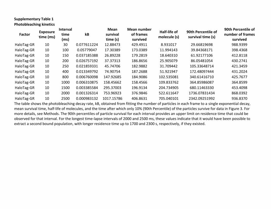
The table shows the photobleaching decay rate, kB, obtained from fitting the number of particles in each frame to a single exponential decay, mean survival time, half-life of molecules, and the time after which only 10% (90th Percentile) of the particles survive for data in Figure 3. For more details, see Methods. The 90th percentiles of particle survival for each interval provides an upper limit on residence time that could be observed for that interval. For the longest time-lapse intervals of 2000 and 2500 ms, these values indicate that it would have been possible to extract a second bound population, with longer residence time up to 1700 and 2300 s, respectively, if they existed.