II III 111111 1111 111111111111 1111 1111 111111 11111111 1111 11111111111 3 1176 00168 7889 I , I I . NASA Technical Memorandum 83123 NASA-TM-8312319810019313 Two-boundary Grid Generation for the Solution of the Three-dimensional Compressible Navier-Stokes Equations B. E. Smith May 1981 NJ\5I\ National Aeronautics and Space Administration Langley Research Center Hampton. Virginia 23665 FOR· REFERENCE -.;: , ............. ," JUN 29 1981 r "" "'" "" ""
Transcript
II III 111111 1111 111111111111 1111 1111 111111 11111111 1111 11111111111
3 1176 00168 7889 I
, I
I .
NASA Technical Memorandum 83123
NASA-TM-8312319810019313
Two-boundary Grid Generation for the Solution of the Three-dimensional Compressible N avier-Stokes Equations
B. E. Smith
May 1981
NJ\5I\ National Aeronautics and Space Administration
Langley Research Center Hampton. Virginia 23665
FOR· REFERENCE -.;: , ............. ,"
JUN 29 1981
L~8i~/t~',', i'~'~12.\
li"\~'~PTryN: \~In~'~\".\
r '''~'''' "" ~ U~ ~1W~' "'" "" ""
LIST OF TABLES . .
LIST OF FIGURES LI ST OF SYMBOLS SUMMARY .... 1. INTRODUCTION. i •
2. ANALYSIS ..
TABLE OF CONTENTS
2.1 Navier-Stokes Equations of Motion.
2.2 Transformed Equations of Motion.
2.3 Definition of a Computational Domain and
Page
. . iii
v ix xv
1
6
7
• • • 10
Transformation Data . . . . 16
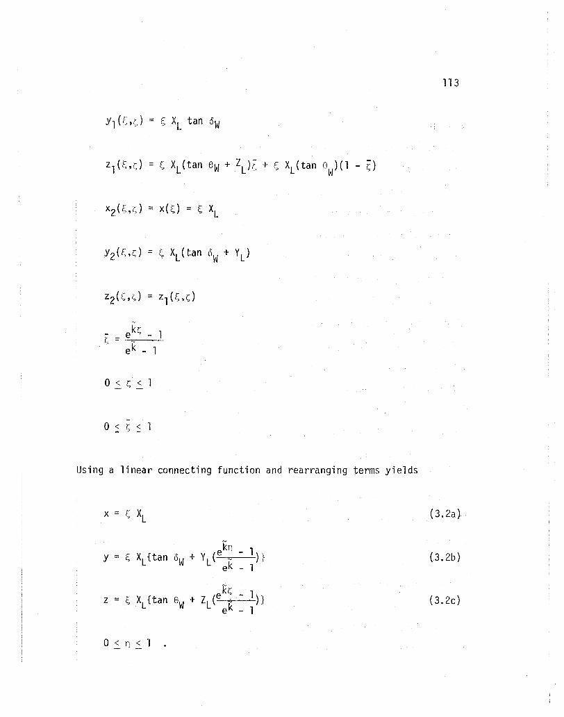
2.4 Two-Boundary Grid Generation . . . . 20
2.4.1 Approximate Boundary-Fitted Coordinate Systems Using Tension Spline Functions . 31
2.4.2 Transformation for a Wedge-Cylinder Corner. . 35
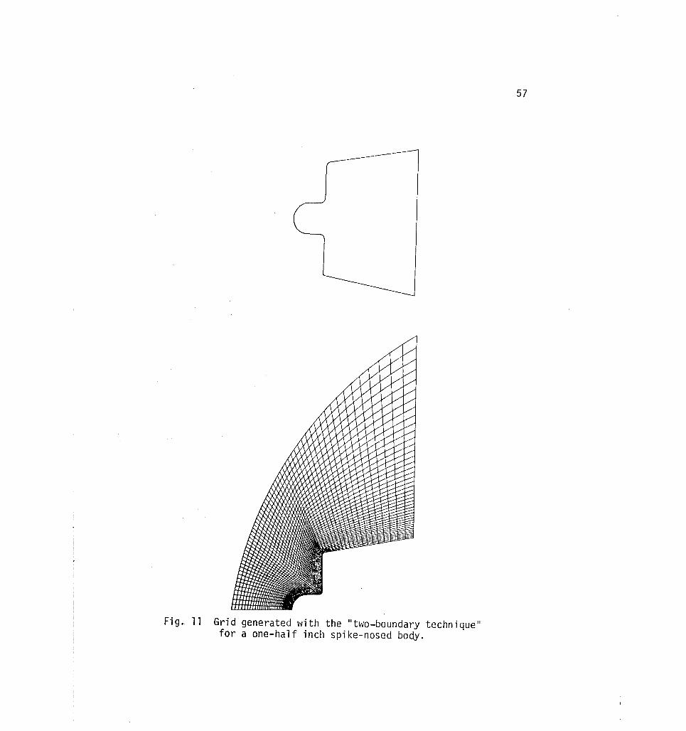
2.4.3 Transformation for a Spike-Nosed Body 48
2.5 Initial and Boundary Conditions ..... 61
2.5.1 Boundary Conditions for Supersonic Flow About Wedge-Cylinder Corners. . . . . . . . . . . 64
2.5.2 Boundary Conditions for Supersonic Flow About Spike-Nosed Bodies 68
51. Comparison of density solution for grid concentration change line = 53 . . . . . .. ...... . . 140
52. Comparison of density solution for outer boundary change 1 ine = 1 ..................... 141
53.
54.
Comparison of density solution for outer boundary change line = 29
Comparison of density solution for outer boundary change line = 53 ....
142
· . 143
viii
Figure
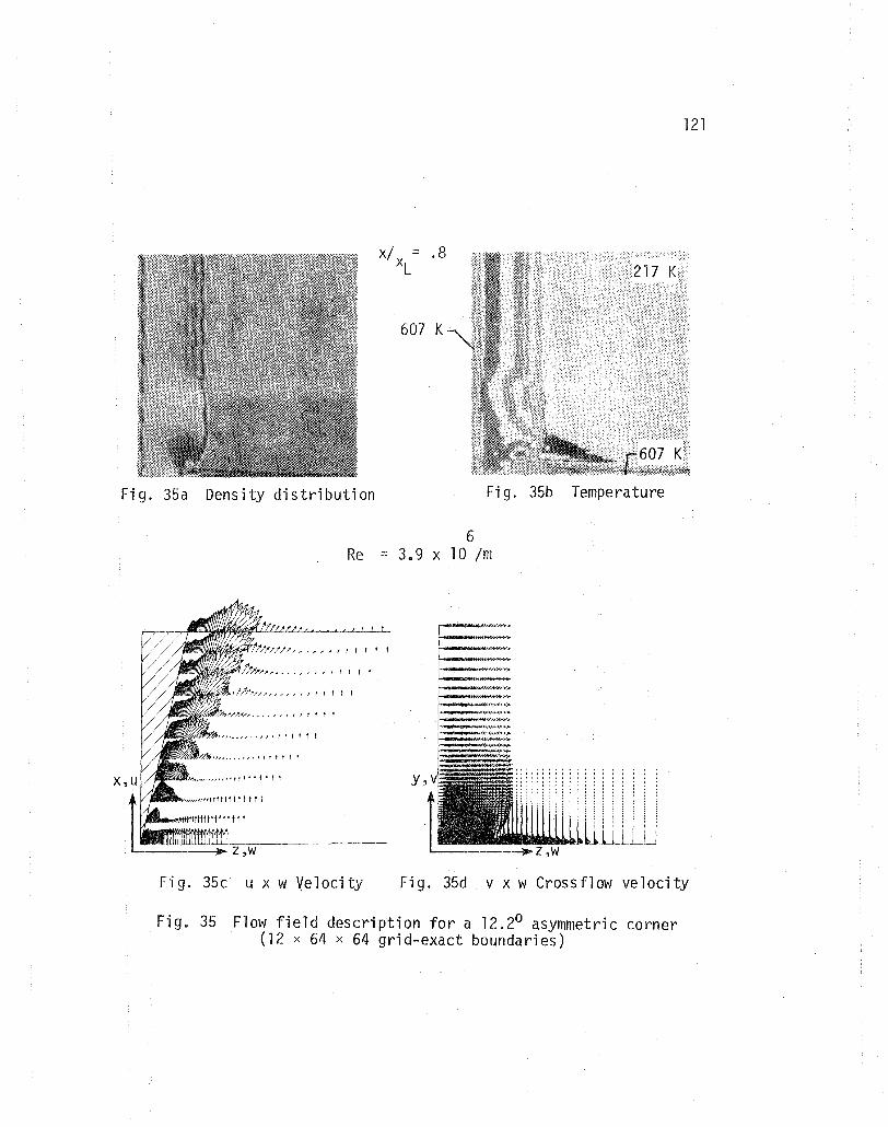
55. Shadowgraphs of an oscillating flow field . . . . . 145
56. Density distribution during one cycle of oscillation for a one and one-half inch spike-nosed body. . . . 147
57. Surface pressure on one and one-half inch spike-nosed body ........ . 148
B
c 00
e
F,G,H
g",h" -+-+.,jo-i ,j ,k
LIST OF SYr1BOLS
parameter governing grid concentration for spike-nosed body grids
intermediate variables used in computing the pressure on a cylinder surface for wedge-cylinder corner meshes
specific heat at constant volume
specific heat at constant pressure
free stream speed of sound
intermediate variables used in computing pressure on a wedge surface for \.,.edge-cyl inder corner meshes
interna 1 energy
vector fluxes for coordinate directions
symbol· for flux vectors in a compact definition of the equations of motion
basis functions for cubic connecting function
second derivatives for tension spline approximation
unit vectors in the physical coordinate system
Jacobian matrix
inverse Jacobian matrix
determinant of inverse Jacobian matrix
magnitude of normal vector on bounding surfaces
coefficient of heat conduction
parameters governing the grid concentration for wedgecyl inder grids
parameters governing the grid concentration for spikenosed body grids
parameter governing the grid concentration for planar intersecting corner grids
ix
-k
L
M
M 00
m,n
N
N p
q
R
R =Re e 00
s
s,t
S
T
parameter governing grid concentration for planar intersecting corner grids
characteristic length
number of points describing the inside boundary for spike-nosed body grids
free stream Mach number
number of points describing boundaries for tension spline approximation
number of points in tension spline approximation
normal direction
pressure
heat conduction vector
components of heat conduct vector
radial direction
cylinder radii for wedge-cylinder grid description
radius of circle describing the outside boundary for spike-nosed body meshes
free stream Reynolds number
parametric variable for an airfoil grid
parametric variables
Sutherland viscosity law constant
four-dimensional array containing state variables and transformation data
temperature
reference temperature for Sutherland viscosity law
time
x
u
u,v,w -u
-v
parametric variable for inner boundary of spike-nosed body meshes
vector of state variables
velocity components in the physical domain
velocity vector
velocity used in computing time step for the finite difference technique
xi
X(),Y(),Z(),} functions relating the computational domain to the x(),y(),z() physical domain
x,y,z
x,y
x,y
-a
y
Yx,Yy'Yz
L'I~,L'ln,L'lZ;:
~t
8
functions relating the computational domain to the physical domain with boundary parameterization and third independent variabl e "connecti ng functi on"
coordinates for the physical domain
symbols for coordinates in the compact definition of the equations of motion
coordinates for the inside boundary of spike-nosed body grids
physical coordinate position in windward direction for the initial solid surface in wedge-cylinder corner grids
physical coordinate in the windward direction for the final grid plane in the wedge-cylinder corner grids
coefficient for pressure damping
ratio of specific heats
directional cosines of the normal vector at a solid wall
constant increments in the computational coordinates
increment in time
angle defining a parametric variable for the outside boundary of spike-nosed grids
angles defining boundaries of wedge cylinder corner grids
p
a
T
c/>X'c/>y'c/>Z
\}Jl,\}J2
Subscripts:
B
W
00
xii
angles defining boundaries of planar intersecting corner grids
intermediate angle for computing pressure boundary condition for wedge-cylinder corner grids
molecular viscosity
reference viscosity in Sutherland viscosity law
bulk viscosity
coordinates in the computational domain
redistributed coordinates relative to the computational domain
density
tension parameter
stress tensor
wedge angle for wedge-cylinder corner grids
angle of rotation for three-dimensional spike-nosed grids
components of viscous dissipation function
intermediate angles for wedge-cylinder grids
boundary value
solid wall value
free stream value
Superscripts:
I
o
Indices:
I,J,K,L
i ,j ,k
Opera tors:
o
a
inside boundary for spike-nosed body grids
outside boundary for spike-nosed body grids
indices used in four-dimensional S array
point indices
boundary indicator
gradient operator
inner product operator
finite difference operators
linear interpolation operator
partial differentiation
xiii
SUMMARY
TWO-BOUNDARY GRID GENERATION FOR THE SOLUTION OF THE THREE-DIMENSIONAL COMPRESSIBLE
NAVIER-STOKES EQUATIONS
Robert Edward Smith
xv
A grid generation technique called the IItwo-boundary technique ll is
developed and applied for the solution of the three-dimensional com
pressible Navier-Stokes equations describing laminar flow. The Navier
Stokes equations are presented relative to a xyz cartesian coordinate
system and are transformed to a ;ns computational coordinate system.
The grid generation technique provides the Jacobian matrix describing
the transformation.
The "two-boundary technique" is based on algebraically defining
two distinct boundaries of a flow domain and joining these boundaries
with a IIconnecting function" which is proposed to be linear or cubic
polynomials. The algebraic boundary representation can be analytical
functions or numerical interpolation functions. Control of the distri
bution of the grid in the physical domain is achieved by embedding "con
trol functions" which redistribute the uniform grid of the computational
domain and concentrate or disperse the grid in the physical domain. The
computer program to solve the Navier-Stokes equations is based on a
MacCormack time-split technique and is specifically designed for the
vector architecture and virtual memory of the CYBER 203 computer. The
program "Navier-Stokes solver" is written in the SL/l language which
allows 32-bit word arithmetic operations and storage. The program can
run with 5 x 10⁴ grid points using only primary memory, and the compu
tational speed is 4 x 10⁻⁵ seconds per grid point per time step.
Using the "two-boundary technique," grids are developed for two
distinctly different flow field problems, and compressible supersonic
laminar flow solutions are obtained using the Navier-Stokes solver.
Grids and solutions are obtained for a family of three-dimensional
corners at Hach number 3.64 and Reynolds numbers 2.92 x 10⁵/m and
3.9 x 10⁶/m. Also, grids are derived for spike-nosed bodies, and solu
tions are obtained at Mach number 3 and Reynolds number 7.87 x 10⁶/m.
Coupled with the Navier-Stokes solver, the "two-boundary technique"
is demonstrated to be viable for grid generation associated with com
puting supersonic laminar flow. The technique is easy to apply and is
applicable to a wide class of geometries. The "two-boundary technique"
can serve as the foundation for generating grids with highly complex
boundaries and yield grid pOint distributions that can capture rapidly
changing variables in a flow field.
xv;
1
1. INTRODUCTION
In recent years, the availability of large scale scientific com-
puter systems has resulted in rapid progress in the field of Computa
tional Fluid Dynamics. There is now the capability to calculate many
complex unsteady two-dimensional and steady three-dimensional flows.
MacCormack and Lomax [1]* summarize the "state of the art" for the
computation of compressible viscous fluid flow. For a heat conducting
compressible fluid acting near body surfaces with large separation
regions or inviscid-viscid interactions, the numerical solution of the
Navier-Stokes equations is the preferred approach [1]. An emerging
problem, however, i~ the generation of grid systems on which solutions
can be obtained when there are complex boundary geometries. This prob
lem is compounded in three dimensions. This study addresses the solu
tion of the three-dimensional compressible Navier-Stokes equations,
the generation of grids, and the solution algorithm-computer relation
ship. The emphasis is placed on grid generation.
An algebraic grid generation technique applicable to the Navier
Stokes equations is developed, and a three-dimensional Navier-Stokes
solver (compressible laminar flow) based on a proven numerical tech
nique (MacCormack time-split algorithm [1-4]) is developed for the CDC
CYBER 203 vector computer [5]. Also, flow visualization techniques have
been developed in conjunction with this research but will not be dis
cussed in detail. In order to evaluate the overall system for computing
viscous compressible flow, and in particular the grid generation *The numbers in brackets indicate references.
technique, grids are determined for a family of three-dimensional
corners and two spi ke-nosed bodi es ..
2
The gri d generation technique is called the "two-boundary tech
nique." It is applicable in two and three dimensions and is a method
ology for direct computation of the physical grid as a function of a
uniform rectangular computational grid. The Jacobian matrix of the
transformation can be obtained by direct analytic differentiation. This
is in contrast to the indirect approach where an elliptic partial dif
ferential equation system is solved for the coordinates of the physical
grid relative to the computational grid, and in which the Jacobian
matrix must be obtained by numerical differentiation. The indirect
approach is popularly known as the ITH4method" [1,6-10]. In the
"two-boundary technique, II two separate non-intersecting boundaries are
defined by means of algebraic functions or numerical interpolation
functions. These functions have as independent variables, coordinates
which are normalized to unity. Another function with an independent
variable defined on the unit interval connects the boundaries.
The "two-boundary technique" is based upon concepts found in the
theory of surface definition [11,12]. Gordon and Hall [13] postulate
the essentials of the technique and emphasize finite element grids.
Also, Eiseman [14-16] uses a form of the technique in generating grids
for multiconnected two-dimensional domains. In this investigation the
"two-boundary technique" is developed and is analyzed for finite differ
ence solutions for fluid flow applications. Low order polynomials
(linear and cubic) are used for connecting functions. For the cubic
3
connecting function, orthogonality can be enforced at the boundaries
through knowledge of the normal derivatives there. Control of the grid
(grid spacing in the physical domain) is achieved by the superposition
onto the independent variables algebraic or transcendental functions
with desirable characteristics. Splines under tension [17-19J are pro
posed for approximate boundary defi nition. The II two-boundary techni que"
is used to algebraically generate grids for a family of three-dimensional
corners and to generate a combined algebraic-numeric grid for spike
nosed bodies. The derivatives composing the Jacobian matrix for the
three-dimensional corners and spike-nosed bodies are presented for
obtaining numerical solutions of the Navier Stokes equations.
The CDC CYBER 203 is a large scale computer with vector processing
architecture and virtual memory. Generally efficiency using a vector
computer increases with increasing vector length, however, considerable
attention must be given to the algorithm-machine architecture relation
and balancing the vector length with practical limits of primary memory.
A MacCormack time-split solution algorithm is programmed for the
CYBER 203 computer and is called the "Navier-Stokes solver." The
MacCormack technique is used because of its robustness and adaptability
to vector processing. Another primary consideration when developing a
"Navier-Stokes solver" on a large complex computer is the capability to
solve a wide class of problems with a minimum of programming changes.
This has been accomplished by programming the complete transformed
equations of motion and storing all nine elements of the Jacobian
matrix of the transformation at each grid point (transformation data).
4
Supplying the transformation data from a grid generation technique and
programming the boundary conditions "for a given problem (separate sub
routine) allows the program be applied to virtually any laminar fluid
flow problem. Since the split MacCormack technique is used, two
dimensional solutions can be obtained without unnecessary computations.
The operator for the third dimension is bypassed. A final important
point relative to the Navier-Stokes solver is that the MacCormack tech
nique is written in the SL/l language [20J and uses the 32-bit arithmetic
option of the CYBER 203. By using 32-bit words, twice the in-core stor
age is available and approximately twice the computational speed is
achieved compared to the use of normal 64-bit words. There are approxi
mately two million words of primary memory and the computational speed
is 4 x 10⁻⁵ seconds per grid point per time step for the 32-bit word
length. For the explicit technique, no significant degeneration in
accuracy is observed using the smaller word size. The Navier-Stokes
solver is independent of the grid generation technique, and the trans
formation data from any technique can be used by the code.
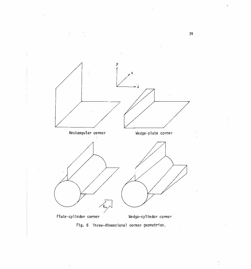
Using the IItwo-boundary technique ll grids are developed for two
distinctly different flow field problems, and compressible supersonic
laminar flow solutions are obtained using the computer program based on
the MacCormack technique. A set of algebraic grid generation equations
are developed using the IItwo-boundary technique ll for a family of three
dimensional corners consisting of wedge-cylinder, plate-cylinder,
approximate wedge-plate, and approximate rectangular corners. It is
also shown that exact grids for planar intersecting corners can be
5
derived with the "two-boundary technique." Corner flow solutions are
obtained on a 20 x 36 x 36 grid and a 12 x 64 x 64 grid. The solutions
obtained on the 12 x 64 x 64 grid are compared with physical experiments
and other numerical experiments. The Mach number used is 3.64 and the
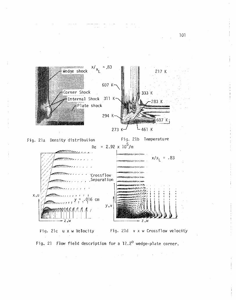
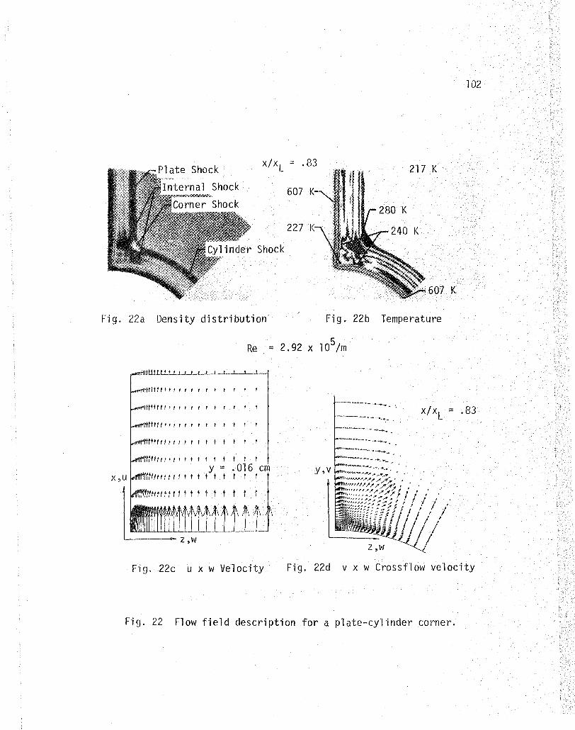
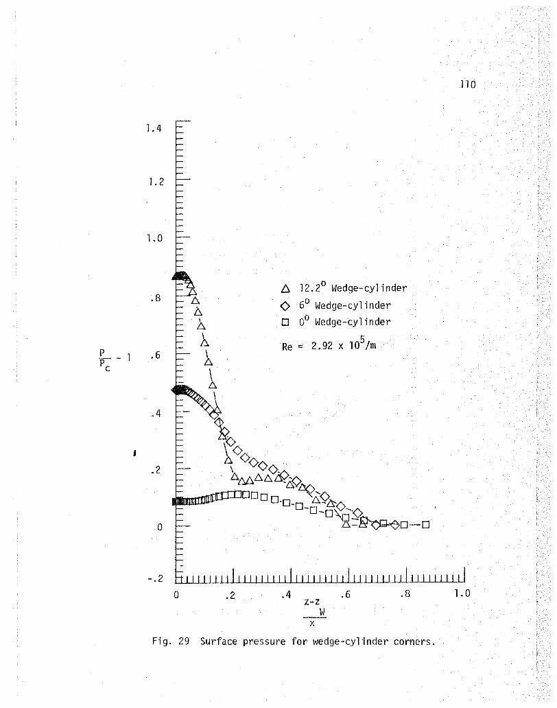
Reynolds number is 2.92 x 10⁵/m and 3.9 x 10⁶/m.
Also, algebraic grids are derived using the "two-boundary technique"
for spike-nosed bodies. In particular, grids for a one-half inch spike
nosed body and a one and one-half inch spike-nosed body are obtained.
Supersonic flow solutions at Mach number 3 and Reynolds number
7.87 x 10⁶/m are obtained about these configurations. Unlike the flows
about the three-dimensional corners, the flow about the spike-nosed
bodies is unsteady. The amplitude of the oscillations about the one-half
inch nose body is quite small, however, the one and one-half inch spike
nosed body flow field oscillates with a large amplitude. The high
amplitude solutions are compared with physical experiments. The flow
fields are two-dimensional axisymmetric, but are solved with a three
dimensional Navier-Stokes solver resulting in considerable savings of
development time for a specialized axisymmetric code.
For flow visualization. a relatively novel approach has been
developed where a color spectrum is used to display a scalar variable
such as density, Mach number, etc •• on a two-dimensional slice of a flow
field. Sequences of pictures can show the history of a developing flow
or a scan of the flow field in a three-dimensional domain. The Diccomed
Digital Display/Film Writer system which is normally used for environ
mental image processing is used for the flow visualization.
6
In summary, the main objectives of this study are the development
of an algebraic grid generation procedure, the development of software
to solve the compressible three-dimensional Navier-Stokes equations on
a vector computer using the results of the grid generation technique,
and the application of the grid generation technique and software to
solve specific supersonic flow problems. The organization is as
follows. In Chapter 2 the three dimensional compressible Navier-Stokes
equations are presented relative to a Cartesian coordinate system and
are transformed to a uniform grid computational coordinate system.
This introduces the information that must be determined by the grid
generation technique. The "two-boundary technique" is developed and
applied to generate grids and Jacobian derivatives for a family of
three-dimensional corners, spike-nosed bodies, and an airfoil configura
tion. In Chapter 3, the MacCormack technique is presented, and its
compatibility with the CYBER 203 is described. In Chapter 4, supersonic
flow solutions about three-dimensional corners and spike-nosed bodies
obtai ned with the "two-boundary technique" and Navi er-Stokes solver
are described.
2. ANALYSIS
This chapter develops the equations of motion and the "two
boundary technique" for grid generation. Grids and boundary conditions
are developed for a family of three-dimensional corners and for spike
nosed bodies. Also, grids are developed for airfoil boundaries using
splines under tension.
7
2.1 Navier-Stokes Equations of Motion
The governing equations which describe the motion of a viscous
compressible heat conducting fluid are the continuity equation, momen
tum equations, and energy equation. These'equations are derived from
the concept of continuum mechanics. The continuum concept and deriva
tion of the Navier-Stokes equations of motion are found in several
references, of which Schlichting [21] is the most notable.
Expressed in symboic form the Navier-Stokes equations of motion
are:
Continuity: .£Q. + 'V at . (pUJ = 0, (2.1a)
Momentum: a(pu) + 'V • (puu at - T) = 0, (2.1b)
Energy: a(pe) + 'V • (peu + q - U • T) 0. (2.1c) at =
The stress tensor, dissipation function, and heat conduction for a
rectangular cartesian coordinate system are:
TXX Txy TXZ
T = Txy Tyy Tyz - stress tensor
TXZ Tyz TZZ
where
T = _p + 21I~ + (.' 2) (au + av + aw) xx ax liB - Jll ax ay dZ'
.. " ~
and
T = _p + 211 aV + (llQ _ Jll2 ) (E.!! + av + aWl yy ay I-' ax ay az
_ (au + av) T xy - II ay ax'
_ (aw + au) TXZ - II ax az'
_ (av + aWl Tyz - II az ay'
<P = X
U . T = <P = y
<P = Z
-aT q = -K-x ax
. -aT q = q = -K-y ay
-aT q= -K-z az
UTxx + VTxy + WTXZ
UT + VT + WT xy yy yz - dissipation
UTXZ + VTyz + WTZZ
- Heat flux vector,
8
function,
9
The viscosity coefficient ~ is a function of temperature and is
adequately approximated by Sutherland's semiempirical equation:
with
The bulk viscosity coefficient ~S is set equal to zero. This is
a reasonable assumption for a monatomic gas where the molecules has no
internal degree of freedom. For a polyatomic gas the bulk viscosity is
not always zero and can be the same order of magnitude as the molecular
viscosity in sound propagation and shock structure. A detailed discus
sion of bulk viscosity is given by Vincenti and Kruger [22].
At this point there are five coupled partial differential equations
and one algebraic equation with eight .unknowns: p, u, v, w, P, e,
T, and ~. In order to have a complete system, there must be two addi
tional equations relating the unknowns. The equation of state is
P = P (p,T),
and for a perfect gas P = pRT and e = CVT where Cv is the specific
heat at constant volumn, and R is the gas constant. For compatible
boundary conditions this system of equations is solvable.
10
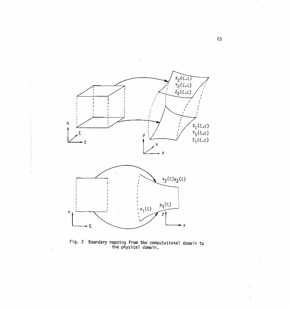
2.2 Transformed Equations of Motion
The equations of motion in Section 2.1 are expressed in terms of a
Cartesian coordinate system. If an object is defined in this coordinate
system and a flow is to take place about the object, it is desirable to
perform the computation in a coordinate system which conforms to the
boundaries of the object. There are two primary reasons for wanting the
coordinate system to be boundary-fitted. Boundary-fitted coordinates
afford the ability to apply boundary conditions exactly avoiding inter
polation error, and they minimize the logic that is necessary to apply
boundary conditions. The penalty for these advantages is added com
plexity of the equations of motion. Another consideration is that when
the domain of the flow field is discretized, it is desirable to have
grid points concentrated in certain regions where high rates of change
are likely to occur. For instance, in the boundary layer region more
grid points are necessary to resolve the rapid change in the state
variables. If the cartesian coordinate system where the object is
defined is called the physical domain, the coordinate system relative
to the boundaries of the object is called the computational domain. The
relationship between the physical domain and the computational domain is
a unique single-valued transformation with continuous derivatives such
that if the coordinates in the computational domain are ~, n, ~:
then
~ = ~(x,y,z), n = n(x,y,z), and ~ = ~(x,y,z).
11
Conversely,
where x, y, and z are coordinates in the physical domain. Since
the equations of motion in terms of the Cartesian coordinate system of
the physical domain are advantageously solved in terms of the coordinate
system of the computational domain, the equations must be transformed.
This is accomplished by expressing the derivatives of the state variables
with respect to the xyz components of the physical domain in terms of
the ~ns components of the computational domain as follows:
au ax
av ax
aw ax
au ay
av ay
av az
aw az
=
au a~
av ~
au an
av an
aw an
aw ~
Notice that u, v, and ware the velocities along the x, y,
and z axes in the physical domain.
-.
,(~e xe lle Xe je Xe ~e Ae lle Ae he ""5€ + Ae 1l€ + Ae ~ + ne ""5€ + ne LLe + je Ae) rt = AX~ ne je
\
, (~e Ze lle Ze je ze \ Me 3€ + Me LLe + Me ~ +
~e A'e "e A'e ,e A'e ~e xe "e xe ,e xe) Ae "3€ + Ae lle + Ae ~ + ne 3€ + ne lle + ne ~ rt £/2
(~.!:!l "e ze 'e.!:!l \ rtz d- _ zz, Me ~e ~ Me lle + Me je I + -/
, (~e ze lle ze je ze Me "3€ + Me lle + Me ~ +
~e Ae lle Ae je Ae ~e xe lle xe je xe) Ae "3€+Ae LLe+he ~+ne 3€+ne LLe+ne ~ rt £/2
(~e Ae lle Ae je Ae) AA Ae "3e + Ae lle + J\e je rt2 + d - = ~
I
, (~e ze "e ze ze ze Me ]e + Me TIe + Me 3e +
~e Ae lle Ae je Ae ~e xe lle xe je . xe\ J\e 1e + he LLe + he 3e + ne "3€ + ne Ue + ne je J rt £/2 -
(~e ~ lle ~ je xe) rt __ xx~ \ne ~e + ne lle + ne je 2 + d -
:sawoJaq ~osual ssa~ls a4l saLqe~~eA paw~oJsue~l a4l JO sw~al UI
2L
ze te xe "5e 3€ 3€
I~ te xe ~osua+ ~ap~o puoJas a4I r = lie lie lie -
Figure 57.- Surface pressure on one and one-half inch spike-nosed body_
3
+::> OJ
149
with Reynolds numbers up to 7.78 x 10⁶jm. Overall, the solutions that
have been obtained simulate the observed phenomena very well.
5. CONCLUS IONS
An algebraic grid generation technique has been developed and
explored in conjunction with the solution of the compressible three
dimensional Navier-Stokes equations. The technique called the "two
boundary technique" is simple to understand, easy to apply, and has a
high degree of generality for the finite difference solution of complex
flow field problems. The "two-boundary technique" allows direct control
of a grid and direct computation of the Jacobian derivatives.
The viability of the grid generation technique is demonstrated
through the development and application of a Navier-Stokes solver which
operates on the CDC CYBER-203 vector computer. The computer program is
based on a MacCormack time-split technique which is chosen because of
its compatibility with vector computer architecture. The finite differ
ence algorithm is written in the SLjl programming language, and the
32-bit word length arithmetic and storage option is used. This option
doubles the number of grid points that can be used for a given amount
of memory and approximately doubles the computational rate as compared
to the normal 64-bit words. Using SLjl and the halfword option the
computational rate is 4 x 10⁻⁵ seconds per grid point per time step,
and solutions with 5 x 10⁴ grid points can be obtained without using
secondary memory. It is concluded from the numerical experiments
presented in the present study that the 32-bit word length is adequate
150
when solving the Navier-Stokes equations for supersonic laminar flow
using an explicit MacCormack technique.
Complex supersonic flow field solutions are obtained for two dis
tinctly different geometries using the IItwo-boundary technique ll for
grid generation and the Navier-Stokes solver. First, supersonic flow
solutions about a family of three-dimensional corners are obtained . . ,
These flow fields reach a steady state but are characterized by strong
shocks and three-dimensional separation. The Mach number is 3.64,
Reynolds numbers are 2.72 x 10⁵/m and 3.9 x 10⁶/m, and the fluid proper
ties are for air. It is shown that the solutions obtained agree well
with physical experiments and other numerical experiments. Also,
corner flow solutions with 5 x 10⁴ grid points are among the most
refined Navier-Stokes solutions obtained to date. The second flow
situation is supersonic flow about spike-nosed bodies. In this case,
the flow is axisymmetric, unsteady, and characterized by a strong bow
shock and massive separation. The Mach number is 3 and the Renolds
number is 7.78 x 10⁶/m• The numerical solutions show dramatically the
oscillating flow generated by the interaction of the bow shock and
shoulder wall of the body. The surface pressure and oscillation fre-
quency compare very well with corresponding wind tunnel experiments.
The successful numerical solution of the flow fields support the primary
conclusion that the IItwo-boundary technique ll is viable for generating
grids for complex flow field solutions. Also, for the spike-nosed
bodies, considerable development time for a specialized axisymmetric
code is saved.
151
Plans for the use of the "two-boundary technique" include develop
ment of grids with wing-fuselage boundaries, analysis of non-orthogonal
grids, development of additional spike-nosed body grids, and the
development of numerical grid control functions.
152
REFERENCES
1. MacCormack, R. W.; and Lomax, H.: "Numerical Solution of Compressible Viscous Flows." Annual Review Fluid Mechanics, 1979, Vol. 11, pp. 238-316, Annual Reviews, Inc.
2. HacCormack, R. W.; and Paullay, A. J.: "Computationa1 Efficiency Achieved by Time Splitting of Finite Difference Operators. II AIAA paper 72-154, Jan. 1972~
3. Shang, J. S.; and Hankey, W. L.: "Numerica1 Solution of the Navier-Stokes Equations for a Three-Dimensional Corner." AIAA paper 77-169, Los Angeles, CA, also AIAA Journal, Vol. 15, Nov. 1977, pp. 1575-82.
4. Shang, J. S.; Hankey, W. L.; and Petty, J. S.: "Three-Dimensional Supersonic Interacting Turbulent Flow Along a Corner." AIAA 78-1210, Seattle, WA, July 1978.
5. Control Data Corporation: "Contro1 Data CYBER-200 Model 203 Computer Hardware Reference Manua1." Publication Number 60256010, Hay 1979.
6. Thompson, J. F.; Thames, F. C.; and Mastin, C. W.: "Automatic Numerical Generation of Body-Fitted Curvilinear Coordinate Systems for Fields Containing Any Number of Arbitrary TwoDimensional Bodies." Journal of Computational Physics, Vol. 15, July 1974, pp. 299-319.
7. Thames, F. C.; Thompson, J. F.; Mastin, C. W.; and Walker, R. L.: "Numerical Solutions for Viscous and Potential Flow About Arbitrary Two-Dimensional Bodies Using Body-Fitted Coordinate Systems. II Journal of Computational Physics, Vol. 24, 245, July 1977, pp. 245-273.
8. Thompson, J. F.; Thames, F. C.; and Shanks, S. P.: "Use of Numeri ca lly Generated Body-Fitted Coordi nate Sys terns for Sol utions of the Navier-Stokes Equations." Proceeding of AIAA 2nd Computer Fluid Dynamics Conference, Hartford, CT, July 1975.
9. Thompson, J. F.; Thames, F. C.; and Mastin, C. W.: "BoundaryFitted Curvilinear Coordinate Systems for Solution of Partial Differential Equations on Field Containing Any Number of Arbitrary Two-Dimensional Bodies." NASA CR-2739, July 1977.
10. Mastin, C. W.; and Thompson, J. F.:- "Elliptic Systems and Numerical Transformations. II Journal of Mathematical Analysi~ and Applications, Vol. 62, Jan. 1978, pp.152-62.
153
11. Coon, S. A.: "Surfaces for Computer-Aided Design of Space Forms." MAC TR-41 (Contract No. AF-33.( 6000-42859) MIT, June 1967. Available from DOC as AD 663504.
12. Gordon, W. J.: "Free-Form Surface Interpolation Through Curved Networks. II General Motors Research Report (GMR 921), Sept. 1969.
13. Gordon, W. J.; and Hall, C.: "Construction of Curvilinear Coordinate Systems and Applications to Mesh Generation." International Journal for Numerical Methods In Engineerin[, Vol. 7, July 1973, pp. 46l-4iT. -
14. Eiseman, P. R.: "Three-Dimensiona1 Coordinates About Wings." Proceeding of the AIAA 4th Computer Fluid Dynamic Conference, Williamsburg, VA, July 1979.
15. Eiseman, P. R.: "A Multi-Surface r~ethod of Coordinate Generation. II
Journal of Computational Physics, Vol. 33, Oct. 1979, pp. 118-150.
16. Eiseman, P. R.: "Geometric Methods in Computational Fluid Dynami cs. II ICASE Report 80-11, April 1980.
17. Schwiekert, D.: "An Interpolation Curve Using Splines in Tension." Journal of Mathematics and Physics, Vol. 45, Sept. 1966, pp.312-317.
18. Cline, A. K.: "Scal er- and Planar-Valued Curve Fitting Using Splines Under Tension." Communications of the ACM, Vol .. 17, No.4, April 1974, pp. 218-233. - -- -- .
19. Pruess, S.: "Properties of Splines in Tension." Journal of Approximation Theory, Vol. 17, Aug. 1970, pp. 86-96.
20. SL/l Reference Manual, Analysis and Computation Division, NASA Langley Research Center, Hampton, VA.
22. Vincenti, W. G.; Kruger, C. H.: Introduction to Physical Gas Dynamics, John Wiley & Son, Inc., 1965.
23. Smith, R. E.; and Weigel, B. L.: "Ana1ytic and Approximate Boundary Fitted Coordinate Systems for Fluid Flow Similation." AlAA Paper 80-0192, Pasadena, CA, Jan. 1980.
24. Dagundji, J.: Topology, Allyn and Bacon, 1968.
25. Ahlberg, J. H.; Nilson, E. N.; and Walsh, S. L.: The Theory of Splines and Their Applications, Academic Press, Inc., 1967.
26. MacCormack, R. W.: liThe Effect of Viscosity in Hypervelocity Impact Crateri ng. II AIM Paper 69-354, May 1969.
27. Roach, P. J.: IIComputational Fluid Dynamics. 1I Hermosa Pub 1 i shers, 1972.
154
28. Holst, T. L.: IINumerical Solution of Axisymmetric Boattail Flow Fields with Plume Simulators. II AIAA Paper 77-224, Jan. 1977.
29. MacCormack, R. W.: IIAn Efficient Numerical Method for Solving the Time-Dependent Compressible Navier-Stokes Equations at High Reynolds Number.1I Computing in Applied Mechanics, ADM, Vol. 18, New York Society of Mechanical Engineering, June 1973.
30. Shang, J. S.: IIImplicit-Explicit Method for Solving the NavierStokes Equations. 1I AIM Journal, Vol. 16, No.5, May 1978, pp. 495-502. --
31. MacCormack, R. W.; and Baldiwn, B. S.: IIA Numerical Method for Solving the Navier-Stokes Equations with Application to Shock Boundary Layer Interactions. 1I AIAA Paper 75-1, Jan. 1975.
32. Smith, R. L; and Pitts, J. I.: liThe Solution of the ThreeDimensional Compressible Navier-Stokes Equations on a Vector Computer. II Third IMAC International Symposium on Computer Methods for Partial Differential Equations, Lehigh University, PA, June 1979.
33. Lambiotte, J. J.: IIEffects of Virtual Memory on Efficient Solution of Two Model Problems. 1I NASA TM X-35l2, July 1977.
34. Charwat, A. F.; and Redekopp, L. G.: IISupersonic Interference Flow Along the Corner of Intersecting Wedges. 1I Men. RM-4863-PR (Contract No. AF49(638)-1700), RAND Corp., July 1966.
35. Stainback, P. C.: IIAn Experimental Investigation at a Mach Number of 4.95 of Flow in the Vicinity of a 900 Interior Corner Alined with the Free-Stream Velocity.1I NASA TN D-184, Feb. 1960.
36. Stainback, P. C.: "Heat-Transfer Measurements at a Mach Number of 8 in the Vicinity of a 900 Interior Corner Alined with the Free-Stream Velocity. II NASA TN D-2417, Aug. 1964.
37. Watson, R. D.: IIExperimental Study of Sharp- and Blunt-Nose Streamwise Corners at Mach 20. 11 NASA TN D-7398, April 1974.
38. Cooper, J. R.; and Hankey, W. L.: "Flow Field Measurements in an Asymmetric Axial Corner at M = 12.5. 11 AIAA Journal, Vol. 12, Oct. 1974, pp. 1353-1357.
155
39. Kulter, P.: "Numerica1 Solution for the Inviscid Supersonic Flow in the Corner Formed by Two I.ntersecti ng Wedges. II AIM Paper 73-675, Palm Springs, CA, July 1973.
40. Shankar, V.; Anderson, D.; and Kulter, P.: "Numerical Solutions for Supersonic Corner Flow. II Journal of Computational Physics, Vol. 17, Oct. 1975, pp. 160-180.
42. Wei nberg, B.; and Rubi n, S.: "Compress i on Corner Flow. II Journal of Fluid Mechanics, Vol. 56, Part 4, May 1975, pp. 753-774.
43. Ghia, K.; and Davis, R.: i'A Study Compres~;ib1e Potential and Asymptotic Viscous Flows for Corner Regions." AIAA Journal, Vol. 12, March 1974, pp. 355-359.
44. Hung, C.; and MacCormack, R.: "Numerica1 Solution of Supersonic Laminar Flow Over a Three-Dimensional Compression Corner." AIAA Paper 77-694, June 1977.
45. Hung, C.; and MacCormack, R.: "Numerica1 Solution of ThreeDimensional Shock Wave and Turbulent Boundary Layer Interactions." AIAA Journal, Vol. 16, Oct. 1978, pp. 1090-1096.
46. Horstman, C.; and Hung, C.: "Computation of Three-Dimensional Turbulent Separated Flows at Supersonic Speeds." AIAA Paper 79-0002, Jan. 1979.
47. Smith, R. L: "Numerica1 Solutions of the Navier-Stokes Equations for a Family of Three-Dimensional Corner Geometries. II AIAA Paper 80-1349, July 1980.
48. Korkegi, R.: liOn the Structure of Three-Dimensional Shock-Induced Separated Flow Regions." AIAA Journal, Vol. 14, No.5, May 1976, pp. 597-600. --
49. Rockwell, D.; and Nandascher, E.: "Se1f-Sustained Oscillations of Impinging Free Shear Layers. II Annual Review of Fluid Mechanics, Vol. II, 1979, pp. 67-94, Annual Review, Inc.--, Palo Alto, CA.
50. Shang, J. S.; Hankey, W. L.; and Smith, R. L: "Flow Oscillations of Spike-Tipped Bodies." AIAA Paper 80-0068, Jan. 1980.
156
51. Butz, J. S.: "Hypersonic Aircraft Will Face Technical Cost Problems. II Aviation Week Including Space Technology, Vol. 70, No. 25, June 1959, pp. 156-169.
52. Harney, D. J.: "Oscillating Shocks on Spike Nose Tips at Mach 3." AFFDL-TM-79-9-FX, Air Force Flight Dynamics Laboratory, WRAFB, Ohi 0, 1979.
53. Widhopf, G. F.; and Voctoria, K. J.: "Numerical Solution of the Unsteady Navier-Stokes Equations for the Oscillatory Flow Over a Concave Body. II Lecture Notes in Physics, No. 35, June 1974, Springler-Verlag, pp. 431-444.
Two-Boundary Grid Generation for the Solution of ~_M_a~y~1_9-8-1--------~ the Three-Dimensional Compressible Navier-Stokes 6. Performing Organization Cod" I Equations I
7. Author(s) 8. Performing Organizdtion Report No. ! R. E. Smith
...------------------------------1 10_ Work Unit No. -, I 9. Performing Organization Name and Address
NASA Langley Research Center Hampton, VA 23665
1 I- Contract or Grant No.
~--~---------------------,-----~ 13. Ty~~ Repon~dP~~dCov~~ 12. Sponsoring A~r>cy Name and Address
National Aeronautics and Space Administration Washington, DC 20546
15. Supplementary Notes
Technical Memorandum 14_ Sponsoring Agency Code
This report is a dissertation submitted to Old Dominion University for partial fulfillment of the requirements for the Degree of Doctor of Philosophy in Mechanical Engineering. I r-----~~------------~~----~------------------------------1
16. Abstract A grid generation technique called the "two-boundary technique" ",I
is developed and applied for the solution of the three-dimensional Navier-Stokes equations. The Navier-Stokes equations are transformed from a cartesian coordinate system to a computational coordinate system, and the grid generation technique provided the Jacobian matrix describing the transformation.
The "two-boundary technique" is based on algebraically defining two distinct boundaries of a flo.w domain and joining these boundaries with either a linear or cubic polynomial. Control of the distribution of the I grid is achieved by applying functions to the uniform computational grid , which redistribute the computational independent variables and consequently concentrate or disperse the grid points in the physical domain.
The Navier-Stokes equations are solved using a MacCormack time-split technique. The technique is programed for the CYBER-203 computer in the SLjl language and uses 32-bit word arithmetic. Two distinct flow field problems are solved using the grid generation technique and the NavierStokes solver (computer program). Grids and supersonic laminar flow solutions are obtained for a family of three-dimensional corners and two spike-nosed bodies. The "two-boundary technique" is demonstrated to be viable for grid generation associate with supersonic flow. The technique is easy to apply and is applicable to a wide class of geometries.