that location. To calculate the weight that each of the 8 points has, three values, u, v and w, are calculated: u = x − x 0 x 1 − x 0 v = y − y 0 y 1 − y 0 w = z − z 0 z 1 − z 0 Where (x,y,z) are the coordinates of the hypocentre location, (x 0 ,y 0 ,z 0 ) are the coordinates of the node of the velocity grid closest to the origin of the entire grid, and (x 1 ,y 1 ,z 1 ) are the coordinates of the node of the velocity grid furthest from the origin. Essentially, u gives the proportion of the distance traveled between adjacent x nodes of the velocity model grid when the hypocentre location is encountered, and similarly for v and w. This is displayed in figure 4.1. 0 u w v (x,y,z) 0 0 (x ,y ,z ) Figure 4.1: Three-dimensional linear interpolation: (x,y,z) marks the hypocentre lo- cation we wish to interpolate to, while u, v and w give the proportion of the distance traveled between adjacent nodes of the velocity model grid where the hypocentre location is encountered. Since interpolation is a form of weighted average, and we are dealing with angles, we adopt the averaging approach outlined in Appendix A.4. Thus, φ ij = tan −1 〈sin φ〉 ij 〈cos φ〉 ij gives the relevant interpolated azimuth value for station i at hypocentre location j , where 〈sin φ〉 ij and 〈cos φ〉 ij are given by 〈sin φ〉 ij = ∑ 8 k=1 weight ik sin(φ ik ) ∑ 8 k=1 weight ik 〈cos φ〉 ij = ∑ 8 k=1 weight ik cos(φ ik ) ∑ 8 k=1 weight ik . 61
Transcript
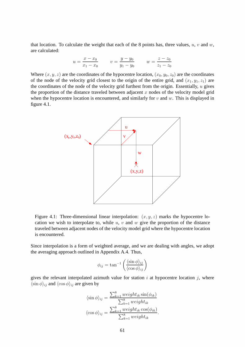
that location. To calculate the weight that each of the 8 points has, three values,u, v andw,are calculated:
u =x− x0
x1 − x0
v =y − y0
y1 − y0
w =z − z0z1 − z0
Where(x, y, z) are the coordinates of the hypocentre location,(x0, y0, z0) are the coordinatesof the node of the velocity grid closest to the origin of the entire grid, and(x1, y1, z1) arethe coordinates of the node of the velocity grid furthest from the origin. Essentially,u givesthe proportion of the distance traveled between adjacentx nodes of the velocity model gridwhen the hypocentre location is encountered, and similarlyfor v andw. This is displayed infigure 4.1.
0
u
w
v
(x,y,z)
0 0(x ,y ,z )
Figure 4.1: Three-dimensional linear interpolation:(x, y, z) marks the hypocentre lo-cation we wish to interpolate to, whileu, v andw give the proportion of the distancetraveled between adjacent nodes of the velocity model grid where the hypocentre locationis encountered.
Since interpolation is a form of weighted average, and we aredealing with angles, we adoptthe averaging approach outlined in Appendix A.4. Thus,
φij = tan−1
( 〈sinφ〉ij〈cosφ〉ij
)
gives the relevant interpolated azimuth value for stationi at hypocentre locationj, where〈sinφ〉ij and〈cosφ〉ij are given by
〈sinφ〉ij =
∑8k=1weightik sin(φik)∑8
k=1weightik
〈cosφ〉ij =
∑8k=1weightik cos(φik)∑8
k=1weightik.
61
whereφik is the azimuth for stationi at thekth of the surrounding 8 nodes of the velocitymodel grid surrounding locationxj, andweight is given by:
+ (1 − u)v · w · quali5 + u(1 − v)w · quali6+ u · v(1 − w)quali7 + u · v · w · quali8 (4.1)
Further,
θij = cos−1
〈cos θ〉ij√
〈sin θ cosφ〉2ij + 〈sin θ sinφ〉2ij + 〈cos θ〉2ij
gives the interpolated take-off angle for stationi at hypocentre locationj, where
〈cos θ〉ij =
∑8k=1weightik cos(θik)∑8
k=1weightik
〈sin θ cosφ〉ij =
∑8k=1weightik sin(θik) cos(φik)
∑8k=1weightik
〈sin θ sinφ〉ij =
∑8k=1weightik sin(θik) sin(φik)
∑8k=1weightik
whereφik andθik are the azimuth and take-off angle respectively for stationi at thekth of thesurrounding 8 nodes of the velocity model grid, andweight is given in Equation 4.1.
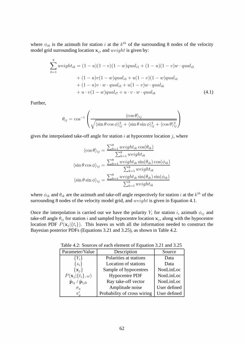
Once the interpolation is carried out we have the polarityYi for stationi, azimuthφij andtake-off angleθij for stationi and sampled hypocentre locationxj , along with the hypocentrelocation PDFP (xj|{ti}). This leaves us with all the information needed to constructtheBayesian posterior PDFs (Equations 3.21 and 3.25), as shownin Table 4.2.
Table 4.2: Sources of each element of Equation 3.21 and 3.25Parameter/Value Description Source
{Yi} Polarities at stations Data{si} Location of stations Data{xj} Sample of hypocentres NonLinLoc
P (xj |{ti}, ω) Hypocentre PDF NonLinLocpij / pijk Ray take-off vector NonLinLoc
σa Amplitude noise User definedπ′
p Probability of cross wiring User defined
62
4.3 Velest
Velest is a program that uses acoupled hypocentre-velocity modelmethod to determinemini-mum 1-dimensional velocity models. Velest is used in this project to obtain a random sampleof velocity models from a given priorP (υ), as is required in Equation 3.25.
The coupled hypocentre-velocity model method is similar toTarantola & Valette (1982)’sBayesian method of hypocentre location described in Section 3.2.2 and implemented in Non-LinLoc. The difference is that here it is assumed the velocity model is unknown to beginwith, and a solution for the velocity model is solved simultaneously with hypocentre loca-tions (Kissling 1988).
An indication of the quality of a velocity model can be given by the differencetresi between
the observed and theoretical arrival times at stationi
tresi = tobs
i − tcali (4.2)
where the theoretical arrival timestcali = tcal
i (x, T, υ, yi), depend on an estimated hypocentrelocationx, estimated origin timeT, the implemented velocity modelυ and station locationsyi. The observed arrival timestobs
i = tobsi (x0,T0, υ0, yi) depend on the true hypocentre loca-
tionx0, true origin timeT0, the true velocity modelυ0 and station locationsyi (Kissling 1988).
Velest takes an initial input velocity model and hypocentrelocations and uses this to calculatearrival timestcal
i . The program then adjusts hypocentral and velocity model parameters. Todo this, a relationship betweentres
i and the required adjustments is established. A first orderTaylor series expansion oftobs
i about the estimated parameters(x0 = x,T0 = T, υ0 = υ, yi =yi) gives
tobsi (x0,T0, υ0, yi) = tobs
i (x, T, υ, yi) +∂ti∂x
(x0 − x) +∂ti∂T
(T0 − T) +∂ti∂υ
(υ0 − υ)
+∂ti∂yi
(yi − yi)
= tobsi (x, T, υ, yi) +
∂ti∂x
(x0 − x) +∂ti∂T
(T0 − T) +∂ti∂υ
(υ0 − υ)
Substituting this into Equation 4.2 gives
tresi = tobs
i (x, T, υ, yi) +∂ti∂x
(x0 − x) +∂ti∂T
(T0 − T) +∂ti∂υ
(υ0 − υ) − tcali (x, T, υ, yi)
=∂ti∂x
(x0 − x) +∂ti∂T
(T0 − T) +∂ti∂υ
(υ0 − υ) (sincetobsi (x, T, υ, yi) = tcal
i (x, T, υ, yi))
=∂ti∂x
∆x +∂ti∂T
∆T +∂ti∂υ
∆υ (4.3)
where∆x is the required adjustment in estimated hypocentre location,∆T is the adjustment inestimated origin time, and∆υ is the adjustment in the velocity model (Kissling 1988, Kissling,Ellsworth, Eberhart-Phillips & Kradolfer 1994).
63
The minimum 1D velocity model is the velocity model with minimum root mean square(RMS) misfit of{tres
i }, where RMS is defined as
RMS(tresi ) =
√
1
n
∑
i
(tresi )2
This minimum 1D velocity model is given by solving Equation 4.3. This equation is non-linear, and hence is solved numerically by Velest (Kissling1988).
The iterative procedure of Velest is as follows:
1. Solve the coupled hypocentre-velocity model problem forthe estimated hypocentresand velocity model. This gives adjusted hypocentres and an adjusted velocity model;
2. Recalculatetcali based on these adjustments;
3. Check the RMS of the new velocity model — if it is lower, retain it. Return to 1.
Due to the non-linearity of the coupled hypocentre-velocity method, multiple local RMS min-ima may occur over the velocity model solution space. Different input models may find differ-ent local minima. A priori it is unknown where these minima occur so a number of Velest runsare conducted using a variety of different input velocity models, resulting in a set of minimum1D velocity models (Kissling 1995, Clarke 2007). Further specific details on how Velest wasrun in this project are given in Section 5.2.2.
4.4 Grid Computing
As mentioned in Section 3.3.2, the VMU posterior PDF (Equation 3.25) is calculated usingMonte Carlo integration; summing overp different VMK posterior PDFs. Calculation of thisis particularly computationally intensive given the largesample of velocity models used in thisproject (p ≃ 1000). Running the required programs and models on one machine would takeseveral days. To reduce this computation time we make use of the School of Mathematics,Statistics and Computer Science’s computational grid, which comprises approximately 170NetBSD (Unix) workstations.
The grid is particularly useful for multiple runs of the sameprogram with differing parametervalues, as is the case here. We break the job down into sets of 10 velocity models, and haveeach computer on the grid evaluate the VMK posterior PDF for its set of 10 models. We thenretrieve each VMK posterior PDF from the grid and sum over all∼ 1000 to obtain the VMUposterior PDF. This reduces the computation time from days to hours.
64
Chapter 5
Applications
In this chapter we discuss the application of our Bayesian methods of focal mechanism estima-tion to earthquake phase data from New Zealand. We consider two cases; the velocity modelknown case, with data from the Raukumara Peninsula, and the velocity model unknown case,with data from Kawerau.
5.1 Velocity model known — Raukumara Peninsula
We will use data from the Raukumara Peninsula, New Zealand, to illustrate the case in whichwe presume that the uncertainties in the hypocentre location are caused solely by P-wavearrival timing errors, and that the velocity model is error-free and known. The RaukumaraPeninsula is particularly suitable to study this objective, as the 3-dimensionalVp (P-wavevelocity) andVs (S-wave velocity) structures of the area have been determined by Reynerset al. (1999).
5.1.1 Tectonic Setting
New Zealand lies at the boundary of the Pacific and Australiantectonic plates. To the east ofthe North Island, the Pacific plate subducts beneath the overlying Australian plate. The twoplates converge at approximately 45 mm/yr in the region of interest; the Raukumara Peninsula,on the East Cape of the North Island of New Zealand. The plate interface occurs at a depth ofapproximately 15 km beneath the east of the Raukumara Peninsula (Reyners et al. 1999).
The Raukumara Peninsula (see Figure 5.1) lies 300 km southwest of the Tonga-Kermadecand Hikurangi subduction zone junction. At this junction, crust to the north experiences sub-duction along the Kermadec Trench, while to the south the subduction is influenced by theHikurangi Plateau (Reyners & McGinty 1999).
5.1.2 Velocity Model
The velocity model we use here is based on a 3D velocity model obtained by Reyners et al.(1999). In a previous study by Reyners & McGinty (1999), 36 seismographs were deployedover the Raukumara Peninsula between July and December 1994, the data from which en-
65
176˚
176˚
177˚
177˚
178˚
178˚
179˚
179˚
-40˚ -40˚
-39˚ -39˚
-38˚ -38˚
-37˚ -37˚
176˚
176˚
177˚
177˚
178˚
178˚
179˚
179˚
-40˚ -40˚
-39˚ -39˚
-38˚ -38˚
-37˚ -37˚
0 50
km
Figure 5.1: Map of the Raukumara Peninsula. Symbols show theboundary of the Reynerset al. (1999) velocity model (dark red line), temporary seismometers deployed by Reyners& McGinty (1999) (white triangles), and permanent seismometers within the velocitymodel bounds as at time of the Reyners & McGinty (1999) study (red squares).
66
abled Reyners et al. (1999) to determine theVp andVs structure of the region.
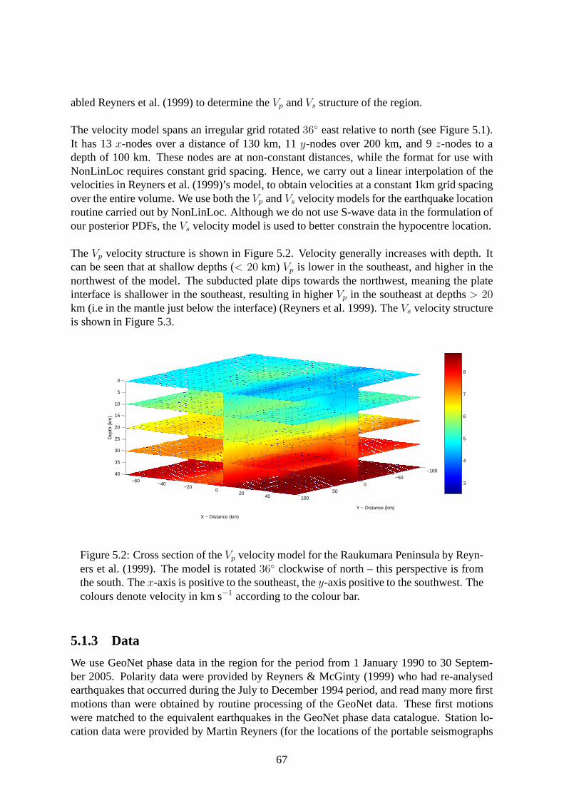
The velocity model spans an irregular grid rotated36◦ east relative to north (see Figure 5.1).It has 13x-nodes over a distance of 130 km, 11y-nodes over 200 km, and 9z-nodes to adepth of 100 km. These nodes are at non-constant distances, while the format for use withNonLinLoc requires constant grid spacing. Hence, we carry out a linear interpolation of thevelocities in Reyners et al. (1999)’s model, to obtain velocities at a constant 1km grid spacingover the entire volume. We use both theVp andVs velocity models for the earthquake locationroutine carried out by NonLinLoc. Although we do not use S-wave data in the formulation ofour posterior PDFs, theVs velocity model is used to better constrain the hypocentre location.
TheVp velocity structure is shown in Figure 5.2. Velocity generally increases with depth. Itcan be seen that at shallow depths (< 20 km) Vp is lower in the southeast, and higher in thenorthwest of the model. The subducted plate dips towards thenorthwest, meaning the plateinterface is shallower in the southeast, resulting in higher Vp in the southeast at depths> 20km (i.e in the mantle just below the interface) (Reyners et al. 1999). TheVs velocity structureis shown in Figure 5.3.
−60−40
−200
2040
−100−50
050
100
0
5
10
15
20
25
30
35
40
Y − Distance (km)
X − Distance (km)
Dep
th (
km)
3
4
5
6
7
8
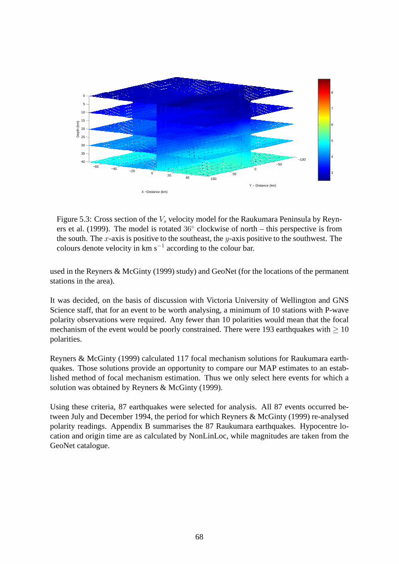
Figure 5.2: Cross section of theVp velocity model for the Raukumara Peninsula by Reyn-ers et al. (1999). The model is rotated36◦ clockwise of north – this perspective is fromthe south. Thex-axis is positive to the southeast, they-axis positive to the southwest. Thecolours denote velocity in km s−1 according to the colour bar.
5.1.3 Data
We use GeoNet phase data in the region for the period from 1 January 1990 to 30 Septem-ber 2005. Polarity data were provided by Reyners & McGinty (1999) who had re-analysedearthquakes that occurred during the July to December 1994 period, and read many more firstmotions than were obtained by routine processing of the GeoNet data. These first motionswere matched to the equivalent earthquakes in the GeoNet phase data catalogue. Station lo-cation data were provided by Martin Reyners (for the locations of the portable seismographs
67
−60−40
−200
2040
−100−50
050
100
0
5
10
15
20
25
30
35
40
Y − Distance (km)
X −Distance (km)
Dep
th (
km)
3
4
5
6
7
8
Figure 5.3: Cross section of theVs velocity model for the Raukumara Peninsula by Reyn-ers et al. (1999). The model is rotated36◦ clockwise of north – this perspective is fromthe south. Thex-axis is positive to the southeast, they-axis positive to the southwest. Thecolours denote velocity in km s−1 according to the colour bar.
used in the Reyners & McGinty (1999) study) and GeoNet (for the locations of the permanentstations in the area).
It was decided, on the basis of discussion with Victoria University of Wellington and GNSScience staff, that for an event to be worth analysing, a minimum of 10 stations with P-wavepolarity observations were required. Any fewer than 10 polarities would mean that the focalmechanism of the event would be poorly constrained. There were 193 earthquakes with≥ 10polarities.
Reyners & McGinty (1999) calculated 117 focal mechanism solutions for Raukumara earth-quakes. Those solutions provide an opportunity to compare our MAP estimates to an estab-lished method of focal mechanism estimation. Thus we only select here events for which asolution was obtained by Reyners & McGinty (1999).
Using these criteria, 87 earthquakes were selected for analysis. All 87 events occurred be-tween July and December 1994, the period for which Reyners & McGinty (1999) re-analysedpolarity readings. Appendix B summarises the 87 Raukumara earthquakes. Hypocentre lo-cation and origin time are as calculated by NonLinLoc, whilemagnitudes are taken from theGeoNet catalogue.
68
87Events with>= 10 polarities
193117
Events with a solutionin Reyners &McGinty (1999)
Our selected events
Figure 5.4: Diagram showing our event selection criteria. For an event to be selected, itmust have≥ 10 polarity readings, and must have a corresponding solution by Reyners &McGinty (1999).
5.1.4 Posterior PDF Particulars
Recall that the posterior probability for the velocity model known case is given by Equa-tion 3.21:
P (Θ|d, ω) ∝ P (Θ)
∫∫ m∑
j=1
[
n∏
i=1
π1
2(1+si)
ij (1 − πij)1
2(1−si)
]
P (σa)P (πp)dσa dπp
We calculate this posterior PDF for all 87 events, under the following conditions:
• a uniform prior onΘ: P (Θ) ∝ sin θ ⇔ P (R(Θ)) ∝ 1
• P (σa) = δ(σa−σa0), andP (πp) = δ(πp−πp0
) whereδ denotes the Dirac delta functionandσa0
andπp0are values forσa andπp, assumed to be known. Due to the properties
of the delta function (see Appendix A.9), the posterior PDF becomes
P (Θ|d, ω) ∝ P (Θ)m∑
j=1
[
n∏
i=1
π1
2(1+yi)
ij (1 − πij)1
2(1−yi)
]
whereπij is given by
πij = π′p0
+ (1 − 2π′p0
)Φ
(
2(pij · n)(pij · u)
σa0
)
This approach is equivalent to taking fixed values forσa andπp. For this to be valid werequire appropriate values for these parameters.
While the rate of polarity errors varies between datasets, we take the value used by Hardebeck& Shearer (2002), who found that around 20% of ambiguously determined polarities wereinconsistent. Thus we take a (conservative) value ofπ′
p0= 0.2.
For the amplitude noiseσa we take a value ofσa0= 1
6, based on values in Zollo & Bernard
(1991) and Brillinger et al. (1980).
69
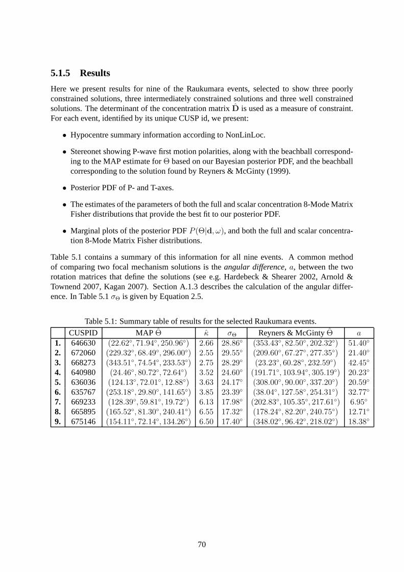
5.1.5 Results
Here we present results for nine of the Raukumara events, selected to show three poorlyconstrained solutions, three intermediately constrainedsolutions and three well constrainedsolutions. The determinant of the concentration matrixD is used as a measure of constraint.For each event, identified by its unique CUSP id, we present:
• Hypocentre summary information according to NonLinLoc.
• Stereonet showing P-wave first motion polarities, along with the beachball correspond-ing to the MAP estimate forΘ based on our Bayesian posterior PDF, and the beachballcorresponding to the solution found by Reyners & McGinty (1999).
• Posterior PDF of P- and T-axes.
• The estimates of the parameters of both the full and scalar concentration 8-Mode MatrixFisher distributions that provide the best fit to our posterior PDF.
• Marginal plots of the posterior PDFP (Θ|d, ω), and both the full and scalar concentra-tion 8-Mode Matrix Fisher distributions.
Table 5.1 contains a summary of this information for all nineevents. A common methodof comparing two focal mechanism solutions is theangular difference, a, between the tworotation matrices that define the solutions (see e.g. Hardebeck & Shearer 2002, Arnold &Townend 2007, Kagan 2007). Section A.1.3 describes the calculation of the angular differ-ence. In Table 5.1σΘ is given by Equation 2.5.
Table 5.1: Summary table of results for the selected Raukumara events.
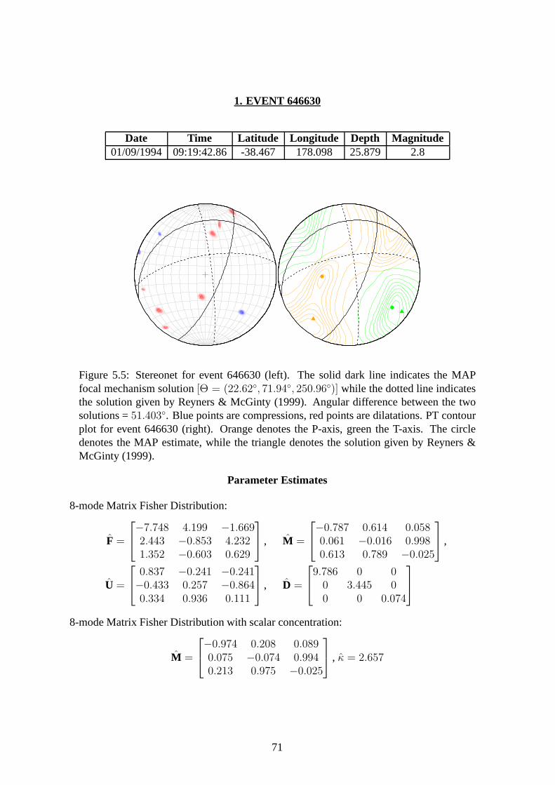
Date Time Latitude Longitude Depth Magnitude01/09/1994 09:19:42.86 -38.467 178.098 25.879 2.8
Figure 5.5: Stereonet for event 646630 (left). The solid dark line indicates the MAPfocal mechanism solution[Θ = (22.62◦, 71.94◦, 250.96◦)] while the dotted line indicatesthe solution given by Reyners & McGinty (1999). Angular difference between the twosolutions =51.403◦. Blue points are compressions, red points are dilatations.PT contourplot for event 646630 (right). Orange denotes the P-axis, green the T-axis. The circledenotes the MAP estimate, while the triangle denotes the solution given by Reyners &McGinty (1999).
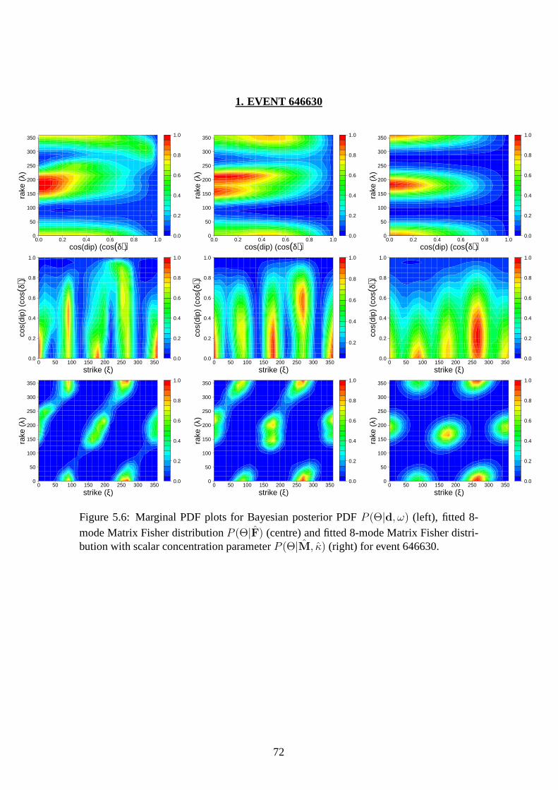
Figure 5.6: Marginal PDF plots for Bayesian posterior PDFP (Θ|d, ω) (left), fitted 8-
mode Matrix Fisher distributionP (Θ|F) (centre) and fitted 8-mode Matrix Fisher distri-bution with scalar concentration parameterP (Θ|M, κ) (right) for event 646630.
72
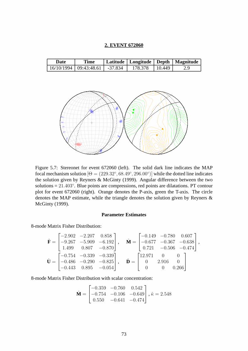
2. EVENT 672060
Date Time Latitude Longitude Depth Magnitude16/10/1994 09:43:48.61 -37.834 178.378 10.449 2.9
Figure 5.7: Stereonet for event 672060 (left). The solid dark line indicates the MAPfocal mechanism solution[Θ = (229.32◦, 68.49◦, 296.00◦)] while the dotted line indicatesthe solution given by Reyners & McGinty (1999). Angular difference between the twosolutions =21.403◦. Blue points are compressions, red points are dilatations.PT contourplot for event 672060 (right). Orange denotes the P-axis, green the T-axis. The circledenotes the MAP estimate, while the triangle denotes the solution given by Reyners &McGinty (1999).
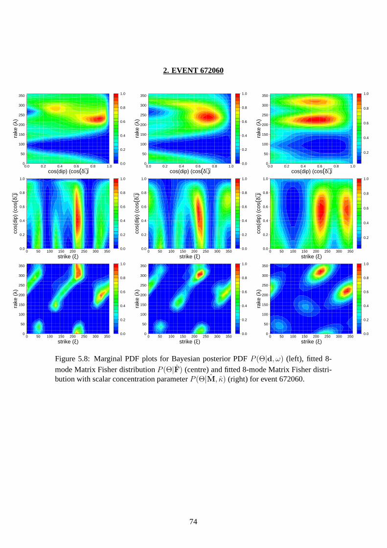
Figure 5.8: Marginal PDF plots for Bayesian posterior PDFP (Θ|d, ω) (left), fitted 8-
mode Matrix Fisher distributionP (Θ|F) (centre) and fitted 8-mode Matrix Fisher distri-bution with scalar concentration parameterP (Θ|M, κ) (right) for event 672060.
74
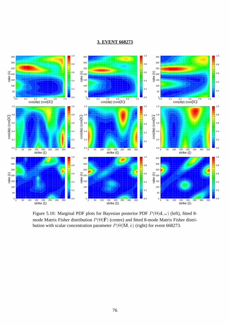
3. EVENT 668273
Date Time Latitude Longitude Depth Magnitude02/10/1994 22:38:48.96 -37.866 178.084 30.957 2.9
Figure 5.9: Stereonet for event 668273 (left). The solid dark line indicates the MAPfocal mechanism solution[Θ = (343.51◦, 74.54◦, 233.53◦)] while the dotted line indicatesthe solution given by Reyners & McGinty (1999). Angular difference between the twosolutions =42.45◦. Blue points are compressions, red points are dilatations.PT contourplot for event 668273 (right). Orange denotes the P-axis, green the T-axis. The circledenotes the MAP estimate, while the triangle denotes the solution given by Reyners &McGinty (1999).
Figure 5.10: Marginal PDF plots for Bayesian posterior PDFP (Θ|d, ω) (left), fitted 8-
mode Matrix Fisher distributionP (Θ|F) (centre) and fitted 8-mode Matrix Fisher distri-bution with scalar concentration parameterP (Θ|M, κ) (right) for event 668273.
76
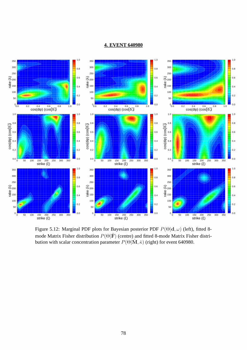
4. EVENT 640980
Date Time Latitude Longitude Depth Magnitude21/08/1994 13:36:52.95 -38.198 178.14 18.018 2.8
Figure 5.11: Stereonet for event 640980 (left). The solid dark line indicates the MAPfocal mechanism solution[Θ = (24.46◦, 80.72◦, 72.64◦)] while the dotted line indicatesthe solution given by Reyners & McGinty (1999). Angular difference between the twosolutions =20.229◦. Blue points are compressions, red points are dilatations.PT contourplot for event 640980 (right). Orange denotes the P-axis, green the T-axis. The circledenotes the MAP estimate, while the triangle denotes the solution given by Reyners &McGinty (1999).
Figure 5.12: Marginal PDF plots for Bayesian posterior PDFP (Θ|d, ω) (left), fitted 8-
mode Matrix Fisher distributionP (Θ|F) (centre) and fitted 8-mode Matrix Fisher distri-bution with scalar concentration parameterP (Θ|M, κ) (right) for event 640980.
78
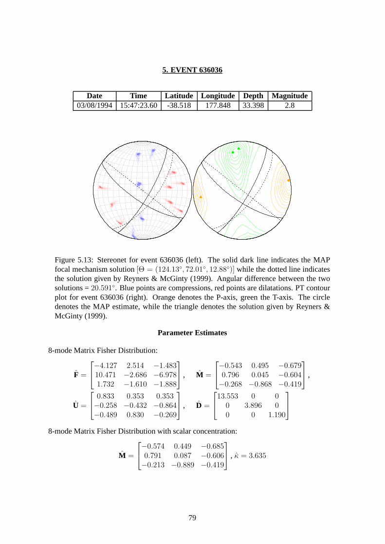
5. EVENT 636036
Date Time Latitude Longitude Depth Magnitude03/08/1994 15:47:23.60 -38.518 177.848 33.398 2.8
Figure 5.13: Stereonet for event 636036 (left). The solid dark line indicates the MAPfocal mechanism solution[Θ = (124.13◦, 72.01◦, 12.88◦)] while the dotted line indicatesthe solution given by Reyners & McGinty (1999). Angular difference between the twosolutions =20.591◦. Blue points are compressions, red points are dilatations.PT contourplot for event 636036 (right). Orange denotes the P-axis, green the T-axis. The circledenotes the MAP estimate, while the triangle denotes the solution given by Reyners &McGinty (1999).
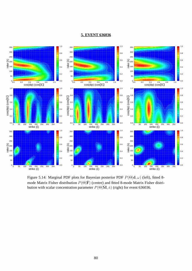
Figure 5.14: Marginal PDF plots for Bayesian posterior PDFP (Θ|d, ω) (left), fitted 8-
mode Matrix Fisher distributionP (Θ|F) (centre) and fitted 8-mode Matrix Fisher distri-bution with scalar concentration parameterP (Θ|M, κ) (right) for event 636036.
80
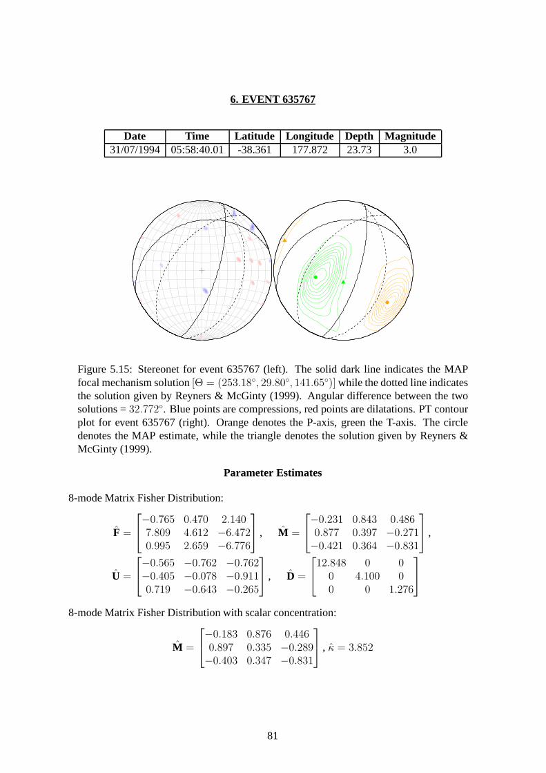
6. EVENT 635767
Date Time Latitude Longitude Depth Magnitude31/07/1994 05:58:40.01 -38.361 177.872 23.73 3.0
Figure 5.15: Stereonet for event 635767 (left). The solid dark line indicates the MAPfocal mechanism solution[Θ = (253.18◦, 29.80◦, 141.65◦)] while the dotted line indicatesthe solution given by Reyners & McGinty (1999). Angular difference between the twosolutions =32.772◦. Blue points are compressions, red points are dilatations.PT contourplot for event 635767 (right). Orange denotes the P-axis, green the T-axis. The circledenotes the MAP estimate, while the triangle denotes the solution given by Reyners &McGinty (1999).
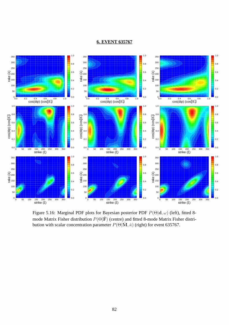
Figure 5.16: Marginal PDF plots for Bayesian posterior PDFP (Θ|d, ω) (left), fitted 8-
mode Matrix Fisher distributionP (Θ|F) (centre) and fitted 8-mode Matrix Fisher distri-bution with scalar concentration parameterP (Θ|M, κ) (right) for event 635767.
82
7. EVENT 669233
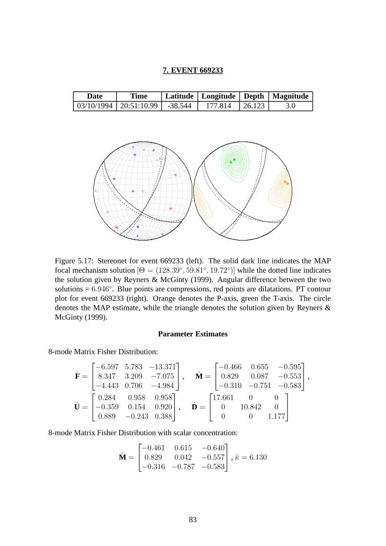
Date Time Latitude Longitude Depth Magnitude03/10/1994 20:51:10.99 -38.544 177.814 26.123 3.0
Figure 5.17: Stereonet for event 669233 (left). The solid dark line indicates the MAPfocal mechanism solution[Θ = (128.39◦, 59.81◦, 19.72◦)] while the dotted line indicatesthe solution given by Reyners & McGinty (1999). Angular difference between the twosolutions =6.946◦. Blue points are compressions, red points are dilatations.PT contourplot for event 669233 (right). Orange denotes the P-axis, green the T-axis. The circledenotes the MAP estimate, while the triangle denotes the solution given by Reyners &McGinty (1999).
Figure 5.18: Marginal PDF plots for Bayesian posterior PDFP (Θ|d, ω) (left), fitted 8-
mode Matrix Fisher distributionP (Θ|F) (centre) and fitted 8-mode Matrix Fisher distri-bution with scalar concentration parameterP (Θ|M, κ) (right) for event 669233.
84
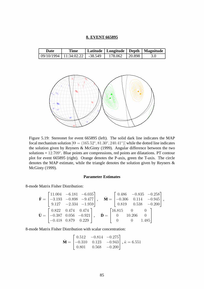
8. EVENT 665895
Date Time Latitude Longitude Depth Magnitude09/10/1994 11:34:02.22 -38.549 178.062 20.898 3.0
Figure 5.19: Stereonet for event 665895 (left). The solid dark line indicates the MAPfocal mechanism solution[Θ = (165.52◦, 81.30◦, 240.41◦)] while the dotted line indicatesthe solution given by Reyners & McGinty (1999). Angular difference between the twosolutions =12.709◦. Blue points are compressions, red points are dilatations.PT contourplot for event 665895 (right). Orange denotes the P-axis, green the T-axis. The circledenotes the MAP estimate, while the triangle denotes the solution given by Reyners &McGinty (1999).
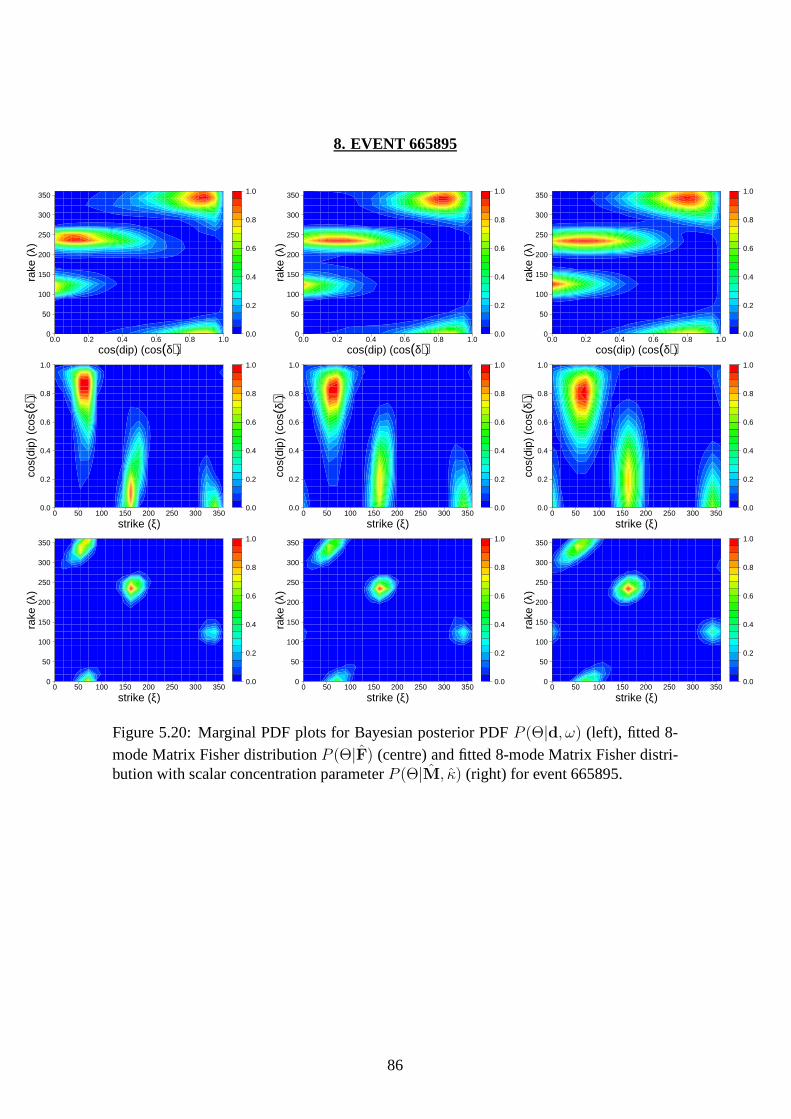
Figure 5.20: Marginal PDF plots for Bayesian posterior PDFP (Θ|d, ω) (left), fitted 8-
mode Matrix Fisher distributionP (Θ|F) (centre) and fitted 8-mode Matrix Fisher distri-bution with scalar concentration parameterP (Θ|M, κ) (right) for event 665895.
86
9. EVENT 675146
Date Time Latitude Longitude Depth Magnitude24/10/1994 01:18:43.58 -38.539 178.098 25.488 2.9
Figure 5.21: Stereonet for event 675146 (left). The solid dark line indicates the MAPfocal mechanism solution[Θ = (154.11◦, 72.14◦, 134.26◦)] while the dotted line indicatesthe solution given by Reyners & McGinty (1999). Angular difference between the twosolutions =18.377◦. Blue points are compressions, red points are dilatations.PT contourplot for event 675146 (right). Orange denotes the P-axis, green the T-axis. The circledenotes the MAP estimate, while the triangle denotes the solution given by Reyners &McGinty (1999).
Figure 5.22: Marginal PDF plots for Bayesian posterior PDFP (Θ|d, ω) (left), fitted 8-
mode Matrix Fisher distributionP (Θ|F) (centre) and fitted 8-mode Matrix Fisher distri-bution with scalar concentration parameterP (Θ|M, κ) (right) for event 675146.
88
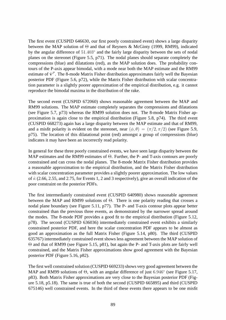
The first event (CUSPID 646630, our first poorly constrained event) shows a large disparitybetween the MAP solution ofΘ and that of Reyners & McGinty (1999, RM99), indicatedby the angular difference of51.403◦ and the fairly large disparity between the sets of nodalplanes on the stereonet (Figure 5.5, p71). The nodal planes should separate completely thecompressions (blue) and dilatations (red), as the MAP solution does. The probability con-tours of the P-axis appear bimodal, with a mode near both the MAP estimate and the RM99estimate ofvP . The 8-mode Matrix Fisher distribution approximates fairly well the Bayesianposterior PDF (Figure 5.6, p72), while the Matrix Fisher distribution with scalar concentra-tion parameter is a slightly poorer approximation of the empirical distribution, e.g. it cannotreproduce the bimodal maxima in the distribution of the rake.
The second event (CUSPID 672060) shows reasonable agreement between the MAP andRM99 solutions. The MAP estimate completely separates the compressions and dilatations(see Figure 5.7, p73) whereas the RM99 solution does not. The8-mode Matrix Fisher ap-proximation is again close to the empirical distribution (Figure 5.8, p74). The third event(CUSPID 668273) again has a large disparity between the MAP estimate and that of RM99,and a misfit polarity is evident on the stereonet, near(φ, θ) = (π/2, π/2) (see Figure 5.9,p75). The location of this dilatational point (red) amongsta group of compressions (blue)indicates it may have been an incorrectly read polarity.
In general for these three poorly constrained events, we have seen large disparity between theMAP estimates and the RM99 estimates ofΘ. Further, the P- and T-axis contours are poorlyconstrained and can cross the nodal planes. The 8-mode Matrix Fisher distribution providesa reasonable approximation to the empirical distribution,and the Matrix Fisher distributionwith scalar concentration parameter provides a slightly poorer approximation. The low valuesof κ (2.66, 2.55, and 2.75, for Events 1, 2 and 3 respectively), give an overall indication of thepoor constraint on the posterior PDFs.
The first intermediately constrained event (CUSPID 640980)shows reasonable agreementbetween the MAP and RM99 solutions ofΘ. There is one polarity reading that crosses anodal plane boundary (see Figure 5.11, p77). The P- and T-axis contour plots appear betterconstrained than the previous three events, as demonstrated by the narrower spread aroundthe modes. The 8-mode PDF provides a good fit to the empirical distribution (Figure 5.12,p78). The second (CUSPID 636036) intermediately constrained event exhibits a similarlyconstrained posterior PDF, and here the scalar concentration PDF appears to be almost asgood an approximation as the full Matrix Fisher (Figure 5.14, p80). The third (CUSPID635767) intermediately constrained event shows less agreement between the MAP solution ofΘ and that of RM99 (see Figure 5.15, p81), but again the P- and T-axis plots are fairly wellconstrained, and the Matrix Fisher approximations show good agreement with the Bayesianposterior PDF (Figure 5.16, p82).
The first well constrained solution (CUSPID 669233) shows very good agreement between theMAP and RM99 solutions ofΘ, with an angular difference of just6.946◦ (see Figure 5.17,p83). Both Matrix Fisher approximations are very close to the Bayesian posterior PDF (Fig-ure 5.18, p5.18). The same is true of both the second (CUSPID 665895) and third (CUSPID675146) well constrained events. In the third of these events there appears to be one misfit
89
polarity (see the upper left quadrant of Figure 5.21, p87). The well constrained events arecharacterised by highκ (6.13, 6.55 and 6.50) compared to the poorer constrained events. TheP- and T-axis contours of all three events are tightly constrained. In general the well con-strained events have a higher number of polarity readings and better focal sphere coveragethan the poorly and intermediately constrained events.
The better constrained events agree closely the established focal mechanism solutions ofRM99. The Matrix Fisher approximation tends to match well the Bayesian posterior PDF,with the match appearing better for well constrained events. The full 8-mode Matrix Fisherdistribution with parameter matrixF generally provides a better fit than the scalar concentra-tion version, at the cost of longer computation time and increased complexity, although thedifference in quality of fit is small for the better constrained events.
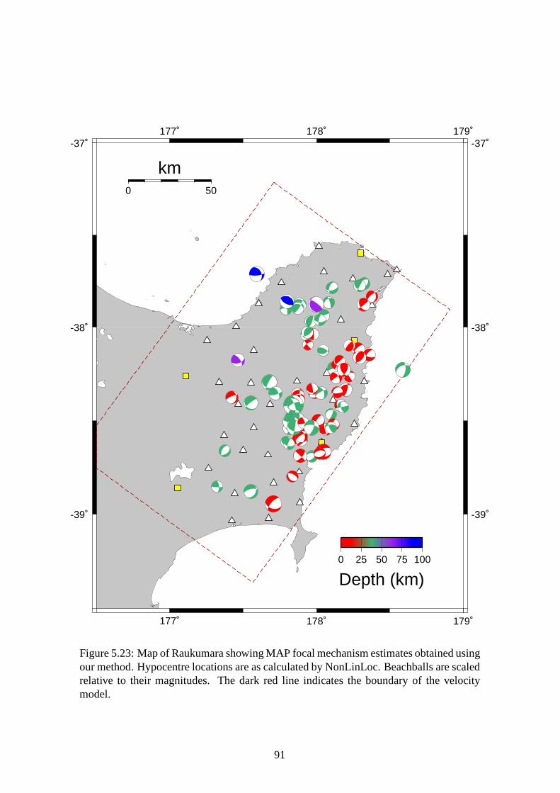
Figure 5.23 shows a map of all 87 MAP focal mechanism estimates obtained in this study.The map corresponds closely to Figure 5.24, the solutions obtained in the RM99 study, exceptfor some small discrepancies which we discuss below.
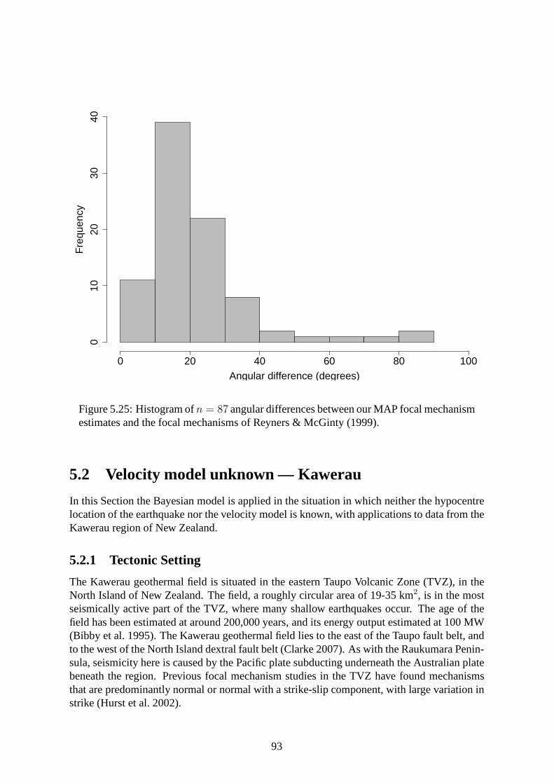
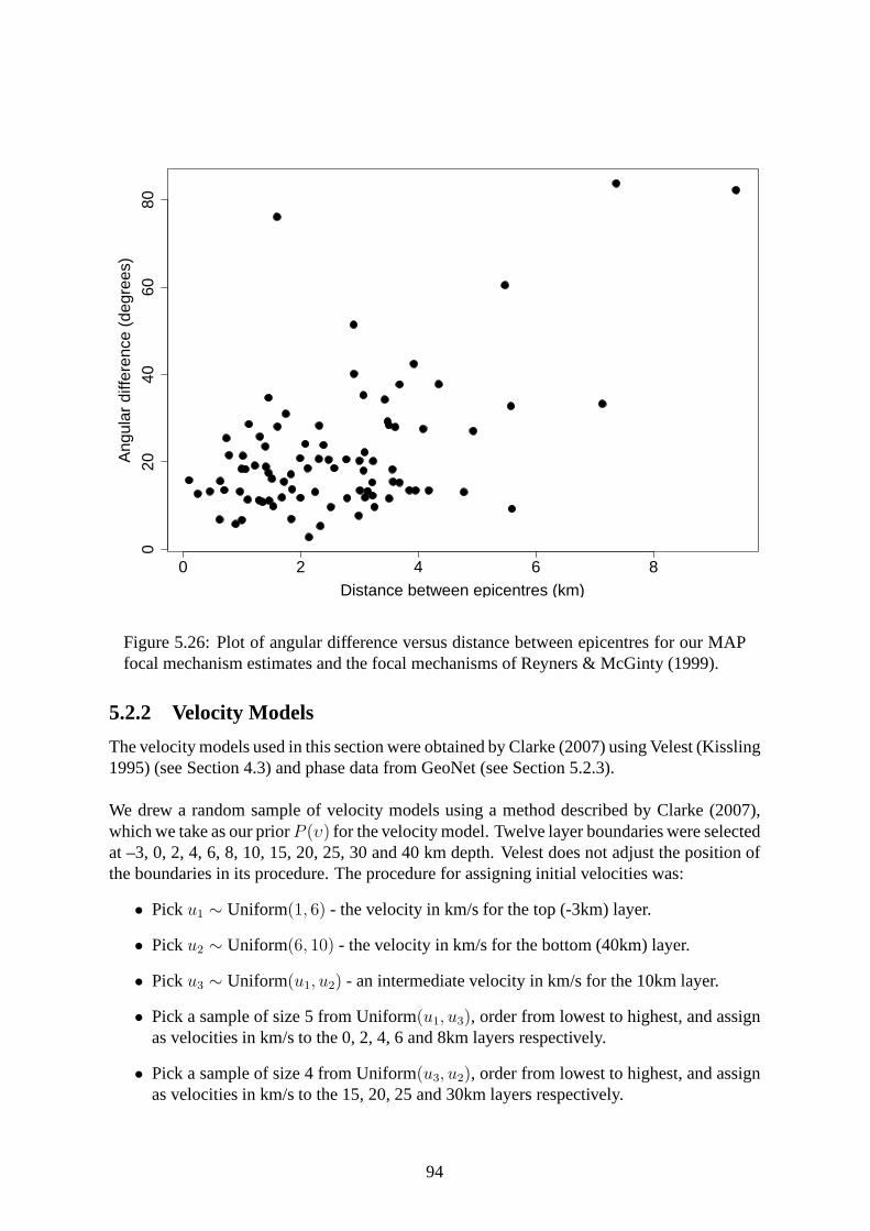
Figure 5.25 shows a histogram of angular differences between our solutions and those ofRM99. For 75% of events, the solutions are within27.3◦ of each other, indicating that solu-tions obtained by our method are generally similar to those obtained by RM99. The angulardifferences between the two sets may be partly explained by the different focal mechanismestimation methodology used and the hypocentral uncertainties considered here, but may alsobe partly explained by differences in hypocentre location resulting from our interpolation ofthe Reyners et al. (1999) velocity model to a constant grid spacing. Figure 5.26 shows a plotof angular difference between solutions versus the distance between the epicentres as locatedby RM99 and NonLinLoc in this study. There is no obvious relationship evident.
90
177˚
177˚
178˚
178˚
179˚
179˚
-39˚ -39˚
-38˚ -38˚
-37˚ -37˚
0 50
km
0 25 50 75 100
Depth (km)
Figure 5.23: Map of Raukumara showing MAP focal mechanism estimates obtained usingour method. Hypocentre locations are as calculated by NonLinLoc. Beachballs are scaledrelative to their magnitudes. The dark red line indicates the boundary of the velocitymodel.
91
177˚
177˚
178˚
178˚
179˚
179˚
-39˚ -39˚
-38˚ -38˚
-37˚ -37˚
0 50
km
0 25 50 75 100
Depth (km)
Figure 5.24: Map of Raukumara showing focal mechanisms obtained by Reyners &McGinty (1999). Hypocentre locations also from Reyners & McGinty (1999). Beach-balls are scaled relative to their magnitudes. The dark red line indicates the boundary ofthe velocity model.
92
Angular difference (degrees)
Fre
quen
cy
0 20 40 60 80 100
010
2030
40
Figure 5.25: Histogram ofn = 87 angular differences between our MAP focal mechanismestimates and the focal mechanisms of Reyners & McGinty (1999).
5.2 Velocity model unknown — Kawerau
In this Section the Bayesian model is applied in the situation in which neither the hypocentrelocation of the earthquake nor the velocity model is known, with applications to data from theKawerau region of New Zealand.
5.2.1 Tectonic Setting
The Kawerau geothermal field is situated in the eastern TaupoVolcanic Zone (TVZ), in theNorth Island of New Zealand. The field, a roughly circular area of 19-35 km2, is in the mostseismically active part of the TVZ, where many shallow earthquakes occur. The age of thefield has been estimated at around 200,000 years, and its energy output estimated at 100 MW(Bibby et al. 1995). The Kawerau geothermal field lies to the east of the Taupo fault belt, andto the west of the North Island dextral fault belt (Clarke 2007). As with the Raukumara Penin-sula, seismicity here is caused by the Pacific plate subducting underneath the Australian platebeneath the region. Previous focal mechanism studies in theTVZ have found mechanismsthat are predominantly normal or normal with a strike-slip component, with large variation instrike (Hurst et al. 2002).
93
0 2 4 6 8
020
4060
80
Distance between epicentres (km)
Ang
ular
diff
eren
ce (
degr
ees)
Figure 5.26: Plot of angular difference versus distance between epicentres for our MAPfocal mechanism estimates and the focal mechanisms of Reyners & McGinty (1999).
5.2.2 Velocity Models
The velocity models used in this section were obtained by Clarke (2007) using Velest (Kissling1995) (see Section 4.3) and phase data from GeoNet (see Section 5.2.3).
We drew a random sample of velocity models using a method described by Clarke (2007),which we take as our priorP (υ) for the velocity model. Twelve layer boundaries were selectedat –3, 0, 2, 4, 6, 8, 10, 15, 20, 25, 30 and 40 km depth. Velest does not adjust the position ofthe boundaries in its procedure. The procedure for assigning initial velocities was:
• Picku1 ∼ Uniform(1, 6) - the velocity in km/s for the top (-3km) layer.
• Picku2 ∼ Uniform(6, 10) - the velocity in km/s for the bottom (40km) layer.
• Picku3 ∼ Uniform(u1, u2) - an intermediate velocity in km/s for the 10km layer.
• Pick a sample of size 5 from Uniform(u1, u3), order from lowest to highest, and assignas velocities in km/s to the 0, 2, 4, 6 and 8km layers respectively.
• Pick a sample of size 4 from Uniform(u3, u2), order from lowest to highest, and assignas velocities in km/s to the 15, 20, 25 and 30km layers respectively.
94
176˚
176˚
177˚
177˚
-39˚ -39˚
-38˚ -38˚
-37˚ -37˚
176˚
176˚
177˚
177˚
-39˚ -39˚
-38˚ -38˚
-37˚ -37˚
0 50
km
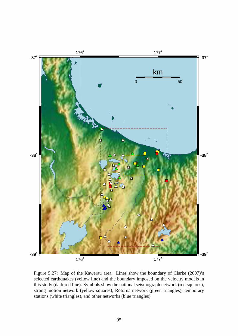
Figure 5.27: Map of the Kawerau area. Lines show the boundaryof Clarke (2007)’sselected earthquakes (yellow line) and the boundary imposed on the velocity models inthis study (dark red line). Symbols show the national seismograph network (red squares),strong motion network (yellow squares), Rotorua network (green triangles), temporarystations (white triangles), and other networks (blue triangles).
95
Selection of the intermediate velocity third means the models will have different gradients inthe upper and lower parts. This ensures a wide range of input models are selected (Clarke2007).
Clarke (2007) generated approximately 1000 P-wave velocity models in this manner, andused these as a basis for joint P- and S-wave velocity model inversions using Velest. Ini-tial P-wave velocities for this joint procedure were randomly selected within 1 standard de-viation of the mean in each layer from the P-wave only models.Initial S-wave velocitieswere chosen randomly, in a similar manner as the initial random P-wave models, except thatu1 ∼ Uniform(0, 3), u2 ∼ Uniform(3, 9), andVp ≥ Vs in every layer. For our hypocentrelocation routine we use the models output from the joint P- and S-wave inversion. These 1000models are shown in Figure 5.28.
0 2 4 6 8 10
4030
2010
0
Velocity (km/s)
Dep
th (
km)
Figure 5.28: Plot of 1000 P- (black) and S-wave (blue) velocity models for Kawerau, asobtained by (Clarke 2007) using Velest. The solid red line marks the mean velocity ineach layer, while the dashed lines mark one standard deviation from the mean.
Velest also outputs station corrections for each model, which are values oftresi for a given ve-
locity model and stationi, averaged over all events (Kissling 1995). These station correctionsadjust for the true 3D variation in velocity that a 1D model cannot account for.
We convert the 1D velocity models to 3D for use with NonLinLoc, using theVel2Grid pro-gram. This requires us to select the bounds for the model, as a1D velocity model inherently
96
has none. As stations must be inside the model bounds forGrid2Time to calculate theirtake-off angles, we use the tightest constraints on latitude and longitude such that all stationsfor which polarities are recorded are encompassed by the model. This gives us latitude boundsof −37.73◦ to−38.92◦, and longitude bounds of176.26◦ to 177.12◦, while we take a depth of50 km as a lower boundary.
5.2.3 Data
Since the velocity models we will use are based on the research of Clarke (2007), we usehere the same phase data that was used in that study to construct the velocity models. UsingGeoNet phase data, Clarke (2007) selected earthquakes in the Kawerau region, with hypocen-tre latitudes between−38◦ and−38.2◦, longitudes between175.55◦ and176.85◦, and depthsshallower than 20 km. From this set of 1875 earthquakes, the most reliable events were se-lected. The selection criteria were:
• The event must have a minimum of 8 P-wave phases and 3 S-wave phases to ensure itis able to be located reliably.
• Seismic stations receiving waves from the event must have a maximum azimuthal gapof less than180◦ to guard against epicentral bias.
• The nearest station to the event must be maximum of 10km away from the epicentre(as determined by the GeoNet hypocentre location) to ensuredepth is determined accu-rately.
Meanwhile, we apply a further criterion that an event must have seven or more polarity read-ings to ensure adequate coverage of the focal sphere. This number is slightly relaxed from thevalue of 10 used in Section 5.1, as the GeoNet data contains relatively few polarity readings.This selection criterion narrows our set of earthquakes to seven.
5.2.4 Posterior PDF Particulars
We assign equal prior weight to each of the∼ 1000 velocity models, and these togetherconstitute our prior for the velocity modelP (υ). Further work can and should be put intoestablishing a better motivated prior for the velocity model, however for the purposes of thisproject we have simply used the results of Clarke (2007) to provideP (υ). Thus our posteriorPDF becomes
P (Θ|d, ω) ∝ P (Θ)
p∑
k=1
m∑
j=1
[
n∏
i=1
π1
2(1+yi)
ijk (1 − πijk)1
2(1−yi)
]
where
πijk = π′p0
+ (1 − 2π′p0
)Φ
(
2(pijk · n)(pijk · u)
σa0
)
and we adopt here the same set values forπ′p andσa that were used for the velocity model
known case:π′p0
= 0.2 andσa0= 1
6.
97
5.2.5 Results
We present here results in the same format as in Section 5.1.5, for all seven events that meet ourselection criteria. For each event we present first the velocity model known results, followedby the results in the velocity model unknown case. In the velocity model known case, we usehere the mean velocity model (see Table 5.2) given by the meanvelocity in each layer overthe set of 1000 models. The results of this will be used as a basis to which we can comparethe effect of adding uncertainty over the velocity structure into our probability model.
Table 5.2: Mean P- and S-wave velocity models with corresponding standard deviationsfor Kawerau.
We do not have previously published focal mechanism solutions for our selected events, al-though there have been previous focal mechanism studies in the TVZ (see e.g. Hurst et al.2002), to which we may compare the fault types of our solutions. In addition we use HASHby Hardebeck & Shearer (2002) as a means of comparing solutions from an established focalmechanism estimation method to our MAP solutions for the selected events. Table 5.3 con-tains a summary of the results for our seven selected events:the estimates ofΘ for the VMKand VMU cases, the HASH estimate ofΘ, and the angular differences between the VMUMAP estimates (our maximal model) and the VMK and HASH estimates.
In the velocity model unknown case we slightly alter the stereonets, as we have sampledhypocentre locations from∼ 1000 runs of NonLinLoc. This means that duplicate hypocentrelocations, and therefore points on the focal sphere, can occur. Instead of simply overplotting,we take a grid of points over spherical coordinates(φ, θ), and count the number of points ineach cell. This gives a probability of a first motion for each cell, from which we can plot thecontours of the first motions.
98
Table 5.3: Summary table of results for the selected Kawerauevents.
Velocity Model Unknown Velocity Model Known HASH Angular difference a
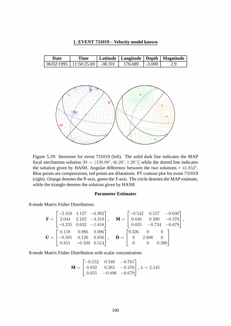
Date Time Latitude Longitude Depth Magnitude06/02/1995 11:50:25.69 -38.101 176.689 -3.000 2.9
Figure 5.29: Stereonet for event 731019 (left). The solid dark line indicates the MAPfocal mechanism solution[Θ = (130.88◦, 46.28◦, 1.28◦)] while the dotted line indicatesthe solution given by HASH. Angular difference between the two solutions =41.852◦.Blue points are compressions, red points are dilatations. PT contour plot for event 731019(right). Orange denotes the P-axis, green the T-axis. The circle denotes the MAP estimate,while the triangle denotes the solution given by HASH.
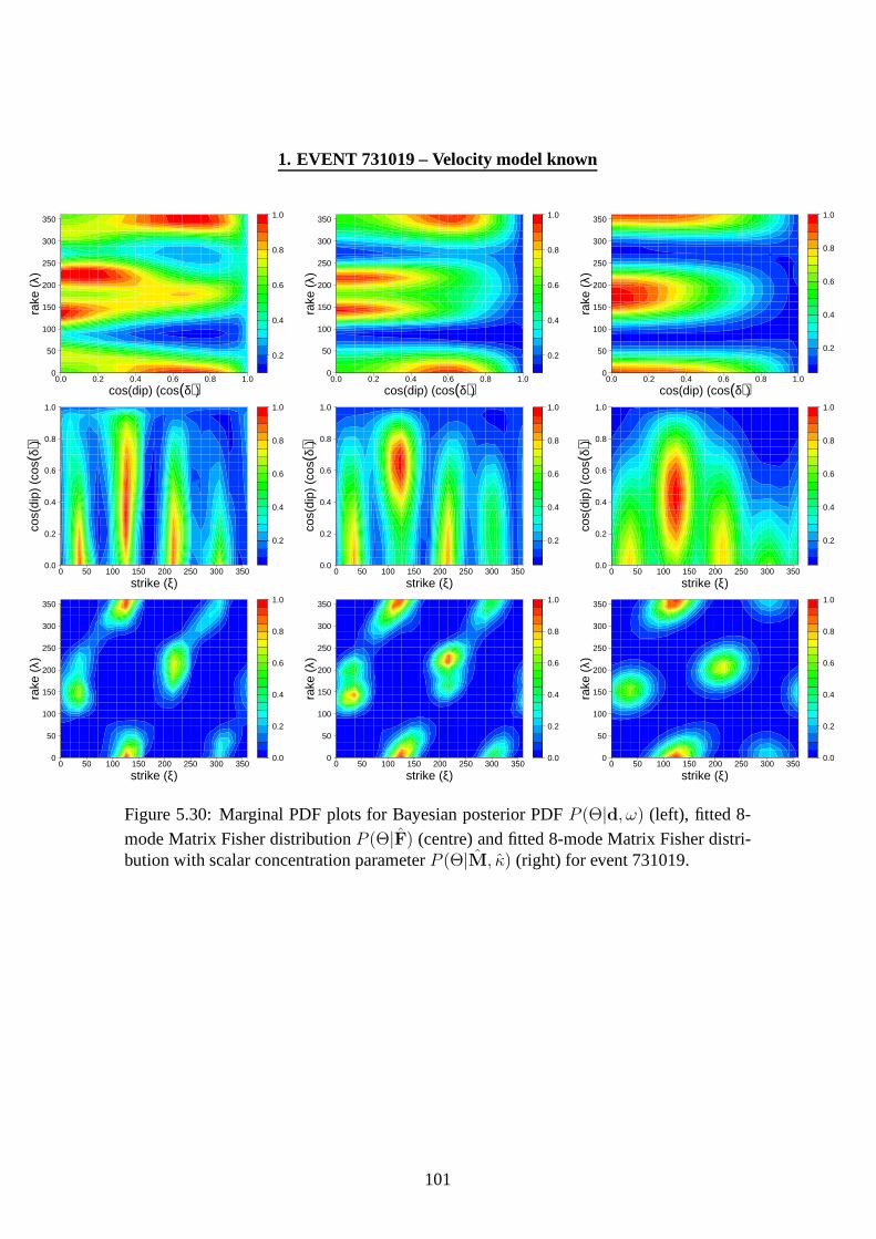
Figure 5.30: Marginal PDF plots for Bayesian posterior PDFP (Θ|d, ω) (left), fitted 8-
mode Matrix Fisher distributionP (Θ|F) (centre) and fitted 8-mode Matrix Fisher distri-bution with scalar concentration parameterP (Θ|M, κ) (right) for event 731019.
101
1. EVENT 731019 – Velocity model unknown
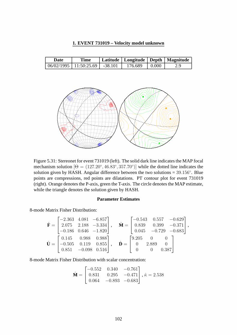
Date Time Latitude Longitude Depth Magnitude06/02/1995 11:50:25.69 -38.101 176.689 0.000 2.9
Figure 5.31: Stereonet for event 731019 (left). The solid dark line indicates the MAP focalmechanism solution[Θ = (127.20◦, 46.83◦, 357.70◦)] while the dotted line indicates thesolution given by HASH. Angular difference between the two solutions =39.156◦. Bluepoints are compressions, red points are dilatations. PT contour plot for event 731019(right). Orange denotes the P-axis, green the T-axis. The circle denotes the MAP estimate,while the triangle denotes the solution given by HASH.
Figure 5.32: Marginal PDF plots for Bayesian posterior PDFP (Θ|d, ω) (left), fitted 8-
mode Matrix Fisher distributionP (Θ|F) (centre) and fitted 8-mode Matrix Fisher distri-bution with scalar concentration parameterP (Θ|M, κ) (right) for event 731019.
103
2. EVENT 745516 – Velocity model known
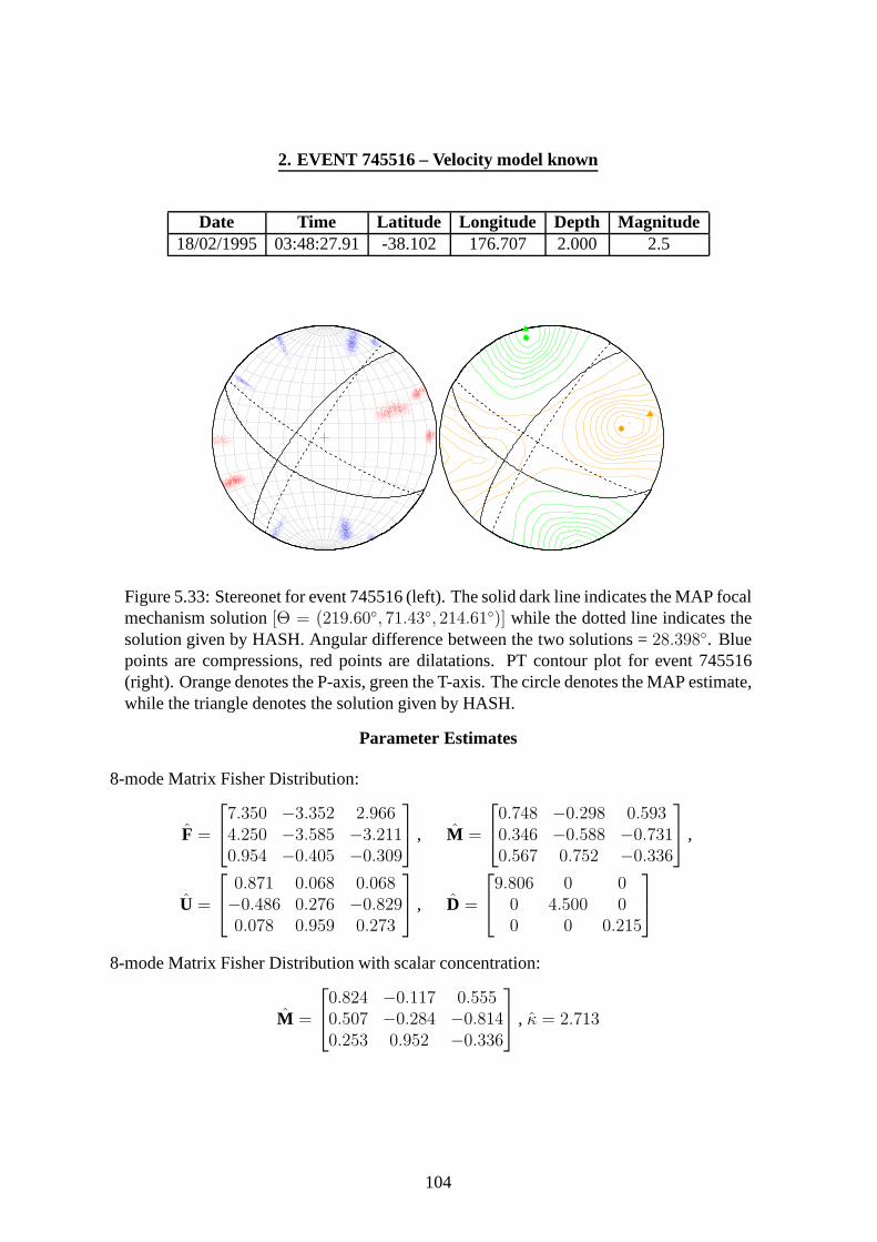
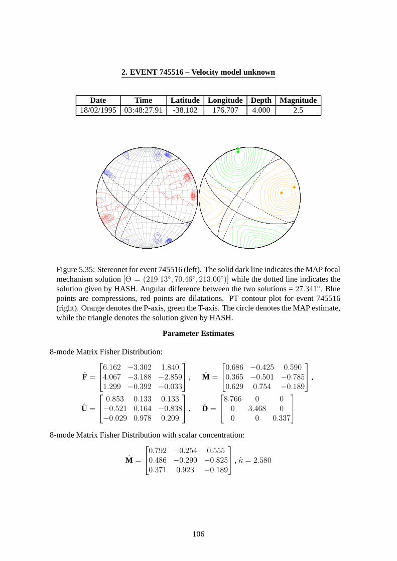
Date Time Latitude Longitude Depth Magnitude18/02/1995 03:48:27.91 -38.102 176.707 2.000 2.5
Figure 5.33: Stereonet for event 745516 (left). The solid dark line indicates the MAP focalmechanism solution[Θ = (219.60◦, 71.43◦, 214.61◦)] while the dotted line indicates thesolution given by HASH. Angular difference between the two solutions =28.398◦. Bluepoints are compressions, red points are dilatations. PT contour plot for event 745516(right). Orange denotes the P-axis, green the T-axis. The circle denotes the MAP estimate,while the triangle denotes the solution given by HASH.
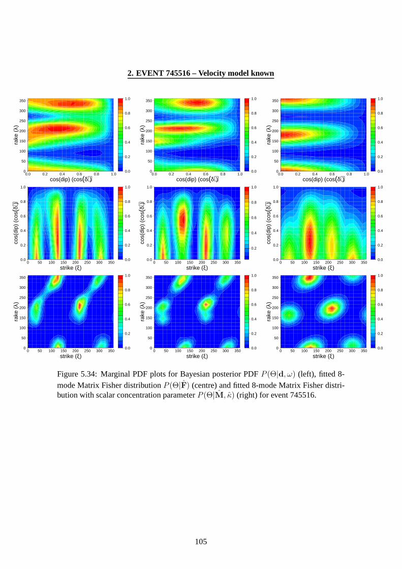
Figure 5.34: Marginal PDF plots for Bayesian posterior PDFP (Θ|d, ω) (left), fitted 8-
mode Matrix Fisher distributionP (Θ|F) (centre) and fitted 8-mode Matrix Fisher distri-bution with scalar concentration parameterP (Θ|M, κ) (right) for event 745516.
105
2. EVENT 745516 – Velocity model unknown
Date Time Latitude Longitude Depth Magnitude18/02/1995 03:48:27.91 -38.102 176.707 4.000 2.5
Figure 5.35: Stereonet for event 745516 (left). The solid dark line indicates the MAP focalmechanism solution[Θ = (219.13◦, 70.46◦, 213.00◦)] while the dotted line indicates thesolution given by HASH. Angular difference between the two solutions =27.341◦. Bluepoints are compressions, red points are dilatations. PT contour plot for event 745516(right). Orange denotes the P-axis, green the T-axis. The circle denotes the MAP estimate,while the triangle denotes the solution given by HASH.
Figure 5.36: Marginal PDF plots for Bayesian posterior PDFP (Θ|d, ω) (left), fitted 8-
mode Matrix Fisher distributionP (Θ|F) (centre) and fitted 8-mode Matrix Fisher distri-bution with scalar concentration parameterP (Θ|M, κ) (right) for event 745516.
107
3. EVENT 788921 – Velocity model known
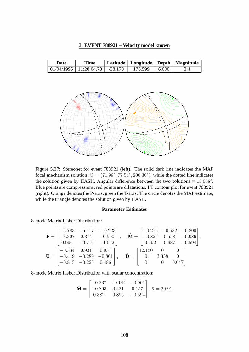
Date Time Latitude Longitude Depth Magnitude01/04/1995 11:28:04.73 -38.178 176.599 6.000 2.4
Figure 5.37: Stereonet for event 788921 (left). The solid dark line indicates the MAPfocal mechanism solution[Θ = (71.99◦, 77.54◦, 200.30◦)] while the dotted line indicatesthe solution given by HASH. Angular difference between the two solutions =15.068◦.Blue points are compressions, red points are dilatations. PT contour plot for event 788921(right). Orange denotes the P-axis, green the T-axis. The circle denotes the MAP estimate,while the triangle denotes the solution given by HASH.
Figure 5.38: Marginal PDF plots for Bayesian posterior PDFP (Θ|d, ω) (left), fitted 8-
mode Matrix Fisher distributionP (Θ|F) (centre) and fitted 8-mode Matrix Fisher distri-bution with scalar concentration parameterP (Θ|M, κ) (right) for event 788921.
109
3. EVENT 788921 – Velocity model unknown
Date Time Latitude Longitude Depth Magnitude01/04/1995 11:28:04.73 -38.178 176.599 8.000 2.4
Figure 5.39: Stereonet for event 788921 (left). The solid dark line indicates the MAP focalmechanism solution[Θ = (250.38◦, 95.81◦, 170.73◦)] while the dotted line indicates thesolution given by HASH. Angular difference between the two solutions =18.778◦. Bluepoints are compressions, red points are dilatations. PT contour plot for event 788921(right). Orange denotes the P-axis, green the T-axis. The circle denotes the MAP estimate,while the triangle denotes the solution given by HASH.