UAI 2014 Workshop Causal Inference: Learning and Prediction

Joris M. Mooij,Dominik Janzing,Jonas Peters,Tom Claassen,Antti Hyttinen (Eds.)

Proceedings of the

UAI 2014 Workshop

Causal Inference: Learning and Prediction

Quebec City, Quebec, CanadaJuly 27, 2014

c© 2014 for the individual papers by the papers’ authors. Copying permitted for private and academic purposes.Re-publication of material from this volume requires permission by the copyright owners.

Preface

We are pleased to present the Proceedings of the UAI 2014 Workshop on Causal Inference: Learning and Prediction, heldin Quebec City, Canada, on July 27, 2014, as a workshop of the 30th Conference on Uncertainty in Artificial Intelligence(UAI 2014). This workshop is the third in a series of UAI workshops on the topic of causality, following up on twosuccessful predecessors, the UAI Workshop on Causal Structure Learning 2012 and the Approaches to Causal StructureLearning Workshop, UAI 2013.

The aim of this workshop was to bring together researchers interested in the challenges of causal inference from observa-tional and interventional data, especially when confounding variables, feedback loops or selection bias may be present. Forthis workshop, we decided to extend the scope from causal structure learning to include methods for making causal predic-tions, i.e., for predicting what happens under interventions. We especially encouraged contributions describing practicalapplications of causal methods.

There were 8 submissions, all full-length papers, each of which was peer-reviewed by two or three program committeemembers. We accepted five of these for oral presentation and for inclusion in these proceedings. The proceedings alsoinclude abstracts for three invited talks, including the two key-note talks by Robert Spekkens and Elias Bareinboim. Slidesof most of the oral presentations are available on the workshop website:

https://staff.fnwi.uva.nl/j.m.mooij/uai2014-causality-workshop/index.html

We would like to thank the paper authors and presenters for their contributions and the program committee members fortheir reviewing service. We also appreciate the organizational support of the main UAI 2014 conference, in particular wewould like to thank John Mark Agosta, Jin Tian and Ann Nicholson for their help. Further, we would like to thank RobinEvans, chair of the Approaches to Causal Structure Learning Workshop, UAI 2013, for his assistance. Finally, many thanksto the CEUR-WS team for hosting these proceedings.

October 2014 Joris M. Mooij (Chair)Dominik Janzing

Jonas PetersTom ClaassenAntti Hyttinen

iii

Organizing Committee

Joris M. Mooij University of Amsterdam (Chair)Dominik Janzing Max Planck Institute for Intelligent SystemsJonas Peters ETH ZurichTom Claassen Radboud University NijmegenAntti Hyttinen California Institute of Technology

Program Committee

Thomas Richardson University of WashingtonRicardo Silva University College LondonMarkus Kalisch ETH ZurichFrederick Eberhardt California Institute of TechnologyAlain Hauser ETH ZurichIlya Shpitser University of SouthamptonRobin Evans University of OxfordKun Zhang Max Planck Institute for Intelligent SystemsEleni Sgouritsa Max Planck Institute for Intelligent SystemsAapo Hyvarinen University of HelsinkiJan Lemeire Vrije Universiteit BrusselJames Robins Harvard School of Public HealthChris Meek Microsoft ResearchPreetam Nandy ETH ZurichPhilipp Geiger Max Planck Institute for Intelligent SystemsNicholas Cornia University of AmsterdamOliver Stegle The European Bioinformatics Institute

iv

Contents

Preface iii

Full papers 1

How Occam’s Razor Provides a Neat Definition of Direct CausationAlexander Gebharter, Gerhard Schurz . . . . . . . . . . . . . . . . . . . . . . . . . . . . . . . . . . . . 1

Constructing Separators and Adjustment Sets in Ancestral GraphsBenito van der Zander, Maciej Liskiewicz, Johannes Textor . . . . . . . . . . . . . . . . . . . . . . . . . 11

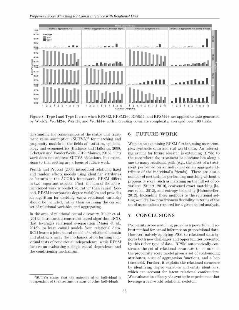
Propensity Score Matching for Causal Inference with Relational DataDavid Arbour, Katerina Marazopoulou, Dan Garant, David Jensen . . . . . . . . . . . . . . . . . . . . . 25

Type-II Errors of Independence Tests Can Lead to Arbitrarily Large Errors in Estimated Causal Effects: AnIllustrative ExampleNicholas Cornia, Joris M. Mooij . . . . . . . . . . . . . . . . . . . . . . . . . . . . . . . . . . . . . . . 35

Toward Learning Graphical and Causal Process ModelsChristopher Meek . . . . . . . . . . . . . . . . . . . . . . . . . . . . . . . . . . . . . . . . . . . . . . . 43

Abstracts 49

On Causal Explanations of Quantum CorrelationsRobert W. Spekkens . . . . . . . . . . . . . . . . . . . . . . . . . . . . . . . . . . . . . . . . . . . . . . 49

Generalizability of Causal and Statistical RelationsElias Bareinboim . . . . . . . . . . . . . . . . . . . . . . . . . . . . . . . . . . . . . . . . . . . . . . . 51

Estimating Causal Effects by Bounding ConfoundingPhilipp Geiger, Dominik Janzing, Bernhard Scholkopf . . . . . . . . . . . . . . . . . . . . . . . . . . . 53

v

vi

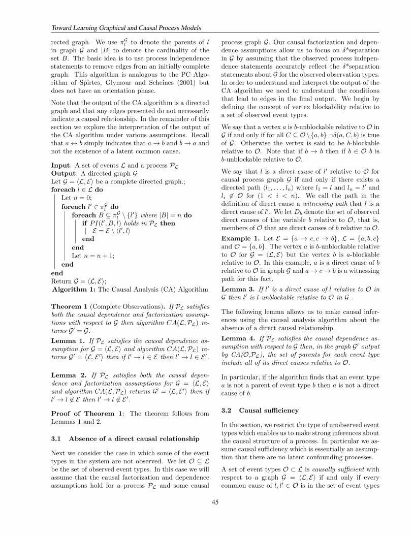
How Occam’s Razor Provides a Neat Definition of Direct Causation

Alexander Gebharter & Gerhard SchurzDuesseldorf Center for Logic and Philosophy of Science

University of DuesseldorfUniversitaetsstrasse 1

40225 Duesseldorf, Germany

Abstract

In this paper we show that the application of Oc-cam’s razor to the theory of causal Bayes netsgives us a neat definition of direct causation. Inparticular we show that Occam’s razor impliesWoodward’s (2003) definition of direct causa-tion, provided suitable intervention variables ex-ist and the causal Markov condition (CMC) issatisfied. We also show how Occam’s razor canaccount for direct causal relationships Woodwardstyle when only stochastic intervention variablesare available.

1 INTRODUCTION

Occam’s razor is typically seen as a methodological prin-ciple. There are many possible ways to apply the razor tothe theory of causal Bayes nets. It could, for example, sim-ply be interpreted to suggest preferring the simplest causalstructure compatible with the given data among all compat-ible causal structures. The simplest causal structure could,for instance, be the one (or one of the ones) featuring thefewest causal arrows.

In this paper, however, we are interested in a slightly dif-ferent application of Occam’s razor: Our interpretation ofOccam’s razor asserts that given a causal structure is com-patible with the data, it should only be chosen if it satis-fies the causal minimality condition (Min) in the sense ofSpirtes et al. (2000, p. 31), which requires that no causalarrow in the structure can be omitted in such a way that theresulting substructure would still be compatible with thedata. When speaking of a causal structure being compat-ible with the data, we have a causal structure and a prob-ability distribution satisfying the causal Markov condition(CMC) in mind. (For details, see sec. 5.) In the following,applying Occam’s razor always means to assume that thecausal minimality condition is satisfied.

In this paper we give a motivation for Occam’s razor that

goes beyond its merits as a methodological principle dic-tating that one should always decide in favor of minimalcausal models. In particular, we show that Occam’s ra-zor provides a neat definition of direct causal relatednessin the sense of Woodward (2003), provided suitable in-tervention variables exist and CMC is satisfied. Note theconnection of this enterprise to Zhang and Spirtes’ (2011)project. Zhang and Spirtes prove that CMC and an in-terventionist definition of direct causation a la Woodward(2003) together imply minimality. So Occam’s razor iswell-motivated within a manipulationist framework such asWoodward’s. We show, vice versa, that CMC and minimal-ity together imply Woodward’s definition of direct causa-tion. So if one wants a neat definition of direct causation,it is reasonable to apply Occam’s razor in the sense of as-suming minimality.

The paper is structured as follows: In sec. 2 we introducethe notation we use in subsequent sections. In sec. 3 wepresent Woodward’s (2003) definition of direct causationand his definition of an intervention variable. In sec. 4 wegive precise reconstructions of both definitions in terms ofcausal Bayes nets. We also provide a definition of the no-tion of an intervention expansion, which is needed to ac-count for direct causal relations in terms of the existence ofcertain intervention variables. In sec. 5 we show that Oc-cam’s razor gives us Woodward’s definition of direct cau-sation if CMC is assumed and the existence of suitable in-tervention variables is granted (theorem 2). In sec. 6 wego a step further and show how Occam’s razor allows usto account for direct causation Woodward style when onlystochastic intervention variables (cf. Korb et al., 2004, sec.5) are available (theorem 3). We conclude in sec. 7.

Note that though the main results of the present paper(i.e., theorems 2 and 3) can be used for causal discov-ery, the goal of this paper is not to provide a method foruncovering direct causal connections among variables ina set of variables V of interest. The goal of this paperis to establish a connection between Woodward’s (2003)intervention-based notion of direct causation and the pres-ence of a causal arrow in a minimal causal Bayes net, which

1

can be interpreted as support for Occam’s razor. Because ofthis, the present paper does not discuss the relation of theo-rems 2 and 3 to results about causal discovery by means ofinterventions such as, e.g., (Eberhardt and Scheines, 2007)or (Nyberg and Korb, 2007).

2 NOTATION

We represent causal structures by graphs, i.e., by orderedpairs 〈V, E〉, where V is a set of variables andE is a binaryrelation on V (E ⊆ V ×V). V’s elements are called thegraph’s “vertices” and E’s elements are called its “edges”.“X → Y ” stands short for “〈X,Y 〉 ∈ E” and is interpretedas “X is a direct cause of Y in 〈V, E〉” or as “Y is a directeffect of X in 〈V, E〉”. Par(Y ) is the set of all X ∈ Vwith X → Y in 〈V, E〉. The elements of Par(Y ) arecalled Y ’s parents. We write “X – Y ” for “X → Y orX ← Y ”. A path π : X – ... – Y is called a (causal)path connecting X and Y in 〈V, E〉. A causal path π iscalled a directed causal path from X to Y if and only if(“iff” for short) it has the form X → ... → Y . X is calleda cause of Y and Y an effect of X in that case. A causalpath π is called a common cause path iff it has the formX ← ... ← Z → ... → Y and no variable appears moreoften than once on π. Z is called a common cause of Xand Y lying on path π in that case. A variable Z lying on apath π : X – ... → Z ← ... – Y is called a collider lyingon this path. A variable X is called exogenous iff no arrowis pointing at X; it is called endogenous otherwise.

A graph 〈V, E〉 is called a directed graph in case all edgesin E are one-headed arrows “→”. It is called cyclic iffit features a causal path of the form X → ... → X andacyclic otherwise. A causal structure 〈V, E〉 together witha probability distribution P over V is called a causal model〈V, E, P 〉. P is intended to provide information about thestrengths of causal influences represented by the arrows in〈V, E〉. A causal model 〈V, E, P 〉 is called cyclic iff itsgraph 〈V, E〉 is cyclic; it is called acyclic otherwise. Inthe following, we will only be interested in acyclic causalmodels.

We use the standard notions of (conditional) probabilisticdependence and independence:

Definition 1 (conditional probabilistic (in)dependence)X and Y are probabilistically dependent conditional on Ziff there are X-, Y -, and Z-values x, y, and z, respectively,such that P (x|y, z) 6= P (x|z) ∧ P (y, z) > 0.

X and Y are probabilistically independent conditional onZ iff X and Y are not probabilistically dependent condi-tional on Z.

Probabilistic independence between X and Y conditionalon Z is abbreviated as “Indep(X,Y |Z)”, probabilisticdependence is abbreviated as “Dep(X,Y |Z)”. Uncon-

ditional probabilistic (in)dependence between X and Y(In)Dep(X,Y ) is defined as (In)Dep(X,Y |∅). X , Y ,and Z in definition 1 can be variables or sequences ofvariables. When X,Y, Z, ... are sequences of variables,we write them in bold letters. We write also the valuesx,y, z, ... of sequences X,Y,Z, ... in bold letters. Theset of values x of a sequence X of variables X1, ..., Xn

is val(X1) × ... × val(Xn), where val(Xi) is the set ofXi’s possible values.

3 WOODWARD’S DEFINITION OFDIRECT CAUSATION

Woodward’s (2003) interventionist theory of causationaims to explicate direct causation w.r.t. a set of variablesV in terms of possible interventions. Woodward (2003,p. 98) provides the following definition of an interventionvariable:

Definition 2 (IVW ) I is an intervention variable for Xwith respect to Y if and only if I meets the following con-ditions:I1. I causes X .I2. I acts as a switch for all the other variables that causeX . That is, certain values of I are such that when I attainsthose values, X ceases to depend on the values of othervariables that cause X and instead depends only on thevalue taken by I .I3. Any directed path from I to Y [if there exists one] goesthrough X [...].I4. I is (statistically) independent of any variable Z thatcauses Y and that is on a directed path that does not gothrough X .

(IVW ) is intended to single out those variables as interven-tion variables for X w.r.t. Y that allow for correct causalinference according to Woodward’s (2003) definition of di-rect causation. For I to be an intervention variable for Xw.r.t. Y it is required that I is causally relevant to X (con-dition I1), that X is only under I’s influence when I = on(condition I2), and that a correlation between I and Y canonly be due to a directed causal path from I to Y goingthroughX (conditions I3 and I4). For a detailed motivationof I1-I4, see (Woodward, 2003, sec. 3.1.4). For problemswith Woodward’s definitions, see (Gebharter and Schurz,ms).

An intervention on X w.r.t. Y (from now on we refer to Xas the intervention’s “target variable” and to Y as the “testvariable”) is then straightforwardly defined as an interven-tion variable I for X w.r.t. Y taking one of its on-values,which forces X to take a certain value x. We will call in-terventions whose on-values force X to take certain valuesx “deterministic interventions” (cf. Korb et al., 2004, sec.5).


2

Note that Woodward’s (2003) notion of an intervention is,on the one hand, strong because it requires interventionsto be deterministic interventions. It is, on the other hand,weak in another respect: In contrast to structural or surgi-cal interventions (cf. Eberhardt and Scheines, 2007, p. 984;Pearl, 2009) Woodward’s interventions are allowed to bedirect causes of more than one variable as long as the in-tervention’s direct effects which are non-target variables donot cause the test variable over a path not going through theintervention’s target variable (intervention condition I3).

Based on his notion of an intervention, Woodward (2003, p.59) gives the following definition of direct causation w.r.t.a variable set V:

Definition 3 (DCW ) A necessary and sufficient conditionfor X to be a (type-level) direct cause of Y with respect toa variable set V is that there be a possible intervention onX that will change Y or the probability distribution of Ywhen one holds fixed at some value all other variables Zi

in V.

(DCW ) neatly explicates direct causation w.r.t. a variableset V in terms of possible interventions: X is a direct causeof Y w.r.t. V if Y can be wiggled by wiggling X; and ifX is a direct cause of Y w.r.t. V, then there are possibleinterventions by whose means one can influence Y by ma-nipulating X .1

Note that (DCW ) may be too strong because many domainsinvolve variables one cannot control by deterministic inter-ventions. Scenarios of this kind include, for example, thedecay of uranium or states of entangled systems in quantummechanics. The decay of uranium can only be probabilis-tically influenced, and any attempt to manipulate the stateof one of two entangled photons, for example, would de-stroy the entangled system. Glymour (2004) also considersvariables for sex and race as not manipulable by means ofintervention variables in the sense of (IVW ).

To avoid all problems that might arise for Woodward’s(2003) account due to variables that are not manipulableby deterministic interventions, we will reconstruct Wood-ward’s (DCW ) as a partial definition in sec. 4. In particular,we will define direct causation only for sets of variables Vfor which suitable intervention variables exist.

4 RECONSTRUCTING WOODWARD’SDEFINITION

In this section we reconstruct Woodward’s (2003) defini-tion of direct causation in terms of causal Bayes nets. Thereconstruction of (IVW ) is straightforward:

1Note that Woodward (2003) does not require the interventionvariables I to be elements of the set of variables V containing thetarget variable X and the test variable Y .

Definition 4 (IV) IX ∈ V is an intervention variable forX ∈ V w.r.t. Y ∈ V in a causal model 〈V, E, P 〉 iff(a) IX is exogenous and there is a path π : IX → X in〈V, E〉,(b) for every on-value of IX there is an X-value x suchthat P (x|IX = on) = 1 and Dep(x, IX = on|z) holds forevery instantiation z of every Z ⊆ V\{IX , X},(c) all paths IX → ...→ Y in 〈V, E〉 have the form IX →...→ X → ...→ Y ,(d) IX is independent from every variable C (in V or notin V) which causes Y over a path not going through X .

Note that (IV) still allows for intervention variables IX thatare common causes of their target variable X and othervariables in V. Condition (a) requires IX to be exogenous.This is, though it is a typical assumption made for interven-tion variables, not explicit in Woodward’s (2003) originaldefinition (IVW ). One problem that might arise for Wood-ward’s account when not making this assumption is that IXin a causal structure Y → IX → X may turn out to be anintervention variable for X w.r.t. Y . If Y then depends onIX = on, (DCW ) would falsely determine X to be a causeof Y (cf. Gebharter and Schurz, ms). IX → X in condi-tion (a) is a harmless simplification of I1. Condition (b)captures Woodward’s requirement that interventions haveto be deterministic, from which I2 follows. X is assumedto be under full control of IX when IX is on. This doesnot only require that for every on-value of IX there is anX-value x such that P (x|IX = on) = 1, but also thatIX = on actually has an influence on x in every possiblecontext, i.e., under conditionalization on arbitrary instanti-ations z of all kinds of subsets Z of V\{IX , X}. Condition(c) directly mirrors I3. Condition (d) mirrors Woodward’sI4. Note that condition (d) requires reference to variablesCpossibly not contained in V (cf. Woodward, 2008, p. 202).

If we want to account for direct causal connection in acausal model 〈V, E, P 〉 by means of interventions, wehave to add intervention variables to V. In other words:We have to expand 〈V, E, P 〉 in a certain way. But howdo we have to expand 〈V, E, P 〉? To answer this question,let us assume that we want to know whether X is a directcause of Y in the unmanipulated model 〈V, E, P 〉. Thenthe manipulated model 〈V′, E′, P ′〉 will have to contain anintervention variable IX for X w.r.t. Y and also interven-tion variables IZ for all Z ∈ V different from X and Y bywhose means these Z can be controlled. X is a direct causeof Y if IX has some on-values such that we can influence Yby manipulating X with IX = on when all IZ have takencertain on-values. On the other hand, to guarantee that Xis not a direct cause of Y , we have to demonstrate that noone of Y ’s values can be influenced by manipulating someX-value by some intervention. For establishing such a neg-ative causal claim, we require an intervention variable IXby whose means we can control every X-value x. (Oth-erwise it could be that Y depends only on X-values that


3

are not correlated with IX -values; then IX = on wouldhave no probabilistic influence on Y , though X may bea causal parent of Y .) In addition, we require for everyZ 6= X,Y an intervention variable IZ by whose means Zcan be forced to take every value z. (Otherwise it couldbe that we can bring about only such Z-value instantia-tions which screen X and Y off each other; then IX = onwould have no probabilistic influence on Y when Z’s valueis fixed by interventions, though X may be a causal parentof Y .)

In the unmanipulated model 〈V, E, P 〉, all interven-tion variables I are off . In the manipulated model〈V′, E′, P ′〉, all intervention variables’ values are realizedfor some but not for all individuals in the domain. Thismove allows us to compute probabilities for variables in Vwhen I = off as well as probabilities for variables in Vfor all combinations of on-value realizations of interven-tion variables I , while the causal structure of the unmanip-ulated model will be preserved in the manipulated model.(Note that we deviate here from the typical “arrow break-ing” representation of interventions in the literature whichassumes that in the manipulated model all individuals getmanipulated.) This amounts to the following notion of anintervention expansion (“i-expansion” for short):

Definition 5 (intervention expansion) 〈V′, E′, P ′〉 is anintervention expansion of 〈V, E, P 〉 w.r.t. Y ∈ V iff(a) V′ = V∪VI, where VI contains for every X ∈ Vdifferent from Y an intervention variable IX w.r.t. Y (andnothing else),(b) for all Zi, Zj ∈ V : Zi → Zj in E′ iff Zi → Zj in E,(c) for every X-value x of every X ∈ V different fromY there is an on-value of the corresponding interven-tion variable IX such that P ′(x|IX = on) = 1 andDep(x, IX = on|z) holds for every instantiation z of everyZ ⊆ V\{IX , X},(d) P ′I=off ↑ V = P ,(e) P ′(I = on), P ′(I = off) > 0.

I in conditions (d) and (e) is the set of all newly added in-tervention variables I . P ′I=off ↑ V in (d) is P ′I=off :=P ′(−|I = off) restricted to V. Hence, “P ′I=off ↑ V = P ”means that P ′I=off coincides with P on the value spaceof variables in V. Condition (a) guarantees that the i-expansion contains all the intervention variables requiredfor testing for direct causal relationships in the sense ofWoodward’s (2003) definition of direct causation. The as-sumption that VI contains only intervention variables forX w.r.t. Y is a harmless simplification. Thanks to condi-tion (b), the manipulated model’s causal structure fits to theunmanipulated model’s causal structure. In particular, thei-expansion is only allowed to introduce new causal arrowsgoing from intervention variables to variables in V. Dueto condition (c), every X ∈ V different from Y can befully controlled by means of an intervention variable IX

for X w.r.t. Y . Condition (d) explains how the manipu-lated model’s associated probability distribution P ′ fits tothe unmanipulated model’s distribution P . Condition (e)says that all values of intervention variables have to be re-alized by some individuals in the domain.

With help of this notion of an i-expansion we can now re-construct Woodward’s (2003) definition of direct causation.As already mentioned, Woodward’s definition requires theexistence of suitable intervention variables. Thus, we re-construct (DCW ) as a partial definition whose if-conditionpresupposes the required intervention variables:

Definition 6 (DC) If there exist i-expansions 〈V′, E′, P ′〉of 〈V, E, P 〉 w.r.t. Y ∈ V, then: X ∈ V is a directcause of Y w.r.t. V iff Dep(Y, IX = on|IZ = on) holdsin some i-expansions 〈V′, E′, P ′〉 of 〈V, E, P 〉 w.r.t. Y ,where IX is an intervention variable for X w.r.t. Y in〈V′, E′, P ′〉 and IZ is the set of all intervention variablesin 〈V′, E′, P ′〉 different from IX .

(DC) mirrors Woodward’s definition restricted to cases inwhich the required intervention variables (more precisely:the required i-expansions) exist: In case Y can be proba-bilistically influenced by manipulating X by means of anintervention variable IX for X w.r.t. Y in one of these i-expansions, X is a direct cause of Y in the unmanipulatedmodel. And vice versa: In case X is a direct cause of Yin the unmanipulated model, there will be an interventionvariable IX forX w.r.t. Y in one of these i-expansions suchthat Y is probabilistically sensitive to IX = on.

In the next section we show that (DC) can account for alldirect causal dependencies in a causal model if suitable i-expansions exist and CMC and Min are assumed to be sat-isfied.

5 OCCAM’S RAZOR, DETERMINISTICINTERVENTIONS, AND DIRECTCAUSATION

The theory of causal Bayes nets’ core axiom is the causalMarkov condition (CMC) (cf. Spirtes et al., 2000, p. 29):

Definition 7 (causal Markov condition) A causal model〈V, E, P 〉 satisfies the causal Markov condition iff everyX ∈ V is probabilistically independent of all its non-effects conditional on its causal parents.

CMC is assumed to hold for causal models whose variablesets are causally sufficient. A variable set V is causally suf-ficient iff every common cause C of variables X and Y inV is also in V or takes the same value c for all individualsin the domain (cf. Spirtes et al., 2000, p. 22). From now onwe implicitly assume causal sufficiency, i.e., we only con-sider causal models whose variable sets are causally suffi-cient.


4

A finite causal model 〈V, E, P 〉 satisfies the Markov con-dition iff P admits the following Markov factorization rel-ative to 〈V, E〉 (cf. Pearl, 2009, p. 16):

P (X1, ..., Xn) =∏

i

P (Xi|Par(Xi)) (1)

The conditional probabilities P (Xi|Par(Xi)) are calledXi’s parameters.

For acyclic causal models, CMC is equivalent to the d-separation criterion (Verma, 1986; Pearl, 1988, pp. 119f):

Definition 8 (d-separation criterion) 〈V, E, P 〉 satisfiesthe d-separation criterion iff the following holds for allX,Y ∈ V and Z ⊆ V\{X,Y }: If X and Y are d-separated by Z in 〈V, E〉, then Indep(X,Y |Z).

Definition 9 (d-separation, d-connection) X ∈ V andY ∈ V are d-separated by Z ⊆ V\{X,Y } in 〈V, E〉 iffX and Y are not d-connected given Z in 〈V, E〉.X ∈ V and Y ∈ V are d-connected given Z ⊆ V\{X,Y }in 〈V, E〉 iffX and Y are connected by a path π in 〈V, E〉such that no non-collider on π is in Z, while all colliderson π are in Z or have an effect in Z.

The equivalence between CMC and the d-separation cri-terion reveals the full content of CMC: If a causal modelsatisfies CMC, then every (conditional) probabilistic inde-pendence can be explained by missing (conditional) causalconnections, and every (conditional) probabilistic depen-dence can be explained by some existing (conditional)causal connection.

In case there is a path π between X and Y in 〈V, E〉 suchthat no non-collider on π is in Z ⊆ V\{X,Y } and all col-liders on π are in Z or have an effect in Z, π is said to beactivated by Z. We also say that X and Y are d-connectedgiven Z over path π in that case. If π is not activated by Z,π is said to be blocked by Z. We also say that X and Y ared-separated by Z over path π in that case.

Occam’s razor (as we understand it in this paper) dictatesto prefer from all those causal structures 〈V, E〉, which to-gether with a given probability distribution P over V sat-isfy CMC, the ones which also satisfy the causal minimal-ity condition (Min):

Definition 10 (causal minimality condition) A causalmodel 〈V, E, P 〉 satisfying CMC satisfies the causalminimality condition iff no model 〈V, E′, P 〉 with E′ ⊂ Ealso satisfies CMC (cf. Spirtes et al., 2000, p. 31).

For acyclic causal models satisfying CMC, the followingcausal productivity condition (Prod) (cf. Schurz and Geb-harter, forthcoming) can be seen as a reformulation of thecausal minimality condition:

Definition 11 (causal productivity condition) A causalmodel 〈V, E, P 〉 satisfies the causal productivity conditioniff Dep(X,Y |Par(Y )\{X}) holds for all X,Y ∈ V withX → Y in 〈V, E〉.

Theorem 1 For every acyclic causal model 〈V, E, P 〉 sat-isfying CMC, the causal minimality condition and thecausal productivity condition are equivalent.

The equivalence of Min and Prod reveals the full content ofMin: In minimal causal models, no causal arrow is super-fluous, i.e., every causal arrow from X to Y is productive,meaning that it is responsible for some probabilistic depen-dence between X and Y (when the values of all other par-ents of Y are fixed).

We can now prove the following theorem:

Theorem 2 If 〈V, E, P 〉 is an acyclic causal model andfor every Y ∈ V there is an i-expansion 〈V′, E′, P ′〉 of〈V, E, P 〉 w.r.t. Y satisfying CMC and Min, then for allX,Y ∈ V (with X 6= Y ) the following two statements areequivalent:(i) X → Y in 〈V, E〉.(ii)Dep(Y, IX = on|IZ = on) holds in some i-expansions〈V′, E′, P ′〉 of 〈V, E, P 〉w.r.t. Y , where IX is an interven-tion variable forX w.r.t. Y in 〈V′, E′, P ′〉 and IZ is the setof all intervention variables in 〈V′, E′, P ′〉 different fromIX .

Theorem 2 shows that direct causation a la Woodward(2003) coincides with the graph theoretical notion of directcausation in systems 〈V, E, P 〉 with i-expansions w.r.t. ev-ery variable Y ∈ V satisfying CMC and Min. In particular,theorem 2 says the following: Assume we are interested ina causal model 〈V, E, P 〉. Assume further that for everyY in V there is an i-expansion 〈V′, E′, P ′〉 of 〈V, E, P 〉w.r.t. Y satisfying CMC and Min. This means (amongother things) that for every pair of variables 〈X,Y 〉 there isat least one i-expansion with an intervention variable IX forX w.r.t. Y and intervention variables IZ for every Z ∈ V(different from X and Y ) w.r.t. Y by whose means one canforce the variables in V\{Y } to take any combination ofvalue realizations. Given this setup, theorem 2 tells us forevery X and Y (with X 6= Y ) in V that X is a causal par-ent of Y in 〈V, E〉 iff Dep(Y, IX = on|IZ = on) holds inone of the presupposed i-expansions w.r.t. Y .

6 OCCAM’S RAZOR, STOCHASTICINTERVENTIONS, AND DIRECTCAUSATION

In this section we generalize the main finding of sec. 5 tocases in which only stochastic interventions are available.To account for direct causal relations X → Y by meansof stochastic intervention variables, two intervention vari-


5

ables are needed, one for X and one for Y . (For details,see below.) We define a stochastic intervention variable asfollows:

Definition 12 (IVS) IX ∈ V is a stochastic interventionvariable for X ∈ V w.r.t. Y ∈ V in 〈V, E, P 〉 iff(a) IX is exogenous and there is a path π : IX → X in〈V, E〉,(b) for every on-value of IX there is an X-value x suchthat Dep(x, IX = on|z) holds for every instantiation z ofevery Z ⊆ V\{IX , X},(c) all paths IX → ...→ Y in 〈V, E〉 have the form IX →...→ X → ...→ Y ,(d) IX is independent from every variable C (in V or notin V) which causes Y over a path not going through X .

The only difference between (IVS) and (IV) is condition(b). For stochastic interventions it is not required thatIX = on determines X’s value to be x with probability1. It suffices that IX = on and x are correlated conditionalon every value z of every Z ⊆ V\{IX , X}. This specificconstraint guarantees thatX can be influenced by IX = onunder all circumstances, i.e., under all kinds of condition-alization on instantiations of remainder variables in V.

We do also have to modify our notion of an intervention ex-pansion in case we allow for stochastic interventions. Wedefine the following notion of a stochastic intervention ex-pansion:

Definition 13 (stochastic intervention expansion)〈V′, E′, P ′〉 is a stochastic intervention expansion of〈V, E, P 〉 for X ∈ V w.r.t. Y ∈ V iff(a) V′ = V∪VI, where VI contains one stochasticintervention variable IX for X w.r.t. Y and one stochasticintervention variable IY for Y w.r.t. Y which is a parentonly of Y (and nothing else),(b) for all Zi, Zj ∈ V : Zi → Zj in E′ iff Zi → Zj in E,(c.1) for every X-value x there is an on-value of IX suchthat Dep(x, IX = on|z) holds for every instantiation z ofevery Z ⊆ V′\{IX , X},(c.2) for every Y -value y, every instantiation r of Par(Y ),and every on-value of IY there is an on-value on∗ ofIY such that P ′(y|IY = on∗, r) 6= P ′(y|IY = on, r),P ′(y|IY = on∗, r) > 0, and P ′(y|IY = on∗, r∗) =P ′(y|IY = on, r∗) holds for all r∗ ∈ val(Par(Y ))different from r,(d) P ′I=off ↑ V = P ,(e) P ′(I = on), P ′(I = off) > 0.

This definition differs from the definition of a (non-stochastic) i-expansion with respect to conditions (a) and(c): A stochastic i-expansion for X w.r.t. Y contains ex-actly two intervention variables, viz. one stochastic inter-vention variable IX for X w.r.t. Y and one stochastic inter-vention variable IY for Y w.r.t. Y (which trivially satisfiesconditions (c) and (d) in (IVS)). While IX may have more

than one direct effect, the second intervention variable IYis assumed to be a causal parent only of Y . (This is requiredfor accounting for direct causal connections; for details see(i)⇒ (ii) in the proof of theorem 3 in the appendix.)

The second intervention variable IY is required to excludeindependence between IX and Y due to a fine-tuning ofY ’s parameters. Such an independence can arise even ifCMC and Min are satisfied, X is a causal parent of Y ,and IX and Y are each correlated with the same X-valuesx. For examples of this kind of non-faithfulness, see, e.g.,(Neapolitan, 2004, p. 96) or (Naeger, forthcoming). In con-dition (c.2) we assume that every one of Y ’s parameters canbe changed independently of all other Y -parameters (to avalue r ∈ ]0, 1]) by changing IY ’s on-value. This sufficesto exclude non-faithful independencies between IX and Yof the kind described above.

When not presupposing deterministic interventions, it can-not be guaranteed anymore that the value of every vari-able in our model of interest different from the test variableY can be fixed by interventions. The values of a causalmodel’s variables can, however, also be fixed by condition-alization. To account for direct causation between X andY when only stochastic interventions are available, one hasto conditionalize on a suitably chosen set Z ⊆ V\{X,Y }that (i) blocks all indirect causal paths between X and Y ,and that (ii) fixes all X-alternative parents of Y . That Zblocks all indirect paths between X and Y is required toassure that dependence between IX = on and Y cannot bedue to an indirect path, and fixing the values of all parentsof Y different from X is required to exclude independenceof IX = on and Y due to a fine-tuning of Y ’sX-alternativeparents that may cancel the influence of IX = on on Y overa path IX → X → Y .2 Fortunately, every directed acyclicgraph 〈V, E〉 features a set Z satisfying requirement (i),viz. Par(Y )\{X} (cf. Schurz and Gebharter, forthcom-ing). Trivially, Par(Y )\{X} also satisfies requirement(ii).

With the help of (IVS) and definition 13, we can now de-fine direct causation in terms of stochastic interventions formodels for which suitable stochastic i-expansions exist:

Definition 14 (DCS) If there exist stochastic i-expansions〈V′, E′, P ′〉 of 〈V, E, P 〉 for X w.r.t. Y , then: Xis a direct cause of Y w.r.t. V iff Dep(Y, IX =on|Par(Y )\{X}, IY = on) holds in some i-expansions〈V′, E′, P ′〉 of 〈V, E, P 〉 for X w.r.t. Y , where IXis a stochastic intervention variable for X w.r.t. Y in〈V′, E′, P ′〉 and IY is a stochastic intervention variablefor Y w.r.t. Y in 〈V′, E′, P ′〉.

Now the following theorem can be proven:

2For details on such cases of non-faithfulness due to com-pensating parents see (Schurz and Gebharter, forthcoming; Pearl,1988, p. 256).


6

Theorem 3 If 〈V, E, P 〉 is an acyclic causal model andfor every X,Y ∈ V (with X 6= Y ) there is a stochastici-expansion 〈V′, E′, P ′〉 of 〈V, E, P 〉 for X w.r.t. Y satis-fying CMC and Min, then for all X,Y ∈ V (with X 6= Y )the following two statements are equivalent:(i) X → Y in 〈V, E〉.(ii) Dep(Y, IX = on|Par(Y )\{X}, IY = on) holds insome i-expansions 〈V′, E′, P ′〉 of 〈V, E, P 〉 for X w.r.t.Y , where IX is a stochastic intervention variable for Xw.r.t. Y in 〈V′, E′, P ′〉 and IY is a stochastic interventionvariable for Y w.r.t. Y in 〈V′, E′, P ′〉.

Theorem 3 shows that direct causation a la Woodward(2003) coincides with the graph theoretical notion of di-rect causation in systems 〈V, E, P 〉 with stochastic i-expansions for every X ∈ V w.r.t. every Y ∈ V (withX 6= Y ) satisfying CMC and Min. In particular, theo-rem 3 says the following: Assume we are interested ina causal model 〈V, E, P 〉. Assume further that for everyX,Y in V (with X 6= Y ) there is a stochastic i-expansion〈V′, E′, P ′〉 of 〈V, E, P 〉 for X w.r.t. Y satisfying CMCand Min. This means (among other things) that for everypair of variables 〈X,Y 〉 there is at least one stochastic i-expansion featuring a stochastic intervention variable IXfor X w.r.t. Y and a stochastic intervention variable IY forY w.r.t. Y . Given this setup, theorem 3 can account for ev-ery causal arrow between every X and Y (with X 6= Y )in V: It says that X is a causal parent of Y in 〈V, E〉 iffDep(Y, IX = on|Par(Y )\{X}, IY = on) holds in someof the presupposed stochastic i-expansions for X w.r.t. Y .

7 CONCLUSION

In this paper we investigated the consequences of assuminga certain version of Occam’s razor. If one applies the razorin such a way to the theory of causal Bayes nets that it dic-tates to prefer only minimal causal models, one can showthat Occam’s razor provides a neat definition of direct cau-sation. In particular, we demonstrated that one gets Wood-ward’s (2003) definition of direct causation translated intocausal Bayes nets terminology and restricted to contexts inwhich suitable i-expansions satisfying the causal Markovcondition (CMC) exist. In the last section we showed howOccam’s razor can be used to account for direct causalconnections Woodward style even if no deterministic in-terventions are available. These results can be seen as amotivation of Occam’s razor going beyond its merits as amethodological principle: If one wants a nice and simpleinterventionist definition of direct causation in the sense ofWoodward (or its stochastic counterpart developed in sec.6), then it is reasonable to apply a version of Occam’s razorthat suggests to eliminate non-minimal causal models.

Acknowledgements

This work was supported by DFG, research unit “Causa-tion, Laws, Dispositions, Explanation” (FOR 1063). Ourthanks go to Frederick Eberhardt and Paul Naeger for im-portant discussions, to two anonymous referees for helpfulcomments on an earlier version of the paper, and to Sebas-tian Maaß for proofreading.

References

F. Eberhardt, and R. Scheines (2007). Interventions andcausal inference. Philosophy of Science 74(5):981-995.

A. Gebharter, and G. Schurz (ms). Woodward’s interven-tionist theory of causation: Problems and proposed solu-tions.

C. Glymour (2004). Critical notice. British Journal for thePhilosophy of Science 55(4):779-790.

K. B. Korb, L. R. Hope, A. E. Nicholson, and K. Axnick(2004). Varieties of causal intervention. In C. Zhang, H. W.Guesgen, W.-K. Yeap (eds.), Proceedings of the 8th PacificRim International Conference on AI 2004: Trends in Arti-ficial Intelligence, 322-331. Berlin: Springer.

P. Naeger (forthcoming). The causal problem of entangle-ment. Synthese.

R. Neapolitan (2004). Learning Bayesian Networks. UpperSaddle River, NJ: Prentice Hall.

E. P. Nyberg, and K. B. Korb (2006). Informative interven-tions. Technical report 2006/204, Clayton School of Infor-mation Technology, Monash University, Melbourne.

J. Pearl (1988). Probabilistic Reasoning in Expert Systems.San Mateo, MA: Morgan Kaufmann.

J. Pearl (2009). Causality. Cambridge: Cambridge Univer-sity Press.

G. Schurz, and A. Gebharter (forthcoming). Causality asa theoretical concept: Explanatory warrant and empiricalcontent of the theory of causal nets. Synthese.

P. Spirtes, C. Glymour, and R. Scheines (2000). Causation,Prediction, and Search. Cambridge, MA: MIT Press.

T. S. Verma (1986). Causal networks: Semantics and ex-pressiveness. Technical report R-65, Cognitive SystemsLaboratory, University of California, Los Angeles.

J. Woodward (2003). Making Things Happen. Oxford: Ox-ford University Press.

J. Woodward (2008). Response to Strevens. Philosophyand Phenomenological Research 77(1):193-212.

J. Zhang, and P. Spirtes (2011). Intervention, determinism,and the causal minimality condition. Synthese 182(3):335-347.


7

Appendix

The following proof of theorem 1 rests on the equivalenceof CMC and the Markov factorization (1). It is, thus, re-stricted to finite causal structures.

Proof of theorem 1 Suppose 〈V, E, P 〉 with V ={X1, ..., Xn} to be a finite acyclic causal model satisfyingCMC.

Prod⇒Min: Assume that 〈V, E, P 〉 does not satisfy Min,meaning that there are X,Y ∈ V with X → Y in 〈V, E〉such that 〈V, E′, P 〉, which results from deleting X → Yfrom 〈V, E〉, still satisfies CMC. But then Par(Y )\{X}d-separates X and Y in 〈V, E′〉, and thus, the d-separationcriterion implies Indep(X,Y |Par(Y )\{X}), which vio-lates Prod.

Min⇒ Prod: Assume that 〈V, E, P 〉 satisfies Min, mean-ing that there are no X,Y ∈ V with X → Y in 〈V, E〉such that 〈V, E′, P 〉, which results from deleting X → Yfrom 〈V, E〉, still satisfies CMC. The latter is the caseiff (*) the parent set Par(Y ) of every Y ∈ V (withPar(Y ) 6= ∅) is minimal in the sense that removing oneof Y ’s parents X from Par(Y ) would make a differ-ence for Y , meaning that P (y|x, Par(Y )\{X} = r) 6=P (y|Par(Y )\{X} = r) holds for some X-values x, someY -values y, and some instantiations r of Par(Y )\{X}.Otherwise P would admit the Markov factorization rela-tive to 〈V, E〉 and relative to 〈V, E′〉, meaning that also〈V, E′, P 〉, which results from deleting X → Y from〈V, E〉, would satisfy CMC. But then 〈V, E, P 〉 wouldnot be minimal, which would contradict the assumption.Now (*) entails that Dep(X,Y |Par(Y )\{X}) holds forall X,Y ∈ V with X → Y , i.e., that 〈V, E, P 〉 satisfiesProd. �

Proof of theorem 2 Assume 〈V, E, P 〉 is an acycliccausal model and for every Y ∈ V there is an i-expansion〈V′, E′, P ′〉 of 〈V, E, P 〉 w.r.t. Y satisfying CMC andMin. Let X and Y be arbitrarily chosen elements of Vsuch that X 6= Y .

(i)⇒ (ii): Suppose X → Y in 〈V, E〉. We assumed thatthere exists an i-expansion 〈V′, E′, P ′〉 of 〈V, E, P 〉 w.r.t.Y satisfying CMC and Min. From condition (b) of defi-nition 5 it follows that X → Y in 〈V′, E′〉. Since Minis equivalent to Prod, X and Y are dependent when thevalues of all parents of Y different from X are fixed tocertain values, meaning that there will be an X-value xand a Y -value y such that Dep(x, y|Par(Y )\{X} = r)holds for an instantiation r of Par(Y )\{X}. Now therewill also be a value of IZ that fixes the set of all parents ofY different from X to r. Let on be this IZ-value. Thus,also Dep(x, y|IZ = on) and also Dep(x, y|IZ = on, r)will hold. Now let us assume that on is one of the IX -values which are correlated with x and which force X totake value x. (The existence of such an IX -value is guar-

anteed by condition (c) in definition 5.) Then we haveDep(IX = on, x|IZ = on, r) ∧ Dep(x, y|IZ = on, r).From the axiom of weak union (2) (cf. Pearl, 2009, p. 11),which is probabilistically valid, we get (3) and (4) (in whichs = 〈x, r〉 is a value realization of Par(Y )):

Indep(X,YW |Z)⇒ Indep(X,Y |ZW ) (2)

Indep(IX = on, s = 〈x, r〉|IZ = on)⇒Indep(IX = on, x|IZ = on, r)

(3)

Indep(s = 〈x, r〉, y|IZ = on)⇒Indep(x, y|IZ = on, r)

(4)

With the contrapositions of (3) and (4) it now followsthat Dep(IX = on, s = 〈x, r〉|IZ = on) ∧ Dep(s =〈x, r〉, y|IZ = on).

We now show that Dep(IX = on, s|IZ = on) ∧Dep(s, y|IZ = on) and the d-separation criterion implyDep(IX = on, y|IZ = on). We define P ∗(−) asP ′(−|IZ = on) and proceed as follows:

P ∗(y|IX = on) =∑

i

P ∗(y|si, IX = on) · P ∗(si|IX = on) (5)

Equation (5) is probabilistically valid. Because Par(Y )blocks all paths between IX and Y , we get (6) from (5):

P ∗(y|IX = on) =∑

i

P ∗(y|si) · P ∗(si|IX = on) (6)

Since IX = on forces Par(Y ) to take value s whenIZ = on, P ∗(si|IX = on) = 1 in case si = s, andP ∗(si|IX = on) = 0 otherwise. Thus, we get (7) from(6):

P ∗(y|IX = on) = P ∗(y|s) · 1 (7)

For reductio, let us assume that Indep(IX =on, y|IZ = on), meaning that P ∗(y|IX = on) = P ∗(y).But then we get (8) from (7):

P ∗(y) = P ∗(y|s) · 1 (8)

Equation (8) contradicts Dep(s, y|IZ = on) above.Hence, Dep(IX = on, y|IZ = on) has to hold whenDep(IX = on, s|IZ = on) ∧ Dep(s, y|IZ = on) holds.Therefore, Dep(Y, IX = on|IZ = on).

(ii)⇒ (i): Suppose 〈V′, E′, P ′〉 is one of the presupposedi-expansions such that Dep(Y, IX = on|IZ = on) holds,where IX is an intervention variable for X w.r.t. Y in〈V′, E′, P ′〉 and IZ is the set of all intervention variablesin 〈V′, E′, P ′〉 different from IX . Then the d-separationcriterion implies that there must be a causal path π d-connecting IX and Y . π cannot be a path featuring col-liders, because IX and Y would be d-separated over such


8

a path. π also cannot have the form IX ← ... – Y . Thisis excluded by condition (a) in (IV). So π must have theform IX → ... – Y . Since π cannot feature colliders,π must be a directed path IX → ... → Y . Now either(A) π goes through X , or (B) π does not go through X .(B) is excluded by condition (c) in (IV). Hence, (A) mustbe the case. If (A) is the case, then π is a directed pathIX → ... → X → ... → Y going through X . Now thereare two possible cases: Either (i) at least one of the paths πd-connecting IX and Y has the form IX → ...→ X → Y ,or (ii) all paths π d-connecting IX and Y have the formIX → ...→ X → ...→ C → ...→ Y .

Assume (ii) is the case, i.e., all paths π d-connecting IXand Y have the form IX → ... → X → ... → C →... → Y . Let ri be an individual variable ranging overval(Par(Y )). We define P ∗(−) as P ′(−|IZ = on) andproceed as follows:

P ∗(y|IX = on) =∑

i

P ∗(y|ri, IX = on) · P ∗(ri|IX = on) (9)

P ∗(y) =∑

i

P ∗(y|ri) · P ∗(ri) (10)

Equations (9) and (10) are probabilistically valid. SinceIZ = on forces every non-intervention variable in V′ dif-ferent from X and Y to take a certain value, IZ = on willalso force Par(Y ) to take a certain value r, meaning thatP ∗(ri) = 1 in case ri = r, and that P ∗(ri) = 0 otherwise.Since probabilities of 1 do not change after conditionaliza-tion, we get P ∗(ri|IX = on) = 1 in case ri = r, andP ∗(ri|IX = on) = 0 otherwise. Thus, we get (11) from(9) and (12) from (10):

P ∗(y|IX = on) = P ∗(y|r, IX = on) · 1 (11)

P ∗(y) = P ∗(y|r) · 1 (12)

Since Par(Y ) blocks all paths between IX and Y , we getP ∗(y|r, IX = on) = P ∗(y|r) with the d-separation cri-terion, and thus, we get P ∗(y|IX = on) = P ∗(y) with(11) and (12). Thus, Indep(Y, IX = on|IZ = on) holds,which contradicts the initial assumption that Dep(Y, IX =on|IZ = on) holds. Therefore, (i) must be the case, i.e.,there must be a path π d-connecting IX and Y that has theform IX → ... → X → Y . From 〈V′, E′, P ′〉 being ani-expansion of 〈V, E, P 〉 it now follows that X → Y in〈V, E〉. �

Proof of theorem 3 Assume 〈V, E, P 〉 is an acycliccausal model and for every X,Y ∈ V (with X 6= Y ) thereis a stochastic i-expansion 〈V′, E′, P ′〉 of 〈V, E, P 〉 forXw.r.t. Y satisfying CMC and Min. Let X and Y be arbitrar-ily chosen elements of V such that X 6= Y .

(i) ⇒ (ii): Suppose X → Y in 〈V, E〉. We assumedthat there exists a stochastic i-expansion 〈V′, E′, P ′〉

of 〈V, E, P 〉 for X w.r.t. Y satisfying CMC and Min.From condition (b) of definition 13 it follows that X →Y in 〈V′, E′〉. Since Min is equivalent to Prod,Dep(x, y|Par(Y )\{X} = r, IY = on) holds for someX-values x, for some Y -values y, for some of IY ’s on-valueson, and for some instantiations r of Par(Y )\{X}. Now letus assume that on is one of the IX -values which are corre-lated with x conditional on Par(Y )\{X} = r, IY = on.(The existence of such an IX -value on is guaranteed bycondition (c.1) in definition 13.) Then we have Dep(IX =on, x|r, IY = on) ∧Dep(x, y|r, IY = on).

We now show that Dep(IX = on, x|r, IY = on) ∧Dep(x, y|r, IY = on) together with IX → X → Y andthe d-separation criterion impliesDep(IX = on, y|r, IY =on). We define P ∗(−) as P ′(−|r) and proceed as follows:

P ∗(y|IX = on, IY = on) =∑

i

P ∗(y|xi, IX = on, IY = on) · P ∗(xi|IX = on, IY = on)

(13)

P ∗(y|IY = on) =∑

i

P ∗(y|xi, IY = on) · P ∗(xi|IY = on) (14)

Equations (13) and (14) are probabilistically valid. FromIX → X → Y and (13) we get with the d-separation crite-rion:

P ∗(y|IX = on, IY = on) =∑

i

P ∗(y|xi, IY = on) · P ∗(xi|IX = on, IY = on)

(15)

Since IY is exogenous and a causal parent only of Y , Xand IY are d-separated by IX , and thus, we get (16) from(15) with the d-separation criterion. Since IY and X ared-separated (by the empty set), we get (17) from (14) withthe d-separation criterion:

P ∗(y|IX = on, IY = on) =∑

i

P ∗(y|xi, IY = on) · P ∗(xi|IX = on) (16)

P ∗(y|IY = on) =∑

i

P ∗(y|xi, IY = on) · P ∗(xi) (17)

Now either (A) P ∗(y|IX = on, IY = on) 6=P ∗(y|IY = on), or (B) P ∗(y|IX = on, IY = on) =P ∗(y|IY = on). If (A) is the case, then Dep(Y, IX =on|Par(Y )\{X}, IY = on).

If (B) is the case, then P ∗(y|IX = on, IY = on)can only equal P ∗(y|IY = on) due to a fine-tuning ofP ∗(xi|IY = on) and P ∗(xi) in equations (16) and (17),respectively. We already know that X’s value x and


9

IX = on are dependent conditional on Par(Y )\{X} =r, IY = on, meaning that P ∗(x|IX = on, IY = on) 6=P ∗(x|IY = on) holds. Since X and IY are d-separatedby IX , P ∗(x|IX = on, IY = on) = P ∗(x|IX = on)holds. Since X and IY are d-separeted (by the emptyset), P ∗(x|IY = on) = P ∗(x) holds. It follows thatP ∗(x|IX = on) 6= P ∗(x) holds. So (i) P ∗(x|IX =on) > 0 or (ii) P ∗(x) > 0. Thanks to condition (c.2)in definition 13, every one of the conditional probabili-ties P ∗(y|xi, IY = on) can be changed independentlyby replacing “on” in “P ∗(y|xi, IY = on)” by some IY -value “on∗” (with on∗ 6= on) such that P ∗(y|xi, IY =on∗) > 0. Thus, in both cases ((i) and (ii)) it holds thatP ∗(y|x, IY = on∗) · P ∗(x|IX = on∗) 6= P ∗(y|x, IY =on∗) · P ∗(x), while P ∗(y|xi, IY = on∗) · P ∗(xi|IX =on∗) = P ∗(y|xi, IY = on∗) · P ∗(xi) holds for all xi 6= x.It follows that P ∗(y|IX = on, IY = on∗) 6= P ∗(y|IY =on∗).

(ii) ⇒ (i): Suppose 〈V′, E′, P ′〉 is one of the above as-sumed stochastic i-expansions for X w.r.t. Y and thatDep(Y, IX = on|Par(Y )\{X}, IY = on) holds inthis stochastic i-expansion. The d-separation criterion andDep(Y, IX = on|Par(Y )\{X}, IY = on) imply that IXand Y are d-connected given (Par(Y )\{X}) ∪ {IY } bya causal path π : IX – ... – Y . π cannot have the formIX ← ... – Y . This is excluded by condition (a) in (IVS).Thus, π must have the form IX → ... – Y . Now either (A)π goes through X , or (B) π does not go through X .

Suppose (B) is the case. Then, because of condition (c) in(IVS), π cannot be a directed path IX → ... → Y . Thus,π must either (i) have the form IX → ... – C → Y (with acollider on π), or it (ii) must have the form IX → ... – C ←Y . If (i) is the case, then C must be in (Par(Y )\{X}) ∪{IY } (since C cannot be X). Hence, π would be blockedby (Par(Y )\{X})∪ {IY } and, thus, would not d-connectIX and Y given (Par(Y )\{X}) ∪ {IY }. Thus, (ii) mustbe the case. If (ii) is the case, then there has to be a col-lider C∗ on π that either is C or that is an effect of C,and thus, also an effect of Y . But then IX and Y canonly be d-connected given (Par(Y )\{X}) ∪ {IY } overπ if C∗ is in (Par(Y )\{X}) ∪ {IY } or has an effect in(Par(Y )\{X}) ∪ {IY }. But this would mean that Y is acause of Y , what is excluded by the initial assumption ofacyclicity. Thus, (A) has to be the case.

If (A) is the case, then π must have the form IX →... – X – ... – Y . If π would have the form IX →... – X – ... – C ← Y (where C and X are possi-bly identical), then there is at least one collider C∗ ly-ing on π that is an effect of Y . For IX and Y to bed-connected given (Par(Y )\{X}) ∪ {IY } over path π,(Par(Y )\{X}) ∪ {IY } must activate π, meaning that C∗

has to be in (Par(Y )\{X}) ∪ {IY } or has to have an ef-fect in (Par(Y )\{X})∪ {IY }. But then we would end upwith a causal cycle Y → ... → Y , which would contra-

dict the assumption of acyclicity. Hence, π must have theform IX → ... – X – ... – C → Y (where C and X arepossibly identical). Now either (i) C = X or (ii) C 6= X .If (ii) is the case, then C ∈ (Par(Y )\{X}) ∪ {IY }, andthus, (Par(Y )\{X}) ∪ {IY } blocks π. But then IX andY cannot be d-connected given (Par(Y )\{X}) ∪ {IY }over path π. Hence, (i) must be the case. Then π has theform IX → ... – X → Y and from 〈V′, E′, P ′〉 being astochastic i-expansion of 〈V, E, P 〉 it follows that X → Yin 〈V, E〉. �


10

Constructing Separators andAdjustment Sets in Ancestral Graphs

Benito van der Zander, Maciej LiskiewiczTheoretical Computer Science

University of Lübeck, Germany{benito,liskiewi}@tcs.uni-luebeck.de

Johannes TextorTheoretical Biology & BioinformaticsUtrecht University, The Netherlands

[email protected]

Abstract

Ancestral graphs (AGs) are graphical causalmodels that can represent uncertainty about thepresence of latent confounders, and can be in-ferred from data. Here, we present an algo-rithmic framework for efficiently testing, con-structing, and enumerating m-separators in AGs.Moreover, we present a new constructive crite-rion for covariate adjustment in directed acyclicgraphs (DAGs) and maximal ancestral graphs(MAGs) that characterizes adjustment sets as m-separators in a subgraph. Jointly, these resultsallow to find all adjustment sets that can iden-tify a desired causal effect with multivariate ex-posures and outcomes in the presence of latentconfounding. Our results generalize and improveupon several existing solutions for special casesof these problems.

1 INTRODUCTION

Graphical causal models endow researchers with a lan-guage to codify assumptions about a data generating pro-cess (Pearl, 2009; Elwert, 2013). Using graphical criteria,one can asses whether the assumptions encoded in such amodel allow estimation of a causal effect from observa-tional data, which is a key issue in Epidemiology (Roth-man et al., 2008), the Social Sciences (Elwert, 2013) andother fields where controlled experimentation is typicallyimpossible. Specifically, the famous back-door criterion byPearl (2009) can identify cases where causal effect identi-fication is possible by standard covariate adjustment, andother methods like the front-door criterion or do-calculuscan even permit identification even if the back-door crite-rion fails (Pearl, 2009). In current practice, however, co-variate adjustment is highly preferred to such alternativesbecause its statistical properties are well understood, giv-ing access to useful methodology like robust estimators andconfidence intervals. In contrast, knowledge about the sta-

tistical properties of e.g. front-door estimation is still con-siderably lacking (VanderWeele, 2009; Glynn and Kashin,2013)1. Unfortunately, the back-door criterion is not com-plete, i.e., it does not find all possible options for covari-ate adjustment that are allowed by a given graphical causalmodel.

In this paper, we aim to efficiently find a definitive an-swer for the following question: Given a causal graph G,which covariates Z do we need to adjust for to estimate thecausal effect of the exposures X on the outcomes Y? To ourknowledge, no efficient algorithm has been shown to an-swer this question, not even when G is a directed acyclicgraph (DAG), though constructive solutions do exist forspecial cases like singleton X = {X} (Pearl, 2009), and asubclass of DAGs (Textor and Liskiewicz, 2011). Here, weprovide algorithms for adjustment sets in DAGs as well asin maximal ancestral graphs (MAGs), which extend DAGsallowing to account for unspecified latent variables. Ouralgorithms are guaranteed to find all valid adjustment setsfor a given DAG or MAG with polynomial delay, and wealso provide variants to list only those sets that minimize auser-supplied cost function or to quickly construct a sim-ple adjustment set if one exists. Modelling multiple, pos-sibly interrelated exposures X is important e.g. in case-control studies that screen several putative causes of a dis-ease (Greenland, 1994). Likewise, the presence of unspeci-fied latent variables often cannot be excluded in real-worldsettings, and the causal structure between the observedvariables may not be completely known. We hope thatthe ability to quickly deduce from a given DAG or MAGwhether and how covariate adjustment can render a causaleffect identifiable will benefit researchers in such areas.

We have two main contributions. First, in Section 3, wepresent algorithms for verifying, constructing, and listingm-separating sets in AGs. This subsumes a number ofearlier solutions for special cases of these problems, e.g.

1Quoting VanderWeele (2009), “Time will perhaps tellwhether results like Pearl’s front-door path adjustment theoremand its generalizations are actually useful for epidemiologic re-search or whether the results are simply of theoretical interest.”

11

the Bayes-Ball algorithm for verification of d-separatingsets (Shachter, 1998), the use of network flow calculationsto find minimal d-separating sets in DAGs (Tian et al.,1998; Acid and de Campos, 2003), and an algorithm tolist minimal adjustment sets for a certain subclass of DAGs(Textor and Liskiewicz, 2011). Our verification and con-struction algorithms for single separators are asymptoti-cally runtime-optimal. Although we apply our algorithmsonly to adjustment set construction, they are likely useful inother settings as separating sets are involved in most graph-ical criteria for causal effect identification. Moreover, theseparators themselves constitute statistically testable impli-cations of the causal assumptions encoded in the graph.

Second, we give a graphical criterion that characterizesadjustment sets in terms of separating sets, and is soundand complete for DAGs and MAGs without selection vari-ables. This generalizes the sound and complete criterionfor DAGs by Shpitser et al. (2010), and the sound but in-complete adjustment criterion for MAGs without selectionvariables by Maathuis and Colombo (2013). Our criterionexhaustively addresses adjustment set construction in thepresence of latent covariates and with incomplete knowl-edge of causal structure if at least a MAG can be specified.We give the criterion separately for DAGs (Section 4) andMAGs (Section 5) because the same graph usually admitsmore adjustment options if viewed as a DAG than if viewedas a MAG.

2 PRELIMINARIES

We denote sets by bold upper case letters (S), and some-times abbreviate singleton sets as {S} = S. Graphs are writ-ten calligraphically (G), and variables in upper-case (X).

Mixed graphs and paths. We consider mixed graphsG = (V,E) with nodes (vertices, variables) V and directed(A→ B), undirected (A−B), and bidirected (A↔ B) edgesE. Nodes linked by an edge are adjacent. A walk of lengthn is a node sequence V1, . . . ,Vn+1 such that there exists anedge sequence E1,E2, . . . ,En for which every edge Ei con-nects Vi,Vi+1. Then V1 is called the start node and Vn+1the end node of the walk. A path is a walk in which no nodeoccurs more than once. Given a node set X and a node setY, a walk from X ∈ X to Y ∈ Y is called proper if only itsstart node is in X. Given a graph G = (V,E) and a nodeset V′, the induced subgraph GV′ = (V′,E′) contains theedges E′ from G that are adjacent only to nodes in V′.

Ancestry. A walk of the form V1 → . . . → Vn is di-rected, or causal. If there is a directed walk from U to V,then U is called an ancestor of V and V a descendant of U.A graph is acyclic if no directed walk from a node to itselfis longer than 0. All directed walks in an acyclic graph arepaths. A walk is anterior if it were directed after replacingall edges U − V by U → V. If there is an anterior path

from U to V, then U is called an anterior of V. All ances-tors of V are anteriors of V. Every node is its own ancestor,descendant, and anterior. For a node set X, the set of all ofits ancestors is written as An(X). The descendant and ante-rior sets De(X),Ant(X) are analogously defined. Also, wedenote by Pa(X), (Ch(X)), the set of parents (children) ofX.

m-Separation. A node V on a walk w is called a colliderif two arrowheads of w meet at V, e.g. if w contains U ↔V ← Q. There can be no collider if w is shorter than2. Two nodes U,V are called collider connected if thereis a path between them on which all nodes except U andV are colliders. Adjacent vertices are collider connected.Two nodes U,V are called m-connected by a set Z if thereis a path π between them on which every node that is acollider is in An(Z) and every node that is not a collideris not in Z. Then π is called an m-connecting path. Thesame definition can be stated simpler using walks: U,V arecalled m-connected by Z if there is a walk between themon which all colliders and only colliders are in Z. If U,Vare m-connected by the empty set, we simply say they arem-connected. If U,V are not m-connected by Z, we saythat Z m-separates them or blocks all paths between them.Two node sets X,Y are m-separated by Z if all their nodesare pairwise m-separated by Z. In DAGs, m-separation isequivalent to the well-known d-separation criterion (Pearl,2009).

Ancestral graphs and DAGs. A mixed graphG = (V,E)is called an ancestral graph (AG) if the following two con-ditions hold: (1) For each edge A ← B or A ↔ B, A isnot an ancestor of B. (2) For each edge A − B, there are noedges A ← C, A ↔ C, B ← C or B ↔ C. There can beat most one edge between two nodes in an AG (Richard-son and Spirtes, 2002). Syntactically, all DAGs are AGsand all AGs containing only directed edges are DAGs. AnAG G = (V,E) is a maximal ancestral graph (MAG) ifevery non-adjacent pair of nodes U,V can be m-separatedby some Z ⊆ V \ {U,V}. Every AG G can be turned intoa MAGM by adding bidirected edges between node pairsthat cannot be m-separated (Richardson and Spirtes, 2002).

3 ALGORITHMS FOR M-SEPARATION

In this section, we compile an algorithmic framework forsolving a host of problems related to verification, con-struction, and enumeration of m-separating sets in AGs.The problems are defined in Fig. 1, which also showsthe asymptotic runtime of their solutions. Throughout, nstands for the number of nodes and m for the number ofedges in a graph. All of these problems except LISTSEPcan be solved by rather straightforward modifications ofexisting algorithms (Acid and de Campos, 1996; Shachter,1998; Tian et al., 1998; Textor and Liskiewicz, 2011).

Constructing Separators and Adjustment Sets in Ancestral Graphs

12

Pseudocodes of these algorithms are shown for referenceand implementation in the Appendix of this paper, as areproof details omitted from the main text.

An important tool for solving similar problems for d-separation is moralization, by which d-separation can bereduced to a vertex cut in an undirected graph. This re-duction allows to solve problems like FINDMINSEP usingstandard network flow algorithms (Acid and de Campos,1996). Moralization can be generalized to AGs in the fol-lowing manner.

Definition 3.1 (Moralization of AGs (Richardson andSpirtes, 2002)). Given an AGG, the augmented graph (G)a

is an undirected graph with the same node set as G suchthat X − Y is an edge in (G)a if and only if X and Y arecollider connected in G.

Theorem 3.2 (Reduction of m-Separation to vertex cuts(Richardson and Spirtes, 2002)). Given an AG G and threenode sets X,Y and Z, Z m-separates X and Y if and only ifZ is an X-Y node cut in (GAnt(X∪Y∪Z)a.

A direct implementation of Definition 3.1 would lead to asuboptimal algorithm. Therefore, we first give an asymp-totically optimal (linear time in output size) moralizationalgorithm for AGs. We then solve TESTMINSEP, FIND-MINSEP, FINDMINCOSTSEP and LISTMINSEP by gener-alizing existing correctness proofs of the moralization ap-proach for d-separation (Tian et al., 1998).

Not all our solutions are based on moralization, however.Moralization takes time O(n2), and TESTSEP and FIND-SEP can be solved faster, i.e. in asymptotically optimaltime O(n +m).

Lemma 3.3 (Efficient AG moralization). Given an AG G,the augmented graph (G)a can be computed in time O(n2).

Proof. The algorithm proceeds in four steps. (1) Start bysetting (G)a to G replacing all edges by undirected ones.(2) Identify all connected components in G with respectto bidirected edges (two nodes are in the same such com-ponent if they are connected by a path consisting only ofbidirected edges). Nodes without adjacent bidirected edgesform singleton components. (3) For each pair U,V of nodesfrom the same component, add the edge U −V to (G)a if itdid not exist already. (4) For each component, identify allits parents (nodes U with an edge U→ V where U is in thecomponent) and link them all by undirected edges in (G)a.Now two nodes are adjacent in (G)a if and only if they arecollider connected in G. All four steps can be performed intime O(n2). �

Lemma 3.4. Let X,Y, I,R be sets of nodes with I ⊆ R,R ∩ (X ∪ Y) = ∅. If there exists an m-separator Z0, withI ⊆ Z0 ⊆ R then Z = Ant(X∪Y∪I)∩R is an m-separator.

Corollary 3.5 (Ancestry of minimal separators). Given anAG G, and three sets X,Y, I, every minimal set Z over all

m-separators containing I is a subset of Ant(X ∪ Y ∪ I).

Proof. Assume there is a minimal separator Z with Z *Ant(X ∪ Y ∪ I). According to Lemma 3.4 we have thatZ′ = Ant(X ∪ Y ∪ I) ∩ Z is a separator with I ⊆ Z′. ButZ′ ⊆ Ant(X ∪ Y ∪ I) and Z′ ⊆ Z, so Z , Z′ and Z is not aminimal separator. �

Corollary 3.5 applies to minimum-cost separators as wellbecause every minimum-cost separator must be minimal.Now we can solve FINDMINCOSTSEP and FINDMIN-SIZESEP by using weighted min-cut, which takes timeO(n3) using practical algorithms, and LISTMINSEP by us-ing Takata’s algorithm to enumerate minimal vertex cutswith delay O(n3) (Takata, 2010).

However, for FINDMINSEP and TESTMINSEP, we can dobetter than using standard vertex cuts.

Proposition 3.6. The task FINDMINSEP can be solved intime O(n2).

Proof. Two algorithms are given in the appendix, one withruntime O(nm) (Algorithm 8) and one with runtime O(n2)(Algorithm 9). �

Corollary 3.7. The task TESTMINSEP can be solved intime O(n2).

Proof. First verify whether Z is an m-separator using mor-alization. If not, return “no”. Otherwise, set S = Z andsolve FINDMINSEP. Return “yes” if the output is Z and“no”, otherwise. �

Moralization can in the worst case quadratically increasethe size of a graph. Therefore, in some cases, it may bepreferable to avoid moralization if the task at hand is rathersimple, as are the two tasks considered below.

Proposition 3.8. The task FINDSEP can be solved in timeO(n +m).

Proof. This follows directly from Lemma 3.4, and the factthat the set Ant(X ∪ Y ∪ I) ∩ R can be found in lineartime from the MAG without moralization. Note that un-like in DAGs, two non-adjacent nodes cannot always bem-separated in ancestral graphs. �

By modifying the Bayes-Ball algorithm (Shachter, 1998)appropriately, we get the following.

Proposition 3.9. The task TESTSEP can be solved in timeO(n +m).

Lastly, we consider the problem of listing all m-separators.Here is an algorithm to solve that problem with polynomialdelay.


13

Verification: For given X,Y and Z decide if . . .TESTSEP Z m-separates X,Y O(n +m)TESTMINSEP Z m-separates X,Y but no Z′ ( Z does O(n2)

Construction: For given X,Y and auxiliary I,R, output . . .FINDSEP an m-separator Z with I ⊆ Z ⊆ R O(n +m)FINDMINSEP a minimal m-separator Z with I ⊆ Z ⊆ R O(n2)FINDMINCOSTSEP a minimum-cost m-separator Z with I ⊆ Z ⊆ R O(n3)

Enumeration: For given X,Y, I,R enumerate all . . .LISTSEP m-separators Z with I ⊆ Z ⊆ R O(n(n +m)) delayLISTMINSEP minimal m-separators Z with I ⊆ Z ⊆ R O(n3) delay

Table 1: Definitions of algorithmic tasks related to m-separation. Throughout, X,Y,R are pairwise disjoint node sets, Z isdisjoint with X,Y which are nonempty, and I,R,Z can be empty. By a minimal m-separator Z, with I ⊆ Z ⊆ R, we mean aset such that no proper subset Z′ of Z, with I ⊆ Z′, m-separates the pair X and Y. Analogously, we define a minimal and aminimum-cost m-separator. The construction algorithms will output ⊥ if no set fulfilling the listed condition exists. Delaycomplexity for e.g. LISTMINSEP refers to the time needed to output one solution when there can be exponentially manysolutions (see Takata (2010)).

function LISTSEP(G,X,Y, I,R)if FINDSEP(G,X,Y, I,R) , ⊥ then

if I = R then Output Ielse

V ← an arbitrary node of R \ ILISTSEP(G,X,Y, I ∪ {V},R)LISTSEP(G,X,Y, I,R \ {V})

Figure 1: ListSep

Proposition 3.10. The task LISTSEP can be solved withpolynomial delay O(n(n +m)).

Proof. Algorithm LISTSEP performs backtracking to enu-merate all Z with I ⊆ Z ⊆ R aborting branches that will notfind a valid separator. Since every leaf will output a sepa-rator, the tree height is at most n and the existence checkneeds O(n + m), the delay time is O(n(n + m)). The al-gorithm generates every separator exactly once: if initiallyI ( R, with V ∈ R \ I, then the first recursive call returnsall separators Z with V ∈ Z and the second call returns allZ′ with V < Z′. Thus the generated separators are pairwisedisjoint. This is a modification of the enumeration algo-rithm for minimal vertex separators (Takata, 2010). �

4 ADJUSTMENT IN DAGS

In this section, we leverage the algorithmic framework ofthe last section together with a new constructive, soundand complete criterion for covariate adjustment in DAGsto solve all problems listed in Table 1 for adjustment setsinstead of m-separators in the same asymptotic time. First,however, we need to introduce some more notation pertain-ing to the causal interpretation DAGs.

Do-operator and adjustment sets. A DAG G encodesthe factorization of joint distribution p for the set of vari-

ables V = {X1, . . . ,Xn} as p(v) =∏n

j=1 p(x j|pa j), wherepa j denotes a particular realization of the parent variablesof X j in G. When interpreted causally, an edge Xi → X jis taken to represent a direct causal effect of Xi on X j. Fordisjoint X,Y ⊆ V, the (total) causal effect of X on Y isp(y|do(x)) where do(x) represents an intervention that setsX = x. In a DAG, this intervention corresponds to remov-ing all edges into X, disconnecting X from its parents. Wedenote the resulting graph as GX. Given DAG G and a jointprobability density p for V the post-intervention distribu-tion can be expressed in a truncated factorization formula:

p(v|do(x)) =

∏

X j∈V\Xp(x j|pa j) for V consistent with x

0 otherwise.

Definition 4.1 (Adjustment (Pearl, 2009)). Given a DAGG = (V,E) and pairwise disjoint X,Y,Z ⊆ V, Z is calledcovariate adjustment for estimating the causal effect of Xon Y, or simply adjustment, if for every distribution p con-sistent with G we have p(y | do(x)) =

∑z p(y | x, z)p(z).

Definition 4.2 (Adjustment criterion (Shpitser et al., 2010;Shpitser, 2012)). Let G = (V,E) be a DAG, and X,Y,Z ⊆V be pairwise disjoint subsets of variables. The set Z sat-isfies the adjustment criterion relative to (X,Y) in G if

(a) no element in Z is a descendant inG of any W ∈ V\Xwhich lies on a proper causal path from X to Y and

(b) all proper non-causal paths in G from X to Y areblocked by Z.

Remark 4.3. In (Shpitser et al., 2010; Shpitser, 2012) thecriterion is stated in a slightly different way, namely usingin the condition (a) GX instead of G. However, the twostatements are equivalent.

Proof. First note that if Z satisfies the condition (a) thenZ satisfies (a) with GX instead of G, too. Since condi-


14

tions (b) in Definition 4.2 and in (Shpitser et al., 2010; Sh-pitser, 2012) are identical, the adjustment criterion aboveimplies the criterion of Shpitser et al.

Now assume Z satisfies the condition (a) withGX instead ofG and the condition (b). We show that Z then satisfies thecondition (a), or there must exist some W ∈ V \ X, whichlies on a proper causal path from X to Y, and a causal pathfrom W to Z which intersects X.

Let W → . . . → Y denote the suffix of the path from X toY starting in W. Note that this path can consist only of thevertex W. Additionally, for the causal path from W to Z,let W → . . . → X be its shortest prefix which intersectsX. Then, from the condition (a), with GX instead of G,we know that no vertex of W → . . . → X belongs to Z.This leads to a contradiction with the condition (b) sinceX ← . . . ← W → . . . → Y is a proper non-causal path inG from X to Y that is not blocked by Z. �

Analogously toGX, byGX we denote a DAG obtained fromG by removing all edges leaving X.

4.1 CONSTRUCTIVE BACK-DOOR CRITERION

Definition 4.4 (Proper back-door graph). Let G = (V,E)be a DAG, and X,Y ⊆ V be pairwise disjoint subsets ofvariables. The proper back-door graph, denoted as Gpbd

XY , isobtained from G by removing the first edge of every propercausal path form X to Y.

Note the difference between the back-door graph GX and

the proper back-door graph GpbdXY : in GX all edges leaving

X are removed while in GpbdXY only those that lie on a proper

causal path. However, to construct GpbdXY still only elemen-

tary operations are sufficient. Indeed, we remove all edgesX→ D in E such that X ∈ X and D is in the subset, whichwe call PCP(X,Y), obtained as follows:

PCP(X,Y) = (DeX(X) \ X) ∩ AnX(Y) (1)

where DeX(W) denotes descendants of W in GX. AnX(W)is defined analogously forGX. Hence, the proper back-doorgraph can be constructed from G in linear time O(m + n).

Now we propose the following adjustment criterion. Forshort, we will denote the set De(PCP(X,Y)) as Dpcp(X,Y).

Definition 4.5 (Constructive back-door criterion (CBC)).Let G = (V,E) be a DAG, and let X,Y,Z ⊆ V be pair-wise disjoint subsets of variables. The set Z satisfies theconstructive back-door criterion relative to (X,Y) in G if

(a) Z ⊆ V \ Dpcp(X,Y) and

(b) Z d-separates X and Y in the proper back-door graphGpbd

XY .

Theorem 4.6. The constructive back-door criterion isequivalent to the adjustment criterion.

Proof. First observe that the conditions (a) of both criteriaare identical. Assume conditions (a) and (b) of the adjust-ment criterion hold. We show that (b) of the constructiveback-door criterion follows. Let π be any proper path fromX to Y in Gpbd

XY . Because GpbdXY does not contain causal paths

from X to Y, π is not causal and has to be blocked by Z inG by the assumption. Since removing edges cannot openpaths, π is blocked by Z in Gpbd

XY as well.

Now we show that (a) and (b) of the constructive back-doorcriterion together imply (b) of the adjustment criterion. Ifthat were not the case, then there could exist a proper non-causal path π from X to Y that is blocked in Gpbd

XY but open

in G. There can be two reasons why π is blocked in GpbdXY :

(1) The path starts with an edge X→ D that does not existin Gpbd

XY . Then we have D ∈ PCP(X,Y). For π to be non-causal, it would have to contain a collider C ∈ An(Z) ∩De(D) ⊆ An(Z)∩Dpcp(X,Y). But because of (a), An(Z)∩Dpcp(X,Y) is empty. (2) A collider C on π is an ancestorof Z in G, but not in Gpbd

XY . Then there must be a directedpath from C to Z via an edge X → D with D ∈ An(Z) ∩PCP(X,Y), contradicting (a). �

4.2 ADJUSTING FOR MULTIPLE EXPOSURES

For a singleton set X = {X} of exposures we know that ifa set of variables Y is disjoint from {X} ∪ Pa(X) then oneobtains easily an adjustment set with respect to X and Yas Z = Pa(X) (Pearl, 2009, Theorem 3.2.2). The situationchanges drastically if the effect of multiple exposures is es-timated. Theorem 3.2.5 in Pearl (2009) claims that the ex-pression for P(y | do(x)) is obtained by adjusting for Pa(X)if Y is disjoint from X ∪ Pa(X), but, as the DAG in Fig. 2shows, this is not true: the set Z = Pa(X1,X2) = {Z2}is not an adjustment set according to {X1,X2} and Y. Inthis case one can identify the causal effect by adjusting forZ = {Z1,Z2} only. Indeed, for more than one exposure, noadjustment set may exist at all even without latent covari-ates and even though Y∩ (X∪Pa(X)) = ∅, e.g. in the DAG

X1 X2 Z Y.

Using our criterion, we can construct a simple adjustmentset explicitly if one exists. For a DAGG = (V,E) we definethe set

Adj(X,Y) = An(X ∪ Y) \ (X ∪ Y ∪ Dpcp(X,Y)).

Theorem 4.7. Let G = (V,E) be a DAG and let X,Y ⊆ Vbe distinct node sets. Then the following statements areequivalent:

1. There exists an adjustment in G w.r.t. X and Y.


15

G GX GpbdXY

X1

Z1

Z2

X2

Y1

Y2

X1

Z1

Z2

X2

Y1

Y2

X1

Z1

Z2

X2

Y1

Y2

Figure 2: A DAG where for X = {X1,X2} and Y = {Y1,Y2},Z = {Z1,Z2} is a valid and minimal adjustment, but noset fulfills the back-door criterion (Pearl, 2009), and theparents of X are not a valid adjustment set either.

2. Adj(X,Y) is an adjustment w.r.t. X and Y.

3. Adj(X,Y) d-separates X and Y in the proper back-door graph Gpbd

XY .

Proof. The implication (3) ⇒ (2) follows directly fromthe criterion Def. 4.5 and the definition of Adj(X,Y). Sincethe implication (2) ⇒ (1) is obvious, it remains to prove(1)⇒ (3).

Assume there exists an adjustment set Z0 w.r.t. X and Y.From Theorem 4.6 we know that Z0 ∩Dpcp(X,Y) = ∅ andthat Z0 d-separates X and Y in Gpbd

XY . Our task is to show

that Adj(X,Y) d-separates X and Y in GpbdXY . This follows

from Lemma 3.4 used for the proper back-door graph GpbdXY

if we take I = ∅, R = V \ (X ∪ Y ∪ Dpcp(X,Y)). �

From Equation 1 and the definition Dpcp(X,Y) =De(PCP(X,Y)) we then obtain immediately:

Corollary 4.8. Given two distinct sets X,Y ⊆ V, Adj(X,Y)can be found in O(n +m) time.

4.3 TESTING, COMPUTING, ANDENUMERATING ADJUSTMENT SETS

Using our criterion, every algorithm for m-separating setsZ between X and Y can be used for adjustment sets withrespect to X and Y, by requiring that Z not contain anynode in Dpcp(X,Y). This allows solving all problemslisted in Table 1 for adjustment sets in DAGs instead of m-separators. Below, we name those problems analogously asfor m-separation, e.g. the problem to decide whether Z isan adjustment set w.r.t. X,Y is named TESTADJ in analogyto TESTSEP.

TESTADJ can be solved by testing if Z ∩ Dpcp(X,Y) = ∅and Z is a d-separator in the proper back-door graph Gpbd

XY .

Since GpbdXY can be constructed from G in linear time, the

total time complexity of this algorithm is O(n +m).

TESTMINADJ can be solved with an algorithm that itera-tively removes nodes from Z and tests if the resulting setremains an adjustment set w.r.t. X and Y. This can be donein time O(n(n + m)). Alternatively, one can construct theproper back-door graph Gpbd

XY from G and test if Z is a min-imal d-separator, with Z ⊆ V \ Dpcp(X,Y) between X andY. This can be computed in time O(n2). The correctness ofthese algorithms follows from the proposition below, whichis a generalization of the result in Tian et al. (1998).

Proposition 4.9. If no single node Z can be removed froman adjustment set Z such that the resulting set Z′ = Z \ Zis no longer an adjustment set, then Z is minimal.

The remaining problems like FINDADJ, FINDMINADJ etc.can be solved using corresponding algorithms for finding,resp. listing m-separations applied for proper back-doorgraphs. Since the proper back-door graph can be con-structed in linear time the time complexities to solve theproblems above are as listed in Table 1.

5 ADJUSTMENT IN MAGS

We now generalize the results from the previous sectionto MAGs. Two examples may illustrate why this gener-alization is not trivial. First, take G = X → Y. If G isinterpreted as a DAG, then the empty set is valid for adjust-ment. If G is however taken as a MAG, then there existsno adjustment set as G represents among others the DAGU X Y where U is an unobserved confounder. Sec-

ond, take G = A → X → Y. In that case, the empty setis an adjustment set regardless of whether G is interpretedas a DAG or a MAG. The reasons will become clear as wemove on. First, let us recall the semantics of a MAG. Thefollowing definition can easily be given for AGs in general,but we do not need this generality for our purpose.

Definition 5.1 (DAG representation by MAGs (Richardsonand Spirtes, 2002)). Let G = (V,E) be a DAG, and letS,L ⊆ V. The MAG M = G[L

S is a graph with nodesV \ (S∪L) and defined as follows. (1) Two nodes U and Vare adjacent in G[L

S if they cannot be m-separated by anyZ with S ⊆ Z ⊆ V \ L in G. (2) The edge between U andV is

U − V if U ∈ An(S ∪ V) and V ∈ An(S ∪U);

U→ V if U ∈ An(S ∪ V) and V < An(S ∪U);

U↔ V if U < An(S ∪ V) and V < An(S ∪U).

We call L latent variables and S selection variables. Wesay there is selection bias if S , ∅.Hence, every MAG represents an infinite set of underlyingDAGs that all share the same ancestral relationships. For agiven MAGM, we can construct a represented DAG G by


16

replacing every edge X − Y by a path X → S ← Y, andevery edge X↔ Y by X← L→ Y, where S and L are newnodes; thenM = G[L

S where S and L are all new nodes. Gis called the canonical DAG ofM (Richardson and Spirtes,2002), which we write as C(M).

Lemma 5.2 (Preservation of separating sets (Richardsonand Spirtes, 2002)). Z m-separates X,Y in G[L

S if and onlyif Z ∪ S m-separates X,Y in G.

We now extend the concept of adjustment to MAGs in theusual way (Maathuis and Colombo, 2013).

Definition 5.3 (Adjustment in MAGs). Given a MAGM =(V,E) and two variable sets X,Y ⊆ V, Z ⊆ V is an adjust-ment set for X,Y in M if for every probability distribu-tion p(v′) consistent with a DAG G = (V′,E′) for whichG[L

S=M for some S,L ⊆ V′ \V, we have

p(y | do(x)) =∑

z

p(y | x, z, s)p(z | s) . (2)

Selection bias (i.e., S , ∅) substantially complicates ad-justment, and in fact nonparametric causal inference in gen-eral (Zhang, 2008)2. Due to these limitations, we restrictourselves to the case S = ∅ in the rest of this section.Note however that recovery from selection bias is some-times possible with additional population data, and graphi-cal conditions exist to identify such cases (Barenboim et al.,2014).

5.1 ADJUSTMENT AMENABILITY

In this section we first identify a class of MAGs in whichadjustment is impossible because of causal ambiguities –e.g., the simple MAG X → Y falls into this class, but thelarger MAG A→ X→ Y does not.

Definition 5.4 (Visible edge (Zhang, 2008)). Given a MAGM = (V,E), an edge X → Y ∈ E is called visible if in allDAGs G = (V′,E′) with G[L

S=M for some S,L ⊆ V′, alld-connected walks between X and Y in G that contain onlynodes of S ∪ L ∪ X ∪ Y are directed paths.

Intuitively, an invisible directed edge X → Y means thatthere may still hidden confounding factors between X andY, which is guaranteed not to be the case if the edge isvisible.

Lemma 5.5 (Graphical conditions for edge visibility(Zhang, 2008)). In a MAGM = (V,E), an edge X → Dis visible if and only if there is a node A not adjacentto D where (1) A → X ∈ E or A ↔ X ∈ E, or (2)

2A counterexample is the graph A ← X → Y, where we cansafely assume that A is the ancestor of a selection variable. Asufficient and necessary condition for adjustment under selectionbias is Y y S | X (Barenboim et al., 2014), which is so restrictivethat most statisticians would probably not even speak of “selec-tion bias” anymore in such a case.

there is a collider path A ↔ V1 ↔ . . . ↔ Vn ↔ X orA→ V1 ↔ . . .↔ Vn ↔ X where all Vi are parents of D.

Definition 5.6. We call a MAG M = (V,E) adjustmentamenable w.r.t. X,Y ⊆ V if all proper causal paths from Xto Y start with a visible directed edge.

Lemma 5.7. If a MAG M = (V,E) is not adjustmentamenable w.r.t. X,Y ⊆ V then there exists no adjustmentset W for X,Y inM.

Proof. If the first edge X → D on some causal path toY in M is not visible, then there exists a consistent DAGG where there is a non-causal path between X and Y viaV that could only be blocked inM by conditioning on Dor some of its descendants. But such conditioning wouldviolate the adjustment criterion in G. �

5.2 ADJUSTMENT CRITERION FOR MAGS

We now show that DAG adjustment criterion generalizes toadjustment amenable MAGs. The adjustment criterion andthe constructive back-door criterion are defined like theirDAG counterparts (Definitions 4.2 and 4.4), replacing d-with m-separation for the latter.

Theorem 5.8. Given an adjustment amenable MAGM =(V,E) and three disjoint node sets X,Y,Z ⊆ V, the follow-ing statements are equivalent:

(i) Z is an adjustment relative to X,Y inM.

(ii) Z fulfills the adjustment criterion (AC) w.r.t. (X,Y) inM.

(iii) Z fulfills the constructive backdoor criterion (CBC)w.r.t. (X,Y) inM.

Proof. The equivalence of (ii) and (iii) is established byobserving that the proof of Theorem 4.6 generalizes to m-separation. Below we establish equivalence of (i) and (ii).

¬(ii) ⇒ ¬(i): If Z violates the adjustment criterion inM,it does so in the canonical DAG C(M), and thus is not anadjustment inM.

¬(i) ⇒ ¬(ii): Let G be a DAG with G[L∅= M in which Z

violates the AC. We show that (a) if Z∩Dpcp(X,Y) , ∅ inG then Z ∩ Dpcp(X,Y) , ∅ inM as well, or there existsa proper non-causal path inM that cannot be m-separated;and (b) if Z ∩ Dpcp(X,Y) = ∅ in G and Z d-connects aproper non-causal path in G, then it m-connects a propernon-causal path inM.

(a) Suppose that in G, Z contains a node Z in Dpcp(X,Y),and let W = PCP(X,Y)∩An(Z). IfM still contains at leastone node W1 ∈ W, then W1 lies on a proper causal pathin M and Z is a descendant of W1 in M. Otherwise, M


17

DAG G MAGM = G[W1∅

X

W1 W2

Y

Z

X

W2

Y

Z

Figure 3: Illustration of the case in the proof of Theorem5.8 where Z descends from W1 which in a DAG G is on aproper causal path from X to Y, but is not a descendant ofa node on a proper causal path from X to Y in the MAGMafter marginalizing W1. In such cases, conditioning on Zwill m-connect X and Y inM via a proper non-causal path.

must contain a node W2 ∈ PCPG(X,Y) \ An(Z) (possiblyW2 ∈ Y) such that W2 ↔ A, X → W2, and X → A areedges inM, where A ∈ An(Z) (possibly A = Z; see Fig. 3).ThenM contains an m-connected proper non-causal pathX→ A↔W →W2 → . . .→ Y.

(b) Suppose that in G, Z∩Dpcp(X,Y) = ∅, and there existsan open proper non-causal path from X to Y. Then theremust then also be a proper non-causal walk wG from someX ∈ X to some Y ∈ Y (Lemma A.1), which is d-connectedby Z in G. Let wM denote the subsequence of wG formedby nodes in M, which includes all colliders on wG. Thesequence wM is a path in M, but is not necessarily m-connected by Z; all colliders on wM are in Z because everynon-Z must be a parent of at least one of its neighbours, butthere can subsequences U,Z1, . . . ,Zk,V on wM where allZi ∈ Z but some of the Zi are not colliders on wM. How-ever, then we can form from wM an m-connected walk bybypassing some sequences of Z-nodes (Lemma A.9). Letw′M be the resulting walk.

If w′M is a proper non-causal walk, then there must also ex-ist a proper non-causal path inM (Lemma A.1), violatingthe AC. It therefore remains to show that w′M is not a propercausal path. This must be the case if wG does not containcolliders, because then the first edge of wM = w′M cannotbe a visible directed edge out of X. Otherwise, the onlyway for w′M to be proper causal is if all Z-nodes in wMhave been bypassed in w′M by edges pointing away fromX. In that case, one can show by several case distinctionsthat the first edge X → D of w′M, where D < Z, cannot bevisible (see Figure 4 for an example of such a case).

For simplicity, assume that M contains a subpath A →X → D where A is not adjacent to D; the other casesof edge visibility like A ↔ X → D (Lemma 5.5). aretreated analogously. In G, there are inducing paths (pos-sibly several) πAX from A to X and πXD from X to Dw.r.t ∅,L; πAX must have an arrowhead at X. We dis-tinguish several cases on the shape of πXD. (1) A pathπXD has an arrowhead at X as well. Then A,D are adja-cent (Lemma A.13), a contradiction. (2) No inducing pathπXD has an arrowhead at X. Then wG must start with an

DAG G MAGM = G[{L1,L2}∅

L1 Z

Y

L2

X

A

Z

YX

A

Figure 4: Case (b) in the proof of Theorem 5.8: A propernon-causal path wG = X ← L1 → Z ← Ls → Y in aDAG is d-connected by Z, but the corresponding propernon-casual path wM = X← Z→ Y is not m-connected inthe MAG, and its m-connected subpath w′M = X → Y isproper causal. However, this also renders the edge X → Yinvisible, because otherwise A could be m-separated fromY by U = {X,Z} inM but not in G.

arrow out of X, and must contain a collider Z ∈ De(X)because wG is not causal. (a) Z ∈ De(D). This contra-dicts Z ∩ Dpcp(X,Y) = ∅. So (b) Z < De(D). Thenby construction of w′M (Lemma A.9), wM must start withan inducing Z-trail X → Z,Z1, . . . ,Zn,D, which is alsoan inducing path from X to D in G w.r.t. ∅,L. ThenZ,Z1, . . . ,Zn,D must also be an inducing path in G w.r.t.∅,L because An(X) ⊆ An(Z). Hence Z and D are adjacent.We distinguish cases on the path X → Z,D in M. (i) IfX → Z → D, then Z lies on a proper causal path, con-tradicting Z ∩ Dpcp(X,Y) = ∅. (ii) If X → Z ↔ D, orX → Z ← D, then we get an m-connected proper non-causal walk along Z and D. �

5.3 ADJUSTMENT SET CONSTRUCTION

In the previous section, we have already shown that theCBC is equivalent to the AC for MAGs as well; hence, ad-justment sets for a given MAGM can be found by formingthe proper back-door graphMpbd

XY and then applying the al-gorithms from the previous section. In principle, care mustbe taken when removing edges from MAGs as the resultmight not be a MAG; however, this is not the case whenremoving only directed edges.

Lemma 5.9 (Closure of maximality under removal of di-rected edges). Given a MAGM, every graphM′ formedby removing only directed edges fromM is also a MAG.

Proof. Suppose the converse, i.e. M is no longer a MAGafter removal of some edge X→ D. Then X and D cannotbe m-separated even after the edge is removed because Xand D are collider connected via a path whose nodes are allancestors of X or D (Richardson and Spirtes, 2002). Thelast edge on this path must be C↔ D or C← D, hence C <An(D), and thus we must have C ∈ An(X). But then we getC ∈ An(D) inM via the edge X→ V, a contradiction. �


18

Corollary 5.10. For every MAGM, the proper back-doorgraphMpbd

XY is also a MAG.

For MAGs that are not adjustment amenable, the CBCmight falsely indicate that an adjustment set exists eventhough that set may not be valid for some representedgraph. Fortunately, adjustment amenability is easily testedusing the graphical criteria of Lemma 5.5. For each childD of X in PCP(X,Y), we can test the visibility of all edgesX → D simultaneously using depth first search. Thismeans that we can check all potentially problematic edgesin time O(n +m). If all tests pass, we are licensed to applythe CBC, as shown above. Hence, we can solve all algo-rithmic tasks in Table 1 for MAGs in the same way as forDAGs after an O(k(n +m)) check of adjustment amenabil-ity, where k ≤ |Ch(X)|.

6 DISCUSSION

We have compiled efficient algorithms for solving severaltasks related to m-separators in ancestral graphs, and ap-plied those together with a new, constructive adjustmentcriterion to provide a complete and informative answer tothe question when, and how, a desired causal effect can beestimated by covariate adjustment. Our results fully gener-alize to MAGs in the absence of selection bias. One may ar-gue that the MAG result is more useful for exploratory ap-plications (inferring a graph from data) than confirmatoryones (drawing a graph based on theory), as researchers willprefer drawing DAGs instead of MAGs due to the easiercausal interpretation of the former. Nevertheless, in suchsettings the results can provide a means to construct more“robust” adjustment sets: If there are several options for co-variate adjustment in a DAG, then one can by interpretingthe same graph as a MAG possibly generate an adjustmentset that is provably valid for a much larger class of DAGs.This might partially address the typical criticism that com-plete knowledge of the causal structure is unrealistic.

Our adjustment criterion generalizes the work of Shpitseret al. (2010) to MAGs and therefore now completely char-acterizes when causal effects are estimable by covariate ad-justment in the presence of unmeasured confounders withmultivariate exposures and outcomes. This also general-izes recent work by Maathuis and Colombo (2013) whoprovide a criterion which, for DAGs and MAGs withoutselection bias, is stronger than the back-door criterion butweaker than ours. They moreover show their criterion tohold also for CPDAGs and PAGs, which represent equiva-lence classes of DAGs and MAGs as they are constructedby causal discovery algorithms. It is possible that the con-structive back-door criterion could be generalized furtherto those cases, which we leave for future work.

ReferencesSilvia Acid and Luis M. de Campos. An algorithm for find-

ing minimum d-separating sets in belief networks. InProceedings of UAI 1996, pages 3–10, 1996.

Silvia Acid and Luis M. de Campos. Searching forbayesian network structures in the space of restrictedacyclic partially directed graphs. Journal of ArtificialIntelligence Research (JAIR), 18:445–490, 2003.

Elias Barenboim, Jin Tian, and Judea Pearl. Recoveringfrom selection bias in causal and statistical inference. InProceedings of AAAI-14, 2014.

Thomas H. Cormen, Charles E. Leiserson, Ronald L.Rivest, and Clifford Stein. Introduction to Algorithms,Second Edition. The MIT Press, 2nd edition, September2001. ISBN 0262032937.

Felix Elwert. Graphical Causal Models, pages 245–273.Handbooks of Sociology and Social Research. Springer,2013.

Adam Glynn and Konstantin Kashin. Front-door ver-sus back-door adjustment with unmeasured confound-ing: Bias formulas for front-door and hybrid adjust-ments. Technical report, Harvard University, 2013.

Sander Greenland. Hierarchical regression for epidemi-ologic analyses of multiple exposures. EnvironmentalHealth Perspectives, 102 Suppl 8:33–39, Nov 1994.

Marloes H. Maathuis and Diego Colombo. A generalizedbackdoor criterion. arXiv:1307.5636, 2013.

Judea Pearl. Causality. Cambridge University Press, 2009.ISBN 0-521-77362-8.

Thomas Richardson and Peter Spirtes. Ancestral graphmarkov models. Annals of Statistics, 30:927–1223,2002.

Kenneth J. Rothman, Sander Greenland, and Timothy L.Lash. Modern Epidemiology. Wolters Kluwer, 2008.ISBN 0781755646.

Ross D. Shachter. Bayes-ball: The rational pastime. InProceedings of UAI 1998, pages 480–487, 1998.

Ilya Shpitser. Appendum to on the validity of covariateadjustment for estimating causal effects, 2012. unpub-lished manuscript.

Ilya Shpitser, Tyler VanderWeele, and James Robins. Onthe validity of covariate adjustment for estimating causaleffects. In Proceedings of UAI 2010, pages 527–536.AUAI Press, 2010.

Ken Takata. Space-optimal, backtracking algorithms to listthe minimal vertex separators of a graph. Discrete Ap-plied Mathematics, 158:1660–1667, 2010.

Johannes Textor and Maciej Liskiewicz. Adjustment crite-ria in causal diagrams: An algorithmic perspective. InProceedings of UAI, pages 681–688, 2011.


19

Jin Tian, Azaria Paz, and Judea Pearl. Finding min-imal d-separators. Technical Report R-254, Uni-versity of California, Los Angeles, 1998. URLftp.cs.ucla.edu/pub/stat_ser/r254.pdf.

Tyler J. VanderWeele. On the relative nature of overadjust-ment and unnecessary adjustment. Epidemiology, 20(4):496–499, Jul 2009.

Jiji Zhang. Causal reasoning with ancestral graphs. Journalof Machine Learning Research, 9:1437–1474, 2008.

A APPENDIX

A.1 AUXILIARY LEMMAS AND PROOFS

In this section, we prove Lemma 3.4 and several auxiliaryLemmas that are necessary for the proof of Theorem 5.8.

Proof of Lemma 3.4. Let us consider a proper walk w =X,V1, . . . ,Vn,Y with X ∈ X,Y ∈ Y. If w does not con-tain a collider, all nodes Vi are in Ant(X ∪ Y) and the walkis blocked by Z, unless {V1, . . . ,Vn} ∩ R = ∅ in whichcase the walk is not blocked by Z0 either. If the walkcontains colliders C, it is blocked, unless C ⊆ Z ⊆ R.Then all nodes Vi are in Ant(X ∪ Y ∪ I) and the walk isblocked, unless {V1, . . . ,Vn} ∩ R = C. Since C ⊆ Z is aset of anteriors, there exists a shortest (possible containing0 edges) path π j = V j → . . . → W j for each V j ∈ C withW j ∈ X∪Y∪ I (it cannot contain an undirected edge, sincethere is an arrow pointing to V j). Let π′j = V j → . . .→W′

jbe the shortest subpath of π j that is not blocked by Z0.Let w′ be the walk w after replacing each V j by the walkV j → . . . → W′

j ← . . . ← V j. If any of the W j is inX ∪ Y we truncate the walk, such that we get the shortestwalk between nodes of X and Y. Since π′j is not blocked,w′ contains no colliders except w′j and all other nodes of w′

are not in R, w′ is not blocked and Z0 is not a separator. �

Lemma A.1. Given a DAGG and sets X,Y,Z ⊆ V satisfy-ing Z∩Dpcp(X,Y) = ∅, Z m-connects a proper non-causalpath between X and Y if and only if it m-connects a propernon-causal walk between X and Y.

Proof. ⇐: Let w be the m-connected proper non-causalwalk. It can be transformed to an m-connected path π byremoving loops of nodes that are visited multiple times.Since no nodes have been added, π remains proper, andthe first edges of π and w are the same. So if w does notstart with a → edge, π is non-causal. If w starts with anedge X→ D, there exists a collider with a descendant in Zwhich is in De(D). So π has to be non-causal, or it wouldcontradict Z ∩ Dpcp(X,Y) = ∅.⇒: Let π be an m-connected proper non-causal path. It canbe changed to an m-connected walk w by inserting Ci →

. . . → Zi ← . . . ← Ci for every collider Ci on π and acorresponding Zi ∈ Z. Since no edges are removed fromπ, w is non-causal, but not necessarily proper, since theinserted walks might contain nodes of X. However, in thatcase, w can be truncated to a proper walk w′ starting atthe last node of X on w. Then w′ is non-causal, since itcontains the subpath X← . . .← Ci. �

In all of the below, G = (V,E) is a DAG, Z,L ⊆ V aredisjoint, andM = G[L

∅ .Definition A.2 (Inducing path (Richardson and Spirtes,2002)). A path π = V1, . . . ,Vn+1 is called inducing withrespect to Z,L if all non-colliders on π except V1 and Vn+1are in L, and all colliders on π are in An({V1,Vn+1} ∪ Z).

Every inducing path w.r.t. Z,L is m-connected by Z.

Lemma A.3 (Richardson and Spirtes (2002)). If there isan inducing path w from U ∈ V to V ∈ V with respect toZ,L, then there exists no set Z′ with Z ⊆ Z′ ⊆ (V \L) suchthat Z′ d-separates U and V in G or m-separates U and Vin G[L

∅ .

Proof. This is Theorem 4.2, cases (v) and (vi), in Richard-son and Spirtes (2002). �

Lemma A.4. Two nodes U,V are adjacent in G[L∅ if and

only if G contains an inducing path π between U and Vwith respect to ∅,L. Moreover, the edge between U,V inG[L∅ can only have an arrowhead at U (V) if all such π

have an arrowhead at U (V) in G.

Proof. The first part on adjacency is proved in (Richardsonand Spirtes, 2002). For the second part on arrowheads, sup-pose π does not have an arrowhead at U, then π starts withan edge U → D. Hence D < An(U), so D ∈ An(V) be-cause π is an inducing path and therefore also U ∈ An(V).Hence, the edge between U and V in G[L

∅ must be U→ V.The argument for V is identical. �

Lemma A.5. Suppose Z0,Z1,Z2 is a path in G[L∅ on which

Z1 is a non-collider. Suppose an inducing path π01 from Z0to Z1 w.r.t. ∅,L in G has an arrowhead at Z1, and an in-ducing path π12 from Z1 to Z2 w.r.t. ∅,L has an arrowheadat Z1. Then the walk w012 = π01π12 can be truncated to aninducing path from Z0 to Z2 w.r.t. ∅,L in G.

Proof. The walk w012 does not contain more non-collidersthan those on π01 or π12, so they must all be in L. It re-mains to show that the colliders on w012 are in An(Z0∪Z2).Because Z1 is not a collider on Z0,Z1,Z2, at least one ofthe edges Z0,Z1 and Z1,Z2 must be a directed edge point-ing away from Z1. Assume without loss of generality thatZ0 ← Z1 is that edge. Then all colliders on π01 are inAn(Z0 ∪ Z1) = An(Z0) ⊆ An(Z0 ∪ Z2), and all colliders onπ12 are in An(Z1 ∪ Z2) ⊆ An(Z0 ∪ Z2). Z1 itself is a col-lider on w012 and is also in An(Z0). Hence, the walk w012


20

is d-connected, and can be truncated to an inducing paththat starts with the first arrow of π01 and ends with the lastarrow of π12. �

Definition A.6 (Inducing Z-trail). Let π = V1, . . . ,Vn+1be a path in G[L

∅ such that V2, . . . ,Vn ∈ Z, V1,Vn+1 < Z,and for each i ∈ {1, . . . ,n}, there is an inducing path w.r.t.∅,L linking Vi,Vi+1 that has an arrowhead at Vi (Vi+1) ifVi ∈ Z (Vi+1 ∈ Z). Then π is called an inducing Z-trail.

Lemma A.7. Let π = V1, . . . ,Vn+1 be an inducing Z-trail,and let π′ be a subsequence of π formed by removing onenode Vi of π such that Vi ∈ Z is a non-collider on π. Thenπ′ is an inducing Z-trail.

Proof. According to Lemma A.5, if Vi is a non-collider onπ, then Vi−1 and Vi+1 are linked by an inducing path π thatcontains an arrowhead at Vi−1 (Vi+1) if Vi−1 ∈ Z (Vi+1 ∈Z). Therefore, Vi−1 and Vi+1 are themselves adjacent, π′ isa path, and is a Z-trail. �

Corollary A.8. Every inducing Z-trail π = V1, . . . ,Vn+1has a subpath π′ that is m-connected by Z.

Proof. Transform π into π′ by replacing non-collidernodes in Z by the direct edge linking their neighbours un-til no such node exists anymore. By inductively applyingLemma A.7, we see that π′ is also an inducing Z-trail, andevery node in Z is a collider because otherwise we wouldhave continued transforming. So π′ must be m-connectedby Z. �

Lemma A.9. Let wG be a walk from X to Y inG, X,Y < L,that is d-connected by Z. Let wM = V1, . . . ,Vn+1 be thesubsequence of wG consisting only of the nodes in M =G[L∅ . Then Z m-connects X and Y inM via a path along a

subsequence w′M formed from wM by removing some nodesin Z (possibly w′M = wM).

Proof. First, truncate from wM all subwalks betweennodes in Z that occur more than once. Now considerall subsequences V1, . . . ,Vn+1, n > 1, of wM whereV2, . . . ,Vn ∈ Z, V1,Vn+1 < Z, which now are all pathsin wM. On those subsequences, every Vi must be adjacentin G to Vi+1 via a path containing no colliders, and all non-endpoints on that path must be in L. So there are inducingpaths w.r.t. ∅,L between all Vi,Vi+1, which have arrow-heads at Vi (Vi+1) if Vi ∈ Z (Vi+1 ∈ Z). So V1, . . . ,Vn+1is an inducing Z-trail, and has a subpath which m-connectsV1, Vn+1 given Z. Transform wM to w′M by replacing allinducing Z-trails by their m-connected subpaths. Accord-ing to Lemma A.4, non-colliders on wM cannot be collid-ers on w′M, as bypassing inducing paths can remove butnot create arrowheads. Moreover, all nodes in Z on w′M arecolliders. Hence w′M is m-connected by Z. �

Corollary A.10. Each edge on w′M as defined above cor-responds to an inducing path w.r.t ∅,L in G along nodes onwG.

Lemma A.11. Suppose there exists an inducing path π01from Z0 to Z1 w.r.t. S,L with an arrowhead at Z1 and aninducing path from Z1 to Z2 w.r.t. S′,L with an arrowheadat Z1. Then the walk w012 = π01π12 can be truncated to aninducing path from Z0 to Z2 w.r.t. S ∪ S′ ∪ {Z1},L in G.

Proof. The walk w012 does not contain more non-collidersthan those on π01 or π12, so they must all be in L.All colliders on π0,1 and π1,2 as well as Z1 are inAn(Z0,Z1,Z2,S,S′), and therefore also all colliders ofw012.

Hence, the walk w012 is d-connected, and can be truncatedto an inducing path that starts with the first arrow of π01and ends with the last arrow of π12. �

Lemma A.12. Suppose Z0,Z1, . . . ,Zk+1 is a path in G[L∅

with an arrowhead at Zk+1 on which all Z1, . . . ,Zk are col-liders. Then there exists an inducing path from Z0 to Zk+1w.r.t. {Z1, . . . ,Zk},L with an arrowhead at Zk+1.

Proof. Because all Zi,Zi+1 are adjacent and all Z1, . . . ,Zkare colliders there exist inducing pathsπi,i+1 w.r.t. ∅,L fromZi to Zi+1 that have arrowheads at Z1, . . . ,Zk (Lemma A.4).The claim follows by repeatedly applying Lemma A.11 tothe πi,i+1’s. �

Lemma A.13. Suppose A → V1 ↔ . . . ↔ Vk ↔ X →D or A ↔ V1 ↔ . . . ↔ Vk ↔ X → D is a path inG[L∅ (possibly k = 0), each Vi is a parent of D and there

exists an inducing path πXD from X to D w.r.t ∅,L that hasarrowheads on both ends. Then A and D cannot be m-separated in G[L

∅ .

Proof. Assume the path is A → V1 ↔ . . . ↔ Vk ↔ X →D. The case where the path starts with A ↔ V1 can behandled identically, since the first arrowhead does not af-fect m-separation.

Assume A and D can be m-separated in G[L∅ , and let Z

be such a separator. If V1 is not in Z then the path A →V1 → D is not blocked, so V1 ∈ Z. Inductively it follows,if Vi is not in Z, but all ∀ j < i : V j ∈ Z then the pathA → V1 ↔ . . . ↔ Vi−1 ↔ Vi → D is not blocked, soVi ∈ Z for all i.

There exist an inducing path πAX from A to X with an ar-rowhead at X w.r.t. to {V1, . . . ,Vk},L (Lemma A.12) whichcan be combined with πXD to an inducing path from A toD w.r.t. to {V1, . . . ,Vk,X},L (Lemma A.11).

Hence no m-separator of A,D can contain {X,V1, . . . ,Vk}(Lemma A.3). Then there cannot exist an m-separator, be-cause every separator must include V1, . . . ,Vk and the path


21

A → V1 ↔ V2 ↔ . . . ↔ Vk ↔ X → D is open withoutX ∈ Z. �

A.2 ALGORITHMS

This section contains algorithm pseudocodes and parts oftheir correctness proofs that were omitted from the maintext for space reasons.

A.2.1 TESTING

For a given ancestral graph G the problem TESTSEP canbe solved with a modified Bayes-Ball algorithm in timeO(n+m). In the algorithm every bi-directed edge A↔ B isconsidered as a pair of edges A← · → B and an undirectededge A− B as a directed edge pointing to the currently vis-ited node.

function TESTSEP(G,X,Y,Z)Run Bayes-Ball from Xreturn (Y not reachable)

Figure 5: TestSep

The problem TESTMINSEP can be solved using Algorithm6 TESTMINSEP in O(|Em

An|) = O(n2) time. Alternatively,the problem can be solved with an algorithm that iterativelyremoves from Z nodes and tests if the resulting set remainsan m-separator. This can be done in time O(n(n + m)).The correctness of the algorithms for TESTMINSEP canbe shown by generalizing the results presented in (Tianet al., 1998) for m-separation. 6 TESTMINSEP, runs inO(|Em

An|) because Rx and Ry can be computed with an ordi-nary search that aborts when a node in Z is reached.

function TESTMINSEP(G,X,Y,Z)if Z \ Ant(X ∪ Y) , ∅ then return falseif not TESTSEP(G,X,Y,Z) then

return falseG′a ← Ga

Ant(X∪Y)Rx ← {Z ∈ Z | ∃ path X − Z in G′a

not intersecting Z \ {Z}}if Z * Rx then return falseRy ← {Z ∈ Z | ∃ path Y − Z in G′a

not intersecting Z \ {Z}}if Z * Ry then return false

return true

Figure 6: TestMinSep

A.2.2 FINDING AN M-SEPARATOR

The problem can be solved using Algorithm 7 FINDSEPin O(n + m) time. The correctness follows directly fromLemma 3.4.

function FINDSEP(G,X,Y, I,R)R′ ← R \ (X ∪ Y)Z← Ant(X,Y, I) ∩ R′if TESTSEP(G,X,Y,Z) then

return Zelse

return ⊥Figure 7: FindSep

A.2.3 FINDING A MINIMAL M-SEPARATOR

For a given AG G the problem FINDMINSEP canbe solved with algorithm 8 FINDMINSEPNAIVE inO(|Ant(X ∪ Y)||EAn|) = O(n(n + m)) or algorithm 9FINDMINSEPMORAL in O(|Em

An|) = O(n2) time.

function FINDMINSEPNAIVE(G,X,Y, I,R)G′ ← GAnt(X∪Y∪I)Z← R ∩ Ant(X ∪ Y ∪ I)if not TESTSEP(G′,X,Y,Z) then

return ⊥for all U in Z \ I do

if TESTSEP(G′,X,Y,Z \ {U}) thenZ← Z \ {U}

return Z

Figure 8: FindMinSepNaive

Algorithm 8 FINDMINSEPNAIVE depends on an implicitmoral graph and the fact that in an undirected graph everynode that cannot be removed from a separating set has tobe in separating subsets, and runs in O(|Ant(X ∪ Y)||EAn|).

function FINDMINSEPMORAL(G,X,Y, I,R)G′ ← GAnt(X∪Y∪I)G′a ← Ga

Ant(X∪Y∪I)Z′ ← R ∩ Ant(X ∪ Y)Remove from G′a all nodes of Iif not TESTSEP(G′,X,Y,Z) then

return ⊥Run BFS from X. Whenever a node in Z′ is met,

mark it, if it is not already marked and do not continuealong the path. When BFS stops, let Z′′ be the set of allmarked nodes. Remove all markings

Run BFS from Y. Whenever a node in Z′′ is met,mark it, if it is not already marked and do not continuealong the path. When BFS stops, let Z be the set of allmarked nodes.

return Z ∪ I

Figure 9: FindMinSepMoral

Algorithm 9 FINDMINSEPMORAL begins with the sep-arating set R ∩ Ant(X ∪ Y) and finds a subset satisfy-ing the conditions tested by algorithm 6 TESTMINSEP, inO(|Em

An|).


22

A.2.4 FINDING A MINIMUM COSTM-SEPARATOR

The problem MINCOSTSEP can be solved with algorithm10 FINDMINCOSTSEP in O(n3).

function FINDMINCOSTSEP(G,X,Y, I,R,w)G′ ← GAnt(X∪Y∪I)G′a ← Ga

Ant(X∪Y∪I)Add a node Xm connected to all nodes inX, and a node Ym connected to all nodesin Y.Assign infinite cost to all nodes inX ∪ Y ∪ (V \ R) and cost w(Z) to everyother node Z.Remove all nodes of I from G′a.Change the graph to a flow network asdescribed in Cormen et al. (2001) and return aminimum cutset Z.

Figure 10: FindMinCostSep

The correctness without I follows from the fact that a min-imum set is a minimal set and the minimal cut found in theancestor moral graph is therefore the minimal separatingset. The handling of I is shown in Acid and de Campos(1996).

A.2.5 ENUMERATING ALL MINIMALM-SEPARATORS

The problem LISTMINSEP can be solved with algorithm11 LISTMINSEP with O(n3) delay between every out-putted Z.

function LISTMINSEP(G,X,Y, I,R)G′ ← GAnt(X∪Y∪I)G′a ← Ga

Ant(X∪Y∪I)Add a node Xm connected to all X nodes.Add a node Ym connected to all Y nodes.Remove all nodes of I.Remove all nodes of V \ R, but insertadditional edges connecting the neighbours.of all removed nodes.Use the algorithm in Takata (2010) to list all setsseparating Xm and Ym.

Figure 11: ListMinSep

The correctness is shown by Textor and Liskiewicz(2011) for adjustment sets and generalizes directly to m-separators, because after moralization, both problems areequivalent to enumerating vertex cuts of an undirectedgraph. The handling of I is shown by Acid and de Cam-pos (1996).

A.2.6 TESTING FOR ADJUSTMENTAMENABILITY

Let N(V) denote all nodes adjacent to V, and Sp(V) denoteall spouses of V, i.e., nodes W such that W ↔ V ∈ E. Theadjustment amenability of a graph G w.r.t sets X,Y can betested with the following algorithm:

function TESTADJUSTMENTAMENABILITY(G,X,Y)for all D in Ch(X) ∩ PCP(X,Y) do

C← ∅A← ∅function CHECK(V)

if C[V] then return A[V]C[V]← trueA[V]← ((Pa(V) ∪ Sp(V)) \N(D) , ∅)for all W ∈ Sp(V) ∩ Pa(D) do

if CHECK(W) then A[V]← truereturn A[V]

for all X in X ∩ Pa(D) doif ¬CHECK(X) then

return false

Figure 12: TestAdjustmentAmenability

The algorithm checks for every edge X → D on a propercausal path to Y whether it satisfies the amenability condi-tions of Lemma 5.5 by searching a collider path through theparents of D to a node Z not connected to D; note that con-dition (1) of Lemma 5.5 is identical to condition (2) with anempty collider path. Since CHECK performs a depth-first-search by checking every node only once and then contin-uing to its neighbors, each iteration of the outer for-loop inthe algorithm runs in linear time O(n + m). Therefore, theentire algorithm runs in O(k(n +m)) where k ≤ |Ch(X)|.


23

24

Propensity Score Matching forCausal Inference with Relational Data

David Arbour Katerina Marazopoulou Dan Garant David JensenSchool of Computer Science

University of Massachusetts AmherstAmherst, MA 01003

{darbour, kmarazo, dgarant, jensen}@cs.umass.edu

Abstract

Propensity score matching (PSM) is a widelyused method for performing causal inferencewith observational data. PSM requires fullyspecifying the set of confounding variablesof treatment and outcome. In the case ofrelational data, this set may include non-intuitive relational variables, i.e., variablesderived from the relational structure of thedata. In this work, we provide an automatedmethod to derive these relational variablesbased on the relational structure and a set ofnaive confounders. This automatic construc-tion includes two unusual classes of variables:relational degree and entity identifiers. Weprovide experimental evidence that demon-strates the utility of these variables in ac-counting for certain latent confounders. Fi-nally, through a set of synthetic experiments,we show that our method improves the per-formance of PSM for causal inference withrelational data.

1 INTRODUCTION

Propensity score matching (PSM) [Rosenbaum andRubin, 1983] is a widely used tool for determiningcausal effects from observational data. Propensityscores summarize the effects of a potentially large num-ber of confounding variables by creating a predictivemodel of treatment. The computation of a propensityscore requires specifying a set of potentially confound-ing variables. This task is relatively straightforwardfor propositional (i.i.d.) data. However, many causalanalyses consider data in which treatment, outcome,and potential confounders can arise from the inter-actions among multiple types of interrelated entities.Propensity score matching becomes substantially morechallenging in such relational data.

Hometown

FriendsUser

Places

Checks-In Has

From

Figure 1: Example of relational data: users are friendswith other users, each user comes from a hometown,and users check-in at places.

To illustrate this, consider the example domain shownin Figure 1, depicting a plausible relational domain.Foursquare is an example of a real system that couldproduce this sort of data. Suppose a researcher is inter-ested in using data from this domain to assess whethersmoking causes a user to gain weight. One approachwould be to construct a propensity score model withuser attributes that the researcher believes could becauses of whether a user smokes and the user’s weight,such as alcohol consumption and ethnicity:

[User ].Smokes ∼ [User ].Drinks + [User ].Ethnicity .

While this accounts for attributes associated with theuser, it fails to account for possible confounders de-rived from relational variables. For example, it is plau-sible that the alcohol consumption of a user’s friends isa common cause of [User ].Weight and [User ].Smokes.To account for these effects, the corresponding rela-tional variables should be included in the propensityscore model.

It is not difficult to envision more complicated rela-tional variables having an effect. In fact, as previouswork has shown [Maier et al., 2013b], the number ofrelational variables can be arbitrarily large dependingon how many entity and relationship types exist in thenetwork, the size of the network, and the length of thelongest path (the largest degree of separation) in thenetwork where direct dependence exists.

An additional level of complexity introduced by rela-

25

tional data is that relational structures may result inmultiple instances of a given variable. For example, auser with multiple friends could be influenced by thedrinking behaviour of each of those friends. Typically,an aggregation function, such as mean, is used to com-bine this set of values into a single value. Properlyconditioning on a relational variable entails choosingthe correct set of aggregation functions to representthe distribution of values contained in the set. For ex-ample, in order to condition on a relational variable, itmay be necessary to condition on multiple aspects ofthe distribution of those values, such as the mean andthe standard deviation (stdev).

To address these issues, we introduce relationalpropensity score matching (RPSM), a method thatapplies propensity score matching to relational do-mains. RPSM leverages the framework of relationalmodels [Getoor and Taskar, 2007, Maier et al., 2013b]to automatically construct the set of possible relationalconfounders given a simpler specification of the as-sumed dependency structure. RPSM also identifies op-portunities to use relational degree variables and entityidentifiers, which, as we show empirically, can reducethe bias arising from latent relational confounders. Weevaluate RPSM via a set of synthetic experiments us-ing the relational structure of a real-world relationaldomain, Foursquare.

2 BACKGROUND

In this section we provide a brief overview of matchingmethods and propensity scores. We then introduce therelational concepts necessary to formalize RPSM.

2.1 MATCHING

In the framework of potential outcomes [Rubin, 1974],estimating the causal effect of treatment T on variableY is formalized as a comparison of potential outcomes.More formally, let Ti be a binary treatment variablefor unit i and let Yi be the outcome variable for unit i,where i ∈ {1, . . . , n}. Yi(Ti = 0) denotes the value ofYi that would be observed if no treatment was appliedto unit i. Similarly, Yi(Ti = 1) is the value of Yi thatwould be observed if unit i had received treatment.The causal effect of T on Y is estimated by comparingthe difference Yi(Ti= 1)−Yi(Ti=0) across all units i.

In practice, a specific unit either receives treatment ornot. Therefore, for a given value of i we never knowboth Yi(T = 1) and Yi(T = 0). Experimental studiesoften randomly assign units to treatment and controlgroups, so that the expected distribution of the co-variates in these groups is identical. In observationalstudies, where randomization is not possible, matching

can be used to pair similar samples from the treatedand the control groups. Matching can be generally de-fined as a method that aims to approximate randomassignment by equating the distribution of covariatesin the treated and control group [Stuart, 2010].

Matching requires a measure quantifying how similartwo individuals are. This is achieved by (1) selectinga set of features to be used in the computation of sim-ilarity, and (2) choosing a similarity function to applyon those features (for example Mahalanobis distance,propensity score, etc.). Once a similarity measure hasbeen chosen, individuals are matched based on thismeasure. There are multiple methods for performingmatching (see Stuart [2010] and Ho et al. [2007] for asurvey of matching methods). In this paper, we em-ploy full matching [Hansen and Klopfer, 2006], whichcreates a collection of matched sets (the size of thecollection is chosen automatically). Each matched setcontains at least one treated and one control unit. Fullmatching has been shown to be optimal with respectto similarity within matched sets [Rosenbaum, 1991].

Matching methods make the assumption of ignorabletreatment assignment, i.e., treatment assignment is in-dependent of the outcome given the observed covari-ates. This assumption guides the selection of appro-priate covariates for the computation of similarity.

2.2 PROPENSITY SCORE

The propensity score [Rosenbaum and Rubin, 1983] isthe probability of receiving treatment, given the ob-served covariates Xi

ei(Xi) = P (Ti = 1|Xi).

Propensity scores are a form of dimensionality re-duction that projects the original covariates down toa single value which preserves distance with respectto the likelihood of treatment. Matching can thenbe performed on the propensity score, as opposed tothe covariates directly. The prevailing explanationfor why propensity scores are appropriate for match-ing is that they are balancing scores (given the valueof the propensity score, the treatment and controlgroups have the same distribution of covariates), andthey preserve ignorability of treatment assignment (iftreatment assignment is ignorable given the covariates,then treatment assignment is also ignorable given thepropensity score) [Stuart, 2010].

Any method that models the conditional probabilityof a binary variable given a set of predictors can beused to estimate a propensity score. In this work, weemploy logistic regression, a widely used method forobtaining a propensity score. However, other mod-els (such as boosted trees, support vector machines,

Propensity Score Matching for Causal Inference with Relational Data

26

FROM

HOMETOWN

School Quality

PLACE

Price Range

USER

Drinks

Smokes Weight

FRIENDS

CHECKS-IN

[User ,Friends ,User ].Drinks ! [User ].Weight

Figure 2: Relational model for the Foursquare do-main. The underlying relational schema (ER diagram)is shown in black. The attributes on the entities arefictional. The relational dependency is shown in gray.

and neural networks) have been explored in the liter-ature [Westreich et al., 2010, McCaffrey et al., 2004,Lee et al., 2010].

A key advantage of propensity scores is their robust-ness to model misspecification [Drake, 1993], i.e., in-cluding irrelevant variables1 in the calculation of thepropensity score. Because the propensity score modelis built upon a predictive rather than causal model oftreatment, many of the issues that arise with tradi-tional regression modeling, such as multicollinearity,are no longer a threat to validity. Further, in con-trast to matching directly on the covariates, propen-sity scores can down-weight or disregard variables thatare not associated with treatment and have been er-roneously included in the propensity model. How-ever, as Pearl [2009] has observed, common effects ofthe treatment and outcome must not be included inthe propensity score model. In general, the set ofd-connecting paths between treatment and outcomeneeds to be considered. The propensity score modelmust include a (not necessarily minimal) separatingset of treatment and outcome. One approach to elim-inating variables that are potential common effects oftreatment and outcome is the injunction of Rosenbaumand Rubin [1983] to restrict the set of covariates to pre-treatment variables (variables whose values are mea-sured prior to treatment).

2.3 RELATIONAL CONCEPTS

Propositional representations, such as Bayesian net-works, describe domains with a single entity type.However, many real-world systems involve multipletypes of entities that interact with each other. Dataproduced by such systems are called relational or net-work data. In this section, we introduce the basic rela-tional concepts, following the notation and terminol-ogy of Maier et al. [2013b].

A relational schema S = (E ,R,A, card) specifies theset of entity, relationship, and attribute classes of a

1Variables that are marginally independent of treat-ment or outcome.

CHECKS-IN

CHECKS-IN

FRIEN

DS

CHECKS-IN

FROM

FROM

Price Range

Price Range

Hillside Diner

Corner Cafe

Bob

Drinks

Smokes Weight

AliceDrinks

Smokes Weight

Springfield

School Quality

Figure 3: Example relational skeleton for theFoursquare domain. This could be a small fragmentof a (potentially) larger skeleton.

domain. It includes a cardinality function that im-poses constraints on the number of times an entityinstance can participate in a relationship. A rela-tional schema can be graphically represented with anEntity-Relationship (ER) diagram. Figure 2 showsthe ER diagram for the Foursquare domain. In thisexample, there are three entity classes (User , Place,Hometown), and three relationship classes, (Friends ,ChecksIn, From). The entity class User has three at-tributes: Smokes, Weight , and Drinks. The cardinal-ity constraints are depicted using crow’s feet notation.For example, the cardinality of the From relationshipis one-to-many, indicating that one user has one home-town, but many users can be from the same hometown.

A relational skeleton is a partial instantiation of a re-lational schema that specifies the set of entity and re-lationship instances that exist in the domain. Fig-ure 3 depicts an example relational skeleton for theFoursquare domain. The network consists of two Userinstances, Alice and Bob, who are friends with eachother and come from the same hometown. There aretwo Place instances, Hillside Diner and Corner Cafe.

Given a relational schema, one can specify rela-tional paths, which intuitively correspond to pos-sible ways of traversing the schema (see Maieret al. [2013b] for a formal definition). For theschema shown in Figure 2, possible paths in-clude [User ,Friends ,User ] (a person’s friends), and[User ,Friends ,User ,From,Hometown] (the home-towns of a person’s friends). Relational variables con-sist of a relational path and an attribute that can bereached through that path. For example, the relationalvariable [User ,Friends ,User ].Drinks corresponds tothe alcohol consumption of a person’s friends. Prob-abilistic dependencies can be defined between rela-tional variables. In this work, we consider dependen-cies where the path of the outcome relational variableis a single item. In this case, the path of the treat-ment relational variable describes how dependence isinduced. For example, the relational dependency

[User ,Friends ,User ].Drinks ! [User ].Weight


27

states that the alcohol consumption of a user’s friendsaffects that user’s weight.

A relational model M = (S,D,Θ) is a collection ofrelational dependencies D defined over a relationalschema along with their parameterizations Θ (a condi-tional probability distribution for each attribute givenits parents). The structure of a relational model canbe depicted by superimposing the dependencies onthe ER diagram of the relational schema, as shownin Figure 2, and labeling each arrow with the depen-dency it corresponds to. If labels are omitted, theresulting graphical representation is known as a class-dependency graph.

Recent work by Maier et al. [2013b] provides a frame-work that enables reasoning about d-separation in re-lational models. Toward that end, they introduce ab-stract ground graphs (AGGs), a graphical structurethat captures relational dependencies and can be usedto answer relational d-separation queries. Abstractground graphs are defined from a given perspective,the base item of the analysis, and include nodes thatcorrespond to relational variables. For practical appli-cations, the size of abstract ground graphs is limitedby a (domain dependent) hop-threshold, which con-strains the length of relational paths that will be con-sidered. Intuitively, the hop-threshold corresponds tothe relational “distance” of a cause from its effect.

2.4 NEW TYPES OF VARIABLES

In this section we present the new types of variablesthat are enabled by relational domains: (1) Relationalvariables (a way of defining a larger number of poten-tial confounders) and aggregation; (2) Degree variables(a type of confounder not available without relationaldata); (3) Entity identifiers (which enable blocking, away to account for latent confounders only availablewithin relational data). Those types of variables areused in the calculation of relational propensity scoresand are referred to as relational covariates.

2.4.1 Aggregation Functions

A fundamental characteristic of relational data is theheterogeneity of the underlying relational structure.For example, a person can have many friends, differ-ent people have different sets of friends, and those setscan overlap to varying degrees. This implies that whenconstructing relational variables for a specific individ-ual, the construction process will often return a set ofvalues rather than a single value. For instance, the re-lational variable “friends’ age” for a person consists ofa set of values containing the age of each one of thatperson’s friends. In the field of statistical relationallearning, aggregation functions are commonly used to

FROM

PERSON TOWN STATE

IN

Figure 4: Relational schema that depicts a hierarchy.A state has many towns, but each town is in one state,and many people are from the same town, but eachperson is from one town.

summarize the values of related instances into a singlevalue, representative of the distribution. Common ag-gregation functions include mean, stdev, mode, count,sum, min, max, and median. Researchers have also de-fined more complex aggregation methods [Perlich andProvost, 2006].

2.4.2 Degree Variables

Other work has pointed out that variation in the size ofthe set of values for a relational variable can stronglyaffect the distribution of the observed values of manyaggregation functions [Jensen et al., 2003]. Jensen etal. call the size of this set the “degree” and it is equiv-alent, in the terminology of Maier et al. [2013b], tothe size of the terminal set of a relational path. Toaccount for the effects of degree on aggregated values,RPSM includes degree variables in the calculation ofpropensity scores.

2.4.3 Entity Identifiers

Blocking designs are widely used in experimental stud-ies to account for latent confounders [Fisher, 1935].Rattigan et al. [2011] formalized relational blocking asan operator that can be used to infer causal depen-dence in observational data expressed in a relationalrepresentation. By blocking on the identifier of an en-tity, relational blocking accounts for the effect of la-tent variables associated with that entity. Blockingis uniquely available for relational data. Moreover,since blocking on an entity appears to avoid inducingdependence due to colliders on that entity, blockingmay partially alleviate a key threat to validity notedby Pearl [2009].

In this work, we incorporate relational blocking withpropensity scores by including entity identifiers as co-variates in the calculation of propensity scores. Werestrict the use of blocking to hierarchies, i.e., partsof the relational schema that are connected through aseries of many-to-one relationships. An example hier-archy is shown in Figure 4. In this case, blocking onthe identifier for towns (i.e., grouping users based ontheir hometown) accounts for the effect of latent vari-ables associated with Hometown, and for the effect oflatent variables associated with the State within which


28

each town is located. More generally, blocking on theidentifier of an entity in a hierarchy accounts for theeffect of latent confounders that reside in that entityand in entities that appear higher up in the hierarchy.

3 RELATIONAL PROPENSITYSCORE MATCHING

We consider the following problem: given an entity Eand two attributes on that entity, treatment [E].T andoutcome [E].O, we seek to decide between [E].T ![E].O and [E].T 6! [E].O. For notational convenience,we restrict our attention to cases where the treatmentand outcome are on the same entity. In practice,RPSM can be applied to any treatment and outcomelying on entities that are connected through one-to-onerelationships. We assume that the relational skeletonhas been given a priori, i.e., all entity and relationshipinstances have been fully and correctly specified. Ad-ditionally, we assume that the effects of all latent vari-ables can be accounted for by using relational blocking(in other words, latent variables exists only on pathsthat can be blocked on).

Relational propensity score matching (RPSM) pro-vides an automatic method for constructing the setof aggregated relational variables, degree variablesand entity identifiers (i.e., the relational covariates)to perform propensity score matching on relationaldata. The procedure for RPSM is described in Al-gorithm 1. RPSM takes as input a data-set X , a rela-tional schema, the treatment and outcome attributes,a set of possible confounding attributes, a set of ag-gregation functions, and a hop-threshold h. The algo-rithm constructs the set of relational covariates basedon the confounding attributes, the aggregation func-tions, and hop-threshold (line 2, discussed below indetail). The propensity score of the treatment giventhe covariates is then computed (line 3) and matchingis performed based on the propensity score (line 4).

The construction of relational covariates is presentedin Algorithm 2. The algorithm first constructs allpotential relational variables for the confounding at-tributes from the given perspective, up to the speci-fied hop-threshold (line 1).2 This is the set of relationalconfounders. Then, for each relational confounder, itcreates the appropriate relational covariates by apply-ing the given aggregation functions (lines 7-8). A de-gree variable is then added for the paths of the re-lational confounders (line 9). Finally, the algorithmidentifies parts of the schema that form a hierarchy andadds identifier variables for the schema item lowest inthe hierarchy to perform blocking (lines 10-14). Rela-tional covariates that were constructed from relationalvariables that are now determined by the blocking path

Algorithm 1: RPSM (X , schema, treatment , outcome,

confoundingAttrs, aggrFunctions, h)

1 perspective ← item class of treatment , outcome2 covariates ← GetRelationalCovariates (schema,

perspective, confoundingAttrs, aggrFunctions, h)3 propensityScore ← Calculate propensity score for

treatment ∼ covariates using X4 matches ← Match (propensityScore, treatment , X )5 return matches

Algorithm 2: GetRelationalCovariates (schema,

perspective, confoundingAttrs, aggrFunctions, h)

1 relationalConfounders ← relational variables withattributes in confoundingAttrs from perspectiveperspective up to hop-threshold h

2 relCovariates ← ∅3 for P.X in relationalConfounders do4 if P == [perspective] then5 relCovariates ← relCovariates ∪ P .X6 else7 for agg in aggrFunctions do8 relCovariates ← relCovariates∪agg(P .X )9 relCovariates ← relCovariates ∪ degree(P)

10 for P.X in relationalConfounders do11 if P is valid blocking choice for perspective then12 controlled ← relational variables that P

controls for13 relCovariates ← relCovariates \ controlled14 relCovariates ← relCovariates ∪ P .id15 return relCovariates

are removed from the list of covariates (line 13).

Example 3.1. Consider our earlier scenario of assess-ing the effect of smoking on a user’s weight. The treat-ment is User .Smokes and the outcome is User .Weight(the perspective of the analysis is the User entityclass). If Drinks is given as a possible confoundingattribute and the hop-threshold is 4, the algorithmwill add the following relational variables to the set ofrelational confounders:

[User ].Drinks

[User ,Friends ,User ].Drinks

[User ,Friends ,User ,Friends ,User ].Drinks

[User ,ChecksIn,Place,ChecksIn,User ].Drinks

[User ,From,Hometown,From,User ].Drinks

The next step is to create relational covariates basedon the above relational variables. First, relational vari-ables that only involve the User entity, in this case[User ].Drinks, are added to the set of relational co-

2The algorithm can be trivially extended to exclude cer-tain relational paths. For example, if the user has domainknowledge that would exclude specific relational paths orrelational variables from the list of potential confounders.


29

variates. Because these covariates are propositional,aggregation functions are not applied.

The aggregation functions are then applied to rela-tional variables that cross the boundaries of the Userentity. If the set of aggregation functions is {mean},the algorithm will add the following to the set of rela-tional covariates:

mean([User ,Friends ,User ].Drinks

),

mean([User ,Friends ,User ,Friends ,User ].Drinks

),

mean([User ,ChecksIn,Place,ChecksIn,User ].Drinks

),

mean([User ,From,Hometown,From,User ].Drinks

)

The set of relational covariates is augmented by in-cluding the degree of the relational paths that involvemore than one entity classes:

degree([User ,Friends ,User ]

),

degree([User ,Friends ,User ,Friends ,User ]

),

degree([User ,ChecksIn,Place,ChecksIn,User ]

),

degree([User ,From,Hometown,From,User ]

)

Finally, id variables are added to the relational paths.In this case, there exists a hierarchy expressed by therelational path [User ,From,Hometown]. Therefore,the algorithm adds the following relational covariate:

[User ,From,Hometown].id

In practice, the hop-threshold should be chosen ona case by case basis, using expert knowledge of theapplication domain. The choice of aggregation func-tions can be guided by an analysis of each variable’smarginal distribution from the perspective of the treat-ment and outcome.

4 SYNTHETIC EXPERIMENTS

To evaluate the performance of RPSM we examine thefollowing hypotheses:

1. Propensity score matching models that are lim-ited to simplistic relational attributes (h = 2) failto fully account for confounding network effects(h = 4) (Section 4.1).

2. Traditional aggregates for relational data, such asmean, when used in isolation do not sufficientlycondition on the distribution of confounding rela-tional variables (Section 4.2).

3. The inclusion of identifiers for entities that liealong valid blocking paths accounts for latent con-founders on those entities as well on entities con-nected to them. That is, including entity identi-fiers in the propensity model performs an implicitcausal blocking design (Section 4.3).

For all experiments we used the structure derived froma sample of a real-world network, Foursquare [Gao

Table 1: Descriptive statistics for the Foursquare rela-tional skeleton used in the synthetic experiments.

Aggregate Friends Check-Insmean 9.45 120.09median 5 73min 1 1max 3674 2477

et al., 2012], augmented with synthetic attributes onthe entities. This allows for controlling the dependen-cies between attributes as well as the marginal andconditional distributions, while leveraging relation-ships from a real-network. The relational schema forthe Foursquare network is shown in Figure 2. The re-lational skeleton consists of 9,599 users, 47,164 friend-ships, 182,968 locations where users “checked-in” viathe mobile application, 1,360,123 check-ins, and theusers’ hometowns. Aggregate statistics for the net-work are shown in Table 1.

For our experiments we generated data from multi-ple models to test each hypothesis individually. In allexperiments, the treatment is [User ].Smokes and theoutcome [User ].Weight . Each model was parameter-ized as follows: The value of the treatment was drawnfrom a logistic model parametrized using coefficientsdrawn from U(−2, 2) and interaction terms increasingin degree from 1 (no interaction) to 10 (up to 10 inter-acting covariates, not necessarily distinct, per term).We refer to this varying degree as “covariate complex-ity”. The value of outcome was drawn from a linearmodel with coefficients drawn from U(−2, 2) and anerror distribution drawn from N (0, 1). Marginal dis-tributions for each variable were drawn from N (µ, σ),with µ and σ sampled for each variable individuallyfrom U(0, 5) and U(1, 3), respectively.We used logistic regression to calculate the propen-sity score and then performed full matching using theoptmatch package [Hansen and Klopfer, 2006]. A lin-ear model was applied using treatment and matchingassignment as covariates and outcome as the responsevariable to assess statistical significance, with an αvalue of 0.01 for determining dependence. In this set-ting, we would expect a low error rate for linear log-odds functions (covariate complexity is 1), given theperfect correspondence between the generating mod-els and the estimation methods when the set of co-variates is correctly specified (no interaction terms).Adding interaction terms renders the models progres-sively less appropriate. We report Type I and TypeII errors. Type I error corresponds to cases where avalid causal dependence exists between treatment andoutcome and RPSM incorrectly concludes that thereexists no such dependence. Type II error corresponds


30

FROM

HOMETOWN

School Quality

PLACE

Price Range

USER

Drinks

Smokes Weight

FRIENDS

CHECKS-IN

Figure 5: Class-dependency graph for the models usedto evaluate the effect of using relational variables withlonger hop-thresholds as covariates.

to cases where RPSM incorrectly concludes that thereexists a dependency between treatment and outcome.

4.1 SIMPLE NETWORK DEPENDENCIES

We examine the first hypothesis, whether propensityscore models limited to simplistic relational attributesfail to fully account for confounding network effects, bygenerating data from two models. Both models havethe same class-dependency graph, shown in Figure 5,but differ in the length of the longest true dependency.

In the first model (World2), the true relational con-founders are at most two hops away from the treat-ment and outcome entity. This corresponds to depen-dencies that can be read directly from the class depen-dency graph, e.g., the places a user checks in to. Theset of true relational confounders for the model is:

[User ].Drinks

[User ,From,Hometown].SchoolQuality

[User ,ChecksIn,Place].PriceRange

In the second model (World4), the set of true con-founders is extended to include relational variables upto four hops away, e.g., other users that check in to thesame places as a user. The set of confounders includesall of the confounders of the first model as well as:

[User ,Friends ,User ].Drinks

[User ,ChecksIn,Place,ChecksIn,User ].Drinks

[User ,From,Hometown,From,User ].Drinks

[User ,Friends ,User ,Friends ,User ].Drinks

[User ,Friends ,User ,ChecksIn,Place].PriceRange

[User ,Friends ,User ,From,Hometown].SchoolQuality

Using the above procedure we ran 100 trials. For eachtrial we considered two cases, one in which treatmentand outcome are conditionally independent and onein which there is a direct effect between them. Wethen compared two methods for creating the relationalcovariates for propensity score matching:

1. RPSM using mean, stdev, max, min as aggregationfunctions and h = 2 without blocking or degreevariables (RPSM2)

RPSM2: all aggregations, h=2 RPSM4: all aggregations, h=4

0.00

0.25

0.50

0.75

1.00

0.00

0.25

0.50

0.75

1.00

World

2W

orld

4

1 2 3 4 5 6 7 8 9 10 1 2 3 4 5 6 7 8 9 10

Covariate Complexity

Err

or

Pe

rce

nta

ge

Error Type

Type I

Type II

Tru

e M

od

el

Model Used in RPSM

Figure 6: Percentage of Type I and II error whenRPSM2 and RPSM4 are applied to data generated byWorld2 and World4 models with increasing covariatecomplexity, averaged over 100 trials.

2. RPSM using mean, stdev, max, min as aggregationfunctions and h = 4 without blocking or degreevariables (RPSM4)

The results are shown in Figure 6. Along the diagonalthe RPSM model is consistent with the world config-uration. When models are over-specified, for instanceRPSM4 in the World2 configuration, RPSM4 achievescomparable performance to RPSM2. However, whenmodels are underspecified, for instance RPSM2 in theWorld 4 configuration, a spurious effect is inferred be-tween treatment and outcome in the conditionally in-dependent case. These results also demonstrate a casein which RPSM can successfully tolerate large num-bers of irrelevant covariates.

4.2 COMPLEX NETWORKDEPENDENCIES

In this section, we examine the second hypothesis re-garding the effect of using complex aggregation func-tion in the construction of relational covariates. Wegenerated data from models with the same class-dependency graph as in Section 4.1. We used World2and World4, as before, and two simplified modelswhich consider only mean as an aggregate, with hop-thresholds of 2 (World2-) and 4 (World4-). We thenused the RPSM2 and RPSM4 methods for construct-ing relational covariates and two simpler propensityscore models that only include mean as an aggregate


31

RPSM2−: mean only, h=2 RPSM2: all aggregations, h=2 RPSM4−: mean only, h=4 RPSM4: all aggregations, h=4

0.00

0.25

0.50

0.75

1.00

0.00

0.25

0.50

0.75

1.00

0.00

0.25

0.50

0.75

1.00

0.00

0.25

0.50

0.75

1.00

Wo

rld 2

−W

orld

2W

orld

4−

Wo

rld 4

1 2 3 4 5 6 7 8 9 10 1 2 3 4 5 6 7 8 9 10 1 2 3 4 5 6 7 8 9 10 1 2 3 4 5 6 7 8 9 10


Err

or

Pe

rce

nta

ge

Error Type

Type I

Type II

Tru

e M

od

el

Model Used in RPSM

Figure 7: Type I and Type II error when RPSM2-, RPSM2, RPSM4-, and RPSM4 are applied to data generatedby World2-, World2, World4-, and World4 models with increasing covariate complexity, averaged over 100 trials.

(RPSM2- with h=2 and RPSM4- with h=4).

The results are shown in Figure 7. Along the maindiagonal, the assumptions of the RPSM model areconsistent with the true world configuration. In caseswhere the employed model uses mean as the sole ag-gregation function but distributional dependencies aremore complex, RPSM commits a large number of TypeI errors. However, the over-specified models (e.g.,RPSM4 in World2) maintain accuracy levels that areconsistent with the most efficient RPSM configuration.

4.3 ENTITY IDENTIFIERS

The final experiment examines the third hypothesis re-garding the effect of including entity identifiers in therelational propensity score model. We generated datafrom a model similar to that of Figure 5, with an addi-tional latent confounder on the Hometown entity. Wethen created relational covariates using four strategies:

1. Use all observed variables and hop-threshold of 2(RPSM2) and 4 (RPSM4).

2. Use degree variables and entity-identifiers for alleligible blocking paths with either h = 2 or h = 4(RPSM2+ and RPSM4+ respectively).

The results are shown in Figure 8. RPSM2 andRPSM4 perform poorly, because of the bias inducedby unconditioned confounders. RPSM2+ performs

well when true relational dependencies are limited toh = 2. RPSM4+ performs well in all cases. Thisis an indication that including the entity identifiersin the propensity model performs blocking, producingeffects similar to the explicit conditioning performedby Rattigan et al. [2011]. This also strengthens theconnection between relational blocking and a conjec-ture made by Perlich and Provost [2006] that the in-clusion of identifier variables in a non-causal settingcan be used to create a relational fixed or random ef-fects model. Given these results, the ability to auto-matically identify and utilize entity identifiers providesa strong argument for using RPSM as opposed to apropositional approach. While blocking accounts fora relatively small subset of all possible confounders, itprovides a substantial improvement over the alterna-tive of assuming no latent confounders.

5 RELATED WORK

Multi-level propensity score models [Hong and Rau-denbush, 2006, Li et al., 2013] provide a method foraccounting for group or cluster level effects. Thiscorresponds to a one-to-many relationship in a rela-tional schema. RPSM can be seen as an extensionof the multi-level setting, capturing not only one-to-many group level effects, but also many-to-many ef-fects. There has also been significant progress in un-


32

RPSM2: all aggregations, h=2 RPSM2+: all aggregations, h=2, blocking & degree RPSM4: all aggregations, h=4 RPSM4+: all aggregations, h=4, blocking & degree

0.00

0.25

0.50

0.75

1.00

0.00

0.25

0.50

0.75

1.00

0.00

0.25

0.50

0.75

1.00

0.00

0.25

0.50

0.75

1.00

Wo

rld 2

Wo

rld 2

+W

orld

4W

orld

4+

1 2 3 4 5 6 7 8 9 10 1 2 3 4 5 6 7 8 9 10 1 2 3 4 5 6 7 8 9 10 1 2 3 4 5 6 7 8 9 10


Err

or

Pe

rce

nta

ge

Error Type

Type I

Type II

Tru

e M

od

el

Model Used in RPSM

Figure 8: Type I and Type II error when RPSM2, RPSM2+, RPSM4, and RPSM4+ are applied to data generatedby World2, World2+, World4, and World4+ with increasing covariate complexity, averaged over 100 trials.

derstanding the consequences of the stable unit treat-ment value assumption (SUTVA)3 for matching andpropensity models in the fields of statistics, epidemi-ology and econometrics [Hudgens and Halloran, 2008,Tchetgen and VanderWeele, 2012, Manski, 2013]. Thiswork does not address SUTVA violations, but exten-sions to that setting are a focus of future work.

Perlich and Provost [2006] introduced relational fixedand random effects models using identifier attributesas features in the ACORA framework. RPSM differsin two important aspects. First, the aim of the afore-mentioned work is predictive, rather than causal. Sec-ond, RPSM incorporates degree variables and providesan algorithm for deciding which relational variablesshould be included, rather than assuming the correctset of relational variables and aggregating.

In the area of relational causal discovery, Maier et al.[2013a] introduced a constraint-based algorithm, RCD,that leverages relational d-separation [Maier et al.,2013b] to learn causal models from relational data.RCD learns a joint causal model of a relational domainand abstracts away the mechanics of performing indi-vidual tests of conditional independence, while RPSMfocuses on evaluating a single causal dependence andthe conditioning mechanism.

3SUTVA states that the outcome of an individual isindependent of the treatment status of other individuals.

6 FUTURE WORK

We plan on examining RPSM further, using more com-plex synthetic data and real-world data. An interest-ing avenue for future research is extending RPSM tothe case where the treatment or outcome lies along aone-to-many relational path (e.g., the effect of a treat-ment performed on an individual on an aggregate at-tribute of the individual’s friends). There are also anumber of methods for performing matching without apropensity score, such as matching on the full set of co-variates [Stuart, 2010], coarsened exact matching [Ia-cus et al., 2012], and entropy balancing [Hainmueller,2012]. Extending these methods to the relational set-ting would allow practitioners flexibility in terms of theset of assumptions required for a given causal analysis.

7 CONCLUSIONS

Propensity score matching provides a powerful and ro-bust method for causal inference on propositional data.However, naively applying PSM to relational data ig-nores both new challenges and opportunities presentedby this richer type of data. RPSM automatically con-structs the set of relational covariates to be used inthe propensity score model given a set of confoundingattributes, a set of aggregation functions, and a hopthreshold. Further, it exploits the relational structureby identifying degree variables and entity identifiers,which can account for latent relational confounders.We evaluate its efficacy via synthetic experiments thatleverage a real-world relational skeleton.


33

References

C. Drake. Effects of misspecification of the propensityscore on estimators of treatment effect. Biometrics,49(4):1231–1236, 1993.

R. A. Fisher. The Design of Experiments. Oliver andBoyd, Edinburgh, 1935.

H. Gao, J. Tang, and H. Liu. gSCorr: Modeling geo-social correlations for new check-ins on location-based social networks. In Proceedings of the 21stACM International Conference on Information andKnowledge Management, pages 1582–1586. ACM,2012.

L. Getoor and B. Taskar. Introduction to statisticalrelational learning. MIT press, 2007.

J. Hainmueller. Entropy balancing for causal effects:A multivariate reweighting method to produce bal-anced samples in observational studies. PoliticalAnalysis, 20(1):25–46, 2012.

B. B. Hansen and S. O. Klopfer. Optimal full matchingand related designs via network flows. Journal ofComputational and Graphical Statistics, 15(3):609–627, 2006.

D. E. Ho, K. Imai, G. King, and E. A. Stuart. Match-ing as nonparametric preprocessing for reducingmodel dependence in parametric causal inference.Political Analysis, 15(3):199–236, 2007.

G. Hong and S. W. Raudenbush. Evaluating kinder-garten retention policy. Journal of the AmericanStatistical Association, 101(475), 2006.

M. G. Hudgens and M. E. Halloran. Toward causalinference with interference. Journal of the AmericanStatistical Association, 103(482), 2008.

S. M. Iacus, G. King, and G. Porro. Causal inferencewithout balance checking: Coarsened exact match-ing. Political Analysis, 20(1):1–24, 2012.

D. D. Jensen, J. Neville, and M. Hay. Avoiding biaswhen aggregating relational data with degree dispar-ity. In Proceedings of the Twentieth InternationalConference on Machine Learning, pages 274–281.AAAI Press, 2003.

B. K. Lee, J. Lessler, and E. A. Stuart. Improvingpropensity score weighting using machine learning.Statistics in Medicine, 29(3):337–346, 2010.

F. Li, A. M. Zaslavsky, and M. B. Landrum. Propen-sity score weighting with multilevel data. Statisticsin Medicine, 32(19):3373–3387, 2013.

M. Maier, K. Marazopoulou, D. Arbour, andD. Jensen. A sound and complete algorithm forlearning causal models from relational data. In Pro-ceedings of the Twenty-Ninth Conference on Un-certainty in Artificial Intelligence, pages 371–380,2013a.

M. Maier, K. Marazopoulou, and D. Jensen. Rea-soning about independence in probabilistic modelsof relational data. arXiv preprint arXiv:1302.4381,2013b.

C. F. Manski. Identification of treatment responsewith social interactions. The Econometrics Journal,16(1):S1–S23, 2013.

D. F. McCaffrey, G. Ridgeway, and A. R. Morral.Propensity score estimation with boosted regressionfor evaluating causal effects in observational studies.Psychological Methods, 9(4):403, 2004.

J. Pearl. Remarks on the method of propensity score.Statistics in Medicine, 28(9):1415–1416, 2009.

C. Perlich and F. Provost. Distribution-based aggrega-tion for relational learning with identifier attributes.Machine Learning, 62(1-2):65–105, February 2006.

M. J. Rattigan, M. Maier, and D. Jensen. Relationalblocking for causal discovery. In Proceedings of theTwenty-Fifth AAAI Conference on Artificial Intel-ligence, pages 145–151, 2011.

P. R. Rosenbaum. A characterization of optimal de-signs for observational studies. Journal of the RoyalStatistical Society. Series B (Methodological), 53(3):597–610, 1991.

P. R. Rosenbaum and D. B. Rubin. The central roleof the propensity score in observational studies forcausal effects. Biometrika, 70(1):41–55, 1983.

D. B. Rubin. Estimating causal effects of treatmentsin randomized and nonrandomized studies. Journalof Educational Psychology, 66(5):688–701, 1974.

E. A. Stuart. Matching methods for causal inference:A review and a look forward. Statistical Science, 25(1):1–21, 2010.

E. J. T. Tchetgen and T. J. VanderWeele. On causalinference in the presence of interference. StatisticalMethods in Medical Research, 21(1):55–75, 2012.

D. Westreich, J. Lessler, and M. J. Funk. Propensityscore estimation: Neural networks, support vectormachines, decision trees (cart), and meta-classifiersas alternatives to logistic regression. Journal of Clin-ical Epidemiology, 63(8):826–833, 2010.


34

Type-II Errors of Independence Tests Can Lead to Arbitrarily LargeErrors in Estimated Causal Effects: An Illustrative Example

Nicholas Cornia & Joris M. MooijInformatics Institute

University of Amsterdam, The Netherlands{n.cornia,j.m.mooij}@uva.nl

Abstract

Estimating the strength of causal effects fromobservational data is a common problem inscientific research. A popular approach isbased on exploiting observed conditional in-dependences between variables. It is well-known that this approach relies on the as-sumption of faithfulness. In our opinion, amore important practical limitation of thisapproach is that it relies on the ability todistinguish independences from (arbitrarilyweak) dependences. We present a simpleanalysis, based on purely algebraic and ge-ometrical arguments, of how the estimationof the causal effect strength, based on con-ditional independence tests and backgroundknowledge, can have an arbitrarily large er-ror due to the uncontrollable type II error ofa single conditional independence test. Thescenario we are studying here is related tothe LCD algorithm by Cooper [1] and to theinstrumental variable setting that is popularin epidemiology and econometry. It is oneof the simplest settings in which causal dis-covery and prediction methods based on con-ditional independences arrive at non-trivialconclusions, yet for which the lack of uniformconsistency can result in arbitrarily large pre-diction errors.

Introduction

Inferring causation from observational data is a com-mon problem in several fields, such as biology and eco-nomics. To deal with the presence of unmeasured con-founders of observed random variables the so-calledinstrumental variable technique [2] has found applica-tions in genetics [3], epidemiology [4, 5] and economics[6]. Given two observable random variables possibly

influenced by a hidden confounder, an instrumentalvariable is a third observed variable which is assumedto be independent of the confounder. In practice itis difficult to decide whether the instrumental vari-able definition is satisfied, and the method has arousedsome skepticism [7]. In this paper, we study a set-ting that is similar in spirit to the instrumental vari-able model, but where all conditional independence as-sumptions are directly testable on the observed data.A similar scenario was first studied by Cooper [1] andindependently rediscovered in the context of genomebiology by Chen et al. [8].

An important assumption in causal discovery meth-ods based on conditional independences is faithful-ness, which means that the observed joint distributiondoes not contain any additional (conditional) indepen-dences beyond those induced by the causal structure.Usually, faithfulness is justified by the assumption thatunfaithful distributions are a set of Lebesgue measurezero in the set of the model parameters. By showingthat one can create a sequence of faithful distributionswhich converges to an unfaithful one, Robins et al.proved the lack of uniform consistency of causal discov-ery algorithms [9]. Zhang and Spirtes [10] then intro-duced the “Strong Faithfulness” assumption to recoverthe uniform consistency of causal discovery. Using geo-metric and combinatorial arguments, Uhler et al. [11]addressed the question of how restrictive the StrongFaithfulness assumption is in terms of the volume ofdistributions that do not satisfy this assumption. Evenfor a modest number of nodes and for sparse graphs,the “not strongly faithful” regions can be surprisinglylarge, and Uhler et al. argue that this result should dis-courage the use of large scale causal algorithms basedon conditional independence tests, such as the PC andFCI algorithms [12].

In this work, we analyse in the context of the LCDsetting how an error in a single conditional indepen-dence test may already lead to arbitrarily large er-rors in predicted causal effect strengths, even when

35

the faithfulness assumption is not violated. Our re-sults may not be surprising for those familiar with thework of [9], but we believe that the analysis we presenthere may be easier to understand to those without abackground in statistics, as we separate statistical is-sues (the possibility of type II errors in the conditionalindependence test from a finite sample) from a ratherstraightforward analysis of the problem in the popu-lation setting. We use an algebraic approach, showinghow causal prediction may lead to wrong predictionsalready in the simple context of linear structural equa-tion models with a multivariate Gaussian distribution.

In Section 1, we begin with a brief description of theproblem setting in a formal way, giving the definitionsof the causal effect, instrumental variable, LCD al-gorithm and the toy model we present. We considerthree observed random variables (X1, X2, X3), whichis the minimal number such that a non-trivial condi-tional independence test can be obtained. In Section 2,we show how an (arbitrarily weak) conditional depen-dence that goes undetected can influence our estima-tion of the causal effect of X2 on X3 from the observedcovariance matrix, when a confounder between X2 andX3 is almost off-set by a direct effect from X1 to X3.In fact, we show that this phenomenon can lead to anarbitrarily large error in the estimated causal effect asthe noise variance of X2 approaches zero. We finishwith conclusions in Section 3.

1 Problem setting

1.1 LCD algorithm

The model we are interested in arises from the workof Cooper [1], who proposed the “LCD” algorithm forcausal discovery in observational databases and themore recent paper of Chen et al.[8], who proposed the“Trigger” algorithm to infer transcriptional regulatorynetworks among genes. Throughout this section wewill assume:

• Acyclicity;• No Selection Bias.

Definition 1.1. (LCD setting) Given three ran-dom variables X1, X2, X3 such that the following sta-tistical properties and prior assumptions are satisfied:Statistical dependences:

• X1 6⊥⊥ X2

• X2 6⊥⊥ X3

• X1 ⊥⊥ X3|X2

Prior assumptions:

• An(X1) ∩ {X2, X3} = ∅• Faithfulness

where An(X) is the set of the causal ancestors of X(which includes X itself), so this condition means thatwe assume that X1 is not caused by the other observedvariables X2, X3.

Cooper [1] proved that:

Theorem 1.1. Under the assumptions in Definition1.1, the causal structure must be a subgraph of:

X1 X2 X3

Here, the directed arrows indicate a direct causal rela-tionship and the bidirected edge denotes an unobservedconfounder.

Our primary interest is to predict p(X3|do(X2)), thedistribution of X3 after an intervention on X2. Ingeneral, this quantity may differ from p(X3|X2), theconditional distribution of X3 given X2 [13]. In thelinear-Gaussian case, the quantity

∂E(X3|do(X2))

∂X2

measures the causal effect of X2 on X3.

It is easy to show that in the LCD setting, these quan-tities are equal:

Corollary 1.1. Under the LCD assumptions in Def-inition 1.1,

p(X3|do(X2)) = p(X3|X2).

Therefore, in the linear-Gaussian case, the quantity

∂E(X3|do(X2))

∂X2=∂E(X3|X2)

∂X2=

Cov(X3, X2)

Var(X2)(1)

is a valid estimator for the causal effect of X2 on X3.

1.2 Relationship with instrumental variables

The other model relevant for our discussion is the socalled instrumental variable model. Following Pearl[13], we define:

Definition 1.2. (Instrumental Variable setting)Given three random variables X1, X2, X3, we call X1

an instrumental variable if the following conditions aresatisfied:Statistical dependences:

• X1 6⊥⊥ X2

Prior assumptions:

• X1 ⊥⊥ X3|do(X2)• Faithfulness

Type-II Errors of Independence Tests Can Lead to Arbitrarily Large Errors in Estimated Causal Effects

36

The second assumption says that X1 and X3 are inde-pendent after an intervention on the variable X2. Interms of the causal graph, this means that all the un-blocked paths between X1 and X3 contain an arrowthat points to X2.

Unfortunately the instrumental variable property can-not be directly tested from observed data. The causalgraph for the IV setting is a subgraph of:

X1 X2 X3

So, a possible confounder between X2 and X3 is al-lowed, in contrast with the LCD setting. Note thatthe LCD setting is a special case of the IV model.

Lemma 1.1. Under the IV assumptions in Definition1.2 and for the linear-Gaussian case, the quantity

Cov(X1, X3)

Cov(X1, X2)

is a valid estimator for the causal effect of X2 on X3.

1.3 Type II errors in LCD

In practice, the confidence on the result of the con-ditional independence test X1 ⊥⊥ X3|X2 in the LCDsetting depends on the sample size. Indeed, it couldbe hard to distinguish a weak conditional dependence

X1 6⊥⊥ X3|X2

from a conditional independence using a sample of fi-nite size. Here we study the question of what happensto our prediction of the causal effect of X2 on X3 ifthe conditional independence test encounters a type IIerror (i.e., erroneously accepts the null hypothesis ofindependence).

Note that a type I error (i.e., erroneously rejecting thenull hypothesis of independence) in the tests X1 6⊥⊥ X2

and X2 6⊥⊥ X3 will not be as dangerous as a type IIerror in the conditional independence test. Indeed, theprobability of a type I error can be made arbitrarilysmall by tuning the significance level appropriately. Inaddition, a type I error would let the LCD algorithmreject a valid triple, i.e., lower the recall instead ofleading to wrong predictions.

For these reasons we study the model described in thefollowing definition, which allows the presence of a hid-den confounder X4, and a direct effect from X1 on X3

(not mediated via X2). We assume that these addi-tional features result in a possible weak conditionaldependence between X1 and X3 given X2. For sim-plicity we consider only the linear-Gaussian case. Wealso assume no confounders between X1 and X2, or

between X1 and X3, or between X1, X2, X3. This sim-plification will not influence the final result of the pa-per, because we will prove how unboundedness of thecausal effect estimation error is already achieved forthis special case.

Definition 1.3. We assume that the “true” causalmodel has the following causal graph:

X1 X2 X3

X4

which is one of the possible causal structures that iscompatible with the following conditions:Statistical dependences:

• X1 6⊥⊥ X2

• X2 6⊥⊥ X3

• A weak conditional dependence

X1 6⊥⊥ X3|X2

Prior assumptions:

• Faithfulness• An(X1) ∩ {X2, X3} = ∅

The observed random variables are X1, X2, X3 whileX4 is a hidden confounder, assumed to be independentfrom X1.

The joint distribution of the observed variables is as-sumed to be a multivariate Gaussian distribution withcovariance matrix Σ and zero mean vector. We alsoassume that the structural equations of the model arelinear. Then

X = AX + E, (2)

whereX =

(X1, . . . , X4

)T

is the vector of the extended system,

E =(E1, . . . , E4

)T

is the vector of the independent noise terms, such that

E ∼ N(0,∆

)∆ = diag

(δ2i

),

and A = (αij) ∈ M4

(R)

is (up to a permutation ofindices) a real upper triangular matrix in the spaceM4(R) of real 4 × 4 matrices that defines the causalstrengths between the random variables of the system.

Remark 1.1. In [14], an implicit representation forthe confounder X4 is used, by using non-zero covari-ance between the noise variables E2, E3. It can beshown that for our purposes, the two representationsare equivalent and yield the same conclusions.


37

In the Gaussian case, a conditional independence isequivalent to a vanishing partial correlation:

Lemma 1.2. Given a set of three random variables(X1, X2, X3) with a multivariate Gaussian distributionthe conditional independence

X1 ⊥⊥ X3 | X2

is equivalent to a vanishing partial correlation

ρ13·2 =ρ13 − ρ12ρ23√(

1− ρ212

)(1− ρ2

23

) = 0 (3)

where ρij is the correlation coefficient of Xi and Xj.

In the model described in Definition 1.3,

∂E(X3|do(X2))

∂X2= α23. (4)

In contrast with the LCD model in Definition 1.1, theequality (1) no longer holds. We are interested in theerror in the estimation of the effect of X2 on X3 thatwould be due to a type II error of the conditional inde-pendence test in the LCD algorithm. The next sectionis dedicated to the analysis of the difference betweenthe true value (4) and the estimated one in (1):

|E(X3|X2

)− E

(X3|do(X2)

)| = |g

(A,Σ

)||X2|,

where the “causal effect estimation error” is given by:

g(A,Σ

)=

Σ32

Σ22− α23. (5)

2 Estimation of the causal effect errorfrom the observed covariance matrix

The following proposition gives a set of equations forthe observed covariance matrix Σ, given the modelparameters

(A,∆

)and the linear structural equation

model (2).

Proposition 2.1. The mapping Φ : (A,∆) 7→ Σ thatmaps model parameters (A,∆) to the observed covari-ance matrix Σ according to the model in Definition 1.3is given by:

Σ11 = δ21 (6)

Σ12 = α12δ21 (7)

Σ13 =(α13 + α23α12

)δ21 (8)

Σ11Σ23 = Σ12Σ13

+ Σ11

(δ22α23 + δ2

4α42

(α43 + α23α42

)) (9)

Σ11Σ22 = Σ212 + Σ11

(δ22 + δ2

4α242

)(10)

Σ11Σ33 = Σ213

+ Σ11

(δ22α

223 + δ2

3 + δ24

(α43 + α23α42

)2).

(11)

Proof. It is possible to express the covariance matrixΣ of the joint distribution of X1, . . . , X4 in terms ofthe model parameters as follows:

Σ =(I −A

)−T∆(I −A

)−1.

The individual components in (6)–(11) can now be ob-tained by straightforward algebraic calculations.

Remark 2.1. (Instrumental variable estimator)From equation (8) it follows immediately that forα13 = 0, we have

α23 =Σ13

Σ12,

which corresponds to the usual causal effect estimatorin the instrumental variable setting [3].

The lemma we present now reflects the fact that weare always free to choose the scale for the unobservedconfounder X4:

Lemma 2.1. The equations of proposition 2.1 are in-variant under the following transformation

α4j =√δ24α4j , δ2

4 = 1

for j ∈ {2, 3}.

Proof. This invariance follows from the fact that α42

and α43 always appear in a homogeneous polynomialof degree 2, and they are always coupled with a δ2

4

term.

Without loss of generality we can assume from now onthat δ2

4 = 1.

Remark 2.2. (Geometrical Interpretation) Froma geometrical point of view the joint system of equa-tions for the observed covariance matrix defines amanifold MΣ in the space of the model parametersM4(R)×Dδ2 , whereM4(R) is the space of the possi-ble causal strengths αij and

Dδ2 =

3∏

i=1

[0,Σii]

is the compact hypercube of the noise variances. Notethat we have used the symmetry Σ44 = δ2

4 = 1 andthat

δ2i ≤ Σii

from equations (6), (10) and (11). Note that the mapΦ : (A,∆) 7→ Σ is not injective. This means thatgiven an observed covariance matrix Σ, it is not possi-ble to identify the model parameters in a unique way.


38

Indeed, the number of equations is six, while the num-ber of model parameters is eight. Geometrically, thismeans that the manifold MΣ does not reduce to asingle point in the space of model parameters. Nev-ertheless it is still an interesting question whether thefunction g is a bounded function on MΣ or not, i.e.,whether we can give any guarantees on the estimatedcausal effect. Indeed, for the instrumental variablecase with binary variables, such bounds can be derived(see, e.g., [13]).

∆

A

MΣ

Σ

.

Φ

Φ−1 =?

The following Theorem and its Corollary are the mainresults of this paper. We will prove that there still re-main degrees of freedom in the noise variances δ2

2 , δ23

and the signs s1, s2, given the observed covariance ma-trix Σ, that will lead to an unbouded causal effect es-timation error g(A,Σ).

Theorem 2.1. Given the causal model in Definition1.3, there exists a map

Ψ : M3(R)×D(Σ)× {−1,+1}2 → M4(R) (12)

such that for all (A,∆):

Ψ(Φ(A,∆), δ22 , δ

23 , s1, s2) = A. (13)

Here D(Σ) = [0,m/Σ11] × [0,det Σ/m] ⊂ R2 is therectangle where the noise variances of X2 and X3 live,with m defined below in (19). The map Ψ gives explicitsolutions for the causal strengths αij, given the ob-served covariance matrix Σ, the noise variances δ2

2 , δ23

and signs si = ±1. The components of Ψ are given by:

α12 =Σ12

Σ11(14)

α42 = s1

√m

Σ11− δ2

2 (15)

α43 = s2

√det Σ−mδ2

3√δ22Σ11

(16)

α13 = s1s2Σ12

√det Σ−mδ2

3

√m− Σ11δ2

2

m√δ22Σ11

+ϑ

m,

(17)

and the most important one for our purpose:

α23 =γ

m− s1s2

√det Σ−mδ2

3

√m− Σ11δ2

2

m√δ22

. (18)

Here,m = Σ11Σ22 − Σ2

12 > 0 (19)

η = Σ11Σ33 − Σ213 > 0

ω = Σ22Σ33 − Σ223 > 0

ϑ = Σ13Σ22 − Σ12Σ23

γ = Σ11Σ23 − Σ12Σ13.

Proof. The proof proceeds by explicitly solving thesystem of equations (6)–(11). Some useful identitiesare:

α13 =Σ12α42α43

m+ϑ

m,

α42α43 =γ − α23m

Σ11,

ρ13·2 =ϑ√ωm

,

ηm− γ2 = Σ11 det Σ.

The signs in the equations are a consequence of thesecond degree polynomial equations.

Corollary 2.1. It is possible to express the error inthe estimated causal effect as

g(Ψ(Σ, δ2

2 , δ23 , s1, s2),Σ

)=

ϑΣ12

mΣ22+

s1s2

√det Σ−mδ2

3

√m− Σ11δ2

2

m√δ22

.

(20)

By optimizing over δ23 we get:

α23 ∈ [b−, b+] ⊂ R,

with

b±(δ22) =

γ

m±√

det Σ√m− Σ11δ2

2

m√δ22

. (21)

The length of the interval [b−, b+] is a function of(Σ, δ2

2) and satisfies

∂|b+ − b−|∂δ2

2

< 0.

Proof. Equation (20) follows from (18) and:

Σ23

Σ22=

γ

m+ϑΣ12

mΣ22.

From equation (11), combined with the results of The-orem 2.1, we can obtain the following inequality, usingalso the fact that δ2

3Σ11 > 0:

mα223 − 2γα23 + η − Σ11α

243 ≥ 0.

The two solutions of the inequality define the interval[b−, b+]. Its length is a decreasing function of δ2

2 .


39

Unfortunately, the causal effect strength α23 in equa-tion (18) is unbounded. This means that for all thechoices of the observed covariance matrix Σ that arein accordance with the model assumptions in Defini-tion 1.3, the set of model parameters (A,∆) ∈ MΣ

that would explain Σ leads to an unbounded error g.

Indeed, a singularity is reached in the hyperplaneδ22 = 0, which corresponds to making the random

variable X2 deterministic with respect to its parentsX1, X4. Figure 1 shows the singularity of the function|g(Σ, δ2

2 , δ23)| in the limit δ2

2 → 0. The rate of growth isproportional to the inverse of the standard deviationof the noise variable E2:

|g| ∝ 1

δ2as δ2 → 0. (22)

Figure 1: Causal effect estimation error |g| as a func-tion of δ2

2 , for fixed δ23 ,Σ and s1s2 = 1.

Remark 2.3. (Lower bound for δ22) Corollary 2.1

is the main result of our analysis. The right hand termin (20) consists of two terms: the first one, through ϑ,represents the contribution of the partial correlation,and is small if ρ13·2 is small. The second term is afundamental, intrinsic quantity not controllable fromthe conditional independence test and the sample size.However, in situations where one is willing to assumea lower bound on δ2

2 :

δ22 ≥ δ2

2 ,

it is possible to give a confidence interval [b+, b−] forthe function g, depending on the choice of the lowerbound δ2

2 .

Remark 2.4. (IV estimation error)In the instrumental variable literature the IV estima-tor is used, presented in Lemma 1.1. Unfortunately,this estimator and its error function

h(Σ, A) =Σ13

Σ12− α23 (23)

is proportional to α13 and from (17) one can deduce asimilar growing rate of the function h in terms of thevariance of the noise term E2:

|h| ∝ 1

δ2as δ2 → 0. (24)

Remark 2.5. (Singularity analysis)Figure 2 shows a contour plot of |g| on the rectangleD(Σ) 3 (δ2

2 , δ23). The singularity in the causal effect

Figure 2: The function |g| has a singularity in thehyperplane δ2

2 = 0.

function g is reached in the degenerate case, when theconditional distribution of X2 given X1 and X4 ap-proaches a Dirac delta function. This cannot be de-tected empirically, as we can still have well-defined co-variance matrices Σ of the observed system even if thecovariance matrix Σ of the extended one is degenerate.

Let us investigate in detail the limit for δ22 → 0 from

the point of view of the causal model. This propo-sition will show a simple example of how the causalstrengths can be arbitrarily large, keeping the entriesof the observed covariance matrix Σij finite.

Proposition 2.2. Assume that the observed covari-ance matrix Σ is positive-definite. Then, for the limitδ22 → 0 we have the following scenario for the causal

strength parameters:

α23 ≈ ± δ−12

α43 ≈ ∓ sgn(α42) δ−12

α13 ≈ ∓ sgn(α12) δ−12 .

This limit, in which our error in the estimated causaleffect strength of X2 on X3 diverges, is illustrated inFigure 3.


40

X1 X2 X3

X4

α12

∓∞

±∞

∓∞α42

Figure 3: Scenarios in which the error in the causal ef-fect strength of X2 on X3 based on the LCD algorithmmay become infinitely large.

3 Conclusions and future work

Corollary 2.1 shows how the causal effect estimationerror can be extremely sensitive to small perturbationsof our model assumptions. Equation (20) holds for anyvalue of ϑ (which is proportional to the partial corre-lation ρ13·2) and the second term vanishes when theconfounder is not present. This shows that with afinite sample, a type II error in the conditional inde-pendence test may lead to an arbitrarily large error inthe estimated causal effect. Even in the infinite samplelimit, this error could be arbitrarily large if faithfulnessis violated. The result is in agreement with the resultsin [9], and it shows in a clear algebraic way how typeII errors of conditional independence tests can lead towrong conclusions.

We believe that this conclusion holds more generally:even when we increase the complexity and the numberof observed variables, the influence of confounders willstill remain hidden, mixing their contribution with thevisible parameters, thereby potentially leading to ar-bitrarily large errors. This means that for individualcases, we cannot give any guarantees on the error inthe estimation without making further assumptions.An interesting question for future research is whetherthis negative worst-case analysis can be supplementedwith more positive average-case analysis of the esti-mation error. Indeed, this is what one would hope ifOccam’s razor can be of any use for causal inferenceproblems.

Other possible directions for future work are:

• Study more complex models, in terms ofthe number of nodes, edges and cycles.

• Bayesian model selection: We hope that theBayesian approach will automatically prefer asimpler model that excludes a possible weak con-ditional dependence even though the partial cor-relation from the data is not exactly zero.

• Bayesian Information Criterion: We coulddirectly assign a score based on the likelihoodfunction of the data given the model parameters(A,∆) and the model complexity, without assum-ing any prior distribution for the model parame-ters.

• Nonlinear structural causal equations: Todeal with nonlinearity it is possible to considerSpearman’s correlation instead of the usual one,using the following relationships:

m = Σ11Σ22(1− ρ212)

η = Σ11Σ33(1− ρ213)

ω = Σ22Σ33(1− ρ223)

γ = Σ11

√Σ22Σ33(ρ23 − ρ12ρ13)

ϑ = Σ22

√Σ11Σ33(ρ13 − ρ12ρ23)

• “Environment” variable: In many applica-tions in biology, for example where X1 is geno-type, X2 gene expression and X3 phenotype,the observed random variables X2 and X3 arestrongly dependent on the environmental condi-tions of the experiment. It might be reasonableto assume that most of the external variabilityis carried by the covariance between the environ-ment variable W and the other measured ones,including possible confounders. This leads to thefollowing graphical model, which could be usefulin deriving some type of guarantees for this sce-nario:

X1 X2 X3

X4

W

Acknowledgements

We thank Tom Heskes for posing the problem, andJonas Peters for inspiring discussions. We thank thereviewers for their comments that helped us improvethe manuscript.

References

[1] G. F. Cooper. A simple constraint-basedalgorithm for efficiently mining observationaldatabases for causal relationships. Data Miningand Knowledge Discovery, 1:203–224, 1997.

[2] R.J. Bowden and D.A. Turkington. InstrumentalVariables. Cambridge University Press, 1984.


41

[3] V. Didelez and N. Sheehan. Mendelian random-ization as an instrumental variable approach tocausal inference. Statistical Methods in MedicalResearch, 16:309–330, 2007.

[4] S. Greenland. An introduction to instrumentalvariables for epidemiologists. International Jour-nal of Epidemiology, 29:722–729, 2000.

[5] D. A. Lawlor, R. M. Harbord, J. A. C. Sterne,N. Timpson, and G. D. Smith. Mendelian ran-domization: Using genes as instruments for mak-ing causal inferences in epidemiology. Statisticsin Medicine, 27:1133–1163, 2008.

[6] J.D. Angrista, W. G. Imbens, and D.B. Rubinc.Identification of causal effects using instrumentalvariables. Journal of the American Statistical As-sociation, 91:444–455, 1996.

[7] D. A. Jaeger J. Bound and R. M. Baker. Problemswith instrumental variables estimation when thecorrelation between the instruments and the en-dogeneous explanatory variable is weak. Journalof the American Statistical Association, 90:443–450, 1995.

[8] L. S. Chen, F. Emmert-Streib, and J. D. Storey.Harnessing naturally randomized transcriptionto infer regulatory relationships among genes.Genome Biology, 8, 2007.

[9] R. Scheines J. M. Robins, P. Spirtes, andL. Wasserman. Uniform consistency in causal in-ference. Biometrika, 90:491–515, 2003.

[10] J. Zhang and P. Spirtes. Strong faithfulness anduniform consistency in causal inference. In Pro-ceedings of the Nineteenth Conference on Uncer-tainty in Artificial Intelligence (UAI 2003), pages632–639, 2003.

[11] C. Uhler, G. Raskutti, P. Buhlmann, and B. Yu.Geometry of the faithfulness assumption in causalinference. The Annals of Statistics, 41:436–463,2013.

[12] P. Spirtes, C. N. Glymour, and R. Scheines. Cau-sation, prediction, and search. The MIT Press,2000.

[13] J. Pearl. Causality: models, reasoning and infer-ence. Cambridge University Press, 2000.

[14] M. Drton, R. Foygel, and S. Sullivan. Globalidentifiability of linear structural equation mod-els. The Annals of Statistics, 39:865–886, 2011.


42

Toward Learning Graphical and Causal Process Models

Christopher MeekMicrosoft ResearchOne Microsoft Way

Redmond, WA [email protected]

Abstract

We describe an approach to learning causalmodels that leverages temporal information.We posit the existence of a graphical de-scription of a causal process that generatesobservations through time. We explore as-sumptions connecting the graphical descrip-tion with the statistical process and what onecan infer about the causal structure of theprocess under these assumptions.

1 Introduction

Data that measure the temporal dynamics of systemsis pervasive. The goal of this paper is to describe anapproach to the development of a sound approach tocausal inference for dynamic systems. One of the pop-ular extant approaches is Granger causality (Granger1969) which fails to be sound in the presence of la-tent variables. Granger causality is typically applied indiscrete-time continuous valued time-series. Roughlyspeaking, in a multivariate time series X a set of vari-ables are the Granger-causes of Xj if the historical val-ues of this set of variables (including Xj) are necessaryand sufficient for optimal prediction. Unfortunately avariable deemed a Granger-cause can arise due to ei-ther a latent common cause or as a result of a directcausal relationship and thus the approach cannot beused to determine causal relationships if one does notexclude the possibility of latent variables.

In this paper, we explore how one can leverage theassumption that causes must precede effects to in-form causal conclusions drawn from observations ofa temporal statistical process. The approach takenhere is similar to the approach developed by Vermaand Pearl (1990) and Spirtes, Glymour, and Scheines(2001) for atemporal causal discovery. One key in-gredient in our approach is a new asymmetric graph-ical separation criterion for directed (possibly cyclic)

graphs called δ*separation which plays an analogousrole as d-separation in the work of Verma and Pearl(1990) and Spirtes, Glymour, and Scheines (2001).Another key ingredient is the process independencestatement that plays an analogous role to the inde-pendence statement. Conceptually, we assume thatwe can test whether a process independence state-ments about observable quantities holds by observingthe process and that these observation provide insightinto the causal structure governing the process. Inparticular, we posit the existence of a graphical de-scription of a causal process and make assumptionsthat connect δ*separation with observable process in-dependence statements. We explore what can be in-ferred about the causal structure of the process un-der various observability assumptions. While the ulti-mate goal is to create a sound and complete methodfor causal inference for observations from a stochas-tic dynamic system, this paper represents some initialsteps towards this ultimate goal. In particular, the re-sults in Section 3.2 can be viewed sufficient conditionsfor Granger causality and, in Section 3.3, we presentsufficient conditions under which we can make soundinferences about causal relationships including the ex-istence of causal relationships and the existence andnon-existence of latent common causal relationships.

As presented in Section 3, our causal discovery algo-rithm assumes the existence of an oracle for process in-dependence statements. Our approach of abstractingaway the details of how one connects process indepen-dence statements with particular statistical processesallows us to simultaneously make progress on thecausal discovery problem for multiple distinct statis-tical processes such as marked point processes, Gaus-sian processes and dynamic Bayesian networks. In Sec-tion 4, we discuss two particular statistical processesand their associated process independence statements.In Section 5, we discuss some related work and openresearch questions.

43

2 Graphical Separation

We use G = 〈L, E〉 to denote a directed graph whereL is a set of vertices and E ⊆ 〈L × L〉 is a set of edgesrepresented as ordered pairs. We write a→ b if 〈a, b〉 ∈E and say that a is a parent of b and b is the child ofa. Note that, in addition to allowing cycles, we alsoallow that a vertex can be its own parent and child(i.e., a self-edge a→ a). We use the shorthand a↔ bto indicate that a→ b and b→ a.

A path in G is a sequence 〈l1, . . . , ln〉 where there isan edge between successive pairs of vertices in G. Thelength of a path p = 〈l1, . . . , ln〉 is |p| = n and a pathp is termed a trivial path if |p| = 1. A vertex li onpath p = 〈l1, . . . , ln〉 is a collider on p if li−1 → li andli ← li+1 and a non-collider otherwise. A directed pathin graph G = 〈L, E〉 is a sequence of vertices 〈l1, . . . , ln〉such that 〈li, li+1〉 ∈ E . The source of a directed pathis the first vertex in the path. We denote the set ofancestors for a set A by An(A). The ancestor relationis reflexive and thus A ⊆ An(A).

We define a graph separation criterion calledd*separation for directed graphs which is an exten-sion of d-separation (Pearl 1988). An extension of d-separation is required as a pure vertex separation cri-terion like d-separation cannot separate a vertex fromitself which is required to appropriately handle self-edges in directed graphs. A path p d*connects ver-tices a and b given the set of vertices C in graph G ifevery collider on p is in An(C) and every non-collideron p is not in C. For sets of vertices A,B,C ⊆ Lwhere A ∩ C = ∅ we say that B is d*separated fromA by C in graph G if and only if there does not exista non-trivial d*connecting path between some a ∈ Aand some b ∈ B given C in G.

There are two key differences from Pearl’s d-separationthat allow us to appropriately handle cyclic directedgraphs. First, we restrict d*separation statements tosets in which A ∩ C is the empty set but allow thesets A and B to overlap. Second, d*connecting pathsmust be non-trivial. These modifications enable usto use d*separation statements to distinguish betweengraphs in which there is a self-edge (a → a) and onein which there is not.

We use directed graphs to represent temporal statis-tical processes. We associate the vertices L with aset of possible observation types (i.e., things that canhappen). The edges denote potential dependenciesbetween observations and the absence of a directededge from observation type a to observation type bindicates that the process that generates observationsof type b does not directly depend on the history ofobservations of type a. Analogous to the use of d-

separation for directed acyclic graphs, we would likea graphical separation criterion for directed graphs toanswer questions about how past observations influ-ence future observations. Due in part to the fact thata directed graph does not explicitly encode temporalinformation we cannot simply apply d*separation onthe directed graph. Instead, we define δ*separationwhich extends the graphical δ-separation of Didelez(2008) to handle self-edges. For sets A,B,C ⊂ Lwhere A ∩ C = ∅ we say that that B is δ*separatedfrom A given C (or simply δ(A,C,B)) in G if anonly if B is d-separated from A given C in the B-historical dependency graph GB where GB =

⟨L, EB

⟩

and EB = E\{〈b, a〉 ∈ E|b ∈ B, a 6= b}. Note thatδ*separation is not symmetric in the first and thirdarguments due to the use of the graph GB .

3 Learning the Structure of a CausalProcess

Our aim is to connect statistical processes with causalgraphs and to learn the causal graph governing a sys-tem of observed events. We assume that there is astatistical process governing what and when eventshappen. We denote a statistical process for a setof observation types L by PL. We also assume thatwe can observe the process to determine the whetherprocess independence statements hold. We will writePI(A,C,B) to indicate that the process associatedwith observations of type B does not depend on thehistory of observations of type A given the history ofobservations of type C in a given process PL (whereA ∩ C = ∅). We write ¬PI(A,C,B) if this is not thecase. We call such statements process independencestatements. We note that process independence state-ments need not correspond to statistical independencestatements and, as with δ*separation, there is no ex-pectation that such process independence statementsought to be symmetric. In this section, we assume theexistence of a process independence oracle for the rel-evant statistical process. In Section 4, we discuss par-ticular statistical processes and the problem of testingprocess independence statements for those processes.

A process PL satisfies the Causal Factorization As-sumption with respect to a causal process graph G =〈L, E〉 if and only if for all A,B,C ⊂ L where A∩B = ∅it is the case that δ(A,B,C)⇒ PI(A,B,C)

A process PL satisfies the Causal Dependence Assump-tion with respect to a causal process graph G = 〈L, E〉if and only if for all A,B,C ⊂ L where A ∩ B = ∅ itis the case that PI(A,B,C)⇒ δ(A,B,C)

The Causal Analysis (CA) Algorithm (Algorithm 1)uses a process independence oracle to construct a di-


44

rected graph. We use πGl to denote the parents of lin graph G and |B| to denote the cardinality of theset B. The basic idea is to use process independencestatements to remove edges from an initially completegraph. This algorithm is analogous to the PC Algo-rithm of Spirtes, Glymour and Scheines (2001) butdoes not have an orientation phase.

Note that the output of the CA algorithm is a directedgraph and that any edges presented do not necessarilyindicate a causal relationship. In the remainder of thissection we explore the interpretation of the output ofthe CA algorithm under various assumptions. Recallthat a↔ b simply indicates that a→ b and b→ a andnot the existence of a latent common cause.

Input: A set of events L and a process PLOutput: A directed graph GLet G = 〈L, E〉 be a complete directed graph.;foreach l ∈ L do

Let n = 0;

foreach l′ ∈ πGl do

foreach B ⊆ πGl \ {l′} where |B| = n doif PI(l′, B, l) holds in PL thenE = E \ 〈l′, l〉

end

endLet n = n+ 1;

end

endReturn G = 〈L, E〉;Algorithm 1: The Causal Analysis (CA) Algorithm

Theorem 1 (Complete Observations). If PL satisfiesboth the causal dependence and factorization assump-tions with respect to G then algorithm CA(L,PL) re-turns G′ = G.

Lemma 1. If PL satisfies the causal dependence as-sumption for G = 〈L, E〉 and algorithm CA(L,PL) re-turns G′ = 〈L, E ′〉 then if l′ → l ∈ E then l′ → l ∈ E ′.

Lemma 2. If PL satisfies both the causal depen-dence and factorization assumptions for G = 〈L, E〉and algorithm CA(L,PL) returns G′ = 〈L, E ′〉 then ifl′ → l 6∈ E then l′ → l 6∈ E ′.

Proof of Theorem 1: The theorem follows fromLemmas 1 and 2.

3.1 Absence of a direct causal relationship

Next we consider the case in which some of the eventtypes in the system are not observed. We let O ⊆ Lbe the set of observed event types. In this case we willassume that the causal factorization and dependenceassumptions hold for a process PL and some causal

process graph G. Our causal factorization and depen-dence assumptions allow us to focus on δ*separationin G by assuming that the observed process indepen-dence statements accurately reflect the δ*separationstatements about G for the observed observation types.In order to understand and interpret the output of theCA algorithm we need to understand the conditionsthat lead to edges in the final output. We begin bydefining the concept of vertex blockability relative toa set of observed event types.

We say that a vertex a is b-unblockable relative to O inG if and only if for all C ⊆ O\{a, b} ¬δ(a,C, b) is trueof G. Otherwise the vertex is said to be b-blockablerelative to O. Note that if b → b then if b ∈ O b isb-unblockable relative to O.

We say that l is a direct cause of l′ relative to O forcausal process graph G if and only if there exists adirected path 〈l1, . . . , ln〉 where l1 = l and ln = l′ andli 6∈ O for (1 < i < n). We call the path in thedefinition of direct cause a witnessing path that l is adirect cause of l′. We let Db denote the set of observeddirect causes of the variable b relative to O, that is,members of O that are direct causes of b relative to O.

Example 1. Let E = {a → c, c → b}, L = {a, b, c}and O = {a, b}. The vertex a is b-unblockable relativeto O for G = 〈L, E〉 but the vertex b is a-blockablerelative to O. In this example, a is a direct cause of brelative to O in graph G and a→ c→ b is a witnessingpath for this fact.

Lemma 3. If l′ is a direct cause of l relative to O inG then l′ is l-unblockable relative to O in G.

The following lemma allows us to make causal infer-ences using the causal analysis algorithm about theabsence of a direct causal relationship.

Lemma 4. If PL satisfies the causal dependence as-sumption with respect to G then, in the graph G′ outputby CA(O,PL), the set of parents for each event typeinclude all of its direct causes relative to O.

In particular, if the algorithm finds that an event typea is not a parent of event type b then a is not a directcause of b.

3.2 Causal sufficiency

In the section, we restrict the type of unobserved eventtypes which enables us to make strong inferences aboutthe causal structure of a process. In particular we as-sume causal sufficiency which is essentially an assump-tion that there are no latent confounding processes.

A set of event types O ⊂ L is causally sufficient withrespect to a graph G = 〈L, E〉 if and only if everycommon cause of l, l′ ∈ O is in the set of event types


45

O.

A directed graph G′ = 〈O, E ′〉 is causally correct withrespect to a graph G = 〈L, E〉 if for every edge 〈a, b〉 ∈E ′ a is a direct cause of b with respect to O in G.

Theorem 2 (Causal Sufficiency). If PL satisfies boththe causal dependence and factorization assumptionsfor G = 〈L, E〉 and O ⊆ L is causally sufficient withrespect to G then the graph G′ returned by algorithmCA(O,PL) is causally correct with respect to G andO.

Lemma 5. If PL satisfies the causal dependence andfactorization assumptions with respect to G and O iscausally sufficient for G then the output of the CA al-gorithm removes the edge a → b if a is not a directcause of b relative to O.

3.3 Causal insufficiency

We have shown that the CA algorithm can providecausally accurate information under the assumptionsof causal sufficiency, causal factorization and causaldependence. In this section we consider removing theassumption of causal sufficiency.

Example 2. Let E = {a ← c, c → b}, L = {a, b, c}and O = {a, b}. The observed event types O are notcausally sufficient for the graph G = 〈L, E〉. In ad-dition, the CA algorithm fails to provide output thatis causally correct. In particular, the CA algorithmyields the graph in which a→ b and b→ a despite thefact that neither is a a cause of b in G nor is b a causeof a.

Our aim is to graphically characterize vertex separa-bility. We do so using the idea of an inducing path in adirected graph that was introduced for directed acyclicgraphs by Verma and Pearl (1990). For a pair of ver-tices a, b, we define Aab = An({a}) ∪An({b}) \ {a, b}.A path p between 〈a, b〉 is an inducing path relative toO if and only if (1) every vertex on p ∈ O is a collideron p and (2) Every collider on p is in Aab. An induc-ing path p = 〈l1 = a, . . . , ln = b〉 from a to b is into b ifln−1 → ln. An inducing path p = 〈l1 = a, . . . , ln = b〉from a to b is out of a if l1 → l2.

Lemma 6. For a directed graph G the following threestatements are equivalent:

(a) A vertex a is b-unblockable relative to O in graphG

(b) There is an inducing path between a and b relativeto O in graph Gb. Note this inducing path mustbe into b.

(c) ¬δ(a,O ∩Aab, b) in G.

We say that a is a cause of b in G and if there is adirected path from a to b in G.

We aim to find common features of all graphs that areconsistent with the observed pattern of process inde-pendence statements. Latent processes, however, canmask the causal nature of the observed pattern of de-pendencies.

For a pair of vertices a, b and graph G we say that thereis a potential indirect inducing path into b relative to Oif and only if (1) there is a vertex c1 ∈ O \ {a, b} suchthat a→ b in G and (2) there is a sequence of verticesc1, . . . , cn ⊆ O \ {a, c} such that ci ↔ ci+1 and cn ↔ bin G.

Lemma 7. For any set of observed variable O, if agraph has an inducing path between observed variablesa, b into b containing another observed variable thenthe output of the CA algorithm will contain a potentialindirect inducing path into b.

Theorem 3 (Sufficient Cause). If PL satisfies boththe causal dependence and factorization assumptionsfor G = 〈L, E〉 then if CA produces G′ with verticesO ⊆ L for which the subgraph over {a, b} is a→ b andG′ contains no potential inducing path between a, b intob then a is a cause of b in G.

Lemma 8. If PL satisfies both the causal dependenceand factorization assumptions for G = 〈L, E〉 and CAproduces G′ with vertices O ⊆ L for which the subgraphover {a, b, c} is a↔ b↔ c then

• if PI(a, ∅, c) and PI(c, ∅, a) then there is a latentcommon causes of a, b and a (possibly distinct)latent cause of b, c and b is not a direct cause of cand b is not a direct cause of a.

• if PI(a, b, c) then there is no latent commoncauses of b, c, b is a cause of c in G.

4 Statistical Processes and ProcessIndependence

Our approach to causal discovery through the obser-vation of a dynamic process is applicable to differenttemporal statistical processes. The key connection re-quired is a connection between process independencestatements and the observations from a particular sta-tistical process. In this section we consider two distinctstatistical processes and discuss process independencefor these processes.

4.1 Dynamic Bayesian Networks

Dynamic Bayesian networks (DBNs) are a populardiscrete-time model that can capture temporal dy-namics of a statistical process. A DBN is a statis-


46

tical model of an infinite set of variables indexed bytime. A variable Xt

i denotes the ith variable at timet. We use X = X1, . . . , Xn to denote the set of vari-able types in the DBN, that is, a variable with an un-specified time component and Xt to denote the set ofvariables at time t. The DBN specifies the evolutionof Xt as a stochastic function of the value of previousvariables Xt−i (i > 0). In particular, the variable Xt

i

is a stochastic function of the value of its parents ina graph. The causal process graph associated with acausal DBN is a graph over the variable types of theDBN X where there is an edge Xi → Xj if there ex-ists a t, i such that there is an edge Xt−i

i → Xj in theDBN. Thus, the parent relationship of the causal pro-cess graph captures the dependence of a variable typeon the history of other variable types. Furthermore,process independence statements PI(Xi, C,Xj) corre-spond to a set of independence statements of the formI(X1

i , . . . , Xt−1i , X1

C , . . . , Xt−1C , Xt

j). Without furtherassumptions, testing process independence would beunfeasible but if we focus on stationary processes withfinite temporal dependency we can potentially testprocess independence statements.

4.2 Graphical Event Models

In this section, we define Conditional Intensity Mod-els and Graphical Event Models (GEMs) and con-nect these models with previous work on the class ofPiecewise-Constant Conditional Intensity Models andPoisson Networks. We assume that events of differ-ent types are distinguished by labels l drawn froma finite alphabet L. An event is then composed ofa non-negative time-stamp t and a label l. A his-tory is an event sequence h = {(ti, li)}ni=1 where0 < t1 < · · · < tn, and our data is a specific historydenoted by D. Given data D, we define the historyat time t as h(t,D) = {(ti, li) | (ti, li) ∈ D, ti ≤ t}. Wesuppress D from h(t,D) when clear from context andwrite hi = h(ti−1). By convention t0 = 0. We definethe ending time t(h) of a history h as the time of thelast event in h: t(h) = max(t,l)∈h t so that t(hi) = ti−1.

A Conditional Intensity Model (CIM) is a set of non-negative conditional intensity functions indexed by la-bel {λl(t|h; θ)}l∈L. The data likelihood for this modelis

p(D|θ) =∏

l∈L

n∏

i=1

λl(ti|hi, θ)1l(li)e−Λl(ti|hi;θ) (1)

where Λl(t|h; θ) =∫ t−∞ λl(τ |h; θ)dτ and the function

1l(l′) is one if l′ = l and zero otherwise. The condi-

tional intensities are assumed to satisfy λl(t|h; θ) = 0for t ≤ t(h) to ensure that ti > ti−1 = t(hi). Thesemodeling assumptions are quite weak. In fact, any

distribution for D in which the timestamps are con-tinuous random variables can be written in this form.For more details see [1, 2]. Despite the fact that themodeling assumptions are weak, these models offer apowerful approach for decomposing the dependenciesof different event types on the past. In particular, thisper label conditional specification allows one to modeldetailed label-specific dependence on past events.

Next we define a graphical conditional intensity modelthat we call a graphical event model (GEM). A fil-tered history for A ⊆ L as [h]A = {(ti, li)|(ti, li) ∈h ∧ li ∈ A}. A GEM is a pair < G, θ >, whereG =< L, E > is a directed graph over a set of eventtypes and edges in E represent potential dependenciesamong event types. The parameters θ = {θl}l∈L pa-rameterize the intensity functions for each event type.In particular, λl(t|ht, θl) = λl(t|[ht]πl

, θl) where πl isthe set of parents for l in G. As in the case of theDBN, a process independence statement correspond totesting a dependence of an event type on set of eventhistories. One potential approach to testing a processindependence PI(a,C, b) is to estimate/learn an inten-sity function for b using the event histories for {a}∪Cand see if the intensity model depends on the eventhistory for a. The work by Gunawardana et al (2011)on learning piecewise continuous intensity models is agood starting point for this approach.

5 Discussion

One of the goals for the research direction describedin this paper is the development a sound approachto causal inference for dynamic systems. One of thepopular extant approaches is that of Granger causal-ity which fails on this account. This approach is typi-cally applied in a discrete-time continuous valued time-series and, thus, can be viewed as a dynamic Bayesiannetwork. Roughly speaking, in a multivariate time se-ries X a set of variables are the Granger-causes of Xj ifthe historical values of this set of variables (includingXj) are necessary and sufficient for optimal predic-tion. Unfortunately this approach does not appropri-ately handle latent common causes. In particular, forboth of the scenarios described in Lemma 8 it is thecase that each of the variables is a Granger cause of itsneighbors while this relationships need not be causalas the lemma demonstrates. In fact, it is easy to con-struct stochastic processes with latent factors whichdemonstrate that the inferential approach to Grangercausality is not sound with respect to causal relations.

There has been much work related to causal discov-ery and the estimation of causal effects in time-series.As discussed above, the work on Granger causality(Granger 1969) is the most well known. The short-


47

comings of this approach are also well known (e.g.,Eichler 2007) and there has been some work in tryingto address these known short comings. For instance,Eichler (2007) proposes a similar approach to the ap-proach described here but differs in that it allows forthe possibility of “simultaneous correlation” which re-quires the use of an alternative definition of separa-tion. In addition, while providing definitions of causeand spurious cause, sufficient conditions for the identi-fication of causal relationships are not presented. Thework of Entner and Hoyer (2010) considers the prob-lem of causal discovery from time series data usinglimited dependence vector autoregressive models andthe FCI algorithm that uses conditional independencetests to identify the structure. Our approach of usingδ*separation is inspired by the work of Didelez (2008)who defined δ-separation and shows the connection be-tween that graphical separation criterion and local in-dependence of marked point processes. Our extensionto δ*separation allows for the appropriate treatment ofself-edges which are essential in any self-excitatory orself-inhibitory dynamic process. Another more looselyconnected work is that of Eichler and Didelez (2007)that considers the estimation of causal effects basedon an intervention in a time-series.

While the results described in this paper offer hopefor developing a methodologically sound approach tocausal inference for dynamic systems, there is muchwork that needs to be done. Here are some of theopen research questions.

• Non-parametric tests for process independence forvarious type of temporal statistical processes

• Soundness and completeness results forδ*separation analogous to those provided byPearl (1988), Meek (1995) and Spirtes et al(2001) for d-separation. Note that Didelez (2008)has shown the soundness of δ-separation fora family of marked point processes related toGEMs.

• A representation for equivalence classes of causalgraphs with respect to δ*separation in the case ofcausal insufficiency (O ⊂ L) analogous to thosedeveloped by Verma and Pearl (1990) and Spirteset al (2001) that captures the common casual as-pects of the set of graphs in the equivalence class.

Acknowledgments

Thanks to Asela Gunawardana and two anonymousreviewers for their comments on an earlier draft of thispaper.

References

[1] D. J. Daley and D. Vere-Jones. An Introduction tothe Theory of Point Processes: Elementary The-ory and Methods, volume I. Springer, second edi-tion, 2002.

[2] Vanessa Didelez. Graphical models for markedpoint processes based on local independence.JRSS-B, 70(1):245–264, 2008.

[3] Michael Eichler. Granger causality and path di-agrams for multivariate time series. Journal ofEconometrics, 137:334–353, 2007.

[4] Michael Eichler and Vanessa Didelez. Causal rea-soning in graphical time series models. In Un-certainty in Artificial Intelligence, pages 109–116,2007.

[5] Doris Entner and Patrik O. Hoyer. On causal dis-covery from time series data using FCI. In Prob-abilistic Graphical Models, pages 121–128, 2010.

[6] C.W.J. Granger. Investigating causal relations byeconometric models and cross-spectral methods.Econometrica, 37:424–438, 1969.

[7] Asela Gunawardana, Christopher Meek, andPuyang Xu. A model for temporal dependenciesin event streams. In Advances in Neural Informa-tion Processing Systems, 2011.

[8] C. Meek. Strong completeness and faithfulnessin Bayesian networks. In Proceedings of EleventhConference on Uncertainty in Artificial Intelli-gence, Montreal, QU, pages 411–418. MorganKaufmann, August 1995.

[9] P. Spirtes, C. Glymour, and R. Scheines. Cau-sation, Prediction, and Search, Second Edition.MIT Press, Cambridge, MA, second edition, 2001.

[10] T. Verma and J. Pearl. Equivalence and synthe-sis of causal models. In Proceedings of Sixth Con-ference on Uncertainty in Artificial Intelligence,Boston, MA, pages 220–227. Morgan Kaufmann,July 1990.


48

On Causal Explanations of Quantum Correlations

Robert W. SpekkensPerimeter Institute for Theoretical Physics

31 Caroline St. N, Waterloo, Ontario, Canada, N2L 2Y5

Abstract

The framework of causal models is ideally suited to formalizing certain conceptual problems in quantum the-ory, and conversely, a variety of tools developed by physicists studying the foundations of quantum theory haveapplications for causal inference. This talk reviews some of the connections between the two fields. In partic-ular, it is shown that certain correlations predicted by quantum theory and observed experimentally cannot beexplained by any causal model while respecting the core principles of causal discovery algorithms. Nonetheless,it is argued that by understanding quantum theory as an innovation to the theory of Bayesian inference, one canintroduce a quantum generalization of the notion of a causal model and salvage a causal explanation of these cor-relations without fine-tuning. Furthermore, experiments exhibiting certain quantum features, namely, coherenceand entanglement, enable solutions to causal inference problems that are intractable classically. In particular,while passive observation of a pair of variables cannot determine the causal relation that holds between themaccording to classical physics, this is not the case in quantum physics. In other words, according to quantumtheory, certain kinds of correlation do imply causation. The results of a quantum-optical experiment confirmingthese predictions will be presented.This talk is based on the work described in Refs. [1] and [2].

References

[1] Christopher J. Wood and Robert W. Spekkens, The lesson of causal discovery algorithms for quantum correlations:Causal explanations of Bell-inequality violations require fine-tuning, preprint arXiv:1208.4119, (2012).

[2] Katja Ried, Megan Agnew, Lydia Vermeyden, Dominik Janzing, Robert W. Spekkens and Kevin J. Resch, Inferringcausal structure: a quantum advantage, preprint arXiv:1406.5036, (2014).

49

50

Generalizability ofCausal and Statistical Relations

Elias BareinboimCognitive Systems LaboratoryComputer Science Department

University of California, Los [email protected]

Abstract

The problem of generalizability of empirical findings (experimental and observational) to new environments,settings, and populations is one of the central problems in causal inference. Experiments in the sciences areinvariably conducted with the intent of being used elsewhere (e.g., outside the laboratory), where conditions arelikely to be different. This practice is based on the premise that, due to certain commonalities between the sourceand target environments, causal claims would be valid even where experiments have never been performed.Despite the extensive amount of empirical work relying on this premise, practically no formal treatments havebeen able to determine the conditions under which generalizations are valid, in some formal sense.

Our work develops a theoretical framework for understanding, representing, and algorithmizing the general-ization problem as encountered in many practical settings in data-intensive fields. Our framework puts manyapparently disparate generalization problems under the same theoretical umbrella. In this talk, I will start with abrief review of the basic concepts, principles, and mathematical tools necessary for reasoning about causal andcounterfactual relations [1, 2, 3]. I will then introduce two special problems under the generalization umbrella.

First, I will discuss “transportability” [4, 5, 6], that is, how information acquired by experiments in one settingcan be reused to answer queries in another, possibly different setting where only limited information can becollected. This question embraces several sub-problems treated informally in the literature under rubrics such as“external validity” [7, 8], “meta-analysis” [9], “heterogeneity” [10], “quasi-experiments” [11, Ch. 3]. Further, Iwill discuss selection bias [12, 13, 14], that is, how knowledge from a sampled subpopulation can be generalizedto the entire population when sampling selection is not random, but determined by variables in the analysis,which means units are preferentially excluded from the sample.

In both problems, we provide complete conditions and algorithms to support the inductive step required inthe corresponding task. This characterization distinguishes between estimable and non-estimable queries, andidentifies which pieces of scientific knowledge need to be collected in each study to construct a bias-free estimateof the target query. The problems discussed in this work have applications in several empirical sciences such asBioinformatics, Medicine, Economics, Social Sciences as well as in data-driven fields such as Machine Learning,Artificial Intelligence and Statistics.

References

[1] J. Pearl. The deductive approach to causal inference. Journal of Causal Inference, 2(2):115–130, 2014.

[2] P. Spirtes, C.N. Glymour, and R. Scheines. Causation, Prediction, and Search. Springer-Verlag, New York, 1993.

[3] E. Bareinboim, C. Brito, and J. Pearl. Local characterizations of causal bayesian networks. Lecture Notes in ArtificialIntelligence, 7205:1–17, 2012.

[4] J. Pearl and E. Bareinboim. External validity: From do-calculus to transportability across populations. StatisticalScience, forthcoming, 2014.

51

[5] E. Bareinboim and J. Pearl. Causal transportability with limited experiments. In Proceedings of the Twenty-SeventhNational Conference on Artificial Intelligence, pages 95–101, Menlo Park, CA, 2013. AAAI Press.

[6] E. Bareinboim and J. Pearl. A general algorithm for deciding transportability of experimental results. Journal ofCausal Inference, 1(1):107–134, 2013.

[7] D. Campbell and J. Stanley. Experimental and Quasi-Experimental Designs for Research. Wadsworth Publishing,Chicago, 1963.

[8] C. Manski. Identification for Prediction and Decision. Harvard University Press, Cambridge, Massachusetts, 2007.

[9] Gene V. Glass. Primary, secondary, and meta-analysis of research. Educational Researcher, 5(10):pp. 3–8, 1976.

[10] M. Hofler, A.T. Gloster, and J. Hoyer. Causal effects in psychotherapy: Counterfactuals counteract overgeneraliza-tion. Psychotherapy Research, 2010.

[11] W.R. Shadish, T.D. Cook, and D.T. Campbell. Experimental and Quasi-Experimental Designs for Generalized CausalInference. Houghton-Mifflin, Boston, second edition, 2002.

[12] V. Didelez, S. Kreiner, and N. Keiding. Graphical models for inference under outcome-dependent sampling. Statisti-cal Science, 25(3):368–387, 2010.

[13] E. Bareinboim and J. Pearl. Controlling selection bias in causal inference. In Proceedings of the 15th InternationalConference on Artificial Intelligence and Statistics (AISTATS), pages 100–108. JMLR, April 21-23 2012.

[14] E. Bareinboim, J. Tian, and J. Pearl. Recovering from selection bias in causal and statistical inference. In Proceedingsof the Twenty-Eight National Conference on Artificial Intelligence (AAAI 2014), Menlo Park, CA, 2014. AAAI Press.

Generalizability of Causal and Statistical Relations

52

Estimating Causal Effects by Bounding Confounding

Philipp Geiger, Dominik Janzing, Bernhard ScholkopfMax Planck Institute for Intelligent Systems

Spemannstraße 38, 72076 Tubingen, Germany{pgeiger, janzing, bs}@tuebingen.mpg.de

Abstract

Assessing the causal effect of a treatment variable X on an outcome variable Y is usually difficult due to theexistence of unobserved common causes. Without further assumptions, observed dependences do not even provethe existence of a causal effect from X to Y . It is intuitively clear that strong statistical dependences betweenX and Y do provide evidence for X influencing Y if the influence of common causes is known to be weak. Wepropose a framework that formalizes effect versus confounding in various ways and derive upper/lower boundson the effect in terms of a priori given bounds on confounding. The formalization includes information theoreticquantities like information flow and causal strength, as well as other common notions like effect of treatmenton the treated (ETT). We discuss several scenarios where upper bounds on the strength of confounding can bederived. This justifies to some extent human intuition which assumes the presence of causal effect when strong(e.g., close to deterministic) statistical relations are observed.

53

54

Date post:	25-Mar-2022
Category:	Documents
Upload:	others
View:	4 times
Download:	0 times

UAI 2014 Workshop Causal Inference: Learning and Prediction

Documents