227


Contract No. W-7405-eng-26
METALS AND CERAMICS DIVISION
ORNL/TM-6110Distribution
CategoryUC-79b, -h, -k
MATHEMATICAL ANALYSIS OF THE ELEVATED-TEMPERATURE
CREEP BEHAVIOR OF TYPE 304 STAINLESS STEEL
M. Keith Booker
A thesis presented to the faculty of the graduated schoolof the University of Tennessee in partial fulfillment ofthe requirements for the degree of Master of Science.
Date Published: December 1977
OAK RIDGE NATIONAL LABORATORY
Oak Ridge, Tennessee 37830operated by
UNION CARBIDE CORPORATION
for the
DEPARTMENT OF ENERGY LOCKHEED MARTIN ENERGY RESEARCH LIBRARIES
3 44Sb 050^14 1

ACKNOWLEDGMENTS
The author is indebted to V. K. Sikka of Oak Ridge National
Laboratory (ORNL) who supplied substantial amounts of experimental data
and valuable suggestions throughout this effort. Similar contributions
from R. W. Swindeman of ORNL are also noted.
Appreciation is expressed to Major Professor Dr. C. J. McHargue
for his valuable advice and suggestions and to Thesis Committee
members Dr. W. T. Becker (Metallurgical Engineering) and
Dr. C. C. Travis* (Mathematics) for their contributions.
Research was performed under ERDA/RDD 189a No. OH050, Mechanical
Properties for Structural Materials, in the Metals and Ceramics Division
at Oak Ridge National Laboratory, operated by Union Carbide Corporation
for the Department of Energy.
*Now with Union Carbide Corporation Nuclear Division, Oak RidgeNational Laboratory, Oak Ridge, Tennessee.
111


ABSTRACT
Austenitic stainless steels have gained worldwide importance as
elevated-temperature structural materials. Often, they are used in
service situations where creep effects become important. This
investigation represents an effort to characterize the creep behavior
of type 304 austenitic stainless steel.
Using data gathered from various international sources,
generalized regression techniques were used to develop analytical
representations for various aspects of the creep behavior of type 304
stainless steel. These aspects include rupture life, minimum creep
rate, time and strain to the onset of tertiary creep, creep-rupture
ductility, and creep strain-time behavior.
All models developed included analytical predictions of
heat-to-heat variations in behavior as reflected by the ultimate tensile
strength of a given heat of material. Such expressions yield a
quantitative representation of the creep behavior of this material for
design use.


TABLE OF CONTENTS
CHAPTER PAGE
INTRODUCTION l
I. DESCRIPTION OF DATA USED 5
II. ANALYSIS OF RUPTURE LIFE AND MINIMUM CREEP RATE DATA. ... 15
Review of Previous Techniques 15
Techniques of Regression Analysis 17
Techniques of Model Selection 22
Identification of Candidate Models 25
Evaluation of Candidate Models 38
Effects of Ultimate Tensile Strength 54
Prediction of Mean, Maximum, and Minimum Behavior .... 61
Strain Rate Effects 83
III. ANALYSIS OF CREEP DUCTILITY DATA 87
Interpretation of Ductility Predictions HI
Trends in Behavior 117
IV. ANALYSIS OF CREEP STRAIN-TIME BEHAVIOR 121
Methods for Development of Creep Equations 123
Choice of Strain-Time Equation Form 124
The Exponential Creep Equation 128
The Rational Polynomial Creep Equation 131
Fits to Experimental Curves 135
Stress and Temperature Dependence of Equation Parameters. 136
Predictions of Creep Behavior 142
Vll

Vlll
PAGE
Variable Load and Relaxation Behavior 151
Isochronous Stress-Strain Curves 154
Analytical Limitations 160
Advantages 162
V. EXTRAPOLATION OF RESULTS 167
Possible Effects of Changes in Deformation Mechanism. . . 171
VI. DISCUSSION OF RESULTS 179
Regression Analysis of Creep and Rupture Data 179
Relationship Between Ultimate Tensile Strength and CreepProperties 183
Predicted Trends in Ductility Data 188
Comparison with ASME Code Case 1592 AllowableStress Levels 190
VII. CONCLUSIONS 193
REFERENCES 199

LIST OF FIGURES
FIGURE PAGE
1. Schematic Illustration of the Various Quantities Used toCharacterize the Creep Behavior of Type 304 StainlessSteel 6
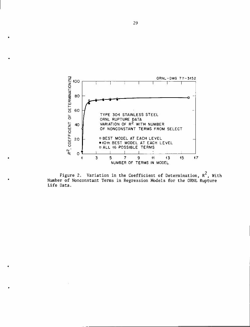
22. Variation in the Coefficient of Determination, R , With
Number of Nonconstant Terms in Regression Models for theORNL Rupture Life Data 29
3. Variation in the Standard Error of Estimate, SEE, WithNumber of Nonconstant Terms in Regression Models for theORNL Rupture Life Data 30
4. Comparison of Experimental Time to Rupture and Minimum CreepRate With Predicted Results from Models With and Without
Ultimate Tensile Strength for 20 Heats of Type 304Stainless Steel 57
5. Comparison of Experimental Time to Rupture as a Functionof Elevated-Temperature Ultimate Tensile Strength (U)With Values Predicted from Rupture Model With U forDifferent Heats of Type 304 Stainless; Tests Were at 593°C(1100°F) and 241 MPa (35 ksi) 58
6. Comparison of Experimental Time to Rupture as a Function ofElevated-Temperature Ultimate Tensile Strength (U) WithValues Predicted from Rupture Model With u for DifferentHeats of Type 304 Stainless; Tests Were at 593°C (1100°F)and 207 MPa (30 ksi) 59
7. Comparison of Experimental Time to Rupture as a Function ofElevated-Temperature Ultimate Tensile Strength (U) WithValues Predicted from Rupture Model With U for DifferentHeats of Type 304 Stainless; Tests Were at 649°C (1200°F)and 172 MPa (25 ksi) 60
8. Comparison of Experimental Time to Rupture With ValuesComputed from Models With and Without Elevated TemperatureUltimate Temperature Strength (U) for 25-mm (1-in.) Plateof Reannealed Heat 9T2796 of Type 304 Stainless Steel . . 62
9. Comparison of Experimental Time to Rupture With ValuesComputed from Models With and Without Elevated-TemperatureUltimate Tensile Strength (U) for a weak (9T2796) and aStrong Heat (8043813) 63
IX

PAGE
10. Comparison of Experimental Time to Rupture With ValuesComputed from Models With and Without Elevated-Temperature Ultimate Tensile Strength (U)' for HEDLData on Reannealed Heat 55697 64
11. Comparison of Experimental Time to Rupture With ValuesComputed from Models With and Without Elevated-TemperatureUltimate Tensile Strength (U) for Several Heats of Type304 Stainless Steel at 593°C 65
12. Comparison of Experimental Minimum Creep Rate With ValuesComputed from Models With and Without Elevated-TemperatureUltimate Tensile Strength (U) for 25-mm (1-in.) Plateof Reannealed Reference Heat of Type 304 Stainless Steel . 66
13. Comparison of Experimental Minimum Creep Rate With ValuesComputed from Models With and Without Elevated-TemperatureUltimate Tensile Strength (U) for a Weak (9T2796) and aStrong Heat (8043813) 67
14. Comparison of Experimental Minimum Creep Rate With ValuesComputed from Models With and Without Elevated-TemperatureUltimate Tensile Strength (U) for HEDL Data on ReannealedHeat 55697 68
15. Comparison of Experimental Minimum Creep Rate With ValuesComputed from Models With and Without Elevated-TemperatureUltimate Tensile Strength (U) for Several Heats ofType 304 Stainless Steel
16. Prediction of Heat-to-Heat Variations in Rupture Life forTwo Heats of Type 304 Stainless Steel
69
70
17. Prediction of Heat-to-Heat Variations in Minimum Creep Ratefor Heats 8043813 and 9T2796 of Type 304 Stainless Steel . 71
18. Plots Showing Trends in Ultimate Tensile Strength as aFunction of Test Temperature for Types 304 and 316Stainless Steel from Various Sources 75
19. Trends in Ultimate Tensile Strength as a Function of TestTemperature for ORNL Data for Type 304 Stainless Steel . . 76
20. Fits to Experimental ORNL Data for Rupture Life of Type 304Stainless Steel at 593°C (1100°F) 77
21. Fits to Experimental ORNL Data for Rupture Life of Type 304Stainless Steel at 649°C (1200°F) 78

XI
PAGE
22. Fits to Experimental ORNL Data for Minimum Creep Rateof Type 304 Stainless Steel at 593°C (1100°F) 79
23. Fits to Experimental ORNL Data for Minimum Creep ofType 304 Stainless Steel at 649°C (1200°F) 80
24. Fits to Experimental US Data for Rupture Life of Type 304Stainless Steel at 593°C (1100°F) 81
25. Fits to Experimental BSCC Data for Rupture Life of Type 304Stainless Steel at 650°C (1200°F) 82
26. Comparison of NRIM Stress-Rupture Data at 600, 650, and700°C (1112, 1202, and 1293°F) for 9 Heats of Type 304Stainless Steel in As-Received Condition With PredictedMaximum, Average, and Minimum Curves from Rupture ModelWith Elevated-Temperature Ultimate Tensile Strength (U). . 85
27. Comparison of Experimental Data With Predicted Valuesof the Plasticity Resource, es = e t ,at 593°C(1100°F). . 99
28. Comparison of Experimental Data With Predicted Valuesof the Plasticity Resource, es =e^, at 649°C (1200°F) . 100
29. Comparison of Experimental ORNL Data for the Time toTertiary Creep, tss, With Predicted Values at 593°C(1100°F) 104
30. Comparison of Experimental ORNL Data for the Average CreepRate to Tertiary Creep, e_, With Predicted Values at593°C (1100°F) 105
31. Comparison of Experimental Data With Predicted Values ofTime to the Onset of Tertiary Creep at 593°C (1100°F) and649°C (1200°F) 106
32. Comparison of Experimental Data With Predicted Values ofAverage Creep Rate to the Onset of Tertiary Creep at593°C (1100°F) and 649°C (1200°F) 107
33. Comparison of Experimental Data With Predicted Values ofCreep Strain to the Onset of Tertiary Creep at 593°C(1100°F) 109
34, Comparison of Experimental Data With Predicted Values ofCreep Strain to the Onset of Tertiary Creep at 649°C(1200°F) 110

Xll
PAGE
35. Plots of Average Creep Rate and Creep Total Elongationfor Type 304 Stainless Steel Data Collected from USand Two Foreign Countries 114
36. Predicted Trends in the Strain to the Onset of TertiaryCreep (No Offset) as a Function of Stress 118
37. Predicted Trends in the Strain to the Onset of TertiaryCreep (No Offset) as a Function of Minimum Creep Rate . . 119
38. Schematic Diagram Showing Results of Fitting Eqn. 49Directly to an Experimental Creep Curve 127
39. Schematic Illustration of the Properties of the RationalPolynomial Creep Equation 133
40. Fit of the Rational Polynomial Creep Equation to anExperimental Curve at 649°C (1200°F) 137
41. Fit of the Rational Polynomial Creep Equation to anExperimental Curve at 538°C (1000°F) 137
42. Fit of the Rational Polynomial Creep Equation to anExperimental Curve at 593°C (1100°F) 138
43. Fit of the Rational Polynomial Creep Equation to anExperimental Curve at 427°C (800°F) 139
44. Fit of the Rational Polynomial Creep Equation to anExperimental Curve at 482°C (900°F) 139
45. Relationship Between Minimum Creep Rate and Initial CreepRate for Type 304 Stainless Steel 143
46. Variation of the Rational Polynomial Creep EquationParameters With Stress at Three Temperatures for Heat9T2796, 51-mm Plate of Type 304 Stainless Steel 144
47. Comparison of Predictions With Experimental Creep Curvesfor Type 304 Stainless Steel, Including Predictions ofAverage Behavior from the Current Equation and from theBlackburn Equation 146
48. Comparison of Predictions With Experimental Creep Curvesfor Type 304 Stainless Steel, Including Predictions ofAverage Behavior from the Current Equation and from theBlackburn Equation With the Testing Conditions:Temperature = 649°C, Stress = 69 MPa 147

xm
PAGE
49. Heat-to-Heat Variations in Creep Curves of Several ReannealedHeats of Type 304 Stainless Steel 149
50. Illustrative Comparison Among Creep Data at 482°C (900°F) and427°C (800°F) and Predicted Behavior at 482°C 150
51. Comparison Between an Experimental Variable Load Creep Testfor Heat 8043813 With Predicted Behavior Using the CurrentCreep Equation and the Hypothesis of Strain Hardening ... 152
52. Comparison of Two Experimental Relaxation Curves forHeat 9T2796 at 593°C With Predicted Behavior Using theCurrent Creep Equation and the Hypothesis of StrainHardening 153
3 553. Predicted Isochronous Stress-Strain Curves at 10 - and 10 -hr
from the Creep Equation and the Rational PolynomialEquation for Average Stress-Strain Behavior 156
54. Isochronous Stress-Strain Curves at 593°C (1100°F) forHeat 9T2796, 51-mm Plate Predicted by Three Methods .... 161
55. Comparison of Stress-Temperature Operating Conditions Allowedby ASME Code Case 1592 With the Range of AvailableExperimental Creep Data for Type 304 Stainless Steel. ... 169
56. Minimum Creep Rate Data for Heat 9T2796 51-mm Plate ofType 304 Stainless Steel 175
57. Schematic Illustration of the Region of Interpolation VersusExtrapolation for Creep Data 181
58. Trends in the Tensile Reduction of Area With Temperaturefor Weak and Strong Heats of Types 304 and 316 StainlessSteel 187

INTRODUCTION
Austenitic stainless steels have gained worldwide importance as
elevated-temperature structural materials, particularly in nuclear
power generation systems. This popularity is due to several excellent
features of the behavior of these materials, including good elevated-
temperature strength, good resistance to sodium corrosion, excellent
resistance to superheated steam environments, excellent resistance to
carbon transfer, weldability, and relatively low cost [1,2]. Type 304
stainless steel exhibits excellent long-term stability with respect to
adverse microstructural changes caused by precipitation reactions [3-7].
The above properties make it possible to design components of
type 304 stainless steel for long-term service in temperature regimes
where creep and other time-dependent material properties become prime
design considerations. Power generation systems require operating
times up to and exceeding 100,000 hours, but actual experimental creep
data at such times are generally not available. Therefore, it is
necessary to predict long-term time-dependent behavior from the results
of relatively short-term tests. Most previous work in the extrapolation
of creep data has dealt with creep rupture, and many creep-rupture data
are available. However, inelastic analysis of actual operating systems
also requires a knowledge of the deformation behavior of the components
under the expected operating conditions. The prediction of such
behavior is a complex problem since, in general, components will be
subjected to variable (including cyclic) loads and temperatures and to

multiaxial states of stress. Specific methods have been developed for
making such predictions for types 304 and 316 stainless steel and for
ferritic 2 1/4 Cr-1 Mo steel [8-11], however. As listed in Ref. [11],
the components essential to such predictions are the following:
(1) a "flow rule" that relates multiaxial strain-rate components to the
corresponding multiaxial stress components; (2) a strain hardening [12]
law that describes the behavior under variable stresses; and (3) an
expression representing the behavior of the material under isothermal,
constant-load uniaxial conditions.
In the current investigation, constant-load isothermal creep
strain-time data for several heats of type 304 stainless steel tested
in air have been examined over a range of stresses and temperatures to
yield an expression for creep strain as a function of time, stress, and
temperature. The method presented here allows the creep equation to be
based largely upon readily available rupture life and minimum creep
rate data. In addition, the method provides a means of accounting for
the substantial heat-to-heat variations in properties which are
prevalent in this material [13]. The method involves development of
analytical expressions for rupture life, minimum creep rate, and time
and strain to the onset of teritary creep—all useful design properties
in themselves. Predictions made by the equation developed herein in
conjunction with the hypothesis of strain hardening are compared with
experimental relaxation and variable load data for type 304 stainless
steel.

Finally, the implications of the results in terms of material
behavior and design applications are discussed. Although elevated
temperature allowable stress values for this material are given in ASME
Code Case 1592 [14], it is shown that the current equations provide an
improved method of performing the complicated calculations involved in
the inelastic analysis of elevated-temperature components.


CHAPTER I
DESCRIPTION OF DATA USED
The data used in this investigation fall into several specific
categories. These are: (1) time to rupture (t ) data; (2) reported
minimum creep rate (e ) data; (3) various forms of creep ductility data
(ef> ©9> or e ); (4) data for the time to tertiary creep (t~ or t );
and (5) actual experimental creep curves. Figure 1 defines the various
quantities examined. All data were derived from constant-load
isothermal tests.
All material was listed in the original sources as annealed,
although it was not clear in all cases whether the material used was
mill annealed by the vendor (and tested by the laboratory in the
as-received condition), or reannealed in the laboratory before testing.
As-received material can contain residual cold work due to straightening
and forming operations occurring after the mill anneal. This cold work
can cause significant variations in yield strength, and as-received
material typically exhibits a 0.2% offset yield strength of about 35 MPa
greater than reannealed material [15,16]. However, heat treatment of
this material causes little significant microstructural change other than
the removal of such residual cold work and perhaps a small amount of
grain growth [17]. The ultimate tensile strength and creep properties
of type 304 stainless steel are virtually equivalent in the as-received
and reannealed conditions [15].

(INCLUDESLOADhNG
STRAIN)
<
I-
0.2%
ORNL-DWG 77-7214
Figure 1. Schematic Illustration of the Various Quantities Usedto Characterize the Creep Behavior of Type 304 Stainless Steel.

Rupture life (t ) data were derived from a variety of
international sources, which are described in Ref. [18]. Analysis has
shown that ultimate tensile strength is significantly reflected in the
creep and creep-rupture behavior of this material [13,19,20]. In fact,
it will be shown later in this report that many of the heat-to-heat
variations in the creep properties of this material can be described in
terms of variations in ultimate tensile strength. Therefore, it was
necessary to use only rupture data from heats of material for which
ultimate tensile strength data were also available. The data used
included data from British [21], Japanese [22] and American [13,23-29]
sources, including a large number of data recently generated at
Oak Ridge National Laboratory (ORNL)[13,25-28]. Table I summarizes
the rupture data. The various heats of material tested were too
numerous for each one to be described individually, although Table II
describes the various heats for the ORNL data.
Minimum or secondary creep rate (e ) data were available from
American sources only. These data were usually derived from the same
heats of material for which rupture life data were used. Presumably,
the values of minimum creep rate were all graphically determined from
experimental creep curves. These data, as were the rupture data, were
comprised of data from the American literature (US)[23,24,29] and from
the testing program at Oak Ridge National Laboratory (ORNL)[13,25-28].
Table III summarizes the minimum creep rate data.
In an effort to fully characterize the creep properties of type 304
stainless steel, various indices of creep ductility have also been
examined. These ductility quantities involve the strain incurred before

TABLE I
SUMMARY OF RUPTURE LIFE DATA USED
Data
Seta
Source
(Reference No.)
Number
of
Data
TemperatureRange(°C)
Stress
Range(MPa)
RuptureLife
Range(hr)
Tensile
DatabStrain
Rate
(S-1)
BSCC 21 28 600-700 62-215 23-16151 c
NRIM 22 133 600-750 47-215 30-20902-3d
1.25 x 10
US 23,24,29 146 538-816 28-345 10-65028-4e
8.3 x 10
ORNL 13,25-28 205 482-760 52-345 10-29253 6.7 x io"4
aThe data set will be referred to by this label hereafter in this
report.
bcStrain rate at which corresponding ultimate tensile strength datawere generated.
c
Strain rate not given, but assumed to be some standard rate.
Strain rates were 5 x io~5 S"1 up to 1% extension, then1.25 x IO"3.
e -5-1Strain rates specified as 8.3 x io s to the determination of
the yield strength, then 8.3 x io-4 S_l thereafter.

TABLE II
SUMMARY OF CHEMICAL ANALYSIS OF 20 HEATS OF TYPE 304 STAINLESS STEEL IN ORNL TESTING PROGRAM
Heat
SymbolChemical Element. %
C N P B 0 H Ni Mn Cr Si Mo S Nb V Ti Ta W Cu Co Pb Sn
796 0.047 0.031 0.029 0.0110 0.0006 9.58 1.22 18. S 0.47 0.10 0.012 0.008 0.037 0.003 <0.0005 0.022 0.10 0.05 0.01 0.02807 0.029 0.021 0.024 0.0005 0.010 0.0012 9.67 1.26 18.8 0.50 0.20 0.023 0.0015 0.012 0.002 <0.0005 0.020 0.11 0.03 0.01 0.01797 0.059 0.055 0.028 0.0020 0.007S 0.0007 9.78 1.49 18.3 0.60 0.30 0.110 0.0050 0.020 0.005 O.OOOS 0.050 0.30 0.07 0.002 0.0052.83 0.043 0.025 0.018 0.0003 0.0140 0.0009 9.12 1.32 18.2 0.45 0.30 0.020 0.0030 0.030 0.0010 <0.000S 0.021 0.14 0.05 0.01 0.01926 0.053 0.041 0.020 0.C084 0.0007 9.79 1.16 19.0 0.68 0.10 0.025 0.0180 0.050 0.0100 0.0010 0.030 0.070 0.05 0.010 0.02187 0.068 0.031 0.018 0.0042 0.0005 9.43 0.83 18.2 0.59 0.07 0.008 0.0020 0.060 0.003 <0.0005 0.015 0.15 0.05 0.01 0.02697 0.057 0.034 0.016 0.0150 0.0005 9.38 0.91 18.5 0.50 0.05 0.037 0.0030 0.030 0.002 <0.0005 0.011 0.10 0.05 0.01 0.02866 0.044 0.022 0.023 0.0002 0.0096 0.0010 8.98 1.51 18.5 0.47 0.2 0.007 0.0010 0.018 0.0005 0.0005 0.007 0.13 0.04 0.01 0.01544 0.063 0.019 0.023 0.0002 0.0081 0.0006 9.12 0.99 18.4 0.47 0.2 0.006 0.0050 0.025 0.017 0.0006 0.026 0.12 0.05 0.01 0.01330 0.068 0.031 0.018 0.O042 0.0005 9.43 0.83 18.2 0.59 0.07 0.008 0.0100 0.02S 0.002 <0.0005 0.0060 0.15 0.05 0.01 0.02845 0.057 0.024 0.023 0.0002 0.0092 0.0013 9.28 0.92 18.4 0.53 0.10 0.006 0.0100 0.050 0.008 <0.0005 0.007 0.11 0.07 0.01 0.01779 0.065 0.023 0.024 0.0002 0.0056 0.0009 9.46 0.94 18.1 0.47 0.20 0.005 0.003S 0.029 0.010 0.0020 0.043 0.16 0.02 0.01 0.01390 0.066 0.086 0.018 0.0020 0.0052 <0.0001 8.75 1.57 18.6 0.60 0.30 0.006 0.0160 0.020 0.001 0.0006 0.043 0.20 0.07 0.0007 0.002414 0.073 0.058 0.016 0.0190 0.0004 9.52 0.94 18.7 0.69 0.10 0.015 0.0100 0.025 0.002 <0.0005 0.027 0.10 O.OS 0.01 0.02SSI 0.043 0.027 0.022 0.0010 0.0220 0.0013 9.40 1.20 18.5 0.59 0.30 0.018 0.0140 0.050 0.025 <0.0005 0.049 0.25 0.08 0.01 0.01737 0.064 0.075 0.026 0.00005 0.0072 <0.0001 9.01 1.71 18.3 0.50 0.30 0.012 0.0140 0.031 0.001 <0.0005 0.016 0.50 0.07 <0.0003 0.0050380 0.063 0.068 0.018 0.0260 0.0009 8.30 0.97 18.4 0.55 0.07 0.010 0.0100 0.028 0.004 <0.0005 0.016 0.10 0.05 0.01 0.02086 0.050 0.043 0.025 0.0091 O.OOOS 9.46 1.23 18.4 0.53 0.20 0.016 0.0030 0.019 0.006 <0.0005 0.021 0.10 0.05 0.01 0.02813 0.062 0.033 0.044 0.0003 8.95 1.87 17.8 0.48 0.32 0.004 0.0200 0.022 0.002 <0.0005 0.02121 0.065 0.140 0.019 0.00005 0.0026 0.0011 9.19 1.92 18.1 0.30 0.14 0.010 0.0010 0.035 0.016 <0.0005 0.015 0.07 0.07 <0.0003 0.002

10
TABLE III
SUMMARY OF MINIMUM CREEP RATE DATA USED
Minimum Tensile
Creep DataNumber Temperature Stress Rate Strain
Data Source of Range Range Range RateSet (Reference No.) Data (MPa) (MPa) (% /hr) (S_1)
US 23,24,29 82 538-816 28-345 0.000015-31.3 8.3 x I0_4a
ORNL 13,25-28 226 482-760 52-345 0.000021-15.7 6.7 x 10~4
a -5 -1Strain rate specified as 8.3 x 10 S to the determination of
the yield strength, then 8.3 x 10"4 S"1 thereafter.

11
rupture and the strain incurred before the onset of tertiary creep.
Table IV lists the heats of material for which creep ductility was
examined in detail, while Table V gives the initial specimen gage
lengths and heat treatments for those heats. Table VI defines the
ranges covered by those data.
Data for the time to the onset of tertiary creep (t ) were obtained
from the same heats of material described in Tables IV and V, plus
additional data from the ORNL heat-to-heat variations program [13,26].
Values of the time to tertiary creep were determined both by the time
to first deviation from linear secondary creep (hereinafter referred to
as t?) and by a 0.2% strain offset from the linear secondary creep
portion (hereinafter referred to as t ).
Since the principal purpose of this investigation was to develop
an analytical creep strain-time expression, an important part of the
data base was a collection of experimental creep strain-time curves.
Such curves were available in quantity only for the data from the ORNL
program. Table VII defines the ranges of the available creep data from
this program. In addition, analytical fits to experimental curves from
the data of Ref. [29] were available.

TABLE IV
COMPOSITIONS AND PRODUCT FORMS OF MATERIALS INVESTIGATED IN DUCTILITY ANALYSIS
Heat Reference Product FormMn
Content, wt %a
Si Cr Ni Co Mo Cu N Nb+Ta Ti
9T2796
9T2796
55697
8043813
Type 304 Stainless Steel
28 25.4-mm plate 0.051 1.37 0.041 b 0.4 18.5 9.87 0.1 0.3 0.24 0.031 b b
13,25 50.8-nun plate 0.047 1.22 0.029 0.012 0.47 18.5 9.58 0.05 0.10 0.10 0.031 b b
29 7-mm rod 0.052 1.1 0.011 0.01 0.52 18.92 9.52 0.035 0.12 0.10 0.052 b b
27 25.2-mm plate 0.062 1.87 0.04 0.0043 0.48 17.8 8.95 0.20 0.32 0.20 0.033 b b
ASTM A 240, 30,31 Plate, rod 0.08° 2.0C 0.045c 0.03c 1.0C 17-19 8-10479
All analyses include balence iron.
Not reported.
"Maximum allowed.

13
TABLE V
HEAT TREATMENTS AND SPECIMEN GAGE LENGTHS
OF MATERIALS STUDIED IN DUCTILITY ANALYSIS
Heat, Description
9T2796, 25-mm plate
9T2796, 51-mm plate
8043813
55697
Initial
GageLength Time Temperature(mm) Treatment (hr) (°C)
Type 304 Stainless Steel
57.2a Anneal 0.5 1093
57.2 Anneal 0.5 1093
57.2a Anneal 0.5 1065
31.8 Anneal 1.0 1066
CoolingMethod
Air cool
Air cool
Air cool
Rapid aircool
Some high-stress and/or low-temperature tests were run on31.8-mm-gage-length specimens.

14
TABLE VI
SUMMARY OF DUCTILITY DATA USED
Heata
Number0
of
Data
TemperatureRange(°C)
Stress
Range(MPa)
9T2796(25.4 mm) 58 482-816 34-345
9T2796(50.8 mm) 20 538-704 55-317
55697 45 538-649 110-345
8043813 24 538-816 117-379
See Table IV, page 12, for chemical compositions.
The number of data available for different ductility criteriavaried slightly. The number given represents the total number of testsfrom which ductility data of any sort were derived.
TABLE VII
SUMMARY OF CREEP DATA USED
Heat
Number
of
Data
9T2796(25.4 mm) 67
9T2796(50.8 mm) 60
8043813 24
TemperatureRange
(°C)
Stress
Range(MPa)
Maximum
Test Time
(hr)
538-871 34-272 13,000
427-704 14-207 46,000
593-704 41-276 3200
See Table IV, page 12, for chemical compositions,

CHAPTER II
ANALYSIS OF RUPTURE LIFE AND MINIMUM
CREEP RATE DATA
The importance of creep in elevated-temperature design is well
established. Two of the most commonly reported and used material
properties as determined from creep tests are the rupture life (total
test time to rupture) and steady-state or "minimum" creep rate (slope of
the linear stage portion of a classical creep curve such as that shown
in Figure 1, page 6). The analysis of stress-rupture data has been
widely studied for many years. Some methods have attempted to rely
upon fundamental considerations of material behavior, but the current
state of understanding of the creep behavior of complex structural
alloys requires that most methods be empirical in nature. Recognizing
this fact, a method is presented here through which standard techniques
of linear regression analysis can be applied to stress-rupture and
minimum creep rate data.
Review of Previous Techniques
Various forms of graphical, numerical, parametric, and algebraic
procedures have been proposed and used with varying degrees of success.
The most widely investigated methods have involved the so-called
"time-temperature parameters," in which some parametric combination of
rupture life, t , and temperature, T, is expressed as a function of
stress, a, only:

16
P(tr, T) = f(a) . (1)
A plot of the time-temperature parameter, P, against stress then
defines the rupture behavior as a single two-dimensional "master curve,"
thus simplifying the analysis. Moreover, short-time high-temperature
data can supposedly be used to estimate long-time behavior at lower
temperatures. Time-stress, stress-temperature, and time-stress-
temperature parameters are also possible, with the total number of
proposed parameters now standing in the dozens. Several comprehensive
reviews of various parametric techniques are available [32-35].
The large number of possible analytical procedures makes the
choice of the method to use in a particular situation a formidable
task. One possible solution to this problem is the development of
flexible "generalized" parameters such as that proposed by Manson [36].
Also possible are numerical techniques based on a pointwise-defined
mesh of material properties. These techniques, such as the "minimum-
commitment method" proposed by Manson [33], or the use of finite-
difference recurrence relations [37], allow the data to numerically
determine the interrelationships among stress, temperature, and time.
Thus, the analyst is not required to specify a strict functional form
beforehand.
A standard method for selecting mathematical models to represent
phenomena in a wide range of applications involves the use of linear
regression analysis. Application of this technique to the analysis of
creep and creep-rupture data thus appears to be a logical step. In
fact, such techniques have been used for a variety of mechanical

17
properties of 2 1/4 Cr-1 Mo steel [38], including rupture data.
Rummler [39] has proposed the use of regression analysis of rupture
data, although he was concerned only with fitting data and not with
extrapolation. The technique proposed here is basically similar to
that used previously for 2 1/4 Cr-1 Mo steel. The essential features
of this technique and results for type 304 stainless steel are presented
below.
Techniques of Regression Analysis
Regression analysis is widely used in science, engineering, and
industry, and many excellent summaries of the subject are available,
such as Refs. [40] and [41]. A general description of the subject will
not be given here, although a brief introduction is necessary for an
understanding of the remainder of this chapter.
It should be remembered that the term "regression analysis" does
not imply a single rigidly defined analytical approach. In a sense,
it represents more of a general philosophy toward the analysis of data.
This philosophy basically involves first the identification of the
relevant response (dependent) and predictor (independent) variables.
Then, the predictor variables are used to form a model that best
describes the variations in the response variable within the framework
of the particular problem at hand. The exact method by which the final
model is chosen can vary widely depending upon the preference of the
individual analyst. There is no single "best" method. This chapter
illustrates a few possible approaches.

The need to summarize large masses of data by simple analytical
relationships is obvious for elevated-temperature design. For the
present purposes, it will be assumed that such relationships can be
stated in the form
y. = T 6.x.. + e. , (2)i . 3 it i
where the y. are the values of the response variable and the x.. are
the values of the predictor variables that may include combinations of
known constants, stress, temperature, or other important factors. The
3. are the coefficients multiplying the predictor variables, while e.
is an error term reflecting the random variation in y. Due to the
nature of the creep test, the rupture life (t ), or minimum creep rate
(e ), or some transformation thereof should be used as the responsev m
variable.
Equation (2) assumes that the chosen model is exactly correct and
that the 3- have some exact, though unknown, values.
In practice, this ideal situation is not found. In the case of
creep and creep-rupture data for complex alloys, the current state of
understanding of the processes involved does not allow an identification
of the "correct" physical model. Rather, the optimum empirical model is
sought, although it is not expected to be physically exact. The
coefficients 3- are then estimated by the method of least squares.
Label the estimated values of the 3- as b-. Then we have
h -1 Vi; • ™3

19
where y^^ is the predicted value of the response variable (log t or
log em) for the ith observation. The difference between predicted and
experimental values is given by
Ei =y± - h > (4)
and is denoted the ith residual. The least squares technique seeks to
minimize the sum of squares of the residuals, RSS, given by
^i-yiJ2i i
RSS =I e.2 =livi-yi)2 . (5)
Additionally, it is assumed that the residuals are normally distributed
about zero. As long as a model such as Eqn. 2 is linear in the
coefficients, RSS may be minimized by simple techniques, such as are
described elsewhere [40,41]. First, however, an appropriate model must
be identified.
Several specific decisions must be made during the process of
performing a regression analysis for a particular set of data. These
include the following steps..
1. The goals of the analysis must be established. For instance,
is fitting the data sufficient, or is extrapolation required? Are the
fits meant to describe individual heats of material, or is it necessary
to develop a general description of the behavior of a material based on
a multiheat set of data? What are the important variables whose
effects must be described? Is the requirement that of predicting time
to failure at a given stress or stress to failure at a given time?
2. The base of relevant data must be located, collected, and
screened. In the case of a multiheat data base, some sets of data may
20
still have to be treated separately. Data for different heats from
different sources with different thermomechanical processing histories
may display fundamentally different behavior. These differences may
preclude simultaneous treatment of the different data sets. On the
other hand, while a regression model may not precisely describe
heat-to-heat and heat treatment effects, a model that reflects these
effects at least to some degree may be of more general use than one that
ignores them entirely. Also, can future heats be expected to display a
distribution of behavior similar to that found in the heats for which
data are available?
3. A model must be selected. This step can be a complicated one
in general, especially in the case of creep and creep-rupture data,
which can be "messy" in terms of regression analysis. For example, data
at higher temperatures are generally collected at lower stresses. This
intercorrelation between stress and temperature can make it difficult
to isolate the effects of the individual variables. Also, data for
different heats are generally not available at the same stress-
temperature conditions.
4. Before actual use, the resulting model must be evaluated and
limitations placed on its application. Where appropriate, upper and
lower bounds on behavior may be established.
The goal of the current analysis is to develop design equations
for type 304 stainless steel. Thus, the analysis involves both
extrapolation and multiheat data sets. This situation can cause
problems, since many regression models can yield meaningless
predictions outside the range of available data. In the case of creep

21
data, metallurgical instabilities or mechanism changes can cause
problems when extrapolating (see Chapter V). Moreover, in the ideal
limit, regression analysis assumes that scatter in the data about the
predicted mean is due only to random variation. Heat-to-heat
variations in properties introduce a new nonrandom source of variation.
These problems are not thought to be insurmountable, but they indicate
the importance of extreme caution.
The data base which will be used in the current analysis was
described in the last chapter. Note that we will be using ultimate
tensile strength (U) terms in the various predictive models developed.
However, U is not a uniquely defined property even for a given heat of
material at a given temperature, but depends upon the testing
technique used to generate the tensile data. In particular, at
temperatures where creep effects are important, strain rate is an
important variable [16]. As can be seen in Table I, page 8, of the last
chapter, four major sets of stress-rupture data were available for
analysis, labeled BSCC, NRIM, US, and ORNL data. Only US and ORNL
minimum creep rate data were available. The ultimate tensile strength
data were generated at different strain rates for each of these four
data sources. Therefore, for consistency, data from each of these sets
were analyzed separately.
The remainder of this chapter is devoted to model selection and
evaluation.

22
Techniques of Model Selection
Various standard techniques for selecting optimum regression models
are available. These include the methods of forward selection, backward
elimination, stepwise regression, and several others [40]. However,
most methods have the common characteristic that they seek to isolate
a single optimum model based on statistical considerations. In the
case of creep and rupture data, such isolation is probably not
appropriate. Rather, it is preferable to isolate several potential
models and to choose one based on criteria such as physical reasonable
ness and analytical behavior when extrapolated. The most straightforward
way of determining such a list of candidate models is simply to perform
all possible regressions involving a preselected set of predictor
variables. This solution is complicated by the fact that the definition
of "best" model can become subjective. The method does, however, provide
the analyst with a variety of options.
Before choosing a list of predictor variables, one must decide upon
a choice of dependent variable. This choice has caused a surprising
amount of controversy in the case of rupture data, with some authors
favoring time as the dependent variable, and others favoring stress.
Depending upon the methods and goals of a particular analysis, perhaps
there is some question about the choice of dependent variable.
However, in performing a regression analysis, the nature of the creep
test forces time to rupture and minimum creep rate (or some
transformations thereof) to be considered as the respective dependent
variables. Here, we have chosen to use log t and log e as dependent

23
variables since the logarithmic transformation appears to yield
variables that display a normal distribution about the mean at given
levels of the predictor variables. Moreover, this normal distribution
appears to have a constant variance as a function of the predictor
variables. Both of these conditions (normal distribution and constant
variance) are implied assumptions of the linear regression techniques
used here.
The important factors in determining the value of log e or log t
appear to be applied stress (a), temperature (T) , and heat-to-heat
variability. Previous investigators [13,19,20] have shown that the
elevated-temperature ultimate tensile strength can be an effective
indicator of heat-to-heat variations in creep and rupture behavior. We
have assumed that the ultimate tensile strength (U) can be used as a
third factor in order to decrease the uncertainty caused by heat-to-heat
variations in strength, since these variations can be quite large [13].
Thus, we have
y = f(a, T, u) (6)
where y is log t or log e and the function f is formed by some linear
combination of terms which are themselves functions of a, T, and U,
plus one constant intercept form. Each term is multiplied by a
coefficient whose value is determined by a least-squares fit to the
data.
This approach contains an infinite set of possible functions.
However, we are interested here in fitting large multiple heat sets of

24
data for design purposes. Any final model chosen must not only fit the
data, but must yield reasonable and consistent extrapolations beyond
the range of the data in stress, time, and temperature. These
considerations greatly reduce the set of terms that must be considered.
Such practical considerations also greatly reduce the number of terms
that should be allowed to appear in any one model.
Even so, the number of models that must be considered is huge.
For example, in the present analyses, we considered a possible total of
sixteen terms, plus a constant term. (These terms will be enumerated
later.) Moreover, the models considered were limited to those
containing a constant term plus one to six terms in a, T, and U. The
total number of models thus under consideration was
where
N =16
6
flfi] f >
16[16]
+ + +
i> 4
16 16
1(7)
f \
m represents the total possible number of combinations of m terms
m!m
taken k at a time, k!(m-k)!
considered was 14,892!
Fortunately, methods are available for increasing computational
efficiency in the choice of subset regression models. We used the
method of LaMotte and Hocking [42,43], as implemented by a computer
program based on their SELECT subroutine.
The program first rejects many models at each level (number of
terms) as being inferior based on statistical criteria. The remaining
models at that level are ranked according to the coefficient of
determination, R2. The statistic R2 (%) is defined by
Thus the total number of models we
25
R2 =100(l -M|g.) . (8)
RSS is the residual sum of squares, given by Eqn. 5. The corrected total
sum of squares, CTSS, is given by
N
,2 «d=l
N -|2
1
CTSS= J (y.)z—±=± , (9)
2where N is the total number of data. The value of R represents the
percentage of the variation in the experimental data that can be
described by a particular model.
Input to the computer program thus consists of the experimental
data and a list of possible terms. Output consists of a ranked list
2(according to R ) of the ten best models at each level (number of terms)
These lists will in general not identify a single "best" model, but
will merely indicate a list of candidate models. The final model
selection can then be based on a combination of criteria, including
fits to data, simplicity, physical reasonableness, consistent
extrapolation, etc.
Identification of Candidate Models
The first step in the analysis for each of the six subject data
sets (BSCC, NRIM, US, and ORNL rupture data and US and ORNL minimum
rate data) was to use the SELECT subroutine to identify candidate models
for describing the stress-rupture behavior of this material according
to Eqn. 6. After several preliminary runs, a total of sixteen terms

26
were identified for input to the computer program. They are listed in
Table VIII. These terms reflect the requirement that the final
equation be simple and extrapolable. Temperature appears in the various
terms only as 1/T, rather than as more complicated functions. Since
creep is a thermally activated process, such a temperature dependence
is certainly reasonable. The ultimate tensile strength for this
material at a given strain rate can be approximately described as a
cubic polynomial in temperature [16]. The ultimate tensile strength
terms thus provide a more flexible means of describing any temperature
dependence. Note that only first order terms in stress (a) or log a
appear in Table VIII. Graphical analysis of the current data in terms
of isothermal plots of log t or log e vs log a showed no inflectionsr m °
in these plots. In fact, these curves appeared to be describable by
straight lines. If any curvature of these lines is reflected in the
data, it would be described by a model containing both a and log o
terms. Thus, the relatively simple terms given in Table VIII should
be capable of providing simple models that well describe trends in the
data, while exhibiting no inflections or analytical instabilities
when extrapolated beyond the data base.
Each of the six available data sets (four rupture and two minimum
creep rate) was individually subjected to analysis using the SELECT
procedure. In addition, the US and ORNL rupture data for type 304
stainless steel were rerun together for comparison purposes. Data from
the US, BSCC, and NRIM sources for type 316 stainless steel were also
analyzed. The results of analyses for that material are reported
elsewhere [44].

27
TABLE VIII
TERMS USED IN CHOOSING CANDIDATE MODELS THROUGH SELECT
Term Number Terma
1 1/T
2 a
3 cr/T
4 log a
5 (log a) /T
6 (log a) / (TU)
7 U
8 1/U
9 U a
LO a/U
11 1/(TU)
12 U log a
13 ± log a
14 a /(TU)
15 log (a/U)
16 U/T
aT = Temperature (K),
a = Stress (MPa),
U = Ultimate Tensile Strength at Temperature (MPa).

28
Since the SELECT program ranks candidate models according to the
2R statistic, models with more terms will have inherent advantage over
those with fewer terms. Therefore, one must limit the number of terms
in the selected models based on a compromise between statistical fit to
2data and simplicity. An example of the variation of R with number of
nonconstant terms from SELECT for the ORNL rupture data is shown in
Figure 2, where R for the best and tenth best model at each level is
plotted against the number of nonconstant terms in that model. Figure 2
2shows that R increases very rapidly in going from one to two
nonconstant terms, but increases little more in going beyond three terms.
Another useful statistic for examining these fits is the standard error
of estimate, SEE, given by
SEE - /ir^r (10)
where N is again the total number of data and v is the total number of
terms in the model. As shown in Figure 3 SEE improves (decreases) very
little in going beyond three terms. Another interesting aspect of
Figures 2 and 3 is the very small magnitude of the statistical difference
between the best and tenth best model at each level. Based on plots
such as Figures 2 and 3, models with three nonconstant terms were
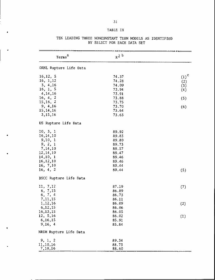
chosen for extensive study. Table IX shows the ten best three-term
models for each of the above six data sets, plus the ORNL-US combined
rupture data. The numbers in parenthesis to the right of some of the
models in Table IX indicate the number of that model as used in
subsequent analysis. Models were chosen for further study on the basis
of fits to one or more data sets and of physical reasonableness. Models
29
ORNL-DWG 77-3452
T T
TYPE 304 STAINLESS STEEL
ORNL RUPTURE DATA
VARIATION OF R2 WITH NUMBEROF NONCONSTANT TERMS FROM SELECT
©BEST MODEL AT EACH LEVEL
• 40th BEST MODEL AT EACH LEVEL
• ALL 16 POSSIBLE TERMS
I I I I I
5 7 9 11 13
NUMBER OF TERMS IN MODEL
15 17
Figure 2. Variation in the Coefficient of Determination, R , WithNumber of Nonconstant Terms in Regression Models for the ORNL RuptureLife Data.

I-<
HV)UJ
ctoororuj
Qor<Q
<
UJUJ
1.0
0.8
0.6
0.4
0.2
30
ORNL- DWG 77-3151
TTYPE 304 STAINLESS STEELORNL RUPTURE DATA
VARIATION OF SEE WITH NUMBER OFNONCONSTANT TERMS FROM SELECT
o BEST MODEL AT EACH LEVEL
• 10th BEST MODEL AT EACH LEVELo ALL 16 POSSIBLE TERMS
8—*-
5 7 9 11 13
NUMBER OF TERMS IN MODEL
15 17
N„m*Zig¥l 5' Variation in the Standard Error of Estimate, SEE, WithLife Datl " *" Re2ression Models for the ORNL Rupture
31
TABLE IX
TEN LEADING THREE NONCONSTANT TERM MODELS AS IDENTIFIED
BY SELECT FOR EACH DATA SET
Termsa R2 b
ORNL Rupture Life Data
16,12, 5 74.37 (1)C16, 1,12 74.28 (2)3, 4,16 74.09 (3)
16, 1, 5 73.94 (4)4,14,16 73.91
16, 4, 2 73.88 (5)15,16, 2 73.75
9, 4,16 73.70 (6)15,14,16 73.643,15,16 73.63
US Rupture Life Data
10, 3, 1 89.9216,14,10 89.839,10, 1 89.809, 2, 1 89.737,14,10 89.57
12,14,10 89.4714,10, 1 89.4616,12,10 89.4616, 7,10 89.4416, 4, 2 89.44 (5)
BSCC Rupture Life Data
11, 7,12 87.19 (7)6, 7,15 86.896, 7, 4 86.737.11.15 86.111.12.16 86.09 (2)6,12,15 86.06
16.13.15 86.0512, 5,16 86.02 (1)6.16.15 85.919,16, 4 85.84
NRIM Rupture Life Data
9, 1, 2 89.3411.10.16 88.737.10.16 88.60

^3
y3
4^-U
oJ>
tn
4^4
^4
^
t—•
i—>
I—•
I—1
I—1
I—'
-F
».0
0O
CM
CM
0N
)4
^O
|—I
|—1
t—•
t—•
t—•
I—'
I—*
1—'
»—*
~-J
~J
~-J
Ui
Ui
in
-si
-J
~-J
O•"-
•C
M
ON
•~4
--4
-J
--J
~-4
-J
^4
in
Ui
WO
i0
»O
^O
^
oo
oo
io
to
oM
in
sj
to
i/i
to
w<
oo
I—'
>—
'C
nC
M
c I o n o g cr
H-
3 <T>
p.
rt
C CD
r1
H-
Hi
CD
O P r+ P
^f.O
^-^W
WM
WM
t—'
I—'
h-'
I—•
h-'
lO
lO
lO
lD
tO
lO
lO
'OtO
tO
l/iln
uiw
(/iv
il/iln
l/iln
in
ln
O^^I-J^^J^^O
OW
vlW
KJW
UlW
sH
O'-J
i->
wo
\h
-'in
CM
v_
/<
—/
N>
n_
'
c H-
3 n H a> CD
TJ SO P rt
cd o p rt
P
i—i
i—•
!—•
I—1
I—'
h-'
t-1
t-1
00
00
00
00
00
00
00
00
00
00
M^lT
HO
O^O
O^-viH
ON
t-J
^J
h-1
K)
o>
—'
<—
'v
—'
H-
3 I n cd
CD SO p <T
)
O P rt
P
On
I—
SJC
O^
N]
^
t-'
H-1
I—•
h-•
cn
.p*
Cn
On
OO
OO
ON
-P^
eo
oo
ON
00
00
00
00
00
00
vl
OO
0O
00
00
on
N)
CM
CM
00
ID0
0
H CD p
50
> DO
f m x o o 3 rt
H-
3 C CD
PL
-
CM

33
aAs listed in Table VIII, page 27.
Coefficient of Determination. R2 defines the percent of variationsin the data that is described by the model.
cNumbers in parenthesis indicate the number of the given model in thefinal list of candidate models, as listed in subsequent analysis.
34
which lacked an explicit temperature term were exluded from further
study. Also excluded were models in which log t was linear in a, since
an extrapolation to zero stress would yield a finite rupture life from
such a model.
In selecting models for further study, it was decided to consider
rupture life and minimum creep rate models simultaneously, since the
candidate models for these two properties were generally similar in
form. Models for both types 304 and 316 stainless steel were treated
together. A total of fourteen three-nonconstant term models were
selected on the basis of the SELECT results for rupture life and
minimum creep rate of type 304. A fifteenth, two-term model was
chosen for further study because of previous use [13,19]. Model 16,
also a two-nonconstant term model, was chosen for study on the basis
of simplicity and fits to data. Models 17-27 were chosen for type 316
stainless steel in the same way that Models 1-14 were chosen for
type 304 stainless steel. Finally, Models 28-32 were chosen for
comparison, these models being forms of the common Larson-Miller (LM)
[45], Manson-Succop (MS)[46], and Orr-Sherby-Dorn (OSD)[47]
time-temperature parameters. Model 27, chosen through SELECT, is also
a form of the OSD parameter. The final list of thirty-two candidate
models is given in Table X.
Obviously, the list in Table X could have been made longer or
shorter. The SELECT results indicate that one is certainly not likely
to describe the current data sets much better than with the models in
this list, although there are several other models that could have been
included.

35
TABLE X
LIST OF CANDIDATE MODELS USED TO DESCRIBE RUPTURE LIFE
AND MINIMUM CREEP RATE DATA
°S a?U1. log y = aQ +-i log a +-^ + a U log a
a U
2. log y=aQ +Oj/T +-|- +a3U log a
a a
3. log y = aQ + a log a + -±- + a3U/T
4. log y=aQ +a1 U/T +a2/T +%L log a
5. log y = a- + a log a + a a + a U/T
6. log y = a„ + a log a + a Ua + a U/T
7. log y = a + c^ /(UT) + a2U + a3U log
a2 a,8. log y = aQ + a: log a + ^r log +^j
9. log y = an + a., log a + —* log a + —* a
"l10. log y = a. + — a + a_ U/T + a_ U log a
0 TU 2 3 &
11. log y = aQ + a a/T + a2 U log a + a log a
12. log y = aQ + a1 log a + a2 a/T + a3 U/T
13. log y = aQ + a2a /(TU) + a2 log (a/U) + a3/T
14. log y = aQ + aj_ log (a/U) + a^/U + a3 U/T
15. log y = aQ + o^ log a + a2 U
16. log y = a_ + aj log a + a2 U/T

36
TABLE X (continued)
17. log y = aQ + a.a + a2 log a + a3 log a/T
a218. log y = aQ + oija +-g- log a + a3 /T
19. log y = a + a..a + a2 log (a/U) + a., /T
a
20. log y = aQ + a log a + tjt- log a + a3a U
a321. log y = aQ + a1 log a + a2 a/T — log a
22. log y = aQ + o^ log a + a2 aU + a3 /T
23. log y=aQ + a1 log a+a2 /T +a3 a/(TU)
a a2
24. log y=aQ +yj- loS a + xTJ log a+a3 ° / (-TU-1
25. log y = a + a2 log a + a2 U/T + a3 U log a
26. log y = aQ + ax a /U + a2 log (a/U) + a3 /T
27. log y = aQ + a: log a + a2 a + a3 /T
28. log y = aQ + ai log a + a2 a /T + a3 /T
al29. log y = aQ +Tjr- log a + a2 a /T + a3 /T
30. log y = a„ + o^ log a + a2 /T
31. log y = a + a. log a + a2 T

32.
37
TABLE X (continued)
allog y = aQ + — log a + a2 /T
Note: y = minimum creep rate or rupture life; T = temperature (K)•o - stress (MPa). U = ultimate tensile strength at temperature (MPa);a0 - a3 = constants to be estimated by least squares.

38
Evaluation of Candidate Models
The 32 candidate models were studied as follows. First, each
model was fit by a least squares technique to each of the six basic data
sets. Then, each data set was divided into two portions: rupture data
into short-term (t <_ 2000 hr) and long-term (t > 2000 hr) data, and
minimum creep rate data into high rate (e ^_ 0.001%/hr) and low rate
(e < 0.001%/hr) data. Each of the models was next fit to the shortm
time and high rate data sets. Predictions from the models thus
obtained were then compared with the long time and low rate data to
assess the extrapolability of the various models.
Tables XI and XII present the best-fit values of the coefficients
from each of the 32 models listed in Table X for the four complete
rupture life and two complete minimum creep rate data sets respectively.
Tables XIII and XIV then show the relative successes obtained in
2fitting these models to the complete data sets in terms of R . Finally,
Tables XV and XVI show the values of the root mean square error, RMSE,
for each of the models obtained by predicting the long time and low
rate data from fits to the short time and high rate data.
RMSE =
1_RSS]2N
(11)
where N is the total number of data, and RSS the residual mean square.
N and RSS refer to the predicted (long time/low rate) data only. Since
the models were not fit directly to the long time/low rate data, the

39
TABLE XI
BEST FIT VALUES OF THE COEFFICIENTS IN THE
CANDIDATE MODELS FOR RUPTURE LIFE
Modela ao aia2 a3
ORNL Data1 0.57164E 01 -0.39149E 04 0.32601E 02 -0.73034E-02
2 0.17499E 02 -0.19782E 05 0.62477E 02 -0.21474E-01
3 0.68238E 01 -0.30856E 01 -0.30696E 01 0.11554E 02
4 0.10085E 00 0.17477E 02 0.95896E 04 -0.58833E 04
5 0.72143E 01 -0.40327E 01 -0.73095E-02 0.15262E 02
6 0.85326E 01 -0.50893E 01 -0.13614E-04 0.16734E 02
7 -0.13424E 02 0.14372E 07 0.81838E-01 -0.21507E-01
8 0.37520E 01 -0.52116E 01 0.55252E 04 -0.57080E 04
9 0.24885E 01 -0.23925E 01 0.36604E 04 -0.70614E 01
10 0.15176E 01 -0.34496E 04 0.22242E 02 -0.69045E-02
11 0.12855E 02 -0.47562E 01 0.10109E-01 -0.75057E 01
12 0.79272E 01 -0.45755E 01 -0.51099E 01 0.15888E 02
13 -0.93274E 01 -0.27193E 04 -0.29207E 01 0.11282E 05
14 -0.67699E 00 -0.43632E 01 -0.19307E 01 0.82819E 01
15 0.99715E 01 -0.64475E 01 0.21329E-01 0.0
16 0.11337E 02 -0.64000E 01 0.14755E 02 0.0
17 0.56978E 01 -0.13737E-01 -0.80948E 01 0.68691E 04
18 0.12607E 01 -0.11656E-01 -0.47263E 03 0.59133E 04
19 -0.92370E 01 0.23165E-02 -0.70631E 01 0.83044E 04
20 0.11013E 02 -0.10948E 02 0.65009E 04 -0.88710E-05
21 0.68851E 01 -0.98262E 01 -0.10745E 02 0.78241E 04
22 -0.31714E 01 -0.48628E 01 -0.26686E-05 0.14756E 05
23 -0.83205E 01 -0.23948E 00 0.12681E 05 -0.47144E 04
24 0.70545E 01 -0.10035E 04 0.60216E 06 -0.36123E 04
25 0.12188E 02 -0.69175E 01 0.12097E 02 0.17552E-02
26 -0.P0949E 01 -0.37312E 01 -0.21397E 01 0.98057E 04
27 -0.78886E 01 -0.23951E 01 -0.86600E-02 0.15324E 05
28 0.28638E 02 -0.37067E 01 -0.52129E-02 -0.19064E-01
29 -0.14630E 02 -0.33745E 04 -0.44569E 01 0.23539E 05
30 -0.22443E 01 -0.51421E 01 0.14340E 05 0.0
31 0.31167E 02 -0.54310E 01 -0.18660E-01 0.0
32 -0.14174E 02 -0.48771E 04 0.25668E 05 0.0
US Data
1 0.48168E 01 -0.28756E 04 0.37010E 02 -0.11928E-01
2 0.12139E 02 -0.12867E 05 0.56316E 02 -0.21767E-01
3 0.76023E 01 -0.34220E 01 -0.32216E 01 0.11652E 02
4 -0.45283E 01 0.13008E 02 0.16142E 05 -0.63286E 04
5 0.79928E 01 -0.43161E 01 -0.75253E-02 0.14945E 02
6 0.88909E 01 -0.51492E 01 -0.15494E-04 0.16424E 02
7 -0.11877E 02 0.13543E 07 0.76442E-01 -0.20840E-01
8 0.66829E 01 -0.73987E 01 0.63682E 04 -0.58174E 04
9 0.55808E 01 -0.48610E 01 0.46722E 04 -0.71464E 01

2 SOM
WH
HM
HH
H
HO
lO
OO
slO
Mn
^W
MH
OIO
CO
slC
Mfl*
OIW
H
o p rt
P
II
Iii
oo
oo
oo
oo
oo
oo
oo
oo
oo
oo
I—'
i—•
Ji
i—•
I—•
k-<
WW
HU
lM
(O
M
Oen
cm
en
cm
en
to
<i
Oi(/io
h-g
oID
-~J
Cm
i-1
in
-p..
--J
MlO
HH
MO
OlO
HH
HvllO
OO
*'
HH
nJW
OIO
On
JN
NH
sJO
M^
•b
O>
OM
?O
0vO
OlO
ln
WO
\H
OO
*.
Wln
OO
K)U
lvJlO
MC
I\C
OK
)(O
vlO
>tn
mtn
tn
tn
tn
tn
tn
tn
mtn
tn
tn
tn
tn
tn
tn
rn
mtn
tn
OOOOOOOOOOOOOOOOOOOOO
N)N
)M
I-'M
(O
tO
MH
MK
)H
h'H
(O
MW
HH
HH
II
II
II
II
II
II
II
II
III
OO
OO
OO
OO
OO
OO
OO
OO
OO
OO
O
*->
h->
NJ
NJ
in
on
co
i—'
CM
**
I-"
00
co
Cn
on
on
HA
Wv)
tn
tn
tn
tn
ii
OO
Oo
MM
MM
I—1
ON
ON
I—•
K)
oo
-g
oo
i-1
Cn
oO
nC
MC
Oo
en
4*
00
CM
~-J
tn
tntn
tn
i oo
oo
CM
00
ON
4^C
nen
NJK
)fcO
H0
04
NW
MN
**
On
CO
CD
>—'
O(O
~4
OO
ON
I-'4
i.O
OO
ON
Otn
tn
tn
tn
tn
tn
tn
tn
oo
oo
oo
oo
4^.•-•I-**»•(-•I—'s)h'
Ul
H*
OO(O
WO*
HOi
Cm
Cn
NJ
co
On
vj4^
Hvi
in
•—--
J.C
OC
MO
Ntn
tn
tntn
in
oo
oo
oI—
•N
JI-
"4
*4
^
II
II
III
III
OO
OO
OO
OO
OO
OO
OO
OO
OO
OO
O
CD
CD
ON
CM
•-•
I-"
O^
CO
AW
4»
*>
CO
ON
JIn
CM
4*
CM
4^
OC
nl-
1O
NW
MH
HO
)IO
tn
tn
intn
tntn
oo
oo
oo
!-•
4^
I-1
CM
NJ
K)
!-•
en
4^
4*.
CO
lOC
OM
4i
(J\
OO
)4
>U
lin
Hw
in
co
in
ni
ww
K)
Ji
tn
tn
tn
tntn
ii
oo
oo
oI—
'I—
'i—
•t-
>to
CM
Cn
-J
CO
CM
00
CM
CM
CD
Cn
4^
ON
CD
00
ON
)O
OI-
14
^tn
tn
tn
tn i
oo
oo
NJ
4=»
4^
h-"
I—'
On
ts)
K)
in
4*
ON
lH
CO
lON
)4
^42
»O
WC
MC
OW
ON
10
WH
lO
OW
HH
Htn
tntn
tntn
tni
i
OO
OO
OO
4^
N)
in
i-1
N)
NJ
oo
oo
II
II
II
II
oo
oo
oo
oo
oo
oo
oo
oo
o
I—"
00
»->
)->
CO
o•-"
(-•
t->
CO
in
1—•
4*.CD
NJ
Oo
CO
00
NJ
cn
1—•Cn
ON
otn
tn
tn
tn
tn
oo
oo
oCn
cn
in
en
J>
OO
ON
MH
MH
ON
ln
MH
HO
NH
MH
00
Hin
*W
O\0
oin
ln
4^C
0H
in
in
Cn
cn
NJi—
'CD
CO
IO
NJO
OC
DC
OO
OO
ON
CO
~-JC
MO
NO
NO
OO
tO
K)C
M4
^N
)N
J4
^N
l^O
OH
vlO
Jf'O
M-'U
lM
OlM
tn
tn
tn
tn
tn
tn
tn
tn
tn
tn
tn
tT
itn
tn
ii
ii
oo
oo
oo
oo
oo
oo
oo
I—
'Cn
NJI-'l
-'l
-'4
^l-'N
JN
J4
^N
JI-'>
-'
WW
WW
NM
MW
MN
JM
WM
HH
HH
HH
HH
HH
WH
OlO
OO
sJO
M/I^W
MH
OC
OO
OM
ON
tn
-f'W
MH
O
II
II
III
II
II
ooooooooooooooooooooooo
HW
(0
HW
--JC
MO
Ui(M
n0
0H
HW
O»
H(O
4H
00
0H
MW
UIW
WH
ON
IO
OW
NO
OO
OO
WU
HIO
NH
MM
OC
MO
N-^lK
)h
-'C
M0
4^C
no
K)--JN
JO
Ni-'C
nO
oco
en
ON
4^K
)lM
HW
*>
00
(O
OK
)^U
iN
HO
W4
vln
ln
(D
ViH
OO
ln
NjH
v)
OO
OC
O~
~IO
NO
~-4
CM
CD
CO
OO
tN
JO
N4
^K
)l-'N
)C
D^IC
DC
MK
)C
Mtn
tn
tn
tn
tn
tn
tn
tn
tisitn
tn
tn
tn
tn
tn
tn
tn
tn
tn
tn
tn
tn
tn
i
OO
OO
OO
OO
OO
OO
OO
OO
OO
OO
OO
OM
NJO
tO
N>
l-'l-'H
HH
HH
N)K
)M
I-iK
)l-'H
HI-iN
)H
1 o
1 O
i o
i o
1 O
i o
1 o
i o
1 o
1 O
1 o
i o
1 o
1 o
1 o
i o
i o
i o
1 oo
i o
1 o
i o
ON
ON
ON
4*.
-P*NJ
4*
•P*
t-1
NJ
4^.
*-•
i—14*
1—'
1—'
ON
ON
CM
NJ
J>
en
NJ
•-•^J
CM
OO
^J
K)
00
cn
oON
h-1
i—•ON
ON
00
~-JCM
CO
-J
00
en
00
^J
cn
CM
^J.CO
00
I—100
K)
NJ
CO
oCO
o1—•00
1—>
NJ
CD
CM
CD
en
o4*.CO
t-100
1—•-J
00
CM
00
Cn
00
NJ
en
ON
oJ>
^1
oCM
NJ
CM
cn
~~j
NJ
CO
ON
CM
00
4*.00
ON
i—1
NJ
4*.CM
4*
4*
ON00
o00
^1
00
NJ
ON
nj
tn
tn
tn
tn
tn
tn
tn
tn
tn
tn
tn
tn
tn
tn
mtn
mtn
tn
tn
tn
mtn
oo
oO
oo
oo
oo
oo
oo
oo
oo
oo
oo
o4*
(-•
i—•
4*.
i-'
h-•
i—•
h-"
4=>
h-•
i—•
no
NJ
NJ
i—•
i—•
*->
h->
i—•j>
h-'
i—14*
a.
CD
O
i oo
1 o
1 o
1 O
1 oo
oo
I O
1 Oo
i o
i o
i oo
o
i o
i o
i oo
o
NJ
NJ
»—•
ON
00
1—'
NO
NJ
>->
t—•
I—-
I-"00
in
N>00
(-•NJ
MCM
4*.CD
NJ
CO
oen
CM
4*.NJ
^J
en
4*
4*
^J
4*
CM
ON
ON
CO
cn
oCn
CD
CO
00
CO
--J
i—'
ON
00
CO
K)
ON
oCn
K)
J>
ON
K)
o1—'
ON
i—•
1—'
NJ
4*
00
NO
in
c?
CM
en
ON
NJ
^J
CM
CM
4*.NJ00
ON
»-•
ON
in
CO
4*
CM
ON
ON
-J
--J
1—•
in
K)
o--J
4*.CO
ON
CO
1—"
CM
CO
1—•
K)
CM
h-'00
I—'
h-"ON
NJ
CO
K)
in
CO
Otn
tn
tn
tn
in
tn
tn
mtn
tn
tn
ffltn
tn
mtn
tn
mtn
tn
tn
tn
tn
oo
oo
oo
oo
oo
oo
oo
oo
oo
oo
oo
oen
t-1cn
I-1
NJ
h-'
i—1
NJ^j
Cn4^
NJj>
i—•
CM
i—•
K)
i—1
i-1
i-1
t-'NJ
NJ
IIII
oooooooooo
NJ
N)
I—•CD
ON
en
£»•
ON
OON
^-1ON
4^
CM
NJ
OON
CD
CO
NJ
CO
4»
Ul
Avj(O
HN
NJ
ON
OO
00
ONJ
tn
tn
tn
tn
tn
tn
tn
ii
OO
Oo
oo
oin
HUi
AW
4»
4»
ooooooooooo
II
oo
1—•00
CM
i-1CO
^•J.
~J00
oi—•Cn
--J
-~JNJ
ON
t--
Cn
1—•
CO
NJ
CO
ocn
4*.
4^
CM
I—"
CO
NJ
ON
tn
tn
tn
tn
tn
tn
oo
oo
oo
en
j>
4*
in
4*.
-P»
oO
~J
I—'
I—'
*>J
I—'
ON
Oin
O*
-•vl
id
Avi
-j
t/ivi
o>
Wv|
NJ
oCn
oen
tn
tn
tn
tn
tn i
oo
oo
oH
in
N)
HH
PCM
H P CD X o o 3 rtH-
3 C CD
4^
O

p-n
H O 3 H P cr
i—•
CD X T3 P <K a> IS
)
CM
in ol --J
WW
WW
N)W
MK
)W
N)W
N)N
)H
HH
HH
NJH
O(O
OO
sJO
WJiW
WH
OIO
OO
vJO
\0
14
1C
MN
OI—
'O
(0
00
sl(M
n4
»W
NH
II
II
II
III
II
II
I
OO
OO
OO
OO
OO
OO
OO
OO
OO
OO
OO
OO
OO
OO
OO
OO
HW
WH
MH
H(O
IO
HH
WN
H4
iN
J(O
OM
/lH
OO
HH
WN
)N
slO
Oln
HV
OM
ON
CM
CO
OO
OO
ON
OI-'O
OC
OC
O-J4
^C
MO
OI-'~
JN
J(O
HH
OO
lO
OA
OO
OsH
ON
)W
4»
Wt/lW
OO
Cn
co
en
v]o
ON
ON
4iO
N>
OC
OC
00
04
iO
O
4»
ON
OO
WO
WH
ON
03
0U
10
-JO
>4
1vlH
-'O
NC
MO
ON
CO
CM
CO
ln
OC
OC
O0
NC
MC
0N
JC
MN
0N
JO
Ol-'4
^0
NC
D0
NH
OO
OO
*H
*«
30
0M
OO
<M
ON
(O
ON
OO
OI-'C
OO
Nvl<
oco
NO
Cn
vlln
vlO
N4
iC
Otn
tn
tn
tn
tn
tn
tn
tn
tn
tn
tn
triiT
itn
rritn
tn
tritn
tn
tn
tn
fn
tn
tn
tn
tn
tn
tn
tn
tn
tn
OOOOOOOOOOOOOOOOOOOOOOOOOOOOOOOO
(OMHNJWNJMHHWIOHMMHHHHHMHMOHHMHHHMHH
II
II
I
oo
oo
o
41
41
41
I—1
00
(M
On
Io
tn
slM
sio
v^l
nIO
Nvj
w*
ooo
oo
in
oo
tn
tn
tn
tn
tn
oo
oo
o4i
I—'
I—'
4^.o
ii
i
oo
oo
o
NJ
NJ
I-1
I—•
I-1
00
HNl
WON
NO
41
4*.CO
NJ
OMNHH
HN)
00
ON
CO
tn
tn
tn
tn
tn
ii
oo
oo
oin
H(n
N)
H
II
II
oo
oo
4*.
l->
On
I-1
NO
I-1
(-•00
4i
si
HM
41
NJ
41
in
Cn
NJ
CO
On
tn
tn
tn
tn
i oo
oo
i-jNJ
I-*4i
oo
oo
I-1NJ
NJ
CO
00
00
CM
Cn
oo
vi
en
oo
NJ
CD
ON
00
ON
CO
00
otn
tn
tn
tn
i oo
oo
HH
N)
ON
III
I
oo
oo
oo
4i
HH
HNJ
H4*
NJ
OCM
vl
OOn
CM
41
On
vlto
t->CO
4a.I-1NJ
in
On
CO
CM
vl
NJin
tn
tn
tn
tn
tn
tn
ii
OO
OO
Oo
HUJ
N)
MH
H
II
I
oo
oo
oo
HlO
NJ
HH
H
ONJ^ONl*
OCO
NJ
I—'CD
ON
NJ
00
Cn
ON
00
NJ00
CO
41
NO
CM
OCn
tn
tn
tn
tn
tn
tn
oo
oo
oo
in
*>
M4
iN
4>.
II
II
I
oo
oo
oo
oo
oo
Cn
41
CM
NJ
CM
COs)
si
0O
4i
CM
Cn
CM
00
On
Cn
CM
O41
00
NJ
00
Cn
II
III
oo
oo
oo
o
ON
co
si
NJ
NJ
00
NJ
on
en
sj
io
in
4^
Hto
N)
!-•On
oo
Cn
I—'CM
oo
4i
CO
On
CD
ON
vl
oo
tn
tn
tn
tn
tn
i
ON
O
Cm
cn
in
CM
cn
4*
vl
00
vl
4^-
ON
O4*
.O
-P»
on
i-1
oo
co
4*
.4
1N
J0
0•C
>IO
Osl
tn
tn
tn
tn
tn
tn
tn
tn
tn
tn
tn
tn
oo
oo
o(-
•I—
•4
^oooooooooooo
HK^OH-NjHHN)h'ln4»
1 oo
Oo
O
• oo
oo
oo
i o
1 oo
oo
o
00
h-'
NJ
h-1
I-1
1—•
(-•CM
41
vl
i—*
t—•CM
1—'
NJ
ON
41
oCO
CM
vl
I—1
ON
o41
OO
vl
oNJ
Cn
4*
J>
vl
en
NJ
CO
v]
ON
NJ
oON
ON
On
CM
vl
1—•
NJ
CO
CM
o4a.
NJ
00
O00
00
NJ
oin
4i
NJ
vl
CM
h-'
vl
CO
CM
CM
1—•
ocn
CO
CD
vl
CD
00
cn
CM
CM
CM
Cn
-P»
t-1
h-'CM
tn
tn
tn
tn
tn
tn
tn
tn
tn
tn
tn
tn
tn
tn
tn
tn
tn
oo
oo
oo
oo
oo
oo
oo
oo
oi—•
NJ
h-'
h-1
(-•
i—•
i—•
NJ
-p»j>
o4*
NO
cn
oNJ
NO
II
I
oo
oo
oo
oo
oo
oo
oo
oo
II
II
I
oooooooooo
oo
oo
oo
OO
OM
MH
HH
WH
4iH
(O
OlO
N(0
4^C
MC
Ov]io
en
i->
ON
Ovl4
^0
l-'
NJO
OC
OC
OC
OO
NI-'C
Mln
NJJiO
NC
OC
MO
N0
C0
Cn
i-'4
^C
0ln
cD
ln
0N
N0
ON
OO
vlO
NO
Oh
-'C
OC
M^N
JO
ON
OO
tn
tn
tn
tn
tn
tn
tn
tn
tn
tn
tritn
tn
ii
i
OO
OO
OO
OO
OO
OO
OC
nH
-'C
ncn
NJ4
iln
4ien
4i4
i4
i4
i
OO
HN
MIO
HH
HM
IO
MO
NM
MH
WM
O^IO
MH
WP
OW
OW
M4
^C
ni-'O
ON
CD
4^vlvio
ON
JC
OC
OW
MO
4»
H0
0U
iO
O0
N0
00
NO
0N
ON
OO
vio
co
OC
DC
nC
Mln
co
^O
Nvi
tn
tn
tn
tn
tn
tn
tn
tn
tn
tn
tn
tn
tn
tn
ii
ii
oo
oo
oo
oo
oo
oo
oo
NJ
Cn
NO
h-'
I—'
NO
Cn
I—'
MN
)4
1Is
)H
M
CO
o n o p rt
P
CM
CM
CM
NJN
JN
JN
JN
ON
JN
ON
ON
OI-'O
CO
CO
v]O
NC
n4
llM
NO
II
II
II
OOOOOOOOOO
HW
4N
HW
WO
N0
0O
NO
NW
00
CO
HOO
CO
ON
4l
00
4^
co
vj
in
co
vl
CO
NJ
ON
ON
I-1CO
K-"
CO
O4^
en
co
oo
tn
tn
tn
tn
tn
tn
tn
CO
I-1NO
vl
CO
41
ONO
4i*•
0O
0O
On
O00
CO
tn
tn
tn
tn
OOOOOOOOOOO
NO
NJ
h-"NJ
NJ
I—'
I—'
1—•t—'I—'I—•
1 O
i o
i o
i o
i o
i o
i o
1 o
1 O
1 o
1 o
ON
vl
ON
vl
vl
ON
en
41
1—"CM
vl
vl
oCO
CM
o1—•4i
ON
CO
I—"
NJ
NJ
I-1CM
oCO
41
NJ
4i
OON
CO
vl
ON
vl
CM
41
vl
CO
ON
NJ
NJ
ON
CM
oCD
4100
4^
41
O00
CM
CM
tn
tn
tn
tn
tn
tn
mtn
tn
tn
m
oo
oo
oo
oo
oo
oj>
(-•
t-*41
i—•
i—•
1—'
h-141
1—•
i—1
o
i oo
Oo
1 o
1 Oo
oO
O
CM
NJ
NO
NO
CM
CM
NJ
NJ
H-•
1—•Cn
41
CM
OCM
CM
4141
00
CO
ON
cn
ON
1—•CM
00
cn
41
CO
CM
CM
vl
O41
4i
CM
NJ
cn
ON00
41
CO
41
OO
41
NJ
41
1—•CM
en
oo
CM
o00
CO
tn
tn
tn
tn
mtn
tn
tn
tn
to
m
oo
OO
oo
oo
oo
Ocn
i—•cn
i—•CM
NJ
h-'
NO
vl
Cn
en
IIII
OOOOOOOOOOO
OO
O
5 a.
CD P
o
PN
J
CM
NJN
JH
--0
OV
14
1I-'
cn
eM
OO
ON
Cn
4ico
41
I—'ON
i—•
ON
NO
00
4i
PO
NJ
I—"CM
J>
en
00
CM
CM
NJ
oON
CD
41
41
en
vl
tn
tn
tn
tn
tn
tn
tn
tn
oo
oo
oo
oo
Cn
t-1
cn
cn
NJ
41
41
Cn
> DO
tn
o o 3 3 C CD

ON
Cn
4i
CM
NJ
t-1
II
ill
oo
oo
oo
CO
CD
vl
<o
NJ
41
en
NJ
ON
NO
vl
NO
CD
00
ON
41
I—1I—1
NO
NO
I-1CM
I-1ON
CM
CM
CO
41
I-1NJ
tn
tntn
tntn
tn
oo
oo
oo
oo
oo
oo
ON
cn
>->
in
NO
CM
41
CD
en
CM
>->
NJ
oO
NO
Co
CM
OCM
Cn00
vl
00
vl
1—'
ON
(-•ON
00
CM
tn
tn
tn
tn
tn
tn
oO
Oo
oO
i—•
i—"
NJ
i—•41
41
oo
1 oo
1 o
1 o
i—•
ON
t->
NJ
en
4i
CM
oCO
J>
vl
I—"
00
CM
NJ
oo
CO
ON
ON
CO
CO
41
I—"
00
m00
41
CM
otn
tn
to
to
to
tn
oo
oo
oo
4i
NO
in
1—'
NO
NJ
Oo
oo
oo
1—•
(-•vl
I—"NO
i—•
CO
00
>->
en
vl
CM
ON
NJ
ON
CO
oin
vl
en
(—•
NJ
vl
ON
vl
vl
vl
41
NO
l—1
tn
tn
to
mtn
to
oo
oo
oo
c co
o p rt
P
CM
CM
CM
NJN
ON
JN
JN
JN
JN
)N
JN
JN
JI-'l
-'
NJI-'O
C0
C0
vl0
NC
n4
1lM
NJI-'O
C0
00
vJO
NC
n4
iCM
NJi-
'OC
DC
OviO
Nen
4iC
MN
Oi—
•
II
II
OOOOOOOOOOO
II
ill
oooooooo
II
II
II
III
ooooooooooooo
NO
41
00
N0
CM
I—
'H
sj
4i
HH
vj
I-'I
—'I
—'
ON
HH
WM
00
I-'v
]4
lC
nN
O0
0vl0
0C
OI—
'4
iNJi-
'en
cO
Cn
CM
CM
NJC
MO
OO
NJC
OC
MN
JN
JO
i-'O
Nvii
nO
N4
iNJO
Nen
ocO
vl4
i4
1C
OO
NO
C0
41
CO
CD
CO
CO
NJC
OC
DC
MI—
'00
CM
Oln
en
cn
C0
00
00
eM
O0
NC
n4
iC0
00
Ui
(O*
HI-'N
OfH
OO
OM
ln
to
iU
DO
WO
OH
O-M
-'O
ow
ON
CM
Oln
slC
OO
viiM
4ii—
'OO
OC
MO
ON
NJO
ON
Oi—
1C
n4
ii-'O
en
i—
'ON
NJN
JO
NC
nN
Jvicn
ON
OO
oo
co
tn
tn
tn
tn
tn
tn
tn
tn
tn
tn
tn
tn
tn
tn
tn
tn
to
to
tn
tn
to
tn
tn
tn
tn
to
to
to
to
to
to
OOOOOOOOOOOOOOOOOOOOOOOOOOOOOOOO
K)l>
0H
K)M
NJW
HH
(0
NJH
NJ(0
|iJH
N)M
HI0
HN
)O
HH
WI-'P
HH
WH
II
OO
OO
OO
OO
OO
OO
OO
OO
OO
OO
OO
OO
OO
OO
OO
OO
ON
vl
vl
41
Cn
Cm
4i
ON
K)
Hv)
HC
nH
vl
CD
Cn
ON
vl
41
Cn
OO
N4
1vl
(-•
NJ
CM
vl
en
OC
DC
DN
O4
1to
to
tn
to
to
to
to
o 4i
oo
oo
oo
I—'
I—•
41
I—1
I—'
I—'
en
NJ
MON
h-•
(-•
41
t->
I—100
00
en
CM
ON
4i
NJ
ON
CO
CM
CM
00
Cn
cn
ON
CM
00
00
CM
oen
CM
4i
NJ
CO
CO
en
t-'CO
4i
NJ
Oco
CM
CM
4i
(-•00
oCO
Oco
vl
Cn
vl
CO
NJ
J>
J>
Cn
41
vl
00
CO
t-'NJ
ON
CO
CM
vl
J>
41
CO
vl
in
4i
OCn
en
NJ
vl
CO
1—'
Co
ON
NJ
00
41
ON
ON
CD
to
tn
to
to
to
tn
to
to
to
to
tn
to
tn
tn
to
to
to
to
oo
Oo
oo
oo
oo
oo
oo
oo
oO
(-•
4i
I-"
h->
NJ
NJ
NJ
1—•
1—•
1—•
i—•
1—•
J>
M(-•41
1—•
i—1
tOO
Nin
HO
NH
Wvl
en
NJ
CO
41
CO
CM
O4
10
04
1C
MC
M4
1N
JC
nO
NI-
1C
MO
NO
NO
Cm
i—1
On
ON
Cn
CM
tn
tn
to
to
to
to
tn
oo
oo
oo
ovl
MM
MH
in
4n
II
III
III
II
I1
IIII
oooooooooooooooooooooooooooooooo
CM
NJ
NO
in
ON
i—'
CM
CM
NJ
NO
Cn
I-1
h-1ON
NJ
1—"
NJ
NJ
NJ
CM
cn
1—•
41
ON
00
1—•
1—•
co
NJ
t--00
cn
vl
00
NJ
ON
4i
h-<CM
ON
NJ
OCO41
o4i
00
NO
1—•CO
CM
vl
CM
CM
NJ
ON
ON
NJ
vl
CM
ovl
oi—•
CO
NJ
vl
NJ
NO
I—1
1—•
41
41
I-"CM
CM
00
CM
NJ
vl
NO
en
NJ
en
CM
00
CO
i—1
oo
CO
1—•
NO
oCn
00
CO
CO
ON
4i
4i
CO
oCM
0N
v!
NO
ovl
ON
vl
00
(-•
oin
vl
00
CO
CO
ON
CM
vl
1—•00
00
vl00
41
NJ
00
o00
41
CO
NO
vl
ON
CM
ovl
CO
oNJ
41
ON
in
ON
CM
00
CO
NO
ON
41
vl
00
00
CM
I—141
o
to
tn
to
to
tn
to
to
tn
tn
tn
to
to
to
to
to
to
tn
to
to
to
tn
tn
to
to
to
to
to
to
to
tn
to
to
oo
oo
oo
oo
oo
oo
oo
oo
oo
oo
oo
oo
oo
oo
oo
oo
en
•-•en
(-•NJ
1—'
1—•
NJ
vl
in
en
NOen
I-1CM
NO
NJ
I—1
I—1
t-'
»->
I—1
NO
41
4>
o41
NJ
en
i-1
NJ
NJ
II
I
oooooooooo
II
II
IIII
III
oooooooooooooooooooooo
OO
OW
MM
HP
M<
»M
cn
oo
CM
Cn
oO
NO
oC
Mi-'O
NO
Nvio
NJO
OO
OO
OC
OvlO
NC
DO
OO
OO
Ovl
vlC
MO
OO
ON
4iO
vlO
Ovlt-'4
ivl
Cn
vlN
J4
iN
J4
ien
oeM
CM
CM
vlh
-'
tn
to
to
to
to
to
tn
to
tn
tn
tn
to
tn
ii
i
ooooooooooooo
Cn
i—
'Cn
cn
i-'4
i4
ien
en
4icn
in
en
I—'I
—'
(—'I
—'•
—'
OO
>—
't—
•N
HH
slO
NM
NM
slH
NH
NO
vlN
OO
en
CM
CM
OO
CM
t-'C
ncD
OO
ON
CM
O4
iC
nC
0C
nC
M0
0vi0
00
NC
M0
0i-'
4iC
M4
il-,en
0N
Cn
0N
vl0
0C
0O
O0
NvlC
MN
JO
-'^
ON
JI-'O
vlO
NC
MN
JN
Jtn
tn
tn
to
to
tn
to
to
to
to
tn
tn
to
to
•i
ii
OOOOOOOOOOOOOO
tO
(n
NN
)H
H4
lH
tO
t0
4N
|O
HP
o2
§o
c-1
(D
I—1
OP
p rt
P
pO
p pN
J
03
to
CO
H -a
> t-1
c tn
CO
o T-J
>n
OH
so
a:
to
2 mn
zo
i-itn
H2
Tl
>S
"^
DO
21-1
I-1
nto
nn
so
to
Xto
zI-H
tn
HHH
T3
CO
£S
H "3 to
r>
o > H to 5 O to
c co
41
NJ

p-a
H o 3 H p ry
h-'
CD X P O
X)
CD
in CM
cn ol vl
WW
WN
IK
)tO
WM
K)M
MN
)N
)H
HM
HH
HI-'H
I-'H
NJI-'O
CO
OO
vlO
Nln
4iC
MN
JI—
'OC
OO
OvlO
Nen
4iC
MN
O»
-'O
CO
OO
vl
Ii
ii
ii
iI
ii
ii
iI
iO
OO
OO
OO
OO
OO
OO
OO
OO
OO
OO
OO
OO
O
NJ4
14
1N
J4
1C
OI—
'vll
—'v
ll—
'I—
'I—
'I—
'to
t—'I
—'C
ON
Oh
-'C
Ol—
'I—
't-1
!—
'NO
CM
ON
CD
CM
NJC
OC
Mvll
-'v
lNJN
OC
MO
NC
DI—
'P
W--H
i4
nW
HO
OH
Cn
4iO
ln
co
CM
l-'v
iO
N4
iO
CM
CM
CM
ON
ON
vlO
NC
MC
nln
en
en
CM
Oo
cn
Oln
ON
ON
CM
ON
41
00
C0
4lN
JC
MC
OC
nN
ON
JO
OI-'l
—'4
10
0V
1V
1N
JO
NO
CM
vlvl4
1l-'v
lvlvlN
JC
MO
NN
JC
ON
Jln
OO
OO
lM
NJO
NO
Oen
CM
ON
CM
tn
to
tn
tn
to
to
to
to
to
to
to
to
tn
to
to
to
to
tn
to
to
tn
tn
to
tn
tn
to
OOOOOOOOOOOOOOOOOOOOOOOOOO
tO
tO
HK
)tO
HW
PtO
HN
)tO
MtO
HM
K)H
HK
)M
MH
N)tO
M
OOOOOOOOOOOOOOOOOOOOOOOOOO
vl
00
00
ON
00
in
CM
41
vl
to
in
OCM
41
ON
NJ
tO
O41
41
tn
to
tn
tn
oo
oo
41
I—1
I—141
On
en
NJ
4i
CM
4i
in00
CM
00
cn
oI-1CO
NJ
NJ
OO
to
to
to
to
OO
OO
ON
41
ON
I—1
CM
CO
41
ON
OO
in
in
41
4i
ONJ
oo
cn
co
oto
tn
tn
tn
oo
I-'
NJ
(-•ON
t-1
I—'vl
00
en
NJ
vl
on
oo
no
oo
en
oin
en4i
vi
nj
s]
vl
4i
ON
41
to
tn
to
to
to
II
I
oo
oo
oMN)H
HH
v]
in
NO
ON
ON
NO
00
I-1
I-1CO
00
cn
oen
I-'
Oen
NJ
ON
41
NJ
CO
NJ
on
en
to
to
to
to
tn
oo
oo
ol-i
i—'4i
I—•
I—'
I-1
h-J
I-"
NJ
NJ
Onj
en
CM
OO
OO
I-1CO
On
ONO
OO
I-1
to
to
tn
to
oo
oo
41
NO
NJ
vl
1 oO
1 Oo
oo
o
1 oo
1 oo
O
1 oO
oO
o
1 oo
oo
o
1 o
1 o
i o
1 o
CM
N>
N)
en
00
1—'
cn
CM
41
1—'
NO
h-•
I—"ON
1—'
(-•
I—1
NO
t->
ON
41
t-J4i
ON
00
CO
CO
00
NJ
1—•
NO
o00
NO
CM
CO
en
J>
CM4i
o41
00
ON
00
oen
CM
00
00
CM
vl
00
CO
NO
CM
CM
00
4i
vl
oCD00
4>
1—•
ON41
ON
Cn
cn
Cn4i
ovl
NJCM
l-J
00
NJ
ON
CM
vl
NO
vl
h-1
oo
vl
NJ
CM
41
41
h->
en
Cn
H->ON
en
ON
ON
ON
oNJ
Cn
Cn
in
00
H-•en
41
ON
CO
vl
CM
vl
en
41
NJ
en
oON
CM
CO
00
NO
CO
ON
ON
ON
vl
to
to
tn
to
to
to
to
to
to
to
mto
to
to
to
to
to
to
to
to
to
to
tn
tn
to
to
oo
Oo
oo
oo
oo
oo
Oo
oo
oo
oo
oo
oo
oO
cn
1—'
en
HNO
1—'
I—1
NO
ON
en
41
NJ
in
I—1
41
NJ
NJ
1—'
I—-
1—'
t->
1—'NO41
4i
1—'
III
II
OOOOOOOOOOOOO
II
I
oo
oo
II
I
oo
oo
oo
oo
o
OO
OW
MM
HH
WW
NM
AH
HH
OslO
OM
MO
HW
ON
Hslln
WO
ON
00
O0
CD
NJ4
10
0N
jen
N0
4l0
ON
0O
vl0
00
00
0C
MC
MC
M0
0C
n4
iC
MC
0H
ON
00
4>
t0
4iH
HW
4>
MO
OW
to
to
tn
to
to
to
to
tn
to
tn
to
to
to
II
I
OO
OO
OO
OO
OO
OO
OC
ni-'C
nen
i-'4
i4
ien
en
4iC
n4
ien
CO
NJ
en
Cn
O4
10
0h
-'N
O0
0O
Cn
o0
0H
-"O
N0
0o
CO
CO
On
CO
in
i—1
00
WH
OW
WO
OO
to
toto
toto
tnto
I
oo
oo
oo
oN
)W
IN)
HH
H4
n
OI—
'I—
'I—
'
CD p
pO
P
NJ p
CM
> DO
t-
to
X o o 3 H-
3 C CDD-
41
CM
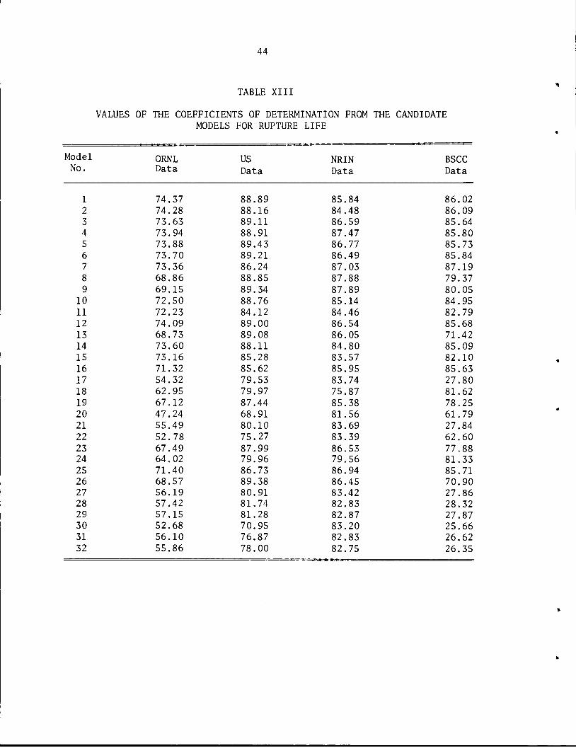
WW
lU
N)tN
)N
)N
)N
)tO
MIN
)lN
)N
)H
HH
MH
HH
HH
H'
NJI-'O
CO
OO
vlO
Nln
4iC
MN
JI—
'OC
OO
OvlO
NC
n4
iC
MN
J(-'O
CO
OO
vlO
NC
n4
iC
MN
JI—
'
cn
cn
cn
en
cn
cn
ON
viO
NO
NC
ncn
4iO
NO
NC
nvivisjO
NvivivlO
NO
Nvivivivivivivi
Cn
ON
MvlvlO
N0
0h
J4
1.v
lN
Jen
v]vlN
J4
1l--'C
MC
M0
04
1N
JN
JC
O0
OC
MC
MC
MC
MlM
4l4
1
OO
PJO
NI-'4
il-'e
n4
io
4ivi4
iN
JI-JC
OC
MC
MI-'O
NvlO
NO
Cn
i—
'CO
CM
vlo
oto
ON
NJC
M0
NO
00
Cn
NJC
0vlO
NJC
00
0C
04
iN
JC
nN
JN
J0
NO
CM
C0
CM
OC
n0
N0
NO
00
4iC
M0
0vl
v]vlvlO
00
00
0O
0C
Ovl0
0vlC
X5
ON
CI0
vlvl0
O0
O0
O0
00
OC
OO
O0
O0
OC
O0
00
00
00
00
00
00
00
NO
»-'l
-'O
C0
0N
CD
vlC
no
00
Vlt0
C0
ln
en
00
C0
C0
4i0
0C
D0
00
NC
DC
00
0C
00
00
0
OO
OC
ON
OvltO
CM
vltO
CO
Ovicn
00
4it-'O
OC
MO
NC
DN
JI-
1v]
OiH
OW
ON
NH
OO
HsJW
OO
MN
JU
OH
MO
O4
lvlC
MN
JO
Oh
-'O
OO
NJO
N4
1C
n4
1l-'C
MK
Jl-'O
NC
O
OO
OO
OO
OO
OO
OO
OO
OO
vlO
OO
OO
OO
OC
OvlO
OO
OO
OO
OO
OO
OO
OO
OO
OC
OO
OO
OO
OO
OO
OO
OO
ON
ON
OC
MN
JN
JC
MO
NO
NtO
ON
CM
CM
i—
'Cn
ln
CM
Cn
CM
4iO
NO
N4
ien
viviviO
NO
NviO
N4
ien
v]O
ON
JO
oO
o4
i4
ico
cn
cn
CM
ON
Cn
CM
OO
vito
Cn
oo
ocn
4ii—
'00
C0
O4
ivi4
iC
n4
i0
0C
nC
MO
viC
MN
JC
n4
iO
NC
MC
OC
OO
NO
Ovi4
iC
nvio
Cn
4iO
N4
ico
OO
CM
CO
vivito
oo
4i
NO
NJN
JN
JN
JN
JvlO
OO
OvlO
NN
JO
NvlO
ON
JO
OO
OC
OvlO
OO
OO
OO
OvlO
OO
OO
OO
OO
OO
OO
OO
NO
NC
nv
ico
vio
Cn
i-'v
iN
jv
ii—
'OO
i-'v
ien
Njen
i--'e
nN
04
iO
CO
viln
en
ln
ln
ON
ON
CM
ON
ON
OO
CM
OO
CD
vlC
MO
OO
NO
OvlN
JO
NO
OO
NI—
'O4
i0
Nv]t0
OC
MI—
'CO
vlO
OO
NO
OC
nN
JO
Nv
iN
JO
NO
i-,C
M0
00
4ico
en
NJO
CM
OC
ON
JO
OC
DC
nen
vito
4iC
M0
4icO
NJ
z2
OD
.•
CD
OO
P5
0rt
ZP
f
OC
PC
Ort
P oz
Pso
rt
i-h
PZ
o > H
OD
Oto
PC
Ort
np
r>J
> DO
f-
to
4i
41

WW
WN
)W
lN
)lN
)M
tO
tO
MlN
)tO
HH
HH
I-'(
-'l
-'H
HH
.—
.^
,,
k,
,_,
NJI—
'OC
OC
OvlO
Nln
4ie
MN
JI-
'OC
OO
OvlO
NC
n4
lCM
NO
I-'O
tOO
OvlO
Nen
41
CM
NO
V-'
vlv
lvlv
lvlv
lvlO
OO
Nvlv
lvlO
Nvlv
lvlC
Ovlv
lvlO
OvlO
Ovlv
lOO
OO
OO
OO
OO
OO
OO
WK
^|^
WN
JC
MO
ON
JvlO
OI-
'CM
vlv
llM
NJO
ON
CO
OO
NJC
nN
JO
OC
OC
MN
JN
JK
Jt-
'4lC
M
olo
tOC
OO
O»
inH
ln^J
>M
4N
slO
NO
>O
OO
OO
vlH
OO
IOW
HH
ON
-4ln
N)O
NO
NC
nC
MN
JO
NC
MC
MC
MC
nC
MC
MN
JN
JO
NO
N4
lvie
nO
I-'C
Oln
N0
00
00
4lN
OO
CM
I-'l
-'vl
CO
CD
CD
CO
tOC
OC
OtD
CO
tOC
OtO
tOtO
CO
CO
CD
tOC
OC
OtO
CD
tOC
OC
OC
OC
DtO
CO
CO
tO<
pC
MN
J0
4i4
i4iC
n4
ii-'
4iC
MC
MN
jen
oN
J4
i4ie
nen
cn
cn
4ie
MC
MN
Jen
lnen
cn
CM
4i
4il
-'C
Min
CM
N0
4iC
Oen
ON
CD
lMC
M4
iON
CO
Cn
ON
4i
OO
WO
NO
NtO
-4
HO
WO
NU
lO
CD
WH
4N
Ul*
Hvl
vl
in
co
i-'O
NC
Ovivi4
iO
Nto
in
oo
i—
'NO
NJln
No
en
o4
i
zS
op
.•
CD
oo
p5
0rt
ZP
f
o Pc
rt
CO
P
O > H to
> DO
f to
41
Cn

o 3 Oq rt
g CD
NO
O o o 3*
i-J
WW
WK
)N
)N
)K
)IO
MtO
MN
)N
)M
HH
HH
HN
OI-'O
CD
OO
vlO
\ln
4lC
MN
J>
-'O
tDO
OvlO
NC
n4
lC
MN
JI-'O
CO
OO
vlO
NC
n4
iCM
NJI-'
OOOOOOOOOOOOOOOOOOOOOOOOOOO
Oo
oo
o
ON
ON
viO
NO
Nvii
ncn
ON
Cn
00
vlc
ocn
ON
00
4i4
i4i4
i4iC
n4
iON
Cn
CM
4i4
i4i4
i4i4
ivlv
lto
Cn
en
NJO
I-'O
Ovlo
OO
CO
CO
Cn
4iO
OO
N4
ivll
-'N
OO
OC
MC
OO
OI-
'NJN
JO
NN
JI-
'O
NC
ON
JO
NlM
lMO
NN
OO
ON
JO
CM
4iN
Jvi4
io4
iCM
ON
OO
ln4
ioO
Oo
4i4
ien
ON
OC
M
OO
OO
OO
OO
OO
OO
I-'O
OO
OO
OO
OO
OO
OO
OO
OO
OO
4iC
no
o4
i4i4
iNJN
JO
NC
MO
NC
no
vlC
MN
JC
MN
OC
00
00
4il
-'C
nO
OO
ON
NJO
Oi-'O
CO
OO
ON
CD
NJln
vl4
iO
NJC
nO
NN
JC
MC
MN
JN
J4
1N
JC
MC
MN
0N
JN
OI-'N
JN
0l—
•l-'v
lC
MO
OO
I-'4
i4
ivl4
i4
i4
ivlN
04
ivlO
ON
OO
O4
il-'v
lNO
vlC
OO
NI-'O
Cn
vlO
N4
i4i4
iNJC
nC
MC
n
OOOOOOOOOOOOOOOOOOOOOOOOOOOOOOOO
I—1
PJl-
'l-J
NJI-
'MI-
'tO
I-'t
OI—
'NJI—
'IM
I-'l
-'l-
^eM
I—•h
Jl-
Jl-
»H
'»-'
l—'h
JI-
Jh
J^I
-'^
cn
ON
ON
Co
i-'v
lON
i-'0
\4iO
viC
MC
Mi-
-'vie
Men
NJlM
CM
vie
n4
iCM
NJN
jNJ0
4i4
iNJ
ON
i-'C
nO
oi-
'eM
ON
lno
oo
OO
N0
4ie
no
o4
iN0
4iC
nN
04
i4iN
OO
ON
i-'C
OO
NO
ON
Ji-
'Nj
hJH
JK
JJ-1
|-'|
-'O
OO
OO
I-'O
OO
I-'0
00
00
00
00
00
00
00
0C
MC
MC
MC
MC
MC
MV
lCM
Cn
vlC
»C
M0
0C
nen
CM
N0
NO
NO
vlC
MC
M4
lON
ON
NJN
JC
M4
1C
MC
MC
M^r!flt*
i^9
slH
sn
of'1
',H
o*
'a<
ivs)o
wM
tN
wo
»w
(o
oo
oo
oo
oN
JN
0C
n4
1C
M4
i4iC
0vlC
00
N0
Nvl4
i00
t-'0
0l-
-'0
0O
OC
nC
MC
0C
MC
MN
JC
0N
0l-
'Ol-
'
2 o p.
CD
OO
rt
CD
P rt
§t/
>P
f
4i
41
Ort
pC
Dr+
Cn
Prt
oz
rt
p5
0C
Drt
h-i
WP
2rt
W NO
OD
Ort
Pco
CD
rt
nin
Pn
rt
W
50
o 2 *n
i—i
H CO
-3
O
DO
<-<
> t-1
"OC
so
tn
toC
Oo •H
On
*n
H 1-1
dZ
JEC
Ntf
l
as
to
o -3 2 to
all
toC
75
CO
a:
o
-3
1-1
CO
_2
,0
so
toc
so£
-3
Cto
l-l
"Q
2H
tom
cso
so
so
oto
o>
TO
>H
OP
Tl
DO
toH >
Ol-
H>
zH
to>
o
> DO
t-
to X <
41
On

P
3*
SO P CD
O i
v o o O I—'
o\°
3*
i-S
s
WW
WM
MW
MW
MM
MM
MH
MH
HH
NJI-'O
CO
OO
vlO
Ntn
4iC
MN
JI-'O
CD
OO
vlO
NC
n4
iC
MN
JI-'O
CO
OO
vlO
NC
n4
iC
MN
JI—
'
OO
OO
OO
OO
NJO
OO
I-'O
I-'O
OI-'^O
OI-'O
I-'I-'O
OO
OO
OO
ON
OO
OO
ON
OO
vlto
mO
CO
OO
OO
l—
1vlt-<
t0
vlN
Jt-'0
0vien
0N
NJO
0N
0N
vlvltO
41
Cn
CD
ON
4iO
oen
cn
cD
00
4iO
NC
MC
ON
JO
Cn
oo
cn
cD
co
ON
CD
ON
Cn
NO
viN
Jvi4
ico
CM
i-'C
M0
NN
J0
N0
0O
00
ln
cD
NJ0
0O
ln
0N
4iN
JN
J4
i0
NC
Dvih
-'0
00
0N
04
i4
i0
Ni—
'NJN
Jln
ON
OO
OO
OI-'O
OI-'I-'O
P-'I-'O
NJN
JO
OO
OO
OO
NJN
JO
OO
OO
OO
Cn
on
CD
ON
vl
H-"
cn
vi
cm
oo
i--
vi
00
4i
41
ON
CM
00
ON
4iC
NC
MC
DO
Ovio
nvii—
'CM
CM
Cn
en
ln
vj-^i4
iN
J0
Oln
viC
MC
Ovi4
i4
1N
JO
NJN
OC
D4
1I—
'CM
vl0
04
iC
MC
OC
Dln
OO
OvlC
MO
i—
'NJN
J4
1.
OO
H0
0O
HN
O0
NW
HW
10
*0
N0
N(0
4n
00
MO
M*
OM
4n
o p-
CD
vl
OO
rt
P rt
2j!C
DP
i-1
W rt
in CM
CM
a pC
rt
rt
(OC
DP
in rt
W
< > I-1
c tn
CO
3o
to
Tl
fH
oa
:s
to
£so
oH
oto
H
Ol-
H£
z-3
HH
^a
:2
tn2
a:
CO
/O> D
O
h-t
n>
tn
CD
so
so
a:
to to
to
tn so
X < l-H
HSO
tn>
so
oH
so
otn
>o
Ho
no
>>
HP
H>
>1—
1
zT
ltn
SOo
O 2D
O-<
Tl
HH
*T3
HSO
CO
tn a >—
i
n H l-H
Z
41
vl

48
value of R for these data is meaningless—thus the use of the RMSE
statistic for these comparisons.
The next step in the analysis is the selection of an optimum model
for each of the six data sets. By virtue of the way in which the
original terms for SELECT were chosen, most of the candidate models
behave "reasonably" when extrapolated. In terms of fits to data,
several models are virtually equivalent for each data set. Thus, any
of several models could easily be chosen for each data set. There are
many ways through which an optimum model might be chosen. The simple
procedure used here for each data set was as follows. First, define
the RSS value for each model from the fit to each total data set as
RSSf and the RSS value from the extrapolation to the long time/low rate
data as RSS . Let N. be the total number of data in each total data sete f
and N be the total number of data in each long time/low rate data
set. For each data set a new. RMSE value, RMSE*, was calculated from
RSSf + RSSRMSE* = —r, n—- . (12)Nf + Ne
Also, in order to assess the overall applicability of each model to type
304 stainless steel, the four rupture life data sets were summed and
the two minimum creep rate data sets were summed to yield RMSE** as
J>SSf + £rss (13)RMSE** = .
Tables XVII and XVIII show the results of these summations, including
the rankings of the models for each individual data set.

CM
CM
CM
NJN
JN
JN
JN
JN
JN
JN
ON
ON
JI-'I
-'I
-'I
-'I
-'
NJI—
'OC
OO
OvlO
Nln
4iC
MN
JI-'O
CD
OO
vlO
NC
n4
NW
tO
HO
iO
OO
NlC
Mn
4N
WW
H
OO
OO
OO
OO
OO
OO
OO
OO
OO
OO
OO
OO
OO
OO
OO
OO
N)N
)N
)K
)N
)M
I-'H
K)H
WM
WI-'N
)|N
)H
HI-'I-'I-'H
HH
HH
HH
I-'I-'H
HC
nln
vl4
i4
ien
OO
vii-'t
oviO
Nt--'C
Oi—
'viO
NC
ncn
viC
nO
NO
NO
OO
OC
ncn
en
en
en
4i4
iN
ON
OO
NC
n4
iln
NJO
vlN
OO
NC
Mvicn
co
eM
vio
o4
itO
OviN
jco
OO
Oi-'i
—'
Mo
nlO
00
OO
OO
OO
OO
OO
OO
OO
OO
OO
OO
OO
OO
OO
OO
OO
OO
MM
4N
MN
MH
I-'M
HW
lN
)4
iH
MM
HH
h'H
HW
HH
HH
HH
HH
HH
ON
OO
OC
MN
Oin
4i4
icO
lnN
Ovie
n4
ivi(
oO
Nvie
nC
MC
MN
JC
Men
ON
ON
NJC
M4
i4iC
MN
JO
OC
00
4iO
ON
JW
CM
4iO
OC
OO
OC
no
ON
4iO
Ovlt
oen
Cn
CM
vlv
lON
OC
ON
04
i4iO
NN
O
OOOOOOOOOOOOOOOOOOOOOOOOOOOOOOOO
h-"
I—'I
—'I
—'
t-<
>->
(-•
ol-
1O
t—'>
-'>
—'I
—'h
-'l—
'O
•—
'I—
'OO
I—
'l-'l
—'N
JC
MN
J4
»O
OO
NC
DC
MI—
'41
OC
0N
0C
DI—
'ON
tOC
OvltO
00
C0
0N
ON
J0
00
00
0C
MC
0C
0O
CO
Ovl4
i0
0vlcn
l-'l-'O
OO
OO
OO
I-'O
I—
•o
co
co
oo
co
co
co
co
oco
vlvlC
MI-JC
04
1N
OO
OO
OO
N4
1
oooooooooooooooooooooooooooooooo
ON
ON
s|vlO
^O
NW
HW
tO
WO
N4
»N
)K
)O
iH
HH
WH
HP
MK
)H
MH
HH
I-'H
CO
CO
OC
OO
OtO
NJvlN
JC
OC
DC
00
4iN
J0
04
i4
i4
iN
JC
nO
NtD
vlO
ON
j4
i4
ivl4
iO
Nvl
Cn
4iN
JO
OO
Ovlo
CO
viO
NI-'C
OI—
'ln
(0
4ilO
U4
iO
>W
WH
PH
4n
OvlvH
oo
5 P.
CD
OO
pso
o Pc
rt
CO
P oz
pso
rt
1-1
P2
O0
0P
CO
rt
np
n
> r1
co
Hm
T]
oC
O
t-
oa
o T|
ztn
CD
Hso
a:
Hc
tn
h-1
tj
2H
TJ
t—\
tn
Go
oJ?
so t—
^-
>tn
rDH
t-1
o>
1—1
FROMTIME:
TJ
tn a >
so
o o H
> DO
t-
to
Tl
Hl^
rt
p-i
>n
iX
-3
CO
§<
VH
N0
°
L^J
HH
oC
O/O
oC
OT
lr:
oa:
SO>
oo
oso
<->
so
:<tn
-3
HT
JSO
to so
2tn
so
oO
>—<
SOo
n>
HT
lH
nSO
>O
oz
2C
OT
]1—
1
H CO
41
CD
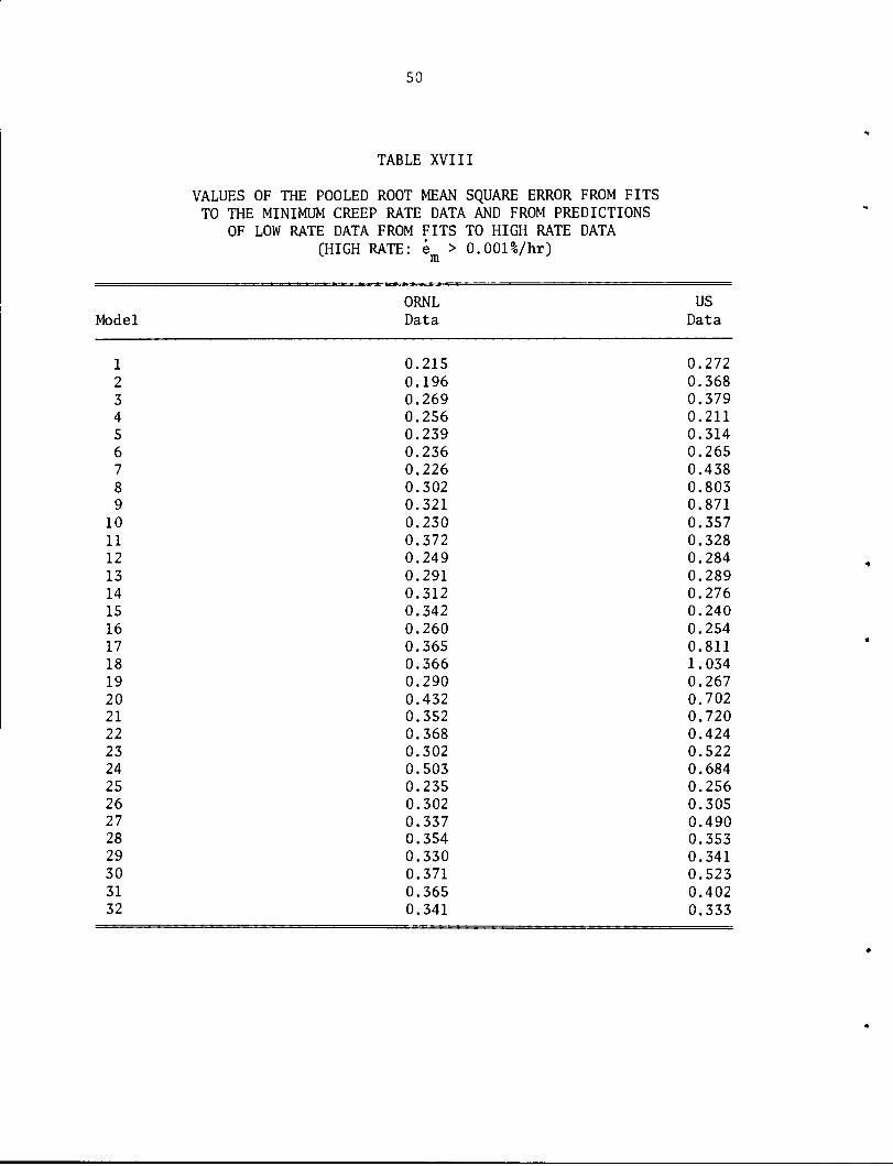
CM
CM
NJ
I—1
WW
K)M
tO
NN
)M
tO
MM
HI-'H
HH
OC
DO
OvlO
NC
n4
iC
MN
Ji—
'OC
DO
OvlO
NC
n4
nW
WH
OI0
00
s1
0N
Ui4
nW
MH
OOOOOOOOOOOOOOOOOOOOOOOOOOOOOOOO
CM
CM
CM
eM
CM
WC
MN
0ln
CM
CM
CM
41
NJC
MC
MN
JC
MC
MN
JN
0C
MN
JC
MlM
NJN
ON
JN
JN
OI-'N
04
iON
viC
Men
CM
OlM
OO
ON
Cn
eM
CO
ON
ON
ON
4i.
i—'C
04
iviC
MN
JO
N0
CM
CM
Cn
0N
C0
i-'
l-'C
nl-'0
4lv]N
Jln
eM
NJO
ON
JN
JO
ON
en
ON
ON
Oh
-'C
DN
JO
I-'N
JO
NO
NC
OO
NC
OO
NC
n
OO
OO
OO
OO
OO
OO
OO
I-'O
OO
OO
OO
OO
OO
OO
OO
OO
CM
41
lnC
MC
M4
ieM
NO
ON
ln4
lvlv
lNJO
OO
NJN
JN
ON
ON
OC
MC
M0
00
04
1N
OlM
NJC
MeM
NO
CM
ON
j4
iC
nto
oen
OO
NJN
JN
OO
ON
CM
i-'e
n4
ivlo
oo
oN
oen
vio
CM
ON
h-'i
-'v
iO
Nvi
CM
NJeM
i-'C
MO
Cn
ON
4iN
J4
iO
NJvi4
ii-'4
iO
ON
C0
4iO
Ovii-'C
MO
oen
4il-'C
OO
ON
j
o p-
CD o
oP
so
pf
O Pc
rt
CO
p
tn
•T
l
-3
> 03
f tn X <
cn
o

51
The choice of optimum models for minimum creep rate and rupture
life for the ORNL data is particularly important. Later in this report
it will be shown that the models for e and t can be useful inm r
developing a complete creep strain-time equation. Since most available
creep curves are from the ORNL data, the creep equation will be based
primarily on those data. Based on the above criteria, Model 1 is the
best rupture life model and the second best minimum creep rate model.
Interestingly, Model 2 is the best minimum creep rate model and the
second best rupture life model. Clearly, either of these models could
be used to describe both rupture life and minimum creep rate. Note
that based on the entire available data base, Model 1 yielded an RMSE**
value of 0.49 for e (the best of all models) and of 0.35 for t (them r
second best of all models). Model 2 yielded RMSE** values of 0.51 for
e and of 0.36 for t . Clearly, there is very little advantage in either
model over the other (or in fact, over several others, such as
Models 5, 6, 7). However, since Model 1 ranked ahead of Model 2 in the
overall comparisons for both properties, Model 1 was selected as optimum
for both properties for the ORNL data.
For the US data, based on RMSE* values, Model 4 ranked first for
both e and t , and thereby was considered optimum for both properties.
Note that Model 4 ranked first for t in the overall RMSE** values andr
second for e in the overall RMSE** values.m
Model 4 also ranked first for the NRIM rupture data, while Model 7
ranked first for the BSCC data. Conclusions based on the BSCC data may
be questionable due to lack of data (thus the wide variation in the

52
successes of various models for these data), but the values RMSE* and
RMSE** contain an inherent weighting factor to take the number of data
into account.
The above individual data set comparisons indicate Models 1 and 4
as perhaps the two most outstanding from the original list of 32
candidates, which themselves came from an original possible list of
over 14,000. The properties of these two models will therefore be
described here.
First, both models predict that log a vs log tr and log a vs log em
isotherms will be linear, which is not surprising for a material with
the long-term stability of type 304 stainless steel. The slopes of
these linear isotherms are given by
3log y[91og a
a
^- + a U , (14)T T 3
for Model 1 (y is e or t , the a's are coefficients as in Tables XI,m r
pages 39-41, and XII, pages 42-43). For Model 4, these slopes are given
by
oiog ySlog a
T,U
= a3 . (15)
Thus, one immediately sees a strong difference between these two models.
For Model 4, the slope is constant for all heats at all temperatures.
For Model 1, the slope is a function of both U and T. For the ORNL
data, the value of this slope can vary from -9.05 for t and 12.44 for
e for maximum strength material at 427°C to -5.08 for t and 5.80 form r

53
e for minimum strength material at 704°C. Maximum and minimum strengthm
refer to the valueUas will be defined in this chapter.
Constant stress plots of log t or log e vs. 1/T are also linearr & r & m
for both models. The slope of these iso-stress lines is given by
"8log t
3(1/T)a± log a + 0(2 U (16)
a,U
for Model 1, and by
3log t
9(1/T)= a U + a2 (17)
a,U
for Model 4. Thus, the slope is a function both of a and U for Model 1,
but is a function only of U for Model 4. Therefore Model 4 can in a
sense be viewed as a "U-modified" OSD parameter [47], since that
parameter implies such a slope to be constant.
The dependence of log t and log e upon U is also linear in both
cases, the slope of this dependence being given by
31og y3U
a„
a,T— + a_ log a (18)
for Model 1 and by
3log y3U I T T
a.
(19)
for Model 4.

54
While both Models 1 and 4 express log e or log t as functions of
a, T, and U (as they should), those models can be solved directly for
stress. For Model 1, this solution yields
(log y - a - a2-)
10«° - (.,/T «°.JJ) • (20)
(log y - a. - a. U/T - a/T)
^° -<^h — • (21)Effects of Ultimate Tensile Strength
Of the 32 candidate models listed in Table X, page 35, only
Models 17, 21, 27, 28, 29, 30, 31, and 32 lack terms reflecting ultimate
tensile strength. The first three of these were obtained from a
separate analysis of type 316 stainless steel data [44], while the last
five were chosen for study simply because they are forms of widely used
parametric models. It is not surprising that none of these models fare
very well in comparison to the entire list of models. In terms of fits
to the six total data sets, the best any of the above "non-U" models do
for R2 is Model 29, which ranks 14th best for the US minimum creep rate
data. For rupture data, the best non-U model is Model 17 which ranks
19th for the NRIM rupture data. For the extrapolated data the best
non-U model, Model 29, ranks 7th among the models for the ORNL low
minimum creep rate data, while Model 32 ranks 18th for the NRIM long
rupture life data. Table XIX illustrates the comparisons between the
best models with U terms and the best non-U models for each data set.

TABLE XIX
COMPARISON OF RESULTS OBTAINED USING MODELS WITH AND WITHOUTULTIMATE TENSILE STRENGTH TERMS
Best U MndplaFits
—
Extrancilations..
Data Set
Model
No. R (%)
Best Non-U Modela
Model
No. R (%)
Best
Model
No.
U Model a
RMSE
Best Non-
Model
No.
-U Modela
RMSE
ORNL(t ) 1 74.37 28 57.42 7 .617 28 .808
USft ) 5 89.44 28 81.74 4 .415 28 .648
NRIMft 1 8 88.28 17 83.73 4 .329 32 .395Cnin
BSCC(t ) 30 87.19 28 28.32 7 .483 32 1.16
ORNL(e )*• mJ 2 84.61 29 73.96 2 .644 29 .830
US(em) 32 95.79 29 94.56 4 .560 32 .747
From the list of candidate models given in Table X, page 35.

56
Figure 4 compares results obtained for the ORNL data using Model 1
(with U), and using Model 27, a leading non-U model.
Two conclusions can be drawn from the above comparisons. First,
the models with U terms are in general superior to those without U
terms. This superiority is particularly pronounced for the ORNL data,
which is not surprising in view of the fact that these data were
specifically generated to study heat-to-heat variations in properties
[13]. Also, it is certain that the ORNL U data were all generated at
a constant strain rate, while this fact is not as clear for the other
data—particularly the US and BSCC data. As will be discussed below,
the success obtained with models containing U terms is largely
attributable to the fact that the heat-to-heat variations in U provide
a measure of heat-to-heat variations in creep and creep-rupture
properties. A second conclusion is that our technique identified models
much better than the standard time-temperature parameters studied,
although the three standard parameters considered here form a small
subset of the total number of parameters that have been proposed.
Interestingly, both Models 1 and 4 predict a linear relationship
between log e or log t and U, consistent with the results given in
Refs. [19] and [20]. The predictions of Model 1 concerning this
relationship for the ORNL data are compared with the actual data in
Figures 5-7. These figures show considerable scatter, but it appears
that the model does accurately describe trends in the data. (Included
in these figures are data for laboratory reannealed, as-received, and
aged data, although only the reannealed data were used in the actual
modeling.)

57
o
o
trQ.
OUJ
O
OUl<ra.
'•— MODEL WITHOUT LN timatf /TENSILE STREN GTH
/ X
:©
+/x
4-
;SEE log /r = 0. 53
9 O^$/\ X
;>
+ +
:o »w
+ <
:
XX s xxa Si '"'
\
\y
(0)
0 :
-1 :
-2 :
12 3 4
log tr, EXERIMENTAL (hr)
•«,•= -3
:
MODEL WITHOUT ULTIMATET
;11 ims Lt Slh tN bl H
X y*; J<*e
+
: S!:EIog *m = 0. 56M V
X mx X
:•
. o
Aj\• o
: +** ©•»
; ++ f^m
z*1 BO
; +
; X*<
; A )
:
:
2 (c)U,U-6
-5 -4 -3 -2 -1 0
log im, EXPERIMENTAL (%/hr)
ORNL-DWG 76-10542
Q 3
:\ i
TYPE 304X
;
MODEL WITH ULTIMATE
7*
TENSILE STRENGTH
«
+
+
: SEE log tr = 0.36*t%*
4
+
\ V -
+ ya#P K+ \+
\ 9 X* '"
\ *yX
':
'Aii,
(b)
o
QUJ
? 2
12 3 4
log /r, EXPERIMENTAL (hr)
- 0 r
:
I I I I ITEMPERATURE
(°C)
o 538
- * 565
+ 593
x 649
-o 704
♦ 732
* 760
(°F)
100C
105(
11OC
120C
130(
135C
140C
X *> ,)
•)
)X
J
1X •T X +
+
)ii * •x At**
)+# H-+1
f^tM
:* +
i +
++ y* b«
:+
A fx
: SEE log em=0.44
: X
: + MODEL WITH ULTIMATE
TENSILE STRENGTHi
/ <
':/ (</)
- -1
Q
UJ
I-
y -2QUJ
cr
°l-3E
-5 -4 -3-2 1 0
log *m, EXPERIMENTAL (%/hr)
Figure 4. Comparison of Experimental Time to Rupture and MinimumCreep Rate With Predicted Results from Models With and Without UltimateTensile Strength for 20 Heats of Type 304 Stainless Steel.

10" = »
— ^vj» •
rf>co o •
—
—
o
\8u
° >o
8 M •
—
o
•
E
— ORNL DATA
T>fPE 304, 19 HE
REDICTED FROM
ATS
P ULTIMATEE
— TENSILE STRENGTH MODEL —
—
lo)—
*$ H£. 10' -
UJ
UJ
oro
2
r210
10"3
Id"4290 310 330 350 370
m3 •
o , —
o 8 ? =o ^s_
—
•
• —
~M r^^o,^ o -o
=
UJ — s6* Q —
Cd o-^9 o w3 — ^ cvo or-
Q_— •-^.p —
3 4
or 10—
o = TEST TEMPERATURE FOR BOTH —
r—
- CREEP AND TENSILE = 593°C —
Ul —
2
1— CREEP STRESS = 241 MPa
10° —
E OPEN SYMBOLS-REANNEALED m
- FILLED SYMBOLS-AS RECEIVED
(£)—
m-1
290 310 330 350 370
ULTIMATE TENSILE STRENGTH (MPa)
Figure 5. Comparison of Experimental Time to Rupture as a Function of Elevated-TemperatureUltimate Tensile Strength (U) With Values Predicted from Rupture Model with U for Different Heats ofType 304 Stainless; Tests Were at 593°C (1100°F) and 241 MPa (35 ksi).
moo

10"
— irN-210"UJ
r-
<or
o_
oro
-310
10-4
-510
PREDICTED FROM ULTIMATE TENSILESTRENGTH MODEL
ORNL DATA
TYPE 304, 17 HEATS
10'
~^210'UJ
or3r-
0_
3or
or-
J" UJ
101
icr
-110
TEST TEMPERATURE FOR BOTHCREEP AND TENSILE = 593 °C
CREEP STRESS = 207 MPa
OPEN SYMBOLS - REANNEALED
FILLED SYMBOLS-AS-RECEIVED
HALF FILLED SYMBOLS-AGED
(6)
290 310 330 350 370 290 310 330
ULTIMATE TENSILE STRENGTH (MPa)
350 370
Figure 6. Comparison of Experimental Time to Rupture as a Function of Elevated-TemperatureUltimate Tensile Strength (U) With Values Predicted from Rupture Model With u for Different Heats ofType 304 Stainless; Tests Were at 593°C (1100°F) and 207 MPa (30 ksi).
Ln
CD

10
s* N-1— 10UJ
<or
o_
UJ
or
o
r210
10"3
c410
TEST TEMPERATURE FOR BOTH —
CREEP AND TENSILE = 649°C :
CREEP STRESS =172 MPa '_
OPEN SYMBOLS - AS RECEIVED -
FILLED SYMBOLS-REANNEALED=
(a)
10
-— ?-C 10•—'
UJ
or3
r-
0_
3 1or 10
oi-
UJ
10
NH10
240 260 280 300 320 240 260 280
ULTIMATE TENSILE STRENGTH (MPa)
—
\o #
;•* • ^^-
— S%»
—
= ORNL DATA
=
..._
TYPE 304, 12 HEATS ~_
— ——
i i I
-PREDICTED FROM ULTIMATE^
— TENSILE STRENGTH MODE—
id)
300 320
Figure 7. Comparison of Experimental Time to Rupture as a Function of Elevated-TemperatureUltimate Tensile Strength (u) With Values Predicted from Rupture Model With U for Different Heats ofType 304 Stainless; Tests Were at 649°C (1200°F) and 172 MPa (25 ksi).
o
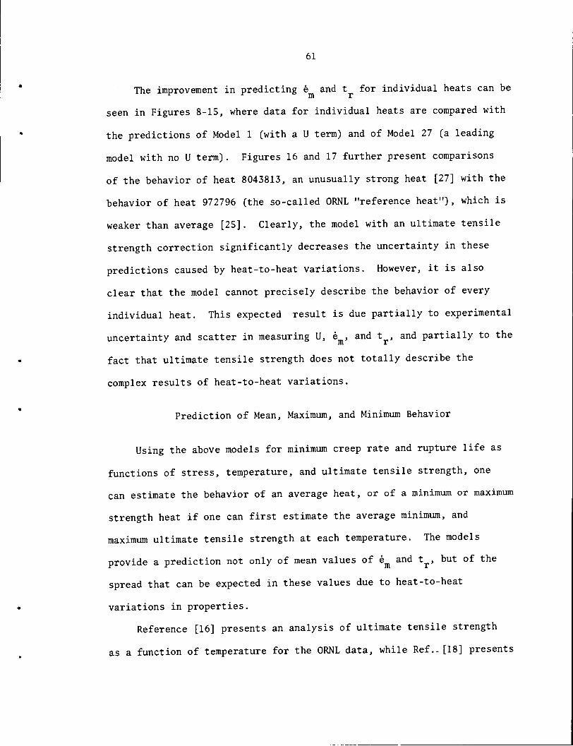
61
The improvement in predicting e and t for individual heats can be
seen in Figures 8-15, where data for individual heats are compared with
the predictions of Model 1 (with a U term) and of Model 27 (a leading
model with no U term). Figures 16 and 17 further present comparisons
of the behavior of heat 8043813, an unusually strong heat [27] with the
behavior of heat 972796 (the so-called ORNL "reference heat"), which is
weaker than average [25]. Clearly, the model with an ultimate tensile
strength correction significantly decreases the uncertainty in these
predictions caused by heat-to-heat variations. However, it is also
clear that the model cannot precisely describe the behavior of every
individual heat. This expected result is due partially to experimental
uncertainty and scatter in measuring U, e ,and tr, and partially to the
fact that ultimate tensile strength does not totally describe the
complex results of heat-to-heat variations.
Prediction of Mean, Maximum, and Minimum Behavior
Using the above models for minimum creep rate and rupture life as
functions of stress, temperature, and ultimate tensile strength, one
can estimate the behavior of an average heat, or of a minimum or maximum
strength heat if one can first estimate the average minimum, and
maximum ultimate tensile strength at each temperature. The models
provide a prediction not only of mean values of em and tr> but of the
spread that can be expected in these values due to heat-to-heat
variations in properties.
Reference [16] presents an analysis of ultimate tensile strength
as a function of temperature for the ORNL data, while Ref..[18] presents
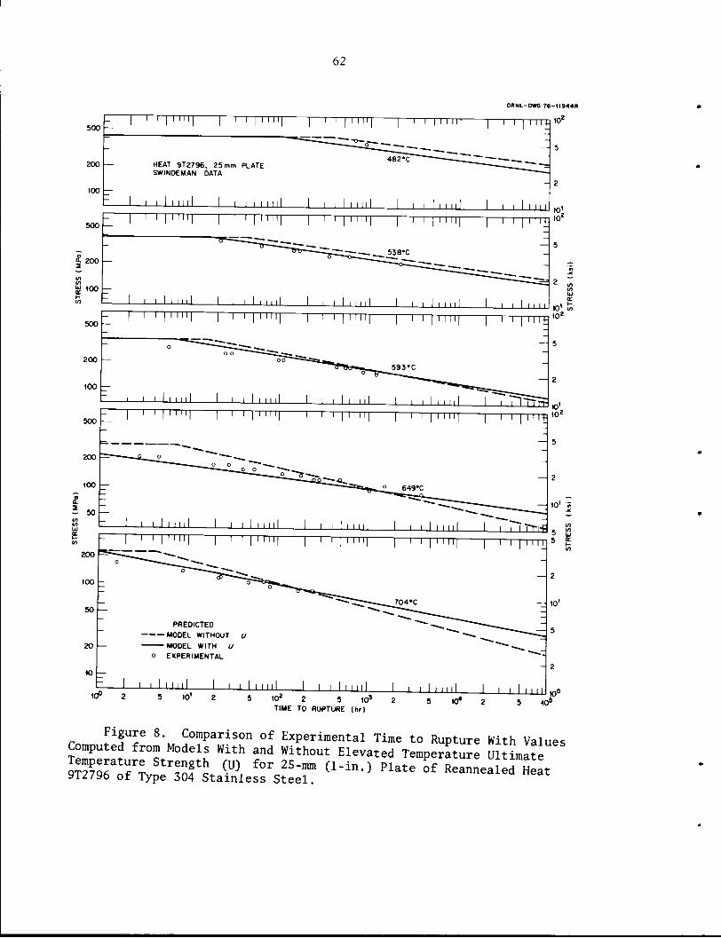
62
ORNL-DWG 76-U944R
500 —
200
100
1 ' 'I ""I I ' ' | ' '"I | ' I | IIH| 1 1 I 1IIll| 1 1 I | III.
HEAT 9T2796, 25 mm PLATESWINDEMAN DATA
482*C
500
1 I I I Mill I I I I IJJjJ 1 I I I Mill 1 'in I .,1mmZ I ' ' I ' '"I I ' ' I ' Mll I—' >IIHi| 1—l l 1Iill| 1—l-qI I ! I 11-
| 200
1—i i I i 11 il I i I I MI
Z I ' ' I ' '"I I ' ' I ' IMI I ' ' I i'li| 1—l I | Iiii| 1—i—qI I I I l
593'C
10'
10'
K)' </>102
500
200
100
500
200
100 —
— 2
I 50
200
50
-I ' I I i i il ' I i ml 1—i i I Mill 1 i i I i i nl I ""TTI-TTt~ I ' ' I ' "'I I ' ' I ' "'I I i ! 1—I I | III11 1—I I | Mil
o 649'C
10"I02
— 10' »
l ' ' 1' 'III 1 I I I Mill 1 I I I IIII! I ill I TTTTr-id gI 1 1 1—I i i i i i 1 , p—,— ~ UJ\ ' ' I "Ml I ' ' I ' "'I I I I I III11 1 1 I'M 1 I I I Mil 5 £
704«C
20 —
PREOICTED
MODEL WITHOUT U
MODEL WITH U
o EXPERIMENTAL
10 —
1 ' ' ""' 1 I I I mil 1 I I I Mill I i i I i i10° 2 5 10' 2 5 10; 5 10s 5 KJ4 2
TIME TO RUPTURE (hr)5 40s
mn. T^T 8\, ^omParison of Experimental Time to Rupture With ValuesComputed from Models With and Without Elevated Temperature UltimateSSSaTJ "'Sfc CU) f°r 25-mm (1-in') Plate °f ^annealed Seat9T2796 of Type 304 Stainless Steel.
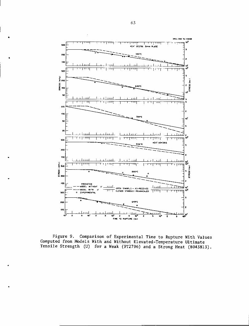
63
OftNL-DWC rt-«*4M
- 1 , , | .Ml " r- T 1 ""1 1 1 MM,.1
1 | 1 1II 1 1 1 [ 1 III
-
o
— J~~ <J»—-
~
""•'•— •»
HEAT 9T2796
593-C
51mm PLATE
•
~"
-
1 1 1 1 1 IN 1 1 Mill 1 1 1 Mlll 1 1 M 11 1 1 1
1 I I | I Ml] | I I | I1111 | 1 I | I III] 1 1 I | I lll| 1 1 I [ I III
J—I i I I I III I i i I i i ill I i i I i nil i I iinl
K>«
= I ' ' I""I I ' ' I ' "'I I ' ' I""I 1—rl | i"H 1—II | IMU <°'HEAT 8043813
J—i i I i ml 1 i i I i nil I i i I mil I i i I i ml- I i i I 11
MODEL WITHOUT U I I I I IMOOEL WITH U
o EXPERIMENTAL
I I III I I TTTTrurui Jimguui — «3-nLttlYiu *
CLOSED SYMBOLS-REANNEALED | I Il'| | I I | I I IM K>
:—I—i i 11ml I i i I i ml I i i I i ml ~~P-i-.^l~~~" ~ " • •—------ ———*• • ' •• * i i i i J ' I—-*—•- riii mi
'0° 2 S »' 2 5 IO* 2 5 10* 2 9 10* 2 5 10»TIME TO RUPTUftC <hrt
Figure 9. Comparison of Experimental Time to Rupture With ValuesComputed from Models With and Without Elevated-Temperature UltimateTensile Strength (U) for a Weak (9T2796) and a Strong Heat (8043813).

ORNL-DWG 76-H946R
500-III MINI I
'MM III 1 1 1 II II 1 1 1 1 II 1 1 1 1 II Ibt
200
<A "TJ*O 1
-^—.̂^=;538 °C
J——«—= Z=iCi5=^ =;^ ^s-. ___J
100
I I I I 1 MM III 1 1 1 || II 1 I I 1 II 1 I I 1 1 III
500 —o
0.
2
</>
[3 200ori-
100
500 —
200
100
HEAT 55697 HEDL DATA
593 °C
649 °C
PREDICTED
MODEL WITHOUT U
MODEL WITH U
o EXPERIMENTAL
15
10'
10 <
102
tn
</)
10'
5
101
10° 10 102 2 5 103TIME TO RUPTURE (hr)
10' 10:
Figure 10. Comparison of Experimental Time to Rupture With Values Computed from Models With andWithout Elevated-Temperature Ultimate Tensile Strength (U) for HEDL Data on Reannealed Heat 55697.
ONJ>
500
200 —
| 100
o: 500
200
100
500
200
4 100
OPEN SYMBOL: AS-RECEIVED
FILLED SYMBOL: REANNEALED
A BAND W DATA
65
ORNL-DWG 76-I1947R
I I I lll| 1—I I | I lll| 1—I I | I lll| 1—I I | I IthPREDICTED
MODEL WITHOUT
MOOEL WITH U
o EXPERIMENTAL
"I—I 1 | MM| 1—I I | I lll| 1—I I | I III 1—I I | Mll| 1—I I | I Ith
500F MM 11 ii| I I | I lll| 1 I I | Mll| 1 I I | IMI| 1 I I | I Ith I02 <n
UJ
HEAT 9T2796 (6 mm BAR
200
100
J i i I i ml I i i I i ml i i I iini I ii Trri-nJ
500
~ 1—I I | I lll| 1—I I | I lll| 1—I I | Mll| 1—I I | I lll| 1—I I | I Ith
200
| 100
500 —
200
100
10°
HEAT 346544
i i I i nil i i l i ml I I I Mill i i I i ml TT1TH+1—I i | I IM| 1—I I | I Ml| 1—I I | I lii| 1—I I | l lll| 1—I I 11 ith
HEAT 9T27960.20 m (B-in.l PIPE
i i I i i ill I i i I i ml I I i I i ml I I I I i ml I i T-TT-m-
10'
10* «
10"10* 10' W*
TIME TO RUPTURE (hr)
Figure 11. Comparison of Experimental Time to Rupture With ValuesComputed from Models With and Without Elevated-Temperature UltimateTensile Strength (U) for Several Heats of Type 304 Stainless Steel at593°C. The B and W data were privately supplied by Babcock and WilcoxCorp.

500
OONL-OWO 76-41948*
TTTTI 1 1 1 | I Ml[ 1 1 I | llll| 1 I I I Mll| 1 1 I | IIH| 1 1 • I I IH| I l'M'4
9T2796 25 mm PLATE
SWINDEMAN DATA
I i i I i ml I i i I i ml I i i I i i nl I i i I i ml 1—i i I I nil jjJ I i I I I n
= I I I I Mill I I I I I mil I I I I mil 1 l I I mil— I i ' I ""I I ' ' '-^-n1—i I | i ni| 1—i i | i ni] 1—I i | i 1111 1—i i | 11 •11 | I i|Mi| I i i I i mi I i ' I i i't
10'
10*
10' g10'2i«
- 2
i I i ml I i i I i ml I i i I Mill I 1 I I Mill
1—1 1 1uii| 1—1 111ni| 1—1 1 11ii'l 1—' 1 I1nil 1 1 ' M"'I I ' ' I ""i I ' ' I "
- 2
10' a
- 5
I I I I III I , 11 III
: predicted -n-rq 1 up ni| I'M ""I I'M ""I 1 » ' I '''' I I ' ' M"!MODEL WITHOUT U
MODEL WITH U
» EXPERIMENTAL
10~2 10"
MINIMUM CREEP RATE (%/hr)
(A
2 5i
5
Figure 12. Comparison of Experimental Minimum Creep Rate With Values Computed from ModelsWith and Without Elevated-Temperature Ultimate Tensile Strength (U) for 25-mm (1-in.) Plate ofReannealed Reference Heat of Type 304 Stainless Steel.
ON
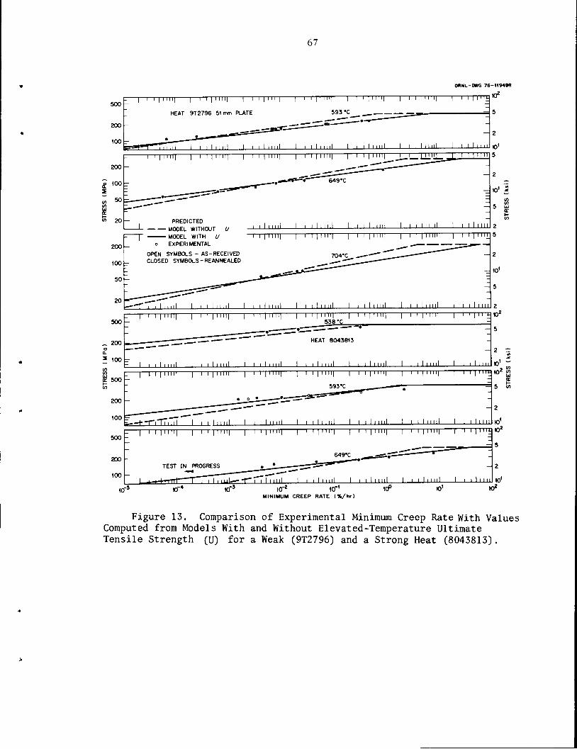
200
200
50
500
_ 200o
Q.
5 loo
E 500r-
V)
200
100
500
200
100
67
ORNL-DWG 76-11949R
111 ni|—i—i 111111|—i—i i mn|i r
HEAT 9T2796 51mm PLATE
TTT| 1 I I | Mll| T
593'C
I I | Mil 1 1 I I I ' 10*
il I i i I 11 ill I i i I 11ni I i i I 11 ni L I I i i I i ml I i I I i in
I I | llll| 1 I I | IMI] 1 I I | 11111 1 I I | llll| 1 I I I Mll| J I I I • IIM J_ ' I I
649'C
10' -*
- w
-S g
PREDICTED
-I MODEL WITHOUT U"T" MODEL WITH U
o EXPERIMENTAL
OPEN SYMBOLS - AS-RECEIVED
100L CLOSED SYMBOLS-REANNEALED
i i I mil I i i I mil I i i I i ml I I I I I llll I I I I Mil
I I | llll| 1—I I | Mll| 1—I I | Mll| 1—I I | llll| | I I I Mil
704"C
- 5
—-T I I I I nil I I I I I llll I I I I Mill I I I I Mill I I I I Mill I I I I I llll I I I I Mil
- 5
:—1 i i 1inir | i i | mii| | i i | iui| | i i | iiii| | ii- 538 °C
|llll| | 1 1 |MII| | i i | in;
- " HEAT 8043813
= I 1 1 I 1 Mil 1 1 1 1 1llll 1 1 1 1 .Mil 1 1 1 1 II III 1 II llllll 1 1 1 1 Mill 1 i ilim
:—[—tr 111ii[ | i i 111 M| | • i iiiii| | i
_ - " » —'^. — —
= 1—1 i"TTi 111 1 i i 1i ml 1 i i 1mil 1 I
M""l 1 I
593'C
1 1 Mill 1
1 | 11111
1 1 1 llll
1 1 1 |MM| | ' M '' '±
•
1 1 1 1 Mill 1 i i 1 i m
~\—I I | I1111 1—i—T | I Iii| 1—I l | MH| 1—I I | I I II | | I I JI I111 | I I | llll| | TTT
2 rr
5 a
10'MINIMUM CREEP RATE (%/hr)
Figure 13. Comparison of Experimental Minimum Creep Rate With ValuesComputed from Models With and Without Elevated-Temperature UltimateTensile Strength (U) for a Weak (9T2796) and a Strong Heat (8043813).

500
500
200
100
10"
MINI IMPPREDICTED
_ MODEL WITHOUT U
MODEL WITH U
o EXPERIMENTAL
«-410'
ttt llll INN538 °C
ORNL-DWG 76-1I950R
I I I ' ' ' 41 ?102
TTTTT1
llll Mill I I I I 'Ml 10<
HEAT 55697 HEDL DATA
llll Mill I Mill
649 °C
MINIMUM CREEP RATE (%/hr)
I I I I IIfcU <°2
I I I I 111
COCO
LC
r-
co
10<
igio2
10<
102
Figure 14. Comparison of Experimental Minimum Creep Rate With Values Computed from Models Withand Without Elevated-Temperature Ultimate Tensile Strength (u) for HEDL Data on Reannealed HeatHeat 55697.
On00
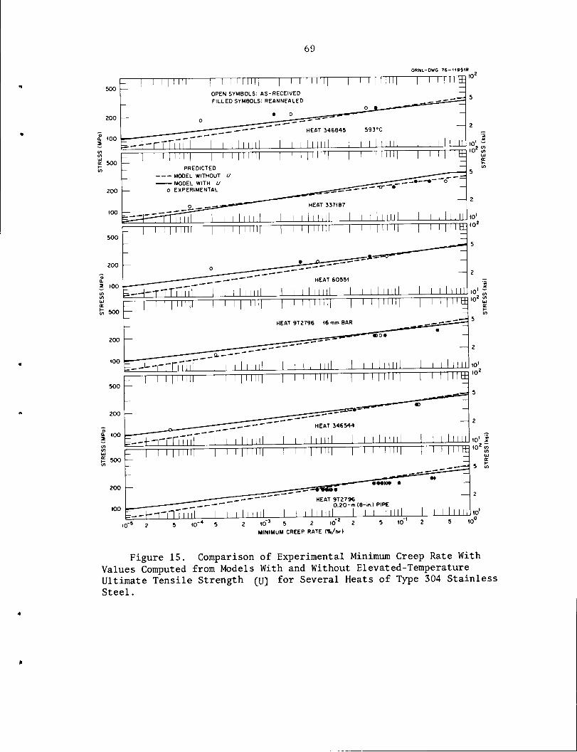
500
200
69
ORNL-DWG 76-II95IR
I i i I mil—i i i | mil I i i i nitOPEN SYMBOLS: AS-RECEIVED
FILLED SYMBOLS: REANNEALED
HEAT 346845 593°C
a. 1002 ^—4-rrrniii"" iiil mil iiil mil liil mil I i i Iun
r—MM mil 1 i i 11 mi—i i i i mil i i i i mil T TTfl
200
100
500
200
2 100
500
100
200
k 500
200
100
PREDICTED
MODEL WITHOUT U
MODEL WITH UO EXPERIMENTAL
HEAT 337187
llll llllMM mil—| i i |iiii|—| i i | mil I i i I mil I m iiitt
=•*•=•« Q—— _ — - "
— ~^ZT~- —~~~~~~ HEAT 60551rr^—r-TTnTTP"" i • i i 11 nni i i 1111111 i
I i Him 1 I I |llii| 1 I I MINI I I I MINI I m Mitt
HEAT 346544
=--T-n-iTMMT I I i Mini I i i I Illll llll Hill i I Lu|m null—i i i iiiiii—i ii r 11 •m—I I I I'Hil I l l Mitt
HEAT 9T27960.20-m(8-in.) PIPE
10'
=—h-mTnTi i iii i i i i mil, I i i 111111—I i i Inn2 10* 5 2 10 2
MINIMUM CREEP RATE (%/hr)
10 10
Figure 15. Comparison of Experimental Minimum Creep Rate WithValues Computed from Models With and Without Elevated-TemperatureUltimate Tensile Strength (u) for Several Heats of Type 304 StainlessSteel.
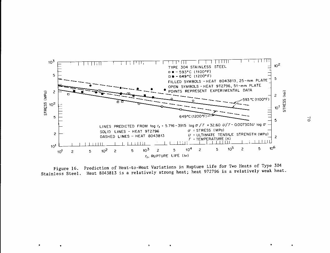
10-
oQ_
3 102LU
CO
101
101
TYPE 304 STAINLESS STEEL :
o • - 593°C (1100°F) Iurn - 649°C (1200°F)
FILLED SYMBOLS -HEAT 8043813, 25-mm PLATEOPEN SYMBOLS-HEAT 9T2796, 51-mm PLATEPOINTS REPRESENT EXPERIMENTAL DATA
593°C(1100°F)
649°C(1200°F)-
LINES PREDICTED FROM log tT =5.716-3915 logcr/T +32.60 U/T- 0.007303c/ log cr -SOLID LINES - HEAT 9T2796 cr =STRESS (MPa)DASHED LINES - HEAT 8043813 U '- ULTIMATE TENSILE STRENGTH (MPa)
T =TEMPERATURE (K)llll I llll I I I I I llll I 1 I I I UN 1 ' Ml" 1)
102
5
2 £
toCOUJ
1 orr-
CO
10
10' 103 2 5 104/r, RUPTURE LIFE (hr)
10- 10fc
Figure 16. Prediction of Heat-to-Heat Variations in Rupture Life for Two Heats of Type 304Stainless Steel. Heat 8043813 is arelatively strong heat; heat 972796 is a relatively weak heat,
o
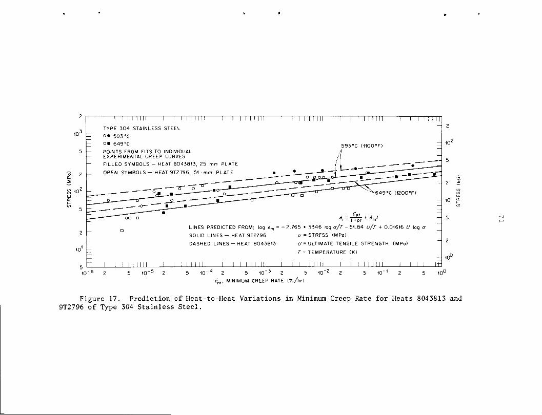
10J
P 2
10"
orp—to
10
10"
I I III 1 I I I I I III
TYPE 304 STAINLESS STEEL
°» 593 °C
•• 649°C
POINTS FROM FITS TO INDIVIDUALEXPERIMENTAL CREEP CURVES
FILLED SYMBOLS - HEAT 8043813. 25-mm PLATE
OPEN SYMBOLS — HEAT 9T2796, 51-mm PLATE
tti i i i i i i iii i—i ii 11 iii r TT
593°C (HOOT)- 10'
2 i
LINES PREDICTED FROM: log em =
SOLID LINES— HEAT 9T2796
DASHED LINES —HEAT 8043813
M I I III llll
10" 10" 10"
•2.765 + 3346 log a/T - 51.84 u/t + 0.01616 U log acr = STRESS (MPo)
U= ULTIMATE TENSILE STRENGTH (MPa)
T = TEMPERATURE (K)
10'
10"
J M _L I I III J I I llll-!
10" 10" icr
em, MINIMUM CREEP RATE (%/hr)
CO
1 or
Figure 17. Prediction of Heat-to-Heat Variations in Minimum Creep Rate for Heats 8043813 and9T2796 of Type 304 Stainless Steel.

72
such an analysis for the US, NRIM, and BSCC data. For all four data
sets, U can be described by a model of the form
U= Bo + 6XT + 62t2 + %t3 (22)
where the constants BQ, BP B2, and B3 were estimated by methods of
least squares. Table XX presents the values of these constants for
each data set, as well as the number of data and SEE value from
Eqn. 22 for each data set. The equation for the ORNL data is expressed
for temperatures in °C, while the other equations are expressed for
temperatures in °F. The so-called maximum and minimum values were
obtained by adding or subtracting twice the value of SEE from the
predicted mean. These values do not, of course, represent strict
physical maxima or minima.. Neither do they represent rigorous limits
in a statistical sense. They give a convenient measure of the width
of the scatter band for engineering purposes. However, this method
of defining limits shows reasonably good agreement with statistical
upper and lower central tolerance limits [48] for these data sets. At
a confidence level of 95%, one expects only 5% of all observations to
fall below the lower tolerance limit. Another 5% would be expected to
fall above the lower limit. For instance, Table XXI compares the
currently defined limits with these more rigorous statistical limits
for the ORNL data. The current method is preferred here for convenience
and simplicity in application. Figures 18 and 19 illustrate the
variation in U with temperature and the two methods for defining limits.
Figures 20-25 illustrate results obtained by inserting the above
mean, maximum, and minimum values of U into the optimum model for each

73
TABLE XX
BEST FIT VALUES OF COEFFICIENTS IN EQUATIONS DESCRIBING ULTIMATETENSILE STRENGTH AS A FUNCTION OF TEMPERATURE3
Number
of
Data Set Data B0 B Bi B? B* SEEb
ORNLC 135 88.90 -2.19 x 10"1 5.95 x 10"4 -5.65 x 10"7 3.40
US 272 91.93 -1.13 x io"1 1.59 x io"4 -7.84 x 10"8 3.98
NRIMd 99 95.44 -1.291 1.90 xio"4 -9.55 xio"8 2.79
BSCCd 218 89.09 -1.09 xio"1 1.51 xio"4 -7.40 xio"8 2.94
Ultimate tensile strength (U) and temperature (T) have been relatedby U = Bq + B]T + B2T2 + B3T3 strength values are given in Ksi by theseequations. To convert to MPa, the strength is multiplied by 6.895.
bStandard error of estimate for U (Ksi) by the equation in note a.
Temperatures in °C.
Temperatures in °F.

74
TABLE XXI
COMPARISON BETWEEN LOWER CENTRAL TOLERANCE LIMITS
ON ULTIMATE TENSILE STRENGTH FOR THE ORNL
DATA WITH CURRENT LIMITS
"Lower Limit" Value
of Ultimate Tensile Strength (MPa)Lower
Central Mean Value
Temperature Tolerance Minus(°C) Limit 2 x SEE*
100 441 452
200 383 397
300 366 377
400 361 369
500 341 349
600 288 296
700 165 183
aMean value given by the equation in Table XX (converted to MPa).Then twice the standard error of estimate is subtracted to give anempirical lower limit.

100
75
ORNL-DWG 76-4027
TEMPERATURE (*C)
0 200 400 600 800 0 200 400 600 800 0 200 4O0 600 8O0
800 1200 400 800 1200
TEMPERATURE CF)
400 800 1200
Figure 18. Plots Showing Trends in Ultimate Tensile Strength as aFunction of Test Temperature for Types 304 and 316 Stainless Steel fromVarious Sources. Upper- and lower-limit lines (dashed) are given by
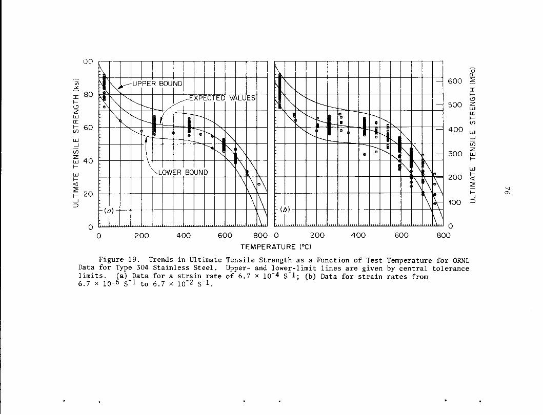
UL
TIM
AT
ET
EN
SIL
ES
TR
EN
GT
H(k
si)
ot—
'
-J
3 H-
Xrt
V)
i—"
•
OI O
V—
\
pC
O^
i
prt
rt
OP
On
Mi
•O
-J
•i
XP
O P rt
P Mi
"Tl
OH
-M
09 c
HM
CD
t-1
CO
w•
o 4^
HC
OM
rt
(D
P3
3W
oro
OO
CD
Oo
oO
o o
Ort
co3
IM
coto
pC
CO
3rt
rt
nt—
•t-
i•
Pcd
g p
o ro
O O o o CD
oo
cH
OM
>T
Jn>
"d
3
C*
(D•
MH
^J
It—
'M
l
XP 3
CD
CO
00
o*-
>C
Lrt
PI
oo
MJJ
1h
-"
-P>
.0C
D3
>o
s0
qC
CO
<T>
rt
•M
3*
-Ui-
1i
I'l
-.
|-i
PH
-w
0
/-n
3n
^rt
Pro
Oo
*-*
cC
JP
H-
3rt
3o
P(D
rt
wH
-
Ml
oO
P3
CD
n-f
c
CO
Mi
ort
0X5
oM
H-
Hp
<C
DH
-C
Dw
33
rt
hcr
Hp
XC
Drt
=1
01
CD
O*T
3o
WC
DC
Dn
3M
Mi
rt
PM
Mrt
OP
CS
>-
M CD
rt
OM
i0
0•-
•O
nC
DM
H.
O
PO
3 o CD
f
=""
"S
tr
rr1—
rrrr"tn
r
y^
V^
o^
/V
M'.
r/
/,\
I
//
c "0
.
':
*//
"O1
m
!rr
rr
CD
J
1O
N
o c.
.
:m 7
0J
12
H
;C
Do
/•I
m
Ic -z
.'
•/X "0
:o
/1
M
o
:/
s
>/
m o
i/
£;
/V C
"
;m C
O
dG
^
:"
"T
1?
Tllll
ii
jri^
^
/om
//
//
/ / /1
®/•
3<3/
3I
-y™"
B/
°/
33
p•
/
/tB
^M
9C
fm
nA
H-/
V
/^
./
yi»
o
r^
as
'e
||
|1
o o
IV)
O Oo o
o o
Ul
cn
OO
oO
UL
TIM
AT
ET
EN
SIL
ES
TR
EN
GT
H(M
Pa)
9Z

oo_
10°
£10UJtri-CO _
10'101
1 ' 1 I I I I I I 1 1 1 I I I M1 , ,TYPE 304 STAINLESS STEEL
593°C (1100°F) ORNL DATA
~~~~ MAXIMUM STRENGTH MATERIALu_ ,^~~™ «« ntm „ „™- « / AVERAGE STRENGTH—— <OP OCDO ooo rrrrrmtDTL. go ocSD o crag— — O— y nATrDi/ii
_____ a>coo^oo^c3Xrxx3--»_oc» cTcv,-/^-^ MATERIAL' • O O COOCOD
llll
MINIMUM STRENGTH MATERIAL
LINES PREDICTED FROM: log tx = 5.716- 3915 logo/7"+32.60 U/T- 0.007303 U logo-
o- = STRESS (MPa)
T= TEMPERATURE (K)
— t7= ULTIMATE TENSILE STRENGTH (MPa)
I J L I l I J_L J L llll
102 2 5 10J 2 5tt , RUPTURE LIFE (hr)
10'
"i—r I i i i
llll
10'
2 i
coco
IO1 (_jCO
10
Figure 20. Fits to Experimental ORNL Data for Rupture Life of Type 304 Stainless Steel at593°C (1100°F). Lines are predictions from Model 1 for estimated average, minimum, and maximumultimate tensile strength levels.

10~
o 2CL
2~—
CO 10^COUJ
cr
CO
10'IO1
i—r i i i i i ii i
TYPE 304 STAINLESS STEEL649°C (1200°F) ORNL DATA
"i r
^MAXIMUM STRENGTH MATERIAL
i i i i "i—r i i i i
- \0C
AVERAGE STRENGTH MATERIAL CO
? JC
—
COCO
IO1UlCC1—CO
MINIMUM STRENGTH MATERIAL
LINES PREDICTED FROM: log tr = 5.716 -3915 logo-/ 7"+32.60 U/T-0.007303 U logo-
o-= STRESS (MPa)
T= TEMPERATURE (K)
67= ULTIMATE TENSILE STRENGTH (MPa) , ,1 1—i—i i i i i I i i t i i i i i i I i i I i i i i
10< 5 IO-3 2
/r, RUPTURE LIFE (hr)
10^
J L I I I I I
2
105
Figure 21. Fits to Experimental ORNL Data for Rupture Life of Type 304 Stainless Steel at649 C (1200°F). Lines are predictions from Model 1 for estimated average, minimum, and maximumultimate tensile strength levels.
00

icr
o 20-
8 10LUor\-co
TYPE 304 STAINLESS STEEL
593 °C (1100 °F) -ORNL DATAAVERAGE STRENGTH MATERIAL
MAXIMUM STRENGTH MATERIAL
••roan*.
MINIMUM STRENGTH MATERIAL
LINES PREDICTED FROM:log em =-2.765 +3346 Iogo77"-51.84 U/T+ 0.01616 U log a
a = STRESS (MPa)
T = TEMPERATURE (K)
U = ULTIMATE TENSILE STRENGTH (MPa)
1 I Mill10
,-510' 10,-310' 10" 10"
<?m, MINIMUM CREEP RATE (%/hr)
— 10'
— 2 "coCO
10' lo
10u
Figure 22. Fits to Experimental ORNL Data for Minimum Creep Rate of Type 304 Stainless Steelat 593°C (1100°F). Lines are predictions from Model 1 for estimated average, minimum, and maximumultimate tensile strength levels.
CD

10
o
a.
10-5
10
LINES PREDICTED FROM: log em =- 2.765 + 3346 log ct/T - 51.84 u/T +0.01616 U log cro- = STRESS (MPo)
T = TEMPERATURE (K)
67= ULTIMATE TENSILE STRENGTH (MPo)
MAXIMUM STRENGTH MATERIAL-
#•_•••»-
AVERAGE STRENGTH MATERIAL^
* •<*•
10'
co
2 £rr
co
10'• • -MINIMUM STRENGTH MATERIAL —
TYPE 304 STAINLESS STEEL
649°C (1200°F) - ORNL DATA
-410
iiil
IO-3 2 5 10"*MINIMUM CREEP RATE (hr)
Ii ±L
10" 10L
Fieure 23 Fits to Experimental ORNL Data for Minimum Creep of Type 304 Stainless Steel at649°C (1200°F). Lines are predictions from Model 1for estimated average, minimum, and maximumultimate tensile strength levels.
OO
o

co
~m i i i i i mi 1—mmTYPE 304 STAINLESS STEEL593°C (HOOT) US DATA
1 I I I I I I
MAXIMUM STRENGTH MATERIAL
AVERAGE STRENGTH MATERIAL —
MINIMUM STRENGTH — 2- _MATERIAL
5 — LINES PREDICTED FROM: log /r = -4.528 + 13.00 U/T + 16142/7" - 6328.6/7" log ex ~
10 J I I I I MM
a = STRESS (MPa)
T = TEMPERATURE (K)U= ULTIMATE TENSILE STRENGTH (MPa)
1 1 I I Mil I MM J I I Mill
10<
co
2 c5
coCO
,1 tri-co
10
101 10' 5 IO5 2
/r, RUPTURE LIFE (hr)
10" 10'
Figure 24. Fits to Experimental US Data for Rupture Life of Type 304 Stainless Steel at 593°C(1100°F). Lines are predictions from Model 1 for estimated average, minimum, and maximum ultimatetensile strength levels.

io-
o2
0_
2—*
CO 102COUJcrr-
CO
10
IO1
I III III I I I MM I I I I ITTT
TYPE 304 STAINLESS STEEL =
650 °C (1200 °F) BSCC DATA ~
10
MAXIMUM STRENGTH MATERIAL
— 5
AVERAGE STRENGTH MATERIAL
LINES PREDICTED FROM: log /r= -26.905 +3.374 x10⁶/(7"t7) +0.1077 c7-0.023717 logtr
cr = STRESS (MPa)
T = TEMPERATURE (K)U= ULTIMATE TENSILE STRENGTH (MPa)
1
10'
M
5 103 2
/r, RUPTURE LIFE (hr)
MINIMUM STRENGTHMATERIAL
— 2
10
- 5
11 I I I I III
10« IO5
to
COCOUJ
tri-co
Figure 25. Fits to Experimental BSCC Data for Rupture Life of Type 304 Stainless Steel at 650°C(1200°F). Lines are predictions from Model 1 for estimated average, minimum, and maximum ultimatetensile strength levels.
00
K>

83
data set to predict the corresponding creep behavior. Again, these
models are Model 1 for the ORNL data, Model 4 for the US data, and
Model 7 for the BSCC data. These figures yield two obvious results.
First, the predictions of average behavior depict the variations in
the data quite accurately. Second, the predictions of maximum and
minimum behavior correspond very closely to the upper and lower limits
of the scatter bands of the data.
Strain Rate Effects
As discussed above and in detail in Ref. [16], the ultimate
tensile strength of a given heat of material is a function of the
tensile strain rate, at least for temperatures of 538°C or greater.
The U values used in establishing the above models were therefore
obtained at a constant strain rate for each data set. Unfortunately,
this fact appears to limit the applicability of the models. For
instance, the ORNL models apply to U values obtained at a constant
nominal strain rate of 6.7 x 10" sec" . If one knows the value of U
for a given heat at some other strain rate, the models cannot directly
predict creep behavior using this value of U.
Fortunately, the strain rate dependence of U at a given
temperature can be simply quantified as
U = UQ + B log e (23)
where e is the tensile strain rate, Uq is the ultimate tensile strength
at a strain rate of unity, and B is a temperature-dependent constant.

84
As explained in Ref. [16], U differs for different heats, but B should
be relatively free of heat-to-heat variations.
Knowing the value of U at any strain rate, e, one can use Eqn. 23
to calculate the corresponding value, U*, at a strain rate of
6.7 x io"4 sec-1 by the relation
U* = U + B log(6.7 x 10"4/e) . (24)
Figure 26 shows results obtained by comparing Model 1 from the ORNL
rupture data to the NRIM rupture data, after correcting the NRIM U
-4values to the corresponding values for e = 6.7 x 10 by the above
procedure. The agreement between predictions and data is excellent.
Therefore, this simple procedure appears to provide a simple, effective
means of extending the applicability of the current models to various
strain rates.
The above models are extremely useful in predicting rupture life
and minimum creep rate behavior for type 304 stainless steel. It will
be shown in the following chapters that these models can also provide
a means of predicting creep ductility and creep strain-time behavior.

85
ORNL-DWG 76-10544R
400
2000
- 200
1 1 nii| 1 l|MII| 1 i mini | i iinni 1 i r 11 hi
-
NRIM DATA-
TYPE 304-
— TEST TEMPERATURE
!T~ ^
-•^.^
600'C(in2*F)
~
- -^^ ~-~^ ~—. -
-
^^^od o o*x. op 0 ^~••^^» 0 ^O© CD
<
— "'•^
" 1 i 1 Hll >l 1 1 1 >< 1 1 > Inn
1000
z- 500
200 -
100 -
- 100
50
1000i i i i ;i[111—I I |||||||—I I l|llll|—I I l|llll|—I I I]11 ITEST TEMPERATURE
650*C (1202*F)
10
100
50 t(0(0UJtnt-cn
20
-5 50°a.
s
S3£ 200
100
Jo)
(c)
~ i i iinni i i iinni i i iinni I i iiniil [.i iliirri to•M-IM^J ' ' I,1"1! I ' ' Itfst 'temperatureI1111! "°
^^•. so oovc
200
100
- 50
CE
6;
20
10
(cP
Iff) MAXIMUM U
(0) AVERAGE U
(c) MINIMUM U
ITEST TEMPERATURE'TOO'C (1293*F)
20
10 ;
' I I I IMill | I I iml I I Ihull I I lllllll I I Mill10° 10s10' 10' 10'
TIME TO RUPTURE (hr)
Figure 26. Comparison of NRIM Stress-Rupture Data at 600, 650, and700°C (1112, 1202, and 1293°F) for 9 Heats of Type 304 Stainless Steelin As-Received Condition With Predicted Maximum, Average, and MinimumCurves from Rupture Model With Elevated-Temperature Ultimate TensileStrength (U).


CHAPTER III
ANALYSIS OF CREEP DUCTILITY DATA
Many of the previous investigations into the interpretation and
analysis of creep data have focused only on the time to rupture, and
many methods for the correlation and extrapolation of rupture life data
have been proposed. Current elevated-temperature design rules [49], also
require a knowledge of the time to the onset of tertiary creep and time
to reach a specified strain. These design rules also include an
inelastic strain limit which forbids the accumulation of more than 1%
total inelastic membrane (through-thickness) strain. This limit is
independent of stress and temperature history and of material; however,
a strain limit based on actual material ductility could be very useful.
Knowledge of time-dependent ductility can be useful in various
applications, such as optimizing design conditions or materials
selection. Ductility can also give fundamental insights into material
behavior.
Booker et al. [50-52] studied techniques for the quantitative
analysis of creep ductility data for types 304 and 316 stainless steel,
ferritic 2 1/4 Cr-1 Mo steel, and nickel-base Inconel alloy 718. The
type 304 stainless steel data examined in those studies are
characterized in Table IV, page 12, Table V, page 13, and Table VI,
page 14. Three ductility criteria will be discussed here: (1) the

88
creep strain to rupture, e ; (2) the creep strain to the onset of
tertiary creep, e3; and (3) the plasticity resource, eg = e^.
The quantities e , e_, and e all exhibit considerable scatter.
However, based on a concept introduced by Smith [53] for rupture
ductility, average strain rates corresponding to each of these ductility
criteria were defined as
e = e /t (25)r r r
e3 = e3/t3 (26)
e = e /t (27)m s r
where t, is the time to the onset of tertiary creep. As described in
Chapter I and shown in Figure 1, page 6, t3 may be either t or t2
and e, is the corresponding strain. The quantities er> tr, e3, t3, and
e all exhibit much less scatter than the above ductility criteria andm
therefore can be analyzed with more confidence. Knowing those
quantities e , e , and e can then be calculated indirectly, since
e„ = e t (28)r r r
and so on.
The analyses in Refs. [50-52] employed two techniques, both
based upon the above concept of average strain rates. The first
procedure, given in Ref. [50], is similar to the parametric analysis
introduced by Goldhoff [54] for rupture ductility. This procedure
involves separate analysis of the appropriate time (t or tr) and of

89
the appropriate strain rate (e , e _, or e ) by some parametric or
other procedure such as those commonly used in the analysis of rupture
life data. These analyses yield the time and rate as functions of
stress and temperature, after which they can simply be multiplied
together to yield the appropriate ductility as a function of these
variables. Booker et al. [50] applied this procedure only to single
heat data sets (Table IV, page 12), although the use of ultimate tensile
strength in developing multiheat creep models appears to be promising.
The second technique, described in Refs. [51,52], involves
empirical relationships among various criteria. In particular, those
results used relationships of the form
em =Ft/X (29)
e, =Bema (30)
-Yr
e3 = D t„"Y (31)
e = C e p (32)r m v J
and
er =Etr"6 (33)
where F, A, D, y, E, and 6 are temperature-dependent constants, while
B, a, C, and p are independent of temperature. Note that Eqn. 29 is
merely the widely used Monkman-Grant [55] equation, except that F and
X are temperature dependent.

90
Equations 29-33 allow one to calculate the various strain rates
e . e , and e from either e or t . Knowledge of the values of t andm 3 r m r L
e or e then yields e or e . Additionally, Ref. [56] presents anm r s r
equation of the form
t3 =At/ (34)
where A and B are temperature independent constants, and t3 is either
t or t . Thus, a knowledge of t can be used to estimate t,, which2 ss r •*
can be combined with e3 to yield e3. Tables XXII-XXVII present the
results obtained in Refs. [51,52, and 56] by fitting Eqns. 29-34 to
data for the four above-mentioned materials. Those references include
additional details, including attempts to analytically model the
temperature dependence of Eqns. 29, 31, and 33.
The models developed for e and t in the last chapter directly
yield a model for the plasticity resource, e , as a function of
stress (a), temperature (T), and ultimate tensile strength (U). For
instance, using Model 1, e and t can be described bym r
log t = 5.716 -•^A log O+ 32.60 U/T - 0.007303 Ulogo (35)6 r T
and
log e =-2.765 +-5-^- logo - 51.84 U/T +0.01616 Ulogo . (36)in-
Then, since log e,, = log em + log tr, e^ is described by a model of the
same form:
log e=2.951 --^p-log a-19.24 U/T +.008857 Ulog a.. (37)

U-,
HPJ
wOQ
D-,
I—I
sc
CO
zoI—I
<-J
wOS
OS
co
0)
3rt
/—v
UC
JC
DO
B<u
H
oti-
r~-cn
Lo
Tf
vO
N-
oo
dC
Tl
<7>
CT
>C
nC
71
N^tO
OlO
to
rt
vO
TJ-
to
NN
HH
O
oo
oo
o
L0
OO
lvO
<N
HO
OH
CO
^i-H
i—I
i-HO
O
Tl-
rt
CN
tOvO
ocn
cn
to
rt
\o
cn
lo
vo
ti-
00
LO
Tf"
00
rt
rt
CN
CN
to
CN
Tl"
Tl"
rt
rt
oo
tocn
Ti-
oto
cn
Ti-
ovo
LO
l/)\0
Is
ts
Wt/>
4->C
D<
UT
-i
to
c•H
aa
•M+
Jrt
CO
QT
foto
vO
00
CN
tOL
OT
l"
Tf
t^
CT>C
nC
n<7>
cn
oi
cn
cn
cn
en
ah
vo
to
»o
^-
en
n.
co
rH
lo
cn
lo
ti-i-h
to
•-Io
oo
oo
oo
oo
oo
<M
CSI
O0
0tO
CN
to
00
oto
O0
0cn
cn
oo
oo
cm
oti-
cn
r-~vo
WH
MflO
Ol
Tl-
Tl"
LO
CS!
CN
vO
ovo
t-4cm
cn
LO
<-l
CN
tOC
NtO
O0
00
N0
0N
vO
Tl"
rt
Tt
tO
oo
to
cn
Ti-
o\o
to
cn
ti-o
vo
i-i
Irt
Ifl
vO
ts
NO
O
CL
)
rt
CO
\Di-H
to
LO
01
LO
Tf
00
OL
Ort
cn
cn
cn
oo
NN
-N
(N
\o
cn
vo
cn
HO
O(O
O
OO
Ot-
l
00
i-l
CM
LO
l-~<
-lT
l-vO
tOC
SIi-H
f-t
VO
rt
tOL
Ocn
cn
cn
ocn
r-»to
ti-
tOC
N
OO
riM
H
oo
tocn
Ti
to
cn
Tt
ol/l
LO
lOts
00<1>
cot)
c
^•w
o
lO
H't
vO
OO
00
LO
>-H
VO
cn
lo
to
t~^
1^-
LO
oo
o
LO
TT
\Dt-~
.—i
i—i
OT
l-to
oo
CN
tOC
NC
NO
00
i-H
l-~t-~
vO
cn
to
\o
LO
oo
<N
t|-C
N
oo
to
cn
to
cn
Tt
LO
lo
\o
£CJ
43
130)
4->rt
i-H<D
Jnco>rt
<0
tw•Hu3•PP
h
S-i
s
e

92
TABLE XXIII
RELATIONSHIP BETWEEN MINIMUM CREEP RATE
AND AVERAGE CREEP RATE TO TERTIARY CREEPa
Data Set
Number
of
Points B a RMSb R2C
TemperatureRange ofData (°C)
304 Stainless 138 1 110 0.974 0.050 99.3 482-816
316 Stainless Gd 120 1 602 0.995 0.269 95.6 593-816
316 Stainless He 38 1 092 0.991 0.0235 99.6 538-760
Inconel 718 Tf 18 0 684 0.86 0.254 92.2 538-760
Inconel 718 Cg 26 1 40 0.985 0.322 96.2 538-704
2 1/4 Cr-1 Mo 117 0 637 0.854 0.241 90.2 482-677
Minimum creep rate, e , and average creep rate to tertiary creep,e7, have been related by e_ = Be a.3' '3m
RMS = ZY2/(n —v), where n = number of data points and v = numberof coefficients in the model (here v = 2); ZY2 = sum of squared residualsZY2=EClne ' ' ~° " " ' " r "®3,pred_ln ^exp^2 where ln ®3pred =ln LPredicted rate CVhr)] and
= rn ^experimentally observes rate (%/hr)].In e„3eff
R2 = coefficient of determination; Rz describes how well aregression model describes variations in the data. R2 = 100 signifiescomplete description, R2 = 0.0 signifies no description. / Rz/100 = R,the linear correlation coefficient.
Data for total strain.
Data for creep strain only.
fData for total strain.
§Data for creep strain only.

93
TABLE XXIV
RESULTS OF CORRELATION BETWEEN AVERAGE CREEP RATE
TO TERTIARY CREEP AND RUPTURE LIFEa
Number
Temperature of bR2CData Set (°C) Points D Y RMS
304 Stainless 538 24 4.899 1.030 0.174 94.4
593 37 22.571 1.198 0.202 96.2
649 44 25.091 1.089 0.172 97.3
704 14 33.882 1.099 0.124 98.5
760 11 33.115 1.034 0.048 99.3
316 Stainless G 593 36 30.265 1.078 0.020 99.6
704 48 49.383 1.081 0.030 99.6
816 36 42.921 1.103 0.023 99.6
316 Stainless H 538 7 7.131 1.154 0.174 93.5
593 12 12.783 1.038 0.171 96.5
649 12 23.220 1.005 0.027 99.6
760 7 31.690 1.004 0.014 99.6
Inconel 718 Tf 593 4 2.044 1.048 0.339 94.4
649 6 27.859 1.442 0.121 97.4
704 4 0.081 0.710 0.00406 99.5
760 3 2.545 1.125 0.0566 97.0
Inconel 718 Cg 538 6 32.394 1.429 0.491 97.0
593 6 3.968 1.218 0.0636 99.3
649 8 1.212 1.020 0.0259 99.7
704 6 6.640 1.232 0.103 98.8
2 1/4 Cr-1 Mo 538 23 3.531 0.903 0.422 73.1
593 41 51.761 1.280 0.699 77.2
649 26 18.168 1.185 0.411 83.8
Rupture life, t , and average creep rate to tertiary creep, e_,are related by e_ = Dt ~Y .
RMS EY2/(n — v), where n = number of data points and v = numberof coefficients in the model (here v = 2); ZY^ = sum of squared residuals,
e )2 where ln e3 d= ln [predicted r;ln Xexperimentally observed rate (%/hr)].
ZY2 = Z(ln e3 d- ln e )2 where ln e3pred= ln [predicted rate(%/hr)] and i£ a
3exp
CR2 = coefficient of determination; R2describes how well aregression model describes variations in the data. R2 = 100 signifiescomplete description, r2 = 0.0 signifies no description. /R2/100 = r,the linear correlation coefficient.

94
Data for total strain.
eData for creep strain only.fData for total strain.
gData for creep strain only.

95
TABLE XXV
RELATIONSHIP BETWEEN MINIMUM CREEP RATEAND AVERAGE CREEP RATE TO RUPTUREa
Data Set
TemperatureRange ofData (°C)
Number
of
Points C <5 RMSb R2C
304 Stainless 482-816 142 2.20 0.927 0.251 96.4
316 Stainless G 593-816 120 3.18 1.026 0.044 99.3
316 Stainless H 538-760 37 2.52 0.899 0.290 94.8
Inconel 718 T 538-760 19 4.20 0.756 0.413 71.0
Inconel 718 C 538-704 27 1.71 0.813 0.062 94.5
2 1/4 Cr-1 Mod 482-677 126 1.34 0.650 0.741 64.6
Minimum creep rate, e , and average creep rate to rupture, e , havebeen related by e„ = Ce P m
m
RMS in terms of ln(e ).
'Coefficient of determination.
Data in this case represent total strain.

96
TABLE XXVI
RELATIONSHIP BETWEEN AVERAGE CREEP RATETO RUPTURE AND RUPTURE LIFE*
Number
Data Set
Temperature
(°C)of
Points E 6 RMSb R2C
304 Stainless 538
593
649
704
760
24
40
45
14
11
66.67
43.26
46.41
61.98
52.28
1.225
1.165
1.103
1.139
1.081
0.098
0.095
0.130
0.140
0.100
97.7
98.3
98.0
98.4
98.7
316 Stainless G 593
704
816
36
48
48
11.64
85.73
127.29
1.022
1.030
1.151
0.127
0.099
0.031
97.3
98.6
99.6
316 Stainless H 538
593
649
760
8
11
12
6
121.04
39.34
52.05
81.05
1.292
1.087
1.027
1.042
0.026
0.051
0.048
0.0006
99.2
99.1
99.3
99.9
Inconel 718 T 593
649
704
5
9
5
1.30
4.29
7.34
0.763
1.154
0.844
0.084
0.076
0.086
92.6
97.6
89.0
Inconel 718 C 538
593
649
704
7
7
7
7
2.28
3.28
3.50
8.79
0.124
0.954
0.939
0.978
0.063
0.C09
0.066
0.066
98.6
99.7
98.1
96.9
2 1/4 Cr-1 Mo 538
593
649
29
47
27
143.45
185.17
147.16
1.151
1.213
1.198
0.086
0.103
0.128
95.6
95.9
94.9
aAverage creep rate to rupture, er, and rupture life, tr, have beenrelated by e = Et ~°\
J r rK •RMS in terms of ln(er).
Coefficient of determination.

97
TABLE XXVII
RESULTS OF CORRELATION BETWEEN TIMETO TERTIARY CREEP AND RUPTURE LIFE*
Data Set
Number
of
Points A a RMSb R2C
TemperatureRangeData (°C)
304 Stainless, tss
277 0.752 0.977 0.090 96.6 482-816
304 Stainless, t2 233 0.685 0.968 0.117 93.6 538-649
316 Stainless, t- 183 0.526 1.004 0.071 93.5 538-816
2 1/4 Cr-1 Mo, t' ss
126 0.334 1.046 0.067 96.1 482-677
Inconel 718, tss
63 0.424 1.045 0.080 98.2 538-704
Inconel 718, t? 52 0.285 1.049 0.142 94.3 538-704
Time to tertiary creep, t and rupture life, t , have been relatedby t3 = Atr ; t3 may be tgs (0.2% offset time to tertiary creep) ort2 (time to first deviation from linear secondary creep).
b ?RMS = ZYz/(n - v) where n = number of data points and v = number
of coefficients in the model (here v = 21; ZY* = sum of squaredresiduals, ZY2 = Z(ln t .- ln t )2 where ln t- .= ln [predictedrate (%/hr) and ln t3 p= Tn [experimentally observed rate (%/hr)].
Rz = coefficient of determination; R2 describes how well aregression model describes variations in the data. R2 = 100 signifiescomplete description, R2 = 0.0 signifies no description. /r2/100 = r,the linear correlation coefficient.

98
Figures 27 and 28 illustrate results obtained using this model to
predict e for heats 9T2796 and 8043813 of type 304 stainless steel. As
expected, the amount of scatter is large, but the model describes trends
in the data well. Note that the predicted (and observed) magnitude of
heat-to-heat variation in eg is smaller than in either em or t^. This
decrease is caused by the fact that stronger heats have larger values
of t and smaller values of e . These opposing effects tend to cancelr m
out, thus decreasing the variation in eg = e^. This effect appears to
be generally true for creep ductility data, i.e., scatter is large for
a given heat, but the differences between different heats are relatively
small. Since Eqn. 36 is the result of an exhaustive modeling procedure
for e , it is felt to be superior to Eqn. 29 in describing e .m '"
The above procedure may also be used to model variations in er and
e? by separately modeling e , t 63, and t3. By way of illustration,
only e3will be treated here.
The modeling procedure described in the last chapter resulted in a
list of 32 candidate models that appeared to be equally applicable to
data for e or t . The approach here has been to use these same models
for examining the quantities t and e3 for the ORNL data. The source
of these data is described in Chapter II. Table XXVIII gives the values
of the coefficients appearing in these 32 models (see Table X, page 35),
and Table XXIX shows the values of the coefficient of determination
(R2) obtained by fitting each model to the available data for tgs and
ev Interestingly, Model 1, chosen as optimum for em and tr, again
ranks first (in terms of R2) for the e3 data, and ranks very close to

99
ORNL-DWG 77-3142
STRESS (ksi)
20 30 40
LINES PREDICTED FROM
loges= 2.951- 569/ T logcr-l9.24U/ T+ 0.0088576* logcr
CT = STRESS (MPa)
T= TEMPERATURE (K)
(/•ULTIMATE TENSILE STRENGTH (MPa)
HEAT 9T2796
HEAT 8043813
TYPE 304 STAINLESS STEEL
593°C (HOOT)
POINTS ARE EXPERIMENTAL
DATA
o HEAT 9T2796 25-mm AND
51-mm PLATE
» HEAT 8043813 25-mm PLATE
150 200 250
STRESS (MPa)
300 350 400
Figure 27. Comparison of Experimental Data With Predicted Valuesof the Plasticity Resource, e = e t , at 593°C (1100°F). Shown arepredictions for heat 8043813 (a strong heat) and for heat 9T2796 (aweak heat).

to'
10'
iou
100
STRESS (ksi)
10 20
~i \~
ORNL- DWG 77-3145
30
LINES PREDICTED FROM
log«>s =2.951-569 7"/logcr - 19.24U/T +0.008857 U logo-
0--STRESS (MPa)
T 'TEMPERATURE (K)
U -- ULTIMATE TENSILE
HEAT 9T2796
HEAT 8043813
50
STRENGTH (MPa)
/ TYPE 304 STAINLESS STEEL/ 649°C (1200°F)
POINTS ARE EXPERIMENTALDATA
o HEAT 9T2796 25-mm AND
51-mm PLATE
a HEAT 8043813 25-mm _PLATE
100 150
STRESS (MPa)
200
Figure 28. Comparison of Experimental Data With Predicted Valuesof the Plasticity Resource, es = emt , at 649°C (1200°F). Shown arepredictions for heat 8043813 (a strong heat) and for heat 9T2796 (aweak heat).

101
TABLE XXVIII
BEST FIT VALUES OF THE COEFFICIENTS IN THE CANDIDATE MODELS
FOR TIME TO TERTIARY CREEP
Modela ao ai «2 a3
1 0.47303E 01 -0.33313E 04 0.29834E 02 -0.68761E-02
2 0.14418E 02 -0.16397E 05 0.54669E 02 -0.18847E-01
3 0.71040E 01 -0.36322E 01 -0.19533E 01 0.11837E 02
4 -0.97089E 00 0.15355E 02 0.95432E 04 -0.52157E 04
5 0.74497E 01 -0.42867E 01 -0.44594E-02 0.14150E 02
6 0.82664E 01 -0.49384E 01 -0.81747E-05 0.15032E 02
7 -0.14409E 02 0.16267E 07 0.76245E-01 -0.18900E-01
8 0.40715E 01 -0.56332E 01 0.54624E 04 -0.48132E 04
9 0.29965E 01 -0.32582E 01 0.38980E 04 -0.59650E 01
10 0.11494E 01 -0.28765E 04 0.21604E 02 -0.68717E-02
11 0.12351E 02 -0.29968E 01 0.93408E-02 -0.72904E 01
12 0.78299E 01 -0.45899E 01 -0.31933E 01 0.14553E 02
13 -0.93286E 01 -0.19720E 04 -0.31541E 01 0.10615E 05
14 -0.12016E 01 -0.44049E 01 -0.12342E 01 0.80315E 01
15 0.85925E 01 -0.57054E 01 0.19802E-01 0.0
16 0.99444E 01 -0.57208E 01 0.13837E 02 0.0
17 0.64401E 01 -0.10283E-01 -0.83883E 01 0.65008E 04
18 0.46788E--01 -0.10380E-01 -0.41681E 03 0.62397E 04
19 -0.89119E 01 0.32643E-02 -0.66724E 01 0.77624E 04
20 0.10771E 02 -0.10560E 02 0.60665E 04 -0.45144E-05
21 0.72062E 01 -0.96574E 01 -0.82486E 01 0.72573E 04
22 -0.23935E 01 -0.48361E 01 0.14585E-05 0.13604E 05
23 -0.78617E 01 -0.67610E 00 0.12460E 05 -0.38462E 04
24 0.62990E 01 -0.10332E 04 0.66663E 06 -0.32364E 04
25 0.10940E 02 -0.63270E 01 0.10758E 02 0.20425E-02
26 -0.76056E 01 -0.28541E 01 -0.24310E 01 0.95635E 04
27 -0.64713E 01 -0.29363E 01 -0.55245E-02 0.14441E 05
28 0.27869E 02 -0.41160E 01 -0.23728E-02 -0.17998E-01
29 -0.13838E 02 -0.36105E 04 -0.22989E 01 0.22775E 05
30 -0.28988E 01 -0.46843E 01 0.13831E 05 0.0
31 0.29014E 02 -0.48963E 01 -0.17819E-01 0.0
32 -0.13600E 02 -0.43791E 04 0.23857E 05 0.0
Table X, page 35, Time to Tertiary Creep.

pH P cr
i—•
CD
rt.
P OQ CD
Ol
tn
CD
•i P Oq CD
n CD
CD
JO P rt
CD
-3
CD
4 P "-v
n H CD
CD
T3
WW
WM
NM
NN
JM
WW
IsJN
HH
MN
)H
O1
00
0s1
OU
1*
WM
MO
«3
00
-«
JO
Mn
J-W
MH
OlO
OO
NlC
TiW
J-W
MP
OO
OO
OO
OO
OO
OO
OO
OO
OO
OO
OO
OO
OI
II
1
oo
oo
oo
o
rtC
»tn
rt^
-^rtr
t^(^
rtO
O-^
rtC
Ort^
C^^N
olo
iD--
JC
OrtN
JW
lflH
H*
HO
Mn
WJiC
Mv)J
ilO
(OH
tO(O
00
*.C
>W
h'w
!-'W
?l!S?22!l^!^yWH^OSOOOs)N)o(»ONioiDHtDooMw
mmmrnmmmmmmmmmmmmmmmmmmmmgm
P.SPP0000000°oooooooooooooo
NO
rtr
tMrtr
tNO
NO
rtr
tMrtr
tNO
rtN
JO
rtr
tNO
rtr
trtr
tNO
rt
MW
MN
WH
NJ
CO
OO
NO
00
NO
Hio
mW
Hin
ho
»o
wA
lO
WW
Ovj
NJ
tnra
rn
tntn
tn
oo
oo
oo
NO
NO
rt
NO
NJ
NJ
oo
oo
oo
oo
oo
oo
oo
oo
oo
oo
oo
oo
II
oo
oo
oo
o
tn
On
Co
tn
CO
tn
Ol
Ol
rt
OS
tn
tn
oo
On
tn
tn
oj
WO
vllO
WW
M^
-vl
tn
co
i—'
00
WN
ON
Otn
tntn
tn
oo
oo
I-.
.fc.
I_J
l_a
wo
>H
HN
JN
OC
O-v
lO
lln
wo
oN
O•[
-0
0O
.O
itn
oi
tntn
tn
tn
oo
oi—
•i—
•-f
c.
On
(-•
on
oi
-P.
co
NO
00
O0
0tn
tn
oo
t-1
to
II
llll
oooooooooooo
Cfi
MW
N)
M-P
-0
\O
ON
-P*
OH
sl
WO
J.
^4
-H
HC
DH
s|
in
Mtn
tntn
tntn
ii
oo
oo
oU
lH
WH
K)
v|
WM
HH
WM
OO
Mn
ON
OO
HH
rt
vj
oO
00
-P-.
00
OO
OC
OC
OO
rt
(n
HM
C>
CO
to
Wtn
tntn
tntn
tntn
ii
OO
OO
Oo
oN
O(-
•N
Ovj
cn
tnN
O
rt
Ol
tn
vj
WO
ltn
co
NJ
ON
tn
m i
oo
NO
NO
tn
tn
NO
NJ
CO
00
OO
Ntn
tn
II
oo
oi
t—•
-fc-
o
MM
nIM
ON
MW
O>
CD
N)C
T>
OiH
CiH
WO
MO
OO
MU
lf.M
WO
O^sJJiW
W»
tO
N(/l(/1
0>
OlT
iC
Ti(/1
*-H
10
00
WslN
^.J
-iO
-P
'WH
lo
WU
lN
WlO
_0
\H
«^H
MC
>^0
0O
-4
ln
M0
0H
CT
>tn
mm
mm
mtn
tn
tn
tn
tn
tn
tn
tn
tn
tn
oo
oo
oo
oo
oo
oo
oo
oo
rtrtrt.li.rto
-P
--rtrtvjrtrtN
Ortcn
.p
-.
1II
II
II
IIII
oooooooooooooooooooo
CO00
I*
(-•
1—•
NO
ON
-p*.
i—•
I--
Ol
ON
00
1—•
•p*.
NO
1—'
•vjON
,P-
Ol
-P-CO
NO
CO
ON
K-"
vj
Ol
NO
vj
Ol
NO
oCO
vj
vj
00
00
-Pa
O-P--
vj
o-fa.
vj
vg
ON
-p»Ol
-P-vj
tn
t—'00
tn
Ol
1—•
ort
COvj
1—•
Ov
tn
-P-.
-P*Ol
rt
00
00
otn
ON
00
Ol
tn
CO
-p-
oh--CO
CO
ON
i—•Ol
vj
•p>.
tn
1—'
-P>CO
On
CO
CO
00
rt
NJ
i—•
vj
tntn
tn
tn
ra
m |m
mm
mm
mm
tn
mtn
mm
mm
oo
oo
oo
oo
oo
oo
oo
1 o
i oo
oo
o-p->
»-•Ol
NO
NO
i—>
(-•
i--
i—•
rt
NJ
-P-.
•fc.
otn
NJtn
oNO
NO
III
II
III
oo
oo
oo
oo
oo
oo
oo
oo
ill
ill
OOOOOOOOOOOOOOOO
a•
a•
a•..........
OO
rtrtrtrtrtvjo
iN
ON
OrtO
Nrth
Ort
rttn
c0
O0
artvjo
iO
C0
0N
00
-fc.N
0O
N-fc
-O
Ntn
ON
Oiv
jco
otn
tnO
NO
ico
NO
rtC
OO
OC
OvJrtv
joO
ON
CO
OO
lON
MH
HH
slO
NO
lO
MH
WH
ON
Wtn
tn
tn
tn
tn
tn
mtn
tn
tn
tn
tn
mtn
•i
ii
OOOOOOOOOOOOOO
Nln
Mtv)H
MJ-.H
N)N
JA
MH
H
oo
oOl
NJ
NO
NJ
ON
I-*
00
MA
NO
00
vj
CO
ON
rt
Ol
-P-.
-P->
NO
rt
•P--
On
vj
oi
OO
Ol
COtn
Ol
NO
00
vj
Ol
Ol
CO
00
O
vj
rt
I—•CO
vj
NJ
Ol
vj
NJ
Ol
O-v]
OCO
00
co
__
_C
ON
JN
JN
JvJO
NN
JO
NO
Ntn
ram
tn
tn
mm
mm
ram
mm
tn
•i
ooooooooooooo
tnrtC7.lnNJ-t-.-fc.lntnlnlntn.p->
if CL
.C
D
PN
J
Ol
DO
tn
cn
H Tl
I—I
HTl
O<
73
> t-
>C
<tn
tn
cn
£o
C".Tl
tn
ri
X7
3tn
tn
tn
nH
T3
o>
tn
03
73
Tl
>T)
tr-1
tn
Hrt
tn
n rt
BH
tn
i—i
oz
XH
HCO
tn
73
i—i
H2
i—i
>H
73
EC
•<
tn
nn
5°32
mz
tn
oT3
rt
o > H tn
2 o o tn
f CO
o NO

103
the best model for the t data. Therefore, Model 1 was taken as optimumss
for both the e and t data as well. In particular, these models are
log e =-2.6253 +̂ iHiA log a -44.107 J-U 0. 0129634 Ulog a (38)
and
3331 3 nlog tgg =4.7303- J^1-J log a+29.834— 0.0068761 Ulog O. (39)
Alternatively, t and e can be described by Eqns. 30 and 34 as
functions of e and t , respectively. Referring to Tables XXIII,
page 92, and XXVII, page 97, these equations become
t = 0.752 t °-977 (40)ss r *• J
and
. ., . 0.974 ,...e, = 1.11 e (41)3 m v J
Figures 29 and 30 illustrate the fits of these equations to available
data.
Figure 31 shows the fit of Eqns. 36 and 37 to data for t for two
heats of type 304 stainless steel at 593°C, while Figure 32 shows the
fit of Eqns. 35 and 38 to data for e,. Clearly, there is very little
difference between the results obtained using the two prediction
methods. The predictions using average values of ultimate tensile
strength appear to well estimate average behavior, while predictions
made using maximum and minimum (in the sense of mean ± 2SEE) values of
U appear to span the scatter band of the data. Since Eqns. 37, page 90,

104
ORNL-DWG 77-
""I—Mill
3143
TT1= i i i m i111 i rTYPE 304 STAINLESS STEEL593°C (HOO°F) ORNL DATA
ct = STRESS (MPo)
T = TEMPERATURE (K)
U= ULTIMATE TENSILE STRENGTH (MPo)
PREDICTED FROM log /s5 =4.7303- 3331.3 /T logcr + 29.834U/T -0.0068761 U logo-
TTTT
-PREDICTED FROM /«'0.752 /,
J I I I I llll J I I I OIL
"1—I I I I llll
MAXIMUM STRENGTH MATERIAL
AVERAGE STRENGTH MATERIAL _
MINIMUM STRENGTH
MATERIAL
0.977
J
10* 2 5 10° 2 5 10 2
/...TIME TO TERTIARY CREEP (0.2% OFFSET) (hr)
io'
5
2 itocn
10' £to
5
Figure 29. Comparison of Experimental ORNL Data for the Time toTertiary Creep, tgs, With Predicted Values at 593°C (1100°F).Predictions were made both by a direct fit using Model 1 (dashedlines) and by relating tss to the rupture life, tr (solid lines).Predictions are shown for estimated average, minimum and maximumultimate tensile strength material.
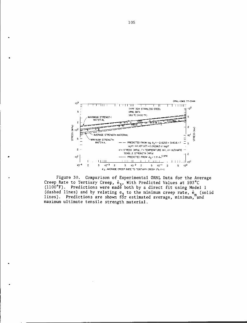
S 10^
F I I I II MM r
"V"^ AVERAGE STRENGTH MATERIAL^-MINIMUM STRENGTH
MATERIAL
J I II J L
10"
105
I I I llll I I I I I llllTYPE 304 STAINLESS STEEL
ORNL DATA
593 X (1100 °F)
ORNL-DWG 77-3144
"1 I I I I II
PREDICTED FROM log e3 = - 2.6253 + 3140.6/ Tlogor- 44.107 l//r+0.012963 t7 logcr
= STRESS (MPo), T- TEMPERATURE IK), tV= ULTIMATETENSILE STRENGTH (MPo)
PREDICTED FROM «3=1.11 em°'974I I I I III llll I I I III
10" 10"
«3, AVERAGE CREEP RATE TO TERTIARY CREEP (%/hr)
Figure 30. Comparison of Experimental ORNL Data for the AverageCreep Rate to Tertiary Creep, e_, With Predicted Values at 593°C(1100°F). Predictions were made both by a direct fit using Model 1(dashed lines) and by relating e_ to the minimum creep rate, e (solidlines). Predictions are shown for estimated average, minimum, andmaximum ultimate tensile strength material.

w IO2
10' -
10'
"1 I I I I llll
593 °C (1100 °F)
106
1 llll llll T ~T TTl0.977LINES PREDICTED FROM /5S = 0.752 /,
log /, = 5.716 - 3915 / T logo-+ 32.60 Ul T- 0.007303 U logo-ct = STRESS (MPo)
T = TEMPERATURE (K)
c7» ULTIMATE TENSILE STRENGTH (MPo)
ORNL-DWG 77-3146
TTTTT
- 5
- 2
— CO
TYPE 304 STAINLESS STEEL
° • 593 °C (1100 °F). o • 649 °C (1200 °F)
FILLED SYMBOLS-HEAT 8043813, 25-mm PLATEOPEN SYMBOLS-HEAT 972796, 51-mm PLATEPOINTS REPRESENT EXPERIMENTAL DATA
SOLID LINES-HEAT 9T2796DASHED LINES-HEAT 8043813
649 °C (1200°F)
- 2
I I llll J I I I J J I I I I I 10°
10' 10° 10"
/SS,TIME TO TERTIARY CREEP (0.2% OFFSET) (hr)
Figure 31. Comparison of Experimental Data With Predicted Valuesof Time to the Onset of Tertiary Creep at 593°C (1100°F) and 649°C(1200°F). Predictions are shown for heat 8043813 (a strong heat) andfor heat 9T2796 (a weak heat).

= 2o.
5
co 102
107
ORNL-DWG 77-3147
2"1 TT" "I I I I I I III I I I llll 1 I I I I I IILINES PREDICTED FROM e3=1.11 ej1574log em* -2.765 + 3346/7" logcr-51.84 t7/7> 0.01616 U logcr
0" = STRESS (MPo)
T = TEMPERATURE (K)
U = ULTIMATE TENSILE STRENGTH (MPo)
I I I I III
TYPE 304 STAINLESS STEELo • 593 °C (1100 °F)D • 649 °C (1200 °F)
FILLED SYMBOLS-HEAT 8043813, 25-mm PLATEOPEN SYMBOLS-HEAT 972796, 51-mm PLATEPOINTS REPRESENT EXPERIMENTAL DATA
SOLID LINES-HEAT 9T2796DASHED LINES-HEAT 8043813
J I I I llll J
io1 £
J L
2 10~3 2 5 10"* 2 5 10"1
e3, AVERAGE CREEP RATE TOTERTIARY CREEP (%/hr)10u
Figure 32. Comparison of Experimental Data With Predicted Valuesof Average Creep Rate to the Onset of Tertiary Creep at 593°C (1100°F)and 649°C (1200°F). Predictions are shown for heat 8043813 (a strongheat) and for heat 9T2796 (a weak heat).

108
and 38, page 103, are simpler and rely upon the more widely available
data for e are t , they are preferred.
Analogous to the development of Eqn. 34, page 90, above, Eqns. 38 and
39, page 103, can be combined to yield a direct expression for e, as a
function of U, a, and T as
190 7 IIloge3=2.105 ^p-loga- 14.273 j +0. 0060869 Ulog a. (42)
Equations 40 and 41, page 103, yield an expression of the form
e3= 0.835 em°-974 t 0.977 . (43)
Figures 33 and 34 compare results obtained using Eqns. 35 and 36, page 90,
and 43 to estimate e withexperimental data for heats 9T2796 and8043813.
As with the plasticity resource, the predictions appear to accurately
reflect trends in the data, although the uncertainty is again large.
For type 304 stainless steel the analyses in Refs. [50-52] treated
data for creep strain only, and did not include the instantaneous
strain incurred upon loading. In many cases, however, the only available
measure of ductility is the total strain (creep plus loading) to rupture,
et- Fortunately, the quantity e can be treated in the same fashion as
was e in Eqn. 33, page 89. Thus, one can write
•L = G t„ . (44)-e
't ~ "r
where £ = e /t . Thus,t t r '
1-e
ret = G t . (45)

109
ORNL-DWG 77-3148
STRESS (ksi)
30 40 50
LINES PREDICTED FROM
.j-0.76 *„°-9M /r0'968HEAT 9T2796
HEAT 8043813
TYPE 304 STAINLESS STEEL
593"C (1100'F I
POINTS ARE EXPERIMENTAL
DATA
o HEAT 9T2796 25-mm AND
51-mm PLATE
-• HEAT 8043813 25-mm PLATE
150 200 250 300 350 400
STRESS (MPo)
Figure 33. Comparison of Experimental Data With Predicted Valuesof Creep Strain to the Onset of Tertiary Creep at 593°C (1100°F).Predictions are shown for heat 8043813 (a strong heat) and for heat9T2796 (a weak heat).

IO2
go_
or<
p 10'
10° L
110
STRESS (ksi)
10 20
ORNL-DWG 77-3149
30
TYPE 304 STAINLESS STEEL649°C (1200°F)
POINTS ARE EXPERIMENTALDATA
o HEAT 9T2796 25-mm AND51-mm PLATE
a HEAT 8043813 25-mmPLATE
50
Q<S o
// o^„ 0
// « o// «»
// o//
// ° *h r//oo'o
' LINES PREDICTED FROM
1 ,3-0.76 J.*9"HEAT
, 0.968' r
9T2796
HEAT 8043813
100 150
STRESS (MPo)
200
Figure 34. Comparison of Experimental Data With Predicted Valuesof Creep Strain to the Onset of Tertiary Creep at 649°C (1200°F)Predictions are shown for heat 8043813 (a strong heat) and forheat 9T2796 (a weak heat).

Ill
Sikka and Booker [18] have applied this method to data from the US,
NRIM, and BSCC data mentioned last chapter. However, since Eqns. 44
and 45 are independent of ultimate tensile strength, all NRIM and BSCC
available data were used rather than only those for which corresponding
ultimate tensile strength data were available. Table XXX summarizes
the results from Ref. [18] for type 304 stainless steel, including
separate analyses of data for individual product forms for which a
significant amount of data were available. No noticeable effects due
to product form were observed. Figure 35, taken from Ref. [18],
illustrates the results. The top row of plots in Figure 35 shows the
results obtained by fitting Eqn. 44, page 108, tothe data for e . The solid
line was determined by a least squares best fit, while thedashed lines were
determined by adding or subtracting 2 x SEE (Table XXX) in log e from
the mean values. The lower row of plots in Figure 35 shows data and
predictions for e as a function of t . Solid lines and dashed lines
were obtained merely by multiplying the solid and dashed lines in the
upper row by t . The fit to the data is quite good.
Interpretation of Ductility Predictions
Although data for rupture ductility are widely available, the
processes occurring during third-stage creep (grain boundary cracking,
etc.) that lead to rupture are highly variable. As a result, variations
in rupture data can be especially large [35,57]. If one views rupture
as a kind of instability, it is reasonable to expect that the material
condition at the onset of this stability is a more fundamental property
than the condition after its occurrence [35]. These considerations

112
TABLE XXX
RELATIONSHIP BETWEEN AVERAGE STRAIN RATE TO RUPTURE
AND RUPTURE LIFEa
Number 104-hrof Regression Creep Total
Data Data Temperature CoefficientsSEE-
r2 ElongationSource Product Points TO (°F) G -£ (log er) (%) C*J
BSCC Tube 13 600 1112 1.69 -1.11 0.144 95.74
BSCC Tube 23 625 1157 1.81 -1.17 0.127 98.08
BSCC Tube 13 650 1202 1.82 -1.11 0.186 94.98
NRIM Tube 32 600 1112 2.19 -1.22 0.138 96.16
NRIM Tube 32 650 1202 2.46 -1.30 0.126 98.54
NRIM Tube 40 700 1273 2.41 -1.30 0.249 95.77
NRIM Tube 27 750 1383 2.20 -1.25 0.274 89.24
US Tube 22 593 1100 1.46 -1.05 0.194 92.81
US Tube 53 649 1200 1.73 -1.10 0.267 90.40
US Tube 5 732 1350 1.03 -0.93 0.248 88.71
BSCC Bar 15 550 1022 1.52 -1.14 0.105 99.11
BSCC Bar 13 600 1112 1.47 -1.05 0.256 95.27
BSCC Bar 14 650 1202 1.35 -1.00 0.111 99.17
BSCC Bar 4 700 1293 1.62 -0.92 0.154 97.56
US Bar 14 538 1000 1.73 -1.22 0.060 99.60
US Bar 5 565 1050 1.72 -1.23 0.065 99.61
US Bar 16 593 1100 1.50 -1.13 0.099 99.04
US Bar 35 649 1200 1.57 -1.06 0.159 98.49
US Bar 15 704 1300 1.52 -1.07 0.226 97.05
US Bar 12 732 1350 1.72 -1.06 0.159 96.26
us Bar 9 760 1400 1.50 -1.05 0.178 98.52
us Bar 10 816 1500 1.42 -1.04 0.178 97.67
BSCC Combined 15 550 1022 1.52 -1.14 0.105 99.11 9.12
BSCC Combined 26 600 1112 1.53 -1.08 0.202 96.13 16.22
BSCC Combined 23 675 1157 1.81 -1.17 0.127 98.08 13.49
BSCC Combined 27 650 1202 1.48 -1.02 0.170 97.17 25.12
BSCC Combined 4 700 1293 1.62 -0.92 0.154 97.56 87.10
fclRIM Combined 10 550 1022 1.90 -1.16 0.087 97.54 18.20
NRIM Combined 10 575 1067 1.74 -1.08 0.163 95.47 26.30
NRIM Combined 41 600 1112 2.17 -1.21 0.153 94.84 21.38
NRIM Combined 34 650 1202 2.49 -1.31 0.126 98.51 17.78
NRIM Combined 40 700 1293 2.41 -1.30 0.249 95.77 16.22
NRIM Combined 27 750 1383 2.20 -1.25 0.274 89.24 17.78
US Combined 17 538 1000 1.61 -1.17 0.086 99.29 8.51
US Combined 5 565 1050 1.72 -1.23 0.065 99.61 6.31
US Combined 44 593 1100 1.49 -1.08 0.181 95.86 14.79
US Combined 91 649 1200 1.60 -1.06 0.231 95.21 22.91
US Combined 26 704 1300 1.59 -1.04 0.266 95.75 26.92
US Combined 17 732 1350 1.35 -0.97 0.226 90.99 29.51
US Combined 9 760 1400 1.50 -1.05 0.178 98.52 19.95

1.13
TABLE XXX (continued)
Number 10 -hrof Regression Creep Total
Data Data Temperature Coefficients SEE Rz ElongationSource Product Points X°c) (*FT G -e (log e ) (%)
US Combined 21 816 1500 1.58 -1.02 0.254 95.03 31.63
9. •
Average strain rate to rupture, e , and rupture life, t , have beenrelated by e = Gt ~e r
t r
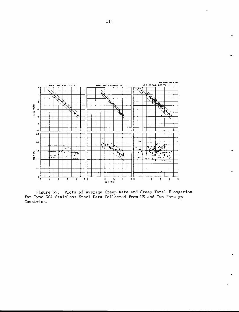
-1
-5
2.5
BSCC TYPE 304 (1202 *FI
N
«,
V ^
\\
>
-
*» '•
\ ^V9>•
^y "\°N
x* ^V S
N
^
«e
e
-w— ~B—' • i
#
ae
114
NRIM TYPE 304 (1202 •F)
*>;\
»^ v
> K' ^
%r«9\
-,
N,^
"JV v Sv
^> "»V
' ^ .;••
'
5 0 1 2 3
log /, (hr)
ORNL-DWG 76-4030
US TYPE 304 (1200-F)
\ 'W~- \ ^
E^ V
I V
tfl^i^?K
\« < \
A %•'k.
\
.
"
— r- -.
• • 1•
*
<!
O
. '. 1 » »9*~
S
1
9
• ,et
f
e
Figure 35. Plots of Average Creep Rate and Creep Total Elongationfor Type 304 Stainless Steel Data Collected from US and Two ForeignCountries.

115
suggest the use of the strain to onset of tertiary creep, e , as a
criterion of creep ductility.
Grant et al. [57,58] have suggested the use of e3 as a criterion,
referring to it as the "true" creep elongation. Booker and Sikka [51]
have discussed the advantages of e3 for design application. The major
advantage to the use of e, in design is the prevention of tertiary
creep and the associated cracking, void formation, and other
instabilities. Also, most currently used design creep strain-time
equations are valid only for the first and second stages of creep, so
that e3 represents the maximum amount of strain that can be predicted
from these equations. The cutoff point for the validity of these
equations for a constant load, isothermal situation could also be
located simply by knowing the time to tertiary creep. However, for
variable load conditions, previous results [8,9] have shown the
behavior of this material to be adequately described by the hypothesis
of strain hardening [12]. This hypothesis assumes that, under a given
load-temperature condition, the instantaneous strain rate—and thus the
instantaneous material condition—depends only on the previously
accumulated strain. Booker and Sikka [51] present results which
indicate that e3 is indeed relatively insensitive to the effects of
variable loads—depending only upon the instantaneous stress and
temperature at the onset of tertiary creep. Therefore, the strain
to tertiary creep might be a more meaningful criterion for variable load
conditions than the time to tertiary creep. In the next chapter, the
predicted values of e. will be used in the development of a creep
strain-time equation for type 304 stainless steel. Thus, it is seen

116
that a knowledge of the quantity e, can be very useful in design
applications—both as a measure of usable ductility and as a cutoff
point for creep strain-time temperature.
The plasticity resource, e , was first introduced [59,60] by Soviet
investigators who viewed it as an approximation to the creep strain to
tertiary creep, e,. This approximation was used to alleviate shortages
in available data for the quantity e3 itself. Goldhoff [61] has
disputed the general validity of this approximation, although recent
work [51] indicates that the approximation is fairly good for type 304
stainless steel. Actually, it can be shown [52] that e and e are
related by
es =̂(e3 -ep) (46)where e is the transient creep strain (see Figure 1, page 6). The
exact relationship thus depends upon t , t-» and e .
Several investigators [62-65] have discussed the possibility that
e is a material constant, independent of stress and temperature (and
thus of rupture life and strain rate). While some theoretical work
has been done [62], the conclusion that e is constant has been largely
based on the Monkman-Grant relationship [55] . That equation, however,
is essentially empirical, although similar relationships have been
defended theoretically [66,67]. The current results however indicate a
small but significant dependence of e on stress (nonunity slope in the
Monkman-Grant equation), and a definite dependence upon temperature. A

117
temperature dependence has also been observed by other investigators
[68-70]. Thus, one must conclude that e is not a fundamental material
constant, but is in some cases a reasonable approximation to e3.
Trends in Behavior
Figures 36 and 37 illustrate predicted trends in the value of e3
with variations in stress, temperature, minimum creep rate, and ultimate
tensile strength obtained using Eqn. 43 from page 108. For a given
heat of material, e, increases with increasing temperature from 482°C
to 704°C; while it decreases with decreasing stress or minimum creep
rate. Trends in e with variations in ultimate tensile strength (U)
are slightly more complex, although smaller. At a given stress, e3
generally decreases as U increases up to some high stress level, when
the trend is reversed. The relationship between U and e3 over the range
of creep at a constant minimum creep rate is a strong function of
temperature. Predicted trends in e are similar, although the values are
generally slightly higher than those for e_. The above trends are
clearly born out by experimental data, except for the variations with
ultimate tensile strength, which are so small that they are obscured
by the scatter in the data.
It will be seen in the next chapter that these predictions of trends
in e3 can be important in predicting general trends in creep deformation
behavior.

118
Kl"10 10
STRESS (kill
30 40 90 •0 TO
1 1 1 jA 1 1
Ay9*3* C tltOCF)
4
/A
A/
/
/ /
' /
m° /
/1< /
// |7-4«2'C (*O0*F>
// ,•/,
// /
/ *
' y
m-*
/j//
/
/
/
// /
// 11II
1 / Lll
ST
•es REP«
VAIN TO
IESENT
TERTIAR1
•REDICTI
f CREEP
0 VALUE
(NO OF
S OF TH
PSETI
E
io-«
f //SOI
DA
LID LINE
SHED LIN
l-AVERMES-MINIM
>E STREN
UM STRE
*TH MATN«TH Mil
ERIALTERIAL
DO HO goo
STRESS (MR*)
MO 400 490
Figure 36. Predicted Trends in the Strain to the Onset of TertiaryCreep (No Offset) as a Function of Stress.

10'
BQ.
P10°or
io-1 =—- ^^ —=• p -
<
119
ORNL-DWG 77-4172
- 1 1 I I 1 I T T 1 1 1 T 1 r^~r T 1 T T T-
r-
'04* C (13(X3 •F ) .
-
.-—;^**--
ll K i^,^_^ -
^' -
-
a >82»C (9( X) F
I
TYPE 304 STAINLESS STEEL
EPRESENT PREDICTED VALUES OF THETO TERTIARY CREEP (NO OFFSET)
INES-AVERAGE STRENGTH MATERIAL
- LINES R
-
STRAIN
SOLID L
1 _L 1 1 1 1 1 1
DASHED
, I
LI
_LJME
,1S
I
-MINIMUM
1 ,STRENGTH MATERIAL
ililil 1 I Ii 1IO-2KT4 10"3
e„, MINIMUM CREEP RATE (%/hr)
1CT2icr6 ro-8 KT1
Figure 37. Predicted Trends in the Strain to the Onset of TertiaryCreep (No Offset) as a Function of Minimum Creep Rate.


CHAPTER IV
ANALYSIS OF CREEP STRAIN-TIME BEHAVIOR
As stated in the Introduction, elevated temperature inelastic
design requires an expression for creep strain as a function of time
(t), stress (a), and temperature (T). Such an equation can also be
used to estimate the time allowed by the ASME Code Case 1592 [49]
restriction that the inelastic strain be limited to 1% and for
inelastic analyses. Methods for relating creep strain to time under
constant load (or stress), isothermal, uniaxial conditions, include
the following:
1. The times to accumulation ofgiven amounts of creep strain (t )
can be analyzed by techniques similar to those commonly used for rupture
life data. This method was used to describe data for Incoloy Alloy 800
(Grade 2), Inconel Alloy 625 (Grade 2), and 2 1/4 Cr-1 Mo steel by Roberts
and Sterling [71]. Using a series of strain levels and interpolating
between them, one can then reconstruct an entire creep curve. This method
suffers from the fact that it does not yield an expression for the creep
strain rate, which is required in design calculations. It can be used to
generate isochronous stress-strain curves such as those given in ASME Code
Case 1592 [49]. It should be noted that the particular method used by
Sterling [72] for Alloy 800 and 2 1/4 Cr-1 Mo steel assumed an equation
relating strain level to time and thus analytically "tied together" the
various strain levels. The Sterling equation can yield an expression
for creep rate as well as for creep strain.
121

122
2. A second possibility consists of using empirical relationships
among creep strain-time properties and better-established properties
such as rupture life or minimum creep rate. These relationships
generally involve equations similar to Eqns. 29-33, page 89, and 34,
page 90, except that they might relate t to^or totr [52]. Other
investigators [73-75] have proposed stress-based correlations, relating
the stress to cause x% strain in a given time to the stress to cause rupture in
that time. Such relationships again do not yield estimates ofcreep rate.
3. A method that has found some use is the parametric approach of
Rabotnov [76]. At a given level of total strain (e) (loading plus
creep), this parameter is given by
<{>(e) = a(l + at") (47)
where a and t are again the stress and time, <$> is the parameter, a is a
constant, and n is a constant whose value is about one-third. One can
use monotonic stress-strain curves (t = 0) to determine the value of <J>
at various strains, from which a can be determined from creep curves by
assuming n = 1/3 and solving Eqn. 47 to yield
a=(|- l)t 3. (48)
Since a is supposedly independent of a and t, only one point from one
creep curve should be required to determine a at each temperature.
Alternatively, the values of <j>, a, and n can be determined by least
squares fits to creep data [77].
4. The most popular method for design applications in recent years
has involved the use of creep equations, i.e. an analytical expression

123
for creep strain as a function of time, stress, and temperature. Since
these equations can generally be differentiated to yield expressions
for creep rate, they are the more useful for design purposes than the
above methods. Moreover, a creep equation can be more easily related
to the actual microstructural processes occurring during creep. This
method is thus the most useful both for practical design applications
and for fundamental studies of material behavior. Therefore, it is this
method that will be adopted here.
Methods for Development of Creep Equations
In general, the creep strain, e , is given by e (a, t, T). Two
basic methods for evaluation of this function have been proposed. The
first method, discussed by Penny and Marriott [35], assumes that the
functional dependence of e upon a, t, and T is separable such that
ec = £1(a)f2(t)f3(T) . (49)
Such a separation simplifies analysis procedures, but it may place an
undue restriction upon the flexibility of the equation to describe
material behavior.
The method that has recently been applied with some success
[29,38,78] involves first describing individual creep curves by a
strain-time equation. The parameters in this equation are then
themselves expressed as functions of stress and temperature. This
approach allows considerable flexibility and will be used here;
however, a new method for evaluating the stress and temperature
dependence of the equation parameters is proposed which alleviates

124
certain shortcomings in previous {29,38,78] evaluations. In particular,
the analyses for t , e , t , and e_ reported above are utilized in the
development of the creep equation. The resulting creep equation thus
allows a prediction of heat-to-heat variations in creep strain-time
behavior as it is reflected by ultimate tensile strength (U).
Choice of Strain-Time Equation Form
For the purposes of a design equation, it is necessary that the
creep equation be valid only through primary and secondary creep, since
design rules [49] preclude the onset of tertiary creep in service.
Fortunately, type 304 stainless steel exhibits almost exclusively
classical creep curves (as shown in Figure 1, page 6), further
simplifying the choice of strain-time equation form. A large number
of equation forms have been proposed as reviewed in Refs. [79-82]. Of
these, the most widely popular are listed in Table XXXI, following the
listing of Garofalo [80]. The most commonly used forms for austenitic
stainless steels have been the so-called single and double exponential
equations, given by
ec = e [1 - exp(-rt)] + e t (50)
and
ec = ex[l - exp(-st) + et[l - exp(-rt)] + ej: . (51)
Equation 50, first introduced empirically by McVetty [83] gained
acceptance for type 316 stainless steel through the work of Garofalo
et al. [84]. Subsequent investigators have applied Eqn. 50 to a variety

EquationName
Logarithmic
Power Law
Exponential
Linear
TABLE XXXI
SOME COMMON CREEP STRAIN-TIME RELATIONS
Equation Form
e = alnt + c
me = e + 3t
jor e = e + 3t + kt
,1 -rtN. ' *= eQ + et(l - e ) + egt
or e =-rt,= e0 + et(l - e )+ex(l - -st. • .e )+est
T/T,m
0.05-0.3
0.2-0.7
0.4-0.6
Materials
Al,Ag, Au,Cd,Cu,Mg,Ti-Steel, Al-10% Cu,and Cu-3% Ag
Al,Ag,Brass,Cd, Cu,Iron and Steel, Mg,Mg-2% Al, Ni, Pb, Pt,Sn, and Zn
Ferritic and Stainless
Steel
e = e„ + e to s
0.96-0.99 Al,Au,Cu, and 6-Fe
Cn

126
of materials, and considerable attention has been given to the meanings
of and interrelationships among the parameters e , r, and e [85-95].
In fact, some investigators [90,92-94] have extended the validity of the
equation through tertiary creep by the addition of a positive exponential
term. Although Eqn. 50, page 124, has been widely applied, it often
underestimates the creep rate in the initial part of the creep curve
[29,89-95]. Blackburn [29] proposed Eqn. 51, page 124, where the second
exponential term (the so-called "fast transient" term) was added to increase
the accuracy ofthe equation in the initial stages. It should be noted,
however, that Wilshire and co-workers [89-94] fit Eqn. 50 to experimental
data in the form
e = eL + et[l - exp(-rt)] + e t (52)
where e is the instantaneous strain incurred upon loading and thus
corresponds to the strain at zero time. In fitting this equation, eT
was generally overestimated, resulting in the situation shown
schematically in Figure 38. The curve fitting procedure used by
Blackburn [29] suffers from a similar shortcoming. On the other hand,
if one subtracts the loading strain and fits creep strain only using
Eqn. 51, the equation form itself forces a better fit in the initial
stages, since e is always zero at t = 0. Thus, the problems incurred
with fitting the single exponential equation were probably due as
much to the particular curve-fitting procedures employed as to
shortcomings in the equation form. For design applications, any
additional precision obtained by adding the second exponential term is
probably not justified by the increase in the complexity of the model.

<crHcn
127
ORNL-DWG 77-3150
EXPERIMENTAL DATA
FITTED CURVE
TIME
Figure 38. Schematic Diagram Showing Results of Fitting Eqn. 49Directly to an Experimental Creep Curve.

128
It should be noted the "double exponential" equations developed by
Blackburn [29] for types 304 and 316 stainless were used to develop the
isochronous stress-strain curves in ASME Code Case 1592 [51]. These
equations have several shortcomings which are alleviated by the current
results, as will be shown below.
Recent results for 2 1/4 Cr-1 Mo steel [38] indicate the
applicability of a rational polynomial equation, which can be written as
e =t^T +emt (53)c 1 + pt m
where e is again the creep strain, t the time, e the minimum creepc m
rate, and C the limiting value of the transient primary creep strain.
The parameter p is related to the sharpness of the curvature of the
primary creep region. Preliminary results in the current analysis
indicated that Eqn. 53 could also beused todescribe individual creep curves
for type 304 stainless steel. Subsequently, an analysis for type 316
stainless steel [78] found the rational polynomial equation to be superior
to the exponential equations. Significantly, although both single and
double primary term exponential equations and single and double term
rational polynomial equations were studied, it was found in Ref. [78] that
the single rational polynomial equation was preferable due to its
inherent simplicity. At any rate, it appears justified to examine both
the exponential and rational polynomial equations in detail.
The Exponential Creep Equation
The exponential creep equationformwas first introduced [83,84,89-94]
on an empirical basis merely because its mathematical properties resemble

129
those of primary and secondary creep curves. Differentiating Eqn. 50,
page 124, one obtains an estimate of the creep rate, e , as
ec =etre"rt +em . (54)
Thus, the initial creep rate, e is given by
e = e r + e , ess")o t m L DJ
but e decreases exponentially and asymptotically approaches the minimum
creep rate. The contribution of the primary term approaches a maximum
value of e . The parameter r, often called the time constant, controls
the rate of decay of the transient contribution and thus is related to
the sharpness of curvature of the primary region of the creep curve. It
can easily be seen that these same basic comments apply to the double
exponential form of the equation.
Recently, this same equation has been derived by several
investigators on a phenomenological basis. Webster et al. [95] begin
by assuming that primary and secondary creep obey first-order kinetics,
de
dlT = " (*c " Vr ' c56)
Integrating this expression twice yields Eqn. 50. Equation 51, page 124
can be derived upon the assumption that two separate mechanisms operate
independently, each obeying its own first-order kinetics.
Mejia et al. [96] recently presented a similar phenomenological
approach through which a variety of equation forms can be derived.

130
Their basic equation was
o^ =-8Ce)Cec-en) . (57)
It should be noted that Eqn. 56 is merely a form of Eqn. 57 with
g(e) = r.
Soviet investigators [87,88] have also derived arelationship from an
independent phenomenological approach. They assumed that amaterial
contains randomly distributed sources of deformation, each of which requires a
certain stress for activation. Once activated, a source produces a mean
amount of deformation J in a mean time of t. Each source then ceases to
act due to the buildup of internal stresses or work hardening. At high
enough temperatures, the source can recover in a mean time T, after which
it can be reactivated. Next, it was assumed that both source activation
and source recovery obey first-order reaction kinetics, so that
.Jl = _vN +W(N - N) (58)dt v o J
where v = 1/t, w = 1/t, N is the number of sources initially present and
N is the number of sources available for activation at a given time.
Equation 58 can be integrated with N = N for t = 0 to give
N=N -JL_ [1 - e-(v+w:,t] +N e-(v+w)t . (59)O V + W J 0
The total number of sources actually activated in a time, t, is then
given by
N = / t r Ndt . (60)3. O

131
Noting that the total creep strain, e , occurring in time, t, is given
by 6N , Eqn. 59 can be integrated to yieldcl
ec = elvw t+_rl_(i_e-(v+w)t)
v+w , -.2(v+w)
(61)
where e, is the maximum strain that could be incurred in the absence of
any recovery (i.e. e, = 6N ). Equation 61 is clearly of the same form
as Eqn. 50, page 124, except that the equation parameters are now explicitly
defined in terms of e,, v, and w.
The Rational Polynomial Creep Equation
The properties of the rational polynomial creep equation given in
Eqn. 53, page 128, are reviewed in detail in arecent report by Hobson and
Booker [97], but will be briefly described here for completeness. While
not as widely used through the years as the exponential equations, the
rational polynomial equation is not new. In fact, an equation
equivalent to Eqn. 53 but without the linear secondary term was used by
Freudenthal more than forty years ago [98]. The equation was introduced
in its present form by Oding more than twenty years ago [99]. The current
popularity of the equation began with the analysis reported in
Ref. [38] for 2 1/4 Cr-1 Mo steel.
Clearly, the parameter C in the national polynomial equation is
analogous to e in the single exponential equation, while e is the
minimum creep rate in both cases. Differentiating Eqn. 53 one
expresses the creep rate, e , as
e = CPt +em , - (62)(i+ptr

132
while the initial creep rate is given by
e = Cp + e . (63)o r m *• •*
The parameter p is related to the rate of approach of the creep rate from
e to e . Figure 39 summarizes the properties of the rational polynomial
equation.
Equations 50, page 124, and 53, page 128, being ofdifferent form,
cannot bemade identically equal, but they canbe made to approximate one
another within the accuracy of engineering creep data. To do so, one first
lets e be the same in each equation, and then lets c = e . Then, the
two equations can be set equal at any point along the curve to determine
the relationship between p and r. A logical choice of this point is
the point at which half the transient strain has been exhausted. Calling
the time at this point t*, it can easily be verified from Eqn. 53 that
t* = — . Equating Eqns. 50 and 53 at t = t* yields
p = 1.44r . (64)
Thus, the single exponential and rational polynomial equations can be
used almost interchangeably. Interestingly, Eqns. 63 and 64 imply that
the rational polynomial equation yields a slightly higher initial creep
rate than the exponential equation, other things remaining the same.
The rational polynomial creep equation is probably best viewed as
a simple, flexible means of empirically representing experimental creep
data. However, it too has been derived from various formulations of
creep behavior. Oding [81,99] derived the equation form based on a
self-diffusion theory of creep. The equation was also derived [81]
on a phenomenological basis, as follows.

<cr
133
ORNL-DWG 76-3985R
END OF SECONDARY PORTION e=e3>t=t.
SLOPE « e
SINGLE RATIONAL POLYNOMIAL
CREEP EQUATION ec=-^r+emt
PRIMARY PORTION
•INITIAL SLOPE = Cp + e
TIME
m
Figure 39. Schematic Illustration of the Properties of the RationalPolynomial Creep Equation.
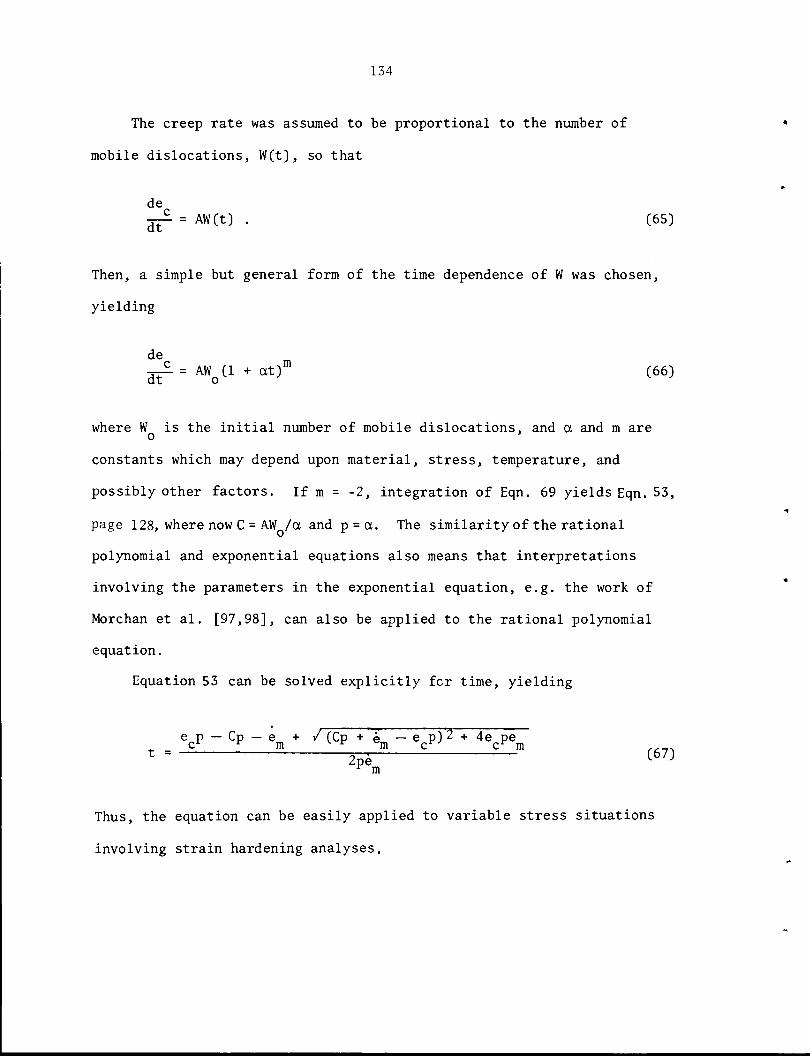
134
The creep rate was assumed to be proportional to the number of
mobile dislocations, W(t), so that
de
-^- =AW(t) . (65)
Then, a simple but general form of the time dependence of W was chosen,
yielding
de
-i-£- = AW (1 + at)m (66)dt o^ v J
where W is the initial number of mobile dislocations, and a and m areo '
constants which may depend upon material, stress, temperature, and
possibly other factors. If m = -2, integration of Eqn. 69 yields Eqn. 53,
page 128, where now C = AW /a and p = a. The similarity of the rational
polynomial and exponential equations also means that interpretations
involving the parameters in the exponential equation, e.g. the work of
Morchan et al. [97,98], can also be applied to the rational polynomial
equation.
Equation 53 can be solved explicitly fcr time, yielding
ecP - Cp - em ♦ /(Cp + em - ecp)2 + 4ecpemt = —„ (67)
r m
Thus, the equation can be easily applied to variable stress situations
involving strain hardening analyses.

135
The analytical flexibility and simplicity of the rational polynomial
equation give it a definite advantage over the exponential equation.
Moreover, the equation is much more economical to apply in terms of
computer time used in performing design calculations. Our analyses
showed that the equation does very good job of fitting experimental creep
data. Therefore, the rational polynomial form was chosen as the basic
strain-time equation to use in developing a creep equation for type 304
stainless steel.
Fits to Experimental Curves
The rational polynomial equation can be fitted to experimental
curves by various least-squares and graphical techniques, as described
elsewhere [97]. In general, the least-squares techniques will yield the
most objective fit. However, in the current analysis, many low-stress
and low-temperature tests were used in which the amount of strain incurred
was so small compared to the accuracy of the strain-measuring equipment
employed that a great deal of scatter occurred in the data. In order
to avoid drawing wrong conclusions fromleast-squares fits due to this
scatter, the semigraphical approach described by Bunatyan [81,100] was
employed.
Bunatyan [100] showed that if one chooses three points (t,,e,),
(t2,e2), (t,,e_) from an experimental creep curve, the values of p and
e can be found bym
"l-^K e2J +t3- h^H \ ^2 *1p = " - — (68)
12, a,tZ=t7 Ce2 " e3> + 61 " 62

136
and
1e ="m (t, - t_)
ei e2+ e, — e.
[pt, pt2 1 2(69)
The value of C can then be determined by setting the prediction of Eqn. 53,
page 128, equal to the experimental strain at any point on the curve. In
the current analyses, we determined C at each of the above three points
and then averaged those values, although they did not vary greatly.
Figures 40-44 illustrate fits to experimental curves obtained using
this method.
Stress and Temperature Dependence of Equation Parameters
In other analyses [29,38,78] the stress and temperature dependence
of the creep equation parameters were evaluated as follows. First,
available experimental creep curves are individually fit using the chosen
equation form to yield a set of parameter values for each test. Then,
the individual equation parameters are themselves directly expressed as
functions of stress and temperature. Although this method has met with
some success, it suffers from several shortcomings, enumerated below,
and hereafter referred to as Objections 1-4.
1. The number of available creep curves is often quite small in
comparison to rupture and other data. The number of creep data can be
too small to adequately identify the dependence of the equation
parameters upon stress and temperature.
2. Experimental variations and complex interrelationships among
equation parameters can cause considerable scatter in the values of
these parameters. As a result, the correlations between these parameters
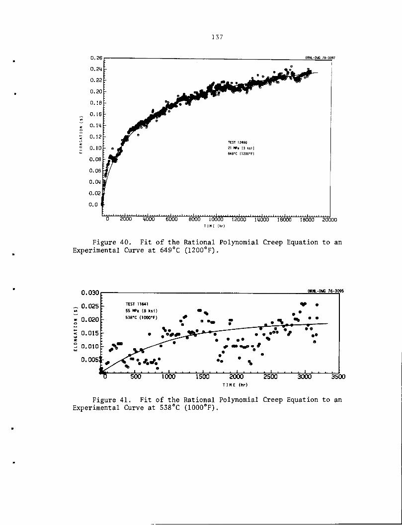
137
ORHL-DUG 76-3097
0 2000 14000 6000 8000 10000 12000 1"4000 16000 18000 20000TIKE (hr)
Figure 40. Fit of the Rational Polynomial Creep Equation to anExperimental Curve at 649°C (1200°F).
0.030
-. 0.025
- 0.020o
* 0.015Z
° 0.010UJ
0.005!r
TEST 11641
55 MPa (8 ks1)
538'C (1000'F)
i i—* * ' * • * * ' * * * • ' * * • *
2000
TIME (hr)
ORNL-DWG 76-3095
3000 3500
Figure 41. Fit of the Rational Polynomial Creep Equation to anExperimental Curve at 538°C (1000°F).

138
10000 15000
TIME (hr)
ORNL-DWG 76-3096
TEST 11596
83 MPa (12 ks1)
593'C (1100'F)
20000 25000
Figure 42. Fit of the Rational Polynomial Creep Equation to anExperimental Curve at 593°C (1100°F).

139
PW1L-PM6 7E--3W3
iooob 12000nioooI6000isooo 20000TIME (lir)
Figure 43. Fit of the Rational Polynomial Creep Equation to anExperimental Curve at 427°C (800°F).
8000 10000
THE (hr)
0M.-CW 76-3094
12000 14000 16000
Figure 44. Fit of the Rational Polynomial Creep Equation to anExperimental Curve at 482°C (900°F).

140
and the test conditions (a, T) can be very poor. This problem becomes
particularly large when extrapolation in one or more of the independent
variables is necessary.
3. Separate analysis of the equation parameters as functions of
stress and temperature can cause problems when the parameters are
recombined into a unified equation, since they are actually strongly
interrelated.
4. It is extremely difficult to account for heat-to-heat
variations using this method.
In the present investigation, an alternate method has been devised
to help overcome the above objections. One of the advantages of the
current equation form is the explicit minimum creep rate term. While
analytical fits of Eqn. 53, page 128, to experimental curves will in general
yield slightly different values of e than will graphical measurements, this
difference is insignificant in comparison to the overall uncertainty
in creep strain-time predictions. The approach used here has been to
use the analyses of minimum creep rate data from Chapter III of this
report to express e as a function of stress and temperature. Since
the creep curves were primarily from the ORNL data (Table VII,
page 14), the ORNL equation for e was used. Reiterating the results
of Chapter III, this equation is
log em =-2.765 +^|^log a-51^,84U +0.01616U log a (70)
where e is the minimum creep rate (%/hr), T the temperature (K), a the
stress (MPa), and U the ultimate tensile strength (MPa) at temperature
for a given heat of material at a tensile strain rate of 6.7 x io" sec ,

141
From Figure 39, page 133, it can easily be verified that the value
of C is given by
C = e - et, , (71)3 mo
where e_ and t, are the strain and time to the onset of tertiary creep
(first deviation from linear secondary creep). Again reiterating
results previously mentioned in this report, t_ and e_ can be found from
t, =0.685 t°'968 (72)3 r
and
where
,-,-,- 0.974 ,7^e3 =V^ = 1'11 6m » (73)
logt =5.716 -~^ logo* 3you _0.007303Uloga (74)
with t = rupture life and a, T, and U as in Eqn. 70. Equations 71-74
in turn yield
a -.en" 0-974 0.968 r7cne, = e_t, = 0.760 em t^ (75)3 3 3 m r
and
C-O.eSSt0-96^!.!!^0-974-^ • (76)r m m
Many previous investigators [84-87, 89-96], using the single
exponential creep equation, found the initial creep rate, eQ, to
be a constant multiple of em for a variety of materials. The time

142
constant, r, was also found to be a constant multiple of e exceptr m r
at low stresses in iron [95] and type 316 stainless steel [84].
Several such relationships were examined in the current analysis, the
one chosen as optimum being
, ., • 0.80e = 3.43 e , (77)
as illustrated in Figure 45. Since eQ is given by Cp + e , the
parameter p(hr_1) is given by
P=!2"P?L ' (78)
With the aid of Eqns. 70, page 140, 76-78, it is possible to evaluate the
entire creep equation from a knowledge of e and t for a given material,m r °
Predictions of Creep Behavior
The method described above allows an evaluation of the dependence
of the parameters C, p, and e upon stress, temperature, and relative
strength of a given heat of material (as reflected by the ultimate
tensile strength). Figure 46 illustrates the predicted behavior of
these parameters for the 51-mm thick plate of heat 9T2796 [25], a weak
heat. The predictions were made using values of ultimate tensile for
these heats of material from Refs. [25] and [27] respectively. The
experimental points represent values obtained by fitting individual
creep curves using the method described above.
Several points are apparent from Figures 46. First, the scatter
in the data is large (thus the second objection above to previous
evaluation procedures). Second, although the current equations were

ccx
(E
0_LU
143
ORNL DWG 77-8885
TYPE 304 STAINLESS STEEL
:
o
: Ojffl
:
<D
O
n
0*
[&j4
|8So(p
'
O
aA Vo
1 -41 -1 S -11 1 » i
LOG MINIMUM CREEP RATE (%/HR)
Figure 45. Relationship Between Minimum Creep Rate and InitialCreep Rate for Type 304 Stainless Steel.

ORNL-OWO 76-10220
STRESS (ksi)
(0 15 20 25
100 <50
STRESS (MPo)
(a)
250
ORNL-DWG 76-10219
STRESS (ksi)
10 15 20 25 30 35
100 150
STRESS (MPo)
(b)
250
Figure 46. Variation of the Rational Polynomial Creep Equation Parameters With Stress at ThreeTemperatures for Heat 9T2796, 51-mm Plate of Type 304 Stainless Steel, (a) Experimental data for theparameter C, with predictions from the creep equation; (b) experimental data and predictions for theparameter p.
4^
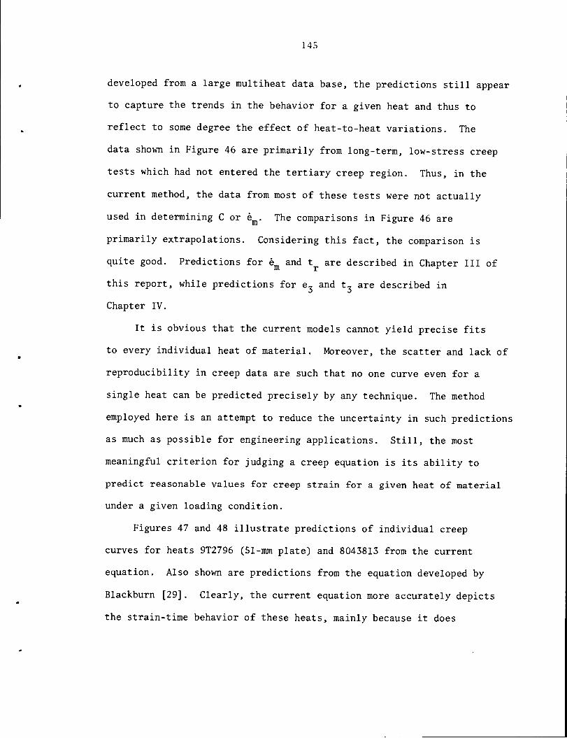
145
developed from a large multiheat data base, the predictions still appear
to capture the trends in the behavior for a given heat and thus to
reflect to some degree the effect of heat-to-heat variations. The
data shown in Figure 46 are primarily from long-term, low-stress creep
tests which had not entered the tertiary creep region. Thus, in the
current method, the data from most of these tests were not actually
used in determining C or e . The comparisons in Figure 46 are
primarily extrapolations. Considering this fact, the comparison is
quite good. Predictions for em and t are described in Chapter III of
this report, while predictions for e3 and t3 are described in
Chapter IV.
It is obvious that the current models cannot yield precise fits
to every individual heat of material. Moreover, the scatter and lack of
reproducibility in creep data are such that no one curve even for a
single heat can be predicted precisely by any technique. The method
employed here is an attempt to reduce the uncertainty in such predictions
as much as possible for engineering applications. Still, the most
meaningful criterion for judging a creep equation is its ability to
predict reasonable values for creep strain for a given heat of material
under a given loading condition.
Figures 47 and 48 illustrate predictions of individual creep
curves for heats 9T2796 (51-mm plate) and 8043813 from the current
equation. Also shown are predictions from the equation developed by
Blackburn [29]. Clearly, the current equation more accurately depicts
the strain-time behavior of these heats, mainly because it does
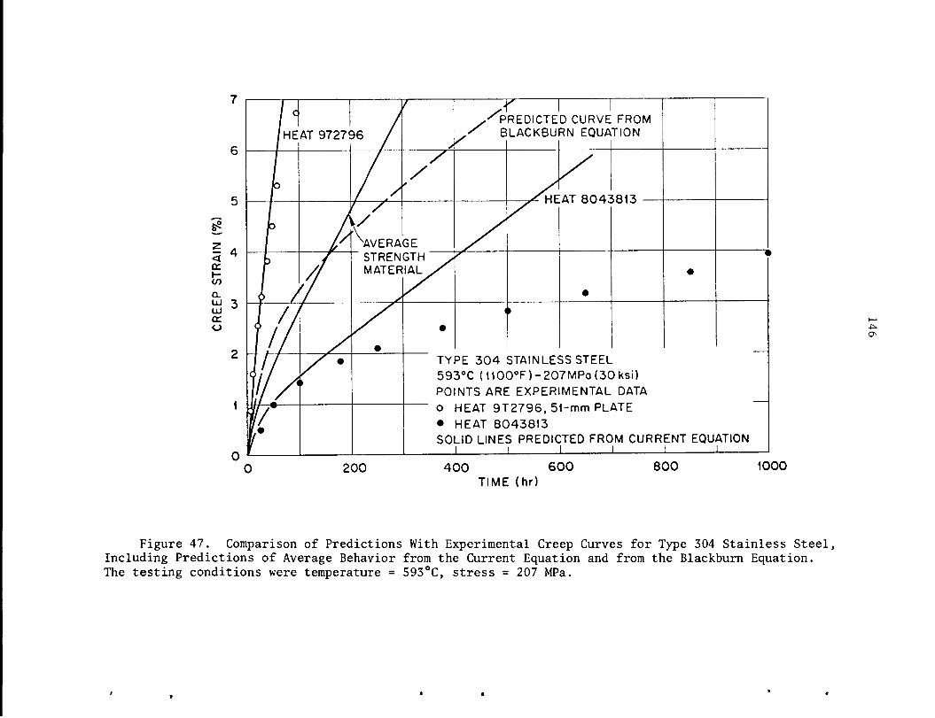
&s
<4crr-
</)
O.
uj 3UJcco
200
TYPE 304 STAINLESS STEEL
593°C (1100°F)-207MPa(30ksi)
POINTS ARE EXPERIMENTAL DATA
o HEAT 9T2796,51-mm PLATE
• HEAT 8043813
SOLID LINES PREDICTED FROM CURRENT EQUATION
400
TIME (hr)
600 800 1000
Figure 47. Comparison of Predictions With Experimental Creep Curves for Type 304 Stainless Steel,Including Predictions of Average Behavior from the Current Equation and from the Blackburn Equation.The testing conditions were temperature = 593°C, stress = 207 MPa.

*e
<cr\-
o_UJ
UJcro
147
TYPE 304 STAINLESS STEEL
.649 °C (1200 °F) - 69 MPa (10 ksi)
o HEAT 9T2796,51-mm PLATE• HEAT 8043813
POINTS ARE EXPERIMENTAL DATASOLID LINES PREDICTED FROM CURRENT EQUATION
o
2 3 4
TIME (103 hr)
Figure 48. Comparison of Predictions With Experimental Creep Curvesfor Type 304 Stainless Steel, Including Predictions of Average Behaviorfrom the Current Equation and from the Blackburn Equation With theTesting Conditions: Temperature = 649°C, Stress = 69 MPa.

148
reflect heat-to-heat variation whereas the Blackburn equation does not.
Figure 49 illustrates the ability of the current equation to predict
the range in creep behavior for this material.
Finally, the data used in establishing the current predictions
were almost exclusively from tests conducted at temperatures of
538°C (1000°F) and above. However, creep in this material has been
recognized as important in design [49] at temperatures down to
427°C (800°). The predictions must therefore be extrapolated downward
in temperature. Creep data at such low temperatures are primarily
from heat 9T2796. Comparisons between the predictions and data at
482°C (900°F) for this heat yielded generally good results at high
stresses, with the equation tending to underpredict the amount of
creep strain as the stresses were lowered. At 427°C (800°F) only
relatively low stress data were available. The creep strain occurring
under these conditions is significantly underpredicted by the current
equation. In fact, at these low stresses and temperatures the
dependence of creep strain on temperature appears to be markedly
reduced. As shown in Figure 50, this material can creep as much or
more at 427°C than at 482°C for the same stress. A close look at
Figure 17, page 71, indicates a possible trend toward a downward break
in the log a-log em isothermals (less stress dependence in e ) at low
stress even at 593°C and 649°C. These trends toward decreased stress
and temperature dependence at low stresses and temperatures may be
indicative of changes in creep deformation mechanism. This possibility
will be addressed in the next chapter.

60
50
149
ORNL-Owe 7*-t750
(a)
ORNL-DWG 76-97-18
TEMPERATURE- 593»C (1100 *F)'STRESS =241 MPa (35 ksi)
20 HEATS OF TYPE 304REANNEALED CONDITION. 0.5 hr AT 1065 *C (1950 *F)
PREDICTED
la) MAXIMUM Su
(A) AVERAGE Su
(<7) MINIMUM Su
100 200 300 400 500
TIME (hr)
600 700 800 900
(b)
Figure 49. Heat-to-Heat Variations in Creep Curves of SeveralReannealed Heats of Type 304 Stainless Steel, (a) Creep tests at241 MPa (35 ksi) and 593°C (1100°F). (b) Creep tests at 207 MPa(30 ksi) and 593°C (1100°F).

**
<crr-
00
0_UJUJoro
0.10
0.08
0.06
0.04
0.02
0
0
ORNL-DWG 76-10225
TYPE 304 STAINLESS STEEL
HEAT 9T2796, 51-mm PLATE
POINTS ARE EXPERIMENTAL DATA
o 482 °C (900 °F)
• 427 °C (800 °F)
LINE PREDICTED FROM CREEP EQUATION
AT 482 °C
4i
Q
4 5 6
TIME (IO3 hr)
8 10
Figure 50. Illustrative Comparison Among Creep Data at 482°C (900°F) and 427°C (800°F) andPredicted Behavior at 482°C.
On
O

151
Variable Load and Relaxation Behavior
Actual design applications will seldom involve simple constant-load
situations. Various system transients and other effects will result in
repeated changes of stress or temperature or both. Also, many loading
situations involve constant strain stress relaxation rather than constant
load creep straining. To be of full use, a creep equation must provide
some means of accounting for such situations. Little study has been
done of variable temperature behavior, but some data from variable load
tests are available.
It is beyond the scope of this investigation to undertake a study
of schemes for treating variable load creep behavior in this material.
Currently used constitutive relationships [8,9] suggest that the
hypothesis of strain hardening [12] be used to describe the variable
stress creep behavior of type 304 stainless. This hypothesis assumes that
the instantaneous strain rate at any stress and temperature is given
uniquely as a function of the stress, temperature, and accumulated
strain. Current rules [8,9] specify that this accumulated strain
includes creep strain only. Since the rational polynomial equation
can be solved explicitly for time as a function of strain [Eqn. 67,
page 134], it is a simple matter to apply the strain hardening approach.
Knowing the accumulated creep strain, one can solve the equation for
time at the given stress and temperature, thus locating a point on the
predicted creep curve for that stress and temperature. Creep then
proceeds along that curve until the stress or temperature changes again.
Figure 51 illustrates a prediction made from the current equation for
a variable load creep test for heat 8043813 [27], while Figure 52

2.0
1.6
55
z 1.2<trI-CO
CLUJUJ
cr 0.8o
0.4
0
0
152
ORNL-DWG 76-10230
7~
TYPE 304 STAINLESS STEEL
HEAT 8043813
649°C (1200°F) /"•
/ ^103 MPa
400
69 MPa
103 MPa
SOLID LINES-EXPERIMENTALVARIABLE LOADING DATA
DASHED LINES-PREDICTED FROMCREEP EQUATION USING STRAINHARDENING —
800 1200
TIME (hr)
1600 2000
Figure 51. Comparison Between an Experimental Variable Load CreepTest for Heat 8043813 With Predicted Behavior Using the Current CreepEquation and the Hypothesis of Strain Hardening.

160
120
o
oo 80
crr-
oo
40
ORNL-DWG 76-10231
•• •-
TYPE 304 STAINLESS STEEL
HEAT 9T2796, 25-mm PLATE
593 °C (1100 °F)
••^•Sk.^•^••>^^--
^•^..:•-••#^^
POINTS AND SOLID LINES - EXPERIMENTAL RELAXATION DATA
DASHED LINES PREDICTED FROM CREEP EQUATION USING STRAIN HARDENING
mi i i i nun i i i Mini i i i mini
20
_ <n
oooo
10orh-
,-210
-110 10L IO1 10' 10;
TIME (hr)
Figure 52. Comparison of Two Experimental Relaxation Curves for Heat 9T2796 at 593°C WithPredicted Behavior Using the Current Creep Equation and the Hypothesis of Strain Hardening.

154
illustrates results obtained in predicting relaxation behavior for the
25-mm plate of heat 9T2796 [101]. The predictions show good agreement
with the experimental data.
Isochronous Stress-Strain Curves
One of the most useful forms of displaying creep strain-time
behavior is the isochronous stress-strain curve. Various methods exist
for the construction of such curves, such as that summarized in
Ref. [71].
Equation 50, page 124, with the constants e, C, and p defined by
Eqns. 70, page 140, 76, page 141, and 78, page 142, respectively, can
beused tocalculate the creep strain accumulated in a given time at a
given stress and temperature. Thus, from an estimate ofthe instantaneous
strain incurred upon loading, one can develop isochronous stress-strain
curves from the equation. This loading strain can be determined from
monotonic tensile stress-strain curves.
The monotonic tensile stress-strain behavior of this material can
be described by:
C'p'e(a - an) = - 5— + h e , (79)^O-'i+pemp' K J* p *
where a is the stress (MPa), e the plastic strain (cm/cm), and a corresponds
to the proportional limit. The value of aQ can be well estimated as
0.5 a ,where a is the 0.002 strain offset yield strength. The constant
n is approximately equal to 2586 MPa, while p is given by 500 C'. The value
of C" is determined by the criterion that o = a for e = 0.002.y P
Interestingly, Eqn. 79 is of the same form as Eqn. 53, page 128,

155
reflecting the great flexibility of this equation. Since a knowledge of
stress and Young's modulus yields the magnitude of the elastic strain,
Eqn. 79can be used to calculate the total strain corresponding to a
given stress. A full description of our analysis of stress-strain
behavior is given elsewhere [102].
Equations 53,page 128> and 79 were combined to calculate isochronous
stress-strain curves as shown in Figure 53. Average, maximum, and
minimum creep strength curves were calculated by using the corresponding
values of tensile strengthfrom Eqn. 22, page 72, for the ORNL data.
For all cases shown in Figure 53, the loading strains were calculated
using average yield strengths from Ref. [16] for as-received material,
to allow comparison with the results of Ref. [29]. Thus, all variations
shown are due to the effects of creep strength only.
Figure 53 shows that there are considerable differences between
the current results and those of Ref. [29]. Since the current method
allows one to calculate a series of isochronous curves for different
heats of material, it is generally expected to be more accurate for a
given heat of material. At 538°C (1000°F) and below, the results of
Ref. [29] sometimes fall even below the current minimum predictions.
However, based on available low temperature data (427-538°C),
our results are the more realistic of the two.
Finally, for comparison purposes, two alternate methods were used
to construct isochronous curves for the heat 9T2796 51-mm plate.
First, the times to accumulation of given amounts of creep strain
were analyzed by parametric techniques similar to those commonly used
for rupture data. This method is similar to the one described in

200
0.8 1.2
STRAIN (%)
ORNL-DWG 76-10226
(a)
Figure 53. Predicted Isochronous Stress-Strain Curves at 10 - and 10 -hr from the Creep Equationand the Rational Polynomial Equation for Average Stress-Strain Behavior. Shown are predictions forestimated average, minimum, and maximum ultimate tensile strength levels. Also shown are values fromisochronous curves constructed from the Blackburn equation. (a) 538°C (1000°F); (b) 593°C (1100°F);(c) 649°C (1200°F).
on
ON

200
ORNL-DWG 76-10227
AVERAGE STRENGTH MATERIAL
MINIMUM STRENGTH MATERIAL
MAXIMUM STRENGTH MATERIAL1
_LINES PREDICTED FROM CURRENT EQUATION
AVERAGE MONOTONIC
TENSILE CURVE
POINTS PREDICTED FROMBLACKBURN EQUATION
o IO3 hr105 hr
0
TYPE 304 STAINLESS STEEL
593 °C (1100 °F)
0.4 0.8 *-2STRAIN (%)
(b)
Figure 53 (continued)
1.6 2.0
CO
CO
ooUl
rr
CO
in

200ORNL-DWG 76-10228
LINES PREDICTED FROMCURRENT EQUATION
AVERAGE STRENGTH MATERIALMINIMUM STRENGTH MATERIAL
" MAXIMUM STRENGTH MATERIAL
POINTS PREDICTED FROMBLACKBURN EQUATION
0.8 12
STRAIN (%)
(c)
Figure 53 (continued)
— 25
— 20
-6 15
10
.— 5
2.0
co
COUJ
or
(-CO
cn00

159
Ref. [71]. No extensive modeling was attempted, although we did fit
several standard time-temperature parameters to data for 0.1, 0.25, 0.5,
1, 1.5, and 2% creep strain. The best results were obtained by a simple
Larson-Miller [45] parameter of the form
oij log a a2log tx = aQ + ^ + — , (80)
where aQ, o^, and a2 were estimated by least squares methods at each of
the above levels of creep strain. Equation 80 allows one to calculate
the stress that will cause a given amount of creep strain at a given
time and temperature. Using this stress, one can then use Eqn. 79,
page 154, and Young'smodulus to calculate isochronous stress-strain curves.
Finally, isochronous curves at 593°C (1100°F) were constructed using
a form of the Rabotnov parameter [76]. At a given level of strain
(loading plus creep), this parameter is given by
♦00 = o(l + at ' ) , (81)
where a and t are again the stress and time, (J) is the parameter and a is
a constant. We used stress values obtained from the above-mentioned
monotonic tensile stress-strain curves for <J>, and assumed a time exponent
of 1/3. Attempts at determining <j> and the exponent by least squares
methods, such as was done in Ref. [77], yielded poor results due to
insufficient data. Once the values for cf> and the time exponent
were determined, the value of a for a given stress was calculated from
afo .11/3
. (82)

160
Applying this equation at various points along the experimental creep
curves showed that a varied both with stress and strain, rather than
being constant. We used an approximate average value of a = 0.01 for
use in our calculations.
Figure 54 compares the results obtained by each of these three
methods at 593°C (1100°F) for this heat of material. The monotonic
tensile curve used to construct the isochronous curves in Figure 54 was
based on Eqn. 79 using the yield strength for reannealed material from
this heat. Reannealing generally lowers the yield strength of type 304
stainless steel by about 35 MPa from that in the as-received condition,
although the tensile strength and creep strength are not greatly
affected [15,16]. Reannealed tensile properties were used in
Figure 54 since the Rabotnov parameter always involves total strain,
not separate analysis of creep and loading strain. For this reason,
the tensile and creep properties should be obtained from the same
material condition. The three methods illustrated in Figure 54 yield
similar results, although the creep equation is preferred since it has
a wider range of uses than the other methods.
Analytical Limitations
The design lifetimes of operating systems are typically of the
order of 30 years, making it necessary to make many design calculations
based on extrapolations beyond the time-stress-temperature regime where
experimental data are available. Such extrapolations must be made with
caution, however. Specific analytical limitations on the applicability
of the creep equation presented here are:
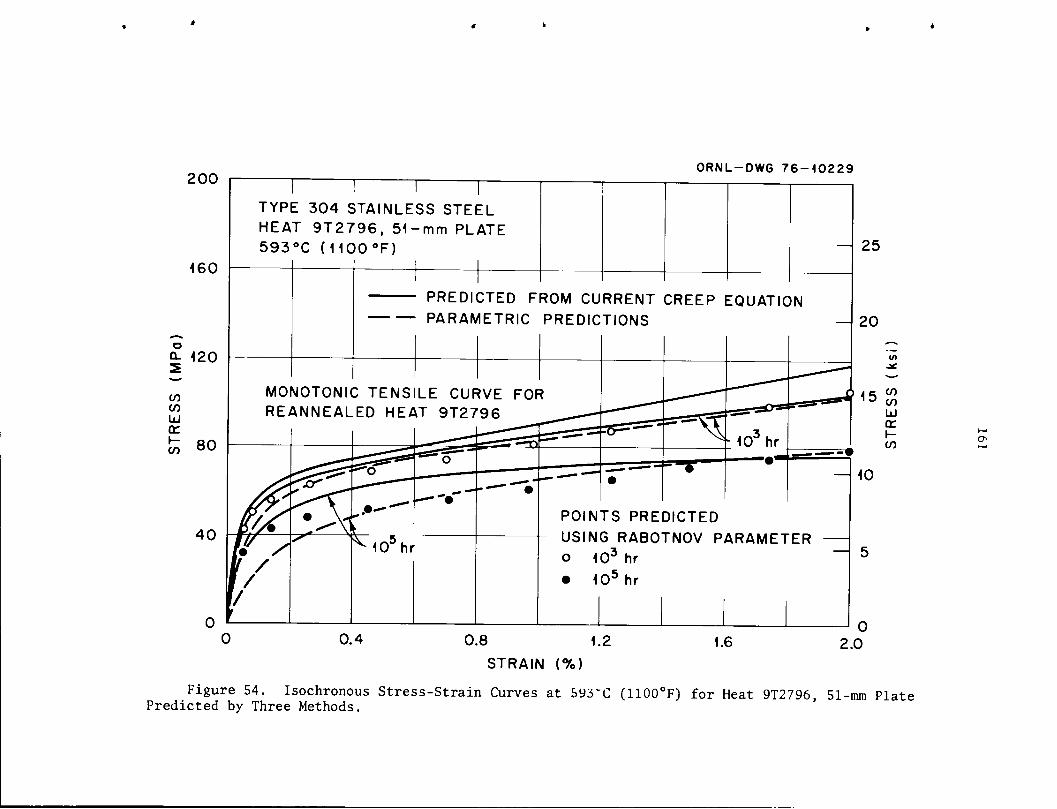
200
160
TYPE 304 STAINLESS STEEL
HEAT 9T2796, 51-mm PLATE593°C (1100°F)
ORNL-DWG 76-10229
25
PREDICTED FROM CURRENT CREEP EQUATIONPARAMETRIC PREDICTIONS
0.8 1.2
STRAIN (%)
2.0
Figure 54. Isochronous Stress-Strain Curves at 593"C (1100°F) for Heat 9T2796, 51-mm PlatePredicted by Three Methods.
o

162
1. time < the time to the onset of tertiary creep;
2. temperature in the range 427oC(800°F)-704oC(1300°F);
3. ultimate tensile strength within 42.8 MPa of the average
strength at temperature defined by Eqn. 22 on page 72.
Figure 46a, page 144, shows that the parameter C exhibits a maximum with
stress; the stress at the maximum (a ) is smaller for weaker heats or at
higher temperatures. This behavior is consistent with previous results
for both type 304 [27] and 316 [78,84] stainless steels. To avoid any
possible analytical difficulties, the value of ac can be taken as the
maximum applicable stress. Table XXXII gives the values of a^ at
various temperatures. The ranges shown are for minimum (lower values)
to maximum strength material in terms of ultimate tensile strength, with
the value of a increasing with material strength. Otherwise, thec
ultimate tensile strength of agiven heat is the maximum applicable stress
for that heat. Equation 73, page 141, predicts em >e3 for values of
e > 55.36%/hr. However, this anomaly occurs at stresses higher thanm
those cited above and does not affect the stated limits. The creep
equation is analytically valid to zero stress as the lower limit.
"Analytical" validity unfortunately does not necessarily imply
physical validity. Implications of extrapolating the current equations
are given in the next chapter.
Advantages
The creep equation presented herein has several important advantages
for design applications. First, the rational polynomial equation from
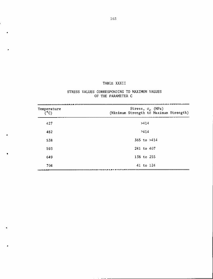
163
TABLE XXXII
STRESS VALUES CORRESPONDING TO MAXIMUM VALUES
OF THE PARAMETER C
Temperature Stress, ac (MPa)(°C) (Minimum Strength to Maximum Strength)
427 >414
482 >414
538 365 to >414
593 241 to 407
649 138 to 255
704 41 to 124

164
itself has distinct advantages over other popular forms. These
advantages were mentioned briefly above and are described in more detail
elsewhere [97].
The analysis of stress and temperature dependence used here clearly
alleviates the first objection to previous methods, since the results
depend largely upon rupture life and minimum creep rate data. Creep
curves are still needed, of course, to supply data for e , t , and e ,
and for verification of results. However, the current technique allows
utilization of all available information, rather than using available
creep curves only.
The empirical relationships [Eqns. 72-73, page 141, and 77, page 142,
used in developing the current equation are simpleand describe well the
experimental data. Therefore, fewer data are required to evaluate these
relationships than to develop direct expression for the parameters C and
p as functions of stress and temperature. The fact that the
relationships appear to closely reflect trends in the data lessens the
chance of obtaining misleading results, especially in the extrapolated
region, and avoids Objection 2.
The method used here inherently involves interrelationships among
the various equation parameters. Thus, the third objection is
eliminated.
Perhaps the most unusual and potentially useful feature of the
current equation is its ability to account for heat-to-heat variations,
alleviating Objection 4. It is not possible to predict the behavior
of every individual heat precisely. Still, an ability to reflect the

165
variation in strength from heat-to-heat can greatly decrease the
uncertainty involved in modeling elevated temperature mechanical
behavior. At the very least, the current approach gives a clear idea
of minimum and maximum strength, indicating the expected range of
behavior.
The method presented here is extremely flexible, and many
variations are possible. For instance t? may be modeled directly, as
were rupture life and minimum creep rate. Various methods for
predicting eg, including that used here, are presented in Ref. [51].
For instance, in some cases it may be possible to approximate eg by the
plasticity resource, e t . In that case, there would be even lessr J m r
reliance on actual creep curves than in the approach given here. An
alternate method for predicting heat-to-heat variations might be to
model t and e for given individual heats, which are known beforehandr m 6
to be strong, weak, medium, etc.
It is recognized that the current method also has some
disadvantages. These are primarily (1) that the predictions are
largely indirect, and (2) that the data bases used in different steps
may be different, yielding possible inconsistencies. The second problem
could easily be solved by using data from the same tests in every step,
but this approach limits the analysis to those tests for which all data
are available. The empirical relationships used are really
normalization procedures, so any inconsistencies should be small. In
short, we feel that the great advantages of the current approach far
outweigh any disadvantages.


CHAPTER V
EXTRAPOLATION OF RESULTS
An unavoidable problem incurred in the development of creep models
for design applications is the necessity to extrapolate results to
regions of time, stress, and perhaps temperature beyond the range of
experimental data. For example, a typical power plant operating life
is of the order of 300,000 hours (about 30 years), whereas the longest
experimental rupture life available in this investigation was 65,000
hours. Operating stresses and temperatures are chosen such that the
actual rupture life would be longer than the plant service life in
order to prevent component failures. Two specific examples illustrate
this situation.
First, a common problem in elevated temperature components is that
of "creep-fatigue," or cyclic deformation interspersed with periods of
monotonic creep or relaxation. Elevated temperature design rules [49]
specify a life fraction approach to the prevention of creep-fatigue
failures, based on the analysis proposed by Campbell [103]. This method
suggests that creep-fatigue failure be prevented by specifying that
P Q
I (n/JO, + I(^H < D* ' (83)j=l J k=l a K
where
D* = a specified "damage factor,"
167

168
n = the number of cycles applied under loading condition j,
Nn = the number of design allowable cycles under loading
condition j,
t = time duration of loading condition k,
Tn = allowable time under loading condition k.
T is calculated as the lower limit time to rupture at the temperature
of interest under a stress given by the stress from load k divided by
a factor K", which is defined as 0.9 for type 304 and 316 austenitic
stainless steels and for Incoloy Alloy 800H.
Since the quantity T is a lower limit estimate of rupture life,
design conditions are generally such that the evaluation of Eqn. 837 8
requires predictions of rupture lives to perhaps 10 or 10 hrs.
Second, a creep strain-time formulation is used to estimate the
magnitude of time-dependent (i.e. creep and relaxation) deformation
incurred in components during service. For example, it is expected
[104] that type 304 stainless steel will be used extensively as a
structural material in the reactor vessels and the intermediate heat
exchanger pressure boundaries for the Liquid Metal Fast Breeder
Reactor (LMFBR)[105]. Design conditions vary with the particular
application, but the maximum expected operating temperature for this
material in LMFBR service will be about 538°C (1000°F)[104]. In such
an application, the stresses on the material will be somewhere below
the allowable stress levels given in ASME Code Case 1592 [49].
Figure 55 compares this limited region of stress-temperature operating
conditions (for an operating life of 3x IO5 hours) with the region of

169
450
400
350
_ 30°oa.
5 250totoUJ
or 200
to
150
100
50
ORNL-DWG 77-3155
ALLOWABLE DESIGN 1CONDITIONS FOR IO5 hi
I (CODE CASE 1592)_l I
T
TYPE 304 STAINLESS STEEL
I INDICATES RANGE OF AVAILABLECREEP DATA
60
50
40 -
30 £
20
400 450 500 550 600 650
TEMPERATURE (°C)
700 750 800
Figure 55. Comparison of Stress-Temperature Operating ConditionsAllowed by ASME Code Case 1592 With the Range of Available ExperimentalCreep Data for Type 304 Stainless Steel.

170
the experimental creep tests used in the current evaluation. Estimation
of behavior for these operating conditions again can require
extrapolation to regions of stress and temperature well outside those
available experimentally.
A large number of data for type 304 stainless steel are available
over a large range of stress-temperature conditions. The material
appears well-behaved in this range, and its behavior can be adequately
described by simple empirical models. The problem with extrapolating
the results beyond the range of the data has two facets. First, there
is the possibility of long-term metallurgical instabilities such as
the formation of embrittling phases. Second, there is the possibility
that deformation and fracture mechanisms may be different in the
extrapolated stress-temperature region than in the region where data were
available. Otherwise, the amount of available data is sufficient to
warrant considerable extrapolation, and all of the models proposed
herein behave well analytically when extrapolated. Thus, it is
desirable to consider these two possibilities in more detail.
While there have been some indications [106] of sigma-phase
formation in long-term tests on type 304 stainless steel, available
data indicate that metallurgical stability is not a significant problem
for most practical applications [1]. The only change in fracture mode
appears to be the transition from transgranular to intergranular
fracture which occurs at short rupture times. Since most data reflect
this latter intergranular fracture mode, no problems should be incurred
in this respect as far as extrapolation is concerned.

171
The remaining uncertainty in extrapolating the current equations
beyond the range of data concerns possible changes in deformation
mechanism. A few low stress-low temperature tests which are still in
progress at ORNL indicate that such changes may occur. A detailed
fundamental investigation of creep deformation mechanisms is beyond the
scope of this report; however implications of mechanism changes on
predictive equations will be considered in the next section.
Possible Effects of Changesin Deformation Mechanism
Creep deformation can occur by a variety of mechanisms within the
same material at different stresses and temperatures. A convenient form
for presenting the deformation mechanisms that occur for a given
material is through the use of "deformation maps," recently devised by
Ashby [107,108]. These maps are plots on axes of stress versus
temperature, which show the areas in cr-T space where different creep
mechanisms are dominant. (Actually Frost and Ashby plotted normalized
shear stress a /u vs T/T where u is the shear modulus and T the melting
temperature. This choice was mainly to reduce variations among
materials and is not mandatory.)
Due to the many approximations and simplifications used by Frost
and Ashby in constructing their maps, the maps probably cannot be used
for quantitative design calculations. Nevertheless, the construction
contains useful qualitative information that can be helpful in defining
possible areas of uncertainty in predictions and in identifying areas
where more data are needed.

172
At high stress values, the dominant creep mechanism should involve
flow by dislocation glide. These stresses are higher than most of
those seen in the current data and are certainly higher than those of
interest in design applications. Therefore, this mode of deformation
will not be discussed here.
Virtually all of the currently available creep data fall in the
region where deformation is expected to be controlled by dislocation
creep (with the possible exception of a few of the ORNL low stress
creep tests that are still in progress). Creep in this region occurs
primarily through the motion of dislocations by both glide and climb.
Theoretical considerations [109] dictate that the steady-state creep
rate in this region should be given by
e -AD g-m v kT G
V. J
(84)
where A and n are material constants (n % 4), G is the shear modulus,
b is the burgers vector and k is Boltzmann's constant. Dy is the bulk-O/RT
diffusion coefficient, given by D = D e v/ . Equation 84 suggests
that a log e — log a plot should be linear, which is born out by the
current results. However, the current data show a slope of this
curve which decreases with temperature but is considerably larger than
4; also the observed activation energy appears to be somewhat larger
than that for vacancy self-diffusion in this material. Both of these
observations are common for creep-resistant engineering alloys. Many
investigators, for example Refs. [94,110-116], have attributed these
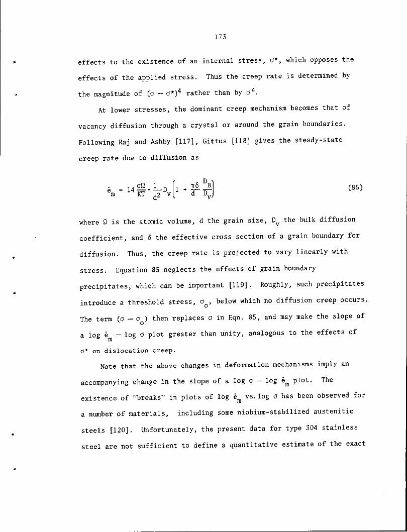
173
effects to the existence of an internal stress, o*, which opposes the
effects of the applied stress. Thus the creep rate is determined by
the magnitude of (a - a*)4 rather than by a4.
At lower stresses, the dominant creep mechanism becomes that of
vacancy diffusion through a crystal or around the grain boundaries.
Following Raj and Ashby [117], Gittus [118] gives the steady-state
creep rate due to diffusion as
r D 'ail 1 „ L HfLJl
d Dv-
e = 14 iiH • —Dem KT d2 v(85)
where ft is the atomic volume, d the grain size, Dy the bulk diffusion
coefficient, and 6 the effective cross section of a grain boundary for
diffusion. Thus, the creep rate is projected to vary linearly with
stress. Equation 85 neglects the effects of grain boundary
precipitates, which can be important [119]. Roughly, such precipitates
introduce a threshold stress, a , below which no diffusion creep occurs.
The term io - o ) then replaces a in Eqn. 85, and may make the slope of
a log e - log a plot greater than unity, analogous to the effects of
a* on dislocation creep.
Note that the above changes in deformation mechanisms imply an
accompanying change in the slope of a log a - log em plot. The
existence of "breaks" in plots of log em vs.log a has been observed for
a number of materials, including some niobium-stabilized austenitic
steels [120]. Unfortunately, the present data for type 304 stainless
steel are not sufficient to define a quantitative estimate of the exact

174
point where the break occurs, or of the sharpness of the break. The
data merely indicate the possible existence of such a break. The current
minimum creep rate model (and thus the creep equation) will significantly
overestimate the creep strength of this material in the low stress region
if such a break does occur. Thus, it is important to consider the
possible implications of such a change in slope even though a detailed
quantitative analysis awaits additional data.
One cause of such breaks could be the occurrence of a metallurgical
instability, but this explanation does not appear likely in the case of
type 304 stainless steel. Thus, a change in deformation mechanism
appears to be a likely cause.
Figure 56 displays the minimum creep rate data from ORNL for heat
9T2796, estimated through fits of the rational polynomial creep equation
by the method of Bunatyan [100]. Many of these tests are still in
progress, and the values of e in Figure 56 are approximate (thus the
large amount of scatter). At low stresses, there appears to be a
possible break in the plots of log e vs. log a indicating a decrease in
the value of n (the slope of these curves). In Figure 56, the slope
below the break has arbitrarily been chosen as 4, but appears to be
consistent with the data.
The data do not permit a detailed analysis of the break in
Figure 56. However, two possible explanations can be given. First,
the break may indicate a transition from dislocation creep to diffusion
creep. The slope of 4 is perhaps too high for diffusion creep, although
this inconsistency may merely indicate that the transition is not yet
complete.

COtoUJor
co 10
ORNL-DWG 77-3156
TTTTT I I IMIIII I I Mill i i nun 11 iiiiii i iinni i i i iiiiii i i i iiiiii i i iinni i i i mm 10'TYPE 304 STAINLESS STEEL
HEAT 9T2796
INES REPRESENT
ISUAL BEST FITSDATA ESTIMATED FROM FITS OF RATIONAL
POLYNOMIAL CREEP EQUATION
1 11 HI I I IMIIII I I I IIIIII I I I IIIIII I I I IIIIII I I I IIIIII L
-10 10" IO-1 10" 10" 10" 10" 10"-2
10
em, MINIMUM CREEP RATE (%/hr)
REPRESENT
ENTAL DATA
427°C (800°F)482°C (900°F)538 °C (1000°F)593°C (HOOT)649°C (1200°F)704°C(I300°F)i i i urn i i I il
10"
10L
\or
COCOLU i—'
or ~j1- Cn
Figure 56. Minimum Creep Rate Data for Heat 9T2796 51-mm Plate of Type 304 Stainless Steel.Data shown include estimated values for low stress tests currently in progress. The data indicatea possible downward break in the log e — log a isothermals at low stresses.
m

176
A second explanation is that of Lagneborg and Bergman [116], who
based the following analysis of such breaks on the internal stress.
Their analysis was strictly applicable to classical precipitation-
hardened alloys, where a uniform dispersion of particles is precipitated
within the matrix. The case of an austenitic stainless steel, where
precipitation occurs preferentially on dislocations and at grain
boundaries, is more complicated, but analogies can be drawn. According
to Lagneborg and Bergman, the stress dependence of the creep rate
should be proportional to (a - a )4, where a is the internal stress
due to the resistance to dislocation motion caused by the precipitates
within the matrix. Above the break point, a is a constant whose value
strongly depends upon the size, shape, and spacing of the precipitate
particles. In this region, dislocations move past the particles either
by cutting through them or by the Orowan mechanism. The net effect is
to make the slope of a log a vs. log e plot somewhat larger than 4.
Below the break, Lagneborg and Bergman propose that dislocations surmount
the particles by a climb mechanism. In this region, they predict that
a should be proportional to a. Thus, the creep rate is proportional to
(a — Ka)4 = (1 - K) a ,again yielding a slope of 4 in a log a- log em
plot. Incidentally, a in this region is almost independent of the
size, shape, and spacing of the precipitate particles. Available data
do not permit a clear identification of the cause of the breaks shown
in Figure 56, and the fact that the slope below the break has been drawn
as 4 in that figure does not indicate a preference for the
Lagneborg-Bergman explanation on the part of the author. If the

177
Lagneborg-Bergman explanation is correct, another break may occur at
still lower stresses indicating a change to diffusional creep.
There is sound physical basis for believing that the break shown in
Figure 56, page 175, might be real. Consideration of a numerical
example points out the importance of a further study of these slope
changes. First, assume that the break is drawn in the proper place in
Figure 56. Now choose a possible design condition for temperature and
stress, say 593°C (1100°F) and 20 MPa (2.9 Ksi). The current analysis
of minimum creep rate data Eqn. 36, page 90, yields (for heat 9T2796)
an estimated value of e = 5.7 x io"11 %/hr. Assuming a slope of 4_7
below the break in Figure 56 yields a value of e = 3 x 10 %/hr.m
Assuming that the break is due to a change to diffusion creep and taking
the slope below the break to be 2 requires a slight alteration of the
placement of the break point in Figure 56 to remain as consistent as
possible with the data. This reconstruction yielded a value of
e =10 %/hr. Thus, such breaks can cause underestimates of the valuem
of e by Eqn. 36 by a factor of over 10 ! (On the other hand, the
net deviation in 10 hr would only be perhaps 0.1% strain.)
A second point that can be noted from Figure 56 is the decreased
temperature dependence of the minimum creep rate at lower temperatures
(< 538°C). This decrease could have several causes. First, at these
temperatures there appear to be very few carbides precipitated within
the grains or at the grain boundaries. Thus, the strengthening effect
of these particles is lost at these low temperatures. A second possible
cause involves the often observed phenomenon, e.g. Ref. [121], of a
lower activation energy for creep at lower temperatures. Robinson and
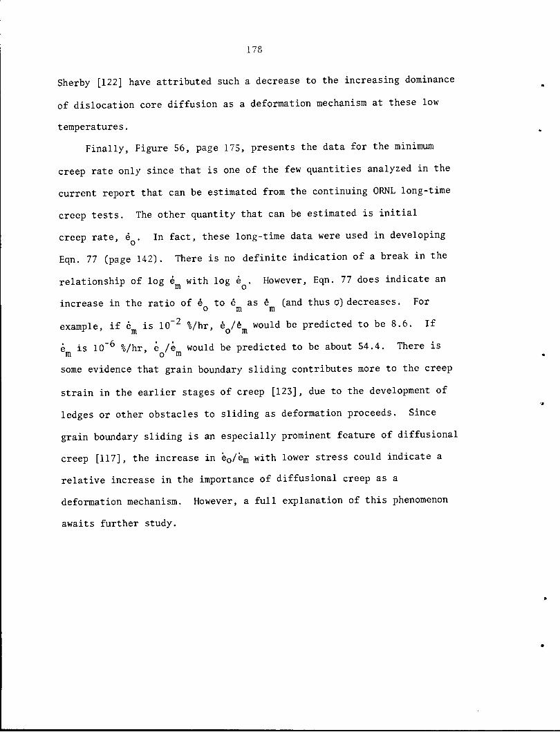
178
Sherby [122] have attributed such a decrease to the increasing dominance
of dislocation core diffusion as a deformation mechanism at these low
temperatures.
Finally, Figure 56, page 175, presents the data for the minimum
creep rate only since that is one of the few quantities analyzed in the
current report that can be estimated from the continuing ORNL long-time
creep tests. The other quantity that can be estimated is initial
creep rate, e . In fact, these long-time data were used in developing
Eqn. 77 (page 142). There is no definite indication of a break in the
relationship of log e with log e . However, Eqn. 77 does indicate an
increase in the ratio of e to e as e (and thus a) decreases. Foro m m
example, if e is IO"2 %/hr, eQ/em would be predicted to be 8.6. If
e is IO"6 %/hr, e /e would be predicted to be about 54.4. There ism ' o m r
some evidence that grain boundary sliding contributes more to the creep
strain in the earlier stages of creep [123], due to the development of
ledges or other obstacles to sliding as deformation proceeds. Since
grain boundary sliding is an especially prominent feature of diffusional
creep [117], the increase in e0/em with lower stress could indicate a
relative increase in the importance of diffusional creep as a
deformation mechanism. However, a full explanation of this phenomenon
awaits further study.
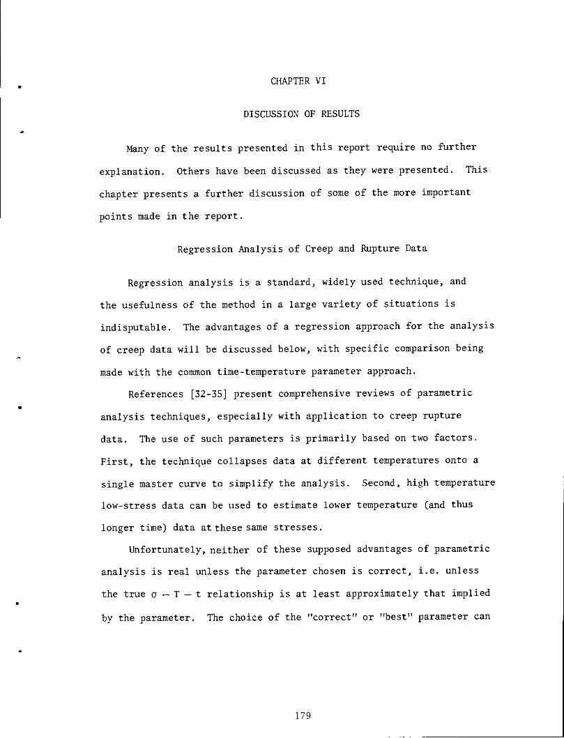
CHAPTER VI
DISCUSSION OF RESULTS
Many of the results presented in this report require no further
explanation. Others have been discussed as they were presented. This
chapter presents a further discussion of some of the more important
points made in the report.
Regression Analysis of Creep and Rupture Data
Regression analysis is a standard, widely used technique, and
the usefulness of the method in a large variety of situations is
indisputable. The advantages of a regression approach for the analysis
of creep data will be discussed below, with specific comparison being
made with the common time-temperature parameter approach.
References [32-35] present comprehensive reviews of parametric
analysis techniques, especially with application to creep rupture
data. The use of such parameters is primarily based on two factors.
First, the technique collapses data at different temperatures onto a
single master curve to simplify the analysis. Second, high temperature
low-stress data can be used to estimate lower temperature (and thus
longer time) data at these same stresses.
Unfortunately, neither of these supposed advantages of parametric
analysis is real unless the parameter chosen is correct, i.e. unless
the true a — T — t relationship is at least approximately that implied
by the parameter. The choice of the "correct" or "best" parameter can
179

180
be somewhat complicated. Dozens of distinct parameters have been
proposed. When the various possible stress dependences are considered,
the total number of parameters climbs into the hundreds.
It must be realized that even though a given parameter fits the
available data, that same parameter may not yield accurate
extrapolations. The last chapter indicated some of the problems that
can occur in the extrapolation of creep data. Parametric prediction of
low-stress, low-temperature data by higher temperature data at those
stresses represents an extrapolation and should only be done with
extreme caution. Figure 57 illustrates this situation schematically.
Thus, even though a point may lie within the range of the "master
curve," it can still represent an extrapolation and should be treated
accordingly.
Another problem incurred with time-temperature parameters is their
lack of flexibility. Larke and Inglis [124] presented an analysis of
the restrictions imposed by various commonly used parameters. Also,
variables other than stress and temperature may be important (such as
ultimate tensile strength). Within the form of a given parameter, the
flexibility with which new variables can be added is severely restricted.
Finally, it is often difficult to estimate the constants in the
parametric equations with accuracy except by the use of regression
techniques, especially for large multiple-heat data sets. Many of the
common parameter forms can be rewritten as linear regression models
with log e or log t as the dependent variable, although some becomem r
nonlinear models when written in this way. Thus, if one is essentially
reduced to using regression analysis anyway, it is a logical extension

181
ORNL-DWG 77-5109
A PARAMETRIC MASTER CURVE INCLUDES REGIONSTHAT ARE EXTRAPOLATED BEYOND THE RANGE OFEXPERIMENTAL DATA.
crz>
<tr
o.
LUI-
\<—AVAILABLE RANGE —•!
STRESS
Figure 57. Schematic Illustration of the Region of InterpolationVersus Extrapolation for Creep Data. Any point within the boxed regionlies within the parametric "master curve," while only points within theshaded region lie within the range of experimental data.

182
to consider a generalized set of models rather than restricting the
analysis to a small subset which also happen to correspond to
time-temperature parameters. Regression will in general yield a single
well-behaved mathematical model with clear statistical implications.
Thus, such a technique is particularly useful for analyses whose results
are intended for design applications.
Once regression analysis has been selected as the technique to use,
a variety of options still remain. In particular, the final "optimum"
model can be selected by a number of techniques. In the case of creep
data, the method used here has the advantage that several candidate
models are output from the statistical selection procedure so that some
physical judgment can be applied in the choice of a final model. If one
merely wishes to represent a set of data and is not interested in
extrapolation, it would be sufficient to use a procedure (such as
stepwise regression) which might yield only one optimum model based
solely on statistical considerations.
No representation is made that the current technique is the best
possible. This technique is, however, very useful and easily applied.
It allows considerably more flexibility than a parametric analysis, and
the results are easily applied to design. Perhaps the most controversial
aspect of the particular results given here is the use of ultimate
tensile strength as an indicator of heat-to-heat variations in creep
strength.

183
Relationship Between Ultimate Tensile Strengthand Creep Properties
One of the more powerful features of the current formulation is
the ability to predict heat-to-heat variations in creep behavior from
a knowledge of the ultimate tensile strength of a given heat of material.
The models presented herein also embody a much sought after relationship
between short-term tensile properties and long-term creep properties.
Therefore, it is desirable to examine the validity of this relationship
in more detail.
The use of U to aid in predicting creep behavior is not a totally
novel approach. For instance, Conrad [125] proposed an equation of the
form
tr =Dexp ffl exP aQ(T) (86)
where D is a constant, H the activation energy of self-diffusion, R the
gas constant, and a is some measure of variation of strength with
temperature. Our use of ultimate tensile strength is a similar concept.
Various American [126-129] and Soviet [130-132] investigators have
related either hot-hardness or ultimate tensile strength at temperature
to creep and creep rupture strength. These investigations are summarized
in Ref. [20].
Analytically, the ultimate tensile strength, U, can be considered
as the stress corresponding to a rupture life of the duration of a
tensile test or to a minimum creep rate of the tensile strain rate.

184
Therefore, the ultimate tensile strength for a given heat of material at
a given temperature effectively determines the location of the short
time/high rate end of the stress-rupture or stress-minimum creep rate
isotherm for that heat at that temperature.
Sikka et al. [20] have discussed the metallurgical factors involved
in relating ultimate tensile strength to creep behavior. For
completeness, their arguments will be reproduced here. Perhaps the
main objection to the use of ultimate tensile strength to predict creep
behavior is the possibility that metallurgical changes which occur
during long-term creep may sufficiently alter material behavior so as to
destroy any correlation between ultimate tensile strength and long-term
creep or creep rupture strength. For type 304 stainless steel, the
metallurgical changes are limited primarily to precipitation of carbides
at grain boundaries and in the matrix. ORNL data for test times
approaching 40,000 hr show the weak or strong character of a heat to be
retained during a long-term test, which indicates that metallurgical
changes have comparatively little influence on factors controlling the
relative creep strength of various heats. There is evidence [1] that
thermal aging for a period of 100,000 hr (11.4 yr) at 565°C (1050°F)
causes essentially no changes in the creep properties of type 304
stainless steel. The apparent linearity in log a vs. log tr and
loe a vs. log e isotherms for the current data extends to test times& ° m
of 65,000 hr, indicating thereby the absence of any significant
metallurgical changes in this period of time [133].
Another question which should be addressed concerns possible
effects of differences between creep and tensile modes of deformation.
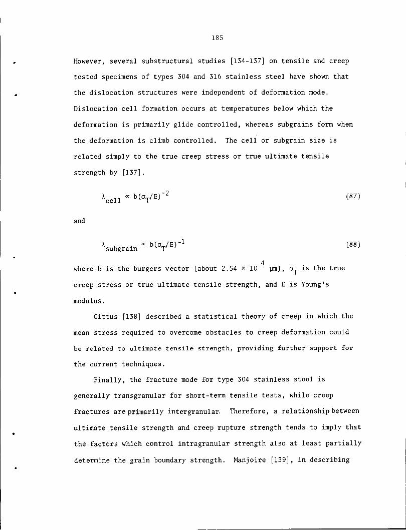
185
However, several substructural studies [134-137] on tensile and creep
tested specimens of types 304 and 316 stainless steel have shown that
the dislocation structures were independent of deformation mode.
Dislocation cell formation occurs at temperatures below which the
deformation is primarily glide controlled, whereas subgrains form when
the deformation is climb controlled. The cell or subgrain size is
related simply to the true creep stress or true ultimate tensile
strength by [137] .
Acell * MaT/E)-2 (87)
and
a , . « biojE)-1 (88)subgrain v T
-4where b is the burgers vector (about 2.54 x 10 um), a„ is the true
creep stress or true ultimate tensile strength, and E is Young's
modulus.
Gittus [138] described a statistical theory of creep in which the
mean stress required to overcome obstacles to creep deformation could
be related to ultimate tensile strength, providing further support for
the current techniques.
Finally, the fracture mode for type 304 stainless steel is
generally transgranular for short-term tensile tests, while creep
fractures are primarily intergranular. Therefore, a relationship between
ultimate tensile strength and creep rupture strength tends to imply that
the factors which control intragranular strength also at least partially
determine the grain boundary strength. Manjoire [139], in describing

186
flow and fracture, suggested that the same factors influence the
relative strengths of both the grain matrix and the grain boundary.
There is much evidence that grain boundary sliding and intragranular
deformation during creep are related [139]. Additional support for this
contention can be found in the work of Rhines and Wray [140] and Sikka
et al . [141], who have studied the minima in tensile ductility
with temperature exhibited by austenitic stainless steels. Figure 58
shows the tensile reduction of area as a function of test temperature
for the weakest and strongest (in terms of ultimate tensile strength)
heats in the ORNL testing program for types 304 and 316 stainless steel.
As noted in Ref. [141], the weak heats show a drop in ductility at
temperatures which are in the creep range. Rhines and Wray [140]
offered an explanation for such ductility minima. At the lower
temperatures, failure occurs by a transgranular crack propagation
mechanism, and ductility is high. As temperatures approach the
temperature of the minimum in ductility, some deformation occurs by
grain-boundary shear, resulting in rapid growth of intergranular voids
formed at triple points, causing a drastic loss in ductility. As the
temperatures become still higher, recrystallization occurs along with
the intergranular void formation, continuously breaking up the
intergranular fracture path and causing the ductility to again increase.
Figure 58 indicates that the ductility minimum associated with
intergranular cracking occurs in the weak heat of type 304, but is
either absent or postponed to higher temperatures in the strong heat.
This effect can be explained in terms of the increased grain boundary
strength of these strong heats. Since these same heats have high

100
90
80
70
60
O 50
oZ>QLU
tr
40
9•V
\\
\•
— --
\
»__
••
N'^.
\
~~ GRAI N SIZE STF(ENGTH
(^.m) TENSILE AND CREEP HEAT NO.
o 230 WEAK 796 K
— • 78 STRONG 813
€ = 0.004/min
1YPt 304, RtANNEALED
PRESENT INVESTIGATION
(<7>
30 —
ORNL-DWG 76-79H
3/
•
II
1I
^*5Q
^^^^ A •
/
"^\*>i
•
\ 7°1 A
•
\ !\ /\ /
//
//
\V!C
CONDITION GRAIN SIZE e/min
— • AS-RECEIVED ASTM 5-7 0.0018 -
o AS-RECEIVED ASTM 5-3 (50/im) 0.0040a REANNEALED ASTM 3-6 (90^m) 0.0040
STRENGTH
TENSILE AND CREEP REFERENCE
• STRONG STEICHEN
o M/FRflPF PRESENTAVtKAbt INVESTIGATION (PI)
a AVERAGE PI
TYPE 316
(b)
20
10
200 400 600
TEST TEMPERATURE (°C)
800 0 200 400 600
TEST TEMPERATURE CO
800
Figure 58. Trends in the Tensile Reduction of Area With Temperature for Weak and Strong Heatsof Types 304 and 316 Stainless Steel.
oo

188
values of U, their matrix strength is also relatively high. These
observations support the proposition that inter- and intragranular
strengths are related and are perhaps controlled by similar factors.
The use of ultimate tensile strength in predicting creep and
creep-rupture strength for type 304 stainless steel is justified both
by an empirical, statistically based modeling procedure and by more
fundamental metallurgical considerations. An alternative might be to
use some direct measure of the property being modeled as an indicator
of the strength of a given heat. For instance, the stress to cause
2rupture in 10 hours at the temperature of interest or the stress to
-2cause a minimum creep rate of 10 %/hr might be used as variables
rather than ultimate tensile strength. However, the use of ultimate
tensile strength appears adequate and is easier to apply.
Predicted Trends in Ductility Data
Although these analyses were done primarily on an empirical
basis, the results appear consistent with those that would be expected
from a physical model. The predictions of the variations in creep
ductility in Chapter III illustrate this point. It is generally accepted
that the observed creep strain consists of the strain occurring within
individual grains (e ) and the deformation occurring by grain boundary
sliding (e,). Thus,
e3 = eg + eb ' (89)
where the values of e and e, depend on the relative strengths of grain

189
matrix and grain boundaries. Since the annealing treatment in the type
304 stainless steel does not cause the formation of strengthening
phases, applied creep stress can produce deformation both in the matrix
and at grain boundaries. The matrix deformation causes the formation of
a subgrain or dislocation cell structure; meanwhile, the grain boundary
deformation causes stress concentrations. For test temperatures below
about 649°C, carbide precipitates deposited at the grain boundaries
during testing are continuous and thus inhibit [142] both grain boundary
sliding and migration. As a result, the stress concentrations generated
at triple points can nucleate cracks [143] causing onset of tertiary
creep after only small strains at low temperatures. Precipitates at
higher temperatures are larger and make possible both grain boundary
sliding and migration. Grain boundary migration can relax stresses,
thus allowing a greater intergranular deformation before the initiation
of enough cracks to cause onset of tertiary creep. There is a great
deal of evidence that an increase in stress results in a decrease of
the contribution of grain boundary sliding to the total strain [123].
Thus, the amount of matrix deformation incurred before the occurrence
of intergranular cracks increases as stress increases. The effect of
strain rate is similar. Equation 40, page 103, predicts a decrease in
the ratio of t, or t within increasing time (decreasing strain rate),
due to the larger contribution of grain boundary deformation and
faster cracking under these conditions.
The predicted variations in creep ductility due to ultimate tensile
strength can also be explained. A given applied stress is effectively
lower for a strong heat than for a weak heat. Thus, the isostress

190
effect of increasing strength (U) is similar to the effect of decreasing
stress, i.e., a decrease in ductility. However, at very high stresses,
the increased strength of strong heats begins to dominate and stronger
heats can withstand more deformation before cracking and the onset of
tertiary creep. At a constant strain rate, the increased grain boundary
strength of stronger heats results in an increased contribution of
intragranular deformation to the total strain. Therefore, more strain
occurs before grain boundary deformation is sufficient to cause
extensive cracking and the onset of tertiary creep. At a constant
strain rate, 63 is thus generally larger for stronger heats. In
short, all of the trends predicted by the current empirical calculations
are consistent with the metallurgical features of this material.
Comparison With ASME Code Case 1592Allowable Stress Levels
The current results can be directly compared with the results
given in ASME Code Case 1592 [49] in terms of the time dependent
allowable stress levels, S , for elevated temperature applications.
The value of S is defined as the lowest of the three following
criteria:
1. 2/3 of S , the minimum stress to cause rupture in time t;
2. 80% of S3, the minimum stress to cause onset of tertiary
creep in time t;
3. Sl0, the minimum stress to cause 1% total strain in time t.1 ~h
Values of S and S are tabulated directly in ASME Code Case 1592
[49]. For the current results S , S7, S,0, and S^ were calculated atL J r 3 1%' t
191
3 5times of 10 hours and 10 hours. Values of S,<^ were taken directly
from the minimum strength isochronous stress-strain curves from
Figure 53, pages 156-158). Values of S were determined using Eqn. 35,
page 88, and evaluating at minimum values ofultimate tensile strength
(mean minus two standard errors). Values of S3 were calculated
similarly, using Eqn. 40, page 103, to estimate t from t •
Table XXXIII compares the current results with those of the code
case. Considering the large differences in data bases and analytical
techniques, the two sets of values correspond quite closely. The
current minimum values are in general slightly lower than those of the
code case, perhaps reflecting the large variations in strength displayed
by the current ORNL data. As explained above, many uncertainties
remain in the extrapolated regions. The current results do not in
themselves indicate any alarming problems in the results of ASME Code
Case 1592 [49].
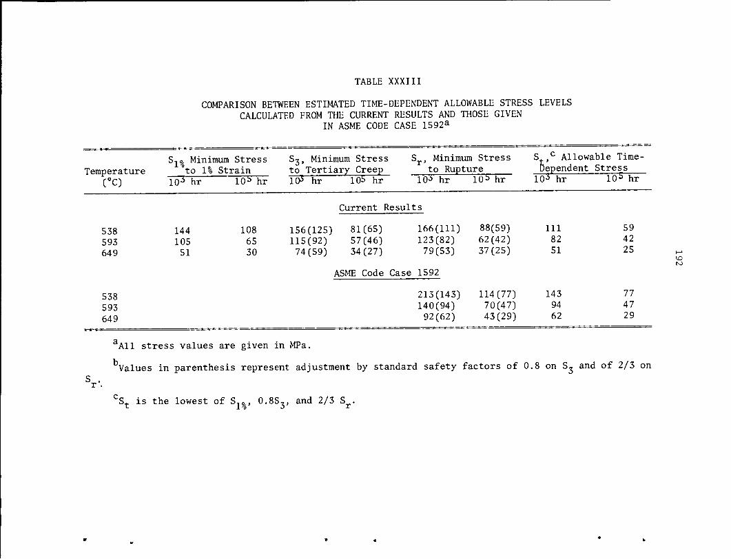
TABLE XXXIII
COMPARISON BETWEEN ESTIMATED TIME-DEPENDENT ALLOWABLE STRESS LEVELSCALCULATED FROM THE CURRENT RESULTS AND THOSE GIVEN
IN ASME CODE CASE 1592a
Temperature
Sl9. Minimum Stress"to 1% Strain
S3, Minimum Stress Sr, Minimum Stressto Tertiary Creep to Rupture
S c AllowableDependent Stre
10-* hr 10
Time-
ss
5 hr(°C) 10-* hr IO15 hr 10s hr 10S hr 10-* hr 103 hr
Current Results
538
593
649
144
105
51
108
65
30
156(125) 81(65) 166(111)115(92) 57(46) 123(82)74(59) 34(27) 79(53)
ASME Code Case 1592
88(59)62(42)37(25)
111
82
51
59
42
25
538
593
649
213(143)140(94)92(62)
114(77)70(47)43(29)
143
94
62
77
47
29
S .r .
aAll stress values are given in MPa.
Values in parenthesis represent adjustment by standard safety factors of 0.8 on S^ and of 2/3 on
S+. is the lowest of S,0, 0.8S,, and 2/3 S .x. i *g o r
(Dro

CHAPTER VII
CONCLUSIONS
A large base of creep and creep-rupture data for type 304 austenitic
stainless steel has been subjected to an analytical treatment in order
to develop a mathematical representation of the properties of this
material for design applications. Specific conclusions of the current
analysis are:
1. Standard techniques of linear regression analysis can be
applied to develop analytical models for rupture life (t ) and minimum
creep rate (em). These models fit the data well, including the
prediction of heat-to-heat variations in properties through the
inclusion in the models of terms involving the ultimate tensile strength
of a given heat of material at the temperature of interest. However,
extrapolation of these models is only valid so long as no significant
metallurgical changes (instabilities or deformation mechanism changes)
occur. The final equations used were:
log tr =5.716 -^M- logo +1^U -0.007303 Ulog a (90)
log em =-2.765+^- log a--il^4" +0. 01616 Ulogo . (91)
2. The use of variations in ultimate tensile strength to estimate
variations in creep and rupture strength is consistent with available
data and appears to be reasonable based on metallurgical considerations.
193

194
3. Simple empirical relationships can be used to estimate the
time to tertiary creep, t3, from the time to rupture. The average
creep rate to tertiary creep, e3 = e3/t3 (e3 is the creep strain at the
onset of tertiary creep), can be estimated from the minimum creep
rate. These relationships are:
t, = 0.686 t °"968 (92)3 r
and
e =1.11 em0-974. (93)3 m
Thus, the creep strain to tertiary creep, e3, can be estimated by
„ ,,., „ 0.968 . 0.974e3 = 0.761 tr 94)
Alternatively, e3 and t3 can each be separately modeled by regression
analysis and then multiplied to yield ey Other creep ductility criteria
(e.g., the strain to rupture) can be similarly estimated. Predicted
trends in creep ductility appear consistent with the metallurgical
characteristics of type 304 stainless steel.
4. Type 304 stainless steel generally exhibits classicial three
stage creep. The shape of the strain-time creep curves in the primary
and secondary stages can be adequately modeled by the single rational
polynomial creep equation,
e = CPt + et , (95)c 1 + pt m '

195
where e is the creep strain, t the time, and C, p, and e are equation
parameters (e = minimum creep rate).
5. The parameter C corresponds to the total amplitude of the
primary term in the rational polynomial creep equation. It can be
shown that C = t_(e_ — e ), so that the equations given in conclusion
(3) above yield
C = 0.686 t°-968(l.ll e0-974 -e ) . (96)r v m mJ K J
The initial creep rate, e = Cpte , can be estimated by
. 0.80e = 3.43 e , (97)o m ' v J
so that the parameter p can be estimated by
(e - e )
P =-2-^ • (98)
Thus, the entire creep equation can be estimated from a knowledge of
e and t alone. The above models (Eqns. 90 and 91,page 193) thus yield a
prediction of the strain-time behavior which reflects heat-to-heat
variations in creep strength through variations in ultimate tensile
strength. (Equations 92-94, 96, and 97 appear to be relatively
insensitive to heat-to-heat variations, since they are normalization
procedures.)
6. The occurrence of metallurgical instabilities 'does not appear
to be a significant problem for type 304 stainless steel. However,
available low-stress creep tests from Oak Ridge National Laboratory
(many of which are still in progress) appear to indicate a change in

196
deformation mechanism at low stresses. As a result, the above
equations would be valid only to the point where this change occurs.
The data do not permit an exact determination of the nature of this
change, but metallurgical considerations show that it is reasonable to
expect such a change. A quantitative analysis of behavior below the
break requires more data than are currently available. In particular,
there is no information about heat-to-heat variations in properties
below the break. The creep process appears to display a lower
activation energy at lower temperatures.
7. By using an estimated minimum value of ultimate tensile
strength in the predictive equations, the behavior of minimum strength
material can be estimated. These results can be compared with the
allowable stress levels for this material given in ASME Code Case 1592,

REFERENCES


REFERENCES
l W E Ray et al., "Selection of Steam Generator Tubing Material forthe Westinghouse LMFBR Demonstration Plant," Nuclear Technology,Vol. 11, June 1971, pp. 222-231.
7 R A Moen et al., "Specifying and Manufacturing Piping for the2- Fast'FluxVest Facility," Li f^t^^P^SW^Austenitic Stainless Steels, A. 0. scnaeier ed., The American
Society of Mechanical Engineers, New York, 1974, pp. 141-155.
3. R. Stickler and A. Vinckier, "Morphology of GrJi»:J°^"^fbideSand Its Influence on Intergranular Corrosion of 304 StainlessSteel," Transactions of the American Society for Metals_,Vol. 54, 1961, pp. 362-380.
4.B. Weiss and R. Stickler, "Phase Instabilities During HighTemperature Exposure of 316 Austenitic Stainless Steel,Metallurgical Transactions, Vol. 3, 1972, pp. 851-866.
5 J E Spruiell et al., "Microstructural Stability of Thermal-' Mechanically Pretreated Type 316 Stainless Steel," Met. Trans.,
Vol. 4, 1973, pp. 1533-1544.
6 C F Etienne, W. Dortland, and H. B. Zeedijk, "On the Capabilityof Austenitic Steel to Withstand Cyclic Deformation During Serviceat Elevated Temperature," paper presented at InternationalConference on Creep and Fatigue in Elevated TeyeratureApplications, Philadelphia, September l»i>, and Sheffield, UK,April 1974.
7. V. K. Sikka, C. R. Brinkman, and H. E. McCoy, Jr., "Effect ofThermal Aging on Tensile and Creep Properties of Types 304 andIl6 Stainlesf Steels," in Structural Materials for Service atElevated Temperatures in Nuclear Power Generation MPC-1A. 0 Schaefer, ed., American Society ot Mechanical Engineers,New York, 1975, pp. 316-350.
8. C. E. Pugh et al., Currently Recommended Constitutive Equationsfor Inelastic Design^nJlTsTs of FFTF Components, ORNL-TM-3602(September 1972).
9.J M. Corum et al., Interim Guidelines for Detailed InelasticAnalysis of High-Temperature Reactor System Components,ORNL-5014 (December 1974). ~~
199

200
10. C. E. Pugh et al., Background Information for Interim Methods ofInelastic Analysis for High-Temperature Reactor Components of2 1/4 Cr-1 Mo Steel, ORNL-TM-5226 (May 1976).
11. C. E. Pugh, "Constitutive Equations for Creep Analysis of LMFBRComponents," in Advances in Design for Elevated TemperatureEnvironment, S. Y. Zamrik and R. I. Jetter, eds., The AmericanSociety of Mechanical Engineers, New York, 1975, pp. 1-15.
12. C. C. Davenport, "Correlation of Creep and Relaxation Properties ofCopper," J. Appl. Mech., Vol. 60, 1938, p. A-55.
13. V. K. Sikka, H. E. McCoy, Jr., M. K. Booker, and C. R. Brinkman,"Heat-to-Heat Variations in Creep Properties of Types 304 and316 Stainless Steels," J. Pressure Vessel Technology, Vol. 93,No. 4, Nov. 1975, pp. 243-251.
14. Interpretations of the ASME Boiler and Pressure Vessel Code,Case 1592, American Society of Mechanical Engineers, New York,1974.
15. V. K. Sikka, R. W. Swindeman, C. R. Brinkman, and M. K. Booker,Residual Cold Work and Its Influence on Tensile and CreepProperties of Types 304 and 316 Stainless Steel, ORNL-TM-5192(January 1976), also published in Nuclear Technology, Vol. 31,Oct. 1976, pp. 96-114.
16. V. K. Sikka, T. L. Hebble, M. K. Booker, and C. R. Brinkman,Influence of Laboratory Annealing on Tensile Properties andTime-Independent Design Stress Intensity Limits for Type 304Stainless Steel, ORNL-5175 (December 1976).
17. V. K. Sikka, Oak Ridge National Laboratory, Private communication(June 1976).
18. V. K. Sikka and M. K. Booker, "Assessment of Tensile and CreepData for Types 304 and 316 Stainless Steels," presented atInternational Joint Pressure Vessels and Piping and PetroleumMechanical Engineering Conference, Mexico City, Mexico,September 19-24, 1976. To be published in Journal of PressureVessel Technology.
19. V. K. Sikka and C. R. Brinkman, "Relation Between Short- andLong-Term Elevated-Temperature Properties of SeveralStainless Steels," Scripta Met., Vol. 10, 1976, pp. 25-28.
20. V. K. Sikka and M. K. Booker, "Use of Ultimate Tensile Strength toCorrelate and Predict Creep and Creep Rupture Behavior of Types 304and 316 Stainless Steel," report in preparation.
21. BSCC High-Temperature Data, Published for the British SteelmakersCreep Committee by the Iron and Steel Institute, 1973.

201
22. "NRIM Creep Data Sheets: Elevated-Temperature MaterialsManufactured in Japan, 1973," National Research Institute forMetals, Tokyo 153, Japan.
23. W. F. Simmons and H. C. Cross, Report on the Elevated-TemperatureProperties of Stainless Steels, ASTM Special TechnicalPublication 124, American Society for Testing and Materials,Philadelphia, 1952.
24. W. F. Simmons and J. A. Van Echo, Report on the Elevated-TemperatureProperties of Stainless Steels, ASTM Data Series Publication DS5-S1,American Society for Testing and Materials, Philadelphia, 1955.
25. H. E. McCoy, Interim Report of Tensile and Creep Data for Type 304Stainless Steel Plate (Reference Heat 9T2796, 2 in. Thick),ORNL-TM-4627 (October 1974).
26. H. E. McCoy, Tensile and Creep Properties of Several Heats ofType 304 Stainless Steel, ORNL-TM-4709 (November 1974).
27. R. W. Swindeman and C. E. Pugh, Creep Studies on Type 304 StainlessSteel (Heat 8043813) Under Constant and Varying Loads, ORNL-TM-4427(June 1974).
28. R. W. Swindeman, "Creep-Rupture Correlations for Type 304 StainlessSteel Heat 9T2796," in Structural Materials for Service at ElevatedTemperatures in Nuclear Power Generation, MPC-1, A. 0. Schaefer,ed., American Society of Mechanical Engineers, New York, 1975,pp. 1-29.
29. L. D. Blackburn, "Isochronous Stress-Strain Curves for AusteniticStainless Steels," in The Generation of Isochronous Stress-StrainCurves, A. 0. Schaefer, ed., American Society of MechanicalEngineers, New York, 1972, pp. 15-48.
30. ASTM Designation: A 240-71, "Standard Specification for Stainlessand Heat-Resisting Chromium and Chromium-Nickel Steel Plate, Sheetand Strip for Fusion Welded Unfired Pressure Vessles," Annual Bookof ASTM Standards, Part 3, American Society for Testing andMaterials, Philadelphia (April 1972).
31. ASTM Designation: A 479-71, "Standard Specification for StainlessSteel and Heat-Resisting Steel Bars and Shapes for Use in Boilersand Other Pressure Vessels," Annual Book of ASTM Standards, Part 3,American Society for Testing and Materials, Philadelphia(April 1972).
32. J. B. Conway, Stress-Rupture Parameters: Origin, Calculation andUse, Gordon and Breach, New York, 1969.
33. S. S. Manson, "Time-Temperature Parameters—A Re-Evaluation and SomeNew Approaches," Time-Temperature Parameters for Creep-RuptureAnalysis, ASM Publication D8-100, American Society for Metals,Metals Park, Ohio, 1968, pp. 1-114.

202
34. H. P. Van Leeuwen, Predicting Material Behavior Under Load, Time,and Temperature Conditions, Report 513, North Atlantic Treatyorganization Advisory Group for Aerospace Research and Development(June 1965).
35. R. K. Penny and D. L. Marriott, Design for Creep, McGraw-Hill,London, 1971, pp. 192-238.
36. S. S. Manson, "Design Considerations for Long Life at ElevatedTemperatures," James Clayton Lecture Presented at JointInternational Conference on Creep, London, 1963. Inst. Mech.Eng. Proc, Vol. 178, No. 3A, 1963-64, pp. 1045-1071.
37. A. Mendelson and S. S. Manson, "The Extrapolation of Families ofCurves by Recurrence Relations, With Application to Creep RuptureData," Trans. ASME, J. Basic Eng., Vol. 82, 1960, pp. 839-847.
38. M. K. Booker, T. L. Hebble, D. 0. Hobson, and C. R. Brinkman,Mechanical Property Correlations for 2 1/4 Cr-1 Mo Steel in Supportof Nuclear Reactor Systems Design, ORNL-TM-5329 (June 1976). To bepublished in International Journal of Pressure Vessels and Piping.
39. D. R. Rummler, "Stress-Rupture Data Correlation-GeneralizedRegression Analysis, An Alternative to Parametric Methods," presentedat ASTM Symposium on Reproducibility and Accuracy of MechanicalTests, St. Louis, Missouri, May 5, 1976.
40. N. R. Draper and H. Smith, Applied Regression Analysis, John Wileyand Sons, New York (1966).
41. C. Daniel and F. S. Wood, Fitting Equations to Data, John Wiley andSons, New York (1971).
42. R. R. Hocking and R. N. Leslie, "Selection of the Best Subset inRegression Analysis, Technometrics, Vol. 9, 1967, pp. 531-540.
43. L. R. LaMotte and R. R. Hocking, "Computational Efficiency inthe Selection of Regression Variables," Technometrics, Vol. 12,1970, pp. 83-93.
44. M. K. Booker, Regression Analysis of Creep-Rupture Data: A PracticalApproach, report in preparation.
45. F. R. Larson and J. Miller, "A Time-Temperature Relationship forRupture and Creep Stresses," Trans. ASME, Vol. 74, 1952, pp. 765-771.
46. S. S. Manson and G, Succop, "Stress-Rupture Properties of Inconel 700and Correlation on the Basis of Several Time-Temperature Parameters,"Symposium on Metallic Materials for Service Above 1600°F, ASTM STP174, American Society for Testing and Materials, Philadelphia, 1956,pp. 40-4b.
203
47. R. L. Orr, 0. D. Sherby, and J. E. Dorn, "Correlation of RuptureData for Metals at Elevated Temperatures," Trans. ASM, Vol. 46,1954, pp. 113-128.
48. G. T. Leiberman and R. G. Miller, Jr., "Simultaneous ToleranceIntervals in Regression," Biometrika, Vol. 50, 1963, pp. 165-181.
49. Interpretations of the ASME Boiler and Pressure Vessel Code,Case 1592. American Society of Mechanical Engineers, New York,1974.
50. M. K. Booker, C. R. Brinkman, and V. K. Sikka, "Correlation andExtrapolation of Creep Ductility Data for Four Elevated-TemperatureStructural Materials," in Structural Materials for Service atElevated Temperatures in Nuclear Power Generation, A. 0. Schaefer,ed., American Society of Mechanical Engineers, New York, 1975,pp. 108-145.
51. M. K. Booker and V. K. Sikka, Predicting the Strain to TertiaryCreep for Elevated-Temperature Structural Materials, ORNL-TM-5403(July 1976).
52. M. K. Booker and V. K. Sikka, Empirical Relationships Among CreepProperties of Four Elevated-Temperature Structural Materials,0RNL-TM-5399 (June 1976).
53. G. V. Smith, Properties of Metals at Elevated Temperatures,McGraw-Hill, New York, 1950, p. 151.
54. R. M. Goldhoff, "A Method for Extrapolating Rupture Ductility,"Elevated Temperature Testing Problem Areas, ASTM STP 488, AmericanSociety for Testing and Materials, Philadelphia, 1971, pp. 82-94.
55. F. C. Monkman and N. J. Grant, "An Empirical Relationship BetweenRupture Life and Minimum Creep Rate in Creep-Rupture Tests,"Proc. ASTM, Vol. 56, 1956, pp. 593-605.
56. M. K. Booker and V. K. Sikka, "Interrelationships Between CreepLife Criteria for Four Nuclear Structural Materials," NuclearTechnology, Vol. 30, July 1976, pp. 52-64.
57. N. J. Grant and A. G. Bucklin, "On the Extrapolation of Short-TimeStress-Rupture Data," Trans. ASM, Vol. 42, 1950, pp. 720-751.
58. N. J. Grant, "Stress Rupture Testing," High Temperature Propertiesof Metals, American Society for Metals, Cleveland, 1951, pp. 41-72.
59. V. S. Ivanova, "Creep Ductility Criterion for Metals," ZavodskayaLaboratoria, Vol. 21, No. 2, 1955, pp. 212-216; Brutcher TranslationNo. 4210.

204
60. I. A. Oding and V. S. Ivanova, "Analysis and Application ofCertain Creep Criteria," Vestnik Mashinostroeniya, Vol. 35, No. 5,1955, pp. 62-66; Brutcher Translation No. 4211.
61. R. M. Goldhoff, "Some Observations on the Extrapolation ofHigh-Temperature Ferritic Steel Data," J. Basic Eng.. Vol. 82,No. 4, Dec. 1960, pp. 848-853.
62. P. W. Davies and B. Wilshire, "An Interpretation of the RelationshipBetween Creep and Fracture," Structural Processes in Creep, Ironand Steel Institute, London, 1961, pp. 34-43.
63. F. Garofalo, Fundamentals of Creep and Creep Rupture, Macmillan,New York, 1965, p. 204.
64. R. Viswanathan, "Strength and Ductility of 2 1/4 Cr-1 Mo Steels inCreep at Elevated Temperatures," Metals Technology, Vol. 1,June 1974, pp. 284-294.
65. I. S. Servi and N. J. Grant, "Creep and Stress Rupture Behaviorof Aluminum As a Function of Purity," Trans. AIME, Vol. 191,1951, pp. 909-916.
66. E. S. Machlin, "Creep-Rupture by Vacancy Condensation,"Trans. AIME, Vol. 206, 1956, pp. 106-111.
67. P. Feltham and J. D. Meakin, "Creep in Face-Centered Cubic MetalsWith Special Reference to Copper," Acta Met., Vol. 7, 1959,pp. 614-627.
68. R. L. Klueh, "The Relationship Between Rupture Life and CreepProperties of 2 1/4 Cr-1 Mo Steel," Nuclear Technology, Vol. 26,1975, pp. 287-296.
69. R. F. Gill and R. M. Goldhoff, "Analysis of Long Time Creep Datafor Determining Long Term Strength," Met. Eng. Q•, Vol. 10, 1970,pp. 30-39.
70. E. E. Underwood, "Interrelationships Among High-Temperature Strengthand Ductility Criteria," Joint International Conference on Creep,Institute of Mechanical Engineers, London, 1963, Section 6,pp. 49-57.
71. D. I. Roberts and S. A. Sterling, "A Parametric Method for theDevelopment of Isochronous Stress-Strain Curves," in The Generationof Isochronous Stress-Strain Curves, A. 0. Schaefer, ed., TheAmerican Society of Mechanical Engineers, New York, 1972, pp. 1-14.
72. S. A. Sterling, A Temperature-Dependent Power Law for MonotonicCreep, GA-A13027 (Rev.), June 1974, Revised March 1976.

205
73. R. F. Gill and R. M. Goldhoff, "Analysis of Long Time Creep Datafor Determining Long Term Strength," Met. Eng. Q., Vol. 10, 1970,pp. 30-39.
74. M. C. Murphy, "Rating the Creep Behavior of Heat-Resistant Steelsfor Steam Power Plant," Met. Eng. Q., Vol. 13, 1973, pp. 41-50.
75. R. M. Goldhoff and R. F. Gill, "A Method for Predicting CreepData for Commercial Alloys on a Correlation Between CreepStrength and Rupture Strength," J. Basic Eng., Vol. 94, 1972,pp. 1-6.
76. Y. N. Rabotnov, "Some Problems on the Theory of Creep," VestnikMoskovskoyo Universiteta, No. 10, 1948. Available in English asNACA Technical Memorandum 1353.
77. R. M. Goldhoff, "The Application of Rabotnov's Creep Parameter,"Proc. ASTM, Vol. 61, 1961, pp. 908-919.
78. W. E. Stillman, M. K. Booker, and V. K. Sikka, "MathematicalDescription of the Creep Strain-Time Behavior of Type 316Stainless Steel," Proceedings of the Second International Conferenceon Mechanical Behavior of Materials, Boston, Aug. 16-20, 1976,pp. 424-428.
79. J. B. Conway, Numerical Methods for Creep and Rupture Analyses,Gordon and Breach, New York, 1967.
80. F. Garofalo, Fundamentals of Creep and Creep-Rupture in Metals,Macmillan, New York, 1965, pp. 10-20.
81. I. A. Oding et al., Creep and Stress Relaxation in Metalstranslated by E. Bishop, English editor A. J. Kennedy, Oliver andBoyd, Edinburgh, 1965.
82. A. J. Kennedy, Processes of Creep and Fatigue in Metals, Oliverand Boyd, Edinburgh, 1962.
83. P. G. McVetty, "Factors Affecting Choice of Working Stresses forHigh-Temperature Service," Mech. Eng., Vol. 55, 1933, pp. 99-104.
84. F. Garofalo, C. Richmond, W. F. Domis, and F. von Gemmingen,"Strain-Time, Rate-Stress, and Rate-Temperature Relations DuringLarge Deformations in Creep," Joint International Conference onCreep, The Institution of Mechanical Engineers, London, 1963,Section 1, pp. 31-39.
85. A. Ahmadieh and A. K. Mukherjee, "Stress-Temperature-TimeCorrelation for High Temperature Creep Curves," Mat. Sci. and Eng.,Vol. 21, 1975, pp. 115-124.

206
86. A. Ahmadieh and A. K. Mukherjee, "Transient and Steady-State CreepCurves in Ni-Fe Alloy System," Scripta Met., Vol. 9, 1975,pp. 1299-1304.
87. B. A. Movchan, L. M. Nerodenko, 0. G. Kasatkin, and E. V. Dabizha,"A Phenomenological Structural Approach to High-Temperature Creep,"Strength of Materials, Vol. 6, 1974, pp. 1041-1046. Translatedfrom Problemy Prochnosti.
88. B. A. Movchan and E. V. Dabizha, "A Phenomenological Model forHigh-Temperature Creep in Pure Nickel," Strength of Materials,Vol. 7, 1975, pp. 278-283. Translated from Problemy Prochnosti.
89. D. Sidey and B. Wilshire, "Mechanisms of Creep and Recovery inNimonic 80A," Metal Sci. J., Vol. 3, 1969, pp. 56-60.
90. B. Wilshire, "Some Grain Size Effects in Creep and Fracture,"Scripta Met., Vol. 4, 1970, pp. 361-366.
91. W. J. Evans and B. Wilshire, "Transient and Steady-State CreepBehavior of a Copper-15 at. % Aluminum Alloy," Metal Sci. J.,Vol. 4, 1970, pp. 89-94.
92. P. W. Davies, W. J. Evans, K. R. Williams, and B. Wilshire,"An Equation to Represent Strain/Time Relationships During HighTemperature Creep," Scripta Met., Vol. 3, 1969, pp. 671-674.
93. W. J. Evans and B. Wilshire, "The High Temperature Creep andFracture Behavior of 70-30 Alpha-Brass," Met. Trans., Vol. 1,1970, pp. 2133-2139.
94. P. L. Threadgill and B. Wilshire, "Mechanisms of Transient andSteady-State in a y'-Hardened Austenitic Steel," in Creep Strengthin Steel and High-Temperature Alloys, The Metals Society, London,1974, pp. 8-14.
95. G. A. Webster, A. P. D. Cox, and J. E. Dorn, "A RelationshipBetween Transient and Steady-State Creep at Elevated Temperatures,Metal Sci. J., 1969, pp. 221-225.
96. M. Mejia, R. Gomez-Ramirez, and M. A. Martinez, "The PhenomenologicalTheory of Creep," Scripta Met., Vol. 10, 1976, pp. 589-591.
97. D. 0. Hobson and M. K. Booker, Materials Applications andMathematical Properties of the Rational Polynomial Creep Equation,ORNL-5202 (December 1976).
98. A. M. Freudenthal, "Theory of Wide-Span Arches in Concrete andReinforced Concrete," International Association Bridge andStructural Engineers, Vol. 4, 1936, p. 249, as cited in Ref. 79.
99. I. A. Oding, IzvestiyaAkad. Nauk SSSR, OTN, 1948, as cited in Ref. 81.

207
100. L. A. Bunatyan, Proceedings of a Seminar on the Strength ofEngineering Components, Izd. Akad. Nauk SSSR, Vol. 1, 1953, ascited in Ref. 81,
101. R. W. Swindeman, Oak Ridge National Laboratory, privatecommunication, June 1976.
102. V. K. Sikka, M. K. Booker, and J. P. Hammond, Rational PolynomialTensile Stress-Strain Equation for Low Strain Behavior of Types~T04and 316 Stainless Steels, report in preparation.
103. R. D. Campbell, "Creep/Fatigue Interaction Correlation for304 Stainless Steel Subjected to Strain-Controlled Cycling WithHold Times at Peak Strain," J. Eng. for Industry, Vol. 93,Nov. 1971, pp. 887-892.
104. R. T. King et al., "Alternate Structural Materials for Liquid MetalFast Breeder Reactors," in Structural Materials for Service atElevated Temperatures in Nuclear Power Generation, MPC-1,A. 0. Schaefer, ed., American Society of Mechanical Engineers,New York, 1975, pp. 365-390.
105. F. L. Culler, Jr., and W. 0. Harms, "Energy from Breeder Reactors,"Phys. Today, Vol. 25, No. 5, May 1972, pp. 28-39.
106. V. Biss, D. L. Sponseller, and M. Semchyshen, "MetallographicExamination of Type 304 Stainless Steel Creep Rupture Specimens,"Journal of Materials, Vol. 7, No. 1, March 1972, pp. 88-94.
107. M. F. Ashby, "A First Report on Deformation Mechanism Maps,"Acta Met., Vol. 20, 1972, pp. 887-897.
108. H. J. Frost and M. F. Ashby, "Deformation-Mechanism Maps for PureIron, Two Austenitic Stainless Steels, and a Low-Alloy FerriticSteel," unpublished private communication, July 1975.
109. J. Weertman, "Theory of Steady-State Creep Based on DislocationClimb," J. Applied Physics, Vol. 26, No. 10, Oct. 1955,pp. 1213-1217.
110. C. N. Ahlquist, R. Gasca-Neri, and W. D. Nix, "A PhenomenologicalTheory of Steady State Creep Based on Average Internal andEffective Stresses," Acta Met., Vol. 18, June 1970,pp. 663-671.
111. R. Gasca-Neri, C. N, Ahlquist, and W. D. Nix, "A PhenomenologicalTheory of Transient Creep," Acta Met., Vol. 18, June 1970,pp. 655-661.
112. P. W. Davies, G. Nelmes, K. R. Williams, and B. Wilshire, "Stress-Charge Experiments During High-Temperature Creep of Copper, Iron,and Zinc," Metal Sci. J., Vol. 7, 1973, pp. 87-92.

208
113. T. Hasegawa and H. Oikawa, "Internal Stress in Creep Deformation,"Nippon Kinzoku Gakkaishi Kaiho, Vol. 11, No. 3, 1972, pp. 192-202.Translated by H. Kubota, ORNL-tr-2818.
114. J. J. Jonas, "The Back Stress in High Temperature Deformation,"Acta Met., Vol. 17, April 1969, pp. 397-405.
115. R. Lagneborg, "A Modified Recovery-Creep Model and ItsEvaluation," Metal Sci. J., Vol. 6, July 1972, pp. 127-133.
116. R. Lagneborg and B. Bergman, "The Stress/Creep Rate Behavior ofPrecipitation-Hardened Alloys," Metal Sci. J., Vol. 10,Jan. 1976, pp. 20-28.
117. R. Raj and M. F. Ashby, "On Grain Boundary Sliding andDiffusional Creep," Met. Trans., Vol. 2, April 1971,pp. 1113-1127.
118. J. H. Gittus, Creep Viscoelasticity and Creep Fracture in Solids,John Wiley and Sons, New York, 1975, p. 6.
119. M. F. Ashby, "On Interface-Reaction Control of Nabarro-HerringCreep and Sintering," Scripta Met., Vol. 3, 1969,pp. 837-842.
120. B. Russell, R. K. Ham, J. M. Silcock, and G. Willoughby, "CreepMechanisms in Niobium-Stabilized Austenitic Steels," Metal Sci . J.,Vol. 2, 1968, pp. 201-209.
121. 0. D. Sherby and P. M. Burke, "Mechanical Behavior of CrystallineSolids at Elevated Temperature," Progress in Materials Science,Vol. 13, No. 7, 1967, pp. 325-389"
122. S. L. Robinson and 0. D. Sherby, "Mechanical Behavior ofPolycrystalline Tungsten at Elevated Temperature," ActaMet., Vol. 17, Feb. 1969, pp. 109-125.
123. F. Garofalo, Fundamentals of Creep and Creep-Rupture in Metals,Macmillan, New York, 1965, pp. 139-142.
124. E. C. Larke and N. P. Inglis, "A Critical Examination of SomeMethods of Analyzing and Extrapolating Stress-Rupture Data,"Joint International Conference on Creep, The Institution ofMechanical Engineers, London, 1963, Section 4, pp. 6-33.
125. H. Conrad, "Correlation of High Temperature Creep and RuptureData," Trans. ASME, J. Basic Eng., Vol. 81, 1959, pp. 617-626.
126. E. P. Bens, "Hardness Testing of Metals and Alloys at ElevatedTemperatures," Trans. ASM, Vol. 38, 1947, pp. 505-516.

209
127. F. Garofalo, P. R. Malenock, and G. V. Smith, "Hardness ofVarious Steels at Elevated Temperatures," Trans. ASM, Vol. 45,1953, pp. 377-396.
128. E. E. Underwood, "Creep Properties from Short Time Tests,"Mater. Methods, Vol. 45, 1957, pp. 127-129.
129. 0. D. Sherby and J. E. Dorn, "Creep Correlations in Alpha SolidSolutions of Aluminum," Trans. AIME, Journal of Metals, Vol. 1921952, pp. 959-964. ~
130. "High Temperature Hardness Testing, Some Recent Russian Work,"Metallurgia, Sept. 1950, pp. 207-208.
131. F. S. Novik and A. A. Klypin, "Correlations Between the Propertiesof Certain Heat-Resisting Alloys," Strength of Materials(Translated from Problemy Prochnosti), Vol. 4, 1972, pp. 1119-1124.
132. V. V. Krivenyuk, "Relationship Between Short-Time MechanicalCharacteristics and Long-Term Strength," Strength of Materials(Translated from Problemy Prochnosti), Vol. 6, 1974, pp. 295-299.
133. D. J. Wilson, "The Influence of Simulated Service Exposure on theRupture Strengths of Grade 11, Grade 22, and Type 304 Steels,"J. Engineering Materials and Technology, Vol. 96, No. 1,Jan. 1974, pp. 10-21.
134. K. D. Challenger and J. Moteff, "Quantitative Characterizationof the Substructure of AISI 316 Stainless Steel Resulting fromCreep," Met. Trans., Vol. 4, March 1973, pp. 749-755.
135. D. J. Michel, J. Moteff, and A. J. Lovell, "Substructure ofType 316 Stainless Steel Deformed in Slow Tension at TemperaturesBetween 21°C and 816°C," Acta Met., Vol. 21, Sept. 1973,pp. 1269-1277.
136. V. K. Sikka, H. Nahm, and J. Moteff, "Some Aspects of Subboundaryand Mobile Dislocations During High Temperature Creep ofAISI 316 and 304 Stainless Steels," Mat. Sci. and Eng Vol 201975, pp. 55-62. ~ '
137. R. K. Bhargava, J. Moteff, and R. W. Swindeman, "Correlation ofthe Microstructure with the Creep and Tensile Properties ofAISI 304 Stainless Steel," in Structural Materials for Serviceat Elevated Temperatures in Nuclear Power Generation,A. 0. Schaefer, ed., American Society of Mechanical Engineers,New York, 1975, pp. 31-54.
138. J. H. Gittus, "A Statistical Theory of Steady-State Creep and ItsApplication to Type 316 Stainless Steel, Zinc, Magnox AL80 andNickel, J. Mech. Phys. Solids, Vol, 13, 1965, pp. 69-75.
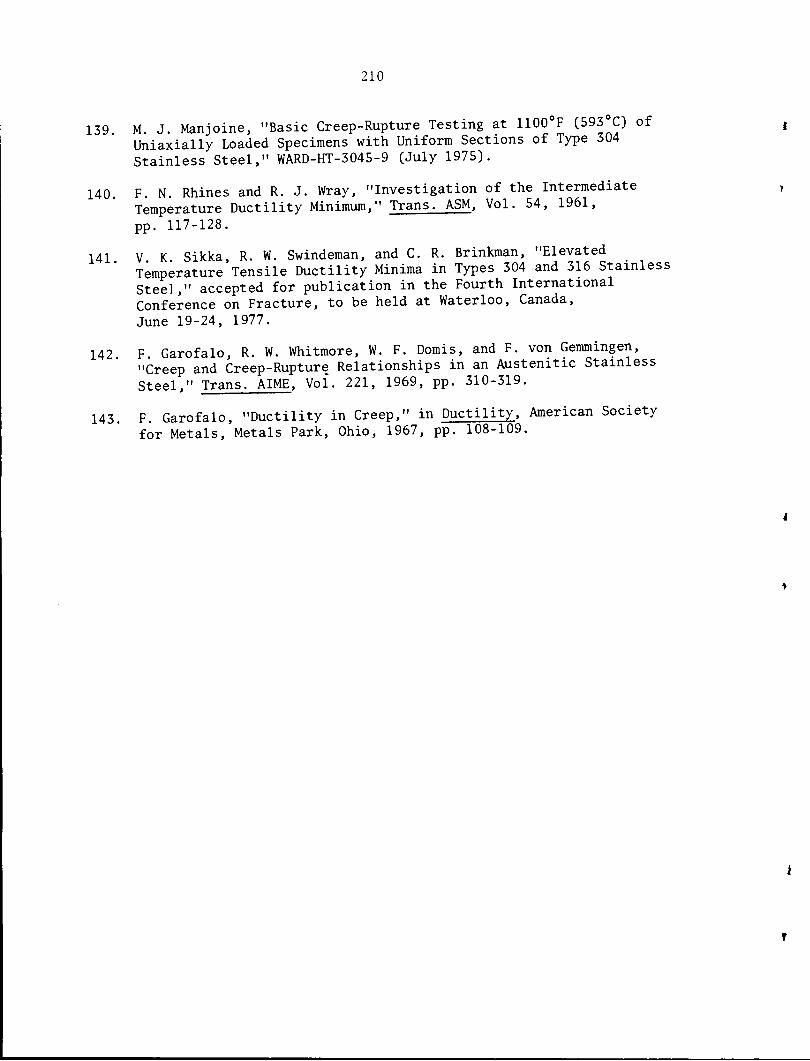
210
139 M J. Manjoine, "Basic Creep-Rupture Testing at 1100 F (593 C) ofUniaxially Loaded Specimens with Uniform Sections of Type 304Stainless Steel," WARD-HT-3045-9 (July 1975).
140. F. N. Rhines and R. J. Wray, "Investigation of the IntermediateTemperature Ductility Minimum," Trans. ASM, Vol. 54, 1961,pp. 117-128.
141 V K Sikka, R. W. Swindeman, and C. R. Brinkman, "ElevatedTemperature Tensile Ductility Minima in Types 304 and 316 StainlessSteel," accepted for publication in the Fourth InternationalConference on Fracture, to be held at Waterloo, Canada,June 19-24, 1977.
142 F. Garofalo, R. W. Whitmore, W. F. Domis, and F. von Gemmingen,"Creep and Creep-Rupture Relationships in an Austenitic StainlessSteel," Trans. AIME, Vol. 221, 1969, pp. 310-319.
143. F. Garofalo, "Ductility in Creep," in Ductility, American Societyfor Metals, Metals Park, Ohio, 1967, pp. 108-109.

1-2.
3.
4-10.
11.
12.
13.
14.
15-24.
25.
26.
27.
28.
29.
30.
31.
32.
33.
34.
35-37.
38.
39.
40.
41.
42.
43.
211
ORNL/TM-6110Distribution
Category
UC-79b, -h, -k
INTERNAL DISTRIBUTION
Central Research LibraryDocument Reference Section
Laboratory Records DepartmentLaboratory Records, ORNL RCORNL Patent Office
G. M. Adamson, Jr.S. E. Beall
M. K. Booker
C. R. Brinkman
A. Canonico
A. Conlin
M. Corum
J. E. CunninghamW. R. Gall
G. M. Goodwin
W. L. Greenstreet
W. 0. Harms
T. L. Hebble
M. R. Hill
Hammond
Hobson
P. R. Kasten
R. T. King
R. L. Klueh
A. L. Lotts
D.
J.
J.
J. P
D. 0
44. K. C. Liu
45. R. E. MacPherson
46. W. R. Martin (Y-12)47. H. E. McCoy, Jr.48. H. C. McCurdy49. C. J. McHargue50. H. Postma
51. P. Patriarca
52. C. E. Pugh53. J. L. Scott
54. V. K. Sikka
55. G. M. Slaughter56. J. P. Strizak
57. R. W. Swindeman
58. D. B. Trauger59. W. E. Unger60. J. R. Weir, Jr.61. G. D. Whitman
62. R. W. Balluffi (consultant)63. Paul M. Brister (consultant)64. W. R. Hibbard, Jr. (consultant)65. Hayne Palmour III (consultant)66. N. E. Promisel (consultant)67. D. F. Stein (consultant)
EXTERNAL DISTRIBUTION
68-69. DOE DIVISION OF REACTOR RESEARCH AND DEVELOPMENT,Washington, DC 20545
70-73. DOE DIVISION OF WASTE MANAGEMENT, PRODUCTION AND REPROCESSING,Washington, DC 20545
Chief, Industrial Programs BranchChief, Projects BranchChief, Technology Branch
74-75. DOE OAK RIDGE OPERATIONS OFFICE, P.O. Box E, Oak Ridge, TN 37830
Director, Reactor Division
Director, Research and Technical Support Division

212
76-339. DOE TECHNICAL INFORMATION CENTER, Office of Information Services,P.O. Box 62, Oak Ridge, TN 37830
For distribution as shown in TID-4500 Distribution Category,UC-79b (Fuels and Materials Engineering Development);UC-79h (Structural Materials Design Engineering); UC-79k(Components)
A US.GOVERNMENT PRINTING OFFICE: 1977-748-189/336


