UDC 519.632.4Algorithms for Solving the Boundary-Value Problems for

Atomic Trimers in Collinear Configuration using theKantorovich Method

A. A. Gusev*, O. Chuluunbaatar*†,S. I. Vinitsky*‡, V. L. DerbovS

* Joint Institute for Nuclear Research, Dubna, Russia† Institute of Mathematics, National University of Mongolia, Ulan-Bator, Mongolia

‡ RUDN University (Peoples’ Friendship University of Russia), Moscow, RussiaS Saratov State University, Saratov, Russia

The model of atomic trimers with molecular pair interactions for collinear configuration isformulated as a 2D boundary-value problem (BVP) in the Jacobi and polar coordinates. Thelatter is reduced to a 1D BVP for a system of second-order ordinary differential equations(ODEs) by means of the Kantorovich method using the expansion of the desired solutions overa set of angular basis functions, parametrically dependent on the (hyper)radial variable. Thealgorithms for solving the 1D parametric BVP by means of the finite element method (FEM)and calculating the asymptotes of the parametric angular functions and effective potentials of thesystem of ODEs at large values of the parameter are presented. The efficiency of the algorithmsis confirmed by comparing the calculated asymptotic solutions and effective potentials withthose of the parametric eigenvalue problem obtained by applying the FEM at large values of theparameter. The applicability of the algorithms is demonstrated by calculating the asymptoticexpansions of the parametric BVP solution, effective potentials and sets of binding energies forthe beryllium trimer in the collinear configuration.

Key words and phrases: boundary-value problems, the Kantorovich method systems ofsecond-order ordinary differential equations, finite element method

1. Introduction

At the present time, the processes of resonance scattering of diatomic molecules byatoms via three-particle clustering and metastable states, as well as the processes ofdissociation of the molecule induced by collisions with atoms are a subject of intensetheoretical and experimental studies [1–3].

To analyse such processes they use triatomic model systems with the atoms bound bypair realistic molecular and van-der-Waals potentials, which possess bound and metastablestates in the vicinity of the dissociation threshold of the diatomic molecule. The studyof such models stimulates the development of new methods and symbolic-numericalalgorithms for solving multidimensional boundary value problems with non-separablevariables and the construction of asymptotic states of the scattering problem in a systemof three atoms, based on the Kantorovich method and the finite element method (FEM),implemented in the problem-oriented software packages [4–9].

The aim of this paper is to formulate the 2D BVPs in the Jacobi and polar coordinatesfor the model of an atomic trimer in the collinear configuration and to develop thealgorithms for calculating the asymptotic parametric angular functions and the effectivepotentials arising in the Kantorovich method and needed for constructing the asymptoticstates of the triatomic scattering problem. The developed algorithms will be tested bythe example of beryllium atoms trimer model.

The paper is organised as follows. In Section 2 we set the 2D BVP. In Section 3 the2D BVP is reduced to the 1D BVP for a set of second-order ODEs using the Kantorovich

Received 16th September, 2016.The authors thank Profs. V.P. Gerdt, F.M. Penkov and Drs. P.M. Krassovitskiy, L.L. Hai for collaboration.The work was supported by the Russian Foundation for Basic Research (grants No. 14-01-00420, 17-01-00298). The reported study was funded within the Agreement N 02.a03.21.0008 dated 24.04.2016between the Ministry of Education and Science of the Russian Federation and RUDN University.

Gusev A.A. et al. Algorithms for Solving the Boundary-Value Problems for . . . 57

method. As an example, the eigenvalues and the hyperradial eigenfunction componentsare calculated by means of the Kantorovich method and FEM for the model of berylliumtrimer in the collinear configuration. In Section 4 we present the algorithms for calculatingthe asymptotes of the parametric basis functions in polar coordinates at large values ofthe parameter (hyperradial variable) and the effective potentials of the system of ODEs.In Conclusion the results and perspectives are discussed.

2. Setting of the problem

Consider a 2D model of three identical particles with the mass 𝑀 and the coordinates𝑥𝑖 ∈ R1, 𝑖 = 1, 2, 3, coupled via the pair potential 𝑉 (|𝑥𝑖 − 𝑥𝑗 |) 𝑖, 𝑗 = 1, 2, 3. Performingthe change of variables at cyclic permutation (𝛼, 𝛽, 𝛾) = (1, 2, 3):

𝑥 ≡ 𝑥(𝛼𝛽) = 𝑥𝛼 − 𝑥𝛽, 𝑦 ≡ 𝑦(𝛼𝛽)𝛾 =𝑥𝛼 + 𝑥𝛽 − 2𝑥𝛾√

3, 𝑥0 =

√2√3

(𝑥1 + 𝑥2 + 𝑥3),

we arrive at the Schrodinger equation for the wave function in the center-of-mass system𝑥𝑖 ∈ R1|𝑥1 + 𝑥2 + 𝑥3 = 0(

− 𝜕2

𝜕𝑦2− 𝜕2

𝜕𝑥2+

𝑀

~2(𝑉 (𝑥, 𝑦) − )

)Ψ(𝑦, 𝑥) = 0. (1)

In the case of a diatomic molecule with identical nuclei coupled via the pair potential𝑉 (|𝑥1 − 𝑥2|) and moving in the external potential field 𝑉 𝑏(|𝑥𝑖 − 𝑥3|), 𝑖 = 2, 1 of the thirdatom having the infinite mass, the same equation (1) is valid for the variables

𝑥 = 𝑥1 − 𝑥2, 𝑦 = 𝑥1 + 𝑥2,

the origin of the coordinate frame being placed on the infinite-mass atom, 𝑥3 = 0.Here the potential function for a trimer with the pair potentials (below this case is

referred to as Task 2),

𝑉 (𝑥, 𝑦)=𝑉 (|𝑥|)+𝑉(𝑥−√

3𝑦

2

)+ 𝑉

(𝑥 +√

3𝑦

2

), (2)

or the potential function for a dimer in the field of barrier potentials (below this case isreferred to as Task 3)

𝑉 (𝑥, 𝑦)=𝑉 (|𝑥|)+𝑉 𝑏(𝑥−𝑦

2

)+𝑉 𝑏

(𝑥+𝑦

2

), (3)

is symmetric with respect to the straight line 𝑥 = 0 (i.e., 𝑥1 = 𝑥2), which allows oneto consider the solutions of the problem in the half-plane 𝑥 > 0. Using the Dirichlet orNeumann boundary condition at 𝑥 = 0 allows one to obtain the solutions, symmetricand antisymmetric with respect to the permutation of two particles. If the pair potentialpossesses a high maximum in the vicinity of the pair collision point, then the solution ofthe problem in the vicinity of 𝑥 = 0 is exponentially small and can be considered in thehalf-plane 𝑥 > 𝑥min. In this case setting the Neumann or Dirichlet boundary conditionat 𝑥min gives only a minor contribution to the solution. The equation, describing themolecular subsystem (dimer), has the form(

− d2

d𝑥2+

𝑀

~2(𝑉 (𝑥) − 𝜀)

)𝜑(𝑥) = 0. (4)

58 Bulletin of PFUR. SeriesMathematics. Information Sciences. Physics. No 4, 2016. Pp. 56–76

We assume that the dimer has the discrete spectrum, consisting of a finite number 𝑛0> 1of bound states with the eigenfunctions 𝜑𝑗(𝑥), 𝑗 = 1, 𝑛0 and eigenvalues 𝜀𝑗 = −|𝜀𝑗 |< 0,and the continuous spectrum of eigenvalues 𝜀 > 0 with the corresponding eigenfunctions𝜑𝜀(𝑥). As a rule, the solutions of the discrete and continuum spectra of the BVP forEq. (4) can be found only numerically, except simplified models having exact solutionsand used for computer modelling of bimolecular chemical reactions. In certain cases theeigenfunctions of the continuous spectrum are approximated by the eigenfunctions ofpseudostates of discrete spectrum 𝜀𝑗 > 0, 𝑗 = 1 + 𝑛0, . . . calculated in sufficiently largebut finite interval [10].

The proposed algorithm is illustrated by the example of the molecular interactionapproximated by the Morse potential of Be2 with the reduced mass 𝑀/2 = 4.506 Da ofthe nuclei [10, 11]

𝑉 (𝑥) =𝑀

~2𝑉 (𝑥), 𝑉 (𝑥) = 𝐷exp[−2(𝑥− 𝑒𝑞)𝛼] − 2 exp[−(𝑥− 𝑒𝑞)𝛼]. (5)

Here 𝛼 = 2.96812 A−1 is the potential well width, 𝑒𝑞 = 2.47 A is the average

distance between the nuclei, and 𝐷 = 1280 K (1 K=0.184766 A−2,1 A−2=5.412262 K)is the potential well depth. This potential supports five bound states [12] having theenergies 𝜀𝑖 = (𝑀/~2)𝜀𝑖, 𝑖 = 1, . . . , 𝑛0 = 5 presented in Table 1. The parameter values aredetermined from the condition (𝜀2 − 𝜀1)/(2𝜋~𝑐) = 277.124cm−1, 1K/(2𝜋~ c)=0.69503476cm−1.

Table 1The discrete spectrum energies of dimer Be2 and the binding energy

𝐸𝑏 = −(𝐸 − 𝐸𝑎) of gerade (𝑔) and ungerade (𝑢) states of trimer Be3 counted of𝐸𝑎 = 𝜀1 = −193.06A−2 = −1044K dimer energy Be2 calculated in grid

Ω𝜌 = 4.1(20)7(10)10 at 𝑗max = 10

−𝜀𝑖 𝐸𝑏𝑖,𝑔 𝐸𝑏

𝑖,𝑢

−𝜀1=1044.879 649K 𝐸𝑏1,𝑔 = 196.02A−2 = 1060.86K 𝐸𝑏

1,𝑢 = 107.52A−2 = 581.90K

−𝜀2=646.157 093K 𝐸𝑏2,𝑔 = 142.37A−2 = 770.51K 𝐸𝑏

2,𝑢 = 67.41A−2 = 364.84K

−𝜀3=342.791 979K 𝐸𝑏3,𝑔 = 93.95A−2 = 508.50K 𝐸𝑏

3,𝑢 = 34.60A−2 = 187.28K

−𝜀4=134.784305K 𝐸𝑏4,𝑔 = 52.77A−2 = 285.63K 𝐸𝑏

4,𝑢 = 11.79A−2 = 63.83K

−𝜀5=22.134 073K 𝐸𝑏5,𝑔 = 32.32A−2 = 174.95K 𝐸𝑏

5,𝑢 = 0.8A−2 = 4.4K

𝐸𝑏6,𝑔 = 22.31A−2 = 120.75K

𝐸𝑏7,𝑔 = 5.14A−2 = 27.87K

To solve the discrete spectrum problem we applied the FEM of the seventh or-der using the Hermitian interpolation polynomials with double nodes [9]. The grid𝑥0, . . . , 𝑥𝑖, . . . , 𝑥𝑛 was used to calculate the values of both the function and its deriva-tives.

3. Reduction of the BVP using the Kantorovich method

Using the change of variables 𝑥 = 𝜌 sin𝜙, 𝑦 = 𝜌 cos𝜙, we rewrite Eq. (1) in polarcoordinates (𝜌, 𝜙), Ω𝜙,𝜌 = (𝜌 ∈ (0,∞), 𝜙 ∈ (0, 2𝜋))(

−1

𝜌

𝜕

𝜕𝜌𝜌𝜕

𝜕𝜌+

1

𝜌2Λ(𝜙, 𝜌) − 𝐸

)Ψ(𝜙, 𝜌) = 0, Λ(𝜙, 𝜌) = − d2

d𝜙2+𝜌2𝑉 (𝜙, 𝜌), (6)

Gusev A.A. et al. Algorithms for Solving the Boundary-Value Problems for . . . 59

where for a trimer with pair potentials

𝑉 (𝜙, 𝜌)=𝑉 (𝜌| sin𝜙|) + 𝑉 (𝜌| sin(𝜙− 2𝜋/3)|) + 𝑉 (𝜌| sin(𝜙− 4𝜋/3)|), (7)

and for a dimer with pair potential in the external field of barrier potentials:

𝑉 (𝜙, 𝜌)=𝑉 (𝜌| sin𝜙|) + 𝑉 𝑏(𝜌| sin(𝜙− 𝜋/4)|) + 𝑉 𝑏(𝜌| sin(𝜙 + 𝜋/4)|). (8)

The solution of Eq. (6) is sought in the form of the Kantorovich expansion

Ψ𝑖𝑜(𝜙, 𝜌) =

𝑗max∑𝑗=1

𝜑𝑗(𝜙; 𝜌)𝜒𝑗𝑖𝑜(𝜌). (9)

Here 𝜒𝑗𝑖𝑜(𝜌) are unknown functions and the orthogonal normalised angular basisfunctions 𝜑𝑗(𝜙; 𝜌) ∈ 𝐿2(Ω) in the interval Ω = 𝜙 ∈ (0, 2𝜋) are defined as eigenfunctions,corresponding to the eigenvalues of the Sturm-Liouville problem for the equation

(Λ(𝜙, 𝜌)−𝜀𝑗(𝜌))𝜑𝑗(𝜙; 𝜌) = 0,

2𝜋∫0

d𝜙𝜑𝑖(𝜙; 𝜌)𝜑𝑗(𝜙; 𝜌)=𝛿𝑖𝑗 , (10)

where 𝜀𝑗(𝜌), 𝑗 = 1, . . . is the set of the real-valued eigenvalues forming a purely discretespectrum at each value of the parameter 𝜌 ∈ (0,+∞). For the problems under consid-eration the potential function 𝑉 (𝜙, 𝜌) depending on the parameter 𝜌 can be defined asfollows.

Task 1. The case of one pair potential in the intervals 𝜙 ∈ (0, 2𝜙𝛼) (𝜙𝛼=𝜋/3, 𝜋/4 or𝜋/2) 𝑉 (𝜙, 𝜌)=𝑉 (𝜌 sin𝜙).

Task 2. The case of three pair potentials, Eq. (7), in the interval 𝜙 ∈ (0, 2𝜙𝛼=𝜋/3).

Task 3. The case of one pair potential and two penetrable or almost impenetrablebarrier potentials, Eq. (8), in the interval 𝜙 ∈ (0, 𝜙𝛼 = 𝜋/2) or in the intervals 𝜙 ∈(0, 𝜙𝛼 = 𝜋/4 − 𝜖) and 𝜙 ∈ (𝜙𝛼 = 𝜋/4 − 𝜖, 𝜋/2), 0 < 𝜖 ≪ 𝜋/4.

The solutions symmetric with respect to the permutation of two particles satisfy theNeumann boundary condition at 𝜙 = 0 and 𝜙 = 2𝜙𝛼. If the pair potential possesses a highpeak in the vicinity of the pair collision point, then the solution of the problem (6) willbe considered in the half-plane Ω𝜙,𝜌 = (𝜌 ∈ (𝜌min,∞), 𝜙 ∈ [𝜙min(𝜌), 2𝜙𝛼 − 𝜙min(𝜌)]) withthe Neumann or Dirichlet boundary condition. Since the potential of the boundary-valueproblem (10) is symmetric with respect to 𝜙 = 𝜙𝛼, the gerade 𝜑𝑗(𝜙; 𝜌) = 𝜑𝑗(2𝜙𝛼 − 𝜙; 𝜌)and ungerade 𝜑𝑗(𝜙; 𝜌) = −𝜑𝑗(2𝜙𝛼 − 𝜙; 𝜌) solutions, satisfying the Neumann or theDirichlet boundary condition respectively, will be considered separately in the interval𝜙 ∈ [𝜙min(𝜌), 𝜙𝛼]. The parametric angular basis functions with successive numbers𝑗 = 1, . . . , 𝑛0 are referred to as cluster states with 𝜀𝑗(𝜌) < 0 and those with 𝑗 > 𝑛0 + 1 aspseudostates with 𝜀𝑗(𝜌) > 0 corresponding to discrete and continuous spectrum of (4) atlarge values of the parameter 𝜌, respectively.

The system of coupled ODEs in the Kantorovich form has the form[−1

𝜌

d

d𝜌𝜌

d

d𝜌+

𝜀𝑖(𝜌)

𝜌2− 𝐸

]𝜒𝑖𝑖𝑜(𝜌) +

𝑗max∑𝑗=1

𝑊𝑖𝑗(𝜌)𝜒𝑗𝑖𝑜(𝜌) = 0, (11)

𝑊𝑖𝑗(𝜌) = 𝐻𝑗𝑖(𝜌) +1

𝜌

d

d𝜌𝜌𝑄𝑗𝑖(𝜌) + 𝑄𝑗𝑖(𝜌)

d

d𝜌. (12)

60 Bulletin of PFUR. SeriesMathematics. Information Sciences. Physics. No 4, 2016. Pp. 56–76

Here the potential curves (terms) 𝜀𝑗(𝜌) are eigenvalues of the BVP (10) and the effectivepotentials 𝑄𝑖𝑗(𝜌) = −𝑄𝑗𝑖(𝜌), 𝐻𝑖𝑗(𝜌) = 𝐻𝑗𝑖(𝜌) are given by the integrals calculated usingthe above symmetry on reduced intervals 𝜙 ∈ [0, 2𝜙𝛼]:

𝑄𝑖𝑗(𝜌) = −2𝜙𝛼∫0

d𝜙𝜑𝑖(𝜙; 𝜌)d𝜑𝑗(𝜙; 𝜌)

d𝜌,𝐻𝑖𝑗(𝜌) =

2𝜙𝛼∫0

d𝜙d𝜑𝑖(𝜙; 𝜌)

d𝜌

d𝜑𝑗(𝜙; 𝜌)

𝑑𝜌. (13)

For Task 3 the effective potentials 𝑖𝑗(𝜌) = 𝑊𝑖𝑗(𝜌) + 𝑉 𝑏𝑖𝑗(𝜌) are sums of 𝑊𝑖𝑗(𝜌),

calculated using the potential curves and the parametric basis functions of Task 1, andthe integrals of barrier potentials 𝑉 𝑏

𝑖𝑗(𝜌) multiplied by the basis functions

𝑉 𝑏𝑖𝑗(𝜌) =

𝜙𝛼∫0

d𝜙𝜑𝑖(𝜙; 𝜌)(𝑉 𝑏(𝜌 sin(𝜙− 𝜋/4)) + 𝑉 𝑏(𝜌 sin(𝜙 + 𝜋/4)))𝜑𝑗(𝜙; 𝜌).

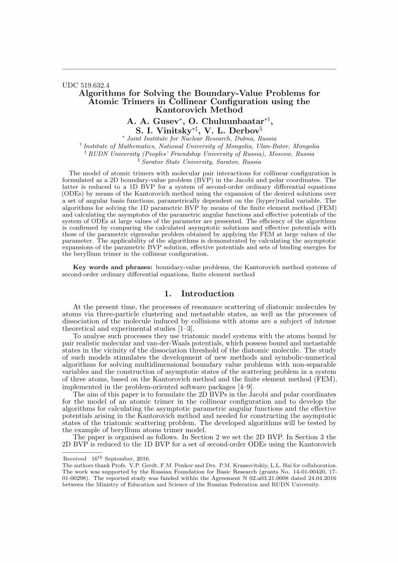
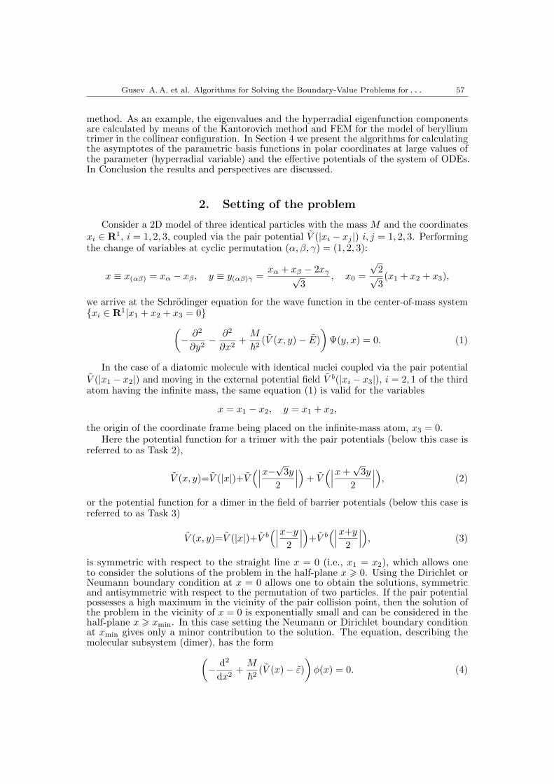
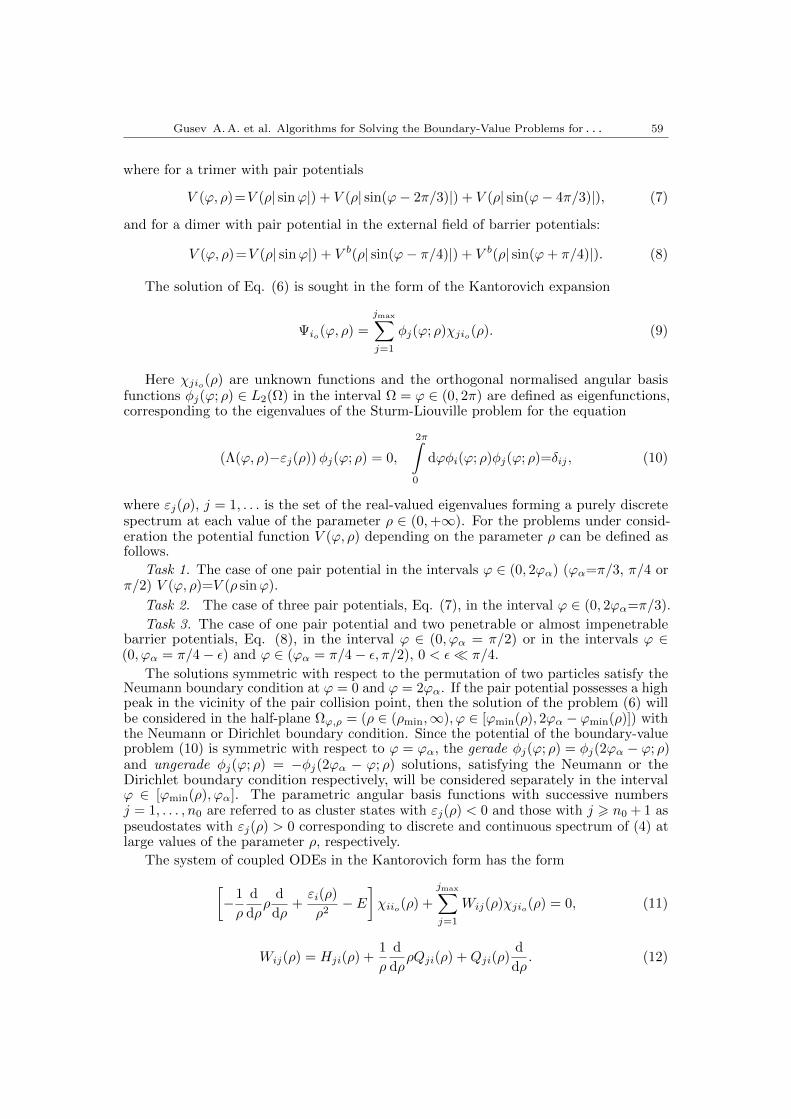
As an example, we calculated with a required accuracy the parametric basis functionsof BVP (10) and the effective potentials (13) for the models of Be2 dimer and Be3 trimerin collinear configuration by means the FEM using the programme ODPEVP [4]. Theresults of calculation on the grid Ω𝜙[1.8/𝜌, 𝑎] = 1.8/𝜌(24)3/𝜌(10)4/𝜌(5)5/𝜌(10)𝑎 for𝑎 = 𝜋/2 for Be2 dimer and 𝑎 = 𝜋/6 for Be3 trimer are shown in Figs. 1, 2, and 3.

(a) (b)

Figure 1. The potential curves of Be2 (in K, 1K=0.18A−2), i.e., the energyeigenvalues depending upon the parameter 𝜌 (in A): (a) 𝜀𝑗(𝜌) and (b) 𝜀𝑗 = 𝜀𝑗(𝜌)/𝜌

2.Here 𝑗 = 1, . . . , 10

In the FEM the eigenfunctions 𝜑(𝜙; 𝜌) of the problem (10) are approximated by afinite sum of local functions 𝑁𝑝

𝑙 (𝜙) with coefficients 𝜑𝑙(𝜙𝑝𝑠,𝑟, 𝜌) specified in the nodes 𝜙𝑝

𝑠,𝑟

of the finite element grid [4]

𝜑(𝜙; 𝜌) =𝐿∑

𝑙=0

𝜑𝑙(𝜙𝑝𝑠,𝑟, 𝜌)𝑁𝑝

𝑙 (𝜙). (14)

Gusev A.A. et al. Algorithms for Solving the Boundary-Value Problems for . . . 61

(a)

(b)

(c)

(d)

Figure

2.Be+Be2:Thepote

ntialcurv

esofBe3(in

K),

i.e.,

theenerg

yeigenvaluesdependingupon

thepara

mete

r𝜌(in

A):

(a)𝜀 𝑗(𝜌)and

(b)𝜀 𝑗=𝜀 𝑗(𝜌)/𝜌2,(c)th

eisolinesof2D

pote

ntials

ofBe3trim

er,

and

(d)th

ediagonaleffectivepote

ntials

𝐻𝑗𝑗(𝜌).

Here

𝑗=

1,...,10

(a)

(b)

(c)

(d)

Figure

3.Theeffectivepote

ntials

(13)(a

)𝐻

𝑗𝑗−1(𝜌),

(b)𝑄

𝑗𝑗−1(𝜌),

(c)𝐻

𝑗1(𝜌),

(d)𝑄

𝑗1(𝜌).

Here

𝑗=

2,...,10

62 Bulletin of PFUR. SeriesMathematics. Information Sciences. Physics. No 4, 2016. Pp. 56–76

The functions 𝑁𝑝𝑙 (𝜙)𝐿𝑙=0, 𝐿 = 𝑛𝑝, form a basis in the space of polynomials of the 𝑝-th

order. After substituting the expansion (14) into the variational functional correspondingto BVP (10) and minimizing it [13,14] we obtain the generalized eigenvalue problem

A𝑝𝜑ℎ = 𝜖ℎB𝑝𝜑ℎ. (15)

Here A𝑝 is the stiffness matrix; B𝑝 is the positive definite mass matrix; 𝜑ℎ is thevector approximating the solution on the finite-element grid; and 𝜖ℎ is the correspondingeigenvalue [4]. The required accuracy of the calculated eigenvalues, eigenfunctions andtheir derivatives with respect to parameter, and effective potentials is provided by theestimations given below.

Let 𝜖𝑗(𝜌), 𝜑𝑗(𝜙; 𝜌) be the exact solution of (10) and 𝜖ℎ𝑗 , 𝜑ℎ𝑗 be the numerical solution

of (15). Then for a bounded positively defined operator Λ(𝜙; 𝜌) the following estimatesare valid [13]

|𝜖𝑗(𝜌) − 𝜖ℎ𝑗 | 6 𝑐1ℎ2𝑝,𝜑𝑗(𝜙; 𝜌) − 𝜑ℎ

𝑗

06 𝑐2ℎ

𝑝+1, 𝑐1 > 0, 𝑐2 > 0, (16)

where ||𝑣(𝜙; 𝜌)||20 =𝜙max∫𝜙min

𝑣2(𝜙; 𝜌)d𝜙; ℎ is the maximal grid step, 𝑝 is the order of finite

elements, 𝑗 is the number of the corresponding eigensolution, and the constants 𝑐1 and 𝑐2do not depend on the step ℎ. It is necessary to mention that the second estimate of Eq.(16) is valid also for the solution 𝜕𝜑𝑗(𝜙; 𝜌)/𝜕𝜌 of the problem [4]

(Λ(𝜙, 𝜌)−𝜀𝑗(𝜌))𝜕𝜑𝑗(𝜙; 𝜌)

𝜕𝜌= −

(𝜕Λ(𝜙, 𝜌)

𝜕𝜌−𝜕𝜀𝑗(𝜌)

𝜕𝜌

)𝜑𝑗(𝜙; 𝜌),

2𝜋∫0

d𝜙𝜑𝑖(𝜙; 𝜌)𝜕𝜑𝑗(𝜙; 𝜌)

𝜕𝜌=0.

(17)

This fact guarantees the same accuracy for eigenfunctions and their derivatives withinthe present method.

Theorem 1. Let Λ(𝜙; 𝜌) be a bounded positively defined operator on the finite interval𝜙 ∈ (𝜙min, 𝜙max). Let 𝜕𝑉 (𝜙, 𝜌)/𝜕𝜌 be also bounded for each value of the parameter 𝜌.Then for the exact solutions, 𝜕𝜖𝑗(𝜌)/𝜕𝜌, 𝜕𝜑𝑗(𝜙; 𝜌)/𝜕𝜌 ∈ ℋ2, from (17) and the potentialmatrix elements, 𝑄𝑖𝑗(𝜌), 𝐻𝑖𝑗(𝜌), from (13), and the corresponding numerical values,

𝜕𝜖ℎ𝑗 /𝜕𝜌, 𝜕𝜑ℎ𝑗 /𝜕𝜌 ∈ ℋ1, and 𝑄ℎ

𝑖𝑗, 𝐻ℎ𝑖𝑗, the following estimates are valid [4]

𝜕𝜖𝑗(𝜌)

𝜕𝜌−

𝜕𝜖ℎ𝑗𝜕𝜌

6 𝑐3ℎ

2𝑝,

𝜕𝜑𝑗(𝜙; 𝜌)

𝜕𝜌−

𝜕𝜑ℎ𝑗

𝜕𝜌

0

6 𝑐4ℎ𝑝+1,

𝑄𝑖𝑗(𝜌) −𝑄ℎ𝑖𝑗

6 𝑐5ℎ

2𝑝,𝐻𝑖𝑗(𝜌) −𝐻ℎ

𝑖𝑗

6 𝑐6ℎ

2𝑝,

(18)

where ℎ is the maximal grid step, 𝑝 is the order of finite elements, 𝑖, 𝑗 are the numbersof the corresponding solutions, and the constants 𝑐3, 𝑐4, 𝑐5 and 𝑐6 do not depend on thestep ℎ.

For this model the eigenvalues and the hyperradial components of 2D eigenfunctionsof the BVP for the set of ODEs (11) with Neumann boundary conditions were calcu-lated with the required accuracy by means the FEM using the program KANTBP [9].The discrete energy spectrum of the dimer Be2 calculated of the grid Ω𝑥(1.8, 10) =

Gusev A.A. et al. Algorithms for Solving the Boundary-Value Problems for . . . 63

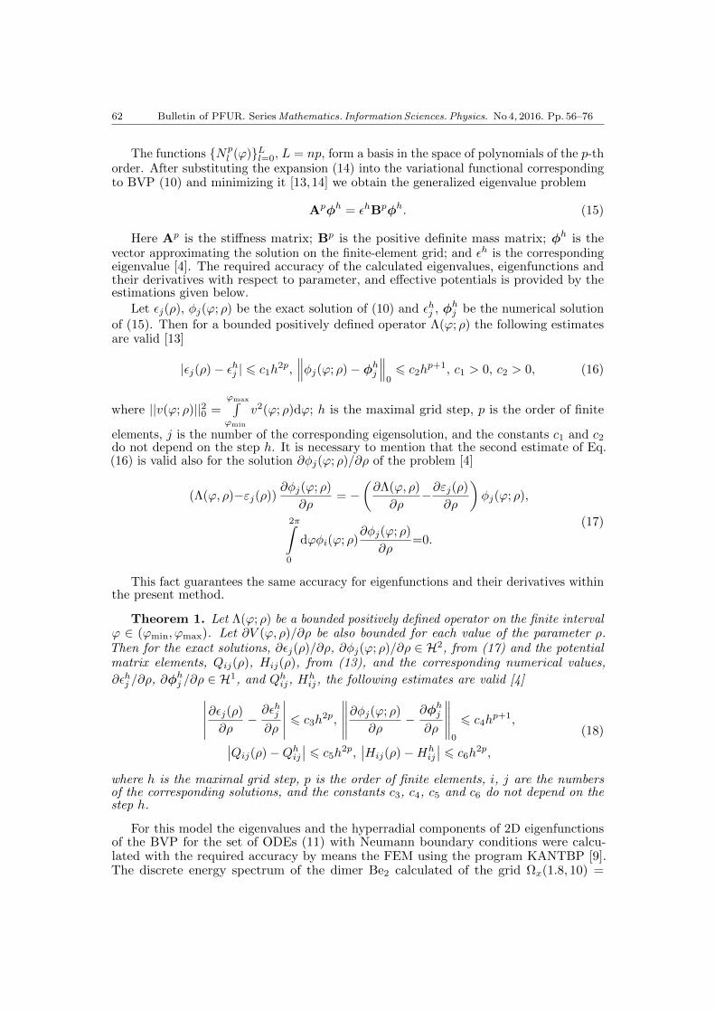
1.8(24)3(10)4(5)5(10)10 and the set of binding energies of the trimer Be3 calculated ofthe grid Ω𝜌 = 4.1(20)7(10)10 with the eighth-order Lagrange elements (𝑝 = 8) are shownin Table 1, and the components of the trimer eigenfunctions (9) are shown in Fig. 4.

Figure 4. Components 𝜒𝑖,𝜎=𝑔,𝑢𝑗 (𝜌,𝐸) ≡ 𝜒

(𝑖)𝑗 (𝜌) of gerade (𝑔) and ungerade (𝑢) bound

states of the trimer Be3 with total energy 𝐸 in A−2

4. Algorithms for calculating the asymptotes of parametricangular basis functions and effective potentials

Algorithm for calculating the cluster parametric angular basis functions and effectivepotentials of the lower part of the discrete spectrum

Let us calculate the solution of the Sturm-Liouville problem (10) at large 𝜌

(Λ(𝜙; 𝜌)−𝜀𝑗(𝜌))𝜑𝑗(𝜙; 𝜌)≡(− 𝜕2

𝜕𝜙2+𝜌2𝑉 (𝜌 sin𝜙)−𝜀𝑗(𝜌)

)𝜑𝑗(𝜙; 𝜌)=0. (19)

Using the new variable 𝑥′ defined as 𝜙 = 𝑥′/𝜌, 𝑥′ = 𝜌 arcsin(𝑥/𝜌) we get(− 𝜕2

𝜕𝑥′2+ 𝑉 (𝜌 sin(𝑥′/𝜌)) − 𝜀𝑗(𝜌)

𝜌2

)𝜑𝑗(𝑥

′; 𝜌) = 0. (20)

In the argument of the potential we add and subtract 𝑥′ and expand the potential inTaylor series in the vicinity of 𝑥′,

𝑉 (𝜌 sin(𝑥′/𝜌)) = 𝑉 (𝑥′ + ∆𝑥′)) = 𝑉 (𝑥′) +∑𝑘=1

d𝑘𝑉 (𝑥′)

d𝑥′𝑘(∆𝑥′)𝑘

𝑘!, (21)

64 Bulletin of PFUR. SeriesMathematics. Information Sciences. Physics. No 4, 2016. Pp. 56–76

where the small correction ∆𝑥′ = 𝜌 sin(𝑥′/𝜌) − 𝑥′ ≪ 1 is presented in the form of Taylorseries

∆𝑥′ =∑𝑘=1

(−1)𝑘

(2𝑘 + 1)!

𝑥′2𝑘+1

𝜌2𝑘.

Then the Sturm-Liouville problem (19) is reduced to(− 𝜕2

𝜕𝑥′2+ 𝑉 (𝑥′) +

∑𝑘=1

𝑉 (𝑘)(𝑥′)

𝜌2𝑘− 𝜀𝑗(𝜌)

𝜌2

)𝜑𝑗(𝑥

′; 𝜌) = 0,

⟨𝜑𝑖(𝜌)|𝜑𝑗(𝜌)⟩ ≡𝑥′max∫

𝑥′0

d𝑥′(𝜑𝑖(𝑥′; 𝜌)𝜑𝑗(𝑥

′; 𝜌) = 𝛿𝑖𝑗 .

(22)

Here first terms 𝑉 (𝑘)(𝑥′) of the asymptotic expansion of 𝑉 (𝜌 sin(𝑥′/𝜌)) read as

𝑉 (1)(𝑥′)=−𝑥′3

6

d𝑉 (𝑥′)

d𝑥′ ,

𝑉 (2)(𝑥′)=𝑥′5

360

(5𝑥′ d

2𝑉 (𝑥′)

d𝑥′2+3

d𝑉 (𝑥′)

d𝑥′

),

𝑉 (3)(𝑥′)=− 𝑥′7

45360

(35𝑥′2 d3𝑉 (𝑥′)

d𝑥′3+63𝑥′ d

2𝑉 (𝑥′)

d𝑥′2+9

d𝑉 (𝑥′)

d𝑥′

),

𝑉 (4)(𝑥′)=𝑥′9

5443200

(175𝑥′3 d4𝑉 (𝑥′)

d𝑥′4+630𝑥′2 d3𝑉 (𝑥′)

d𝑥′3+369𝑥′ d

2𝑉 (𝑥′)

d𝑥′2+15

d𝑉 (𝑥′)

d𝑥′

).

(23)

Note that 𝑘!𝑉 (𝑘)(𝑥′) are the derivatives of the potential of the BVP (22) with respectto the parameter 𝜌−2. So, we apply the modified version of the program ODPEVP forcalculating the parameter derivatives of the solution up to the given order to determinethe asymptotic expansion of the cluster eigenfunctions and eigenvalues.

In the framework of FEM using similar expansions (14) we reduce the eigenvalueproblem on the given finite-element grid Ω𝑥′(𝑥′

min, 𝑥′max) in the finite interval 𝑥′ ∈

(𝑥′min, 𝑥

′max) to a generalized eigenvalue algebraic problem with respect to the eigenvalues

𝜆 ∈ 𝜆𝑗𝑁𝑜𝑗=1 and the corresponding eigenvectors 𝑐(𝜌) = (𝑐𝑖(𝜌))𝑗𝑁𝑜

𝑗=1 of the order 𝐿. In

the considered example Ω𝑥′(1.8, 10) = 1.8(24)3(10)4(5)5(10)10 with Lagrange elementsof the eighth order NPOL=p=8 (the numbers of elements between the nodes given inparentheses), providing the accuracy 𝑂(ℎ2𝑝) for the eigenvalues and 𝑂(ℎ𝑝+1) ≈ 10−8 forthe eigenfunctions, ℎ being the maximal grid step. 𝐿 equals the number of grid nodes,which in the considered example was 𝐿 = 393.

𝐴(𝜌)𝑐(𝜌) − 𝑐(𝜌)𝐵𝜆(𝜌) = 0, (24)

(𝑐(𝜌))𝑇𝐵𝑐(𝜌) = 1. (25)

Here the matrix 𝐴(𝜌) is presented in the form of inverse power series

𝐴(𝜌) = 𝐴(0) +

𝑘max∑𝑘=1

𝜌−2𝑘

𝑘!𝐴(𝑘). (26)

Gusev A.A. et al. Algorithms for Solving the Boundary-Value Problems for . . . 65

We choose as unperturbed the matrix operator 𝐴(0) corresponding to the differential

one, − 𝜕2

𝜕𝑥′2 + 𝑉 (𝑥′), and numerically solve the corresponding algebraic problem

𝐴(0)𝑐(0) − 𝜆(0)𝐵𝑐(0) = 0, 𝑐(0)𝑇𝐵𝑐(0) = 1. (27)

The solution 𝜆(𝜌), 𝑐(𝜌) is sought in the form of inverse power series

𝜆(𝜌) = 𝜆(0)𝑗 (𝜌) +

𝑘max∑𝑘=1

𝜌−2𝑘

𝑘!𝜆(𝑘)𝑗 , 𝑐(𝜌) = 𝑐(0) +

𝑘max∑𝑘=1

𝜌−2𝑘

𝑘!𝑐(𝑘). (28)

The substitution of Eq. (28) into Eq. (22) leads to the system of inhomogeneousalgebraic equations for the corrections 𝜆(𝑘) and 𝑐(𝑘):

(𝐴(0)𝑐(𝑘) − 𝜆(0)𝐵𝑐(𝑘)) + (𝐴(𝑘)𝑐(0) − 𝜆(𝑘)𝐵𝑐(0)) = 𝑏(𝑘),

𝑏(𝑘) ≡𝑘−1∑𝑛=1

𝑘!

𝑛!(𝑘 − 𝑛)!(𝐵𝑐(𝑘−𝑛)𝜆(𝑛) −𝐴(𝑛)𝑐(𝑘−𝑛)), 𝑏(1) ≡ 0,

𝐴(𝑘) ≡ 𝜕𝑘𝐴(0)

𝜕𝑟𝑘, 𝜆(𝑘) ≡ 𝜕𝑘𝜆(0)

𝜕𝑟𝑘.

(29)

Differentiating the normalization condition (25), we obtain additional conditions forthe corrections 𝑐(𝑘):

𝑐(0)𝑇𝐵𝑐(𝑘) ≡ 𝐹

(𝑘)𝑁 = −1

2

𝑘−1∑𝑛=1

𝑘!

𝑛!(𝑘 − 𝑛)!𝑐(𝑘−𝑛)𝑇𝐵𝑐(𝑛).

Multiplying (29) by 𝑐(0)𝑇

and taking the zero values of the first term and the nor-malization condition into account, we get the formula for the corrections 𝜆(𝑘) of theeigenvalues:

𝜆(𝑘) = 𝑐(0)𝑇𝐴(𝑘)𝑐(0) − 𝑐(0)

𝑇𝑏(𝑘). (30)

The vector 𝑐(𝑘) is calculated by solving the system of algebraic equations

𝐾𝑐(𝑘) ≡ 𝐴(0)𝑐(𝑘) − 𝜆(0)𝐵𝑐(𝑘) = 𝑏(𝑘)

𝑏(𝑘) ≡ −𝑘∑

𝑛=1

𝑘!

𝑛!(𝑘 − 𝑛)!(𝐴(𝑛)𝑐(𝑘−𝑛) − 𝜆(𝑛)𝐵𝑐(𝑘−𝑛)),

𝑘∑𝑛=0

𝑘!

𝑛!(𝑘 − 𝑛)!𝑐(𝑘−𝑛)𝑇𝐵𝑐(𝑛) = 0,

(31)

where the latter equation is a result of differentiation of the normalization condition.

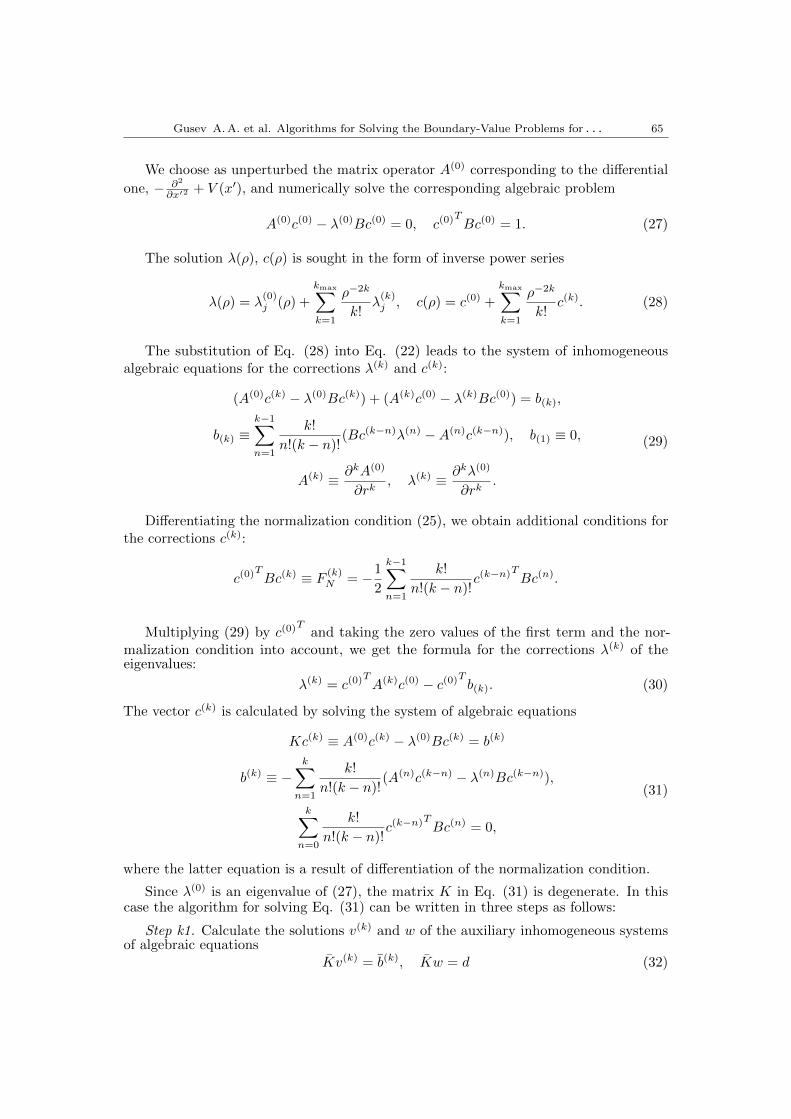
Since 𝜆(0) is an eigenvalue of (27), the matrix 𝐾 in Eq. (31) is degenerate. In thiscase the algorithm for solving Eq. (31) can be written in three steps as follows:

Step k1. Calculate the solutions 𝑣(𝑘) and 𝑤 of the auxiliary inhomogeneous systemsof algebraic equations

𝑣(𝑘) = (𝑘), 𝑤 = 𝑑 (32)

66 Bulletin of PFUR. SeriesMathematics. Information Sciences. Physics. No 4, 2016. Pp. 56–76

with the non-degenerate matrix and the right-hand sides (𝑘) and 𝑑

𝑖𝑗 =

𝐾𝑖𝑗 , (𝑖− 𝑠)(𝑗 − 𝑠) = 0,

𝛿𝑖𝑗 , (𝑖− 𝑠)(𝑗 − 𝑠) = 0,

(𝑘)𝑗 =

𝑏(𝑘)𝑗 , 𝑗 = 𝑠,

0, 𝑗 = 𝑠,𝑑𝑗 =

𝐾𝑗𝑠, 𝑗 = 𝑠,

0, 𝑗 = 𝑠,

where 𝑠 is the number of vector 𝑐(0) element having the maximal absolute value.

Step k2. Evaluate the coefficient 𝛾(𝑘)

𝛾(𝑘) = −𝛾(𝑘)1 − 𝐹

(𝑘)𝑁

(𝑐(0)𝑠 − 𝛾2)

, 𝛾(𝑘)1 = 𝑣(𝑘)

𝑇𝑐(0), 𝛾2 = 𝑤𝑇 𝑐(0). (33)

Step k3. Evaluate the vector 𝑐(𝑘)𝑗

𝑐(𝑘)𝑗 =

𝑣(𝑘)𝑗 − 𝛾(𝑘)𝑤𝑗 , 𝑗 = 𝑠,

𝛾(𝑘), 𝑗 = 𝑠.(34)

The execution of the above procedure yields the required asymptotic expansion forthe eigenvalues

𝜀𝑗(𝜌)

𝜌2= 𝜀

(0)𝑗 (𝜌) +

𝑘max∑𝑘=1

𝜌−2𝑘𝜀(𝑘)𝑗 = 𝜆

(0)𝑗 (𝜌) +

𝑘max∑𝑘=1

𝜌−2𝑘

𝑘!𝜆(𝑘)𝑗 (35)

and the corresponding expansion of the eigenfunctions in the nodes 𝑥′𝑖 of the given grid

𝜑𝑗(𝑥′𝑖; 𝜌) = (𝑐(0))𝑖𝑗 +

𝑘max∑𝑘=1

𝜌−2𝑘

𝑘!(𝑐(𝑘))𝑖𝑗 .

Following Eq. (14) we present it in the form of a piecewise-polynomial function

𝜑𝑗(𝑥′ ∈ [𝑥′

𝑝𝑘, 𝑥′𝑝(𝑘+1)]; 𝜌) =

𝑝∑𝑝′=0

𝜑𝑗(𝑥′𝑝𝑘+𝑝′ ; 𝜌)

𝑝∏𝑝′′=0,𝑝′′ =𝑝′

𝑥′ − 𝑥′𝑝′′

𝑥′𝑝′ − 𝑥′

𝑝′′. (36)

We calculate the discrete spectrum solutions 𝜑𝑗(𝜙; 𝜌) of the problem (19) on the grid𝜙𝑖 = 𝑥′

𝑖/𝜌, related to the solutions 𝜑𝑗(𝑥′𝑖; 𝜌) of the problem (20) as

𝜑𝑗(𝜙𝑖 = 𝑥′𝑖/𝜌; 𝜌) =

√𝜌𝜑𝑗(𝑥

′𝑖; 𝜌).

The corresponding piecewise-polynomial functions are

𝜑𝑗(𝜙𝑖 ∈ [𝜙𝑝𝑘, 𝜙𝑝(𝑘+1)]; 𝜌)𝑟=𝜑𝑗(𝜙𝑖=𝑥′𝑖/𝜌 ∈ [𝑥′

𝑝𝑘/𝜌, 𝑥′𝑝(𝑘+1)/𝜌]; 𝜌) =

=

𝑝∑𝑝′=0

𝜑𝑗(𝜙𝑝𝑘+𝑝′ ; 𝜌)

𝑝∏𝑝′′=0

𝑝′′ =𝑝′

𝜙−𝜙𝑝′′

𝜙𝑝′−𝜙𝑝′′=

𝑝∑𝑝′=0

𝜑𝑗(𝜙𝑝𝑘+𝑝′ ; 𝜌)

𝑝∏𝑝′′=0

𝑝′′ =𝑝′

𝜙𝜌−𝑥′𝑝′′

𝑥′𝑝′−𝑥′

𝑝′′=

Gusev A.A. et al. Algorithms for Solving the Boundary-Value Problems for . . . 67

=√𝜌

𝑝∑𝑝′=0

𝜑𝑗(𝑥′𝑝𝑘+𝑝′ ; 𝜌)

𝑝∏𝑝′′=0

𝑝′′ =𝑝′

𝜙𝜌−𝑥′𝑝′′

𝑥′𝑝′−𝑥′

𝑝′′=

=√𝜌

𝑝∑𝑝′=0

((𝑐(0))𝑖𝑗+

𝑘𝑚𝑎𝑥∑𝑘=1

𝜌−2𝑘

𝑘!(𝑐(𝑘))𝑖𝑗

)𝑝∏

𝑝′′=0

𝑝′′ =𝑝′

𝜙𝜌−𝑥′𝑝′′

𝑥′𝑝′−𝑥′

𝑝′′. (37)

The nodes 𝑥′𝑝′ in Eq. (37) are the same as in Eq. (36).

The calculation of the matrix elements is similar to the derivation of Newton-Cotesformulae [15]. In each of the subintervals of the nonuniform finite element mesh thecalculated values of functions and their derivatives are approximated, in the consideredcase of Ω𝜙[1.8/𝜌, 10/𝜌] = 1.8/𝜌(24)3/𝜌(10)4/𝜌(5)5/𝜌(10)10/𝜌 by a Lagrange polynomialof the order 𝑝 = 8, which provides the same relative accuracy of 𝑂(ℎ𝑝+1). The obtainedapproximations of functions are polynomials of 𝜙, explicitly depending on 𝜌. By analyticaldifferentiation of Eq. (37) with respect to the parameter we arrive at the explicit

expansion of the derivative𝜕𝜑𝑗(𝜙;𝜌)

𝜕𝜌 . Integrating the products of functions 𝜑𝑗(𝜙; 𝜌) and/or

their parametric derivatives in each subinterval of the length ℎ𝑖 = 𝜙𝑝(𝑖+1) − 𝜙𝑝𝑖 of thenonuniform finite element mesh Ω𝜙 and summing the obtained results, we get the requiredasymptotic expansion of matrix elements (13) for cluster states, 𝑖, 𝑗 = 1, . . . , 𝑛0:

𝑄𝑖𝑗(𝜌) =

𝑘𝑚𝑎𝑥∑𝑘=1

𝑄(2𝑘−1)𝑖𝑗

𝜌2𝑘−1, 𝐻𝑖𝑗(𝜌) =

𝑘𝑚𝑎𝑥∑𝑘=1

𝐻(2𝑘)𝑖𝑗

𝜌2𝑘. (38)

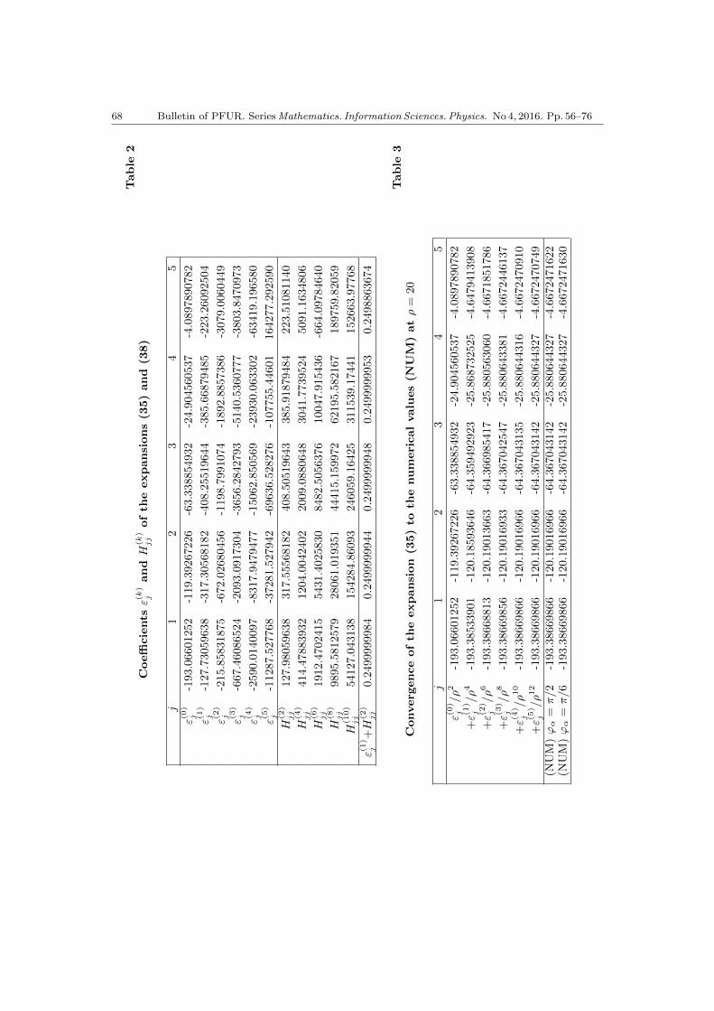
For the beryllium trimer in collinear configuration, the coefficients 𝜀(𝑘)𝑗 of the expansion

(35) and the coefficients 𝐻(𝑘)𝑗𝑗 of the expansion (38) at 𝑖 = 𝑗 are presented in Table 2, and

the first coefficients of the expansions (38) are

𝑄(1)𝑖𝑗 =

⎛⎜⎜⎜⎜⎝0 10.3201 −3.81790 1.83170 −.903311

−10.3201 0 12.2419 −5.54402 2.68986

3.81790 −12.2419 0 11.5096 −5.30745

−1.83170 5.54402 −11.5096 0 7.99437

0.903311 −2.68986 5.30745 −7.99437 0

⎞⎟⎟⎟⎟⎠ ,

𝑄(3)𝑖𝑗 =

⎛⎜⎜⎜⎜⎝0 19.6114 −3.63427 1.58999 −6.31271

−19.6114 0 32.2355 −12.5531 22.0625

3.63427 −32.2355 0 52.0431 −53.8134

−1.58999 12.5531 −52.0431 0 105.275

6.31271 −22.0625 53.8134 −105.275 0

⎞⎟⎟⎟⎟⎠ ,

𝑄(5)𝑖𝑗 =

⎛⎜⎜⎜⎜⎝0 68.2366 −6.68774 −14.8770 128.505

−68.2366 0 91.6918 27.6600 −356.227

6.68774 −91.6918 0 68.9065 595.104

14.8770 −27.6600 −68.9065 0 −523.035

−128.505 356.227 −595.104 523.035 0

⎞⎟⎟⎟⎟⎠ ,

68 Bulletin of PFUR. SeriesMathematics. Information Sciences. Physics. No 4, 2016. Pp. 56–76

Table

2Coefficients

𝜀(𝑘)

𝑗and

𝐻(𝑘

)𝑗𝑗

ofth

eexpansions(3

5)and

(38)

𝑗1

23

45

𝜀(0)

𝑗-193.06601252

-119.39267226

-63.338854932

-24.904560537

-4.0897890782

𝜀(1)

𝑗-127.73059638

-317.30568182

-408.25519644

-385.66879485

-223.26092504

𝜀(2)

𝑗-215.85831875

-672.02680456

-1198.7991074

-1892.8857386

-3079.0060449

𝜀(3)

𝑗-667.46086524

-2093.0917304

-3656.2842793

-5140.5360777

-3803.8470973

𝜀(4)

𝑗-2590.0140097

-8317.9479477

-15062.850569

-23930.063302

-63419.196580

𝜀(5)

𝑗-11287.527768

-37281.527942

-69636.528276

-107755.44601

164277.292590

𝐻(2

)𝑗𝑗

127.98059638

317.55568182

408.50519643

385.91879484

223.51081140

𝐻(4

)𝑗𝑗

414.47883932

1204.0042402

2009.0880648

3041.7739524

5091.1634806

𝐻(6

)𝑗𝑗

1912.4702415

5431.4025830

8482.5056376

10047.915436

-664.09784640

𝐻(8

)𝑗𝑗

9895.5812579

28061.019351

44415.159972

62195.582167

189759.82059

𝐻(1

0)

𝑗𝑗

54127.043138

154284.86093

246059.16425

311539.17441

152663.97768

𝜀(1)

𝑗+𝐻

(2)

𝑗𝑗

0.2499999984

0.2499999944

0.2499999948

0.2499999953

0.2498863674

Table

3Converg

enceofth

eexpansion

(35)to

thenumericalvalues(N

UM

)at𝜌=

20

𝑗1

23

45

𝜀(0)

𝑗/𝜌2

-193.06601252

-119.39267226

-63.338854932

-24.904560537

-4.0897890782

+𝜀(

1)

𝑗/𝜌4

-193.38533901

-120.18593646

-64.359492923

-25.868732525

-4.6479413908

+𝜀(

2)

𝑗/𝜌6

-193.38668813

-120.19013663

-64.366985417

-25.880563060

-4.6671851786

+𝜀(

3)

𝑗/𝜌8

-193.38669856

-120.19016933

-64.367042547

-25.880643381

-4.6672446137

+𝜀(

4)

𝑗/𝜌10

-193.38669866

-120.19016966

-64.367043135

-25.880644316

-4.6672470910

+𝜀(

5)

𝑗/𝜌12

-193.38669866

-120.19016966

-64.367043142

-25.880644327

-4.6672470749

(NUM)𝜙

𝛼=

𝜋/2

-193.38669866

-120.19016966

-64.367043142

-25.880644327

-4.6672471622

(NUM)𝜙

𝛼=

𝜋/6

-193.38669866

-120.19016966

-64.367043142

-25.880644327

-4.6672471630

Gusev A.A. et al. Algorithms for Solving the Boundary-Value Problems for . . . 69

𝐻(2)𝑖𝑗 =

⎛⎜⎜⎜⎜⎝127.981 −67.2820 −85.3811 73.3913 −44.4889

−67.2820 317.556 −161.487 −40.5195 46.8714

−85.3811 −161.487 408.505 −231.091 45.2520

73.3913 −40.5195 −231.091 385.919 −215.798

−44.4889 46.8714 45.2520 −215.798 223.511

⎞⎟⎟⎟⎟⎠ ,

𝐻(4)𝑖𝑗 =

⎛⎜⎜⎜⎜⎝414.479 −142.333 −526.641 464.604 −624.169

−142.333 1204.00 −420.171 −812.366 1119.09

−526.641 −420.171 2009.09 −947.285 −464.551

464.604 −812.366 −947.285 3041.77 −2605.05

−624.169 1119.09 −464.551 −2605.05 5091.16

⎞⎟⎟⎟⎟⎠ ,

𝐻(6)𝑖𝑗 =

⎛⎜⎜⎜⎜⎝1912.47 −670.689 −2112.77 815.251 4153.61

−670.689 5431.40 −1689.40 −3295.46 −646.435

−2112.77 −1689.40 8482.51 −2016.27 −12077.1

815.251 −3295.46 −2016.27 10047.9 12431.9

4153.61 −646.435 −12077.1 12431.9 −664.074

⎞⎟⎟⎟⎟⎠ .

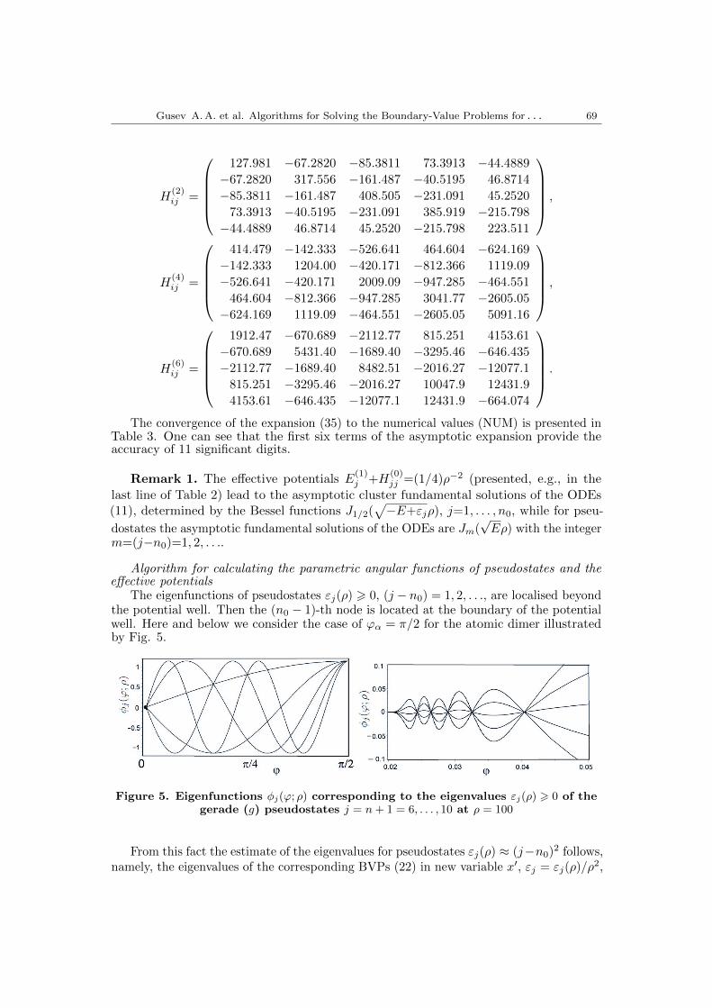
The convergence of the expansion (35) to the numerical values (NUM) is presented inTable 3. One can see that the first six terms of the asymptotic expansion provide theaccuracy of 11 significant digits.

Remark 1. The effective potentials 𝐸(1)𝑗 +𝐻

(0)𝑗𝑗 =(1/4)𝜌−2 (presented, e.g., in the

last line of Table 2) lead to the asymptotic cluster fundamental solutions of the ODEs(11), determined by the Bessel functions 𝐽1/2(

√−𝐸+𝜀𝑗𝜌), 𝑗=1, . . . , 𝑛0, while for pseu-

dostates the asymptotic fundamental solutions of the ODEs are 𝐽𝑚(√𝐸𝜌) with the integer

𝑚=(𝑗−𝑛0)=1, 2, . . ..

Algorithm for calculating the parametric angular functions of pseudostates and theeffective potentials

The eigenfunctions of pseudostates 𝜀𝑗(𝜌) > 0, (𝑗 − 𝑛0) = 1, 2, . . ., are localised beyondthe potential well. Then the (𝑛0 − 1)-th node is located at the boundary of the potentialwell. Here and below we consider the case of 𝜙𝛼 = 𝜋/2 for the atomic dimer illustratedby Fig. 5.

Figure 5. Eigenfunctions 𝜑𝑗(𝜙; 𝜌) corresponding to the eigenvalues 𝜀𝑗(𝜌) > 0 of thegerade (𝑔) pseudostates 𝑗 = 𝑛+ 1 = 6, . . . , 10 at 𝜌 = 100

From this fact the estimate of the eigenvalues for pseudostates 𝜀𝑗(𝜌) ≈ (𝑗−𝑛0)2 follows,namely, the eigenvalues of the corresponding BVPs (22) in new variable 𝑥′, 𝜀𝑗 = 𝜀𝑗(𝜌)/𝜌2,

70 Bulletin of PFUR. SeriesMathematics. Information Sciences. Physics. No 4, 2016. Pp. 56–76

will be a small quantity (see Fig. 1b). So, the solution 𝜀𝑛(𝜌) (𝜀𝑛 = 𝜀𝑛(𝜌)/𝜌2) of thederived equation is sought in the form of a power series at 𝑛/𝜌 < 1

𝜀𝑛(𝜌) = 𝑛2+

𝑘max∑𝑘=1

𝜀(𝑘)𝑛

𝜌𝑘. (39)

Then the numerical values of the function 𝐵(𝜙𝑖; 𝜌) = 𝐵(𝑥′𝑖) and its derivative

𝐵′(𝜙𝑖; 𝜌) = 𝜌𝐵′(𝑥′𝑖) on the specified grid Ω𝜙 = 𝜙1 = 𝜙0, . . . , 𝜙𝑖 = 𝑥𝑖/𝜌, . . . , 𝜙𝑁 = 𝜙𝜀 in

the polar system of coordinates are determined via the values of the function 𝐵(𝑥𝑖) andits derivative 𝐵′(𝑥𝑖) on the grid Ω𝑥′

𝑖𝑥′

1 = 𝑥′0, . . . , 𝑥

′𝑖, . . . , 𝑥

′𝑁 = 𝑥′

𝜀, found with the sameaccuracy accepted in the FEM scheme chosen above in the form of the power series ofthe small parameter 𝜀𝑛:

𝐵𝑗(𝑥𝑖)=𝐵(0)𝑖 +

𝑘max∑𝑘=1

𝐵(𝑘)𝑖 (𝜀

(1)𝑛 , . . . , 𝜀

(𝑘)𝑛 )

𝜌𝑘, 𝐵′

𝑗(𝑥𝑖)=𝑏(0)𝑖 +

𝑘max∑𝑘=1

𝑏(𝑘)𝑖 (𝜀

(1)𝑛 , . . . , 𝜀

(𝑘)𝑛 )

𝜌𝑘, (40)

using the Runge–Kutta method, in which the all terms contain the power 𝑘max + 1 of

1/𝜌 and the higher ones are neglected. The expansion coefficients 𝐵(𝑘)𝑖 ≡ 𝐵

(𝑘)𝑖 (𝑥′

𝑖) and

𝑏(𝑘)𝑖 ≡ 𝑏

(𝑘)𝑖 (𝑥′

𝑖), calculated at the grid nodes 𝑥′𝑖 for the BVP (22) with the potential 𝑉 (𝑥′)

defined in Eq. (5) are presented in Fig. 6.

Figure 6. Expansion coefficients 𝐵(𝑘)𝑖 (𝜀

(1)𝑛 , . . . , 𝜀

(𝑘)𝑛 ) and 𝑏

(𝑘)𝑖 (𝜀

(1)𝑛 , . . . , 𝜀

(𝑘)𝑛 ), 𝑘=0, 2, 3, 4, 5,

𝑛 = 1 with 𝜀(𝑘)𝑛 given by Eq. (44) calculated at the nodes 𝑥′

𝑖 of the grid Ω𝑥′

One can see that in the vicinity of the potential well the corrections to the eigenfunctions

are small, and at large 𝑥′ they become essential. The coefficient 𝑏(0)𝑖 , the derivative of

the wave function with 𝜀𝑛 = 0, exponentially tends to a constant for 𝑥 > 5.5. Fromthese observations the condition for choosing 𝑥𝜀 follows. However, to avoid analyticalcalculations of the exponential terms in the effective potentials (13) between the weaklybound cluster states and pseudostates, it is sufficient to choose 𝑥′

𝜀 = 10.The interval 𝜙0 6 𝜙 6 𝜋/2 is divided into two subintervals by the point 𝜙𝜀 = 𝑥𝜀/𝜌:

𝜙0 < 𝜙 6 𝜙𝜀 and 𝜋/2 > 𝜙 > 𝜙𝜀. In the calculations the point 𝑥𝜀 was chosen from thecondition |𝑉 (𝑥 > 𝑥𝜀)| < 𝜀, where 𝜀 is a preassigned number, and the left-hand boundaryof the interval 𝜙0 = 0. In the case of a high barrier, at the pair collision point, when theeigenfunctions in its vicinity are close to zero, the left boundary of the interval changes,

Gusev A.A. et al. Algorithms for Solving the Boundary-Value Problems for . . . 71

𝜙0 = 𝑥0/𝜌 > 0. The eigenfunctions 𝜑𝑗(𝜙; 𝜌) are calculated in the form

𝜑𝑗(𝜙; 𝜌) =

𝐴𝑗(𝜌)𝐵𝑗(𝜙; 𝜌), 𝜙0 6 𝜙 6 𝜙𝜀,

𝐶𝑗(𝜌)√

2𝜋

cossin

(√

𝜀𝑗(𝜌)(𝜙− 𝜋/2)), 𝜙𝜀 < 𝜙 6 𝜋/2,

2

∫ 𝜋/2

𝜙0

d𝜙(𝜑𝑛(𝜙; 𝜌))2 = 1.

(41)

Here 𝐴𝑗(𝜌) and 𝐶𝑗(𝜌) are the normalisation factors, and 𝐵(𝜙; 𝜌) is determined fromthe numerical solution 𝐵(𝑥) in Cartesian coordinates using the transformation 𝜙 = 𝑥/𝜌.From the continuity of the eigenfunctions and their derivatives,

𝜑𝑛(𝜙𝜀 − 0; 𝜌) = 𝜑𝑛(𝜙𝜀 + 0; 𝜌),

d𝜑𝑛

d𝜙(𝜙𝜀 − 0; 𝜌) =

d𝜑𝑛

d𝜙(𝜙𝜀 + 0; 𝜌),

(42)

we get the equation for the eigenvalue 𝜀𝑛(𝜌):tan(

√𝜀𝑛(𝜌)(𝜙𝜀−𝜋

2 )) even 𝑛

−cot(√𝜀𝑛(𝜌)(𝜙𝜀−𝜋

2 )) odd 𝑛

−√𝜀𝑛(𝜌)

𝑅=0,

𝑅=𝐵′

𝑛(𝜙𝜀; 𝜌)

𝐵𝑛(𝜙𝜀; 𝜌)=𝜌𝐵′

𝑛(𝑥𝜀)

𝐵𝑛(𝑥𝜀).

(43)

Substitute (40) into (43), and then substitute (39) into the resulting equation. Ex-panding both sides of the equation in inverse powers of 𝜌, we arrive at the system of linear

equations, from which the expansion coefficients 𝜀(𝑘)𝑛 , and then the coefficients 𝐴𝑛(𝜌) and

𝐶𝑛(𝜌) are determined.

Since the values of the function 𝐵𝑛(𝜙; 𝜌) and its derivative 𝐵′𝑛(𝜙; 𝜌) on the grid Ω𝜙

are known, for the calculation of the first integral we use the quadrature formula of theNewton-Cotes type. The second integral is calculated analytically using the expansion(39). We have the analytical expression in the interval 𝜙𝜀(𝜌) < 𝜙 6 𝜋/2, and the explicitdependence of its values upon the parameter 𝜌 on the grid Ω𝜙. For the consideredpotential (5) we get the asymptotes of the 𝑔 and 𝑢 potential curves at 𝑛 = 𝑗 − 𝑛0 for𝑛/𝜌 < 1:

𝜀𝑛(𝜌)=𝑛2+

𝑘max∑𝑘=1

𝜀(𝑘)𝑛

𝜌𝑘; for 𝑔-parity at odd 𝑛, or 𝑢-parity at even 𝑛. (44)

The first terms of these expansions are expressed as

𝜀(1)𝑛 =4.4862257𝑛2, 𝜀(2)𝑛 =15.094666𝑛2,

𝜀(3)𝑛 =−88.164324𝑛2+0.2988408𝑛4, 𝜀(4)𝑛 =−770.50344𝑛2+3.3516683𝑛4,

𝜀(5)𝑛 =−13803.854𝑛2+162.14850𝑛4−0.2922734𝑛6,

𝜀(6)𝑛 =−68926.763𝑛2+1584.0782𝑛4−4.4329308𝑛6.

The calculated eigenvalues in comparison with the numerical solution obtained bymeans of the program ODPEVP [4] are presented in Table 4.

72 Bulletin of PFUR. SeriesMathematics. Information Sciences. Physics. No 4, 2016. Pp. 56–76

Table 4Convergence of the expansion (44) at 𝜌=50 and the numerical results (NUM)

gerade (𝑔-parity)𝑛 1 3 5 7𝑛2 1.000000 9.00000 25.00000 49.00000

+𝜀(1)𝑛 /𝜌 1.089724 9.80752 27.24311 53.39650

+𝜀(2)𝑛 /𝜌2 1.095762 9.86186 27.39405 53.69235

+𝜀(3)𝑛 /𝜌3 1.095059 9.85570 27.37792 53.66353

+𝜀(4)𝑛 /𝜌4 1.094936 9.85464 27.37517 53.65878

+𝜀(5)𝑛 /𝜌5 1.094893 9.85428 27.37437 53.65775

+𝜀(6)𝑛 /𝜌6 1.094888 9.85425 27.37432 53.65774

(NUM) 1.094887 9.85424 27.37431 53.65776

ungerade (𝑢-parity)𝑛 2 4 6 8𝑛2 4.000000 16.00000 36.000000 64.0000

+𝜀(1)𝑛 /𝜌 4.358898 17.43559 39.230082 69.7423

+𝜀(2)𝑛 /𝜌2 4.383049 17.53219 39.447445 70.1287

+𝜀(3)𝑛 /𝜌3 4.380266 17.52152 39.425152 70.0934

+𝜀(4)𝑛 /𝜌4 4.379781 17.51968 39.421409 70.0877

+𝜀(5)𝑛 /𝜌5 4.379613 17.51911 39.420448 70.0868

+𝜀(6)𝑛 /𝜌6 4.379597 17.51906 39.420407 70.0868

(NUM) 4.379592 17.51905 39.420408 70.0869

The described algorithm is implemented in the Maple-Fortran environment. Theasymptotic expansions, obtained using it at 𝜌 = 50, coincide with the numerical solutiongiven by the finite element method to 5–6 significant digits for the eigenvalues and to 4–5significant digits for the eigenfunctions. The asymptotes of the effective potentials (13)between the states 𝑛1 = 𝑖 − 𝑛0 and 𝑛2 = 𝑗 − 𝑛0 of the same (𝑔 or 𝑢) parity at 𝑛0 = 5,𝑖, 𝑗 = 𝑛0 + 1, . . . for 𝑛/𝜌 < 1 have the form:

𝑄𝑛1𝑛2(𝜌)=

𝑘max∑𝑘=0

𝑄(𝑘+2)𝑛1𝑛2

𝜌𝑘+2, 𝐻𝑛1𝑛2

(𝜌)=

𝑘max∑𝑘=0

𝐻(𝑘+4)𝑛1𝑛2

𝜌𝑘+4. (45)

First terms of these expansions read as

𝑄(2)𝑛1𝑛2

=2.2431128𝑛1𝑛2

(𝑛21−𝑛2

2), 𝑄(3)

𝑛1𝑛2=5.0315554

𝑛1𝑛2

(𝑛21−𝑛2

2),

𝑄(4)𝑛1𝑛2

=188.67822𝑛1𝑛2

(𝑛21−𝑛2

2)+0.22413

𝑛1𝑛2(𝑛21−𝑛2

2)

(𝑛21−𝑛2

2),

𝐻(4)𝑛1𝑛2

=10.06311𝑛1𝑛2(𝑛2

1+𝑛22)

(𝑛21−𝑛2

2)2, 𝐻(5)

𝑛1𝑛2=45.14538

𝑛1𝑛2(𝑛21+𝑛2

2)

(𝑛21−𝑛2

2)2+69.93509𝑛1𝑛2,

𝐻(6)𝑛1𝑛2

=−1642.273𝑛1𝑛2(𝑛2

1+𝑛22)

(𝑛21−𝑛2

2)2+8.044

𝑛31𝑛

32

(𝑛21−𝑛2

2)2,+476.762𝑛1𝑛2

Gusev A.A. et al. Algorithms for Solving the Boundary-Value Problems for . . . 73

𝐻(4)𝑛1𝑛1

=0.6289444+2.0691442𝑛21, 𝐻(5)

𝑛1𝑛1=2.8215867+79.217746𝑛2

1,

𝐻(6)𝑛1𝑛1

= − 102.642068 + 138.328874𝑛21 + 0.826991𝑛4

1.

Using Eq. (35) and Eq. (41), we get the asymptotic expansions for 𝑄𝑖𝑛(𝜌) and 𝐻𝑖𝑛(𝜌)between the cluster states 𝑖=1, . . . , 𝑛0 and pseudostates 𝑛−𝑛0=1, 2, . . . , for 𝑛/𝜌<1

𝑄𝑖𝑛(𝜌)=

𝑘max∑𝑘=0

𝑄(𝑘+5/2)𝑖𝑛

𝜌𝑘+5/2, 𝐻𝑖𝑛(𝜌)=

𝑘max∑𝑘=0

𝐻(𝑘+7/2)𝑖𝑛

𝜌𝑘+7/2, (46)

The first terms of these expansions read as

𝑄(5/2)1𝑛 =−0.428911𝑛, 𝑄

(7/2)1𝑛 =−1.443145𝑛, 𝑄

(9/2)1𝑛 =−25.01600𝑛+0.183791𝑛3,

𝑄(5/2)2𝑛 = 1.273900𝑛, 𝑄

(7/2)2𝑛 =+4.286254𝑛, 𝑄

(9/2)2𝑛 = 75.66328𝑛−0.546657𝑛3,

𝑄(5/2)3𝑛 =−2.497511𝑛, 𝑄

(7/2)3𝑛 =−8.403301𝑛, 𝑄

(9/2)3𝑛 =−152.3919𝑛+1.075421𝑛3,

𝑄(5/2)4𝑛 = 3.668834𝑛, 𝑄

(7/2)4𝑛 =+12.34441𝑛, 𝑄

(9/2)4𝑛 = 231.9007𝑛−1.599005𝑛3,

𝑄(5/2)5𝑛 =−4.098659𝑛, 𝑄

(7/2)5𝑛 =−13.79066𝑛, 𝑄

(9/2)5𝑛 =−247.9253𝑛+2.018873𝑛3,

𝐻(7/2)1𝑛 = 22.53006𝑛, 𝐻

(9/2)1𝑛 =+77.24936𝑛, 𝐻

(11/2)1𝑛 =1551.8678𝑛−9.835892𝑛3,

𝐻(7/2)2𝑛 =−26.57543𝑛, 𝐻

(9/2)2𝑛 =−93.70381𝑛, 𝐻

(11/2)2𝑛 =−2203.032𝑛+11.89657𝑛3,

𝐻(7/2)3𝑛 =−12.19890𝑛, 𝐻

(9/2)3𝑛 =−32.64199𝑛, 𝐻

(11/2)3𝑛 =262.11512𝑛+4.400493𝑛3,

𝐻(7/2)4𝑛 = 85.06821𝑛, 𝐻

(9/2)4𝑛 =+273.8820𝑛, 𝐻

(11/2)4𝑛 =4387.8346𝑛−35.91925𝑛3,

𝐻(7/2)5𝑛 =−120.4823𝑛, 𝐻

(9/2)5𝑛 =−391.5948𝑛, 𝐻

(11/2)5𝑛 =−8001.428𝑛+54.83111𝑛3.

5. Conclusion

The model for beryllium trimer in collinear configuration is formulated as a 2Dboundary-value problem for the Schrodinger equation in polar coordinates. This problemis reduced using the Kantorovich expansions to the boundary-value problem for a setof second-order ordinary differential equations. The symbolic-numeric algorithms areproposed and implemented in Maple to evaluate the asymptotic expansions (35), (38), (45)and (46) of the parametric BVP eigensolutions and the effective potentials 𝑊𝑖𝑗(𝜌) in inversepowers of 𝜌. It can be used for calculation of the asymptotes of the fundamental solutionsof the system of second-order ODEs at large values of 𝜌 [10] and construction of asymptoticstates of three atomic scatterring problem. The proposed approach can be applied to thefurther analysis of quantum transparency effect [10,11], quantum diffusion [16–18] andthe resonance scattering in triatomic systems using modern theoretical and experimentalresults [19–21] and algorithms and programs [4–9].

References

1. V. Efimov, Few-Body Physics: Giant Trimers True to Scale, Nature Phys. 5 (2009)533–534.

2. M. Zaccanti, B. Deissler, C. D’Errico, M. Fattori, Jona-Lasinio, S. M. Muller, G. Roati,M. Inguscio, M. G., Observation of an Efimov Spectrum in an Atomic System, NaturePhys. 5 (2009) 586–591.

74 Bulletin of PFUR. SeriesMathematics. Information Sciences. Physics. No 4, 2016. Pp. 56–76

3. J. Voigtsberger, et al., Imaging the Structure of the Trimer Systems 4He3 and 3He4He2,Nature Commun. 5 (2014) 5765.

4. O. Chuluunbaatar, A. A. Gusev, S. I. Vinitsky, A. G. Abrashkevich, ODPEVP: AProgram for Computing Eigenvalues and Eigenfunctions and Their First Derivativeswith Respect to the Parameter of the Parametric Self-Adjoined Sturm–LiouvilleProblem, Computer Physics Communications 180 (2009) 1358–1375.

5. A. A. Gusev, O. Chuluunbaatar, S. I. Vinitsky, A. G. Abrashkevich, POTHEA: AProgram for Computing Eigenvalues and Eigenfunctions and Their First Derivativeswith Respect to the Parameter of the Parametric Self-Adjoined 2D Elliptic PartialDifferential Equation, Comput. Phys. Commun. 185 (2014) 2636–2654.

6. A. A. Gusev, O. Chuluunbaatar, S. I. Vinitsky, A. G. Abrashkevich, Description of aProgram for Computing Eigenvalues and Eigenfunctions and Their First Derivativeswith Respect to the Parameter of the Coupled Parametric Self-Adjoined EllipticDifferential Equations, Bulletin of Peoples’ Friendship University of Russia. Series“Mathematics. Information Sciences. Physics” (2) (2014) 336–341.

7. O. Chuluunbaatar, A. A. Gusev, A. G. Abrashkevich, A. Amaya-Tapia, M. S. Kaschiev,S. Y. Larsen, S. I. Vinitsky, KANTBP: A Program for Computing Energy Levels,Reaction Matrix and Radial Wave Functions in the Coupled-Channel HypersphericalAdiabatic Approach, Comput. Phys. Commun. 177 (2007) 649–675.

8. O. Chuluunbaatar, A. A. Gusev, S. I. Vinitsky, A. G. Abrashkevich, KANTBP 2.0:New Version of a Program for Computing Energy Levels, Reaction Matrix and RadialWave Functions in the Coupled-Channel Hyperspherical Adiabatic Approach, Comput.Phys. Commun. 179 (2008) 685–693.

9. A. A. Gusev, L. L. Hai, O. Chuluunbaatar, S. I. Vinitsky, Program KANTBP 4M forSolving Boundary-Value Problems for Systems of Ordinary Differential Equations ofthe Second Order.URL http://wwwinfo.jinr.ru/programs/jinrlib/kantbp4m

10. S. I. Vinitsky, A. A. Gusev, O. Chuluunbaatar, L. Hai, V. Derbov, P. Krassovitskiy,A. Gozdz, Symbolic Numerical Algorithm for Solving Quantum Tunneling Problem ofa Diatomic Molecule Through Repulsive Barriers, Lect. Notes Comp. Sci. 8660 (2014)472–490.

11. P. M. Krassovitskiy, F. M. Pen’kov, Contribution of resonance tunneling of moleculeto physical observables, J. Phys. B 47 (2014) 225210.

12. J. Wang, G. Wang, J. Zhao, Density Functional Study of Beryllium Clusters withGradient Correction, J. Phys. Cond. Matt. 13 (2001) L753–L758.

13. G. Strang, G. J. Fix, An Analysis of the Finite Element Method, Prentice-Hall,Englewood Cliffs, New York, 1973.

14. K. J. Bathe, Finite Element Procedures in Engineering Analysis, Englewood Cliffs,Prentice Hall, New York, 1982.

15. I. S. Berezin, N. P. Zhidkov, Computing Methods, Vol. 1, Pergamon Press, Oxford,1965.

16. A. A. Gusev, L. L. Hai, Algorithm for Solving the Two-Dimensional Boundary ValueProblem for Model of Quantum Tunneling of a Diatomic Molecule Through RepulsiveBarriers, Bulletin of Peoples’ Friendship University of Russia. Series “Mathematics.Information Sciences. Physics” (1) (2015) 15–36.

17. E. Pijper, A. Fasolino, Quantum Surface Diffusion of Vibrationally Excited MolecularDimers, J. Chem. Phys. 126 (2007) 014708.

18. A. A. Gusev, A. Gozdz, V. L. Derbov, S. I. Vinitsky, O. Chuluunbaatar, P. M.Krassovitskiy, Models of Resonant Tunneling of Composite Systems Through RepulsiveBarriers, JINR News (1) (2014) 22–26.

19. A. V. Mitin, Ab Initio Calculations of Weakly Bonded He2 and Be2 Molecules byMRCI Method with Pseudo-Natural Molecular Orbitals, Int. J. Quantum Chem. 111(2011) 2560–2567.

20. J. M. Merritt, V. E. Bondybey, M. C. Heaven, Beryllium dimer—caught in the act ofbonding, Science 324 (2009) 1548–1551.

Gusev A.A. et al. Algorithms for Solving the Boundary-Value Problems for . . . 75

21. K. Patkowski, V. Spirko, K. Szalewicz, On the Elusive Twelfth Vibrational State ofBeryllium Dimer, Science 326 (2009) 1382–1384.

УДК 519.632.4Алгоритмы решения краевых задач для атомных тримеров в

коллинеарной конфигурации методом КанторовичаА. А. Гусев*, О. Чулуунбаатар*†, С. И. Виницкий*‡,

В. Л. ДербовS* Объединённый институт ядерных исследований, г. Дубна, Россия

† Институт математики, Монгольский государственный университет, Улан-Батор,Монголия

‡ Российский университет дружбы народов, Москва, РоссияS Саратовский государственный университет, г. Саратов, Россия

Модель атомных тримеров с парными молекулярными взаимодействиями в коллинеарнойконфигурации формулируется в виде двумерной краевой задачи в якобиевских полярныхкоординатах. Последняя сводится методом Канторовича к одномерной краевой задаче длясистемы ОДУ второго порядка, используя разложение искомого решения по угловым базис-ным функциям, зависящим от гиперрадиуса, как от параметра. Представлены алгоритмырешения параметрической краевой задачи методом конечных элементов и вычисленияасимптотических разложений параметрических угловых базисных функций и эффективныхпотенциалов системы ОДУ при больших значениях параметра. Эффективность алгорит-мов подтверждается сравнением асимптотических решений параметрической задачи насобственные значения и эффективных потенциалов с их численными значениями, полу-ченных методом конечных элементов при больших значениях параметра. Применимостьалгоритмов демонстрируются на примере расчетов асимптотических разложений решенийпараметрической краевой задачи и эффективных потенциалов, и собственных значенийэнергии связи тримера бериллия в коллинеарной конфигурации.

Ключевые слова: краевые задачи, метод Канторовича, системы ОДУ второго порядка,метод конечных элементов

Литература1. Efimov V. Few-Body Physics: Giant Trimers True to Scale // Nature Phys. — 2009. —

Vol. 5. — Pp. 533–534.2. Observation of an Efimov Spectrum in an Atomic System / M. Zaccanti, B. Deissler,

C. D’Errico, M. Fattori, Jona-Lasinio, S. M. Muller, G. Roati, M. Inguscio, M. G. //Nature Phys. — 2009. — Vol. 5. — Pp. 586–591.

3. Voigtsberger J. et al. Imaging the Structure of the Trimer Systems 4He3 and 3He4He2 //Nature Commun. — 2014. — Vol. 5. — P. 5765.

4. ODPEVP: A Program for Computing Eigenvalues and Eigenfunctions and Their FirstDerivatives with Respect to the Parameter of the Parametric Self-Adjoined Sturm–Liouville Problem / O. Chuluunbaatar, A. A. Gusev, S. I. Vinitsky, A. G. Abrashke-vich // Computer Physics Communications. — 2009. — Vol. 180. — Pp. 1358–1375.

5. POTHEA: A Program for Computing Eigenvalues and Eigenfunctions and TheirFirst Derivatives with Respect to the Parameter of the Parametric Self-Adjoined 2DElliptic Partial Differential Equation / A. A. Gusev, O. Chuluunbaatar, S. I. Vinitsky,A. G. Abrashkevich // Comput. Phys. Commun. — 2014. — Vol. 185. — Pp. 2636–2654.

6. Описание программы вычисления собственных значений и собственных функцийи их первых производных по параметру для параметрической самосопряжённойсистемы эллиптических дифференциальных уравнений / А. А. Гусев, О. Чулуун-баатар, С. И. Виницкий, А. Г. Абрашкевич // Вестник РУДН, серия «Математика.Информатика. Физика». — 2014. — 2. — С. 336–341.

76 Bulletin of PFUR. SeriesMathematics. Information Sciences. Physics. No 4, 2016. Pp. 56–76

7. KANTBP: A Program for Computing Energy Levels, Reaction Matrix and RadialWave Functions in the Coupled-Channel Hyperspherical Adiabatic Approach / O. Chu-luunbaatar, A. Gusev, A. G. Abrashkevich, A. Amaya-Tapia, M. Kaschiev, S. Larsen,S. Vinitsky // Comput. Phys. Commun. — 2007. — Vol. 177. — Pp. 649–675.

8. KANTBP 2.0: New Version of a Program for Computing Energy Levels, ReactionMatrix and Radial Wave Functions in the Coupled-Channel Hyperspherical AdiabaticApproach / O. Chuluunbaatar, A. A. Gusev, S. I. Vinitsky, A. G. Abrashkevich //Comput. Phys. Commun. — 2008. — Vol. 179. — Pp. 685–693.

9. Gusev A. A., Hai L. L., Chuluunbaatar O., Vinitsky S. I. Program KANTBP 4M forSolving Boundary-Value Problems for Systems of Ordinary Differential Equations ofthe Second Order. — http://wwwinfo.jinr.ru/programs/jinrlib/kantbp4m.

10. Symbolic Numerical Algorithm for Solving Quantum Tunneling Problem of a DiatomicMolecule Through Repulsive Barriers / S. I. Vinitsky, A. A. Gusev, O. Chuluunbaatar,L. L. Hai, V. L. Derbov, P. M. Krassovitskiy, A. Gozdz // Lect. Notes Comp. Sci. —2014. — Vol. 8660. — Pp. 472–490.

11. Krassovitskiy P., Pen’kov F. Contribution of Resonance Tunneling of Molecule toPhysical Observables // J. Phys. B. — 2014. — Vol. 47. — P. 225210.

12. Wang J., Wang G., Zhao J. Density Functional Study of Beryllium Clusters withGradient Correction // J. Phys. Cond. Matt. — 2001. — Vol. 13. — Pp. L753–L758.

13. Стренг Г., Фикс Г. Теория метода конечных элементов . — Москва: Мир, 1977.14. Бате К., Вилсон Е. Численные методы анализа и метод конечных элементов. —

Москва: Стройиздат, 1982.15. Березин И. С., Жидков Н. П. Методы вычислений. — М.: Физматлит, 1962. —

Т. 1.16. Гусев А. А., Хай Л. Л. Алгоритм решения двумерной краевой задачи для модели

квантового туннелирования двухатомной молекулы через отталкивающие барье-ры // Вестник РУДН, серия «Математика. Информатика. Физика». — 2015. — 1. — С. 15–36.

17. Pijper E., Fasolino A. Quantum Surface Diffusion of Vibrationally Excited MolecularDimers // J. Chem. Phys. — 2007. — Vol. 126. — P. 014708.

18. Модели резонансного туннелирования составных систем через отталкивающиебарьеры / А. А. Гусев, А. Гоздз, В. Л. Дербов, С. И. Виницкий, О. Чулуунбаатар,П. М. Красовицкий // Новости ОИЯИ. — 2014. — 1. — С. 22–26.

19. Mitin A. V. Ab Initio Calculations of Weakly Bonded He2 and Be2 Molecules byMRCI Method with Pseudo-Natural Molecular Orbitals // Int. J. Quantum Chem. —2011. — Vol. 111. — Pp. 2560–2567.

20. Merritt J. M., Bondybey V. E., Heaven M. C. Beryllium Dimer-Caught in the Act ofBonding // Science. — 2009. — Vol. 324. — Pp. 1548–1551.

21. Patkowski K., Spirko V., Szalewicz K. On the Elusive Twelfth Vibrational State ofBeryllium Dimer // Science. — 2009. — Vol. 326. — Pp. 1382–1384.

© Gusev A. A., Chuluunbaatar O., Vinitsky S. I., Derbov V. L., 2016