UI/CL&P C&LM Program Savings Documentation - 2007 Page 2
{second page, intentionally blank}
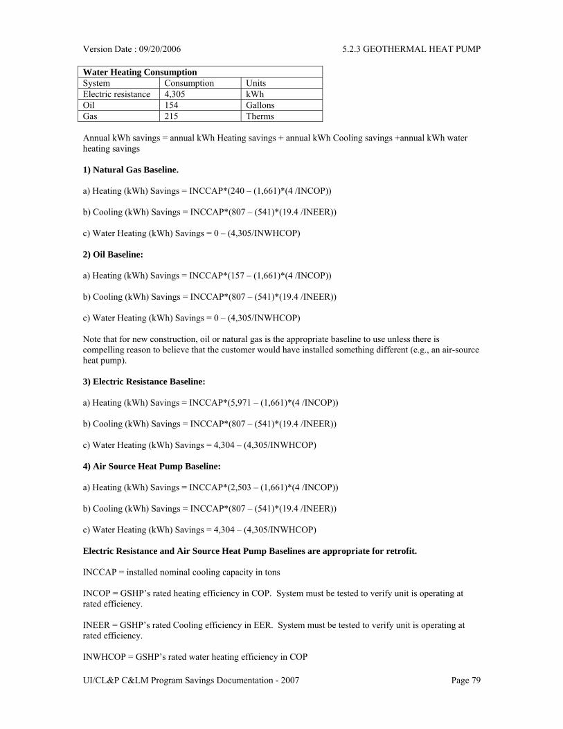
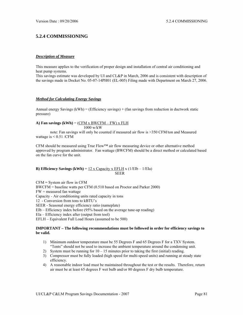
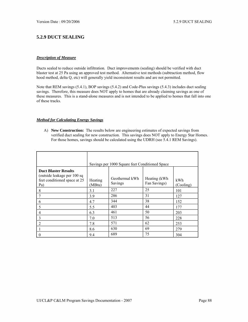
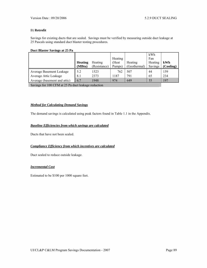
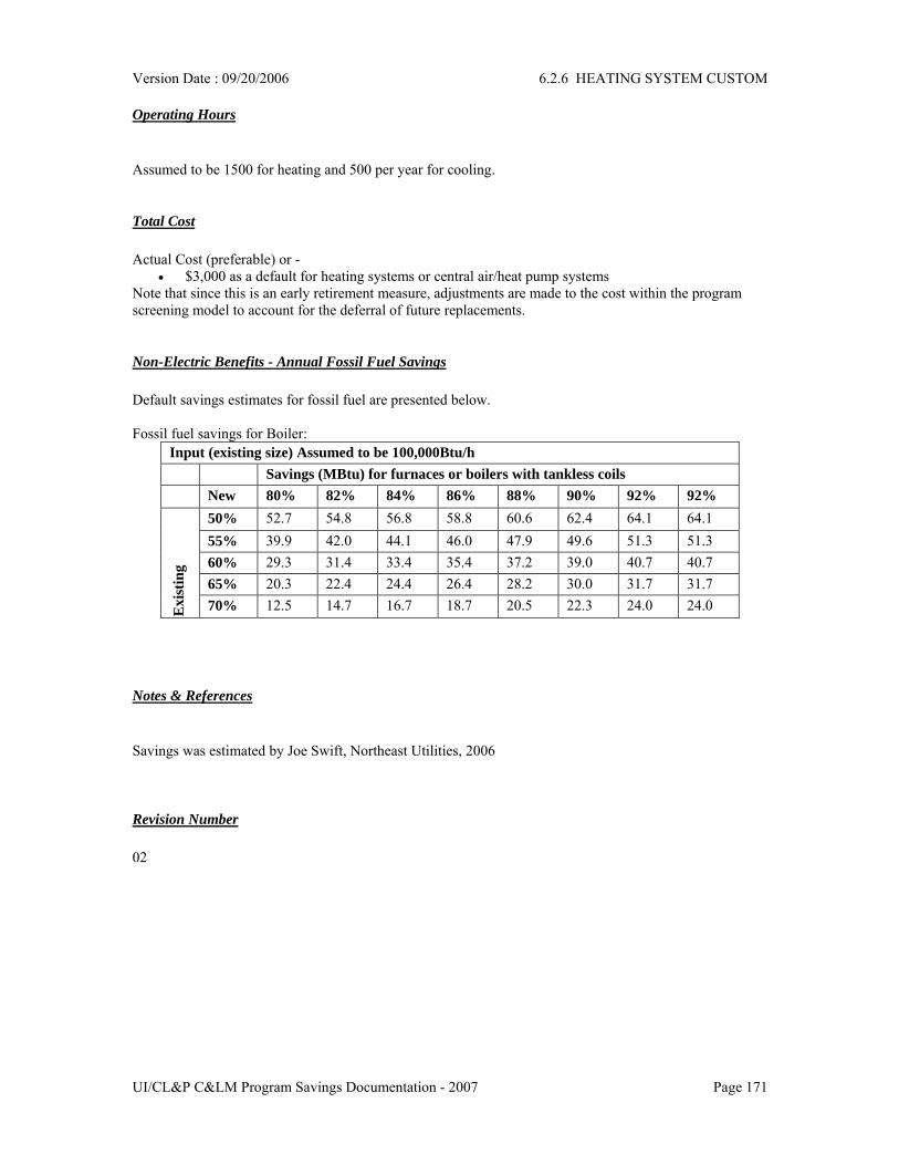
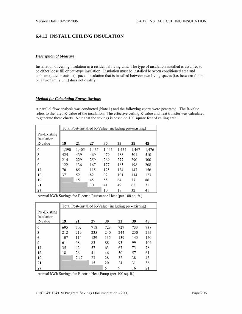
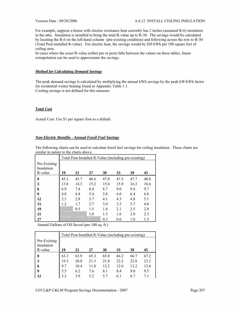
Version Date : 09/20/2006
UI/CL&P C&LM Program Savings Documentation - 2007 Page 3
Table of Contents INTRODUCTION.......................................................................................................................................... 6
UI/CL&P C&LM Program Savings Documentation - 2007 Page 6
INTRODUCTION
Version Date : 09/20/2006
UI/CL&P C&LM Program Savings Documentation - 2007 Page 7
1.1 BACKGROUND Introduction In 1999, the State Legislature created the Energy Conservation Management Board (ECMB) to guide and assist the State’s electric distribution companies in the development and implementation of cost-effective energy conservation programs and market transformation initiatives (CGS § 16-245m). The Connecticut Conservation and Load Management Fund (C&LM Fund) created by this legislation provides the financial support for ECMB-guided programs and initiatives. The Department of Public Utility Control (DPUC) is responsible for final approval of all C&LM Fund programs. The State’s energy conservation efforts, as administered by Connecticut Light & Power and United Illuminating, with guidance from the ECMB, focus on realizing the following primary objectives:
1. Advancing the Efficient Use of Energy C&LM programs are critical in reducing overall energy consumption and reducing load during periods of intense peak demand. These programs alleviate potential electricity shortages and reduce stress on transmission lines in the State, especially in southwestern Connecticut (SWCT).
2. Reduce Air Pollution and Negative Environmental Impacts Conservation programs produce environmental benefits by slowing the electricity demand growth rate, thereby avoiding emissions that would otherwise be produced by increased power generation activities. The Environmental Protection Agency regulates criteria air pollutants under the Clean Air Act’s National Ambient Air Quality Standards (NAAQSs). Connecticut’s conservation programs have significantly reduced two NAAQS criteria pollutants emitted in the process of generating electricity: sulfur dioxide and nitrogen oxides. Carbon dioxide and other “greenhouse gases”, such as methane, are also emitted during the process. Greenhouse gases have been cited as potential sources of global warming and climate change. With decreased power production resulting from declining electrical demand as a result of conservation efforts, C&LM programs reduce carbon dioxide emissions. C&LM programs, guided by the ECMB, support the State’s environmental initiatives to reduce these air pollutants as well as fine particulate emissions and ozone.
3. Promote Economic Development and Energy Security Energy efficiency programs generate considerable benefits for Connecticut customers. Conservation programs are tailored to meet the particular needs of all customer classes, thereby benefiting all State residents. Energy efficiency measures assist low-income customers in reducing their energy costs, which typically comprise a significant percentage of their household income. Other groups that benefit from energy conservation programs include educational institutions, manufacturers, non-profit organizations, residential customers and small businesses. Conservation programs made possible by the C&LM Fund lower operating costs and improve efficiency, which increases the productivity of manufacturing processes for small and large businesses. By reducing operating costs and enhancing productivity, Connecticut businesses remain competitive in the dynamic global economy, avoiding unnecessary outsourcing of jobs and services. The retention of Connecticut businesses enhances the perception among potential businesses and investors that Connecticut’s economy is healthy and productive. Information regarding Connecticut’s energy conservation programs is available at: The Connecticut Light and Power Company: www.cl-p.com The United Illuminating Company: www.uinet.com Conservation Program hot line (CL&P and UI): 1-877-WISE USE The Energy Conservation Management Board www.state.ct.us/dpuc/ecmb
Version Date : 09/20/2006 1.1 BACKGROUND
UI/CL&P C&LM Program Savings Documentation - 2007 Page 8
Purpose This manual provides detailed, comprehensive documentation of all claimed resource costs and savings corresponding to individual C&LM technologies. This project fulfills the Department’s requirement to develop a Technical Reference Manual (Docket NO. 03-11-01PH02, DPUC Review of CL&P and UI Conservation and Load Management Plan for Year 2004 – Phase II, July 28, 2004). CL&P and UI have worked together over the past several years to develop common assumptions regarding measured savings for all types of energy efficient measures. This manual is a compilation of those efforts. C&LM savings claims will be traceable through cross-references to this manual. The manual will be reviewed annually and updated to reflect changes in technology, baselines, measured savings, evaluation work, and impact factors. The C&LM savings calculations in this manual represent typical measures and prescriptive calculations used for those measures. In some cases, projects are more comprehensive or prescriptive measure calculations are not appropriate. To accurately calculate the savings related to these types of projects, more detailed spreadsheets or computer simulation models (DOE-2, Trace, HAP) must be used. Third-party engineering consultants are contracted to run all simulations and create many of these more detailed spreadsheets; all are reviewed for reasonableness. Organization C&LM measures in this manual are grouped by primary sector and reflect how programs and measures are organized within C&LM. Commercial and Industrial (C&I) measures are also categorized as either “Lost Opportunity” or “Retrofit”. The main sections of the manual are as follows:
• Introduction • Section 2: C&I Lost Opportunity • Section 3: C&I Retrofit • Section 4: Small Business • Section 5: Residential • Section 6: Low Income • Appendices
Savings Calculations Savings results presented in this manual (both electric and non-electric) are assumed to be the savings that would be measured at the point of use. Electric savings (both kWh and kW) are assumed to be the savings that would occur at the customer’s meter. Line losses are not included in the savings values presented here; their effects are captured within the screening model that the companies use to evaluate the benefits of conservation programs. In addition, the annual electric savings from measures has a specified load shape (i.e. the time of day at which savings occur). See Table 1.2 for load shapes for various end-use savings. The load shapes are used to properly assign the value of energy savings resulting from the implementation of C&LM measures to the corresponding time of day when those savings are realized. ` The value of demand savings for each measure takes into account the average run time on peak and the average power level that occurs at the time of the peak. For summer, the peak demand savings is defined to be the average peak savings from a measure that occurs during the “typical summer peak” which is defined as the two-hour window from 3:00 pm to 5:00 pm on the weekday with the highest heat index - the time period with the highest levels of discomfort as result of heat and humidity. For winter demand savings (for measures where this applies), the peak demand savings is defined to be the average peak savings from a measure that occurs during the “typical winter peak” which is defined as the two-hour window from 5:00 pm to 7:00 pm on the “coldest” winter weekday.
Version Date : 09/20/2006 1.1 BACKGROUND
UI/CL&P C&LM Program Savings Documentation - 2007 Page 9
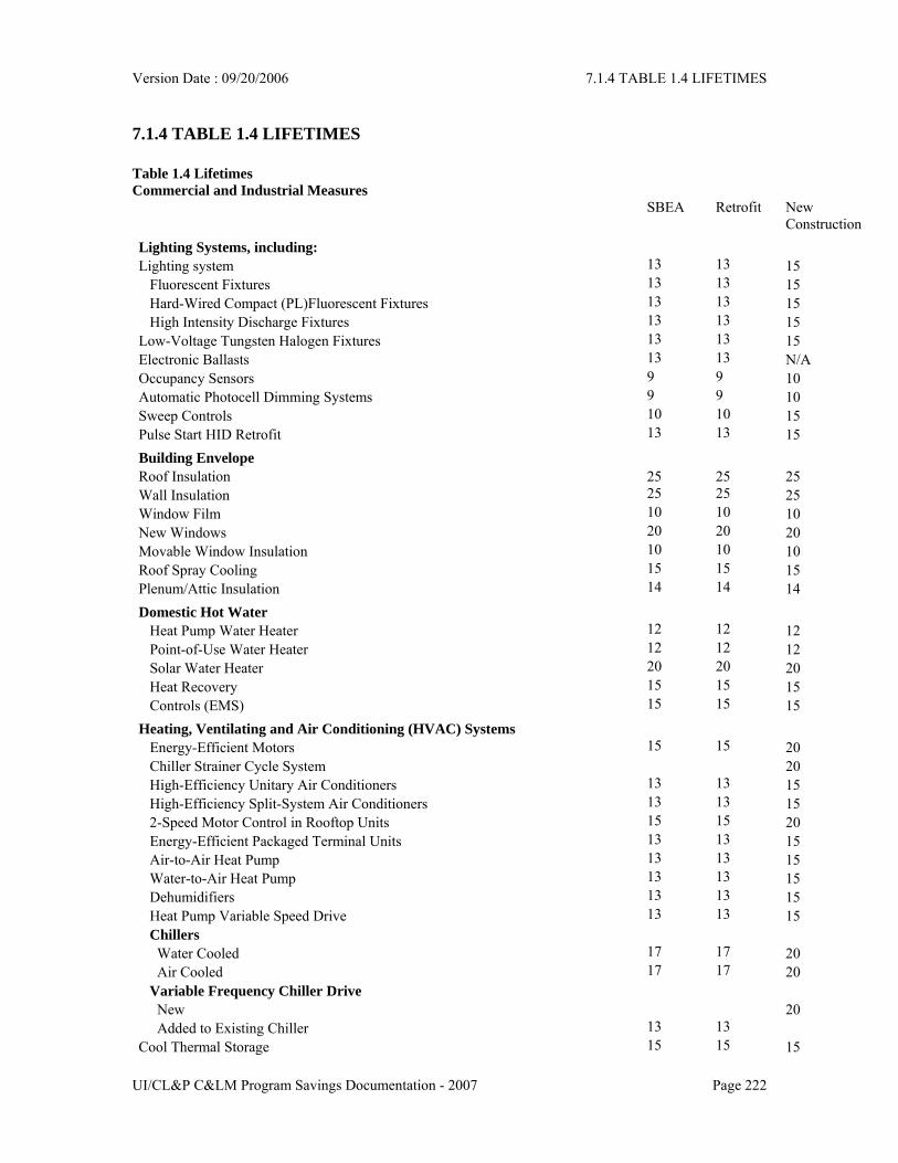
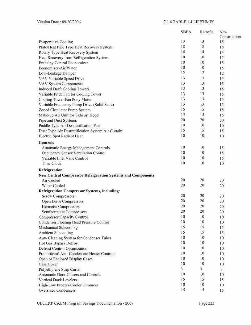
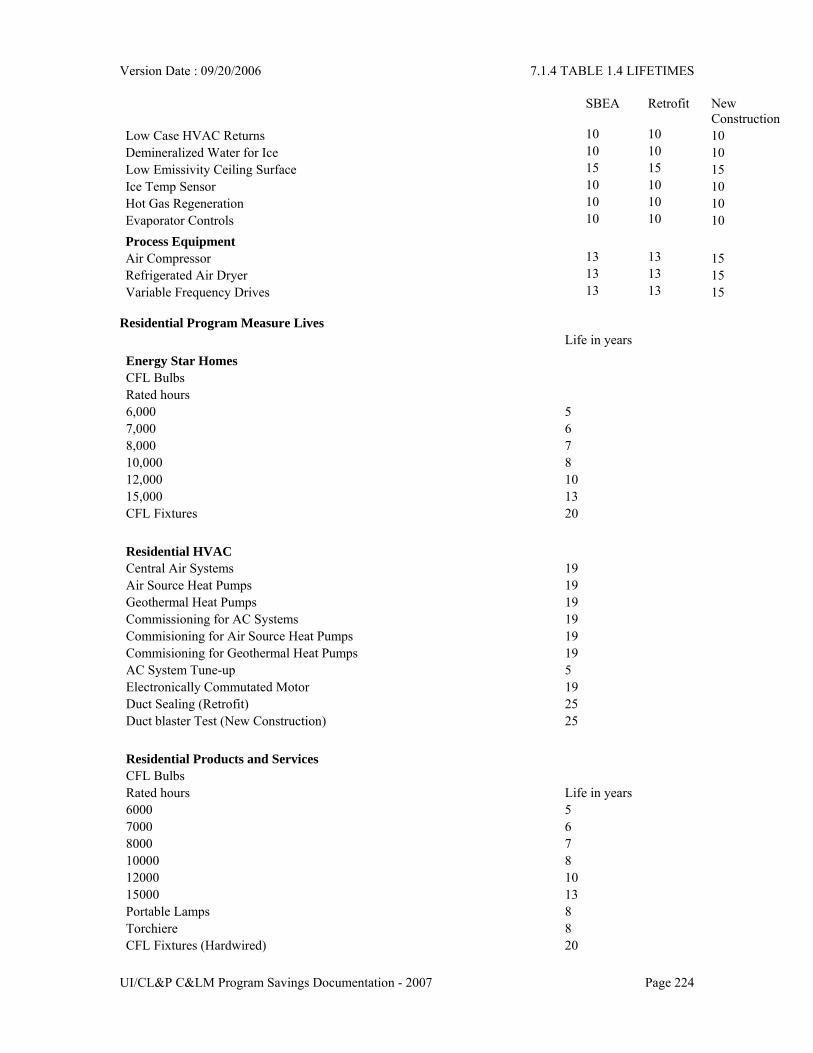
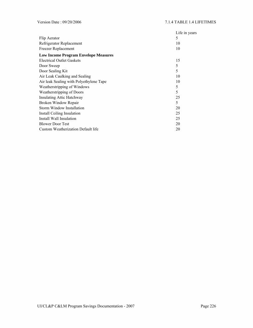
Peak demand savings can be calculated either on a measure-by-measure basis; or, on a default basis, coincidence factors can be used to calculate demand savings based on the annual savings and load shape of the measure. Coincidence factors are multiplied by the connected load savings of the measure in order to obtain the peak demand savings. See Table 1.1 for a list of default coincidence factors that are used to calculate the peak demand savings. ISO-NE uses a slightly different peak period in the summer for participants in its demand reduction programs. That period is 1:00 pm to 5:00 pm, and coincidence factors for that period are also shown in Table 1.1. In addition to electric benefits, some measures have non-electric benefits associated with them. Where appropriate, these benefits (or “impacts” since they can also be negative) are defined in this manual. Non-electric impacts may include quantifiable changes in fossil fuel consumption, water use, maintenance costs, productivity improvements, replacement costs, etc. Non-electric benefits are not included in the Electric System test; they are captured in the Total Resource Cost Test. The savings for the measures in this manual are calculated in two steps: (1) gross savings is calculated and (2) impact factors are applied to the gross savings to calculate the net (final) savings. Gross energy savings estimates (based on known technical parameters) represents the first step in calculating energy savings. Gross savings estimates are based on engineering algorithms or modeling that take into account technically important factors such as hours of use, differences in efficiency, differences in power consumption, etc. There are also some other factors beyond the engineering parameters that need to be considered when calculating the total impact of energy saving measures. For instance, market effects such as free-ridership, spillover or installation rate. The equation for net savings is as follows: Net Savings = Gross Savings x (1 + spillover – free-ridership) x Installation Rate In some cases, evaluation work may uncover differences between calculated savings and actual (metered) savings where those differences may not be (completely) attributable to the impact factors above. These differences may arise when the savings calculations do not accurately capture the real savings attributable to a measure. In addition to the impact factors above, savings differences can happen for a variety of reasons such as non-standard usage patterns or operating conditions. In these cases, overall net-to-gross ratios (realization rates) may be used in addition to (or instead of) the aforementioned impact factors to bring the observed savings values more in line with the original savings calculations. For instance, a billing analysis may show observed savings from a refrigerator removal program to be 60% of the gross (calculated) savings. In this case, the differences may be probably attributable to a combination of factors including refrigerators that were not being used, free-ridership, units being improperly used (e.g. the refrigerator door left open for long periods of time) or units that exhibited lower energy use because they were operating in cooler basement environments. In such a case, a 60% realization rate (adjustment) would be applied to the gross (calculated) energy savings to correct it. Realization rates can be applied to specific measures or across programs depending on their source. Since commercial and industrial (C&I) programs typically offer a wide range of diverse measures, defining specific impact factors for Commercial and Industrial (C&I) programs can be difficult, and therefore program specific realization rates are usually limited to C&I programs. Table 1.3 contains a list of program specific realization rates. These rates have been updated from 2006 based on recent studies. Realization rates are no longer included in the description of each individual measure. Other Changes from 2006 Measure lives are shown in Table 1.4 instead of in the individual measures. Energy Star transformers are now required to be installed in Ct, so its measure has been dropped from 2007.
Version Date : 09/20/2006 1.2 GLOSSARY
UI/CL&P C&LM Program Savings Documentation - 2007 Page 10
1.2 GLOSSARY The glossary provides definitions of the energy conservation terms used in this Technical Reference Manual. Note that some of these terms may have alternative or multiple definitions some of which may be outside the context of the manual. Only definitions pertaining to this manual are included in the glossary. Baseline Efficiency: C&LM program savings are calculated from this efficiency value. It represents the value of efficiency of the equipment that would have been installed without any influence from the program. Contrast compliance efficiency. Baseline Standard: The source or document that provides the Baseline Efficiency values, or a means to calculate these values. In many cases, the baseline efficiency is the minimum efficiency required by codes and standards, such as the Connecticut Energy Code. Coincident Demand: Demand of a measure that occurs at the same time as some other peak (building peak, system peak, etc). In the context of this document, coincident demand is a measure of demand savings that is coincident with electric system peak demand. Coincidence Factor: Coincidence factors represent the fraction of connected load expected to occur at the same time as a particular system peak period, on a diversified basis. Coincidence factors are normally expressed as a percent (of connected load). Also referred to as Diversity Factor. Compliance Efficiency: This efficiency value must be achieved in order to qualify for a C&LM program incentive. Contrast baseline efficiency. Compliance Standard: The source or document that provides the Compliance Efficiency values, or a means to calculate these values. In many cases the compliance efficiency is based on standards from recognized programs such as Energy Star. Connected Load: This is the maximum power required by the equipment, usually expressed as kW. Demand: The average electric power requirement (load) during a time period. Demand is measured in kW and the time period is usually one hour. If the time period is different than one hour, the time period is usually stated, such as “15-minute demand.” Demand can refer to an individual customer’s load or to the load of an entire electric system. See Peak Demand. Demand Savings: The difference in demand due to installation of an energy efficiency measure, usually expressed as kW and measured at the customer’s meter. For the purpose of this manual, demand savings is “coincident (with system peak) demand savings.” See Peak Demand Savings, Summer Demand Savings and Winter Demand Savings. Diversity Factor – See Coincidence Factor. Electric System (benefit-cost ratio) Test: A ratio used to assess the effectiveness of energy efficiency efforts on the electric system. The electric system test is defined as the present value of the avoided electric system costs (including energy, capacity, transmission and distribution) divided by the program related costs of achieving the savings. The electric system test is the primary evaluation tool used to screen measures and programs in Connecticut. Energy efficiency efforts are cost-effective if the benefit-cost ratio is greater than 1.0. End Use: Refers to a category of measures with similar load shapes. There are several different acceptable industry standards for defining end-use categories. For the purpose of this manual, end uses are cooling, heating, lighting, refrigeration, water heating, motors, process, and other.
Version Date : 09/20/2006 1.2 GLOSSARY
UI/CL&P C&LM Program Savings Documentation - 2007 Page 11
Equivalent Full Load Hours (EFLH): This is the number of hours per year that the equipment would need to draw power at its connected load rating in order to consume its estimated annual kWh. It is calculated as annual kWh/connected kW. EFLH is the same as operating hours for technologies such as light bulbs; EFLH is less than operating hours for technologies that operate at part load for some of the time, such as air conditioners and motors. Evaluation Study: A study that is used to assess the true impacts of a program including but not limited to: energy and demand savings, non-electric benefits, market effects, program performance, or program cost-effectiveness. Free-Rider: A program participant who would have installed or implemented an energy efficiency measure even in absence of program marketing or incentives. Free-ridership: The fraction (usually expressed as a percent) of gross program savings that would have occurred even in the absence of a C&LM program. Gross Savings: A saving estimate, calculated from objective technical factors. The gross savings do not include impact factors. High Efficiency: The efficiency of the energy-saving equipment installed because of a conservation program. High efficiency equipment uses less energy than standard equipment. Impact Evaluation: A study that assesses the energy, demand, nor non-electric benefits associated with energy efficiency measures or programs. Impact Factor: A number (usually expressed as a percent) used to adjust the gross savings in order to reflect the savings observed by an impact study. Examples of impact factors include free-ridership, spillover and installation rate. Installation Rate: The fraction of the recorded products that are installed. For example, some screw-in compact fluorescent lights are bought as spares, and may not be installed until another burns out. Load Factor: The average fractional load at which the equipment runs. It is calculated as average load/connected load. Load Shape: The time-of-use pattern of a customer’s energy consumption or measure. Load shape can be defined as hourly and/or seasonally (winter/summer). Lost Opportunity: Refers to the new installation of an enduring unit of equipment (in the case of new construction) or the replacement of an enduring unit of equipment at the end of its useful life. An enduring unit of equipment is one that would normally be maintained, not replaced, until the end of its life. Contrast “retrofit” Market Effect: A change in the behavior of a market because of conservation efforts. “Market Effect savings” is the savings that results changes in market behaviors. MBtu: Millions of Btu. Measure: A product (a piece of equipment) or a process that is designed to provide energy or demand savings. Measure can also refer to a service or a practice that provides savings. Measure Cost: For new construction or measures that are installed at their natural time of replacement (replace upon burn-out), measure cost is defined as the incremental cost of upgrading to high efficiency. For retrofit measures, measure cost is defined as the full cost of the measure. Measure cost refers to the true cost of the measure regardless of whether an incentive was paid for that measure.
Version Date : 09/20/2006 1.2 GLOSSARY
UI/CL&P C&LM Program Savings Documentation - 2007 Page 12
Measure lifetimes: This is the average number of years (or hours) that a group of new high efficiency equipment will continue to produce energy savings or the average number of years that a service or practice will provide savings. Lifetimes are generally based on experience or studies. Measure type: Refers to a category of similar measures. There are several different acceptable industry standards for defining end-use categories. For the purpose of this manual, end use categories are Lighting, HVAC, Motors, VFD (variable frequency drives), Refrigeration, Products & Services, Envelope, Renewable, and Other. Net Savings: The final value of savings that is attributable to a program or measure. Net savings differs from “gross savings” because it includes adjustments from impact factors such as free-ridership or spillover. Net savings is sometimes referred to as “verified savings” or “final savings.” Net-to-gross: The ratio of net savings to the gross savings (for a measure or program). Net-to-gross is usually expressed as a percent. Non-electric benefits: Quantifiable benefits (beyond electric savings) that are the result of the installation of a measure. Fossil fuel, water and maintenance are examples of non-electric benefits. Non-electric benefits can be negative (i.e. increased maintenance or increased fossil fuel usage which results from a measure) and therefore are sometimes referred to as non-electric impacts. Non-Participant: A customer who is eligible to participate in a program, but does not. A non-participant may install a measure because of a program, but the installation of the measure is not through regular program channels; as a result, their actions are normally only detected through evaluations (see spillover). Operating Hours: The annual amount of time, in hours, that the equipment is expected to operate. Contrast Equivalent Full Load Hours. Participant: A customer who installs a measure through regular program channels and receives any benefit (i.e. incentive) that is available through the program because of his participation. Free-riders are a subset of this group. Peak Demand: The highest demand. Peak Demand Savings: The kW demand reduction that occurs in the peak period. See also Coincidence Factor, Demand Savings. Peak Factor: Multipliers that are used to calculate peak reductions for measures based on the end use of the measure and the annual electric energy savings from the measure. The units for peak factors are kW/kWh. Realization of Savings: The ratio of actual measure savings to gross measure savings (sometimes referred to as the “realization rate”). This ratio takes into account impact factors that can influence the actual savings of a program such as spillover, free-ridership, etc. Retrofit: The replacement of a piece of equipment or device before the end of its useful or planned life for the purpose of achieving energy savings. “Retrofit” measures are sometimes referred to as “early retirement” when the removal of the old equipment is aggressively pursued. Sector: A system for grouping customers with similar characteristics. For the purpose of this manual, the sectors are Commercial and Industrial (C&I), Small Business, Residential, and Low Income. Spillover: Savings attributable to the program, but additional to the gross (tracked savings) of a program. Spillover include the effects of : (a) participants in the program who install additional energy efficient measures outside of the program as a result of hearing about the program; or (b) non-participants who install or influence the installation of energy efficient measures as a result of being aware of the program.
Version Date : 09/20/2006 1.2 GLOSSARY
UI/CL&P C&LM Program Savings Documentation - 2007 Page 13
Summer Demand Savings: Refers to average demand savings that occurs during the summer system peak. See summer system peak. Summer System Peak: Defined as the average demand of all the 3:00 pm to 5:00 pm time periods on the non-holiday weekdays during June, July and August. This value is used in determining the effect on peak demand savings of individual measures participating in the conservation programs. Summer System Peak (ISO-NE): Defined as the average demand of all the 1:00 pm to 5:00 pm time periods on the non-holiday weekdays during June, July and August. ISO-NE uses this value in determining credits under its demand reduction programs. Summer System Peak (Utility Extreme): Defined as the historical time period when the Connecticut electric utilities observe their highest load. During the past 10 years, this has been from 3:00 pm to 5:00 pm on one of the hottest weekdays of the year. Total Resource (Benefit/Cost) Test: A test used to assess the net benefit of energy efficiency resources to society. The total resource test is different from the electric system test in that the total resource benefit consists of the avoided costs of all conserved energy (electric and other fuels) plus other non-energy resource impacts that may have occurred because of efficiency efforts such as reduced maintenance or higher productivity. The cost for the total resource benefit consists of all program-related costs and any costs incurred by the customer related to the installation of measures. Winter Demand Savings: Refers to average demand savings that occurs during the winter system peak. See winter system peak. Winter system peak: Defined as the time period from 5:00 to 7:00 pm on the coldest weekday(s) of the year.
Version Date : 09/20/2006 1.2 GLOSSARY
UI/CL&P C&LM Program Savings Documentation - 2007 Page 14
C&I LOST OPPORTUNITY
Version Date : 09/20/2006 2.1.1 STANDARD LIGHTING
UI/CL&P C&LM Program Savings Documentation - 2007 Page 15
2.1.1 STANDARD LIGHTING
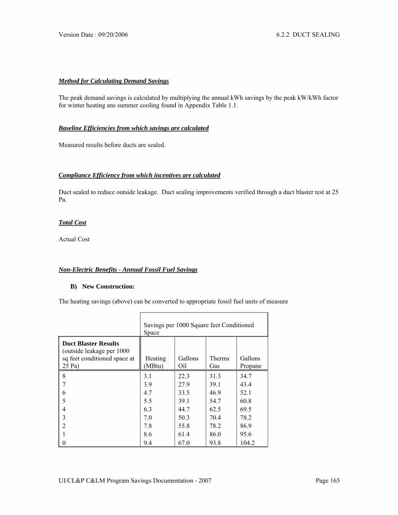
Description of Measure Encourage and reward lighting power levels that exceed the standards.
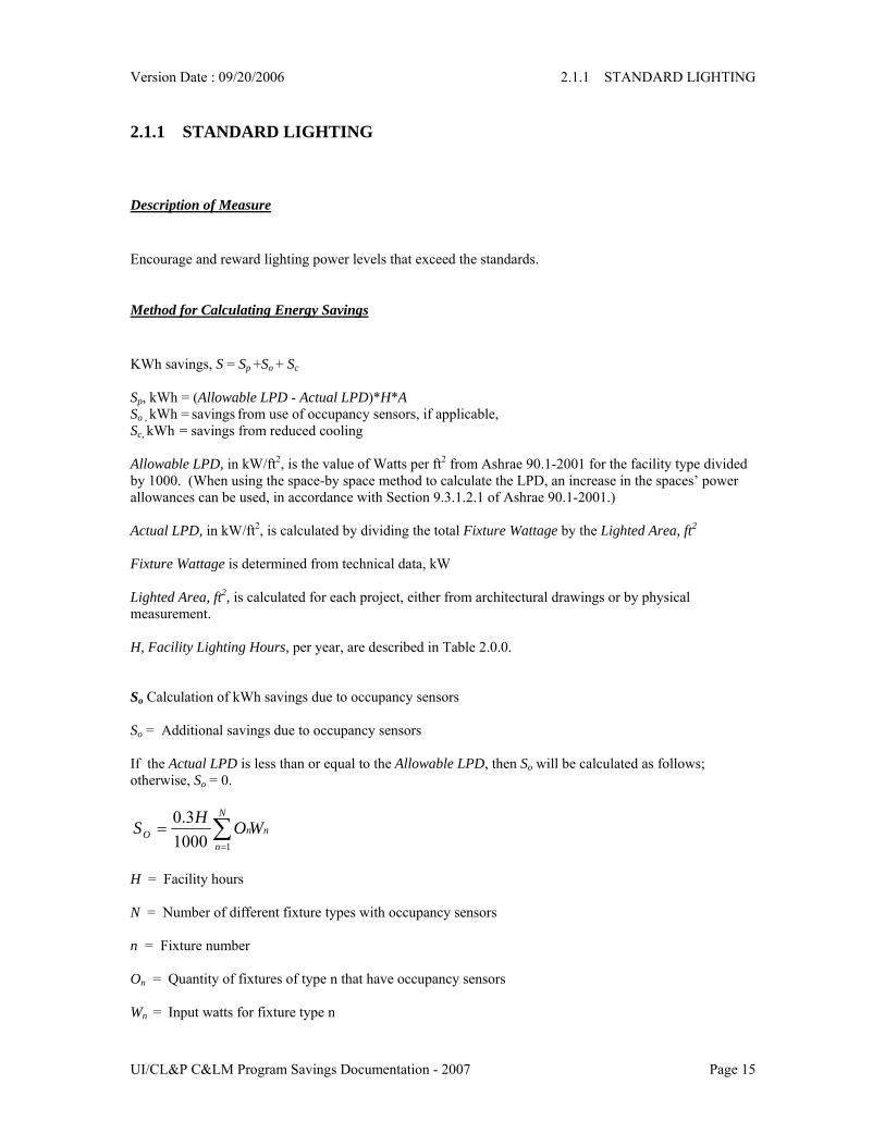
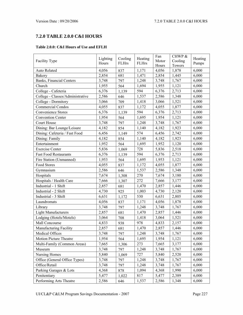
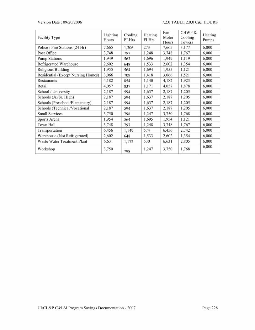
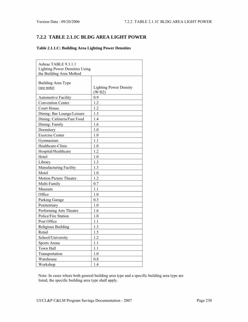
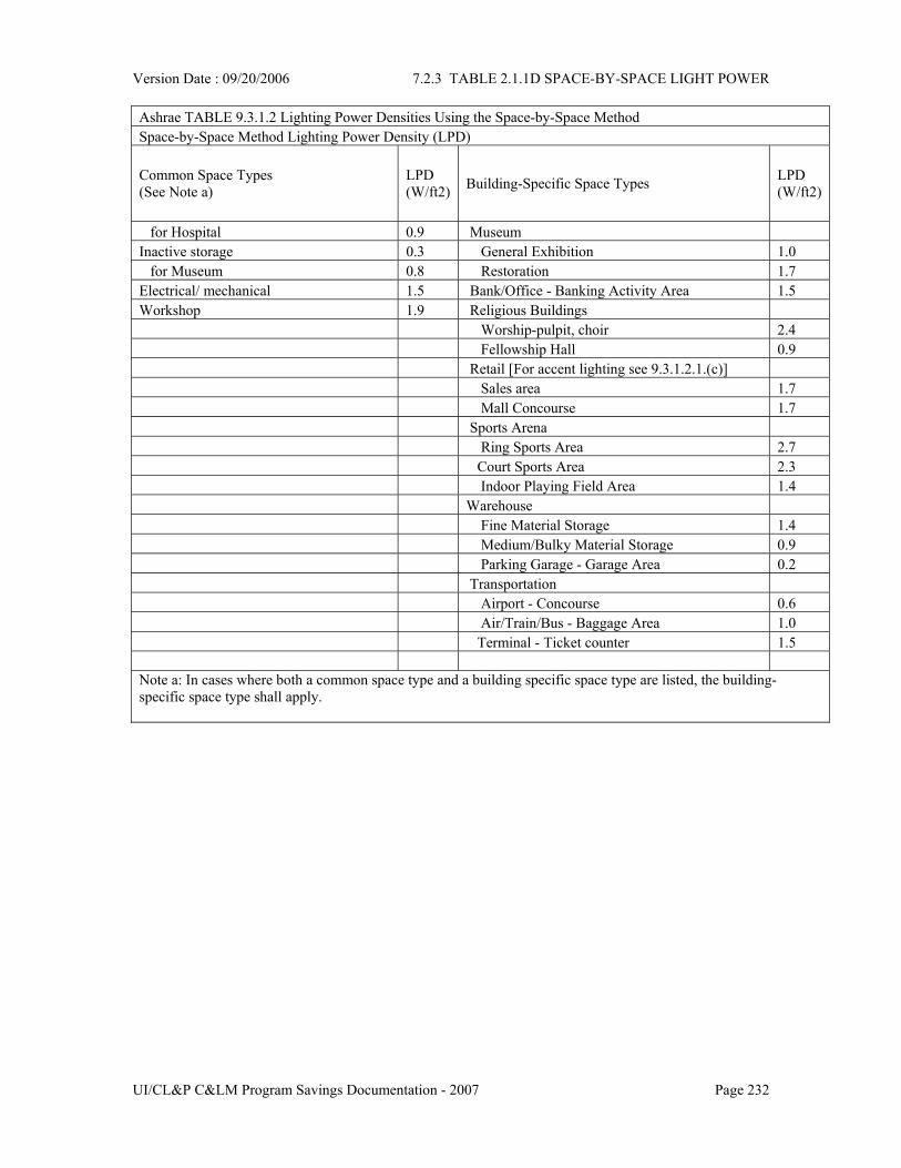
Method for Calculating Energy Savings KWh savings, S = Sp +So + Sc Sp, kWh = (Allowable LPD - Actual LPD)*H*A So , kWh = savings from use of occupancy sensors, if applicable, Sc, kWh = savings from reduced cooling Allowable LPD, in kW/ft2, is the value of Watts per ft2 from Ashrae 90.1-2001 for the facility type divided by 1000. (When using the space-by space method to calculate the LPD, an increase in the spaces’ power allowances can be used, in accordance with Section 9.3.1.2.1 of Ashrae 90.1-2001.) Actual LPD, in kW/ft2, is calculated by dividing the total Fixture Wattage by the Lighted Area, ft2 Fixture Wattage is determined from technical data, kW Lighted Area, ft2, is calculated for each project, either from architectural drawings or by physical measurement. H, Facility Lighting Hours, per year, are described in Table 2.0.0. So Calculation of kWh savings due to occupancy sensors So = Additional savings due to occupancy sensors If the Actual LPD is less than or equal to the Allowable LPD, then So will be calculated as follows; otherwise, So = 0.
n
N
nnO WOHS ∑
=
=11000
3.0
H = Facility hours N = Number of different fixture types with occupancy sensors n = Fixture number On = Quantity of fixtures of type n that have occupancy sensors Wn = Input watts for fixture type n
Version Date : 09/20/2006 2.1.1 STANDARD LIGHTING
UI/CL&P C&LM Program Savings Documentation - 2007 Page 16
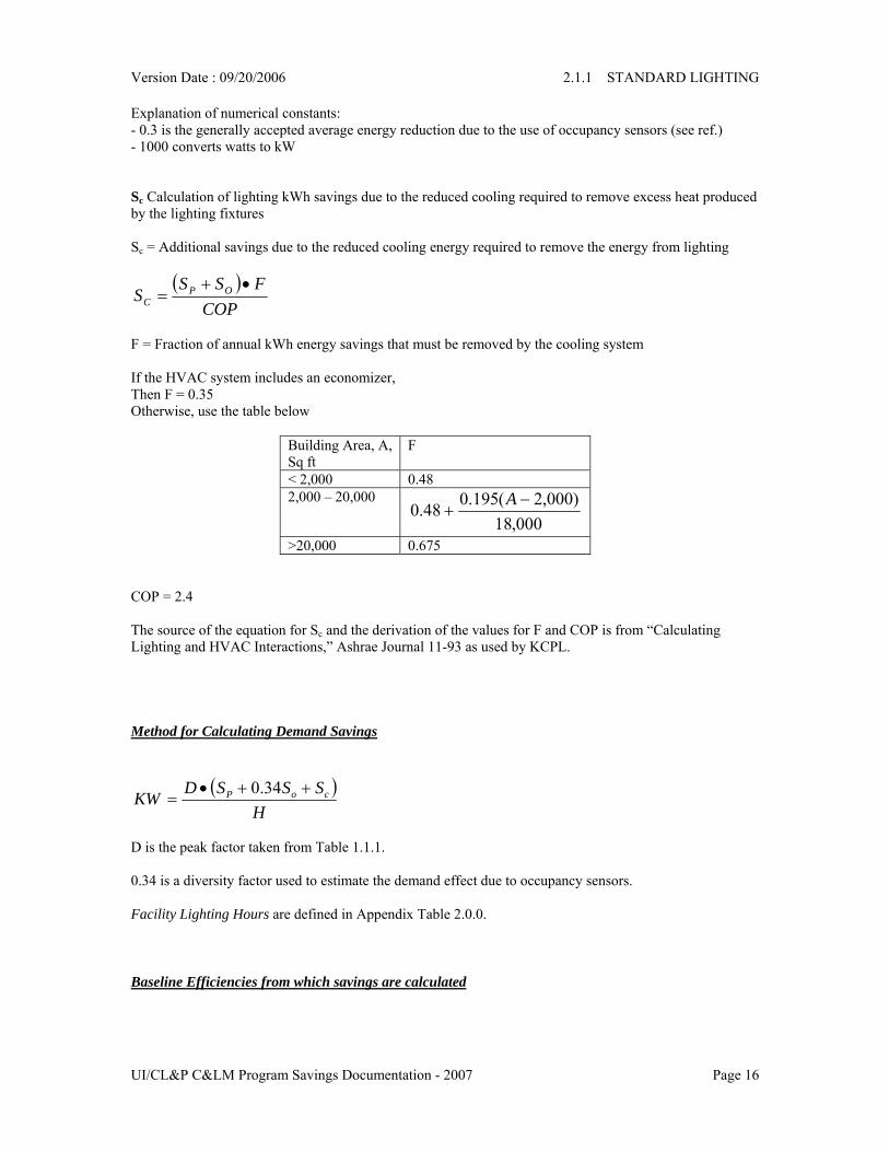
Explanation of numerical constants: - 0.3 is the generally accepted average energy reduction due to the use of occupancy sensors (see ref.) - 1000 converts watts to kW Sc Calculation of lighting kWh savings due to the reduced cooling required to remove excess heat produced by the lighting fixtures Sc = Additional savings due to the reduced cooling energy required to remove the energy from lighting
( )COP
FSSS OP
C•+
=
F = Fraction of annual kWh energy savings that must be removed by the cooling system If the HVAC system includes an economizer, Then F = 0.35 Otherwise, use the table below
Building Area, A, Sq ft
F
< 2,000 0.48 2,000 – 20,000
000,18)000,2(195.048.0 −
+A
>20,000 0.675
COP = 2.4 The source of the equation for Sc and the derivation of the values for F and COP is from “Calculating Lighting and HVAC Interactions,” Ashrae Journal 11-93 as used by KCPL.
Method for Calculating Demand Savings
( )H
SSSDKW coP ++•=
34.0
D is the peak factor taken from Table 1.1.1. 0.34 is a diversity factor used to estimate the demand effect due to occupancy sensors. Facility Lighting Hours are defined in Appendix Table 2.0.0.
Baseline Efficiencies from which savings are calculated
Version Date : 09/20/2006 2.1.1 STANDARD LIGHTING
UI/CL&P C&LM Program Savings Documentation - 2007 Page 17
The baseline allowable Lighting Power Densities are those shown in Ashrae 90.1-2001 Tables 9.3.1.1 and 9.3.1.2, as modified by Addenda (g) and (ag). These tables are reproduced in the Appendix as Tables 2.1.1.C and 2.1.1.D, respectively.
Compliance Efficiency from which incentives are calculated 0.05 W/ft2 below the baseline LPD
Operating Hours Default Facility Lighting Hours are taken from Table 2.0.0.
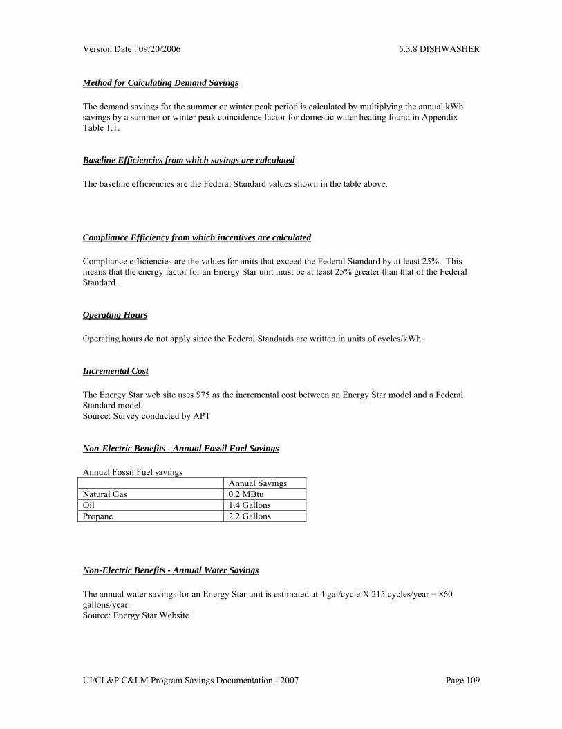
Non-Electric Benefits - Annual Fossil Fuel Savings Space heating increase from reduced lighting load. Annual Fossil fuel Savings = -0.00079 MBTU’s per annual kWh saved. Based on August 22, 2003 Memorandum from Optimal energy, Inc.
Non-Electric Benefits - Annual O&M Cost Adjustments O&M savings due to the reduction of lighting hours from installation of occupancy sensors. Annual O&M Savings = $0.014917 per annual kWh saved from the installation of occupancy sensors. Based on August 22, 2003 Memorandum from Optimal energy, Inc.
Notes & References Occupancy sensor savings reference: 1. D. Maniccia B. Von Neida, and A. Tweed. An analysis of the energy and cost savings potential of occupancy sensors for commercial lighting systems Illuminating Engineering Society of North America 2000 Annual Conference: Proceedings. IESNA: New York, NY. Pp. 433-459. 2. RLW Study “2005 Coincidence Factor Study With 1-5 Summer Peak Window”, 7-20-06.
Revision Number 12
Version Date : 09/20/2006 2.2.1 COOLING - CHILLERS
UI/CL&P C&LM Program Savings Documentation - 2007 Page 18
2.2.1 COOLING - CHILLERS
Description of Measure This measure encourages the installation of efficient water-cooled and air-cooled water chilling packages (chillers). Chillers must use an environmentally friendly refrigerant in order to qualify for the program.
Method for Calculating Energy Savings Energy savings are custom-calculated for each chiller installation based on the specific equipment, operational staging, operating profile, and load profile. Equipment Each chiller plant is characterized by its:
• Number of chillers, • Sizes, in tons (the chillers may be of different sizes), • Type, which may be:
o Centrifugal, R123 refrigerant, R134a refrigerant
o Water-cooled screw and scroll, or o Air-cooled
• Speed, constant or variable • Auxiliary equipment
o Chilled water pumps o Cooling tower pumps o Cooling tower fans o Other
Operational Staging If more than one chiller is used, their operational relationship can be defined. When the load is high enough to permit two chillers to operate, they can be designated to operate together at the same loading, or, alternatively, either one can be operated at full output while the other follows the cooling load profile. Operating Profile The customer’s cooling load profile, for each of 12 months, is characterized by:
• On-peak occupied hours the chiller is operated each week, • Off-peak occupied hours the chiller is operated each week, • On-peak un-occupied hours the chiller is operated each week, • Off-peak un-occupied hours the chiller is operated each week.
Load Profile The customer’s load profile is estimated by determining the load at the peak outdoor conditions and the load at the minimum conditions. For systems with an air-side or water-side economizer, the minimum conditions are those just above the set point of the economizer. If the customer’s load profile is not known,
Version Date : 09/20/2006 2.2.1 COOLING - CHILLERS
UI/CL&P C&LM Program Savings Documentation - 2007 Page 19
a default load profile will be developed; in this case it is also necessary to determine the value of any process loads. Savings Calculation With the above information, a calculation is made for each time period of the year based on the appropriate temperature bin data. The calculation is performed once for the chillers meeting the baseline efficiencies and again for the proposed chillers, and the difference determines the kWh and the kW savings for each period. These are summed to yield the total savings.
Method for Calculating Demand Savings The demand savings calculation is described in the previous paragraph.
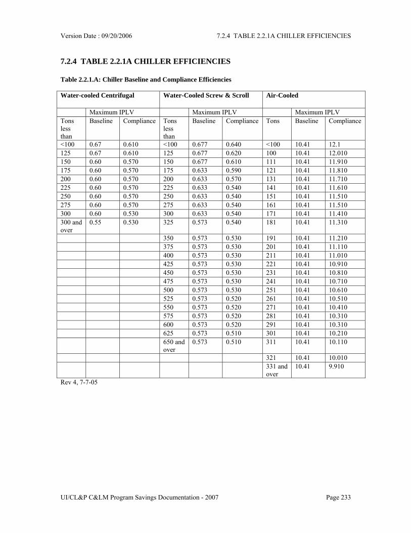
Baseline Efficiencies from which savings are calculated The baseline efficiencies are those required by the Ct Building Code. These efficiencies are shown in Table 2.2.1.A in the Appendix.
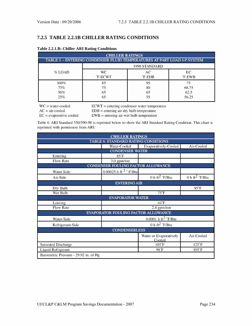
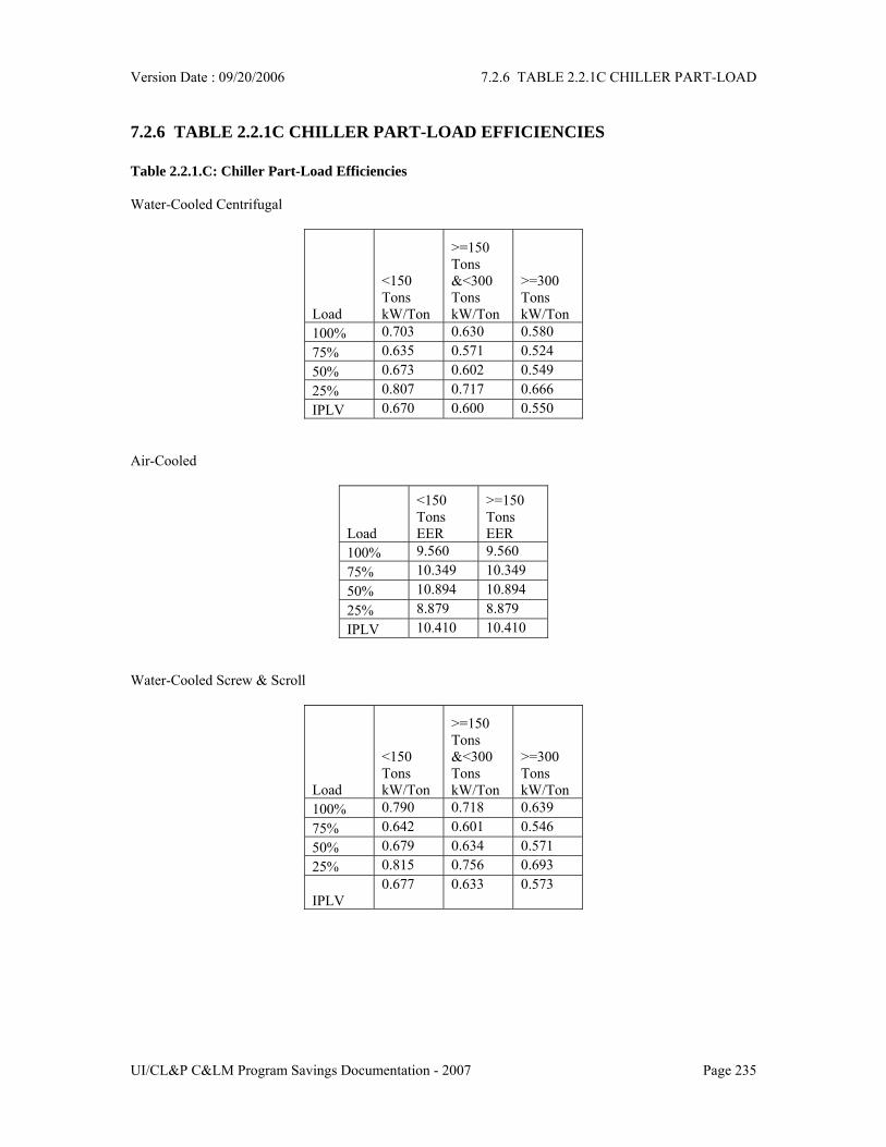
Compliance Efficiency from which incentives are calculated The chiller rating at ARI conditions must meet a minimum efficiency to qualify for an incentive. The minimum is set at an efficiency somewhat better than what Ashrae 90.1 requires. These minimum efficiency levels for the various sizes and types of chillers are shown in Table 2.2.1.A in the Appendix. The ARI conditions are shown in Table 2.2.1.B in the Appendix The part-load efficiencies that are used to compute the savings are shown in Table 2.2.1.C. These values are not part of Ashrae 90.1-2001. They are based on reported part-load efficiencies of chillers.
Operating Hours A single value for operating hours is not used. As described above, custom hourly calculations are made for each customer.
Non-Electric Benefits - Annual Fossil Fuel Savings The realization of savings is based on program. Refer to table 7.1.3
Revision Number 09
Version Date : 09/20/2006 2.2.2 COOLING - UNITARY AC & HEAT PUMPS
UI/CL&P C&LM Program Savings Documentation - 2007 Page 20
2.2.2 COOLING - UNITARY AC & HEAT PUMPS
Description of Measure This measure encourages the installation of efficient Direct-Expansion (DX) cooling systems for C&I customers.
Method for Calculating Energy Savings Cooling (A/C units and Air Source Heat Pumps)
EFLHh = Refer to Table 2.0.0 Cap = Unit’s rated cooling capacity in Btu/h EERi = Installed unit’s rated energy efficiency ratio EERb = Baseline energy efficiency ratio (see table below) (Note: SEERp and SEERb are used for units < 5.4 tons) HSPFb = Baseline Heating seasonal performance factor, watt hours per MBtu heat input HSPFi = installed Heating seasonal performance factor EFLHc = equivalent full load hours cooling EFLHh = equivalent full load hours heating 1000 = converts Wh to kWh Ratio 13900/12000 = ratio of heat produced in the heating mode divided by cooling produced in the cooling mode.
Method for Calculating Demand Savings Summer kW savings = D* Cap * (1/(EERb)-1/(EERi)) /1000 Winter kW savings = 0, Cooling only units have no winter demand savings since they do not operate during the winter. Air source heat pumps have no winter demand savings because they use resistance back up at low outside air temperatures.
Version Date : 09/20/2006 2.2.2 COOLING - UNITARY AC & HEAT PUMPS
UI/CL&P C&LM Program Savings Documentation - 2007 Page 21
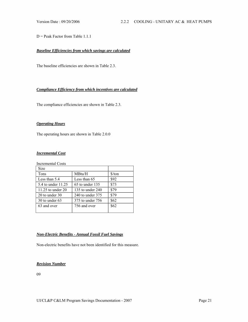
D = Peak Factor from Table 1.1.1
Baseline Efficiencies from which savings are calculated The baseline efficiencies are shown in Table 2.3.
Compliance Efficiency from which incentives are calculated The compliance efficiencies are shown in Table 2.3.
Operating Hours The operating hours are shown in Table 2.0.0
Incremental Cost Incremental Costs Size Tons MBtu/H $/ton Less than 5.4 Less than 65 $92 5.4 to under 11.25 65 to under 135 $73 11.25 to under 20 135 to under 240 $79 20 to under 30 240 to under 375 $79 30 to under 63 375 to under 756 $62 63 and over 756 and over $62
Non-Electric Benefits - Annual Fossil Fuel Savings Non-electric benefits have not been identified for this measure.
Revision Number 09
Version Date : 09/20/2006 2.2.3 COOLING - WATER AND GROUND SOURCE HP
UI/CL&P C&LM Program Savings Documentation - 2007 Page 22
2.2.3 COOLING - WATER AND GROUND SOURCE HP
Description of Measure The measure is to encourage efficiency upgrades of water-to-air heat pump units at the time of their replacement or new construction.
Method for Calculating Energy Savings Cooling Annual cooling kWh savings = Cap * (1/(EERb)-1/(EERi)) * EFLHc/1000 EFLHc = refer to Table 2.0.0 Heating
Annual heating kWh savings = H
IB
EFLHCOPCOP
Cap ∗∗⎟⎟⎠
⎞⎜⎜⎝
⎛−∗∗
3413111
000,12900,13
EFLHh = refer to Table 2.0.0 Cap = Unit’s rated cooling capacity in Btu/h EERi = Installed unit’s rated energy efficiency ratio EERb = Baseline energy efficiency ratio (see table below) COPb = Baseline Heating Coefficient of performance COPi = Installed Heating Coefficient of performance EFLHc = equivalent full load hours cooling EFLHh = equivalent full load hours heating 3413 = converts Btu/h to kW Ratio 13900/12000 = ratio of heat produced in the heating mode divided by cooling produced in the cooling mode.
Version Date : 09/20/2006 2.2.3 COOLING - WATER AND GROUND SOURCE HP
UI/CL&P C&LM Program Savings Documentation - 2007 Page 23
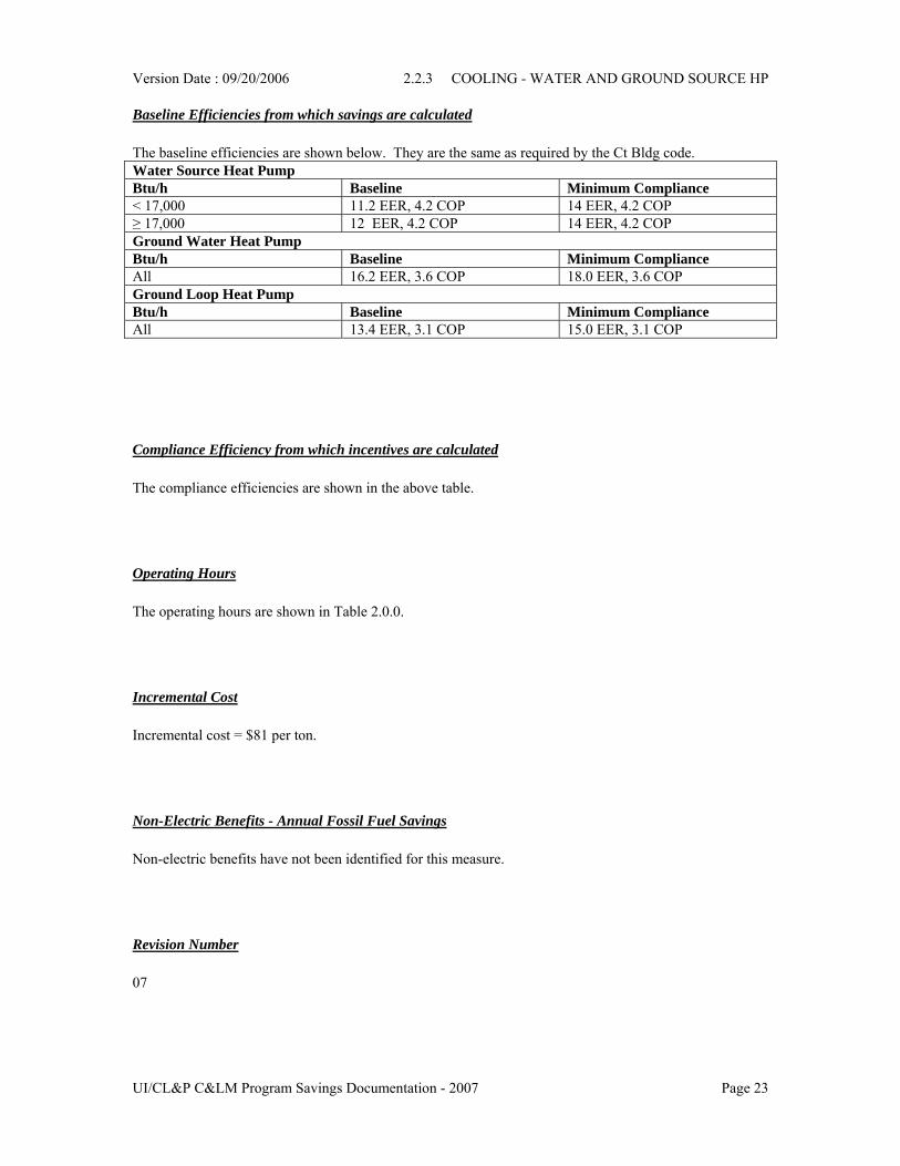
Baseline Efficiencies from which savings are calculated The baseline efficiencies are shown below. They are the same as required by the Ct Bldg code. Water Source Heat Pump Btu/h Baseline Minimum Compliance < 17,000 11.2 EER, 4.2 COP 14 EER, 4.2 COP ≥ 17,000 12 EER, 4.2 COP 14 EER, 4.2 COP Ground Water Heat Pump Btu/h Baseline Minimum Compliance All 16.2 EER, 3.6 COP 18.0 EER, 3.6 COP Ground Loop Heat Pump Btu/h Baseline Minimum Compliance All 13.4 EER, 3.1 COP 15.0 EER, 3.1 COP
Compliance Efficiency from which incentives are calculated The compliance efficiencies are shown in the above table.
Operating Hours The operating hours are shown in Table 2.0.0.
Incremental Cost Incremental cost = $81 per ton.
Non-Electric Benefits - Annual Fossil Fuel Savings Non-electric benefits have not been identified for this measure.
Revision Number 07
Version Date : 09/20/2006 2.2.4 COOLING - DUAL ENTHALPY CONTROLS
UI/CL&P C&LM Program Savings Documentation - 2007 Page 24
2.2.4 COOLING - DUAL ENTHALPY CONTROLS
Description of Measure The measure is to upgrade the outside-air dry-bulb economizer to a dual enthalpy economizer. The system will continuously monitor the enthalpy of both the outside air and return air. The system will control the system dampers adjust the outside quantity based on the two readings.
Method for Calculating Energy Savings Annual cooling kWh savings = Tons * 276 kWh / Ton Tons = Unit’s rated cooling capacity in Tons The 276 kWh / ton average savings is based on DOE-2 simulation results broad cross section of building types and sizes.
Method for Calculating Demand Savings Summer kW savings = 0 Demand savings are zero since the measure reduces energy when outside temperatures are low.
Baseline Efficiencies from which savings are calculated HVAC operating with fixed dry-bulb economizer.
Operating Hours The operating hours are not used in the calculation.
Incremental Cost $250 per unit controlled
Version Date : 09/20/2006 2.2.4 COOLING - DUAL ENTHALPY CONTROLS
UI/CL&P C&LM Program Savings Documentation - 2007 Page 25
Non-Electric Benefits - Annual Fossil Fuel Savings Non-electric benefits have not been identified for this measure.
Revision Number 02
Version Date : 09/20/2006 2.2.5 VENTILATION CO2 CONTROLS
UI/CL&P C&LM Program Savings Documentation - 2007 Page 26
2.2.5 VENTILATION CO2 CONTROLS
Description of Measure The measure is to upgrade CO2 control of outside air to an air handling system. The proposed systems monitor the CO2 in the spaces or return air and reduce the outside air when possible to save energy without affecting the indoor air quality.
Method for Calculating Energy Savings Cooling The electrical savings are custom-calculated for all projects. Savings are based on hours of operation, return air dry bulb temperature, return air enthalpy, system total air flow, percent outside air, estimated average outside air reduction, and cooling efficiency. Savings are estimated based using a temperature BIN spreadsheet that calculates the difference in outside air enthalpy and return air enthalpy from the reduction in outside air.
Method for Calculating Demand Savings Summer demand savings are calculated based on the top temperature BINs used in the spreadsheet.
Baseline Efficiencies from which savings are calculated No ventilation control.
Operating Hours Operating hours are site specific.
Incremental Cost $750 to $1,500 per unit controlled.
Version Date : 09/20/2006 2.2.5 VENTILATION CO2 CONTROLS
UI/CL&P C&LM Program Savings Documentation - 2007 Page 27
Non-Electric Benefits - Annual Fossil Fuel Savings The fossil fuel savings are custom-calculated for all projects. Savings are based on return air dry bulb temperature, return air enthalpy, system total air flow, percent outside air, estimated average outside air reduction, and boiler efficiency. Savings are estimated based using a temperature BIN spreadsheet that calculates the difference in outside air enthalpy and return air enthalpy from the reduction in outside air.
Revision Number 03
Version Date : 09/20/2006 2.3.1 C&I LO MOTORS
UI/CL&P C&LM Program Savings Documentation - 2007 Page 28
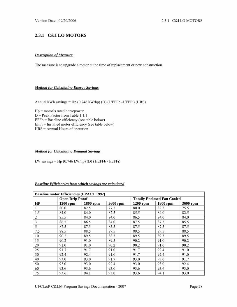
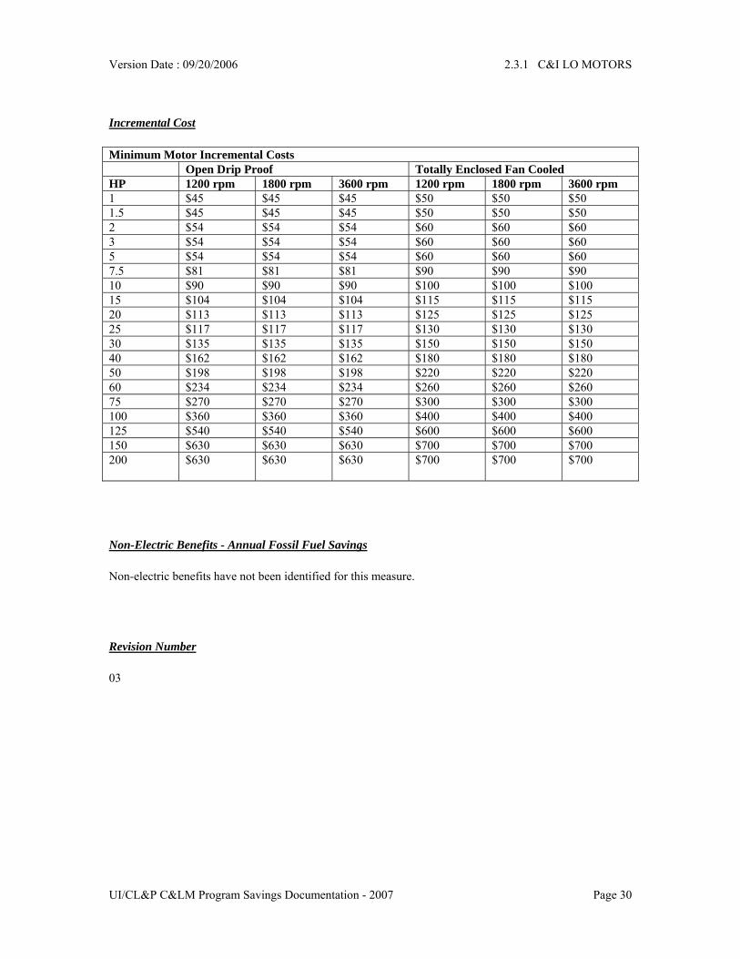
2.3.1 C&I LO MOTORS
Description of Measure The measure is to upgrade a motor at the time of replacement or new construction.
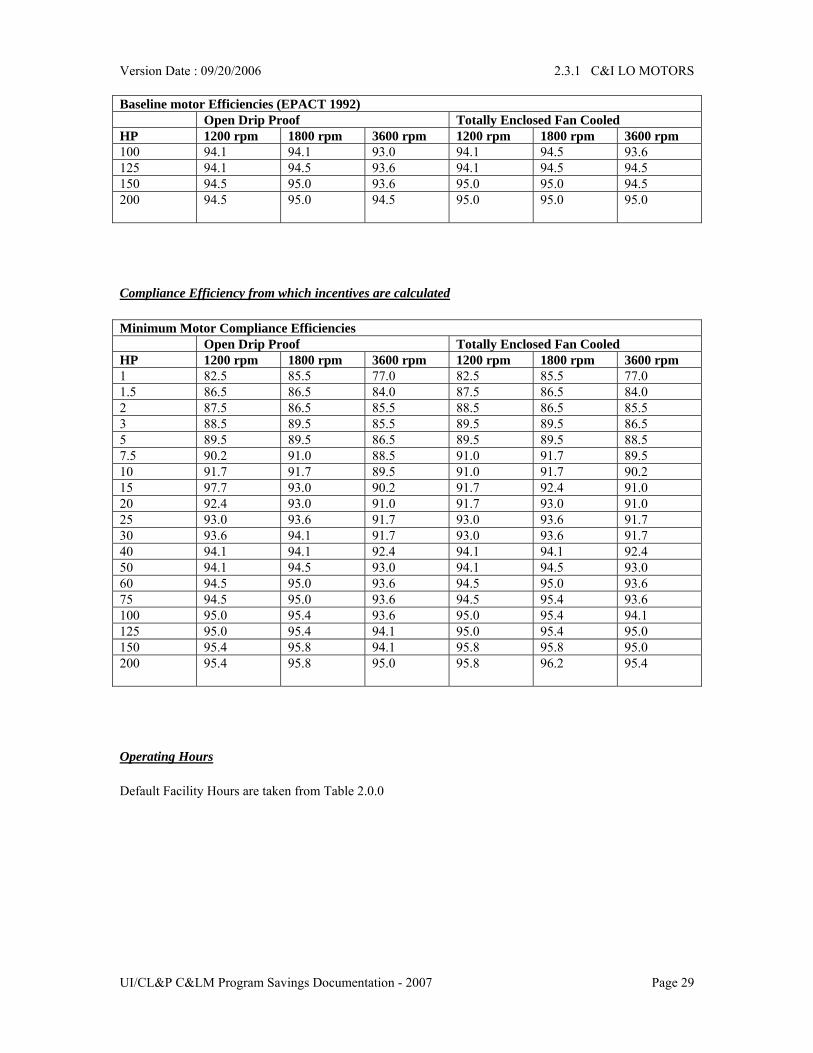
Method for Calculating Energy Savings Annual kWh savings = Hp (0.746 kW/hp) (D) (1/EFFb -1/EFFi) (HRS) Hp = motor’s rated horsepower D = Peak Factor from Table 1.1.1 EFFb = Baseline efficiency (see table below) EFFi = Installed motor efficiency (see table below) HRS = Annual Hours of operation
Method for Calculating Demand Savings kW savings = Hp (0.746 kW/hp) (D) (1/EFFb -1/EFFi)
Non-Electric Benefits - Annual Fossil Fuel Savings Non-electric benefits have not been identified for this measure.
Revision Number 03
Version Date : 09/20/2006 2.4.1 HVAC VFD
UI/CL&P C&LM Program Savings Documentation - 2007 Page 31
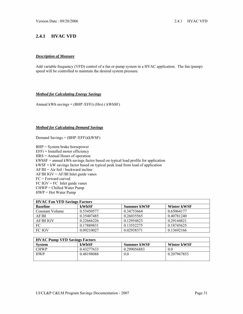
2.4.1 HVAC VFD
Description of Measure Add variable frequency (VFD) control of a fan or pump system in a HVAC application. The fan (pump) speed will be controlled to maintain the desired system pressure.
Method for Calculating Energy Savings Annual kWh savings = (BHP /EFFi) (Hrs) ( kWhSF)
Method for Calculating Demand Savings Demand Savings = (BHP /EFFi)(kWSF) BHP = System brake horsepower EFFi = Installed motor efficiency HRS = Annual Hours of operation kWhSF = annual kWh savings factor based on typical load profile for application kWSF = kW savings factor based on typical peak load from load of application AF/BI = Air foil / backward incline AF/BI IGV = AF/BI Inlet guide vanes FC = Forward curved FC IGV = FC Inlet guide vanes CHWP = Chilled Water Pump HWP = Hot Water Pump HVAC Fan VFD Savings Factors Baseline kWhSF Summer kWSF Winter kWSF Constant Volume 0.53450577 0.34753664 0.65064177 AF/BI 0.35407485 0.26035565 0.40781240 AF/BI IGV 0.22666226 0.12954823 0.29144821 FC 0.17889831 0.13552275 0.18745625 FC IGV 0.09210027 0.02938371 0.13692166 HVAC Pump VFD Savings Factors System kWhSF Summer kWSF Winter kWSF CHWP 0.43277633 0.299056883 0.0 HWP 0.48198088 0.0 0.207967853
Version Date : 09/20/2006 2.4.1 HVAC VFD
UI/CL&P C&LM Program Savings Documentation - 2007 Page 32
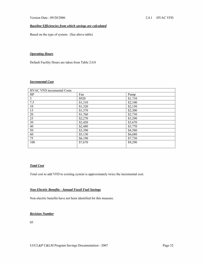
Baseline Efficiencies from which savings are calculated Based on the type of system. (See above table)
Operating Hours Default Facility Hours are taken from Table 2.0.0
Total Cost Total cost to add VFD to existing system is approximately twice the incremental cost.
Non-Electric Benefits - Annual Fossil Fuel Savings Non-electric benefits have not been identified for this measure.
Revision Number 05
Version Date : 09/20/2006 2.5.1 ICE-CUBE MAKERS
UI/CL&P C&LM Program Savings Documentation - 2007 Page 33
2.5.1 ICE-CUBE MAKERS
Description of Measure This measure encourages the installation of efficient commercial ice-cube machines. It is based on the Consortium for Energy Efficiency’s (CEE) guidelines, which is based, in turn, on FEMP guidelines.
Method for Calculating Energy Savings For each ice-making machine proposed for this measure, the ice harvest rate, the energy consumption rate and the type of machine are needed.
365100
•−
= RAES
S = Savings, kWh per year E = Baseline energy use rate, kWh per 100 lb of ice produced. A = Actual energy use rate, kWh per 100 lb of ice produced. 100 = Conversion to kWh per lb. R = Ice harvest rate, lb per day. 365 = Conversion to kWh per year.
Method for Calculating Demand Savings
24100RAEkW •
−=
kW = Demand savings, kw E = Baseline energy use rate, kWh per 100 lb of ice produced. A = Actual energy use rate, kWh per 100 lb of ice produced. 100 = Conversion to kWh per lb. R = Ice harvest rate, lb per day. 24 = Conversion to kw.
Baseline Efficiencies from which savings are calculated The baseline efficiency is taken from the CEE program. These values are derived from FEMP. 1/11/2005 Baseline Energy Rate , E, kwh/100lb
Type Type Description Up To R, lb/day E= Otherwise, E=
Version Date : 09/20/2006 2.5.1 ICE-CUBE MAKERS
UI/CL&P C&LM Program Savings Documentation - 2007 Page 34
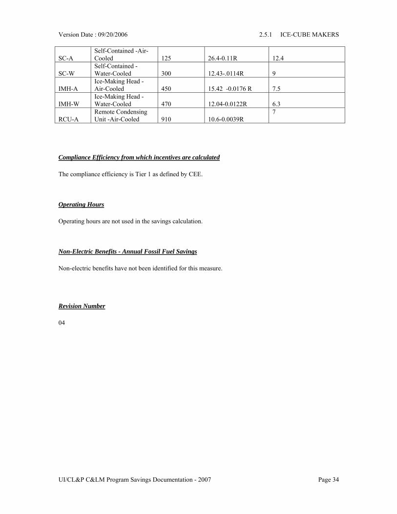
IMH-A Ice-Making Head -Air-Cooled 450 15.42 -0.0176 R 7.5
IMH-W Ice-Making Head -Water-Cooled 470 12.04-0.0122R 6.3
RCU-A Remote Condensing Unit -Air-Cooled 910 10.6-0.0039R
7
Compliance Efficiency from which incentives are calculated The compliance efficiency is Tier 1 as defined by CEE.
Operating Hours Operating hours are not used in the savings calculation.
Non-Electric Benefits - Annual Fossil Fuel Savings Non-electric benefits have not been identified for this measure.
Revision Number 04
Version Date : 09/20/2006 2.5.2 SOLID-DOOR REFRIGERATORS AND
UI/CL&P C&LM Program Savings Documentation - 2007 Page 35
2.5.2 SOLID-DOOR REFRIGERATORS AND FREEZERS
Description of Measure This measure encourages the installation of efficient commercial refrigerators and freezers with solid-doors. It is based on the Consortium for Energy Efficiency’s (CEE) guidelines, which is based, in turn, on FEMP guidelines.
Method for Calculating Energy Savings For each commercial refrigerator or freezer with solid-doors proposed for this measure, the internal volume, the energy consumption rate and the type of machine are needed. S = E – A(365) S = Savings, kWh per year E = Baseline energy use rate, kWh per year. A = Actual energy use rate, kWh per day. The value of A is provided by CEE for each make, size, and type of equipment.
Method for Calculating Demand Savings
8760SkW =
S = Savings, kWh per year 8760 = No. of hours per year
Baseline Efficiencies from which savings are calculated The Baseline Energy Use Rate, kWh/yr, for Solid-Door refrigerators is: E = Internal Volume times 45.624 + 1007 The Baseline Energy Use Rate, kWh/yr, for Solid-Door freezers is: E = Internal Volume times 145.25 + 833 These equations are derived from CEE data, and will be updated as appropriate.
Version Date : 09/20/2006 2.5.2 SOLID-DOOR REFRIGERATORS AND
UI/CL&P C&LM Program Savings Documentation - 2007 Page 36
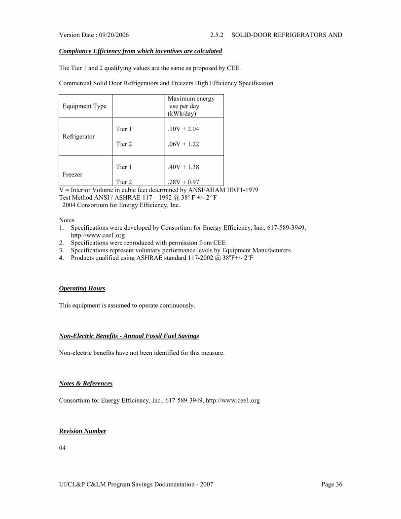
Compliance Efficiency from which incentives are calculated The Tier 1 and 2 qualifying values are the same as proposed by CEE. Commercial Solid Door Refrigerators and Freezers High Efficiency Specification
Equipment Type
Maximum energy use per day (kWh/day)
Refrigerator
Tier 1 Tier 2
.10V + 2.04 .06V + 1.22
Freezer
Tier 1 Tier 2
.40V + 1.38 .28V + 0.97
V = Interior Volume in cubic feet determined by ANSI/AHAM HRF1-1979 Test Method ANSI / ASHRAE 117 – 1992 @ 38o F +/- 2o F 2004 Consortium for Energy Efficiency, Inc. Notes 1. Specifications were developed by Consortium for Energy Efficiency, Inc., 617-589-3949,
http://www.cee1.org 2. Specifications were reproduced with permission from CEE 3. Specifications represent voluntary performance levels by Equipment Manufacturers 4. Products qualified using ASHRAE standard 117-2002 @ 38oF+/- 2oF
Operating Hours This equipment is assumed to operate continuously.
Non-Electric Benefits - Annual Fossil Fuel Savings Non-electric benefits have not been identified for this measure.
Notes & References Consortium for Energy Efficiency, Inc., 617-589-3949, http://www.cee1.org
Revision Number 04
Version Date : 09/20/2006 2.5.3 GLASS-DOOR REFRIGERATORS
UI/CL&P C&LM Program Savings Documentation - 2007 Page 37
2.5.3 GLASS-DOOR REFRIGERATORS
Description of Measure This measure encourages the installation of efficient commercial refrigerators with glass doors. It is based on the Consortium for Energy Efficiency’s (CEE) guidelines, which is based, in turn, on FEMP guidelines.
Method for Calculating Energy Savings For each refrigerator proposed for this measure, the annual energy savings is supplied directly by CEE based on the internal volume. For Refrigerators meeting Tier 1 standards, S = 19V+521 For Refrigerators meeting Tier 2 standards, S = 50.6V+112.3 S = Savings, kWh per year V = Internal volume, cu. ft.
Method for Calculating Demand Savings
8760SkW =
S = Savings, kWh per year 8760 = No. of hours per year
Baseline Efficiencies from which savings are calculated The baseline efficiency is assumed by CEE to be the least-efficient equipment on the market, and is included in the equation for energy savings.
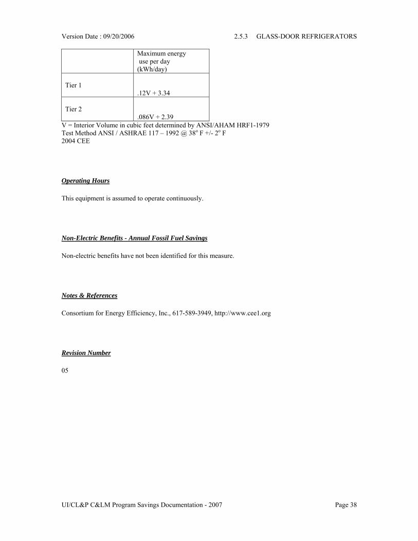
Compliance Efficiency from which incentives are calculated Commercial Glass Door, Reach-In High Efficiency Specification
Version Date : 09/20/2006 2.5.3 GLASS-DOOR REFRIGERATORS
UI/CL&P C&LM Program Savings Documentation - 2007 Page 38
Maximum energy use per day (kWh/day)
Tier 1
.12V + 3.34
Tier 2
.086V + 2.39
V = Interior Volume in cubic feet determined by ANSI/AHAM HRF1-1979 Test Method ANSI / ASHRAE 117 – 1992 @ 38o F +/- 2o F 2004 CEE
Operating Hours This equipment is assumed to operate continuously.
Non-Electric Benefits - Annual Fossil Fuel Savings Non-electric benefits have not been identified for this measure.
Notes & References Consortium for Energy Efficiency, Inc., 617-589-3949, http://www.cee1.org
Revision Number 05
Version Date : 09/20/2006 2.5.4 VENDING MACHINE OCCUPANCY CONTROLS
UI/CL&P C&LM Program Savings Documentation - 2007 Page 39
2.5.4 VENDING MACHINE OCCUPANCY CONTROLS
Description of Measure Installation of vending machine occupancy sensor.
Method for Calculating Energy Savings Annual savings = 1,600 kWh Savings are based on a 2001 study done by the Nicholas Group, P.C..
Method for Calculating Demand Savings Demand savings = 0
Baseline Efficiencies from which savings are calculated Existing vending machine operating without the occupancy sensor control.
Incremental Cost $75 per unit
Non-Electric Benefits - Annual Fossil Fuel Savings Non-electric benefits have not been identified for this measure.
Revision Number 02
Version Date : 09/20/2006 2.6.1 COMPUTER POWER SUPPLY
UI/CL&P C&LM Program Savings Documentation - 2007 Page 40
2.6.1 COMPUTER POWER SUPPLY
Description of Measure Computers with a more efficient power supply.
Method for Calculating Energy Savings Savings are based on estimates of a typical computer’s usage. Study provided by the Ecos Group. Annual kWh savings = 85 kWh/computer
Non-Electric Benefits - Annual Fossil Fuel Savings Non-electric benefits have not been identified for this measure.
Revision Number 02
Version Date : 09/20/2006 2.7.1 LEAN MANUFACTURING
UI/CL&P C&LM Program Savings Documentation - 2007 Page 41
2.7.1 LEAN MANUFACTURING
Description of Measure Incorporating PRIME (LEAN) in the manufacturing process allows a company to produce more in the same given time period. The savings are based on estimating the production increase with and without PRIME. Savings are based on two concepts: 1) Producing the more products in the same time period saves on the non- manufacturing consumption (mostly lighting). 2) Producing more products over the same time period reduces losses in the manufacturing equipment consumption (Less idle time, motors loaded more are more efficient. Note: The PRIME process also reduces waste. Since this is very site dependent it typically is not considered in this calculation.
Method for Calculating Energy Savings Annual Kwh savings = (EACWoP – EACWP) Baseline: EACWoP: Estimated annual consumption without PRIME at increased production levels EACWoP = Production kWh + Office kWh + Other kWh Production kWh = 0.75 (PPA) (AkWh) ( PAP/EP) Office kWh = 0.05 (PPA) (AkWh) Other kWh = 0.20 (PPA) (AkWh) (PAP/EP) EACWP = Estimated annual consumption with PRIME at increased production levels EACWP = Production kWh + Office kWh + Other kWh Production kWh = 0.75 (PPA) (AkWh) (1+(1/EP)(0.94)(PAP-EP)) Office kWh = 0.05 (PPA) (AkWh) Other kWh = 0.20 (PPA) (AkWh) PPA = Percentage of facility’s total products affected By PRIME AkWh = Existing annual kWh PAP = number of products produced after PRIME EP = existing number of products produced
Method for Calculating Demand Savings kW Savings = 0
Baseline Efficiencies from which savings are calculated
Version Date : 09/20/2006 2.7.1 LEAN MANUFACTURING
UI/CL&P C&LM Program Savings Documentation - 2007 Page 42
Baseline is calculated existing production methodology with increased production levels.
Operating Hours Not used in calculation.
Incremental Cost None
Non-Electric Benefits - Annual Fossil Fuel Savings Non-electric benefits have not been identified for this measure.
Non-Electric Benefits - Annual O&M Cost Adjustments The customer’s cost savings from the increase in productivity and reduction in scrap would be quantified on a case by case basis.
Notes & References Savings calculation is preliminary for 2007. May be modified based on ERS study. Measure life will be 5 years.
Revision Number 04
Version Date : 09/20/2006 2.7.3 RENEWABLE - GRID CONNECTED
UI/CL&P C&LM Program Savings Documentation - 2007 Page 43
2.7.3 RENEWABLE - GRID CONNECTED
Description of Measure This measure provides an incentive for renewable energy that is connected to the electric power grid. The incentive is available for solar photovoltaic, wind turbines, biomass-conversion power production and other such technologies.
Method for Calculating Energy Savings S = (Net kW) (Capacity Factor) (8760) S = Energy produced by the renewable source that ordinarily would have been supplied by the grid. Net KW = The renewable power that is available to supply external loads. For solar, for instance, the Net KW is the power available at the output terminals of the inverter. Capacity Factor = The portion of the year that the renewable source would require to produce its total annual energy if it was able to operate at full output for the entire time. A typical CF for solar would be less than 20%, and wind less than 25%. 8760 = The number of hours in a year.
Method for Calculating Demand Savings KW = 0.5 (Net kW) KW = Amount by which the grid load is reduced at the time of the summer peak Net KW = The renewable power that is available to supply external loads.
Operating Hours For solar and wind, the capacity factor is estimated from meteorological data and the experience of similar projects. The CF would be part of the economic analysis of the project’s viability. For other types of renewable power, such as biomass conversion, the capacity factor will depend on the technology, the planned operating scenarios, the fuel availability and other factors. It will have to be determined on a case-by-case basis.
Total Cost The total installed cost of the renewable power.
Version Date : 09/20/2006 2.7.3 RENEWABLE - GRID CONNECTED
UI/CL&P C&LM Program Savings Documentation - 2007 Page 44
Non-Electric Benefits - Annual Fossil Fuel Savings Non-electric benefits have not been identified for this measure.
Revision Number 01
Version Date : 09/20/2006 2.7.3 RENEWABLE - GRID CONNECTED
UI/CL&P C&LM Program Savings Documentation - 2007 Page 45
C&I RETROFIT
Version Date : 09/20/2006 3.1.1 STANDARD LIGHTING
UI/CL&P C&LM Program Savings Documentation - 2007 Page 46
3.1.1 STANDARD LIGHTING
Description of Measure This measure provides an incentive to replace inefficient lighting with efficient lighting.
Method for Calculating Energy Savings S = (kWB –kWA) H S = Energy savings, kwh/year kWB = The total power usage of the lighting fixtures that are being replaced, kW. kWA = The total power usage of the new lighting fixtures that are being installed, kW. H = The number of hours during which the lighting is used at the facility, hours/year.
Method for Calculating Demand Savings KW = D* (kWB –kWA) D = Peak factor from Table 1.1.1
Baseline Efficiencies from which savings are calculated There are no set baseline and compliance efficiencies. The energy savings are calculated as the difference between what is observed before this measure is installed and what is observed after this measure is installed.
Compliance Efficiency from which incentives are calculated There are no set baseline and compliance efficiencies. The energy savings are calculated as the difference between what is observed before this measure is installed and what is observed after this measure is installed.
Operating Hours The operating hours are determined on a case-by-case basis, or the default facility hours are used from Table 2.0.0.
Version Date : 09/20/2006 3.1.1 STANDARD LIGHTING
UI/CL&P C&LM Program Savings Documentation - 2007 Page 47
Total Cost The cost to install the measure.
Non-Electric Benefits - Annual Fossil Fuel Savings Space heating increase from reduced lighting load. Annual Fossil fuel Savings = -0.00079 MBTU’s per annual kWh saved. Based on August 22, 2003 Memorandum from Optimal energy, Inc..
Non-Electric Benefits - Annual O&M Cost Adjustments O&M savings are due to the installation of new equipment. O&M Savings = $0.003667 per annual kWh saved. Based on August 22, 2003 Memorandum from Optimal energy, Inc..
Revision Number 04
Version Date : 09/20/2006 3.2.1 COOLING - CHILLERS
UI/CL&P C&LM Program Savings Documentation - 2007 Page 48
3.2.1 COOLING - CHILLERS
Description of Measure This measure encourages the installation of efficient water-cooled and air-cooled water chilling packages (chillers) as replacements for less-efficient chillers. Chillers must use an environmentally friendly refrigerant in order to qualify for the program.
Method for Calculating Energy Savings The energy consumption is custom-calculated for each chiller installation based on the specific equipment, operational staging, operating profile, and load profile. These calculations are performed for both the old chiller plant and the new chiller plant. The difference in energy consumption between the two plants is the energy savings. Equipment Each chiller plant is characterized by its:
• Number of chillers, • Sizes, in tons (the chillers may be of different sizes), • Type, which may be:
o Centrifugal, R123 refrigerant, R134a refrigerant
o Water-cooled screw and scroll, or o Air-cooled
• Speed, constant or variable • Auxiliary equipment
o Chilled water pumps o Cooling tower pumps o Cooling tower fans o Other
Operational Staging If more than one chiller is used, their operational relationship can be defined. When the load is high enough to permit two chillers to operate, they can be designated to operate together at the same loading, or, alternatively, either one can be operated at full output and the other can follow the cooling load profile. Operating Profile The customer’s cooling load profile, for each of 12 months, is characterized by the:
• On-peak occupied hours the chiller is operated each week, • Off-peak occupied hours the chiller is operated each week, • On-peak un-occupied hours the chiller is operated each week, • Off-peak un-occupied hours the chiller is operated each week.
Version Date : 09/20/2006 3.2.1 COOLING - CHILLERS
UI/CL&P C&LM Program Savings Documentation - 2007 Page 49
Load Profile The customer’s load profile is estimated by determining the load at the peak outdoor conditions and the load at the minimum conditions. For systems with an air-side or water-side economizer, the minimum conditions are those just above the set point of the economizer. If the customer’s load profile is not known, a default load profile will be developed; in this case it is also necessary to determine the value of any process loads. Savings Calculation With the above information, a calculation is made for each time period of the year based on the appropriate temperature bin data. The calculation is performed once for the old chillers and again for the proposed chillers, and the difference determines the kWh and the kW savings for each period. These are summed to yield the annual total savings for each year of the remaining life of the old chiller.
Method for Calculating Demand Savings The demand savings calculation is described in the previous paragraph.
Baseline Efficiencies from which savings are calculated Savings are calculated using the old chiller as the baseline.
Compliance Efficiency from which incentives are calculated The proposed replacement chiller rating at ARI conditions must meet a minimum efficiency to qualify for an incentive. The minimum is set at an efficiency somewhat better than what Ashrae 90.1 requires. These minimum efficiency levels for the various sizes and types of chillers are shown in Table 2.2.1.A in the Appendix. The ARI conditions are shown in Table 2.2.1.B in the Appendix.
Operating Hours A single value for operating hours is not used. As described above, custom hourly calculations are made for each customer.
Non-Electric Benefits - Annual Fossil Fuel Savings Non-electric benefits have not been identified for this measure.
Revision Number 05
Version Date : 09/20/2006 3.2.2 COOLING - HVAC
UI/CL&P C&LM Program Savings Documentation - 2007 Page 50
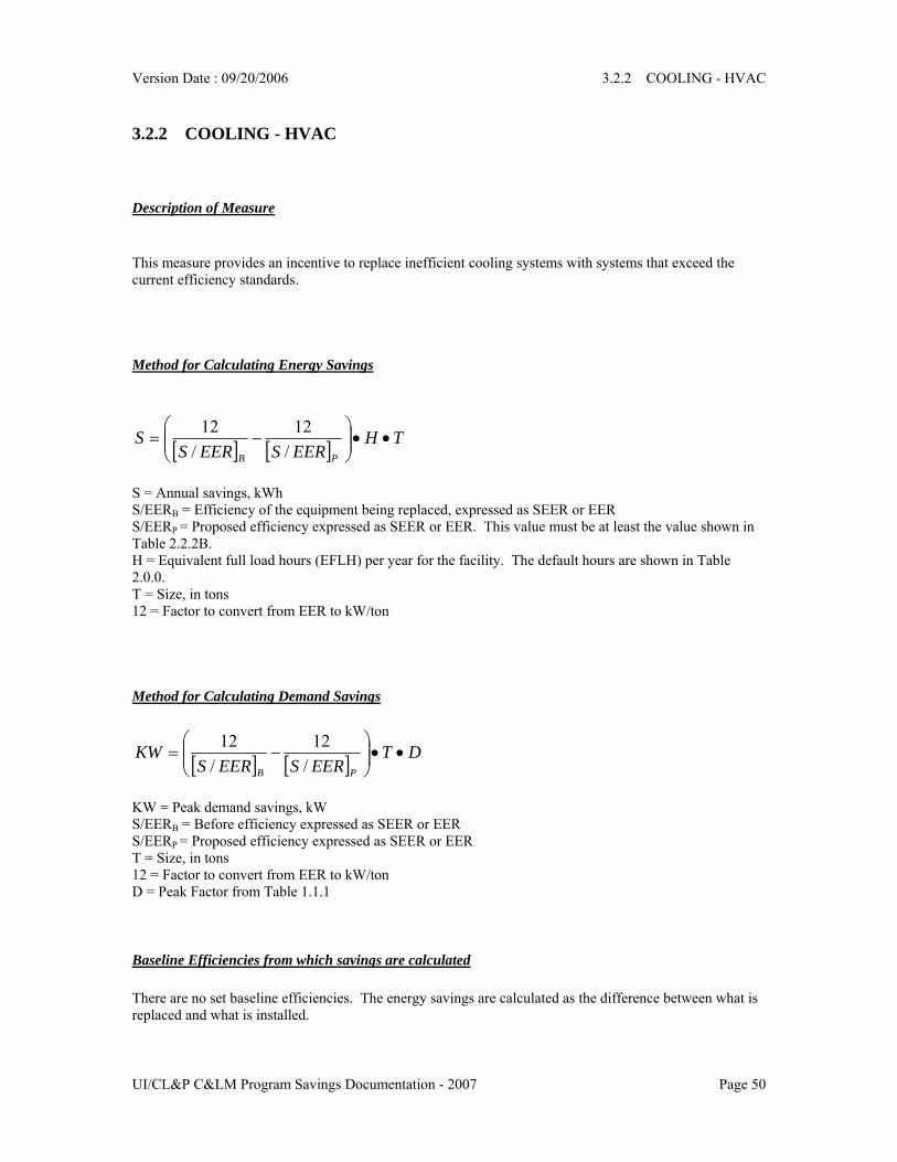
3.2.2 COOLING - HVAC
Description of Measure This measure provides an incentive to replace inefficient cooling systems with systems that exceed the current efficiency standards.
Method for Calculating Energy Savings
[ ] [ ] THEERSEERS
SPB
••⎟⎟⎠
⎞⎜⎜⎝
⎛−=
/12
/12
S = Annual savings, kWh S/EERB = Efficiency of the equipment being replaced, expressed as SEER or EER S/EERP = Proposed efficiency expressed as SEER or EER. This value must be at least the value shown in Table 2.2.2B. H = Equivalent full load hours (EFLH) per year for the facility. The default hours are shown in Table 2.0.0. T = Size, in tons 12 = Factor to convert from EER to kW/ton
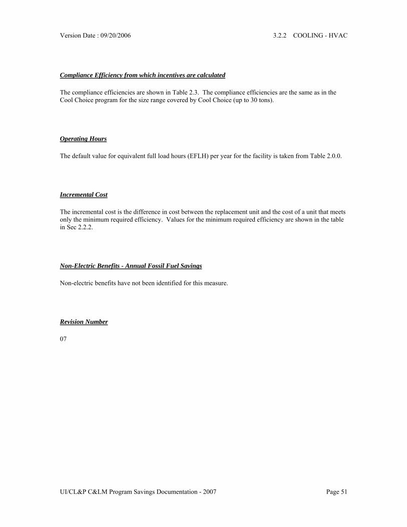
Method for Calculating Demand Savings
[ ] [ ] DTEERSEERS
KWPB
••⎟⎟⎠
⎞⎜⎜⎝
⎛−=
/12
/12
KW = Peak demand savings, kW S/EERB = Before efficiency expressed as SEER or EER S/EERP = Proposed efficiency expressed as SEER or EER T = Size, in tons 12 = Factor to convert from EER to kW/ton D = Peak Factor from Table 1.1.1
Baseline Efficiencies from which savings are calculated There are no set baseline efficiencies. The energy savings are calculated as the difference between what is replaced and what is installed.
Version Date : 09/20/2006 3.2.2 COOLING - HVAC
UI/CL&P C&LM Program Savings Documentation - 2007 Page 51
Compliance Efficiency from which incentives are calculated The compliance efficiencies are shown in Table 2.3. The compliance efficiencies are the same as in the Cool Choice program for the size range covered by Cool Choice (up to 30 tons).
Operating Hours The default value for equivalent full load hours (EFLH) per year for the facility is taken from Table 2.0.0.
Incremental Cost The incremental cost is the difference in cost between the replacement unit and the cost of a unit that meets only the minimum required efficiency. Values for the minimum required efficiency are shown in the table in Sec 2.2.2.
Non-Electric Benefits - Annual Fossil Fuel Savings Non-electric benefits have not been identified for this measure.
Revision Number 07
Version Date : 09/20/2006 3.3.1 CUSTOM MEASURE
UI/CL&P C&LM Program Savings Documentation - 2007 Page 52
3.3.1 CUSTOM MEASURE
Description of Measure This measure is used for C&I Retrofit installations not covered by another specific measure.
Method for Calculating Energy Savings Energy savings are calculated on a custom basis for each customer’s specific situation. The savings are the difference in energy usage between the before and after conditions.
Method for Calculating Demand Savings Measures may be lumped into two significantly different categories: 1.) Temperature-dependent (HVAC measures that vary with ambient temperature), 2.) Measures that are not temperature-dependent (process, lighting, time control). Temperature-dependent methodologies: The methodology used to determine the demand savings for temperature-dependent measures will depend on the type of analysis used to estimate the savings. Savings from temperature-dependent measures are typically determined by either full load hour analysis, bin temperature analysis, or a detailed computer simulation. The following will be the procedure used to estimate the demand savings for these measures: An appropriately derived coincidence factor, such as those in the RLW study referenced below, will be used for a measure that has a connected load that can be determined from rated or nameplate data. Demand savings will be the connected load kW times the appropriate coincidence factor. The demand (kW) savings estimated for the highest temperature bin will be used for the demand savings when a bin temperature analysis is used to calculate the energy savings and the appropriate coincidence factor is not available. The demand savings estimated by the computer simulation between 3 and 5 PM for the hottest day (defined as the day with the highest average enthalpy over the 3 to 5 PM window) will be used as the demand savings when a computer simulation is being used to estimate energy savings. Non-Temperature-dependent measures: Demand savings for measures that are not temperature-dependent will be determined by either the coincidence factors from Table 1.1.1 or the average estimated savings over the summer hours from 3 to 5 PM. For example, for a process VFD measure, the savings will depend on cycling of the load. This cycling may occur many times during an hour. If the process is operating between 3 and 5 PM during the summer, the average demand savings will be: (annual kWh savings)/(annual equivalent full load hours of operation).
Version Date : 09/20/2006 3.3.1 CUSTOM MEASURE
UI/CL&P C&LM Program Savings Documentation - 2007 Page 53
If the process is operated only a portion of that time period the demand savings will be prorated based on that portion.
Baseline Efficiencies from which savings are calculated There are no set baseline and compliance efficiencies. The energy savings are calculated as the difference between what is observed before this measure is installed and what is observed after this measure is installed.
Compliance Efficiency from which incentives are calculated There are no set baseline and compliance efficiencies. The energy savings are calculated as the difference between what is observed before this measure is installed and what is observed after this measure is installed.
Operating Hours The operating hours are determined on a case-by-case basis.
Total Cost The cost to install the measure.
Non-Electric Benefits - Annual Fossil Fuel Savings Non-electric benefits are analyzed on a case-by-case basis.
UI/CL&P C&LM Program Savings Documentation - 2007 Page 54
SMALL BUSINESS
Version Date : 09/20/2006 4.1.1 SMB STANDARD LIGHTING
UI/CL&P C&LM Program Savings Documentation - 2007 Page 55
4.1.1 SMB STANDARD LIGHTING
Description of Measure This measure provides an incentive to small businesses to replace inefficient lighting with efficient lighting.
Method for Calculating Energy Savings S = (kWB –kWA) H S = Energy savings, kwh/year kWB = The total power usage of the lighting fixtures that are being replaced, kW. kWA = The total power usage of the new lighting fixtures that are being installed, kW. H = The number of hours during which the lighting is used at the facility, hours/year.
Method for Calculating Demand Savings KW = D (kWB –kWA) D = Peak factor from Table 1.1.1
Baseline Efficiencies from which savings are calculated There are no set baseline and compliance efficiencies. The energy savings are calculated as the difference between what is observed before this measure is installed and what is observed after this measure is installed.
Compliance Efficiency from which incentives are calculated There are no set baseline and compliance efficiencies. The energy savings are calculated as the difference between what is observed before this measure is installed and what is observed after this measure is installed.
Operating Hours
Version Date : 09/20/2006 4.1.1 SMB STANDARD LIGHTING
UI/CL&P C&LM Program Savings Documentation - 2007 Page 56
The operating hours are determined on a case-by-case basis, or the default facility hours from Table 2.0.0 are used.
Total Cost The cost to install the measure.
Non-Electric Benefits - Annual Fossil Fuel Savings Space heating increase from reduced lighting load. Annual Fossil fuel Savings = -0.00079 MBTU’s per annual kWh saved. Based on August 22, 2003 Memorandum from Optimal energy, Inc..
Non-Electric Benefits - Annual O&M Cost Adjustments O&M savings are due to the installation of new equipment. O&M Savings = $0.003667 per annual kWh saved. Based on August 22, 2003 Memorandum from Optimal energy, Inc..
Revision Number 04
Version Date : 09/20/2006 4.2.1 SMB CUSTOM
UI/CL&P C&LM Program Savings Documentation - 2007 Page 57
4.2.1 SMB CUSTOM
Description of Measure This measure is used for Small Business installations not covered by another specific measure.
Method for Calculating Energy Savings Energy savings are calculated on a custom basis for each customer’s specific situation. The savings are the difference in energy usage between the before and after conditions.
Method for Calculating Demand Savings Demand savings are calculated on a custom basis for each customer’s specific situation. The savings is the difference in power demand between the before and after conditions that would occur due to the installation of the measure at the time of the electric system peak.
Baseline Efficiencies from which savings are calculated There are no set baseline and compliance efficiencies. The energy savings are calculated as the difference between what is observed before this measure is installed and what is observed after this measure is installed.
Compliance Efficiency from which incentives are calculated There are no set baseline and compliance efficiencies. The energy savings are calculated as the difference between what is observed before this measure is installed and what is observed after this measure is installed.
Operating Hours The operating hours are determined on a case-by-case basis.
Version Date : 09/20/2006 4.2.1 SMB CUSTOM
UI/CL&P C&LM Program Savings Documentation - 2007 Page 58
Total Cost The cost to install the measure.
Non-Electric Benefits - Annual Fossil Fuel Savings Non-electric benefits have not been identified for this measure.
Revision Number 02
Version Date : 09/20/2006 4.2.2 SMB AC TUNEUP
UI/CL&P C&LM Program Savings Documentation - 2007 Page 59
4.2.2 SMB AC TUNEUP
Description of Measure This measure encourages users of Air Conditioning equipment to procure maintenance for their equipment from a service organization that uses a computer-based diagnostic tool. The computer-based diagnostic tool is the property of a third-party vendor, and analysis of the data is part of the service the vendor provides. Use of the computer diagnostics helps to ensure that the service is appropriate and complete.
Method for Calculating Energy Savings The kW savings for each customer is multiplied by the that facility’s specific EFLH value. KWh = kW*EFLH KWh = kWh energy savings per year KW = kW savings EFLH = Equivalent full-load hours of operation per year, based on facility type or customer-specific information.
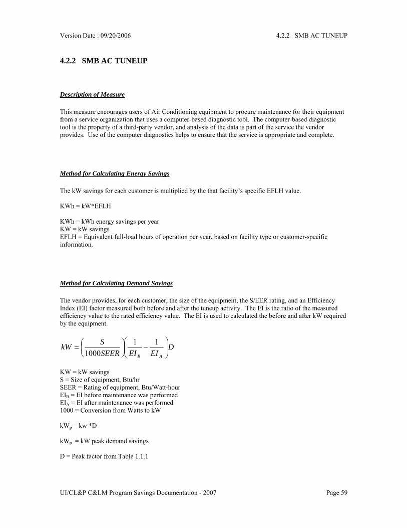
Method for Calculating Demand Savings The vendor provides, for each customer, the size of the equipment, the S/EER rating, and an Efficiency Index (EI) factor measured both before and after the tuneup activity. The EI is the ratio of the measured efficiency value to the rated efficiency value. The EI is used to calculated the before and after kW required by the equipment.
DEIEISEER
SkWAB⎟⎟⎠
⎞⎜⎜⎝
⎛−⎟
⎠⎞
⎜⎝⎛=
111000
KW = kW savings S = Size of equipment, Btu/hr SEER = Rating of equipment, Btu/Watt-hour EIB = EI before maintenance was performed EIA = EI after maintenance was performed 1000 = Conversion from Watts to kW kWp = kw *D kWp = kW peak demand savings D = Peak factor from Table 1.1.1
Version Date : 09/20/2006 4.2.2 SMB AC TUNEUP
UI/CL&P C&LM Program Savings Documentation - 2007 Page 60
Baseline Efficiencies from which savings are calculated No baseline is used for the energy savings; the savings are specific to each customer.
Compliance Efficiency from which incentives are calculated Incentives are not calculated based on the improvement of efficiency; they are based on a uniform payment for each piece of equipment that has been serviced.
Operating Hours Each facility type is assigned a default value for EFLH, as shown in Table 2.0.0.
Non-Electric Benefits - Annual Fossil Fuel Savings Non-electric benefits have not been identified for this measure.
Revision Number 07
Version Date : 09/20/2006 4.3.1 SMB EVAPORATOR FANS
UI/CL&P C&LM Program Savings Documentation - 2007 Page 61
4.3.1 SMB EVAPORATOR FANS
Description of Measure This measure is applicable to walk-in coolers and freezers that have evaporator fans that run constantly. The measure adds a control system to an existing facility. The control system shuts off the evaporator fans when the cooler’s thermostat is not calling for cooling.
Method for Calculating Energy Savings A custom calculation is performed for each facility. S = N*P*H*factors S = energy savings, kwh N = Number of fans P = Fan power, kw H = Hours per year the fans are shut off Factors = Other variables to take into account the motor efficiency, the number of phases, and the compressor efficiency
Method for Calculating Demand Savings KW = C*P KW = kw reduction from the summer peak C is the diversity factor of 10% P = Fan power, kw
Baseline Efficiencies from which savings are calculated The baseline is 24-hour operation of the fans.
Operating Hours Hours per year the fans are shut off.
Version Date : 09/20/2006 4.3.1 SMB EVAPORATOR FANS
UI/CL&P C&LM Program Savings Documentation - 2007 Page 62
Total Cost This is based on standard prices for the equipment that is installed.
Non-Electric Benefits - Annual Fossil Fuel Savings Non-electric benefits have not been identified for this measure.
Revision Number 03
Version Date : 09/20/2006 4.3.2 SMB DOOR HEATERS
UI/CL&P C&LM Program Savings Documentation - 2007 Page 63
4.3.2 SMB DOOR HEATERS
Description of Measure This measure is applicable to walk-in coolers and freezers that have electric heaters on the doors whose purpose is to prevent condensation from forming. This measure adds a control system to an existing facility whose door heaters operate continuously. The control system shuts off the door heaters when the facility’s humidity is too low to allow condensation to occur.
Method for Calculating Energy Savings S = P*6500 S = energy savings, kwh P = Door heater power, kw 6500 = Hours per year the heaters are shut off
Method for Calculating Demand Savings KW = D*P KW = kW reduction from the summer peak D is the estimated diversity factor of 10% P = Door heater power, kW
Baseline Efficiencies from which savings are calculated The baseline is 24-hour operation of the heaters.
Operating Hours Hours per year the heaters are shut off.
Total Cost The total cost is based on standard prices for the equipment that is installed.
Version Date : 09/20/2006 4.3.2 SMB DOOR HEATERS
UI/CL&P C&LM Program Savings Documentation - 2007 Page 64
Non-Electric Benefits - Annual Fossil Fuel Savings Non-electric benefits have not been identified for this measure.
Revision Number 03
Version Date : 09/20/2006 4.3.3 SMB VENDING MACHINE CENTRAL
UI/CL&P C&LM Program Savings Documentation - 2007 Page 65
4.3.3 SMB VENDING MACHINE CENTRAL CONTROLS
Description of Measure This measure is available for vending machines that are controlled by a central controller.
Method for Calculating Energy Savings S = kW( HB – HA) S = Energy savings, kwh/year kW = The total power usage of the vending machines that are being controlled, kW. HB = The number of hours before being controlled during which the vending machines are turned on at the facility, hours/year. This value is usually 8760. HA = The number of hours after the controls are installed during which the vending machines are turned on at the facility, hours/year.
Method for Calculating Demand Savings There are no demand savings for this measure.
Baseline Efficiencies from which savings are calculated There are no set baseline and compliance efficiencies. The energy savings are calculated as the difference between what is observed before this measure is installed and what is observed after this measure is installed.
Compliance Efficiency from which incentives are calculated There are no set baseline and compliance efficiencies. The energy savings are calculated as the difference between what is observed before this measure is installed and what is observed after this measure is installed.
Operating Hours The operating hours are determined on a case-by-case basis.
Version Date : 09/20/2006 4.3.3 SMB VENDING MACHINE CENTRAL
UI/CL&P C&LM Program Savings Documentation - 2007 Page 66
Total Cost The cost to install the measure.
Non-Electric Benefits - Annual Fossil Fuel Savings Non-electric benefits have not been identified for this measure.
Revision Number 02
Version Date : 09/20/2006 4.3.3 SMB VENDING MACHINE CENTRAL
UI/CL&P C&LM Program Savings Documentation - 2007 Page 67
RESIDENTIAL
Version Date : 09/20/2006 5.1.1 CFL LIGHT BULB (E-STAR HOMES)
UI/CL&P C&LM Program Savings Documentation - 2007 Page 68
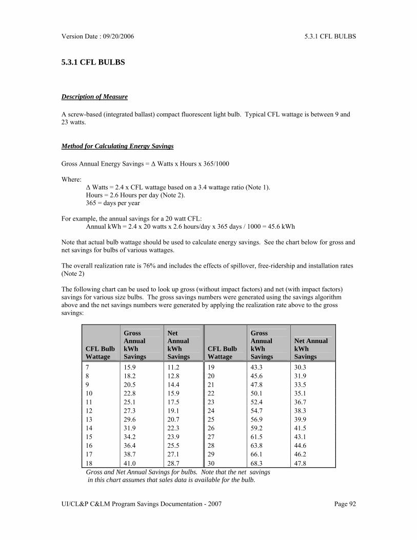
5.1.1 CFL LIGHT BULB (E-STAR HOMES)
Description of Measure A direct installed screw-based CFL bulb. “Direct installed” bulbs are either supplied to the builder for use in qualifying new homes or installed during the final inspection. Savings does not apply to bulbs that are placed in closets or non-living spaces (attics, unconditioned basements, etc.).
Method for Calculating Energy Savings Annual Energy Savings = Δ Watts x Hours x 365/1000 Where: Δ Watts = 2.4 x CFL wattage. This represents an “incandescent to CFL” wattage ratio of 3.4 to 1. Hours = 2.6 Hours per day (See Note 1) 365 = days per year For example, the annual savings for a 20 watt CFL: Annual kWh = 2.4 x 20 watts x 2.6 hours/day x 365 days / 1000 = 45.5 kWh Note that actual bulb wattage should be used to calculate energy savings – using a default average could lead to a large margin of error. The following chart can be used to calculate the savings for various size bulbs:
Version Date : 09/20/2006 5.1.1 CFL LIGHT BULB (E-STAR HOMES)
UI/CL&P C&LM Program Savings Documentation - 2007 Page 69
Method for Calculating Demand Savings The demand savings is calculated by multiplying the annual kWh savings by the peak kW/kWh factor for residential lighting found in Appendix Table 1.1.
Baseline Efficiencies from which savings are calculated Baseline is assumed to be an incandescent light source with a wattage which is 3.4 times higher than the wattage of the CFL bulb. For instance, it’s assumed that a 75 Watt incandescent is “equivalent” to a 22 Watt CFL (22 x 3.4 = 75). For dimmable or three-way CFL bulbs, assume the highest wattage/setting when calculating the baseline equivalent.
Compliance Efficiency from which incentives are calculated Energy Star CFL Bulb.
Operating Hours 2.6 Hours per day.
Incremental Cost $3.00
Non-Electric Benefits - Annual O&M Cost Adjustments $4.00 per bulb one time benefit. Estimate based on current cost of incandescent bulbs that would be used in place of one CFL.
Notes & References Note 1. Northeast Utilities and United Illuminating Retail/Point of Purchase Lighting Program Impact Evaluation, RLW Analytics, April 2003.
Revision Number 03
Version Date : 09/20/2006 5.1.2 CFL FIXTURES (E-STAR HOMES)
UI/CL&P C&LM Program Savings Documentation - 2007 Page 70
5.1.2 CFL FIXTURES (E-STAR HOMES)
Description of Measure An Energy Star hardwired fluorescent fixture with pin based bulbs. Fixtures with screw-based (CFL) bulbs are treated as CFL bulbs for savings calculations.
Method for Calculating Energy Savings Annual Energy Savings = Δ Watts x Hours x 365/1000 Where: Δ Watts = 2.4 x fixture wattage (a 3.4 wattage conversion factor). Hours = 3.2 Hours per day (Note 1) 365 = days per year For example, the annual savings for a 25 watt fixture: Annual kWh = 2.4 x 25 watts x 3.2 hours/day x 365 days / 1000 = 70.1 kWh
Method for Calculating Demand Savings The peak demand savings is calculated by multiplying the annual kWh by the peak demand factor for residential lighting found in Appendix Table 1.1.
Baseline Efficiencies from which savings are calculated Incandescent fixture with a wattage equal to 3.4 times the wattage of the efficient fluorescent fixture. For dimmable or three-way CFL bulbs, assume the highest wattage/setting when calculating the baseline equivalent.
Compliance Efficiency from which incentives are calculated Energy Star hard-wired fixture with equivalent lumen output.
Operating Hours 3.2 hours per day from RLW 2003 Lighting Evaluation (Note 1).
Version Date : 09/20/2006 5.1.2 CFL FIXTURES (E-STAR HOMES)
UI/CL&P C&LM Program Savings Documentation - 2007 Page 71
Incremental Cost $10
Non-Electric Benefits - Annual Fossil Fuel Savings Non-electric benefits have not been identified for this measure.
Non-Electric Benefits - Annual O&M Cost Adjustments $14.00 (one-time benefit per fixture). Estimate based on added cost of using incandescent bulbs over the life of the measure.
Notes & References Note 1. Northeast Utilities and United Illuminating Retail/Point of Purchase Lighting Program Impact Evaluation, RLW Analytics, April 2003.
Revision Number 02
Version Date : 09/20/2006 5.2.1 SEER 14 MIN AC
UI/CL&P C&LM Program Savings Documentation - 2007 Page 72
5.2.1 SEER 14 MIN AC
Description of Measure Central AC system with rated efficiency of 14 SEER or higher.
Method for Calculating Energy Savings
A. New Construction: Annual Energy Savings = 500 x size (1/13 – 1/SEER) / 1000 Where: 500 = expected annual full-run hours (Note 1). Size = size of system in Btu 13 = assumed SEER (efficiency) of baseline equipment. SEER = rated SEER (efficiency) of efficient equipment For example, for a 3 ton (36,000 Btu) 14 SEER system, the annual kWh savings would be = 500 x 36,000 x (1/13 – 1/14) / 1000 = 98.9 kWh. The following chart can be used as a reference to look up the savings for new units:
Size 14 SEER
15 SEER
16 SEER
17 SEER
1 ton 33.0 61.5 86.5 108.6 2 ton 65.9 123.1 173.1 217.2 3 ton 98.9 184.6 259.6 325.8 4 ton 131.9 246.2 346.2 434.4 5 ton 164.8 307.7 432.7 543.0
Expected annual kWh cooling savings for various sizes and efficiency of units Note 1: The above chart on energy savings also applies to the Ductless Mini Splits Heat Pump equipments. Note 2: For multi-speed units, a weighted average of the high speed and low speed efficiencies should be used. Assume 70% on low speed and 30% on high speed.
B. Early Retirement: If the contractor identifies an old central air unit still working and the customer agrees to replace it then a savings can be claimed for removing old unit and installing an Energy Star Unit. The measure life for these scenarios is estimated to be 7 years. The following chart can be used as a reference to look up the savings for Early Retirement of old units: Annual Energy Savings = 500 x size (1/Old SEER – 1/New SEER) / 1000 Where: 500 = expected annual full-run hours (Note 1).
Version Date : 09/20/2006 5.2.1 SEER 14 MIN AC
UI/CL&P C&LM Program Savings Documentation - 2007 Page 73
Size = size of system in Btu Old SEER = Rated SEER (efficiency) of the old unit being replaced. New SEER = Rated SEER (efficiency) of efficient equipment. The measure life in case of Retrofit is assumed to be 7 years Table: Annual Energy savings in kWh per ton
Method for Calculating Demand Savings The peak demand savings is calculated by multiplying the annual kWh savings by the peak kW/kWh factor for cooling found in Appendix Table 1.1.
Baseline Efficiencies from which savings are calculated A 13 SEER (code minimum) system.
Compliance Efficiency from which incentives are calculated 14 SEER or higher (Note 1).
Operating Hours 500 hours per year.
Version Date : 09/20/2006 5.2.1 SEER 14 MIN AC
UI/CL&P C&LM Program Savings Documentation - 2007 Page 74
Incremental Cost $100 per SEER unit per ton above 13. For example, a 3 ton 15 SEER would have an assumed incremental cost of $600.
Non-Electric Benefits - Annual Fossil Fuel Savings Non-electric benefits have not been identified for this measure.
Notes & References Note 1. Estimated based on Market Research for the Rhode Island, Massachusetts, and Connecticut Residential HVAC Market, RLW Analytics, December 2002, and supported by ASHRAE hours of use when corrected for oversizing.
Revision Number 04
Version Date : 09/20/2006 5.2.2 E-STAR HEAT PUMP
UI/CL&P C&LM Program Savings Documentation - 2007 Page 75
5.2.2 E-STAR HEAT PUMP
Description of Measure A heat pump with a heating season performance factor (HSPF) of 8.5 or higher. Note only the heating savings is presented here; cooling savings from an efficient heat pump is the same as the cooling savings for an efficient central air conditioner. Central air cooling savings is measure 5.2.1 in this manual.
Method for Calculating Energy Savings
A. New Construction: Annual Energy (heating) Savings = 1,500 x Size (1/7.7 – 1/HSPF) / 1000 Where: 1,500 = estimated annual full-run hours Size = size of system in Btu 7.7 = assumed efficiency of baseline equipment (HSPF Baseline) HSPF = rated Heating Season Performance Factor of efficient equipment For example, for a 3 ton (36,000 Btu) 9 HSPF system, the annual kWh savings would be = 1,500 x 36,000 x (1/7.7 – 1/9) / 1000 = 1,013 kWh. The following chart can be used as a reference to look up the savings for various sizes and efficiencies:
Size 8.5 9 9.5 1 ton 220 338 443 2 ton 440 675 886 3 ton 660 1,013 1,329 4 ton 880 1,351 1,772 5 ton 1,100 1,688 2,215
Expected annual kWh heating savings for various sizes and efficiency of units Note 1: The above chart on energy savings also applies to Ductless Mini Splits Heat Pump equipments. Note 2: For multi-speed units, a weighted average of the high speed and low speed efficiencies should be used. Assume 70% on low speed and 30% on high speed.
B. Early Retirement: The following Table shows the annual energy savings from the installation of old existing equipments with new Energy Star rated heat pumps. Where: 1,500 = Estimated annual full-run hours Size = Size of system in Btu Old HSPF = Heating Season Performance Factor of old existing equipment New HSPF = Heating Season Performance Factor of new Energy Star equipment The measure life in Retrofit scenario is assumed to be 7 years.
Version Date : 09/20/2006 5.2.2 E-STAR HEAT PUMP
UI/CL&P C&LM Program Savings Documentation - 2007 Page 76
Annual Energy (heating) Savings = 1,500 x Size (1/Old HSPF – 1/New HSPF) / 1000 Table: Annual energy savings in kWh per ton Old Existing Equipment HSPF
C. Electric Resistance to Air Source Heat Pump Energy Savings: Table: Annual energy savings in kWh per ton replacing Electric Resistance HP to Energy Star rated Heat Pump.
Old Electric Resistance Unit COP=1 (HSPF=3.4)
8.0 3028.6
8.2 3083.5
8.4 3135.7
8.6 3185.6
8.8 3233.1
New
Hea
t Pum
p H
SPF
9.0 3278.6
Method for Calculating Demand Savings The peak demand savings is calculated by multiplying the annual kWh savings by the peak kW/kWh factor for winter heating or summer cooling found in Appendix Table 1.1.
Baseline Efficiencies from which savings are calculated 7.7 HSPF (code minimum) heat pump. In case of Retrofit the baseline for energy savings calculation is the HSPF rating of the old existing heat pump.
Version Date : 09/20/2006 5.2.2 E-STAR HEAT PUMP
UI/CL&P C&LM Program Savings Documentation - 2007 Page 77
Compliance Efficiency from which incentives are calculated 8.5 or higher HSPF heat pump (Note 1)
Operating Hours 1500 hours per year
Incremental Cost $400 per ton.
Non-Electric Benefits - Annual Fossil Fuel Savings Non-electric benefits have not been identified for this measure.
Revision Number 02
Version Date : 09/20/2006 5.2.3 GEOTHERMAL HEAT PUMP
UI/CL&P C&LM Program Savings Documentation - 2007 Page 78
5.2.3 GEOTHERMAL HEAT PUMP
Description of Measure Geothermal Heat Pump System (GSHP) system. GSHP systems supply heating, cooling, and in some cases water heating (desuperheater or full hot water capability). The savings from those three end-uses are presented separately. The savings baseline choice will be determined as follows: New Construction Projects: Fossil fuel heating, central air cooling (13 SEER), fossil fuel domestic hot water. Natural gas heating and hot water will be the baseline for homes the have natural gas available. Oil will be baseline for all other new homes. System Replacement: The homes old system will determine the baseline. Central air cooling (13 SEER)
Method for Calculating Energy Savings The following table was developed from the results of “HVAC Systems in an Energy Star Home: Owning & Operating Costs”, Johnson Research, LLC. The values in the table are given in units per ton of installed cooling capacity. Heating Consumption Heating System Consumption Engineering Units Efficiencies Electric resistance 5,971 kWh/Ton 100% Air Source Heat Pump
2,503 kWh/Ton 7.7 HSPF
Oil Furnace 298 Gallons/Ton 80% AFUE 157 kWh/Ton Gas Furnace 344 Therms/Ton 78% AFUE 240 kWh/Ton GSHP 1,661 kWh/Ton 4 COP Note: Tonnage based on cooling capacity of Geothermal Unit Cooling Consumption and Summer Demand System Cooling
(kWh/Ton) Efficiency Summer
Demand (kW/Ton)
Electric resistance
807 13 SEER 1.05
Air Source Heat Pump
807 13 SEER 1.05
Oil Furnace 807 13 SEER 1.05 Gas Furnace 807 13 SEER 1.05 GSHP 541 19.4 EER 0.62 Note: Tonnage based on cooling capacity
Version Date : 09/20/2006 5.2.3 GEOTHERMAL HEAT PUMP
UI/CL&P C&LM Program Savings Documentation - 2007 Page 79
Water Heating Consumption System Consumption Units Electric resistance 4,305 kWh Oil 154 Gallons Gas 215 Therms Annual kWh savings = annual kWh Heating savings + annual kWh Cooling savings +annual kWh water heating savings 1) Natural Gas Baseline. a) Heating (kWh) Savings = INCCAP*(240 – (1,661)*(4 /INCOP)) b) Cooling (kWh) Savings = INCCAP*(807 – (541)*(19.4 /INEER)) c) Water Heating (kWh) Savings = 0 – (4,305/INWHCOP) 2) Oil Baseline: a) Heating (kWh) Savings = INCCAP*(157 – (1,661)*(4 /INCOP)) b) Cooling (kWh) Savings = INCCAP*(807 – (541)*(19.4 /INEER)) c) Water Heating (kWh) Savings = 0 – (4,305/INWHCOP) Note that for new construction, oil or natural gas is the appropriate baseline to use unless there is compelling reason to believe that the customer would have installed something different (e.g., an air-source heat pump). 3) Electric Resistance Baseline: a) Heating (kWh) Savings = INCCAP*(5,971 – (1,661)*(4 /INCOP)) b) Cooling (kWh) Savings = INCCAP*(807 – (541)*(19.4 /INEER)) c) Water Heating (kWh) Savings = 4,304 – (4,305/INWHCOP) 4) Air Source Heat Pump Baseline: a) Heating (kWh) Savings = INCCAP*(2,503 – (1,661)*(4 /INCOP)) b) Cooling (kWh) Savings = INCCAP*(807 – (541)*(19.4 /INEER)) c) Water Heating (kWh) Savings = 4,304 – (4,305/INWHCOP) Electric Resistance and Air Source Heat Pump Baselines are appropriate for retrofit. INCCAP = installed nominal cooling capacity in tons INCOP = GSHP’s rated heating efficiency in COP. System must be tested to verify unit is operating at rated efficiency. INEER = GSHP’s rated Cooling efficiency in EER. System must be tested to verify unit is operating at rated efficiency. INWHCOP = GSHP’s rated water heating efficiency in COP
Version Date : 09/20/2006 5.2.3 GEOTHERMAL HEAT PUMP
UI/CL&P C&LM Program Savings Documentation - 2007 Page 80
Use 1 for electric resistance, use 1.2 for desuperheater
Method for Calculating Demand Savings Summer Demand savings = Cooling (kW) savings + Water heating (kW) savings
a) Cooling (kW) savings = CF*INCCAP*(1.05 – 0.62*19.4/INEER)
b) Water Heating (kW) savings = (Water heating (kWh) savings) / 8,760 CF = Residential central cooling coincidence factor
Baseline Efficiencies from which savings are calculated See above
Incremental Cost Typically, incremental cost will range from $8,000 to $20,000 based on system size and system baseline. A rough estimate of incremental cost would be about $3,000 per ton.
UI/CL&P C&LM Program Savings Documentation - 2007 Page 81
5.2.4 COMMISSIONING
Description of Measure This measure applies to the verification of proper design and installation of central air conditioning and heat pump systems. This savings estimate was developed by UI and CL&P in March, 2006 and is consistent with description of the savings made in Docket No. 05-07-14PH01 (EL-005) Filing made with Department on March 27, 2006.
Method for Calculating Energy Savings Annual energy Savings (kWh) = (Efficiency savings) + (fan savings from reduction in ductwork static pressure) A) Fan savings (kWh) = (CFM x BWCFM – FW) x FLH 1000 w/kW note: Fan savings will only be counted if measured air flow is >350 CFM/ton and Measured wattage is < 0.51 /CFM CFM should be measured using True Flow™ air flow measuring device or other alternative method approved by program administrator. Fan wattage (BWCFM) should be a direct method or calculated based on the fan curve for the unit. B) Efficiency Savings (kWh) = 12 x Capacity x EFLH x (1/EIb – 1/EIa) SEER CFM = System air flow in CFM BWCFM = baseline watts per CFM (0.510 based on Proctor and Parker 2000) FW = measured fan wattage Capacity - Air conditioning units rated capacity in tons 12 - Conversion from tons to kBTU’s SEER - Seasonal energy efficiency ratio (nameplate) EIb – Efficiency index before (95% based on the average tune-up reading) EIa – Efficiency index after (output from tool) EFLH – Equivalent Full Load Hours (assumed to be 500) IMPORTANT – The following recommendations must be followed in order for efficiency savings to be valid.
1) Minimum outdoor temperature must be 55 Degrees F and 65 Degrees F for a TXV System. “Tents” should not be used to increase the ambient temperature around the condensing unit.
2) System must be running for 10 – 15 minutes prior to taking the first (initial) reading. 3) Compressor must be fully loaded (high speed for multi-speed units) and running at steady state
efficiency. 4) A reasonable indoor load must be maintained throughout the test or the results. Therefore, return
air must be at least 65 degrees F wet bulb and/or 80 degrees F dry bulb temperature.
Version Date : 09/20/2006 5.2.4 COMMISSIONING
UI/CL&P C&LM Program Savings Documentation - 2007 Page 82
Method for Calculating Demand Savings Demand Savings (kW) = Efficiency savings (kW) + Fan Savings (kW) A) Fan savings (kW) = (CFM x BWCFM – FW) x CF 1000 w/kW note: Fan savings will only be counted if measured air flow is >350 CFM/ton and Measured wattage is < 0.51 /CFM B) Efficiency Savings (kW) = 12 x Capacity x CF x (1/EIb – 1/EIa) SEER x 0.875 CF – Coincidence factor 0.875 – Conversion from SEER to EER.
Baseline Efficiencies from which savings are calculated The baseline efficiency is the nameplate SEER time the EIb (95%).
Compliance Efficiency from which incentives are calculated An HVAC system that has documented performance testing using the Honeywell Service Assistant.
Operating Hours 500 hours for cooling.
Incremental Cost The cost to the contractor for each tune-up is assumed to be $125, but costs may vary based on the contractor and geographic location. Also, $125 is assumed to be the minimum cost and is expected to only cover the diagnostic portion of the test in most situations. If significant problems are uncovered during the diagnostic portion of the test, the cost is expected to rise.
Non-Electric Benefits - Annual Fossil Fuel Savings Non-electric benefits have not been identified for this measure.
Version Date : 09/20/2006 5.2.4 COMMISSIONING
UI/CL&P C&LM Program Savings Documentation - 2007 Page 83
Notes & References Note 1. Market Research for the Rhode Island, Massachusetts, and Connecticut Residential HVAC Market, RLW Analytics, Inc. December 2002.
Revision Number 03
Version Date : 09/20/2006 5.2.5 AC SYS TUNE-UP
UI/CL&P C&LM Program Savings Documentation - 2007 Page 84
5.2.5 AC SYS TUNE-UP
Description of Measure This measure applies to diagnostic tune-up using the Honeywell Service Assistant and is based on the measured changes in the efficiency index (EI) as measured with the Honeywell Tool. This savings estimate was developed by UI and CL&P in April, 2006.
Method for Calculating Energy Savings Annual Energy Savings (kWh) = 12 x Capacity x EFLH x (1/EIb – 1/EIa) SEER Capacity - Air conditioning units rated capacity in tons 12 - Conversion from tons to kBTU’s SEER - Seasonal energy efficiency ratio (nameplate) EIb – Efficiency index before (output from tool) EIa – Efficiency index after (output from tool) EFLH – Equivalent Full Load Hours (assumed to be 500) IMPORTANT – The following recommendations must be followed in order for savings from a tune-up to be valid. 1) On the occasion that only one reading is taken or EIa < EIb, the savings defaults to 0 and “deemed” savings is not claimed. 2) Minimum outdoor temperature must be 55 Degrees F and 65 Degrees F for a TXV System. “Tents” should not be used to increase the ambient temperature around the condensing unit. 3) System must be running for 10 – 15 minutes prior to taking the first (initial) reading. 4) Compressor must be fully loaded (high speed for multi-speed units) and running at steady state efficiency. 5) A reasonable indoor load must be maintained throughout the test or the results. Therefore, return air must be at least 65 degrees F wet bulb and/or 80 degrees F dry bulb temperature. 6) Since the assumed measure life is 5 years, units that have been tuned-up within five years (i.e. the savings has been “counted”) can not claim additional (double-counted) savings.
Method for Calculating Demand Savings Demand Savings (kW) = 12 x Capacity x DF x (1/EIb – 1/EIa) SEER x 0.875 DF – diversity factor 0.875 – Conversion from SEER to EER.
Version Date : 09/20/2006 5.2.5 AC SYS TUNE-UP
UI/CL&P C&LM Program Savings Documentation - 2007 Page 85
Baseline Efficiencies from which savings are calculated The baseline efficiency is the nameplate SEER time the EIb.
Compliance Efficiency from which incentives are calculated An HVAC system that has documented performance testing using the Honeywell Service Assistant.
Operating Hours The full load operating hours for CT are assumed to be 500 hours / year.
Total Cost The cost to the contractor for each tune-up is assumed to be $125, but costs may vary based on the contractor and geographic location. Also, $125 is assumed to be the minimum cost and is expected to only cover the diagnostic portion of the test in most situations. If significant problems are uncovered during the diagnostic portion of the test, the cost is expected to rise.
Non-Electric Benefits - Annual Fossil Fuel Savings Non-electric benefits have not been identified for this measure.
Revision Number 06
Version Date : 09/20/2006 5.2.6 ELECT COMM MOTOR
UI/CL&P C&LM Program Savings Documentation - 2007 Page 86
5.2.6 ELECT COMM MOTOR
Description of Measure ECM (electrically commutated motor) furnace fan motor.
Method for Calculating Energy Savings Energy Savings is estimated to be 300 kWh per year heating. For cooling (if the fan is part of a central cooling system), annual savings is estimated to be 100 kWh. Note that SEER ratings for cooling systems take into account fan power, so the cooling savings for ECM fans may already be captured if savings is claimed based on the SEER of a central air cooling system. Along these same lines, 13 SEER is the minimum code standard (in 2006), so theoretically there is no savings (cooling or heating) for a home that has a 13 SEER assuming that the same fan is used for heating and air conditioning. Care should be taken to make sure that double-counting of cooling savings (ECM motor and SEER savings) does not occur and that heating savings is only counted where appropriate.
Method for Calculating Demand Savings The demand savings is calculated using peak factors found in Table 1.1 in the Appendix.
Baseline Efficiencies from which savings are calculated Permanent split capacitor (PSC) furnace fan motor.
Operating Hours 1500 hours per year heating 500 hours per year cooling
UI/CL&P C&LM Program Savings Documentation - 2007 Page 87
Negative non-electric benefit due to increased fossil fuel heating usage (Note 1): 12.0 Therms gas 8.6 gallons oil 13.4 gallons propane
Notes & References Note 1. Furnace with an ECM motor will burn slightly more fuel to compensate for lower heat generated by more efficient fan. Estimate by Joe Swift, Northeast Utilities, 2005 assuming an average fossil fuel efficiency (AFUE) of 85%.
Revision Number 02
Version Date : 09/20/2006 5.2.9 DUCT SEALING
UI/CL&P C&LM Program Savings Documentation - 2007 Page 88
5.2.9 DUCT SEALING
Description of Measure Ducts sealed to reduce outside infiltration. Duct improvements (sealing) should be verified with duct blaster test at 25 Pa using an approved test method. Alternative test methods (subtraction method, flow hood method, delta Q, etc) will generally yield inconsistent results and are not permitted. Note that REM savings (5.4.1), BOP savings (5.4.2) and Code-Plus savings (5.4.3) includes duct sealing savings. Therefore, this measure does NOT apply to homes that are already claiming savings as one of these measures. This is a stand-alone measures and is not intended to be applied to homes that fall into one of these tracks.
Method for Calculating Energy Savings
A) New Construction: The results below are engineering estimates of expected savings from verified duct sealing for new construction. This savings does NOT apply to Energy Star Homes. For those homes, savings should be calculated using the UDRH (see 5.4.1 REM Savings).
Savings per 1000 Square feet Conditioned Space
Duct Blaster Results (outside leakage per 100 sq feet conditioned space at 25 Pa)
UI/CL&P C&LM Program Savings Documentation - 2007 Page 89
B) Retrofit Savings for existing ducts that are sealed. Savings must be verified by measuring outside duct leakage at 25 Pascals using standard duct blaster testing procedures. Duct Blaster Savings at 25 Pa
Heating (MBtu)
Heating (Resistance)
Heating (Heat Pumps)
Heating (Geothermal)
kWh Fan Heating Savings
kWh (Cooling)
Average Basement Leakage 5.2 1523 762 507 44 159 Average Attic Leakage 8.1 2373 1187 791 65 234 Average (basement and attic) 6.7 1948 974 649 55 197 Savings for 100 CFM at 25 Pa duct leakage reduction
Method for Calculating Demand Savings The demand savings is calculated using peak factors found in Table 1.1 in the Appendix.
Baseline Efficiencies from which savings are calculated Ducts that have not been sealed.
Compliance Efficiency from which incentives are calculated Duct sealed to reduce outside leakage.
Incremental Cost Estimated to be $100 per 1000 square feet.
Version Date : 09/20/2006 5.2.9 DUCT SEALING
UI/CL&P C&LM Program Savings Documentation - 2007 Page 90
A) New Construction: The heating savings (above) can be converted to appropriate fossil fuel units of measure
Savings per 1000 Square feet Conditioned Space
Duct Blaster Results (outside leakage per 1000 sq feet conditioned space at 25 Pa)
Heating (MMBtu) Gallons Oil Therms Gas
Gallons Propane
8 3.1 22.3 31.3 34.7 7 3.9 27.9 39.1 43.4 6 4.7 33.5 46.9 52.1 5 5.5 39.1 54.7 60.8 4 6.3 44.7 62.5 69.5 3 7.0 50.3 70.4 78.2 2 7.8 55.8 78.2 86.9 1 8.6 61.4 86.0 95.6 0 9.4 67.0 93.8 104.2 In addition, there may be some non-electric benefits due to better comfort and small system size. However, due to their indeterminate nature, it is difficult to rigorously quantify their value with reasonable certainty.
B) Retrofit Duct Blaster Savings at 25 Pa
Heating (MBtu) Gallons Oil
Therms Gas
Gallons Propane
Average Basement Leakage 5.2 37.5 52.5 58.3 Average Attic Leakage 8.1 57.7 80.7 89.7 Average (basement and attic) 6.7 47.6 66.6 74.0 Savings for 100 CFM at 25 Pa duct leakage reduction
Revision Number 07
Version Date : 09/20/2006 5.2.11 COMMISSIONING FOR GEOTHERMAL HEAT
UI/CL&P C&LM Program Savings Documentation - 2007 Page 91
5.2.11 COMMISSIONING FOR GEOTHERMAL HEAT PUMPS
Description of Measure This measure is for verification of proper design and installation of geothermal heat pumps. The methodology to be used is currently under development.
Revision Number 00
Version Date : 09/20/2006 5.3.1 CFL BULBS
UI/CL&P C&LM Program Savings Documentation - 2007 Page 92
5.3.1 CFL BULBS
Description of Measure A screw-based (integrated ballast) compact fluorescent light bulb. Typical CFL wattage is between 9 and 23 watts.
Method for Calculating Energy Savings Gross Annual Energy Savings = Δ Watts x Hours x 365/1000 Where: Δ Watts = 2.4 x CFL wattage based on a 3.4 wattage ratio (Note 1). Hours = 2.6 Hours per day (Note 2). 365 = days per year For example, the annual savings for a 20 watt CFL: Annual kWh = 2.4 x 20 watts x 2.6 hours/day x 365 days / 1000 = 45.6 kWh Note that actual bulb wattage should be used to calculate energy savings. See the chart below for gross and net savings for bulbs of various wattages. The overall realization rate is 76% and includes the effects of spillover, free-ridership and installation rates (Note 2) The following chart can be used to look up gross (without impact factors) and net (with impact factors) savings for various size bulbs. The gross savings numbers were generated using the savings algorithm above and the net savings numbers were generated by applying the realization rate above to the gross savings:
Gross and Net Annual Savings for bulbs. Note that the net savings in this chart assumes that sales data is available for the bulb.
Version Date : 09/20/2006 5.3.1 CFL BULBS
UI/CL&P C&LM Program Savings Documentation - 2007 Page 93
Method for Calculating Demand Savings The demand savings is calculated by multiplying the annual kWh savings by the appropriate peak factors found in Appendix Table 1.1.
Baseline Efficiencies from which savings are calculated Baseline is assumed to be an incandescent light source with a wattage which is 3.4 times higher than the wattage of the CFL bulb. For instance, it’s assumed that a 75 Watt incandescent is “equivalent” to a 22 Watt CFL (22 x 3.4 = 75). For dimmable or three-way CFL bulbs, assume the highest wattage/setting when calculating the baseline equivalent.
Compliance Efficiency from which incentives are calculated Energy Star screw-based bulb with equivalent lumen output.
Operating Hours 2.6 Hours per day estimate (Note 1).
Incremental Cost $2.00 assumed average. Range is between $1 and $10, however most bulbs currently in the lighting program are towards the lower end of this price spectrum.
Non-Electric Benefits - Annual O&M Cost Adjustments $4.00 per bulb one time benefit. Estimate based on current cost of incandescent bulbs that would be used in place of one CFL.
Notes & References Note 1. Hours of use is an estimate based on various recent evaluation work including: CFL Metering Study, (California), KEMA Inc. 2005.
Version Date : 09/20/2006 5.3.1 CFL BULBS
UI/CL&P C&LM Program Savings Documentation - 2007 Page 94
Note 2. Northeast Utilities and United Illuminating Retail/Point of Purchase Lighting Program Impact Evaluation, RLW Analytics, April 2003. Note 3. In cases where sales data is not available, a 35% installation rate should be used (half of the current installation rate of 70%) based on an assumption that half of the bulbs with no sales data make it into the marketplace and produce savings.
Revision Number 03
Version Date : 09/20/2006 5.3.2 PORTABLE LAMPS
UI/CL&P C&LM Program Savings Documentation - 2007 Page 95
5.3.2 PORTABLE LAMPS
Description of Measure An Energy Star portable (plug type) light fixture with pin-based bulbs (i.e. table lamp, desk lamp, etc.). Note that torchieres are not included here; rather they are handled as a separate measure.
Method for Calculating Energy Savings Annual Energy Savings = Δ Watts x Hours x 365/1000 Where: Δ Watts = 2.4 x fixture wattage (3.4 wattage conversion factor). Hours = 3.2 Hours per day (Note 1) 365 = days per year For example, the annual savings for a 25 watt fixture: Annual kWh = 2.4 x 25 watts x 3.2 hours/day x 365 days / 1000 = 70.1 kWh
Method for Calculating Demand Savings The peak demand savings is calculated by multiplying the annual kWh savings by the peak kW/kWh factor for residential lighting found in Appendix Table 1.1.
Baseline Efficiencies from which savings are calculated Incandescent portable fixture with a wattage equal to 3.4 times the wattage of the efficient fluorescent fixture. For dimmable or three-way products, assume the highest wattage/setting when calculating the baseline equivalent.
Compliance Efficiency from which incentives are calculated Energy Star lamp with equivalent lumen output.
Operating Hours 3.2 hours per day from RLW 2003 Lighting Evaluation. Note 1.
Version Date : 09/20/2006 5.3.2 PORTABLE LAMPS
UI/CL&P C&LM Program Savings Documentation - 2007 Page 96
Notes & References Note 1. Northeast Utilities and United Illuminating Retail/Point of Purchase Lighting Program Impact Evaluation, RLW Analytics, April 2003.
Revision Number 02
Version Date : 09/20/2006 5.3.3 TORCHIERE
UI/CL&P C&LM Program Savings Documentation - 2007 Page 97
5.3.3 TORCHIERE
Description of Measure Energy Star torchiere (fixture).
Method for Calculating Energy Savings Annual Energy Savings = Δ Watts x Hours x 365/1000 (Note 1) Where: Δ Watts = the lesser of 2.4 x fixture wattage (3.4 wattage conversion factor). or 190 – fixture Wattage (Note 2). Hours = 3.2 Hours per day 365 = days per year For example, the annual savings for a 55 watt torchiere fixture: Δ Watts = the lesser of 2.4 x 55 = 132 OR 190 – 55 = 135. Therefore, Δ Watts = 132 Watts (lesser of the two). Annual kWh = 132 Watts x 3.2 hours/day x 365 days / 1000 = 154.2 kWh The overall realization rate is 72.1% and includes free-ridership, spillover and installation rate (Note 1). The following chart displays gross and net savings for torchieres of various wattages. Linear interpolation can be used to predict savings for wattages that fall between these categories.
Fluorescent Torchiere Wattage Delta Watts
Gross Annual kWh Savings
Net Annual kWh Savings (with 72.1% Realization Rate)
UI/CL&P C&LM Program Savings Documentation - 2007 Page 98
Method for Calculating Demand Savings The demand savings can be calculated by multiplying the annual savings in kWh by the appropriate peak factors found in Appendix Table 1.1.
Baseline Efficiencies from which savings are calculated Incandescent or halogen torchiere with a wattage equal to 3.4 times the wattage of the efficient fluorescent fixture. For dimmable or three-way products, assume the highest wattage/setting when calculating the baseline equivalent.
Compliance Efficiency from which incentives are calculated Energy Star torchiere with equivalent lumen output.
Operating Hours 3.2 hours per day.
Incremental Cost $10
Non-Electric Benefits - Annual O&M Cost Adjustments $5.00 (one-time benefit per fixture). Estimate based on increased cost of incandescent bulbs that would be used in the baseline case.
Notes & References Note 1. Savings assumptions including impact factors are from the following: Northeast Utilities and United Illuminating Retail/Point of Purchase Lighting Program Impact Evaluation, RLW Analytics, April 2003. Note 2. Public Act 04-85, An Act Concerning Energy Efficiency Standards, July 2004, limits torchiere wattage to 190 Watts. Therefore, the baseline is capped at 190 watts and the Δ Wattage is limited by this cap.
Revision Number 02
Version Date : 09/20/2006 5.3.4 FIXTURE (HARD WIRED)
UI/CL&P C&LM Program Savings Documentation - 2007 Page 99
5.3.4 FIXTURE (HARD WIRED)
Description of Measure An Energy Star hardwired fluorescent fixture with pin based bulbs. Note that fixtures with screw-based (CFL) bulbs are treated as CFL bulbs for savings calculations.
Method for Calculating Energy Savings Annual Energy Savings = Δ Watts x Hours x 365/1000 (Note 1). Where: Δ Watts = 2.4 x fixture wattage (a 3.4 wattage conversion factor). Hours = 3.2 Hours per day 365 = days per year For example, the annual savings for a 25 watt fixture: Annual kWh = 2.4 x 25 watts x 3.2 hours/day x 365 days / 1000 = 70.1 kWh For fixtures with multiple bulbs, the wattage is the total wattage of all bulbs (not the wattage of one bulb).
Method for Calculating Demand Savings The demand savings can be calculated by multiplying the annual savings in kWh by the appropriate peak factors found in Appendix Table 1.1.
Baseline Efficiencies from which savings are calculated Incandescent fixture with a wattage equal to 3.4 times the wattage of the efficient fluorescent fixture. For dimmable or three-way CFL bulbs, assume the highest wattage/setting when calculating the baseline equivalent.
Compliance Efficiency from which incentives are calculated Energy Star hard-wired fixture with equivalent lumen output.
Operating Hours 3.2 hours per day.
Version Date : 09/20/2006 5.3.4 FIXTURE (HARD WIRED)
UI/CL&P C&LM Program Savings Documentation - 2007 Page 100
Incremental Cost $10
Non-Electric Benefits - Annual O&M Cost Adjustments $14.00 (one-time benefit per fixture). Estimate based added cost of using incandescent bulbs over the life of the measure.
Notes & References Note 1. Savings assumptions including impact factors are from the following: Northeast Utilities and United Illuminating Retail/Point of Purchase Lighting Program Impact Evaluation, RLW Analytics, April 2003.
Revision Number 02
Version Date : 09/20/2006 5.3.5 CEILING FAN & LIGHTS
UI/CL&P C&LM Program Savings Documentation - 2007 Page 101
5.3.5 CEILING FAN & LIGHTS
Description of Measure Energy Star ceiling fan/light combination.
Method for Calculating Energy Savings Note that only the energy savings from the light is considered. Therefore, savings for this measure is based on the light wattage and is identical to the savings for a light fixture. Fan motor savings is negligible, and cooling savings has not been determined. Annual Energy Savings = Δ Watts x Hours x 365/1000 (Note 1). Where: Δ Watts = 2.4 x fixture wattage (a 3.4 wattage conversion factor). Hours = 3.2 Hours per day 365 = days per year For example, the annual savings for a qualifying fan/light with a 25 watt light source: Annual kWh = 2.4 x 25 watts x 3.2 hours/day x 365 days / 1000 = 70.1 kWh For fans with multiple bulbs, the wattage is the total wattage of all bulbs. For instance, if a ceiling fan has four 20 watt bulbs, the savings would be based on an 80 Watt light source.
Method for Calculating Demand Savings The demand savings can be calculated by multiplying the annual savings in kWh by the appropriate peak factors found in Appendix Table 1.1.
Baseline Efficiencies from which savings are calculated Fan/light combination with an incandescent light source wattage equal to 3.4 times the light source wattage of the Energy Star fan/light combination.
Compliance Efficiency from which incentives are calculated Energy Star fan/light combination with fluorescent light source.
Operating Hours 3.2 hours per day.
Version Date : 09/20/2006 5.3.5 CEILING FAN & LIGHTS
UI/CL&P C&LM Program Savings Documentation - 2007 Page 102
Incremental Cost $10
Non-Electric Benefits - Annual O&M Cost Adjustments $14.00 (one-time benefit per fixture). Estimate based added cost of using incandescent bulbs over the life of the measure.
Notes & References Note 1. Savings assumptions including impact factors are from the following: Northeast Utilities and United Illuminating Retail/Point of Purchase Lighting Program Impact Evaluation, RLW Analytics, April 2003.
Revision Number 02
Version Date : 09/20/2006 5.3.6 NCP WINDOW AIR CONDITIONER
UI/CL&P C&LM Program Savings Documentation - 2007 Page 103
5.3.6 NCP WINDOW AIR CONDITIONER
Description of Measure Room air conditioners meeting the minimum qualifying efficiencies established by the Energy Star Program that are purchased from vendors participating in negotiated cooperative promotions.
Method for Calculating Energy Savings The savings is the difference in consumption between the new Energy Star unit and the base unit (minimum federal efficiency standard). Annual kWh Savings = 500 hours * BTU/h Rating * (1/Fed Std EER - 1/Actual EER)/1000W/ kW Room AC Annual kWh Savings Based on 500 Hours of Operation EER Rating > 9.7 10 10.7 11 11.5 12 Fed Std E-Star min Btu/h Rating 5,000 0.0 7.7 24.1 30.5 40.3 49.4 6,000 0.0 9.3 28.9 36.6 48.4 59.3 EER Rating > 9.8 10 10.8 11 11.5 12 Fed Std E-Star min 8,000 0.0 8.2 37.8 44.5 60.3 74.8 10,000 0.0 10.2 47.2 55.7 75.4 93.5 11,000 0.0 11.2 52.0 61.2 83.0 102.9 12,000 0.0 12.2 56.7 66.8 90.5 112.2 13,000 0.0 13.3 61.4 72.4 98.0 121.6 EER Rating > 9.7 10 10.7 11 11.5 12 Fed Std E-Star min 14,000 0.0 21.6 67.4 85.3 113.0 138.3 15,000 0.0 23.2 72.3 91.4 121.0 148.2 16,000 0.0 24.7 77.1 97.5 129.1 158.1 17,000 0.0 26.3 81.9 103.6 137.2 168.0
18,000 0.0 27.8 86.7 109.7 145.2 177.8
Version Date : 09/20/2006 5.3.6 NCP WINDOW AIR CONDITIONER
UI/CL&P C&LM Program Savings Documentation - 2007 Page 104
Method for Calculating Demand Savings The demand saving is calculated by multiplying the annual savings by the summer peak demand factor for residential cooling found in Table 1.1 in the Appendix.
Baseline Efficiencies from which savings are calculated The baseline efficiencies are the Federal Standards shown in the table above.
Compliance Efficiency from which incentives are calculated The compliance efficiencies are the Energy Star Efficiencies shown in the table above.
Operating Hours The full load operating hours for CT are assumed to be 500 hours per year.
Incremental Cost The incremental cost of a new Energy Star unit is assumed to be $50.
Non-Electric Benefits - Annual Fossil Fuel Savings Non-electric benefits have not been identified for this measure.
Non-Electric Benefits - Annual Water Savings Non-electric benefits have not been identified for this measure.
Non-Electric Benefits - Annual O&M Cost Adjustments Non-electric benefits have not been identified for this measure.
Revision Number 05
Version Date : 09/20/2006 5.3.7 CLOTHES WASHER
UI/CL&P C&LM Program Savings Documentation - 2007 Page 105
5.3.7 CLOTHES WASHER
Description of Measure Residential clothes washers meeting the minimum qualifying efficiency standards establishes under the Energy Star Program.
Method for Calculating Energy Savings The savings shown below for program planning purposes is the average for washers based on an expected fuel mix. Table: Annual Energy Savings
Clothes Washers MEF
Incre-mental Cost
Electric Water Heater Gas Water Heater
Mix (35%-65%)
Savings Savings
Electric (kWh)
Gas (Therm)
Electric (kWh)
Gas (Therm) Electric Gas
Savings - New Units Baseline 1.26 0 0 0 0 0 0 0 Energy Star 1.72 250 178 0 17.8 5.5 73.9 3.6 Tier 3 2.00 450 220 0 22.0 6.8 91.3 4.4 Early Retirement Typical washer -- 0 0 0 0 0 0 0 Energy Star 1.72 544 0 54.4 16.7 225.8 10.9 Tier 3 2.00 586 0 58.6 18.0 243.2 11.7 For new units, the average savings for tier 3 washers is 91.3 kwh compared to the federal minimum baseline. For early retirement units, the savings for electric hot water is 586 kwh, and the average weighted savings is 243 kwh (average of all fuels). This assumes that the customer replaces the existing unit with a Tier 3 model. For early retirement, the measure life is estimated to be 5 years.
Method for Calculating Demand Savings The peak demand savings is calculated by multiplying the annual kWh savings by the peak kW/kWh factor for winter or summer domestic water heating found in Appendix Table 1.1.
Baseline Efficiencies from which savings are calculated The baseline efficiency is the efficiency of a washer meeting the federal minimum std.
Version Date : 09/20/2006 5.3.7 CLOTHES WASHER
UI/CL&P C&LM Program Savings Documentation - 2007 Page 106
Compliance Efficiency from which incentives are calculated The compliance efficiency to receive an incentive is that of an Energy Star Washer.
Operating Hours The number of wash cycles per year is used instead of the operating hours for the washing machine. The number of cycles per year is 392.
Incremental Cost
Clothes Washers MEF
Incremental Cost ($)
Base Line 1.26 0 Energy Star 1.72 250 Tier 3 2.00 450
Source: Survey conducted by Applied Proactive Technologies (APT), Springfield, MA.
Non-Electric Benefits - Annual Fossil Fuel Savings The average annual savings for washers based on a weighted average of expected fuel mix is as follows:
Annual Savings Gas 4.4 therms (for gas water) Oil 3.2 Gallons (for oil water) Propane 4.9 Gallons (for propane water)
Non-Electric Benefits - Annual Water Savings
Clothes Washers MEF Annual Water Savings (gallons)
Base Line 1.26 0 Energy Star 1.72 6,350 Tier 3 2.00 7,409 Typical washer -- 0 Energy Star 1.72 9,094 Tier 3 2.00 10,153
Version Date : 09/20/2006 5.3.7 CLOTHES WASHER
UI/CL&P C&LM Program Savings Documentation - 2007 Page 107
Source: Energy Star Website
Notes & References Savings were based on minimum federal standard MEF = 1.26, Energy Star MEF = 1.72 And Tier 3 MEF = 2.0 Clothes Washers and an analysis using Energy Star clothes washer savings calculator. Source: Energy Star Website
Revision Number 07
Version Date : 09/20/2006 5.3.8 DISHWASHER
UI/CL&P C&LM Program Savings Documentation - 2007 Page 108
5.3.8 DISHWASHER
Description of Measure Energy Star Dishwasher
Method for Calculating Energy Savings Ref: Energy Star web site The energy savings calculator developed by the EPA and US DOE was used for estimating the energy savings. EnergyStar Federal Standard* Modified Factor > 0.65 > 0.46 Cycles/ year 215 215 Life of measure 10 10 * Effective January 1, 2007 Electric Water Heating: Annual consumption EnergyStar Federal Standard* Savings with
EnergyStar Electricity consumption (kWh) 331 467 136 Gas consumption (therm) 0 0 0 Gas Water Heating: Annual consumption EnergyStar Federal Standard* Savings with
EnergyStar Electricity consumption (kWh) 146 206 60 Gas consumption (therm) 8 11 3 End User Market Share (Estimated): End user (%) Electric water heaters 65 Gas water heaters 35 Annual Energy Savings: Electric (kWh) 87 Gas (therm) 2 Based on an expected mix of fuels the fossil fuel savings are shown in the table. Gas (Therms) 2.0 Oil (Gallons) 1.4 Propane (Gallons) 2.2
Version Date : 09/20/2006 5.3.8 DISHWASHER
UI/CL&P C&LM Program Savings Documentation - 2007 Page 109
Method for Calculating Demand Savings The demand savings for the summer or winter peak period is calculated by multiplying the annual kWh savings by a summer or winter peak coincidence factor for domestic water heating found in Appendix Table 1.1.
Baseline Efficiencies from which savings are calculated The baseline efficiencies are the Federal Standard values shown in the table above.
Compliance Efficiency from which incentives are calculated Compliance efficiencies are the values for units that exceed the Federal Standard by at least 25%. This means that the energy factor for an Energy Star unit must be at least 25% greater than that of the Federal Standard.
Operating Hours Operating hours do not apply since the Federal Standards are written in units of cycles/kWh.
Incremental Cost The Energy Star web site uses $75 as the incremental cost between an Energy Star model and a Federal Standard model. Source: Survey conducted by APT
Non-Electric Benefits - Annual Water Savings The annual water savings for an Energy Star unit is estimated at 4 gal/cycle X 215 cycles/year = 860 gallons/year. Source: Energy Star Website
Version Date : 09/20/2006 5.3.8 DISHWASHER
UI/CL&P C&LM Program Savings Documentation - 2007 Page 110
Notes & References www.energystar.gov
Revision Number 01
Version Date : 09/20/2006 5.3.9 REFRIGERATOR
UI/CL&P C&LM Program Savings Documentation - 2007 Page 111
5.3.9 REFRIGERATOR
Method for Calculating Energy Savings Refrigerators qualifying as Energy Star refrigerators must consume 15% less electricity than that required by current Federal Standards. These standards can be found in the Federal Register mentioned above for all types and configurations up to a total refrigerated volume of 30 cubic feet. Federal Standards for three refrigerators with side freezers, automatic defrost, but without through the door icemakers will be used here as examples. The Federal Standard is calculated from the adjusted volume. The adjusted volume is the volume of the refrigerator + the volume of the freezer (1.63). For the example that we are using: Total Vol. Vol. Refrig. Vol. Freezer Adj’d Vol X 4.91 + 507.5
Annual consumption in kWh Annual kWh Saved
15 Cu FT 10 CU Ft 5 Cu FT 18.5 X 4.91 + 507.5 = 598.3 89.7 20 14 6 23.8 X 4.91 + 507.5 = 624.3 93.6 25 15 10 31.3 X 4.91 + 507.5 = 661.2 99.18
Method for Calculating Demand Savings The demand savings during the summer or winter peak period is calculated by multiplying the annual kWh savings by the appropriate peak kW/kWh factor for residential refrigeration found in Appendix Table 1.1
Baseline Efficiencies from which savings are calculated The baseline efficiency is that of a refrigerator which meets the Federal Standard as described above.
Compliance Efficiency from which incentives are calculated The compliance efficiency is that of a refrigerator which meets the Energy Star standard and uses a minimum of 15% less electricity than a refrigerator meeting the Federal Standard.
Operating Hours Operating hours are included in the Federal Standards and are not separated from the Federal Standard calculations.
Version Date : 09/20/2006 5.3.9 REFRIGERATOR
UI/CL&P C&LM Program Savings Documentation - 2007 Page 112
Incremental Cost The incremental cost of a refrigerator meeting Energy Star standards is estimated to be $75.
Non-Electric Benefits - Annual Fossil Fuel Savings Non-electric benefits have not been identified for this measure.
Revision Number 02
Version Date : 09/20/2006 5.3.10 ROOM AC RETIREMENT
UI/CL&P C&LM Program Savings Documentation - 2007 Page 113
5.3.10 ROOM AC RETIREMENT
Description of Measure This measure applies to old room air conditioners which are in working condition, but are turned in to a demanufacturing facility where they are properly disassembled, with all materials recycled where possible.
Method for Calculating Energy Savings The life of this measure is estimated at 3 years. The savings is the difference in consumption between a new Federal standard unit and the old unit for three years. The average is estimated at191kWh per year. A realization factor of 20.7% should be applied to the savings. The result is 40 kWh/y. It is assumed that the AC unit would have operated for another 3 years if the owner had not been offered an incentive to replace it. Energy Savings and Realization rate base on Impact, Process, and Market study of CT Appliance retirement Program, Nexus Market Research, Inc., December 2005, Table 2.13, page 25
Method for Calculating Demand Savings Demand savings in kW is calculated by multiplying the annual savings in kWh by the summer system peak kW/kWh factor found in Appendix Table1.1.
Baseline Efficiencies from which savings are calculated The Federal Standard baseline efficiency is 9.7BTU/W.
Compliance Efficiency from which incentives are calculated The unit retired must be in working condition when retired.
Operating Hours The full load operating hours for CT is assumed to be 500 hours per year.
Version Date : 09/20/2006 5.3.10 ROOM AC RETIREMENT
UI/CL&P C&LM Program Savings Documentation - 2007 Page 114
Total Cost The cost to pick up and demanufacture an AC unit is $65.00 plus any customer incentive.
Revision Number 01
Version Date : 09/20/2006 5.3.11 REFRIGERATOR RETIREMENT
UI/CL&P C&LM Program Savings Documentation - 2007 Page 115
5.3.11 REFRIGERATOR RETIREMENT
Description of Measure This measure is for the retirement and demanufacturing of refrigerators. Refrigerators are picked up at the customer’s premises, and removed to a central facility operated by a contractor where they are disassembled, with all material recycled where practical. The refrigerators are required to be in working order, preferably having been in operation as a second or third refrigerator.
Method for Calculating Energy Savings It is assumed that the refrigerators would continue in daily operation for another 5 years without the retirement program. It is assumed that the refrigerators are not replaced by the owners. The energy savings is calculated as the average consumption for the average refrigerator retired times 5 years. The average consumption is estimated at 1,383 kWh per year. A realization factor of 29.9% should be applied to the savings. The result is 414 kWh/y. Energy Savings and Realization rate base on Impact, Process, and Market study of CT Appliance retirement Program, Nexus Market Research, Inc., December 2005, Table 2.13, page 25
Method for Calculating Demand Savings The annual kWh savings is multiplied by the peak kW/kWh factor for summer and winter residential refrigeration found in Appendix Table 1.1.
Baseline Efficiencies from which savings are calculated Since the refrigerators are removed from service and not replaced, no baseline efficiency is involved in the savings calculation.
Compliance Efficiency from which incentives are calculated There is no compliance efficiency involved in the savings calculation
Operating Hours Operating hours are included in the annual energy consumption estimated for the refrigerators and are not broken out of the annual estimates of kWh.
Version Date : 09/20/2006 5.3.11 REFRIGERATOR RETIREMENT
UI/CL&P C&LM Program Savings Documentation - 2007 Page 116
Total Cost The current cost to pick up a refrigerator at the customer’s home and to demanufacture it is $85 plus any customer incentive.
Revision Number 03
Version Date : 09/20/2006 5.3.12 FREEZER RETIREMENT
UI/CL&P C&LM Program Savings Documentation - 2007 Page 117
5.3.12 FREEZER RETIREMENT
Description of Measure This measure is for the retirement and demanufacture of working freezers that are generally more than 10 years old. The freezers are picked up at the customer’s premises by a contractor, and taken to the contractor’s facility where they are demanufactured with materials recycled where possible.
Method for Calculating Energy Savings It is assumed that the freezers would continue in daily operation for another 5 years without the retirement program. It is assumed that the freezers are not replaced by the owners. The energy savings is calculated from the average consumption for the average freezer is estimated at 1,181 kWh/y. After applying a realization rate of 38.1% on a program wide basis the average savings in consumption is assumed to be 450 kWh per year. Energy Savings and Realization rate base on Impact, Process, and Market study of CT Appliance retirement Program, Nexus Market Research, Inc., December 2005, Table 2.13, page 25
Method for Calculating Demand Savings The peak demand savings is calculated from the peak kW per kWh factors for residential freezers found in Appendix Table 1.1.
Baseline Efficiencies from which savings are calculated Since the freezers are removed from service and not replaced, no baseline efficiency is involved in the savings calculation.
Compliance Efficiency from which incentives are calculated There is no compliance efficiency involved in the savings calculation.
Operating Hours Operating hours are included in the annual energy consumption estimated for the freezers and are not broken out of the annual estimates of kWh.
Version Date : 09/20/2006 5.3.12 FREEZER RETIREMENT
UI/CL&P C&LM Program Savings Documentation - 2007 Page 118
Total Cost The current cost to pick up a freezer at the customer’s home and to demanufacture it is $85 plus any customer incentive.
Revision Number 02
Version Date : 09/20/2006 5.3.13 DEHUMIDIFIER RETIREMENT
UI/CL&P C&LM Program Savings Documentation - 2007 Page 119
5.3.13 DEHUMIDIFIER RETIREMENT
Description of Measure This measure applies to old dehumidifiers which are in working condition, but are turned in to a demanufacturing facility where they are properly disassembled, with all materials recycled where possible.
Method for Calculating Energy Savings The annual energy consumption of the non Energy Star standard unit is = 40 Pints/day X 0.474 / 1.1823 L per kWh X 120 days X .66 duty factor = 1270 kWh It is estimated that old units will use 20% more energy and therefore, the baseline energy use is 1524 kWh. Therefore, the gross energy savings is 254 kWh It is assumed that the dehumidifier would have operated for another 5 years if the owner had not been offered an incentive to replace it. Ref: Energy star web site
Method for Calculating Demand Savings Demand savings is calculated by multiplying the expected annual savings in kWh (254 kWh) by (1/1900) * (50%) where 1900 represents the expected annual operating hours and (50%) is the estimated coincidence of the operation of each unit with the system peak. The demand savings as described above would be 0.067 kW.
Baseline Efficiencies from which savings are calculated The baseline efficiency is the non-Energy Star efficiency of 1.1817L/kWh
Operating Hours The annual operating hours are estimated to be 120 days per year X .66 duty factor = 1901 hours/year
Total Cost The total cost to pick up a dehumidifier and to demanufacture it is $65.00 plus any customer incentive.
Revision Number 04
Version Date : 09/20/2006 5.3.14 DEHUMIDIFIER PURCHASE ENERGY STAR
UI/CL&P C&LM Program Savings Documentation - 2007 Page 120
5.3.14 DEHUMIDIFIER PURCHASE ENERGY STAR
Description of Measure Energy Star Dehumidifier through a negotiated cooperative promotion.
Method for Calculating Energy Savings The annual energy consumption of the non Energy Star unit is = 40 Pints/day X 0.474 / 1.1823 L per kWh X 120 days X .66 duty factor = 1270 kWh The annual energy consumption of the Energy Star unit is = 40 Pints/day X 0.474 / 1.300L per kWh X 120 days X .66 duty factor = 1155 kWh The annual gross energy savings is = 1270 – 1155 = 115 kWh Ref: Energy star web site
Method for Calculating Demand Savings Demand savings is calculated by multiplying the expected annual savings in kWh (115kWh) by (1/1900) * (50%) where 1900 represents the expected annual operating hours and (50%) is the estimated coincidence of the operation of each unit with the system peak. The demand savings as described above would be 0.03 kW
Baseline Efficiencies from which savings are calculated The baseline efficiency is the non-Energy Star efficiency of 1.1817L/kWh
Compliance Efficiency from which incentives are calculated The compliance efficiency is the Energy Star efficiency of 1.3L/kWh.
Operating Hours The annual operating hours are estimated to be 120 days per year X .66 duty factor = 1901 hours/year
Version Date : 09/20/2006 5.3.14 DEHUMIDIFIER PURCHASE ENERGY STAR
UI/CL&P C&LM Program Savings Documentation - 2007 Page 121
Total Cost The total cost to pick up a dehumidifier and to demanufacture it is $65.00 plus any customer incentive
Revision Number 03
Version Date : 09/20/2006 5.4.1 REM SAVINGS
UI/CL&P C&LM Program Savings Documentation - 2007 Page 122
5.4.1 REM SAVINGS
Description of Measure Energy Star Home which is certified through a HERS (Home Energy Rating System) rating. Energy Star Homes are limited to single family homes or multi-family homes that are three stories or less. Hi-rise units do not qualify for Energy Star certification and the savings methodology below does not apply to those units.
Method for Calculating Energy Savings The traditional method of qualifying Energy Star Homes is through a HERS rating. The rating involves inputting the key energy features into a computer program (geometry, orientation, thermal performance, mechanical systems, etc.) that will generate a HERS score and other useful information regarding the energy usage of the home. REM/Rate® (REM) is the software that is used in Connecticut (and in most jurisdictions) to generate HERS ratings. A feature of REM is that it enables the user to define a base home (“user defined reference home”, or UDRH) and calculate the savings of an actual home relative to the UDRH. The UDRH is the same size as the “as-built” and utilizes the same type of mechanical systems and fuels. However, the thermal and mechanical efficiencies of the UDRH are set to baseline levels. The current baseline levels were established in 2003 through a baseline evaluation conducted by RLW Analytics Inc. (Note 1). Some of the key variables of the UDRH are listed in the following table.
The UDRH report generates heating, cooling and water heating consumption for the “as-built” home and the defined “base” home. The difference between those values is the savings. This savings is referred to “REM” savings. The following table is an example of what the UDRH report looks like.
UI/CL&P C&LM Program Savings Documentation - 2007 Page 123
Note that the numbers above represent MBtu’s. Based on the corresponding fuel for these end-uses, the above numbers can be converted to their respective units of measure (i.e. gallons of oil, Therms of gas, kWh of electricity, etc). The REM savings above includes the effect of installing a programmable thermostat, so additional savings should not be claimed if one (or more) is programmable thermostat is installed. Also, REM has the ability to incorporate lights and appliances into an “expanded” rating. Connecticut does NOT use the expanded rating. Therefore, the REM savings does not include savings for lights and appliances. These savings (if any) are calculated separately.
Method for Calculating Demand Savings Peak factors are used to calculate the demand savings (where appropriate)
Residential Peak Factors (at meter)
Cooling Heating Water Heating
Summer 1.757 0.000 0.094 Winter 0.000 0.553 0.139
Peak factors are expressed as W/kWh
Baseline Efficiencies from which savings are calculated An “average” home built in Connecticut as determined by a baseline evaluation. Note that the baseline is NOT a home built to minimum code standards. While many homes fail to meet some aspects of the energy code, their performance overall exceeds minimum code performance substantially and therefore, the baseline exceeds minimum code performance as well.
Compliance Efficiency from which incentives are calculated Energy Star
Incremental Cost Incremental cost is assumed to be $1.00 per square foot heated living space.
Non-Electric Benefits - Annual Fossil Fuel Savings There is fossil fuel savings for homes that utilize fossil fuel for heating and/or water heating. Most homes in the program utilize fossil fuel for heating and water heating, so the UDRH MBtu savings numbers will be converted to the appropriate fossil fuel unit.
Version Date : 09/20/2006 5.4.1 REM SAVINGS
UI/CL&P C&LM Program Savings Documentation - 2007 Page 124
Notes & References Note 1. Baseline Evaluation for the Energy Star Home New Construction Program, January 2002. Prepared for Northeast Utilities and United Illuminating.
Revision Number 03
Version Date : 09/20/2006 5.4.4 BLOWER DOOR TEST
UI/CL&P C&LM Program Savings Documentation - 2007 Page 125
5.4.4 BLOWER DOOR TEST
Description of Measure Energy savings due to reductions in infiltration that are not already captured through an alternative measures which captures the effects of reduced infiltration. Examples of measures which capture the effects of infiltration are: home rating REM Savings 5.4.1, BOP Savings 4.4.2, Code-Plus Savings 5.4.3 and the insulation upgrade measures (5.4.5 & 5.4.6). Duct leakage is captured during blower door testing. However, the savings calculations below are based on homes with no ducts, so this measure can be paired with either of the duct sealing measures (5.2.8 & 5.2.9) without fear of double-counting. Added Fan savings for new homes (hating)
Method for Calculating Energy Savings Table 1 – Savings for new homes
CFM 50 per square foot conditioned space
MBtu Heating Savings per 1000 sq ft
kWh Heating Savings (geothermal) per 1000 sq ft.
KWh Heating Savings (air handler/Fan systems only) per 1000 sq ft.
Method for Calculating Demand Savings The demand savings is calculated using peak factors found in Table 1.1 in the Appendix.
Compliance Efficiency from which incentives are calculated Infiltration of less than 1 CFM per square foot conditioned leakage verified with blower door testing.
Incremental Cost 25 cents per square foot of conditioned space (estimated)
Version Date : 09/20/2006 5.4.4 BLOWER DOOR TEST
UI/CL&P C&LM Program Savings Documentation - 2007 Page 127
Non-Electric Benefits - Annual Fossil Fuel Savings Non-Electric savings would occur for homes that have a non-electric source of heating.
Version Date : 09/20/2006 5.4.5 HIGH PERFORMANCE WALL INSULATION
UI/CL&P C&LM Program Savings Documentation - 2007 Page 128
5.4.5 HIGH PERFORMANCE WALL INSULATION
Description of Measure High performance insulation. The following are examples of high performance insulation. In order to be considered as high performance, the whole wall R-value (including framing) must be better than an R-15 and have proven ability to substantially retard infiltration relative to standard fiberglass insulation. The following are examples of high performance insulation: Cellulose, 2 x 6 framing Blown-in fiberglass, 2 x 6 framing Icynene, 2 x 6 framing SIPs panels (3.5 inches or better) Insulated concrete forms 2 x 4 wall (fiberglass cavity) with 1 inch of rigid (R-5) insulation. Any wall assembly which can be demonstrated to thermally perform as well as any of these options. Note that thermal mass does NOT equate to R-value. Solid wood walls (log cabins) are NOT considered high performance walls and do NOT qualify (they do not meet the R-value or infiltration requirement). Since the savings calculation includes the effects of decreased infiltration, homes that qualify for this measure do NOT qualify for any incentive for blower door reduction, nor should savings for both measures be counted. Also, if a home is HERS rated, the UDRH savings takes precedent over the savings presented here. This measure applies to new construction only. For retrofit savings, refer to measure 6.4.13.
Method for Calculating Energy Savings Parallel flow method was used to calculate savings (Note 1) based on a standard 2 x 6 wall with fiberglass. Heating Savings = (1/Rexisting – 1/RNew) x Degree Days x 24 x Adjustment x Area + infiltration saving where: Rexisting is the effective R-value of the existing wall assumed to be 12 RNew is the upgraded effective R-value assumed to be 15 Degree days = 6200 assumed state average Adjustment = 0.64 ASHRAE adjustment factor (Note 2) Area = 100 square feet . Infiltration savings estimate = 50,000 Btu per 100 sq feet. Annual Btu saving = 208,720 per 100 square feet of wall = 0.209 MBtu Therefore, Annual Savings (for homes with electric heat): Electric resistance savings = 61 kWh per 100 square feet Heat Pump savings = 30.5 kWh per 100 square feet Fan savings (furnace fan or air handler) is estimated to be 20 kwh per MBtu or 4.2 kwh per 100 square feet. Cooling Savings = estimated at 5 kWh per 100 square feet of wall
Version Date : 09/20/2006 5.4.5 HIGH PERFORMANCE WALL INSULATION
UI/CL&P C&LM Program Savings Documentation - 2007 Page 129
Method for Calculating Demand Savings The demand savings is calculated using peak factors found in Table 1.1 in the Appendix.
Incremental Cost 50 cents per square foot.
Non-Electric Benefits - Annual Fossil Fuel Savings Non-Electric savings would occur for homes that have a non-electric source of heating. MBtu savings = .28 per 100 square feet. Therefore, annual gas savings = 2.8 Therms/year per 100 sq ft. annual oil savings = 2.0 Gallons/year per 100 sq ft. annual propane = 3.1Gallons/year per 100 sq ft.
Version Date : 09/20/2006 5.4.6 HIGH PERFORMANCE CEILING INSULATION
UI/CL&P C&LM Program Savings Documentation - 2007 Page 130
5.4.6 HIGH PERFORMANCE CEILING INSULATION
Description of Measure High performance insulation: In order to be considered as high performance ceiling insulation, the whole component R-value (including framing) must be better than an R-35 and have proven ability to substantially retard infiltration relative to standard fiberglass insulation. The following are examples of high performance insulation: Cellulose Icynene (spray foam) SIPs panels (3.5 inches or better) Spray foam loose fill combination (loose fill fiberglass by itself does NOT qualify) Hybrid systems (rigid foam with fiberglass) Any wall ceiling assembly which can be demonstrated to thermally perform as well as any of these options. Since the savings calculation includes the effects of decreased infiltration, homes that qualify for this measure do NOT qualify for any incentive for blower door reduction, nor should savings for both measures be counted. Also, if a home is HERS rated, the UDRH savings takes precedent over the savings presented here. For retrofit savings, refer to measure 6.4.12.
Method for Calculating Energy Savings New Construction (for new homes, uses fiberglass code-minimum as baseline) Heating Savings = (1/Rexisting – 1/RNew) x Degree Days x 24 x Adjustment x Area + infiltration saving where: Rexisting is the effective R-value of the existing ceiling assumed to be 25 RNew is the upgraded effective R-value assumed to be 35 Degree days = 6200 assumed state average Adjustment = 0.64 ASHRAE adjustment factor (Note 2) Area = 100 square feet . Infiltration savings estimate = 100,000 Btu per 100 sq feet. Infiltration savings should be subtracted out if blower door savings is claimed. Annual Btu saving = 208,837 per 100 square feet of ceiling = 0.208 MBtu per 100 square feet. Therefore, Annual Savings (for homes with electric heat): Electric resistance savings = 61 kWh per 100 square feet Heat Pump savings = 30.5 kWh per 100 square feet Heating Fan (air handler) savings = 4.2 kwh per 100 square feet. Cooling Savings = estimated at 5 kWh per 100 square feet of ceiling
Version Date : 09/20/2006 5.4.6 HIGH PERFORMANCE CEILING INSULATION
UI/CL&P C&LM Program Savings Documentation - 2007 Page 131
Method for Calculating Demand Savings The demand savings is calculated using peak factors found in Table 1.1 in the Appendix.
Incremental Cost 50 cents per square foot.
Non-Electric Benefits - Annual Fossil Fuel Savings See above for MMBtu fossil fuel savings.
Version Date : 09/20/2006 5.5.1 WATER HEATER THERMOSTAT SETTING
UI/CL&P C&LM Program Savings Documentation - 2007 Page 132
5.5.1 WATER HEATER THERMOSTAT SETTING
Description of Measure This measure is for lowering of the hot water temperature in an electric domestic hot water heater.
Method for Calculating Energy Savings Please see the table below: Savings will occur only when the lower temperature of the hot water does not require the use of more hot water. Savings will not occur in an application such as a shower where the user demands a certain water temperature and will increase the hot water flow to make up for the lower temperature. A realization rate of 50 % has been applied to the faucet since savings will result only when the hot water is being wasted, and not when the user requires a certain temperature and increases the water flow to compensate for the reduced temperature. Lower Electric Water Heater Temp from 140 to 125F Faucet Clothes Washer Totals Water Consumption Best available efficient aerator GPM 1.5 Duration of use, minutes 0.5 No of uses / day 30 Days/year 260 Gallons of hot water used / year 5,850 2080 7,930 Consumption / cycle gallons hot water 10 Cycles/week 4 Energy Savings Btu Temp water to house in degrees F 55 55 Original hot water temp in degrees F 140 140 Reset water temp in degrees F 125 120 Temp savings in degrees F 15 15 Weight of water pounds/gal 8.3 8.3 Btu savings /gal 124.5 124.5 Btu saved /year 728,325 258,960 MBtu saved/year 0.728 0.259 kWh Electricity kWh/Mbtu 293 293 Elect saved/year in kWh at faucet 213 76 Efficiency of electric hot water 0.86 0.86 Total Elect saved/year kWh at water heater 248 88 Apply realization rate of 50% to faucet savings 124 88 212
Version Date : 09/20/2006 5.5.1 WATER HEATER THERMOSTAT SETTING
UI/CL&P C&LM Program Savings Documentation - 2007 Page 133
Lower Electric Water Heater Temp from 140 to 125F Faucet Clothes Washer Totals Natural Gas Gas saved/ year in MBtu at faucet 0.72456 Efficiency of gas water heater 0.6 Gas Saved/year in MBtu at water heater (1,000 Cu ft) 1.21 No.2 Oil No 2 Oil, Btu/gal 138,500
Gallons of No 2 oil saved at heater 8.7
Method for Calculating Demand Savings The demand savings for the winter and summer peak periods is calculated by multiplying the annual kWh savings by a summer or winter peak factor found in Appendix Table 1.1.
Baseline Efficiencies from which savings are calculated The base line efficiency is considered to be the 140F water heater outlet temperature.
Compliance Efficiency from which incentives are calculated The compliance efficiency is considered to be the 125F water heater outlet temperature.
Operating Hours The operating hours are included in the water consumption values in the table.
Total Cost Since this is a low income measure, it is commonly done by a contractor and has a total cost of $5.
Version Date : 09/20/2006 5.5.1 WATER HEATER THERMOSTAT SETTING
UI/CL&P C&LM Program Savings Documentation - 2007 Page 134
Non-Electric Benefits - Annual Fossil Fuel Savings See Section 8. Method for Calculating Energy Savings.
Non-Electric Benefits - Annual Water Savings See Section 8. Method for Calculating Energy Savings
Revision Number 04
Version Date : 09/20/2006 5.5.2 WATER HEATER WRAP
UI/CL&P C&LM Program Savings Documentation - 2007 Page 135
5.5.2 WATER HEATER WRAP
Description of Measure Electric Hot water heaters with fiberglass insulation are wrapped with an insulating blanket to reduce standby heat loss through the skin. This measure is not necessary for newer units which are insulated with foam.
Method for Calculating Energy Savings The reference used for this measure is “Meeting the Challenge: The Prospect of Achieving 30 percent Energy Savings Through the Weatherization Assistance Program” by the Oak Ridge National Laboratory - May 2002. The home studied in the Northeast had a gas fired water heater, and was not applicable, since only electric water heaters are wrapped in the Low Income programs. The southern home in the study did have an electric water heater. The difference in the actual heating and storage of hot water may be a little different in the South verses the Northeast, but the southern home can still be used as a good approximation. The temperature of the water entering the heater may be warmer in the South versed the Northeast, especially in the Winter, but this would not affect standby losses which the wrapping seeks to reduce. The other difference is that the heat loss from the tank to the environment may be greater in the Northeast than the South because of the more mild Southern winters and the warmer southern summers. Therefore the Southern house can be used as a good approximation to a house in the Northeast with a possible slight upward bias. The Oak Ridge study predicted that wrapping a 40 gallon water heater would result in an increase in the energy factor form 0.86 to 0.88 with a resulting savings of 0.20 MBTU. The electric equivalent of 0.20 MBtu is 0.2 X 293 kWh/MBtu = 58.6 kWh. Adjusting upward for a house in Connecticut, the estimated annual savings is approximately 70 kWh.
Method for Calculating Demand Savings The demand saving is calculate by multiplying the annual kWh savings by the summer or winter peak factor for domestic hot water found in Appendix Table 1.1.
Baseline Efficiencies from which savings are calculated The base line efficiency used is that of a foam-insulated electric water heater with an energy factor of 0.86.
Version Date : 09/20/2006 5.5.2 WATER HEATER WRAP
UI/CL&P C&LM Program Savings Documentation - 2007 Page 136
Compliance Efficiency from which incentives are calculated The tank must have fiberglass insulation.
Operating Hours Operating hours are used in the heat loss calculations, but only the result of those calculations is used here.
Total Cost Since this is a low income program, the entire cost is born by the program. The estimated cost is $16.00 for the material and $8.00 for the labor.
Non-Electric Benefits - Annual Fossil Fuel Savings Non-electric benefits have not been identified for this measure.
Notes & References The reference used for this measure is “Meeting the Challenge: The Prospect of Achieving 30 percent Energy Savings Through the Weatherization Assistance Program” by the Oak Ridge National Laboratory - May 2002.
Revision Number 03
Version Date : 09/20/2006 5.5.3 LOW FLOW SHOWERHEAD
UI/CL&P C&LM Program Savings Documentation - 2007 Page 137
5.5.3 LOW FLOW SHOWERHEAD
Description of Measure This measure is for the installation of 2.2 GPM low flow showerheads
Method for Calculating Energy Savings The savings are estimated as shown in the table below. Water Savings = ((Act.GPM - 2.2 GPM) X (min/shr) X (shr /day) X (days/y)) Gal/y Actual shower flow in GPM as found 3 3.5 4 4.5 5 Federal standard for new construction 2.2 2.2 2.2 2.2 2.2 Savings in Gal/min 0.8 1.3 1.8 2.3 2.8 Duration of use, minutes 2.5 2.5 2.5 2.5 2.5 No. of showers/day 2 2 2 2 2 Days/year 365 365 365 365 365 Gallons of Water Saved/year 1,460 2,373 3,285 4,198 5,110 Energy Sav =((Water sav X (Temp to shr-temp to htr) X (8.3) / (1,000,000)) Mbtu/y BTU Temp water to house in degrees F 55 55 55 55 55 Temperature water to shower in degree F 105 105 105 105 105 Delta temp in degrees F 50 50 50 50 50 Weight of water pounds/gal 8.3 8.3 8.3 8.3 8.3 BTU required/gal 415 415 415 415 415 MBtu saved /year 0.606 0.985 1.363 1.742 2.121 Elect. Sav = ((Sav at shower in Mbtu/y) X (293) / (0.9 assumed efficiency)) kWh/y kWh/Mbtu 293 293 293 293 293 Elect. saved/year in kWh at showerhead 177.5 288.5 399.4 510.4 621.4 Efficiency of electric hot water heater 0.9 0.9 0.9 0.9 0.9 Total elect. saved/year kWh at water heater 197.3 320.5 443.8 567.1 690.4 Nat Gas Sav = ((Sav at shr in Mbtu/y) / (0.6 assumed efficiency) / (1000,000))Mbtu/y Gas saved/year in MBTU at showerhead 0.606 0.985 1.363 1.742 2.121 Estimated efficiency of gas water heater 0.6 0.6 0.6 0.6 0.6 Gas in MBTU at water heater 1.010 1.640 2.270 2.900 3.530 No. 2 Oil Sav = ((Sav at shr in Mbtu) / (138,500) / (0.5 assumed efficiency)) Gal/y No 2 Oil, BTU/gal 138,500 138,500 138,500 138,500 138,500 Gallons of No. 2 oil saved/year at faucet 4.37 7.1089 9.84314 12.5773 15.312 Estimated efficiency of oil fired hot water heater 0.5 0.5 0.5 0.5 0.5 Gallons of No 2 oil saved at water heater 8.70 14.20 19.70 25.20 30.60
Version Date : 09/20/2006 5.5.3 LOW FLOW SHOWERHEAD
UI/CL&P C&LM Program Savings Documentation - 2007 Page 138
Method for Calculating Demand Savings The demand savings is calculated for the summer and winter peak demand periods by multiplying the annual kWh savings by the peak demand factors for domestic water heating found in Appendix Table 1.1.
Baseline Efficiencies from which savings are calculated The baseline efficiency is the Federal Standard showerhead with a flow rate of 2.5 gpm at 80 psi.
Compliance Efficiency from which incentives are calculated The compliance efficiency is 2.2gpm
Operating Hours The operating hours can be calculated from the use time in the table above.
Total Cost Since this measure is used in the Low Income Program, there is no cost to the resident. The total cost for material and installation is $8.10.
Non-Electric Benefits - Annual Fossil Fuel Savings The equivalent fossil fuel savings for this measure is shown above in MBtu of gas and gallons of No. 2 oil.
Non-Electric Benefits - Annual Water Savings The annual water savings is shown in the table above in gallons/year.
Notes & References The reference used is the web site www.eere.energy.gov/femp/technologies/eep_showerhead.cfm
Revision Number 06
Version Date : 09/20/2006 5.5.4 FAUCET AERATOR
UI/CL&P C&LM Program Savings Documentation - 2007 Page 139
5.5.4 FAUCET AERATOR
Description of Measure Replacement of federal standard 2.2 gpm faucet aerators with best available aerators.
Method for Calculating Energy Savings The savings are estimated as shown below and are based on US Federal Energy Management Program assumptions. Faucet Aerators Water and Energy Savings Water Savings Best available efficient aerator GPM 1.5 Fed Standard for New Construction GPM 2.2 Savings GPM 0.7 Duration of use, minutes 0.5 No of uses/day 30 Days/year 260 Gallons of Water Saved/year 2,730 Energy Savings Temp water to house in degrees F 55 Water use temp in degrees F 80 Delta temp In degrees F 25 Weight of water pounds/gal 8.3 BTU required/gal 207.5 BTU saved /year 566,475 MBTU saved/year 0.566 kWh Electricity kWh/MBTU 293 Elect saved/year in kWh at faucet 166 Efficiency of electric hot water 0.9 Total Elect saved/year kWh at water heater 184 Natural Gas Gas saved/ year in MBTU at faucet 0.566 Efficiency of gas water heater 0.6 Gas Saved/year in MBTU at water heater (1,000 Cu ft) 0.944 No.2 Oil No 2 Oil, BTU/gal 140,000 Gallons of No 2 oil saved/year at faucet 4.046
Version Date : 09/20/2006 5.5.4 FAUCET AERATOR
UI/CL&P C&LM Program Savings Documentation - 2007 Page 140
Efficiency of oil fired heater 0.5 Gallons of No 2 oil saved at heater 8.0925
Method for Calculating Demand Savings The peak demand savings is calculated by multiplying the annual kWh savings by the peak kW/kWh factor for residential water heating found in Appendix Table 1.1.
Baseline Efficiencies from which savings are calculated The baseline efficiency is the flow rate of an aerator meeting the federal standard of 2.2 gpm.
Compliance Efficiency from which incentives are calculated The compliance efficiency is 1.5 gpm.
Operating Hours The operating hours assumed are 0.5 minutes/use X 30 uses/day X 260 days/year/60 minutes/hour = 65 hours/year.
Total Cost The total installed cost in the Low Income program is $3.50
Non-Electric Benefits - Annual Fossil Fuel Savings The annual expected non-electric benefits are shown in shown in Section 8 “ Method for Calculating Energy Savings.”
Non-Electric Benefits - Annual Water Savings The annual expected water savings is shown in shown in Section 8 “ Method for Calculating Energy Savings.”
Version Date : 09/20/2006 5.5.4 FAUCET AERATOR
UI/CL&P C&LM Program Savings Documentation - 2007 Page 141
Notes & References The DOE web site www.eere.energy.gov/femp/technologies/eep_faucets.cfm was used as a reference for this measure.
Revision Number 04
Version Date : 09/20/2006 5.5.5 INSTALL CEILING INSULATION
UI/CL&P C&LM Program Savings Documentation - 2007 Page 142
5.5.5 INSTALL CEILING INSULATION
Description of Measure Installation of ceiling insulation in a residential living unit. The type of insulation installed is assumed to be either loose fill or batt-type insulation. Insulation must be installed between conditioned area and ambient (attic or outside) space. Insulation that is installed between two living spaces (i.e. between floors on a two family unit) does not qualify.
Method for Calculating Energy Savings A parallel flow analysis was conducted (Note 1) and the following charts were generated. The R-value refers to the rated R-value of the insulation. The effective ceiling R-value and heat transfer was calculated to generate these charts. Note that the savings is based on 100 square feet of ceiling area. Total Post-Installed R-Value (including pre-existing) Pre-Existing Insulation R-value 19 21 27 30 33 39 45 0 1,390 1,405 1,435 1,445 1,454 1,467 1,476 3 424 439 469 479 488 501 510 6 214 229 259 269 277 290 300 9 122 136 167 177 185 198 208 12 70 85 115 125 134 147 156 15 37 52 82 92 101 114 123 19 15 45 55 64 77 86 21 30 41 49 62 71 27 10 19 32 41 Annual kWh Savings for Electric Resistance Heat (per 100 sq. ft.)
Version Date : 09/20/2006 5.5.5 INSTALL CEILING INSULATION
UI/CL&P C&LM Program Savings Documentation - 2007 Page 143
For example, suppose a house with electric resistance heat currently has 2 inches (assumed R-6) insulation in the attic. Insulation is installed to bring the total R-value up to R-30. The savings would be calculated by locating the R-6 on the left-hand column (pre-existing condition) and following across the row to R-30 (Total Post-installed R-value). For electric heat, the savings would be 269 kWh per 100 square feet of ceiling area. In cases where the exact R-value (either pre or post) falls between the values on these tables, linear extrapolation can be used to approximate the savings.
Method for Calculating Demand Savings The peak demand savings is calculated by multiplying the annual kWh savings by the peak kW/kWh factor for residential winter heating found in Appendix Table 1.1. Cooling savings is not defined for this measure.
Total Cost Actual Cost. Use $1 per square foot as a default.
Non-Electric Benefits - Annual Fossil Fuel Savings The following charts can be used to calculate fossil fuel savings for ceiling insulation. These charts are similar in nature to the charts above. Total Post-Installed R-Value (including pre-existing) Pre-Existing Insulation R-value 19 21 27 30 33 39 45 0 45.2 45.7 46.6 47.0 47.3 47.7 48.0 3 13.8 14.3 15.2 15.6 15.9 16.3 16.6 6 6.9 7.4 8.4 8.7 9.0 9.4 9.7 9 4.0 4.4 5.4 5.8 6.0 6.4 6.8 12 2.3 2.8 3.7 4.1 4.3 4.8 5.1 15 1.2 1.7 2.7 3.0 3.3 3.7 4.0 19 0.5 1.5 1.8 2.1 2.5 2.8 21 1.0 1.3 1.6 2.0 2.3 27 0.3 0.6 1.0 1.3 Annual Gallons of Oil Saved (per 100 sq. ft.)
Notes & References Note 1. Joe Swift, Northeast Utilities, 2002. Reviewed and updated in April, 2005.
Revision Number 01
Version Date : 09/20/2006
UI/CL&P C&LM Program Savings Documentation - 2007 Page 145
5.5.6 INSTALL WALL INSULATION
Description of Measure Insulation installed (either bat or blown-in) in a wall. Assuming that there is no insulation installed previously.
Method for Calculating Energy Savings Parallel flow method was used to calculate savings (Note 1) based on a typical 2 x 4 wall. Savings is based on 100 square feet of wall area (net of window and doors). Savings = (1/Rexisting – 1/RNew) x Degree Days x 24 x Adjustment x Area where: Rexisting is the effective R-value of the existing wall assumed to be 3 RNew is the upgraded effective R-value assumed to be 10 Degree days = 6200 assumed state average Adjustment = 0.64 ASHRAE adjustment factor (note 2) Area = 100 square feet . Annual Btu conductive saving = 2,220,000 Therefore, Annual Savings (for homes with electric heat): Electric resistance savings = 651 kWh Heat Pump savings = 326 kWh
Method for Calculating Demand Savings The peak demand savings is calculated by multiplying the annual kWh savings by the peak kW/kWh factor for residential winter heating found in Appendix Table 1.1. Summer demand savings is zero.
Total Cost Actual Cost. Use $0.75 per square foot as default.
Version Date : 09/20/2006 5.5.6 INSTALL WALL INSULATION
UI/CL&P C&LM Program Savings Documentation - 2007 Page 146
Non-Electric savings would occur for homes that have a non-electric source of heating. Annual fossil fuel savings = MBtu savings / system efficiency where: MBtu savings = 2.22 75% is the assumed system efficiency including distribution loss. Therefore, annual gas savings = 22.2 Therms/year (for gas heated homes) annual oil savings = 15.9 Gallons/year (for oil heated homes) annual propane = 24.7 Gallons/year (for propane heated homes)
Notes & References Note 1. Joe Swift, Northeast Utilities, 2002. Reviewed and updated in April, 2005. Note 2. ASHRAE degree-day correction. 1989 ASHRAE Handbook Fundamentals 28.2, Fig 1
Revision Number 01
Version Date : 09/20/2006 5.5.6 INSTALL WALL INSULATION
UI/CL&P C&LM Program Savings Documentation - 2007 Page 147
LOW INCOME
Version Date : 09/20/2006 6.1.1 CFL LIGHT BULB
UI/CL&P C&LM Program Savings Documentation - 2007 Page 148
6.1.1 CFL LIGHT BULB
Description of Measure A direct installed screw-based CFL bulb. Savings does not apply to bulbs that are placed in closets or non-living spaces.
Method for Calculating Energy Savings Annual Energy Savings = Δ Watts x Hours x 365/1000 (Note 1). Where: Δ Watts = 2.4 x CFL wattage (a 3.4 wattage conversion factor). Hours = 2.6 Hours per day 365 = days per year For example, the annual savings for a 20 watt CFL: Annual kWh = 2.4 x 20 watts x 2.6 hours/day x 365 days / 1000 = 45.5 kWh Note that actual bulb wattage should be used to calculate energy savings – using a default average could lead to a large margin of error. The following chart can be used to calculate the savings for various size bulbs:
Method for Calculating Demand Savings The peak demand savings is calculated by multiplying the annual kWh savings by the peak kW/kWh factor for residential lighting as shown in Appendix Table 1.1.
Version Date : 09/20/2006 6.1.1 CFL LIGHT BULB
UI/CL&P C&LM Program Savings Documentation - 2007 Page 149
Baseline Efficiencies from which savings are calculated Baseline is assumed to be an incandescent light source with a wattage which is 3.4 times higher than the wattage of the CFL bulb. For instance, it’s assumed that a 75 Watt incandescent is “equivalent” to a 22 Watt CFL (22 x 3.4 = 75). For dimmable or three-way CFL bulbs, assume the highest wattage/setting when calculating the baseline equivalent.
Compliance Efficiency from which incentives are calculated Energy Star CFL Bulb.
Operating Hours 2.6 Hours per day.
Incremental Cost $3.00 for spirals, $8.00 for globes, and 12.00 for circleline bulbs.
Non-Electric Benefits - Annual Fossil Fuel Savings Non-electric benefits have not been identified for this measure.
Non-Electric Benefits - Annual O&M Cost Adjustments $4.00 per bulb one time benefit. Estimate based on current cost of incandescent bulbs that would be used in place of one CFL.
Notes & References Note 1. Northeast Utilities and United Illuminating Retail/Point of Purchase Lighting Program Impact Evaluation, RLW Analytics, April 2003.
Revision Number 02
Version Date : 09/20/2006 6.1.2 INDOOR FIXTURE
UI/CL&P C&LM Program Savings Documentation - 2007 Page 150
6.1.2 INDOOR FIXTURE
Description of Measure An Energy Star indoor hardwired fluorescent fixture with pin based bulbs. Fixtures with screw-based (CFL) bulbs are treated as CFL bulbs for savings calculations.
Method for Calculating Energy Savings Annual Energy Savings = Δ Watts x Hours x 365/1000 Where: Δ Watts = 2.4 x fixture wattage (a 3.4 wattage conversion factor). Hours = 3.2 Hours per day (Note 1) 365 = days per year For example, the annual savings for a 25 watt fixture: Annual kWh = 2.4 x 25 watts x 3.2 hours/day x 365 days / 1000 = 70.1 kWh
Method for Calculating Demand Savings The peak demand savings is calculated by multiplying the annual kWh savings by the peak kW/kWh factor for residential lighting found in Appendix Table 1.1.
Baseline Efficiencies from which savings are calculated Incandescent fixture with a wattage equal to 3.4 times the wattage of the efficient fluorescent fixture. For dimmable or three-way CFL bulbs, assume the highest wattage/setting when calculating the baseline equivalent.
Compliance Efficiency from which incentives are calculated Energy Star hard-wired fixture with equivalent lumen output.
Operating Hours 3.2 hours per day from RLW 2003 Lighting Evaluation (Note 1).
Incremental Cost
Version Date : 09/20/2006 6.1.2 INDOOR FIXTURE
UI/CL&P C&LM Program Savings Documentation - 2007 Page 151
$10
Non-Electric Benefits - Annual O&M Cost Adjustments $14.00 (one-time benefit per fixture). Estimate based on added cost of using incandescent bulbs over the life of the measure.
Notes & References Note 1. Northeast Utilities and United Illuminating Retail/Point of Purchase Lighting Program Impact Evaluation, RLW Analytics, April 2003.
Revision Number 01
Version Date : 09/20/2006 6.1.3 OUTDOOR FIXTURE
UI/CL&P C&LM Program Savings Documentation - 2007 Page 152
6.1.3 OUTDOOR FIXTURE
Description of Measure An Energy Star hardwired outdoor fluorescent fixture with pin based bulbs. Fixtures with screw-based (CFL) bulbs are treated as CFL bulbs for savings calculations.
Method for Calculating Energy Savings Annual Energy Savings = Δ Watts x Hours x 365/1000 Where: Δ Watts = 2.4 x fixture wattage (a 3.4 wattage conversion factor). Hours = 3.2 Hours per day (Note 1) 365 = days per year For example, the annual savings for a 25 watt fixture: Annual kWh = 2.4 x 25 watts x 3.2 hours/day x 365 days / 1000 = 70.1 kWh
Method for Calculating Demand Savings The peak demand savings is calculated by multiplying the annual kWh savings by the peak kW/kWh factor for residential lighting found in Appendix Table 1.1.
Baseline Efficiencies from which savings are calculated Incandescent fixture with a wattage equal to 3.4 times the wattage of the efficient fluorescent fixture. For dimmable or three-way CFL bulbs, assume the highest wattage/setting when calculating the baseline equivalent.
Compliance Efficiency from which incentives are calculated Energy Star hard-wired fixture with equivalent lumen output.
Operating Hours 3.2 hours per day from RLW 2003 Lighting Evaluation (Note 1).
Incremental Cost
Version Date : 09/20/2006 6.1.3 OUTDOOR FIXTURE
UI/CL&P C&LM Program Savings Documentation - 2007 Page 153
$10
Non-Electric Benefits - Annual O&M Cost Adjustments $14.00 (one-time benefit per fixture). Estimate based on added cost of using incandescent bulbs over the life of the measure.
Notes & References Note 1. Northeast Utilities and United Illuminating Retail/Point of Purchase Lighting Program Impact Evaluation, RLW Analytics, April 2003.
Revision Number 01
Version Date : 09/20/2006 6.1.4 PORTABLE LAMP
UI/CL&P C&LM Program Savings Documentation - 2007 Page 154
6.1.4 PORTABLE LAMP
Description of Measure An Energy Star portable (plug type) light fixture with pin-based bulbs (i.e. table lamp, desk lamp, etc.). Torchieres are not included here; rather they are handled as a separate measure.
Method for Calculating Energy Savings Annual Energy Savings = Δ Watts x Hours x 365/1000 Where: Δ Watts = 2.4 x fixture wattage (a 3.4 wattage conversion factor). Hours = 3.2 Hours per day (Note 1) 365 = days per year For example, the annual savings for a 25 watt fixture: Annual kWh = 2.4 x 25 watts x 3.2 hours/day x 365 days / 1000 = 70.1 kWh
Method for Calculating Demand Savings The peak demand savings is calculated by multiplying the annual kWh savings by the peak kW/kWh factor for residential lighting found in Appendix Table 1.1.
Baseline Efficiencies from which savings are calculated Incandescent portable fixture with a wattage equal to 3.4 times the wattage of the efficient fluorescent fixture. For dimmable or three-way products, assume the highest wattage/setting when calculating the baseline equivalent.
Compliance Efficiency from which incentives are calculated Energy Star lamp with equivalent lumen output.
Operating Hours 3.2 hours per day from RLW 2003 Lighting Evaluation (Note 1).
Version Date : 09/20/2006 6.1.4 PORTABLE LAMP
UI/CL&P C&LM Program Savings Documentation - 2007 Page 155
Incremental Cost $10
Non-Electric Benefits - Annual O&M Cost Adjustments $6.00 (one-time benefit per fixture). Estimate based on added cost of using incandescent bulbs over the life of the measure.
Notes & References Note 1. Northeast Utilities and United Illuminating Retail/Point of Purchase Lighting Program Impact Evaluation, RLW Analytics, April 2003.
Revision Number 01
Version Date : 09/20/2006 6.1.5 TORCHIERE
UI/CL&P C&LM Program Savings Documentation - 2007 Page 156
6.1.5 TORCHIERE
Description of Measure Energy Star torchiere.
Method for Calculating Energy Savings Annual Energy Savings = Δ Watts x Hours x 365/1000 Where: Δ Watts = 2.4 x fixture wattage (a 3.4 wattage conversion factor). Hours = 3.2 Hours per day (Note 1) 365 = days per year For example, the annual savings for a 25 watt fixture: Annual kWh = 2.4 x 25 watts x 3.2 hours/day x 365 days / 1000 = 70.1 kWh
Method for Calculating Demand Savings The peak demand savings is calculated by multiplying the annual kWh savings by the peak kW/kWh factor for residential lighting found in Appendix Table 1.1.
Baseline Efficiencies from which savings are calculated Incandescent or halogen torchiere with a wattage equal to 3.4 times the wattage of the efficient fluorescent fixture. For dimmable or three-way products, assume the highest wattage/setting when calculating the baseline equivalent.
Compliance Efficiency from which incentives are calculated Energy Star torchiere with equivalent lumen output.
Operating Hours 3.2 hours per day.
Version Date : 09/20/2006 6.1.5 TORCHIERE
UI/CL&P C&LM Program Savings Documentation - 2007 Page 157
Incremental Cost $10
Non-Electric Benefits - Annual O&M Cost Adjustments $5.00 (one-time benefit per fixture). Estimate based on increased cost of incandescent bulbs that would be used in the baseline case.
Notes & References Note 1. Savings assumptions from: Northeast Utilities and United Illuminating Retail/Point of Purchase Lighting Program Impact Evaluation, RLW Analytics, April 2003.
Revision Number 01
Version Date : 09/20/2006 6.1.6 SECURITY
UI/CL&P C&LM Program Savings Documentation - 2007 Page 158
6.1.6 SECURITY
Description of Measure Energy Efficient outdoor security lighting. The difference between “security lighting” and “outdoor lighting” (6.1.3) is that security lighting is controlled to operate throughout the night. Motion controlled lighting or lighting which only operates sporadically is not covered by this definition. Note that when necessary, a lighting measure can be treated as a custom measure.
Method for Calculating Energy Savings Annual Energy Savings = Δ Watts x Hours x 365/1000 Where: Δ Watts = 2.5 x fixture wattage (a 3.5 wattage conversion factor). Hours = 12 hours per day (Note 1) 365 = days per year For example, the annual savings for a 13 watt security fixture: Annual kWh = 2.5 x 13 watts x 12 hours/day x 365 days / 1000 = 142 kWh
Method for Calculating Demand Savings Summer and Winter demand savings can be calculated by using coincidence factors. Δ Watts = 2.5 x fixture wattage Summer coincidence factor: 3% Winter coincidence factor: 90%
Version Date : 09/20/2006 6.1.6 SECURITY
UI/CL&P C&LM Program Savings Documentation - 2007 Page 159
These coincidence factors are estimates (note 1) for this type of lighting. Note that peak factors should not be used to calculate demand savings with this measure since its load shape is not typical of this end-use (lighting).
Baseline Efficiencies from which savings are calculated Incandescent fixture with a wattage equal to 3.5 times the wattage of the efficient fluorescent fixture and identical usage patterns.
Compliance Efficiency from which incentives are calculated Energy Star hard-wired fixture with equivalent lumen output and usage pattern.
Operating Hours 12 hours per day (overnight).
Incremental Cost $10.
Non-Electric Benefits - Annual O&M Cost Adjustments $14.00 (one-time benefit per fixture). Estimate based on cost of incandescent bulbs that would be used.
Notes & References Note 1. Northeast Utilities estimate, Joe Swift, April 2005.
Revision Number 01
Version Date : 09/20/2006 6.1.7 LIGHTING CUSTOM
UI/CL&P C&LM Program Savings Documentation - 2007 Page 160
6.1.7 LIGHTING CUSTOM
Description of Measure A custom project is defined as a project for which accurate savings can not be determined through the existing defined measures. In order for a lighting project to be considered as a “custom lighting” measure, there must be very strong and documented evidence that the current savings algorithms are clearly not appropriate to use. Keep in mind that our current savings assumptions are based on average values derived from a wide range of sample points. Therefore, a lighting measure should not be considered custom simply because the expected savings does not exactly match the defined savings. The fact is that most lighting projects if evaluated on an individual basis would not match the calculated savings exactly, but when looked at collectively, the savings results should be reasonably accurate. Instead, a lighting project should be custom if it clearly exhibits outlier type behavior which would clearly make the existing savings algorithms inappropriate to use and that the existing savings assumptions would produce an error of unacceptable magnitude. Obviously, this involves some level of judgment, and some consideration should be placed on the size of the project and the expected magnitude of the change in savings before a project is defined as custom. For instance, a large lighting project involves replacing hallway lights in a large multi-unit complex that are on 24 hours per day. Our current assumption for indoor lighting is 3.2 hours per day, but it is known that the sample that this number was based on only included main living areas and did not include common areas. Therefore, it would be appropriate to calculate the savings based on the known (actual) parameters. On the other hand, a single light bulb installed in an outdoor fixture which is kept on overnight by use of a timer would not be considered a custom lighting project even though it’s daily hours of use greatly exceed the “average value” that we use in our planning assumptions because presumably this type of usage (bulbs used in outdoor fixtures) would already be reflected in the average values that we use to calculate savings. For custom lighting measures, the energy and demand savings should be documented by a third party and reviewed by a staff person.
Method for Calculating Energy Savings Annual Energy Savings = Δ Watts x Hours x 365/1000 Δ Watts = the difference between the baseline wattage and final wattage. Hours = daily hours of use Both of these variables (and any other factors used to determine energy savings) should be documented.
Method for Calculating Demand Savings Summer Demand Savings = Δ Watts x Summer Coincident factor Winter Demand Savings = Δ Watts x Winter Coincident factor
Version Date : 09/20/2006 6.1.7 LIGHTING CUSTOM
UI/CL&P C&LM Program Savings Documentation - 2007 Page 161
To be determined on site and documented.
Baseline Efficiencies from which savings are calculated The previous (to program intervention) light source.
Compliance Efficiency from which incentives are calculated The installed (as a result of the program) light source.
Operating Hours Measured on site.
Non-Electric Benefits - Annual Fossil Fuel Savings Non-electric benefits have not been identified for this measure.
Revision Number 01
Version Date : 09/20/2006 6.2.1 DUCT INSULATION
UI/CL&P C&LM Program Savings Documentation - 2007 Page 162
6.2.1 DUCT INSULATION
Description of Measure Insulation installed on heating ducts in unconditioned space (either attic or unconditioned basement).
Method for Calculating Energy Savings Engineering estimates (Note 1) were made based on expected operating conditions of residential mechanical systems in this climate. There are four different scenarios modeled: (1) supply duct located in unconditioned basement, (2) return ducts located in unconditioned basement, (3) supply ducts located in the (unheated) attic and, (4) return ducts located in the (unheated) attic. Heating and cooling (for homes with central cooling) savings are presented here:
Expected Annual savings per 100 square feet of duct that is insulated. Note that the cooling savings is only for homes with central air that use the same duct system.
Method for Calculating Demand Savings The peak demand savings is calculated by multiplying the annual kWh savings by the peak kW/kWh factor for winter heating and summer cooling found in Appendix Table 1.1.
Baseline Efficiencies from which savings are calculated Ducts without insulation.
Compliance Efficiency from which incentives are calculated Ducts insulated to R-6 or better. Duct insulation should not be compressed so that it achieves its rated R-value.
Total Cost Actual cost.
Version Date : 09/20/2006 6.2.1 DUCT INSULATION
UI/CL&P C&LM Program Savings Documentation - 2007 Page 163
Non-Electric Benefits - Annual Fossil Fuel Savings The heating savings (above) can be converted to appropriate fossil fuel units of measure:
Expected Annual savings per 100 square feet of duct that is insulated. Savings values take into account average expected system efficiency of 75%.
Notes & References Note 1: Analysis by Joe Swift, Northeast Utilities, 2005.
Revision Number 01
Version Date : 09/20/2006 6.2.2 DUCT SEALING
UI/CL&P C&LM Program Savings Documentation - 2007 Page 164
6.2.2 DUCT SEALING
Description of Measure This measure applies to the savings that is achieved when duct leakage to the outside is reduced. “Outside” duct leakage refers to leakage into unconditioned space such as leakage into unconditioned basements or into unheated attics. Reduction of leakage into conditioned space does not result in energy savings. Testing is based on RESNET test procedures.
Method for Calculating Energy Savings
C) apply to Energy Star Homes. For those homes, savings should be calculated using the UDRH (see 5.4.1 REM Savings).
Savings per 1000 Square feet Conditioned Space
Duct Blaster Results (outside leakage per 100 sq feet conditioned space at 25 Pa)
B) Retrofit Savings for existing ducts that are sealed. Savings must be verified by measuring outside duct leakage at 25 Pascals using standard duct blaster testing procedures. Duct Blaster Savings at 25 Pa
Heating (MBtu)
Heating (Resistance)
Heating (Heat Pumps)
Heating (Geothermal)
kWh Fan Heating Savings
kWh (Cooling)
Average Basement Leakage 5.2 1523 762 507 44 159 Average Attic Leakage 8.1 2373 1187 791 65 234 Average (basement and attic) 6.7 1948 974 649 55 197 Savings for 100 CFM at 25 Pa duct leakage reduction
Version Date : 09/20/2006 6.2.2 DUCT SEALING
UI/CL&P C&LM Program Savings Documentation - 2007 Page 165
Method for Calculating Demand Savings The peak demand savings is calculated by multiplying the annual kWh savings by the peak kW/kWh factor for winter heating ans summer cooling found in Appendix Table 1.1.
Baseline Efficiencies from which savings are calculated Measured results before ducts are sealed.
Compliance Efficiency from which incentives are calculated Duct sealed to reduce outside leakage. Duct sealing improvements verified through a duct blaster test at 25 Pa.
UI/CL&P C&LM Program Savings Documentation - 2007 Page 166
In addition, there may be some non-electric benefits due to better comfort and small system size. However, due to their indeterminate nature, it is difficult to rigorously quantify their value with reasonable certainty.
D) Retrofit Duct Blaster Savings at 25 Pa
Heating (MBtu) Gallons Oil
Therms Gas
Gallons Propane
Average Basement Leakage 5.2 37.5 52.5 58.3 Average Attic Leakage 8.1 57.7 80.7 89.7 Average (basement and attic) 6.7 47.6 66.6 74.0 Savings for 100 CFM at 25 Pa duct leakage reduction
Revision Number 05
Version Date : 09/20/2006 6.2.3 PIPE INSULATION
UI/CL&P C&LM Program Savings Documentation - 2007 Page 167
6.2.3 PIPE INSULATION
Description of Measure Pipe insulation installed on hot water pipes in unconditioned basements.
Method for Calculating Energy Savings Savings for hot water pipes (from an electric resistance source), annual savings is estimated at based on pipe size in table below. The savings values are for 10 linear of hot pipe in unconditioned space. Pipe Insulation Annual Electrical Savings Pipe Diameter (inches)
Savings (kWh)
0.50 55 0.75 72 1.00 90 1.25 107 1.50 122
Method for Calculating Demand Savings The peak demand savings is calculated by multiplying the annual kWh savings by the peak kW/kWh factor for residential water heating found in Appendix Table 1.1.
Total Cost Actual cost OR $10 ($1 per foot) assumed installed cost.
Version Date : 09/20/2006 6.2.3 PIPE INSULATION
UI/CL&P C&LM Program Savings Documentation - 2007 Page 168
Non-Electric Benefits - Annual Fossil Fuel Savings There is fossil fuel savings for hot pipes with a fossil fuel source. Savings values by diameter for 10 linear feet of insulation are presented in the following table:
Notes & References Savings calculation by Joe Swift, Northeast Utilities, 2003 and updated in 2005.
Revision Number 02
Version Date : 09/20/2006 6.2.6 HEATING SYSTEM CUSTOM
UI/CL&P C&LM Program Savings Documentation - 2007 Page 169
6.2.6 HEATING SYSTEM CUSTOM
Description of Measure Replacement of an old inefficient HVAC system (or component) such as a fossil-fuel furnace, boiler, heat pump or air conditioner (window, sleeve or central).
Method for Calculating Energy Savings This is a custom measure, therefore savings (Note 1) is estimated based on actual before and after conditions. Savings estimates should be documented and reviewed by program staff. In situations where actual savings estimates can not be made, default savings values are also presented. Since this is an early retirement measure, savings is a step function based on the savings from the removal of the old equipment plus the savings from installing an efficient piece of new equipment. Annual savings per ton is calculated as follows:
1000500
___ ⎟⎟
⎠
⎞⎜⎜⎝
⎛−=
SEERnewBTU
SEERoldBTUsavingsCooling
kWh The following table gives the default annual savings in kWh for central air cooling system replacement per Ton of system capacity. One Ton = 12,000 Btu/h. <<<<<< Old Existing Equipment SEER >>>>>>
Version Date : 09/20/2006 6.2.6 HEATING SYSTEM CUSTOM
UI/CL&P C&LM Program Savings Documentation - 2007 Page 170
The following table gives the default annual savings in kWh for an air source heat pump replacement per Ton of system capacity. One Ton = 12,000 Btu/h.
Method for Calculating Demand Savings The peak demand savings is calculated by multiplying the annual kWh savings by the peak kW/kWh factor for residential winter heating and summer cooling found in Appendix Table 1.1.
Baseline Efficiencies from which savings are calculated Existing mechanical system or component which meets the following criteria: 1) The existing equipment is being used as the primary source of heating and/or cooling. 2) The existing equipment is in good operating condition and can be expected to be in use in the same location for at least 5 more years if not for program intervention. The inverse of this holds true also: the existing equipment is being replaced because of program intervention and would not have been replaced at this time without intervention or influence from the program. 3) The new unit is sufficiently more efficient to insure that the savings will justify the cost, that the benefit-cost test will be greater than 1, and the measure passes any other applicable benefit/cost screening.
Compliance Efficiency from which incentives are calculated Newly installed system meeting Energy Star or other appropriate high performance efficiency standard.
Version Date : 09/20/2006 6.2.6 HEATING SYSTEM CUSTOM
UI/CL&P C&LM Program Savings Documentation - 2007 Page 171
Operating Hours Assumed to be 1500 for heating and 500 per year for cooling.
Total Cost Actual Cost (preferable) or -
• $3,000 as a default for heating systems or central air/heat pump systems Note that since this is an early retirement measure, adjustments are made to the cost within the program screening model to account for the deferral of future replacements.
Non-Electric Benefits - Annual Fossil Fuel Savings Default savings estimates for fossil fuel are presented below. Fossil fuel savings for Boiler:
Input (existing size) Assumed to be 100,000Btu/h Savings (MBtu) for furnaces or boilers with tankless coils New 80% 82% 84% 86% 88% 90% 92% 92%
Notes & References Savings was estimated by Joe Swift, Northeast Utilities, 2006
Revision Number 02
Version Date : 09/20/2006 6.2.7 AC REPLACE
UI/CL&P C&LM Program Savings Documentation - 2007 Page 172
6.2.7 AC REPLACE
Description of Measure This measure is for the replacement of Room AC units in Low Income household in conjunction with the installation of other low income program measures. The old units are demanufactured. to prevent their use in the secondary market.
Method for Calculating Energy Savings The life of the unit is assumed to be 13 years (If the unit was not turned in it is assumed that it would operate for another 4 years. The savings is the difference in consumption between the new Energy Star unit and the old unit for each of the first three years. The energy savings is the difference between an Energy Star unit and a Federal Standard unit for the remaining 9 years. For the first 4 years: Annual kWh Savings = 500 hours * BTU/h Rating * (1/Actual EER-1/Energy Star EER)/1000W/ kW For the last 9 years Annual kWh Savings = 500 hours * BTU/h Rating * (1/Fed Standard EER-1/Energy Star EER)/1000W/ kW Example 5000 BTU/h, Old Unit EER = 7.5, Federal Standard = 9.7, new Energy Star unit EER = 10.7 First 4 years of savings Annual kWh Savings = 500 hours * 5,000 BTU/h * (1/7.5-1/10.7)/1000W/ kW = 100 Last 9 years of savings Annual kWh Savings = 500 hours * 5,000 BTU/h * (1/9.7-1/10.7)/1000W/ kW = 25
Method for Calculating Demand Savings Demand savings in kW is calculated by multiplying the annual savings in kWh by a summer system peak kW/kWh factor found in Appendix Table 1.1.
Baseline Efficiencies from which savings are calculated The Energy Star baseline EER is 10.7 BTU/W for 2006 for 5 to 6,500 Btu/h units and 10.8 for 8,000 Btu/h units.
Compliance Efficiency from which incentives are calculated
Version Date : 09/20/2006 6.2.7 AC REPLACE
UI/CL&P C&LM Program Savings Documentation - 2007 Page 173
The compliance efficiency is the Energy Star Efficiency mentioned above.
Operating Hours The full load operating hours for CT are assumed to be 500 hours per year.
Total Cost Since this is a low income measure, all of the costs are born by the program. The estimated total cost is $175 for the air conditioner plus $40 for demanufacturing, plus $15 for delivery and pickup. For a 5,000 Btu unit the cost would be $115 + $40 + $15.
Non-Electric Benefits - Annual Fossil Fuel Savings Non-electric benefits have not been identified for this measure.
Revision Number 05
Version Date : 09/20/2006 6.3.1 WATER HEATER THERMOSTAT SETTING
UI/CL&P C&LM Program Savings Documentation - 2007 Page 174
6.3.1 WATER HEATER THERMOSTAT SETTING
Description of Measure This measure is for lowering of the hot water temperature in an electric domestic hot water heater.
Method for Calculating Energy Savings Please see the table below: Savings will occur only when the lower temperature of the hot water does not require the use of more hot water. Savings will not occur in an application such as a shower where the user demands a certain water temperature and will increase the hot water flow to make up for the lower temperature. A realization rate of 50 % has been applied to the faucet since savings will result only when the hot water is being wasted, and not when the user requires a certain temperature and increases the water flow to compensate for the reduced temperature. Lower Electric Water Heater Temp from 140 to 125F Faucet Clothes Washer Totals Water Consumption Best available efficient aerator GPM 1.5 Duration of use, minutes 0.5 No of uses / day 30 Days/year 260 Gallons of hot water used / year 5,850 2080 7,930 Consumption / cycle gallons hot water 10 Cycles/week 4 Energy Savings Btu Temp water to house in degrees F 55 55 Original hot water temp in degrees F 140 140 Reset water temp in degrees F 125 120 Temp savings in degrees F 15 15 Weight of water pounds/gal 8.3 8.3 Btu savings /gal 124.5 124.5 Btu saved /year 728,325 258,960 MBtu saved/year 0.728 0.259 kWh Electricity kWh/Mbtu 293 293 Elect saved/year in kWh at faucet 213 76 Efficiency of electric hot water 0.86 0.86 Total Elect saved/year kWh at water heater 248 88 Apply realization rate of 50% to faucet savings 124 88 212
Version Date : 09/20/2006 6.3.1 WATER HEATER THERMOSTAT SETTING
UI/CL&P C&LM Program Savings Documentation - 2007 Page 175
Lower Electric Water Heater Temp from 140 to 125F Faucet Clothes Washer Totals Natural Gas Gas saved/ year in MBtu at faucet 0.72456 Efficiency of gas water heater 0.6 Gas Saved/year in MBtu at water heater (1,000 Cu ft) 1.21 No.2 Oil No 2 Oil, Btu/gal 138,500
Gallons of No 2 oil saved at heater 8.7
Method for Calculating Demand Savings The demand savings for the winter and summer peak periods is calculated by multiplying the annual kWh savings by a summer or winter peak factor found in Appendix Table 1.1.
Baseline Efficiencies from which savings are calculated The base line efficiency is considered to be the 140F water heater outlet temperature.
Compliance Efficiency from which incentives are calculated The compliance efficiency is considered to be the 125F water heater outlet temperature.
Operating Hours The operating hours are included in the water consumption values in the table.
Total Cost Since this is a low income measure, it is commonly done by a contractor and has a total cost of $5.
Version Date : 09/20/2006 6.3.1 WATER HEATER THERMOSTAT SETTING
UI/CL&P C&LM Program Savings Documentation - 2007 Page 176
Non-Electric Benefits - Annual Fossil Fuel Savings See Section 8. Method for Calculating Energy Savings.
Non-Electric Benefits - Annual Water Savings See Section 8. Method for Calculating Energy Savings
Revision Number 04
Version Date : 09/20/2006 6.3.3 LOW FLOW SHOWERHEAD
UI/CL&P C&LM Program Savings Documentation - 2007 Page 177
6.3.3 LOW FLOW SHOWERHEAD
Description of Measure This measure is for the installation of 2.2 GPM low flow showerheads
Method for Calculating Energy Savings The savings are estimated as shown in the table below. Water Savings = ((Act.GPM - 2.2 GPM) X (min/shr) X (shr /day) X (days/y)) Gal/y Actual shower flow in GPM as found 3 3.5 4 4.5 5 Federal standard for new construction 2.2 2.2 2.2 2.2 2.2 Savings in Gal/min 0.8 1.3 1.8 2.3 2.8 Duration of use, minutes 2.5 2.5 2.5 2.5 2.5 No. of showers/day 2 2 2 2 2 Days/year 365 365 365 365 365 Gallons of Water Saved/year 1,460 2,373 3,285 4,198 5,110 Energy Sav =((Water sav X (Temp to shr-temp to htr) X (8.3) / (1,000,000)) Mbtu/y BTU Temp water to house in degrees F 55 55 55 55 55 Temperature water to shower in degree F 105 105 105 105 105 Delta temp in degrees F 50 50 50 50 50 Weight of water pounds/gal 8.3 8.3 8.3 8.3 8.3 BTU required/gal 415 415 415 415 415 MBtu saved /year 0.606 0.985 1.363 1.742 2.121 Elect. Sav = ((Sav at shower in Mbtu/y) X (293) / (0.9 assumed efficiency)) kWh/y kWh/Mbtu 293 293 293 293 293 Elect. saved/year in kWh at showerhead 177.5 288.5 399.4 510.4 621.4 Efficiency of electric hot water heater 0.9 0.9 0.9 0.9 0.9 Total elect. saved/year kWh at water heater 197.3 320.5 443.8 567.1 690.4 Nat Gas Sav = ((Sav at shr in Mbtu/y) / (0.6 assumed efficiency) / (1000,000))Mbtu/y Gas saved/year in MBTU at showerhead 0.606 0.985 1.363 1.742 2.121 Estimated efficiency of gas water heater 0.6 0.6 0.6 0.6 0.6 Gas in MBTU at water heater 1.010 1.640 2.270 2.900 3.530 No. 2 Oil Sav = ((Sav at shr in Mbtu) / (138,500) / (0.5 assumed efficiency)) Gal/y No 2 Oil, BTU/gal 138,500 138,500 138,500 138,500 138,500 Gallons of No. 2 oil saved/year at faucet 4.37 7.1089 9.84314 12.5773 15.312 Estimated efficiency of oil fired hot water heater 0.5 0.5 0.5 0.5 0.5 Gallons of No 2 oil saved at water heater 8.70 14.20 19.70 25.20 30.60
Version Date : 09/20/2006 6.3.3 LOW FLOW SHOWERHEAD
UI/CL&P C&LM Program Savings Documentation - 2007 Page 178
Method for Calculating Demand Savings The demand savings is calculated for the summer and winter peak demand periods by multiplying the annual kWh savings by the peak demand factors for domestic water heating found in Appendix Table 1.1.
Baseline Efficiencies from which savings are calculated The baseline efficiency is the Federal Standard showerhead with a flow rate of 2.5 gpm at 80 psi.
Compliance Efficiency from which incentives are calculated The compliance efficiency is 2.2gpm
Operating Hours The operating hours can be calculated from the use time in the table above.
Total Cost Since this measure is used in the Low Income Program, there is no cost to the resident. The total cost for material and installation is $8.10.
Non-Electric Benefits - Annual Fossil Fuel Savings The equivalent fossil fuel savings for this measure is shown above in MBtu of gas and gallons of No. 2 oil.
Non-Electric Benefits - Annual Water Savings The annual water savings is shown in the table above in gallons/year.
Notes & References The reference used is the web site www.eere.energy.gov/femp/technologies/eep_showerhead.cfm
Revision Number 06
Version Date : 09/20/2006 6.3.4 WATER HEATER WRAP
UI/CL&P C&LM Program Savings Documentation - 2007 Page 179
6.3.4 WATER HEATER WRAP
Description of Measure Electric Hot water heaters with fiberglass insulation are wrapped with an insulating blanket to reduce standby heat loss through the skin. This measure is not necessary for newer units which are insulated with foam.
Method for Calculating Energy Savings The reference used for this measure is “Meeting the Challenge: The Prospect of Achieving 30 percent Energy Savings Through the Weatherization Assistance Program” by the Oak Ridge National Laboratory - May 2002. The home studied in the Northeast had a gas fired water heater, and was not applicable, since only electric water heaters are wrapped in the Low Income programs. The southern home in the study did have an electric water heater. The difference in the actual heating and storage of hot water may be a little different in the South verses the Northeast, but the southern home can still be used as a good approximation. The temperature of the water entering the heater may be warmer in the South versed the Northeast, especially in the Winter, but this would not affect standby losses which the wrapping seeks to reduce. The other difference is that the heat loss from the tank to the environment may be greater in the Northeast than the South because of the more mild Southern winters and the warmer southern summers. Therefore the Southern house can be used as a good approximation to a house in the Northeast with a possible slight upward bias. The Oak Ridge study predicted that wrapping a 40 gallon water heater would result in an increase in the energy factor form 0.86 to 0.88 with a resulting savings of 0.20 MBTU. The electric equivalent of 0.20 MBtu is 0.2 X 293 kWh/MBtu = 58.6 kWh. Adjusting upward for a house in Connecticut, the estimated annual savings is approximately 70 kWh.
Method for Calculating Demand Savings The demand saving is calculate by multiplying the annual kWh savings by the summer or winter peak factor for domestic hot water found in Appendix Table 1.1.
Baseline Efficiencies from which savings are calculated The base line efficiency used is that of a foam-insulated electric water heater with an energy factor of 0.86.
Version Date : 09/20/2006 6.3.4 WATER HEATER WRAP
UI/CL&P C&LM Program Savings Documentation - 2007 Page 180
Compliance Efficiency from which incentives are calculated The tank must have fiberglass insulation.
Operating Hours Operating hours are used in the heat loss calculations, but only the result of those calculations is used here.
Total Cost Since this is a low income program, the entire cost is born by the program. The estimated cost is $16.00 for the material and $8.00 for the labor.
Non-Electric Benefits - Annual Fossil Fuel Savings Non-electric benefits have not been identified for this measure.
Notes & References The reference used for this measure is “Meeting the Challenge: The Prospect of Achieving 30 percent Energy Savings Through the Weatherization Assistance Program” by the Oak Ridge National Laboratory - May 2002.
Revision Number 03
Version Date : 09/20/2006 6.3.5 FAUCET AERATOR
UI/CL&P C&LM Program Savings Documentation - 2007 Page 181
6.3.5 FAUCET AERATOR
Description of Measure Replacement of federal standard 2.2 gpm faucet aerators with best available aerators.
Method for Calculating Energy Savings The savings are estimated as shown below and are based on US Federal Energy Management Program assumptions. Faucet Aerators Water and Energy Savings Water Savings Best available efficient aerator GPM 1.5 Fed Standard for New Construction GPM 2.2 Savings GPM 0.7 Duration of use, minutes 0.5 No of uses/day 30 Days/year 260 Gallons of Water Saved/year 2,730 Energy Savings Temp water to house in degrees F 55 Water use temp in degrees F 80 Delta temp In degrees F 25 Weight of water pounds/gal 8.3 BTU required/gal 207.5 BTU saved /year 566,475 MBTU saved/year 0.566 kWh Electricity kWh/MBTU 293 Elect saved/year in kWh at faucet 166 Efficiency of electric hot water 0.9 Total Elect saved/year kWh at water heater 184 Natural Gas Gas saved/ year in MBTU at faucet 0.566 Efficiency of gas water heater 0.6 Gas Saved/year in MBTU at water heater (1,000 Cu ft) 0.944 No.2 Oil No 2 Oil, BTU/gal 140,000 Gallons of No 2 oil saved/year at faucet 4.046 Efficiency of oil fired heater 0.5 Gallons of No 2 oil saved at heater 8.0925
Version Date : 09/20/2006 6.3.5 FAUCET AERATOR
UI/CL&P C&LM Program Savings Documentation - 2007 Page 182
Method for Calculating Demand Savings The peak demand savings is calculated by multiplying the annual kWh savings by the peak kW/kWh factor for residential water heating found in Appendix Table 1.1.
Baseline Efficiencies from which savings are calculated The baseline efficiency is the flow rate of an aerator meeting the federal standard of 2.2 gpm.
Compliance Efficiency from which incentives are calculated The compliance efficiency is 1.5 gpm.
Operating Hours The operating hours assumed are 0.5 minutes/use X 30 uses/day X 260 days/year/60 minutes/hour = 65 hours/year.
Total Cost The total installed cost in the Low Income program is $3.50
Non-Electric Benefits - Annual Fossil Fuel Savings The annual expected non-electric benefits are shown in shown in Section 8 “ Method for Calculating Energy Savings.”
Non-Electric Benefits - Annual Water Savings The annual expected water savings is shown in shown in Section 8 “ Method for Calculating Energy Savings.”
Version Date : 09/20/2006 6.3.5 FAUCET AERATOR
UI/CL&P C&LM Program Savings Documentation - 2007 Page 183
Notes & References The DOE web site www.eere.energy.gov/femp/technologies/eep_faucets.cfm was used as a reference for this measure.
Revision Number 04
Version Date : 09/20/2006 6.3.6 FLIP AERATOR
UI/CL&P C&LM Program Savings Documentation - 2007 Page 184
6.3.6 FLIP AERATOR
Description of Measure This measure is for the installation of 1.5 gpm flip (shut-off type) type aerators
Method for Calculating Energy Savings The savings are estimated as shown below and are based on US Federal Energy Management Program assumptions. Faucet Aerators Water and Energy Savings Water Savings Best available efficient aerator GPM 1.5 Fed Standard for New Construction GPM 2.2 Savings GPM 0.7 Duratiion of use, minutes 0.5 No of uses/day 30 Days/year 260 Gallons of Water Saved/year 2,730 Energy Savings Temp water to house in degrees F 55 Water use temp in degrees F 80 Delta temp In degrees F 25 Weight of water pounds/gal 8.3 BTU required/gal 207.5 BTU saved /year 566,475 MBTU saved/year 0.566 kWh Electricity kWh/MBTU 293 Elect saved/year in kWh at faucet 166 Efficiency of electric hot water 0.9 Total Elect saved/year kWh at water heater 184 Natural Gas Gas saved/ year in MBTU at faucet 0.566 Efficiency of gas water heater 0.6 Gas Saved/year in MBTU at water heater (1,000 Cu ft) 0.944 No.2 Oil No 2 Oil, BTU/gal 140,000 Gallons of No 2 oil saved/year at faucet 4.046 Efficiency of oil fired heater 0.5 Gallons of No 2 oil saved at heater 8.0925
Version Date : 09/20/2006 6.3.6 FLIP AERATOR
UI/CL&P C&LM Program Savings Documentation - 2007 Page 185
Method for Calculating Demand Savings The peak demand savings is calculated by multiplying the annual kWh savings by the peak kW/kWh factor for residential water heating found in Appendix Table 1.1.
Baseline Efficiencies from which savings are calculated The baseline efficiency is the flow rate of an aerator meeting the federal standard of 2.2 gpm.
Compliance Efficiency from which incentives are calculated The compliance efficiency is 1.5 gpm.
Operating Hours The operating hours assumed are 0.5 minutes/use X 30 uses/day X 260 days/year/60 minutes/hour = 65 hours/year.
Total Cost The total installed cost in the Low Income program is $5.00
Non-Electric Benefits - Annual Fossil Fuel Savings The non-electric savings are shown in Section 8 “Method for Calculating energy savings.”
Non-Electric Benefits - Annual Water Savings The water savings is shown is Section 8 “ Method for Calculating Energy Savings”)
Notes & References
Version Date : 09/20/2006 6.3.6 FLIP AERATOR
UI/CL&P C&LM Program Savings Documentation - 2007 Page 186
The DOE web site www.eere.energy.gov/femp/technologies/eep_faucets.cfm was used as a reference for this measure.
Revision Number 04
Version Date : 09/20/2006 6.3.7 REFRIGERATOR REPLACEMENT
UI/CL&P C&LM Program Savings Documentation - 2007 Page 187
6.3.7 REFRIGERATOR REPLACEMENT
Description of Measure This measure is for the replacement of old refrigerators in the UI and CL&P Low Income programs.
Method for Calculating Energy Savings The savings is calculated by taking the annual electric consumption from name plate information for 18-cubic-foot refrigerators received from customers in UI’s Low Income Program, and subtracting the predicted annual electric consumption for new, Kenmore 18-cubic-foot Energy Star refrigerators with automatic defrost and top mounted freezers. The average consumption of the old 18-cubic-foot refrigerators for program planning purposes is taken as 1193 kWh/year, and the predicted consumption for a similar new model is 407 kwh/year. The savings is 1193- 407 = 786 kWh/year.
Method for Calculating Demand Savings The demand savings for the summer peak period is calculated by multiplying the annual kWh savings by the summer peak demand factor found in Appendix Table 1.1.
Baseline Efficiencies from which savings are calculated The baseline efficiency is that of a new Federal Standard refrigerator and is 481 kWh/year for this model.
Compliance Efficiency from which incentives are calculated The compliance efficiency is that of a new Energy Star model and in this case is 407 kWh/year.
Operating Hours The operating hours are included in the annual electric consumption.
Total Cost
Version Date : 09/20/2006 6.3.7 REFRIGERATOR REPLACEMENT
UI/CL&P C&LM Program Savings Documentation - 2007 Page 188
The cost for purchase and installation is $510.
Non-Electric Benefits - Annual Fossil Fuel Savings Non-electric benefits have not been identified for this measure.
Notes & References The reference used in the above analysis is the US EPA’s Energy Star website.
Revision Number 04
Version Date : 09/20/2006 6.3.8 FREEZER REPLACEMENT
UI/CL&P C&LM Program Savings Documentation - 2007 Page 189
6.3.8 FREEZER REPLACEMENT
Description of Measure Replacement of old Freezers with Energy Star Models in the Low Income Programs.
Method for Calculating Energy Savings The savings is calculated by taking the predicted annual consumption from the nameplate data and subtracting the predicted annual consumption of the new model. For program planning purposes the savings is calculated by taking the difference in the average annual electric consumption for a 10.4 cubic foot upright freezer (353 kWh/y. Size does not matter much since a 20.3 cubic foot freezer consumes only 415 kWh.) and the expected consumption of an old freezer which is estimated to be about 75% of that of an old refrigerator replaced in the Low Income 75% X 1193kWh = 895. So 895 – 353 = 542 kWh.
Method for Calculating Demand Savings The peak demand savings is calculated by multiplying the annual kWh savings by the peak kW/kWh factor for residential refrigeration found in Appendix Table 1.1.
Baseline Efficiencies from which savings are calculated The baseline efficiency is that of a new Federal Standard freezer, but since low income customers would most likely replace a failed freezer with a used one, this does not enter into the calculation.
Compliance Efficiency from which incentives are calculated The compliance efficiency is that of a new Energy Star model and in this case is 353 kWh/year.
Operating Hours The operating hours are not a factor in this analysis.
Total Cost Since this is a low income program, the freezers are furnished at no cost to the customer. The cost for purchase and installation is estimated at $400.
Version Date : 09/20/2006 6.3.8 FREEZER REPLACEMENT
UI/CL&P C&LM Program Savings Documentation - 2007 Page 190
Non-Electric Benefits - Annual Fossil Fuel Savings Non-electric benefits have not been identified for this measure.
Notes & References The reference used is the web site.
Revision Number 03
Version Date : 09/20/2006 6.4.1 ELECTRICAL OUTLET GASKETS
UI/CL&P C&LM Program Savings Documentation - 2007 Page 191
6.4.1 ELECTRICAL OUTLET GASKETS
Description of Measure Outlet gasket placed on exterior wall OR wall that communicates directly with unconditioned space.
Method for Calculating Energy Savings Annual savings per outlet cover (for homes with electric heat): Electric resistance savings = 14 kWh (note 1) Heat Pump savings = 7 kWh The above default values should be used only if Blower Door (refer to section 5.4.4) testing is not possible or practical. Savings estimates based on actual measured infiltration reduction (through blower door testing) are more precise.
Method for Calculating Demand Savings The peak demand savings is calculated by multiplying the annual kWh savings by the peak kW/kWh factor for residential winter heating found in Appendix Table 1.1.
Total Cost Actual cost OR $1 assumed installed cost.
Non-Electric Benefits - Annual Fossil Fuel Savings Non-Electric savings would occur for homes that have a non-electric source of heating. Savings (per gasket) = 0.064 MBtu Annual gas savings = 0.64 Therms/year (for gas heated homes) Annual oil savings = 0.46 Gallons/year (for oil heated homes) Annual propane = 0.71 Gallons/year (for propane heated homes)
Notes & References Note 1: Savings calculated by Joe Swift, Northeast Utilities, 2005.
Revision Number 02
Version Date : 09/20/2006 6.4.2 DOOR SWEEP
UI/CL&P C&LM Program Savings Documentation - 2007 Page 192
6.4.2 DOOR SWEEP
Description of Measure Door sweep installed on exterior door.
Method for Calculating Energy Savings Annual savings (for homes with electric heat): Electric resistance savings = 132 kWh (note 1) Heat Pump savings = 66 kWh
Method for Calculating Demand Savings The peak demand savings is calculated by multiplying the annual kWh savings by the peak kW/kWh factor for residential winter heating found in Appendix Table 1.1.
Total Cost Actual cost OR $20 assumed installed cost.
Non-Electric Benefits - Annual Fossil Fuel Savings Non-Electric savings would occur for homes that have a non-electric source of heating. Savings (per door sweep) = 0.60 MBtu Annual gas savings = 6.0 Therms/year (for gas heated homes) Annual oil savings = 4.3 Gallons/year (for oil heated homes) Annual propane = 6.6 Gallons/year (for propane heated homes)
Notes & References Note 1: Savings estimate from NU Low Income Tracking system (2005). Reviewed by Joe Swift, Northeast Utilities and deemed appropriate.
Revision Number 01
Version Date : 09/20/2006 6.4.3 DOOR KIT
UI/CL&P C&LM Program Savings Documentation - 2007 Page 193
6.4.3 DOOR KIT
Description of Measure Installation of a door kit to reduce infiltration.
Method for Calculating Energy Savings Savings assumed to be the same as the savings for a door sweep (Measure 6.4.2). Annual savings (for homes with electric heat): Electric resistance savings = 132 kWh Heat Pump savings = 66 kWh
Method for Calculating Demand Savings The peak demand savings is calculated by multiplying the annual kWh savings by the peak kW/kWh factor for residential winter heating found in Appendix Table 1.1.
Total Cost Actual cost OR $20 assumed installed cost.
Non-Electric Benefits - Annual Fossil Fuel Savings Non-Electric savings would occur for homes that have a non-electric source of heating. Savings (per door sweep) = 0.60 MBtu Annual gas savings = 6.0 Therms/year (for gas heated homes) Annual oil savings = 4.3 Gallons/year (for oil heated homes) Annual propane = 6.6 Gallons/year (for propane heated homes)
Revision Number 01
Version Date : 09/20/2006 6.4.5 CAULKING & SEALING
UI/CL&P C&LM Program Savings Documentation - 2007 Page 194
6.4.5 CAULKING & SEALING
Description of Measure Caulking or sealing of linear cracks in building shell for the purpose of reducing infiltration. Caulking or sealing for the purpose of controlling moisture does not qualify unless there is documented evidence that infiltration is being reduced. Examples of this measure would include caulking under the baseboard on exterior walls, or the use of caulk to air-seal recessed lights. Sealing a roof or installing flashing on the exterior of a building would not qualify since the purpose of this measure would be to control moisture and it would have very little effect on infiltration. To reduce the chance of gaming, savings (infiltration reductions) achieved through this measure should be verified through the use of a blower door with the blower door results taking precedence of the savings values presented here.
Method for Calculating Energy Savings Engineering estimate was used to calculate expected amount of savings based on 10 linear feet of sealing (Note 1). Annual Savings (for homes with electric heat): Electric resistance savings = 74 kWh per 10 linear feet Heat Pump savings = 37 kWh per 10 linear feet.
Method for Calculating Demand Savings The peak demand savings is calculated by multiplying the annual kWh savings by the peak kW/kWh factor for residential winter heating found in Appendix Table 1.1.
Total Cost $50 per person-hour plus materials or actual cost.
Non-Electric Benefits - Annual Fossil Fuel Savings Non-Electric savings would occur for homes that have a non-electric source of heating. Savings (per 10 linear feet of caulk) = 0.34 MBtu Annual gas savings = 3.4 Therms/year (for gas heated homes) Annual oil savings = 2.4 Gallons/year (for oil heated homes) Annual propane = 3.8 Gallons/year (for propane heated homes)
Version Date : 09/20/2006 6.4.5 CAULKING & SEALING
UI/CL&P C&LM Program Savings Documentation - 2007 Page 195
Notes & References Note 1. Estimate by Joe Swift, Northeast Utilities, 2005.
Revision Number 01
Version Date : 09/20/2006 6.4.6 POLYETHYLENE TAPE
UI/CL&P C&LM Program Savings Documentation - 2007 Page 196
6.4.6 POLYETHYLENE TAPE
Description of Measure Polyethylene taping of linear cracks in building shell for the purpose of reducing infiltration. Tape must only be applied to areas that areas where drafts are noticeable in order to qualify for savings. Similar to caulking, the savings for this measure should be verified with a blower door (see blower door savings 6.4.14) with the blower door savings taking over-riding the savings values presented here.
Method for Calculating Energy Savings Engineering estimate was used to calculate expected amount of savings based on 10 linear feet of sealing (Note 1). Annual Savings (for homes with electric heat): Electric resistance savings = 74 kWh per 10 linear feet Heat Pump savings = 37 kWh kWh per 10 linear feet. The above default values should be used only if Blower Door (refer to section 5.4.4) testing is not possible or practical. Savings estimates based on actual measured infiltration reduction (through blower door testing) are more precise.
Method for Calculating Demand Savings The peak demand savings is calculated by multiplying the annual kWh savings by the peak kW/kWh factor for residential winter heating found in Appendix Table 1.1.
Total Cost $50 per person-hour plus materials or actual cost.
Non-Electric Benefits - Annual Fossil Fuel Savings Non-Electric savings would occur for homes that have a non-electric source of heating. Savings (per 10 linear feet of caulk) = 0.34 MBtu Annual gas savings = 3.4 Therms/year (for gas heated homes) Annual oil savings = 2.4 Gallons/year (for oil heated homes) Annual propane = 3.8 Gallons/year (for propane heated homes)
Notes & References Note 1. Joe Swift, Northeast Utilities, 2005.
Revision Number 01
Version Date : 09/20/2006 6.4.7 WEATHERSTRIP WINDOW
UI/CL&P C&LM Program Savings Documentation - 2007 Page 197
6.4.7 WEATHERSTRIP WINDOW
Description of Measure Weatherstrip installed on a window.
Method for Calculating Energy Savings Annual savings (for homes with electric heat): Electric resistance savings = 70 kWh (note 1) Heat Pump savings = 35
Method for Calculating Demand Savings The peak demand savings is calculated by multiplying the annual kWh savings by the peak kW/kWh factor for residential winter heating shown in appendix Table 1.1.
Total Cost Actual cost OR $20 assumed installed cost.
Non-Electric Benefits - Annual Fossil Fuel Savings Non-Electric savings would occur for homes that have a non-electric source of heating. The savings for other types of fuel can be calculated from the electric savings value. Annual fossil fuel savings = 70 kWh/year x 3413 Btu/kwh / 75% = 318,547 Btu/year where: 3413 converts from kWh to Btu 75% is the assumed system efficiency including distribution loss. Therefore, annual gas savings = 3.2 Therms/year (for gas heated homes) annual oil savings = 2.3 Gallons/year (for oil heated homes) annual propane = 3.5 Gallons/year (for propane heated homes)
Version Date : 09/20/2006 6.4.7 WEATHERSTRIP WINDOW
UI/CL&P C&LM Program Savings Documentation - 2007 Page 198
Notes & References Note 1: Savings estimate from NU Low Income Tracking system (2005). Reviewed by Joe Swift, Northeast Utilities and deemed appropriate.
Revision Number 01
Version Date : 09/20/2006 6.4.8 WEATHERSTRIP DOOR
UI/CL&P C&LM Program Savings Documentation - 2007 Page 199
6.4.8 WEATHERSTRIP DOOR
Description of Measure Weatherstrip installed on exterior door.
Method for Calculating Energy Savings Annual savings (for homes with electric heat): Electric resistance savings = 120 kWh (note 1) Heat Pump savings = 60 kWh The above default values should be used only if Blower Door (refer to section 5.4.4) testing is not possible or practical. Savings estimates based on actual measured infiltration reduction (through blower door testing) are more precise.
Method for Calculating Demand Savings The peak demand savings is calculated by multiplying the annual kWh savings by the peak kW/kWh factor for residential winter heating found in Appendix Table 1.1.
Total Cost Actual cost OR $20 assumed installed cost.
Non-Electric Benefits - Annual Fossil Fuel Savings Non-Electric savings would occur for homes that have a non-electric source of heating. The savings for other types of fuel can be calculated from the electric savings value. Annual fossil fuel savings = 120 kWh/year x 3413 Btu/kwh / 75% = 546,080 Btu/year where: 3413 converts from kWh to Btu 75% is the assumed system efficiency including distribution loss. Therefore, annual gas savings = 5.5 Therms/year (for gas heated homes) annual oil savings = 3.9 Gallons/year (for oil heated homes) annual propane = 6.1 Gallons/year (for propane heated homes)
Version Date : 09/20/2006 6.4.8 WEATHERSTRIP DOOR
UI/CL&P C&LM Program Savings Documentation - 2007 Page 200
Notes & References Note 1: Savings estimate from NU Low Income Tracking system (2005). Reviewed by Joe Swift, Northeast Utilities and deemed appropriate.
Revision Number 01
Version Date : 09/20/2006 6.4.9 INSULATE ATTIC HATCH
UI/CL&P C&LM Program Savings Documentation - 2007 Page 201
6.4.9 INSULATE ATTIC HATCH
Description of Measure Insulation and weatherstripping applied to an attic hatch (approximately 6 square feet assumed).
Method for Calculating Energy Savings Btu Annual Savings = (Conductive savings) + (Infiltration savings) 1) Conductive Savings = (1/Rexisting – 1/RNew) x Degree Days x 24 x Adjustment x Area where: Rexisting is the R-value of the current hatch, assumed to be 1.0 RNew is the upgraded (with pane) R-value, assumed to be 20 Degree days = 6200 assumed state average Adjustment = 0.64 ASHRAE adjustment factor (note 1) Area = size of attic hatch in square feet, assumed to be 6. Annual Btu conductive saving = 542,882 Btu 2) Infiltration Savings = 600,000 MBtu estimated based on geometry of opening (Note 2). Total Btu savings 1,143,000 (rounded) Therefore, Annual Savings (for homes with electric heat): Electric resistance savings = 335 kWh Heat Pump savings = 167 kWh
Method for Calculating Demand Savings The peak demand savings is calculated by multiplying the annual kWh savings by the peak kW/kWh factor for residential winter heating found in Appendix Table 1.1.
Total Cost Actual cost OR $40 assumed installed cost.
Non-Electric Benefits - Annual Fossil Fuel Savings Non-Electric savings would occur for homes that have a non-electric source of heating. Annual fossil fuel savings = MBtu savings / system efficiency where: MBtu savings = 1.143
Version Date : 09/20/2006 6.4.9 INSULATE ATTIC HATCH
UI/CL&P C&LM Program Savings Documentation - 2007 Page 202
75% is the assumed system efficiency including distribution loss. Therefore, annual gas savings = 11.4 Therms/year (for gas heated homes) annual oil savings = 8.2 Gallons/year (for oil heated homes) annual propane = 12.7 Gallons/year (for propane heated homes)
UI/CL&P C&LM Program Savings Documentation - 2007 Page 203
6.4.10 REPAIR WINDOW
Description of Measure General repair of a window which is expected to produce energy savings (i.e. fix broken pane, caulk, etc.)
Method for Calculating Energy Savings The savings for this measure will vary greatly depending on the condition of the window and type of repair. Therefore, defining an average savings is difficult. Consideration should be given to making this a custom measure (depending on the scope and size of the project). With that said, for the purpose of coming up with a default savings, it is assumed that an average window repair will increase the efficiency to the same magnitude as weather-stripping an average window. Therefore, savings is equal to the savings for weatherstripping a window (measure 6.4.7). Annual savings (for homes with electric heat): Electric resistance savings = 70 kWh (note 1) Heat Pump savings = 35 kWh (assumed COP of 2.0).
Method for Calculating Demand Savings The peak demand savings is calculated by multiplying the annual kWh savings by the peak kW/kWh factor for residential winter heating found in Appendix Table 1.1.
Total Cost Actual cost OR $20 assumed installed cost.
Non-Electric Benefits - Annual Fossil Fuel Savings Non-Electric savings would occur for homes that have a non-electric source of heating. The savings for other types of fuel can be calculated from the electric savings value. Annual fossil fuel savings = 70 kWh/year x 3413 Btu/kwh / 75% = 318,547 Btu/year where: 3413 converts from kWh to Btu 75% is the assumed system efficiency including distribution loss. Therefore, annual gas savings = 3.2 Therms/year (for gas heated homes) annual oil savings = 2.3 Gallons/year (for oil heated homes) annual propane = 3.5 Gallons/year (for propane heated homes)
Revision Number 01
Version Date : 09/20/2006 6.4.11 INSTALL STORM WINDOW
UI/CL&P C&LM Program Savings Documentation - 2007 Page 204
6.4.11 INSTALL STORM WINDOW
Description of Measure Installing a storm panel (storm window) on an existing single pane window. Average size assumed to be 12 square feet.
Method for Calculating Energy Savings Btu Savings = (1/Rexisting – 1/RNew) x Degree Days x 24 x Adjustment x Area where: Rexisting is the R-value of the current window, assumed to be 1.0 RNew is the upgraded (with pane) R-value, assumed to be 3.0 Degree days = 6200 assumed state average Adjustment = 0.64 ASHRAE adjustment factor (note 1) Area = size of window in square feet, assumed to be 12. Annual Btu saving from above = 761,856 Btu = 0.762 MBtu Electric resistance heat, savings = 223 kWh Heat pump savings = 112 kWh
Method for Calculating Demand Savings The peak demand savings is calculated by multiplying the annual kWh savings by the peak kW/kWh factor for residential winter heating found in Appendix Table 1.1.
Total Cost Actual cost OR $50 assumed installed cost.
Version Date : 09/20/2006 6.4.11 INSTALL STORM WINDOW
UI/CL&P C&LM Program Savings Documentation - 2007 Page 205
Non-Electric Benefits - Annual Fossil Fuel Savings Non-Electric savings would occur for homes that have a non-electric source of heating. Annual fossil fuel savings = MBtu savings / system efficiency where: MBtu savings = 0.762 75% is the assumed system efficiency including distribution loss. Therefore, Annual savings = 1.02 MBtu Annual gas savings = 10.2 Therms/year (for gas heated homes) Annual oil savings = 7.3 Gallons/year (for oil heated homes) Annual propane = 11.3 Gallons/year (for propane heated homes)
Version Date : 09/20/2006 6.4.12 INSTALL CEILING INSULATION
UI/CL&P C&LM Program Savings Documentation - 2007 Page 206
6.4.12 INSTALL CEILING INSULATION
Description of Measure Installation of ceiling insulation in a residential living unit. The type of insulation installed is assumed to be either loose fill or batt-type insulation. Insulation must be installed between conditioned area and ambient (attic or outside) space. Insulation that is installed between two living spaces (i.e. between floors on a two family unit) does not qualify.
Method for Calculating Energy Savings A parallel flow analysis was conducted (Note 1) and the following charts were generated. The R-value refers to the rated R-value of the insulation. The effective ceiling R-value and heat transfer was calculated to generate these charts. Note that the savings is based on 100 square feet of ceiling area. Total Post-Installed R-Value (including pre-existing) Pre-Existing Insulation R-value 19 21 27 30 33 39 45 0 1,390 1,405 1,435 1,445 1,454 1,467 1,476 3 424 439 469 479 488 501 510 6 214 229 259 269 277 290 300 9 122 136 167 177 185 198 208 12 70 85 115 125 134 147 156 15 37 52 82 92 101 114 123 19 15 45 55 64 77 86 21 30 41 49 62 71 27 10 19 32 41 Annual kWh Savings for Electric Resistance Heat (per 100 sq. ft.)
Version Date : 09/20/2006 6.4.12 INSTALL CEILING INSULATION
UI/CL&P C&LM Program Savings Documentation - 2007 Page 207
For example, suppose a house with electric resistance heat currently has 2 inches (assumed R-6) insulation in the attic. Insulation is installed to bring the total R-value up to R-30. The savings would be calculated by locating the R-6 on the left-hand column (pre-existing condition) and following across the row to R-30 (Total Post-installed R-value). For electric heat, the savings would be 269 kWh per 100 square feet of ceiling area. In cases where the exact R-value (either pre or post) falls between the values on these tables, linear extrapolation can be used to approximate the savings.
Method for Calculating Demand Savings The peak demand savings is calculated by multiplying the annual kWh savings by the peak kW/kWh factor for residential winter heating found in Appendix Table 1.1. Cooling savings is not defined for this measure.
Total Cost Actual Cost. Use $1 per square foot as a default.
Non-Electric Benefits - Annual Fossil Fuel Savings The following charts can be used to calculate fossil fuel savings for ceiling insulation. These charts are similar in nature to the charts above. Total Post-Installed R-Value (including pre-existing) Pre-Existing Insulation R-value 19 21 27 30 33 39 45 0 45.2 45.7 46.6 47.0 47.3 47.7 48.0 3 13.8 14.3 15.2 15.6 15.9 16.3 16.6 6 6.9 7.4 8.4 8.7 9.0 9.4 9.7 9 4.0 4.4 5.4 5.8 6.0 6.4 6.8 12 2.3 2.8 3.7 4.1 4.3 4.8 5.1 15 1.2 1.7 2.7 3.0 3.3 3.7 4.0 19 0.5 1.5 1.8 2.1 2.5 2.8 21 1.0 1.3 1.6 2.0 2.3 27 0.3 0.6 1.0 1.3 Annual Gallons of Oil Saved (per 100 sq. ft.)
Notes & References Note 1. Joe Swift, Northeast Utilities, 2002. Reviewed and updated in April, 2005.
Revision Number 01
Version Date : 09/20/2006 6.4.13 INSTALL WALL INSULATION
UI/CL&P C&LM Program Savings Documentation - 2007 Page 209
6.4.13 INSTALL WALL INSULATION
Description of Measure Insulation installed (either bat or blown-in) in a wall. Assuming that there is no insulation installed previously.
Method for Calculating Energy Savings Parallel flow method was used to calculate savings (Note 1) based on a typical 2 x 4 wall. Savings is based on 100 square feet of wall area (net of window and doors). Savings = (1/Rexisting – 1/RNew) x Degree Days x 24 x Adjustment x Area where: Rexisting is the effective R-value of the existing wall assumed to be 3 RNew is the upgraded effective R-value assumed to be 10 Degree days = 6200 assumed state average Adjustment = 0.64 ASHRAE adjustment factor (note 2) Area = 100 square feet . Annual Btu conductive saving = 2,220,000 Therefore, Annual Savings (for homes with electric heat): Electric resistance savings = 651 kWh Heat Pump savings = 326 kWh
Method for Calculating Demand Savings The peak demand savings is calculated by multiplying the annual kWh savings by the peak kW/kWh factor for residential winter heating found in Appendix Table 1.1. Summer demand savings is zero.
Total Cost Actual Cost. Use $0.75 per square foot as default.
Non-Electric Benefits - Annual Fossil Fuel Savings Non-Electric savings would occur for homes that have a non-electric source of heating. Annual fossil fuel savings = MBtu savings / system efficiency where: MBtu savings = 2.22
Version Date : 09/20/2006 6.4.13 INSTALL WALL INSULATION
UI/CL&P C&LM Program Savings Documentation - 2007 Page 210
75% is the assumed system efficiency including distribution loss. Therefore, annual gas savings = 22.2 Therms/year (for gas heated homes) annual oil savings = 15.9 Gallons/year (for oil heated homes) annual propane = 24.7 Gallons/year (for propane heated homes)
Notes & References Note 1. Joe Swift, Northeast Utilities, 2002. Reviewed and updated in April, 2005. Note 2. ASHRAE degree-day correction. 1989 ASHRAE Handbook Fundamentals 28.2, Fig 1
Revision Number 01
Version Date : 09/20/2006 6.4.14 CONDUCT BLOWER TEST
UI/CL&P C&LM Program Savings Documentation - 2007 Page 211
6.4.14 CONDUCT BLOWER TEST
Description of Measure Energy savings due to reductions in infiltration that are not covered by prescriptive measures. Savings under this measure must be verified by a blower door test and is determined by the difference in the two blower door readings. Blower door savings captures (and overrides) measure specific savings due to draft reducing measures that may have been installed during the improvement process.
Method for Calculating Energy Savings Table 1 – Savings for new homes
CFM 50 per square foot conditioned space
MBtu Heating Savings per 1000 sq ft
kWh Heating Savings (geothermal) per 1000 sq ft.
KWh Heating Savings (air handler/Fan systems only)
Method for Calculating Demand Savings The peak demand savings is calculated by multiplying the annual kWh savings by the peak kW/kWh factor for residential winter heating found in Appendix Table 1.1.
Total Cost $50 per person-hour plus materials or actual cost.
Non-Electric Benefits - Annual Fossil Fuel Savings Non-Electric savings would occur for homes that have a non-electric source of heating.
Version Date : 09/20/2006 6.4.15 WEATHERIZATION (CUSTOM MEASURE)
UI/CL&P C&LM Program Savings Documentation - 2007 Page 213
6.4.15 WEATHERIZATION (CUSTOM MEASURE)
Description of Measure A custom project is defined as a project for which accurate savings can not be determined through the existing defined measures. In order for a lighting project to be considered as “custom”, it includes measures that are NOT defined in this manual, or there must be very strong and documented evidence that the current savings algorithms in this manual are clearly not appropriate to use. For instance, foam insulation may be used to insulate and seal the attic of a house and the ducts within that space. In this case, the foam is performing many functions (insulating and sealing both attic and ducts) and the savings from this project would not be equal to the sum of its parts. One acceptable option would be to model this home using a home energy software and calculate the savings based on the foam “package”.
Method for Calculating Energy Savings The energy savings for custom projects is determined and documented on a case-by-case basis using commonly accepted engineering estimating techniques, approved energy simulation software, or through actual metering.
Method for Calculating Demand Savings The peak demand savings is calculated by multiplying the annual kWh savings by the peak kW/kWh factor found in Appendix Table 1.1.
Total Cost Actual Cost.
Non-Electric Benefits - Annual Fossil Fuel Savings Since the majority of homes are heated with fossil fuel, fossil fuel heating savings will be a likely result of most weatherization measures.
Revision Number 02
Version Date : 09/20/2006 6.4.15 WEATHERIZATION (CUSTOM MEASURE)
UI/CL&P C&LM Program Savings Documentation - 2007 Page 214
APPENDIX
Version Date : 09/20/2006 7.1.1 TABLE 1.1 PEAK FACTORS
UI/CL&P C&LM Program Savings Documentation - 2007 Page 215
7.1.1 TABLE 1.1 PEAK FACTORS Table 1.1.1 C&I Peak Coincidence Factors Default Commercial and Industrial Peak Coincidence Factors (at meter without line losses) Use this Table to determine demand (kW) savings at summer and winter peaks for program planning.
Variable Frequency Drives Heating Efficient Motors
Unitary AC (No chillers)
Pumps Fans All Cooling Heating
Avg of cooling and other
Avg of Air Handler Unit and Cooling tower
Summer 0.82 0.52 0.38 0.46 0.72
AHU only Winter 0.34 0.42 0.37 * 0.59 0.8
Process
Lighting without occupancy sensors
Refrigeration & Other Commercial Industrial
Summer 0.85 * * *
Winter 0.70 * * *
* Specific to each measure Table 1.1.2 C&I ISO-NE Coincidence Factors Default Commercial and Industrial Peak Coincidence Factors (at meter without line losses) Use this Table to determine demand (kW) savings at summer and winter peaks for ISO-NE programs
Variable Frequency Drives Heating Efficient Motors
Unitary AC (No chillers)
Pumps Fans All Cooling Heating
Avg of cooling and other
Avg of Air Handler Unit and Cooling tower
Summer 0.72
0.52 0.43 0.48 0.72
AHU only Winter 0.43 0.45 0.44 * 0.63
Process
Lighting without occupancy sensors
Refrigeration & Other Commercial Industrial
Summer 0.68 * * *
Winter 0.47 * * *
* Specific to each measure Table 1.1.3 Residential Peak Coincidence Factors (at meter without line losses)
(Demand (kW) savings for similar end use measures at electrical system peak) / (Connected load from nameplates for the same group of measures) Use this table to determine demand ( kW) savings at summer and winter peaks Residential Coincidence Factors at meter ( no line loses)
End Use >>> Cooling Heating Lighting Refrig'n Water Heating
Use of residential default peak factors Residential default peak factors can be used to calculate summer and winter demand savings based on the annual savings (kWh) of a measure. The units for these peak factors are Watts/Annual kWh savings where "Watts" is the winter or summer demand savings of the measure. For instance, if a residential lighting measure has an annual savings of 100 kWh, the peak summer demand savings is calculated as follows: Summer Demand Savings = annual savings (kWh) x residential peak summer factor (lighting) = 100 kWh x 0.0788 Watt/kWh = 7.88 watts = 0.00788 kW. Residential default peak factors should be used only when actual summer or winter demand savings is unknown for the measure. The peak factors shown were derived from CL&P load research data and can be used to estimate the demand reduction resulting from implementation of a conservation program with a large number of specific measures, many of which are expected to be in operation during peak demand periods.
Version Date : 09/20/2006 7.1.2 TABLE 1.2 LOAD SHAPES
UI/CL&P C&LM Program Savings Documentation - 2007 Page 218
7.1.2 TABLE 1.2 LOAD SHAPES Table 1.2: Load Shapes by end use and sector.
Winter is defined as October – May Summer is defined as June – September Peak is defined as 6:00 AM – 11:00 PM weekdays (no holidays) Off-peak is defined 11:00 PM to 6:00 AM, plus all weekend and holiday hours.
Version Date : 09/20/2006 7.1.3 TABLE 1.3 REALIZATION RATES
UI/CL&P C&LM Program Savings Documentation - 2007 Page 219
7.1.3 TABLE 1.3 REALIZATION RATES Table 1.3A: C & I Realization Rates – CL&P Commercial and Industrial Realization Rates used in CL&P Programs Program End-use Gross
Realization Free-ridership
Spillover Net Realization
EO Cooling 88.4 % 7.1 % 1.6 % 83.5 % EO Heating 88.4 % 7.1 % 1.6 % 83.5 % EO Lighting 97.4 % 1.4 % 9.8 % 105.7 % EO Other 75.8 % 24.7 % 0.6 % 57.5 % EO Process 101.5 % 24.7 % 0.6 % 77.0 % EO Refrigeration 75.8 % 24.7 % 0.6 % 57.5 % ECB Cooling 97.8 % 20.3 % 0.5 % 78.5 % ECB Heating 117.7 % 27.4 % 0.1 % 85.5 % ECB Lighting 112.3 % 5.0 % 0.9 % 107.7 % ECB Other 83.9 % 24.4 % 0.9 % 64.2 % ECB Process 100.9 % 24.7 % 0.6 % 76.6 % ECB Refrigeration 68.1 % 24.6 % 1.0 % 52.0 % ECB PRIME 100.0 % 0.0 % 0.0 % 100.0 % SBEA Cooling 100.0 % 0.0 % 0.0 % 100.0 % SBEA Heating 100.0 % 0.0 % 0.0 % 100.0 % SBEA Lighting 98.5 % 0.5 % 10.9 % 108.7% SBEA Other 100.0 % 16.6 % 0.0 % 83.4 % SBEA Refrigeration 100.0 % 16.6 % 0.0 % 83.4 % O & M Cooling 88.2 % 12.1 % 0.0 % 77.5 % O & M Heating 100.0 % 0.0 % 0.0 % 100.0 % O & M Other 100.0 % 0.0 % 0.0 % 100.0 % O & M Process 81.8 % 3.1 % 0.0 % 79.3 % DR All 61.0 % 0.0 % 0.0 % 61.0 % LR All 100.0 % 0.0 % 0.0 % 100.0 % PF All 100.0 % 0.0 % 0.0 % 100.0 % RC All 100.0 % 0.0 % 0.0 % 100.0 % *Note: The above is used for energy (kWh) as well as demand (kW) with the exception of Demand Reduction (DR). For DR the demand Realization rate is 43%. References: Northeast Utilities Impact Evaluation of the Demand Reduction Program, Northeast Utilities Custom Services Impact Evaluation 2004 Measure Installations -RLW Analytics, Inc., Final Report March 2006 Connecticut Utilities 2003 Small Business Energy Advantage Program Impact Evaluation -RLW Analytics, Inc., Final Report June 2004 Northeast Utilities New Construction Impact Evaluation 2000 Measure Installations -RLW Analytics, Inc., Final Report December 2002 Northeast Utilities 1999 Express Services Program Impact Evaluation -PA Consulting Group, Final Report June 2001
Version Date : 09/20/2006 7.1.3 TABLE 1.3 REALIZATION RATES
UI/CL&P C&LM Program Savings Documentation - 2007 Page 220
Northeast Utilities 1999 O & M Services Program Impact and Process Evaluation -RLW Analytics, Inc., Final Report October 2001 * Gross realization rates for ECC Other, O&M Other and O&M Heating were reduced to 100.0% Table 1.3B: C & I Realization Rates - UI Commercial and Industrial Realization Rates used in UI Programs
Notes Net Annual Measure Savings = (Gross Annual Savings) X (Net Realization %) Net Realization = (Gross Realization) % X (100% - Free-Ridership % + Spillover %) References Energy Conscious Construction 2004 C&I Free Ridership & Spillover Study UI's Net-to-Gross Rates by Pgm & Measure Group, Pg 196 Megdal Associates & Opinion Dynamics Corp. March 2006 UI 2005 C&I Pgms Free-Ridership & Spillover Study Draft Exe. Summary 5-31-06, Table 1, Pg 4 PA Knowledge Limited May 31, 2006 NU Cust. Services New Construction Impact Eval. 2000 Measure Installation Table Ex 3 Pg 4 RLW Analytics Final Report Dec. 2002 Custom, Process and Other are the average of CL&P’s Other and Process for ECB Energy Opportunities
Version Date : 09/20/2006 7.1.3 TABLE 1.3 REALIZATION RATES
UI/CL&P C&LM Program Savings Documentation - 2007 Page 221
2004 C&I Free Ridership & Spillover Study Table 10.2 UI's Net-to-Gross Rates by Pgm & Measure Group, Pg 196 Megdal Associates & Opinion Dynamics Corp., March 2006 NU Custom services Impact Evaluation 2004 Measure Installations, Table Ex1 Pg 1 RLW Analytics Final Report March 2006 NU 1999 Express Services Program Impact Evaluation Table 1-4 Page 1-3 PA Consulting Group, Final Report, June 2001 Small Business CT Utilities Sm Bus Energy Adv. Program Impact Evaluation Final Report Table 15, Pg 18 RLW Analytics, June 2004 Table 1.3C: Residential Realization Rates – CL&P and UI Residential Realization Rates used in the listed CL&P and UI Programs Program Free-
Construction Lighting Systems, including: Lighting system 13 13 15 Fluorescent Fixtures 13 13 15 Hard-Wired Compact (PL)Fluorescent Fixtures 13 13 15 High Intensity Discharge Fixtures 13 13 15 Low-Voltage Tungsten Halogen Fixtures 13 13 15 Electronic Ballasts 13 13 N/A Occupancy Sensors 9 9 10 Automatic Photocell Dimming Systems 9 9 10 Sweep Controls 10 10 15 Pulse Start HID Retrofit 13 13 15 Building Envelope Roof Insulation 25 25 25 Wall Insulation 25 25 25 Window Film 10 10 10 New Windows 20 20 20 Movable Window Insulation 10 10 10 Roof Spray Cooling 15 15 15 Plenum/Attic Insulation 14 14 14 Domestic Hot Water Heat Pump Water Heater 12 12 12 Point-of-Use Water Heater 12 12 12 Solar Water Heater 20 20 20 Heat Recovery 15 15 15 Controls (EMS) 15 15 15 Heating, Ventilating and Air Conditioning (HVAC) Systems Energy-Efficient Motors 15 15 20 Chiller Strainer Cycle System 20 High-Efficiency Unitary Air Conditioners 13 13 15 High-Efficiency Split-System Air Conditioners 13 13 15 2-Speed Motor Control in Rooftop Units 15 15 20 Energy-Efficient Packaged Terminal Units 13 13 15 Air-to-Air Heat Pump 13 13 15 Water-to-Air Heat Pump 13 13 15 Dehumidifiers 13 13 15 Heat Pump Variable Speed Drive 13 13 15 Chillers Water Cooled 17 17 20 Air Cooled 17 17 20 Variable Frequency Chiller Drive New 20 Added to Existing Chiller 13 13 Cool Thermal Storage 15 15 15
Version Date : 09/20/2006 7.1.4 TABLE 1.4 LIFETIMES
UI/CL&P C&LM Program Savings Documentation - 2007 Page 223
SBEA Retrofit New
Construction Evaporative Cooling 13 13 15 Plate/Heat Pipe Type Heat Recovery System 18 18 18 Rotary Type Heat Recovery System 14 14 14 Heat Recovery from Refrigeration System 10 10 15 Enthalpy Control Economizer 10 10 15 Economizer-Air/Water 10 10 15 Low-Leakage Damper 12 12 12 VAV Variable Speed Drive 13 13 15 VAV System Components 13 13 15 Induced Draft Cooling Towers 13 13 15 Variable Pitch Fan for Cooling Tower 13 13 15 Cooling Tower Fan Pony Motor 13 13 15 Variable Frequency Pump Drive (Solid State) 13 13 15 Zoned Circulator Pump System 15 15 15 Make-up Air Unit for Exhaust Hood 15 15 15 Pipe and Duct Systems 20 20 20 Paddle Type Air Destratification Fan 10 10 10 Duct Type Air Destratification System Air Curtain 15 15 15 Electric Spot Radiant Heat 10 10 10 Controls Automatic Energy Management Controls 10 10 15 Occupancy Sensor Ventilation Control 10 10 15 Variable Inlet Vane Control 10 10 15 Time Clock 10 10 10 Refrigeration New Central Compressor Refrigeration Systems and Components Air Cooled 20 20 20 Water Cooled 20 20 20 Refrigeration Compressor Systems, including: Screw Compressors 20 20 20 Open Drive Compressors 20 20 20 Hermetic Compressors 20 20 20 Semihermetic Compressors 20 20 20 Compressor Capacity Control 10 10 10 Condenser Floating Head Pressure Control 10 10 10 Mechanical Subcooling 15 15 15 Ambient Subcooling 15 15 15 Auto Cleaning System for Condenser Tubes 10 10 10 Hot Gas Bypass Defrost 10 10 10 Defrost Control Optimization 10 10 10 Proportional Anti-Condensate Heater Controls 10 10 10 Open or Enclosed Display Cases 10 10 10 Case Cover 10 10 10 Polyethylene Strip Curtai 3 3 3 Automatic Door Closers and Controls 10 10 10 Vertical Dock Levelers 15 15 15 High-Low Freezer/Cooler Dimmers 10 10 10 Oversized Condensers 15 15 15
Version Date : 09/20/2006 7.1.4 TABLE 1.4 LIFETIMES
UI/CL&P C&LM Program Savings Documentation - 2007 Page 224
SBEA Retrofit New
Construction Low Case HVAC Returns 10 10 10 Demineralized Water for Ice 10 10 10 Low Emissivity Ceiling Surface 15 15 15 Ice Temp Sensor 10 10 10 Hot Gas Regeneration 10 10 10 Evaporator Controls 10 10 10 Process Equipment Air Compressor 13 13 15 Refrigerated Air Dryer 13 13 15 Variable Frequency Drives 13 13 15
Residential Program Measure Lives Life in years Energy Star Homes CFL Bulbs Rated hours 6,000 5 7,000 6 8,000 7 10,000 8 12,000 10 15,000 13 CFL Fixtures 20 Residential HVAC Central Air Systems 19 Air Source Heat Pumps 19 Geothermal Heat Pumps 19 Commissioning for AC Systems 19 Commisioning for Air Source Heat Pumps 19 Commisioning for Geothermal Heat Pumps 19 AC System Tune-up 5 Electronically Commutated Motor 19 Duct Sealing (Retrofit) 25 Duct blaster Test (New Construction) 25 Residential Products and Services CFL Bulbs Rated hours Life in years 6000 5 7000 6 8000 7 10000 8 12000 10 15000 13 Portable Lamps 8 Torchiere 8 CFL Fixtures (Hardwired) 20
Version Date : 09/20/2006 7.1.4 TABLE 1.4 LIFETIMES
UI/CL&P C&LM Program Savings Documentation - 2007 Page 225
Life in years Ceiling Fan with CFL Lights 20 Room AC Units 13 Clothes Washers 14 Dish Washers 12 Refrigerators 20 Dehumidifier 12 Residential Envelope Measures REM Savings (for Energy Star Homes) Heating 25 Cooling 19 Dom. Water Heating 15 BOP (Builder Option Plan for Energy Star homes) Heating 25 Cooling 19 Dom. Water Heating 15 Blower Door Test 25 High Performance Wall Insulation 25 High Performance Ceiling Insulation 25 Low Income Program Measures CFL Bulbs Rated hours Life in years 6,000 5 7,000 6 8,000 7 10,000 8 12,000 10 15,000 13 Outdoor Fixtures (Hard-wired) 20 Indoor Fixtures (Hard-wired) 20 Portable lamps 8 Torchiere 8 Outdoor Security Lighing 20 Low Income Program HVAC Duct Insulation 20 Duct Sealing 20 Pipe Insulation 20 HVAC Custom Measures Existing Equipmment (Heating, Central Air or Heat Pumps) 10 New Equipment 19 Window or Sleeve Room AC Units 13 Room AC Units 13 Low Income Products and Services Domestic Water Heater Thermostat Setting ( Existing Unit) 5 Low Flow Shower Head 5 Water Heater Wrap (Existing Unit) 5 Faucet Aerator 5
Version Date : 09/20/2006 7.1.4 TABLE 1.4 LIFETIMES
UI/CL&P C&LM Program Savings Documentation - 2007 Page 226
Life in years Flip Aerator 5 Refrigerator Replacement 10 Freezer Replacement 10 Low Income Program Envelope Measures Electrical Outlet Gaskets 15 Door Sweep 5 Door Sealing Kit 5 Air Leak Caulking and Sealing 10 Air leak Sealing with Polyethylene Tape 10 Weatherstripping of Windows 5 Weatherstripping of Doors 5 Insulating Attic Hatchway 25 Broken Window Repair 5 Storm Window Installation 20 Install Ceiling Insulation 25 Install Wall Insulation 25 Blower Door Test 20 Custom Weatherization Default life 20
Version Date : 09/20/2006 7.2.0 TABLE 2.0.0 C&I HOURS
UI/CL&P C&LM Program Savings Documentation - 2007 Page 227
7.2.0 TABLE 2.0.0 C&I HOURS Table 2.0.0: C&I Hours of Use and EFLH
Fixture Type Ceramic Metal Halide Super T8 Lamp and Ballast Combination Induction Low wattage MH LED for interior lighting
Version Date : 09/20/2006 7.2.2 TABLE 2.1.1C BLDG AREA LIGHT POWER
UI/CL&P C&LM Program Savings Documentation - 2007 Page 230
7.2.2 TABLE 2.1.1C BLDG AREA LIGHT POWER Table 2.1.1.C: Building Area Lighting Power Densities
Ashrae TABLE 9.3.1.1 Lighting Power Densities Using the Building Area Method
Building Area Type (see note) Lighting Power Density
(W/ft2) Automotive Facility 0.9 Convention Center 1.2 Court House 1.2 Dining: Bar Lounge/Leisure 1.3 Dining: Cafeteria/Fast Food 1.4 Dining: Family 1.6 Dormitory 1.0 Exercise Center 1.0 Gymnasium 1.1 Healthcare-Clinic 1.0 Hospital/Healthcare 1.2 Hotel 1.0 Library 1.3 Manufacturing Facility 1.3 Motel 1.0 Motion Picture Theatre 1.2 Multi-Family 0.7 Museum 1.1 Office 1.0 Parking Garage 0.3 Penitentiary 1.0 Performing Arts Theatre 1.6 Police/Fire Station 1.0 Post Office 1.1 Religious Building 1.3 Retail 1.5 School/University 1.2 Sports Arena 1.1 Town Hall 1.1 Transportation 1.0 Warehouse 0.8 Workshop 1.4
Note: In cases where both general building area type and a specific building area type are listed, the specific building area type shall apply.
Version Date : 09/20/2006 7.2.3 TABLE 2.1.1D SPACE-BY-SPACE LIGHT POWER
UI/CL&P C&LM Program Savings Documentation - 2007 Page 231
7.2.3 TABLE 2.1.1D SPACE-BY-SPACE LIGHT POWER Table 2.1.1.D: Space-by-Space Lighting Power Densities Ashrae TABLE 9.3.1.2 Lighting Power Densities Using the Space-by-Space Method Space-by-Space Method Lighting Power Density (LPD)
Common Space Types (See Note a)
LPD (W/ft2) Building-Specific Space Types LPD
(W/ft2)
Office-enclosed 1.1 Gymnasium/ Exercise Center Office-open plan 1.1 Playing Area 1.4 Conference/ Meeting/ Multipurpose 1.3 Exercise Area 0.9 Classroom/ Lecture/ Training 1.4 Courthouse/ Police Station/ Penitentiary for Penitentiary 1.3 Courtroom 1.9 Lobby 1.3 Confinement Cells 0.9 for Hotel 1.1 Judges' Chambers 1.3 for Performing Arts Theater 3.3 Fire Stations for Motion Picture Theatre 1.1 Fire Station Engine room 0.8 Audience/ Seating Area 0.9 Sleeping Quarters 0.3 for Gymnasium 0.4 Post Office - Sorting Area 1.2 for Exercise Center 0.3 Convention Center - Exhibit Space 1.3 for Convention Center 0.7 Library for Penitentiary 0.7 Card File & Cataloguing 1.1 for Religious Buildings 1.7 Stacks 1.7 for Sports Arena 0.4 Reading Area 1.2 for Performing Arts Theatre 2.6 Hospital for Motion Picture theatre 1.2 Emergency 2.7 for Transportation 0.5 Recovery 0.8 Atrium-first three floors 0.6 Nurse station 1.0 Atrium-each additional floor 0.2 Exam/Treatment 1.5 Lounge/Recreation 1.2 Pharmacy 1.2 for Hospital 0.8 Patient Room 0.7 Dining area 0.9 Operating Room 2.2 for Penitentiary 1.3 Nursery 0.6 for Hotel 1.3 Medical Supply 1.4 for Motel 1.2 Physical Therapy 0.9 for Bar Lounge/Leisure Dining 1.4 Radiology 0.4 for Family Dining 2.1 Laundry-Washing 0.6 Food Preparation 1.2 Automotive – Service/Repair 0.7 Laboratory 1.4 Manufacturing Restrooms 0.9 Low Bay (<25 ft Floor to Ceiling Height) 1.2 Dressing/Locker/Fitting Room 0.6 High Bay (>25 ft Floor to Ceiling Height) 1.7 Corridor/Transition 0.5 Detailed Manufacturing 2.1 for Hospital 1.0 Equipment room 1.2 for Manufacturing Facility 0.5 Control room 0.5 Stairs – active 0.6 Hotel/ Motel Guest Rooms 1.1 Active Storage 0.8 Dormitory - Living Quarters 1.1
Version Date : 09/20/2006 7.2.3 TABLE 2.1.1D SPACE-BY-SPACE LIGHT POWER
UI/CL&P C&LM Program Savings Documentation - 2007 Page 232
Ashrae TABLE 9.3.1.2 Lighting Power Densities Using the Space-by-Space Method Space-by-Space Method Lighting Power Density (LPD)
Common Space Types (See Note a)
LPD (W/ft2) Building-Specific Space Types LPD
(W/ft2)
for Hospital 0.9 Museum Inactive storage 0.3 General Exhibition 1.0 for Museum 0.8 Restoration 1.7 Electrical/ mechanical 1.5 Bank/Office - Banking Activity Area 1.5 Workshop 1.9 Religious Buildings Worship-pulpit, choir 2.4 Fellowship Hall 0.9 Retail [For accent lighting see 9.3.1.2.1.(c)] Sales area 1.7 Mall Concourse 1.7 Sports Arena Ring Sports Area 2.7 Court Sports Area 2.3 Indoor Playing Field Area 1.4 Warehouse Fine Material Storage 1.4 Medium/Bulky Material Storage 0.9 Parking Garage - Garage Area 0.2 Transportation Airport - Concourse 0.6 Air/Train/Bus - Baggage Area 1.0 Terminal - Ticket counter 1.5 Note a: In cases where both a common space type and a building specific space type are listed, the building-specific space type shall apply.
Version Date : 09/20/2006 7.2.4 TABLE 2.2.1A CHILLER EFFICIENCIES
UI/CL&P C&LM Program Savings Documentation - 2007 Page 233