1 UK Annuity Rates and Pension Replacement Ratios 1957 - 2002 * By Edmund Cannon and Ian Tonks March 2003 * Cannon: University of Bristol and Centre for Research in Applied Macroeconomics; Tonks: University of Bristol and Leverhulme Centre for Market and Public Organisation. Authors can be contacted at Department of Economics, 8 Woodland Road, Bristol. BS8 1TN United Kingdom or [email protected] and [email protected] This research was funded by the ESRC “Understanding the Evolving Macroeconomy” Programme under grant L138 25 1031. We should like to thank Becca Fell, Alexa Hime and Sally Lane for entering the data and Pensions World for assistance in obtaining back copies. We should like to thank David Blake, David De Meza, Tim Leunig, Mike Orszag, Laura Piatti and David Webb for helpful comments: any remaining errors are the authors’ own.
Transcript
1
UK Annuity Rates and
Pension Replacement Ratios 1957 - 2002∗
By
Edmund Cannon
and
Ian Tonks
March 2003
∗ Cannon: University of Bristol and Centre for Research in Applied Macroeconomics; Tonks: University of Bristol and Leverhulme Centre for Market and Public Organisation. Authors can be contacted at Department of Economics, 8 Woodland Road, Bristol. BS8 1TN United Kingdom or [email protected] and [email protected] This research was funded by the ESRC “Understanding the Evolving Macroeconomy” Programme under grant L138 25 1031. We should like to thank Becca Fell, Alexa Hime and Sally Lane for entering the data and Pensions World for assistance in obtaining back copies. We should like to thank David Blake, David De Meza, Tim Leunig, Mike Orszag, Laura Piatti and David Webb for helpful comments: any remaining errors are the authors’ own.
2
Abstract This paper constructs a time series of annuity rates in the UK for 1957-2002, and examines the pricing of UK annuities, and the relationship between the accumulation and decumulation phases of a defined contribution pension scheme by focusing on the properties of the pension replacement ratio. Using data on annuity returns and the returns on other financial assets, the paper simulates replacement ratios, to build up a frequency distribution of the pension replacement ratio for a UK individual. These frequency distributions illustrate the risk in the pension replacement ratio faced by an individual who saves in a typical defined contribution pension scheme. JEL Classification: E62, G14, H55 Keywords: Annuities, annuity markets, pension replacement ratio
3
I Introduction
There has been an increased trend around the world for pension schemes to move
away from unfunded pay-as-you-go and funded defined benefit schemes towards
funded defined contribution schemes.1 In a defined contribution scheme an individual
builds up their own pension fund, and at retirement converts this fund into a life
annuity. In return for the capital sum, a life annuity pays out an income stream as a
pension until death, and hence insures the individual against insufficient assets to
finance consumption due to longevity risk.
This paper constructs a unique time series of UK annuity prices from 1957 to 2002,
and examines whether annuities were fairly priced over the period. Then using this
series and returns on other financial assets we compute the pension income that
individuals could have achieved from a variety of different savings schemes. The
computation of the pension income is taken relative to earnings net of savings
contributions, and is referred to as the pension replacement ratio. A replacement ratio
for each year from 1957 to 2002 is calculated for a representative UK individual who
accumulated savings in a defined contribution pension scheme over the previous forty
years using historical returns on financial assets to generate a pension fund. At
retirement this fund is then decumulated using the effective annuity rates at that time,
obtained from our annuity rate series. This computation allows us to examine the time
series of pension income from a typical defined contribution pension scheme in the
UK from 1957 to 2002, and makes a comparison of replacement ratios across
different savings schemes. Of course this actual time series of UK pension
replacement ratios is not independent through time, since the series has been
constructed from overlapping financial returns. Therefore, using the same data on
annuity returns and the returns on other financial assets, the paper simulates
replacement ratio data, to build up a frequency distribution of the replacement ratio
for a UK individual. These frequency distributions illustrate the risk in the pension
replacement ratio faced by an individual who saves in a typical defined contribution
pension scheme.
1 James (1997), Poterba, Venti and Wise (1998), Miles and Timmermann (1999).
4
The incentive for individuals to accumulate savings for a pension in a defined
contribution scheme relies on a well- functioning annuities market in the decumulation
phase of the pension plan. However there has been concern that the market for
annuities functions only ineffectively. Yaari (1965) demonstrated that risk averse
individuals should annuitise all of their capital at retirement, yet Brown, Mitchell,
Poterba and Warshawsky (2001) note that the private annuity market is small. Poterba
(2001) and Brown (2001) suggest a number of explanations for this “annuity puzzle”:
load factors, the bequest motive, precautionary savings, adverse selection, substitutes
for the private annuity markets and behavioural reasons. To identify which of these
explanations are valid, Brown (2001) constructs a utility-based measure of annuity
value, and using data from retired individuals finds that differences in annuity
equivalent wealth can partly explain the probability of annuitising balances in defined
contribution pension plans. These results give some comfort to the basic life-cycle
model of savings/consumption behaviour, but in consequence leaves the annuity
puzzle largely unsolved.
One potential criticism of the market for annuities is that annuity providers impose a
load factor that makes the annuity price actuarially unfair. Mitchell, Poterba,
Warshawsky and Brown (1999) suggest that the market is approximately efficient and
that annuities are not actuarially mis-priced in the USA2. In their analyses of the UK
annuity market Murthi, Orszag and Orszag (1999) and Finkelstein and Poterba (2002)
find a similar result for a cross-section of annuity prices in 1990, 1995 and 1998. A
contribution of the current paper is to assess the fair-pricing of UK annuities over a
much longer time period.
UK legislation requires the compulsory annuitisation of at least 75 per cent of the
pension fund accumulated in a defined contribution personal pension plan by the age
of 75. The justification for this policy is that savings in a personal pension are tax-
advantaged, and that the reason for the tax break in the first place is to encourage
individuals to save for a pension. This policy is unpopular, especially as annuity rates
have fallen throughout the nineties, and appears to make pensioners particularly
susceptible to annuity rate risk. Apart from the effects this has on people retiring
2 James and Song (2001) find annuities are fairly priced in a number of other countries.
5
now, it may also influence potential saving behaviour of people who will retire in the
future. Blundell and Stoker (1999) have shown that the timing of risk may be
significant in determining agents’ savings decisions and that even quite small future
risks may influence current savings behaviour. The UK government has become so
concerned about the functioning of the annuities market that it issued a consultation
paper in February 2002 suggesting the idea of limited period annuities.3
A major concern raised in this consultation paper is the compulsory annuitisation
requirement coupled with the unusually low current annuity rates. It is certainly true
that annuity rates have fallen from about 15 per cent to about 8 per cent over the last
ten years. Part of the explanation for this is that longevity has increased. As people
live longer, a given sum of money paid for an annuity has to finance a longer stream
of income and so income per year has had to fall. This reduction in annuity rates is
unavoidable. However, the fall in annuity rates in the recent-past, is clearly far too
large to be due to changes in longevity alone. An important contributory factor is that
all interest rates have fallen. The question that this paper addresses is whether the fall
in annuity rates is larger than justified by the fundamental changes in interest rates
and longevity. To answer this question we consider the effects of two additional
effects on people's pensions. The first is the interaction of government legislation
with the national debt and the second is the behaviour of the stock market.
Because annuities are relatively long- lived financial liabilities, from the point of view
of an insurance company, it has been common practice to match these with long- lived
assets such as long-dated government debt. In fact this is virtually a requirement
under 1995 Pensions Act as a response to the Maxwell pension scandal.
Unfortunately, this increased demand for long-dated government debt coincides with
3In fact the current regulations concerning purchases of annuities mean that this constraint does not bind very tightly. A common form of annuity, and most of the data we consider below, is for annuities guaranteed for five years. If the annuitant dies in the guarantee period the remainder of the payments for the guarantee period are paid to the annuitant’s estate. If the guarantee period is relatively long (guarantees of ten years are possible) then the proportion of the annuity which is actually dependent upon the annuitant’s death is very low and a high proportion of the value of an annuity can be passed on to heirs. In other words, it is possible to buy an asset called an annuity only a relatively small proportion of which is annuitised. Mike Orszag has informed the authors that the proportion annuitised can be as low as 15 per cent.
6
a reduction in the size of the UK’s national debt through a series of budget surpluses
or very small deficits. This has led to very high prices of long-dated government debt
and relatively low yields, to the point where the yield curve is now downward sloping
at the long end. Thus, although low annuity rates merely reflect low long-term
interest rates, this may be because long term interest rates themselves have been
artificially distorted. This phenomenon has led to calls for pension funds to be able to
hold a wider variety of assets and this alone might allow annuity rates to rise.
According to this “preferred-habitat” view of the term structure, there is a major
distortion of all long-term interest rates that has a corresponding effect on annuity
prices.
A second effect is the return on stock market investments that would suggest that low
annuity rates in themselves are less important than is claimed. If the annuity rate is A,
and the value of a pension fund at the point of retirement is V, then the value of a
pension that can be purchased is AV. For a pension fund invested predominantly in the
stock market, V effectively represents the stock market index, which tends to be
negatively correlated with interest rates. Thus it is quite possible for the annuity rate,
A, to be relatively low while AV is close to its long-run value. For this reason, no
discussion of annuity rates can be divorced from a wider discussion of financial
markets.
The rest of this paper is organised as follows: in the next section we explain the
construction of an annuity rate series for the UK from 1957-2002. In Section III we
discuss the relationship of the annuity rate series with long term interest rates. We
then calculate the net present value of such an annuity over this period in Section IV,
a figure sometimes referred to as the “money's worth”; and in section V we
decompose changes in the time series of the annuity’s money’s worth. To relate the
decumulation phase of a pension to the accumulation phase, in Section VI we conduct
an analysis of the relationship of annuity rates and the stock market, and calculate for
a hypothetical savings plan, the replacement ratio of pension income to earnings from
1957-2002. In Section VII we use simulated data to build up a frequency distribution
of the replacement ratio. Concluding comments are discussed in Section VIII.
7
II Data on Annuity Rates
There has been a lack of any time series data on annuity rates in the United Kingdom,
contrasting with the historical analysis of the USA by Warshawsky (1988). One of
the major contributions of this paper is the construction of a consistent time series on
UK annuity prices from 1957 to 2002. A detailed discussion of these data can be
found in Cannon and Tonks (2003), but we summarise the most important points here.
All of the data are for level immediate annuities purchased voluntarily (agents who
have received tax-breaks in accumulating pension funds must annuitise a proportion
of that fund and purchase annuities in the compulsory purchase market where annuity
rates are slightly better, possibly due to adverse selection as argued in Finkelstein and
Poterba, 2002). One concern with using level annuities is that these are the forms of
annuity most at risk from inflation, apart from the fact that they fail to keep pace with
secular increases in average earnings. However, from the point of view of analysing
the UK annuity markets they are appropriate, since according to Stark (2002) over 70
per cent of purchased annuities are of this form. An additional consideration is that
data for index- linked or escalating annuities are not available for much of the period.
The majority of our data are annuities with a five year guarantee period. These are
taken from bi-monthly or monthly quoted annuity rates that have been published in
Pensions World from September 1972 to November 1977 and monthly data from
April 1980 to May 1998. During these periods Pensions World published a consistent
series of data of non-escalating purchased annuities guaranteed for five years quoted
by a variety of annuity providers for both men and women of different ages. Annuity
prices are usually quoted in the form of an annual annuity payment of £X per £10,000
purchased, which we refer to as an annuity rate of X/100 per cent. Because the
Pensions World series is incomplete, we have also used data from Money
Management and Money Facts to fill in the missing periods from 1978-1980 and
1998-2002 respectively. Unfortunately the Money Management prices are for
annuities with no guarantee and are not strictly comparable: but since we are only
using these data to interpolate a relatively small time period we have made suitable
adjustments to allow for this change of definition. 4
4 The expected probability of an annuitant dying (the “mortality”) is known for these years. Using data from the 1990s, Finkelstein and Poterba (2002) show that the expected net present value money’s worth is slightly higher for a guaranteed annuity. We therefore assume that
8
The data for 1957 to 1973 are for annuities with no guarantee and is based on monthly
quotes from The Policy: for this period we have only entered annuity rates for Male
aged 65. In most of our analysis below there is no attempt to make the 1957 to 1973
data (no guarantee) consistent with the 1972 to 2002 data (guaranteed five years),
because we would be extrapolating for a long period of time during which the
mortality experience of males aged 66 to 70 varied considerably. For this reason we
present the 1957 to 1973 results separately from the 1972 to 2002 results.
There were two further problems in inferring an average annuity rate: stale prices and
the changing composition and size of firms for which we had prices.
Even within The Policy and Pensions World publications the list of insurance
companies changes over time: this is apart from the problems of comparing Pensions
World with Money Management and Money Facts. To see how important this is, we
have analysed several different measures: the mean of all prices quoted, the median of
all prices quoted, the best price quoted, the mean of prices from a relatively constant
sub-set of companies and the median from the same subset. The pattern in average
annuity rates is very similar except for the period 1957 to 1973.
The second problem is that some companies appear to keep their prices exactly
constant for long periods of time, during which time they are often quite
uncompetitive. This may be because the price in the data source is stale, being just
rolled over from the previous month, or it may be because the company was not
actively seeking to gain custom, in which case the annuity price may be
unrepresentative of annuities which were actually purchased at that time. To
overcome this situation we have also considered using only those prices of firms that
have changed since the previous month. In the Pensions World data, this makes little
difference except in 1974: in that year the annuity rates of firms whose prices had
changed were systematically 1 per cent better than all annuity rates, consistent with
some stale prices during a period of rising prices. Consequently in the analysis below,
the annuity rate for the guaranteed annuity is that which ensures that the money’s worth is slightly higher than the calculated money’s worth for the annuity with no guarantee.
9
the annuity rate is calculated from a sample of non-stale annuity prices for the mid-
1970s.
The situation is rather different in The Policy data where the mean and median of
changed prices is consistently higher than the mean of all prices, despite being similar
to the median of all prices. This seems to provide evidence that either the quoted
prices are wrong or that there was a group of insurance companies offering very low
rates that were relatively inactive. For this reason we have based our analysis of the
earlier period on the median of all prices (this is smoother than the series based on
changed prices alone).
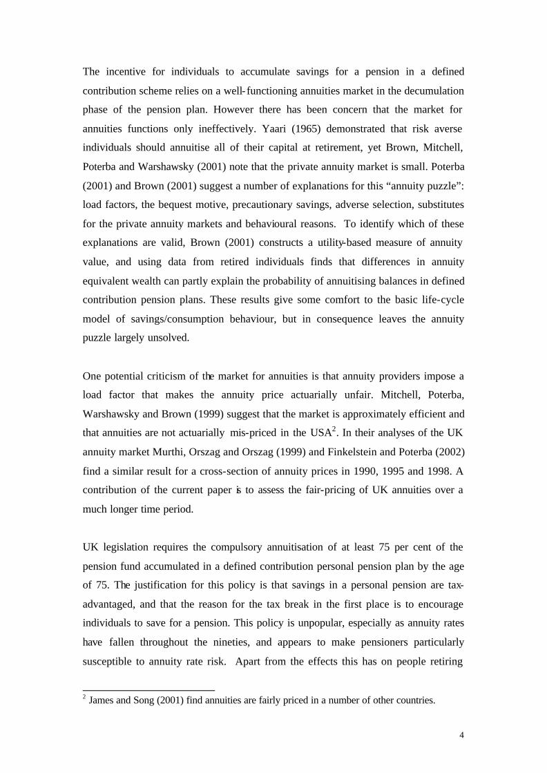
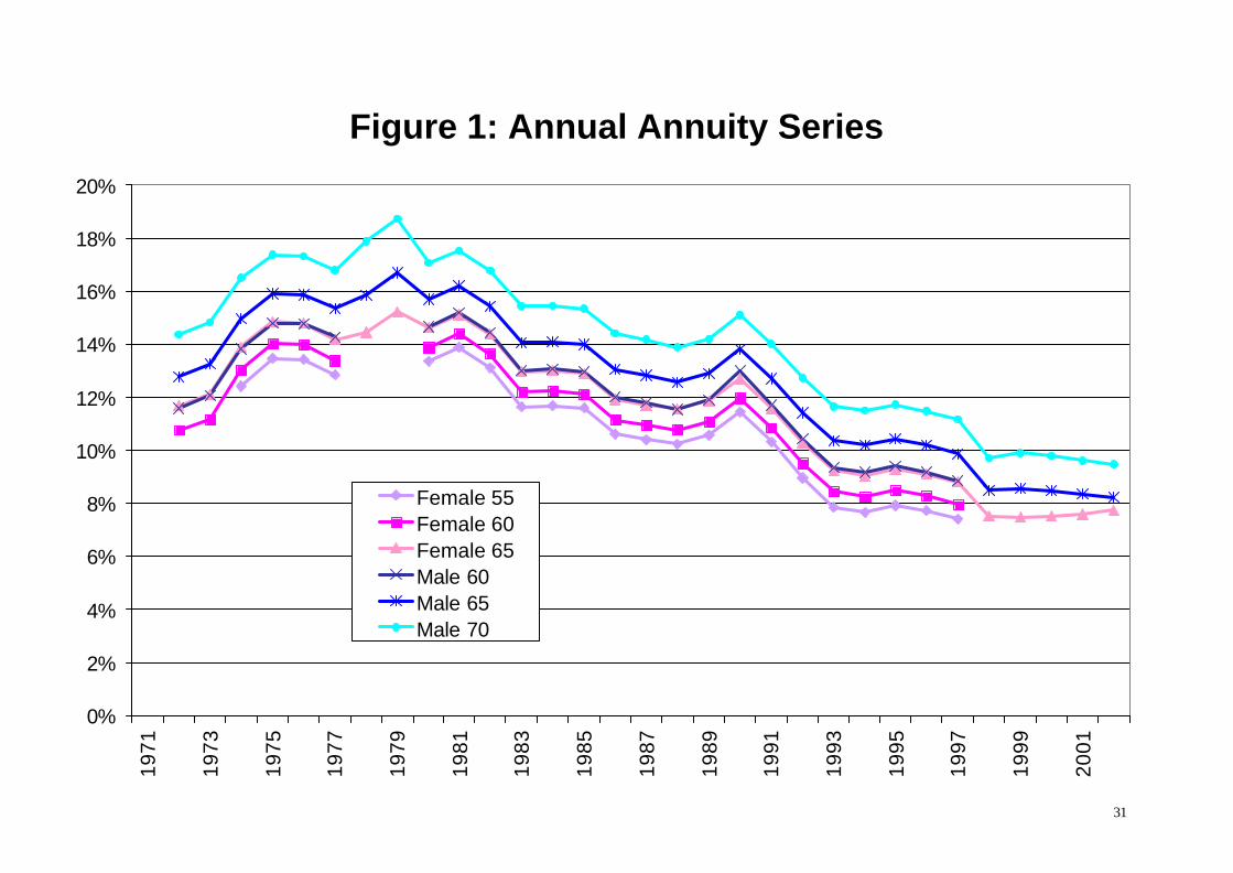
Figure 1 plots a series of 5-year guaranteed annuity rates for men aged 60, 65 and 70,
and for women aged 55, 60 and 65, over the period 1972 to 2002. It can be seen that
annuity rates for men are consistently higher than for women of the same age; and that
annuity rates are higher for both men and women as age increases. Age and sex are
two personal characteristics that annuity-providers condition on when quoting annuity
prices, since life expectancy of women is higher than men, and of younger adults of
both sexes is higher than older adults. The striking aspect of Figure 1 is the extent to
which the six series move together. In our subsequent work we will, therefore,
concentrate on the annuity rates of 65-year old men.
III Comparison of Annuity Rates with Long-term Interest Rates
Our data over the entire sample period are illustrated in Figure 2. For comparison with
other interest rates we also plot the consol rate. Theoretically these two series should
be linked because they are both long-term assets: if longevity were constant and the
short term rate were not particularly variable then the two would differ on average
only by a constant.
Descriptive statistics are presented in Table 1 for the two sub-periods and also for the
period as a whole (the annuity series for 1957 to 2002 created by splicing the series
together). As can be seen from Figure 2, the series are highly correlated and the
difference between them is falling over time. Both series appear to follow a unit root
process and so we considered whether they are cointegrated. Roughly speaking,
annuity rates are the consol rate plus a premium based on life expectancy and
10
although the last is trending down, probably with a unit root itself, it is sufficiently
slow moving and low variance compared with interest rates that it is unlikely to affect
the cointegration properties of the series on this relatively short time series. However,
any rejection of a unit root in the difference between the two series would have to be
very tentative: the conclusions of augmented Dickey-Fuller tests are sensitive to the
precise form of the test, the number of lags in the analysis and the sample period
chosen.
We conclude that annuity rates and consol rates are clearly highly correlated, but that
the precise nature of the relationship between the two is more complicated than a
simple cointegrating relationship.
IV Net Present Value Calculations
There are two ways to compare the value of annuities with other assets. One method
to calculate the value of an annuity is to use the measure called the “money’s worth”,
which is the ratio of the expected present value of the flow of payments made by an
annuity to the money paid for an annuity. This procedure has been used by Mitchell et
al (1999) to analyse the annuities market in the USA and by Murthi, Orszag and
Orszag (1999) and Finkelstein and Poterba (2002) to analyse the UK annuity market.
The last two papers are similar: the former has some information on UK annuity rates
at different points in time and the latter considers the variation between different
annuity providers and products. For a general discussion of the calculation of the
money’s worth see the introduction to the collection of papers in Brown et al (2001).
The alternative way to compare the value of annuities with other assets is to consider
the internal rate of return implied by an annuity rate. The advantage of the latter
approach is that it is necessary only to project life expectancies, whereas the money’s
worth approach requires assumptions about expectations of future interest rates as
well. Our results, however, are sufficiently similar that we do not report them here.
Returning to the money’s worth approach: define the annuity rate At as the payment
made per year of an annuity that cost £1 to buy in year t. The money’s worth for a
level 5-year guaranteed annuity can be written as
11
(1) ( ) ( )
+++ ∑ ∏∑∏∞
=
−
=
−+
=
−
=
−+
71
65
1
165,,
70
66
65
1
1 11k
k
jjtkt
k
k
jjtt rrA π
where rt+j is the interest rate in period t + j and π t,65,k is the probability of someone
born in year t - 65 surviving to age k having reached age 65.5 Note that the first five
years of payments for a 5-year guaranteed annuity is not affected by the survival
probability, since the annuity payments are paid out irrespective of whether the
annuitant dies in this period. For non-guaranteed annuities the money’s worth
calculation will involve the annuity payment multiplied by the survival probability
from the first year of the pay-out. Analogous formulae can be used to calculate the
money’s worth for annuitants at different ages, but the results are very similar for all
of the ages that we considered.
There are two ways to implement the calculation of equation (1), which we shall refer
to as ex ante and ex post. Our ex ante implementation uses expectations of interest
rates and survival probabilities that were available at time t. We estimate expectations
of future interest rates from the term structure of interest rates. This means that the
1957 interest rates used to value an annuity sold in 1957 are the implicit rates in 1957
yield curve. Apart from consistency across time, the approach has the advantage that
it can be compared directly with Mitchell et al (1999), Murthi, Orszag and Orszag
(1991) and Finkelstein and Poterba (2002).
The term structure of interest rates is available on a detailed basis only from 1979
onwards (on the Bank of England’s web site). These data are constructed by fitting a
smooth curve through data points for rates of return on government stock of different
maturities. However, the current published series were only calculated in 1999 and so
much of them were not available contemporaneously. Up to 1966, published yield
curve data in Financial Statistics was based not on a curve fitted to data but on
5 This appears to assume that no (fraudulent) payments are made to the annuitant or his or her estate after the point of death (disregarding payments made in the guaranteed five years period). Evidence from the Audit Commission (2002) suggests that such fraud may not be insignificant: £24 million of fraudulent payments were discovered for 2000, despite relatively few pensions providers taking part. Since our mortality statistics are presumably based on death as perceived by the life office (i.e., when it stops making the payments, regardless of when death actually occurred), our money’s worth calculations will be unaffected.
12
representative securities and described simply as “short-dated” (4 years), “medium-
dated” (8-10 years) and “long-dated” (15-25 years): these series were replaced in
Financial Statistics: after 1966, these series were replaced by the inferred rates of
return at 5, 10 and 20 years, themselves calculated using a different algorithm (we
have been unable to reproduce this). Most of our analysis is based on these published
data in Financial Statistics augmented by series SNPY, MNPY and LNPY from 1970,
with rates of return at intermediate maturities inferred by interpolation. We have also
used the current Bank of England series for 1979-2002 and compared the results as a
robustness check on our interpolation: the results were very similar.
It is, of course, well known that the term structure is rather a mediocre predictor of
future interest rates. According to theories where there is a liquidity or term premium
or according to preferred habitat theories, it may be a biased predictor. Most
discussion assumes that longer rates are higher because of a term premium, in which
case the interest rates we infer from the yield curve (at the long end) will be biased
upwards and the money’s worth biased downwards. Since we shall be arguing that
the money’s worth is quite high, this bias will be against our argument and in fact
strengthen our conclusions.
As mentioned in the Introduction, however, there may be some reason to believe that
long term interest rates are currently biased downwards, in which case we would be
over-estimating the money’s worth. We shall partially address this problem both by
considering ex post estimates of the money’s worth and also in the following section
where we discuss the value of pensions.
Obtaining expectations of mortality is more complicated. In particular we need to
know mortality of voluntary immediate annuitants, since there is clear evidence that
the mortality experience of such individuals differs both from other pensioners and
the population as a whole (see Finkelstein and Poterba, 2002, for a discussion of this
issue). To calculate ex ante survival probabilities we used the last published actuarial
projected life tables for each year. These are currently published by the Continuous
Mortality Investigation Committee of the two actuarial professional organisations in
the UK (the (English) Institute of Actuaries and the (Scottish) Faculty of Actuaries).
A census of life offices is taken every four years and the aggregate data published
13
with a lag of between three and five years, the delay presumably being due to the time
taken to collect the data in a satisfactory format. On a less regular basis, CMIC
publishes a statistical analysis of the data and proposes new standard tables which
include projections of future improvements in mortality. For the period in which we
are interested the relevant standard tables (including future projections) are given in
table 2.
It might seem surprising that the tables are up-dated so infrequently and this
infrequency might prompt doubts as to whether life offices use these tables without
making further adjustments which would not be available to us. This problem is
particularly acute for the use of the a(55) table in the 1970s. However, there is
satisfactory evidence that this table was in use in 1970s: as interest rates rose in the
1970s supplements to the a(55) table containing monetary functions were published in
1971 and 1973 and CMIR 5 (1981) suggests that a(55) was still used extensively in
1981, despite having been superceded by the a(90) table. CMIR 1 (1973), which
contained summary details of mortality experience up to the quadrennium 1967-1970,
showed that the a(55) projections of mortality fitted the actual data quite well and no
detailed statistical evidence was published until CMIR 2 (1976). It may be that no
life office would have had the ability to perform the detailed econometric analysis of
the CMIC anyway: given the small sample problems that occur at several points in the
analysis of the aggregate data, it is highly doubtful whether an individual office would
have had sufficient internal data for a meaningful analysis.6
These tables all contain estimates of the probability of dying at a given age, the
“mortality”, which we write as ktq +65, for someone aged 65 + k who was born in year t
- 65. In all of the tables a distinction is made between the probability of dying at a
given age in the year after purchasing an annuity (duration 0, sometimes referred to as
“select”), q0, and the probability of dying at a given age after a longer period of time
has elapsed (duration 1+, sometimes referred to as “ultimate”), q1+. The mortality at
duration 0 is lower than at duration 1+, presumably because agents have some
6 The Continuous Mortality Investigation Reports are concerned with a variety of actuarial analysis of which immedia te annuities are only a small and diminishing part, eg in 1979-1982, the numbers of Male and Female policies (“Exposed to Risk”) for annuities were 67 thousand
14
information over their chances of dying and can choose not to buy an annuity if the
chances of dying in the near future are high: this is a typical selection effect, although
since the information is also known to the life offices there need be no issue of
adverse selection through asymmetric information. In some of the CMI Reports
further distinctions are made between durations 1-4 and 5+ but the overall picture is
rather confused and we do not make much use of this information either here or later.
We calculate the survival probabilities by the formulae:
( ) 11
,1
65,165,1
65,65,65,
065,65,66,
>−=
−=
−++
++ kq
q
ktktkt
tt
ππ
π
Finkelstein and Poterba (2002) calculate the money’s worth using two sets of
mortality statistics: one based on “Lives” (IML), calculated as a simple average of
mortality experience and one based on “Amounts” (IMA), calculated as a weighted
average of mortality experience where the weights are the size of the policy. Because
of selection and socio-economic effects, we should expect the money’s worth
calculated on Lives mortality to be lower, which is borne out in the analysis of both
Finkelstein and Poterba (2002) and ourselves. Unfortunately the mortality statistics
for immediate annuitants were not published on both bases until the 92 tables and so
we are unable to make this comparison before 1999: all previous analysis is on the
basis of Lives alone.
In addition to the ex ante estimates of the money’s worth we also calculate ex post
money’s worth using the actual one-year interest rate and actual mortality experiences
of annuitants.7 Of course we do not know these data for years after 2002 (in fact we
do not know the mortality data after 1998 – these data for the quadrennium 1999-2002
will presumably not be published until 2004 at the earliest), so our calculations are not
and 151 thousand respectively compared to the total numbers of all pension policies of 5,244 thousand and 987 thousand. 7 The data on actual mortality experiences at duration 1+ is available annually for 1983 to 1998 in CMIR 19 (2000) and for 1975 to 1982 in CMIR 8 (1986). In both cases the data is expressed in the form of a ratio of actual mortality to expected mortality where the latter is taken from the respectively from the 92 standard tables (which can be found in CMIR 12, 1999) and the a(90) standard tables. For duration 0, we were unable to use annual data because it had not been published and even the quadrennial data was based upon a very small
15
really ex post for the whole period: for 1992 the proportion of the money’s worth for a
Male aged 65 based on actual data is approximately 75 per cent and that on estimates
is the remaining 25 per cent. Of course ex post the proportion is larger for earlier
years.
The ex ante money's worth is illustrated in Figure 3. The observations for 2001 and
2002 are not perfectly comparable with previous years, since not all of the relevant
mortality data is available, and not all of the yield curve data is yet published: the
2002 observation is based on the first quarter only. Over time there have been
considerable variations in the money’s worth, but it has remained within a band of 90
pence and 110 pence per £1. Both of the more recent revisions to the mortality
projections illustrated have shown increases in the money’s worth, i.e., actuaries
believe that they have underestimated increases in life expectancy. It is noteworthy,
however, that actuaries have not always under-estimated increases in longevity and
the improvements projected in the a(55) tables were not realised.8
This graph also suggests that the ex ante money’s worth is not particularly poor at the
moment. Certainly there have been times when it was worse, notably some of the
1970s. This is in addition to the problem of inflation: a fixed nominal payment was
worth less in the 1970s because it was more quickly eroded by the high inflation of
that period, something which will be inadequately accounted for by discounting with
the yield curve because it is well known that interest rates failed to fully incorporate
changes in inflation at that time.
Our attempts to estimate ex post money’s worth in Figure 4 also suggest that the
historical norm is for a value about £1. As discussed above, the most recent years of
this graph are not truly ex post, but the results are consistent with the ex ante results,
namely that the money’s worth has consistently been about unity.
number of observations, so we used the relevant base tables (without projection) which give the numbers arising from the graduations of the data. 8 These improvements (for both male and female mortality rates) were based upon the actual improvements in female annuitant mortality over the period 1880-1945: the data for male mortality over this period was too variable to be used for a projection. Note that the number
16
These results are very similar to the cross-sectional analysis of Finkelstein and
Poterba (2002) and Murthi, Orszag and Orszag (1999). The former found the
money’s worth to be 90 pence and the latter 93.2 pence in 1998, comparing with our
ex ante figure of 99 pence. Murthi, Orszag and Orszag (1999) also provide estimates
of 99.6 pence in 1990 and 92.1 pence in 1994: our analogous figures are 98 pence9
and 89 pence.
V Decomposition of Variability in the Money’s Worth
Despite the money’s worth being quite attractive, there is considerable year on year
variation. Since we know all of the determinants of the money’s worth, we can ask
what is causing this variation. The mean money’s worth is always close to unity, so the
standard deviation is approximately the same as the coefficient of variation and can be
interpreted as the percentage deviation from the mean
To implement this decomposition, we recalculated the means and standard deviations
holding some of the determinants of the money’s worth constant for the whole period,
replacing the time series with the mean of observations over the period 1972 to 2002.
Since the money’s worth is stationary, this will provide a reasonable description of the
underlying causes of the variability.10 Our results are shown in the Table 4.
The three determinants of the money’s worth are the annuity rate, the yield curve and
mortality.11 Holding either the yield curve or the annuity rate constant on their own
leads to a much larger standard deviation in the money’s worth, in the region of 20
pence, but this is misleading since we have already seen that interest rates (at least at
high maturities) and annuity rates are highly correlated. Holding both the annuity rate
and the yield curve constant, the standard deviation falls from the actual figure of 5.8
pence to 2.8 pence.
of female annuities in force over that period was considerably larger than the number of male annuities. 9 The figure of 98 pence for 1990 is based upon the money’s worth calculated using the a(90) table. Using the IM80 table, which was just available in that year, the figure would be 103 pence. 10 This is with the caveat that the data underlying our money’s worth calculations are not stationary, or even stationary around a linear trend, as was shown above. 11 The data for the yield curve and the mortality are vectors for each time series observation, so we took the average of the vector, i.e.,
17
On the other hand we can consider the money’s worth using actual annuity rates and
yield curves and using a constant average mortality, but this makes virtually no
difference.12,13
We conclude that although interest rates and annuity rates are highly correlated, it is
largely through variations in these variables that the money’s worth has changed over
time and that changes in mortality have had only a minimal effect. An important
implication of this is that the timing of annuitisation taken in isolation does affect the
size of the pension income that an annuitant can obtain. However, there are two
problems with using this fact: first, choosing the timing of annuity purchase to
increase income would only be possible if changes in the money’s worth were
predictable and given the evidence in Figure 2, this is unlikely.14 Second, it is not
appropriate to consider the money’s worth in isolation, since changes in the money’s
worth might be offset by changes in the value of the assets (i.e., the pension fund) that
would be used to buy the annuity, an issue that we consider in the next section.
We have shown that using the money’s worth criterion, annuity rates appear
competitive compared with the last thirty years. This result depends to a considerable
extent on the yield curve being a valid source of information for the calculation of the
money’s worth. As we have noted, however, this may not be valid if, as would be the
case in preferred habitat theories, the long-term interest rate is itself artificially low:
the fact that there is efficient arbitrage between annuity markets and bond markets is
( ) ( )∑∑∑ =
=
−=
=
−=
=
−==Tt
t Nt
Tt
t t
Tt
t tN xTxTxTxxxx1
1
1 21
1 11
21 ,,,,, KK . 12 In fact we used constant survival probabilities rather than constant mortality q. 13 It might seem strange that holding mortality constant makes virtually no difference to the standard deviation, while holding interest and annuity rates constant only halves the standard deviation: the inferrence might be that there is some variation which is totally unexplained. The reason for this apparent anomaly is that if we calculate the money’s worth holding constant interest rates and annuity rates, then the resulting time series of money’s worths trends up over time (the variation about this trend is negligible). This is because (apparently) annuity rates do take account of improvements in mortality. To decompose the variation of the money’s worth more precisely we should need to take account of the trending nature of mortality: given the relatively small number of time series observations and the magnitude of improvements in life expectancy over this period, this did not seem worthwhile. 14 A first order autoregression of the money’s worth over the period yields an R2 of 0.022 and an equation standard error of 0.059: the coefficient on the lagged dependent variable is 0.150
18
of little comfort if all financial markets are distorted. We address this question
indirectly in the next section by asking how much pension an annuity can buy at the
present time.
VI Value of Pension Funds
The previous discussion centred on the actuarial fairness of annuity contracts.
Perhaps more important to the actual annuitant is the pension that he receives,
regardless of how long he lives. This means that we need to consider both the
accumulation phase (building up the fund) and decumulation phase (buying the
annuity) together. The value of the pension received by a pensioner is AV, where A is
the annuity rate and V is the value of the pension fund at the point of retirement
(assuming that all of the pension fund is annuitised). It is a well-known empirical
regularity that the value of assets is negatively correlated with interest rates. This is
theoretically unsurprising, since the formula for the value (strictly speaking net
present value) of an asset is negatively related to the discount rate. Thus there is very
good reason to believe a priori that the variables A and V will be negatively
correlated. If this is so then any discussion of pensions needs to address the
relationship between these two variables, since A may form a partial hedge against
changes in V.
To do this we need to determine how the value of individuals' pension funds have
changed over time. Since we have no data on the value of pension funds, we construct
the pension funds of a series of hypothetical individuals who save according to a well-
specified rules and use these to calculate the resulting pension.
Diamond (1977) introduces the concept of a pension “replacement ratio”, defined as
the ratio of the pension income to labour income (net of pension contributions) in the
final year of employment. If the savings rate is 10 per cent and pension income is 60
per cent of labour income, then the pension replacement ratio is 60/90 = 2/3 and
Diamond suggests that this replacement ratio might be appropriate. Empirically such
replacement ratios are common in UK company pension schemes where employees
have completed their full set of contributions.
(statistically insignificant at the 10 per cent level). This confirms the prima facie evidence of
19
The optimal value of the pension replacement ratio is unclear. In a simple utility
maximisation framework where agents only wish to smooth consumption flows, the
optimal ratio would be one. However, this result does not follow if agents also obtain
utility from leisure and utility is not additively separable in consumption and leisure:
because leisure discontinuously increases at the point of retirement we should also
expect consumption to discontinuously fall. We might note that there are at least two
reasons for consumers’ expenditure to change upon retirement: the elimination of
work-related expenditure (commuting etc) and variation in expenditure on leisure
activities. Some of these expenditures may be discrete rather than continuous choice
variables (especially commuting) and hence provide a further reason for discontinuity
at the point of retirement.15
Consider the pension fund of someone retiring at time t, who has contributed a
proportion s of their income yt-i in year it − to a fund for the last R years. Each year
jt − the entire value of the fund (including previous years’ returns which are re-
invested) earns a rate of return jtr − . Then the value of the fund at retirement at time t
is
( ) ( ).1/10
1
0∏∑
=−
−
=− ++
i
jtjt
R
iit rrys
(We assume that no return is earned on the last year's contribution.)
To get some feel for the size of the figures, we consider first a very simple example
known as the “60:40:20:10:5:2 rule”: this will provide a rough and ready benchmark.
With a constant rate of return r and with constant income growth so that
( )ss gyy += 10 , the formula for the value of the fund at retirement simplifies to
Figure 2 that any attempt to predict the money’s worth would require additional information. 15 Banks, Blundell and Tanner (1998) show that there is a fall in actual consumption upon retirement and argue that it cannot be fully explained within a utility maximising framework unless there is unexpected adverse information at the point of retirement. Demery and Duck (2001) suggest that some, although not all, of the apparent problems in reconciling income and consumption data with the life cycle hypothesis of consumption may be due to selection effects and problems in appropriately mis-measuring pension income.
20
( ) ( ) .111
0
10∑
−
=
−+− ++R
i
iRit rgys
This fund can then be converted into an annuity over the expected retirement life of
the individual. Now make the following assumptions:
• the agent works and saves towards the pension for 40 years;
• the agent will be retired for exactly 20 years;
• while working and contributing to the pension fund the contribution rate is 10 per
cent;
• the rate of return on both savings during the accumulation and decumulation
phases (i.e., while building up the pension fund and on purchasing the annuity) is
5 per cent;
• real wages grow at 2 per cent per year while the agent is working;
• the agent buys a level annuity.
While it is not suggested that any of these assumptions are true for any particular
cohort of savers, they are clearly a reasonable approximation to reality. 16 Perhaps
surprisingly, the pension that results is almost exactly 60 per cent of final gross
income and hence the replacement ratio is 2/3.
Rather than assume a constant rate of return and labour income growth, we use actual
data to calculate possible pension fund values. We consider a series of hypothetical
individuals whose labour income is proportional to the UK average earnings index in
each year of their life.17 The average earnings figures were taken from the
16 An additional consideration is the rôle of taxation. By ignoring taxation we are clearly doing an “as if” simulation, where tax rules are basically the same as existing tax regulations, although this was not, in fact, the case for all years after 1918. It is also true that someone who did make use of these rules might have purchased a pension scheme different from an immediate annuity. However, given the complexity of the tax structure for much of the period (with highly progressive rates of taxation), any simulation would need to be based upon additional assumptions about the proportions of earnings and income which were taxed at different rates, which is beyond the scope of the present paper. 17 Earnings actually vary systematically with age, but unfortunately we do not know of any panel data on earnings by age cohort (we should need data back to about 1920) certainly there is none in the British Labour Statistics Historical Abstract or Chapman’s analysis of wages and salaries over the period 1920-1938. In the absence of such data we have conducted an
21
government published series LNMM from 1963 onwards. Data for earlier years are
taken from Mitchell (1988, pp.171-178), itself drawn from British Labour Statistics
Historical Abstract (1973) and Chapman (1953).
From the age of 26 to 65, the representative individual saves 10 per cent of their
labour income and invest it in some combination of bonds and equity: all returns are
re-invested. To account for charges, we assume that there is a 5 per cent charge for
purchasing shares, so that the effective savings rate is 9.5 per cent instead of 10 per
cent, that there is a 2 per cent charge every year on the equity investments and 1 per
cent per year on bonds, and that the spread is zero. These charges are consistent with
the estimates of charges found by Chapman (1999). At 65 the agents purchase an
annuity at the prevailing annuity rate.
We consider three different investment rules:
1. Invest entirely in equity;
2. Invest half in equity and half in bonds;
3. Invest everything in equity for the first 28 years of saving. Over the next
nine years, gradually reduce the proportion in equity and increase the
proportion in bonds until everything is in bonds for the last three years.
This type of investment scheme is sometimes referred to as a “life-style”
scheme
The life-style suggested rule approximates to the suggested rule of many fund
managers, who argue that it is too risky to hold equity towards the end of the
accumulation phase.
Figure 5 shows the replacement ratio under these assumptions. The three graphs
show the replacement ratios for a series of individuals who have invested their savings
in different portfolios of bonds and equity. So the observations in 1957 are for agents
who started saving in 1918 and retired in 1957; the observations for 1958 are for
analysis assuming that the profile of age-specific earnings relative to the average was constant over the whole period using estimates for the 1990s alone using estimates from Miles (1997), but the results were very similar to the ones with no allowance for age specific earnings.
22
different agents who started saving in 1919 and retired in 1958 (and thus faced
different wages and rates of return for some of their life.
These replacement ratios for much of the period lie between 0.4 and unity, with low
replacement ratios in the early part of the sample mainly because bond returns were
poor. The best strategy was clearly to invest in equity, which earned higher returns,
even for most of the 1970s. Only in the last few years have portfolios using bonds
been better: although switching out of equity into bonds meant that such portfolios did
not benefit from the stock market bubble of the late ‘nineties, they did benefit from
the large increases in the value of bonds as interest rates fell.
It is clear from the graph that the last two years have been less favourable times to
retire than the late 1990s: the last year would also look worse if we had data for more
than the first quarter of 2002. But the overwhelming message is that the fall in
replacement ratios is largely due to a return to more historical values. The period of
the last five years were actually characterised by high replacement ratios. The worst
year to retire was certainly 1974, when annuity rates were relatively high, but the
stock market had crashed.
It should also be noted that the steady increase in replacement ratios since 1974 is
despite increases in longevity over the last 30 years, which is ignored in this section.
Thus individuals retiring in 2002 on the same replacement ratio as people 30 years
earlier are better off, since they live longer and have a similar or better annual income.
23
VII Simulations of Replacement Ratios
So far we have calculated replacement ratios from a series of hypothetical individuals
retiring between 1972 and 2002. We now discuss whether we can use empirical data
to say more about replacement ratios. As we have seen in Figure 2, the annuity rate
behaves very similarly to the consol rate and we could safely model the annuity rate
as the consol rate plus a constant -- in this case 3.21 per cent which is the mean
difference over the latter period for which we have data. Having made this assumption
about the relationship between the consol rate and the annuity rate, it would be
possible to calculate replacement ratio for someone retiring in the last few years so
long as we had just three data series: the equity yield, the consol rate and earnings.
Using data for 1918 to 2000, we estimate the behaviour of the equity yield, the
logarithm of the consol rate (using logarithms ensures that this variable is never
negative) and the growth rate of earnings in a VAR with a constant but no trend.18 We
use this estimated relationship to conduct two types of simulation. First, we assume
that the residuals are normally distributed and use the estimated covariance matrix to
generate residuals; second we use a boot-strap style simulation where we randomly
sample (with replacement) from the empirical residuals. In each simulation we use
100,000 replications to calculate the density function of the replacement ratio. Our
results for the average of the three different forms of pension saving are shown in
table 5.
Unsurprisingly the replacement ratio is highest if the pension fund is invested entirely
in equity and lowest if invested in half equity and half bonds. Higher replacement
ratios, however, are not achieved costlessly: the equity portfolio has the highest risk
(measured in terms of standard deviation, not shown here) and the half-and-half
18 None of these variables are obviously trending over the period. Using the Akaike or Schwartz criteria alone we would have chosen only one lag in the VAR, but this model evidenced considerable residual autocorrelation, which was absent in models with two or three lags. Regardless of the number of lags used, there was overwhelming evidence of autoregressive heteroskedasticity and excess kurtosis in the residuals. The latter problem was dealt with individually by using empirical residuals (boot-strapping) in our simulation analysis. Both phenomena are more likely to be due to time-varying risk and a better solution would have been to model the data using a vector-ARCH process. However, to model a 2-lag VAR whose residuals were ARCH(1) would involve estimating about 50 parameters (depending upon the precise specification) and we had too few observations (80) for this to be a worthwhile exercise.
24
portfolio is the least risky. While we can be confident about the relative size of these
replacement ratios, the absolute size depends considerably upon which simulation is
used.
The deciles for the 3- lag VAR simulation using boot-strapped residuals are shown in
Table 6, and as a sensitivity test, deciles for the 2- lag VAR simulation using boot-
strapped residuals are shown in Table 7. Figure 6 shows the probability distributions
from the 3-lag VAR simulation. It can be seen that the equity:bond portfolio
investment strategy appears to dominate the other two. In fact we were not able to
demonstrate that any investment strategy stochastically dominated any other, because
at low values of the pension replacement ratio the values for the alternative strategies
intersect. Although for each strategy there is significant upside potential, according to
Table 6 there is a ten per cent probability of getting a replacement ration of less than
thirty per cent. Tables 6 and 7 demonstrate that the shape of the pension replacement
ratio distributions are similar whichever model for generating the simulated data is
used.
VIII Conclusions
In this paper we have constructed a time series of purchased life annuity prices since
1957. This is considerably longer than the only other time series for UK annuities
that we know to have been published in Murthi, Orszag and Orszag (1999) which
included a graph of the best annuity rate for the period 1988-98.
Using this series we are able to answer a number of questions. First, are annuity rates
unfairly low? Second, how much pension income have individuals been able to
generate? Third what is the risk inherent in a defined contribution pension scheme?
In answer to the first question we find no evidence that the average annuity rate in the
UK over the period 1957-2002 has been unfairly low. Depending on the assumptions
we make about future longevity, the present value of an annuity is of the order of
between 90 per cent and 100 per cent of the purchase price. Compared with the
typical costs of buying financial services this figure looks suspiciously good: annuity
providers must earn a profit and cover the real resource costs of annuity provision. It
is possible to turn the question of low annuity rates on its head: are in fact annuity
25
rates too high? James and Song (2001) argue that in fact life insurers may be able to
earn a higher rate of return than the riskless rate that we have assumed from the term
structure and hence such money’s worths are consistent with annuity providers
making profits and covering resource costs.
A possible response to this conclusion is that current annuity rates may appear to
provide a good money’s worth because the latter is calculated using interest rates
which are themselves distorted.
In answer to our second question, we find no reason to suggest that individuals are
worse off by annuity rates being low, since this has been off-set by increases in the
value of pension funds over the last forty five years. Even apart from the fact that
people retiring today expect to live longer, their pension income (compared to their
final salary) looks as good as ever.
Finally we have simulated financial market data and calculated pension replacement
ratios for a large number of independent economies to build up a frequency
distribution of the replacement ratio that would be faced by individuals saving
through a defined contribution pension plan. We find that the median pension
replacement ratio generated by a typical savings plan of 10 per cent of salary saved
over 40 years lies between 60 and 100 per cent. Within this distribution there is a lot
of upside potential, but there is a ten per cent probability of getting a pension that is
less than 30 per cent of salary.
26
Table 1: Time Series Properties on Annuity and Consol Rates
Mean 12.1 8.57 3.53 St.Dev. 2.39 2.90 0.96 Correlation 0.95
Table 1 presents descriptive statistics on the time series of average annuity rates and consol rates over the period 1957 to 2002 and for the two sub-periods.
Table 2: Data used by Continuous Mortality Investigation Committee of the
actuarial professional organisations in the UK to calculate life tables
Name of Table Date Table
published
Possible dates
Table used
Data used to construct the Table
a(55) 1953 1953-1978 1946-1948
(a90) 1978 1978-1990 up to quadrennium of 1971-1974
IM/IF80 1990 1990-1999 up to quadrennium of 1979-1982
IML/IMA/
IFL/IFA92
1999 1999- up to quadrennium of1991-1994
Table 2 lists the dates of the published actuarial projected life tables for each year, produced by the Continuous Mortality Investigation Committee of the two actuarial professional organisations in the UK (the (English) Institute of Actuaries and the (Scottish) Faculty of Actuaries). The CMIC publishes a statistical analysis of the data and proposes new standard tables which include projections of future improvements in mortality.
27
Table 3: Money’s Worth of UK Annuities 1957-2002
Years Type of Annuity
CMIC Actuarial Table Mean MW 95% confidence interval
t-test: p-value
lower upper 2-tailed test
1955-1973 no g'tee a(55) 1.0338 1.0013 1.0664 0.0423 1972-2002 5-year g'tee various 0.9852 0.9627 1.0076 0.1867 1972-1980 5-year g'tee a(55) 1.0040 0.9415 1.0664 0.8873 1978-1991 5-year g'tee a(90) 0.9778 0.9545 1.0010 0.0597 1990-1999 5-year g'tee IM80 0.9854 0.9543 1.0165 0.3159 1990-2002 5-year g'tee IM80 0.9764 0.9512 1.0016 0.0640 Table computes money’s worth over different sub-samples of the dataset and evaluates whether mean money’s worth is significantly different from unity.
Table 4: Decomposition of variability in the Money’s Worth: 1957-2002 Mortality Actual Actual Actual Actual Average Annuity Rate
Actual Average Actual Average Actual
Yield Curve Actual Actual Average Average Actual
Mean 0.973 1.017 0.971 0.976 0.973 Standard Deviation
0.058 0.225 0.191 0.028 0.058
Table decomposes changes in the money’s worth due to changes in mortality, annuity rates, and interest rates. Table 5: Simulated Replacement Ratios for Different Investment Styles Mean of Replacement Ratio All Equity Half Equity, half
bonds Life-style
Panel A: Normal errors 1 lag in VAR 1.720 0.864 1.273 2 lags in VAR 1.603 0.841 1.225 3 lags in VAR 1.449 0.764 1.106 Panel B: Boot-strapped errors 1 lag in VAR 1.487 0.842 1.152 2 lags in VAR 1.348 0.789 1.064 3 lags in VAR 1.243 0.710 0.923 Table calculates pension replacement ratios for simulated data.
28
Table 6: Deciles for the 3-lag VAR simulation using boot-strapped residuals
Replacement Ratio Decile All Equity Half Equity, half bonds
Life-style
0.1 0.325 0.288 0.289
0.2 0.453 0.360 0.387
0.3 0.580 0.427 0.485
0.4 0.720 0.495 0.588
Median 0.883 0.571 0.706
0.6 1.081 0.662 0.854
0.7 1.349 0.779 1.046
0.8 1.746 0.948 1.333
0.9 2.509 1.258 1.888
Table reports deciles of the pension replacement ratios for simulated data from a 3-lag VAR simulation
Table 7: Deciles for the 2-lag VAR simulation using boot-strapped residuals
Replacement Ratio Decile All Equity Half Equity, half bonds
Life-style
0.1 0.321 0.295 0.292
0.2 0.458 0.376 0.399
0.3 0.593 0.450 0.504
0.4 0.743 0.531 0.619
Median 0.919 0.619 0.752
0.6 1.138 0.724 0.919
0.7 1.439 0.861 1.141
0.8 1.887 1.065 1.477
0.9 2.509 1.258 1.888
Table reports deciles of the pension replacement ratios for simulated data from a 2-lag VAR simulation
29
References
Audit Commission (2002) Match Winner: Report of the 2000 National Fraud Initiative. Banks, James, Blundell, Richard, and Tanner, Sarah (1998) “Is there a Retirement-Savings Puzzle?” American Economic Review, 88(4), pp. 769-788. Blundell, Richard and Stoker, Thomas M. (1999) “Consumption and the timing of income risk,” European Economic Review, 43, pp. 475-507. British Labour Statistics Historical Abstract (1973) Brown, Jeffrey R., (2001) “Private pensions, mortality risk, and the decision to annuitize”, Journal of Public Economics, vol. 82, 29-62. Brown, Jeffrey R., Mitchell, Olivia S., Poterba, James M. and Warshawsky, Mark J. (2001) The Role of Annuity Markets in Financing Retirement (Cambridge: MIT Press). Cannon, Edmund and Tonks, Ian (2003) “The Construction of UK Annuity Price Series 1957 to 2002,” University of Bristol, mimeo. Chapman, Agatha (1953) Wages and salaries in the United Kingdom, 1920-1938 (Cambridge University Press). Chapman, John (1999) “Persistency and charges: exposing the big hitters,” Money Management, pp. 72-75. Craig, John (1998) “To be or not to be - what are the odds?” Population Trends, 92, pp. 42-50. Demery, David, and Duck, Nigel W. (2001) “Savings Age Profiles in the UK,” University of Bristol Working Paper, 01/518. Department for Work and Pensions and Inland Revenue "Modernising Annuities: A Consultative Document", February 2002. Diamond, Peter A. (1977) “A Framework for Social Security Analysis,” Journal of Public Economics, 8, pp. 275-298. Finkelstein, Amy and Poterba, James M. (2002) “Selection Effects in the United Kingdom Individual Annuities Market,” Economic Journal, 112(476), pp. 28-50. James, E. (1997) “New Systems for Old Age” World Bank, Working Paper James, E. and Song Xue (2001) “Annuity Markets Around the World: Money’s Worth and Risk Intermediation” CeRP Working Paper 16/01.
30
Miles, David (1997) “A Household Level Study of the Determinants of Income and Consumption,” Economic Journal, 107(404), pp. 1-26. Miles, D. and A. Timmerman (1999) “Costing pension reform: Risk sharing and transition costs in the reform of pension systems in Europe”, Economic Policy, 253-286 Mitchell, Brian R. (1988) British Historical Statistics (Cambridge University Press). Mitchell, Olivia S., Poterba, James M., Warshawsky, Mark J. and Brown Jeffrey R. (1999) “New Evidence on the Money’s Worth of Individual Annuities,” American Economic Review, 89, pp. 1299-1318. This article is reprinted in Brown et al (2001). Murthi, Mamta, Orszag, J.Michael and Orszag, Peter R. (1999) “The Value for Money of Annuities in the UK: Theory, Experience and Policy,” Birkbeck College, London. Discussion Paper. Poterba, J. M. (2001) “Annuity Markets and Retirement Security”, Fiscal Studies vol. 22, no. 3, 249-270 Poterba, J.M., S.F. Venti and D.A. Wise (1998), “401(k) plans and future patterns of retirement savings”, American Economic Review, vol. 88, no. 2, 179-184 Stark, J. (2002) “Annuities: the consumer experience”, ABI Research Report, (ISBN 1-903193-22-2) Warshawsky, Mark J. (1988) “Private Annuity Markets in the United States: 1919-1984,” Journal of Risk and Insurance, 55 (3), pp. 518-528. This article is reprinted in Brown et al (2001) Yaari, M. (1965) “Uncertain lifetime, life assurance, and the theory of the consumer”, Review of Economic Studies, vol. 32, no. 2, 137-50.
31
Figure 1: Annual Annuity Series
0%
2%
4%
6%
8%
10%
12%
14%
16%
18%
20%
1971
1973
1975
1977
1979
1981
1983
1985
1987
1989
1991
1993
1995
1997
1999
2001
Female 55Female 60Female 65Male 60Male 65Male 70
32
Figure 2: Annuity Rate, Male 65, level
0%
2%
4%
6%
8%
10%
12%
14%
16%
18%19
56
1958
1960
1962
1964
1966
1968
1970
1972
1974
1976
1978
1980
1982
1984
1986
1988
1990
1992
1994
1996
1998
2000
2002
q1
Mean annuity rate, gtd 5 years, no stale prices
Consols (2½% until 1992, then 3½% War loan)
Median Annuity Rate, no gtee
33
Figure 3: Money's Worth (Male 65)Contemporary ex ante estimates
0
0.2
0.4
0.6
0.8
1
1.2
1.4
1957
1959
1961
1963
1965
1967
1969
1971
1973
1975
1977
1979
1981
1983
1985
1987
1989
1991
1993
1995
1997
1999
2001
a(55)a(90)IM80IMA92IML92a(55) no guarantee
34
Figure 4: "Ex Post" Money's Worth Level Annuities, Male 65
0
0.2
0.4
0.6
0.8
1
1.2
1.4
1957
1959
1961
1963
1965
1967
1969
1971
1973
1975
1977
1979
1981
1983
1985
1987
1989
1991
1993
1995
1997
1999
2001
Guaranteed 5 years
No guarantee
35
Figure 5: Replacement RatiosDifferent portfolios of bonds and equity
0.0
0.2
0.4
0.6
0.8
1.0
1.2
1.4
1.6
1.8
2.0
1957
1959
1961
1963
1965
1967
1969
1971
1973
1975
1977
1979
1981
1983
1985
1987
1989
1991
1993
1995
1997
1999
2001
Half Bonds and Half EquityLifestyleEquityHalf Bonds and Half Equity (no g'tee)Lifestyle (no g'tee)Equity (no g'tee)