Probing Metal Nanoparticles and Assemblies with Analytical Ultracentrifugation MASS by Randy Carney Submitted to the Department of Materials Science and Engineering in partial fulfillment of the requirements for the degree of Science Masters in Materials Science and Engineering at the MASSACHUSETTS INSTITUTE OF TECHNOLOGY May 2010 C 2010 Massachusetts Institute of Technology All rights reserved Author ............... Certified by........ Accepted by.................... Chairm Department of at ' s Science and Engineering May 10, 2010 . ....................... ........... Francesco Stellacci ssociate Professor }}esis Supervisor ....... - ... s .. ... .... ...... Vristine Ortiz an, Departmental Committee on Graduate Students ACHUSETTS INST1TUTE OF TECHNOLOGY JUN 16 2010 LIBRARIES ARCHIVES
Transcript
Probing Metal Nanoparticles and Assemblies with AnalyticalUltracentrifugation MASS
byRandy Carney
Submitted to the Department of Materials Science and Engineeringin partial fulfillment of the requirements for the degree of
Science Masters in Materials Science and Engineering
at the
MASSACHUSETTS INSTITUTE OF TECHNOLOGY
May 2010
C 2010 Massachusetts Institute of TechnologyAll rights reserved
Author ...............
Certified by........
Accepted by....................
Chairm
Department of at ' s Science and EngineeringMay 10, 2010
AbstractAnalytical Ultracentrifugation (AUC) is a powerful tool to obtain statistically relevant sizeand shape measurements for macromolecular systems. Metal nanoparticles coated by a ligandshell of thiolated molecules provide diverse functionality, from targeted cellular delivery tothe formation of complex assemblies. Here I show that AUC can be used to determineparticle size distribution, ligand shell density, shape, and hydrodynamic radius. It can also beused to probe complex mixtures of nanoparticle assemblies, from 2D dimers and chains, to3D trimers, tetramers, and higher order assemblies, from a consideration of theirhydrodynamic shape factor and its relation to the sedimentation coefficient. With AUC, theease of sample preparation, ligand shell information, and dramatic increase in sample size areimprovements compared with electron microscopy, and the ability to probe multiple, discreteabsorbing wavelengths and globally analyze with interference information offers a measuredimprovement compared with dynamic light scattering (DLS). This work describes multiplecalibrations and considerations as well as theoretical contributions concerning the applicationof AUC to nanoparticle systems
Contents
1 Background1.1 Analytical Ultracentrifugation
1.1.1 Theory1.1.2 Instrumentation1.1.3 Principles of Sedimentation Velocity1.1.4 Lamm Equation modeling1.1.5 Microheterogeneity in Sedimentation Coefficient
1.2 Metal Nanoparticles1.2.1 Background1.2.2 Synthesis1.2.3 Assemblies
2 AUC Results2.1 Design of Experiments
2.1.1 Concentration2.1.2 Temperature2.1.3 Polydispersity, diffusion, and speed2.1.4 Radial Step Size
2.2 Particle Size Distribution2.2.1 c(s) model2.2.2 c(s, f/f0) 2D model
2.3 Assemblies2.3.1 Dimers2.3.2 Chains
3 Fractionation3.1 Experimental Procedure3.2 General Gradient Model
3.2.1 rband(s, W>, t)
3.2.2 Hydration Correction
Conclusion
Future Work
AppendicesAppendix A DerivationsAppendix B MATLAB code for c(s,f/fO) to c(ds,dD)
Bibliography
Chapter 1 BackgroundAs nanoparticles become a more viable option for applications in energy, biology, and
other complex fields , the importance of complete characterization increases. Typicalfeatures remain elusive in the field, such as sample purity, molar mass, sedimentationcoefficient, size and shape, stoichiometry, and binding affinity or kinetics, especially forcomplex assemblies of nanoparticles. Bulk sizing techniques such as electron microscopy(EM) and dynamic light scattering (DLS), and surface probing techniques such as atomicforce microscopy (AFM) and scanning transmission microscopy (STM), contain manyconstraints6, including technical limitations, steep complexity, and low statisticalsignificance. Most of these techniques don't allow the observation of the nanoparticles intheir native, biologically relevant state (e.g. suspended or in solution), with samples thatinstead must be immobilized on a surface and prepared with labels or tags. Still, thesetechniques are mostly unfit to directly measure many quantities associated with complexmacromolecular assemblies, let alone in a single measurement. For example, DLS might beused to measure size, but is limited to ranges above our group's nanoparticle diameter, orSTM may give surface information, but is too low in resolution to provide size.
In this thesis, I will use analytical ultracentrifugation, sometimes combined with bulkfractionation, to elucidate many quantities that are normally independently measured fornanoparticles (such as size and shape) from first principle and to higher resolution thancurrently avaliable without AUC. The objective of this thesis is to assist nanoparticlescientists to gain a greater understanding of AUC and to practically explain how modernsedimentation velocity experiments can be used to characterize nanoparticles andnanoparticle assemblies. Following this general treatment, I plan to examine how the surfacestructure influences the cell penetrating ability for a specific type of mixed-ligandnanoparticles.2
1.1 Analytical Ultracentrifugation
1.1.1 TheoryAnalytical Ultracentrifugation is a characterization technique popular in the fields of
molecular biology, biochemistry, and polymer science. A sample being spun experiencescentrifugal force, and the subsequent movement can be observed in real time with a set ofonboard optics, utilizing the sample's light absorption or optical refractive index differencesbetween the sample and solvent. Many sample features can be elucidated, including size,shape, and sample-sample interactions. Because this technique also fractionates the sample,we measure not only average values, but the compete distributions of these values, such asmolecular weight distributions (MWD), particle size distributions (PSD), and the densitydistribution (DD, chemical heterogeneity). Also, the polyelectrolyte character of dissolvedmacromolecules can be measured by multiple experiments using salt variation.As the sample is pelleted by centrifugation, the evolution of the sample concentration ismonitored and can be analyzed mathematically. The scope of the instrument involves twoprimary branches of experiments: sedimentation velocity (SV) and sedimentation equilibrium(SE) runs."'9
SV is a hydrodynamic method used to obtain size and shape information as determinedby mass transport from both sedimentation and diffusion, while SE is a thermodynamic
method that reports only on mass, not shape, which relies on allowing the diffusion flux andsedimentation flux to equilibrate (no net flux). In this work, only sedimentation velocity isconsidered, as the density of metal nanoparticles eliminates the possibility of balancingdiffusion and sedimentation, with sedimentation dominating. In general, SE and SVexperiments are used to characterize reversible protein interactions, such as self-association,heterogeneous association, multi-protein complexes, binding stoichiometry, and thedetermination of association constants. " Specifically, SV experiments are utilized todetermine sedimentation coefficients by analyzing the moving boundaries of sedimentingspecies. The information contained in the sedimentation coefficient is related to manyexperimental details by the Svedberg equation. Since the AUC measurement takes placewith molecules free in solution, the resulting size distribution is an accurate representation ofthe ensemble of particles in solution."
1.1.2 InstrumentationA centrifuge is an apparatus used to create centrifugal fields by fast rotation of a rotor;
ultra-centrifuges defined as a centrifuge capable of achieving more than -5000 times theacceleration due to the Earth's gravitation field (g). An analytical ultracentrifuge in anultracentrifuge fitted with one or several optical detection systems, allowing the observationof the fractionation process of a species dissolved in solution. Beckman-Coulter Instrumentsdeveloped two analytical ultracentrifuges, the XL-A and the XL-I, the former using UV andvisible absorption optics and the latter integrating absorbance and interference optics.13
Absorbance optics are capable of detecting single or multi-wavelengths andinterference optics detect small changes in refractive index between sample and solvent,which is useful for species which do not absorb, or absorb too poorly or abundantly at theconcentration of interest. By simultaneous multi-optical detection, complex colloidalsystems can be disentangled, even utilizing additional optical systems such as Schlieren, lightscattering, and fluorescence optics. 14 From an experimental standpoint, interference opticspresent disadvantages because refractive index variations are very sensitive to smallimpurities (high sample purity required), the optics must be independently adjusted beforeeach experiment, and greater care must be taken to match the volume and chemicalcomposition of the sample and reference cells (compared to absorbance). The choice of anappropriate optical detection system will be described in greater detail later. Because therotor speed can be varied over a large range (600-60,000 rpm) detectable molecular weightand diameter ranges are large (300<M<10 14 g/mol, 0.5<D<3000 nm), and SV runs typicallyrequire only 0.05 to 0.5 mg of material. Experimentally, small volumes (<450uL) of a dilutesolution containing the macromolecule is loaded into a special sector-shaped cell, beside areference cell containing only the naked solvent. The cells are loaded into one of twotitanium rotors (An-50/6OTi which hold 1-7 cells and a counterbalance used for delaycalibration of the optical systems) and the rotor is placed in a vacuum chamber at a controlledtemperature during centrifugation.
1.1.3 Principles of Sedimentation VelocityDissolved or dispersed samples are exposed to high gravitational fields induced by the
spinning of the centrifuge rotor, causing the solute macromolecules to drift from themeniscus to the bottom of centrifuge cell as a function of time. Each species is detected byoptical detection systems which measure the concentration change with time and radius,c(r,t). Consider a single spherical particle of mass m, and density Q, dissolved in a solvent(g) with density p, and viscosity q,, in a gravitational field wVr at a radial distance r from thecenter of rotation as in Figure 1 (adapted from [15]).
Figure 1: Forces on a centrifuging species
Three forces are immediately apparent.
The first is the centrifugal force Fe, induced by the acceleration wor of the AUC rotor:
2 2Fcent,fuga = m, 0 r = - r
N(Eq. 1.1)
where M is the solute molar mass and N is Avogadro's number. This is the only force actingaway from the center of rotation. Equation 1.1 illustrates that the centrifugal force increaseswith increasing mass of the particle, and thus larger particles sediment faster than smallerones (so long as the mass of the particle is greater than the mass of the solvent).
The second is the buoyant force F, governed by Archimedes principle and proportional tothe mass of the displaced solvent ms and wor, but opposite in direction to F.
F = - . 2 M _Fbuoyant = -ms' co2r = 2 - -.- c r (Eq. 1.2)
with v=( g,)- as the solute partial specific volume or the reciprocal of particle density.
The final is the frictional force F, produced by the movement of the particle through thesolvent, according to the hydrodynamic treatment of drag around an object:
with frictional coefficientf and the sedimentation velocity u of the solute.The three forces come into balance very quickly (~10-13 secs) after the application of a
centrifugal force and the particle achieves its terminal or sedimentation velocity u (theobserved velocity of the particle):
M. M _F +Ff =0=- ,- w 2r - f - u (Eq.1.4)
N N
By rearranging (Eq. 1-4):
- S (Eq.1.5)N- f w 2r
This contains the meaning of the sedimentation coefficient, s, now defined as theterminal velocity per centrifugal field. The frictional coefficient,f, is well known fromhydrodynamic theory, and depends on the shape and size of the particle. For a smooth,compact sphere under the Reynolds limit (small size), the Stokes-Einstein (Eq. 1.6) andStokes' equation (Eq 1.7) give f:
kT RTf- - (Eq.1.6)
D ND
f = 3,x- r,- d, (Eq. 1.7)
with Boltzmann constant k, gas constant R, and particle diameter d, of a spherical particle.
Merging Eq. 1.5 and Eq. 1.6 leads to the Svedberg equation:
M = s- p) (Eq 1.8)D(1 -;V,- pg)
now independent off (size and shape). Combining Eq. 1.7 and 1.8 gives the basis formeasuring Stokes-equivalent spherical diameters19:
18 - r,- sd, = _; (Eq 1.9)
The determination of s and its concentration in the sample are the primary outputs of theAUC.
1.1.4 Lamm Equation ModelingA more accurate thermodynamic approach to modeling particle sedimentation with
AUC utilizes the general Lamm equation, which describes the change in sampleconcentration with radius and time during an ultracentrifugation experiment. The partialdifferential Lamm equation describes the spatial and temporal behavior of concentration,considering mass transport of both sedimentation and diffusion. Diffusion describes thecooperative solute spreading effect produced by individual molecule Brownian motion. It
can be mathematically stated as a constant, the diffusion coefficient D, which is the spread ofthe molecule over time (units: cm2/sec). The diffusion and sedimentation can be separated,but contribute additively to the boundary shape, which is described fully by the generalLamm equation 5:
A solution is a spatially and temporally resolved concentration function, c(r,t). The AUCrecords the concentration (absorbance) profile by scanning (at up to three wavelengths ofinterest) at stepped intervals down in the radial direction down the cell. The mathematicalanalysis of the boundary movement of a species (with radius and time) allows theexperimental measurement of the diffusion and sedimentation coefficients. Figure 2illustrates the separation of the two terms for a single ideal species at a given time:
00sedimentation only -- +* + -with diffusion
Lamm Equation:
Radial distance from rotor center, r --
Figure 2: Centrifugal Mass Transport:- Sedimentation and DiffusionBottom: A step function solution accounting for the sedimentation (black), with the actual solution (red)considering diffusion, which causes significant boundary broadening. Top: a possible configuration of asingle ideal species in an AUC sector-shaped cell, which can be mathematically approximated by the red
solution to the Lamm equation below.
A single species (wholly defined by a sedimentation coefficient s) sediments as a singleboundary." The red concentration profile c(r) pictured in the lower panel of Figure 2 can betreated as a graphical solution to the Lamm equation for a given time. Computer software
(such as Sedfit, available from www.analyticalultracentrigation.com) can fit an array ofboundary profiles at different times to a set of experimental data points. The resulting c*(s)is a function that predicts an s-distribution and their relative concentrations (frequency). Theasterisk indicates that the distribution is of the apparent s-value, at a given temperature andsolvent condition. Generally, this is converted to the standard S20, value, by the followingthe equation15:
....... ................
nT ,g p - P20,0)S = ss. n,.(Pp - (Eq. 1.11)
20,w g $2,w p- PrT,)
The theoretical c*(s) fits the experimental data to user inputs of assumed values(solvent viscosity, density, solute partial specific volume, s range and resolution,regularization confidence, and frictional ratio). This is important, because AUC boundaryanalysis requires initial guesses that are close to the true values, therefore more independentmeasurements of these solution parameters will offer the best interpretation of theexperimental data. The software performs a least-squares regression to minimize the errorbetween the simulated solutions (generated in silico from the predicted c*(s) solution) andthe experimentally measured data points. The measure of fit, or 'rmsd,' can be used as ameasure to predict the validity of modeled solutions compared to the experimental data.
1.1.5 Microheterogeneity in Sedimentation CoefficientAt this point, the thermodynamic Lamm treatment has only been applied to a single,
ideal species. Consider two sedimenting species with separated s values from Figure 3:
s=3.5 S
s=7.0 S
Non-interactingspecies
s=3.S
s=45S
Non-interactingspecies
Radial distance from rotor center, r - Radial distance from rotor center. r -
Figure 3: Bimodal species(Left): The top and middle panels illustrate the two species measured separately, and the lower panel shows
the bi-stepped Lamm equation solution after superposition. (Right): Illustrating the resulting superposedboundary when considering a bimodal species close in s.
When the two species have separated sedimentation coefficients, two clear steps can beresolved in the combined boundary plot. They are normalized (height) by their relativeconcentrations in solution. The right panel illustrates the difficulty in resolving steps fordiscrete species that are close in s-value. Because diffusion also serves as a boundarybroadening effect, it becomes increasingly difficult to disentangle the sedimentationcoefficient, s, from the diffusion coefficient, D, as species are added to the solution."However, diffusion and sedimentation are two mass transport phenomena that occur ondifferent time scales, and at the limit of infinite time, sedimentation dominates.Experimentally one can increase the speed to simulate this effect, and in fact running thesame sample over a range of speeds can lead to a very accurate measurement of eachsedimentation coefficient, but at the expense of the diffusion coefficient. The general idea is
to deconvolute the effects of diffusion, so that it doesn't obscure the existence of multiplespecies, and then take diffusion into account to accurately predict other thermodynamicquantities such as hydrodynamic radius (RH), molar mass (M). The deviation of thehydrodynamic radius (measured from the experimentally fitted D)
While the analysis of sedimentation velocity experiments is straightforward and veryaccurate for s-monodisperse species, heterogeneity in s results in difficult complications thatshould be considered, namely that the s-heterogeneity is tough to distinguish from diffusion.Normally, the general c(s) is computed by the inversion of a Fredholm integral equation thathas Lamm equation solutions as kernel16-18 , a method that implements a diffusion coefficientthat scales with the sedimentation coefficient, according to a hydrodynamic scaling law D(s)(derived from the Stokes-Einstein relationship and Svedberg equation)19 based on theestimation of a single, weight-average frictional ratio (f/fo):
- 2 / (,7(-3/2( - -1/2
D(s) - ks-1 (Eq. 1.12)187 fo/, 1-vp
with Boltzmann constant k, absolute temperature T.' 6
While this treatment is acceptable for chemically homogeneous macromolecules, 20 itisn't sufficient for ensembles of macromolecules exhibiting microheterogeneity in thesedimentation coefficient, especially in the case of metal nanoparticles, which exhibit astrong, non-linear increase in density (V') with increasing sedimentation coefficient (Sec.2.2.1). An accurate description of the sedimentation must then consider heterogeneity of thesolute properties, rather than interpreting the time-dependent spread of the sedimentationboundary as arising from a single, apparent diffusion coefficient. Luckily, the model can beexpanded into a more general, two-dimensional diffusion distribution, c(sfr) free of anyassumptions of scaling laws," which can be transformed to hydrodynamic radii, molar mass,and (assuming a theoretical particle density) f/fO. The c(s, fr) approach provides a diffusion-deconvoluted, sedimentation coefficient distribution without any thermodynamic modelingassumption for D(s).
A differential distribution of sedimentation coefficients and frictional ratiosc(s,fr) can be defined as
a(r,t) =ffc(s,fr)X(sD(s,fr),r,t)dsdfr (Eq. 1.13)
with a(r,t) representing the total signal as a function of distance from the center of rotation, r,and time, t, x(s,Dr,t) representing the solution of the Lamm equation, and f, abbreviated forf/fo. D(s, fr) characterizes the diffusion coefficient dependence on the sedimentationcoefficient and frictional ratio (Eq. 1.12). The c(s fr) distribution can be transformed easilyalso to related distributions of hydrodynamic parameters, because any pair of two of thehydrodynamic and thermodynamic quantities s, D, M, RH, and fr, (except for D and RH,because the latter is solely determined from the former) determine all others."
Lamm equation solutions (x(s,D,r,t) are calculated using finite element solutions,combined with Tikhonov-Philips (TP) regularization,2 ' which penalizes the fit with theintegral over the square of the second derivate of c(s fr) along both dimensions. In the workof this thesis, a one standard deviation confidence level was used (p=0.683). The Fredholmequation (Eq. 1.13) is ill-posed, in that it might not have a solution in the strict sense, orsolutions might not be unique or depend continuously on the data. Regularization is
commonly used to overcome this problem, and is a very important aspect in formingconcentration distributions, so that systematic noise isn't amplified to become the dominatingfeature of the distribution.
Although the s-range is typically discretized into a square grid, custom s-grids can beprogrammed.8 In this work, after an initial square grid run, a custom grid was created toimprove the resolution in more 'crowded' areas of the distribution, and decrease theresolution in empty areas. This drastically improved the overall rmsd fit and improvedcomputational time. Adding or removing s-ranges and checking the increase/decrease of thermsd of the fit determine the acceptable limits of the s-grid.
While the c c(sfr) 2-D distribution drastically improves the rmsd of the fit and also thefit of the simulated lines to the experimental data by visual inspection, the s is moredetermined than the sedimentation coefficient. 12 In fact, the fr dimension is hardly of use forlarge nanoparticles or at fast speeds, because diffusion is not appreciable or doesn't perturbthe boundaries enough to distingiush from noise. Typically, the rmsd shows a systematicdeviation from the experimental data with increasing size, probably describing this problem.
1.1.5 Lamm Equation assumptionsThere are multiple criteria that must be considered when applying the Lamm equation,
none more important than the assumption of no heat convection (the passive transport of heatby a fluid motion). In a straight-walled tube, solute molecules displace and disturb thesurrounding solvent while sedimenting, producing waves which fan heat down the tube andcreate a temperature gradient. The solvent viscosity and density, which bothcharacteristically decrease with increased temperature, would also form a gradient, and so thebuoyant mass of the solute would decrease non-linearly. The first consideration to minimizeconvection is to always allow the AUC rotor, cells, and samples to equilibrate at the desiredrun temperature (usually 200C) for at least one hour before each run. Unfortunately, thislimitation cannot be relaxed, and more than a 0.5'C variation in temperature during a run cancause abnormal sedimentation error, leading to increased s-value error. The sector shape ofthe AUC cell is the other important characteristic used to minimize convection (top Figure2), so that the solute experiences a radial dilution while sedimenting. The extra spreadingroom decreases the solute-solute collisions, but increasingly dilutes the sample as itsediments. This effect can be ignored if sample s-values show low concentration andpressure dependence, which would both contribute non-ideally with dilution. Theconcentration dependence of s and D must be ensured experimentally by running the samesample over a range of concentrations (section 2.1.1).
As a general treatment of error in AUC measurement, examine the followingexperimental sedimenting boundary (a Lamm equation solution for a given time):
A B C D
ABS 2
Figure 4: Error in the Lamm Equation
Due to the nature of optical systems, systematic time-invariant and radial-invariant noisecomponents exist, and can be calculated algebraically and removed. Following thisanalysis, the s-values are determined. Because the boundary plateaus (B3 and Dl) containmany points, the concentration (frequency after scaling with absorption) of s-values is welldetermined. The boundary midpoint is better calculated for C2 than in A4, so the s-value ofthe former is better determined. This type of analysis (determining how many points actuallydescribe a species) can be used to find which s-values are more accurate than others.Heterogeneity spreads a single boundary, and so the C2 boundary may actually representseveral steps of polydisperse solute species, each with diffusion. At higher speeds, theelucidation of these species becomes possible as the boundary separates into discernablesteps, and so s-resolution increases dramatically.
Sedphat, a version of Sedfit for global modeling of multiple experiments, can beapplied to a system run at varying speeds, concentrations, and temperatures, to account fornon-ideality and achieve more accurate sedimentation coefficients .20 The main limitation ofSedphat is the inability to fit a two-dimensional c(s,*) profile to the data.
Metal Nanoparticles
1.2.1 BackgroundNanoparticles (NPs) have been intensely investigated due to their electronic' and
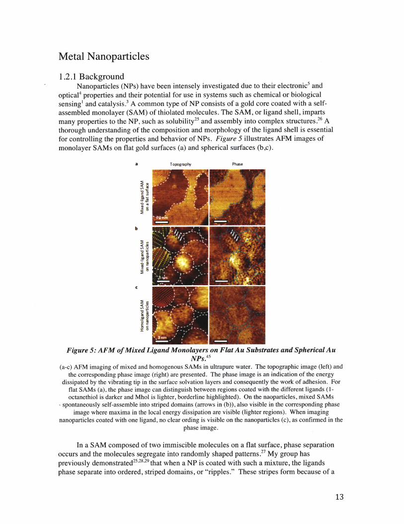
optical4 properties and their potential for use in systems such as chemical or biologicalsensing' and catalysis. 3 A common type of NP consists of a gold core coated with a self-assembled monolayer (SAM) of thiolated molecules. The SAM, or ligand shell, impartsmany properties to the NP, such as solubility25 and assembly into complex structures. 26 Athorough understanding of the composition and morphology of the ligand shell is essentialfor controlling the properties and behavior of NPs. Figure 5 illustrates AFM images ofmonolayer SAMs on flat gold surfaces (a) and spherical surfaces (bc).
a Topography Phase
- gV
IL
kA-
o'-
Zg
Figure 5: AFM of Mixed Ligand Monolayers on Flat Au Substrates and Spherical AuNPs.45
(a-c) AFM imaging of mixed and homogenous SAMs in ultrapure water. The topographic image (left) andthe corresponding phase image (right) are presented. The phase image is an indication of the energy
dissipated by the vibrating tip in the surface solvation layers and consequently the work of adhesion. Forflat SAMs (a), the phase image can distinguish between regions coated with the different ligands (1-octanethiol is darker and Mhol is lighter, borderline highlighted). On the naoparticles, mixed SAMs
- spontaneously self-assemble into striped domains (arrows in (b)), also visible in the corresponding phaseimage where maxima in the local energy dissipation are visible (lighter regions). When imaging
nanoparticles coated with one ligand, no clear ording is visible on the nanoparticles (c), as confirmed in thephase image.
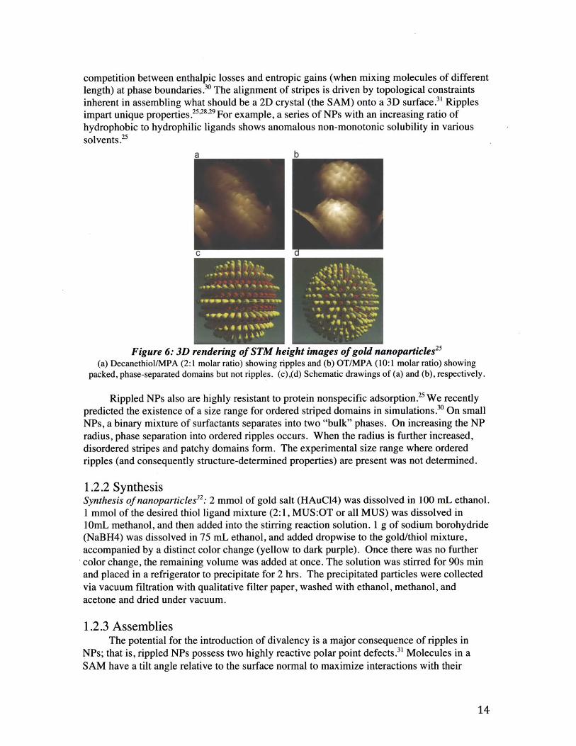
In a SAM composed of two immiscible molecules on a flat surface, phase separationoccurs and the molecules segregate into randomly shaped patterns.2 1 My group haspreviously demonstrated 2 ,28 .2 9 that when a NP is coated with such a mixture, the ligandsphase separate into ordered, striped domains, or "ripples." These stripes form because of a
competition between enthalpic losses and entropic gains (when mixing molecules of differentlength) at phase boundaries.30 The alignment of stripes is driven by topological constraintsinherent in assembling what should be a 2D crystal (the SAM) onto a 3D surface.3' Ripplesimpart unique properties .2s2,29 For example, a series of NPs with an increasing ratio ofhydrophobic to hydrophilic ligands shows anomalous non-monotonic solubility in varioussolvents.2s
Figure 6: 3D rendering of STM height images of gold nanoparticles2s(a) Decanethiol/MPA (2:1 molar ratio) showing ripples and (b) OT/MPA (10:1 molar ratio) showing
packed, phase-separated domains but not ripples. (c),(d) Schematic drawings of (a) and (b), respectively.
Rippled NPs also are highly resistant to protein nonspecific adsorption. 5 We recentlypredicted the existence of a size range for ordered striped domains in simulations.' On smallNPs, a binary mixture of surfactants separates into two "bulk" phases. On increasing the NPradius, phase separation into ordered ripples occurs. When the radius is further increased,disordered stripes and patchy domains form. The experimental size range where orderedripples (and consequently structure-determined properties) are present was not determined.
1.2.2 SynthesisSynthesis of nanoparticles": 2 mmol of gold salt (HAuCl4) was dissolved in 100 mL ethanol.1 mmol of the desired thiol ligand mixture (2:1, MUS:OT or all MUS) was dissolved inlOmL methanol, and then added into the stirring reaction solution. 1 g of sodium borohydride(NaBH4) was dissolved in 75 mL ethanol, and added dropwise to the gold/thiol mixture,accompanied by a distinct color change (yellow to dark purple). Once there was no furthercolor change, the remaining volume was added at once. The solution was stirred for 90s minand placed in a refrigerator to precipitate for 2 hrs. The precipitated particles were collectedvia vacuum filtration with qualitative filter paper, washed with ethanol, methanol, andacetone and dried under vacuum.
1.2.3 AssembliesThe potential for the introduction of divalency is a major consequence of ripples in
NPs; that is, rippled NPs possess two highly reactive polar point defects." Molecules in aSAM have a tilt angle relative to the surface normal to maximize interactions with their
. ........ - -- ------------
neighbors. 27 ,33 For NPs, this tilt angle remains consistent relative to an axis of the NP ratherthan changing on each facet of the crystalline core.' Arranging such a vectorial order(projections of the SAM molecules) onto a topological sphere (a NP core) is only possible iftwo defect points form in diametrically opposed positions on the sphere (Hairy BallTheorem).35 3 6 This implies that two defect sites exist in the ligand shell at which themolecules are not optimally stabilized by intermolecular interactions.
0+ "A HOOC -coo"
IMM MINA~
I S1xw* 9 *6.el's *.*. w 49 w4p 0
~ ~. 9.i;
Figure 7: Chaining of Striped Nanoparticles 3
(a) Two steps of chain formation: pole functionalization of rippled NPs with MUA then interfacialpolymerization. (b) NP size distributions measured from TEM images. Red is that of the starting NPs,
green is that of chained NPs, and blue is that of unchained NPs. Bars represent the actual distribution; linesare Gaussian fits. The graphs are normalized for better visualization; the average NPs size after chaining is2.7nm in this case. Below left is a cartoon of a rippled NP; below right is a representative TEM image of
NP chains, scale bar 25 nm.
Previously, our group proved that these sites, or "poles", are highly reactive and can beselectively functionalized with a place-exchange reaction." Specifically, we placedcarboxylic acid-terminated molecules at the poles to generate divalent NPs (Figure 7);subsequent reaction of these NPs with diamine molecules generated chains of NPs. Notably,this chemical divalency cannot be introduced in homoligand NPs. Previously, we've shownthat divalent NPs (and consequently rippled NPs) exist only in a certain size range; smallerand larger NPs cannot form chains (Figure 8). With AUC, the true existence andquantification of these assemblies can be accomplished, and characterization of their kineticscan be accomplished by systematic study.
...............
m Churned
Size
0Figure 8: Size distributions before and after chaining for three different sets of NPs"7
Chains form only for NPs in a certain size range. Bars represent actual data; lines are Gaussian fits.Each type of line (solid, dashed, or dashed-dotted) represents one complete set of NPs (starting, unchained,and chained distributions). (a-c) Simulation snapshots of phase separation in mixtures of ligands ofunequal length on spheres of increasing diameter.
............ ...........
Chapter 2 AUC ResultsAny adaptation of a technique to a new macromolecular system should be carefully
calibrated. In the case of AUC, many factors contribute to sedimentation, includingconcentration, temperature, polydispersity, diffusion, shape, rotor speed, path length andshape, etc. In order to standardize the AUC of gold nanoparticles, I began with controlexperiments to account for any non-ideality and to find acceptable ranges (or at leastreasonable initial parameters) for many of these variables. After finding typical conditionsfor SV runs, a simple mathematical treatment was derived in order to transform thesedimentation coefficients to a particle size distribution. AUC was then applied tocharacterize a systematic study of NP synthesis parameters that have remained elusive withother techniques, and finally to complex assemblies of nanoparticles.
2.1 Design of ExperimentsFor these controls, the c(s) model was used. The 2D c(s,fr) model is computationallyintensive, and because the following experiments were designed to probe an experimentalparameter and measure s variation, the 2D model was not necessary.
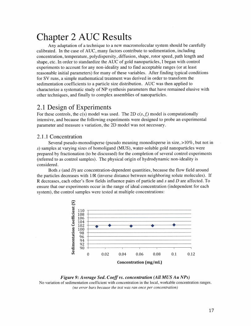
2.1.1 ConcentrationSeveral pseudo-monodisperse (pseudo meaning monodisperse in size, >10%, but not in
s) samples at varying sizes of homoligand (MUS), water-soluble gold nanoparticles wereprepared by fractionation (to be discussed) for the completion of several control experiments(referred to as control samples). The physical origin of hydrodynamic non-ideality isconsidered.
Both s (and D) are concentration-dependent quantities, because the flow field aroundthe particles decreases with 1/R (inverse distance between neighboring solute molecules). IfR decreases, each other's flow fields influence pairs of particle and s and D are affected. Toensure that our experiments occur in the range of ideal concentration (independent for eachsystem), the control samples were tested at multiple concentrations:
*-W
O 110Z 108S106o 104U 1028 100- 98. 96
8 945 92:5 90
.
C 0 0.02 0.04 0.06 0.08 0.1 0.12
Concentration (mg/mL)
Figure 9: Average Sed. Coeff vs. concentration (All MUS Au NPs)No variation of sedimentation coefficient with concentration in the local, workable concentration ranges.
(no error bars because the test was ran once per concentration)
Actually, because our system uses gold nanoparticles which uniquely absorb light atk=520nm, our minimum and maximum concentrations are in the limit of acceptable arbitraryabsorbance units, above and below which the noise in absorbace becomes intolerableanyway. In this range, the average sedimentation coefficient remains statistically unchanged(Fig. 3). Experimentally this means the concentration should be between 1 and 2 AU,measured first with UV/Vis spectroscopy. A consideration of error and statistics explainsthat the concentration should be maximized in this range, to increase the spatial boundaryresolution for subsequent Sedfit analysis. The experiments in this thesis are all performed inthis concentration range.
In addition to experimental consideration of maximum concentration, a mathematicaltreatment approximates an acceptable 'volume fraction.' 38 Hydrodynamic theory predicts thatthe statistics of particle pairs close in vicinity due simply to random motion can lead toreduced drag on the pair (a pseudo-dimer), and increasing the volume fraction dramaticallyenhances this effect. Therefore, the true s is determined empirically as39:
s = s"(1 - 6.55<) (Eq. 2.1)
This equation is valid up to volume fraction < 0.05 and for non-interacting systems.In the range of concentration determined above (e.g. 0.01mgs-0.1mgs), our volume fractionranges from 0.0005-0.0008, thus our error in s is less than >0.01%, much less than thelimiting error due simply to absorbance noise (~1-2%)13 and is thus acceptable.
2.1.2 TemperatureDuring the duration of a single SV experiment, the temperature should fluctuate no
more than 0.5'C .2 The advanced temperature detection system in the XL-I (a radiometer thataccurately senses the actual rotor temperature within 0.05'C advertised precision) records thetemperature at each radial scan. Fluctuations in temperature greater than 0.5'C during asingle experiment leads to a convective instability that is best avoided. Experimentally, whenthe sample is loaded into the AUC and allowed to come to desired temperature, 1 hour shouldbe allowed for sample equilibration and thus convective stability. For most applications andfor every experiment in this thesis, 20'C was used for the absolute temperature. The range ofallowed temperatures in the AUC is from 40C to 220C, but these weren't tested with oursystem.
2.1.3 Polydispersity, diffusion, and speedAs acknowledged in the introduction, the Lamm equation modeling of complex
boundaries from polydisperse samples can be problematic, due to the uncertainty indetangling multiple steps in the concentration profile from noise. Because Lamm equationsolutions can be superpositions of single particle solutions, the shape of the boundary is fittedto approximate multiple particles. Two species with close values of sedimentation coefficientrun at sufficiently fast speed will separate into two steps in a single concentration profile(Fig. 3). Sedimentation mass transport occurs linearly with time, while diffusion goes withthe square root of time, so at the limit of infinite time, sedimentation dominates.Experimentally, this means that high-speed spins can extensively decrease the influence ofdiffusion (particularly useful for quick c(s) modeling to get a general size distribution), andthe elucidation of accurate s values can be ascertained, with the confidence that the boundaryspreading is due to heterogeneity in s, not from diffusion. I have found that the best way toaccomplish this is to find a speed in which the visible resolution of steps (not always possible
for very heterogenous species) can be obtained, for example, in Figure 10:
I -2
0 03"
Distance from rotor center, r (cm)
Figure 10: Experimental boundary profile showing resolvable steps for separate species.At long times (yellow to red) the nanoparticles visibly separate into discrete sedimenting bands. The set offunctions that fit these experimental curves is a solution to the general Lamm equation, yeilding s and D.The red arrows indicate the clear stepped boundary midpoints formed by discrete, sedimenting species.
As a loose experimental rule for metal nanoparticles, 20krpm serves a good startingpoint for an initial run to capture your species. Eventually speeds upwards of 40krpm can beused for smaller species. Monodisperse species, however, can be run at a much slower speedand analysis of the boundary shape (which would be a theoretical step function without thediffusion term in the Lamm equation) can give information on diffusion and a comparison ofdiameter from diffusion and diameter from sedimentation can be achieved. Priorfractionation of polydisperse samples followed by AUC can be used in the same way to gainshape (and thus surface structure) information and is treated in Section 3.3.1.In general high rotor speed (above 30,000 rpm) leads to higher resolution in s and lowerinfluence of D. Using complete data sets from the beginning to the end of sedimentationalso increases resolution (without sufficient sedimentation time, c(s) is ill-defined).
2.1.4 Radial Step SizeWhile scanning across the cell, an adjustable parameter is the rate of scanning by
selecting a scanning step size. The default step size (for a 14 mm cell) is 0.03 mm, howeverthis can be adjusted depending on how many cells are ran concurrently, as the instrumentscans only one cell at one step at a time. For three cells, the first cell is scanned from 0 to 14mm at 0.03 mm steps (-450 points), followed then with the second and third cell, beforecoming back around to the first. At high speeds, significant sedimentation occurs in each cellin between scans, and much information can be missed. In this case, it is advantageous todecrease the radial resolution by increasing step size to 0.1 mm. Generally, samples arethemselves run 'quick-and-dirty' (20 0C, 20 krpm, 0.1 mm) in an effort to elucidate thepreferred step size, and whether or not other samples can be run concurrently withoutreducing the available sedimentation information. This information isn't wasted, because itcan be combined in a global analysis with the eventual high quality information at theoptimal parameters. In the end, each sample has it's own optimization process, and thisshould be perfected to achieve the most accurate size-distribution information.
I
2.2 Particle Size Distribution
2.2.1 c(s) modelConsidering that the NP is made of two concentric spheres, each with constant density
(Pcore and Pigand), a weighted density equation can be derived (full derivation in AppendixA):
p = pg ( p ,core - plig)r,
(Eq. 2.3)
and combining with Eq. 1.9, a functional dependence between NP diameter (d,) andsedimentation coefficient (s), (given pcore, and Pligand ) goes as:
Plotting particle diameter (d,) as a function of s for multiple values of ligand radius andtaking constant the core density and shape (spherical gold core: Pcore=19.3 g/cm 3), liganddensity (P1igadn1.2 g/cm 3) solvent viscosity (11,=0.01002 N sec/m 2), and solvent density ( p
W=0.997 g/cm 3), yields the following curves:
18 i
MUS:OT, All MUS
- MPSA:OT
All MPSA
0 200 400 600 800 1000 1200
Sedimentation Coefficient, s (1A-13 sec)
Figure 11: NP Diameter as a function of Sedimentation Coefficient for Varying LigandSystems.
'0000/. "00
A species of MUS:OT NPs was run at varying speeds and globally analyzed to obtain abest-fit c(s) function:
0.020.018
0.0160.0140.012
0.010.0080.0060.0040.002
0100 200 300 400
Sedimentation Coefficient (S)
0.05-
0-
500 600
61 63 6.4 6.5 6.6 6.7 6.8 6S9 7
Figure 12: c(s) for MUS:OT (2:1) AuNPs.Top: c(s) distribution function; Bottom: visual representation of residual error under a bitmap with
(x,y,contrast(-0.5blik,0.5,e,)=(radius from rotor center, time, local residuals).
To convert to core diameter, Eq. 2.4 can be written as a polynomial (substituting 'x' fortotal diameter, and defining a few constants):
s=ax2 (d+b (xC)3)
a = 1/ 18- r, , b = (p,. - pg) , c =lg , d = (plg - p,) (Eq. 2.5a-c)
s = (ad + ab)x2 - 3abcx + 3abc2 _ abc3
x
This polynomial can be solved for each value of s iteratively using mathematicalanalysis software (such as Matlab) to yield the following distribution:
-A
-A
-
-I-V
0.020.0180.016
3 0.014
o 0.0120.01
0.0080.006
u 0.0040.002
2 3 4 5 6 7 8 9 10 11 12
Core Diameter (nm)
Figure 13: Core diameter for MUS:OT (2:1) AuNPs.
This conversion from s to diameter takes into account assumptions such as theapproximation of all sedimenting species as ideal, non-interacting hard spheres. The ligandlength was taken as the approximate length of the outer ligand, MUS = 1.8nm (calculated inChemDraw @).
The c(s) distribution is highly smoothed, but well determined, and normalized fromtotal loading concentration, so the frequency is quantitative when multiplied by the loadingvalue. A more accurate approach would take into account a variable frictional coefficient,which in reality actually frees the model from any thermodynamic assumption of a D(s)scaling law (Eq. 1.12).
2.2.2 c(s, f/fO) 2D modelThe c(s,f/fO) model outputs a two dimensional value distribution plot following fitting,
including s, RH, D, f/fO, and c(s,f/f0). The s and D are experimentally determined from fittingto the data by a least-squares regression, free of any scaling laws for D(s) or anything else."The D is converted to RH, and f/fO is fitted for each value of s and D and the constant inputpartial specific volume (v). In our case, the partial specific volume is in fact not constant, sorather a value was chosen (<O.1cm 3/g) as to avoid f/fO values close to zero, which compressesthe 2D contour curves. This makes the f/fO value 'fake' for our system, insteadcompensating for a variable v.
The two values s and D can independently be converted to diameter, the s fromiteritively solving Eq. 2.5c and D from:
RTd1, (D) = T (Eq. 2.6)
ND- 3; r,
These values should be in good agreement for spherical particles in which our inputvalues for densities and viscosites are valid. A Matlab script was written to easily convertfrom the 2D distribution to a diameters-diameterD plot (Appendix B).
........... WWWWWO-
-A
-A
-A
The simplest, near-ideal case that could be experimentally measured and modeled withc(s,f/fO) is a population of average-sized, monodisperse, homoligand gold nanoparticles.Dodecanethiol (DDT=1.6nm) gold nanoparticles were synthesized by the Stucky method."Figure 14 shows the particle distribution:
2
sedirnentation coeffcen(S "
0F Adiameter from s (nm)
Figure 14: Particle Size Distribution for DDT homoligand monodisperse NPsThe above image represents the c(sff0) for the DDT monodisperse NPs. The lower image represents the
diameter-diameter plot, each from the sedimentation coefficient and diffusion coeffcient, respectively.(Svedberg and Stokes-Einstein equations).
The DDT NPs exhibit a nearly symmetric diameter-diameter plot. The greaterspreading in diameterD compared to diameters is due to the lower input resolution in Sedfit.Recall from the discussion of error that s is much better defined than the diffusivity, due tothe shape of the boundary curves. The regularization is high in the D direction, to achieve amore parsimonious agreement to the data, which translates to uncertainty in the shape of theprojected ff0 axis c(s,ffO)." In other words, the single peak pictured in Fig. 14 may actuallybe thinner or contain multiple thin peaks, which are unresolvable under the currentexperimental conditions.
.................
2.3 Assemblies
2.3.1 DimersDue to the ability to functionalize the surface of the NPs, assemblies can be formed
through chemical linkage. The following distribution of NPs were synthesized, coated with a2:1 molar mixture of hexadecanethiol and 11-mercaptoundecaneamine:
0 50 100 150s-value (S)
200 250
Runs test Z Istdd" = 1.5vbar = 0.3000
AS 44
Figure 15: c(sflfO) for HDT:MUAM (2:1) AuNPs.
Because the synthesis was tailored in order to produce a small size distribution of NPs,in which the ligands theoretically phase separate into two domains due to the high surfacecurvature. These two-faced 'Janus' particles would only be able to form dimers, trimers, ortetramers by this reaction scheme. The NPs were reacted with activated dicarboxylic acidgroups in order to link the NPs into dimers.
0.025
0.02
0.015
0.01
0.005
A aL IAA A A.A. MMF
'k IIA k A
0.025
4- 0.02
3 -0.015
0101
0 | | 0.00520 40 60 80 100
s-value (S)
Figure 16: c(sffO) for HDT:MUAM (2:1) AuNPs and its DimersThere is a noticeable peak which appears at -80 S, which corresponds to a dimer a 30 S particle.
The existence of the dimer peak is obvious. The sedimentation coefficient of the first peak inthe c(s,*) distribution is 30 S.
Consider the following treatment for the prediction of a dimer and compact trimer andtetramer for a 30 S nanoparticle (the s-value for the peak in Fig. 15. The density of anassembly is unchanged from that of the monomer, and can be calculated using Eq. 2.3. A 29S nanoparticle with ligands HDT:MUAM (2:1) in chloroform corresponds to a total NPdiameter of 5.95 nm (by Eq. 2.4). For the dimer of a 5.95 nm NP, the density is unchanged (p=2.32 g/cm 3) but the axial radius is doubled:
0 IbRaw NP Dimerf - 6mr f -6mygF
for a sphere for an ellipsoid
Figure 17: Frictional Factor of a Raw Nanoparticle vs. the Dimer of that Nanoparticle
For the dimer, the Perrin translational friction factor should be calculated." This fluiddynamics treatment involves the consideration on non-ideality for an oblique spheroid(dimer, trimer, etc.) in terms of its frictional factor and hydrated radius. The Stokes equationin the limit of low Reynolds number (nanoscale) predicts the frictional factor a sphericalobject:
fsphere = 6rls- rm (Eq. 1.7)
with rm the radius of a single NP or monomer. For a non-spherical dimer, the frictionalcoefficient is:
fdi.er = fsphere*' f, (Eq. 2.6)
wheref, is the Perrin frictional factor andfsphere* is the frictional factor for a hard sphere withthe same volume as the ellipsoid of interest:4'
dimer "ans rH s= 6 sq, 1 2)1/3 rM
fP = 2 /
Sp=alb (Eqs. 2.7 a-e)
S2- atanh
p2- 1
p
where VD is the volume of a dimer, which is twice that of it's monomer, VD= 2 Vm. Pluggingthis into the equation adds a factor of 21/3 to the frictional ratio. Finally, the frictional factorfor a non-spherical ellipsoidal 'dimer' is:
This form of the Perrin translational frictional factor simply multiplies a small correctingfactor by the frictional factor for the monomer (given by the Stokes Eq. 1.7). A modifiedSvedberg equation is then:
18* ; - sd =, p,, 1.24 (Eq. 2.9)
Even though the Svedberg equation is derived by assuming a spherical volume, theapproximation of the dimer as an equal volume sphere enables the use of the equation fordimers and assemblies.
Appling this treatment to the 30 S peak in the pre-dimer reaction NP distribution yieldsan approximate value of 80 S, the location of a new peak in the post-dimer NP distribution.
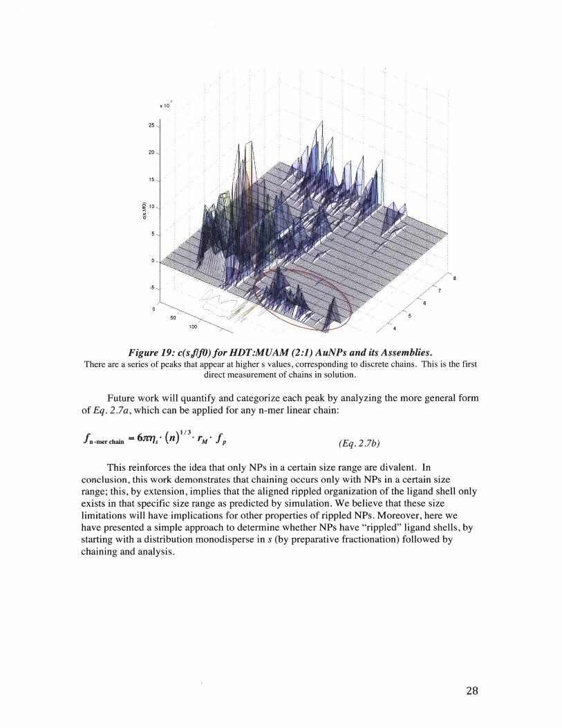
2.3.2 ChainsTo synthesize chains, gold NPs coated with a 2:1 molar mixture of hexadecanethiol and
11-mercaptoundecaneamine typically undergo a two-step reaction.37 The first step is polefunctionalization, a place-exchange reaction at the polar defect sites, in which the NPs are
stirred with a small excess (typically -20-fold) of 11-mercaptoundecanoic acid (MUA), andthen filtered to remove unreacted MUA. The second step is an interfacial polymerization inwhich the NPs in toluene react with a water solution of 1,6-diaminohexane. A precipitateappears at the interface, indicating the formation of insoluble chains. Transmission electronmicroscopy (TEM) is normally used to characterize the precipitate and the supernatant and todetermine the NP size distribution. However, in this work, because the terminal functionalgroup of the outer ligand is an amine, the chaining reaction is simplified to a single combinedstep of a one-phase pole functionalization with the dicarboxylic acid linker molecule. Thefollowing relatively complex c(s,*) distribution of NPs were synthesized, yet unlike the NPsprepared for dimerization, these NPs are larger in size, in the expected size range forordering, or 'striping': 37
0.02
200.01 18
-0.01 -. 01
1500
200 ..... 4
250 30 * 2
350 400 0 f
Figure 18: c(sf/fO) for HDT:MU AM (2:1) A uNPs.
The NPs were then reacted with linker molecules to selectively functionalize the polesof the 'striped' population, in order to form linear assemblies, from dimers to trimers and n-mer chains. The resulting monomer/assemblied solution was examined with AUC andoverlaid on the initial raw data:
25-
20-
15-
5-
0 -
0
50' 5
Figure 19: c(sfJO) for HDT:MUAM (2:1) AuNPs and its Assemblies.There are a series of peaks that appear at higher s values, corresponding to discrete chains. This is the first
direct measurement of chains in solution.
Future work will quantify and categorize each peak by analyzing the more general formof Eq. 2.7a, which can be applied for any n-mer linear chain:
fn-mer chain = 6x,- (n)"- rM fp (Eq. 2.7b)
This reinforces the idea that only NPs in a certain size range are divalent. Inconclusion, this work demonstrates that chaining occurs only with NPs in a certain sizerange; this, by extension, implies that the aligned rippled organization of the ligand shell onlyexists in that specific size range as predicted by simulation. We believe that these sizelimitations will have implications for other properties of rippled NPs. Moreover, here wehave presented a simple approach to determine whether NPs have "rippled" ligand shells, bystarting with a distribution monodisperse in s (by preparative fractionation) followed bychaining and analysis.
Chapter 3 FractionationFractionation of nanoparticles describes the separation by sedimentation constant.
Given the unique surface properties for nanoparticles, specifically as a function of increasingsize or change in shape, the need for selective bulk separation is clear. Fortunately AUCinstrumentation allows the measurement of the s-distribution. The treatment above can beused to determine diameter and shape, and small changes in surface structure can be inferred.This approach enables the testing of nanoparticle function over a range of sizes. The'resolution' of fractionation methods available currently is basically unusable, and nopreparative method exists to fractionate tightly distributed bands of nanoparticles.
3.1 Experimental ProceduresA sucrose gradient was implemented for the bulk preparative fractionation of water-
soluble nanoparticles. The density range of the gradient varies linearly from the tube top tothe bottom, such that the density of the particles is greater than the medium at all points. Thebasic principle is that larger particles sediment faster through the gradient than small ones,just like in a uniform solvent (this is also the fundamental principle of AUC).16
A small aliquot of nanoparticles in solution (M = 5 mg/mL) was carefully layered ontop of a sucrose gradient (20%-50%) in a 13 mL preperative centrifuge tube (for the SW41 TiRotor). The sample was accelerated to 41000 rpm (rotor max speed) and removed after sometime (on the order of one hour).
The following was observed for centrifugation of MUS:OT (2:1) NPs. The existenceof bands can be seen overlayed on a diffuse continuous distribution of nanoparticles. Theposition can be measured and selectively fractionated with a Biocomp@ fractionator, capableof sub millimeter fraction resolution.
Figure 20: Density Gradient Fractionation Band Measurement
3.2 General Gradient Model
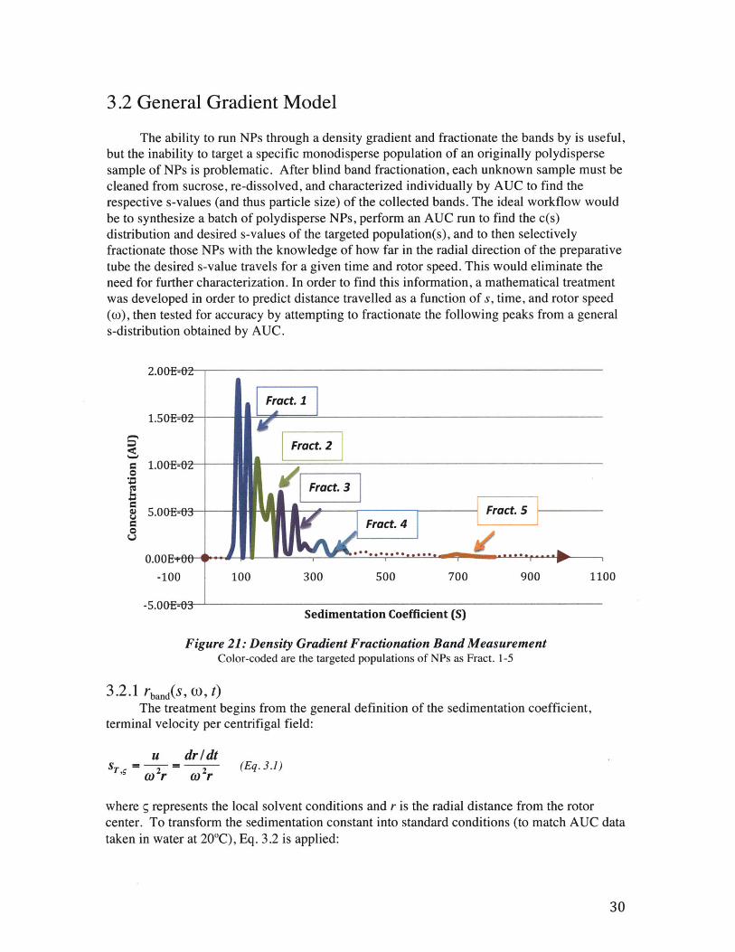
The ability to run NPs through a density gradient and fractionate the bands by is useful,but the inability to target a specific monodisperse population of an originally polydispersesample of NPs is problematic. After blind band fractionation, each unknown sample must becleaned from sucrose, re-dissolved, and characterized individually by AUC to find therespective s-values (and thus particle size) of the collected bands. The ideal workflow wouldbe to synthesize a batch of polydisperse NPs, perform an AUC run to find the c(s)distribution and desired s-values of the targeted population(s), and to then selectivelyfractionate those NPs with the knowledge of how far in the radial direction of the preparativetube the desired s-value travels for a given time and rotor speed. This would eliminate theneed for further characterization. In order to find this information, a mathematical treatmentwas developed in order to predict distance travelled as a function of s, time, and rotor speed(o), then tested for accuracy by attempting to fractionate the following peaks from a generals-distribution obtained by AUC.
2.00E-02
Fract. 11.50&-02-A
Fract. 21.00E&2-
Fract. 3
5.00E03- Fract. 5
0.00E+0H
-100 100 300 500 700 900 1100
-5.00E-03Sedimentation Coefficient (S)
Figure 21: Density Gradient Fractionation Band MeasurementColor-coded are the targeted populations of NPs as Fract. 1-5
3.2.1 rband(s, (0, t)The treatment begins from the general definition of the sedimentation coefficient,
terminal velocity per centrifigal field:
u dr/dtS 2s O r (Eq.3.1)
where g represents the local solvent conditions and r is the radial distance from the rotorcenter. To transform the sedimentation constant into standard conditions (to match AUC datataken in water at 20"C), Eq. 3.2 is applied:
...............
77T ,gp - Pzo,.)s,,= S ,(Pp PTg) (Eq. 3.2)
Combining Eq. 3.1 and Eq. 3.2 leads to:
S2 0,,O 2dt = 1/1,w ''T,'(Pp - P20,,) dr (Eq. 3.3a)(P, - PT,S) r
Eq. 3.3 is general for any centrifugation process in a uniform media, but in a sucrose gradientboth the viscosity (TIT,) and the density (PT,,) are functions of the sucrose concentrations andhence of the distance of the medium from the rotor center, r.
S2 0,O2dt =(11/,, - -dr (Eq. 3.3b)
IpP(r) - p,,(r) I r
with 120,w and P20,w as constants. A major disadvantage of sucrose gradient centrifugation isthe necessity of knowing the partial specific volume (p,-1) in order to determine the true
s2O,w. For this treatment, the particle density is determined recursively by initializing anestimated value for each r (from a calibration experiment), which gives an initial s-value thatis transformed to p, by rearranging Eq. 1.9:
taking the local solvent viscosity, TI, and local solvent density, p,, which are both functionsof radius, r, and d,(s) solved by a Matlab code using Eq. 2.5.
The left hand side of Eq. 3.3 can be integrated over the time of centrifugation, t:
s,,,m 2dt = s2 ,,o 2t (Eq. 3.4)
The right hand side of Eq. 3.3b can be numerically integrated using the trapezoidal rule,which approximates definite integrals:4 3
fo F(r)dr =I F(ri)(ril - ri )+ (1 F(r n ) - F(ri )|(rin - rij (Eq. 3.5)0 0
The expected s-value for each position is solved by calculating equal-spaced arbitrarydistances (ri) from the rotor center (for the SW41 Ti starting at the sucrose density meniscus,71.4 mm) to the last point at which the centrifuge tube is perfect cylindrical (146.1 mm, for89 mm standard tubes). Using standard values of sucrose molarity versus density andviscosity at given temperatures, F(r) can be calculated for each distance, ri.
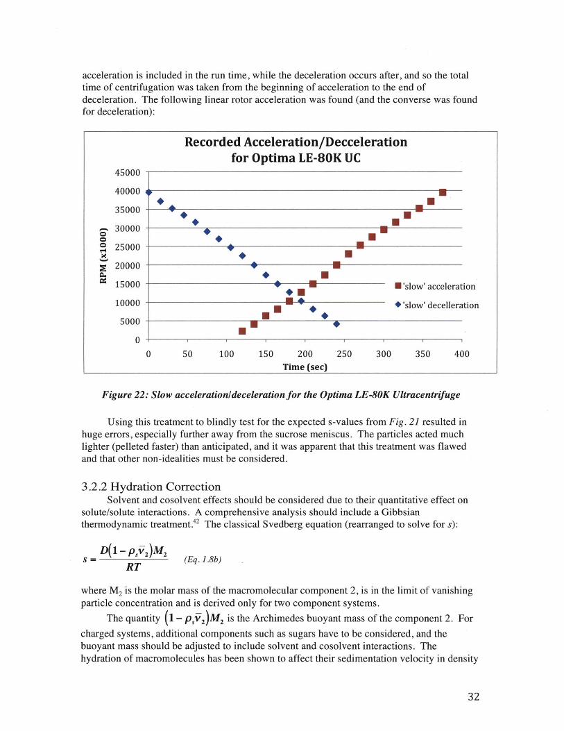
For this treatment the time of centrifugation (t) and rotor speed (o) should be correctedto account for acceleration and deceleration of the rotor, which is unique for each centrifugeand should be found empirically. For the centrifuge used in these experiments, the
acceleration is included in the run time, while the deceleration occurs after, and so the totaltime of centrifugation was taken from the beginning of acceleration to the end ofdeceleration. The following linear rotor acceleration was found (and the converse was foundfor deceleration):
Recorded Acceleration/Deccelerationfor Optima LE-80K UC
45000
40000 1 g
35000 -
30000-
o 25000-
20000 -
15000 - E'slow' acceleration
10000 - *'slow' decelleration
5000-
0
0 50 100 150 200 250 300 350 400Time (sec)
Figure 22: Slow acceleration/deceleration for the Optima LE-80K Ultracentrifuge
Using this treatment to blindly test for the expected s-values from Fig. 21 resulted inhuge errors, especially further away from the sucrose meniscus. The particles acted muchlighter (pelleted faster) than anticipated, and it was apparent that this treatment was flawedand that other non-idealities must be considered.
3.2.2 Hydration CorrectionSolvent and cosolvent effects should be considered due to their quantitative effect on
solute/solute interactions. A comprehensive analysis should include a Gibbsianthermodynamic treatment. The classical Svedberg equation (rearranged to solve for s):
D(1 - p2MS = D -(Eq. 1.8b)
RT
where M 2 is the molar mass of the macromolecular component 2, is in the limit of vanishingparticle concentration and is derived only for two component systems.
The quantity (1 - pfi/ 2 )M 2 is the Archimedes buoyant mass of the component 2. For
charged systems, additional components such as sugars have to be considered, and thebuoyant mass should be adjusted to include solvent and cosolvent interactions. Thehydration of macromolecules has been shown to affect their sedimentation velocity in density
gradients,42 and the hydration can be added to the treatment above.A density gradient of a mixed solvent system can be approximated with 4 components:
1; a light solvent (water), 2- the macromolecule of interest (NPs) 3-a salt, and 4-a heavyneutral component (sucrose). For each position, the sedimentation coefficient at infinitedilution (subscript 0) is given by:4 4
(ap *M- MI
dcSR = T (Eq. 3.6)
RT
where the buoyant molar mass is replaced by the Gibbsian quantity of a density increment atconstant chemical potential, [t, defined as:
-(1-vp) + (1 -vp)+.... (Eq. 3.7)
where ( is a fiting parameter for the particular non-ideality considered. For hydration,B, the hydration constant was used from a tabulated value of 0.3 g/g for sucrose42
The conversion to standard conditions with the hydration correction is:
which can be evaluated by trapezoidal approximation or better, Matlab function analysis.This treatment resulted in a much closer fit to the actual fractionated bands as shown in Fig.23:
Average NP iameter {nm}
' =S.393X - 43 75R =09307930
35
40
45
1 2 3 4Figure 23: Average NP Diameter Down the Tube Following Band Fractionation
Average Particle Diameter (core) as a function of position from the gradient meniscus as measured byTEM. 1-5 represents increasing diameter corresponding to the data points. The dispersity of each diameter
was less than 15%. (Note dark aggregates in TEM images)
The fractionated bands were analyzed again using AUC to determine the accuracy ofselection. Fig. 24 represents the c(s,f/fO) and calculated c(d,,dD):
0.06
0.05A-
0.04-
0.02-
0.01 -
0-
-001
~- - 2105 110 115 120 125 0
s-value (S)
00
6.5
7.5
P 8.5 500 -oa tn* fom D (n"0
Figure 24: Fract. '1': Bimodal Distribution of NP Monomer/Aggregate.
..............
Left: c(s, f/fO) 2D distribution from Sedfit (rmsd = 0.009). Right: calculated c(ds, dD) displaying thediameter-diameter relationship
From the c(s,f/fO) distribution, the experimentally measured s and D coefficients can betransformed separately into particle diameter. The diameter from D can be considered as afunction of size-and-shape, the hydrodynamic size. The diameter from D depends on sizeand shape, but also strongly with density. The sharp peak in Fig. 24 measures -7.3 nm ineach dimension (from both s and D), indicating that population of NPs to be spherical andideal, fulfilling the assumption of core and ligand density (19.3 g/cm 3, 1.2 g/cm 3) and ligandlength (outer ligand MUS: 1.8 nm). Small adjustments and deviations are expected due toassumptions (constant ligand density and length). The spread in diameter of the main peak isfrom 7.21 to 7.42, a dispersity of 3%. The second peak has a hydrodynamic diameter about-7 times that of the diameter from sedimentation coefficient. This peak is likely due toaggregation of a few nanoparticles around sucrose molecule impurities left over from thegradient centrifugation. By the integrated Eq. 3.9, fract. '1' was predicted to be in the s-range of -135 which gives an error of about 0.5 nm from the theoretical value.
ConclusionAUC is powerful tool for investigating nanoparticle size distributions and for detecting
nanoparticle assemblies in solution in their natural hydrated state. A straightforwardtheoretical treatment enables the elucidation of nanoparticles, assemblies, and theirproperties. The program Sedfit serves as a tool to mathematically interpret the raw AUCsedimentation boundary data. For the future, many other types of measurements are possiblewith AUC, such as multi-wavelength measurements that could measure the stoichiometry offluorescently tagged ligands to NPs, in order to study the kinetics of functionalization. Also,more detailed surface structure information or variation of size distribution with change insynthetic parameters can be determined by systematic study. Finally, the sedimentationdistributions provide a map for bulk fractionation of the nanoparticles, which can beseparated for function or study.
Future WorkFor future work, I will attempt to sedimenent nanoparticle samples in a series of mixed
solvents, in order to elucidate the ligand density distribution, measuring ligand density as afunction of size. Also, multi-wavelength experiments are possible, in which thestoichiometry of ligands to nanoparticle can be determined. This could lead to kinetic studiesof surface functionalization and coverage. Also, interacting systems (such as nanoparticlesynthesis) will be monitored and characterized. AUC can also be used to sytematically studynanoparticle synthesis by separately analyzing multiple NP batches that only had onesynthetic parameter changed (e.g. ligand-gold molar ratio: 2:1, 3:1, 4:1). This will enablebetter synthetic control for targeted size distributions.
Appendix A: Derivations
Start with the definition of density:
mp = - (Eq. A.1)
where m is the mass and V is the volume.
m mig +, mScore
VV V
Viig- Pg + Vcore- Pcore
(4;r/3) - (r -3 3,)
pP = Piig (4;rx3) -r Pcore( r1
VU, Vcorepi,- + Pcore
VT T
(4;r/3)- rcore(4;r/3)- r )
3 3 3
". -r ""r(rg 7 - cr + Pcore.(rcore)
hg rT3
pug ri - rcre) + Pcore rcore
* co,,pP = Pig + 3 (Pcore - Pig)
rr
PP =Piig- rr + rcre(pcore - Pi,)
Appendix B: MATLAB code for c(s,f/fO) to c(ds,dD)
%Clears all valuesclear all
%prompt to get file[fileName,pathName] = uigetfile('*.txt','Select AUC Data File'); %prompt to get filerawdata = fileName; % to define the basename of your AUC file
%change command directory to the specified pathNamecd(pathName);
%Load AUC data txt file into the matrix 'data'data = load(fileName);
1. Somers, R. C., et. al. Chem. Soc. Rev. 36,579-591 (2007). BIOLOGY NP2. Verma, A., et. al. Nature Materials, 7, 588 - 595 (2008). BIOLOGY NP3. West, J. L. & Halas, N. J. Annu. Rev. Biomed. Eng. 5, 285-292 (2003).
BIOLOGY NP4. Andres, R. P.; Bein, T.; Dorogi, M.; Feng, S.; Henderson, J. I.; Kubiak, C. P.;
Mahoney, W.; Osifchin, R. G.; Reifenberger, R. Science 1996, 272, 1323-1325.OPTICAL PROPERTY
5. Thomas, K. G.; Kamat, P. V. Acc. Chem. Res. 2003,36, 888-898. ELECTRICPROPERTY
6. Hu, Y. Jour. of Scanning Probe Microscopy. 4,24-35 (2009). STM OF AUNPS7. Centrone, A., Small, 3, 814-817, 2007 STM NPS8. Brown, P.H., Schuck, P., Comput. Phys. Commun. 178, 105-120 (2008) SV
PAPER9. Balbo, A, Brown, P H, Braswell, E H, Schuck, P. Curr Protoc Immunol. 18,
(2007).10. Brown, P H, Balbo, A and Schuck, P. Eur. Biophys. J. 38, 1079-1099 (2009).11. Lebowitz, J., Lewis, M. S., Schuck, P. Protein Sci. 11, 2067-2079 (2002).12. Brown, P H, Schuck, P, Biophys J. 90, 4651-4661 (2006). F/FO PAPER13. Lebowitz, J, Lewis, M S , Schuck, P. Protein Sci. 11, 2067-2079 (2002)14. Balbo, A., Schuck, P., et. al., Proc. Natl. Acad. Sci. USA. 102, 81-86 (2005).15. Machtle, W., Borger, L. Analytical Ultracentrifugation of Polymers and
Nanoparticles. New York: Springer, (2006). Print.16. Schuck, P. Biophys. J. 78, 1606-1619. (2000).17. Schuck, P. Biophys. J. 82, 1096-1111 (2002).18. Schuck, P. In Modem Analytical Ultracentrifugation: Techniques and Methods.
Cambridge, UK: The Royal Society of Chemistry (2005). Print.19. Svedberg, T., Pederson, 0. The Ultracentrifuge. London, UK: Oxford University
Press (1940). Print.20. Schuck, P. 2005. www.analyticalultracentrifugation.com/references.htm. Online.21. Phillips, D. L. Assoc. Comput. Mach. 9, 84-97 (1962).22. Hansen, P.C. Rank-Deficient and Discrete Ill-Posed Problems: Numerical Aspects
of Linear Inversion. Philadelphia: SIAM, (1998). Print.23. Dam, J., Schuck, P. Methods Enzymol. 384, 185-212 (2004).24. Schuck, P., Demeler, B. Biophys. J. 76, 2288-2296 (1999).25. Jackson, A.M., Myerson, J.W., Stellacci, F. Nat. Mater. 3, 330-336 (2004).26. Zhang, Z. L., Horsch, M. A., Lamm, M. H., Glotzer, S. C. Nano Lett. 3, 134 1-
1346 (2003).27. Schreiber, F. Prog. Surf. Sci. 65, 151-256 (2000).28. Jackson, A. M.; Hu, Y.; Silva, P. J.; Stellacci, F. J. Am. Chem. Soc. 128, 11135-
11149 (2006).29. Centrone, A.; Hu, Y.; Jackson, A. M.; Zerbi, G.; Stellacci, F. Small, 3, 814-817
(2007).
30. Singh, C.; Ghorai, P. K.; Horsch, M. A.; Jackson, A. M.; Larson, R. G.; Stellacci,F.; Glotzer, S. C. Phys. ReV. Lett. 99, 226106 (2007).
31. DeVries, G. A.; Brunnbauer, M.; Hu, Y.; Jackson, A. M.; Long, B.; Neltner, B.T.; Uzun, 0.; Wunsch, B. H.; Stellacci, F. Science, 315, 358-361 (2007).
33. Love, J. C.; Estroff, L. A.; Kriebel, J. K.; Nuzzo, R. G.; Whitesides, G. M. Chem.ReV. 105, 1103-1169 (2005).
34. Luedtke, W. D.; Landman, U. J. Phys. Chem. B. 102, 6566-6572 (1998).35. Nelson, D. R. Nano Lett. 2, 1125-1129 (2002).36. Poincare, H. J. Math. Pure Appl. 1, 167 (1885).37. Carney, R., et. al., J. Am. Chem. Soc. 130, 798-799 (2008).38. Evans, W. Fish, J. Keblinski, P. Appl. Phys. Lett. 88, 093116 (2006).39. Planken, K. L., Philipse, A. P. J. Phys. Chem. B. 113, 3932-3940 (2009).40. Zheng, N., Fan, J., Stucky, G. J. Am. Chem. Soc. 128, 6550-6551 (2006).41. Cantor, C.R. Schimmel, P.R. Biophys. Chem. 561-562 (1980).42. Ebel, C., Eisenberg, H., Ghirlando, R. Biophys. Journ. 78, 385-393 (2000).43. Nieuwenhuysen, P. Biopolymers. 18, 277-284 (1979).44. Eisenberg, H. Biophys. Chem. 88, 1-9 (2000).45. Voitchovsky, K. D., Kuna, J., Stellacci, F. Nat. Mat. 8, 837-842 (2009).