1

9 Pulse Characterization

9.3 Frequency Resolved Optical Gating (FROG)

9.4 Spectral Interferometry and SPIDER

9.5 Two-Dimensional Spectral Shearing Interferometry

10 Femtosecond Laser Frequency Combs

Ultrafast Optical Physics II, SoSe 2014, May 9,

Lecture 5, Franz X. Kärtner

Review: IA, IAC

A laser pulse has the time-domain electric field:

E I(t)1/ 2 exp [ j w 0 t – j (t) ] }

Intensity Phase

(t) ~ Re {

Equivalently, vs. frequency:

exp [ -j j ( w – w 0 ) ]

Spectral Phase

(neglecting the

negative-frequency

component)

E ( w ) ~ ~

I(ww0)1/ 2

What information do we need to fully

determine an optical pulse?

Spectrum

Can be measured by an optical spectrum analyzer.

2

Field autocorrelation measurement is equivalent to measuring the spectrum.

Field Autocorrelation

2 2 *( ) ( ) 2Re[ ( ) ( )]E t E t E t E t dt

2( ) ( ) ( )MIV E t E t dt

2 *( ) 2 ( ) 2Re ( ) ( )MIV E t dt E t E t dt

Pulse energy Field autocorrelation

Beam- splitter

Input

pulse

Delay

Slow

detector

Mirror

Mirror

E(t)

E(t–)

VMI( )

)]([Re)]()([Re)()(Re 11 www IFEEFdttEtE

3

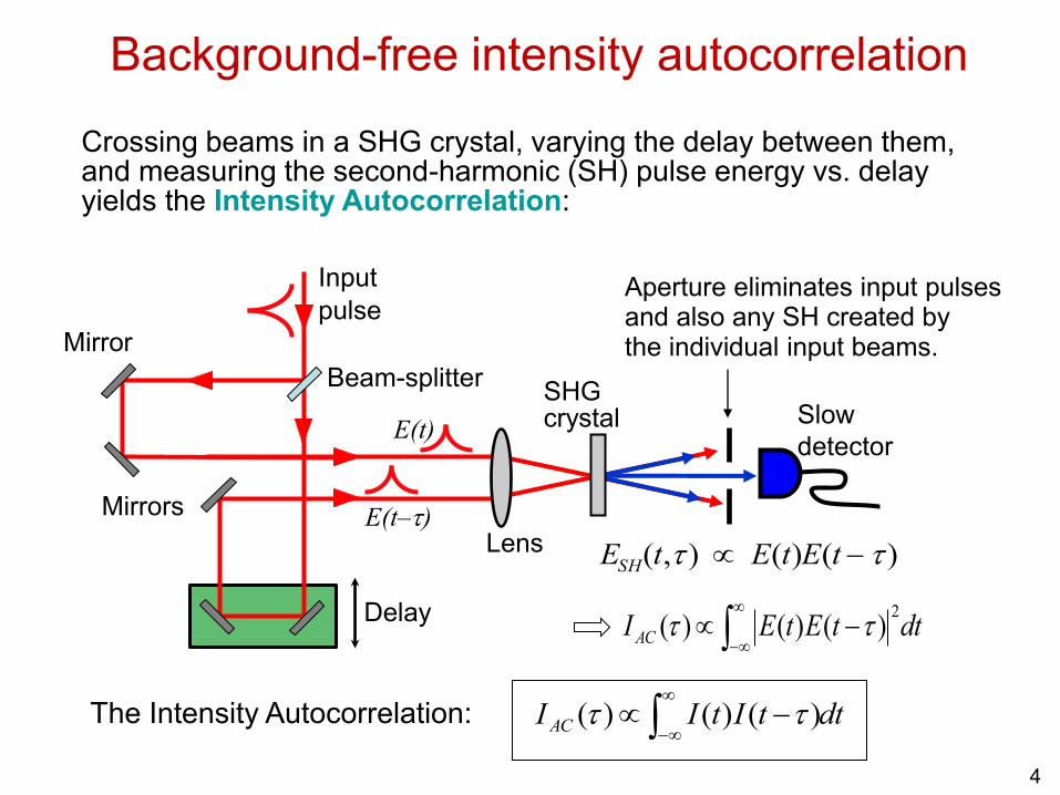
Background-free intensity autocorrelation

dttEtEI AC

2)()()(

Crossing beams in a SHG crystal, varying the delay between them, and measuring the second-harmonic (SH) pulse energy vs. delay yields the Intensity Autocorrelation:

ESH(t, ) E(t)E(t )

The Intensity Autocorrelation:

Delay

Beam-splitter

Input

pulse Aperture eliminates input pulses and also any SH created by the individual input beams.

Slow

detector

Mirror

E(t)

E(t–) Mirrors

SHG crystal

Lens

dttItII AC

)()()(

4

Interferometric autocorrelation (IAC)

),( tE ),(2 tE

What if we use a collinear beam geometry, and allow the autocorrelator

signal light to interfere with the SHG from each individual beam?

Developed by

J-C Diels

Filter Slow

detector SHG

crystal Lens

Beam- splitter

Input

pulse

Delay

Mirror

Mirror

E(t+)

Michelson

Interferometer

Diels and Rudolph,

Ultrashort Laser

Pulse Phenomena,

Academic Press,

1996.

dttEI2

),()(

Photo-detector (or photomultiplier) responds as

5

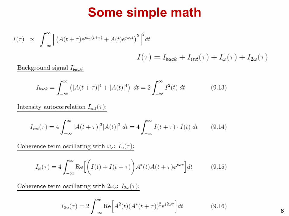
Some simple math

6

Some special moments

7

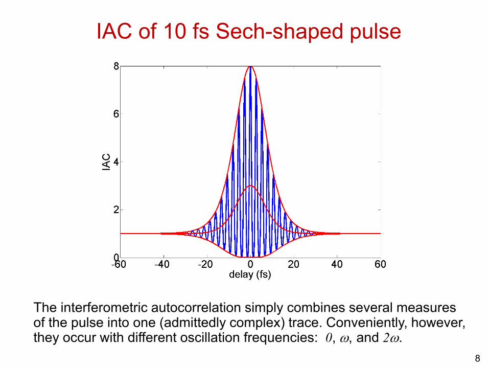
IAC of 10 fs Sech-shaped pulse

The interferometric autocorrelation simply combines several measures of the pulse into one (admittedly complex) trace. Conveniently, however, they occur with different oscillation frequencies: 0, w, and 2w.

8

The spectrogram tells the color and intensity of E(t) at the time, .

We must compute the spectrum of the product: E(t) g(t-)

Esig(t,)

g(t-)

g(t-) gates out a

piece of E(t),

centered at .

Example:

Linearly

chirped

Gaussian

pulse

)(E t

Time (t) 0

Fie

ld a

mp

litu

de

The spectrogram of a pulse

9

If E(t) is the waveform of interest, its spectrogram is:

2

( , ) ( ) ( ) exp( )E E t g t i t dtw w

where g(t-) is a variable-delay gate function and is the delay.

Without g(t-), E(w,) would simply be the spectrum.

The spectrogram is a function of w and .

It is the set of spectra of all temporal slices of E(t).

Mathematical form of a spectrogram

10

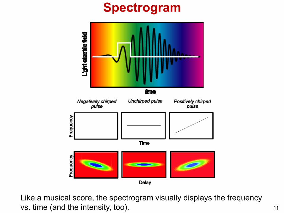
Spectrogram

11

Like a musical score, the spectrogram visually displays the frequency

vs. time (and the intensity, too).

The spectrogram resolves the dilemma! It doesn’t need the shorter

event! It temporally resolves the slow components and spectrally

resolves the fast components.

1) Algorithms exist to retrieve E(t) from its spectrogram. 2) The spectrogram essentially uniquely determines the waveform

intensity, I(t), and phase, (t). There are a few ambiguities, but they’re “trivial.” 3) The gate need not be—and should not be—much shorter than E(t). Suppose we use a delta-function gate pulse:

2

2( ) ( ) exp( ) ( ) exp( )E t t i t dt E i w w

2

( )E = The Intensity. No phase information!

Properties of spectrogram

12

“Polarization Gate” Geometry

Frequency-Resolved Optical Gating (FROG)

Nonlinear medium (glass)

Pulse to be measured

Variable delay,

Camera

Beam splitter

E(t)

E(t-)

Esig(t,) = E(t) |E(t-)|2

FROG involves gating the pulse with a variably delayed replica of

itself in an instantaneous nonlinear-optical medium and then

spectrally resolving the gated pulse vs. delay.

45°

polarization

rotation

Use any ultrafast nonlinearity: Second-harmonic generation, etc.

2

( , ) ( , )exp( )FROG sigI E t i t dtw w

13

The gating is more complex for complex pulses, but it still works.

And it also works for other nonlinear-optical processes.

Polarization gating FROG

14

FROG Traces for Linearly Chirped Pulses

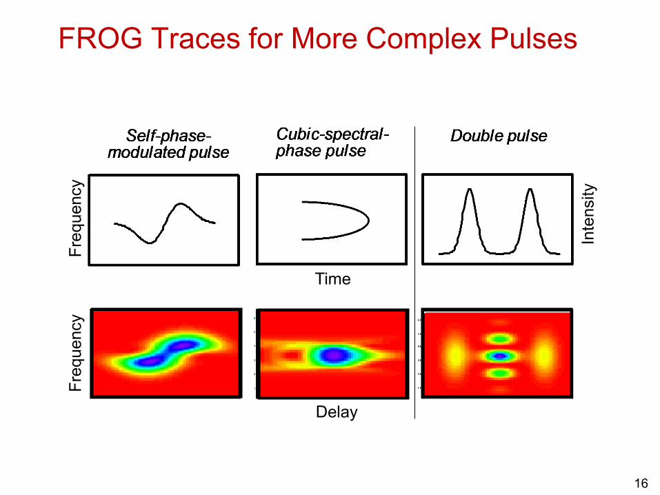
Like a musical score, the FROG trace visually reveals the pulse

frequency vs. time—for simple and complex pulses.

Fre

quency

Fre

quency

Time

Delay

Negatively chirped Unchirped Positively chirped

15

Fre

quency

Fre

quency

Inte

nsity

Time

Delay

FROG Traces for More Complex Pulses F

requency

Delay

16

Ultrashort pulses measured using FROG

FROG

Traces

Retrieved

pulses

Data courtesy of Profs. Bern Kohler and Kent Wilson, UCSD. 17

SHG-FROG

18

19

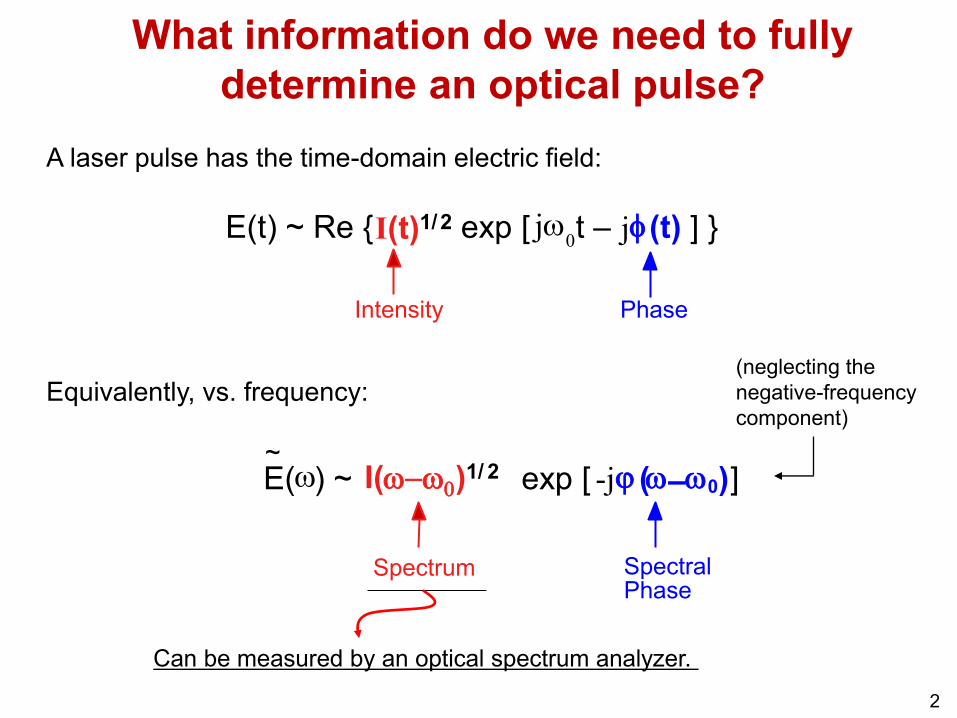
A laser pulse has the time-domain electric field:

E I(t)1/ 2 exp [ j w 0 t – j (t) ] }

Intensity Phase

(t) ~ Re {

Equivalently, vs. frequency:

exp [ -j j ( w – w 0 ) ]

Spectral Phase

(neglecting the

negative-frequency

component)

E ( w ) ~ ~

I(ww0)1/ 2

What information do we need to fully

determine an optical pulse?

Spectrum

Can be measured by an optical spectrum analyzer.

20

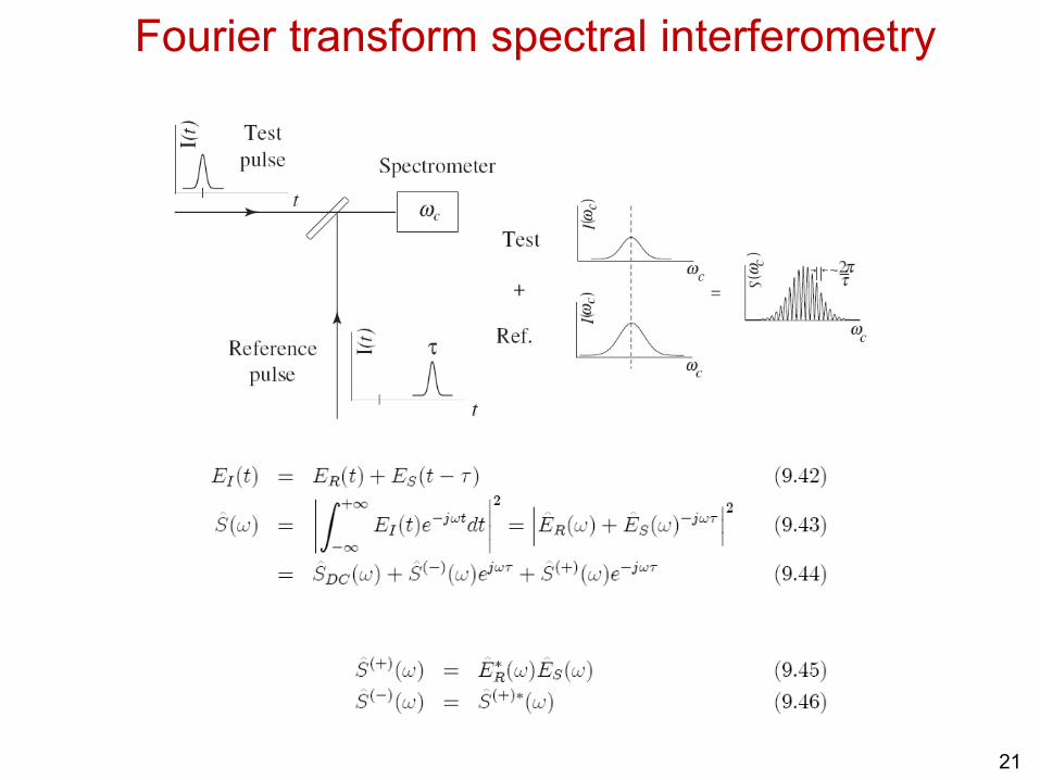
Fourier transform spectral interferometry

21

Inversion algorithm for FTSI

22

SPIDER (Self-Referencing Spectral Interferometry

for Direct Electric-field Reconstruction)

23

Error in delay: D

SPIDER setup

24

Signal detection and phase reconstruction

25

Group delay versus frequency

Measurement Results

26

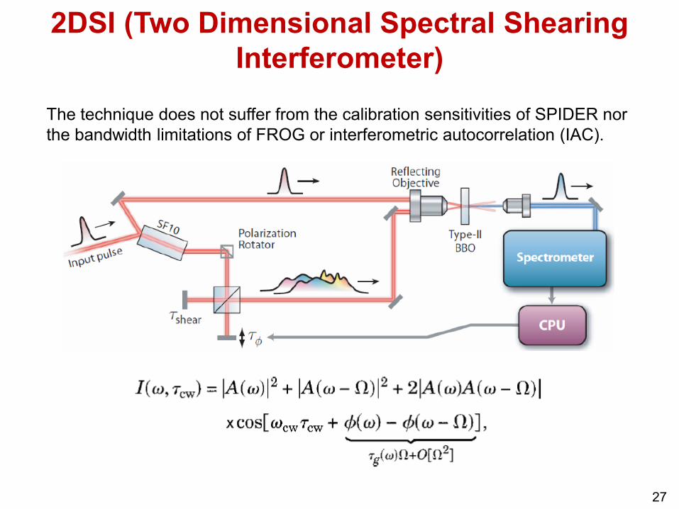
2DSI (Two Dimensional Spectral Shearing

Interferometer)

The technique does not suffer from the calibration sensitivities of SPIDER nor

the bandwidth limitations of FROG or interferometric autocorrelation (IAC).

27

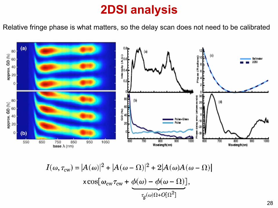
2DSI analysis

Relative fringe phase is what matters, so the delay scan does not need to be calibrated

28

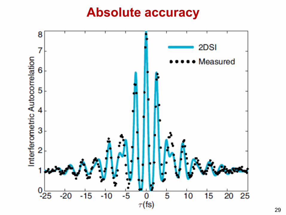
Absolute accuracy

29

30

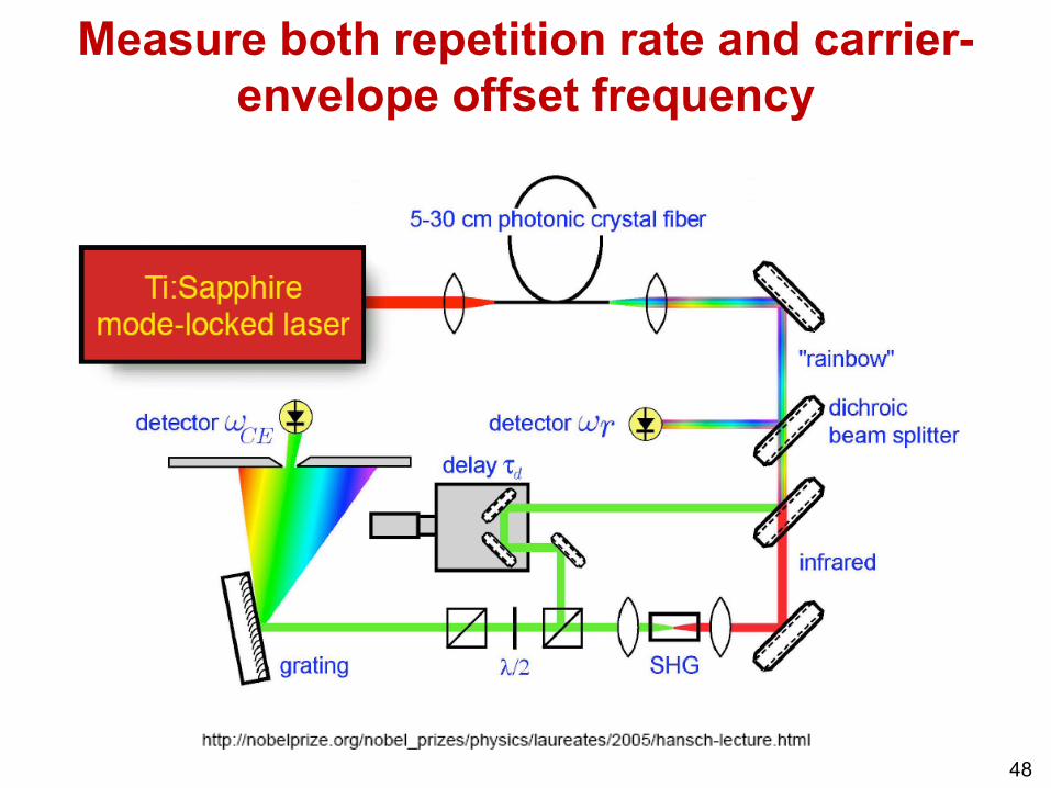
10 Femtosecond Laser Frequency Combs

(Rulers for Light)

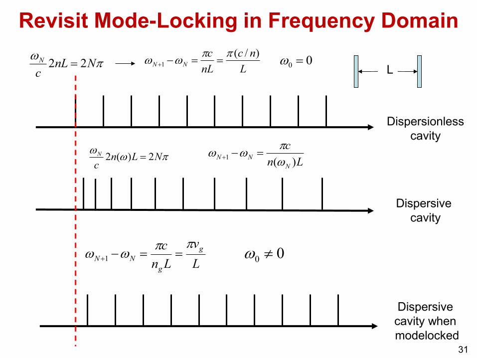
Revisit Mode-Locking in Frequency Domain

w

NnLc

N 22 L

nc

nL

cNN

)/(1

ww 00 w

L

ww

NLnc

N 2)(2 Ln

c

N

NN)(

1w

ww

L

v

Ln

c g

g

NN

ww 1 00 w

Dispersionless

cavity

Dispersive

cavity

Dispersive

cavity when

modelocked 31

Time-Domain Picture

t

t

t

32

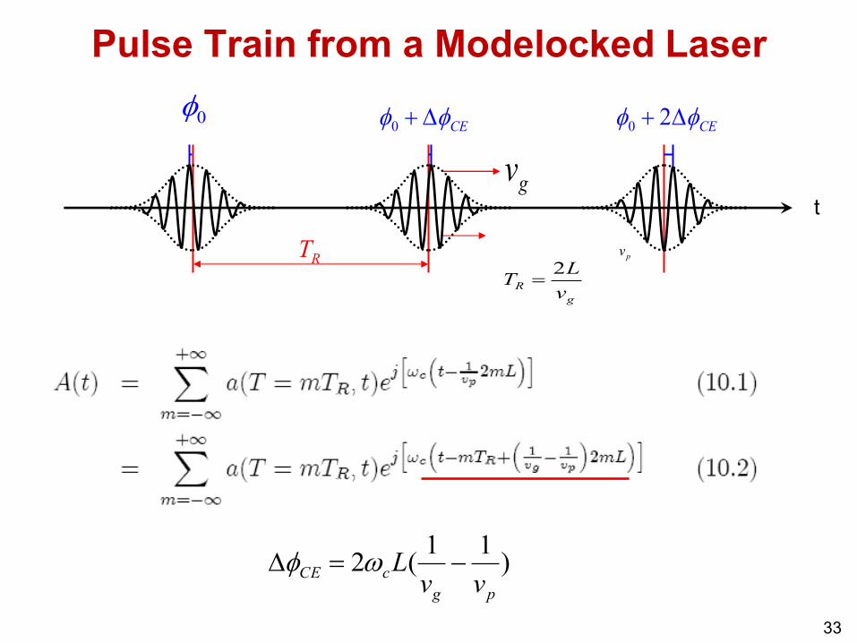
Pulse Train from a Modelocked Laser

0

pv

)11

(2pg

cCEvv

L D w

CE D0 CE D 20

gvt

RT

g

Rv

LT

2

33

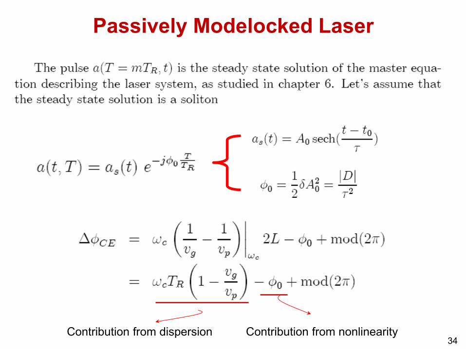
Passively Modelocked Laser

Contribution from dispersion Contribution from nonlinearity 34

Optical Spectrum

35

f

Spectral Envelope

Frequency Comb

f

Carrier Frequency cf

f

0

0

36

Comb has two degrees of freedom

f

D

2mod CE

RCE ff

R

RT

f1

CERm fmff

1) How to measure fCE?

2) How to control fCE or what determines fCE?

3) Does pump power only relate to fCE?

It is straightforward to measure (using RF spectrum analyzer) and

control (i.e. tuning cavity length) fR.

37

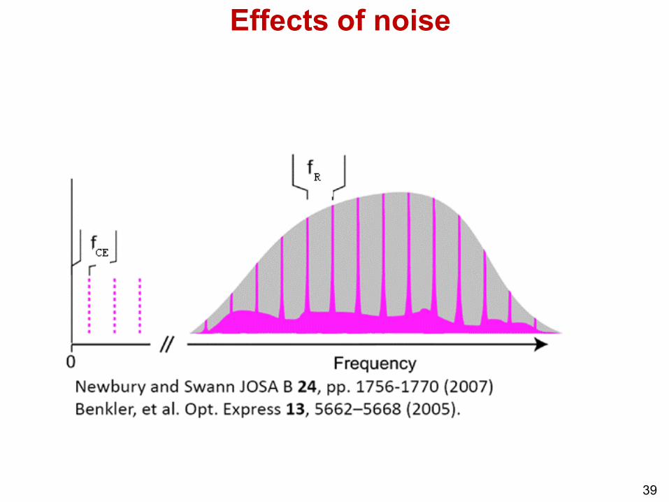
Noiseless frequency comb

CERm fmff

38

Effects of noise

39

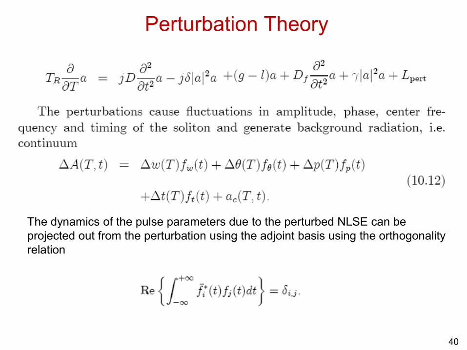
Perturbation Theory

The dynamics of the pulse parameters due to the perturbed NLSE can be

projected out from the perturbation using the adjoint basis using the orthogonality

relation

40

Perturbation theory

Physics behind:

(10.15) a change of soliton energy causes a cumulative change of phase since

the contribution from the Kerr effect has changed.

(10.17) a change of carrier frequency causes a cumulative change of

displacement due to a change in group velocity.

(10.14) & (10.16) due to gain saturation, gain filtering, and saturable absorber

action, the pulse energy and center frequency fluctuations are damped with

decay constants

41

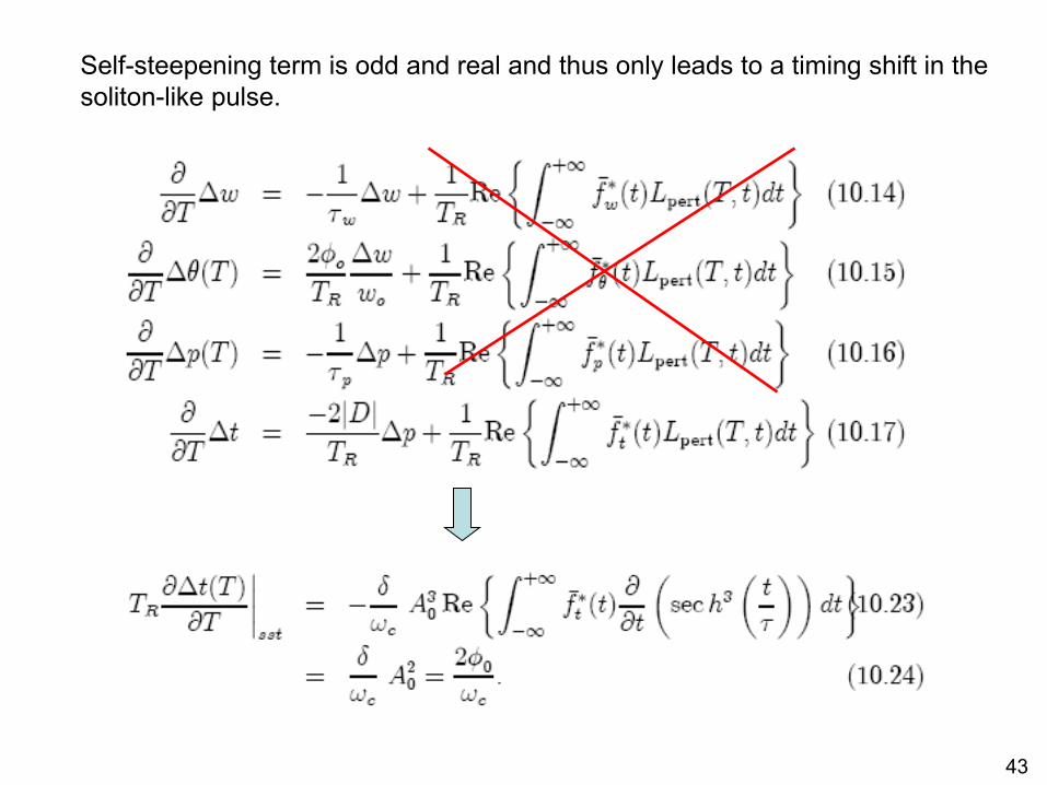
Effect of self-steepening

Even without GVD, significant pulse-

shape distortion can occur if the pulse is

extremely short.

Self-steepening results from the

intensity dependence of the group

velocity, which leads to an asymmetry

in the SPM-broadened spectra of

ultrashort pulses.

42

Self-steepening term is odd and real and thus only leads to a timing shift in the

soliton-like pulse.

43

44

Measure carrier-envelope offset

frequency using 1f-2f Interferometer

ceof

f

power

beat

frequency

ceoR fmF ceoR fmF 2

ceoR fmF 22 45

http://nobelprize.org/nobel_prizes/physics/laureates/2005/hall-lecture.html 46

Phillip Russel, Univ. of Bath, now Max-Planck

Institute for the Science of Light, Erlangen

http://nobelprize.org/nobel_prizes/physics/laureates/2005/hall-lecture.html 47

Measure both repetition rate and carrier-

envelope offset frequency

48

49

50

Bandwidth of Few-Cycle Optical Pulses

Wavelength, µm

Gain

, a.u

.

Ti:sapphire Gain

0.6 0.8 1.0 1.2 1.4

1 Cycle = 2.7 fs @ 800 nm

10 fs ~ 4 cycles (Standard Optics)

2 Cycles = 5.4 fs Chirped Mirrors

One Octave Double-Chirped Mirror

Pairs

First demonstration of octave spanning Ti:Sapphire Laser:

U. Morgner, et al., PRL 86, 5462-5465, 2001.

50

Octave Spanning Oscillator

51

Frequency Metrology

f

power Frequency

to measure Frequency

standard

52

53

What is a Clock?

an oscillator a clockwork

Pendulum - Christiaan Huygens 1656

Chronometer - John Harrison (H4) 1761 (10-6 ~ 1 sec/ 9 days )

Quartz - W. Marrison, Bell Labs, 1928 (10-8 ~ 1 sec/3yrs )

Cesium atom - 1955 (10-10 ~ 1sec/300yrs)

Hg ion – 5x10-18 ~ 10sec since big bang

Atomic fountain - NIST-F1 (1.7x10-15 ~ 1sec/20Myrs)

and

54

fR = 1/TR : pulse repetition rate

fR

f0 = m fR Optical Ref.

Optical Clock

TR

CE 0

Laser CE-phase stabilized Femtosecond Pulse Train

CE 0 CE 0 CE 0 CE 0 CE 0

(n/m) f0

Each microwave cycle = M Optical Cycles

Low noise optical pulse train or microwaves

70MHz

Pump Laser AOM

f/32

LF

HeNe#2

Laser

CH4/HeNe#1

Laser

PBS l/2 570nm

DCMs

PP

LN

LBO

3.39um

HeNe discharge tube

Ti:Sa

LF

LF

~

M. A. Gubin, Lebedev Institute

CH4-HeNe Based Frequency Comb and Clock

A. Benedick, et al. Opt. Lett. 34, pp. 2168-2170, (2009)

1 GHz

55

Optical Arbitrary Waveform Generation

• Require high repetition rate sources to ease (DE)MUX

fabrication requirements

56

Doppler-shift spectroscopy

Th-Ar lamp

or I2 cell

NOT TO SCALE

Astro-comb

spectrograph

C-H. Li, et al., Nature 452, 610-612 (2008).

Astro-comb => remove comb lines with

a stabilized Fabry-Perot cavity to

achieve line-spacing of 40 GHz

58

Th-Ar lamp versus Astro-Comb (Whipple Obseratory, Arizona)

Echelle dispersion

Diffr

actio

n o

rde

rs

Blue

Red

CCD array

ThAr

comb

59