SUMMARY FOR POLICYMAKERS SPECIAL REPORT ON EMISSION SCENARIOS A Special Report of Working Group III of the Intergovernmental Panel on Climate Change Based on a draft prepared by: Nebojs ˘a Nakic ´enovic ´, Ogunlade Davidson, Gerald Davis, Arnulf Grübler, Tom Kram, Emilio Lebre La Rovere, Bert Metz, Tsuneyuki Morita, William Pepper, Hugh Pitcher, Alexei Sankovski, Priyadarshi Shukla, Robert Swart, Robert Watson, Zhou Dadi
Transcript
SUMMARY FOR POLICYMAKERS
SPECIAL REPORT ON EMISSION SCENARIOS
A Special Report of Working Group IIIof the Intergovernmental Panel on Climate Change
Based on a draft prepared by:
Nebojsa Nakicenovic, Ogunlade Davidson, Gerald Davis, Arnulf Grübler, Tom Kram, Emilio Lebre La Rovere, Bert
Metz, Tsuneyuki Morita, William Pepper, Hugh Pitcher, Alexei Sankovski, Priyadarshi Shukla, Robert Swart, Robert
Watson, Zhou Dadi
Why new Intergovernmental Panel on Climate Change scenarios? 3
What are scenarios and what is their purpose? 3
What are the main characteristics of the new scenarios? 3
What are the main driving forces of the GHG emissions in the scenarios? 5
What is the range of GHG emissions in the SRES scenarios and how do they relate to driving forces? 9
How can the SRES scenarios be used? 11
What future work on emissions scenarios would be useful? 11
CONTENTS
Why new Intergovernmental Panel on Climate Changescenarios?
The Intergovernmental Panel on Climate Change (IPCC)developed long-term emission scenarios in 1990 and 1992.These scenarios have been widely used in the analysis ofpossible climate change, its impacts, and options to mitigateclimate change. In 1995, the IPCC 1992 scenarios wereevaluated. The evaluation recommended that significantchanges (since 1992) in the understanding of driving forces ofemissions and methodologies should be addressed. Thesechanges in understanding relate to, e.g., the carbon intensity ofenergy supply, the income gap between developed anddeveloping countries, and to sulfur emissions. This led to adecision by the IPCC Plenary in 1996 to develop a new set ofscenarios. The new set of scenarios is presented in this report.
What are scenarios and what is their purpose?
Future greenhouse gas (GHG) emissions are the product ofvery complex dynamic systems, determined by driving forcessuch as demographic development, socio-economicdevelopment, and technological change. Their future evolutionis highly uncertain. Scenarios are alternative images of how thefuture might unfold and are an appropriate tool with which toanalyze how driving forces may influence future emissionoutcomes and to assess the associated uncertainties. They assistin climate change analysis, including climate modeling and theassessment of impacts, adaptation, and mitigation. Thepossibility that any single emissions path will occur asdescribed in scenarios is highly uncertain.
What are the main characteristics of the new scenarios?
A set of scenarios was developed to represent the range ofdriving forces and emissions in the scenario literature so as toreflect current understanding and knowledge about underlyinguncertainties. They exclude only outlying “surprise” or“disaster” scenarios in the literature. Any scenario necessarilyincludes subjective elements and is open to variousinterpretations. Preferences for the scenarios presented herevary among users. No judgment is offered in this report as tothe preference for any of the scenarios and they are notassigned probabilities of occurrence, neither must they beinterpreted as policy recommendations.
The scenarios are based on an extensive assessment of drivingforces and emissions in the scenario literature, alternativemodeling approaches, and an “open process”1 that solicited
wide participation and feedback. These are all-importantelements of the Terms of Reference (see Appendix I).
Four different narrative storylines were developed to describeconsistently the relationships between emission driving forcesand their evolution and add context for the scenarioquantification. Each storyline represents differentdemographic, social, economic, technological, andenvironmental developments, which may be viewed positivelyby some people and negatively by others.
The scenarios cover a wide range of the main demographic,economic, and technological driving forces of GHG and sulfuremissions2 and are representative of the literature. Eachscenario represents a specific quantitative interpretation of oneof four storylines. All the scenarios based on the same storylineconstitute a scenario “family”.
As required by the Terms of Reference, the scenarios in thisreport do not include additional climate initiatives, whichmeans that no scenarios are included that explicitly assumeimplementation of the United Nations Framework Conventionfor Climate Change (UNFCCC) or the emissions targets of theKyoto Protocol. However, GHG emissions are directly affectedby non-climate change policies designed for a wide range ofother purposes. Furthermore government policies can, tovarying degrees, influence the GHG emission drivers such asdemographic change, social and economic development,technological change, resource use, and pollutionmanagement. This influence is broadly reflected in thestorylines and resultant scenarios.
For each storyline several different scenarios were developedusing different modeling approaches to examine the range ofoutcomes arising from a range of models that use similarassumptions about driving forces. Six models were used whichare representative of integrated assessment frameworks in theliterature. One advantage of a multi-model approach is that theresultant 40 SRES scenarios together encompass the currentrange of uncertainties of future GHG emissions arising fromdifferent characteristics of these models, in addition to thecurrent knowledge of and uncertainties that arise from scenariodriving forces such as demographic, social and economic, andbroad technological developments that drive the models, asdescribed in the storylines. Thirteen of these 40 scenariosexplore variations in energy technology assumptions.
3Summary for Policymakers
1 The open process defined in the Special Report on EmissionsScenarios (SRES) Terms of Reference calls for the use of multiplemodels, seeking inputs from a wide community as well as makingscenario results widely available for comments and review. Theseobjectives were fulfilled by the SRES multi-model approach and theopen SRES website.
2 Included are anthropogenic emissions of carbon dioxide (CO2),methane (CH4), nitrous oxide (N2O), hydrofluorocarbons (HFCs),perfluorocarbons (PFCs), sulfur hexafluoride (SF6), hydrochloro-fluorocarbons (HCFCs), chlorofluorocarbons (CFCs), the aerosolprecursor and the chemically active gases sulfur dioxide (SO2),carbon monoxide (CO), nitrogen oxides (NOx), and non-methanevolatile organic compounds (NMVOCs). Emissions are providedaggregated into four world regions and global totals. In the newscenarios no feedback effect of future climate change on emissionsfrom biosphere and energy has been assumed.
Summary for Policymakers4
Box SPM-1: The Main Characteristics of the Four SRES Storylines and Scenario Families.
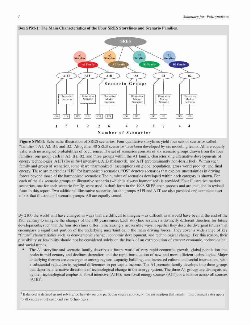
By 2100 the world will have changed in ways that are difficult to imagine – as difficult as it would have been at the end of the19th century to imagine the changes of the 100 years since. Each storyline assumes a distinctly different direction for futuredevelopments, such that the four storylines differ in increasingly irreversible ways. Together they describe divergent futures thatencompass a significant portion of the underlying uncertainties in the main driving forces. They cover a wide range of key“future” characteristics such as demographic change, economic development, and technological change. For this reason, theirplausibility or feasibility should not be considered solely on the basis of an extrapolation of current economic, technological,and social trends.
• The A1 storyline and scenario family describes a future world of very rapid economic growth, global population thatpeaks in mid-century and declines thereafter, and the rapid introduction of new and more efficient technologies. Majorunderlying themes are convergence among regions, capacity building, and increased cultural and social interactions, witha substantial reduction in regional differences in per capita income. The A1 scenario family develops into three groupsthat describe alternative directions of technological change in the energy system. The three A1 groups are distinguishedby their technological emphasis: fossil intensive (A1FI), non-fossil energy sources (A1T), or a balance across all sources(A1B)3.
B2 FamilyB1 FamilyA2 Family
SRES
HS HSOS OS
Illustrative
Marker
Scenario
N u m b e r o f S c e n a r i o s
OS HSOS HS
B2Storyline
B2B1
B1Storyline
A2Storyline
A2
A1Storyline
Illustrative
Scenario
OS HS
Illustrative
Scenario
Illustrative
Marker
Scenario
A1BA1TA1FI
Illustrative
Marker
Scenario
Illustrative
Marker
Scenario
1 5 1 2 2 6 4 2 2 7 4 4
S c e n a r i o G r o u p s
A1 Family
HSOS
Figure SPM-1: Schematic illustration of SRES scenarios. Four qualitative storylines yield four sets of scenarios called“families”: A1, A2, B1, and B2. Altogether 40 SRES scenarios have been developed by six modeling teams. All are equallyvalid with no assigned probabilities of occurrence. The set of scenarios consists of six scenario groups drawn from the fourfamilies: one group each in A2, B1, B2, and three groups within the A1 family, characterizing alternative developments ofenergy technologies: A1FI (fossil fuel intensive), A1B (balanced), and A1T (predominantly non-fossil fuel). Within eachfamily and group of scenarios, some share “harmonized” assumptions on global population, gross world product, and finalenergy. These are marked as “HS” for harmonized scenarios. “OS” denotes scenarios that explore uncertainties in drivingforces beyond those of the harmonized scenarios. The number of scenarios developed within each category is shown. Foreach of the six scenario groups an illustrative scenario (which is always harmonized) is provided. Four illustrative markerscenarios, one for each scenario family, were used in draft form in the 1998 SRES open process and are included in revisedform in this report. Two additional illustrative scenarios for the groups A1FI and A1T are also provided and complete a setof six that illustrate all scenario groups. All are equally sound.
3 Balanced is defined as not relying too heavily on one particular energy source, on the assumption that similar improvement rates applyto all energy supply and end use technologies.
Within each scenario family two main types of scenarios weredeveloped – those with harmonized assumptions about globalpopulation, economic growth, and final energy use and thosewith alternative quantification of the storyline. Together, 26scenarios were harmonized by adopting common assumptionson global population and gross domestic product (GDP)development. Thus, the harmonized scenarios in each familyare not independent of each other. The remaining 14 scenariosadopted alternative interpretations of the four scenariostorylines to explore additional scenario uncertainties beyonddifferences in methodologic approaches. They are also relatedto each other within each family, even though they do not sharecommon assumptions about some of the driving forces.
There are six scenario groups that should be consideredequally sound that span a wide range of uncertainty, asrequired by the Terms of Reference. These encompass fourcombinations of demographic change, social and economicdevelopment, and broad technological developments,corresponding to the four families (A1, A2, B1, B2), each withan illustrative “marker” scenario. Two of the scenario groups ofthe A1 family (A1FI, A1T) explicitly explore alternativeenergy technology developments, holding the other drivingforces constant, each with an illustrative scenario. Rapidgrowth leads to high capital turnover rates, which means thatearly small differences among scenarios can lead to a largedivergence by 2100. Therefore the A1 family, which has thehighest rates of technological change and economicdevelopment, was selected to show this effect.
In accordance with a decision of the IPCC Bureau in 1998 torelease draft scenarios to climate modelers for their input inthe Third Assessment Report, and subsequently to solicitcomments during the open process, one marker scenario waschosen from each of four of the scenario groups based on thestorylines. The choice of the markers was based on which ofthe initial quantifications best reflected the storyline, andfeatures of specific models. Marker scenarios are no more orless likely than any other scenarios, but are considered by theSRES writing team as illustrative of a particular storyline.These scenarios have received the closest scrutiny of the entirewriting team and via the SRES open process. Scenarios have
also been selected to illustrate the other two scenario groups.Hence, this report has an illustrative scenario for each of the sixscenario groups.
What are the main driving forces of the GHG emissions inthe scenarios?
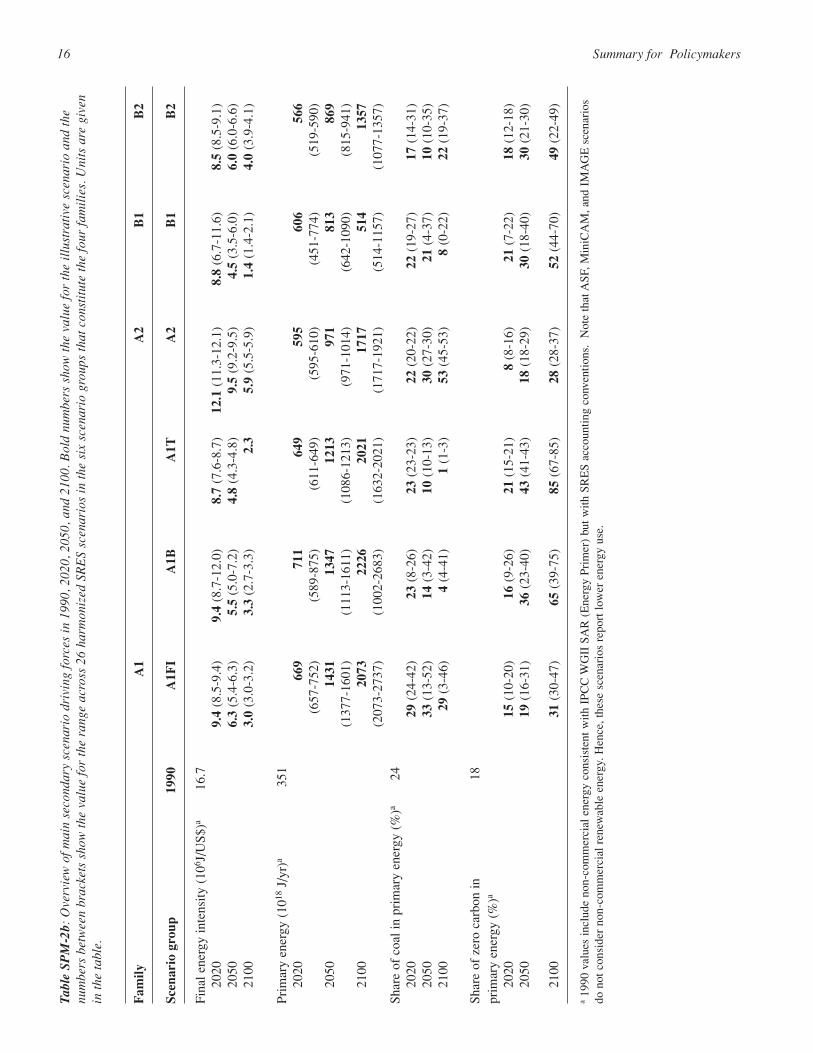
This Report reinforces our understanding that the maindriving forces of future greenhouse gas trajectories willcontinue to be demographic change, social and economicdevelopment, and the rate and direction of technologicalchange. This finding is consistent with the IPCC 1990, 1992and 1995 scenario reports. Table SPM-1 (see later) summarizesthe demographic, social, and economic driving forces acrossthe scenarios in 2020, 2050, and 21004. The intermediateenergy result (shown in table SPM 2, see later) and land useresults5 reflect the influences of driving forces.
Recent global population projections are generally lower thanthose in the IS92 scenarios. Three different populationtrajectories that correspond to socio-economic developments inthe storylines were chosen from recently published projections.The A1 and B1 scenario families are based on the lowInternational Institute for Applied Systems Analysis (IIASA)1996 projection. They share the lowest trajectory, increasing to8.7 billion by 2050 and declining toward 7 billion by 2100,which combines low fertility with low mortality. The B2scenario family is based on the long-term UN Medium 1998population projection of 10.4 billion by 2100. The A2 scenariofamily is based on a high population growth scenario of 15billion by 2100 that assumes a significant decline in fertility formost regions and stabilization at above replacement levels. Itfalls below the long-term 1998 UN High projection of 18billion.
5Summary for Policymakers
• The A2 storyline and scenario family describes a very heterogeneous world. The underlying theme is self-reliance andpreservation of local identities. Fertility patterns across regions converge very slowly, which results in continuouslyincreasing global population. Economic development is primarily regionally oriented and per capita economic growthand technological change are more fragmented and slower than in other storylines.
• The B1 storyline and scenario family describes a convergent world with the same global population that peaks in mid-century and declines thereafter, as in the A1 storyline, but with rapid changes in economic structures toward a serviceand information economy, with reductions in material intensity, and the introduction of clean and resource-efficienttechnologies. The emphasis is on global solutions to economic, social, and environmental sustainability, includingimproved equity, but without additional climate initiatives.
• The B2 storyline and scenario family describes a world in which the emphasis is on local solutions to economic, social,and environmental sustainability. It is a world with continuously increasing global population at a rate lower than A2,intermediate levels of economic development, and less rapid and more diverse technological change than in the B1 andA1 storylines. While the scenario is also oriented toward environmental protection and social equity, it focuses on localand regional levels.
4 Technological change is not quantified in table SPM-1.
5 Because of the impossibility of including the complex way land useis changing between the various land use types, this information is notin the table.
Summary for Policymakers6
0
2
4
6
8
10
1900 1950 2000 2050 2100
GlobalCarbonDioxideEmissions
SRESScenariosandDatabase
Range
(index,1990=1)
IS92range
A1B
A2
B1
1990 range
Maximum in
Database
Minimum in Database
Total database range
Non-intervention
Non-classified
Intervention
B2
A1F1
A1T
-3.5
-2.5
-1.5
-0.5
0.5
1.5
2.5
3.5
1900 1950 2000 2050 2100
1990 range (SAR)
Literature range
maximum
Literature range
minimum
Total database range
A2
B1
A1B
B2
GlobalCarbonDioxideEmissions
Land-use
Change
(index,1990=1)
2025
IS92 range
A1FI
A1T
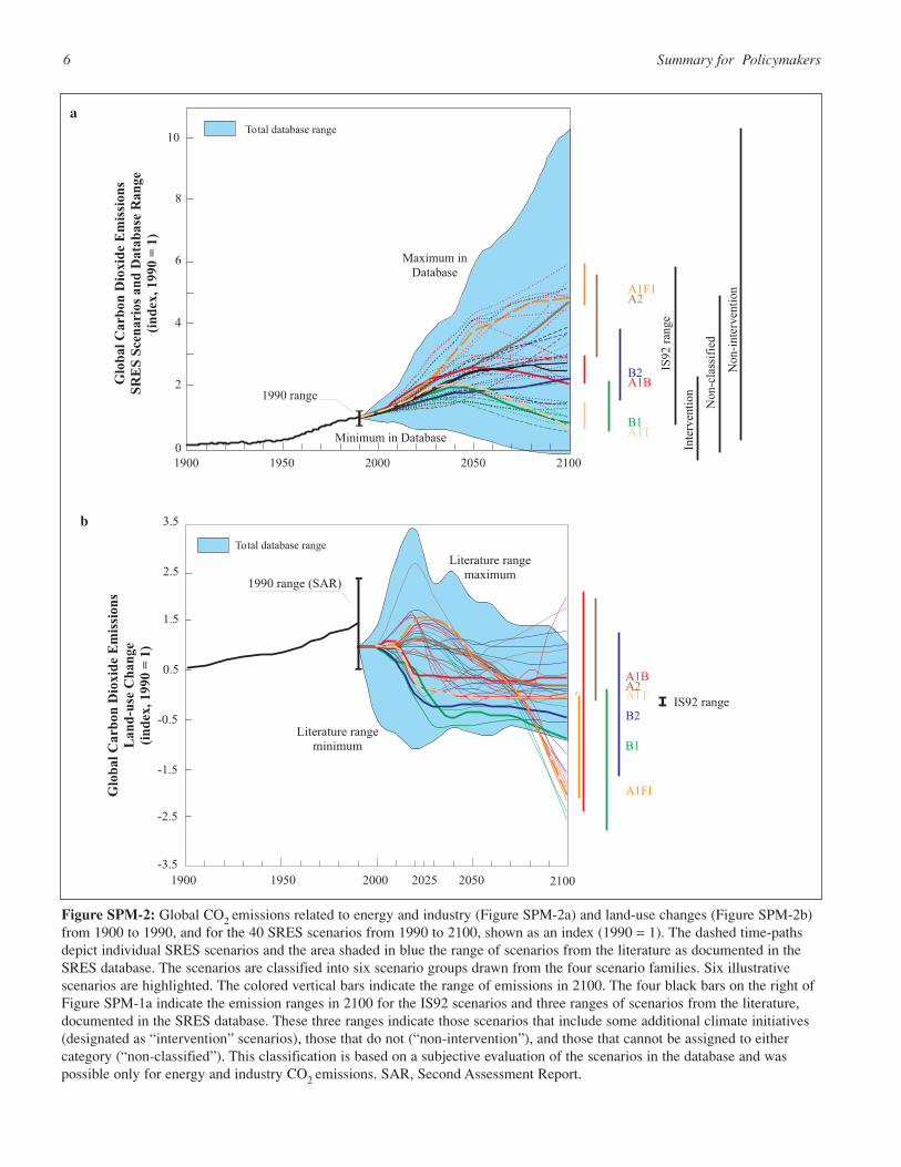
Figure SPM-2: Global CO2 emissions related to energy and industry (Figure SPM-2a) and land-use changes (Figure SPM-2b)from 1900 to 1990, and for the 40 SRES scenarios from 1990 to 2100, shown as an index (1990 = 1). The dashed time-pathsdepict individual SRES scenarios and the area shaded in blue the range of scenarios from the literature as documented in theSRES database. The scenarios are classified into six scenario groups drawn from the four scenario families. Six illustrativescenarios are highlighted. The colored vertical bars indicate the range of emissions in 2100. The four black bars on the right ofFigure SPM-1a indicate the emission ranges in 2100 for the IS92 scenarios and three ranges of scenarios from the literature,documented in the SRES database. These three ranges indicate those scenarios that include some additional climate initiatives(designated as “intervention” scenarios), those that do not (“non-intervention”), and those that cannot be assigned to eithercategory (“non-classified”). This classification is based on a subjective evaluation of the scenarios in the database and waspossible only for energy and industry CO2 emissions. SAR, Second Assessment Report.
a
b
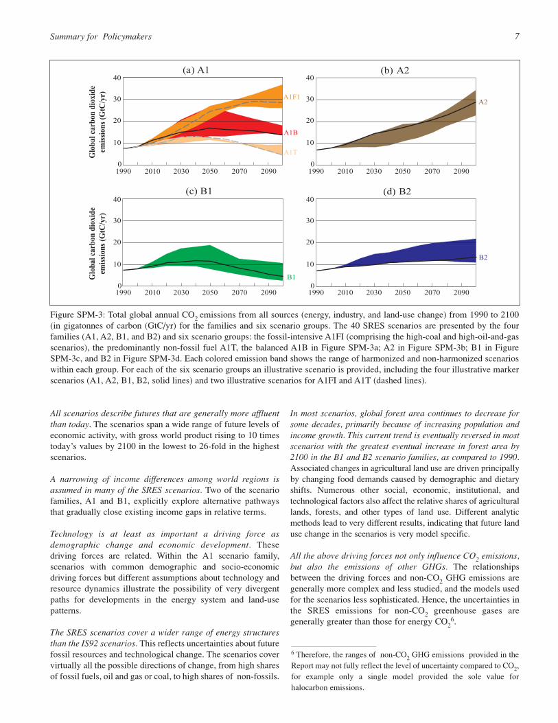
All scenarios describe futures that are generally more affluentthan today. The scenarios span a wide range of future levels ofeconomic activity, with gross world product rising to 10 timestoday’s values by 2100 in the lowest to 26-fold in the highestscenarios.
A narrowing of income differences among world regions isassumed in many of the SRES scenarios. Two of the scenariofamilies, A1 and B1, explicitly explore alternative pathwaysthat gradually close existing income gaps in relative terms.
Technology is at least as important a driving force asdemographic change and economic development. Thesedriving forces are related. Within the A1 scenario family,scenarios with common demographic and socio-economicdriving forces but different assumptions about technology andresource dynamics illustrate the possibility of very divergentpaths for developments in the energy system and land-usepatterns.
The SRES scenarios cover a wider range of energy structuresthan the IS92 scenarios. This reflects uncertainties about futurefossil resources and technological change. The scenarios covervirtually all the possible directions of change, from high sharesof fossil fuels, oil and gas or coal, to high shares of non-fossils.
In most scenarios, global forest area continues to decrease forsome decades, primarily because of increasing population andincome growth. This current trend is eventually reversed in mostscenarios with the greatest eventual increase in forest area by2100 in the B1 and B2 scenario families, as compared to 1990.Associated changes in agricultural land use are driven principallyby changing food demands caused by demographic and dietaryshifts. Numerous other social, economic, institutional, andtechnological factors also affect the relative shares of agriculturallands, forests, and other types of land use. Different analyticmethods lead to very different results, indicating that future landuse change in the scenarios is very model specific.
All the above driving forces not only influence CO2 emissions,but also the emissions of other GHGs. The relationshipsbetween the driving forces and non-CO2 GHG emissions aregenerally more complex and less studied, and the models usedfor the scenarios less sophisticated. Hence, the uncertainties inthe SRES emissions for non-CO2 greenhouse gases aregenerally greater than those for energy CO2
Figure SPM-3: Total global annual CO2 emissions from all sources (energy, industry, and land-use change) from 1990 to 2100(in gigatonnes of carbon (GtC/yr) for the families and six scenario groups. The 40 SRES scenarios are presented by the fourfamilies (A1, A2, B1, and B2) and six scenario groups: the fossil-intensive A1FI (comprising the high-coal and high-oil-and-gasscenarios), the predominantly non-fossil fuel A1T, the balanced A1B in Figure SPM-3a; A2 in Figure SPM-3b; B1 in FigureSPM-3c, and B2 in Figure SPM-3d. Each colored emission band shows the range of harmonized and non-harmonized scenarioswithin each group. For each of the six scenario groups an illustrative scenario is provided, including the four illustrative markerscenarios (A1, A2, B1, B2, solid lines) and two illustrative scenarios for A1FI and A1T (dashed lines).
6 Therefore, the ranges of non-CO2 GHG emissions provided in theReport may not fully reflect the level of uncertainty compared to CO2,for example only a single model provided the sole value forhalocarbon emissions.
Figure SPM-4: Total global cumulative CO2 emissions (GtC) from 1990 to 2100 (SPM-4a) and histogram of their distributionby scenario groups (SPM-4b). No probability of occurrence should be inferred from the distribution of SRES scenarios or thosein the literature. Both figures show the ranges of cumulative emissions for the 40 SRES scenarios. Scenarios are also groupedinto four cumulative emissions categories: low, medium–low, medium–high, and high emissions. Each category contains oneillustrative marker scenario plus alternatives that lead to comparable cumulative emissions, although often through differentdriving forces. This categorization can guide comparisons using either scenarios with different driving forces yet similaremissions, or scenarios with similar driving forces but different emissions. The cumulative emissions of the IS92 scenarios arealso shown.
0
2
4
6
8
10
12
14
16
18
Cumulative Emission 1990-2100, GtC
IS92c
Low Medium-High HighMedium-Low
600-700
800-900
1000-1100
1200-1300
1400-1500
1600-1700
1800-1900
2000-2100
2200-2300
2400-2500
NumberofScenarios
400-500
200-300
<100
A2
B1
A1B
B2
A1FIA1T
IS92d
IS92b
IS92a
IS92f
IS92e
Scenarios grouped bycumulative emissions
2600-2700
2800-2900
3000-3100
3200-3300
3400-3500
a
b
What is the range of GHG emissions in the SRES scenariosand how do they relate to driving forces?
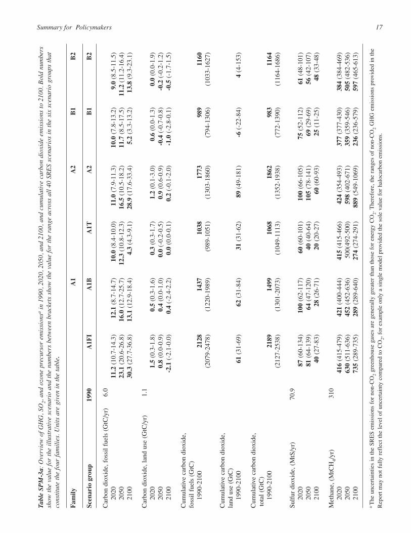
The SRES scenarios cover most of the range of carbon dioxide(CO2; see Figures SPM-2a and SPM-2b), other GHGs, andsulfur emissions found in the recent literature and SRESscenario database. Their spread is similar to that of the IS92scenarios for CO2 emissions from energy and industry as wellas total emissions but represents a much wider range for land-use change. The six scenario groups cover wide andoverlapping emission ranges. The range of GHG emissions inthe scenarios widens over time to capture the long-termuncertainties reflected in the literature for many of the drivingforces, and after 2050 widens significantly as a result ofdifferent socio-economic developments. Table SPM-2bsummarizes the emissions across the scenarios in 2020, 2050,and 2100. Figure SPM-3 shows in greater detail the ranges oftotal CO2 emissions for the six scenario groups of scenariosthat constitute the four families (the three scenario families A2,B1, and B2, plus three groups within the A1 family A1FI, A1T,and A1B).
Some SRES scenarios show trend reversals, turning points (i.e.,initial emission increases followed by decreases), andcrossovers (i.e., initially emissions are higher in one scenario,but later emissions are higher in another scenario). Emissiontrend reversals (see Figures SPM-2 and SPM-3) depart fromhistorical emission increases. In most of these cases, theupward emissions trend due to income growth is more thancompensated by productivity improvements combined with aslowly growing or declining population.
In many SRES scenarios CO2 emissions from loss of forestcover peak after several decades and then gradually decline7
(Figure SPM-1b). This pattern is consistent with scenarios inthe literature and can be associated with slowing populationgrowth, followed by a decline in some scenarios, increasingagricultural productivity, and increasing scarcity of forest land.These factors allow for a reversal of the current trend of loss offorest cover in many cases. Emissions decline fastest in the B1family. Only in the A2 family do net anthropogenic CO2emissions from land use change2 remain positive through 2100.As was the case for energy-related emissions, CO2 emissionsrelated to land-use change in the A1 family cover the widestrange. The diversity across these scenarios is amplified throughthe high economic growth, increasing the range of alternatives,and through the different modeling approaches and theirtreatment of technology.
Total cumulative SRES carbon emissions from all sourcesthrough 2100 range from approximately 770 GtC toapproximately 2540 GtC. According to the IPCC SecondAssessment Report (SAR), “any eventual stabilisedconcentration is governed more by the accumulated
anthropogenic CO2 emissions from now until the time ofstabilisation than by the way emissions change over theperiod.” Therefore, the scenarios are also grouped in the reportaccording to their cumulative emissions.8 (see Figure SPM-4).The SRES scenarios extend the IS92 range toward higheremissions (SRES maximum of 2538 GtC compared to 2140GtC for IS92), but not toward lower emissions. The lowerbound for both scenario sets is approximately 770 GtC.
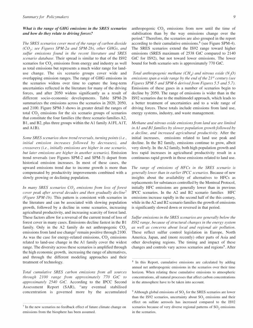
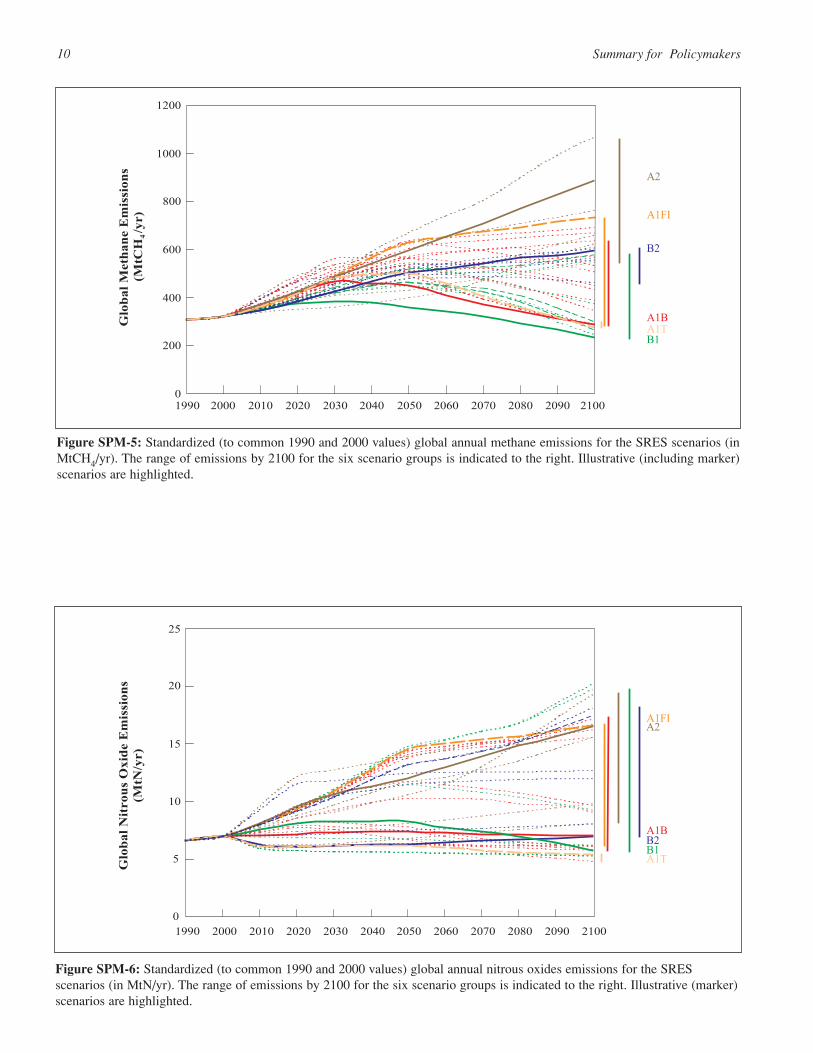
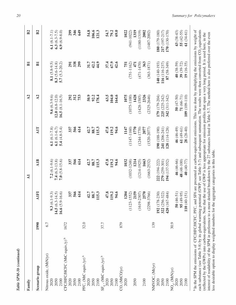
Total anthropogenic methane (CH4) and nitrous oxide (N2O)emissions span a wide range by the end of the 21st century (seeFigures SPM-5 and SPM-6 derived from Figures 5.5 and 5.7).Emissions of these gases in a number of scenarios begin todecline by 2050. The range of emissions is wider than in theIS92 scenarios due to the multimodel approach, which leads toa better treatment of uncertainties and to a wide range ofdriving forces. These totals include emissions from land use,energy systems, industry, and waste management.
Methane and nitrous oxide emissions from land use are limitedin A1 and B1 families by slower population growth followed bya decline, and increased agricultural productivity. After theinitial increases, emissions related to land use peak anddecline. In the B2 family, emissions continue to grow, albeitvery slowly. In the A2 family, both high population growth andless rapid increases in agricultural productivity result in acontinuous rapid growth in those emissions related to land use.
The range of emissions of HFCs in the SRES scenario isgenerally lower than in earlier IPCC scenarios. Because of newinsights about the availability of alternatives to HFCs asreplacements for substances controlled by the Montreal Protocol,initially HFC emissions are generally lower than in previousIPCC scenarios. In the A2 and B2 scenario families HFCemissions increase rapidly in the second half of the this century,while in the A2 and B2 scenario families the growth of emissionsis significantly slowed down or reversed in that period.
Sulfur emissions in the SRES scenarios are generally below theIS92 range, because of structural changes in the energy systemas well as concerns about local and regional air pollution.These reflect sulfur control legislation in Europe, NorthAmerica, Japan, and (more recently) other parts of Asia andother developing regions. The timing and impact of thesechanges and controls vary across scenarios and regions9. After
9Summary for Policymakers
7 In the new scenarios no feedback effect of future climate change onemissions from the biosphere has been assumed.
8 In this Report, cumulative emissions are calculated by addingannual net anthropogenic emissions in the scenarios over their timehorizon. When relating these cumulative emissions to atmosphericconcentrations, all natural processes that affect carbon concentrationsin the atmosphere have to be taken into account.
9 Although global emissions of SO2 for the SRES scenarios are lowerthan the IS92 scenarios, uncertainty about SO2 emissions and theireffect on sulfate aerosols has increased compared to the IS92scenarios because of very diverse regional patterns of SO2 emissionsin the scenarios.
Figure SPM-5: Standardized (to common 1990 and 2000 values) global annual methane emissions for the SRES scenarios (inMtCH4/yr). The range of emissions by 2100 for the six scenario groups is indicated to the right. Illustrative (including marker)scenarios are highlighted.
Figure SPM-6: Standardized (to common 1990 and 2000 values) global annual nitrous oxides emissions for the SRESscenarios (in MtN/yr). The range of emissions by 2100 for the six scenario groups is indicated to the right. Illustrative (marker)scenarios are highlighted.
initial increases over the next two to three decades, globalsulfur emissions in the SRES scenarios decrease (see TableSPM-1b), consistent with the findings of the 1995 IPCCscenario evaluation and recent peer-reviewed literature.
Similar future GHG emissions can result from very differentsocio-economic developments, and similar developments ofdriving forces can result in different future emissions.Uncertainties in the future developments of key emissiondriving forces create large uncertainties in future emissions,even within the same socio-economic development paths.Therefore, emissions from each scenario family overlapsubstantially with emissions from other scenario families. Theoverlap implies that a given level of future emissions can arisefrom very different combinations of driving forces. FiguresSPM-1, SPM-2, and SPM-3 show this for CO2.
Convergence of regional per capita incomes can lead to eitherhigh or low GHG emissions. Tables SPM-1a and SPM-1bindicate that there are scenarios with high per capita incomesin all regions that lead to high CO2 emissions (e.g., in the high-growth, fossil fuel intensive scenario group A1FI). They alsoindicate that there are scenarios with high per capita incomesthat lead to low emissions (e.g., the A1T scenario group or theB1 scenario family). This suggests that in some cases otherdriving forces may have a greater influence on GHG emissionsthan income growth.
How can the SRES scenarios be used?
It is recommended that a range of SRES scenarios with avariety of assumptions regarding driving forces be used in anyanalysis. Thus more than one family should be used in mostanalyses. The six scenario groups – the three scenario familiesA2, B1, and B2, plus three groups within the A1 scenariofamily, A1B, A1FI, and A1T – and four cumulative emissionscategories were developed as the smallest subsets of SRESscenarios that capture the range of uncertainties associatedwith driving forces and emissions.
The important uncertainties ranging from driving forces toemissions may be different in different applications – forexample climate modeling; assessment of impacts,vulnerability, mitigation, and adaptation options; and policyanalysis. Climate modelers may want to cover the rangereflected by the cumulative emissions categories. To assess therobustness of options in terms of impacts, vulnerability, andadaptation may require scenarios with similar emissions butdifferent socio-economic characteristics, as reflected by the sixscenario groups. For mitigation analysis, variation in bothemissions and socio-economic characteristics may benecessary. For analysis at the national or regional scale, themost appropriate scenarios may be those that best reflectspecific circumstances and perspectives.
There is no single most likely, “central”, or “best-guess”scenario, either with respect to SRES scenarios or to the
underlying scenario literature. Probabilities or likelihood arenot assigned to individual SRES scenarios. None of the SRESscenarios represents an estimate of a central tendency for alldriving forces or emissions, such as the mean or median, andnone should be interpreted as such. The distribution of thescenarios provides a useful context for understanding therelative position of a scenario but does not represent thelikelihood of its occurrence.
The driving forces and emissions of each SRES scenario shouldbe used together. To avoid internal inconsistencies,components of SRES scenarios should not be mixed. Forexample, the GHG emissions from one scenario and the SO2emissions from another scenario, or the population from oneand economic development path from another, should not becombined.
While recognizing the inherent uncertainties in long-termprojections10, the SRES scenarios may provide policymakerswith a long-term context for near-term analysis. The modelingtools that have been used to develop these scenarios that focuson the century time scale are less suitable for analysis of nearterm (a decade or less) developments. When analyzingmitigation and adaptation options, the user should be awarethat although no additional climate initiatives are included inthe SRES scenarios, various changes have been assumed tooccur that would require other interventions, such as thoseleading to reductions in sulfur emissions and significantpenetration of new energy technologies.
What future work on emissions scenarios would be useful?
• Establishment of a program for on-going evaluationsand comparisons of long-term emission scenarios,including a regularly updated scenario database;
• Capacity building, particularly in developing countries,in the area of modeling tools and emissions scenarios;
• Multiple storyline, multi-model approaches in futurescenario analyses;
• New research activities to assess future developmentsin key GHG driving forces in greater regional,subregional, and sectoral detail which allow for aclearer link between emissions scenarios and mitigationoptions;
• Improved specification and data for, and integration of,the non-CO2 GHG and non-energy sectors, such as landuse, land-use change and forestry, in models, as well asmodel inter-comparison to improve scenarios andanalyses;
• Integration into models emissions of particulate,hydrogen, or nitrate aerosol precursors, and processes,
11Summary for Policymakers
10 Confidence in the quantification of any scenario decreasessubstantially as the time horizon increases because the basis forthe assumptions becomes increasingly speculative. This is why aset of scenarios was developed.
such as feedback of climate change on emissions, thatmay significantly influence scenario results andanalyses;
• Development of additional gridded emissions forscenarios which would facilitate improved regionalassessment;
• Assessment of strategies that would address multiplenational, regional, or global priorities;
• Development of methods for scientifically soundaggregation of emissions data;
• More detailed information on assumptions, inputs, andthe results of the 40 SRES scenarios should be madeavailable at a web site and on a CD-ROM. Regularmaintenance of the SRES web site is needed;
• Extension of the SRES web site and production of aCD-ROM to provide, if appropriate, time-dependentgeographic distributions of driving forces andemissions, and concentrations of GHGs and sulfateaerosols.
• Development of a classification scheme for classifyingscenarios as intervention or non-intervention scenarios.


![[Table S ummary] Xinjiang Plant to Drive Cost Lower ...](https://static.documents.pub/doc/80x56/625863ca2894776b1e69ee99/table-s-ummary-xinjiang-plant-to-drive-cost-lower-.jpg)


