UNCERTAINTIES AND MULTIDISCIPLINARY …user.engineering.uiowa.edu/~kkchoi/D_RBDO_B.06.pdf · ·...

Choi, K.K., Youn, B.D., Tang, J., Freeman, J., Stadterman, T., Connon, W., and Peltz, A., “Integrated Computer-Aided Engineering Methodology for Various Uncertainties and Multidisciplinary Applications,” Engineering Design Reliability Handbook, CRC Press, 2004.

1

INTEGRATED COMPUTER-AIDED ENGINEERING METHODOLOGY FOR VARIOUS

UNCERTAINTIES AND MULTIDISCIPLINARY APPLICATIONS

Kyung K. Choi1, Byeng D. Youn2, Jun Tang3

Center for Computer-Aided Design and Department of Mechanical and Industrial Engineering College of Engineering, The University of Iowa

Iowa City, IA 52242

Jeffrey S. Freeman4

Department of Mechanical Engineering The University of Tennessee Knoxville, TN 37996-2210

Thomas J. Stadterman5, Alan L. Peltz6

US Army Materiel Systems Analysis Activity (AMSAA) Aberdeen Proving Ground, MD 21005-5071

William (Skip) Connon7, US Army Aberdeen Test Center

400 Colleran Rd. Aberdeen Proving Ground, MD 21005-5059

1 Carver Professor, e-mail: [email protected] Assistant Research Engineer, e-mail: [email protected] Research Scientist, e-mail: [email protected] Associate Professor, e-mail: [email protected] Physics-of-Failure Team Leader, e-mail: [email protected] Mechanical Engineer, e-mail: [email protected] Mechanical Engineer, e-mail: [email protected]

mailto:[email protected]








2

KEYWORDS

Computer-Aided Engineering (CAE); Reliability-Based Design; Experiment; Durability;

Uncertainty

NOMENCLATURE

L Crack initiation fatigue life

W Weight for design optimization

d Design parameter; d = [d1, d2,…, dn]T

g(d) design constraint of design parameters

X Random vector; X = [X1, X2,…, Xn]T

x Realization of X; x = [x1, x2,…, xn]T

G(X) Constraint of random parameters

U Independent and standard normal random parameter

u Realization of U; u = [u1, u2,…, un]T

Pf Probability of failure

fX Probability density function of X

µ Mean of random vector X; µ = [µ1, µ2,…, µn]T

β Reliability index

fK Fatigue-strength reduction factor

tK Stress intensification factor

q Notch sensitivity factor

1. INTRODUCTION

Given the explosive growth in computational technology, computer-aided engineering (CAE)

has long been used to analyze and evaluate product design. However, various uncertainties in an


3

engineering system prevent CAE from being directly used for such purposes. Through the use of

experimental validation and probabilistic methods, CAE will become an integral part of

engineering product analysis and design. This chapter presents an advanced CAE methodology

for qualitative, reliable, durable, and/or cost-effective product design under uncertainty that is

composed of three key elements: CAE technology, experimental validation, and an uncertainty-

based design [1-5].

CAE technology, such as simulation techniques, enables one to explore many different designs

without building expensive prototype models. As shown in Fig. 1, one must inevitably take

account of physical input uncertainties, such as geometric dimensions, material properties, and

loads. However, a simulation (or mathematical) model that departs from a prototype model

introduces modeling uncertainty, uncertainty due approximations in numerical algorithms, in

addition to any inherent physical uncertainty in the structure. It is not possible to completely

eliminate model uncertainty but this could be expensive. Instead it could be more practical to

minimize modeling uncertainty through experimental validation. Moreover, while modeling

physical uncertainty, a lack of statistical information may lead to statistical uncertainty, such as

uncertainty of the distribution type and its parameters, which could be modeled using Bayesian

probability or possibility or evidence theory [6,7]. In fact, any engineering uncertainty can be

categorized within three general types: physical uncertainty, model uncertainty, and statistical

uncertainty [8].

Figure 1. Uncertainty Types Existing in Computer-Aided Design


4

Therefore, an integrated CAE methodology is presented along with experimental validation and

an uncertainty-based design, as shown in Fig. 2. Assuming that statistical uncertainty is minimal

with enough statistical information, an advanced CAE methodology can be presented with

experimental validation and reliability-based design. As a result, a high fidelity model and

analysis can be created that takes physical and model uncertainties into account.

Figure 2. Integrated Computer-Aided Engineering Methodology

Mechanical fatigue subject to external and inertia transient loads in the service life of a

mechanical system often leads to structural failure due to accumulated damage [9]. A structural

durability analysis that predicts the fatigue life of a mechanical component subject to dynamic

stresses and strains is an intensive and complicated multidisciplinary simulation process, since it

requires the integration of several CAE tools and a large amount of data communication and

computation. Uncertainties in geometric dimensions and material properties due to

manufacturing tolerances result in indeterministic nature of fatigue life for the mechanical

component. The main objective of this chapter is thus to demonstrate the possibilities of

advanced CAE methodology for structural durability with experimental validation and

reliability-based design. In this way, it can be ascertained whether the modeling and simulation

is feasible and an optimal design is reliable. One of the primary challenges in developing an

integrated CAE methodology is to produce effective reliability-based design optimization

(RBDO) methods [1,4,5].


5

2. FATIGUE LIFE ANALYSIS AND EXPERIMENTAL VALIDATION

2.1 Mechanical Fatigue Failure for Army Trailer Drawbar

As shown in Fig. 3, the Army trailer encounters a mechanical failure due to damage

accumulation after driving 1,671 miles on the Perryman course #3 at a constant speed of 15

miles per hour. This research thus initiates a physics of failure model of the Army trailer

through the validation of the simulation model, dynamic analysis, and durability analysis, further

improving the trailer’s design to extend its overall fatigue life and minimize its weight.

Figure 3. Army Trailer and Its Structural Failure

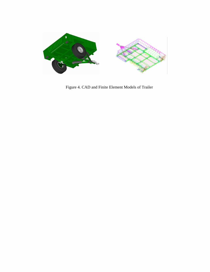
2.2 Experimental Validation of Mechanical Fatigue

2.2.1 Validation of Simulation Model

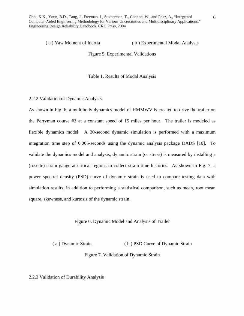
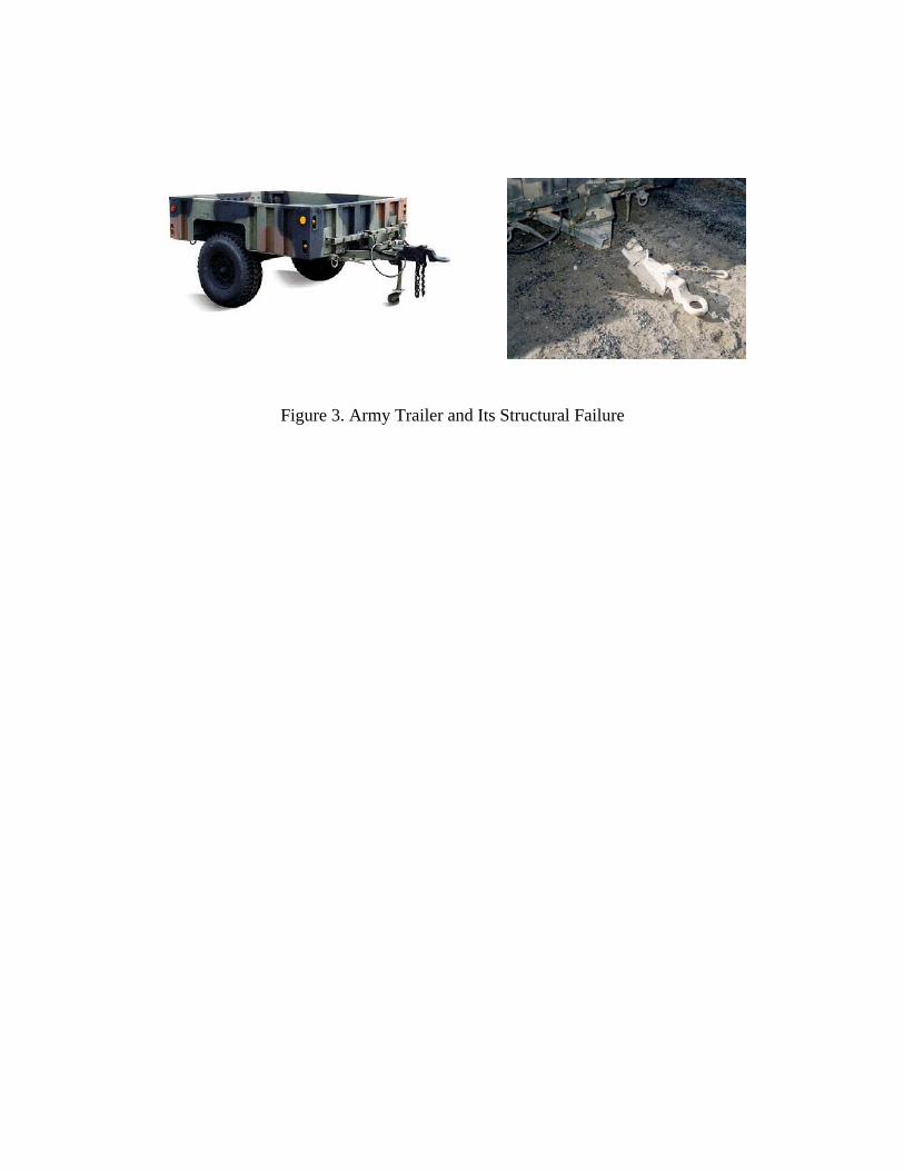
As shown in Fig. 4, the computer-aided design (CAD) model for the US Army trailer is

developed with Pro/Engineer to simulate a real trailer model. To achieve high fidelity of the

CAD model, the CAD model goes through an experimental validation, which includes

comparison of the mass/inertia properties and the natural frequencies and mode shapes of the

model with measurements.

Figure 4. CAD and Finite Element Models of Trailer

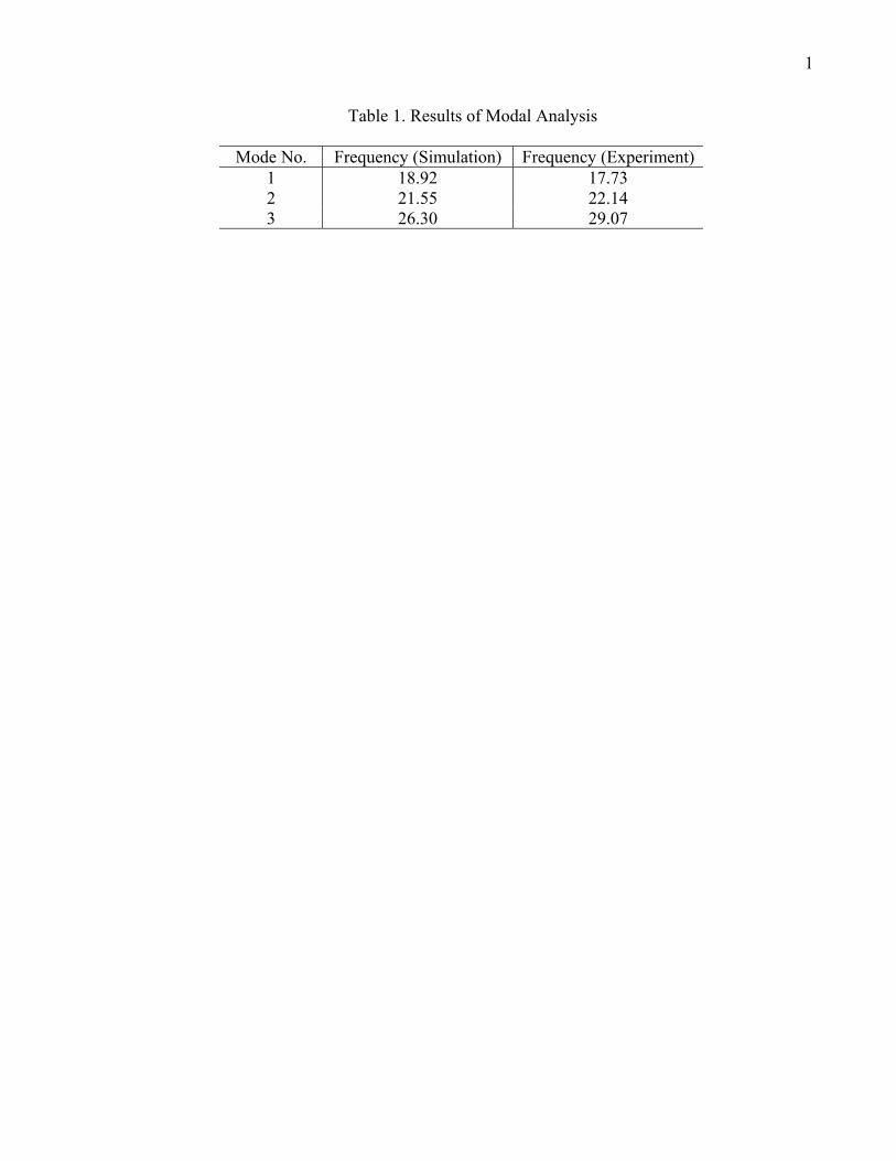
Results of the modal analysis are shown in Table 1, indicating that simulation results are close to

experimental results. Meanwhile, other mechanical components, such as a tire, axle, shock

absorber, etc. are appropriately modeled through experimental validation.


6

( a ) Yaw Moment of Inertia ( b ) Experimental Modal Analysis

Figure 5. Experimental Validations

Table 1. Results of Modal Analysis

2.2.2 Validation of Dynamic Analysis

As shown in Fig. 6, a multibody dynamics model of HMMWV is created to drive the trailer on

the Perryman course #3 at a constant speed of 15 miles per hour. The trailer is modeled as

flexible dynamics model. A 30-second dynamic simulation is performed with a maximum

integration time step of 0.005-seconds using the dynamic analysis package DADS [10]. To

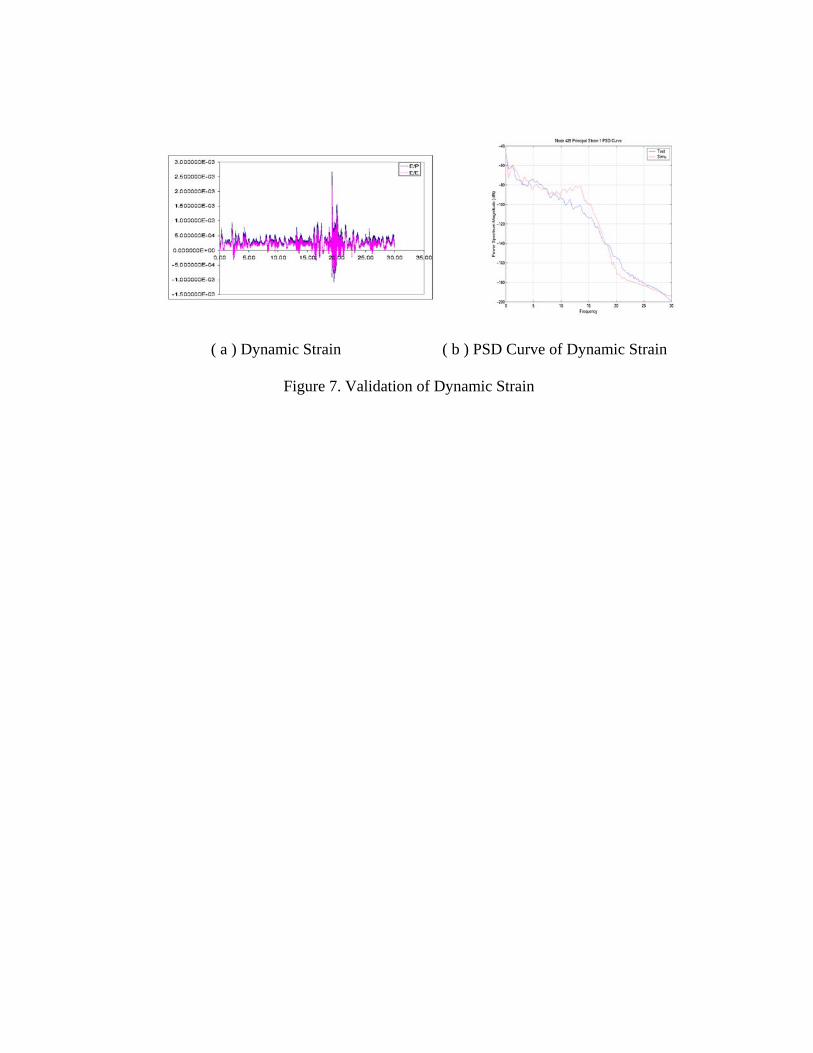
validate the dynamics model and analysis, dynamic strain (or stress) is measured by installing a

(rosette) strain gauge at critical regions to collect strain time histories. As shown in Fig. 7, a

power spectral density (PSD) curve of dynamic strain is used to compare testing data with

simulation results, in addition to performing a statistical comparison, such as mean, root mean

square, skewness, and kurtosis of the dynamic strain.

Figure 6. Dynamic Model and Analysis of Trailer

( a ) Dynamic Strain ( b ) PSD Curve of Dynamic Strain

Figure 7. Validation of Dynamic Strain

2.2.3 Validation of Durability Analysis


7

Figure 8. Computation Process for Fatigue Life

For a durability analysis, the fatigue life for crack initiation is calculated at those critical regions

in the mechanical system that experience a short life span. The fatigue life computation consists

of two primary computations, as shown in Fig. 8, for dynamic stress and fatigue life. Dynamic

stress can be obtained from either a hardware prototype experiment in which mounting sensors

or transducers are placed on the physical component, or from numerical simulation. Using

simulation, a stress influence coefficient (SIC) [11] obtained from quasi-static finite element

analysis (FEA) using MSC NASTRAN is superposed with dynamic analysis results, including

external forces, accelerations, and angular velocities, to compute the dynamic stress history.

This history is then used to compute the crack initiation fatigue life of the component.

Durability analysis is carried out using durability analysis and reliability workspace (DRAW)

programs developed at the University of Iowa [11]. A preliminary durability analysis is

executed to estimate the fatigue life of the Army trailer and to predict the critical regions that

experience a low fatigue life. The critical regions on the drawbar assembly are clearly shown in

Fig. 9, excluding any fictitious critical regions that are the result of modeling imperfections due

to applied boundary conditions. To compute the multiaxial crack initiation life of the roadarm,

the equivalent von Mises strain approach is employed, which is described by the fatigue

resistance and cyclic strength of the material as [12]

(2 ) (2 ) and ( )2

f b cf f f pN N K

Enσε ε σ ε ′′∆ ′= + = ′ (1)


8

, , , , ,b c K nwith the empirical constants (σ ε′ ′ ′ ′ ). Details on durability analysis are discussed in

Refs. 11 and 12.

Figure 9. Fatigue Life Contour of Army Trailer Drawbar

2.3 Design Optimization for Mechanical Fatigue

Since damage accumulation leads to structural fatigue failure in the drawbar assembly, durability

design optimization for the Army trailer drawbar is carried out to improve its fatigue life and to

minimize weight. The critical region where mechanical fatigue failure occurs is now taken into

account in conducting the design optimization process. The integrated design optimization

process involves: (a) design parameterization [13], (b) design sensitivity analysis (DSA) [13],

and (c) design optimization [14]. Design parameters of the drawbar assembly are carefully

defined, taking geometric and manufacturing restrictions into account.

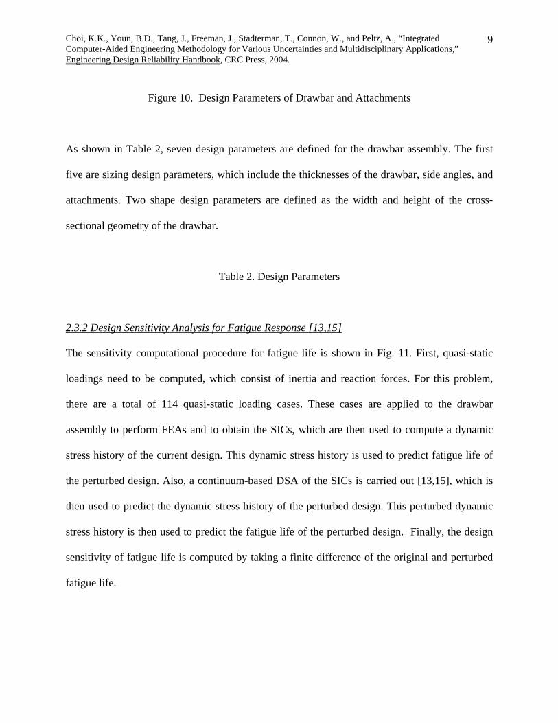
2.3.1 Design Parameterization

As shown in Fig. 10, the drawbar assembly is composed of one central bar, two side bars, six

side angles, two side attachments, and top and bottom plates. The optimum design of the

drawbar assembly needs to be symmetric, and thus, design parameterization is made to yield a

symmetric design. Bars and attachments at the initial design have a uniform thickness.

However, the thicknesses of those elements of the drawbar assembly that can be changed during

the design optimization process are modeled as sizing design parameters. While maintaining the

rectangular shape of the central and side bars, their height and width are considered as shape

design parameters.


9

Figure 10. Design Parameters of Drawbar and Attachments

As shown in Table 2, seven design parameters are defined for the drawbar assembly. The first

five are sizing design parameters, which include the thicknesses of the drawbar, side angles, and

attachments. Two shape design parameters are defined as the width and height of the cross-

sectional geometry of the drawbar.

Table 2. Design Parameters

2.3.2 Design Sensitivity Analysis for Fatigue Response [13,15]

The sensitivity computational procedure for fatigue life is shown in Fig. 11. First, quasi-static

loadings need to be computed, which consist of inertia and reaction forces. For this problem,

there are a total of 114 quasi-static loading cases. These cases are applied to the drawbar

assembly to perform FEAs and to obtain the SICs, which are then used to compute a dynamic

stress history of the current design. This dynamic stress history is used to predict fatigue life of

the perturbed design. Also, a continuum-based DSA of the SICs is carried out [13,15], which is

then used to predict the dynamic stress history of the perturbed design. This perturbed dynamic

stress history is then used to predict the fatigue life of the perturbed design. Finally, the design

sensitivity of fatigue life is computed by taking a finite difference of the original and perturbed

fatigue life.


10

2.3.3 Durability Design Optimization

The design objective is to increase the fatigue life of the drawbar, while minimizing the weight

of the Army trailer drawbar assembly. Due to restrictions placed on manufacturing and

assembling processes, side constraints are generally imposed on the design parameters.

Figure 11. Computational Procedure for Design Sensitivity Analysis of Flexible Structural

Systems

Therefore, the design optimization problem can be formulated as

min

Minimize ( )Subject to 1 ( ) 0, 1, ,

,i iL U n

Wg L L i n

dv

c

R

= − ≤ =

≤ ≤ ∈

dd

d d d d

… (2)

where W(d) is the weight of the drawbar assembly, Li(d) is the fatigue life at the ith node, Lmin is

the required minimum fatigue life, gi is the ith design constraint, and dl and du are lower and

upper bounds of the design parameters, respectively. In Eq. (2), nc is the number of design

constraints, and ndv is the number of design parameters.

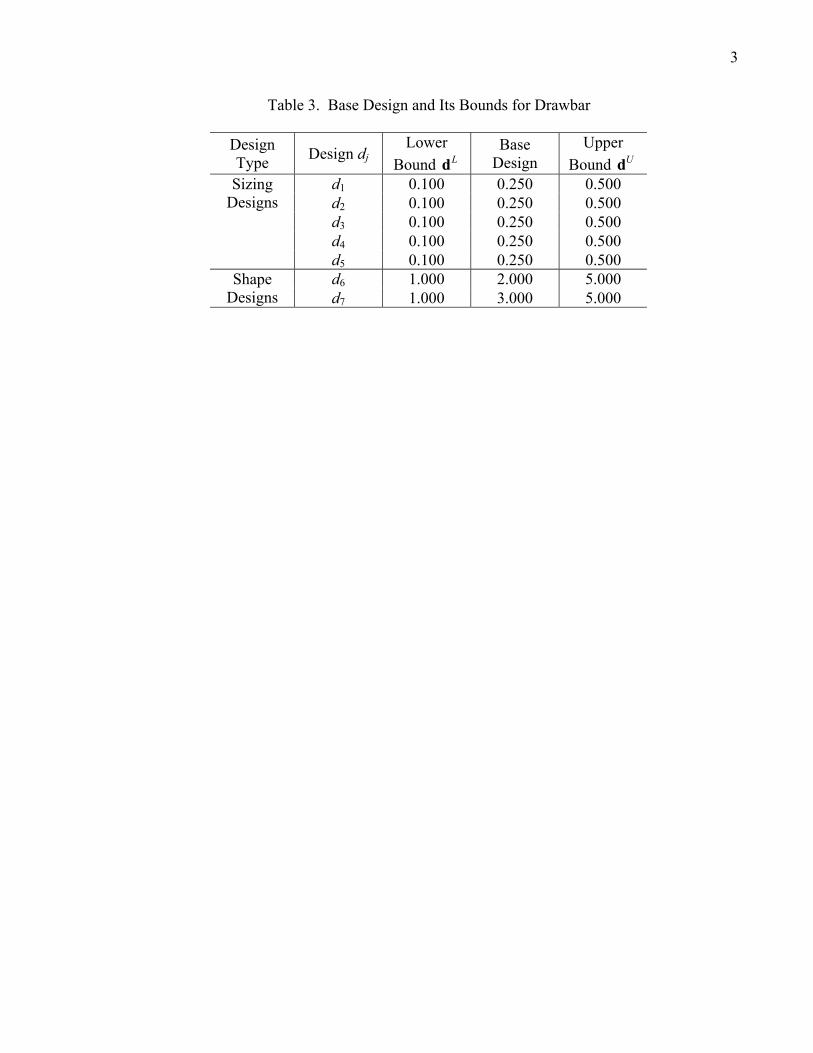
For the seven design parameters (ndv=7) defined in Table 2, the base design and design bounds

are shown in Table 3. The side constraints need to be set by considering the restriction of

manufacturing and assembling processes. For example, it is not possible for any upper bound of

the sizing design parameter to be larger than half the size of a lower bound in the corresponding

shape design parameter in the same cross-section.

Table 3. Base Design and Its Bounds for Drawbar


11

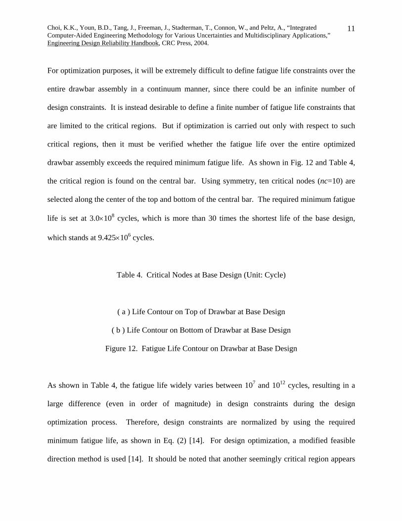
For optimization purposes, it will be extremely difficult to define fatigue life constraints over the

entire drawbar assembly in a continuum manner, since there could be an infinite number of

design constraints. It is instead desirable to define a finite number of fatigue life constraints that

are limited to the critical regions. But if optimization is carried out only with respect to such

critical regions, then it must be verified whether the fatigue life over the entire optimized

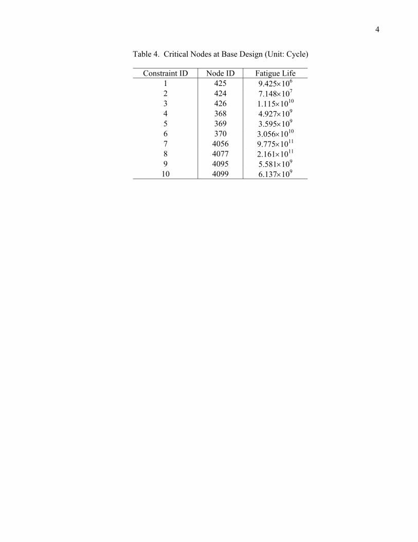
drawbar assembly exceeds the required minimum fatigue life. As shown in Fig. 12 and Table 4,

the critical region is found on the central bar. Using symmetry, ten critical nodes (nc=10) are

selected along the center of the top and bottom of the central bar. The required minimum fatigue

life is set at 3.0×108 cycles, which is more than 30 times the shortest life of the base design,

which stands at 9.425×106 cycles.

Table 4. Critical Nodes at Base Design (Unit: Cycle)

( a ) Life Contour on Top of Drawbar at Base Design

( b ) Life Contour on Bottom of Drawbar at Base Design

Figure 12. Fatigue Life Contour on Drawbar at Base Design

As shown in Table 4, the fatigue life widely varies between 107 and 1012 cycles, resulting in a

large difference (even in order of magnitude) in design constraints during the design

optimization process. Therefore, design constraints are normalized by using the required

minimum fatigue life, as shown in Eq. (2) [14]. For design optimization, a modified feasible

direction method is used [14]. It should be noted that another seemingly critical region appears


12

at the tip of the drawbar on the base design. However, due to the boundary condition imposed at

the tip of the drawbar, this region is fictitious.

2.3.4 Results of Design Optimization

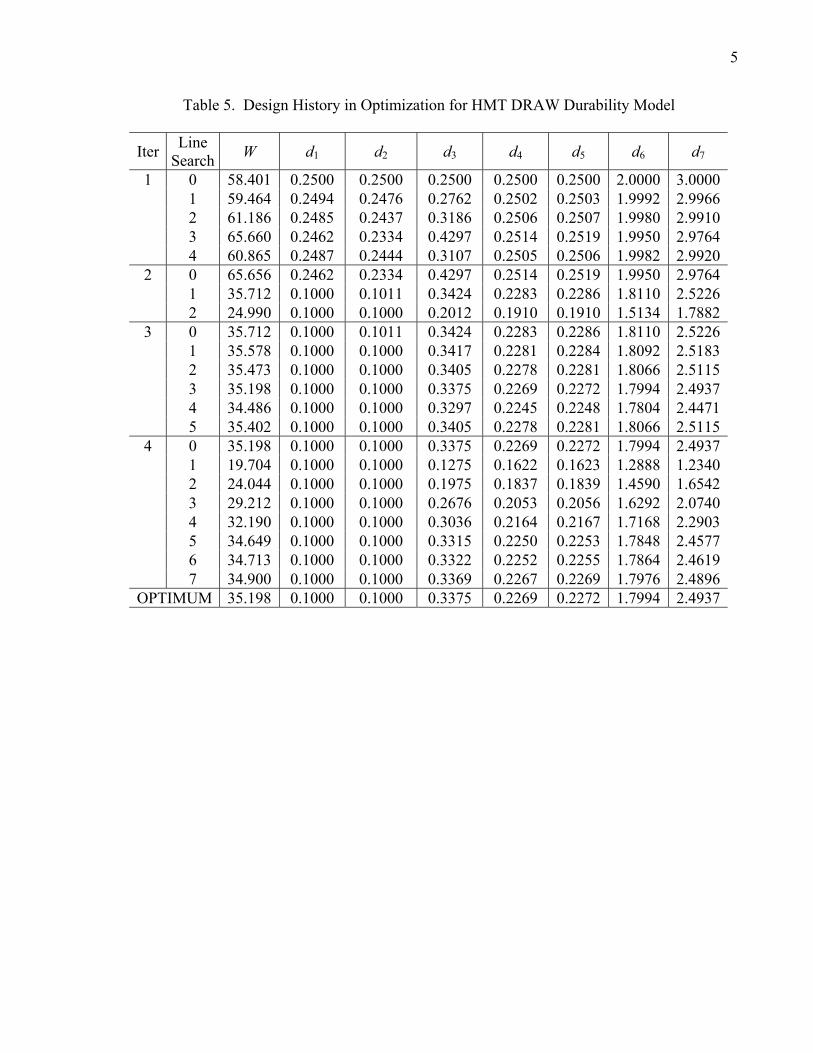
As shown in Table 5, the optimum design is obtained in four iterations. The total mass is

reduced by about 40% of its original size (from 58.401 to 35.198 lb), while all fatigue life

constraints are satisfied. As shown in Fig. 12, the critical region at the base design is spread out

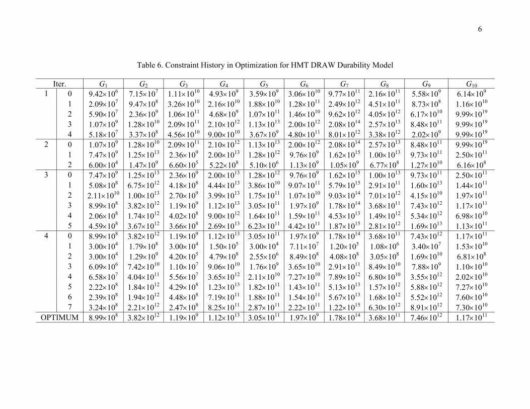
over the front of the central bar. Among ten design constraints, only the first and second

constraints (at nodes 425 and 424) are violated or active at the base design. On the other hand, at

the optimum design, the first, third, and sixth design constraints (nodes 425, 426, and 370)

appear to be active, as shown in Table 6.

At the optimum design, all thicknesses decrease except for the central bar, and the width and

height of all bars, which become smaller. Due to the decrease in some sizing design parameters

and both shape parameters, about 40% of the mass is saved. The first two design parameters, b1

and b2, decrease slowly at the beginning of the optimization process, and then rapidly decrease to

the lower bound, since more rigid side bars and angles penalize the central bar, resulting in a

decrease in its fatigue life. Moreover, increasing the thickness of the central bar by 35% (d3:

from 0.25 to 0.3375 in) it further reinforces its strength and produces a longer fatigue life. At the

optimum design, the fourth and fifth design parameters (triangle plates and side attachments) are

reduced by about 9%, since the weight can be effectively reduced while the fatigue lives at

critical regions are not reduced significantly. With respect to shape design parameters, the width


13

and height are reduced by about 10% and 17%, respectively. Such design changes are

summarized in Table 7.

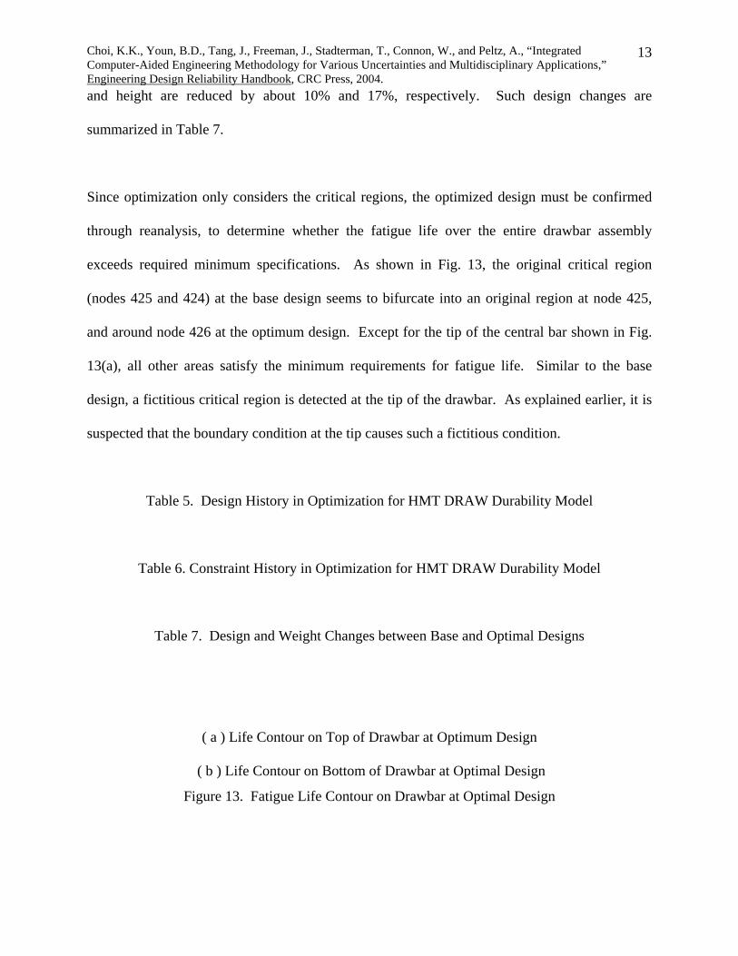
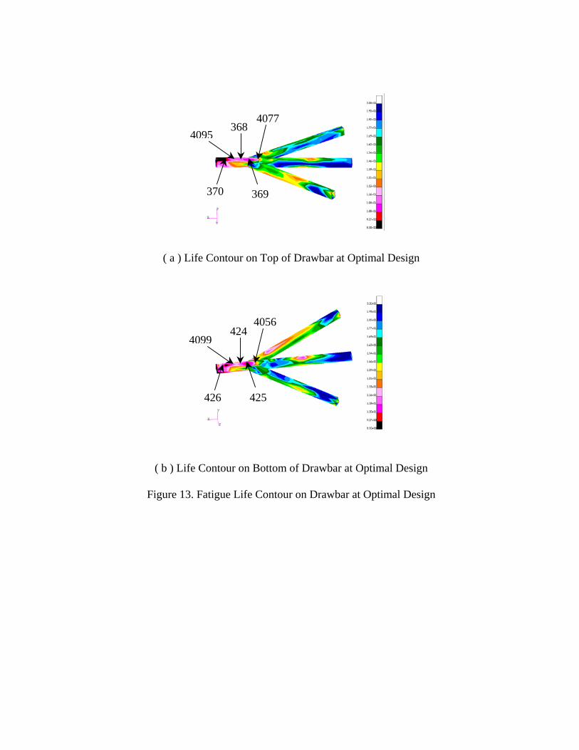
Since optimization only considers the critical regions, the optimized design must be confirmed

through reanalysis, to determine whether the fatigue life over the entire drawbar assembly

exceeds required minimum specifications. As shown in Fig. 13, the original critical region

(nodes 425 and 424) at the base design seems to bifurcate into an original region at node 425,

and around node 426 at the optimum design. Except for the tip of the central bar shown in Fig.

13(a), all other areas satisfy the minimum requirements for fatigue life. Similar to the base

design, a fictitious critical region is detected at the tip of the drawbar. As explained earlier, it is

suspected that the boundary condition at the tip causes such a fictitious condition.

Table 5. Design History in Optimization for HMT DRAW Durability Model

Table 6. Constraint History in Optimization for HMT DRAW Durability Model

Table 7. Design and Weight Changes between Base and Optimal Designs

( a ) Life Contour on Top of Drawbar at Optimum Design

( b ) Life Contour on Bottom of Drawbar at Optimal Design

Figure 13. Fatigue Life Contour on Drawbar at Optimal Design


14

2.3.5 Results of Design Optimization Considering Notch Effects [17]

Having identified the region near node 425 on the trailer drawbar as the location of the shortest

fatigue life, it is now necessary to apply the fatigue-strength reduction factor (Kf) to account for

the effect of geometric discontinuities in the critical region, as shown in Table 8. A fatigue-

strength reduction factor reduces the predicted fatigue life in a manner proportional to the

severity of the geometric discontinuity. Kf is calculated from the stress intensity factor Kt and the

notch sensitivity factor q. Based on references in the literature [17], the values of Kt and q were

estimated, and the associated Kf values were calculated to be 2.6. Using this Kf, the fatigue life

on Perryman #3 course is estimated to be 9,580 miles, which means that a fatigue crack will not

initiate and grow to a 2 mm length until the trailer traverses 9,580 miles of Perryman course #3

at 15 mph, or 638 hours of continuous running. In contrast, the fatigue life of the base design

was 180 miles or 12 hours. This means that the fatigue life of the optimum design is 53.2 times

greater than that of the base design. In this example we have tried to reduce the weight of the

drawbar by imposing the constraint that the fatigue life be approximately equal to 30 times that

of the baseline design (see formulation 1). Greater increase in fatigue life could be achieved if

the fatigue life were constrained to be equal to that of the base line.

Table 8. Fatigue Life w/o and w/ Considering Notch Effects

3. RELIABILITY ANALYSIS AND RELIABILITY-BASED DESIGN OPTIMIZATION

3.1 Reliability Analysis for Durability-Based Optimal Design

The reliability analysis of the durability-based optimum design is carried out to estimate the

probability of failure as


15

8

8

3 10( 3 10 cycles) ( )

LP L f d

< ×

< × = ∫ ∫ X x x (3)

For the reliability analysis, uncertainty of each design parameter is modeled with normal

distribution and 10% coefficient of variation. The optimal design turns out to be unreliable with

a 49.7% (β=0.073) probability of failure through the reliability analysis. Considering the

variability of the design that lies on the design constraint boundaries, as shown in Fig. 14, it is

reasonable that the deterministic optimal design has only about 50% reliability. Due to the fact

that the deterministic optimal design is unreliable, it is necessary to perform a reliability-based

design optimization (RBDO) [1-5] for reliable and durable designs. Among all random

parameters, uncertainty in the 3rd random parameter (central bar thickness) has the most

significant effect on the probability of failure. Thus, without a new reliability-based optimum

design, the thickness of the central bar must be manufactured more accurately to increase

reliability, which will significantly increase the manufacturing cost.

3.2 Reliability-Based Design Optimization for Durability

As seen in the previous section, deterministic design optimization due to various uncertainties in

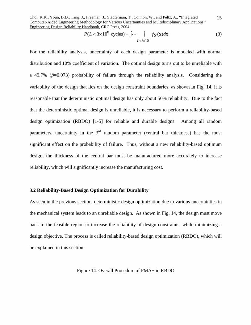
the mechanical system leads to an unreliable design. As shown in Fig. 14, the design must move

back to the feasible region to increase the reliability of design constraints, while minimizing a

design objective. The process is called reliability-based design optimization (RBDO), which will

be explained in this section.

Figure 14. Overall Procedure of PMA+ in RBDO


16

3.2.1 RBDO Model of Performance Measure Approach (PMA)

For any engineering application, the RBDO model [1-5,18-20] can generally be formulated as

(4)

where is the design vector,

minimize Cost( )subject to ( ( ( )) 0) ( ) 0, 1, 2, ,

≤ −Φ ≥ =

≤ ≤

dd X

d d di t

L U

P G i ncβ

[ ] ( )T ndvd R= = ∈d µ X [ ]T nrvi iX R= ∈

( ) ( )• ≥ Φ tP

X is the random vector, and

ndv, nrv and nc are the numbers of design parameters, random parameters, and probabilistic

constraints, respectively. The probabilistic constraints are described by a probability constraint

β for a safe event ( ( )) 0≤d XiG

( ( ))i d X

)

.

The statistical description of the failure of the performance function G is characterized

by the cumulative distribution function (iGF • as

( ( ) (0) ( )) 0≤ = ≥ Φi G tP G FXi

β (5)

where the reliability of failure is described as

(6)

In Eq. (6) is the joint probability density function of all random parameters. Its evaluation

requires a reliability analysis where multiple integrations are involved, as shown in Eq. (6).

Some approximate probability integration methods have been developed to provide efficient

solutions, such as the first-order reliability method (FORM) [1-5,8], or the asymptotic second-

order reliability method (SORM) [21,22] with a rotationally invariant measure as the reliability.

FORM often provides adequate accuracy and is widely used for design applications. In FORM,

the reliability analysis requires a transformation T [23,24] from the original random parameter X

to the standard normal random parameter U. The performance function G in X-space can

1( ) 0(0) ( ) , 1, 2,

i iG G

F f dx dx i≤

= ∫ ∫ XXx …

)x

( )X

,n nc=

(fX


17

then be mapped onto G(T(X)) ≡ G(U) in U-space.

The probabilistic constraint in Eq. (5) can be expressed as a performance measure through the

inverse transformation of as [1, 3-5,18-20]:

( )GF •

1( ( )) ( ( )) 0−= Φ ≤d Xi ip G tG F β (7)

where ipG is the ith probabilistic constraint. In Eq. (7), the probabilistic constraint in Eq. (4) can

be replaced with the performance measure. This is referred to as the performance measure

approach (PMA) [1,3-5,18-20]. Thus, the RBDO model using PMA can be redefined as

(8)

3.2.2 Reliability Analysis Model of PMA [1,5,18-20]

Reliability analysis in PMA can be formulated as the inverse of reliability analysis in the

reliability index approach. The first-order probabilistic performance measure is

obtained from a nonlinear optimization problem in U-space, defined as

minimize Cost( )subject to ( ( )) 0, 1, 2, ,

ip

L U

G i≤ =

≤ ≤

dd X

d d d

nc

,FORMpG

maximize ( )subject to =

UU t

Gβ

(9)

where the optimum point on the target reliability surface is identified as the most probable point

(MPP) *tβ β=u with a prescribed reliability *

tt β ββ == u . Unlike RIA, only the direction vector

* *t tβ β β β= =u u needs to be determined by exploring the spherical equality constraint tβ=U .

General optimization algorithms can be employed to solve the optimization problem in Eq. (9).


18

However, a hybrid mean value (HMV) first-order method is well suited for PMA due to its

stability and efficiency [1,3-5,18-20].

3.2.3 Reliability Analysis Tools for PMA

Three numerical methods [1,3-5,18-20,25] for PMA were used to solve Eq. (9): the advanced

mean value method [24] in Eq. (10), the conjugate mean value method [1,3-5,18-20] in Eq. (11),

and the hybrid mean value (HMV) method [1,3-5,18-20] in Eq. (12).

( )

(1) ( 1) ( ) ( ) AMVAMV AMV AMV AMV ( )

AMV

(( ), ( ) where ( )( )

+ ∇= = =

∇

uu n 0 u n u n uu

kk k k U

i i kU

GG

β β ) (10)

(0) (1) (1) (2) (2)CMV CMV AMV CMV AMV

( ) ( 1) ( 2) ( )( 1) ( )CMV CMV CMV CMVCMV CMV( ) ( 1) ( 2) ( )

CMV CMV CMV CMV

, , ,

( ) ( ) ( ) ( for 2 where ( )( ) ( ) ( ) ( )

− −+

− −

= = =

+ + ∇= ≥

+ + ∇

u 0 u u u u

n u n u n u uu nn u n u n u u

k k k kk k U

i k k k kU

GkG

β )=u

k

k

(11)

(12)

Although the advanced mean value method performs well for the convex performance function

in PMA, it was found to have some numerical shortcomings, such as slow convergence, or even

divergence, when applied to the concave performance function. To overcome this difficulty, the

conjugate mean value method was proposed [1,3-5,18-20]. The conjugate steepest descent

direction significantly improves the rate of convergence as well as stability, as compared to the

advanced mean value method for the concave performance function. However, the conjugate

mean value method is not as efficient as the advanced mean value method for the convex

( 1) ( ) ( 1)AMV HMV( 1)

HMV ( 1) ( ) ( 1)CMV HMV

( 1) ( 1) ( ) ( ) ( 1)

( 1)

in Eq. (8), if ( ) is convex or sign( ) 0

in Eq. (9), if ( ) is concave or sign( ) 0

with ( ) ( )

sign( ) 0 : Conve

k kk

k k

k k k k k

k

G

G

ς

ς

ς

ς

+ ++

+ +

+ + −

+

⎧ >⎪= ⎨≤⎪⎩

= − ⋅ −

>

u uu

u u

n n n n( 1)HMV( 1)HMV

x type at w.r.t. design

0 : Concave type at w.r.t. design

k

k

+

+≤

u d

u d


19

function. Consequently, the hybrid mean value (HMV) method was proposed to attain both

stability and efficiency in the MPP search for PMA [1,3-5,18-20]. The HMV method employs

the criterion for the performance function type near the MPP. Once the performance function

type is identified, either the advanced mean value or conjugate mean value method is adaptively

selected for the MPP search. The numerical procedure of the HMV method is presented with

some numerical examples in Ref. 1.

3.3 Results of Reliability-Based Shape Design Optimization for Durability of M1A1 Tank

Roadarm [14]

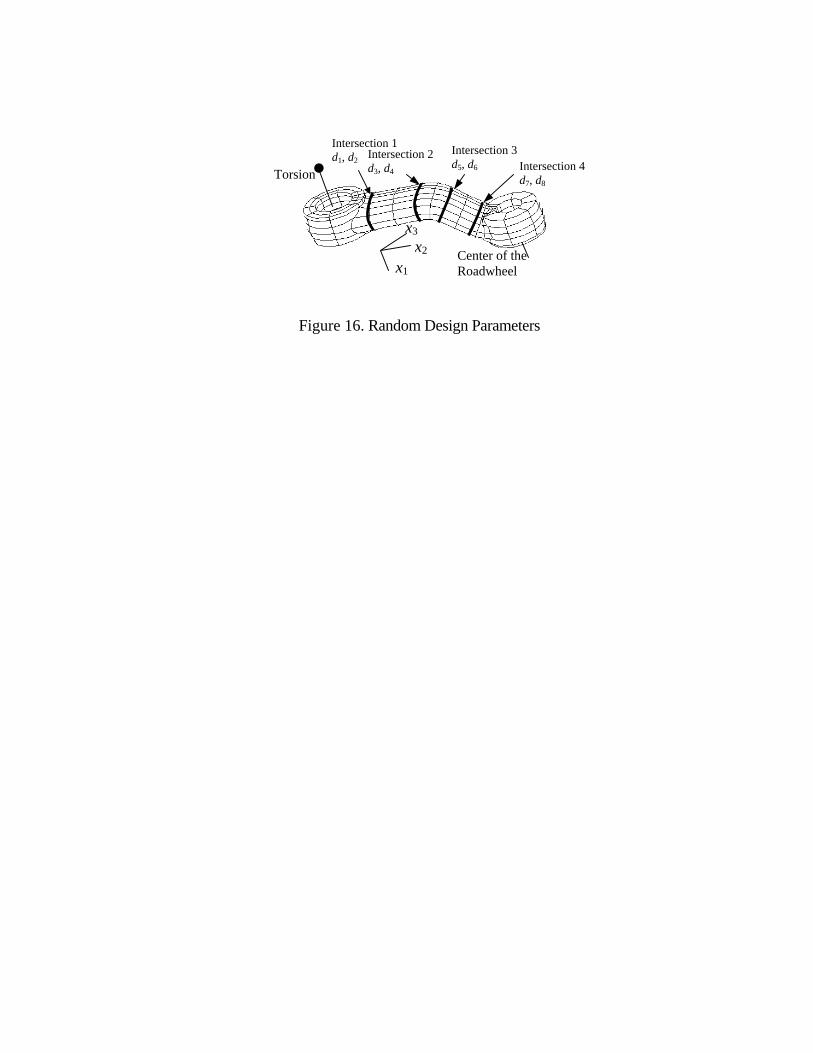
A roadarm of the military tracked vehicle shown in Fig. 15 is employed to demonstrate the

effectiveness of PMA for a large-scale RBDO application. A 17-body dynamics model is created

to simulate the tracked vehicle driven on the Aberdeen Proving Ground 4 at a constant speed of

20 miles per hour. A 20-second dynamic simulation is performed with a maximum integration

time step of 0.05-second using the dynamic analysis package DADS.

Figure 15. Military Tracked Vehicle

Figure 16. Random Design Parameters

Roadarm

As shown in Fig. 16, three hundred and ten 20-node isoparametric FEs (STIF95) and four beam

elements (STIF4) of ANSYS are used to create the roadarm finite element model, which is made

of S4340 steel. FE analysis is performed to obtain the stress influence coefficient of the roadarm

using ANSYS by applying 18 quasi-static loads. The empirical constants ( , , , , ,b c K nσ ε′ ′ ′ ′ ) for


20

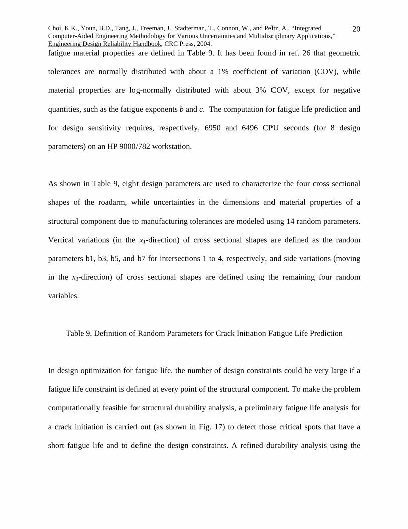
fatigue material properties are defined in Table 9. It has been found in ref. 26 that geometric

tolerances are normally distributed with about a 1% coefficient of variation (COV), while

material properties are log-normally distributed with about 3% COV, except for negative

quantities, such as the fatigue exponents b and c. The computation for fatigue life prediction and

for design sensitivity requires, respectively, 6950 and 6496 CPU seconds (for 8 design

parameters) on an HP 9000/782 workstation.

As shown in Table 9, eight design parameters are used to characterize the four cross sectional

shapes of the roadarm, while uncertainties in the dimensions and material properties of a

structural component due to manufacturing tolerances are modeled using 14 random parameters.

Vertical variations (in the x1-direction) of cross sectional shapes are defined as the random

parameters b1, b3, b5, and b7 for intersections 1 to 4, respectively, and side variations (moving

in the x3-direction) of cross sectional shapes are defined using the remaining four random

variables.

Table 9. Definition of Random Parameters for Crack Initiation Fatigue Life Prediction

In design optimization for fatigue life, the number of design constraints could be very large if a

fatigue life constraint is defined at every point of the structural component. To make the problem

computationally feasible for structural durability analysis, a preliminary fatigue life analysis for

a crack initiation is carried out (as shown in Fig. 17) to detect those critical spots that have a

short fatigue life and to define the design constraints. A refined durability analysis using the


21

critical plane method is then carried out at these critical spots to accurately predict fatigue life.

The design constraints for durability in Eq. (4) are defined as

( ( )) 1 ( ( ))i iG L tL= −d X d X (13)

where Li(d(X)) is the crack initiation fatigue life at the current design, and the target fatigue life

Lt is set to 5 years. During this process, DRAW predicts the crack initiation fatigue life, which is

taken as the performance requirement.

Figure 17. Preliminary Fatigue Life Analysis

As illustrated in Fig. 18, uncertainty of fatigue life is first determined only by considering

uncertainty of geometric parameters, and then by considering uncertainty of both geometric and

material parameters. It is shown that the RBDO process must consider uncertainty of material

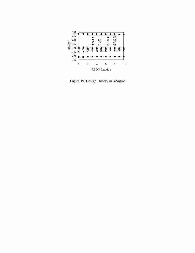
parameters, since it significantly affects uncertainty of the fatigue life [15]. Three-sigma RBDO

results of durability for the M1A1 tank roadarm are shown in Figs. 19 and 20. Note that small

design changes are made to satisfy the target fatigue life with target reliability levels, while

increasing roadarm weight 1%. The shortest fatigue life was 1.094 years at the initial design, but

increased to 5.017 years at the 3-σ optimum design. Figure 21 illustrates the fatigue life contour

of a 3-σ optimum design that has increased in overall fatigue life when compared to Figure 17.

Figure 18. Uncertainty Propagation to Fatigue Life

Figure 19. Design History in 3-Sigma


22

Figure 20. Probabilistic Constraint History in 3-Sigma

Figure 21. Fatigue Life Contour at 3-Sigma Optimum Design

4. CONCLUSIONS

This chapter presents the three key elements of an the advanced CAE methodology: durability

analysis, experimental validation, and an uncertainty-based design optimization. Since the CAE

model is developed to simulate a prototype model, the former is exposed to a variety of natural

uncertainties, which are categorized as model, physical, and statistical uncertainties. It was

proposed that a high fidelity model and analysis through experimental validation is necessary to

accurately characterize the effect of input uncertainty. Furthermore, the RBDO method must be

incorporated into CAE to take physical uncertainties into account. A lack of statistical

information in modeling physical uncertainty creates greater uncertainty that can be dealt with

using a possibility or evidence theory.

It has been found that experimental validation should be conducted to obtain a high fidelity

models and analyses. Structural durability of the Army trailer drawbar was used to demonstrate

CAE with experimental validation, and optimization was then carried out to improve the fatigue

life of the Army trailer drawbar, while minimizing its weight. To develop accurate CAE models

for multibody dynamics, FEA, and durability analysis, CAD models were carefully compared to

experimental results. Design optimization successfully increased the fatigue life of the drawbar

53.2 times and reduced the weight 40% when considering notch effects due to rivet holes in the

critical region. To validate the deterministic optimum design, a reliability analysis evaluates the


23

reliability of fatigue failure under manufacturing tolerances. The fact that its probability of

failure is 49.7% underscores the need for reliability-based design optimization (RBDO) for a

reliable and durable optimum design. In addition to experimental validation, the RBDO method

must be incorporated into advanced CAE methodology. One of challenges in developing an

advanced CAE methodology is to create an effective RBDO method. PMA was used to carry

out the RBDO process for large-scale multidisciplinary applications (e.g., M1A1 Tank roadarm

durability), with emphasis on numerical efficiency and stability. Consequently, the advanced

CAE methodology with experimental validation and uncertainty-based design optimization was

successfully demonstrated by applying it to the computationally intensive and complicated

multidisciplinary simulation process of predicting structural durability.

5. ACKNOWLEDGMENTS

Research is supported by the Physics of Failure project sponsored by U.S. Army Materiel

Systems Analysis Activity (AMSAA).

6. REFERENCES

1. Youn, B.D., Choi, K.K., and Park, Y.H., Hybrid Analysis Method for Reliability-Based Design Optimization, Journal of Mechanical Design, ASME, Vol. 125, No. 2, pp. 221-232, 2003 and Proceedings of 2001 ASME Design Engineering Technical Conferences: 27th Design Automation Conference, Pittsburgh, PA, 2001.

2. Enevoldsen, I. and Sorensen, J.D., “Reliability-Based Optimization In Structural

Engineering,” Structural Safety, Vol. 15, pp. 169-196, 1994. 3. Lee, T.W., and Kwak, B.M., “A Reliability-Based Optimal Design Using Advanced First

Order Second Moment Method,” Mech. Struct. & Mach., Vol. 15, No. 4, pp. 523-542, 1987-88.

4. Tu, J. and Choi, K.K., “A New Study on Reliability-Based Design Optimization,” Journal of

Mechanical Design, ASME, Vol. 121, No. 4, 1999, pp. 557-564.


24

5. Youn, B.D. and Choi, K.K., “Selecting Probabilistic Approaches for Reliability-Based

Design Optimization,” AIAA Journal, Vol. 42, No. 1, 2004. 6. Shih, C.J., Chi, C.C., and Hsiao, J.H., “Alternative α-level-cuts Methods for Optimum

Structural Design with Fuzzy Resources,” Computers and Structures, Vol. 81, 2003, pp. 2579-2587.

7. Bae, H.R., Grandhi, R.V., and Canfield, R.A., “Structural Design Optimization Based On

Reliability Analysis Using Evidence Theory,” SAE 03M-125, SAE World Congress, Detroit, MI, March, 2003.

8. Madsen, H.O., Krenk, S., and Lind, N.C., Methods of Structural Safety, Prentice-Hall,

Englewood Cliffs, NJ, 1986. 9. Fuchs, H.O. and Stephens, R.I., Metal Fatigue in Engineering, John Wiley & Sons, New York,

NY, 1980. 10. CADSI Inc., DADS User’s Manual, Rev. 7.5, Oakdale, IA, 1994. 11. DRAW: Durability and Reliability Analysis Workspace, Center for Computer-Aided Design,

College of Engineering, The University of Iowa, Iowa City, IA, 1994. 12. Yu, X., Choi, K.K., and Chang, K.H., “Probabilistic Structural Durability Prediction,” AIAA

Journal, Vol. 36, No. 4, pp. 628-637, 1998. 13. Haug, E.J., Choi, K.K., and Komkov, V., Design Sensitivity Analysis of Structural Systems,

Academic Press, New York, NY, 1986. 14. Arora, J.S., Introduction to Optimum Design, McGraw-Hill, New York, NY, 1989. 15. Chang, K.H., Yu, X., and Choi, K.K., “Shape Design Sensitivity Analysis and Optimization

for Structural Durability,” International Journal of Numerical Methods in Engineering, Vol. 40, pp. 1719-1743, 1997.

16. Choi, K. K., Youn, Byeng D., and Tang, Jun, “Structural Durability Design Optimization and

Its Reliability Assessment,” accepted to Proceedings of 2002 ASME Design Engineering Technical Conferences: 29th Design Automation Conference, Chicago, IL, 2003

17. Sines, G. and Waisman, J.L., Metal Fatigue, McGraw-Hill, New York, NY, 1959. 18. Youn, B.D. and Choi, K.K., “A New Response Surface Methodology for Reliability-Based

Design Optimization,” Computers and Structures, In Press, 2004.


25

19. Choi, K.K., and Youn, B.D., “An Investigation of Nonlinearity of Reliability-Based Design Optimization Approaches,” ASME Design Engineering Technical Conferences, Montreal, Canada, September 2002.

20. Youn, Byeng. D., Choi, K. K., and Yang, Ren-Jye, "Efficient Evaluation Approaches for

Probabilistic Constraints in Reliability-Based Design Optimization," 5th WCSMO, Lido di Jesolo-Venice, Italy, 2003

21. Breitung, K., Asymptotic Approximations for Multi-normal Integrals, Journal of

Engineering Mechanics, ASCE, Vol. 110, No. 3, pp. 357-366, 1984. 22. Tvedt, L., Distribution of Quadratic Forms in Normal Space-Application to Structural

Reliability, Journal of Engineering Mechanics, ASCE, Vol. 116, No. 6, pp. 1183-1197, 1990. 23. Rackwitz, R. and Fiessler, B., “Structural Reliability Under Combined Random Load

Sequences,” Computers & Structures, Vol. 9, pp. 489-494, 1978. 24. Hohenbichler, M. and Rackwitz, R., “Non-normal Dependent Vectors in Structural

Reliability,” Journal of the Engineering Mechanics, ASCE, Vol. 107, No. 6, pp. 1227-1238, 1981.

25. Wu, Y.T., Millwater, H.R., and Cruse, T.A., “Advanced Probabilistic Structural Analysis

Method for Implicit Performance Functions,” AIAA Journal, Vol. 28, No. 9, pp. 1663-1669, 1990.

26. Rusk, D.T., and Hoffman, P.C., “Component Geometry and Material Property Uncertainty

Model for Probabilistic Strain-Life Fatigue Predictions,” 6th Joint FAA/DoD/NASA Aging Aircraft Conference, San Francisco, CA, 2002.

1

Table 1. Results of Modal Analysis

Mode No. Frequency (Simulation) Frequency (Experiment) 1 18.92 17.73 2 21.55 22.14 3 26.30 29.07

2

Table 2. Design Parameters

Design Symbol Description d1 t1 Thickness of six side angles d2 t2 Thickness of two side bars d3 t3 Thickness of center bar d4 t4 Thickness of two side attachments d5 t5 Thickness of top and bottom plates d6 w Cross-section width of three bars d7 h Cross-section height of three bars

3

Table 3. Base Design and Its Bounds for Drawbar

Design Type Design dj

Lower Bound Ld

Base Design

Upper Bound Ud

d1 0.100 0.250 0.500 d2 0.100 0.250 0.500 d3 0.100 0.250 0.500 d4 0.100 0.250 0.500

Sizing Designs

d5 0.100 0.250 0.500 d6 1.000 2.000 5.000 Shape

Designs d7 1.000 3.000 5.000

4

Table 4. Critical Nodes at Base Design (Unit: Cycle)

Constraint ID Node ID Fatigue Life 1 425 9.425×106 2 424 7.148×107 3 426 1.115×1010 4 368 4.927×109 5 369 3.595×109 6 370 3.056×1010 7 4056 9.775×1011 8 4077 2.161×1011 9 4095 5.581×109 10 4099 6.137×109

5

Table 5. Design History in Optimization for HMT DRAW Durability Model

Iter Line Search W d1 d2 d3 d4 d5 d6 d7

0 58.401 0.2500 0.2500 0.2500 0.2500 0.2500 2.0000 3.00001 59.464 0.2494 0.2476 0.2762 0.2502 0.2503 1.9992 2.99662 61.186 0.2485 0.2437 0.3186 0.2506 0.2507 1.9980 2.99103 65.660 0.2462 0.2334 0.4297 0.2514 0.2519 1.9950 2.9764

1

4 60.865 0.2487 0.2444 0.3107 0.2505 0.2506 1.9982 2.99200 65.656 0.2462 0.2334 0.4297 0.2514 0.2519 1.9950 2.97641 35.712 0.1000 0.1011 0.3424 0.2283 0.2286 1.8110 2.5226

2

2 24.990 0.1000 0.1000 0.2012 0.1910 0.1910 1.5134 1.78820 35.712 0.1000 0.1011 0.3424 0.2283 0.2286 1.8110 2.52261 35.578 0.1000 0.1000 0.3417 0.2281 0.2284 1.8092 2.51832 35.473 0.1000 0.1000 0.3405 0.2278 0.2281 1.8066 2.51153 35.198 0.1000 0.1000 0.3375 0.2269 0.2272 1.7994 2.49374 34.486 0.1000 0.1000 0.3297 0.2245 0.2248 1.7804 2.4471

3

5 35.402 0.1000 0.1000 0.3405 0.2278 0.2281 1.8066 2.51150 35.198 0.1000 0.1000 0.3375 0.2269 0.2272 1.7994 2.49371 19.704 0.1000 0.1000 0.1275 0.1622 0.1623 1.2888 1.23402 24.044 0.1000 0.1000 0.1975 0.1837 0.1839 1.4590 1.65423 29.212 0.1000 0.1000 0.2676 0.2053 0.2056 1.6292 2.07404 32.190 0.1000 0.1000 0.3036 0.2164 0.2167 1.7168 2.29035 34.649 0.1000 0.1000 0.3315 0.2250 0.2253 1.7848 2.45776 34.713 0.1000 0.1000 0.3322 0.2252 0.2255 1.7864 2.4619

4

7 34.900 0.1000 0.1000 0.3369 0.2267 0.2269 1.7976 2.4896OPTIMUM 35.198 0.1000 0.1000 0.3375 0.2269 0.2272 1.7994 2.4937

6

Table 6. Constraint History in Optimization for HMT DRAW Durability Model

Iter. G1 G2 G3 G4 G5 G6 G7 G8 G9 G10 0 9.42×106 7.15×107 1.11×1010 4.93×109 3.59×109 3.06×1010 9.77×1011 2.16×1011 5.58×109 6.14×109 1 2.09×107 9.47×108 3.26×1010 2.16×1010 1.88×1010 1.28×1011 2.49×1012 4.51×1011 8.73×108 1.16×1010 2 5.90×107 2.36×109 1.06×1011 4.68×109 1.07×1011 1.46×1010 9.62×1012 4.05×1012 6.17×1010 9.99×1019 3 1.07×109 1.28×1010 2.09×1011 2.10×1012 1.13×1013 2.00×1012 2.08×1014 2.57×1013 8.48×1011 9.99×1019

1

4 5.18×107 3.37×108 4.56×1010 9.00×1010 3.67×109 4.80×1011 8.01×1012 3.38×1012 2.02×109 9.99×1019 0 1.07×109 1.28×1010 2.09×1011 2.10×1012 1.13×1013 2.00×1012 2.08×1014 2.57×1013 8.48×1011 9.99×1019 1 7.47×109 1.25×1013 2.36×109 2.00×1013 1.28×1012 9.76×109 1.62×1015 1.00×1013 9.73×1011 2.50×1011

2

2 6.00×104 1.47×109 6.60×105 5.22×108 5.10×106 1.13×109 1.05×109 6.77×108 1.27×1010 6.16×108 0 7.47×109 1.25×1013 2.36×109 2.00×1013 1.28×1012 9.76×109 1.62×1015 1.00×1013 9.73×1011 2.50×1011 1 5.08×108 6.75×1012 4.18×108 4.44×1013 3.86×1010 9.07×1011 5.79×1015 2.91×1011 1.60×1013 1.44×1011 2 2.11×1010 1.00×1013 2.70×109 3.99×1013 1.75×1011 1.07×1010 9.03×1014 7.01×1012 4.15×1010 1.97×1011 3 8.99×108 3.82×1012 1.19×109 1.12×1013 3.05×1011 1.97×109 1.78×1014 3.68×1011 7.43×1012 1.17×1011 4 2.06×108 1.74×1012 4.02×108 9.00×1012 1.64×1011 1.59×1011 4.53×1013 1.49×1012 5.34×1012 6.98×1010

3

5 4.59×108 3.67×1012 3.66×108 2.69×1013 6.23×1011 4.42×1011 1.87×1015 2.81×1012 1.69×1013 1.13×1011 0 8.99×108 3.82×1012 1.19×109 1.12×1013 3.05×1011 1.97×109 1.78×1014 3.68×1011 7.43×1012 1.17×1011 1 3.00×104 1.79×108 3.00×104 1.50×105 3.00×104 7.11×107 1.20×105 1.08×106 3.40×107 1.53×1010 2 3.00×104 1.29×109 4.20×105 4.79×108 2.55×106 8.49×108 4.08×108 3.05×108 1.69×1010 6.81×108 3 6.09×106 7.42×1010 1.10×107 9.06×1010 1.76×109 3.65×1010 2.91×1011 8.49×1010 7.88×109 1.10×1010 4 6.58×107 4.04×1011 5.56×107 3.65×1012 2.11×1010 7.27×1010 7.89×1012 6.80×1010 3.55×1012 2.02×1010 5 2.22×108 1.84×1012 4.29×108 1.23×1013 1.82×1011 1.43×1011 5.13×1013 1.57×1012 5.88×1012 7.27×1010 6 2.39×108 1.94×1012 4.48×108 7.19×1011 1.88×1011 1.54×1011 5.67×1013 1.68×1012 5.52×1012 7.60×1010

4

7 3.24×108 2.21×1012 2.47×108 8.25×1011 2.87×1011 2.22×1011 1.22×1015 6.30×1012 8.91×1012 7.30×1010 OPTIMUM 8.99×108 3.82×1012 1.19×109 1.12×1013 3.05×1011 1.97×109 1.78×1014 3.68×1011 7.46×1012 1.17×1011

7

Table 7. Design and Weight Changes between Base and Optimal Designs

Design Base Design, [in] Optimal Design, [in] Change, [%] t1 0.2500 0.1000 −60.0 t2 0.2500 0.1000 −60.0 t3 0.2500 0.3375 +35.0 t4 0.2500 0.2269 −9.24 t5 0.2500 0.2272 −9.12 h 2.0000 1.7994 −10.0 w 3.0000 2.4937 −16.9

Cost Base Design, [lb] Optimal Design, [lb] Change, [%] Weight 58.401 35.198 −39.7

8

Table 8. Fatigue Life w/o and w/ Considering Notch Effects

Predicted Fatigue Life w/o

Considering Notch Effects

w/ Considering Notch Effects

Driving Cycle, [block] 9.42×106 1.44×103 Driving Mile, [mile] 1.18×106 180 B

ase

Driving Time, [hour] 78500 12 Driving Cycle, [block] 8.99×108 7.66×104 Driving Mile, [mile] 1.12×108 9580 O

pt.

Driving Time, [hour] 7.49×106 638 Life Extension, [times] 95.4 53.2

9

Table 9. Definition of Random Parameters for Crack Initiation Fatigue Life Prediction

Parameters Lower Bound Mean Upper Bound COV Distr. type

d1, X1 1.3776 1.8776 2.0000 1 % Normal d2, X2 1.5580 3.0934 2.0000 1 % Normal d3, X3 2.5934 1.8581 3.2000 1 % Normal d4, X4 2.7091 3.0091 3.2000 1 % Normal d5, X5 2.2178 2.5178 2.7800 1 % Normal d6, X6 4.6500 2.9237 5.0000 1 % Normal d7, X7 2.6237 4.7926 3.0500 1 % Normal D

esig

n/R

ando

m

(Geo

met

ric T

oler

ance

)

d8, X8 2.5000 2.8385 3.0000 1 % Normal Fatigue Material Mean COV Distr. type

X9 Cyclic Strength Coefficient, K′ 1.358×109 3 % Lognormal X10 Cyclic Strength Exponent, n′ 0.12 3 % Lognormal X11 Fatigue Strengh Coefficient, σ′ 1.220×109 3 % Lognormal X12 Fatigue Strengh Exponent, b -0.073 3 % Normal X13 Fatigue Ductility Coefficient, ε′f 0.41 3 % Lognormal R

ando

m

(Mat

eria

l Pa

ram

eter

)

X14 Fatigue Ductility Exponent, c -0.60 3 % Normal

Figure 1. Uncertainty Types Existing in Computer-Aided Design

Model Uncertainty

Output Uncertainty

X C(X) K(X) F(X) G(X)

Simulation Model

G″(X)+C(X)G′(X)+K(X)G(X)=F(X)

Input Physical Uncertainty

Input Statistical Uncertainty

Prototype Model

Math. Model

Integrated CAE Methodology

Methods Uncertainty-Based

CAE Technology

Experimental Validations

Figure 2. Integrated Computer-Aided Engineering Methodology

Figure 3. Army Trailer and Its Structural Failure

Figure 4. CAD and Finite Element Models of Trailer

( a ) Yaw Moment of Inertia ( b ) Experimental Modal Analysis

Figure 5. Experimental Validations

Figure 6. Dynamic Model and Analysis of Trailer

( a ) Dynamic Strain ( b ) PSD Curve of Dynamic Strain

Figure 7. Validation of Dynamic Strain

Dynamic Analysis

External Forces Accelerations, and Velocities

FE Model

Quasi-static Loading

FE Analysis

Stress Influence Coeff.

Super- Position

Dynamic Stress History

Local Stress and Strain

Peak/Valley Editing

Rainflow Counting

Crack Initiation Life Prediction

Flexible Vehicle Model

Overall Vehicle Model

Figure 8. Computation Process for Fatigue Life

The Most Critical Region

Due to the Boundary Condition

Figure 9. Fatigue Life Contour of Army Trailer Drawbar

t4

t3

t2t1

t5

w

h

Figure 10. Design Parameters of Drawbar and Attachments

Stress Influence Coefficient (SIC) FE Analysis

Continuum DSA of SIC ( ) ( )' '

vm, ,u ud aδ δΩ′ψ = δ Ω + −∫ u

σ u zλ λ

Where: ( )λ is design dependant (IFGBM isthrough mass and IFED is through mass andeigenmodes). Hence eigenmodes DSA isintroduced to compute . ( )λδ

'u

Dynamic Stress History σ(t,d)

DYNAMIC PARAMETERS (ω ω ) , , , , , ra a a

Assumed no changes with small localdesign changes to improve the fatigue

Perturbed Dynamic Stress Historyσ p(t,d)= σ(t,d)+δσ

Design Perturbation δd

Perturbed Life Prediction Lp(d)=L(d)+δL

ORIGINAL LIFE PREDICTION

Fatigue Life DSA ( ) ( )( ) p

i

i i

L d LLd d

+ δ −∂=

∂ δ

d dd

Quasic-Static Loading

( ) P P T P P

r 0 0

P P p P Pd

( )

= 2

= − + ωω + ω

= − ωω + ω + ωΦ +⎧ ⎫⎪ ⎪⎨ ⎬⎪ ⎪⎩ ⎭

f r s s

f a

f

Φ Φ

m AInertia Forces due to Gross Body Motion (IFGBM)

Inertia Forces due to Elastic Deformation (IFED) mExternal & Joint Reaction Forces P

j 1.0, where s are eigenmodes=

a a

⎧ ⎫⎪ ⎪⎪ ⎪⎨ ⎬⎪ ⎪⎪ ⎪⎩ ⎭Φ

Figure 11. Design Sensitivity Computational Procedure for Flexible Structural Systems

369370

36840954077

( a ) Life Contour on Top of Drawbar at Base Design

425

4056 424

4099

426

( b ) Life Contour on Bottom of Drawbar at Base Design

Figure 12. Fatigue Life Contour on Drawbar at Base Design

425

4244056

4099

( a ) Life Contour on Top of Drawbar at Optimal Design

369370

3684095

4077

426

( b ) Life Contour on Bottom of Drawbar at Optimal Design

Figure 13. Fatigue Life Contour on Drawbar at Optimal Design

Failure Surface g2(X)=0

0

Failure Surface g1(X)=0

Infeasible Region, gi(X)>0

RBDO Optimum Design w/ Desired Reliability

Deterministic Optimum Design – 50% Reliability

Joint PDFfX(x) Contour

Feasible Region, gi(X)≤0 X2

X1

Initial Design

Figure 14. Overall Procedure of PMA+ in RBDO

Roadarm

Figure 15. Military Tracked Vehicle

x1

x2

x3

Torsion

Center of the Roadwheel

Intersection 3 d5, d6 Intersection 4

d7, d8

Intersection 1 d1, d2 Intersection 2

d3, d4

Figure 16. Random Design Parameters

Low fatigue Region Figure 17. Preliminary Fatigue Life Analysis

0.00

0.10

0.20

0.30

0.40

0.50

1.0E+05 1.0E+06 1.0E+07 1.0E+08

Fatigue Life [cycle]

Pro

babi

lity

of F

ailu

re PDF1 (Geo)PDF2 (Geo+Mat)

±3σLife2

±3σLife1

Figure 18. Uncertainty Propagation to Fatigue Life

1.52.02.53.03.54.04.55.0

0 2 4 6 8 10

RBDO IterationD

esig

n

d1 d2d3 d4d5 d6d7 d8

Figure 19. Design History in 3-Sigma

-5.0

-4.0

-3.0

-2.0

-1.0

0.0

1.0

0 2 4 6 8 10

RBDO IterationPr

obab

ilisti

c G

Gp1 Gp2Gp3 Gp4Gp5 Gp6

Figure 20. Probabilistic Constraint History in 3-Sigma

Date post:	26-May-2018
Category:	Documents
Upload:	dangduong
View:	216 times
Download:	0 times

UNCERTAINTIES AND MULTIDISCIPLINARY …user.engineering.uiowa.edu/~kkchoi/D_RBDO_B.06.pdf · ·...

Documents