THESIS FOR THE DEGREE OF DOCTOR OF PHILOSOPHY Uncertainty and sensitivity analysis applied to LWR neutronic and thermal-hydraulic calculations AUGUSTO HERNÁNDEZ-SOLÍS Division of Nuclear Chemistry Department of Chemical and Biological Engineering CHALMERS UNIVERSITY OF TECHNOLOGY SE‐412 96 Göteborg, Sweden 2012
Transcript
THESIS FOR THE DEGREE OF DOCTOR OF PHILOSOPHY
Uncertainty and sensitivity analysis applied to
LWR neutronic and thermal-hydraulic calculations
AUGUSTO HERNÁNDEZ-SOLÍS
Division of Nuclear Chemistry
Department of Chemical and Biological Engineering
CHALMERS UNIVERSITY OF TECHNOLOGY
SE‐412 96 Göteborg, Sweden 2012
Uncertainty and sensitivity analysis applied to LWR neutronic and thermal-hydraulic calculations AUGUSTO HERNÁNDEZ-SOLÍS ISBN 978-91-7385-734-5
Doktorsavhandlingar vid Chalmers Tekniska Högskola Ny serie nr 3415 ISSN 0346-718X
Nuclear Chemistry Department of Chemical and Biological Engineering Chalmers University of Technology SE-412 96 Göteborg Sweden Telephone +46 (0) 31-772 1000 Cover: Illustration of the uncertainty analysis performed on nodal core calculations of LWRs Chalmers Reproservice Göteborg, Sweden 2012
Uncertainty and sensitivity analysis applied to LWR neutronic and thermal‐hydraulic calculations
AUGUSTO HERNÁNDEZ‐SOLÍS Division of Nuclear Chemistry
Department of Chemical and Biological Engineering
Chalmers University of Technology
ABSTRACT
Nowadays, with an increased number of light water reactors (LWRs) around the world, there is a large interest
in improving deterministic safety analysis as an essential tool for demonstrating the safety of nuclear power
plants. Best estimate (BE) computer codes were developed to model the complex and strong coupling that
exists between the neutron and thermal‐hydraulic fields that are present in the core of nuclear reactors. At
present, these are employed (among other applications) in the prediction of the safety margins of nuclear
power plants during normal and off‐normal operating conditions. Nevertheless, even if the best available
science is applied in the modeling of nuclear reactors, uncertainties are always present in the calculations. In
recent years, it has been recognized by the nuclear community that if useful conclusions are to be obtained
from BE codes, these should be supplemented by a quantitative uncertainty analysis. In this thesis, uncertainty
and sensitivity analysis is performed on neutronic and thermal‐hydraulic calculations of LWRs. A statistical
approach is employed, where the non‐deterministic treatment of a physical model that induces a stochastic
nature on the code outputs is based on a sampling methodology. The preferred sampling strategy for the
current study corresponds to the quasi‐random Latin Hypercube Sampling (LHS). This technique allows a much
better coverage of the input uncertainties than simple random sampling (SRS) because it densely stratifies
across the range of each input probability distribution. This is one of the first works that employs LHS to sample
the input uncertain space, and then relies on the concept of non‐parametric tolerance intervals for the code
output uncertainty assessment for both neutronic and thermal‐hydraulic calculations. It is shown at the
different stages in the modeling of LWRs that LHS offers the possibility to assess more realistic non‐parametric
tolerance limits than SRS, because code non‐linearities are much better handled when the input space is
covered in an efficient way.
The deterministic modeling of LWRs begins with the computation of energy‐collapsed and homogenized
macroscopic cross‐sections by means of a lattice code. Once these parameters are functionalized as a function
of the reactor state variables and discretized in space, they are used as input variables by core simulators in
order to calculate the spatial distribution of the neutron flux and thus, the spatial distribution of the power.
Once the power is determined, the thermal‐hydraulic variables are updated, and the process repeated until
convergence. This thesis is divided in three different parts related to the possible neutronic and thermal‐
hydraulic modeling strategies. In the first part, microscopic cross‐section uncertainties based on two modern
nuclear data libraries such as JENDL‐4 and ENDF/B‐VII.1 were derived in multi‐group format. These were
propagated through lattice calculations in order to perform uncertainty analysis on the infinite neutron
multiplication factor ( , and on two‐group homogenized macroscopic cross‐sections corresponding to a PWR
fuel segment. The aim is to compare the uncertainty assessment on and on the macroscopic cross‐sections
when the different nuclear libraries are employed. It was found that the computed uncertainties based on
JENDL‐4 are much higher than the computed uncertainties based on ENDF/B‐VII.1. A sensitivity analysis
showed that the multi‐group variances of the Uranium‐235 fission reaction based on JENDL‐4 are very high,
being this the main reason of the observed large discrepancies in the different uncertainty assessments.
In the second part of the thesis, two types of uncertainty analyses were performed on core simulations. The
first one corresponds to the forward approach of input uncertainty propagation, where the input uncertain
space formed by the nodal two‐group macroscopic cross sections and diffusion coefficients is sampled both
with SRS and LHS. The possible ranges of variation of such an input space are based on data from a depletion
calculation corresponding to the cycle 26 of the Swedish Ringhals‐1 BWR. The aim of this study is to compare
the efficiency of the uncertainty assessment performed on the nodal thermal flux when SRS and LHS are
employed. On the other hand, in the second type of uncertainty analysis presented in this chapter,
discrepancies between spatial measured and calculated fluxes in Ringhals‐1 are used to perform an inverse
uncertainty analysis on the spatial dependence of the different core parameters. This analysis is carried out
using Bayesian statistics, where, for a certain cycle, the frequency distributions of macroscopic cross‐sections
and diffusion coefficients at every assembly node are updated based on the error distribution of the spatial
thermal flux. Emphasis was made on performing uncertainty analysis as well on the coefficients of a nodal
cross‐section model. Although a very simple model was derived, the aim is to propose an uncertainty
assessment based on replicated sampling techniques such as the general bootstrap method.
Finally, in the third part of the thesis, uncertainty and sensitivity analyses were applied to thermal‐hydraulic
calculations. The objective is to show that when experimental data are available, uncertainty analysis can be
used in the validation process of a BE code. Quantitative limits based on a statistical theory were computed to
validate code thermal‐hydraulic features in predicting pressure drop, void fraction and critical heat flux based
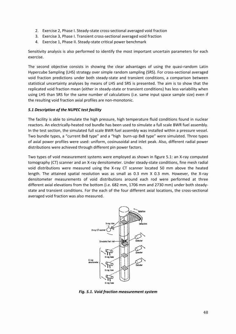
on the macroscopic exercises of the OECD/NRC BWR Full‐Size Fine‐Mesh Bundle Test (BFBT) benchmark.
The present study performs a realistic analysis of nuclear reactors, particularly in the uncertainty prediction of
important neutronic and thermal‐hydraulic parameters of light water reactors.
Keywords: Nuclear best estimate codes, uncertainty analysis, sensitivity analysis, Latin Hypercube Sampling,
simple random sampling.
Puedes llamarmeCuauhtecuhtli, el Señorde lasÁguilas.He venidoa llevartea tulugar en el centro de las Cuatro Sendas; por tu valentía y honor has ganado laentradaenlosCuacuahtzin,losCaballerosÁguila…
LIST OF PUBLICATIONS
This thesis is based on the work contained in the following papers:
PAPER I
Hernández‐Solís A., Demazière C., Ekberg C. “Uncertainty and sensitivity analyses applied to the
DRAGONv4.05 code lattice calculations and based on JENDL‐4 data”
Submitted to Annals of Nuclear Energy
PAPER II
Hernández‐Solís A., Demazière C., Ekberg C. “Uncertainty analyses applied to the UAM/TMI‐I lattice
calculations using the DRAGONv4.05 code and based on JENDL‐4 and ENDF/B‐VII.1 covariance data”
Submitted to Science and Technology of Nuclear Installations
PAPER III
Hernández‐Solís A., Demazière C., Ekberg C. “Bayesian uncertainty analysis of BWR core parameters
based on flux measurements”
ANS Winter Meeting Transactions, Vol. 105, 2011.
PAPER IV
Hernández‐Solís A., Ekberg C., Demazière C. “Uncertainty analysis of a nodal cross‐section model
based on Ringhals 1 data by means of a non‐parametric bootstrap method”
Submitted to Progress in Nuclear Energy
PAPER V
Hernández‐Solís A., Ekberg C., Ödegård‐Jensen A., Demazière C., Bredolt U. ”Statistical uncertainty
analyses of void fraction predictions using two different sampling strategies: Latin Hypercube and
random sampling”
18th International Conference on Nuclear Engineering (ICONE), 30096, 2011.
PAPER VI
Hernández‐Solís A., Ekberg C., Demazière C., Ödegard‐Jensen A., Bredolt U. “Uncertainty and
sensitivity analyses as a validation tool for BWR bundle thermal‐hydraulic predictions”
Nuclear Engineering and Design, Vol. 241 (9), 2011.
LIST OF PUBLICATIONS NOT INCLUDED IN THIS THESIS
Pazsit I., Demazière C., Sunde C., Bernitt P., Hernandez-Solis A. “Final Report on the Research
project Ringhals Diagnostics and Monitoring Stage 12”. CTH-NT-220/RR-14, August 2008.
Hernández‐Solís A., Vinai P., Bredolt U. “An assessment study of the POLCA‐T code bases on NUPEC
data”. ANS Annual Meeting Transactions, Vol. 100, 2009.
Hernández‐Solís A. “Uncertainty and sensitivity analysis applied to the validation of BWR bundle
thermal‐hydraulic calculations”. Licentiate thesis, CTH‐NT‐231, Chalmers University of Technology,
2010.
Hernández‐Solís A., Carlsson F. “Diagnosis of submersible centrifugal pumps: A motor current and
power signature approach”. European Power Electronics and Drives Journal, Vol. 20 (1), 2010.
Pazsit I., Montalvo C., Hernández‐Solís A., Bernittt‐Cartemo P., Nylen H. “Diagnostics of core barrel
and fuel assembly vibrations in the Swedish Ringhals PWRs”. 7th International Topical Meeting on
Nuclear Plant Instrumentation, Control, and Human‐Machine Interface Technologies 2010, NPIC and
HMIT 2010, Las Vegas, NV, USA.
Hernández‐Solís A., Demazière C., Ekberg C., Ödegaard–Jensen A. “Statistical uncertainty analysis
applied to the DRAGONv4 code lattice calculations and based on JENDL‐4 covariance data”. On the
proceedings of PHYSOR 2012‐Advances in Reactor Physics, Knoxville TN, USA.
Hernández‐Solís A., Demazière C., Ekberg C. “Statistical uncertainty analysis applied to the neutron
flux predictions of a BWR core using two different sampling strategies: Latin Hypercube and random
“A nuclear power plant is infinitely safer than eating, because
300 people choke to death on food every year”
James Allen
1.1 Background
At the end of the year 2011, nuclear energy provided about 15% of the world’s electricity as a
continuous and reliable based‐load power. Nowadays, nuclear energy is experiencing a renaissance
because it represents a very good option to fulfill the growing demand for electricity around the
globe. Concerns over climate change and dependence on unsecure supplies of fossil fuels are the
main reasons for such a renaissance. According to a 2012 joint study between the OECD Nuclear
Energy Agency (NEA) and the International Atomic Energy Agency (IAEA) [1], although the Fukushima
Daiichi nuclear accident has affected nuclear power policies and projects in some countries, nuclear
power remains a key part of the global energy mix. Several governments have plans for constructing
new nuclear plants, with the strongest expansion expected in China, India, Republic of Korea and the
Russian Federation. Therefore, with an increased number of light water reactors (LWRs) in the
world, there is a huge interest in improving deterministic safety analysis as an essential tool for
demonstrating the safety of nuclear power plants. The main objective of safety analysis is to
demonstrate in a robust way that all safety requirements are met; that is, that sufficient margins
exist between the real values of important parameters (e.g. peak cladding temperature) and the
threshold values at which the barriers against release of radioactivity would fail [2].
The strong coupling between the neutron kinetics and thermal‐hydraulics is a unique feature of
LWRs, which makes the calculation of their behavior a very challenging task. The so‐called nuclear
best estimate (BE) codes are complex tools developed to predict how the neutron density field (i.e.
the spatial and temporal distribution of the neutron density throughout the core) interacts with the
density field of the coolant and the temperature field of the fuel (i.e. the spatial and temporal
distribution of the enthalpy of the coolant/temperature of the fuel throughout the core). The
common modeling strategies all rely on separate modeling tools for resolving the different fields and
possibly the different scales. The interdependence between the different fields/scales is usually
accounted for by software coupling. Nuclear codes are used nowadays not only to estimate the
transient behavior of light water nuclear power plants during off‐normal conditions, but also for the
evaluation of safety margins. The training of operators, the optimization of the plant design and
related emergency operating procedures are some of the applications of such codes. Nevertheless,
even though modern nuclear codes are based on the best available science, uncertainties are always
present in the calculations. They originate from different sources like for instance, a lack of
knowledge in the physical interpretation and representation of the code models, as well as plant and
fuel parameters that are input data for the code. Therefore, it has been recognized by the nuclear
community that if useful conclusions are to be obtained from BE calculations, these should be
supplemented by a quantitative uncertainty analysis. On the other hand, the study of how output
uncertainty can be apportioned to the different input sources, known as sensitivity analysis, is an
important complement to uncertainty quantification since it identifies the parameters where a
2
reduction of the uncertainty will have the greatest benefit for the reduction of the total simulation
uncertainty.
Prior to having the capability to calculate the uncertainty of key values that define a nuclear power
plant operational limits, conservative calculations of the safety margins were performed during the
1970s. For example, in the United States, prior to the existence of Appendix K to Title 10 Part 50 of
the Code of Federal Regulations (10 CFR 50) [3], regulatory bodies required that all calculations of the
limiting parameters should be performed using specified conservative procedures. In 1988, the 10
CFR 50.46 amendment allowed the use of BE codes for performing safety analysis, stipulating that
uncertainties must be identified and quantified. At present, in the existing International Atomic
Energy Agency (IAEA) safety standards [4], the use of BE codes with realistic input data plus
uncertainty analysis is recognized as an acceptable option for demonstrating that safety is ensured
with an adequate margin. This constitutes the backbone of state‐of‐the art international licensing
regulations. The modern concept of safety margin is presented in figure 1.1.
Fig. 1.1. Concept of safety margin given by the IAEA [3]
1.2 Objectives
In this thesis, uncertainty analysis is performed at different neutronic and thermal‐hydraulic LWR
modeling stages using a Monte Carlo‐based approach, where the non‐deterministic treatment of a
physical model that induces a stochastic nature on the code outputs is based on a sampling
methodology. In this approach, the code input space defined by input parameters, boundary and
initial conditions, sub‐models, etc. are treated as random variables. Thereafter, values of these inputs
are selected according to a random or quasi‐random sampling strategy and then propagated through
the code in order to assess the output uncertainty in the corresponding calculations. This framework
has been highly accepted by many scientific disciplines not only because of its solid statistical
foundations, but also because it is affordable in practice and relatively easy to implement thanks to
the tremendous advances in computing capabilities.
The preferred sampling strategy for the current study corresponds to the quasi‐random Latin
Hypercube Sampling (LHS). This technique allows a much better coverage of the input uncertainties
than simple random sampling (SRS) because it densely stratifies across the range of each input
probability distribution. In fact, LHS was born in the field of safety analysis of nuclear reactors [5],
and one of the goals of this work is to prove the benefits and efficiency of using LHS over SRS in both
LWRs neutronic and thermal‐hydraulic predictions. Once a sample of the code output has been
taken, a statistical inference of the output population parameters is performed. During recent years,
it has been common in the field of nuclear reactor safety to use the theory of non‐parametric
3
tolerance limits for the assessment of code output uncertainty. This approach is based on the
minimum sample size required to infer a certain coverage of a population, with a certain confidence.
Thus, the different code output uncertainty assessments performed in this work along the neutronic
and thermal‐hydraulic calculations are based on the concept of non‐parametric tolerance limits. In
this thesis, emphasis is made in the computation of multivariate tolerance limits when the code
output space is comprised by several parameters that are correlated, because the statistical coverage
of the output space depends on the number of correlated parameters. The fact that this statistical
theory is solely based on the ranking of the output space sample, makes it possible to use it even if
the input space has been sampled with LHS or any kind of stratification, and not only with SRS. This is
explained in much more detail in the next chapter.
All in all, the main objective of the thesis was to perform an uncertainty analysis at all possible stages
in the deterministic neutronic and thermal‐hydraulic modeling of LWRs, in order to have a
quantitative measurement of the uncertainties that are associated to the different parameters that
are used to study the physical behavior of light water reactors.
1.3. Outline of the thesis
This thesis begins with a review of the statistical approach to perform uncertainty analysis, where
LHS and SRS are explain in detail. The following chapters are related to the three main stages that are
currently employed in the modeling of the neutronic and thermal‐hydraulic fields of the core of
LWRs. In chapter 3, microscopic cross‐section covariance data in multi‐group form was derived from
modern nuclear data libraries. The different covariance matrices were propagated through the
DRAGONv4.05 lattice code, in order to assess a degree of uncertainty to the energy‐collapsed and
homogeneized macroscopic cross‐sections and diffusion coefficients. Thus, a comparison between
the computed uncertainties based on JENDL‐4 and ENDF/B‐VII.1 data was performed on a 15x15
PWR fuel segment test case corresponding to the Exercise I‐2 of the OECD/NEA UAM benchmark.
Also, a brute sensitivity analysis is made on a 17x17 PWR case based on JENDL‐4 data, in order to
know which microscopic cross‐section has the biggest influence on the infinite neutron multiplication
factor.
Chapter 4 deals with a forward and inverse uncertainty analysis performed by core calculations. The
forward analysis aims to prove that LHS is much more computational efficient than SRS in the
computation of the maximum achievable uncertainty of the nodal thermal flux. On the other hand,
the inverse study aims to obtain posterior PDFs of nodal macroscopic cross‐sections and diffusion
coefficients using a Bayesian uncertainty analysis. This is based on the discrepancies between spatial
measured and calculated fluxes that were used in the fuel loading strategy of the Ringahls 1 BWR
during cycle 26. Therefore, the goal is to obtain uncertainty ranges of the nodal core parameters that
rely on experimental data.
In chapter 5, uncertainty and sensitivity analyses were performed to steady‐state and transient void
fraction predictions. One of the main objectives is to enhance the validation process of the thermal‐
hydraulic features of the Westinghouse code POLCA‐T. This is achieved by computing a quantitative
validation limit based on statistical uncertainty analysis. Finally, some general conclusions about this
work are given in chapter 6, as well as some reflections about what can be done in the future in the
field of uncertainty analysis applied to nuclear reactors simulations.
4
5
CHAPTER 2
PROPAGATION OF UNCERTAINTY IN THE ANALYSIS OF NUCLEAR
SYSTEMS
“Statistics are like bikinis. What they reveal is suggestive, but what they conceal is vital”
Aaron Levenstein
One of the main parts of the uncertainty analysis consists in the identification and characterization of
the relevant sources of uncertainty, which define the so called “input uncertainty space”. Some
authors have classified the different sources under five general categories [6,7]. A few neutronic and
thermal‐hydraulic examples of each category are given in table 2.1.
Table 2.1. Different sources of uncertainty that are commonly present in LWR calculations
Neutronic Thermal‐hydraulic
Code or model uncertainty
Approximations on the angle dependence of the neutron flux (i.e. only taking into consideration up to the P1 component), or the use of diffusion theory in the prediction of the nodal neutron flux in the reactor core.
Including only some terms in the field equations (e.g. the viscous stress terms are sometimes not included), uncertainties in constitutive correlations, assuming that fully developed flow exists in the system are only a few examples included in this group.
Representation uncertainties
The chosen numerical method to discretize the neutron flux spatial dependence.
The chosen nodalization of the system that define the control volumes where the field equations are going to be solved.
Scaling uncertainties
Using data recorded in scaled experimentsand the reliance on scaling laws if applicable, constitute a source of uncertainty.
Plant uncertainty
Neutron cross‐sections were obtained mainly from experiments. Nowadays, the trend is to simulate the possible probabilities of neutron interactions with matter.
Boundary and initial conditions of the nuclear power plant into consideration are uncertain because in many cases they come from measurements. Other system components parameters such as the time when a pump or valve is tripped, controller parameters, etc., are also considered here.
User effect It has been recognized that the degree of user expertise and experience in handling complex BE codes, can add uncertainty to the desired results. It should be acknowledged at the beginning of any input deck design that this type of uncertainty exists, so the user can take the necessary actions to reduce this effect.
Generally speaking, sources of uncertainty can arise from two different broad categories. First, there
is the uncertainty that arises because the system under study can behave in many different ways.
This type of uncertainty is often referred to as stochastic or aleatory uncertainty, and is a property of
the system under consideration due to random or inherent variation [8]. This uncertainty is
irreducible and includes the basic statistical concepts of variability and the definition of probability as
describing the uncertainty associated with the outcome of an experiment or event. An example of
this type of uncertainty is, for instance, the time when a pump is tripped during a power plant
transient. Second, there is the uncertainty that arises from an inability to specify the exact value of a
6
quantity that is assumed to have a constant value within a particular analysis. This type of
uncertainty is often referred to as subjective or epistemic uncertainty [8]. By contrast to the aleatory
uncertainty, epistemic uncertainty is reducible and stems from a lack of knowledge. The other main
part of the uncertainty analysis characterizes the methodology to quantify the global influence of the
combination of the input uncertainties on selected output parameters, which now define the so
called “output uncertainty space”. It can be said that the two main items of uncertainty analysis may
be treated differently by different methodologies.
Within the most important methodologies applied in the reactor safety analysis field, uncertainties
are evaluated using two approaches: a) Propagation of input uncertainties or b) Extrapolation of
output uncertainties. In the first approach, uncertain input parameters are characterized by specific
ranges and/or probability density functions (PDFs), and calculations are performed varying such
parameters. Deterministic and statistical methodologies follow this approach. However, in the
extrapolation of output uncertainty approach, the output uncertainty is based on comparisons
between calculation results and significant experimental data. These two approaches are illustrated
in figure 2.1.
Fig. 2.1. Uncertainty classification. a) Propagation of input uncertainty; b) Propagation of output uncertainties [3]
In this chapter, sampling‐based methods that are employed for performing uncertainty and
sensitivity analysis are presented, since the work of this thesis is based on this approach. A literature
review of other uncertainty methodologies that are used in the safety analysis of nuclear reactors
7
such as the deterministic adjoint sensitivity analysis procedure (ASAP), or the one belonging to the
propagation of output uncertainties approach, such as the uncertainty methodology based on
accuracy extrapolation (UMAE), was made at the beginning of the present PhD project and can be
found in the corresponding Licentiate thesis [9].
2.1 Overview of the statistical methodology
The non deterministic treatment of a physical model that induces a stochastic nature on the result
can be studied with statistical methods. The first step of this framework is to identify the most
important uncertain parameters defined as , , … , . They should be characterized by a
sequence of probability density functions (PDFs) , , … , , defining the uncertain input space.
Then, a sampling strategy is used to generate a sample of size N from such input space which is
propagated through the code in order to treat the output calculations , , … , as random
variables. This scheme is shown in figure 2.2.
Fig. 2.2. Scheme of statistical uncertainty analysis [10]
The definition of the PDFs is one of the most important parts of the statistical methodology because
these distributions determine both the size and the distribution of the uncertainty in the model
results. Nevertheless, their characterizations have been widely based on formal expert review
processes. In this case, the investigator decides the plausible range of variation for each input. A
small range usually maintains numerical stability of the code meanwhile a large range will lead to
more useful information about the code behavior. However, the choice is made by intuition or
guesses and might have to be revised after some model runs [11,12]. The next step is to assign
probability distributions to characterize a degree of belief with respect to where the appropriate
value of each element is located. Unfortunately, contrary to the aleatory uncertainty where
observational and/or experimental results might help to find out a probability distribution, data will
often not be available to characterize epistemic uncertainty, thus making the distribution assignment
somewhat arbitrary. Common choices for distributions are the uniform, normal and lognormal for
continuous variables. For discrete variables probability functions like the binomial or Poisson
distributions can be used.
The care and effort used in the definition of the distributions are dependent on both the purpose of
an analysis and the amount of time and resources available for its implementation. It is expected that
experts could offer assistance in understanding and estimating uncertainties in the modeling process
without contributing to additional uncertainty. However, an analyst’s decision can contribute to the
overall uncertainties in the modeling process from the cognitive biases that affect subjective
judgment. Some authors [13] have expressed their concern about how the so‐called expert opinion
underestimates uncertainty quantification. Other human facts that may affect uncertainty
assessment are:
8
Availability. How analysts account for certain events depends upon whether they have
experienced them or not.
Misimpression. Poor, incorrect or bad translation of information.
Anchoring. Some analysts tend to anchor to preconceptions even in light of new data or
information.
During the last years, the effort to generate relevant experimental data designed to study important
phenomena such as separate effect tests, have raised the question whether expert opinion should be
replaced by a quantitative uncertainty assessment based on the difference between code and
experimental agreements. For instance, the Canadian regulatory body agrees on the BE plus
uncertainty approach for licensing purposes if input uncertainties are assessed against relevant
experiments [2]. Signal processing techniques based on Bayesian statistics in order to quantify a
posteriori distributions based on experiments, is a good example of such a type of assessment [14].
2.1.1 Sampling strategies
The statistical methodology relies on a sampling strategy in order to propagate input uncertainties
through the code. The simplest sampling procedure for developing a mapping from analysis inputs to
analysis results is random sampling. In this procedure, each sample element is generated
independently of all other sample elements; however, there is no assurance that a sample element
will be generated from any particular subset of the input space. In particular, important subsets with
low probability but high consequences are likely to be missed if the sample is not large enough.
Furthermore, if sampled values fall closely together, the sampling is quite inefficient. In order to
overcome this issue, the stratified‐based Latin hypercube sampling was derived.
A brief but good historical review of the Latin Hypercube development is made by Helton et al. in [5].
LHS has its origins in the reactor safety community during the mid 1970’s, when the treatment of
uncertainty in analyses related to the safety of NPP started being a big concern, leading to an active
interest from the US Nuclear Regulatory Commission (NRC) and its contractors in the propagation of
uncertainty through models of complex systems. LHS is done according to the following scheme to
generate a sample of size from the input space in consistency with their PDFs. The range of each
variable (i.e. the ) is exhaustively divided into disjoint intervals of equal probability and one value
is selected at random from each interval. The values thus obtained for are paired at random
without replacement with the values obtained for . These pairs are combined in a random
manner without replacement with the values of to form triples. This process is continued
until a set of is formed. In this way, a good coverage of all the subsets defining the
uncertain input space can be achieved. Therefore, LHS can be viewed as a compromise, since it is a
procedure that incorporates many of the desirable features of random and stratified sampling. The
LHS procedure is exemplified in figure 2.3 for two different possible input distributions, one
corresponding to a uniform distribution and the second to a normal distribution, respectively.
9
Fig. 2.3. Coverage of a probability space formed by a uniform and normal distributions using LHS
and for a sample size of 10 elements
If the coverage performed with LHS is to be compared to the SRS case, it is straightforward to see
that LHS will perform better or at least equivalently in covering the joint range of the PDFs depending
on the type, number of distributions forming the space and desired number of samples. For instance,
in figure 2.4, the samples of 10 elements obtained from the previous two distributions are paired
using both LHS and SRS, so a comparison of the coverage computed by the two sampling techniques
can be made.
Fig. 2.4. Performance of LHS vs. SRS in covering with 10 samples the space formed by a uniform and
normal PDFs
It can be seen from the pairing of the different samples that for the SRS case, parts of the space
where not even covered, while in the LHS case for every row and column there is at least one point
being sampled. Thus, for the same sample size, LHS covered much better the input space than SRS.
It is of interest to study the properties of the different sampling techniques used for estimating the
mean, variance and confidence depending on the range of variation of a particular output variable
from code predictions defined as , 1, … , . McKay et al. [15] established that if is
monotonic in each of the , then the variance of the estimated output mean using LHS would be less
than or equal to the variance of the estimated output mean using SRS, i.e.:
2.1
10
Where:
1⁄ 2.2
For each sampling method, the form for the estimator of the output variance is given by:
1 1⁄ 2.3
When using the SRS procedure, it is well known that Eq. (2.3) is an unbiased estimator of the output
variance, i.e. . However, if LHS is employed, is an asymptotically biased
estimator. McKay et al. [15] also proved that, if is monotonic in each of the , the expected value
of the LHS variance estimator varies between:
1
2.4
Even if was found to have a little bias, it was also found to have less sampling variability than
. This result, together with Eq. (2.1), suggests that the 1 confidence interval of the
predicted output mean is smaller for the LHS strategy than for the SRS one, considering that both
have the same sample size . Such confidence interval can be computed as:
√
2.5
Where corresponds to the 1 2⁄ quantile of the t‐distribution with 1 degrees of
freedom.
Thus, the uncertainty analysis is more efficient with LHS not only for presenting less sampling
variability on the estimation of the output parameters, but also due to the fact that it can much
better handle the code non‐linearities. The reason lies with a much better coverage of important
regions of the input space than SRS, if the sample size is the same.
The LHS methodology previously described assumes that the different variables are independent.
Nevertheless, Iman and Conover [16] developed a Latin hypercube procedure developed for
sampling correlated variables. Such procedure is based not directly on the covariance matrix but
instead, on the correlation matrix (which should be positive definite).
The procedure begins by taking an LHS sample based on the individual variances, and assuming that
the input parameters are independent, e.g.:
⋯⋯
⋮ ⋮ ⋮ ⋮⋯
2.6
Where m is the total number of inputs, and n the number of samples. The aim of this procedure is to
rearrange the values in the individual columns of , so that a desired rank correlation structure
results among the individual variables. This can be achieved by somehow relating the correlation
coefficients of the matrix, to the total correlation matrix .
11
If the correlation matrix of is called , the method applies a Cholesky decomposition to both
and in order to obtain, respectively, the and lower triangular matrices that satisfy the
following relationships:
(2.7)
Then, the target or desired matrix ∗ can be computed such as:
∗ 2.8
Where the matrix relates and as follows:
2.9
In the end, ∗ has a correlation matrix equal to , and the values of each variable in must be
rearrange so that they have the same rank (order) as the target matrix ∗. That is why this method is
known as the rank‐induced method.
2.2 Uncertainty assessment using non‐parametric tolerance limits
Once a sample of the code output has been taken, a statistical inference of the output population
parameters is performed. During recent years, it has been common in the field of nuclear reactor
safety to use the theory of non‐parametric tolerance limits for the assessment of code output
uncertainty. This approach, proposed by Gesellschaft für Anlagen‐ und Reaktorsicherheit (GRS) [17],
is based on the work done by Wilks [18,19] to obtain the minimum sample size in order to infer a
certain coverage of a population, with a certain confidence. One first assumes that the uncertainty
assessment is only performed in one output parameter. For the one‐sided tolerance limit case,
where 100 (%) represents the confidence level that the maximum code result will not be
exceeded with an 100 (%) probability, the required sample size n is given by [20]:
1 2.10
This means that once the output sample is ranked, the maximum value of the sample infers the
100 percentile of the output population with a 100 % of confidence. For example, for an
estimation of the 95th percentile with a 95% of confidence a sample of 59 elements is required.
For the two‐sided case, where the coverage of the output population is expected to be inferred from
the 100 100 percentile to the 100 percentile with a 100 % of confidence,
the minimum sample size is given by the following implicit equation [20]:
1 1 2.11
For example, if the 5th and 95th percentiles of the population are to be inferred with a 95% of
confidence, a sample size of 93 elements is required. It should be noticed that this analysis is solely
based on the number of samples and applies to any kind of PDF the output may follow. Also, since
the input space is only used as an indirect way to sample the output space, the use of non‐
parametric tolerance limits is independent from the number of uncertain input parameters. When
12
the code output is comprised by several variables that depend on each other, the uncertainty
assessment should be based on the theory of multivariate tolerance limits. Wald [21,22] was the first
to analyze the statistical coverage of a joint distribution‐free PDF. In Guba et. al. [23], the concern
about assessing separate tolerance limits to statistically dependent outputs was raised within the
nuclear reactor safety community. In this work, it was shown that the general equation developed by
Noether [24] for simultaneous upper and lower tolerance limits can be used to determine the
minimum sample size required to cover, in a distribution‐free manner, a joint PDF depending on the
number of output variables. Such equation reads as follows:
1 1 2.12
Where r is related to the number of upper tolerance limits and m is related to the number of lower
tolerance limits to be assessed. For instance, in the case of two‐sided tolerance limits for a single
variable, 1 and Eq. (2.12) turns out to be the same as Eq. (2.11). On the other hand, for the
case of one‐sided tolerance limit (i.e. upper limit) of a single variable, 1 and 0 and Eq. (2.12) will be the same as Eq. (2.10). Therefore, if a two‐sided uncertainty assessment is going to be
performed to 2 statistically dependent output variables then 2, and so on. It should be noticed that the sample size in the multivariate case depends on the correlation among the different
parameters. Guba et. al. [23] exemplified this fact for a bivariate normal distribution. It was then
shown that if the variables were highly correlated, the required sample size to cover the joint PDF is
smaller than for the poorly correlated case. Nevertheless, if nothing is known about the output space
PDF, Eq. (2.12) would give the required sample size for the desired multivariate coverage with a
desired confidence independently of the correlation (or covariance) among the output parameters.
This is a very powerful statistically significant way to assess uncertainty in the design of
computational experiments since in general, nothing is known about the PDF from which the
calculations are coming from.
Other authors have done some work deriving the minimum sample size for multivariate non‐
parametric tolerance limits, such as the equation presented by Scheffé et. al. [25]:
,2 1 1
1 2.13
Where , is the value of the ‐distribution with 2 degrees of freedom. Ackermann
et. al. [26] tabulated Eq. (2.13) as a function of the desired coverage and confidence, respectively, for
a large number of tolerance limits the space in study may be comprised with. These tables are in
agreement with for instance, table No. 4 shown in [23] with respect to the solution of Eq. (2.12) for
the two‐sided case and up to 3 variables in question.
2.3 LHS and the uncertainty assessment based on non‐parametric tolerance limits
Michael McKay, one of the creators of LHS, stated in reference [27] that there are no exact methods
for constructing tolerance intervals for an output using LHS. It is claimed there that the output values
from an LHS do not constitute a random sample from its distribution. Nevertheless, other authors
[5,28] have suggested that the use of LHS applied to the inference of code output tolerance limits in
a non‐parametric way is valid. In this thesis, these are the following reasons why it is believed that
LHS can be used to estimate tolerance limits in the field of computational experiments:
13
1) LHS does not restrict the stratification to any particular region of the input space. Moreover,
the intention of LHS is to cover in a more efficient way the dimensions of the different input
parameters than with SRS, when the sample size is the same.
2) The individual parameters are the ones that are stratified along their possible ranges of
variation, but the different permutations are taken randomly. Therefore, it can be assumed
that the output sample is a random sample of the output population. Even if LHS is
employed, the different code outputs are independent samples of the same distribution (e.g.
i.i.d samples).
3) The concept of tolerance limits applied to the code uncertainty assessment does not assume
any kind of parametric distribution of the code output space, and is only founded in the
ranking of a statistically significant number of samples. If LHS is used to cover much better
the input space and ergo, much better to handle the code non‐linearities, the intention is to
try to infer more realistic output percentiles that the ones SRS might infer for the same
sample size, and for the same level of confidence.
It should be recalled that LHS was created as a variance reduction technique, where the main
objective was to reduce the number of code runs of complex and time consuming physical models.
However, just as stated by Matala in [28], there is no reason to think that for the same sample size,
LHS would not have as much coverage as SRS with the same statistical confidence.
14
15
CHAPTER 3
UNCERTAINTY AND SENSITIVITY ANALYSIS APPLIED TO LATTICE
CALCULATIONS
"We turned the switch, saw the flashes, watched for ten minutes, then switched everything off
and went home. That night I knew the world was headed for sorrow."
Leo Szilard, reflecting on the first nuclear chain reaction
In the current procedure for light water reactor analysis, during the first stage of the neutronic
calculations, the so‐called lattice code is used to calculate the neutron flux distribution over a
specified region of the reactor lattice by solving deterministically the transport equation. This region
may be a fuel pin or a fuel assembly, modeled in one or two dimensions, respectively. The calculated
neutron flux may be used to get sets of macroscopic cross‐sections homogenized and condensed
over chosen sub regions and in a chosen broad energy group structure. These are used as input
material data for other codes solving the neutron transport or diffusion equation, over the whole
reactor or any fraction of it.
Lattice calculations use nuclear libraries as input basis data, describing the properties of nuclei and
the fundamental physical relationships governing their interactions (e.g. cross‐sections, half‐lives,
decay modes and decay radiation properties, rays from radio nuclides, etc.). Experimental
measurements on accelerators and/or estimated values from nuclear physics models are the source
of information of these libraries. Once evaluated, the nuclear data are added in a specific format to
so‐called evaluated nuclear data files, such as ENDF‐6 (Evaluated Nuclear Data File‐6). The
information of the evaluation files can differ because they are produced by different working groups
all around the world (e.g. ENDF/B for the USA, JEFF for Europe, JENDL for Japan, BROND for Russia,
etc.). The data can be of different types, containing an arbitrary number of nuclear data sets for each
isotope, or only one recommended evaluation made of all the nuclear reactions for each isotope.
Finally, these data are fed to a cross section processing code such as NJOY [29], which produces the
isotopic cross section library used by the lattice code. This process can create a multi‐group library
specifically formatted for the lattice code in use. For instance, Hébert [30] developed a nuclear data
library production system that recovers and formats nuclear data required by the advanced lattice
code DRAGON version 4. For these purposes, a new post‐processing module known as DRAGR was
included in NJOY99, which is capable of creating the so called DRAGLIB nuclear data library for the
DRAGONv4.05 code.
In the major nuclear data libraries (NDLs) created around the world, the evaluation of nuclear data
uncertainty is included as data covariance matrices. The covariance data files provide the estimated
variance for the individual data as well as any correlation that may exists. The uncertainty
evaluations are developed utilizing information from experimental cross‐section data, integral data
(critical assemblies), and nuclear models and theory. The covariance is given with respect to point‐
wise cross‐section data and/or with respect to resonance parameters. Thus, if such uncertainties are
intended to be propagated through deterministic lattice calculations, a processing method/code
must be used to convert the energy‐dependent covariance information into a multi‐group format.
For example, the ERRORJ module of NJOY99 or the PUFF‐IV code are able to process the covariance
for cross‐sections including resonance parameters, and generate any desired multi‐group correlation
matrix.
16
In this chapter, microscopic cross‐section uncertainties in multi‐group format that were computed
with ERRORJ are presented for important LWRs nuclides. Such multi‐group uncertainties are based
on two modern NDLs: JENDL‐4 and the recently released ENDF/B‐VII.1. The intention is to compare
the size of the variances computed with different libraries for many nuclides and reactions. These
variances define the uncertain input space dimensions, and the microscopic cross‐sections of certain
isotopes of various elements belonging to the 172 groups DRAGLIB library format are considered as
normal random variables. Multi‐group nuclide uncertainty is propagated through the DRAGONv4.05
code in order to assess the output uncertainty on and on the different 2‐group homogenized
macroscopic cross‐sections. This is performed on two different PWR lattice exercises, as shown
hereafter.
3.1 Multigroup uncertainty based on JENDL‐4 and ENDF/B‐VII.1
The uncertainty information in the major NDLs is included in the so called “covariance files” within
the ENDF‐6 formalism. The following covariance files are defined:
Data covariances for number of neutrons per fission (MF31)
Data covariances for resonance parameters (MF32)
Data covariances for reaction cross‐sections (MF33)
Data covariances for angular distributions (MF34)
Data covariances for energy distributions (MF35)
To propagate nuclear data uncertainties in reactor lattice calculations, it is necessary to begin by
converting energy‐dependent covariance information in ENDF format into multi‐group form. This
task can be performed conveniently within the latest updates of NJOY99 by means of the ERRORJ
module. In particular, ERRORJ is able to process the covariance data of the Reich‐Moore resolved
resonance parameters, the unresolved resonance parameters, the P1 component of the elastic
scattering cross‐section and the secondary neutron energy distributions of the fission reactions [31].
ERRORJ was originally developed by Kosako [32] as an improvement of the original ERRORR module
in order to calculate self‐shielded multi‐group cross‐sections, as well as the associated correlation
coefficients. These data are obtained by combining absolute or relative covariances from ENDF files
with an already existing cross‐section library, which contains multi‐group data from the GROUPR
module.
In the presence of narrow resonances, GROUPR handles self‐shielding through the use of the
Bondarenko model [29]. To obtain the part of the flux that provides self‐shielding for the isotope i, it
is assumed that all other isotopes are represented with a constant background cross‐section .
Therefore, at resonances the flux takes the following form:
3.1
The most important input parameters to ERRORJ are the smooth weighting function C(E) and the
background cross‐section . It should be noticed that these are assumed to be free of uncertainty.
In this section, results of the ERRORJ module are shown from figures 3.1 to 3.3, respectively, for
important reactions of 3 important nuclides: , and . Results for are based on JENDL‐
3.3 data since JENDL‐4 does not contain uncertainty information for this isotope. The value of the
microscopic cross‐sections and their relative variances in percentage were computed for an energy‐
17
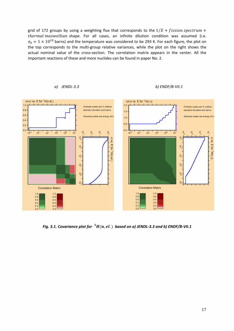
grid of 172 groups by using a weighting flux that corresponds to the 1⁄ shape. For all cases, an infinite dilution condition was assumed (i.e.
1 10 barns) and the temperature was considered to be 293 K. For each figure, the plot on
the top corresponds to the multi‐group relative variances, while the plot on the right shows the
actual nominal value of the cross‐section. The correlation matrix appears in the center. All the
important reactions of these and more nuclides can be found in paper No. 2.
a) JENDL‐3.3 b) ENDF/B‐VII.1
Fig. 3.1. Covariance plot for , . based on a) JENDL‐3.3 and b) ENDF/B‐VII.1
18
a) JENDL‐4 b) ENDF/B‐VII.1
Fig. 3.2. Covariance plot for , based on a) JENDL‐4 and b) ENDF/B‐VII.1
a) JENDL‐4 b) ENDF/B‐VII.1
Fig. 3.3. Covariance plot for , based on a) JENDL‐4 and b) ENDF/B‐VII.1
19
As seen in the previous figures, for each cross‐section of a given nuclide, the variability of the
probability of interaction at a certain energy group is related to the probability of interactions at
other energy groups since the same measuring equipment was used when determining such
probabilities. Such correlation can be studied through the self‐reaction covariance matrix. In the
same way, the variability of the probability of interaction at a certain energy group of a certain type
of reaction, is also related to the probability of interaction of a second type of reaction at the same
energy group due to the same reason as above. Such correlation can be studied through the multi‐
reaction covariance matrix.
An important issue that was noticed while computing the different reaction covariances was the fact
that resonance uncertainties in JENDL‐4 are absolute. This means that self‐shielded relative variances
(or relative standard deviations) will change as a function of temperature and dilution at the
resonant groups. This is illustrated in papers No. 1 and No.2, where relative standard deviations at
the resonant groups for different background cross‐sections were computed for the , and
, reactions. This fact is supported by the results obtained by Chiba et. al. [33], where a
dependency between relative multi‐group covariances and background cross‐sections at the
resonances was observed when JENDL‐3.2 data were employed. This is very important to take into
account when sampling the different isotopic reactions, because just as the nominal cross‐sections
are self‐shielded, their respective variances should be self‐shielded as well. However, JENDL‐4 data
does not exhibit a temperature‐dilution dependence of the variances at the resonances of important
actinides. Nevertheless, in this thesis, absolute variances at the resonances were self‐shielded,
assuming that the relative variances do not change as a function of temperature nor dilution.
Regarding the ENDF/B‐VII.1 resonant uncertainties, only an absolute dependency was observed,
leaving the relative terms intact for any temperature and/or dilution conditions. This is an important
issue, because as will be seen in the next sections, it is very easy to implement the perturbation
methodology based on relative uncertainties.
3.2 Determination of the sample size according to two‐group diffusion theory
Since uncertainty analysis in this work is performed on both and homogeneized two‐group
macroscopic cross‐sections, the minimum sample size to assess multivariate uncertainty based in
non‐parametric tolerance limits is dependent on the number of macroscopic cross‐sections that are
required to calculate . For example, by following the solution of the two‐group diffusion equation
in a homogenous system and applying vacuum boundary conditions [34], the well‐known four factor
formula can be derived:
Σ , Σ , ∙
Σ ,Σ
Σ ,
ΣΣ Σ ,
3.2
It is common that thermal up‐scattering is not present and thus, Σ Σ , → . Therefore, when
assessing the covariances between and the two‐group macroscopic cross‐sections, a minimum of
6 output parameters are in question (i.e. Σ , , Σ , , Σ , , Σ , , Σ , → and ). According to table
1b present in [26], for a two‐sided 95% coverage of 6 variables with a 95% of confidence, a minimum
of 361 samples are required. Nevertheless, if the uncertainty assessment is extended to other
parameters such as diffusion coefficients, a sample size of 410 elements is needed, because diffusion
coefficients are related to through the transport cross‐section. Therefore, since one of the main
goals of performing lattice calculations is to prepare a set of homogenized and energy collapsed
parameters for any further core analysis, the output sample for the multivariate uncertainty analysis
should contain at least 410 elements.
20
3.3 Main features of the DRAGON code and the DRAGLIB library
The DRAGON code is the result of an effort made at École Polytechnique de Montréal to rationalize
and unify the different models and algorithms used to solve the neutron transport equation into a
single code.
The management of a cross‐section library requires capabilities to add, remove or replace an isotope,
and the capability to reconfigure the burnup data without re‐computing the complete library. For
these purposes, DRAGR was developed by Hébert [30], and is an interface module to perform all
these functions while maintaining full compatibility with NJOY99 and its further improvements.
DRAGR produces DRAGLIB, a direct access cross section library in a self‐described format that is
compatible with DRAGON or with any lattice code supporting that format. The DRAGR Fortran
module was written as a clean and direct utility that makes use of the NJOY modules PENDF and
GENDF. For each nuclide within DRAGLIB, the cross‐sections for the following neutron‐interaction
Table 3.13. Uncertainty analysis of fast and thermal diffusion coefficients (ENDF/B‐VII.1)
Min. Value (cm) Max. Value (cm) Mean (cm) (cm)
Fast diffusion coefficient
1.42330 1.48890 1.45488 0.01123
Thermal diffusion coefficient
0.58439 0.58470 0.58474 0.00005
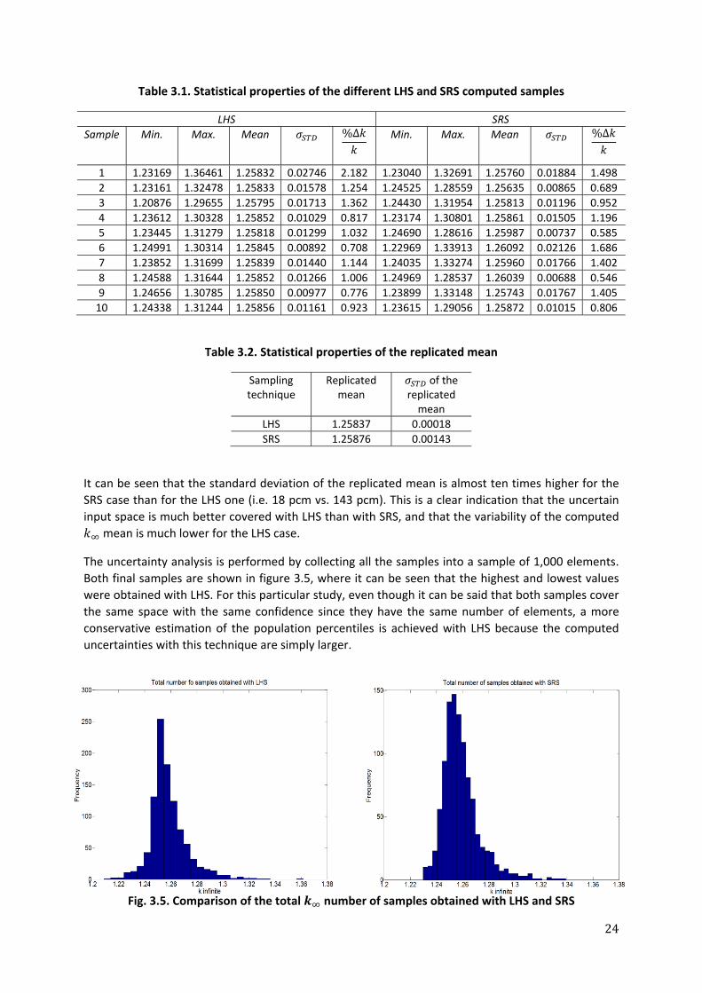
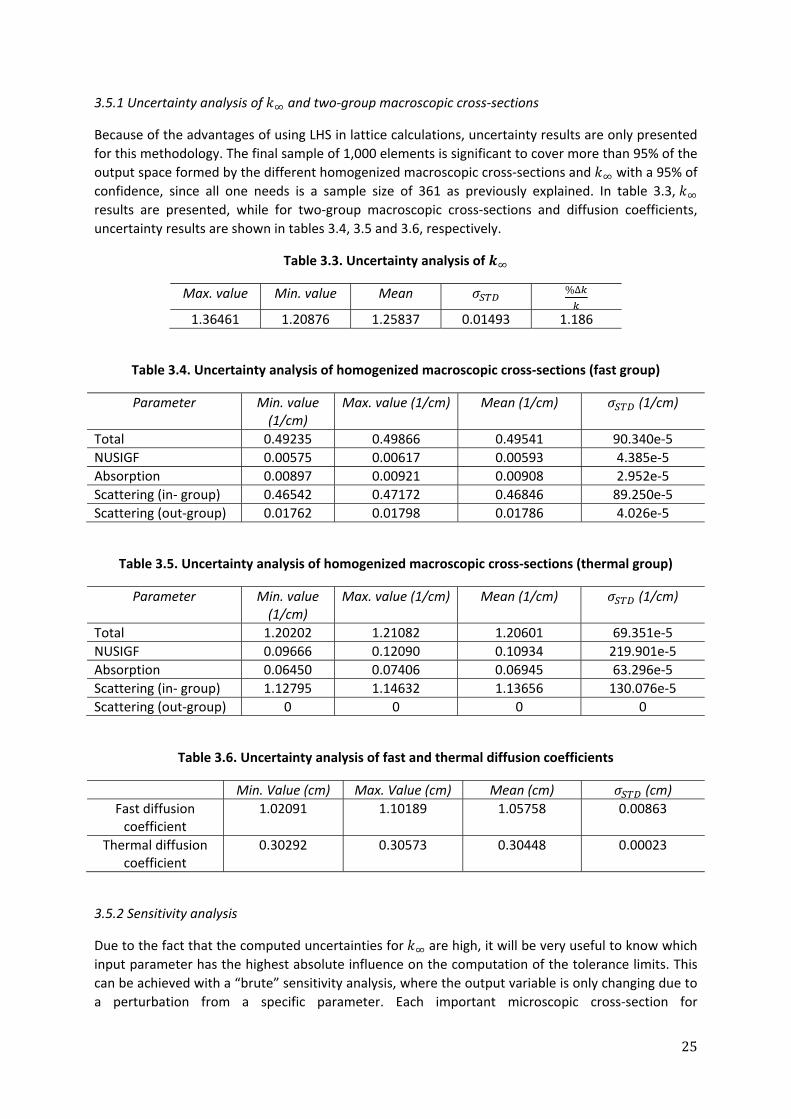
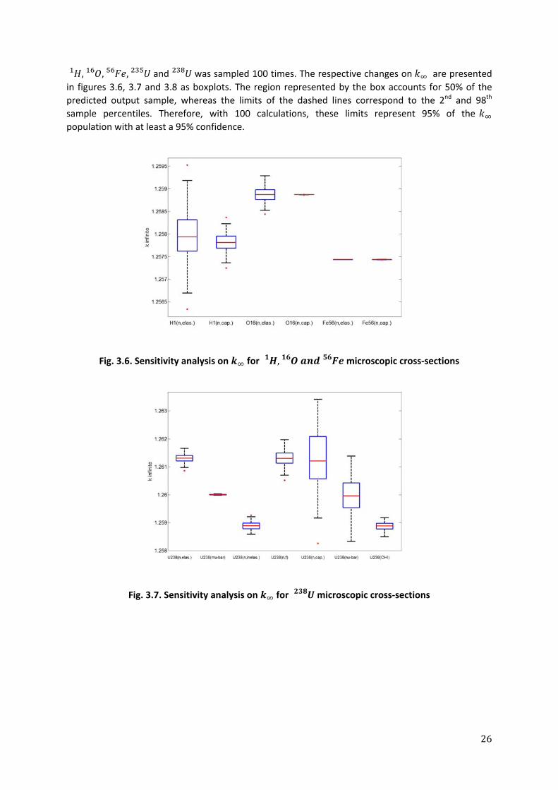
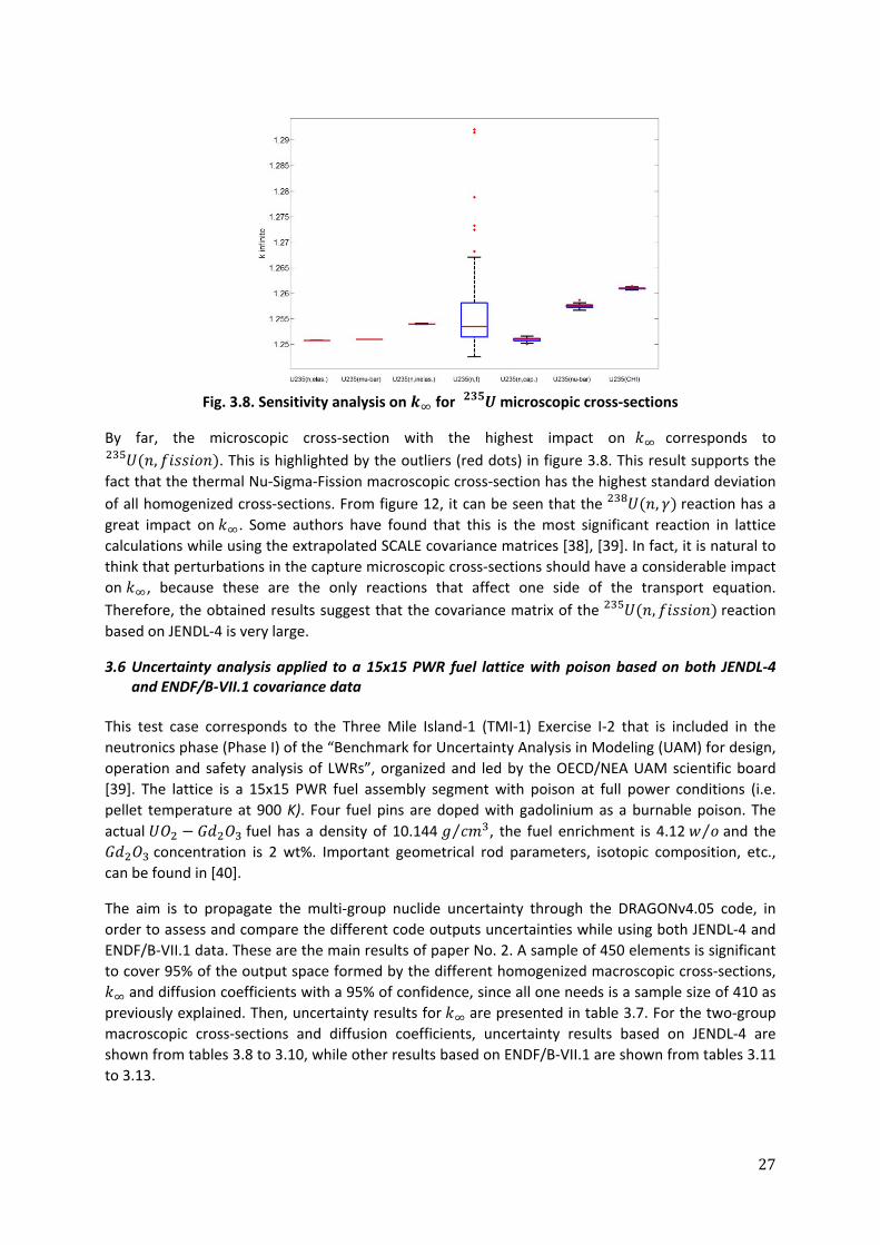
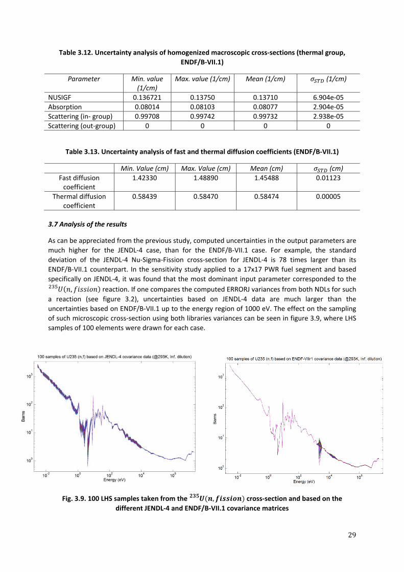
3.7 Analysis of the results
As can be appreciated from the previous study, computed uncertainties in the output parameters are
much higher for the JENDL‐4 case, than for the ENDF/B‐VII.1 case. For example, the standard
deviation of the JENDL‐4 Nu‐Sigma‐Fission cross‐section for JENDL‐4 is 78 times larger than its
ENDF/B‐VII.1 counterpart. In the sensitivity study applied to a 17x17 PWR fuel segment and based
specifically on JENDL‐4, it was found that the most dominant input parameter corresponded to the
, reaction. If one compares the computed ERRORJ variances from both NDLs for such
a reaction (see figure 3.2), uncertainties based on JENDL‐4 data are much larger than the
uncertainties based on ENDF/B‐VII.1 up to the energy region of 1000 eV. The effect on the sampling
of such microscopic cross‐section using both libraries variances can be seen in figure 3.9, where LHS
samples of 100 elements were drawn for each case.
Fig. 3.9. 100 LHS samples taken from the , cross‐section and based on the
different JENDL‐4 and ENDF/B‐VII.1 covariance matrices
30
A large difference is observed in the spread of the samples for thermal energies and almost up to the
last resonant energies. The fact of having large relative variances in JENDL‐4 for the thermal groups
(~ 7%) compared to small relative variances in ENDF/B‐VII.1 (~0.5%), and also large variance
differences (up to 10 times) at the resonances, is the cause of such a huge sampling variability
between both libraries.
Since uncertainties included in JENDL‐4 for , are very high compared with for
instance, the ones included in the ENDF/B‐VII.1 library, such a reaction becomes the most dominant.
As mentioned before, it is natural to think that capture cross‐sections has a big impact on lattice
calculations, since it is the only reaction that imbalance only one side of the neutron transport
equation (i.e. disappearance at a certain energy group). Nevertheless, unfair uncertainties among
different input reactions make the uncertainty computations to be very biased.
31
CHAPTER 4
FORWARD AND INVERSE UNCERTAINTY ANALYSIS APPLIED TO
NEUTRONIC CORE SIMULATORS
“Inside every nonBayesian there is a Bayesian
struggling to get out”
Dennis V. Lindley
During recent years, fuel loading strategies of many nuclear power plants have been based on best estimate (BE) calculations, allowing an optimization of the fuel depletion efficiency along the different cycles of the plant life. At the beginning of the pattern design of any plant cycle, a set of macroscopic cross‐sections are computed for the different fuel segment types that comprise each of the core fuel assemblies. As seen in chapter 3, such homogenized and energy‐collapsed macroscopic cross‐sections and diffusion coefficients can be obtained by means of a lattice code. Once these parameters are functionalized and discretized as a function of reactor state‐variables such as moderator temperature and density, fuel temperature, burnup, history variables, etc., they are used as inputs to the BE core simulators. In general, core simulators aim to solve the nodal two‐group diffusion equation in order to predict the spatial dependence of the scalar neutron flux at every burnup point within a cycle. This calculation is not only fundamental to achieve the desired energetic efficiency but also to ensure that the safety limiting parameters are never exceeded along the cycle, since the thermal flux is proportional to the produced thermal power. Ringhals 1 (R1) is an ASEA‐Atom Boling Water Reactor (BWR) located at the Ringhals power plant complex in western Sweden. It employs the Westinghouse POLCA7 core simulator for the design of the reactor fuel cycle, and utilizes the so‐called Core Master 2 (CM2) graphical interface to store and analyze the data of past and future cycles. CM2 is a practical tool where a view of the nodalized core is available, and nodal, assembly or core thermal‐hydraulic parameters, thermal margins, power and critical power ratio (CPR) (among others) are easily displayed. CM2 is part of the Westinghouse software for reactor analysis [41] that interacts and calls POLCA7 in order to calculate desired parameters at any burnup point within a cycle. 36 traversing incore prove (TIP) detectors are permanently positioned within the R1 core, and during each cycle a few TIP measurements at different burnup conditions are performed in order to estimate the actual spatial core neutron flux and thus, the core power and thermal margins. Therefore, the accuracy of core simulator calculations along the cycle can be assessed by computing the difference between predicted and measured quantities. Such procedure builds confidence in using the simulator for the long term fuel loading plans. In this chapter, two types of uncertainty analyses are performed on core simulations. The first one corresponds to the forward approach of input uncertainty propagation, where the input uncertain space formed by the nodal two‐group macroscopic cross sections and diffusion coefficients is sampled both with SRS and LHS. The possible ranges of variation of such input space are based on data from the depletion calculation corresponding to the cycle 26 of R1. The aim of this study is to compare the efficiency of the uncertainty assessment performed on the nodal thermal flux when SRS and LHS are employed. On the other hand, in the second type of uncertainty analysis presented in this chapter, discrepancies between spatial measured and calculated fluxes in R1 are used to perform an inverse uncertainty analysis on the spatial dependence of the different core parameters. This analysis is carried out using Bayesian statistics, where, for a certain cycle, the frequency distributions
32
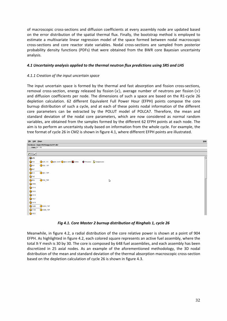
of macroscopic cross‐sections and diffusion coefficients at every assembly node are updated based on the error distribution of the spatial thermal flux. Finally, the bootstrap method is employed to estimate a multivariate linear regression model of the space formed between nodal macroscopic cross‐sections and core reactor state variables. Nodal cross‐sections are sampled from posterior probability density functions (PDFs) that were obtained from the BWR core Bayesian uncertainty analysis. 4.1 Uncertainty analysis applied to the thermal neutron flux predictions using SRS and LHS 4.1.1 Creation of the input uncertain space The input uncertain space is formed by the thermal and fast absorption and fission cross‐sections, removal cross‐section, energy released by fission , average number of neutrons per fission and diffusion coefficients per node. The dimensions of such a space are based on the R1‐cycle 26 depletion calculation. 62 different Equivalent Full Power Hour (EFPH) points compose the core burnup distribution of such a cycle, and at each of these points nodal information of the different core parameters can be extracted by the POLUT model of POLCA7. Therefore, the mean and standard deviation of the nodal core parameters, which are now considered as normal random variables, are obtained from the samples formed by the different 62 EFPH points at each node. The aim is to perform an uncertainty study based on information from the whole cycle. For example, the tree format of cycle 26 in CM2 is shown in figure 4.1, where different EFPH points are illustrated.
Fig 4.1. Core Master 2 burnup distribution of Ringhals 1, cycle 26
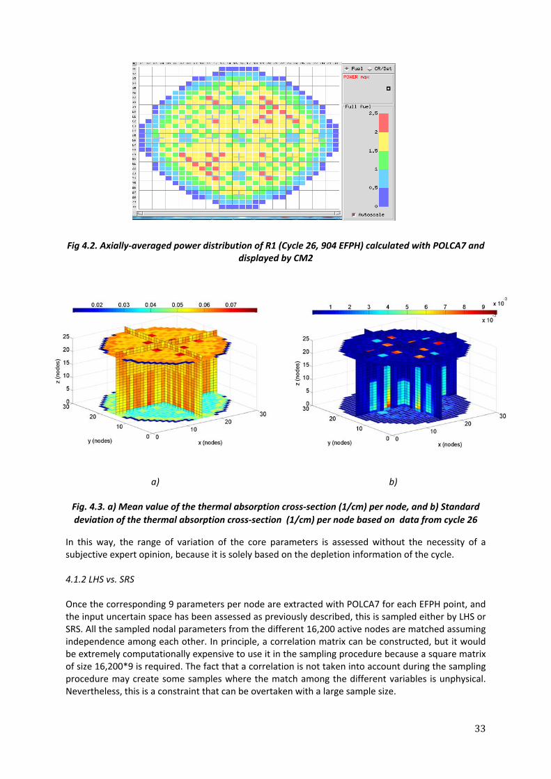
Meanwhile, in figure 4.2, a radial distribution of the core relative power is shown at a point of 904 EFPH. As highlighted in figure 4.2, each colored square represents an active fuel assembly, where the total X‐Y mesh is 30 by 30. The core is composed by 648 fuel assemblies, and each assembly has been discretized in 25 axial nodes. As an example of the aforementioned methodology, the 3D nodal distribution of the mean and standard deviation of the thermal absorption macroscopic cross‐section based on the depletion calculation of cycle 26 is shown in figure 4.3.
33
Fig 4.2. Axially‐averaged power distribution of R1 (Cycle 26, 904 EFPH) calculated with POLCA7 and
displayed by CM2
a) b)
Fig. 4.3. a) Mean value of the thermal absorption cross‐section (1/cm) per node, and b) Standard
deviation of the thermal absorption cross‐section (1/cm) per node based on data from cycle 26
In this way, the range of variation of the core parameters is assessed without the necessity of a subjective expert opinion, because it is solely based on the depletion information of the cycle. 4.1.2 LHS vs. SRS Once the corresponding 9 parameters per node are extracted with POLCA7 for each EFPH point, and the input uncertain space has been assessed as previously described, this is sampled either by LHS or SRS. All the sampled nodal parameters from the different 16,200 active nodes are matched assuming independence among each other. In principle, a correlation matrix can be constructed, but it would be extremely computationally expensive to use it in the sampling procedure because a square matrix of size 16,200*9 is required. The fact that a correlation is not taken into account during the sampling procedure may create some samples where the match among the different variables is unphysical. Nevertheless, this is a constraint that can be overtaken with a large sample size.
34
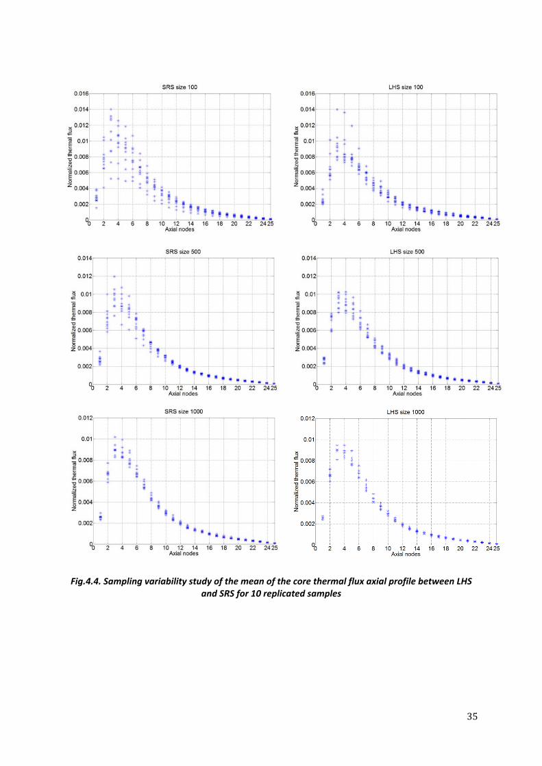
Once the input uncertain sample is created, this is propagated through an in‐house neutronic core simulator known as CORE SIM [42,43]. The calculations performed by this tool rely on the two‐group diffusion approximation, while the spatial discretization is based on finite differences. The coding was implemented in MatLab, which makes the pre‐ and post‐processing of data easy, as well as the code highly portable between different operative systems and computer platforms. For this particular study, the so called homogeneous or eigenvalue equations are solved. For this purpose, the explicitly‐restarted Arnoldi method is used so that the calculation of different eigenmodes is possible. In case of convergence problem, the user has also the possibility of choosing the power iteration method, which was implemented using Wielandt’s shift technique. The initial guess of the eigenvalues required for the application of Wielandt’s shift technique is provided by an Arnoldi run without restart. Although the accuracy of this tool cannot be compared to commercial core simulators, the tool offers several advantages such as: its ease of use, the robustness of the algorithms, and the fact that nonconventional systems can be easily investigated. Another main strength of the tool is that no input deck writing is required since only few data are required. In this section, results of the sampling variability studies made on cross‐sectional average quantities of the nodal thermal flux are shown below in figure 4.4. Ten replicates of the mean of the core axial profile of the thermal flux were computed for different sample sizes. As highlighted in figure 4.4, the variability of the replicated mean for the LHS case is less than the SRS case, especially at the lower part of the core where the averaged flux tends to peak the most. This is a clear indication that for a full core analysis of the thermal flux, the input uncertain space is being covered in a more efficient way when LHS is employed. As an example of the computed uncertainties on cross‐sectional average quantities of the nodal thermal flux, uncertainty limits obtained with LHS and SRS are shown in figure 4.5 when the sample size corresponds to 100 cases. Uncertainty limits correspond to the cross‐sectional average of the maximum values obtained for the nodal flux. As expected, the uncertainty limits obtained when LHS is employed are larger than the ones obtained by SRS at the lower part of the core. This is due to the fact that the flux is much more sensitive to the different changes of the macroscopic cross‐sections at the lower part than at the upper part of the core.
35
Fig.4.4. Sampling variability study of the mean of the core thermal flux axial profile between LHS
and SRS for 10 replicated samples
36
Fig. 4.5. Uncertainty analysis of the core averaged thermal flux axial profile for a sample size of 1000 cases both for SRS and LHS
In the uncertainty analysis applied to safety calculations of nuclear reactors, it is of particular interest to monitor the maximum value of the power throughout the core. Since the thermal power is proportional to the neutron flux, it can be a good idea to compute the possible maximum value of the thermal flux than can be achieved during an uncertainty analysis that is based on information from the whole cycle. Since a total of 16,000 core calculations were performed both with LHS and SRS, a convergence study was performed in order to analyze how many code runs are necessary so that the maximum value of the nodal flux within the core converges to a certain quantity. Such a study is shown in figure 4.6.
Fig. 4.6. Convergence analysis of the required number of runs for the convergence of the maximum value of the core nodal flux both for LHS and SRS
A much faster convergence towards the maximum value of the nodal thermal flux it can be seen for the LHS case, than for the SRS case. For instance, the maximum nodal thermal flux within the core has converged with LHS after 5,000 calculations, whereas for the SRS case it converges only after 8,000 calculations. This means that if we increase the sample size in order to cover as much as possible the probable input combinations, LHS will converge much faster than SRS to saturate all the probable permutations of the input variables and therefore, the output variables will not change their value anylonger. Also, the maximum value achieved with LHS for the normalized thermal flux corresponds to a value of 0.1233, while the maximum value achieved with SRS corresponds to a value of 0.120. This is a clear indication that the limits of the uncertainty assessment are more realistic when LHS is employed.
37
4.2 Bayesian uncertainty assessment of BWR core parameters based on flux measurements In this section, discrepancies between spatial measured and calculated fluxes in R1 are used to perform an inverse uncertainty analysis on the spatial dependence of core nodal parameters. This analysis is carried out using Bayesian statistics, where, for a certain cycle, the a priori distributions of the nodal macroscopic cross‐sections and diffusion coefficients at every assembly node are updated based on the error distribution of the spatial thermal flux. The first study of this kind was performed based on information from cycle 13 of R1, and published in paper No. 3 included in this thesis. In this section, results of the Bayesian uncertainty analysis based on information from R1‐cycle 26 are presented. As previously explained, the cycle No. 26 database of R1 consists of POLCA7 predictions performed at 62 different EFPH conditions, and for 14 of these EFPH points, TIP measurements are available. In reality, TIP detectors measure the reaction rate of the thermal flux. Since only 36 TIP detectors are radially located along the core, an unfolding methodology of the flux is required to estimate the spatial dependence of the measured flux. This methodology is included in the POLCA7 core simulator, and the final result of the unfolding algorithm [44] gives the nodal dependence of the measured thermal flux. Bayes theorem [45] states that the frequency of occurrence of random variables can be modified if some evidence that depends on such variable is available. Applying this concept to our particular case, a thermal flux error or evidence distribution that depends both on the measurements and calculations can be computed for each node and defined as | (where θ represents the nodal parameters). Such a distribution is used to update the simulator input parameters distributions (defined as ) through the following equation:
|||
4.1
Where | is the so called updated (or posterior) distribution of the nodal parameters. Assessment of the parameters and evidence distributions is described below. 4.2.1 Evidence distribution Since measurements were only performed at 14 different conditions along the cycle, nodal evidence distributions can only be assessed with 14 samples. It is common to assume that the distribution of the errors follows a normal distribution [46,47] mostly because in general, a normal distribution can approximate errors of various sources very well due to the central limit theorem [48]. Therefore, nodal samples of the error between measured and calculated thermal flux will be considered to be taken from a normal distribution. For instance, normality tests can be applied to any nodal sample of the error to confirm such a hypothesis. As an example, the flux error histogram for the top axial node of a fuel assembly located at the center of the core is shown in figure 4.7. A Lilliefors test was applied to such a sample in order to make a normality test. The p‐value of the test was 0.0023, so it can be significant not to reject the null hypothesis that the sample follows a normal distribution.
38
Fig. 4.7. Histogram of the discrepancies between predicted and measured thermal flux at the top
node of a central fuel assembly along cycle 26 4.2.2 Computation of the denominator of eq. 4.1 To update the parameter distributions, an integral over the whole domain of the parameters range per node should be computed. Due to the fact that this is a multidimensional function, an estimation of the integral of the product between all the inputs distributions and the evidence distribution is made through Marko Chain Monte Carlo (MCMC) integration. Using random walks and the Metropolis‐Hastings (M‐H) algorithm [49], numerical integration is possible. To generate a Markov chain in the parameter space, the M‐H algorithm is run by repeating a proposing step and a moving step. In each proposing step, the algorithm generates a new point on the basis of the previously accepted point with a proposal distribution ⁄ . In each moving step, the point is tested against the Metropolis criterion to examine if it should be accepted or rejected. If the is the targeted stationary distribution of | , a Matlab implementation of the M‐H algorithm can be done as follows:
1) Choose an arbitrary initial point in the parameter space.
2) (Proposing step). Propose a candidate point according to a proposal distribution ⁄ .
3) (Moving step). Calculate:
, 1, ⁄ ⁄
and compare the value with a random number from the uniform distribution U [0,1]. Set if , ; otherwise set . This is the Metropolis criterion. 4) Repeat steps 2 and 3 until enough samples are obtained.
The proposal distribution ⁄ can strongly affect the efficiency of the M‐H algorithm. To find an effective proposal distribution, it was required to make a first test run of the algorithm with 20,000 simulations using a uniform proposal distribution centered at the currently accepted point, such as:
(4.2)
39
Where is a random number uniformly distributed between 0 and 1, and and are the upper and lower values controlling the proposing step size. Based on the test run, a normal distribution 0, was constructed. Therefore, the following proposal distribution was adopted to
execute the MCMC simulations: 0, 4.3
In each proposing step of the M‐H algorithm a new point is generated from its predecessor from a normal distribution with mean , constant variances estimated from the previous run, and zero parameter covariance. The acceptance rates for the newly generated samples were about 30‐40% for a posterior 50,000 runs. 4.2.3 A‐posteriori nodal distributions of core parameters Posterior distributions of macroscopic‐cross sections and diffusion coefficiens per node are of interest. Based on a prior multivariate normal distribution, the ranges of the posterior PDfs are based on experimental data, and therefore, their associated uncertainties are computed based on information from a particular BWR cycle. In figure 4.8, a comparison between the prior and posterior distributions for some parameters are shown for the top node of the central fuel assembly.
Fig. 4.8. Comparison between prior and posterior PDFs of various nodal parameters based on data
from R1, cycle 26
It can be seen from the previous figure that posterior distributions are far away from being normal.
This technique is a good way of performing a realistic uncertainty analysis, since the probability
40
density functions of the input parameters of a core simulator are assessed without the need of
expert opinion.
4.3 Uncertainty analysis of a nodal cross‐section regression model by means of a non‐parametric
bootstrap method
Nodal macroscopic cross‐sections and diffusion coefficients depend on instantaneous and past
(history effects) conditions described by state variables such as burnup, thermal power, moderator
temperature and density, etc. Core simulators require nodal parameters as a function of many states
in order to calculate neutronic and thermal‐hydraulic variables in one or many cycles. One approach
to functionalize these dependences is through multivariate functions. Some of the existing models
are commonly built as a linear combination of suitable multivariate polynomials, where usually, a
unique set of regression coefficients are computed for various fuel depletion points and the
reconstructed nodal data are interpolated between the sampled fuel depletions. In general, each fuel
segment type uses the same polynomials to functionalize the different cross‐sections.
The fuel pattern analysis of R1‐cycle 26 was based on a depletion calculation performed at 62
different burnup points along the cycle. Since nodal state variables can be retrieved from POLCA7,
their respective cycle frequency distributions are based on samples of 62 elements. In this section,
the bootstrap method is employed to estimate a multivariate linear regression model of the space
formed between nodal macroscopic cross‐sections and core reactor state variables. This work is
presented in paper No. 4. Nodal cross‐sections are sampled from posterior probability density
functions (PDFs) that were previously obtained from a Bayesian uncertainty analysis. The idea is to
sample, from various nodes that are related to the same fuel segment, both the frequency
distributions of the nodal state variables and any posterior cross‐section PDFs in order to create the
following input‐output mapping:
, 4.4
Where , … , is the i‐th sample of the j‐th cross‐section, and is the matrix formed
by the different i‐th samples of the different 1,2, … , state varaibles, i.e.:
⋯
⋮ ⋱ ⋮⋯
4.5
Therefore, a relationship between any nodal macroscopic cross‐section and a few nodal state
variables from a specific fuel segment is analyzed through a multivariate regression analysis of the
form:
4.6
The , … , regression coefficients, which are bounded not only by the cycle information of
the state variables but also by the ranges of the posterior distributions of the macroscopic cross‐
sections, are derived with the bootstrap method. This is important due to the fact that such posterior
PDFs ranges are based on experimental data, and not anymore on expert opinion. The aim of this
work is to assess a degree of uncertainty to the regression coefficients by computing their respective
confidence intervals. Due to tremendous advances in modern computing capabilities, the non‐
parametric bootstrap method has been widely used in the statistical assessment of regression
parameters and their associated degree of variability [50]. In general, uncertainty analysis in reactor
calculations are performed to lattice and core simulators in a separate manner [51,52]. Although the
cross‐section models derived in this work are rather simple, the main goal is to point out the
41
importance of assessing uncertainty at all stages in the modeling of nuclear reactors, including
regression parameters that are used to functionalize macroscopic cross‐sections as a function of the
core state variables.
4.3.1 Creation of the input‐output space
Cross‐section models are used to arrange the different nodal core parameters in space as a function
of the state variables for the same type of fuel. Therefore, a specific model is assessed for a specific
fuel segment. In this work, a cross‐section model and its associated uncertainties are derived for a
fuel segment that is comprised between the 2nd and the 24th axial node of an ABB 10x10 SVEA96
assembly, located in the periphery of the core. Since 23 nodes comprise the fuel segment of interest,
the final sample of each state variable is composed by 1,426 elements. Therefore, the macroscopic
cross‐section being studied should be randomly sampled the same amount of times in order to
perform the linear multivariate regression analysis. In figure 4.9, the points defined by 1,426 samples
from the different removal cross‐section, burnup, fuel temperature, moderator density and
moderator density history PDFs are presented. These are the actual spaces that are going to be
bootstrapped in order to estimate the regression coefficients and their uncertainties.
a) b)
Fig. 4.9. Space defined by the samples obtained from the a) removal cross‐section, fuel
temperature and burnup and b) removal cross‐section, moderator density (instantaneous) and
moderator density (history)
4.3.2 Main features of the multivariate linear regression analysis
Regression analysis is a statistical technique that characterizes the relationship between two or more
variables for prediction and estimation by a mathematical model. Finding the variance of the
estimated coefficients, as well as constructing confidence intervals for is of main interest. In the
usual construction of a linear regression model for a certain that was obtained from the
1,… , samples such as:
4.7
it is assumed that the residuals are uncorrelated and normally distributed with zero
mean, i.e. ~ 0, . Furthermore, is assumed to be the same for all values of . It is the distributional assumption involving that allows the construction of statistical tests and parametric
42
confidence intervals for the coefficients [8]. For instance, if such assumptions are true and and
are defined such as:
⋮ , 1⋮1
⋯⋮ ⋱ ⋮
⋯ 4.8
The least square estimator given by:
4.9
has an associated variance‐covariance matrix and the following 100 1% confidence intervals [53]:
, ⁄ ∙ 4.10
Where , ⁄ is the t‐distribution with (n‐m) degrees of freedom, and is the standard
deviation of the coefficient.
Common statistical tests that are used to prove the significance of the regression coefficients
strongly rely on the aforementioned assumptions. If is the mean of the observations, an
approximation to can be derived as [8]:
∑
1 4.11
The well‐known F‐test statistic given by:
∑
4.12
Can be regarded as a randomly sampled value from an F‐distribution with (m,n‐m‐1) degrees of
freedom. This statistic can be used to test the accuracy of the constructed linear model, or, in other
words, to test that , … , 0.
Nevertheless, if the residuals distribution is unknown or difficult to derive, one cannot entirely rely
on the parametric approach to build linear regression models. For instance, if the residuals do not
follow a normal distribution, the F‐statistic does not follow an F distribution.
4.3.3 Bootstrap method
Bootstrapping is a non‐parametric and specific resampling technique that substitutes the traditional
distributional assumptions with computational effort. It offers a significant number of advantages
[54]:
Because it does not require any distributional assumption (such as normally distributed
errors), the bootstrap approach can provide more accurate inferences when the data are not
well behaved or when the sample size is small.
It is possible to apply the bootstrap to statistics with sampling distributions that are difficult
to derive, even asymptotically.
It is a general technique and relatively easy to implement with modern computational
resources.
43
One of the bootstrap methods that can be used in a linear regression analysis, and that is based on
the resampling of observations is described hereafter. This approach is applied when the coefficients
and the response of the regression model are considered random variables. The bootstrap procedure
based on the resampling of observation is as follows:
1) Draw independent bootstrap samples with replacement of the form , from
the estimated input‐output space defined by , . Thus, , , … , are
created.
2) Calculate the ordinary least square (OLS) coefficients from the bootstrap sample as follows:
4.13
3) Repeat steps 1 and 2 for r=1,…,B, where B is the number of repetitions.
4) Obtain the distribution from the bootstrap estimates , ,…, , and use
to estimate regression coefficients, variances, etc. Therefore, the bootstrap estimate
of the regression coefficient is the mean of the distribution [55]:
∑
4.14
Non‐parametric confidence intervals are easy to derive from the quantiles of the bootstrap sampling
distribution . By ranking the bootstrap , ,…, estimations, the 2⁄ % and
1 2⁄ % confidence interval for a certain coefficient is given by:
⁄ ⁄ 4.15
For example, if B=1000 replicates are taken and a 95% (i.e. 0.05) confidence interval of the b parameter is desired, once the bootstrap samples have been ordered, the 25th sample and the 975th
sample will give the corresponding upper and lower limits of the interval.
In addition to providing standard errors and confidence intervals, the bootstrap can also be used to
test statistical hypothesis. If we want to test if the computed coefficients , … , 0 , a bootstrap analysis can be performed in order to estimate the distribution of the test statistic. By
denoting F as the original F‐statistic of the input‐output space defined by , , the estimated
coefficients can be used to bootstrap the residuals and obtain, for each sample, an ∗‐statistic as
follows [55]:
1) Fit the regression model and obtain the residuals ⋯ from the original space.
2) For a single bootstrap iteration, obtain a bootstrap sample of the residuals and form a fix
, , … , bootstrap sample as previously explained. Compute the ∗ statistic
from Eq. 10.
3) Repeat step 2 many times for r=1,…,B.
Therefore, the bootstrap P‐value for the test of interest is the fraction of ∗ values that are
greater than or equal to the originally observed F‐value.
44
4.3.4 Results
Two cases will be studied, one corresponding to the mapping between the removal cross‐section,
burnup and fuel temperature and the other one corresponding to the mapping between the removal
cross‐section, moderator density and moderator density history, respectively. P‐values of the
hypothesis test 0: , … , 0, 95% confidence limits of the regression coefficients as well
as other statistical parameters of interest are presented. Each bootstrap sample consisted of 1,426
elements, a total of 10,000 replicates were performed in order to perform the different regression
analyses.
Case 1: Linear regression analysis on the input‐output space formed by the removal cross‐section,
burnup and fuel temperature
In table 4.1, a summary of the regression coefficients and their corresponding confidence intervals
are presented, while the corresponding ANOVA (Analysis of Variance) test of the regression analysis
is illustrated in table 4.2.
Table 4.1. Summary statistics of regression coefficients for case 1
Variables Related Coefficient Skewness of the distribution
95% Confidence Interval
Constant 0.0295 ‐0.0234 (0.0292,0.0297)
Burnup 1.530e‐05 ‐0.0013 (1.420,1.641)e‐05
Fuel Temp. ‐3.310e‐05 0.0176 (‐3.392,‐3.226)e‐05
Table 4.2. ANOVA results for case 1
Source DofF SS MS F P‐value
Regression 2 2.936e‐04 ‐ 3088.3 0.000
Residual 1423 7.354e‐05 4.754e‐08
R‐square=0.799
In figure 4.10, the estimated planes formed by the regression analyses 0.0292,0.02971.420,1.641 05 ∙ 3.392, 3.226 e 05 ∙ are shown, as well as all the observations
defined in the input‐output space of case 1.
45
Fig. 4.10. Uncertainty assessment of the regression analysis of case 1
Case 2: Linear regression analysis on the input‐output space formed by the removal cross‐section,
moderator density and moderator density history
In table 4.3, a summary of the regression coefficients and their corresponding confidence intervals
are presented, while the corresponding ANOVA (Analysis of Variance) test of the regression analysis
of this case is illustrated in table 4.4.
Table 4.3. Summary statistics of regression coefficients for case 2
Variables Related Coefficient Skewness of the distribution
95% Confidence Interval
Constant 0.0086 0.1219 (0.0079,0.0094)
Moderator Density 1.421e‐05 ‐0.1211 (1.322,1.521)e‐05
Moderator Density Hist. 0.166e‐05 0.0454 (0.157,0.175)e‐05
Table 4.4. ANOVA results for case 2
Source DofF SS MS F P‐value
Regression 2 2.818e‐04 ‐ 2554 0.000
Residual 1423 8.535e‐05 5.517e‐0888
R‐square=0.767
In figure 4.11, the estimated planes formed by the regression analyses 0.0079,0.00941.322,1.521 e 05 ∙ 0.157,0.175 e 05 ∙ are shown, as well as all the observations
defined in the input‐output space of case 2.
46
Fig. 4.11. Uncertainty assessment of the regression analysis of case 2
As early appreciated in figure 4.9, the space defined among the removal cross‐section, moderator
density and moderator density history for the fuel segment of interest, is more scattered and farther
away to be represented by a plane than the space defined by the removal cross‐section, burnup and
fuel temperature. Indeed, the ANOVA test for case 1 reflects a lower sum of the squares in the
residuals and a better R‐square ratio than case 2, which indicates that the space of case 1 fits better a
linear model than the space from case 2. Due to this fact, the computed confidence intervals for the
coefficients of the first case are relatively lower, than the computed confidence intervals for the
coefficients of the second case. Therefore, higher uncertainties are expected for regression models
that try to adjust a linear relationship among the different points of the sampled space.
The objective of this methodology presented is to estimate the uncertainty on the regression
coefficients used in cross‐section models. Although a very simple case was proposed in this chapter
where the coefficients are considered constant, the aim is to emphasize the importance of
performing uncertainty analysis at all the different stages in the modeling of nuclear reactors. For
instance, cross‐sections models are very important because they are the link between thermal‐
hydraulic calculations and core simulators.
47
CHAPTER 5
UNCERTAINTY AND SENSITIVITY ANALYSES APPLIED TO THERMAL‐
HYDRAULIC CALCULATIONS
“If nuclear power plants are safe, let the commercial insurance industry insure
them. Until these most expert judges of risk are willing to gamble with their
money, I'm not willing to gamble with the health and safety of my family”.
Donna Reed
While the licensing regulations were being codified, an international effort was initiated in parallel
to:
a) Develop BE codes with the capability to calculate accurate values of the key phenomena that
restrict plant operational limits;
b) Obtain data to enable validation and verification of the system analysis codes;
c) Perform code validation and verification to ensure that the capabilities of the code are
known and acceptable.
Such a need to validate and refine BE codes that are used in the predictions of relevant reactor safety
parameters, led to the organization of international benchmarks based on high quality experimental
data. The OECD/NRC BWR Full‐Size Fine‐Mesh Bundle Test (BFBT) benchmark was established in
2002 based on available data from the Nuclear Power Engineering Corporation (NUPEC) in Japan, and
offers a good opportunity to assess the accuracy of thermal‐hydraulic codes in predicting, among
other parameters, single and two phase bundle pressure drops, cross‐sectional averaged void
fraction distributions and critical powers under a wide range of system conditions. With respect to
the void distribution inside a fuel assembly, which has been regarded as an important factor in the
determination of boiling transition in boiling water reactors (BWRs), NUPEC performed from 1987 to
1990 a series of radial void measurements at four axial locations in a full‐size mock‐up test facility
able to simulate the high pressure, high temperature fluid conditions found in BWRs through
electrically‐heated rod bundles. Therefore, since other important parameters such as system
pressure, inlet sub‐cooling and power input conditions were also supplied, these test series form a
substantial database for the assessment of the accuracy of thermal hydraulic codes in predicting
radial and axial assembly void distributions, under both steady‐state and transient conditions.
Nevertheless, due to uncertainties coming from, e.g. approximations in the physical models,
variation and imprecise knowledge of initial and boundary conditions, scatter of measured
experimental data, etc., it has been recognized in the last years that uncertainty analysis would not
only be necessary if useful conclusions are to be obtained from BE calculations, but would also
complete the validation process of BE codes [56].
The work presented in this chapter has two main objectives. The first one is to enhance the
validation process of the thermal‐hydraulic features of the Westinghouse code POLCA‐T. This is
achieved by computing a quantitative validation limit based on statistical uncertainty analysis. This
validation theory is applied to some of the benchmark cases of the following macroscopic BFBT
exercises, based on a one dimensional model of the NUPEC ITF:
1. Exercise 0, Phase II. Steady‐state single and two phase pressure drops
48
2. Exercise 2, Phase I. Steady‐state cross‐sectional averaged void fraction
3. Exercise 3, Phase I. Transient cross‐sectional averaged void fraction
4. Exercise 1, Phase II. Steady‐state critical power benchmark
Sensitivity analysis is also performed to identify the most important uncertain parameters for each
exercise.
The second objective consists in showing the clear advantages of using the quasi‐random Latin
Hypercube Sampling (LHS) strategy over simple random sampling (SRS). For cross‐sectional averaged
void fraction predictions under both steady‐state and transient conditions, a comparison between
statistical uncertainty analyses by means of LHS and SRS is presented. The aim is to show that the
replicated void fraction mean (either in steady‐state or transient conditions) has less variability when
using LHS than SRS for the same number of calculations (i.e. same input space sample size) even if
the resulting void fraction axial profiles are non‐monotonic.
5.1 Description of the NUPEC test facility
The facility is able to simulate the high pressure, high temperature fluid conditions found in nuclear
reactors. An electrically‐heated rod bundle has been used to simulate a full scale BWR fuel assembly.
In the test section, the simulated full scale BWR fuel assembly was installed within a pressure vessel.
Two bundle types, a “current 8x8 type” and a “high burn‐up 8x8 type” were simulated. Three types
of axial power profiles were used: uniform, cosinusoidal and inlet peak. Also, different radial power
distributions were achieved through different pin power factors.
Two types of void measurement systems were employed as shown in figure 5.1: an X‐ray computed
tomography (CT) scanner and an X‐ray densitometer. Under steady‐state conditions, fine mesh radial
void distributions were measured using the X‐ray CT scanner located 50 mm above the heated
length. The attained spatial resolution was as small as 0.3 mm X 0.3 mm. However, the X‐ray
densitometer measurements of void distributions around each rod were performed at three
different axial elevations from the bottom (i.e. 682 mm, 1706 mm and 2730 mm) under both steady‐
state and transient conditions. For the each of the four different axial locations, the cross‐sectional
averaged void fraction was also measured.
Fig. 5.1. Void fraction measurement system
49
Absolute and differential pressures were measured using diaphragm transducers. The inlet flow rate
was measured using a turbine flow meter, and the inlet sub‐cooling was measured using double
thermistors. Table 5.1 shows the estimated measurement accuracy of these process parameters.
Table 5.1. Accuracy (%) of the main processes that were recorded
Quantity Accuracy
Pressure 1 %
Flow 1 %
Power 1.5 %
Inlet fluid temperature 1.5Cross‐sectional
averaged void fraction 2%
The BFBT offers the possibility to benchmark averaged cell void fraction predictions under two types
of simulated transient scenarios: a half re‐circulation pump trip, and a half turbine trip without
bypass. The “half” scenario means that after some time from the occurrence of the corresponding
transient, nominal operating conditions were fed again into the fuel assembly in order to avoid rod
cladding damages. In a pump trip scenario, the core mass flow rate is suddenly decreased, exposing
the coolant left in the core to a sudden increase of temperature and therefore, to a sudden increase
in the void fraction. Regarding the turbine trip case, a sudden increase on the outlet pressure will
collapse the coolant void. In a real BWR, this will increase the neutron moderation leading to a power
increase and ergo, leading to a sudden increase on the void fraction. For these purposes, the code
used time dependent boundary and power input conditions artificially created and released by
NUPEC, which are shown in figure 5.2.
a) b)
Fig. 5.2. Boundary and input power conditions representing the a) half recirculation pump trip, and
b) half recirculation turbine trip
In contrast to the CT scanner, the X‐ray densitometers were not rotating but fixed during a
measurement. Thereby, a pencil type beam was shot through a certain alley of sub‐channels
between two neighboring rod rows. As discussed in [57], because of this principle only parts of the
sub‐channel cross‐sections have been scanned in between the rod rows. Therefore, sub‐channel
0 20 40 607
7.05
7.1
7.15
7.2x 10⁶
Time [s]
Out
. Pre
ssur
e [P
a]
0 20 40 600
5
10
15
20
Time [s]
Flo
w R
ate
[kg/
s]
0 20 40 60280
281
282
283
Time [s]
Inle
t Tem
pera
ture
[deg
-C]
0 20 40 602.5
3
3.5
4
4.5x 10⁷
Time [s]
Pow
er [W
]
0 20 40 607
7.5
8
8.5x 10⁶
Time [s]
Out
. Pre
ssur
e [P
a]
0 20 40 608
10
12
14
16
Time [s]
Flo
w R
ate[
kg/s
]
0 20 40 60280.5
281
281.5
282
Time [s]
Inle
t Tem
pera
ture
[deg
-C]
0 20 40 602
4
6
8x 10⁶
Time [s]
Pow
er [W
]
50
center effects are overestimated while near wall effects are neglected. Depending on the prevailing
flow regime two opposite phenomena led to systematic measurement errors.
In case of high void fractions the vapor concentration in the sub‐channel center is higher than near
the walls (slug and churn flow regime). Therefore, a higher average void fraction than in reality was
measured. Because of the systematic deviations of the densitometer measurements, Aydogan et. al
[58] developed correlations in order to correct the experimental values. Since the two types of fuel
assemblies used for the measurements have different flow areas, two different correlations were
derived. Such correlations should correct X‐ray densitometers void fraction measurements that lie
between 20% and 90%. These are illustrated in Eqs. 5.1 and 5.2.
For the current 8x8 assembly:
,
0.001 , 1.231 5.1
For the high burn‐up 8x8 assembly:
,
0.001 , 1.167 5.2
For both transient scenarios, the fuel assembly simulating high burn‐up conditions was employed
with a uniform axial power profile. The three different axial positions of the X‐ray densitometers
correspond to the calculations given by nodes 19th, 12th and 5th, respectively, of the POLCA‐T output
deck. For both transient scenarios, Eq. (5.2) was applied in order to have the correct void fraction
measurements.
5.2 Description of the POLCA‐T system code
The Westinghouse transient code POLCA‐T is a three‐dimensional coupled simulator solving for the
thermal‐hydraulic and neutronic fields. The code is used mainly for transient analysis of BWRs. The
thermal‐hydraulic part of the code [59] corresponds to a 5‐equation model based on the
conservation equations of mass and energy for gas and liquid phases, and on the conservation
equation of momentum for the mixture. For each defined control volume cell, values of pressure,
phase enthalpies and phase masses are determined by the solution of the conservation equations.
The most important constitutive relations are friction and local pressure drop correlations, critical
flow correlations and a drift‐flux model employed to solve the velocities of the two phases for all
flow regimes. For the BFBT benchmark, the drift‐flux Holmes correlation was chosen. The thermal
model calculates the heat conduction and heat transfer from the heat structures to the coolant.
Equations are resolved in Eulerian coordinates, where a fully implicit numerical method is employed
to solve the hydraulic model and the simultaneous heat transfer and thermal conduction equations.
Since the main process parameters measured in the integral test facility (ITF) are available in the
database, the test fuel assembly was modeled in POLCA‐T (version 1.6.0/T5‐1.9.0) as a one‐
dimensional BWR channel considering as boundary conditions the inlet fluid temperature, the mass
flow rate and the assembly outlet pressure. The seven spacers were modeled with constant K‐loss
coefficients to take into account local pressure drops. In order to model the axial power profile, a
heat structure was used to combine the effects of all heated rods. Thus, radial pin power factors
were not taken into account. The channel nodalization was set to 24 equidistant axial volumes of
0.154 m in length, assigning the nodes numbering from bottom to top from 1 to 24, respectively, as
shown in figure 5.3.
51
Fig. 5.3. BFBT equivalent model in POLCA‐T
5.3 Statistical uncertainty analyses of void fraction predictions using LHS and SRS
This section focuses on the results of sampling variability studies and uncertainty analyses performed
with LHS and SRS on predicted cross‐sectional averaged void fractions. The estimations are for both a
steady‐state condition and a simulated re‐circulation pump trip scenario. These results constitute a
summary of paper No. 5.
The most important sources of uncertainty that are present in the BFBT benchmark were identified
by the different organizers and participants, and can be found in [60]. By the use of “expert opinion”,
a PDF and standard deviation was assigned to each parameter. The uncertain input space for this
section is based on 8 parameters that are directly available in the POLCA‐T input deck. Four of them
correspond to the boundary and power input conditions released by NUPEC, and their probabilistic
assessment was based on their experimental accuracy. Two parameters correspond to important
geometrical parameters such as the hydraulic diameter and the total flow area, whereas the last
parameters correspond to the rod cladding surface roughness and spacer K loss coefficient,
respectively. The K loss factor was set to a value of 0.94, and the rod roughness was considered to be
2.5 , according to some changes in the BFBT specification and stated in [61]. Table 5.2 describes
the assessment of the uncertain input space for further uncertainty analyses.
52
Table 5.2. Input space uncertain parameters
Parameter PDF Mean Stand. Dev.
Pressure Normal Nominal 1%
Flow rate Normal Nominal 1%
Inlet temperature
Uniform Nominal 1.5
Power Normal Nominal 1.5%
Hydraulic diameter
Normal 1.295 1%
Flow area Normal 97.81 1%
Roughness Normal 2.5 5%
Spacer K loss
coefficient
Normal 0.94 5%
5.3.1 Steady‐state case
The nominal values of the boundary conditions corresponding to the BFBT 0021‐18 steady‐state test
case are shown in table 5.3.
Table 5.3. Nominal conditions for the steady‐state test case
Parameter Nominal value
Pressure 7.17Flow rate 15.37 ⁄
Inlet temperature 279Total power 3.5
For the sampling variability study between LHS and SRS, ten replicates of the axial void fraction
profile mean were computed for different sample sizes. Figure 5.4 shows the results of such a study,
where it can be noticed that in all four cases LHS performs much better than SRS. It should be noted
that the axial void fraction profile forms a monotonic function.
53
0 1 2 3 40
20
40
60
80
Voi
d f
ract
ion
[%
]Assembly height [m]
LHS size 7
0 1 2 3 40
20
40
60
80
Voi
d f
ract
ion
[%
]
Assembly height [m]
SRS size 7
0 1 2 3 40
20
40
60
80
Voi
d f
ract
ion
[%
]
Assembly height [m]
LHS size 30
0 1 2 3 40
20
40
60
80
Voi
d f
ract
ion
[%
]
Assembly height [m]
SRS size 30
0 1 2 3 40
20
40
60
80
Voi
d f
ract
ion
[%
]
Assembly height [m]
LHS size 50
0 1 2 3 40
20
40
60
80
Voi
d f
ract
ion
[%
]
Assembly height [m]
SRS size 50
0 1 2 3 40
20
40
60
80
Voi
d f
ract
ion
[%
]
Assembly height [m]
LHS size 100
0 1 2 3 40
20
40
60
80
Voi
d f
ract
ion
[%
]
Assembly height [m]
SRS size 100
Fig. 5.4. Sampling variability study between LHS and SRS for 10 mean replicates (Steady‐state)
5.3.2 Transient case
Uncertainty analysis is presented on the transient case corresponding to the half re‐circulation pump
trip scenario. Since for this case the boundary and input power conditions are time dependent, a
protocol to sample the input space should be followed. POLCA‐T is designed to handle transient
cases in an easy way; for instance, a file containing a look‐up table of any parameter as a function of
time can be defined. Thereby, at every specific time defined in the table, the nominal value of the
parameter is considered to be the mean value and from its characteristic PDF, the required sample is
taken. Boundary and input conditions are defined in the input deck of the code every second and
thus, at every second there exists a particular sample from the input space.
As for the steady‐state case, a sampling variability study is presented in figure 5.5 for the predicted
time‐dependent cross‐sectional averaged void fraction at the axial location of 687 mm (same location
as the lowest densitometer). Ten replicates of void fraction mean were computed for different
54
0 20 40 600
10
20
30
40
50
Vo
id f
ract
ion
[%
]
Time [s]
LHS size 7
0 20 40 600
10
20
30
40
50
Vo
id f
ract
ion
[%
]
Time [s]
LHS size 30
0 20 40 600
10
20
30
40
50
Vo
id f
ract
ion
[%
]
Time [s]
SRS size 7
0 20 40 600
10
20
30
40
50
Vo
id f
ract
ion
[%
]
Time [s]
SRS size 30
0 20 40 600
10
20
30
40
50
Voi
d f
ract
ion
[%
]
Time [s]
LHS size 50
0 20 40 600
10
20
30
40
50
Voi
d f
ract
ion
[%
]
Time [s]
LHS size 100
0 20 40 600
10
20
30
40
50
Voi
d f
ract
ion
[%
]
Time [s]
SRS size 50
0 20 40 600
10
20
30
40
50
Voi
d f
ract
ion
[%
]
Time [s]
SRS size 100
sample sizes. It can be seen that, even if the void fraction is not monotonic in time, LHS performs
much better than SRS.
Fig. 5.5. Sampling variability study between LHS and SRS for 10 mean replicates (transient)
5.4 Uncertainty and sensitivity analysis as a validation tool
In this section, statistical uncertainty and sensitivity analyses are used to validate the thermal‐
hydraulic features of the POLCA‐T code, based on a one dimensional model of some test cases of the
BFBT macroscopic exercises. A methodology to set validation limits is derived from both
measurement and code uncertainty. The results shown below are a summary of the paper No. 6.
55
5.4.1 Overall validation methodology
The error is the difference between a simulated or an experimental value and the truth. Since
accuracy indicates the closeness of agreement between a simulated/experimental value of a quantity
and its true value, accuracy increases as error approaches zero. However, the true values of
simulated/experimental values are rarely known and thus, errors must be estimated.
For our particular case, since validation is the process of assessing simulation uncertainty by using
benchmark experimental data, it would be necessary first to estimate the errors involved in the
measurement systems of the different parameters included in table 3.1. It is natural to consider that
measurement errors follow a normal distribution and thus, they can be estimated with a certain
degree of confidence. It was agreed in the benchmark specifications for uncertainty analysis [61],
that a generic measurement standard deviation can be obtained by multiplying the nominal
measurement by its accuracy, i.e.:
∙ % 5.3
Therefore, following a normal distribution, a generic uncertainty would estimate an error with a
95% of confidence if it is calculated as:
2 5.4
Once both the experimental ( and the simulation or code ( ) uncertainty have been computed,
a validation uncertainty can be defined as the combination of all uncertainties that can be
estimated as:
5.5
If the absolute value of the error between the prediction and the experiment defined as:
| | | | 5.6
is less than the validation uncertainty , it can be said that validation has been achieved at the
level. Then, is the key metric in the validation process and it is imposed by the uncertainties
inherent in the experiments, the numerical solution and the model input space [62].
5.4.2 Results of the uncertainty and sensitivity analyses
In this section, the results of the uncertainty and sensitivity analysis on the different BFBT exercises
are presented. For each specific exercise, the parameters considered to be the most important
sources of uncertainty and that are directly available in the input deck are indentified, defining a
particular uncertain input space. To each of these parameters, a PDF is assigned using expert opinion.
For the simulation uncertainty analysis of each test case, the size of the uncertain input space sample
is 100. The upper and lower predicted uncertainty limits correspond to the 99th and 1st percentiles of
the output sample, respectively. These limits represent a 95‐95% confidence interval of the possible
values of the code output population. Measurement uncertainty is also present at each case and it is
computed from Eqs. (5.3) and (5.4). On the other hand, sensitivity analysis is only performed in a
selected test. In this case, 100 samples are taken from each source of uncertainty in order to
evaluate which parameter has the greatest effect on the code output.
56
Ex. 0, Phase II. Steady‐state single phase pressure drop exercise
For this exercise, a PDF was assigned to 5 important uncertain parameters. Table 5.4 describes the
assessment of this particular uncertain input space, where the mean of each parameter PDF
corresponds to the values used in the nominal calculation.
Table5.4. Sources of uncertainty considered for the single phase pressure drops exercise
Parameter PDF Mean Stand. Dev.
Flow rate Normal Nominal 1%
Hydraulic diameter
Normal 1.295 1%
Flow area Normal 97.81 1%
Roughness Normal 2.5 5%
Spacer K loss
coefficient
Normal 0.94 5%
Six different tests were selected for the study, where the boundary conditions for each case are
shown in table 5.5. For the pressure transducer experimental uncertainty, a standard deviation of 1%
of the nominal measurement was considered. The benchmark with uncertainty analysis for each test
can be appreciated in figure 5.6, where the horizontal blue bar corresponds to the measurement
uncertainty, while the vertical blue bar corresponds to the code uncertainty. It can be seen that all
nominal predictions lie within the [‐10%,+10%] band, and that the code has the tendency to under‐
predict the bundle pressure drop tests. Regarding the validation process for each test case, a
comparison between the absolute error and the validation uncertainty can be found in table 5.5. In
all cases, the absolute prediction error was less than the validation uncertainty. Thus, the code
predicts bundle single phase pressure drops accurately for a wide range of mass flow rates.
57
20 25 30 3515
20
25
30
35
40
Measured pressure drop [kPa]
Pre
dict
ed p
ress
ure
drop
[kP
a]
M/P=1+10%-10%Nominal Prediction
P70035
P70034
P70036
28
29
30
31
32
33
Mass flow Hyd. Diam. Flow Area Rough. Spacer loss
Pre
dict
ed p
ress
ure
drop
[kP
a]
Fig. 5.6. Single phase pressure drops benchmark Fig. 5.7. Sensitivity analysis of single phase
uncertainty analysis pressure drops (P70036 test)
Table 5.5. Nominal conditions and validation limits of the single phase pressure drops tests
Test. No. Outlet Pressure (MPa)
Inlet Temp.
Mass flow rate (kg/s)
Reynolds number 10
| | (MPa) (MPa)
P70027 7.15 284.9 5.64 8.07 0.291 0.346
P70028 7.16 285.1 6.92 9.91 0.397 0.506
P70029 7.16 285.1 8.28 11.86 0.460 0.683
P70034 7.15 284.8 16.59 23.74 0.980 1.445
P70035 7.16 284.6 18.00 25.76 0.770 2.041
P70036 7.15 284.8 19.42 27.79 0.878 2.001
Sensitivity analysis was performed on test P70036. In figure 5.7, a group of boxplots show how the
pressure drop changes to each parameter defined in the uncertain input space. The box accounts for
50% of the predicted output sample, whereas the limits of the dashed lines correspond to the 2nd and
98st sample percentiles. These represent approximately 90% of the output pressure drop population
with 100 calculations. Finally, if the maximum and/or minimum values of the sample do not fit
between the limits of the dashed lines, they are considered outliers and are exposed as stars.
As expected, the spacer K loss coefficient is shown to have a great effect on the pressure drop since it
dominates local losses predictions. Other two important geometric parameters are the flow area and
hydraulic diameter, since these have a great impact on the friction pressure drop. Therefore, it can
2 3 4 5 6 71
2
3
4
5
6
7
8
Measured pressure drop [kPa]
Pre
dict
ed p
ress
ure
drop
[kP
a]
M/P=1+10%-10%Nominal Prediction
P70027
P70028
P70029
58
be concluded that the wall friction and local pressure loss models are well implemented and accurate
enough.
Ex. 0, Phase II. Steady‐state two phase pressure drop exercise
Accurate predictions of two phase pressure drop are fundamental for a proper determination of the
momentum continuity equations and therefore, are fundamental for accurate predictions of
averaged void fractions in BWR calculations.
For this exercise, a PDF was assigned to 7 important uncertain parameters as described in table 5.6.
Table 5.6. Sources of uncertainty considered for the two phase pressure drops exercise
Parameter PDF Mean Stand. Dev.
Flow rate Normal Nominal 1%
Inlet temperature
Uniform Nominal 1.5
Power Normal Nominal 1.5%
Hydraulic diameter
Normal 1.295 1%
Flow area Normal 97.81 1%
Roughness Normal 2.5 5%
Spacer K loss
coefficient
Normal 0.94 5%
Six different tests with a cosinusoidal axial power profile were selected for the study, where the
boundary conditions for each case are shown in table 5.7. The selected power range is between
0.863 MW and 6.478 MW. The first three tests correspond to a low mass flow rate condition, while
the last three correspond to a nominal BWR bundle flow rate condition. The benchmark with
uncertainty analysis for each test can be appreciated in figure 5.8.
It can be seen that all nominal predictions lie within the [‐10%,+10%] band. The code under predicts
the two phase pressure drops of the low flow rate cases; however, for nominal BWR flow rates, it
predicts the bundle two phase pressure drop reasonably well (difference smaller than 1.5%). A
comparison between the absolute error and the validation uncertainty can be found in table 5.7. In
all cases, the absolute prediction error was less than the validation uncertainty. Thus, the code
predicts bundle two phase pressure drops accurately both for a wide range of power and flow rate
conditions.
Sensitivity analysis was performed on test P60011, and it is shown in figure 5.9. It can be seen that
the flow area is the parameter having the biggest influence on the pressure drop correlation when a
two phase flow condition is present. Also, as seen in the previous exercise, the spacer K loss
coefficient is also an important factor in the constitutive pressure drop correlation. Regarding the
effect of the three perturbed boundary conditions, the three are more or less equally important to
the code pressure drop model.
59
25 26 27 28 29 3020
21
22
23
24
25
26
27
28
29
30
Measured pressure drop [kPa]
Pre
dict
ed p
ress
ure
drop
[kP
a]
M/P=1+10%-10%Nominal Prediction
P60001
P60003
P60005
50 60 70 80 90 100 11050
60
70
80
90
100
110
120
Measured pressure drop [kPa]
Pre
dict
ed p
ress
ure
drop
[kP
a]
M/P=1+10%-10%Nominal Prediction
P60007
P60009
P60011
104
105
106
107
108
109
110
111
112
113
Mass flow In. Temp. Hyd. Diam. Flow Area Power Rough. Spacer loss
Fig. 5.14. Uncertainty analysis of the pump trip Fig. 5.15. Uncertainty analysis of the turbine trip
Regarding the analysis of the turbine trip, it is observed that all the measurement points from
densitometer No. 1 and 2 are within the predicted 95% tolerance interval with at least a 95% of
confidence. However, during the time interval from 18 to 50 seconds, the nominal measurement
from densitometer No. 3 falls outside the predicted limits, demonstrating that the code over predicts
63
the void fraction by up to 12%. The absolute errors of the three points lying outside the validation
uncertainty can be found in table 5.9.
Table 5.9. Points lying outside the validation uncertainty from densitometer No. 3 (Turbine trip)
Time (s)
| |(%) (%)
48 20.968 20.034
49 20.830 20.548
50 21.151 19.126
Finally, just like in the pump trip case, it can be concluded that the code captures the qualitative
behavior of the turbine trip very well during the whole transient.
Ex. 1, Phase II. Steady‐state critical power benchmark
The uncertain input space for this exercise is defined in table 5.10, where a PDF was assigned to 7
parameters.
Table 5.10. Sources of uncertainty considered for the critical power benchmark (Steady‐state)
Parameter PDF Mean Stand. Dev.
Outlet pressure
Normal Nominal 1%
Flow rate Normal Nominal 1%
Inlet temperature
Uniform Nominal 1.5
Hydraulic diameter
Normal 1.295 1%
Flow area Normal 97.81 1%
Roughness Normal 2.5 5%
Spacer K loss
coefficient
Normal 0.94 5%
The four test cases requested by the benchmark organizers for the uncertainty analysis [60] are
presented hereafter. Boundary conditions are described in table 5.11, where it can be seen that such
conditions are very different for each test case. To all of them, a cosinusoidal axial power profile was
applied. For the power experimental uncertainty, a standard deviation of 1.5% of the nominal
measurement was considered. The uncertainty analysis is shown in figure 5.16.
It can be appreciated that not all the benchmarked tests lie within the [‐10%,+10%] band, the code
over predicting the critical power for the majority of the cases. This is due to the fact that the flux‐
quality correlation is tuned to work properly under BWR nominal conditions, just like test SA603901,
whereas other tests are far from nominal BWR conditions. Another conclusion from this study is the
fact that the code is not too sensitive to the defined uncertain input space, since for all cases the
predicted uncertainty is not larger than 1.6%.
64
2 4 6 8 10 12
2
4
6
8
10
12
14
Measured critical power [MW]
Pre
dict
ed c
ritic
al p
ower
[MW
]
M/P=1+10%-10%Nominal Prediction
SA512800
SA812800
SA505900
SA603901
Sensitivity analysis was performed on test SA812800, and the results are shown in figure 5.17. It can
be noticed that the most relevant parameter is the inlet sub‐cooling boundary condition, which is
crucial (as seen before in the void fraction case) to the boiling transition point.
Table 5.11. Nominal conditions and validation limits of the critical power tests
Test. No. Outlet Pressure (MPa)
Inlet Temp.
Mass flow rate (kg/s)
Initial Power (MW)
Exp. Critical Power (MW)
| | (MW) (MW)
SA603901 7.18 282.75 2.78 1.5 3.2 0.050 0.346
SA505900 5.49 264.69 5.59 3.5 5.980 0.948 0.458
SA812800 8.67 275.66 18.13 6.5 8.90 0.483 0.571
SA512800 5.50 242.8 18.20 8.5 11.09 1.395 0.642
Fig. 5.16. Critical power benchmark uncertainty analysis
Fig. 5.17. Sensitivity analysis of critical power benchmark (SA812800 test)
9.3
9.32
9.34
9.36
9.38
9.4
9.42
9.44
9.46
Press. Mass flow In. Temp. Hyd. Diam. Flow Area Rough. Spacer loss
Pre
dict
ed c
ritic
al p
ower
[MW
]
65
CHAPTER 6
CONCLUSIONS AND FUTURE WORK
“If you follow reason far enough it always leads to conclusions
that are contrary to reason.”
Samuel Butler
In this work, uncertainty analysis is performed at every stage in the modeling of LWRs, in an ongoing
effort made by the nuclear community to rely on the simulations performed by neutronic and
thermal‐hydraulic BE codes. The statistical approach for performing uncertainty analysis based on
Latin Hypercube sampling proved to be more efficient in the coverage of input uncertainties than
simple random sampling. This is one of the first works that employs LHS to sample the input
uncertain space, and then uses the concept of non‐parametric tolerance intervals for the code
output uncertainty assessment in both neutronic and thermal‐hydraulic calculations. It was shown at
every stage in the modeling of LWRs that LHS offers the possibility to assess more realistically non‐
parametric tolerance limits than SRS, because code non‐linearities are much better handled when
the input space is covered in an efficient way. Therefore, the combination of both LHS and non‐
parametric statistical coverage of the code output space is valid, because such a theory solely relies
on the ranking of the output sample and the size of such a sample. In principle, there should not be
concern about using LHS in the code output uncertainty assessment while this one is being based on
the theory of non‐parametric tolerance intervals.
A summary of the main achievements and general conclusions is given as follows:
In chapter 3, uncertainty analysis was applied to lattice calculations of the DRAGONv4.05
code. It was found that the computed uncertainties of , homogeneized and energy‐
collapsed macroscopic cross‐sections and diffusion coefficients based on JENDL‐4 data are
much larger than for instance, computed uncertainties based on ENDF/B‐VII.1 data. This is
one of the first attempts to compute and propagate multi‐group microscopic cross‐section
uncertainty from newly released nuclear libraries through lattice codes. Also, it is one of the
first attempts to perturb the DRAGLIB library, which is compatible with advance self‐shielding
models used in deterministic lattice calculations.
In chapter 4, a statistical uncertainty analysis was performed on nodal thermal flux
calculations of a full BWR core. From a simple Monte Carlo‐based strategy of input
uncertainty propagation, it was shown that LHS converged much faster to compute the
maximum possible value of the nodal thermal flux along the core than SRS. The dimension of
the input uncertain space was based on the cycle 26 depletion calculation of the Ringhals 1
BWR. On the other hand, a Bayesian approach was used to infer posterior distributions of the
different nodal parameters based on actual flux measurements performed along cycle 26 of
R1. Even though the ranges of such posterior PDFs could only be based on evidence
distributions obtained for a full cycle, such a theory opens the possibility to infer parameter
uncertainty based on real experiments and not anymore on expert opinion. Emphasis was
made on performing uncertainty analysis at all possible modeling stages, including the
coefficients of a nodal cross‐section model. Although a very simple model was derived, the
66
aim is to propose an uncertainty assessment based on replicated sampling techniques such
as the general bootstrap method.
The ongoing efforts to validate BE thermal‐hydraulic codes widely used in the nuclear
industry were enhanced with the uncertainty and sensitivity analysis presented in chapter 5.
Based on the different exercises of the BFBT benchmark, it can be said that the POLCA‐T code
is very accurate in predicting steady‐state pressure drops and cross‐sectional averaged void
fractions under a wide range of conditions, where the absolute error of all test cases was
below the validation uncertainty. Regarding the transient analyses, the qualitative behavior
of the code tracked very well the measured void fraction, and only three comparison errors
were found to be slightly higher than the validation limit on the turbine trip scenario. Finally,
regarding the critical power exercise, four different tests with very different nominal
conditions were analyzed. This fact has a big impact on the code accuracy since the critical
power ratio (CPR) model is designed to work with nominal BWR pressure conditions. This
explains why the absolute errors of the two low pressure test cases were higher than the
validation uncertainty.
The present study performs a realistic analysis of nuclear reactors, particularly in the uncertainty
prediction of important neutronic and thermal‐hydraulic LWR parameters at different stages of the
calculations. Nevertheless, the nature of the different parameter uncertainties were not coupled in
this work. State‐of‐the art calculations require the use of coupled codes in order to fully apply the BE
concept of multi‐physics modeling. The key aspect for handling uncertainties in coupled calculations
is to first compute the uncertainties in the cross‐sections models, because they are the link between
neutronic and thermal‐hydraulic predictions. In this thesis, it was shown that the uncertainties of
these models are accounted in their respective coefficients. Even though statistical uncertainty
analysis relies on first principles, some research still needs to be done on how to implement it at all
modeling stages for coupled calculations.
67
REFERENCES
[1]. OECD, International Atomic Energy Agency (IAEA). “Uranium 2011: Resources, Production and Demand”,
ISBN: 9789264178038, pp. 408, (2012).
[2]. International Atomic Energy Agency (IAEA). “Best Estimate Safety Analysis for Nuclear Power Plants:
Uncertainty Evaluation”, Safety Reports Series No. 52, (2008).
[3]. Nuclear Regulatory Comission (NRC). Domestic Licensing of Production and Utilization Facilities, Code of Federal Regulations 10, Part 50 NRC, Washington D.C., (1995). [4]. International Atomic Energy Agency (IAEA). “Safety Assessment and Verification for Nuclear Power Plants”, IAEA Safety Standards Series No. NS‐G‐1.2, Vienna, (2001). [5]. Helton J. C., Davis F. J. “Latin hypercube sampling and the propagation of uncertainty in analyses of complex systems”, Realiability Eng. & System Safety, Vol. 81, pp. 23‐69, (2003). [6]. International Atomic Energy Agency (IAEA). “Safety of Nuclear Power Plants: Design”, IAEA Safety Standards Series No. NS‐R‐1, Vienna, (2000). [7]. International Atomic Energy Agency (IAEA). “Safety of Nuclear Power Plants: Operation”, IAEA Safety Standards Series No. NS‐R‐2, Vienna, (2000). [8]. Helton J., Davis F.J. “Sampling‐Based Methods for Uncertainty and Sensitivity Analysis”, SANDIA REPORT
SAND99‐2240, pp. 1‐101, (2000).
[9]. Hernández‐Solís A. “Uncertainty and sensitivity analysis applied to the validation of BWR bundle thermal‐hydraulic calculations”, Chalmers University of Technology, Licentiate Thesis, CTH‐NT‐231, pp. 49, (2010). [10]. Glaeser H. “GRS Method for Uncertainty and Sensitivity Evaluation of Code Results and Applications”, Science and Technology of Nuclear Installations, Vol. 2008, pp. 1‐6, (2008). [11]. Harper F.T., Breeding R.J., Brown T.D. “Evaluation of severe accident risks: Quantification of major input parameters. Expert opinion elicitation on In‐Vessel Issues”, NUREG/CR‐4551, SAND86‐1309 Vol. 2., (1990). [12]. Electric Power Research Institute (EPRI). “Probabilistic seismic hazard evaluations at Nuclear power plant sites in the central and eastern United States”, NP‐6395D, (1989). [13]. Booker J.M., Anderson M.C., Meyer M. “The role of expert knowledge in uncertainty quantification (Are we adding more uncertainty or more understanding?)”. Los Alamos Nat. Lab. Report, (To be published). [14]. Petruzzi A. “Development and Application of Methodologies for Sensitivity Analysis and Uncertainty Evaluation of the Results of the Best Estimate System Codes Applied in Nuclear Technology”, PhD thesis, University of Pisa, etd‐11082008‐094257, (2008). [15]. McKay MD, Beckman RJ, Conover WJ. “A comparison of three methods for selecting values of input
variables in the analysis of output from a computer code”, Technometrics, Vol. 21 (2), (1979).
[16]. Iman R. L., Conover W. J. “A distribution‐free approach to inducing rank correlation among input
variables”, Commun. Stat.‐ Simula. Computa., B11 (3), pp. 311‐334, (1982).
[17]. Glaeser H., Hofer E., Kloos M., Skorek T. “Uncertainty and sensitivity analysis of a post‐experiment calculation in thermal hydraulics”, Reliability Eng. & System Safety, Vol. 45 (1‐2), pp. 19‐33, (1994).
68
[18]. Wilks S. S. “Determination of sample sizes for setting tolerance limits”, Annals of Mathematical Statistics, Vol. 12 (1), pp. 91‐96, (1941). [19]. Wilks S. S. “Statistical prediction with special reference to the problem of tolerance limits”, Annals of Mathematical Statistics, Vol. 13 (4), pp. 400‐409, (1942). [20]. Wilks S. S. “Mathematical Statistics”, Wiley Ed., New York, (1962). [21]. Wald A. “An extension of Wilks’ method for setting tolerance limits”, Annals of Mathematical Statistics, Vol. 14, pp. 44‐55, (1943). [22]. Wald A., Wolfowitz J. “Tolerance limits for a normal distribution”, Annals of Mathematical Statistics, Vol. 17, pp. 208‐215, (1946). [23]. Guba A., Makai M., Pal L. “Statistical aspects of best estimate method‐I”, Reliability Eng. & System Safety, Vol. 80 (3), pp. 217‐232, (2003). [24]. Noether G.E. “Elements of Nonparametric Statistics”, Wiley Ed., New York, (1967). [25]. Scheffe H., Tukey J.W. “A formula for sample sizes for population tolerance limits”, Annals of Mathematical Statistics, Vol. 15 (2), pp. 217, (1944). [26]. Ackermann H, Abt K. “Designing the sample size for non‐parametric, multivariate tolerance regions”. Biometrical Journal, Vol. 26 (7), pp. 723‐734, (1984). [27]. McKay, M.D. “Uncertainty Analysis, Chapter 4”, Yigal Ronen, CRC Press, 1st. Ed., pp. 296, (1988). [28]. Matala A. “Sample Size Requirement for Monte Carlo – Simulations using Latin Hypercube Sampling”, 60968 Internal Report, Dep. of Eng. Phys. and Math., Helsinki University of Technology, pp. 1‐24, (2008). [29]. Macfarlane R. E., Kahler A. C. “Methods for Processing ENDF/B‐VII with NJOY”, Nuclear Data Sheets, Vol. 111, pp. 2739‐2890, (2010). [30]. Hébert A. “A nuclear data library production system for advanced lattice codes”, International Conference on Nuclear Data for Science and Technology, pp. 701‐704, (2007). [31]. Chiba G. “ERRORJ – A Code to Process Neutron‐nuclide Reaction Cross Section Covariance, Version 2.3”, JAEA‐Data/Code 2007‐007, (2007). [32]. Kosako K. et. al. “Preparation of a Covariance Processing System for the Evaluated Nuclear Data File, JENDL (III)”, JNC TJ9440 99‐003, (1999). [33]. Chiba G., Ishikawa M. “Revision and Application of the Covariance Data Processing Code, ERRORJ”, International Conference on Nuclear Data for Science and Technology, pp. 468‐471, (2005). [34]. Stacey W. M. “Nuclear Reactor Physics”, Wiley – VCH, Germany, (2004). [35]. OECD/NEA Databank. “ERRORJ, Multigroup covariance matrices generation from ENDF‐6 format”, Package No. NEA‐1676/07, (2010). [36]. Marleau G., Hébert A. “A User Guide for DRAGON 3.06”, École Polytechnique de Montréal, IGE–174 Rev. 7 Report, (2008). [37]. Khan A. A., Lye L., Husain T. “Latin hypercube sampling for uncertainty analysis in multiphase modeling”, Journal of Environmental Eng. & Science, Vol. 7 (6), pp. 617‐626, (2008).
69
[38]. Ball M. “Uncertainty Analysis in Lattice Reactor Physics Calculations”, McMaster University, PhD Thesis No. 6565, (2012). [39]. Pusa M. “Incorporating sensitivity and uncertainty analysis to a lattice physics code with application to CASMO‐4”, Annals of Nuclear Energy, Vol. 40, pp. 153‐162, (2012). [40]. Ivanov K. et. al. “Benchmark for Uncertainty Analysis in Modeling (UAM) for Design, Operation and Safety Analysis of LWRs vol. I: Specification and Support Data for the Neutronic Cases (Phase I)”, NEA/NSC/DOC(2011), Version 2, (2011). [41]. Muller E. “CoreLink Methodology”, Westinghouse Electric Sweden AB report, BCM 98‐040 rev 9, pp. 69, (2007). [42]. Demazière C. “Description of the models and algorithms used in the CORE SIM neutronic tool”, Chalmers University of Technology CTH‐NT‐241 report, pp. 33, (2011). [43]. Demazière C. “User’s manual of the CORE SIM neutronic tool”, Chalmers University of Technology CTH‐NT‐243 report, pp. 24, (2011). [44]. Lindahl S. “POLCA7‐Detector Adapted Power Distribution and Thermal Margins (UPDAT)”, Westinghouse Electric Sweden AB report, BCM 97‐211 rev 3, pp. 14, (2008). [45]. Lee P. “Bayesian statistics: An introduction” Wiley, 3rd. Ed., ISBN 978‐0‐470‐68920‐2, (2009).
[46]. Braswell B.H., Sacks W.J., Linder E., Schimel D.S. “Estimating diurnal to annual ecosystem parameters by synthesis of a carbon flux model with eddy covariance net ecosystem exchange observations”, Global Change Biol., Vol. 11, pp. 335–355, (2005). [47]. Raupach M.R., Rayner P.J., Barrett D.J., Defries R.S., Heimann M., Ojima D.S., Quegan S., Schmullius C.C. “Model data synthesis in terrestrial carbon observation: methods, data requirements and data uncertainty specifications”, Global Change Biol., Vol. 11, pp. 378–397, (2005). [48]. Von Mises R., “Mathematical Theory of Probability and Statistics”, Elsevier, New York, (1964). [49]. Gelfand A.E., Smith A.F.M. “Sampling‐based approaches to calculating marginal densities”, Journal of the American Statistical Assoc., Vol. 85, pp. 398–409, (1990). [50]. Effron B. “More Efficient Bootstrap Computations”, Journal of the American Statistical Assoc., Vol. 86, pp. 79‐89, (1990). [51]. Macian R., Zimmermann M., Chawla R. “Statistical Uncertainty Analysis Applied to Fuel Depletion Calculations”, Nuclear Science and Technology, Vol. 44 (6), pp. 875‐885, (2007). [52]. Anchel F. et. al. “Uncertainty and sensitivity analysis in the neutronic parameters generation for BWR and