Uncertainty of the X-ray Diffraction (XRD) sin2 ψ Technique in Measuring Residual Stresses of Physical Vapor Deposition (PVD) Hard Coatings

LUO, Quanshun <http://orcid.org/0000-0003-4102-2129> and YANG, Shicai

Available from Sheffield Hallam University Research Archive (SHURA) at:

http://shura.shu.ac.uk/16586/

This document is the author deposited version. You are advised to consult the publisher's version if you wish to cite from it.

Published version

LUO, Quanshun and YANG, Shicai (2017). Uncertainty of the X-ray Diffraction (XRD) sin2 ψ Technique in Measuring Residual Stresses of Physical Vapor Deposition (PVD) Hard Coatings. Coatings, 7 (8), 128-18.

Copyright and re-use policy

See http://shura.shu.ac.uk/information.html

Sheffield Hallam University Research Archivehttp://shura.shu.ac.uk

coatings

Article

Uncertainty of the X-ray Diffraction (XRD) sin2 ψ

Technique in Measuring Residual Stresses of PhysicalVapor Deposition (PVD) Hard Coatings

Quanshun Luo 1,* and Shicai Yang 2

1 Materials and Engineering Research Institute, Sheffield Hallam University, Howard Street,

Sheffield S1 1WB, UK2 Miba Coating Group, Teer Coatings Ltd., West Stone House, West Stone, Berry Hill Industrial Estate,

Droitwich, Worcestershire WR9 9AS, UK; shicai.yang@miba.com

* Correspondence: q.luo@shu.ac.uk; Tel.: +44-114-2253649

Received: 3 July 2017; Accepted: 17 August 2017; Published: 20 August 2017

Abstract: Residual stresses of physical vapor deposition (PVD) hard coatings can be measured using

X-ray diffraction (XRD) methods under either conventional d-sin2 ψ mode or glancing incident

(GIXRD) mode, in which substantial uncertainties exist depending on the applied diffraction

parameters. This paper reports systematic research on the effect of the two analytical modes, as well

as the anisotropic elastic modulus, on the measured residual stress values. A magnetron sputtered

TiN grown on hardened tool steel was employed as the sample coating, to measure its residual stress

using various diffraction peaks from 111 to 422 acquired at a range of incident glancing angles

from 2 to 35. The results were interpreted in terms of the effective X-ray penetration depth, which

has been found to be determined predominantly by the incident glancing angle. In the d-sin2 ψmode,

the results present an approximate residual stress over a depth of effective X-ray penetration, and it

is recommended to use a diffraction peak of high-index lattice plane from 311 to 422. The GIXRD

mode helps determine a depth profile of residual stress, since the measured residual stress depends

strongly on the X-ray penetration. In addition, the anisotropy of elastic modulus shows limited

influence on the calculated residual stress value.

Keywords: PVD hard coatings; residual stresses measurement; X-ray diffraction

1. Introduction

Most hard coatings grown by plasma enhanced physical vapor deposition (PVD) show various

levels of residual stresses which strongly influence the adhesion and tribological performance.

Accordingly, accurate stress measurement is highly desirable. Similar requirements also exist in many

other engineering materials, such as surface-hardened turbine blades, gears and spring components.

X-ray diffraction (XRD) is a widely used method of residual stress measurement, namely, by

means of the XRD sin2 ψ technique [1–4]. A schematic sketch of the method is shown in Figure 1.

A crystalline plane is employed as the strain gauge to measure its d-spacing at a series of off-axis

angles, ψ, i.e., the angle between the normal of the strain gauge plane to the normal of the sample

surface. Then by plotting the d-spacing linearly against the corresponding sin2 ψ values, a linear

regression is made whereas the slope is used to calculate the lattice strain. In the conventional sin2 ψ

measurement, a crystal plane, usually having a high diffraction angle (2θ > 125), is selected as the

strain gauge that a series of ψ angles can be obtained by acquiring its diffraction peaks at different

incident angles, Ω, of the X-ray beam [4,5]. For thin films or coatings, however, the measurement

at such a large diffraction angle always comes with an extremely weak diffraction peak and strong

peak broadening. Consequently, crystalline planes of low diffraction angles have also been used.

Coatings 2017, 7, 128; doi:10.3390/coatings7080128 www.mdpi.com/journal/coatings

Coatings 2017, 7, 128 2 of 16

An alternative method is glancing incident XRD (GIXRD), in which a constant Ω angle of incident

X-ray is employed to acquire diffraction peaks of different diffraction angles and thereafter different

ψ angles, given the relation between the three angles as ψ = θ − Ω [6–12]. The GIXRD method is

especially useful in measuring the residual stresses of extremely thin films and surface layers when a

very low Ω angle is employed. The GIXRD method has been useful in measuring the residual stresses

of thin films and coatings having cubic crystalline structures [9,11,13–16].

ψ ψ θ − Ω

Ω

A schematic diagram showing the geometric set‐up of X‐ray diffraction (XRD)

ψ ‐ ψ ‐ ψ

ψ ‐ ψ

ψ ‐ Ω

ψ ‐ ‐

‐

‐

‐ ψ

‐ ψ ‐

Ω

Figure 1. A schematic diagram showing the geometric set-up of X-ray diffraction (XRD) residual

stress measurements.

Large uncertainties may arise in residual stress measurements when the applied XRD sin2 ψ

method results in either a nonlinear d-sin2 ψ plot or large scattering in a linear d-sin2 ψ plot. In the

conventional sin2ψ measurement, for example, Perry and co-workers reported splitting sin2 ψ plots in

measuring the residual stresses of sputtered titanium nitride coatings by using the 220, 111 and 200

planes [8]. Kim reported different slopes of the sin2 ψ plots between the measurements using 111

and 200 crystal planes of titanium nitride coatings [7]. For the former, the uncertainties may result

from both the dependence of X-ray penetration on the applied diffraction geometry, i.e., the Ω and

ψ angles and the structural heterogeneity of the films and coatings to be measured. In fact, different

crystalline planes, from the low-index planes 111 and 200, to the high-index planes 311 to 422,

have been employed by many researchers in measuring the residual stresses of TiN coatings [8–11].

Similarly, in the GIXRD method, the incident angle has been also known to have remarkable influence

on values of the measured residual stresses because of the variation of X-ray penetration depth [10,12].

Unfortunately, there is a lack of systematic experimental research to clarify and interpret the effect of

these geometric factors on stress measurements, although being discussed in theoretical principal [13].

For the latter, because the nano-scale structure heterogeneity of PVD coatings has been experimentally

approved as a result of microstructure evolution during their growth, a stress profile is expected to

exist along the depth of such a coating. Related to this, theoretical and experimental approaches have

been published for the measurement of stress profiles [17–19].

In addition, the anisotropic nature of most crystalline materials also leads to considerable scatter of

the calculated stress values because the Young’s modulus depends on the crystallographic orientation.

In case of transition metal nitrides, a number of papers reported the anisotropic elastic modulus of

titanium nitride coatings [8,20–24]. For the data scattering in a linear d-sin2 ψ plot, it has been reported

that the method of diffraction peak positioning has significant influence on the precision of the linear

d-sin2 ψ regression and the parabolic method was recommended to give the lowest scattering [25].

In this paper, an assumption of orientation-independent biaxial stress state has been followed

to allow the study to be focused on the uncertainties of residual stress measurements arising from

the selection of XRD parameters. For this purpose, a magnetron sputtered titanium nitride coating

Coatings 2017, 7, 128 3 of 16

has been selected as a sample coating to investigate the effect of XRD geometry on the results of

residual stress measurement. A series of Ω angles have been employed to acquire diffraction peaks

of crystal planes of the nitride ranging from 111 to 422. In particular, the diffraction angles of

most of the employed crystal planes are lower than 125, the minimum angle for high-accuracy stress

measurements recommended in the literature [4,5]. To interpret the obtained results, the relationship

between the X-ray penetration depth and the intensity of the diffracted X-ray beam has been calculated

as a function of the applied geometrical conditions. It is expected that the results presented could

help improve understanding about the accuracy in XRD residual stress measurements, especially the

selection of appropriate diffraction parameters.

2. Experimental Procedure and Stress Calculation

2.1. The Sample Material

A stoichiometric titanium nitride coating was grown on a polished coupon surface of pre-hardened

(HRC 64) M42 tool steel, by using a four-magnetron close-field unbalanced magnetron sputtering

system (self-made equipment, Teer Coatings Ltd., Droitwich, UK). In the reactive sputtering deposition,

all the four pure titanium targets were powdered under direct-current magnetron mode where the

deposition chamber was maintained with partial pressure of gaseous nitrogen. The deposition

procedures started with argon-ion etching on the samples using a pulsed DC power of frequency

350.0 kHz, pulse width 0.5 µs and a high negative substrate potential of −400 V. Then a thin metallic

titanium interlayer, approximately 230 nm thick, was grown at a substrate bias −70 V and the four

magnetrons being powered at 3.0 kW. After that, reactive nitrogen gas was introduced to deposit the

stoichiometric TiN for 40 min.

Details of the structural characterization and mechanical properties of the sample coating can be

found elsewhere [26]. In brief, the coating was 2.56 µm thick, exhibiting a single-phase cubic crystalline

structure with a strong 220 texture and hardness of HK0.025 34.8 ± 3.8 GPa. Figure 2a,b shows

the surface morphology of the coating and its microstructure, respectively. In Figure 2a, the coating

exhibits a rough surface in sub-micron scale, whereas in Figure 2b the cross-sectional TEM (transmission

electron microscopy, CM 20 STEM, Philips, Eindhoven, The Netherlands) micrograph shows dense

columnar TiN grains. Note that the Ti interface is shown at the bottom of the cross-sectional micrograph,

as labelled in Figure 2b.

‐

‐ ‐

‐ ‐ ‐ ‐

‐

‐ −

−

‐

‐ ‐

‐

(a) (b)

Figure 2. (a) A FEG‐SEM (field‐emission‐gun scanning electron microscopy) micrograph of the TiN ‐

‐ ‐ α θ θ

Figure 2. (a) A FEG-SEM (field-emission-gun scanning electron microscopy) micrograph of the TiN

coating surface; (b) A cross-sectional TEM bright field micrograph of the TiN coating.

2.2. XRD Experiments

A computer programmed Philips X’Pert X-ray diffraction instrument (Almelo, The Netherlands)

was employed, using an incident radiation of Cu-Kα1 (λ = 0.154056 nm, the copper anode at 40 kV and

Coatings 2017, 7, 128 4 of 16

40 mA). Figure 1 shows the XRD setup of residual stress measurements. The instrument was run with

a PW3050/60 goniometer which could perform both under the θ/2θmode and the glancing angle (GA,

or Ω-2θ) mode with minimum step size of 0.001. In this work, the incident X-ray was in line-focus

and aligned to pass a divergence slit and an anti-scattering slit, both of 0.25, and a mask window of

10 mm in width. No monochromator was applied so that a fraction of Cu-Kα2 (λ = 0.1544426 nm) was

also included in the incident beam in addition to the Cu-Kα1. In particular, before each XRD scan, the

height position of the sample to be analyzed was carefully adjusted using a manufacturer-supplied dial

gauge which has a height resolution of 0.002 mm. Diffraction curves were acquired at the Ω-2θmode.

In this mode, while the incident X-ray hits the sample surface at a fixed angle, Ω, the detector scans

over a range to detect diffraction peaks. For each diffraction peak, its off-axis angle ψ is determined by

the angle Ω and the diffraction half-angle, θ. In addition, a restriction is applied, that the maximum

Ω angle is defined by Ωmax = θ, since the maximum scanning angle between the beam emission and

detection is 180. Therefore, while a series of fixed Ω angles from 2 to 35 were applied to collect

the TiN diffraction peaks from 111 to 422, the low-index lattice planes 111, 200 and 220, and

311 were scanned under the maximum Ω angles of 14, 18 and 28, respectively. At each scan, the

detector was programmed to scan at a step size of 0.05 and, depending on the Ω angle, acquisition

time from 300 to 1500 s to ensure sufficient diffraction beam intensity.

The as-acquired diffraction curves were processed by Kα2 stripping, background removing,

11-point smoothening, and the Lorentz-Polaration-Absorption treatments. A parabolic approach

technique of 0.6 Imax (Imax denoting the maximum intensity of a diffraction peak) was adopted to

determine the diffraction angle, 2θ, as our previous research revealed that parabolic approach ensures

the highest precision in peak positioning measurement [25]. Then, using each measured 2θ value,

the precise values of the off-axis angle, ψ, crystal plane d-spacing, d, and lattice parameter, a, were

deduced accordingly.

2.3. Calculation of Residual Stresses

The equations for residual stress calculation have been well documented in literature, e.g., in [1–6].

An orientation-independent bi-axial stress state is assumed in this paper. In the mechanics of residual

stress measurement, the d-spacing of the employed lattice plane hkl, dhkl, is expressed as a linear

function of sin2 ψhkl in Equation (1a), or Equation (1b), where E and ν stand for the Young’s modulus

and Poisson’s ratio, respectively. Note that, the residual stress, σ, and the stress-free lattice spacing, d0,

are also included in Equation (1a).

In this paper, we have processed the data in two modes, namely the conventional d-sin2ψmode,

termed as hkl mode in short, and the GIXRD mode. In the hkl mode, the diffraction peaks of a

selected hkl lattice plane are acquired at a range of incident Ω angles, to give rise to a group of dhkl

and sin2ψhkl values which consequently generate a linear regression using Equation (1a). The linear

regression then turns out a set of two constants, C and D, which are expressed as functions of σ and d0,

seeing Equation (1c,d). Consequently, the values of σ and d0 can be deduced using Equation (2a,b),

respectively. Meanwhile, the linear regression also turns out the deviation of the linear regression

slope, ∆C, and the deviation of the linear regression constant, ∆D. Using the obtained σ, d0, ∆C and

∆D values, the associated deviations, ∆σ and ∆d0, can be obtained using Equation (2c,d).

dhkl =1 + ν

E× σ × d0 × sin2 ψhkl +

−2 × ν

E× σ × d0 + d0 (1a)

dhkl = C × sin2 ψhkl + D (1b)

C =1 + ν

E× σ× d0 (1c)

D =−2 × ν

E× σ × d0 + d0 (1d)

Coatings 2017, 7, 128 5 of 16

σ =E × C

(1 + ν)× D + 2 × ν × C(2a)

d0 =2 × ν × C

(1 + ν)+ D (2b)

∆σ =(E − 2 × ν × σ)× ∆C

(1 + ν)× d0× ∆C −

σ

d0× ∆D (2c)

∆d0 =2 × ν × ∆C

(1 + ν)× ∆C + ∆D (2d)

For the GIXRD method, a simple conversion is made for cubic structured polycrystalline, like the

transition metal nitride TiN, by replacing the d-spacing dhkl with the lattice parameter ahkl. Consequently,

Equation (1a) to Equation (2d) can be rewritten as Equation (3a) to Equation (4d), respectively.

ahkl =1 + ν

E× σ× a0 × sin2 ψhkl +

−2 × ν

E× σ × a0 + a0 (3a)

ahkl = C × sin2 ψhkl + D (3b)

C =1 + ν

E× σ × a0 (3c)

D =−2 × ν

E× σ × a0 + a0 (3d)

σ =E × C

(1 + ν)× D + 2 × ν × C(4a)

a0 =2 × ν × C

(1 + ν)+ D (4b)

∆ =(E − 2 × ν × σ)× ∆C

(1 + ν)× a0× ∆C −

σ

a0× ∆D (4c)

∆a0 =2 × ν × ∆C

(1 + ν)× ∆C + ∆D (4d)

In the above calculations, the elastic modulus, E, and Poisson’s ratio, ν, are assumed to be

constants, namely E = 456 GPa and ν = 0.2 [23]. This assumption is necessary and provides feasibility

in calculation when its anisotropic elastic property is unknown. However, the assumption of constant

E modulus has been claimed to contribute to the non-linear d-sin2 ψ plots or linear plots with different

slopes [7,8,27]. To tackle this problem, a new treatment was introduced in literature [14], in which the

anisotropic Ehkl varies depending on the different crystal planes hkl in a phase

fhkl =

(

(1 + ν)

Ehkl× sin2 ψhkl −

2ν

Ehkl

)

The modified equation of Equation (3a) is written in Equation (5). The anisotropic elastic properties of

transition metal nitrides were reported in literature [7,22–24,27]. In this paper, we have adopted the

orientation-dependent E values of TiN determined by ab initio calculation, shown in Table 1 [22].

ahkl =

(

(1 + ν)

Ehkl× sin2 ψhkl −

2 × ν

Ehkl

)

× σ × a0 + a0 (5)

Coatings 2017, 7, 128 6 of 16

Table 1. The Young’s modulus values of TiN [22].

Lattice Plane E [GPa]

111, 222 417200, 400 451111, 222 424200, 400 434

3. Results and Discussion

Figure 3 shows a collection of the obtained diffraction curves at various Ω angles of 2–35,

showing the diffraction peaks of TiN from 111, 200, to 422. Moreover, it has been noticed that,

except for the curve acquired at a very low Ω angle of 2, several diffraction peaks of the substrate

ferrite are also visible, which provides evidence that the incident and diffracted X-rays transmitted

across the whole TiN section. In other words, the whole TiN coating section contributed to each

diffraction peak. Table 2 lists all the measured values of the diffraction peaks, which are consequently

employed to analyze the residual stress characteristics in the following sections.

Ω

Ω ‐

Figure 3. Diffraction curves acquired at various Ω angles (GA refers to glancing angle Ω).

θ Ω

Ω Ω

ψ ‐ ψ

Ω ‐

‐ Ω

Figure 3. Diffraction curves acquired at various Ω angles (GA refers to glancing angle Ω).

Table 2. The measured peak positions, 2θ, of the TiN crystalline planes from 111 to 422 at various

incident Ω angles (degree).

Ω 111 200 Ω 220 311 222 400 331 420 422

2 36.93 42.96 2 62.16 74.74 78.35 93.85 105.75 109.55 127.004 36.62 42.67 6 61.71 74.07 77.87 93.39 105.01 109.07 126.546 36.56 42.61 10 61.55 73.92 77.69 93.20 104.80 108.82 126.238 36.51 42.55 14 61.49 73.85 77.57 93.08 104.71 108.69 126.04

10 36.49 42.53 18 61.41 73.80 77.50 92.99 104.56 108.56 125.8112 36.49 42.50 22 61.42 73.82 77.51 92.98 104.51 108.60 125.7514 36.46 42.50 28 61.31 73.69 77.40 92.75 104.21 108.37 125.2616 36.46 42.49 35 – – 77.42 92.77 103.96 108.11 124.8818 – 42.48 – – – – – – – –

3.1. Residual Stresses Measured under the hkl Mode

Figure 4 shows the ahkl versus sin2 ψ plots for various TiN planes from 111 to 422. The use of

ahkl instead of dhkl allows straightforward comparison between the results obtained from various hkl

planes. Note that the vertical axis is defined with a constant scale, seeing the scale bar of the axis, but

without exact value, so that the as-measured ahkl values in each group can be plotted versus the sin2 ψ

Coatings 2017, 7, 128 7 of 16

values to show their match to a linear regression. It can be found that good linear relationships exhibit

in all the data groups, except that the ahkl values obtained at the lowest incident beam angle Ω = 2

(the last data point in each series) are extraordinarily lower and off-line as compared to other data.

The extraordinary values were attributed to the substantially low X-ray penetration at the extremely

low Ω angle, to be discussed in a later section. Thus, the last data points were excluded when all

the other points were processed to set up a group of linear regressions according to Equation (1a).

After that, the two constants deduced from each linear regression were employed in Equation (1b,c) to

calculate the residual stress, σ, and the stress-free lattice parameter, a0. The results are listed in Table 3.

All the regressions obey good linear relationships with a high linear precision coefficient R2 > 0.9.

The obtained values of the residual stress and the stress-free lattice parameter are plotted in Figure 5.

σ ‐

‐

4. The a vs. sin ψ plots for various lattice planes of TiN calculated under the

− − − − − − − − − −

σ − − − − − − − − − Δσ

‐

‐ − − Δσ

‐

Figure 4. The ahkl vs. sin2 ψ plots for various lattice planes of TiN calculated under the hkl mode.

Table 3. Results of calculations at the hkl mode.

Parameters 111 200 220 311 222 400 331 420 422

Slope (10−2) −3.06 −2.05 −1.28 −0.68 −0.70 −0.57 −0.65 −0.50 −0.61

R2 0.96 0.95 0.96 0.91 0.92 0.95 0.97 0.95 0.99σ (MPa) −17,999 −11,974 −7383 −3917 −4002 −3276 −3713 −2865 −3504

∆σ (MPa) 1667 1083 809 611 535 340 276 292 184a0 (nm) 0.4152 0.4178 0.4224 0.4236 0.4243 0.4239 0.4241 0.424 0.4246

σ ‐

‐

ψ

− − − − − − − − − −

σ − − − − − − − − − Δσ

Figure 5. Residual stresses and stress‐free lattice parameters of the TiN following the

‐ − − Δσ

‐

Figure 5. Residual stresses and stress-free lattice parameters of the TiN following the hkl mode.

Coatings 2017, 7, 128 8 of 16

In Figure 5, the high-angle diffraction peaks from 311 to 422 give similar values of residual

stress in a range of −4.46~−6.23 GPa, each with a small deviation, ∆σ. In particular, the calculated

residual stress is irrelevant to the employed lattice planes. Meanwhile, the calculated stress-free lattice

parameter, a0, is stabilized in a small range of 0.4239–0.4248 nm, being comparable to the values

reported in the literature [8,9,14,20]. On the other hand, the calculations from the three low-index

planes 220, 200 and 111 produce extraordinarily high residual stresses, namely −11.5, −18.6

and −28.0 GPa, respectively. Accordingly, the calculated lattice parameters vary from 0.4229 nm to

0.4165 nm, which are systematically smaller than those calculated at high-index planes.

Using the measured orientation-dependent lattice parameters ahkl (Figure 4) and the

calculated stress-free lattice parameters a0 (Figure 5), the orientation-dependent residual strains

εhkl, εhkl = (ahkl − a0)/a0, have been estimated as a function of the employed crystal plane hkl, the

incident Ω angle, and the ψ angle. The results are displayed in Figure 6. For the measurements of

high-index hkl planes, the strains exhibit a similar linear relationship with respect to the sin2 ψ, with

their values falling in a range of ε = +0.05~−0.06. However, the three low-index planes 111, 200 and

220 show much higher strain values. These values depend strongly on the hkl plane. In addition, it

is also noticed that substantially different results were obtained from the 111 and 222 diffractions

although they refer to the same groups of crystal planes; similarly large differences also exist between

the results from the 200 and 400 diffractions. These differences are to be discussed in the next section.

Nevertheless, the results suggest that only high-angle diffraction peaks are suitable for residual stress

measurement although it is not technically necessary to select a diffraction peak of 2θ > 125 [4].

‐

− − −

‐ ‐ ‐ ‐ ε

ε − Ω ψ ‐

ψ ε − ‐

‐ θ

‐ ψ

ψ Ω

‐

ψ Ω

Ω Ω − − −

‐

‐0.010

‐0.005

0.000

0.005

0.010

0.015

0.020

0.025

0.030

0.00 0.10 0.20 0.30 0.40 0.50 0.60 0.70 0.80

Strain

sin2

Strain of 111 Strain of 200

Strain of 220 Strain of 311

Strain of 222 Strain of 400

Strain of 331 Strain of 420

Strain of 422

Figure 6. Residual strains estimated as a function of both the employed lattice plane hkl and the

off-axis angle ψ.

3.2. Residual Stresses Measured under the GIXRD Mode

Following the GIXRD method, the measured lattice parameter ahkl were plotted against the sin2

ψ for the applied Ω angles from 2 to 35. Results of the linear regressions are shown in Table 4.

Figure 7 shows the plots. Similar to the chart in Figure 4, the vertical axis is drawn with a constant scale

instead of exact value, so that the as-measured ahkl values in each group can be plotted versus the

sin2 ψ values to show their match to a linear regression. Most of the plots, for Ω = 2~28, show fairly

good linear relationships although the precision factors, R2, in a range of 0.69–0.82, are considerably

lower than those obtained using the hkl mode as shown in Table 3. However, the slopes show

substantially different values depending on the Ω angle. Whereas most slopes are negative giving rise

Coatings 2017, 7, 128 9 of 16

to compressive stresses, the data acquired at the smallest Ω angle of 2 leads to a positive slope and a

tensile residual stress. The different values of the calculated slope, ranging between −6.82 × 10−3 and

0.64 × 10−3, indicate larger data scattering when the GIXRD mode is applied. The values of residual

stress and stress-free lattice parameter are shown in Figure 8.

Table 4. Results of calculations at the glancing incident (GIXRD) mode.

Incident Angle 2 6 10 14 18 22 28 35

Slope (10−3) 0.64 −3.70 −4.46 −4.91 −4.78 −6.34 −6.82 −3.46

R2 0.08 0.82 0.81 0.8 0.69 0.82 0.74 0.29σ (MPa) 579 −3313 −3994 −4394 −4280 −5677 −6103 −3097

∆σ (MPa) 759 588 723 845 1172 1215 1633 2783a0 (nm) 0.4215 0.4239 0.4244 0.4245 0.4246 0.4242 0.4244 0.4251

− − − − − − − −

σ − − − − − − − Δσ

7. The a vs. sin ψ plots for various Ω angles calculated under the

Ω ‐

Ω ‐ Ω

Ω − − ‐

Ω

Figure 7. The ahkl vs. sin2 ψ plots for various Ω angles calculated under the GIXRD mode.

− − − − − − − −

σ − − − − − − − Δσ

ψ Ω

8. Effect of incident angle Ω on the residual stress and stress‐free lattice parameter

Ω ‐ Ω

Ω − − ‐

Ω

Figure 8. Effect of incident angle Ω on the residual stress and stress-free lattice parameter measured

following the GIXRD mode.

The applied Ω angle shows pronounced influence on both the measured residual stress and the

stress-free lattice parameter. In the middle Ω range, the measured residual stresses are compressive

Coatings 2017, 7, 128 10 of 16

and exhibit a linear increase with increasing Ω angle, namely, from −3.13 to −6.10 GPa. Meanwhile,

the calculated stress-free lattice parameter a0 shows values in a narrow range of 0.4239–0.4246 nm,

which are consistent to the measurements under the hkl mode (Table 3 and Figure 5) and do not

vary with the Ω angle. The consistent a0 values reveal good chemical homogeneity of the nitrogen

concentration across the whole coating section, since the lattice parameter of TiN is known to be

determined predominantly by its Ti:N ratio.

At the smallest incident angle of 2, however, the ahkl vs. sin2ψ plot turns out a poor linear

relation with very low regression precision of R2 = 0.08, seeing Figure 7 and Table 4. Surprisingly, it

derives a tensile residual stress of 579 MPa, along with a lattice parameter of 0.4215 nm, substantially

lower than other measurements. The plot obtained at the highest incident angle 35 is also poorly

linear with a low R2 value of 0.29. The measured residual stress is −3.10 GPa, lower than those

measured at lower incident angles.

3.3. Effect of X-ray Attenuation on the Results of Residual Stress Calculation

The results confirm strong influence of the selected XRD geometric parameters on the stress

calculations. The relationships could be understood if the factor of X-ray attenuation is considered.

In the XRD data acquisition, X-rays penetrate to the surface only in a limited depth because of the mass

attenuation as a result of inelastic scattering, heat generation, and excitation of photoelectrons, etc.

The mass attenuation of X-ray in a diffraction process is schematically shown in Figure 9.

An incident X-ray array of initial intensity I0 hits the sample surface at an incident angle Ω.

After travelling to a depth t, its intensity is attenuated to I1 and causes a diffraction array from

the lattice plane hkl with a diffraction angle 2θ. Then, considering the mass attenuation, the intensity

of the diffraction array emitting out of the sample surface, Iz, can be expressed as a function of the total

transmission distance, z, the mass density of the sample solid, ρ, and the mass absorption coefficient,

µ/ρ, in Equation (6) [2]. According to the simple geometry as shown in Figure 9, the transmission

length z is determined by the depth z, and the angles Ω and 2θ. An equation can be drawn, as shown

in Equation (7), to calculate the X-ray diffraction intensity Iz generated at the depth t. Then, for a

given set of Ω and 2θ angles, the normalized diffraction intensity, Iz/I0, can be calculated using to

Equation (7) to plot as a function of the depth, t. Selected results are illustrated in Figure 10.

Iz = I0 × e(−1 × µ/ρ)× ρ × z (6)

It = I0 × e−µ ×( t

sin Ω+ t

sin (2θ−Ω))

(7)

ψ

−

‐

‐

‐

‐ ‐ Ω

θ ρ

ρ Ω θ

‐ Ω θ

⁄

‐ Figure 9. A schematic sketch showing mass attenuation of X-ray in a diffraction process.

Coatings 2017, 7, 128 11 of 16

(a) (b)

(c)

Figure 10. The calculated depth profiles of X‐ray penetration (normalised diffraction beam intensity, Ω

Ω θ

Ω θ

Ω Ω

Ω

‐ Ω θ ‐

Ω θ

Figure 10. The calculated depth profiles of X-ray penetration (normalised diffraction beam intensity,

I/I0) as functions of both the incident angle Ω (GA, or glancing angle, as shown in the legend) and

the diffraction angle 2θ. (a) The depth profiles for various Ω angles for the 111 plane; (b) the depth

profiles for various Ω angles for the 222 plane; (c) the depth profiles for various Ω angles for the

422 plane.

In Figure 10, a general trend is that the diffraction intensity attenuates with the increased depth

position. The intensity profile for a given set of Ω and 2θ angles represents the different contributions

of small volumes at different depths to the sum of the detected diffraction intensity. In other words, the

top surface always contributes more than the subsurface region. Moreover, Figure 10 also reveals that

the rate of attenuation depends strongly on the applied Ω and 2θ angles, especially the former. At a low

Ω angle, the normalized diffracted intensity drops quickly with sample depth, whereas the dropping

rate becomes slower when the incident Ω angle becomes higher. Therefore, the relative contribution

at a subsurface depth contributes increasingly more with increasing Ω angle. Similarly, the depth

profile is also influenced by the diffraction angle, i.e., the employed lattice plane. For the diffractions

acquired from a plane of higher index number, e.g., 422 and 222 as shown in Figure 10b,c, most

depth profiles show less dependence on the penetration depth. In other words, the detected diffraction

is an integration of those generated from the whole coating section although the contribution depends

on the depth position.

Such variation of the X-ray penetration depth can be illustrated more quantitatively as a function

of the Ω and 2θ angles. If the X-ray penetration depth is defined as the depth to generate a normalized

intensity of Iz/I0 = 0.36, it is possible to estimate the depth as a function of the applied Ω and 2θ angles.

The results are displayed in Figure 11.

Coatings 2017, 7, 128 12 of 16

Effective penetration depths as a function of the applied incident Ω angle and

θ

Ω Ω‐ ‐

‐ ‐ ‐

θ ‐

‐

σ

Ω

Ω Ω

‐

Ω

‐ Ω

Ω

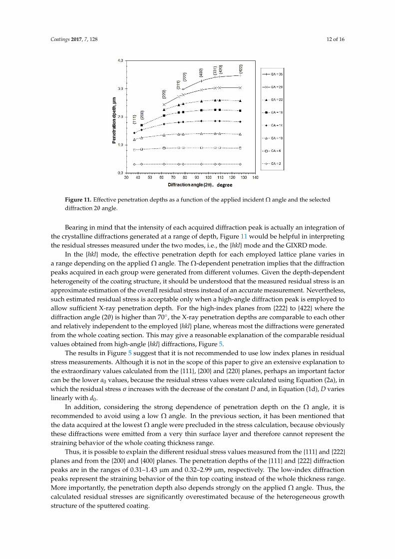
Figure 11. Effective penetration depths as a function of the applied incident Ω angle and the selected

diffraction 2θ angle.

Bearing in mind that the intensity of each acquired diffraction peak is actually an integration of

the crystalline diffractions generated at a range of depth, Figure 11 would be helpful in interpreting

the residual stresses measured under the two modes, i.e., the hkl mode and the GIXRD mode.

In the hkl mode, the effective penetration depth for each employed lattice plane varies in

a range depending on the applied Ω angle. The Ω-dependent penetration implies that the diffraction

peaks acquired in each group were generated from different volumes. Given the depth-dependent

heterogeneity of the coating structure, it should be understood that the measured residual stress is an

approximate estimation of the overall residual stress instead of an accurate measurement. Nevertheless,

such estimated residual stress is acceptable only when a high-angle diffraction peak is employed to

allow sufficient X-ray penetration depth. For the high-index planes from 222 to 422 where the

diffraction angle (2θ) is higher than 70, the X-ray penetration depths are comparable to each other

and relatively independent to the employed hkl plane, whereas most the diffractions were generated

from the whole coating section. This may give a reasonable explanation of the comparable residual

values obtained from high-angle hkl diffractions, Figure 5.

The results in Figure 5 suggest that it is not recommended to use low index planes in residual

stress measurements. Although it is not in the scope of this paper to give an extensive explanation to

the extraordinary values calculated from the 111, 200 and 220 planes, perhaps an important factor

can be the lower a0 values, because the residual stress values were calculated using Equation (2a), in

which the residual stress σ increases with the decrease of the constant D and, in Equation (1d), D varies

linearly with d0.

In addition, considering the strong dependence of penetration depth on the Ω angle, it is

recommended to avoid using a low Ω angle. In the previous section, it has been mentioned that

the data acquired at the lowest Ω angle were precluded in the stress calculation, because obviously

these diffractions were emitted from a very thin surface layer and therefore cannot represent the

straining behavior of the whole coating thickness range.

Thus, it is possible to explain the different residual stress values measured from the 111 and 222

planes and from the 200 and 400 planes. The penetration depths of the 111 and 222 diffraction

peaks are in the ranges of 0.31–1.43 µm and 0.32–2.99 µm, respectively. The low-index diffraction

peaks represent the straining behavior of the thin top coating instead of the whole thickness range.

More importantly, the penetration depth also depends strongly on the applied Ω angle. Thus, the

calculated residual stresses are significantly overestimated because of the heterogeneous growth

structure of the sputtered coating.

Coatings 2017, 7, 128 13 of 16

In the GIXRD mode, as shown in Figure 11, the X-ray penetration depth depends mainly

on the Ω angle regardless of the hkl plane. In other words, the diffraction peaks acquired at

each Ω angle were from the same depth, which is consistent with the analytical results of other

researchers [13–16]. Therefore, the calculated residual stress value each represents an integrated stress

value at certain coating thickness. Considering the fact that most hard coatings exhibit heterogeneous

structure depending on the plasma-assisted growth [16–21,26,28,29], the GIXRD mode has provided

an opportunity to analyze the depth profile of residual stresses, which also helps improve the

understanding of the heterogeneous structure.

At the lowest incident Ω angle of 2, the measured residual tensile stress and the substantially

smaller lattice parameter a0 are substantially different from those determined at higher Ω angles.

Because the intensity decreases quickly with increasing depth, the X-ray penetration was restrained in a

small depth of 0.3 µm. Therefore, the obtained diffractions should represent merely the crystallographic

property of the close vicinity of the coating surface. To the knowledge of the authors, there has been

no literature which addressed the unusual residual stresses experimentally measured in the extreme

surface layer of sputtered TiN coatings. Instead, the formation of tensile residual stresses in the initial

growth of thin films has been reported to be related to the constrained shrinkage when individual

islands begin to coalesce to each other [30–32]. It is known that the atomic stacking structure of the

as-grown coating surface differs greatly to the inner volume, seeing its roughness in atomic and nano

scales in Figure 2. In literature, it has been reported that a T-type sputtered coating exhibits dense

columnar grains and sub-dense grain boundaries, in which the atomic interaction forces between two

adjacent grains result in localized shrinkage and tensile residual stresses [33]. Such tensile stresses

at the grain boundaries are combined with the ion-peening induced compressive stresses inside the

dense grains to result in a decreased overall compressive residual stress [21,28]. These may partially

explain the different residual stresses as measured at the low incident Ω angle, whereas further detailed

explanation is beyond the scope of this paper.

When the Ω angle is higher than 10, the measured a0 values become more stabilized, which

may imply homogeneous nitrogen concentration of the TiN coating. The increased residual stress

with increasing Ω angle shows strong evidence of a stress profile along the depth direction. Because

the X-ray penetration depth depends almost only on the applied Ω angle and each diffraction peak

acquired at a certain Ω angle is actually the integration of diffractions of small volumes within a depth

defined by the Ω angle, it is needed to consider a method of analysis to determine a depth profile

of the actual residual stress, such as in literature [17–19]. Obviously, more extensive data processing

is required, which is beyond the focus of this paper. In brief, the GIXRD mode provides a valuable

analytical method to investigate the residual stress distribution in a heterogeneous coating system.

The residual stress can be expressed as a function of the applied Ω angle or X-ray penetration depth,

instead of a single value.

3.4. Effect of Anisotropic Elastic Modulus on the Calculated Residual Stress Values

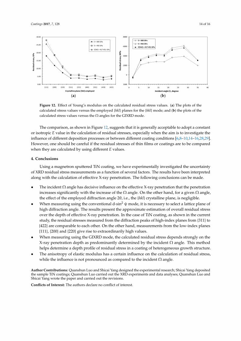
Figure 12 illustrates the effect of the adopted Young’s modulus values on the calculated residual

stresses both following the conventional hkl mode and the GIXRD mode. In Figure 12a, the residual

stress values are compared between the two adopted constant E values, namely, 456 GPa and 300 GPa.

Obviously, the higher E value leads to larger values of the calculated residual stress for its linear

relation to the elastic modulus, Equations (1) and (3). Similar relations are also obtained in the residual

stress values calculated out of the GIXRD mode, as shown in Figure 12b. For both measurement

modes, Figure 12a,b show limited influence of the anisotropic E values on the calculated residual stress

values. All the values are slightly lower than those obtained from the constant E value of 456 GPa,

but substantially higher than those from the E value of 300 GPa. These are not difficult to understand

as the adopted anisotropic E modulus, in the range of 417–451 GPa, are close to the higher constant

E value of 456 GPa.

Coatings 2017, 7, 128 14 of 16

(a) (b)

Figure 12. Effect of Young’s modulus on the calculated residual stress values. (a) The plots of the

‐

Ω ‐ Ω

Ω θ

‐ ψ ‐ ‐

‐

‐ Ω

Ω

‐ ‐

‐

‐30.00

‐25.00

‐20.00

‐15.00

‐10.00

‐5.00

0.00

111 200 220 311 222 400 331 420 422

Residual stress, G

Pa

Crystalline plane hkl employed

E = 300 GPa

E = 456 GPa

Ehkl = 417‐451 GPa

‐8000

‐6000

‐4000

‐2000

0

2000

0 5 10 15 20 25 30 35 40

Residual stress, M

Pa

Incident angle , degree

E = 300 GPa

E = 456 GPa

Ehkl = 417‐451 GPa

Figure 12. Effect of Young’s modulus on the calculated residual stress values. (a) The plots of the

calculated stress values versus the employed hkl planes for the hkl mode; and (b) the plots of the

calculated stress values versus the Ω angles for the GIXRD mode.

The comparison, as shown in Figure 12, suggests that it is generally acceptable to adopt a constant

or isotropic E value in the calculation of residual stresses, especially when the aim is to investigate the

influence of different deposition processes or between different coating conditions [6,8–10,14–16,28,29].

However, one should be careful if the residual stresses of thin films or coatings are to be compared

when they are calculated by using different E values.

4. Conclusions

Using a magnetron sputtered TiN coating, we have experimentally investigated the uncertainty

of XRD residual stress measurements as a function of several factors. The results have been interpreted

along with the calculation of effective X-ray penetration. The following conclusions can be made.

• The incident Ω angle has decisive influence on the effective X-ray penetration that the penetration

increases significantly with the increase of the Ω angle. On the other hand, for a given Ω angle,

the effect of the employed diffraction angle 2θ, i.e., the hkl crystalline plane, is negligible.

• When measuring using the conventional d-sin2 ψmode, it is necessary to select a lattice plane of

high diffraction angle. The results present the approximate estimation of overall residual stress

over the depth of effective X-ray penetration. In the case of TiN coating, as shown in the current

study, the residual stresses measured from the diffraction peaks of high-index planes from 311 to

422 are comparable to each other. On the other hand, measurements from the low-index planes

111, 200 and 220 give rise to extraordinarily high values.

• When measuring using the GIXRD mode, the calculated residual stress depends strongly on the

X-ray penetration depth as predominantly determined by the incident Ω angle. This method

helps determine a depth profile of residual stress in a coating of heterogeneous growth structure.

• The anisotropy of elastic modulus has a certain influence on the calculation of residual stress,

while the influence is not pronounced as compared to the incident Ω angle.

Author Contributions: Quanshun Luo and Shicai Yang designed the experimental research; Shicai Yang depositedthe sample TiN coatings; Quanshun Luo carried out the XRD experiments and data analyses; Quanshun Luo andShicai Yang wrote the paper and carried out the revisions.

Conflicts of Interest: The authors declare no conflict of interest.

Coatings 2017, 7, 128 15 of 16

References

1. Cullity, B.D.; Stock, S.R. Elements of X-ray Diffraction, 3rd ed.; Prentice Hall: Upper Saddle River, NJ, USA,

2001; p. 435.

2. Noyan, I.C.; Cohen, J.B. Residual Stress—Measurement by Diffraction and Interpretation; Springer: New York,

NY, USA, 1987; pp. 117–163.

3. Malhotra, S.G.; Rek, Z.U.; Yalisove, S.M.; Bilello, J.C. Analysis of thin film stress measurement techniques.

Thin Solid Films 1997, 301, 45–54. [CrossRef]

4. Fitzpatrick, M.E.; Fry, A.T.; Holdway, P.; Kandil, F.A.; Shackleton, J.; Suominen, L. Measurement Good Practice

Guide No. 52. Determination of Residual Stresses by X-ray Diffraction—Issue 2; National Physical Laboratory:

London, UK, 2006.

5. Portinha, A.; Teixeira, V.; Carneiro, J.; Beghi, M.G.; Bottani, C.E.; Franco, N.; Vassen, R.; Stoever, D.;

Sequeira, A.D.L. Residual stresses and elastic modulus of thermal barrier coatings graded in porosity.

Surf. Coat. Technol. 2004, 188–189, 120–128. [CrossRef]

6. Scardi, P.; Polonioli, P.; Ferrari, S. Residual stress in stabilized zirconia thin films prepared by RF magnetron

sputtering. Thin Solid Films 1994, 253, 349–355. [CrossRef]

7. Kim, J.O.; Achenbach, J.D.; Mirkarimi, P.B.; Shinn, M.; Barnett, S.A. Elastic constants of single-crystal

transition-metal nitride films measured by line-focus acoustic microscopy. J. Appl. Phys. 1992, 72, 1805–1811.

[CrossRef]

8. Perry, A.J.; Jagner, M.; Sproul, W.D.; Rudnik, P.J. The residual stress in TiN films deposited onto cemented

carbide by high-rate reactive sputtering. Surf. Coat. Technol. 1989, 39–40, 387–395. [CrossRef]

9. Quaeyhaegens, C.; Knuyt, G.; Stals, L.M. Study of the residual macroscopic stress in TiN coatings deposited

on various steel types (TuSA1). Surf. Coat. Technol. 1995, 74–75, 104–109. [CrossRef]

10. Liu, H.; Xu, Q.; Zhang, X.; Wang, C.; Tang, B. Residual stress analysis on TiN film fabricated by plasma

immersion ion implantation and deposition process. Nucl. Instrum. Methods Phys. Res. 2013, 297, 1–6.

[CrossRef]

11. Hohl, F.; Stock, H.-R.; Mayr, P. Examination of residual stress, morphology and mechanical properties of

sputtered TiN films. Surf. Coat. Technol. 1992, 54–55, 160–166. [CrossRef]

12. Saerens, A.; Houtte, P.V.; Meert, B.; Quaeyhaegens, C. Assessment of different X-ray stress measuring

techniques for thin titanium nitride coatings. J. Appl. Crystallogr. 2000, 33, 312–322. [CrossRef]

13. Welzel, U.; Ligot, J.; Lamparter, P.; Vermeulen, A.C.; Mittemeijer, E.J. Stress analysis of polycrystalline thin

films and surface regions by X-ray diffraction. J. Appl. Crystallogr. 2005, 38, 1–29. [CrossRef]

14. Benegra, M.; Lamas, D.G.; de Rapp, M.E.F.; Mingolo, N.; Kunrath, A.O.; Souza, R.M. Residual stresses in

titanium nitride thin films deposited by direct current and pulsed direct current unbalanced magnetron

sputtering. Thin Solid Films 2006, 494, 146–150. [CrossRef]

15. Skrzypek, S.J.; Baczmanski, A.; Ratuzek, W.; Kusior, E. New approach to stress analysis based on

grazing-incident X-ray diffraction. J. Appl. Crystallogr. 2001, 34, 427–435. [CrossRef]

16. Lewis, D.B.; Wadsworth, I.; Münz, W.D.; Kuzel, R., Jr.; Valvoda, V. Structure and stress of TiAlN/CrN

superlattice coatings as a function of CrN layer thickness. Surf. Coat. Technol. 1999, 116–119, 284–291. [CrossRef]

17. Genzel, C. X-ray stress analysis in presence of gradients and texture. Adv. X-ray Anal. 2001, 44, 247–257.

18. Marques, M.J.; Dias, A.M.; Gergaud, P.; Lebrun, J.L. A methodology development for the study of near

surface stress gradients. Mater. Sci. Eng. 2000, 287, 78–86. [CrossRef]

19. Jegou, S.; Christiansen, T.L.; Klaus, M.; Genzel, C.; Somers, M.A.J. Determination of composition,

residual stress and stacking fault depth profiles in expanded austenite with energy-dispersive diffraction.

Thin Solid Films 2013, 530, 71–76. [CrossRef]

20. Machunze, R.; Janssen, G.C.A.M. Stress and strain in titanium nitride thin films. Thin Solid Films 2009, 517,

5888–5893. [CrossRef]

21. Janssen, G.C.A.M.; Kamminga, J.D. Stress in hard metal films. Appl. Phys. Lett. 2004, 85, 3086–3088. [CrossRef]

22. Zhang, M.; He, J. Ab-initio calculation of elastic constants of TiN. Surf. Coat. Technol. 2001, 142–144, 125–131.

[CrossRef]

23. Sue, J.A. X-ray elastic-constants and residual-stress of textured titanium nitride coating. Surf. Coat. Technol.

1992, 54, 154–159. [CrossRef]

Coatings 2017, 7, 128 16 of 16

24. Abadias, G. Stress and preferred orientation in nitride-based PVD coatings. Surf. Coat. Technol. 2008, 202,

2223–2235. [CrossRef]

25. Luo, Q.; Jones, A.H. High-precision determination of residual stress of polycrystalline coatings using

optimised XRD-sin2ψ technique. Surf. Coat. Technol. 2010, 205, 1403–1408. [CrossRef]

26. Luo, Q.; Yang, S.; Cooke, K.E. Hybrid HIPIMS and CFUBMS deposition of TiN coatings: Deposition rate,

structure and tribological properties. Surf. Coat. Technol. 2013, 236, 13–21. [CrossRef]

27. Leeuwen, M.V.; Kamminga, J.D.; Mittemeijer, E.J. Diffraction stress analysis of thin films: Modeling and

experimental evaluation of elastic constants and grain interaction. J. Appl. Phys. 1999, 86, 1904–1915. [CrossRef]

28. Luo, Q.; Lewis, D.B.; Hovsepian, P.E.; Münz, W.-D. Transmission electron microscopy and X-ray diffraction

investigation of the microstructure of nano-scale multilayers TiAlN/VN grown by unbalanced magnetron

deposition. J. Mater. Res. 2004, 19, 1093–1104. [CrossRef]

29. Petrov, I.; Adibi, F.; Greene, J.E.; Hultman, L.; Sundgren, J.E. Average energy deposited per atom—A

universal parameter for described ion-assisted film growth. Appl. Phys. Lett. 1993, 63, 36–38. [CrossRef]

30. Hoffman, R.W. Stress in thin films: The relevance of grain boundaries and impurities. Thin Solid Films 1976,

34, 185–190. [CrossRef]

31. Nix, W.D.; Clemans, B.M. Crystallite coalescence: A mechanism for intrinsic tensile stresses in thin films.

J. Mater. Res. 1999, 14, 3467–3473. [CrossRef]

32. Freund, L.B.; Chason, E. Model for stress generated upon contact of neighbouring islands on the surface of

a substrate. J. Appl. Phys. 2001, 89, 4866–4873. [CrossRef]

33. Janssen, G.C.A.M. Critical review: Stress and strain in polycrystalline thin films. Thin Solid Films 2007, 515,

6654–6664. [CrossRef]

© 2017 by the authors. Licensee MDPI, Basel, Switzerland. This article is an open access

article distributed under the terms and conditions of the Creative Commons Attribution

(CC BY) license (http://creativecommons.org/licenses/by/4.0/).