Reproduced by

armed Services Technical nformation agency'DOCUMENT SERVICE CENTER

KNOTT BUILDING, DAYTON, 2, OHIO

UNCLA SSI-FIED

CV)

g ( j NATIONAL ADVISORY COMMITTEEF FOR AERONAUTICS

- TECHNICAL NOTE 2913

ON THE DEVELOPMENT OF TURBULENT WAKES

FROM VORTEX STREETS 1,, .

By Anatol Roshko

California Institute of Technology

Washington

March 1953

.4

1H NATIONAL ADVISORY COMMITTEE FOR AERONAUTICS

TECHNICAL NOTE 2913

ON THE DEVELOPMENT OF TURBULENT WAKES

FROM VORTEX STREETS

By Anatol Roshko

SUMMARY

Wake development behind circular cylinders at Reynolds numbers from40 to 10,000 was investigated in a low-speed wind tunnel. Standard hot-wire techniques were used to study the velocity fluctuations.

The Reynolds number range of periodic vortex shedding is dividedinto two distinct subranges. At R = 40 to 150, called the stable range,regular vortex streets are formed and no turbulent motion is developed.The range R = 150 to 300 is a transition range to a regime called theirregular range, in which turbulent velocity fluctuations accompany theperiodic formation of vortices. The turbulence is initiated by laminar-turbulent transition in the free layers which spring from the separationpoints on the cylinder. This transition first occurs in the rangeR = 150 to 300.

Spectrum and statistical measurements were made to study the velocityfluctuations. In the stable range the vortices decay by viscous diffusion.In the irregular range the diffusion is turbulent and the wake becomesfully turbulent in 40 to 50 diameters downstream.

It was found that in the stable range the vortex street has a periodicspanwise structure.

The dependence of shedding frequency on velocity was successfullyused to measure flow velocity.

Measurements in the wake of a ring showed that an annular vortexstreet is developed.

INTRODUCTION

It is always difficult to determine precisely the date and authorof a discovery or idea. This seems to be the case with the periodic

phenomena associated with flow about a cylinder. Although the effect

2 NACA TN 2913

of wind in producing vibrations in wires (aeolian tones) had been knownfor some time, the first experimental observations are due to Strouhal(reference 1) who showed that the frequency depends on the relative airvelocity and not the elastic properties of the wires. Soon after,Rayleigh (1879, references 2 and 3) performed similar experiments. Hisformulation of the Reynolds number dependence demonstrates his remarkableinsight into the problem.

These earliest observations were concerned with the relationsbetween vibration frequency and wind velocity. The periodic nature ofthe wake was discovered later, although Leonardo da Vinci in the fifteenthcentury had already drawn some rather accurate sketches of the vortexformation in the flow behind bluff bodies (reference 4). However,Leonardo's drawings show a symmetric row of vortices in the wake. Thefirst modern pictures showing the alternating arrangement of vorticesin the wake were published by Ahlborn in 1902 (reference 5); his visual-ization techniques have been used extensively since then. The importanceof this phenomenon, now known as the Kdrmnn vortex street, was pointedout by Benard (1908, reference 6).

In 1911 K~rmifu gave his famous theory of the vortex street (refer-ence 7), stimulating a widespread and lasting series of investigationsof the subject. For the most part these concerned themselves withexperimental comparisons of real vortex streets with Krmsn's idealizedmodel, calculations on the effects of various disturbances and configura-tions, and so on. It can hardly be said that any fundamental advance inthe problem has been made since KgrmAn's stability papers, in which healso clearly outlined the nature of the phenomenon and the unsolvedproblems. Outstanding perhaps is the problem of the periodic vortex-shedding mechanism, for which there is yet no suitable theoreticaltreatment.

However, the results of the many vortex-street studies, especiallythe experimental ones, are very useful for further progress in the prob-lem. Attention should be drawn to the work of Fage and his associates(1927, references 8 to 10), whose experimental investigations were con-ducted at Reynolds numbers well above the ranges examined by most otherinvestigators. Their measurements in the wake close behind a cylinderprovide much useful information about the nature of the shedding. Morerecently Kovasznay (1949, reference 11) has conducted a hot-wire inves-tigation of the stable vortex street (low Reynolds numbers), to whichfrequent reference will be made.

Vortex-street patterns which are stable and well-defined for longdistances downstream actually occur in only a small range of cylinderReynolds numbers, from about R = 40 to 150, and it is to this rangethat most of the attention has been given. On the other hand, as iswell-known, periodic vortex shedding also occurs at higher Reynolds

NACA TN 2913 3

numbers, up to 105 or more, but the free vortices which move downstreamare quickly obliterated, by turbulent diffusion, and a turbulent wakeis established.

The present interest in the vortex street is due to some questionsarising from the study of turbulent flow behind cylinders and grids.Such studies are usually made at Reynolds numbers for which periodicvortex shedding from the cylinders or grid rods might occur. However,the measurements are always taken downstream far enough to insure thatthe periodic velocity fluctuations are obliterated and the flow is com-pletely turbulent. There are several important consequences of thislimitation.

First, the energy of the velocity fluctuations is quite low comparedwith the energy near the cylinder, and especially low compared with thedissipation represented by the form drag. In attaining the developeddownstream state there is evidently not only a rapid redistribution ofenergy among the spectral components but also a large dissipation.Second, the theories which describe these downstream stages do not relatethe flow to the initial conditions except very loosely in terms ofdimensionless parameters, and it is usually necessary to determine anorigin empirically (e.g., mixing-length theory or similarity theories).

On the other hand, there is evidence that some features are perma-nent, so that they must be determined near the beginning of the motion.One such feature is the low-wave-number end of the spectrum which (inthe theory of homogeneous turbulence) is invariant.

Another is the random element. It has been pointed out by Dryden(references 12 and 13) that in the early stages of the decay of isotropicturbulence behind grids the bulk of the turbulent energy lies in aspectral range which is well approximated by the simple function

A characteristic of certain random processes. Liepmann (refer-1 + B2n2'ence 14) has suggested that such a random process may be found in theshedding of vortices fram the grids.

In short, there has been no description, other than very qualita-tive, of the downstream development of wakes which, over a wide rangeof Reynolds number, exhibit a definite periodicity at the beginning..The measurements reported here were undertaken to help bridge this gap.

The main results show the downstream development of the wake, interms of energy, spectrum, and statistical properties. This develop-ment is quite different in two Reynolds number ranges, the lower oneextending from about 40 to 150 and the upper, from 300 to 104 (and prob-ably 105), with a transition range between. The lower range is the

4 NACA TN 2913

region of the classic vortex street, stable and regular for a long dis-tance downstream. The fluctuating energy of the flow has a discretespectrum and simply decays downstream without transfer of energy toother frequencies. Irregular fluctuations are not developed. In theupper range there is still a predominant (shedding) frequency in thevelocity fluctuations near the cylinder, and most of the energy isconcentrated at this frequency; however, some irregularity is alreadydeveloped, and this corresponds to a continuous spectral distributionof some of the energy. Downstream, the discrete energy, at the sheddingfrequency, is quickly dissipated or transferred to other frequencies,so that by 50 diameters the wake is completely turbulent, and the energyspectrum of the velocity fluctuations approaches that of isotropicturbulence.

All other features of the periodic shedding and wake phenomena maybe classified as belonging to one or the other of the two ranges. Thisviewpoint allows some systematization in the study of wake development.

In particular, it is felt that the possibilities of the vortexstreet are by no means exhausted. A study of the interaction of periodicfluctuations with a turbulent field seems to be a fruitful approach tothe turbulence problem itself. It is planned to continue the presentwork along these lines.

From a more immediately practical viewpoint an understanding of theflow close to a bluff cylinder is important in at least two problems,namely, structural vibrations in members which themselves shed vorticesand structural buffeting experienced by members placed in the wakes ofbluff bodies. Many of these are most appropriately treated by the statis-tical methods developed in the theories of turbulence and other randomprocesses (reference 15). These methods are easily extended to includethe mixed turbulent-periodic phenomena associated with problems such asthe two mentioned above.

The research was conducted at GALCIT under the sponsorship and withthe financial assistance of the National Advisory Committee for Aeronautics,as part of a long-range turbulence study directed by Dr. H. W. Liepmann.His advice and interest throughout the investigation, as well as helpfuldiscussions with Dr. Paco Lagerstrom, are gratefully acknowledged.

SYMBOLS

A,B constants

a,b major and minor axis, respectively, of correlation ellipse

NACA TN 2913 5

CD drag coefficient

CDP form drag coefficient

D outside diameter of ring

d cylinder dimension

d' distance between free vortex layers

ds diameter of ring-supporting wire

E wake energy

E1 ,E2 components of wake energy due to periodic fluctuations

F dimensionless frequency nld2)

F(n) energy spectrum

Fl(n),F 2 (n) energy spectra of discrete energy

Fr(n) continuous energy spectrum

G(nA) output of wave analyzer at setting nA

h lateral spacing of vortices

h' initial lateral spacing of vortices

h* lateral spacing between positions of U'm

K constant

k integer

L scale

Lz scale corresponding to Rz

I downstream spacing of vortices

Mk moment, of order k, of probability density

6 NACA TN 2913

Nk "absolute" moment of probability density

nI shedding frequency

= 2n1

P() probability distribution function

p() probability density

Q area under response characteristic

q(r) tangential velocity in vortex

q* = q(r*)

R Reynolds number

R(n) response characteristic of wave analyzer

RD Reynolds number based on ring diameter

Rt(T) time correlation function

Rz () space correlation function

r distance from vortex center

r* radius of vortex

S Strouhal number, based on cylinder dimension (nld/Uo)

S' Strouhal number, based on distance between free vortexlayers (nld'/Uo)

T time scale

Ta time of averaging

t time

U local mean velocity in x-direction

Uo mean stream velocity

U* mean velocity at vortex center

NACA TN 2913 7

u,v,w components of velocity fluctuation

ul,u 2 periodic velocity fluctuations, at frequencies nI and n2

Ur random velocity fluctuation

u'm peak root-mean-square value of velocity fluctuation

V velocity of vortex relative to the fluid

x,y,z reference axes and distance from center of cylinder

flatness factor of probability distribution (MqM22

r strength (circulation) of a vortex

5(n) Dirac delta function

Epositive number

distance between two points, measured in z-direction

dimensionless frequency n)

e dimensionless "time" in life of vortex ( U )dummy variable

V kinematic viscosity

t a value of u

P density

a skewness of probability distribution (M3/ m2 3/2)

T time interval

CP dimensionless spectrum (U°FL ( n )

)half band width of wave analyzer

8 NAOCA TN 2913

GENERAL CONSIDERATIONS

Except for the parameters directly related to the shedding frequency,the quantities measured were essentially those that are standard inturbulence investigations (cf. references 12 to 14). These are brieflyreviewed below with some modifications required to study the periodicfeatures.

Reference Axes

The origin of axes is taken at the center of the cylinder (fig. 1);x is measured downstream in the direction of the free-stream velocity,z is measured along the axis of the cylinder, which is perpendicularto the free-stream velocity, and y is measured in the direction per-pendicular to (x,y); that is, y = 0 is the center plane of the wake.The free-stream velocity is Uo and the local mean velocity in thex-direction is U. The fluctuating velocities in the x, y, and zdirections are u, v, and w, respectively. The flow is consideredto be two-dimensional; that is, mean values are the same in all planesz = Constant.

Shedding Frequency

The shedding1 frequency is usually expressed in terms of the dimen-sionless Strouhal number S = nld/Uo, where n1 is the shedding fre-

quency (from one side of the cylinder), d is the cylinder diameter,and Uo is the free-stream velocity. The Strouhal number S may dependon Reynolds number, geometry, free-stream turbulence level, cylinderroughness, and so forth. The principal geometrical parameter is thecylinder shape (for other than circular cylinders, d is an appropriatedimension). However, cylinder-tunnel configurations must be taken intoaccount, for example, blockage and end effects. In water-channel experi-ments surface effects may have an influence. Usually the geometricalconfiguration is fixed, and then S is presented as a function ofReynolds number R.

Instead of Strouhal number it is sometimes convenient to use thedimensionless parameter F = nld2/v, where v is the kinematic viscosity.

1The term "shedding" is used throughout this report, for convenience;it is not meant to imply anything about the mechanism of the formation offree vortices.

NACA TN 2913 9

Energy

The experiments to be described are concerned mainly with thevelocity fluctuation in the wake, and especially with the correspondingenergy.

The energy of the velocity fluctuation at a point in the fluid is

* 2Ip(u2 + v2 + w2) per unit volume, where (u,v,w) is the fluctuating2velocity and the bar denotes an averaging (see the section "DistributionFunctions"). In these experiments only the component u was measured,and the term "energy" is used to denote the energy in that componentonly.

The energy intensity is defined as (u/Uo)2 . Since the mean flowis two-dimensional the intensity does not vary in the z-direction. Atany downstream position in the wake it varies in the y-direction, normalto the wake. The integral of the intensity over a plane normal to thefree stream (per unit span) is called the wake energy E:

E: U2dW W

The velocity fluctuation in the wake of a shedding cylinder displaysa predominant frequency (as well as harmonics) which is the sheddingfrequency. However, except in a small Reynolds number range, the fluctua-tion has random irregularities "superimposed" on it; that is, it is notpurely periodic, in the mathematical sense. However, it is convenientto speak of the "periodic" and "random" or turbulent parts of the

fluctuation.2 The energy may be written

u2 = u2 + u12 + u2

2 (2)

where ur2 is that portion of the energy contributed by the random

(turbulent) fluctuation, u12 is contributed by the periodic fluctua-

tion at the shedding frequency nl, and u22 corresponds to twice the

shedding frequency n2 = 2n1 . (The center of the wake feels the2A turbulent fluctuation is an irregular variation, with respect to

time, which is characterized in particular by its randomness and absenceof periodicity (cf. reference 13, p. 9).

10 NACA TN 2913

influence of vortices from both sides and n2 is prominent there, at

least near the "beginning" of the wake. Higher harmonics are found tobe negligible.)

Equation (2) is a kind of spectral resolution, in which u12 and

u22 are the energies at the specific frequencies nI and n2 . This

type of resolution is called a discrete, or line, spectrum. But

is not a discrete spectral component for it is the energy in the turbu-lent part of the fluctuation and contains "all" frequencies. It has acontinuous frequency distribution of energy, for which a slightly dif-ferent definition of spectrum is appropriate. This is postponed untilthe following section.

Corresponding to equation (2), an equation may be written for thewake energy E and its turbulent and periodic components:

E = Er + E1 + E2 (3)

Of particular interest will be the fraction of discrete energy(E 1 + E2)/E at various stages of wake development.

Correlation Functions; Spectrum

Definitions.- The time correlation function of the fluctuation u(t)is defined by

Rt(r) = u(t)u(t + T) (4)

where T is a time interval. The time scale is then defined by

T = I Rt d'r (5)

The Fourier transform of Rt defines another function

F(n) = 4 Rt(T) cos 2% nT dT (6)

NACA TN 2913 11

Then, also

Rt(r) = F(n) cos Zg nT dT (7)

For T = 0, equations (4) and(7) give

Rt(O) = F(n) dn 1 (8)

where F(n) is defined as the energy spectrum; that is, F(n) dn is thefraction of the energy in the frequency interval n to n + dn. It isthe fraction of energy "per unit frequency," as contrasted with the dis-crete energy spectrum discussed in the section "Energy."

In studies of isotropic turbulence, at Reynolds numbers corre-sponding to those in the present experiments, it is found that theenergy spectrum is well represented by the form

F(n) = 1+A B~2(9)

or, what amounts to the same thing, that the correlation function is ofthe form

Rt() = e-KT (10)

If the normalizing factor K = Uo/L is used in equation (10), L beinga characteristic length, then equation (6) gives

UOF(n) 4 (1a)

L 1 + 4.2(f2/Uo)

which may be conveniently written in terms of the dimensionless parameters

(= UoF(n)/L (12a)

and

= Ln (12b)U0

12 NACA TN 2913

Then

4 (11b)1 + (27t) 2

It is clear from equations (5) and (10) that L is a length scalerelated to the time scale by

L = UoT (13)

Equation (llb) is used as a convenient reference curve to comparethe measurements reported below.

Periodic functions.- The energy spectrum F(n) is particularlywell suited to turbulent fluctuations, for which the energy is con-tinuously distributed over the frequencies. For periodic fluctuationsthe discrete, or line, spectrum is more appropriate, but in the present"mixed" case it is convenient to write the discrete energy, also, interms of F(n). This may be done by using the Dirac delta function 8(n).Thus the energy at the shedding frequency nI is

Ul = Go B(n - nl) dn (14)

that is,

Fl(n) = 5(n - nl) (15)

Then the mixed turbulent-periodic fluctuations in the wake of a sheddingcylinder are considered to have an energy spectrum which is made up ofcontinuous and discrete parts (cf. equation (2) and appendix A):

U2 1 F(n) dn - U f Fr(n) dn + ul2 { Fl(n) dn +

u22- F2(n) dn (16)

that is,

) Ur" Fr(n) + Ul5(n - nl) +2 5(n - n2) (17)F U) uTu-

NACA TN 2913 13

Space correlation function; phase relations.- The correlation func-tion defined in equation (4) describes the time correlation. Anothercorrelation function which is useful in the present study is one whichrelates the velocity fluctuations at two points in the wake, situatedon a line parallel to the cylinder. This is defined by

Rz( ) = u(zt)u(z + ,t) (18)

u2

where is the distance between the two points. The correspondingscale is

Lz = Rz d (19)

The function Rz should be particularly suited to studying turbulentdevelopment. Close to the cylinder it should reflect the regularityconnected with the periodic shedding, especially in a regular, stablevortex street, in which there are no turbulent fluctuations. When thereare turbulent fluctuations and, especially, far downstream where thereis no more evidence of periodicity, Rz should be typical of a turbulentfluid; that is, the correlation should be small for large values of t.

The function Rz may be obtained by standard techniques applied tothe two signals u(z,t) and u(z + t,t). One well-known visual methodis to apply the signals to the vertical and horizontal plates, respec-tively, of an oscilloscope and to observe the resulting "correlationfigures" (or ellipses) on the screen (reference 16). If the signalsu(t) are turbulent fluctuations then the light spot moves irregularlyon the screen, forming a light patch which is elliptic in shape. Thecorrelation function is given by

= a2 - b2 (20)

a2 + b2

where a and b are the major and minor axes of the ellipse.

If u(z,t) is a periodic function, in both time and space, thenthe correlation figure is an elliptical loop (Lissajous figure) whosemajor and minor axes again give Rz according to equation (20). Sucha case would exist if the wake had a spanwise periodic structure. ThenRz(t) would be periodic. A special case of this is Rz(_) = 1, as wouldbe expected in a vortex street, provided the vortex filaments are straightand parallel to the cylinder and do not "wobble."

14 NACA TN 2913

Distribution Functions

Random functions.- The probability density p(k) of a randum func-tion ur(t) is defined as the probability of finding ur in the interval(Et + dt). It may be found by taking the average of observations madeon a large number (ensemble) of samples of ur(t), all these observationsbeing made at the same time t. This is called an ensemble average. IfUr(t) is a stationary process, as in the present case, then appeal ismade to the ergodic hypothesis and the ensemble average is replaced bythe time average, obtained by making a large number of observations ona single sample of ur(t). The probability density p(t) is the numberof times that ur is found in (, + dt) divided by the total number ofobservations made. In practice, time averages are more convenient thanensemble averages. The averaging time Ta must be large enough so thata statistically significant number of observations are made. This imposesno hardship; it is sufficient that Ta be large compared with the timescale T. If necessary, the error can be computed.

Experimentally, p(t) may be determined by the principle illustratedbelow: t V U t 2

"uk tn- t

t

- Tan

7- tip(g) Ti (21)

Ta

t i ILE (22)

Idur/dt I

The most elementary application of this principle is a graphical oneusing a photographic trace of ur(t). More conveniently, electroniccounting apparatus is employed (see the section "Statistical Analyzer").

The statistics of ur(t) are usually described in terms of themoments of p(g) and certain functions derived from the moments. The

NACA TN 2913 15

moment of order k is defined as

Mk = gp) dt (23)

Another useful definition is

Nk =f 00 jkp(t) dt (24)

where Nk is equal to M k for even values of k. If p(t) issymmetrical, then M k is 0 for odd values of k but Nk is not.

From the definition of p(k) it follows that M0 = p(t) dt = 1;

will be normalized by requiring that M2 = 1/2, that is, the mean-square value ur 2 = 1/2.

Three useful functions derived from the moments are

21/ - /N1 (25)

Skewness a= Y (26)

Flatness = M4 (27)

Periodic functions.- The above definitions may be extended to thecase of a periodic function ul(t). The probability density can becompletely determined from a single wave length of ul(t); that is, itis sufficient to take Ta equal to the period. This complete a prioriinformation is a basic difference between periodic and random functions. 3

3For a periodic function the ergodic principle may not be invoked;the ensemble average and the time average are not the same (unless themembers of the ensemble have random phase differences). It is the timeaverage that is computed here, for comparison with the experimentalresults, which are also time averages.

1

16 NACA TN 2913

If ul(t) is measured experimentally then ti(t) in equation (21)can also be measured. If ul(t) is given in analytic form then ti(t)may be calculated from equation (22). Thus the distribution densitiesfor simple wave shapes are easily calculated. Table I gives the prob-ability densities and moments for the triangular wave, sine wave, andsquare wave. Also included is the Gaussian probability density, whichis a standard reference for random functions.

The moments of the probability densities of these wave shapes areshown in figure 2. The moments for the random function increase muchfaster than those for the periodic functions. This results from thefact that the maximum values of a periodic function are fixed by itsamplitude, while for a random function all values are possible.

The probability density of a function which is partly periodic andpartly random is expected to display the transition from one type to theother. The tendency toward the random probability density should bestrong. For instance, random fluctuations in the amplitude of a sinewave result in a large increase in the higher moments. It is interestingto study the relation between probability functions and spectra, partic-ularly the case where most of the energy is discrete but the fluctua-tion amplitude is random.

EXPERIMENTAL DATA

Wind Tunnel

The experiments were all made in the GALCIT 20- by 20-inch low-turbulence tunnel (fig. 1). The turbulence level is about 0.03 percent.The wind velocity may be varied from about 50 centimeters per second(1 mph) to 1200 centimeters per second (25 mph).

Cylinders

The cylinders used in the experiments varied in diameter from0.0235 to 0.635 centimeter. Music wire or drill rod was used. Thediameter tolerances are about 0.0002 centimeter. The cylinders spannedthe tunnel so that the length in all cases was 50 centimeters (20 in.);the cylinders passed through the walls and were fastened outside thetunnel.

3H NACA TN 2913 17

Rings

Some studies were made of the flow behind rings. These were madeup of wire. Each ring was supported in the tunnel by three thin supportwires, attached to the ring circumference at 1200 intervals. Table IIgives the dimensions of the rings used (where d is the wire diameter,D, the ring diameter, and ds, the diameter of the support wire).

Velocity Measurements

Velocities higher than about 400 centimeters per second weremeasured with a pitot tube, calibrated against a standard. The pres-sures were read on a precision manometer to an accuracy of about0.002 centimeter of alcohol. Velocities lower than 400 centimeters persecond were determined from the shedding frequency of a. reference cylinder(0.635 cm), as explained in the section "Use of Shedding Frequency forVelocity Measurements."

Fluctuating velocities were measured with a hot-wire anemometer(1/20 mil platinum). Only u(t), the fluctuating velocity in the flow

direction, has been measured so far. The hot-wire was always parallelto the cylinder.

Traversing Mechanism

The hot-wire was mounted on a micrometer head which allowed it tobe traversed normal to the wake and positioned to 0.001 centimeter.The head was mounted on a horizontal lead screw which allowed traversingin the flow direction, in the center plane of the tunnel. The posi-tionng in this direction was accurate to about 0.01 centimeter. Thehorizontal lead screw could be turned through 900 to allow traversingparallel to the cylinder, for correlation or phase measurements (section"Space correlation function; phase relations"). For this purpose, asecond micrometer head with hot-wire could be set up in a fixed positionalong the line of traverse of the first hot-wire. Then correlationscould be measured between this point and the movable one.

Electronic Equipment

The hot-wire output was amplified by an amplifier provided withcompensation up to 10,000 cycles per second. The amplifier output couldbe observed on an oscilloscope screen or measured on a Hewlett-Packard

Model 400c vacuum-tube voltmeter. Values of u2 were obtained by readingthe root-mean-square voltage on the voltmeter. (This voltmeter isactually an average-reading meter; it reads true root-mean-square values

18 NACA TN 2913

only for a sine wave. A few of the indicated root-mean-square values,for turbulent velocity fluctuations, were checked against true root-mean-square values as obtained from the statistical analyzer (see thesection "Statistical Analyzer"); these may differ up to 10 percent,depending on the wave shape, but, at present, no corrections have beenmade, since the absolute values were not of prime interest.) Usually

only relative values of u2 were required, but absolute values couldbe determined by comparing the voltage with that obtained by placingthe hot-wire behind a calibrated grid.

The frequencies of periodic fluctuations were determined byobserving Lissajous figures on the oscilloscope; that is, the amplifieroutput was placed on one set of plates and a known frequency on theother. This reference frequency was taken from a Hewlett-Packard Model202B audio oscillator, which supplied a frequency within 2 percent ofthat indicated on the dial.

Frequency Analyzer

Spectra were measured on a Hewlett-Packard Model 300A harmonicwave analyzer. This analyzer has an adjustable band width from 30 to145 cycles per second (defined in appendix A) and a frequency rangefrom 0 to 16,000 cycles. The output was computed directly from readingsof the voltmeter on the analyzer. It was not felt practicable to readoutput in the frequency range below 40 cycles; therefore, the continuousspectrum was extrapolated to zero frequency.

To determine the discrete spectrum in the presence of a continuousbackground some care was required. In such cases the analyzer readinggives the sum of the discrete spectral energy and a portion of that inthe continuous spectrum, the proportions being determined by the responsecharacteristic of the wave analyzer. The value in the continuous partwas determined by interpolation between bands adjacent to the discreteband and subtracted'out to give the discrete value, as outlined in moredetail in appendix A.

Statistical Analyzer

The statistical analyzer, designed to obtain probability functions,operates on the principle described in the section "Distribution Functions;"here u(t) is a voltage signal. A pulse train (fig. 3) is modulated byu(t) and is then fed into a discriminator which "fires" only when theinput pulses exceed a certain bias setting, that is, only when u(t) > E.For each such input pulse the discriminator output is a pulse of constantamplitude. The pulses from the discriminator are counted by a series ofelectronic decade counters terminating in a mechanical counter.

NACA TN 2913 19

The complete analyzer consists of 10 such discriminator-counterchannels, each adjusted to count above a different value of E. It willbe seen that the probability function obtained is the integral of theprobability density described in the section "Distribution Functions;"that is,

P()= Probability that u(t) >

t p p(p) d1±

It is possible to rewrite the moments (section "Distribution Functions")in terms of p(), a more convenient form for calculation with thisanalyzer. These are also shown in table I.

More complete details of the analyzer and computation methods maybe found in references 17 and 18.

RESULTS

Shedding Frequency

Since Strouhal's first measurements in 1878 (reference 1) therelation between the shedding frequency and the velocity has been ofinterest to many investigators. Rayleigh (reference 2, p. 413) pointedout that the parameter nld/Uo (now called the Strouhal number S) shouldbe a function of the Reynolds number. Since then there have been manymeasurements of the relationship (reference 19, p. 570). One of thelatest of these is the measurement by Kovasznay (reference 11), whosedetermination of S(R) covers the range of R from 0 to l04. Kovasznayalso made detailed investigations of the vortex-street flow pattern atlow Reynolds numbers. He observed that the street is developed only atReynolds numbers above 40 and that it is stable and regular only atReynolds numbers below about 160.

The present measurements of S(R) are given in figures 4 and 5.Except at Reynolds numbers between 150 and 300, the scatter is small,and the measurements agree with those of Kovasznay. The large numberof cylinder sizes used results in overlapping ranges of velocity andfrequency so that errors in their measurement should be "smeared" out.It is believed that the best-fit line is accurate to 1 percent.

The measurements are corrected for tunnel blockage but no attemptis made to account for end effects. With the cylinder sizes used nosystematic variations were detected.

20 NACA TN 2913

Nature of Velocity Fluctuations

It was observed, as in Kovasznay's work, that a stable, regularvortex street is obtained only in the Reynolds number range from about40 to 150. The velocity fluctuations in this range, as detected by ahot-wire, are shown on the oscillograms in figure 6, for a Reynoldsnumber of 80. These were taken at two downstream positions, x/d = 6and 48, and at several values of y/d. (The relative amplitudes arecorrect at each value of x/d, but the oscillograms for x/d = 48 areto a larger scale than those for x/d = 6.) The frequencies and ampli-tudes are quite steady; it is quite easy to determine the frequenciesfrom Lissajous figures (section "Electronic Equipment"), which, of course,are also steady.

Another example, at R = 145, is shown in figure 7(a). (The doublesignal was obtained for correlation studies and is referred to later inthe section "Spanwise Correlation and Phase Measurements." The dottednature of the trace is due to the method of obtaining two signals on onescreen, using an electronic switch.)

At Reynolds numbers between about 150 and 300 there are irregularbursts in the signal. An example is shown in figure 7(b), at R = 180and x/d = 6. The bursts and irregularities become more violent as Rincreases. It is rather difficult to determine the frequency. TheLissajous figure is unsteady because of the irregularity, but, in addi-tion, the frequency, as well as it can be determined, varies a little.This is the reason for the scatter in this Reynolds number range. Twoseparate plots of S(R) obtained in two different runs are shown infigure 8. They illustrate the erratic behavior of S(R) in this range.

At Reynolds numbers above 300, signals like that in figure 7(c)were obtained (near the beginning of the wake). This is typical of thevelocity fluctuations up to the highest value of R investigated (about10,000). There are irregularities, but the predominant (shedding)frequency is easy to determine from a Lissajous figure. The Lissajousfigure in this case is not a steady loop, as it is at R = 40 to 150,but neither is it so capricious as that at R = 150 to 300, and thematching frequency is quite easily distinguished from the nearbyfrequencies.

At x/d = 48, in this range, all traces of the periodicity havedisappeared and the fluctuations are typically turbulent.

Regular and Irregular Vortex Streets

The above observations show that there are three characteristicReynolds number ranges, within the lower end of the shedding range.

NACA TN 2913 21

These will be called as follows:

Stable range 40 < R < 150

Transition range 150 < R < 300

Irregular range 300 < R < 10,000+

As noted above, the actual limits of these ranges are somewhat in doubtand may depend on configuration, free-stream turbulence, and so forth.Also the upper limit of the irregular range is undoubtedly higher than10,000. (Periodic fluctuations in the wake have been observed up tothe critical Reynolds number, about 200,000, but the present measurementsdid not extend beyond 10,000.)

In addition to the differences in the nature of the velocity fluc-tuations, the ranges are characterized by the behavior of the Strouhalnumber: In the stable range S(R) is rapidly rising, in the irregularrange it is essentially constant, and in the transition range it is"unstable."

It will be seen in the further results presented below that allphases of the wake development are different in the two ranges, stableand irregular, and that they are indeed two different regimes of peri-odic wake phenomena.

Relation of Shedding Frequency to Drag

The relation between the Strouhal number S(R) and the drag coef-ficient CD (R) has often been noted (reference 19, p. 421). Roughly,rising values of S(R) are accompanied by falling values of CD(R)and vice versa.

The relation to the form drag is even more interesting. The totaldrag of a cylinder is the sum of two contributions: The skin frictionand the normal pressure. At Reynolds numbers in the shedding range theskin-friction drag is "dissipated" mainly in the cylinder boundary layer,while the pressure drag (or form drag) is dissipated in the wake. Itmay, then, be more significant to relate the shedding frequency to theform drag, both of which are separation phenomena. The R-dependence ofthe pressure drag coefficient CDp, taken from reference 19, page 425,is shown in figure 5. It has several interesting features:

(a) CDP is practically constant, at the value CDp = 1.

(b) The minimum point A is at a value of R close to that at whichvortex shedding starts.

22 NACA TN 2913

(c) The maximum point B is in the transition range.

(d) In the irregular range CDp(R) is almost a "mirror reflection"of S(R).

Since the drag coefficient is an "integrated" phenomenon, it isnot expected to display so sharply detailed a dependence on R as does

the Strouhal number, but these analogous variations are believed to beclosely related to the position of the boundary-layer separation point,to which both the shedding frequency and the pressure drag are quitesensitive.

Use of Shedding Frequency for Velocity Measurements

The remarkable dependence of the shedding frequency on the velocityand the possibility of accurately measuring S(R) make it possible todetermine flow velocities from frequency measurements in the wake of acylinder immersed in the flow. At normal velocities the accuracy is asgood as that obtainable with a conventional manometer, while at veloc-ities below about 400 centimeters per second it is much better. (Forinstance, at a velocity of 50 cm/sec the manometer reading is only about0.001 cm of alcohol.) In fact, in determining S(R) in the presentexperiments, this method was used to measure the low velocities bymeasuring the shedding frequency at a second reference cylinder of largediameter. The self-consistency of this method and the agreement withKovasznay's results are shown in figure 4.

For velocity measurements it is convenient to plot the frequency-velocity relation in terms of the dimensionless parameter F (see thesection "Shedding Frequency") as has been done in figures 9 and 10.The points on these plots were taken from the best-fit line in figure 4.They are well fitted by straight lines

(la) F = 0.212R - 4.5 50 < R < 150

(1b) F = 0.212R - 2.7 300 < R < 2000

which correspond to

(2a) S = 0.212(1 - 21.2/R) 50 < R < 150

(2b) S = 0.212(1 - 12.7/R) 300 < R < 2000

Line (2b) has been plotted in figure 4 to compare with what is consideredthe best-fit line. The agreement is better than 1 percent. If line (2b)is extended up to R = 10,000, the maximum error, relative to the best-fit line, is 4 percent.

NACA TN 2913 23

The plot of F(R) is used as follows: The shedding frequency is

observed and F = nld2/v is calculated (v is easily determined); R isfound on the F(R) plot and the velocity is calculated from R = Uod/V.Sometimes, as in the present experiments, only R is required.

Wake Energy

From the velocity traces on the oscilloscope (figs. 6 and 7) it isclear that in the regular range the fluctuating velocity u(t) is purelyperiodic while in the irregular range some of the fluctuations are random.This difference is illustrated in figure 11 which shows the distribution

of energy intensity (u/Uo)2 across the wake at two Reynolds numbers, onein the regular range, at R = 150, and one in the irregular range, atR = 500. Only half the wake is shown for each case; the one at R = 150is plotted on the left side of the figure and the one for R = 500, onthe right.

The total energy intensity (u/Uo)2 at each point was determineddirectly from the reading on the root-mean-square voltmeter (see thesection "Electronic Equipment"). The components at the frequencies n1and n2 were determined by passing the signal through the wave analyzer.The curves in each half of figure 11 satisfy the equalities

(o2 = () + (u2)1 R = 150

() = (u) + + (u)2 R = 500

The values of (u/Uo) 2, (ul/Uo)2, and (uZ/Uo)2 were obtained by

measurement (and at R = 150 are self-consistent) while (ur/Uo)2 wasobtained by difference. The absolute values indicated are somewhat indoubt since the vacuum-tube voltmeter is not a true root-mean-squaremeter but are believed accurate to about 10 percent.

The particular feature illustrated in figure 11 (already obviousfrom the oscillographs) is the absence of turbulent energy at R = 150as contrasted with the early appearance of turbulent energy at R = 500.This contrast is typical of the regular and irregular ranges.

24 NACA TN 2913

The measurements shown were made at 6 diameters downstream, butthe same features exist closer to the cylinder. In fact, fluctuationsin the flow can be detected ahead of the cylinder. They display thetypical characteristics in the two ranges.

Downstream Wake Development

The downstream development for the case of figure 11 (but R = 500

only) is shown in figure 12. The distribution of total energy intensity

(u/Uo)2 is shown on the left of the figure and the discrete energy

intensity (ul/Uo)2, at the shedding frequency, is shown on the right.Traverses were made at 6, 12, 24, and 48 diameters downstream. Thediscrete energy decays quite rapidly and is no longer measurable at

48 diameters. (Note that the plot of (Ul/Uo) 2 at 24 diam is shown

magnified 10 times, for clarity.) A plot of (u2/Uo)2 has not beenincluded since it can no longer be measured at even 12 diameters. The

distribution of (ur/Uo)2 may be obtained from these curves by difference.

Figure 13 presents the downstream wake development in another way.The wake energy E was calculated by integration of curves like thosein figure 12 (cf. the section "Energy"); that is,

E = f7.2 dt(y)

Figure 13 is a plot of the energy ratio (El + E2)/E, that is, the ratioof the discrete energy relative to the total energy.

In the irregular range the energies were computed in this way atR = 500 and 4000 (two cylinder sizes in each case) and R = 2900 (onecylinder). Figure 13 shows that the decay in all these cases is similarand the wake is completely turbulent at 40 to 50 diameters.

The value of x/d for which El/E becomes zero was determinedfor a variety of cylinders, varying in size from 0.06 to 1.3 centimetersand at Reynolds numbers from 200 to 10,000. The value was found to liebetween 40 and 50 in all cases but closer to 40. A precise determina-tion is difficult (and not important) because of the asymptotic approachof El/E to zero (E2 is already zero at less than 12 diam).

In contrast with this, the stable range (R = 50 and 100 in fig. 13)has no development of turbulence before 50 diameters. The plots forR = 150 and 200 illustrate the rather spectacular transition from thestable range to the irregular.

4H NACA TN 2913 25

For R = 50 and 100 the energy ratio remained constant at unity upto x/d = 100. Beyond that the energy intensity is so low that the tunnelturbulence cannot be neglected.

Measurements of Spectrum

Figure 14 shows spectrum measurements at 6, 12, 24., and 48 diametersdownstream at a Reynolds number of 500, in the irregular range. Thelateral position y/d chosen for the measurement at each x/d is the

one for which (ul/Uo)2 is a maximum (cf. fig. 12). The method ofplotting is as follows. The curve through the experimental points isthe continuous spectrum Fr(n), plotted in normalized coordinates. Thediscrete energies F1 = 5(n - nl) and F2 = 5(n - n2 ) are indicated

by narrow "bands" which should have zero width and infinite height butare left "open" in the figure. The relative energies represented bythe areas under the continuous curve and under the delta functions, respec-

tively, are marked in the figure with values of ur2/u2 and ul2/u 2 ,

u22/u2 .

To normalize the continuous spectrum the dimensionless parameters

cp=oFr~n) and L n are used. In each case the curveL 4 U0

1 + (2~~ )2 is included for reference. The normalizing coefficient L

was determined as follows:

(a) Fr(O) was found by extrapolation of the measured values to

n = 0.

(b) Fr(0) and the other values of Fr(n) were normalized to make

j F(n) dn = 1.

(c) L was found from -.° Fr(O) = 4.L

In short, the measured curve and the reference curve were made to agreein Tr(0) and in area. This requirement determines L.

In these coordinates the shedding frequency shows an apparentincrease downstream; this is because the normalizing parameter Lincreases. For x/d = 48 the shedding frequency (i.e., nl) is markedwith a dash; it contains no discrete energy at this value of x/d.

26 NACA TN 2913

The "bumps" in the continuous spectrum, near n1 and n2, indicatea feeding of energy from the discrete to the continuous spectrum. Theportion of the spectrum near n = 0, which is established early and whichcontains a large part of the turbulent energy, seems to be unrelated tothe shedding frequency (cf. fig. 15). As the wake develops the energyin the bumps is rapidly redistributed (part of it decays) to smooth thespectrum, which, in the fully developed turbulent wake at 48 diameters,

4tends toward the characteristic curve q =

L + (2)

In figure 16 the spectrum for x/d = 12 and y/d = 0.8 is plottedtogether with the one at y/d = 0. The curves are similar at low fre-quencies (large eddies) and at high frequencies; they differ only inthe neighborhood of the discrete band. (The slight discrepancy betweenthis figure and fig. 14 is due to the fact that they were measured attwo different times, when the kinematic viscosity v differed. Thisresulted in different values of n1 at the same R.)

A similar downstream development is shown in figure 15 for R = 4000.Here the spectrum at x/d = 6 is smoother than that in the previousexample (fig. 14). This effect may be due not so much to the higherReynolds number as to the fact that the shedding frequency is closer tothe low frequencies; that is, the shedding frequency is "embedded" inthe low-frequency turbulent band. It seems to result, at 48 diameters,in a much closer approach to the reference curve.

Figure 17 shows the spectra at 48 diameters for three cylinders andseveral values of y/d. It is remarkable that R = 4000, d = 0.477 cmagrees better with R = 500, d = 0.190 cm than with R = 4000,d = 0.953 cm. This seems to bear out the above remark about the rela-tive influence of R and nl, for the respective shedding frequenciesare 565, 440, and 144.

Finally it may be noted that values of ur2, which in figure 11were obtained by difference, check well with the values computed from

Ur2 = Fr(n) dn (before normalization of Fr(n)).

Spectra for the regular range are not presented, for they are simplediscrete spectra.

NACA TN 2913 27

Spanwise Correlation and Phase Measurements

The function Rz was not measured, but the main features of thespanwise correlation4 are illustrated in figures 7 and 18.

Figure 7 shows three examples, in each of which simultaneous signalswere obtained from two hot-wires at x/d = 6 and y/d = 1 and separatedby 50 diameters ppanwise. The two signals were obtained simultaneouslyon the oscilloscope screen by means of an electronic switch. Thisaccounts for the dotted traces.

At R = 145 (fig. 7(a)) the correlation is perfect but there is aphase shift. At R = 180 (fig. 7(b)) the correlation is still good butthe individual signals occasionally break down. The breakdowns areuncorrelated at this distance of 50 diameters. At R = 500 (fig. 7(c))each signal still shows a predominant frequency. There is some variationin phase between the two signals. The amplitude irregularities appearto be uncorrelated.

Figure 18 shows the correlation figures obtained by placing thesignals of the two hot-wires on the horizontal and vertical plates,respectively, of the oscilloscope.

For R = 80 and t/d = 100 a steady Lissajous figure is obtained,showing that the periodic fluctuations at the two points (100 diam apart)are perfectly correlated (.but they are not in phase).

For R = 220 and 500 there is good correlation only at small valuesof t/d, that is, only when the two hot-wires are in the same "eddy," soto speak. For R = 500 the figures are similar to those obtained infully developed turbulence.

In obtaining these correlations a remarkable phenomenon was observed.The stable vortex street (that is, R < 150) has a periodic spanwisestructure. This was shown by the phase shifts on the Lissajous figure,as the movable hot-wire was traversed parallel to the cylinder. Fromthe phase coincidences observed, the wave length parallel to the cylinderwas about 18 diameters at a Reynolds number of 80. It has not been deter-mined whether this periodicity structure is due to a "waviness" in thevortex filaments or whether the vortex filaments are straight but inclinedto the cylinder axis.

41n the remainder of this section a distinction is made between theterms "correlation function" and "correlation." The former refers tothe function defined in the section "Space correlation function; phaserelations" while the latter is used in a looser, descriptive sense.

28 NACA TN 2913

Statistical Measurements

A few amplitude distribution functions were measured and are shownin figure 19. One measurement is in the stable range; the other showsdownstream development in the irregular range.

The table in figure 19 shows values of c and a computed fromthese curves. The behavior, of course, is as expected, but the numericalvalues are of some interest. These values (and the curves) show that atR = 100 the signal was practically triangular but had rounded "tops,"At R = 500 the downstream development of randomness is shown by thetendency of c and m toward the Gaussian values.

The distribution is in fact not Gaussian, as may be seen in thefigure, for its skewness a is quite high.

Vortex Rings

The flow behind wire rings was briefly investigated. The dimensionsof the rings used are given in table II.

With the rings of diameter ratio D/d = 10 vortices are shed fromthe wire in almost the same way as from the straight wire, and there isapparently an annular vortex street for some distance downstream. TheStrouhal number, measured from R = 70 to 500, is lower than that forthe straight wire (about 3 percent at R = 500 and 6 percent at R = 100).

Fluctuating velocity amplitudes were measured in the wake at severaldownstream positions. The results for the largest ring, measured along a

diameter, are shown in figure 20. It should be noted that CU ratherthan the energy has been plotted here (cf. fig. 11); only relative val-ues were computed. Close behind the cylinder the wake behind the wireon each side of the ring is similar to that behind the straight wire,but the inside peaks are lower than the outside peaks. This may bepartly due to the interference of the hot-wire probe, for a similareffect, much less pronounced, was noticed in the measurements behind astraight wire.

Farther downstream there was some indication of strong interactionbetween the vortices, for a peak could not be followed "smoothly" down-stream. However, the investigations were not continued far enough toreach conclusive results. At about 40 diameters downstream the flowbecame unstable.

NACA TN 2913 29

The ring with D/d = 5 behaved somewhat differently. The observedfrequencies gave values of Strouhal number as shown in table III. Thetable shows values of S and R based on the wire diameter, as wellas values of SD and RD based on ring diameter. Between R = 153and 182 there is a sudden increase in S, and at higher Reynolds numbers,in what corresponds to the irregular range, the shedding is similar tothat from a straight wire, while in the stable range the shedding is ata much lower frequency. From the observations made it seems likely thatin the stable range the ring acts like a disk, shedding the vortex loopsobserved by Stanton and Marshall (reference 18, p. 578, and reference 20).Stanton and Marshal do not give their frequency-velocity observationsexcept at the critical RD, where shedding first starts. They observedthis to be at about RD = 200, with a corresponding SD of 0.12.

Again, these experiments were too incomplete to warrant definiteconclusions, but the difference in behavior for D/d = 10 and D/d = 5is interesting. This behavior is similar to that observed by Spivack(reference 21) in his investigation of the frequencies in the wake of apair of cylinders which were separated, normal to the flow, by a gap.He found that when the gap was just smaller than 1 diameter instabilityoccurred. For larger gaps the cylinders behaved like individual bodies,while for smaller gaps the main frequencies were, roughly, those corre-sponding to a single bluff body of dimension equal to that of the combinedpair, including the gap.

DISCUSSION

The most significant results of this investigation may be discussedin terms of the Reynolds number ranges defined in the section "Regularand Irregular Vortex Streets," namely, the stable range from R = 40 to 150,the transition range from R = 150 to 300, and the irregular range aboveR = 300.

Stability

The transition range from R = 150 to 300 displays the character-istics of a laminar-turbulent transition, and it is instructive to comparethe stability of the flow around the cylinder with boundary-layer sta-bility. The flow in the irregular range has turbulent characteristics,while in the stable range it is essentially viscous.

The Reynolds number regimes may be described as follows: BelowR = 40 the flow around the cylinder is a symmetric, viscous configura-tion, with a pair of standing vortices behind the cylinder. At aboutR = 40 this symnetric configuration becomes unstable. It changes to a

30 NACA TN 2913

new, stable configuration which consists of alternate periodic breakingaway of the vortices and formation of a regular vortex street. Theinstability at R = 40 is not a laminar-turbulent instability; itdivides two different ranges of stable, viscous flow. In either range,disturbances to the stable configuration will be damped out.

On the other hand, the transition range from R = 150 to 300involves a laminar-turbulent transition. To understand how this transi-tion is related to the vortex shedding, it is necessary to know somethingabout the formation of the vortices. Involved in this formation is thecirculating motion behind the cylinder as shown in the following sketch.A free vortex layer (the separated boundary layer) springs from eachseparation point on the cylinder. This free layer and the backflow behindthe cylinder establish a circulation from which fluid "breaks away" atregular intervals.

rTurbulentShear layer 1 minar

The laminar-turbulent transition is believed to occur always inthe free vortex layer; that is, the circulating fluid becomes turbulentbefore it breaks away. Then each vortex passing downstream is composedof turbulent fluid.

The point in the free vortex layer at which the transition occurswill depend on the Reynolds number. This transition was actually observedby Schiller and Linke (reference 18, p. 555, and reference 22) whosemeasurements were made at cylinder Reynolds numbers from 3500 to 8500.The distance to the transition point, measured from the separation point,decreased from 1.4 diameters to 0.7 diameter, and for a given Reynoldsnumber these distances decreased when the free-stream turbulence wasincreased. Dryden (reference 23) observed that at some value of R,depending on free-stream turbulence and so forth, the transition pointin the layer actually reaches the separation point on the cylinder.This point then remains fixed and vortex shedding continues, essentiallyunchanged, up to Reynolds numbers above 100,000, that is, up to thevalue of R for which transition begins in the cylinder boundary layerahead of the separation point. It is quite likely that even above this

NACA TN 2913 31

critical value of R the phenomenon is essentially unchanged, but nowthe vortex layers are much nearer together and the vortices are diffusedin a much shorter downstream distance.

In summary, vortex formation in the stable range occurs withoutlaminar-turbulent transition. The circulating fluid breaks away peri-odically, and alternately from the two sides, forming free "viscous"vortices which move downstream and arrange themselves in the familiarvortex street. In the irregular range transition occurs in the circu-lating fluid before it breaks away, and the vortices are composed ofturbulent fluid. The transition range corresponds to the similar rangein boundary-layer stability, and it displays a similar intermittency.The values R = 150 and 300 used to define the range are expected tobe different in other experiments, depending on wind-tunnel turbulence,cylinder roughness, and so forth.

Shedding Frequency

The Strouhal number and Reynolds number dependence is different inthe two ranges. In the stable range S(R) is rapidly rising, while inthe irregular range it is practically constant.

Fage and Johansen, who investigated the structure of the free vortexlayers springing from the separation points on various bluff cylinders(reference 9), made an interesting observation on the relation of theshedding frequency to the distance between the vortex layers. Thisdistance increases as the cylinder becomes more bluff, while the sheddingfrequency decreases. In fact, if a new Strouhal number S' is definedin terms of the distance d' between the free vortex layers (insteadof the cylinder dimension d), then a universal value S' - 0.28 isobtained for a variety of (bluff) cylinder shapes. The measurements ofreference 9 were made at R = 20,000, but it is believed that the simi-larity exists over the whole irregular range. It does not extend to thestable range. To check this point the shedding frequency was measuredin the wake of a half cylinder placed with the flat face broadside tothe flow. It was found that S(R) was rising for Reynolds numbers below300 and then became practically constant at the value S = 0.140. For asimilar case, at R = 20,000, Fage and Johansen found S = 0.143.

The universality of the constant S' is useful in systematizingthe shedding phenomena (at least in the irregular range). It indicatesthat when the circulating fluid behind the cylinder is turbulent thenthe formation of free vortices is similar for a variety of bluff shapesand over a wide range of Reynolds numbers.

Finally, the relation between Strouhal number and form drag coef-ficient has been mentioned in the section "Relation of Shedding Frequency

to Drag." In the irregular range the slight variations in S(R) reflectslight variations of CDp and so, probably, of the separation point.

32 NACA TN 2913

However, constancy of CDp is not enough to insure a fixed separation

point. For instance, CDp remains practically constant down to Reynolds

numbers below the shedding range, but the separation point there isfarther back than it is at higher Reynolds numbers. It would seem worthwhile, and fairly easy, to measure the position of separation as a func-tion of Reynolds number over the whole shedding range, that is, to com-plete the data available in the literature.

Downstream Development

The way in which the wake develops downstream is quite differentin the stable and irregular ranges.

When the circulating fluid breaks away before the occurrence oftransition in the free vortex layers (i.e., below R = 150) then thefree vortices which are formed are the typical viscous vortices. Thereis no further possibility for the fluid in them to become turbulent.The vortices simply decay by viscous diffusion as they move downstream(see the section "Spread of Vortex Street" in appendix B).

When turbulent transition does occur, then the vortices which areformed consist of turbulent fluid. They diffuse rapidly as they movedownstream and are soon obliterated, so that no evidence of the sheddingfrequency remains. This development to a completely turbulent wake takesplace in less than 50 diameters. In terms of the decay of the discreteenergy (fig. 13), the development is roughly the same for Reynolds numbersfrom 300 to 10,000. This again indicates a remarkable similarity overthe whole irregular range.

The stable and irregular ranges are also characterized by the dif-ference in the energy spectra of the velocity fluctuations. It has beenpointed out that in the irregular range a continuous, or turbulent, partof the spectrum is established at the beginning of the wake development.This turbulence is a result of the transition in the free vortex layersand might be expected to be independent (at first) of the periodic partof the fluctuation, which results from the periodic shedding. Indeed,most of the energy at first is concentrated at the shedding frequency n,(some at n2), and it may be represented as a discrete (delta function)part of the spectrum, within the accuracy of the measurements (cf.appendix A). However, the continuous and discrete parts are not entirelyindependent, as shown by the bumps near nI and n2 (fig. 14). Thismay be regarded as a result of energy "feeding" from the discrete to thecontinuous parts of the spectrum, and it proceeds in a way which tendsto smooth the spectrum. Such transfer of energy between spectral bandsis a process depending on the nonlinear terms of the equations of motion.The "activity" in the spectrum, at any stage of its development, may be

5H NACA TN 2913 33

regarded as an equilibrium between the nonlinear and the viscous terms.It is an important problem in the theory of isotropic turbulence.

The spectral activity near the frequency of discrete energy mightbe looked upon as a simplified case in which a single band has an excessof energy and the spectral energy flow is unidirectional, that is, outof it into the adjacent bands. However, the nonhomogeneous character ofthe field involved (the wake) reduces the simplicity, for it is necessaryto take account of energy transfer across the wake. One interestingpossibility is to superimpose a homogeneous (isotropic) turbulent field,by means of a screen ahead of the shedding cylinder, and to study theeffect of this field on the spectral activity near the discrete band.Although the wake will still introduce nonhomogeneity (not even countingthe periodic part of the motion), it may be possible to arrange therelative magnitudes to give significant results from the simplified model.

To study such problems the technique for measuring the spectrum(appendix A) near the frequency of discrete energy will be improved.

To summarize, it is suggested that the initial development of thespectrum might be regarded as follows. The continuous and the discreteparts are established independently, the one by the transition in thevortex layers and the other by the periodic shedding. The turbulencedue to the transition is the "primary" turbulent field and its spectrumis the typical, continuous (turbulent) spectrum. (It has been noted inthe section "Measurements of Spectrum" that the low-frequency end of thespectrum is established early; it would contain only energy of the primaryfield.5 ) The discrete part of the spectrum is embedded in the turbulentpart, and it thereby is "excited" into spectral transfer. Some of itsenergy is transferred to the adjacent frequency bands resulting, initially,in the development of bumps in the continuous spectrum. Subsequently, asthe spectral transfer proceeds, the spectrum becomes smooth.

The above discussion is an abstract way of saying that the vorticesare diffused by a turbulent fluid (instead of a viscous one). The dif-fusion involves the nonlinear processes typical of turbulence; the studyof these processes, in terms of spectrum, is an important problem.

There is a similar case of turbulent, periodic structure in theflow field between two cylinders, one of which rotates. Taylor's dis-covery of the periodic structure of the flow is well-known (reference 24).When the inner cylinder rotates, it is possible to obtain a steady, regular

51n the theory of homogeneous turbulence it is shown that the low-frequency end of the spectrum is invariant, a property related to theLoitsianski invariant.

3NACA TN 2913

arrangement of ring vortices, enclosing the inner cylinder, and having,alternately, opposite directions of circulation. Above a critical valueof the speed of rotation this laminar, periodic structure becomes unstableand the fluid becomes turbulent, but alternate ring-shaped vortices stillexist at speeds several hundred times the critical speed (reference 25).

Statistics

The probability distribution functions (fig. 19) display thecharacteristics which are expected, from the other observations. Thecontrast between the functions at R = 100 and R = 500, that is, inthe stable and irregular ranges, respectively, is quite evident. Inthe irregular range, even at x/d = 6, where most of the energy isdiscrete, there is a marked irregularity in the fluctuation, as shownby the high value of m.

However, these descriptions are little better than qualitative, andit is hoped to obtain more interesting results by extending these sta-tistical methods. Of particular interest in the development of randomfrom periodic motion would be the relation between the probability dis-tributions and the spectra. For instance, it is plain that a purelyperiodic function (discrete spectrum) will have a probability distribu-tion with finite cutoff, while development of random irregularities inthe function's amplitude is strongly reflected in (1) a "spreading" ofthe distribution function to higher values of t and (2) the appearanceof a continuous spectrum. However, the relation between the two is notunique; that is, the spectrum does not give (complete) information aboutthe probability distribution, and vice versa. It is not clear what thecorrespondence is and whether useful relationships nay be obtained, pos-sibly for restricted classes of functions.

Suggestions for Future Investigations

Some further lines of investigation indicated by these experimentsare summarized below.

(a) The transition from the stable to the irregular range shouldbe investigated with controlled disturbances, for example, cylinderroughness and free-stream turbulence. It is expected that the limitsof the transition range (roughly R = 150 to 300 for the experimentalconditions here) will be lower for higher free-stream turbulence orcylinder roughness. The critical cylinder Reynolds numbers should berelated to corresponding numbers for the transition point in the freevortex layers (based on distance from separation point or on the thick-ness of the layer).

NACA TN 2913 35

Such studies of stability to different disturbance amplitudes andfrequencies are well-known in the case of the boundary layer. A varia-tion of the experiments of Schubauer and Skramstad (reference 26), whoused an oscillating wire in the boundary layer to produce disturbancesof definite frequencies, would be to use a second shedding cylinder.

(b) A study of the spectral development in the neighborhood of adiscrete band, the effect of a turbulent field on its activity, and soforth (discussed in the section "Downstream Development") may be the mostfruitful continuation of these experiments. So far, the problem has beenapproached only in the theory of isotropic turbulence, where it has notadvanced much beyond the similarity considerations of Kolmogoroff, andvery little is known about the form of the spectral transfer function.

Interactions between discrete bands, for example, at slightly dif-ferent frequencies, can be studied by the use of two or more cylindersarranged to "interfere" with each other (some such studies have beenmade by Spivack (reference 21) but not from this viewpoint), or possiblyby using one cylinder having diameter changes along its span.

(c) Townsend has recently used the concepts of intermittentlyturbulent flow and local isotropy in his investigations of the turbulentwake and has obtained a new description of its structure (reference 27).His studies were made at downstream distances of 80 diameters or more,so that the wake was fully turbulent. Probably the structure he describesis essentially the same up to the beginning of the fully developed wake(about 50 diam), but then there is the question of how it is related tothe earlier developments. The most obvious "early developments" are theturbulent transition in the free vortex layers and the periodic shedding.(Although the shedding frequency is no longer distinguished far down-stream, it is prominent in the early spectral developments and thus hasan influence on the downstream wake.)

Such studies will involve considerably more detailed investigations

of the wake structure than were made here, possibly along the lines ofTownsend's experiments and the classical measurements of energy balance

across the wake. The other two components of the energy v2 and w2

will be needed.

(d) The nature of the circulating flow behind the cylinder and theformation of free vortices, that is, the shedding mechanism, shouldreceive further attention.

(e) The spanwise periodic structure of the vortex street shouldbe investigated, beyond the very cursory observations made here. Inparticular, a study of the stability of single vortex filaments seemsimportant.

36 NACA TN 2913

(f) Measurements of the fluctuating forces on the cylinder, dueto the shedding, would be interesting and should have immediate practicalapplications. There seems to be very little information about the magni-tude of these forces. It might be obtained either by direct measurementof forces (on a segment) or pressures (with pressure pickups) or inferredfrom measurements of the velocity fluctuations close to the cylinder. Inaddition to the magnitude of the force or pressure fluctuations, theirspanwise correlation is of prime importance.

CONCLUSIONS

An experimental investigation of the wake developed behind circularcylinders at Reynolds numbers from 40 to 10,000 indicated the followingconclusions:

1. Periodic wake phenomena behind bluff cylinders may be classifiedinto two distinct Reynolds number ranges (joined by a transition range).For a circular cylinder these are:

Stable range 40 < R < 150

Transition range 150 < R < 300

Irregular range 300 < R < 10,000+

In the stable range the classical, stable KErm6n streets are formed;in the irregular range the periodic shedding is accompanied by irregular,or turbulent, velocity fluctuations.

2. The irregular velocity fluctuation is initiated by a laminar-turbulent transition in the free vortex layers which spring from theseparation points on the cylinder. The first turbulent bursts occurin the transition range defined above.

3. In the stable range the free vortices, which move downstream,decay by viscous diffusion, and no turbulent motion is developed. Inthe irregular range the free vortices contain turbulent fluid and diffusefaster; the wake becomes fully turbulent in 40 to 50 diameters.

4. A velocity meter based on the relation between velocity andshedding frequency is practical.

5. In the stable range a spanwise periodic structure of the vortexstreet has been observed.

NACA TN 2913 37

6. An annular vortex-street structure has been observed behind ringshaving a diameter ratio as low as 10.

California Institute of Technology

Pasadena, Calif., May 29, 1952

38 NACA TN 2913

APPENDIX A

EXPERIMENTAL ANALYSIS OF SPECTRUM

These notes supplement the brief descriptions in the sections"Frequency Analyzer" and "Measurements of Spectrum."

Analyzer Response

Consider the response of a spectrum analyzer, such as that used inthe present experiments, to a mixed periodic-random input, and in particu-lar consider the problem of inferring the input from the output.

The input, an energy or power, has a random and a periodic component:

U2=U2+U2 (Al)u- =u + u1

The corresponding spectra are defined by

= u2 F(n) dn

= U Fr(n) dn (A2)

7-2-u WfF(n) dn= Ul2 l n

where

Fl(n) = B(n - nl) (A3)

and 5(n) is the Dirac delta function.

The response characteristic of the analyzer may be obtained by

considering the effect of a periodic input. When the analyzer settingnA coincides with the input frequency n1 the output is a maximum,

NACA TN 2913 39

and when the setting is moved away from nI the output falls off. Theresponse characteristic is

Output at setting nAR(nl - nA) = =at setting nA = R(nA - nl ) (A)

Output a etn A=n

The output spectrum G(nA) of the analyzer is related to the inputspectrum F(n) by (cf. reference 15)

G(nA) = F(n)R(n - nA) dn

- r(n)R(n- nA) dn + u12 bO(nl - nA)R(n - hA) dn

Ur2 r.wFr(n)R(n - nA) dn + u- R(nI - nA) (A5)

UfJ U2

Since R(n - nA) is sharp, that is, almost a delta function (see thesection "Half Band Width," Fr(n) may be considered to be constant overthe significant interval of integration in equation (A5). Then

G(nA) = - Fr(nA)Q + U R(nI - nA) (M)u2 u2

where

Q = R(n - nA) dn= R(n - nA) dnA (A7)

is the area under the response characteristic.

Equation (A6) gives the output for a mixed periodic-random input.It is required to find the separate terms which make up this sum. Theprocedure is outlined in the section "Separation of Discrete Energy" below.

40 NACA TN 2913

Half Band Width

The resolution of the analyzer is determined by its half bandwidth w. This is defined as the number of "cycles off resonance" atwhich the output falls off to 0.01 percent; that is

R(n 1 - W) = 0.0001 (A8)

For an ideal analyzer the response characteristic would be a deltafunction, but even with half band widths from 30 to 145 (which is therange of the analyzer used here) the characteristic is quite sharp, rela-tive to the frequency intervals of interest. The values 30 to 145 seemquite high, but they are a little misleading because of the high attenua-tion used to define w. For example, if the response-characteristichalf band width c is 30 cycles per second it has a total width of only6 cycles per second at 50 percent attenuation.

Separation of Discrete Energy

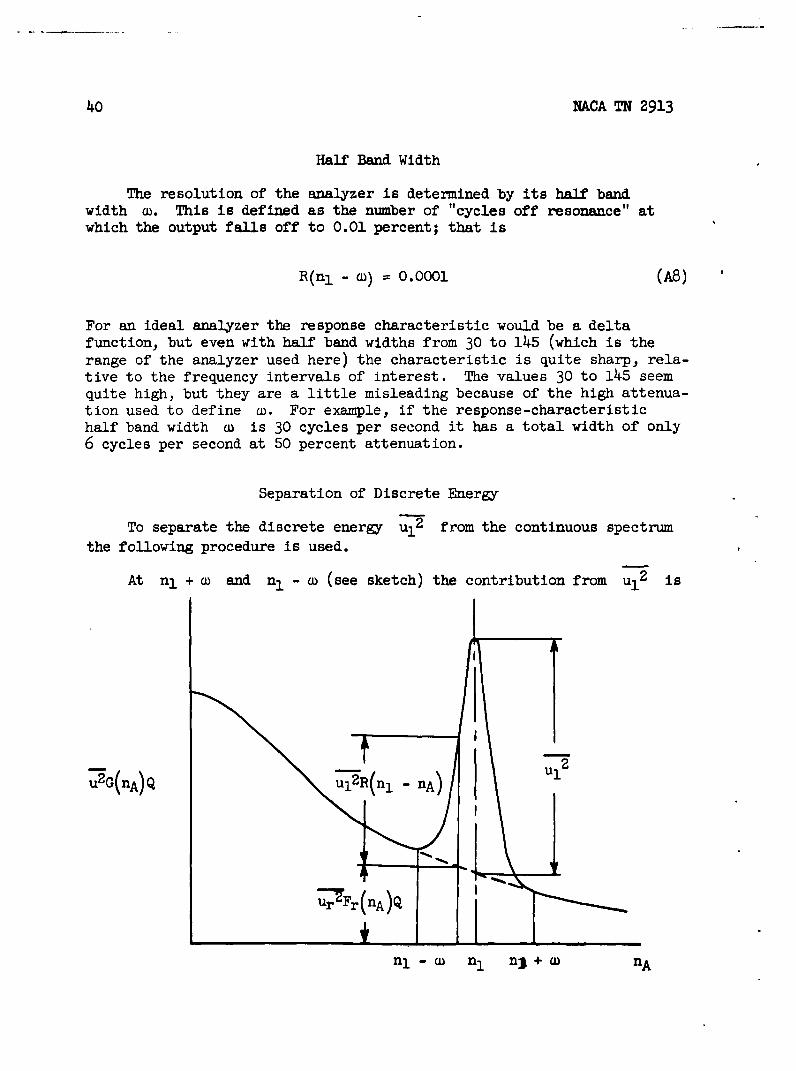
To separate the discrete energy ul2 from the continuous spectrumthe following procedure is used.

At nI + w and nI - w (see sketch) the contribution from ul2 is

u2G(nA)Q -u1 2Rjj 2 A) U1

urnFr (nA) Q

nl-co n, n3 + w

6H NACA TN 2913 41

only 0.01 percent, so the measured points there are assumed to lie on thecontinuous spectrum. It is assumed at first that the continuous spectrumbetween these points may be determined by interpolation, and its value

at nI is calculated. Then u12 is determined by difference and the

last term in equation (A7) is calculated, since the form R(n) is known.The first term in equation (A6) then gives the values of G(nA) in thevicinity of nl; these should check the measured values.

If, however, the continuous spectrum within the band width has abump, then the above calculation is not self-consistent, and the true

values can be determined by successive estimates of U12 .

In principle the method is satisfactory, but in practice theaccuracy is low because in the regions of interest, that is, near peakfrequencies, it depends on the differences of relatively large quantities.One of these, R(n), is known precisely, but the precision is difficultto realize since the settings on the analyzer cannot be read accuratelyenough. For the spectral investigations discussed in the section"Downstream Development" the technique will be improved.

42 NACA TN 2913

APPENDIX B

NOTES ON VORTEX-STREET GEOMETRY AND SHEDDING FREQUENCY

The regularity of the vortex shedding and its sensitivity tovelocity changes have undoubtedly intrigued everyone who has investigatedthe flow past bluff bodies. However, as K~rm n pointed out in his firstpapers on the vortex street, the problem is inherently difficult,involving as it does the separation of the boundary layer from thecylinder, and there is yet no adequate theoretical treatment of themechanism.

The following notes may be useful as a summary of the interestingfeatures of the problem. They are based largely on the literature butinclude some results obtained during the present experiments. Chapter XIIIof reference 19 has a very useful review and list of references.

Idealized K~rmkn Street

Ka i' s theory treats a double row of potential vortices, infinitein both directions. The distance between the rows h and the spacingof the vortices in each row I are constants. The vortices have strength(circulation) P which, with the geometry, determines the velocity Vof the street relative to the fluid. The theory shows that the configura-tion is stable when the rows are staggered by a half wave length and thespacing ratio is

h = 0.281 (Bl)

The circulation and velocity relative to the fluid are then related by

- = 2.83 (B2)V1

Two of the parameters (h, 1, r, and V) must be determined from someother considerations. In the real vortex street they must be relatedto the conditions at the cylinder.

Real Vortex Street

The real vortex street, even in the stable range, differs from theidealized one in the following points:

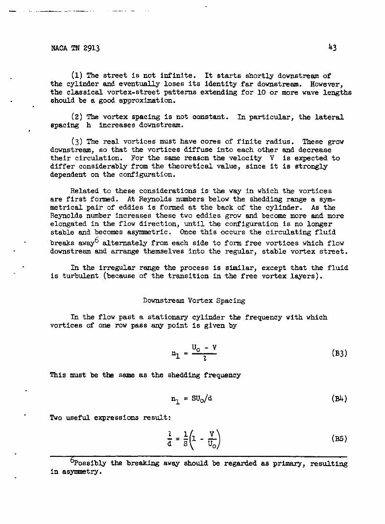
NACA TN 2913

(1) The street is not infinite. It starts shortly downstream ofthe cylinder and eventually loses its identity far downstream. However,the classical vortex-street patterns extending for 10 or more wave lengthsshould be a good approximation.

(2) The vortex spacing is not oonstant. In particular, the lateralspacing h increases downstream.

(3) The real vortices must have cores of finite radius. These growdownstream, so that the vortices diffuse into each other and decreasetheir circulation. For the same reason the velocity V is expected todiffer considerably from the theoretical value, since it is stronglydependent on the configuration.

Related to these considerations is the way in which the vorticesare first formed. At Reynolds numbers below the shedding range a sym-metrical pair of eddies is formed at the back of the cylinder. As theReynolds number increases these two eddies grow and become more and moreelongated in the flow direction, until the configuration is no longerstable and becomes asymmetric. Once this occurs the circulating fluid

breaks away6 alternately from each side to form free vortices which flowdownstream and arrange themselves into the regular, stable vortex street.

In the irregular range the process is similar, except that the fluidis turbulent (because of the transition in the free vortex layers).

Downstream Vortex Spacing

In the flow past a stationary cylinder the frequency with whichvortices of one row pass any point is given by

n u - _O (B3)

This must be the same as the shedding frequency

n= SUo/d (B4)

Two useful expressions result:

1= - - U-)(B5)

6 possibly the breaking away should be regarded as primary, resulting

in asymmetry.

44 NACA TN 2913

or

V= SZ (B6)U T

Z 1In a real vortex street, V -3-o far downstream and then --.. Or,

if SI/d is known from measurements, then V/Uo may be computed.

An example of measured values of 1/d is shown in figure 21. Thesewere taken from the streamline plot obtained by Kovasznay (reference 11)at R = 53 (for which S = 0.128). There is a little scatter but 1/ddoes approach the constant value 1/S = 7.8.

The scatter, while relatively unimportant in the case of I/d,gives very low accuracy for values of V/Uo calculated from equation (B6).These have also been plotted in figure 21. It is surprising that someof the values, near the cylinder, are negative (corresponding to valuesof 1/d higher than l/S); it is believed that this results frum thecombined difficulty of estimating the vortex centers, especially nearthe cylinder, and the sensitivity of equation (B6). (However, it mustbe noted that negative values of V are not impossible. Negative Vsimply means that the vortex velocity is directed upstream relative tothe fluid, while it is still downstream relative to the cylinder. Sucha possibility exists at low values of x/d, where the mean velocity atthe edges of the wake is considerably higher than Uo.)

Another way to obtain V/Uo is to assume that the vortex centersmove with the local mean velocity. Kovasznay's paper includes measure-ments of mean velocity profiles. From his results the mean velocityalong the line of vortex centers U* has been determined and from it

= I U* has been calculated. The result is plotted in figure 21.

Near the cylinder it does not agree with the values obtained by theprevious method; it is believed that this is principally due to thedifficulties mentioned above and that the determination of V/Uo from1 - (U*/Uo) i; more accurate.

Lateral Spacing

The lateral spacing, at least initially, must be determined byconditions near the cylinder. The way in which this spacing increasesdownstream is discussed, for the stable range, in the section "Spreadof Vortex Street."

NACA TN 2913 45

In the irregular range, the dependence of the shedding frequencyon the distance between the free vortex layers, noted by Fage and Johansen(see the section "Shedding Frequency"), leads to an interesting estimateof the initial lateral spacing of the free vortices. The maximum dis-tance d' between the free vortex layers, instead of the cylinder dimen-sion d, may be used to define a new Strouhal number

d'

S= n1 d'_ (B7)

Fage and Johansen found that, whereas S varies considerably withcylinder shape, S' is practically constant for a variety of bluffcylinders. Now the initial lateral spacing h' of the free vorticeswill be roughly the same as d', possibly a little smaller:

hl = (1 - E)dl (B)

Then, comparing with equations (B6) and (B7),

T 1 (v/uo)

From the measurements of Fage and Johansen, S' 0.28. The factor

1 - 1 E 1. Thus equation (B9) gives h'/1 = 0.28; that is, the

1 - (V/Uo)

spacing ratio agrees with KdrmAn's value, at least close to the cylinder.

Shedding Frequency

There is yet no adequate theory of the periodic vortex shedding,and it is not clear what is the principal mechanism which determinesthe frequency.

The downstream spacing ratio is related to the shedding frequencyby equation (B3) and to the lateral spacing by a stability criterion(e.g., Kdrm~n's value of 0.28 for the idealized street). It might beconsidered that the shedding frequency is determined by the spacingrequirement, or, conversely, that the shedding is primary and determinesthe downstream spacing. The latter viewpoint seems the more plausibleone; that is, the shedding frequency is established by a mechanism whichdepends on features other than the vortex spacing. It is necessary to

46 NACA TN 2913

obtain a better understanding of the flow field near the cylinder. Oneof the elements involves the problem of separation, particularly thenonstationary problem. Another that requires more study is the flowfield directly behind the cylinder.

With a better knowledge of these, and possibly other, features itmay be possible to set up a model of the shedding mechanism. In themeantime it is not clear whether the vortex spacing requirement isdecisive in determining the frequency.

Destabilization7 of Shedding

The following experiment illustrates the dependence of the periodicshedding on "communication" between the free vortex layers, that is, onthe flow field directly behind the cylinder. A thin flat plate wasmounted behind the cylinder in the center plane of the wake (fig. 22).It was completely effective in stopping the periodic shedding. Spectrummeasurements in the flow on one side of the plate are shown in figure 22.At R = 7500 no significant frequencies could be separated out from thecontinuous background. At R = 3200 there were several predominantfrequencies (all higher than the shedding frequency for the cylinder),but, by the time the flow reached the end of the plate, 5 diametersdownstream, it was completely turbulent. (The shedding frequency n,for the cylinder is marked in the figures.)

The important effect, on the shedding, of the flow field directlybehind the cylinder is apparent. Probably an even shorter length ofplate would be effective in destabilizing the periodic shedding, andthere may be a most effective position for such an interference element.Kovasznay remarks that the hot-wire probe used in investigating thevortex street must be inserted from the side, for if it lies in theplane of the street it has a strong destabilizing influence.

A more complete study of the destabilization of shedding by suchinterference devices may be quite useful from a practical viewpoint.Structural vibrations and failures are often attributed to the periodicforces set up on members exposed to wind or other flow (smokestacks,pipe lines, structural columns, to mention a few). In many cases itmight be possible to destabilize the vortex shedd..ing by addition ofsimple interference elements or by incorporating them in the originaldesigns. In the case where one member is buffeted by the wake of anotherthe same principle might be applied.

7The stability considered in this section is not with respect tolaminar-turbulent transition; it concerns the stability of the periodicshedding (cf. the section "Stability").

NACA TN 2913 47

Spread of Vortex Street

It has been observed by most investigators that the spacing ratioh/ is KArmAn's value (0.28) close to the cylinder but increases rapidlydownstream. The increase of h/1 is mainly due to the increase of h,since I changes very little (fig. 21). In the stable range this isthe result of viscous diffusion of the real vortices.

Hooker (reference 28) has made an interesting analysis. First, areal vortex has a core of finite radius; its center is the point of zerovelocity and maximum vorticity. Hooker shows that in a vortex street,where the velocity field of the other vortices must be taken into account,the points of zero velocity and maximum vorticity do not coincide. Thepoint of maximum vorticity is unchanged but the point of zero velocityis farther away from the center of the street. As the vortex decays,the point of zero velocity moves farther out, its distance from thecenter of the street increasing almost linearly with time. Thus thespacing based on vorticity centers remains constant, while the spacingbased on velocity centers increases linearly. Hooker's calculation ofthe linear spread checks fairly well with some pictures taken by Richards(reference 29) in the wake of an elliptical cylinder having a finenessratio of 6:1 and the major diameter parallel to the free-stream velocity.

However, the spread of the wake is not always observed to be linear.Among the different investigators there is a large variation of results,apparently dependent on the experimental arrangement. In Richards'experiment the cylinder was towed in a water tank and the vortex patternswere observed on the free surface.

In Kovasznay's experiment the cylinder was mounted in a wind tunnel,the arrangement being similar to the one used here (see the section"Experimental Data"). On his plot of the streamlines at R = 53 thedownstream spread of the vortex street is parabolic rather than linear.It is possible to fit his results by a somewhat different applicationof Hooker's idea, using decaying vortex filaments.

Each vortex in the street is considered to behave like a singlevortex filament carried along by the fluid, its decay or diffusion beingthe same as if it were at rest. The decay of such a vortex is describedby a heat equation, whose solution is (reference 30, p. 592):

q = r - e - r 2 1 vt) (Blo)

where q is the tangential velocity at the distance r from the centerand at the time t. The circulation is P. This is essentially a vortexwith a "solid" core and potential outer flow joined by a transition

48 NACA TN 2913

region in which the velocity has a maximim value. This maximum velocityis

= 0.72(r/2nr*) (BIU)

and occurs at the radial distancd

r* = 2.24(vt)1/2 (Bl2)

Here r* is defined as the vortex radius.

Thus the radius increases as tl/2 and the maximum velocity decreases

as t - 1 / 2 . In the vortex street, the time t is replaced by the downstreamdistance x. Since the vortices move with the velocity U* rather than

U0, the dimensionless time e = U0 X is appropriate, where U* alsoU* d

varies downstream (see the section "Downstream Vortex Spacing").

When a pattern of such vortices is superimposed on a uniform flow,it is possible to calculate the velocity fluctuation at a point, becauseof the pattern passing over it.

Now the following hypothesis is added. It is assumed that thevortex radius r* is equal to the width h of the street. Then the

width of the street increases as xl/2.

A second result follows. The maximum velocity fluctuation (observedby a hot-wire, say) will occur on the line of vortex centers and will havethe amplitude

u* 1 q* (B13)

that is, the hot-wire encounters instantaneous velocities varying fromU* (because of vortex centers passing over it) to U* + q* (due to thefields of vortices on the other side of the street). Relations (Bll)and (B12) then give the downstream behavior of the maximum fluctuationamplitude.

The results may be summarized as follows:

(a) Wake width h el/2.

(b) The maximum amplitude of fluctuation u* occurs on the lineof vortex centers (so there are two maximum points across the wake).

NACA TN 2913 49

(c) u* ze-ll 2 .

(d) u* = 0.36(r12 h).

A comparison of the above predictions was made with calculationsbased on Kovasznay's measurements which include profiles of velocityfluctuation amplitude (cf. fig. 11) as well as the streamline plot.The following comparisons were obtained, item by item:

(a') The time variation of h/d, determined from the vortexcenters on the streamline plot is shown in figure 21. The parabola

h/d = 0.59(e - 6)1/2 is shown for comparison.

(b') The line of maximum velocity fluctuation lies slightly inside

the line of vortex centers and is fitted by h*/d = 0.53(e - 6)1/2.

(c') The time variation of u* is also plotted in figure 21.(Actually Kovasznay's maximum root-mean-square values u'm are plotted,but these should differ from u* only by a constant factor.) The curve

U'm/Uo = 0.26(e - 6) - 1 / 2 is shown for comparison. The points could be

fitted better, but the curve was chosen again to have the origin e = 6.

(d') A comparison with (d) may be made by estimating the strength

r of the vortices. Such a consideration, in fact, led to the presentmodel, for it was found that the magnitude of the observed velocityfluctuations could be accounted for only by assuming that the radiusof the vortex core is about equal to the width of the street. Thisobservation had already been made by Fage and Johansen (reference 8),

for R z 2 x lO. If the free vortex layer is represented by a velocitydiscontinuity U = Uo to U = 0 then the circulation is Uo per unitlength and "the circulation" flows with the velocity Uo/2. On theother hand, the rate at which circulation enters one side of the street

is nlr , where r is the circulation per vortex.8 Therefore

02 U~d2nI 2S

For Kovasznay's example, S 0.13, so P 4Uod. Then, comparingwith (d), the maximum fluctuation in the initial part of the wake is

8 The velocity at the outer edge of the layer is actually about 1.5Uo,

but experiments indicate that only about half the vorticity of the shearlayer goes into individual vortices. Therefore, the value Uod/2S is a

fair estimate.

50 NACA TN 2913

u* d-- 0.2 = 0.2

assuming h 1 d at this low Reynolds number. The largest value ofu'm/Uo in Kovasznay's example is 0.14 at x/d = 7, corresponding tou*/Uo % 2. The order of magnitude of this estimate is quite sensitiveto the size of the core relative to the width of the street; if the coreis assumed to be much smaller, the calculated velocity fluctuations aremuch larger than those observed. Also, if the cores were very smallcompared with the width of the wake, four peaks instead of two would beobserved in the profile of the velocity fluctuation amplitude.

NACA TN 2913 51

REFERENCES

1. Strouhal, V.: Uber eine besondere Art der Tonerregung. Ann. Phys.und Chemie, Neue Folge, Bd. 5, Heft 10, Oct. 1878, pp. 216-251.

2. Rayleigh, Lord: The Theory of Sound. Vol. II. Dover Publications,1945.

3. Rayleigh, Lord: Acoustical Observations. Phil. Mag., ser. 5, vol. 7,no. 42, March 1879, pp. 149-162.

4. Flachsbart, 0.: Geschichte der experimentellen Hydro- und Aeromechanik,insbesondere der Widerstandsforschung. Bd. 4, Teil 2 der Handbuch derExperimentalphysik, Ludwig Schiller, ed., Akademische Verlags G.m.b.H.(Leipzig), 1932, pp. 3-61.

5. Ahlborn, F.: Uber den Mechanismus des Hydro-dynamischen Widerstandes.Abh. Geb. Naturwiss., Bd. 17, 1902.

6. Benard, H.: Formation de centres de giration & l'arriore d'un obstacleen mouvement. Comp. rend., Acad. Sci. (Paris), t. 147, Nov. 9, 1908,pp. 839-842.

7. Von KArman, Th., and Rubach, H.: Uber den Mechanismus des Flussigkeitsund Luftwiderstandes. Phys. Zeitschr., Bd. 13, Heft 2, Jan. 15, 1912,pp. 49-59.

8. Fage, A., and Johansen, F. C.: On the Flow of Air behind an InclinedFlat Plate of Infinite Span. R. & M. No. 1104, British A.R.C., 1927;also Proc. Roy. Soc. (London), ser. A, vol. 116, no. 773, Sept. 1,1927, pp. 170-197.

9. Fage, A., and Johansen, F. C.: The Structure of Vortex Sheets. R. & M.No. 1143, British A.R.C., 1927; also Phil. Mag., ser. 7, vol. 5,no. 28, Feb. 1928, pp. 417-441.

10. Fage, A.: The Air Flow around a Circular Cylinder in the Region Wherethe Boundary Layer Separates from the Surface. R. & M. No. 1179,British A.R.C., 1928.

11. Kovasznay, L. S. G.: Hot-Wire Investigation of the Wake behindCylinders at Low Reynolds Numbers. Proc. Roy. Soc. (London), ser. A,vol. 198, no. 1053, Aug. 15, 1949, pp. 174-190.

12. Dryden, Hugh L.: Turbulence Investigations at the National Bureau ofStandards. Proc. Fifth Int. Cong. Appl. Mech. (Sept. 1938, Cambridge,Mass.), John Wiley & Sons, Inc., 1939, PP. 362-368.

52 NACA TN 2913

13. Dryden, Hugh L.: A Review of the Statistical Theory of Turbulence.Quart. Appl. Math., vol. I, no. 1, April 1943, pp. 7-42.

14. Liepmann, H. W., Laufer, J., and Liepmann, Kate: On the Spectrum ofIsotropic Turbulence. NACA TN 2473, 1951.

15. Liepmann, H. W.: An Approach to the Buffeting Problem from TurbulenceConsiderations. Rep. No. SM-13940, Douglas Aircraft Co., Inc.,March 13, 1951.

16. Liepmann, Hans Wolfgang, and Laufer, John: Investigations of FreeTurbulent Mixing. NACA TN 1257, 1947.

17. Liepmann, H. W., and Robinson, M. S.: Counting Methods and Equipmentfor Mean Value Measurements in Turbulence Research. NACA TN tobe published.

18. Robinson, M.: Ten-Channel Statistical Analyzer for Use in TurbulenceResearch. Aero. Eng. Thesis, C.I.T., 1952.

19. Fluid Motion Panel of the Aeronautical Research Comittee and Others(S. Goldstein, ed.): Modern Developments in Fluid Dynamics.Vol. II. The Clarendon Press (Oxford), 1938.

20. Stanton, T. E., and Marshall, Dorothy: On the Eddy System in theWake of Flat Circular Plates in Three Dimensional Flow. R. & M.No. 1358, British A.R.C., 1930; also Proc. Roy. Soc. (London),ser. A, vol. 130, no. 813, Jan. 1, 1931, pp. 295-301.

21. Spivack, Hermann N.: Vortex Frequency and Flow Pattern in the Wakeof Two Parallel Cylinders at Varied Spacing Normal to an AirStream. Jour. Aero. Sci., vol. 13, no. 6, June 1946, pp. 289-301.

22. Schiller, L., and Linke, W.: Druck- und Reibungswiderstand desZylinders bei Reynoldsschen Zahlen 5000 bis 40000. Z.F.M.,Jahrg. 24, Nr. 7, April 13, 1933, pp. 193-198. (Available inEnglish translation as NACA TM 715.)

23. Dryden, Hugh L.: The Role of Transition from Laminar to TurbulentFlow in Fluid Mechanics. Bicentennial Conference, Univ. of Penn.,Univ. of Penn. Press (Philadelphia), 1941, pp. 1-13.

24. Taylor, G. I.: Stability of a Viscous Liquid Contained between TwoRotating Cylinders. Phil. Trans. Roy. Soc. (London), ser. A,vol. 223, no. 612, Feb. 8, 1923, pp. 289-343.

25. Pai Shih-I: On Turbulent Flow Between Rotating Cylinders. Ph. D.Thesis, C.I.T., 1939.

NACA TN 2913 53

26. Schubauer, G. B., and Skramstad, H. K.: Laminar Boundary-LayerOscillations and Stability of Laminar Flow. Jour. Aero. Sci.,vol. 14, no. 2, Feb. 1947, pp. 69-78.

27. Townsend, A. A.: Momentum and Energy Diffusion in the TurbulentWake of a Cylinder. Proc. Roy. Soc. (London), ser. A, vol. 197,no. 1048, May 11, 1949, pp. 124-140.

28. Hooker, S. G.: On the Action of Viscosity in Increasing the SpacingRatio of a Vortex Street. Proc. Roy. Soc. (London), ser. A,vol. 154, no. 881, March 2, 1936, pp. 67-89.

29. Richards, G. J.: An Experimental Investigation of the Wake behindan Elliptic Cylinder. R. & M. No. 1590, British A.R.C., 1933;also Phil. Trans. Roy Soc. (London), ser. A, vol. 233, no. 726,July 18, 1934, pp. 279-301.

30. Lamb, Horace: Hydrodynamics. Sixth ed., Dover Publications, 1945.

54 NACA TN 2913

U) CQ

I rH

Nq W

*M + r. HILMc M1

00 0

#&A

I

MA ~ MA

+I H -HI3 0p41 H1 H

vI v4Nil

MA I MA

VM"

MAA

p44

430

MA to-4C

NACA TN 2913 55

TABLE II

RING DIMENSIONS

Ring d D d D/d

(cm)

1 0.168 1.59 0.030 9.5

2 .08. .81 .018 10.0

3 .079 .40 .018 5.1

TABLE III

VALUES OF STROUHAL NUMBER FOR VARIOUS TEST

REYNOLDS NUMBERS

R S RD SD

89 0.051 450 0.2696 .052 490 .265

103 .052 525 .265128 .057 650 .29153 .060 780 .31182 .147215 .189302 .204366 .211455 .212

56 NACA TN 2913

z

u u

0 w

W IX'

U)

0

w2 '\O0Imu wr

ml "N0 U Z I 0

14-) w I :7

aU

010

zw1 -4w f- ()u

U)

Z U)0w 454-17

0 7 'u ww 0 10 U1Z -1

IL-1

8H1 NACA TN 2913 57

1.2

1.0

GAUSSIAN

.8

TRIANGULAR

.4

00 2 4 6 10I 12

k

Figure 2.- Amplitude distribution moments.

58 NACA TN 2913

u (t)

TURBULENCE SIGNAL

PULSE GENERATOR OUTPUT

I .- - -

MODULATOR OUTPUT

DISCRIMINATOR OUTPUT TO COUNTER

Figure 3.- Representative signal sequence for statistical analyzer.

NA.CA TN 2913 59

6J 1! 0

S010

00000000g

0O gSApm w1-4

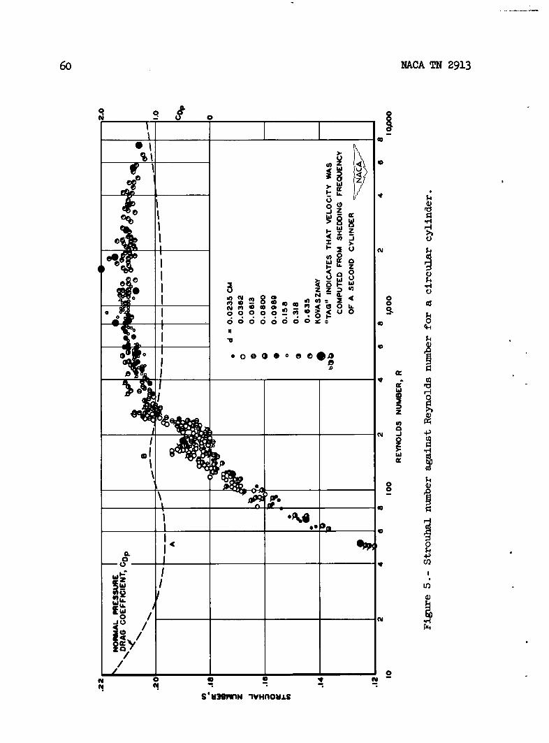
6o MACA TN 2913

C! 0

ww -u

0l0LL

N -(L

m 0

w 00 O O0 O ~ c;0

oI

00ee eo~~V) __

A _ _ _ _ _ _ _ _ _ _ _

to In

cm

w

WU-.

00

J C4

i I /

*7000

S'0 /l _ _ _ _ _ _L

NACA TN 2913 61

cKit 0

0

* 0

* r

x 0

62 NACA TN 2913

co

x9

-n

*i 0

NACA TN 2913 63

8

0

0

00

0 0 4-oooo

0 0

00 00 0

0 0 0;0

000 0

0 0 4

0 0

ooo_ o_ _ __ _ o _ _ o ~

o '° .0

00o 0 0 0 0 0 0 P2

0 00 0 0 w

4)

64 NACA TN 2913

30

25

20

I5

I0

0 040 so s0 100 120 140

Figure 9.- Plot of F against R (50 < R < 140). F =0.212R - 4.5.

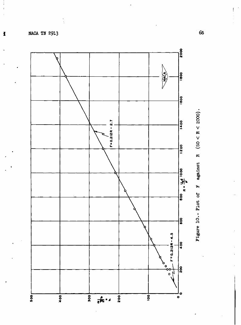
{A4CA TN 2913 65

0

8

00

C4 v

0.0a 0

0 VON0

M

0 to

P4

r-4

4

0H4

_ _ _ _ _ _ _ _ _ _ _ _ _ 8lK 0

Ci30z

IL60k0

80 0 00 ~0000

* e1jpi0a

66 NACA TN 2913

04

(4'

P4

4)

0IIN

- 4

.5- I.

P4

______ _____ _ ___ _ _____ ___ ___ ______ ____In

(4'C I" alf 10

RACA TN 2913 67

00L

11,00

cu E1-4

ca

m tv 1 0 0

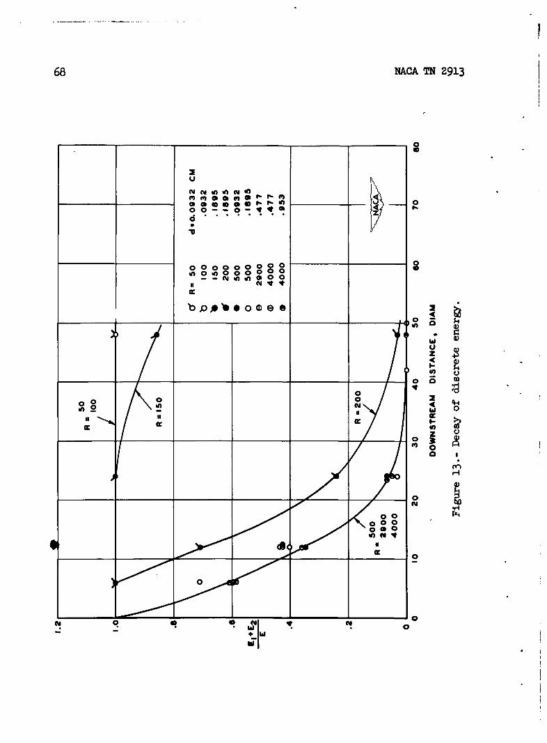
68 NPLCA TN 2913

00~0000 -0

006000

coCoc0W)OC011 C4 V 2mI

z 4)

0~ CY

000

I- V

0 (D030

00 Fu

00

0

00

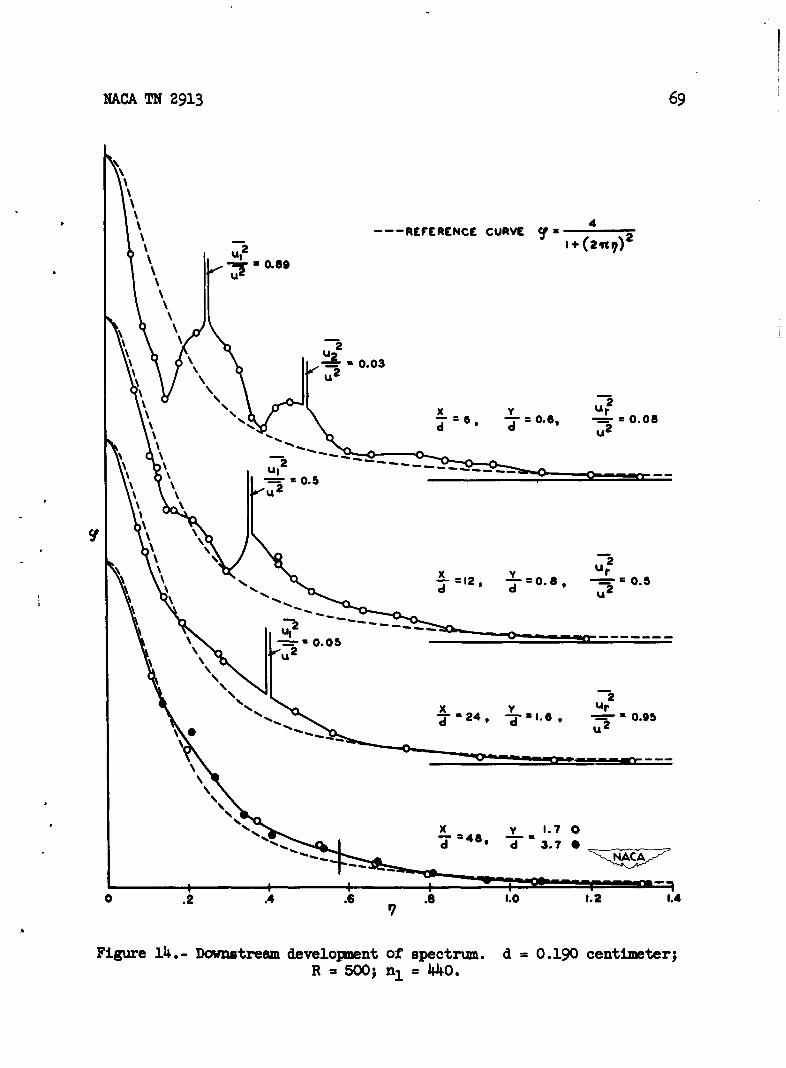
NACA TN 2913 69

~--REFERENCE CURVE C1 4= )

- a 0.89

22

720

U22

2x y

=y 0.6 0.0

02 .. .. .6 ....

R S 0.50;n

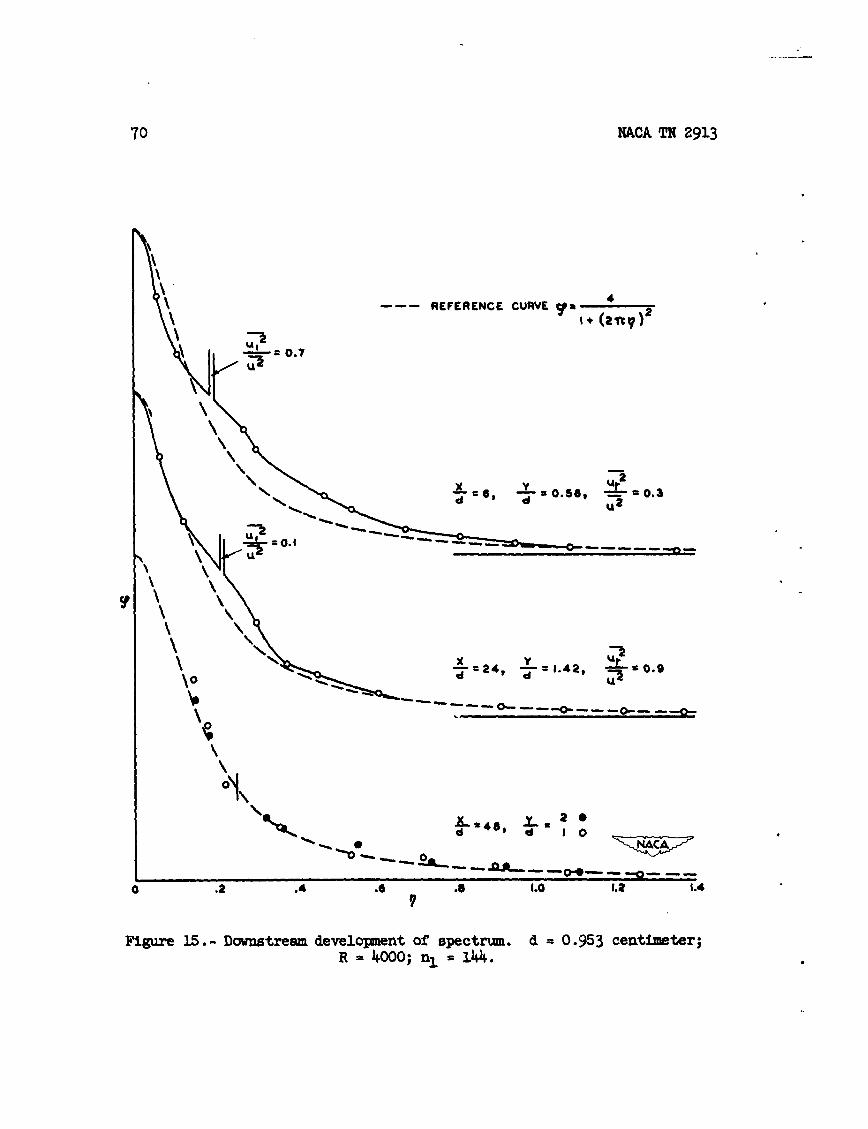
70 NACA TN 2913

REFERENCE CURVE go* +

20. 2

x\ 6, 0-=.38, , - 0.3

01-48, a 1.42,

d 'd 1 0

0 .2 .4 .6 .8 1.0 1.2 1.4

Figure 15.- Downstream development of spectrum. d = 0.953 centimeter;R = 4000; n1 = 14.4.

NACA TN 2913 71

4.0

3.5

2.5-

--- REFERENCE CURVE C

Cy0 .0, 2 09 2r7)

-Y 0.81 4 0.5 3___

'.5-

-pl.0.3

1.0

0.0

.5.

Figure 16. - Spectra, at 12 diameters. d -0.190 centimeter; R = 500;n,= 4+30.

72 NACA TN 2913

4.0

\

I3.5

I0II

3.0 -

I

2.5 1 1I.

2.0 -~- 4---- REFERNCE CURVE Cy - )2

d a 0.953 CM y :0 0

R a 4000 7 2 0

."d a 0.477CM y 0 e

R: 4000 7 3

0 0

d a 0.190 CM y 0 0\e~ ~ z 1 o -17 0

1.0 500 3.7 0

See

'V..o i

0 .2 .4 .6 .6 1.0 1.2 1.4

Figure 17.- Spectra at 48 diameters.

IOH NACA TN 2913 73

CC) 0f

0 .4

C30 0* o4Q r- 00 0

II i,... Lf) .4 -4C'

t o

0

00 0

nrd 0

~rd

74e NACA TN 2913

r 60 oq

en0 4 m e0;o -N mN N ~ _

4 (40

c; *0 0

x- t N qt

0 0 00 0 en-e o oedo o OD

d) C3

I: 0'0a 0

0

0 0i-

00 V

/ILI

0

IL-

NACA TN 2913 75

a, 0

0

0

ILIPd)

orN

* 09

CO

UPH

76 NPLCA TN 2913

12 1.2

G e U0 U9 .

0 0L

4 .4

000

0

-41 1 7.0 10 20 30 X 40 s0 s0

4 .10

.59 (-)/

3 .12

d *.-(FROM STREAMLINES)

2 _ __ _ _ -(FROM U' TRAVERSE) .0

_ _ _ _0 I4

40 5090

Figure 21., Vortex-street geometry. Calculated from data in reference 11.

1H MACA TN 2913 77

z0

0

x -

rd

w

0- *-4

4

,w I.

AA0 0

0) ~ 0

00

0 6*

710

0 -P

hi d d

wx

CC*f.

_______gle -I 3-3-3 00

644

-" i0

H -1

C4 C 4

Q C.

0. -

0. ci W. 140'a0-

ri ;44 'as~ co

Q) o0~ 4)4 * GO! ~ - .C o

0 co 4 E~ w to 'd2 Q)

1, _.' -

0 a2

:5 c 0 -40.

o c o 0 .0 a" 14

- 4 C .'- !3 S e U - 04 -= 4

I4 '--4-,s

. ~ > 0S

0 )> bf

4) -~ E- b c

z 144 1 14)=Q

0

'o

0 44

[-. U)~

-4 or 'm 4 ) S f

1 ~100 x

vi 0: 'm - ai vit 4, U.0 'a

c. i

-6.S..-

S.4

4) C13

I.. t

V- 10

424

0