98
HI/61 Unclas 0021585 https://ntrs.nasa.gov/search.jsp?R=19910016368 2018-07-17T15:27:28+00:00Z

HI/61
Unclas0021585
https://ntrs.nasa.gov/search.jsp?R=19910016368 2018-07-17T15:27:28+00:00Z
NASA Technical Memorandum 4301
The QDP/PLT User's Guide
Allyn F. Tennant
George C. Marshall Space Flight Center
Marshall Space Flight Center, Alabama
National Aeronautics andSpace Administration
Office of Management
Scientific and TechnicalInformation Program
1991


TABLE OF CONTENTS
Page
o Introduction .............................................. 1
1.1 Overview ........................................... I
1.2 Definitions .......................................... 2
1.3 Syntax ............................................. 2
1.4 Questions ........................................... 3
1.5 Acknowledgements .................................... 3
o Basics .................................................. 5
2.1 QDP files ........................................... 52.2 Plot the file ......................................... 5
2.3 Rescaling ........................................... 7
2.4 Making a hardcopy .................................... 8
o Aesthetics ............................................... 9
3.1 Labels ............................................. 9
3.2 Vertical plots ........................................ I0
3.3 Colors, lines,and markers ............................... II
3.4 Log scale ........................................... 12
t Fitting .................................................. 134.1 Errors ............................................. 13
4.2 Fitting ............................................. 144.3 Parameter uncertainties ................................ 16
m Miscellaneous ............................................. 175.1 PLT command files .................................... 17
5.2 Version control ....................................... 18
o Fortran interface
6.1
6.2
6.3
6.4
6.5
6.6
o i i i o o • * * • D D D D D • i o o e o o i D o i t o i o J o i i o i i i i i i i 19
Programming PLT .................................... 19Subroutine RDQDP .................................... 20Subroutine PLT ...................................... 22
The QDP program ..................................... 23The DEMO program ................................... 24A user function ...................................... 26
, COD7.1
7.2
7.3
7.4
7.5
• • ,,, u,,,, i,, J,m IUeUIIDII_J, J, I,, O,,, I • • • J J J J _ , _ m l • 29
Introduction ......................................... 29Interactivemode ..................................... 29
Colon definitions ..................................... 30COD files .......................................... 31
Other stack-oriented languages ........................... 32
Appendix A: COD Command summary .............................. 33
Appendix B: PLT Command summary ............................... 51
Appendix C: QDP Command summary ............................... 75
mL N
..°
Ill
PRECEDING PAGE BLANK NOT FILMED

Appendix D:
Appendix E:
TABLE OF CONTENTS (Concluded)
Page
InstallationguideD.1
D.2
D.3D.4
D.5
D.6
D.7
D.8
D.9
77
77XANADU ......................................77VMS instructions ................................78SUN UNIX instructions ............................
NeXT NextStep instructions ........................ 7878MS DOS instructions ..............................78
Portability .....................................79Relation to PGPLOT ..............................79
Directory structure ..............................80
Porting to other systems ...........................D.9.1 Porting TERMINO software .................... 80
D.9.2 Creating a new SYS.xxx routine ................. 81
D.9.3 Compile and linkthe QDP program ............... 82
Sample plots and QDP files ............................. 83
iv

TECHNICAL MEMORANDUM
TIIE QDP/PLT USER'S GUIDE
Chapter 1
Introduction
1.1 Overview
The Quick and Dandy Plotter (QDP) program reads ASCII files containing various
plotting commands and data. QDP then calls the PLT subroutine which then executes
the commands and plots the data. At this point the "PLT>" prompt appears and the
user can then proceed to enter additional PLT commands which can:
• Display information on about the interactive commands via HElp,
• Override various PLT defaults,
• Override the PLT commands found in the QDP file,
• Add/remove labels,
• Plot data with various combinations of lines, markers, and error bars,
• Change the appearance/style of the of the plot, for example converting all textinto the Roman Font,
• Plot the data as a function of a different x variable,
• Change the number of panels in which the data is plotted,
• Define models and calculate the 'best fit' parameter values,
• Generate a hardcopy.
Thus the interactive PLT commands allow you to both tailor the plot to your
needs/taste and to do some simple analyses of the data. PLT commands can be placed
in the QDP file, in an indirect command and/or in a command array created by the
calling program. For example, if you have a set of commands that you commonly use,
you can place those commands in a file, and then have PLT execute the commands that
it finds in that file. Since exactly the same command syntax is used, it is not necessary
to learn a special programming language to write software that uses PLT. Programmers
can try out PLT commands interactively to find a set that works best with the type of
data being plotted, and then make these commands the default values.
The PLT software is highly portable. It uses the PGPLOT Graphics Subroutine
Library written by T. J. Pearson at the California Ins;itute of Technology. PGPLOT

hasbeenported to manysystemsrangingfrom MS-DOSmachinesto UNICOSCrays.PLT is activelysupportedonVAX VMS, SUNUNIX, andNeXT systems.Thecodeisin standardFortranandsocaneasilybeportedto othersystemsandrunsonMS-DOS,PRIME, andIBM RS/6000systems.
This manualprovidesan overviewof how to usePLT. Not all commandswill bedescribedin the overview.However,AppendixB includesthe contentsof the on-linehelpwhichdoescontaineverycommand.
Therestofthis introductiondefinesafewtermsanddiscussesthesyntaxconventionsused.If youwishto get startedquickly,youshouldskip to thenextchapter.Onceyouhavemasteredthe basics,youshouldcomebackandreadthefollowingsections.
1.2 Definitions
PLT operates on quantities called vectors which can consist of one, two, or three columns
in this rectangular array. If the data contains no errors, then each column is a vector. If
the data contains symmetric errors, then it takes two columns to denote a single vector.
Likewise, if you have two-sided errors (e.g., +5,-2), it will take 3 columns to denote avector. If one number in a vector has an error, then all numbers in that vector must
have the same type of error. The vectors are independent of each other, and so somevectors can have errors and others not.
The PLT default is to make each vector an independent plot group. The PLT SKip
command can be used if you have just two vectors and you wish to create several plot
groups within those vectors.
Viewport denotes the physical area of the plotting surface that you are using.
PLT (via PGPLOT) uses device-independent coordinates to denote the viewport, with
(0.0,0.0) denoting the bottom left corner of the display surface, and (1.0,1.0) the top
right corner.
PLT can be used to fit a model to the data. A model consists of one or more compo-
nents which are added together. Each component must have one or more parameters;
when fitting the data, the parameters are varied to minimize X _. There is no way to
multiply the built-in components together.
A COD file is an ASCII text file that contains a function written in the COD pro-
gramming language. PLT allows you to define a model in which one of the components
is a function contained a COD file. When FIT evaluates that component, the COD func-
tion is called and should return with the function evaluated for the current parameter
set.
1.3 Syntax
PLT does not distinguish between upper and lower case. When PLT matches the
characters you type with possible commands, it only matches characters in the shortest
unique abbreviation which, in this documentation, is denoted by upper case. Thus both
color and colour will match the COlor command. Of course, some caution is required
as cosmopolitan will also match COlor. As new commands are added, a previously
acceptable abbreviation could refer to one of the new commands. To avoid such potential
conflicts, you are encouraged to use three letter abbreviations.
2

In this documentation,anamein all lowercasenameis amnemonicandshouldnotbeentered.Forexample,in Rescale X xrain,xmaxboth "xrain" and "xmax"shouldbereplacedwith numbers.
In PLT, argumentscan be separated by a comma and/or any number of spaces
and tab characters. Thus, the strings i 2 3 , 1,2,3 , 1, 2, 3 , and i , 2 , 3
are all parsed as three arguments. Sometimes it is necessary to leave a place-holder
that indicates an argument should be skipped. This is done by entering two adjacent
commas: The string 1,,3 is parsed as three arguments with the second argument
being null. Null arguments are often used to indicate that the current value should not
be changed. If it is necessary to enter any special character as part of an argument, the
argument should be enclosed in quotation marks. The string 1,"2,3,4",5 would be
parsed as three arguments and the second argument would be the string 2,3,4 .
PLT allows you to embed the simple mathematical operators, + , - , * , and /
into numbers. Thus, the argument 2*3 would be parsed as 6. The numeric expression
is evaluated from left to right; hence, the argument 1+2/4 is parsed 3/4 or 0.75. This
syntax can be useful in QDP files. For example, suppose column 1 is the time in seconds,
and you wish to plot time in hours. This can be done with a global edit that appends
the string/3600, to the numbers in column 1.
The character # is used to denote a number. When you see this character, you
should not type # , but rather replace it with a number. Likewise, the character $
denotes a string. Optional arguments are enclosed in square brackets E...] If an
argument must be one of several discrete choices, the choices will be listed separated by
vertical lines ] .
1.4 Questions
Please address suggestions for improvements, or reports of software bugs, to the author:
Allyn Tennant, ES-65NASA MSFC
ttuntsville, AL 35812USA
Telephone: 205 544-3424FAX: 205 544-7754
SPAN:
Internet:
SSL::TENNANT or 7207::TENNANT
tennant%[email protected]
Please address requests for copies of this manual or the software to:
COSMIC
The University of Georgia
382 East Broad Street
Athens, GA 30602
USA
Telephone: 404 542-3265

1.5 Acknowledgements
These days most non-trivial software packages have evolved over a long period of time
and PLT is no exception.
The first program to bear the name of QDP was written in the late 1970's by Andy
Szymkowiak for use by the X-ray group on a PDP 11/70 at Goddard Space Flight
Center. Although I don't think that a single line of code has survived from that original
version, I am grateful to Andy for that version, and hence for the basic idea of an
interactive graphics program.
The QDP/PLT development flourished during my years at the Institute of Astron-
omy, Cambridge, U.K. I am grateful to Andy Fabian for being able to fund my stay
there, and also for providing the stimulating environment where such working software
could be developed. It is important that PLT was developed not as a software project,
but rather to meet real needs in the analysis of data.
Now that I am at Marshall Space Flight Center, I would like to thank Martin
Weisskopf for his continuing support of these efforts.
I am grateful to Tim Pearson for providing and for continuing to support the PG-
PLOT graphics package. PGPLOT is flexible, easy to use, portable and device inde-
pendent.
Numerous other people have made contributions to PLT, ranging from simple com-
ments, such as "it doesn't work when I do this", to actually providing the code for new
features. Some of these people are mentioned in the on-line help file under the "history"
subtopic. I would like to say thank you to all the people who have offered comments.

Chapter 2
Basics
2.1 QDP files
The quickest and most convenient way to use PLT is with a QDP file. A QDP file is
an ASCII text file that contains a rectangular array of data. Since QDP files are ASCII
they are easy to create and highly portable to different computer systems. All QDP files
must contain a two dimensional array of data. The row-column location of a number in
the file determines the row-column index in the data array passed to PLT. It is possible,
but not necessary, to include QDP and/or PLT commands at the top of the QDP file.
These commands often serve to document the data. All the QDP program does is to
read the file, and to pass the information to the PLT subroutine.
In order to try out the examples in this chapter and the next, you should first create
a "DEM0. QDP" file that contains the following:
1 1 16
2 4 9
3 9 4
4 15 1 ' Yes 15 and N0T 16
(XANADU: [PLOT. QDP]DEM0. QDP contains a pre-typed version of this file.) This example
file contains no QDP or PLT commands. The QDP default is to assume that each
column of numbers is a separate vector.
This example illustrates that QDP files can contain comments. Comments begin
with the comment character ! and continue to the end of the line. The above example
contains the comment "Yes 15 and N0T 16". Comments are completely ignored. This
documentation will often include a comment with the example commands. When trying
out the command, you do not need to type the comment; however, if you do type it,then no harm will be done.
The QDP data lines are free format and the numbers can be separated by spaces,
a comma, or tabs. Every row should contain the same number of columns; however, if
some data are missing, you can enter the word NO instead of an actual number. QDP
translates the NO into the PLT no-data flag; which will be ignored by PLT.
2.2 Plot the file
Once you have created a version of DEM0. QDP, you can run QDP by typing:
$ QDP DEMO

o
XANADU : [I:'LOT.Q D P] D EM O. QD P; 1
2 _ 4-
"f'ENNANT 5--NOV-- leeO 17=12
Figure 2.1: The default appearance of the DEMO. QDP file.
(If QDP fails to run, then you might need to define the QDP symbol as described in
Appendix D, Installation Guide.) It is not necessary to enter the .qDP extension
as the QDP program assumes that as the default. When the program starts, you will
receive the following message:
To produce plot, please enter
PGPLOT file/type :
You should enter the PGPLOT specification for the device on which you wish to plot.
If you do not know the device name, then enter ? and all the device types supported
by your local version of PGPLOT will be listed. If your terminal supports Tektronix
graphics, then enter /TE to make the plot appear on your terminal. You might
also try /RE for Retrographics. Most Tektronix emulators support the Retrographics
extensions that allow the software to toggle between text and graphics modes.
A graph containing two lines will now be drawn as illustrated in Figure 2.1. Since
the file contained three columns of numbers, the default mode assumes there are three
plot groups. The first plot group determines the x coordinate. The next two columns
are plotted as two lines. On a color display the first line will be red and the second
green, which are the default colors for plot groups 2 and 3. The name of the QDP file
appears in the top left of the plot and your userid, current date, and time appear in
the bottom right of the plot. The PLT> prompt will now appear. In the following
sections you will see how to enter various commands to change the default plot. The
most useful command for beginners is the HElp command which can be used to get

instructions on how to use any command.
Another useful command is EXit that will get you out of the PLT subroutine. If
you are in QDP, control will be returned to the operating system; in other programs,
control will be returned to the calling program.
2.3 Rescaling
PLT> R Y 0 20
and
PLT> R Y,,20
PLT> R Y 0
willproduce the same
PLT> R 1 5 1 16 !
PLT chooses a default scale that makes all the data visible. The examples in this section
will illustrate the Rescale command that can be used to change this scale. Using the
plot created in the previous section, enter
PLT> R X 0 5
When you enter this command, the graph is redrawn with 0.0 on the left side and 5.0
on the right side of the viewport. Likewise 1_ Y 0 20 will put 0.0 on the bottom and
20.0 on the top. If you wish to change one number without the other, you can skip the
field with commas or terminate the line before changing the default. For example, both
! Set both lower and upper limit
' Set upper limit to 20, leaving lower unaffected
Set lower limit to O, leaving upper unaffected
effect.Ifyou wish to change both the X and Y limits,then use
Set X-range to I to 5, and Y-range i to 16
If you wish to go back to the default scale, then use R with no arguments:
PLT> h Y ! Will reset V limits to default
PLT> I% ! Will reset both X and Y limits to default
At any time you can find out what the current scale limits are with
PLT> R ?
Current Gap= .025
Window XLAB XMIN XMAX YLAB YMIN YMAX
1 : .9250 , 4. 075 : .6250 , 16.38PLT>
This produces a table of the current scaling parameters. The current gap is the default
size of the gap between the edge of the data and the edge of the plot. For the default
scMe, the difference between the minimum/maximum and the data minimum/data max-
imum is due to the gap. With a gap of zero, the default minimum/maximum value will
exactly match the data minimum/data maximum. The default is to plot all plot groups
into just one window hence only one row appears in the table corresponding to that
window. The columns labeled XLAB and YLAB contain the current x and y labels, which
are currently blank.
If you want to see what the data minimum and maximum values are you should use
PLT> SHow group
Grp Wind Label XData Min XData Max YData Min YData Max
1 -1 : 1.000 , 4.000 : 1.000 , 4.000
2 1 : 1.000 , 4.000 : 1.000 , 15.00
3 1 : 1.000 , 4.000 : 1.000 , 16.00
The three rows correspond to the three plot groups. The column labeled Wind con-
tains the window in which the group is currently being plotted, and a negative number
indicates that the group is not actually plotted. In this example, group 1 is used to
determine the x coordinate and so is not actually plotted. The columns labeled YData
Min and YData Max contain the actual data minimum and maximum of that plot group.
2.4 Making a hardcopy
PLT makes a hardcopy by using the same PGPLOT routines but routed to a different
graphics device. Thus the command does not make a hardcopy of what is currentlyon your screen, but rather, what would be plotted if you reissued the Plot command.
The HArd ? command will display the name of your current default hardcopy device.
It is possible to override this default when you enter the HArd command, thus HArd
/VPS would make a vertical (portrait) mode Postscript file no matter what the default
is. If you would like a default different from what is set up on your system, then you
should define the logical name, or on UNIX, the environment variable, PLT_HARDCOPY
to contain the default you want. Let's assume the default is OK. So, merely enter
PLT> CSize 1.3 ! To increase the character size a bit
PLT> F0nt Roman ! To use the nice looking Roman font
PLT> HArdcopy ! To make a hardcopy file
PGPLOT would have now made a filein your currentdirectory.You should consult
your PGPLOT manual for the ruleson how to printthisfile.On many systems itis
possibleto use the CHARD command thatwillboth createa fileand then spool the file
to the printer.
The default PLT font is the Simple font because it plots the fastest. When you are
making a hardcopy, speed is less important than quality. Therefore, you are encouraged
to use the Roman font, which will give a more professional look to your hardcopy. As
most journals greatly reduce the size of figures before printing, you should increase the
character size. In the above example, CSize 1.3 makes the character size a factor of 1.3
times larger than the default. The default line width is one, which is the thinest possible
line. On some laser printers, this is too thin, and therefore, you should increase the line
width, using the LWidth command. Using LWidth 7 is not unreasonable for publication
quality on some printers. In general the default hardcopy plot will fill the page on
which it is being plotted. If a viewgraph was made of a full page plot, the projected
size would overfill most screens. Therefore, it is useful to decrease the default size of
the plot a bit. This can be done with the Viewport command. The default viewport is
• 1 . 1 which means the box containing the graph extends from 0.10 to 0.90 of the total
physical plotting area. To make a plot half the size, use View .3 .3. View .2 .2 will
result in a good size for most viewgraphs.

Chapter 3
Aesthetics
3.1 Labels
This chapter describes the various options available to change the appearance of the
plot. One of the most common things to do is to add labels, using the LAbel command.
To put the label "Time (sec)" on the x-axis, "Distance" on the y-axis, and "My data"
at the top of the plot,
PLT> LAX Time (see)
PLT> LAY Distance
PLT> LA T My data
PLT> P
You will notice that only certain PLT commands cause the graphics display to be
updated. This allows you to enter severa/ commands quickly without having to wait
for the screen to be redrawn after each command. Whenever you want to see what the
current graph looks like,you should enter the Plol; command or just p.
There are also Outer ]abels (ca/led0X, 0Y, 0T) that can be used. These outer labels
provide a simple way to create labels that need to lieon two lines. For example_ the
commands
PLT> LAX Universal
PLT> LA 0X Time (sec)
PLT> P
would label the z-axis with two lines of text with the word "UnJversaF' being written
above the words "Time (sec)". Now what do you think the following command will do?
PLT> LA 0T Fun! Fun! Fun!
PLT> P
If you try this you will find that only the word "Fun" appears. This is because ! is
the PLT comment character. If you wish to enter a PLT command that contains the
comment character, then you must enclose the entire argument in quotation marks:
PLT> LA 0T "Fun! Fun! Fun!"
PLT> P
To remove any label, enter the command with no text; thus,
PLT> LA 0T
PLT> P
9
will removethe text "Fun! Fun! Fun!" from the graph. The nameof the QDP fileappearsin the File position; thusthe command LA F will remove this name. The
time-stamp that appears at the bottom of the plot can be removed with the Time 0Ff
command and, of course, Time 0N will turn it back on. In general, you should leave
the file name and time-stamp in place, as this information is very useful on a hardcopy.
Sometimes, when working with a slow plotting device, you will want to speed things up
by not plotting any labels. This can be done the LAbel 0Ff command. Of course,
you should issue the LAbel ON command before making a hardcopy.
Text is drawn with PGPLOT; so the standard PGPLOT escape sequences are used.
Hence, the commands
PLT> LA T \gx\u2
PLT> P
will label the top of the graph with X 2. The default font is the PGPLOT Normal font,
which draws rather quickly. For journal quality text, you should override the default
font with the FOnt Roman command. This will cause all text, including the numeric
labels on the axes, to be written in the nicer looking, but slower plotting, Roman font.
Use FOnt ? to get alist of possible fonts.
It is also possible to place a numbered label anywhere in the plot. To see this, try
PLT> LA 1 Pos 2 4 Line -45 "Point at (2,4)"
PLT> P
The above command plots LAbel 1 at Position (2,4) with a Line extending at an angle
of-45 ° to the x-axis and with the text message "Point at (2,4)". Each attribute can be
set individually. IIence, if you decide you don't like the line extending downwards, you
could change the angle with
PLT> LA i Line 135
PLT> P
This leaves the pointing position and text unaffected, but resets the angle of the line
(and also the justification of the string).
3.2 Vertical plots
When you first plotted the DEM0.QDP file, two plot groups were plotted on the same
panel. It is possible to plot each plot group on a separate panel in a vertical stack. To
see this, try
$ QDP DEM0
(enter device type)
PLT> Plot Vertical
PLT> Plot
The Plot Vertical command resetsthe internal parameters so that each visibleplot
group will be plotted in a separate panel in a vertical stack. Nothing is replotted until
the Plot command alone is issued. This allows you to reset other parameters, without
having to wait for a new graph to be drawn.
The y-scale can be adjusted in each panel separately. Hence,
PLT> R Y2 0 10
PLT> R Y3 0 50
PLT> P
10
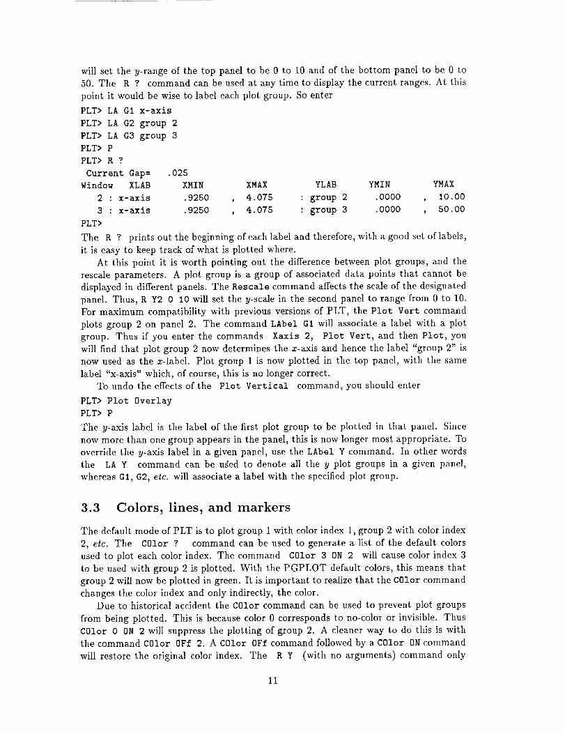
will set the y-range of the top panel to be 0 to 10 and of the bottom panel to be 0 to
50. The R ? command can be used at any time to display the current ranges. At this
point it would be wise to label each plot group. So enter
PLT> LA G1 x-axis
PLT> LA G2 group 2
PLT> LA G3 group 3
PLT> P
PLT> R ?
Current Gap= .025
Window XLAB XMIN XMAX YLAB YMIN YMAX
2 : x-axis .9250 , 4.075 : group 2 .0000 , i0.00
3 : x-axis .9250 , 4.075 : group 3 .0000 , 50.00
PLT>
The R ? prints out the beginning of each label and therefore, with a good set of labels,
it is easy to keep track of what is plotted where.
At this point it is worth pointing out the difference between plot groups, and the
rescale parameters. A plot group is a group of associated data points that cannot be
displayed in different panels. The Rescale command affects the scale of the designated
panel. Thus, R Y2 0 10 will set the y-scale in the second panel to range from 0 to 10.
For maximum compatibility with previous versions of PLT, the Plot Vert command
plots group 2 on panel 2. The command LAbel G1 will associate a label with a plot
group. Thus ifyou enter the commands Xaxis 2, Plot Yert, and then Plot, you
will find that plot group 2 now determines the x-axis and hence the label "group 2" is
now used as the x-label. Plot group I isnow plotted in the top panel, with the same
label "x-axis" which, of course, this is no longer correct.
To undo the effectsof the Plot Vertical command, you should enter
PLT> Plot Overlay
PLT> P
The y-axis label is the label of the firstplot group to be plotted in that panel. Since
now more than one group appears in the panel, this isnow longer most appropriate. To
override the y-axis label in a given panel, use the LAbel Y command. In other words
the LA Y command can be uged to denote all the y plot groups in a given panel,
whereas GI, G2, etc. will associate a label with the specifiedplot group.
3.3 Colors, lines, and markers
The default mode of PLT is to plot group 1 with color index 1, group 2 with color index
2, etc. The COlor ? command can be used to generate a list of the default colors
used to plot each color index. The command COlor 3 ON 2 will cause color index 3
to be used with group 2 is plotted. With the PGPLOT default colors, this means that
group 2 will now be plotted in green. It is important to realize that the COlor command
changes the color index and only indirectly, the color.
Due to historical accident the COlor command can be used to prevent plot groups
from being plotted. This is because color 0 corresponds to no-color or invisible. Thus
COlor 0 ON 2 will suppress the plotting of group 2. A cleaner way to do this is with
the command COlor OFf 2. A COlor OFf command followed by a COlor 0N command
will restore the original color index. The R Y (with no arguments) command only
11

usesplot groupsthat arevisible to determinethe defaultscale.For example,assumeyouareworkingwith 6 plot groupsand thevaluesof groups1 to 5 all lie in the rangeof 0.0to 1.0,whereasthe valuesin group6 all lie near100,000.For this example,thecommands
PLT> COlor 0FF 6
PLT> R Y
would redraw the graph, and the default y-range will lie between 0.0 and 1.0.
In the above examples, PLT drew a line between the points being plotted. If you
wish to display the plot with markers, then you should turn on the plotting of markers
with
PLT> MArk ON
PLT> P
For this example, the line connecting the various points disappears and only markers
will be drawn. PLT draws a linewhen (a) all attributes (Line, MArker, and Errors)
are 0FF or (b) the line attribute is 0N. Thus if you want both the connecting line and
markers to appear, then you need to turn on the Line attribute with
PLT> Line 0N
PLT> P
The command MArker Size 2 can be used to make the markers twice as big.
The default marker style for allplot groups istype 2 as this marker plots very quickly.
To change the style of the marker, try MArker 9 0N 2 to use marker style 9 when
plotting group 2. The command MArker ? will display a table of marker styles.
3.4 Log scale
It is also possible to plot the data on a log scale. To do this, type
PLT> L0g YPLT> P
Use LOg X to use a log scale on the x-axis. The LOg OFf command will turn off the
log scale on both the x- and y- axes. Note: Using LOg does not cause the data to be
altered, only the appearance of the l_lot changes. If the lower limit of the scale being
logged is negative or zero, then PLT will rescan the data searching for the smallest
positive value, and make that the lower limit.
You should also be aware of the fact that the size of the gap, created by the GAp
command is affected by log scale. Thus for a non-zero gap, the sequence R X followed
by LOg X produces a different range than LOg X followed by R X. In the first case, the
data minimum and maximum values are found, and then gap added in linear space.
Applying the LOg command does not change this scale. In the second case, the scale is
first logged, then the data minimum and maximum values are found. At this point the
correct gap for a log plot is added.
12

Chapter 4
Fitting
4.1 Errors
This section describes a QDP file that contains errors and how to control the plotting
of those errors. The next two sections describe how to define a model, find the best
fitting parameter vaiues, and then estimate the uncertainties on the parameter values.
Although the examples will be based on the QDP file containing errors, it is possible
(and sometimes better) to fit data without errors.
You should now create a DEM01. ODP file that contains the following:
READ Serr I 2
LAbel X Time
LAbel Y Distance
1.0 .95 1.24 .3
i.5 .25 1.86 .3
2.0 .25 3.76 .3
4.0 i.75 16.43 .3
7.0 1.25 49.06 .3
The first line in this file is not a PLT command but rather a QDP command. The QDP
READ command is used by QDP to tell PLT which vectors contain errors. In this case
the READ command tells QDP that vectors 1 and 2 will have symmetric errors; hence,
columns 1 and 2 contain data and errors for vector 1, and columns 3 and 4 contain data
and errors for vector 2. Following the QDP command are two PLT commands that will
be passed to the PLT program and executed before the graph is drawn. Including PLT
commands in the QDP file provides a way to override built-in defaults and/or to add
labels to the graph. Data lines occur after all the command lines. To read and plot this
file, use
$ QDP DEMOI
(enter device type)
PLT>
The graph which looks like Figure 4.1 should now appear. When you plot data contain-
ing errors, the error attribute is ON, and the errors plotted. As described in Section 3.3,
the line will no longer appear connecting the data. If you want to see that line, then
should use Line ON to explicitly switch on the line. To suppress plotting of the errors
use_
PLT> Error OFf
13

otr_
o
o
o
XANADU:[PLOT. QDP]DEMO 1 .QDI:_; 1
i i iI
__l_._ ---h-----
2 4- 6
Time
Figure 4.1: The default appearance of the DEM01.qDP file.
PLT> P
This disables plotting of the error bars. Once again the line connecting the points
appears. You should now enter
PLT> Line StepPLT> P
to produce a stepped-line plot. Using Error ON at this time will cause both the
stepped line and the errors to be plotted. This is because the Line Step command
sets an internal flag that a line should be plotted and the Error 0N command sets
another flag to plot errors. The command Line 0Ff will turn off the plotting of the
(stepped) line. The plotting of a line, errors and markers can all be turned on or off for
each vector independently. See the Line, Error and MArker commands, in Appendix B,
PLT Command Summary, for more information.
4.2 Fitting
This section requires the DEM01. QDP file described in the previous section. Before you
can fit data, you must first define a model. First, read in the data and define a constantmodel with
$ QDP DEMOI
(enter device type)
PLT> MOdel CONS
14

At thispoint, youwill bepromptedfor the defaultinitial valuefor the constant.Enter_Return_ to use the default, and at the PLT> prompt, type Fit} When Fit runs, itfirst tells you which plot group is being fitted and the range over which data are being
fitted. It is important to realize that if you have used R X to rescale the x-axis so
that some points are outside the range plotted, then these points would not be included
in the fit. You cannot exclude points using the R Y command. (This is intended to
prevent cheating.) You will next see the message "Fitting 5 points in a band of 5". This
informs you that there are 5 points in the current x-range. In order to execute faster,the FIT routine resets the minimum and maximum of the array, to achieve the smallest
range possible that includes all points in the x-range, and so the "band of 5" output
informs you how big this minimum range is. Next the FIT routine prints the current
parameter values (1.00000 in this case). The program then prints the current value of
the weighted variance W-VAR. If you have errors on your data, the weighted variance is
_2; for no errors, W-VAR is just the variance. The number in () is log A and is for the
expert's use.
The CURFIT routine will terminate when the change in X 2 or, for an unweighted
fit the relative change in the variance, is less than 0.05. If this condition has not been
met after 10 iterations, you will be prompted "Continue fitting? (n)" Answer Y tocontinue or N to terminate. If you are are fitting in background or batch mode, then
you should always leave a blank line after the Fit command. Thus if Fit does not
terminate, the "Continue fitting? (n)" question will read the blank line with thedefault answer of "no" and terminate. If the fit does terminate, PLT will see the blank
line, and ignore it. When CURFIT terminates, the current parameter values are again
printed and this model is drawn on the current plot.
For the above, the total variance is 18323 and hence a CONS does not look like a
very good model. Let's try a more complicated model with
PLT> MOdel CO LI QU
to include constant, linear and quadratic components. Again you can default on all the
initial values. When you type Fit, you should find that W-VAR has decreased to 4.23.
This is clearly a better fit.
To generate a list of all possible built-in components, use the MOdel ? command.
To obtain a description of what a component does, use the HElp MOdel command
followed by the component name. If you can not construct your model from the built-in
components, then you can create additional components. A COD file can be used to
define a sophisticated component. COD files are ASCII text files that contain functions
written in a Forth-like computer language. Chapter 7 and Appendix A describe COD
in some detail. If your component is too complicated for COD, or you don't like using
COD, then you can create a Fortran function that can be used as a new component.
The next chapter will describe how to create this function UFNY, and the supporting
routines to replace the built-in DEN0 component.
It is possible to save the current model to a disk file using the WModel command.
For example,
PLT> WModel DEMOI
1The FIT subroutine minimizes X2 using a modified version of Bevington's CURFIT subroutine.Bevington's book Data Reduction and Error Analysis for the Physical Sciences, published by McGraw-Hill in 1969, is an excellent introduction to statistics. Anyone interested in a detailed understanding ofhow CURFIT works should consult this book.
15

will create a DEM01.MOD file. To read this model back into PLT use the command
MOdel ©DEM01. Model files can be printed out to make a hardcopy of the current
parameter values. If you do not enter a file name with the Wgodel command, then the
model is written to your current terminal screen.
4.3 Parameter uncertainties
The Uncertainty command can be used to estimate the uncertainties in the parameter
values. 2 To try this, you should first fit the data in the DEMOi. QDP file to a CO LI QU
model, as described in the previous section. Now enter the command
PLT> Uncertain I
The program will now change the value of parameter 1 by a small amount and recom-
pute X 2. At each step, the delta parameter value and the AX 2 are printed out. For
complicated models it may take many steps before the desired value of AX 2 is found.
The program considers both positive and negative delta parameter values. The de-
fault value of AX 2 is 2.7 which corresponds to the 90% confidence range for a single
parameter.
With the DEM0i.QDP file you will find that both parameter 1 and 2 are consistent
with zero. To see whether they can be eliminated, try the following:
PLT> Newpar 1,0,-i
PLT> Newpar 2,0,-1PLT> Fit
The first command resets both the VAL and SIG terms of parameter 1 to be 0.0 and -1.0,
respectively. A SIG of -1.0 means that the parameter is frozen and hence not allowed
to change. Note: The command Newpar 1, ,-1 would have frozen parameter 1 at its
current value. The second line freezes the value of parameter 2 to be zero. The results
of the Fit reveal that X 2 has increased by 0.55 and the F-statistic or a likelihood ratio
tells us that these two components were not required by the model.
The Uncertainty command is fairly robust but on occasion can have difficulties.
Sometimes, Uncertainty will find a new minimum value of X 2. This causes the search
to be stopped and the parameter values to be reset. At this point, you should re-issue
the Fit command to locate precisely the new minimum. Sometimes, Uncertainty will
be unable to locate the requested value of AX 2 after l0 tries. At this point the message
UNCERT--Give up. is printed. It will be up to you to decide whether the error has
been correctly calculated. Finally, the Uncertainty command uses the SIG value to
estimate the location of the error. If this number is greatly in error, then Uncertainty
will be starting its search in the wrong place. If this occurs, then it is sometimes possible
to adjust SIG to be a more accurate estimate, before issuing the Uncertainty command.
It is also possible that the SIG is inaccurate because the true minimum has not been
found and further fitting is needed.
2Uncertainties in parameter values are estimated using the method described in "Parameter Estima-tion in X-ray Astronomy", by M. Lampton, B. Margon, and S. Bowyer, in The Astrophysical Journal
(1976) Vol. 208, p. 177.
16
Chapter 5
Miscellaneous
5.1 PLT command files
PLY commands can also be entered via a command file. For example, if you often enter
the sequence of commands FOnt Roman followed by CSize 1.3, then you could createa file called NICE.PC0 that contains the lines
FOnt Roman
CSize I.3
To execute these commands inside PLT, all you need to type is
PLT> @NICE
A default file extension .PC0 is assumed. Thus command files provide a way to enter
several and/or complicated commands easily.
Note that the reference to a command file is a legal PLT command that can appear
in a QDP file. Since this is a PLT command, QDP itself will not open and read the
command file. Hence, QDP commands and data lines cannot be entered via a command
file. Command files serve two important uses in QDP files. First, they provide a way
to enter the same set of commands to several files. Second, for long data files, editing
the QDP file can be tedious. Hence, you can edit it once to enter a reference to the
command file. Thereafter, whenever you want to change the PLT command list, you
need only to edit the command file.
PLT searches up to three different directories for the specified indirect command.
The current directory is always searched first. If the file is not found in the current
directory then PLT tries to translate the logical name (under VMS) or environment
variable (under UNIX or DOS) called MY-XCOMS. If MY_XCOMS has been defined,
then PLT searches the specified directory. If the file still has not been found then
PLT searches the XANADU:[LIB.XCOMS] directory. This three level search allows you to
create system-wide files, user-wide files, and directory specific files. For example, many
locations create a file HARD.PCO in the XANADU: [LIB.XCOMS] directory that (1) creates a
hardcopy file and (2) spools the file to the printer (done using the $ command to spawn
a job to spool the plot to the printer). This then allows all users on that system to use
PLT> @HARD
to immediately print a hardcopy. If you do not like something about the existing @HARD
command then you can easily create a new private version of this command. First copy
the file to one of your own directories, modify the file, and define MY_XCOMS to contain
17

the nameof the directorycontainingthe newversion. Oncethis hasbeendone,PLTwill find and run yourversionof the commandinsteadof thesysteminstalledversion.
It is possibleto useparameterswith indirectcommandfiles. Theparametervaluesareenteredon the sameline that openedthe indirectcommandfile. Thus,PLT> _test one two three
would cause PLT to open and read the TEST.PC0 file with three parameters "one",
"two", and "three". If n is a number then the sequence %n% will be replaced with
the nth parameter. For the above example, %1% will be replaced with 'one', %2% with
'two', etc. The following illustrates a possible indirect file that could use up to three
parameters:
LABel X %1%
LABel Y %2%
LABel T 7.37.
If you fail to enter all three parameters, then %n%will be replaced with a null string for
the unentered parameters.
It is possible for one indirect file to call another indirect file and pass in parameters.
Thus,
©deeper first %2% %3%
is a valid line in an indirect command file. In this example, the first parameter is
"first", whereas the next two parameters will be set equal to parameters 2 and 3 of
the current script. Also quotes can be used to denotes a single parameter with embedded
spaces, or other 'magic' characters. Thus the line,
©file "This is all one" two three
contains three parameters, and the first parameter is the string 'This is all one'.
5.2 Version control
New features are constantly being added to PLT, and so it is important to keep track of
these changes. There are three places where changes are noted. First, the PLT VErsion
command can be used to identify the date of the most recent change to the version of
PLT linked into the program you are using. If certain commands do not appear to work
then you should check this number. Often you will find that the program has not been
linked for a while and as a result the command that you are trying to use was addedafter the last link.
The second place in which version numbers are recorded is the on-line help file. The
HElp VErsion command will list all recently-added new features and when they were
made. A serious attempt is made to ensure that on-line help is updated as the software
is modified. For best results on your system, you should also update the on-line help
every time you update PLT itself. However, there is no requirement for these two version
numbers to match. Thus, when you install a new version of PLT it is not necessary to
immediately relink all software that uses it.
Finally the printed manual is updated about once a year. Therefore, it can be
slightly out of date.
18
Chapter 6
Fortran interface
6.1 Programming PLT
After using the QDP/PLT software for a while, some people would like to see more
sophisticated features such as the ability to read binary files, or to add different vectors
together. Although the author is always willing to take suggestions (and even to ira-
plement some of these suggestions), the PLT design goal is to implement new features
in as general manner as possible. Thus if you need to read a particular file format, or
to manipulate data in a particular manner, you should implement your own front end
to the PLT subroutine. This is simple to do since the QDP program cleanly separates
reading of the file from actually calling the PLT routine.
This chapter describes how to call the RDQDP and PLT subroutines. Also listed
is the complete source code for tl_e QDP program. Although QDP can be used as an
example of how to call PLT, it is perhaps too simple. Therefore the DEMO Fortran
program more clearly shows how to do this. Finally there are instructions on how tocreate your own user-defined function that, when linked with the QDP/PLT software,can be used with the Model and Fit commands.
Although PLT uses several other internal routines, you are discouraged from directly
using these routines in your code. This is because PLT continues to evolve, and there is
no way that the author can add the functionality required without the ability to modify
the internal interfaces. There are no plans to modify the calling sequence for all the
routines described in this chapter.
19

6.2 Subroutine RDQDP
The calling sequencer or the RDQDP subroutine is:
SUBROUTINE RDQDP(ICHAT, LUNIN, CNAM, Y, MXPTS, IERY, MXVEC,
: NROW, NPTS, NVEC, CMD, MXCMD, NCMD, IER)
INTEGER MXPTS, MXVEC, MXCMD
CHARACTER CNAM*(*), CMD(MXCMD)*(*)
REAL Y(MXPTS)
INTEGER IERY(MXVEC)
INTEGER ICHAT, LUNIN, NROW, NPTS, NVEC, NCMD, IER
------
C Opens and reads a QDP file.
C------
C ICHAT
C LUNIN
C CNAM
CY
C MXPTS
C IERY
C MXVEC
C NROW
C NPTS, NVEC
C CMD
C NCMD
C IER
I >i0 means print comment lines, >0 print row/col info.
I <>0 means file already open on LUN.
I/0 File name.
0 Tne data array
I The actual size of the Y array.
0 The PLT error flag array
I The actual size of the IERY array
0 Maximum number of rows that the file could contain.
0 Needed by PLT
0 Command array (MXCMD input dimension).
0 Number of commands read
0 =-i if user entered EOF, =0 file read, =I no file read.
There are several ways to specify a file to be read by RDQDP. RDQDP will go
through the following steps to determine what file to read. Once a file has been deter-
mined the remaining steps will be skipped. Specifically RDQDP will do the following:
• If the variable LUNIN is non-zero then RDQDP will assume that the input file has
already been opened and is attached to the specified unit number.
• If the variable CNAM is non-blank, then RDQDP opens a file with the specified
name.
At this point it is necessary to obtain a file name from an external source and the
parser is called to handle this. If this is the first time the parser has been called
in the current program, an attempt will be made to read the command line. If a
QDP file name is found on the command line, then that file is opened.
If no file name could be found, or the file could not be opened, then RDQDP will
prompt the user for an input file name. If the user enters an end-of-file ('Z under
VMS, or/* under all systems), then RDQDP will exit with IER=-I. If the user
enters a blank line for the file name, RDQDP will exit IER>0. Of course, if the
user enters a valid file name, then that file is opened, and IER will return a value
of 0.
Once a file has been opened, and if MXCMD>I, RDQDP will add a LAbel F command
to the CMD array that contains the name of the file actually opened. Of course, if the file
2O

contains a LAbel F command, then that command will overwrite the label that RDQDPcreates.
ICHAT is the 'chatter' flag. If ICHAT>10 then RDQDP will display lines that have
! in the first column, on your terminal screen. Displaying these lines, provides a useful
way to confirm that RDQDP has opened the correct file. Such comment lines are
completely ignored, and the comments will be removed from any other line containing
a comment. RDQDP examines the beginning of each line and if the line contains a
QDP command, RDQDP proceeds to interpret the command and set the appropriate
variables to be passed to PLT. If the line starts with a PLT command and NCMD<MXCMD,
then RDQDP will increment NCMDand add the line to the CMDarray. For lines containing
data, RDQDP interprets the line into real numbers and stores these numbers in the Y
array.The RDQDP routine does not open and read any indirect command files, but just
stores the command in the CMDarray. Therefore you cannot use an indirect command
file to contain the data array. Since the calling program determines the size of the CMD
array it is sometimes useful to store all PLT commands in an indirect command file and
to add one line to the QDP file to read the indirect file. When PLT reads an indirect
file it will accept command lines up to 250 characters long, and there is no limit to thenumber of lines that can be read.
When RDQDP reads the first data line, it determines the number of columns in
that line. Based on the number of columns, and the size of MXPTS passed in, RDQDP
calculates the maximum number of rows that would fit into the Y array. If the ICHAT> 0,
RDQDP will then display on the terminal the number of columns, the numbers of vectors
(calculated from the data from in any READ lines), and the maximum number of rows.
21

6.3 Subroutine PLT
The calling sequence _rthe PLT subroutineis:
SUBROUTINE PLT(Y, IERY, MXROW, NPTS, NVEC, CMD, NCMD, IER)
REAL Y(*)
INTEGER IERY(*), MXRDW, NPTS, NVEC, NCMD, IER
CHARACTER CMD(*)*(*)
C------
C General plot subroutine.
C---
c Y(,) IC
C
C
C
C
C IERY (*) I
C
C
C
C MXROW I
C NPTS I
C NVEC I
C CMD(*) I
C NCMD I
C IER O
The data array. The array should be dimensioned
Y(MXROW,MXCOL) where MXROW and MXCOL are the actual
sizes of the arrays in the calling program.
MXCOL=NVEC+NSERR+2*NTERR where NSERR is the number
of vectors that have symmetric errors and NTERR
is the number of vectors that have two-sided errors.
=-i plot errors as SQRT(Y)
= 0 no errors.
=+i explicit symmetric errors.
=+2 for two-sided errors
The actual first dimension of the Y array.
The number of points to plot (NPTS<=MXROW).
The number of vectors to be plotted.
Array of commands.
Number of commands.
Error flag, =-I if user entered EOF, =0 otherwise.
It is important to remember that the variable NVEC does not refer to the number of
columns of data but rather the number of vectors. Each vector must have one en-
try in the IERY array that describes the type of error on that vector. Depending
on the type of error, each vector can be composed of one, two, or three columns of
data. To calculate the number of columns needed by the vectors, let NSERR be the
number of vectors with symmetric errors (IERY(I)=I) and NTERR the number with
two sided errors (IERY(I)=2). The total number of columns MXCOL will be given by
MXCOL=NVEC+NSERR+2*NTERR.
The variable MXROW contains the physical first dimension of the Y array. Thus the
calling program should dimension Y to be (MXROW,MXCOL) or the Fortran equivalent
(MXROW*MXCOL). The variable NPTS contains the number of rows that contain valid data.
All rows from NPTS+I to MXROW will be ignored. When PLT starts it will execute NCMD
lines from the CMD array. Any valid PLT command can be entered into this array. For
example, one line could contain a reference to an indirect command file, and this would
cause PLT to execute all commands found in this file. If the command list contains the
EXit command, then PLT will exit when this command executes and any commands
following the EXit will be ignored. Since PLT does not actually plot any data until all
the commands are executed, it is a good idea to precede an EXit with a Plot command,
since that will force a plot to be produced.
If PLT exits normally, i.e., with the the EXit command, then IER is set to zero. If
the user enters an end-of-file then PLT exits with IER<0.
22
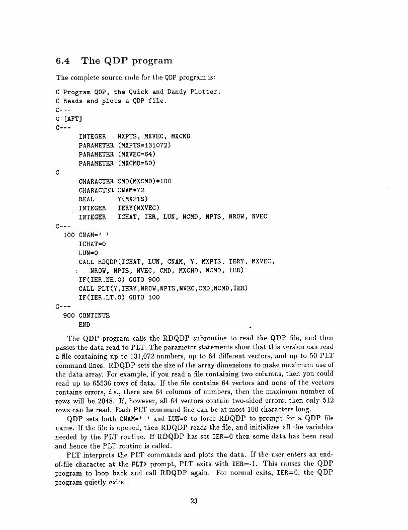
6.4 The QDP program
The complete source code for the QDP program is:
C Program QDP, the Quick and Dandy Plotter.
C Reads and plots a QDP file.
___
C [AFT]
C-----
INTEGER MXPTS, MXVEC, MXCMD
PARAMETER (MXPTS=I31072)
PARAMETER (MXVEC=64)
PARAMETER (MXCMD=50)
CHARACTER
CHARACTER
REAL
INTEGER
INTEGER
CMD(MXCMD)*IO0
CNAM*72
Y(MXPTS)
IERY(MXVEC)
ICHAT, IER, LUN, NCMD, NPTS, NROW, NVEC
CNAM=' '
ICHAT=O
LUN=O
CALL RDQDP(ICHAT, LUN, CNAM, Y, MXPTS, IERY, MXVEC,
: NRDW, NPTS, NVEC, CMD, MXCMD, NCMD, IER)
IF(IER.NE.O) GOTO 900
CALL PLT(Y,IERY,NROW,NPTS,NVEC,CMD,NCMD,IER)
IF(IER.LT.O) GOTO i00
CONTINUE
END
The QDP program calls the RDQDP subroutine to read the QDP file, and then
passes the data read to PLT. The parameter statements show that this version can read
a file containing up to 131,072 numbers, up to 64 different vectors, and up to 50 PLT
command lines. RDQDP sets the size of the array dimensions to make maximum use of
the data array. For example, if you read a file containing two columns, then you could
read up to 65536 rows of data. If the file contains 64 vectors and none of the vectors
contains errors, i.e., there are 64 columns of numbers, then the maximum number of
rows will be 2048. If, however, all 64 vectors contain two-sided errors, then only 512
rows can be read. Each PLT command line can be at most 100 characters long.
QDP sets both CNAM=' ' and LUN=0 to force RDQDP to prompt for a QDP file
name. If the file is opened, then RDQDP reads the file, and initializes all the variables
needed by the PLT routine. If RDQDP has set IER=0 then some data has been read
and hence the PLT routine is called.
PLT interprets the PLT commands and plots the data. If the user enters an end-
of-file character at the PLT> prompt, PLT exits with IER=-I. This causes the QDP
program to loop back and call RDQDP again. For normal exits, IER=0, the QDP
program quietly exits.
23
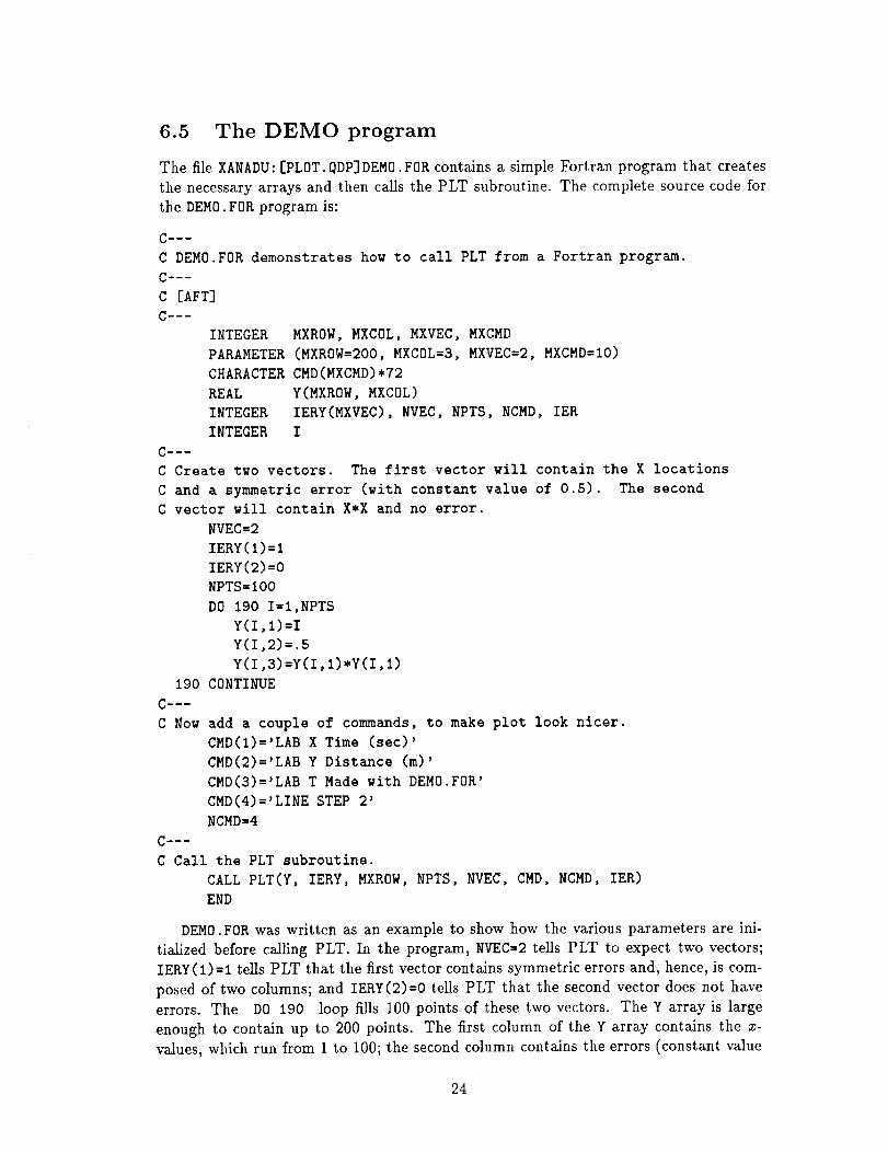
6.5 The DEMO program
The file XANADU: [PLOT. {:)DP] DEM0. FOR contains a simple Fortran program that creates
the necessary arrays and then calls the PLT subroutine. The complete source code for
the DEMO. FDR program is:
C---
C DEM0.FOR demonstrates how to call PLT from a Fortran program.
C---
C [AFT]
------
INTEGER MXROW, MXCOL, MXVEC, MXCMD
PARAMETER (MXROW=200, MXCOL=3, MXVEC=2, MXCMD=IO)
CHARACTER CMD(MXCMD)*72
REAL Y(MXROW, MXCOL)
INTEGER IERY(MXVEC), NVEC, NPTS, NCMD, IER
INTEGER I
C--'--
C Create two vectors. The first vector will contain the X locations
C and a symmetric error (with constant value of 0.5). The second
C vector will contain X*X and no error.
NVEC=2
IERY(1)=I
IERY(2)=O
NPTS=IO0
DO 190 I=I,NPTS
Y(I,I)=I
Y(Z,2)=.sY(I,3)=Y(I,I)*Y(I,I)
CONTINUE190
------
C Now add a couple of commands, to make plot look nicer.
CMD(1)='LAB X Time (sea)'
CMD(2)='LAB Y Distance (m)'
CMD(3)='LAB T Made with DEMO.FOR'
CMD(4)='LINE STEP 2'
NCMD=4
------
C Call the PLT subroutine.
CALL PLT(Y, IERY, MXROW, NPTS, NVEC, CMD, NCMD, IER)
END
DEM0.FOR was written as an example to show how the various parameters are ini-
tialized before calling PLT. In the program, NVEC=2 teUs PLT to expect two vectors;
IERY(1)=I tells PLT that the first vector contMns symmetric errors and, hence, is com-
posed of two cdumns; and IERY(2)=0 tells PLT that the second vector does not have
errors. The DO 190 loop fills 100 points of these two vectors. The Y array is large
enough to contmn up to 200 points. The first column of the Y array contains the x-
values, which run _om 1 to 100; the second column contains the errors (constant value
24

0.5); and the third column contains x 2. After the Y array is initialized, the CMDarray isinitialized with four PLT commands. The first three commands define labels, and the
last command creates a stepped-line plot.The file XANADU:[PLOT. QDP] DEM0. COMwill compile and link the DEM0. FOR program
on a VMS system. This file can be used as an example for linking other routines that call
PLT. It is necessary to link with both the XANLIB library and the PGPLOT graphics
library.
25

6.6 A user function
The calling sequences for the four subroutines required to create a user component are:
SUBROUTINE UINF0(IPAR, CNAME, NPAR)
INTEGER IPAR, NPAR
CHARACTER CNAME*(*)
C---
C IPAR I
C CNAME 0
C
C NPAR O
C-----
C*********
SUBROUTINE ULIMIT(PVAL, PLIM, NT, NPAR)
REAL
INTEGER
------
C PVAL(*) I/0
C PLIM(I,*) I
C NT I
C NPAR I
C-----
C*********
The parameter number.
The name of the parameter IPAR. Note if IPAR=O, then
-return the name of the model.
The number of parameters in your user model.
PVAL(*), PLIM(3,*)
NT, NPAR
The current parameter values
If <0 then the corresponding parameter is frozen
Pointer to first parameter value in array PVAL(*)
Number of parameters
REAL FUNCTION UFNY(X, PVAL, NT, NPAR)
REAL X, PVAL(*)
INTEGER NT, NPAR
I
I
I
I
The current X value
The current parameter values
Pointer to first parameter value in array PVAL(*)
Number of parameters
C---
CX
C PVAL
C NT
C NPAR
C---
C_********
SUBROUTINE UDERIV(X, PVAL, PLIM, DERIV, NT, NPAR)
REAL X, PVAL(*), PLIM(3,*), DERIV(*)
INTEGER NT, NPAR
I The current X value
I The current parameter values
I The constraints array
0 The calculated derivative
I Pointer to first parameter value in array PVAL(*)
I Number of parameters
C---
CX
C PVAL
C PLIM
C DERIV
C NT
C NPAR
C------
26
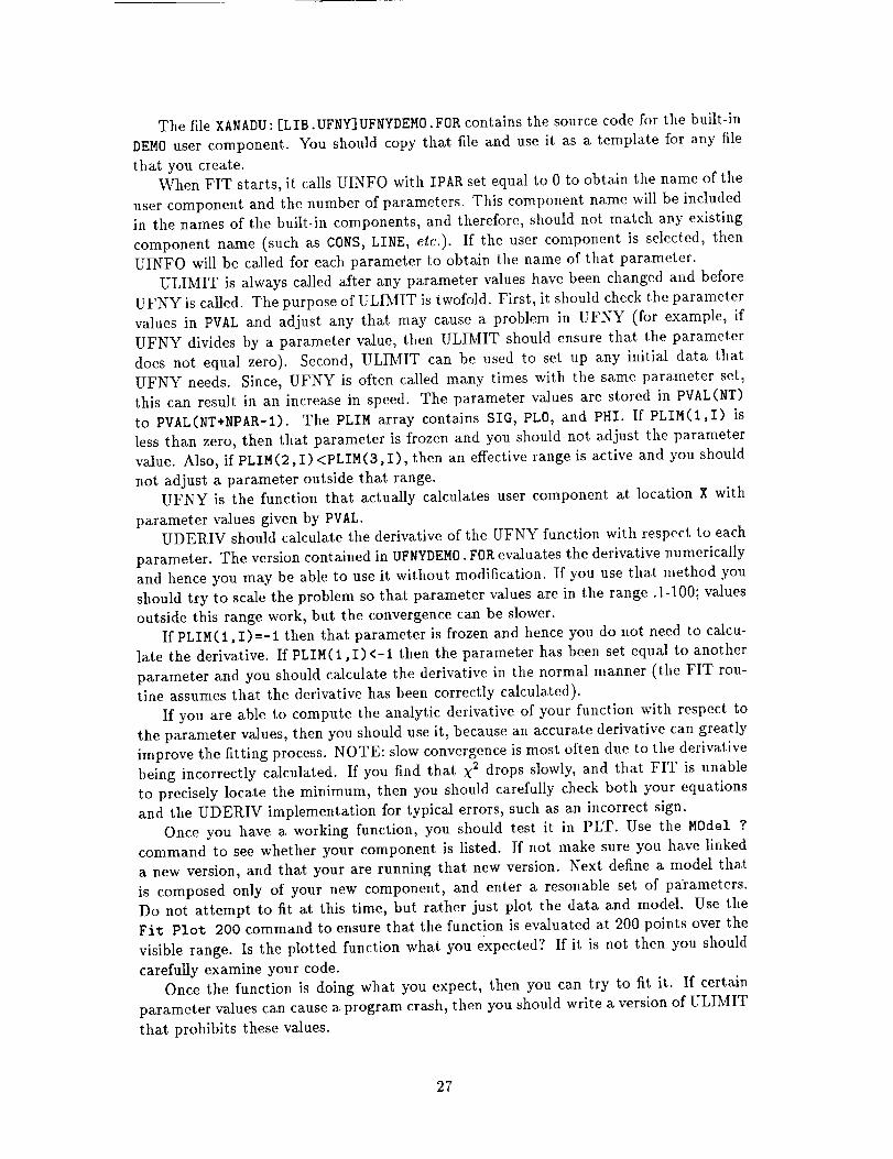
The file XANADU:[LIB .UFNY] UFNYDEMO.FOR contains the source code for the built-in
DEMOuser component. You should copy that file and use it as a template for any file
that you create.
When FIT starts, it calls UINFO with IPAR set equal to 0 to obtain the name of the
user component and the number of parameters. This component name will be included
in the names of the built-in components, and therefore, should not match any existing
component name (such as CONS, LINE, etc.). If the user component is selected, then
UINFO will be called for each parameter to obtain the name of that parameter.
ULIMIT is always called after any parameter values have been changed and before
UFNY is called. The purpose of ULIMIT is twofold. First, it should check the parameter
values in PVAL and adjust any that may cause a problem in UFNY (for example, if
UFNY divides by a parameter vMue, then ULIMIT should ensure that the parameter
does not equal zero). Second, ULIMIT can be used to set up any initial data that
UFNY needs. Since, UFNY is often called many times with the same parameter set,
this can result in an increase in speed. The parameter values are stored in PVAL(NT)
to PVAL(NT+NPAR-1). The PLIM array contains SIG, PL0, and PHI. If PLIM(1,I) is
less than zero, then that parameter is frozen and you should not adjust the parameter
value. Also, if PLIM(2 ,I)<PLIM(3, I), then an effective range is active and you should
not adjust a parameter outside that range.
UFNY is the function that actually calculates user component at location X with
parameter values given by PVAL.
UDERIV should calculate the derivative of the UFNY function with respect to each
parameter. The version contained in UFNYDEM0.FOR evaluates the derivative numerically
and hence you may be able to use it without modification. If you use that method you
should try to scale the problem so that parameter values are in the range .1-100; values
outside this range work, but the convergence can be slower.
If PLIM(1 ,I)=-I then that parameter is frozen and hence you do not need to calcu-
late the derivative. If PLIM (1, I)<-1 then the parameter has been set equal to another
parameter and you should calculate the derivative in the normal manner (the FIT rou-tine assumes that the derivative has been correctly calculated).
If you are able to compute the analytic derivative of your function with respect to
the parameter values, then you should use it, because an accurate derivative can greatly
improve the fitting process. NOTE: slow convergence is most often due to the derivative
being incorrectly calculated. If you find that X 2 drops slowly, and that FIT is unable
to precisely locate the minimum, then you should carefully check both your equations
and the UDERIV implementation for typical errors, such as an incorrect sign.
Once you have a working function, you should test it in PLT. Use the MOdel ?
command to see whether your component is listed. If not make sure you have linked
a new version, and that your are running that new version. Next define a model that
is composed only of your new component, and enter a resonable set of parameters.
Do not attempt to fit at this time, but rather just plot the data and model. Use the
Fit Plot 200 command to ensure that the function is evaluated at 200 points over the
visible range. Is the plotted function what you expected? If it is not then you should
carefully examine your code.
Once the function is doing what you expect, then you can try to fit it. If certain
parameter values can cause a program crash, then you should write a version of ULIMIT
that prohibits these values.
27

28
Chapter 7
COD
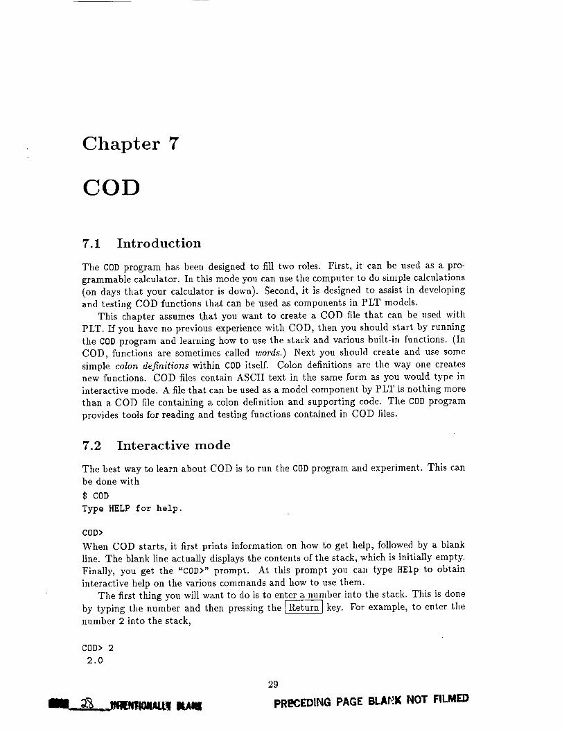
7.1 Introduction
The COD program has been designed to fill two roles. First, it can be used as a pro-
grammable calculator. In this mode you can use the computer to do simple calculations
(on days that your calculator is down). Second, it is designed to assist in developingand testing COD functions that can be used as components in PLT models.
This chapter assumes that you want to create a COD file that can be used with
PLT. If you have no previous experience with COD, then you should start by running
the ¢0D program and learning how to use the stack and various built-in functions. (In
COD, functions are sometimes called words.) Next you should create and use some
simple colon definitions within C0D itself. Colon definitions are the way one createsnew functions. COD files contain ASCII text in the same form as you would type in
interactive mode. A file that can be used as a model component by PLT is nothing more
than a COD file containing a colon definition and supporting code. The COD program
provides tools for reading and testing functions contained in COD files.
7.2 Interactive mode
The best way tolearn about COD isto run the ¢0D program and experiment. This canbe done with
$ COD
Type HELP for help.
COD>
When COD starts, it first prints information on how to get help, followed by a blank
line. The blank line actually displays the contents of the stack, which is initially empty.
Fina_y, you get the "COD>" prompt. At this prompt you can type HElp to obtain
interactive help on the various commands and how to use them.
The first thing you will want to do is to enter a number into the stack. This is done
by typing the number and then pressing the _Return_ key. For example, to enter the
number 2 into the stack,
COD> 2
2.0
amum_29
PRECEDING PAGE BLAI'_!K NOT FILMED

COD echos the stack and then returns the COD prompt (in this documentation the
final prompt is not shown). To execute a simple mathematical function, enter all the
numbers required by the function and then the function itself. The following sequence
shows how to multiply the previously entered 2 by the number 3 to obtain 2.3:
2.0
COD> 3
2.0 3.0COD> *6.0
With COD it is not necessary to enter one token (number or function) per line. Tokens
may be entered, separated by spaces, on a single line. Hence, to divide the result of the
previous calculation by 0.5, enter
6.0
COD> .5 /
12.0
COD contains several commands to manipulate the stack. Thus SWap will swap the top
two numbers on the stack, and DUP will duplicate the top number on the stack. When
using COD interactively, you will sometimes wish to clear out the stack. The can be
done using the ABOrt command. Thus,
12.0
COD> ABOrt
and the blank line indicating an empty stack will again appear just before the fol-
lowing COD prompt. There are a large number of built-in COD functions. To ob-
tain a list of the functions, you may use the List Dictionary command. If you
see a function and would like more information on what it does, you should use the
HElp Dictionary command. For a complete list of built-in COD commands, consult
Appendix A.
7.3 Colon definitions
When running COD interactively, it is sometimes necessary to enter the same sequenceof tokens several times. For such cases, you should create a colon definition that contains
the sequence. A colon definition consists of a colon : , followed by the function name,
followed by the sequence of COD functions that you wish to execute when the function
name is typed, and terminated with a semi-colon ; . For example, although there is
no built-in COD function to square a number, you can create one with
COD> : X2 DUP * ;
which will have the effect of multiplying the top number on the stack by itself. After
you have defined X2, it may be used in exactly the same way as any built-in function;
thus,
COD> 3.0 X2
9.0
A previously-defined colon function may be used in the definition of a new colon function.
An X3 function, for example, can be constructed from the X2 function with
3O
COD> : X3 DUP X2 * ;
9.0
COD> 3.0 X3
9.0 27.0
The name of a colon function is not allowed to match the name of any built-in function
or other colon function. Hence, a colon function cannot be used to redefine the action
of any existing COD keyword.
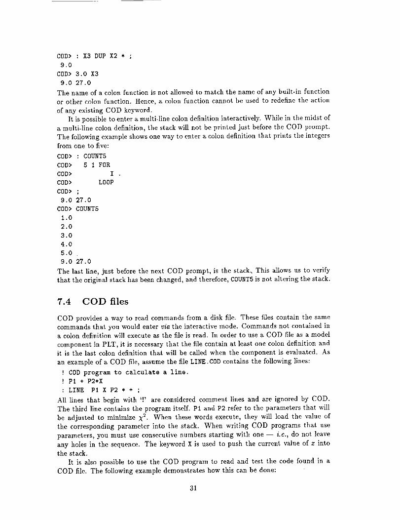
It is possible to enter a multi-line colon definition interactively. While in the midst of
a multi-line colon definition, the stack will not be printed just before the COD prompt.
The following example shows one way to enter a colon definition that prints the integers
from one to five:
COD> : COUNT5
COD> 5 I FOR
COD> I
COD> LOOP
COD> ;
9.0 27.0
COD> COUNT5
1.0
2.0
3.0
4.0
5.0
9.0 27.0
The last line, just before the next COD prompt, is the stack_ This allows us to verify
that the original stack has been changed, and therefore, C0UNT5 is not altering the stack.
7.4 COD files
COD provides a way to read commands from a disk file. These files contain the same
commands that you would enter via the interactive mode. Commands not contained in
a colon definition will execute as the file is read. In order to use a COD file as a model
component in PLT, it is necessary that the file contain at least one colon definition and
it is the last colon definition that will be called when the component is evaluated. As
an example of a COD file, assume the file LINE.COD contains the following lines:
! COD program to calculate a line.
! Pl + P2*X
: LINE P1 X P2 * + ;
All lines that begin with '!' are considered comment lines and are ignored by COD.
The third line contains the program itself. P1 and P2 refer to the parameters that will
be adjusted to minimize X 2. When these words execute, they will load the value of
the corresponding parameter into the stack. When writing COD programs that use
parameters, you must use consecutive numbers starting with one -- i.e., do not leave
any holes in the sequence. The keyword X is used to push the current value of x into
the stack.
It is a/so possible to use the COD program to read and test the code found in a
COD file. The following example demonstrates how this can be done:
31
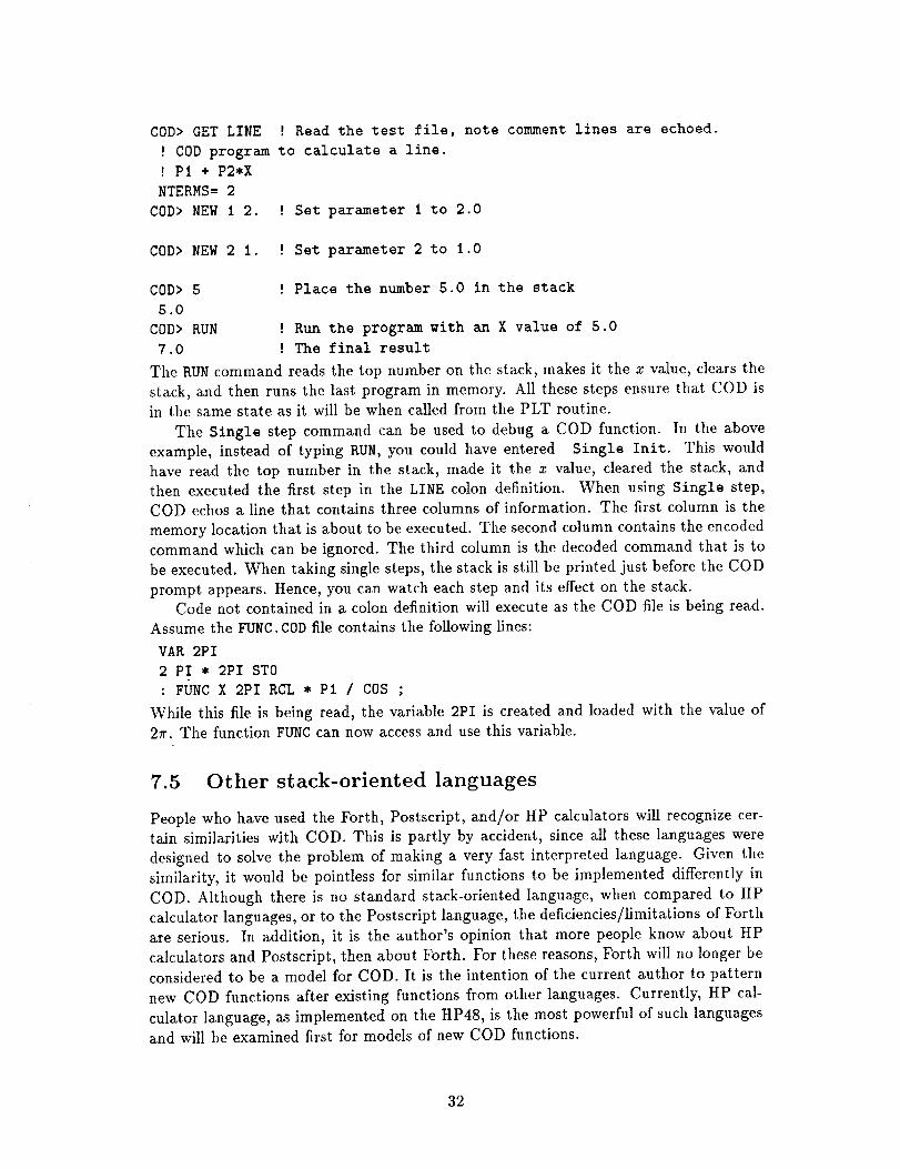
COD> GET LINE ! Read the test file, note comment lines are echoed.
a COD program to calculate a line.
i PI + P2*X
NTERMS= 2
COD> NEW i 2. ! Set parameter i to 2.0
COD> NEW 2 1. ! Set parameter 2 to 1.0
COD> 5 ! Place the number 5.0 in the stack
5.0
COD> RUN ' Run the program with an X value of 5.0
7.0 ! The final result
The RUN command reads the top number on the stack, makes itthe x value, clears the
stack, and then runs the last program in memory. All these steps ensure that COD is
in the same state as itwill be when calledfrom the PLT routine.
The Single step command can be used to debug a COD function. In the above
example, instead of typing RUN, you could have entered Single Init. This would
have read the top number in the stack, made it the x value, cleared the stack, and
then executed the firststep in the LINE colon definition. When using Single step,
COD echos a line that contains three columns of information. The firstcolumn isthe
memory location that isabout to be executed. The second column contains the encoded
command which can be ignored. The third column isthe decoded command that is to
be executed. V, rhen taking single steps, the stack is still be printed just before the COD
prompt appears. Hence, you can watch each step and its effect on the stack.Code not contained in _ colon definition will execute as the COD file is being read.
Assume the FUNC. COD file contains the following lines:
VAR 2PI
2 PI * 2PI STO
: FUNC X 2PI RCL * Pl / COS ;
While this file is being read, the variable 2PI is created and loaded with the value of
2_r. The function FUNC can now access and use this variable.
7.5 Other stack-oriented languages
People who have used the Forth, Postscript, and/or HP calculators will recognize cer-
tain similarities with COD. This is partly by accident, since all these languages were
designed to solve the problem of making a very fast interpreted language. Given the
similarity, it would be pointless for similar functions to be implemented differently in
COD. Although there is no standard stack-oriented language, when compared to HP
calculator languages, or to the Postscript language, the deficiencies/limitations of Forth
are serious. In addition, it is the author's opinion that more people know about HP
calculators and Postscript, then about Forth. For these reasons, Forth will no longer be
considered to be a model for COD. It is the intention of the current author to pattern
new COD functions after existing functions from other languages. Currently, HP cal-
culator language, as implemented on the HP48, is the most powerful of such languages
and will be examined first for models of new COD functions.
32

Appendix A
COD Command summary
Multiply the top two numbers in the stack.
Example:
5.0 2.0
COD> *
I0.0
+
Add the top two numbers in the stack.
Example:
5.0 2.0
COD> +
7.0
+LOOP
Terminate a COD FOR loop. When this statement executes, the number at the top of
• the stack is added to the current index. The loop terminates when the index passes the
limit value. The +LOOP statement allows for loops in which the index value can either
increase or decrease. This word can only be used in colon definitions.
Example:
COD> : TMP 0 2 FOR I -I +LOOP ;
COD> TMP
2.0
1.0
0.0
COD> : DOUBLE I00 I F0R I . I +LOOP ;
33

COD> DOUBLE
1.0
2.0
4.0
8.0
16.0
32.0
64.0
+STO
Add the previous number to the number stored at the address given at the top of the
stack. Although it is easy to determine the address associated with a given variable,
and hence use that address directly, it is advisable always to use a variable name to
load an address into the stack before using +ST0.
Example:
0.0
COD> VAR TMP 5 TMP STO TMP RCL
0.0 5.0
COD> TMP +STO
0.0
COD> TMP RCL
0.0 I0.0
Subtract the top two numbers in the stack.
Example:
5.0 2.0
COD> -
3.0
Print the number at the top of the stack, and decrement stack pointer by one. The
sequence "DUP ." can be inserted anywhere into COD functions to print the number at
the top of the stack. This may help you figure out what the function is doing.
Example:
1.0 2.0 3.0 4.0 5.0
COD>
5.0
1.0 2.0 3.0 4.0
34
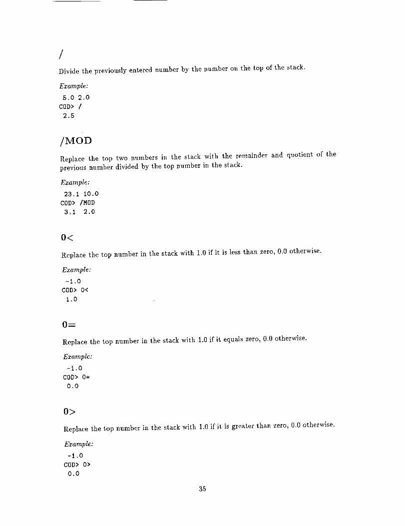
/Divide the previously entered number by the number on the top of the stack.
Example:
5.0 2.0
COD> /
2.5
/MOD
Replace the top two numbers in the stack with the remainder and quotient of the
previous number divided by the top number in the stack.
Example:
23.1 10.0
COD> /MOD
3.1 2.0
O<
Replace the top number in the stack with 1.0 if it is less than zero, 0.0 otherwise.
Example:
-1.0
COD> 0<
1.0
Replace the top number in the stack with 1.0 if it equals zero, 0.0 otherwise.
Example:
-1.0
COD> 0=
0.0
0>
Replace the top number in the stack with 1.0 if it is greater than zero, 0.0 otherwise.
Example:
-i .0
COD> O>
0.0
35

1+
Add one to the number at the top of the stack.
Example:
3.0 5.0
COD> I+
3.0 6.0
B
Subtract one from the number at the top of the stack.
Example:
3.0 5.0
COD> 1-
3.0 4.0
i/
Compute the inverse of the top number in the stack.
Example:
5.0 2.0
COD> I/
5.0 0.50
2+
Add two to the number at the top of the stack.
Example:
3.0 5.0
COD> 2+
3.0 7.0
2_
Subtract two from the number at the top of the stack.
Example:
3.0 5.0
COD> 2-
3.0 3.0
36
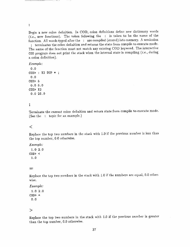
Begina newcolondefinition. In COD, colondefinitionsdefinenew dictionarywords(i.e., new functions). The token following the • is taken to be the nameof thefunction. All wordstypedafterthe : arecompiled(stored)intomemory.A semicolon
; terminatesthe colondefinitionandreturnsthe statefromcompileto executemode.The nameof thefunctionmust not matchanyexistingCODkeyword.Theinteractive¢0Dprogramdoesnot print the stackwhenthe internal stateis compiling(i.e., duringa colondefinition).
Example:
0.0
COD> : X2 DUP * ;
0.0
COD> 5
0.0 5.0
COD> X2
0.0 25.0
Terminate the current colon definition and return state from compile to execute mode.
(See the : topic for an example.)
<
Replace the top two numbers in the stack with 1.0 if the previous number is less than
the top number, 0.0 otherwise.
Example:
1.0 2.0
COD> <
1.0
w
Replace the top two numbers in the stack with 1.0 if the numbers are equal, 0.0 other-
wise.
Example:
1.0 2.0
COD> =
0.0
>
Replace the top two numbers in the stack with 1.0 if the previous number is greater
than the top number, 0.0 otherwise.
37
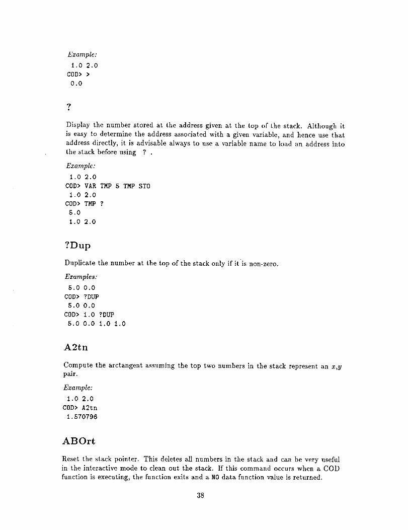
Example:
i.O 2.0
COD> >
0.0
?
Display the number stored at the address given at the top of the stack. Although it
is easy to determine the address associated with a given variable, and hence use that
address directly, it is advisable always to use a variable name to load an address into
the stack before using
Example:
1.0 2.0
COD> VAR TMP 5 TMP STO
1.0 2.0
COD> TMP ?
5.0
1.0 2.0
?Dup
Duplicate the number at the top of the stack only if it is non-zero.
Examples:
5.0 0.0
COD> ?DUP
5.0 0.0
COD> 1.0 ?DUP
5.0 0.0 1.0 1.0
A2tn
Compute the arctangent assuming the top two numbers in the stack represent an x,ypair.
Example:
1.0 2.0
COD> A2_n
1.570796
ABOrt
Reset the stack pointer. This deletes all numbers in the stack and can be very useful
in the interactive mode to clean out the stack. If this command occurs when a COD
function is executing, the function exits and a NO data function value is returned.
38

ABS
Take the absolute value of the top number in the stack.
Example:
5.0 -2.0
COD> ABS
5.0 2.0
ACos
Computer the arccosine (in radians) of the top number in the stack.
Example:
5.0 0.5
COD> ACos
5.0 1.047198
ALog
Compute 10. raised to the power of the top number in the stack.
Example:
5.0 2.0
COD> ALog
5.0 100.0
ASin
Compute the arcsine (in radians) of the top number in the stack.
Example:
5.0 0.5
COD> ASin
5.0 0.5235988
ATan
Compute the arctangent (in radians) of the top number in the stack.
Example:
5.0 0.5
COD> ATan
5.0 0.4636476
BEGIN
Begin a BEGIN...UNTIL or a BEGIN...WHILE...REPEAT structure. See either the UNTIL
or WHILE topics for examples of use. This word can only be used in colon definitions.
39

COS
Compute the cosine of the top number (in radians) in the stack.
Example:
5.0 0.5
COD> COS
S.O 0.8775826
DDms
Convert a number in decima] degrees to the _rm DDDMMSS.S .
Example:
12.5
COD> DDms
123000.0
DEPth
Leave the number of values contained in the stack (not counting the result).
Example:
5.0 4.0
COD> DEP
5.0 4.0 2.0
DMsd
Convert a number oftheformDDDMMSS.S to decimal degrees.
Example:
123000.0
COD> DMsd
12.5
DRop
Drop the stack pointer so that the number at the top of the stack is ]ost.
Example:
5.0 4.0
COD> DRop
5.0
4O

DTor
Convert decimal degrees to radians.
Example:
5.0 90.0
COD> DTor
5.0 1.570796
DUP
Duplicate the number on the top of the stack (equivalent to
Example:
5.0 2.0
COD> DUP
5.0 2.0 2.0
i PICK).
ELSE
If the condition was false when the IF statement executed, then transfer control to the
first statement following the ELSE. If the condition was true, then the function executes
code down to the ELSE statement and then skips to the first statement following the
THEN statement. This statement must be preceded by an IF statement: This word can
only be used in colon definitions. See the IF topic for an example.
EXIT
Immediately terminate the current colon function. Since the stack is unaffected, check
to verify that the stack is left in the same state no matter how the colon function is
terminated (otherwise obscure and nasty bugs result). This word can only be used in
colon definitions.
EXP
Compute the exponential of the top number in the stack.
Example:
5.0 1.0
COD> EXP
5.0 2.718282
FOR
Set up a FOR...LOOP or a FOR...+LOOP structure using the top two numbers in the stack
to denote the range. The index for the FOR loop is an INTEGER*2, hence the maximum
value is 32767. This word can only be used in colon definitions.
Example:
41
COD> : TMP 4 1 FOR I . LOOP ;
C0D> TMP
1.0
2.0
3.0
4.0
Warning to people who know Forth: The COD FOR statement is similar to the Forth D0
statement; however, there is an important difference concerning the two numbers that
precede the FOR. In COD, these represent the upper and lower index values, respectively;
in Forth, the first number is one greater than the upper index value.
HCos
Compute the hyperbolic cosine of the top number in the stack.
Example:
5.0 0.5
COD> HCos
5.0 1.127626
HSin
Compute the hyperbolic sine of the top number in the stack.
Example:
5.0 0.5
COD> HSin
5.0 0.5210953
HTan
Compute the hyperbolic tangent of the top number in the stack.
Example:
5.0 0.5
COD> HTan
5.0 0.4621172
I
Push the index value of the innermost FOR loop onto the stack. This statement can only
be used inside FOR loops inside a colon definition. See the FOR topic for an example ofuse.
42
IF
If the condition is true, execute statements up to the corresponding ELSE or THEN state-
ment. If the condition is false, pass control to the first statement following the ELSE if it
exists, otherwise to the first statement following the THEN. IF structures can be nested.
This word can only be used in colon definitions.
Example:
X 1<
IF
! do these statements if X<l
THEN
X i >
IF
do these statements if X>I
ELSE
do these statements if X<=I
THEN
INT
Compute the integer portion of the top number in the stack.
Example:
5.0 0.9
COD> INT
5.0 0.0
J
Push the index value of the next outer FOR loop onto the stack.
only be used inside F0R loops inside a c_on definition.
Example:
COD> : TMP 2 i FOR
COD> 5 4 FOR
COD> J . LOOP LOOP ;
This statement can
COD> TMP
1.0
1.0
2.0
2.0
LEAVE
Cause an immediate exit from the current loop. No statements from the LEAVE state-
ment to the loop terminator are executed. This statement resembles the Fortran 8x
43

EXIT statement.LEAVEcanonly beusedinsideFORloopsinsidea colondefinition.
LN
Take the natural logarithm of the top number in the stack.
Example:
5.0 2.0
COD> LN
5.00. 693i472
LOG
Take the base-10 logarithm of the top number in the stack.
Example:
5.0 2.0
COD> LOG
5.0 0.3010300
LOOP
Terminate a COD FOR loop. When this statement executes, one is added to the current
index value. If the current index is less than or equal to the maximum index, then
control is transferred to the first statement following the corresponding FOR statement.
Otherwise, control passes to the statement following the LOOP statement. This word
can only be used in colon definitions. See the FOR topic for an example of use.
MAX
Replace the top two numbers in the stack with the maximum of the two numbers.
Example:
1.0 3.0 5.0
COD> MAX
1.0 5.0
MIN
Replace the top two numbers in the stack with the minimum of the two numbers.
Example:
1.0 3.0 5.0
COD> MIN
1.0 3.0
44

MOD
Compute the vMue of the previous number modulo the top number in the stack.
Example:
2.03.0
COD> MOD
2.0
COD> ABO 3.0 3.0
3.03.0
COD> MOD
0.0
NEG
Negate the top number in the stack.
Example:
5.0 2.0
COD> NEG
5.0 -2.0
NInt
Compute the nearest integer to the top number in the stack.
Example:
5.0 0.9
COD> NInt
5.0 1.0
NOT
Replace the top number in the stack with 1.0 ifitiszero, 0.0 otherwise.
Example:
1.0
COD> NOT
0.0
OVer
Duplicate the second number on the stack (equivalent to
Example:
5.0 4.0
COD> OVER
5.0 4.0 5.0
2 picK).
45

PI
Push the value of _" into the stack.
Example:
5.0
COD> PI
5.0 3. 141593
PICK
Duplicate the nth number on the stack (not counting n itself), where n is the top number
on the stack. Note: 1 PICK does the same thing as DUP, and 2 PICK does the same
thing as OVER.
Example:
100. 200. 300. 400.
COD> 3 PICK
100. 200. 300. 400. 200.
RCL
Replace the address at the top of the stack with the number at that address. See the
STO topic for an example of how RCL isused.
REPEAT
Terminate a BEGIN...WHILE...REPEAT loop. When this statement executes, control is
always passed to the first statement following the BEGIN statement. This word can only
be used in colon definitions. See the WHILE topic for an example of use.
ROLL
Rotate the nth number (not counting n itself) to the top of the stack, where n is the
top number in the stack. Note: 2 ROLL does the same thing as SWAP, and 3 ROLL
does the same thing as ROT; and n must be greater than 1.0.
Example:
100. 200. 300. 400.
COD> 4 ROLL
200. 300. 400. 100.
ROT
Rotate the third number to the top of the stack (equivalent to
Example:
3 ROLL).
46

iO0. 200. 300. 400.COD> ROT
iO0. 300. 400. 200.
RTod
Convert radians to decimal degrees.
Example:
5.0 1.0
COD> RTod
5.0 57. 29578
SIN
Compute the sine of the top number (in radians) in the stack.
Example:
5.0 0.5
COD> SIN
5.0 0.4794255
SQrt
Compute the square-root of the top number in the stack.
Example:
5.0 2.0
COD> SQrt
5.0 1.414214
STO
Store the previous number at the address given at the top of the stack. Although it
is easy to determine the address associated with a given variable, and hence use that
address directly, it is advisable always to use a variable name to load an address into
the stack before using ST{3.
Example:
1.0
COD> VAR TMP
i.O
COD> 5 TMP STO
i.O
COD> TMP RCL
1.0 5.0
47

SWap
Swap the top two numbers on the stack (equivalent to
Example:
5.0 2.0
COD> SWap
2.0 5.0
2 ROLL).
TAN
Compute the tangent of the top number (in radians) in the stack.
Example:
5.0 0.5
COD> TAN
5.0 0.546302S
THEN
Terminate an IF structure. This word can only be used in colon definitions. See the IF
topic for an example of use.
TSig
Transfer the sign of the top number in the stack to the absolute value of the previous
number.
Example:
2.0 -5.0
COD> TSig
-2.0
UNTIL
Terminate a BEGIN...UNTIL block. UNTIL pops one number off the stack. If that
number is false (=0.0), the function jumps back to the first statement following the
BEGIN statement. Otherwise execution continues with the statement following the UNTIL
statement. This word can only be used in colon definitions.
Example:
COD> VARY ' Create variable Y
COD> : TEST 2 Y STO ' Initialize Y to 2
COD> BEGIN
COD> Y RCL ' Print the value of Y
COD> Y RCL DUP * Y STO ! Square it and store new value
COD> Y RCL I.EIO > ' Test condition
48
COD>UNTIL ;
COD> TEST
2.0
4.0
16.0
256.0
4.2949673E+9
VAR
Define the following token to be a new variable name. The variable name is not allowed
to match any existing COD keyword. When that variable is used in the future, it will
cause the address of that variable to be loaded into the stack (for use with a following
ST0 or RCL command).
Example:
0.0
COD> YAK 2PI 2 PI * 2PI STO
0.0
COD> 2PI RCL
0.0 6.283185
WHILE
The WHILE statement pops one number off the stack. If that number is true (# 0.0),
the statement following the WHILE will be executed. If the number is false, then control
passes to the first statement following the REPEAT statement. This statement can only
be used inside a BEGIN...WHILE...REPEAT loop in a colon definition.
Example:
COD> VARY ! Create variable Y
COD> : TEST 2 Y STO
COD> BEGIN
COD> Y RCL
COD> Y RCL I.EIO < WHILE
COD> Y RCL DUP * Y STO
COD> REPEAT ;
! Initialize Y to 2
' Print the value of Y
! Recall number and test for <I.EIO
! Square and store new value
COD> TEST
2.0
4.0
16.0
256.0
4. 2949673E+9
1.8446744E+ 19
49
X
Push the current X value into the stack.
A
Raise the previously entered number to the power given by the top number in the stack.
Example:
5.0 2.0COD> -
25.0
5O
Appendix B
PLT Command summary
CLear
CLear
Immediately clear the current plot device.
COlor
COlor [#] 0NIOFf [glist]
The first(optional) number allows you to reset the default color index for the plot
groups specifiedin [glist]. Ifthis number isomitted, then the default color index is
not changed. COlor OFf turns off the plotting of all plot groups specified;C01or ON
turns the plotting back on. If [glist] isomitted then allplot groups are affected.
COlor M0del #
Plot the model using color index #.
Color # 0N Grid
Use the color index specified by # when plotting the Grid in the currently active window.
COlor ?
Generate a listof possible color indices and their default color representations.
Examples:
PLT> COlor 0Ff 1,2,3
PLT> COlor 0N 2
PLT> COlor 5 ON 3
! Suppress plotting of groups I, 2,
a Turn on plotting of group 2
' Use color 5 when plotting group 3
and 3
51
CONtour
CONtour [#] ?]COlor list[LEvel list]LStyle list[LWidth list]0Ff
This command enables PLT to produce a contour plot. Itisstillexperimental, and so the
syntax could change. IfPLT isdisplaying contours, then you can use the SHow Contour
command to display the PLT commands that were used to generate that PLT.
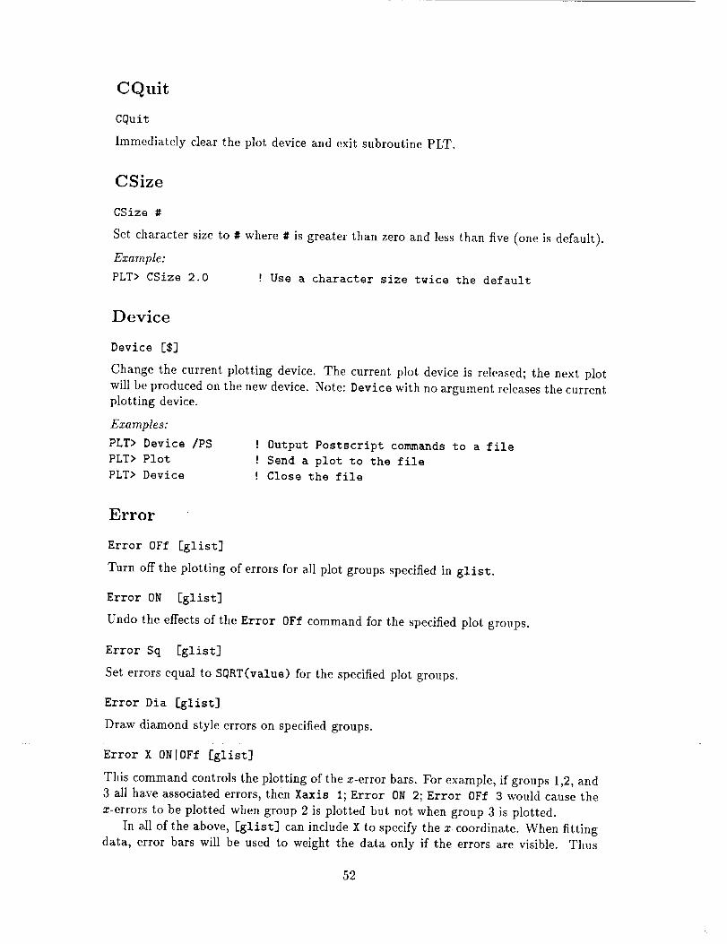
CQuit
CQuit
Immediately clear the plot device and exit subroutine PLT.
CSize
CSize #
Set character size to # where # is greater than zero and less than five (one is default).
Example:
PLT> CSize 2.0 ! Use a character size twice the default
Device
Device [$]
Change the current plotting device. The current plot device is released; the next plot
will be produced on the new device. Note: Device with no argument releases the current
plotting device.
Examples:
PLT> Device /PS
PLT> Plot
PLT> Device
! Output Postscript commands to a file
! Send a plot to the file
! Close the file
Error
Error OFf [glist]
Turn off the plotting of errors for all plot groups specified in glist.
Error ON [glist]
Undo the effectsof the Error OFf command for the specified plot groups.
Error Sq [glist]
Set errors equal to SQRT(value) for the specifiedplot groups.
Error Dia [glist]
Draw diamond style errors on specifiedgroups.
Error X ON[OFf [glist]
This command controls the plotting of the x-error bars. For example, ifgroups 1,2,and
3 all have associated errors,then Xaxis I;Error ON 2; Error OFf 3 would cause the
x-errors to be plotted when group 2 isplotted but not when group 3 isplotted.
In all of the above, [glist] can include X to specify the x-coordinate. When fitting
data, error bars will be used to weight the data only if the errors are visible. Thus
52

Error OFf followed by Fit will produce an unweighted fit.
y-errors are used to weight the data.
Examples:
PLT> Error 0Ff 1,2,3 !
PLT> Error Dia 2
PLT> Error 0N
PLT> SKip Sing
PLT> Error OFF X
Also, note that only the
Turn off errors for groups i, 2, and 3
Plot diamond errors on plot group 2
Plot errors for all plot groups
Turn on the _skip' mode
Suppress plotting of errors on X-axis
EXit
EXit
Emt subroutine PLT.
Fit
Fit [#] [Iterate #]
Cause PLT to call the fitting routine to search for the best fitting parameters for the
model specified with the MOdel command. The first optional number is the plot group to
fit. If this number is omitted, then Fit will continue to fit the previous group that you
were fitting if that plot group is still visible. For the first use of Fit or if the plot group
has been COlored OFf then Fit will default to fitting the lowest numbered group which
is visible. LAbel PArm command controls whether the model parameters are plotted on
the right side of the plot. Fitting continues until AX 2 is less than 0.05. As a default,
you will be prompted to continue fitting every 10 iterations. If you wish to increase the
number of iterations without being prompted, then use the Fit Iterate [#]. Thus,
Fit I 100, would allow the program to try up to 100 iterations before you would be
prompted again.
Fit ON [#]
Cause the current model to be plotted on group #. If # is omitted, the model will be
plotted on the plot group that was most recently fitted.
Fit 0Ff
Cause the model to no longer be plotted.
Fit Plot #
Control where the model isevaluated when itplotted. If# isgreater than zero, then the
model isevaluated at # points between the current x-scale Minimum and Maximum. If
# is less than 0, then the model is evaluated at ABS(#) points between the Data Min
and Data Max -- i.e.,no extrapolation is allowed. If # equals 0, then the model is
evaluated at the values of the data points. (This isthe default).
Fit Stat Chi]Ml #
Set the default fittingstatisticto either X 2 or maximum likelihood. For example,
Fit Stat M 2 would vary the fitparameter to minimize the likelihood function when
compared with plot group 2.
53
FNy
FNy #
Return the value ofthe current M0delfunction atlocation #.
Example:
PLT> MOdel LINR CONS ! Define a straight line
i, LI: VAL(1.00), SIS( 0.00 ), PLO(0.00), PHI( 0.00)?
2. ! Set slope of line equal to 2
2, CO: VAL(1.00), SIG( 0.00 ), PLO(0.00), PHI( 0.00)?
3. ! Set intercept of line equal to 3
PLT> FNY 3 ! Evaluate function at x=3.0
12.0 ! The result
FOnt
F0nt $
Set the default to the font specified by the character string. (Default is Simple font).
FOnt ?
List possible fonts.
Example:
PLT> Font Roman ! Use the Roman font
FReeze
FReeze [plist]
Can only be used after a model has been defined. This command causes all parameters
listed in [plist] to be frozen, which means the parameter value is not allowed to vary
during a Fit.
Examples:
PLT> FReeze 2 ! Freeze the value of parameter 2
PLT> FReeze 3..5 9 ! Freeze the values of parameters 3 through 5 and 9
GAp
GAp #
Control the size of the gap between the edge of the plot and the data extreme, when
using the default scale. The effect of the GAp command can only be seen when you
reset the default scale with R, R X, or R Y (all with no arguments). The default gap
is 0.025 which will leave a 2.5 percent margin around the edge. The size of the gap
in world coordinates, depends on whether the data are being plotted on a logarithmic
scale. Therefore, if you wish to use a default scale with a logarithmic scale, you should
first issue the L0g and GAp commands and then use the Rescale command to reset the
default scale.
54
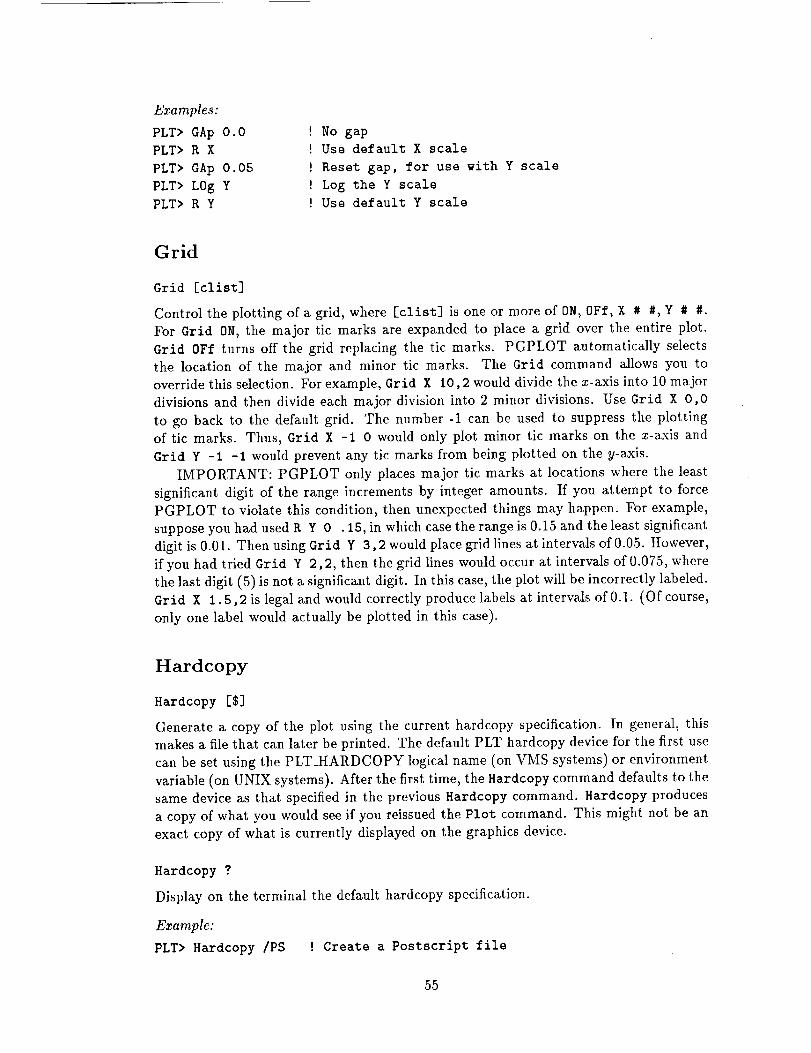
Examples:
PLT> GAp 0.0
PLT> R X
PLT> GAp 0.05
PLT> LOg Y
PLT> R Y
' No gap
! Use default X scale
! Reset gap, for use with Y scale
! Log the Y scale
! Use default Y scale
Grid
Grid [clist]
Control the plotting of a grid, where [clist] isone or more of ON, 0Ff, X # #, Y # #.
For Grid 0N, the major tic marks are expanded to place a grid over the entire plot.
Grid 0Ff turns off the grid replacing the tic marks. PGPLOT automatically selects
the location of the major and minor tic marks. The Grid command allows you to
override this selection. For example, Grid X 10,2 would divide the x-axis into 10 major
divisions and then divide each major division into 2 minor divisions. Use Grid X 0,0
to go back to the default grid. The number -1 can be used to suppress the plotting
of tic marks. Thus, Grid X -1 0 would only plot minor tic marks on the x-axis and
Grid Y -1 -1 would prevent any tic marks from being plotted on the y-axis.
IMPORTANT: PGPLOT only places major tic marks at locations where the least
significant digit of the range increments by integer amounts. If you attempt to force
PGPLOT to violate this condition, then unexpected things may happen. For example,
suppose you had used R Y 0 . 15, in which case the range is 0.15 and the least significant
digit is 0.01. Then using Grid Y 3,2 would place grid lines at intervals of 0.05. However,
if you had tried Grid Y 2,2, then the grid lines would occur at intervals of 0.075, where
the last digit (5) is not a significant digit. In this case, the plot will be incorrectly labeled.
Grid X 1.5,2 is legal and would correctly produce labels at intervals of 0.1. (Of course,
only one label would actually be plotted in this case).
Hardcopy
Hardcopy [$]
Generate a copy of the plot using the current hardcopy specification. In general, this
makes a file that can later be printed. The default PLT hardcopy device for the first use
can be set using the PLT_HARDCOPY logical name (on VMS systems) or environment
variable (on UNIX systems). After the first time, the Hardcopy command defaults to the
same device as that specified in the previous Hardcopy command. Hardcopy produces
a copy of what you would see if you reissued the Plot command. This might not be an
exact copy of what is currently displayed on the graphics device.
Hardcopy ?
Display on the terminal the default hardcopy specification.
Example:
PLT> Hardcopy /PS ! Create a Postscript file
55

HElp
HElp [pcommand]
Get help on the PLT command specified by [pcommand].
Imodel
Imodel # # [#]
Integrate the current model over the range specified by the firsttwo parameters. The
third (optional) argument is the number of steps. (Default is 100).
LAbel
LAbel X I Y ] Top ] 0X ] 0Y ] 0Top ] File J G# [label]
Place a label. The arguments X, Y, and Top would place a label on the x-axis, y-axis,
or the top of the plot. It is possible to place an additiona] line of text just outside
these locations by putting the letter '0' in front of these names. For example, 0T would
write a second label above the top label. Finally one can change the file name by using
LA File [name]. If you should at any time wish to delete a label, then just omit the
[label] from the command. The command LA G# label would associate a label with
a particular plot group. PLT will use the group label on either the x or y-axis if there
is no corresponding x or y label.
LAbel 0Ff
Suppress plotting of all text labels. (This speeds up the production of the plot on slow
devices).
LAbel ON
Undo the effectsof LAbel OFf.
LAbel NX]NY 0NIOFf [winlist]
where [winlist] is a list of windows. NX affects the plotting of the numeric labels
on the x-axis, NY on the y-axis. Thus LAbel NX OFF 1; LAbel NY OFF 1, will prevent
the plotting of the numeric labels in both the X and Y directions for the first window.
Note: there are 32 numbered labels, so using LAbel NX OF, followed by several LAbel #
commands will allow you to create labels consisting of text strings etc.
LAb P0S Y #
Allows the position of the y label(s) to be moved. The default position is LA P0S Y 2.0.
LAbel Rotate
Rotate numerical labels plotted on the y-axis. The default PGPLOT mode is to plot
the y-axis numerical labels in the vertical direction. LAbel Rotate will rotate these
labels so they are written in a horizontal direction. If you issue the command a second
time, then the labels will flip back to vertical in the next plot.
Ezamples:
56
PLT> LA F
PLT> LA T Test! Plot
PLT> LA T "Test! Plot"
' Delete the file name from the plot
! Top label is Test
! Top label is Test! Plot
LAbel Parm 0N
Display the parameter vMues, associated with the current model, on the right side of
the plot. (This is the default).
LAbel Parm 0Ff
Suppress the display of the parameter values on the right side of the plot.
LAbel # [clist] "string"
Allow a label to be placed anywhere on the existing graph. Here # is a number in
the range 1 to 32, [clist] is a list of subcommands that allow you to change various
attributes of the label, and "string" is the (optional) text. For example,
PLT> LAbel 1 Pos 2 2 "test"
will create label 1 at position (2,2) containing the message test.
LAbel # CEnter ToplCaplHalf lBAselBOttom
Control the vertical position of the text string. The default position is half, although
the use of the Line subcommand will override this.
LAbel # COlor #
Cause the label to be plotted with color index #. (Default is color index 1).
LAbel # CSize #
Cause the label to be plotted with character size #. (Default ischaracter size 1.0).
LAbel # Justify Left ]Center ]Right
Control justification of text string. (Default is to center justify).
LAbel # Line # [#]
Draw line at angle # (in degrees) from position to the label. If the second number is
specified, then it will be used as the length of the line in viewport units. (Default line
length is 0.08). If no number follows the Line command, then the line is turned off.
LAbel # LStyle #
Control the line style of the line plotted, when the Line subcommand is used. (Default
is 1).
LAbel # Marker #
Include marker # in the text line.The default willproduce a leftjustifiedstringjust to
the right of the marker. Ifyou then right justifythe string,then the string will appear
to the leftof the marker. In either case, the (x, y) position corresponds to the position
of the marker.
LAbel # MSize #
Use the specified marker size with plotting the specified numbered label.
LAbel # Position # #
57

Specify the (x,y) location of the string in world coordinates. When using the Line
subcommand, Position # # gives the (x, y) location of the position being 'pointed at'
with the text string at the other end. If the Marker subcommand is used, then # #
refers to the location of the marker. For other cases, # # is the location of the string.
The CEnter and Justify subcommands can later override how text is plotted relative
to a location. (The default location is (0,0)).
LAbel # Position Cursor
Display the cursor at the current default position. You can move the cursor to the
desired position using the standard (PGPLOT) cursor keys. Once at the location where
you want the label, press the space bar. The next time the plot is drawn, the label will
appear at the new location.
LAbel # Rotate #
Plot the label at an angle of # (degrees) relative to the x-axis. (Default angle is 0).
LAbel # YPos # #
Specify the (x, y) location of the string in viewport coordinates. When using the Line
subcommand, Position # # gives the (x, y) location of the position being 'pointed at'
with the text string at the other end. If the Marker subcommand is used, then # #
refers to the location of the marker. For other cases, # # is the location of the string.
The CEnter and Justify subcommands can later override how text is plotted relative
to a location.
LAbel # VPos Curs
Display the cursor at the current default position. You can move the cursor to the
desired position using the standard (PGPLOT) cursor keys. Once at the location where
you want the label, press the space bar. The next time the plot is drawn, the label will
appear at the new location.
Examples:
PLT> LAbel I "TEST"
PLT> LAbel I P I0 I0
PLT> LAbel I Line 90
PLT> LAbel i C0 3
PLT> LAbel I P i0 I0 Line 90 C0 3 "TEST"
PLT>
! Place the word TEST at location (0,0)
! TEST will now appear centered at (I0,i0)
! Draw a vertical line from the point (i0,I0) to
! the word TEST.
' Color line and word TEST green
! Does all the above in a
' single command
Line
Line 0N [glist]
Draw a line connecting all the points in each plot group specified in [glist].
Line 0Ff [glist]
Produce a scatter diagram by turning off the line for each plot group specified in
[glist].
58
Line Stepped [glist]
Produce a stepped-fine plot for each plot group specified in [glist].
Note: If you set Error OFf, MArker OFf, and Line OFf, then the line will still
appear. The only way to prevent data from being plotted is to use the COlor OFf
command.
Examples:
PLT> Line ON
PLT> Line OFf 1,3
PLT> Line Step 1,5
! Use a line for all groups
! Turn off the line for groups I and 3
! Plot groups i and 5 with a stepped line
LOCation
LOCation # [# [# [#]]]
The LOCation command allows you to control the location of the currently active win-
dow. The default location of all windows is 0. 0. 1. 1. which means that all windows
overlap and use the entire plotting surface. This command in combination with the
Window command allows great control over where the windows are plotted. Thus a
small window could be plotted inside a larger one. However, no attempt is made to
erase a plotting region, so overlapping windows could result in overlapping text.
Example: To create 4 windows in the 4 quadrants, use:
PLT> Window i
PLT> LOCation 0 .5 .5 I.
PLT> Window 2
PLT> LOCation .5 .5 i. i.
PLT> Window 3
PLT> LOCation 0. 0..5 .5
PLT> Window 4
PLT> LOCation .5 0. i..5
LOg
L0G XIYIX,Y 0NIOFf [winlist]
Controls whether a log scale is used when plotting in the windows specified in wJnlist.
Thus L0G Y 0Ff 2 3 4, would turn off the use of a log scale in the y direction in
windows 2 3 and 4. Also, LOG X,Y 0Ff 3 would turn off the log scale in both the x and
y directions when plotting in window 3.
LStyle
LStyle # [ON] [glist]
Change the default fine style for the plot groups specified in [glist]. The first number
is the style type.
LStyle # 0N Grid
59
Use the line style specified by # when plotting the grid in the currently active window.
LStyle ?
List possible Hne styles.
Examples:
PLT> LStyle 2 0N 3
PLT> LStyle 1
PLT> LStyle 5 ON 1,4
! Use line style 2 when plotting group 3
! Use solid line when plotting all groups
! Use line style 5 when plotting groups 1 and 4
LWidth
LWidth #
Set the fine width to the value #. AHowed values are 1 or greater. On some laser
printers, the default line width is very narrow and so, using thicker lines will enhance
the output quality.
Examples:
PLT> LWidth 3 ! Triple the default thickness of all lines
PLT> HArd /PS ! and make a hardcopy
MArker
MArker [#] ON [glist]
Turn on the plotting of polymarkers. The first(optiona/) number is the marker type;
ifomitted the default marker type will not be changed. If [glist] is omitted, then
markers will be used to plot all plot groups.
MArker Size # 0N [glist]
Changes the size of the markers when plotting the plot groups specified in [glist].
The sizecan range from 0.0 to 5.0, where 1.0 isthe default. Thus every plot group can
have a differentmarker size.
MArker OFf [glist]
Turn of[ the plotting of markers for all plot groups specified.
then markers will be removed from a/lgroups.
If [glist] is omitted,
MArker ?
Draw a table of all the PGPLOT markers on your current graphics device.
Examples:
PLT> MArk 19 0N 2
PLT> MArk OFF 2
PLT> MArk ON 2
PLT> MArk 0N
PLT> MArk Size 5
! Use marker 19 when plotting group 2
! No longer plot group 2 with a marker
! Use default marker when plotting group 2
' Use markers when plotting all plot groups
' Plot markers 5 times larger than default size
60

MOdel
MOdel ?
List all built-in model components.
M0del ©filename
Cause the model definition and parameters to be read from the file with name filename.
MOdel $
Use to define models. Any combination of model components can be added together.
For example, MOdel CONS LINR QUAD will add a constant term, a linear term, and a
quadratic term.
For each parameter required by the MOdel command, you will be prompted for four
numbers -- VAL, SIG, PL0, and PHI -- as described below. For each parameter, you
should enter an initial value for VAL; but you can usually default on the other three
numbers.
VAL: This is the actual value of the parameter. Although CURFIT will often find
the the best set of parameters to model the data, it never hurts to start it with
parameters near the expected best fit.
SIG: Any value of SIG>0 will not affect the outcome of Fit. After you fit the model,
SIG will contain the one-sigma curvature errors. This number is used by the
Uncertainty command to start a formal error determination. If the Uncertainty
command fails to converge because the original error estimate is wrong, sometimes
you can help the convergence by adjusting SIG to be a better estimate before using
Uncertainty. If you set SIG=-I, then the parameter is frozen such that CURFIT
is not allowed to change the parameter value while fitting. If you set SIG=-IPAR,
the next number (PL0) will default to 1, such that the current parameter value is
forced to equal the value of parameter IPAR. (Note: IPAR can not equal 1 or the
current parameter number). If you place a number (N) after SiS, this will force
the current parameter to be N times the specified parameter. (N defaults to 1.0.)
Example:
PLT> MOdel GAUS GAUS
i, GC: VAL(1.00), SIG( 0.00 ), PLO(0.00), PHI( 0.00)?
,-4,2
2, GW: VAL( 1.00), SIG( 0.00 ), PLO( 0.00), PHI( 0.00)?
3, GN: VAL(1.00), SIG( 0.00 ), PLO(0.00), PHI( 0.00)?
4, GC: VAL(1.00), SIG( 0.00 ),
3.
5, GW: VAL(1.00), SIG( 0.00 ),
PLO(0.00), PHI( 0.00)?
PLO(0.00), PHI( 0.00)?
6, GN: VAL( 1.00), SIG( 0.00 ), PLO( 0.00), PHI( 0.00)7
61

defines a model consisting of two gaussians, with the x values of the centers dif-
fering by a factor of 2. Although a value for parameter 1 was not entered, it will
be set to the vMue of 6 (2 times value of parameter 4). This relationship will be
maintained throughout a fit.
PL0, PHI: If SIG>0 and if PL0<PHI, the parameter value is constrained to lie within
the range PL0 to PHI. Note: If PL0 and PHI are the same (say equal to zero),
then the parameter will not be constrained in any way. In general, if you have
difficulty fitting some data, the best thing to do is to freeze some parameters near
to their expected values and then fit the reduced parameter set. When a good fit
has been found with the reduced set, thaw some of the parameters and refit. If
this method does not work, then you may be forced to use PL0 and PHI to limit
certain parameters to a meaningful range.
QDP/PLT currently supplies the model components defined below, which may be
combined into multi-component models:
MOdel CONS
Select a model with a constant component:
FNY=FNY+CO.
MOdel LINR
Select a model with a Hnear component:
FNY=FNY+LI*X.
MOdel QUAD
Select a model with a quadratic component:
FNY=FNY+QU*X**2.
MOdel CUBI
Select a model with a cubic component:
FNY=FNY+CU*X**3.
MOdel X4
Select a model with an x 4 component:
FNY=FNY+X4*X**4.
MOdel XS
Select a model with an x5 component:
FNY=FNY÷XS*X**5.
MOdel POWR
Select a model with a power-law component:
FNY=FNY+PN*X**IN.
MOdel SIN
Select a model with a sinusoidal component:
FNY=FNY+SN*SIN(2*PI*(X-PH)/PE).
62
MOdel GAUS
Select a model with a gaussian component:
FNY=FNY+GN*EXP (-Z,Z/2.),
where Z= (X-GC)/GW and with integral SqRT (2*PI) *GN*GW.
MOdel EXP
Select a mode] with an exponential component:
FNY=FNY+EN*EXP(-(X-EC)/EW).
MOdel AEXP
Select a model with a symmetric exponential component (e-Mfor all x):
FNY=FNY+EN*EXP(-ABS(X-EC)/EW).
MOdel BURS
Sdect a model with a burst component (linear rise followed by an exponential decay):
FNY=FNY+O _r X<ST;
FNY=FNY+BN*(X-ST)/(PT-ST) _r ST<X<PT; and
FNY=FNY+BN*EXP(-(X-PT)/DT) _r PT<X.
MOdel SBUR
Select a model with a smooth-burst component:
FNY=FNY+BN*(T**RR)*EXP(-(X-TS)/DT),
where T=EXP(1)*(X-TS)/(RR*DT),such that SBUR = BN at the peak.
MOdel PEAR
Select a model with a Pearson-_nction component:
FNY=FNY+K*(FI**M1)*(F2**M2),
where FI=[1.+(X-XO)/A1] and F2=[1.-(X-XO)*M1/(AI*M2)].
MOdel WIND
Select a model with a window-function component:
FNY=FNY+LE for TI<X<T2; and
FNY=FNY+O otherwise.
MOdel KING
Select a model with a King-profile component:
FNY=FNY+SO*(1.+(X/RC)**2)**(-IN).
MOdel LORE
Select a model with a Lorentz-profilecomponent:
FNY=FNY+LN/(I. + [ 2. * (X-LC)/LW ] **2),
with integral PI*LN*LW/2.
MOdel SPLN #
63
Select a #-knot spline component 1. The number of knots defaults to 2, which generates
a straight line.
For unconstrained y values, the natural spline condition, which sets yH = 0 at
the boundaries is imposed. You may not extrapolate this function outside the intervalfitted.
It is possible to impose a periodic boundary condition on the spline curve. To do
this, constrain the y position of the last knot to be the same as the first. When this
constraint is detected, the program automatically forces the first derivatives to match
at the two boundaries. For this case, you are allowed to access the function outside the
interval fitted. However, the function is assumed to be periodic, with the period given
by the difference in x between the first and last knots.
For example, _0del SPLN S will generate a 5-knot spline (10 parameters). The
spline can be added to other models; thus MOdel SPLN 5 GA would add a 5-knot spline
to a gaussian. Hence, the spline would model the 'background' and the gaussian, a'line'.
It is possible for the x position of two knots to lie between two adjacent data points.
This results in a local X _ minimum as the lower knot adjusts to fit data below it, the
upper knot adjusts to fit data above it. A strong wiggle occurs between the two knots
but since there are no data points there, )_2 is not affected. In this section, two knots
very close to each other will be called a collision. If collision occurs during a fit, then
convergence will be very slow.
One method to greatly reduce the number of collisions is to first fit the y locations
before attempting to fit the x locations. By default, the knots are evenly spaced in the
x direction and are not allowed to vary. For the first fit you should leave the x positions
frozen, although you can move the knots (using Newpar) to concentrate them where the
function is changing rapidly. Once a reasonable set of y positions is determined you
can then thaw the x positions and re-fit. You should never thaw the end points: They
determine the range over which the spline is to be evaluated.
With the above recipe, collisions can still occur. The straight-forward method to
separate the knots is: Use Newpar to re-position the two knots, freeze the x locations,
and then re-fit. After this the knots will sometimes stay separated when you thaw their
positions and re-fit. The trick is to force the knots far enough apart so that they will
not be attracted to the local minimum, but not so far apart as to grossly distort the fit.
Sometimes two knots collide when you are trying to fit the data with too few knots.
This case can be easily tested for by increasing the number of knots and re-fitting.
MOdel AKIM #
Select a #-knot Akima component s. An Akima component is very similar to SPLN in
that both use a cubic function to interpolate between the knots. Akima's method does
not introduce false extrema and inflection points as does the cubic spline and therefore,
is far superior for data that show abrupt transitions.
Like SPLN two different boundary conditions are allowed. If the last y value is
unconstrained, then the code uses %irtual' knots outside the boundaries to determine
1The spline is computed by solving equation 3.3.7 in the 1988 edition of Numerical Recipes, by Press,Flannery, Teukolsky, and Vetterling.
_Details of Akima's method can be found in "A New Method of Interpolations and Smooth CurveFitting Based on Local Procedures" by Hiroshi Akima in J. of the Ass. for Computing Machinery,(1970) 17, pp. 589-602. An implementation is described in PPC Journal, (1985) 12, No. 10, pp. 11-14.
64

the function at the boundaries. The locations of the virtual knots mirror the location
of the knots just inside the boundaries. If the y position of the last knot is constrained
to match the y position of the first knot then a periodic boundary condition is imposed.
MDdel DEM0
Call the Fortran user-defined component. Chapter 6 describes how to create how to
write a Fortran function that can be linked in to PLT to replace the DEM0 component.
M0del $codfile
Call the user-defined COD (COmponent Definition) function found in codfile.COD.
Briefly,a COD function is a program written in a Forth-like computer language. To
understand COD, read the documentation or help filefor COD. A COD filecan be
added to any combination of built-in components. For example, the model spe.cified by
MOdel CONS LINI_ STEST would calculate the sum of a constant term, a linear term,
and the value of the COD function contained in the file TEST. COD.
At the present time only one COD function can be defined in a model, although this
function can be referenced more than once. If you wish to combine two COD functions,
you will need to write a third function that combines the first two.
COD should be used for all simple components that cannot be expressed by adding
together the built-in components. Since a COD function is interpreted, it will run slower
than the user-defined component. However, since COD is highly efficient and supports
many mathematical functions, it is expected that the interpreter will be good enough
for most purposes. For large numbers of points (> 10 4) or models that involve reading
a disk file, the user is advised to write a Fortran function using the user component.
Example:
: GAUS ! The file must contain a : followed by a dummy name
X ! Push current value of X onto the stack
X ' Push current value of X onto the stack
* ! Multiply the top two numbers on the stack to get X*X
P1 i Push the value of parameter I onto the stack
* ! Multiply to get Pl*X*X
NEG ! Negate the number on the top of the stack (-PI*X*X)
EXP ! Calculate EXP of -PI*X*X
P2 ! Push the value of parameter 2 onto the stack
* ! Multiply to get P2*EXP(-PI*X*X)
; ! The function must end with a ; character
Thissimple COD function (GAUS.COD) cont_nstwo parameters and calculates the value
of P2*EXP(-PI*X*X).It could be written much more concisely as
: GAUS X X * P1 * NEG EXP P2 * ;
Newpar
Newpar
Display the values associated with allof the parameters and allow the user to change
them. Ifyou wish to display the parameter values without changing them, then use the
WModel command.
65
Newpar#
Display the values associated with the parameter specified by the first argument and
allow the user to change them.
Newpar # #
Change the value of the specified parameter to the value you entered in the second (and
following) arguments. You will not be shown the original values.
Ezamples:
PLT> Newp 2 ! Prompt for new values of parameter 2
2, GW: VAL(1.00), SIG( 0.00 ), PL0(0.00), PHI( 0.00)?
3. ! Value of parameter 2 is now set to 3
PLT> Newp 3 I0 ! Value of parameter 3 is now set to i0
PLT> Newp 6,,-i ! Freeze value of parameter 6
Plot
Plot
Cause the plot to be redrawn on the graphics device.
Plot All
Cause alldata points, including those flagged as no-data, to be plotted.
Plot Good
Undo the effectsof the Plot All command and prevent plotting of points flagged as
no-data (default).
Plot Vertical
Plot up to 20 plot groups in separate panels, in a verticalstack.
Plot Overlay
Plot all groups in a single panel (default).
Plot Zero ON
Cause the plot groups that have color index zero to be plotted with the background
color. This is sometimes useful for erasing plots.
Plot Zero OFf
Do not plot groups with color index zero (default). This is much faster than plotting
with the background color.
PRompt
PRompt $
Redefine the "PLT>" prompt.
66

Rescale
Rescale X [#] [#]
Reset XMIN and XMAX in the current window to the values specified. If both XMIN
and XMAX are omitted, then PLT will reset the range to the default.
Rescale Y [#] [#]
Reset YMIN and YMAX in the current window to the values specified. If both YMIN
and YMAX are omitted, then PLT will reset the range to the default.
Rescale [#] [#] [#] [#]
Reset XMIN, XMAX, YMIN, and YMAX in the current window to the values specified.
If all four numbers are omitted, then PLT will reset both the x- and y-ranges to the
defaults.
Rescale ?
Display the current XMIN, XMAX, YMIN, and YMAX values for each window.
Note: For Vertical plots each plot group can be specified separately; thus R Y1 will
rescale the y-range in window 1 and R Y4 will rescale the y-range in window 4.
SCr
SCr # # # #
Immediately change the color representation for the specified color index. The first
number is the color index and the following three numbers give the red, green, and blue
color intensities and must lie in the range 0.0 to 1.0. This command only works on color
devices for which the color representation can be changed.
Examples:
PLT> SCR 0 1. 1. 1. ! Set the background color to be white
PLT> SCR 1 0 0 0 ! Plot color index 1 in black
PLT> SCR 2 0 I 0 ! Plot color index 2 in green
SHow
SHow Contour
Display on your terminM the PLT commands to generate the current contour plot (if
any).
SHow Group
Display on your terminalinformation about each plot group.
SHow Internal
Display on your terminM the values of various PLT internal variables.
67

SKip
Most PLT commands operate on 'groups' of data points. The default is for each vector
of the input data to be in a separate group. For the default mode, commands such as
COlor and MArker affect the appearance of an entire vector. Using the SKip command,
it is possible to independently control the appearance of sub-sets of data within a single
vector. Thus, when using SKip, a single y vector can be divided into several plot groups
that can be independently controlled with COlor, MArker, R Y1, etc. Currently, SKip
should only be used when the input data consists of two vectors as the other vectors will
not be plotted. Note, SKip cannot affect whether a data point has an error associatedwith it.
SKip OFf
Each vector of the input data is plotted as a separate group (default).
SKip Single
A new plotting group begins every time x-coordinate equals N0 (the no data flag) ONE
or more consecutive times. SKip Single is useful when you wish to plot different groupswith different markers.
SKip Double
A new plotting group begins every time the x-coordinate equals N0 (the no data flag)
TWO or more consecutive times. SKip Double is useful when you wish to plot different
groups using lines that may contain breaks.
Example: Consider the QDP file:
1 2
2 1
NO NO
3 4
4 3
NO NO
NO NO
5 6
6 5
With the default SKip 0ff, the above will be plotted as two groups each containing
nine points. Using SKip Single, would cause the above data to be divided into three
groups. The first group would consist of the data in the first three lines, the second
would come from lines four to seven, and the third group from lines eight and nine.
Using Skip Double would cause the above data to be plotted as two groups with lines
one to seven being in the first group, and the last two lines making the second group.
STatistics
STatistics [fgroup]
where [fgroup] is the default group for fitting. This command causes a short table
displaying some basic statistical properties about that group of data to be printed on
the terminal. The first line tells you which group is fitted and over what range. Next the
68
unweightedaverage,variance,and3rdmomentaredisplayed.Forthe unweighteddata,the columnlabeledSUMWcontainsthe total numberof pointsusedin the calculation,for weighteddata, SUMWis the sumof the weights. YMINand YMAXare the minimumand maximumdata valuesin the range. If the plot grouphaserrorsassociatedwithit, then weightedvaluesof the average,variance,and 3rd momentwill be displayed.The next row containsWCHI and WRED which are the X 2 and reduced X 2. The W is
appended to remind you that the actual errors on the data were used. The line labeled
Sum of Y*XDEL contains the sum of the y values times the Ax values, where Ax is given
by the x-error bars. This is a rectangle rule integral of the data. The last line gives the
(unweighted) linear correlation coefficient of the y vs. x data.
For .maximum accuracy, this routine makes two passes through the data, once to
calculate the average, and the second time to calculate moments based on the difference
between the data and the average.
If you do not understand the difference between the unweighted and weighted values
then you should use unweighted quantities.
Example:
PLT> STar
Group 2, from 430.0 , to 540.0
YBAR YVAR Y3M SUMW YMIN YMAX
UNWTD 0.5915 0.1341 -8.3771E-03 23.00 2.2100E-02 1.096
WTD 7.8728E-02 2.0009E-02 1.2435E-02 4.9056E+05
WCHI= 9.389E+03, WRED= 426.768
Sum of Y*XDEL= 0.883411
Correlation coeff.= -0.853596
THaw
THaw [plist]
Can only be used after a model has been defined. This command causes all parameters
listed in [plist] to be thawed, which means the parameter value will be allowed to
vary when fitting.
Examples:
PLT> THaw 2 ' Cause parameter 2 to be thawed
PLT> THaw 3..5 9 ! Cause parameters 3 through 5 and 9 to be thawed
Time
Time ON
Cause the date and time to be plotted in the lower right corner (default).
Time OFf
Remove the date and time from future plots.
69

Uncertain
Uncertain [# [# [#]]]
Vary the specified parameter(s) in order to estimate their uncertainties. Each specified
parameter, in turn, is stepped and X 2 is minimized. Stepping stops when the requested
value of AX 2 is obtained. Uncertain can take up to 3 numbers as arguments. If one
number contains a decimal point, then that number is interpreted as the requested value
of AX_ (which for the first time defaults to 2.7 and for later occasions defaults to the
previous value). The remaining two numbers in the Uncertain command specify the
lower and upper parameter numbers for which you want to estimate the error. If only
one number is given (without a decimal point), then the error is generated only for a
single parameter. If errors are currently turned off (or do not exist), then the routineworks out a correction factor that converts the W-VAR to X 2.
UPper
UPper # ON [glist]
If a number in one of the groups specified in glist is less than # sigma from zero, then
plot that number as a #-sigma upper limit.
Example:
PLT> UPper 2.7 ON 3 ! When plotting group 3, all numbers within 2.7
PLT> ! sigma of zero will be plotted as an upper limit.
VErsion
VErs ion
Return the date of last modification to the current version of PLT.
Viewport
Viewport #,[#,[#,#]]
Control location of the viewport in normalized device coordinates, where (0.0,0.0) is the
bottom left corner and (1.0,1.0) the top right corner. The default viewport is 0.1 0.1
0.9 0.9, with the first two numbers giving the location of the bottom left corner and the
next two numbers, the upper right corner. If you use Viewport with and only specify
two numbers then PLT centers the viewport about the center of the plot, thus View x,y
is the same as View x,y, 1.0-x, 1.0-y. If you do not wish to center the viewport, then
you can specify all four numbers, where the last two numbers refer to the top right
corner.
Examples:
PLT> View .4 .4
PLT> View .8 .8
PLT> View .I .i
.9 .9
! Viewport extends from (.4,.4) to (.6,.6)
! Use small viewport in top right corner
i Go back to the default viewport
7O

WData
WData [$]
Write all data between the current x-sca/e minimum and maximum to a QDP file. If
you want all the data to be written to the file then you should use the 1_ X command
to reset current sca/e to include the minimum and maximum data values. A blank file
name will cause the data to be written to your current terminal screen.
The WData command will not write any PLT commands to the file. However, it will
include a reference to an indirect file. For example, WData TEST will create a file called
TEST. QDP that includes the line OTEST. The PLT command WHead can be used to create
a TEST.PC0 file that contains all the PLT commands needed to re-create the current
plot.
WData [$] #
Write the data with only # digits of accuracy (numbers will be rounded). If # is negative,
the error on a number is written out to (-#) number of digits and the number itself is
written to the same accuracy.
Examples:
PLT> WData
PLT> WData TEST
PLT> WData TEST 3
PLT> WData TEST -2
PLT> WData,,-2
! Write the data to the terminal screen
! Write the data to TEST.QDP
! Write the data (3 significant digits) to TEST.QDP
! E.g., 123.758 +/- 2.698 will be written 123.8 2.7
! As above, but written to the terminal screen.
WEnviron
WEnviron [$]
This command does the same thing as if you entered a WHead command followed by a
WData command. This command should be used if you want to save both the current
data and the PLT commands needed to re-create the current plot.
Examples:
PLT> WEnv
PLT> WEnv TEST
PLT> WEnv TEST 3
PLT> WEnv TEST -2
PLT> WEnv,,-2
! Write commands and data to the terminal screen
' Create TEST.PCO and TEST.QDP files
! Write the data (3 significant digits) to TEST.QDP
! E.g., 123.758 +/- 2.698 will be written 123.8 2.7
! As above, but written to the terminal screen.
WHead
WHead [$]
This command only writes the listofPLT commands needed to create the current figure.
Since this command will NOT write any data, it will run faster than the WEnviron
command. Typically one would first use WEnviron to write both the PLT commands
and the data to files. If any changes are made to the appearance of the plot (such as
71
adding labels, etc.) then the WHead command can be used to update the PLT command
file without over-writing the QDP file containing the data.
Examples:
PLT> Wgead ! Write commands to the terminal screen
PLT> WHead TEST ! Write commands to TEST.PC0
PLT> WHead TEST 3 ! Same as previous (the 3 is ignored)
Window
Window #
This command sets the currently active window to be the number specified by #. After
the window command has been issued, commands such as Rescale X, LA Y will affect
the currently active window. For maximum compatibility, a Plot Vertical command
creates N windows numbered by the number of the plot group that they contain. Thus
if group 1 is used on the x-axis, then the upper (first) window plotted will contain plot
group 2 and will be plotted in window 2.
WModel
WModel [$3
Write the current model into the named file. The model written out can later be read
with the MOdel ©filename command. If you do not enter a file name, the model will
be written to your terminal screen. Since all significant digits are written, writing a file
provides a good way to save your current MOdel parameters. If you have previously Fit
the data then this command will write two additional lines at the end of the model file
as comments. These lines are the WVAR and NBIN obtained in the most recent fit.
Xaxis
Xaxis #
Causes the plot group # to be used as the x variable. Thus Xaxis 3 will cause plot
groups 1,2 (and any >3) to be plotted as a function of group 3. A LAbel Y3 command
will associate a label with the third plot group and will then appear as the x-axis label.
Xaxis Linear # #
Cause the x variable to be a linear function. Thus, the command Xaxis Linear 10. 1
would cause the first point to be plotted at x=lO, the second point at x=ll, the third
at x=12, etc.
Yaxis
Yaxis [ON] [glist]
where [glist] is a list of plot groups. This command is more intuitive to naive
users than the C01or ON command. This command causes the plot groups specified
in [glist] to turned on (plotted) in the currently active window.
72
Yaxis Lin # #
Specifythe y-axis scale to be used for contour plots.
Example: Assume you have a 10 by 10 array of data, then the commands then
PLT> Xax L I0 i ! Would cause the X values to range from i0 to 19
PLT> Yax L 5 i ! Would cause the Y values to range from 5 to 14
PLT> C0N Lev 1,2,3 ! Draws a contour plot with these scales
$
$ [command]
Spawn to the operating system, where [command] is an operating system command.
If no command is specified, then a system shell is created that will allow you to enter
several commands until you logout (under VMS) or exit (under UNIX or DOS).
Examples:
PLT> $ i Spawn to system (assume VMS)
Spawning .... ! Wait for something to happen
$ (enter VMS commands)
$ L0
PLT> ' You have now returned to PLT
PLT> $ DIK ! This will display your current directory
Spawning... ' Wait for something to happen
(directory appears here)
PLT> ' and you are left in PLT.
@
©$
Execute commands from an indirect command file. Command files can be nested to a
depth of 10. The default file type is .PCO (for Plt COmmands).
Example:
PLT> @NICE ! Execute the PLT commands in the file NICE.PC0
73

74
Appendix C
QDP Command summary
QDP commands must be inserted at the beginning of a QDP file, as these commands
tell QDP how to read in the data. Any command not recognized by QDP is passed
to PLT. QDP separates command lines from data lines based on the first non-blank
character in the line. If this character is + , - , . , or a digit, then the entire line willbe read as data.
READ Serr
READ Serr [vlist]
Tell QDP/PLT which vectors have symmetric errors. The command READ Serr 1 3 5
will cause vectors 1, 3, and 5 to be read with symmetric errors, and vectors 2 and 4 to
be read without. Only one READ Serr command should appear in a QDP file.
Example:
READ Serr I 3 5
1. .1 2. 3. .3 4. 5. .5
This would be read as 5 vectors: 1.0 ± 0.1, 2.0 (no error), 3.0 + 0.3, 4.0 (no error), and
5.0 _ 0.5. Without the READ Serr command, it would be read as 8 vectors.
READ Terr
READ Terr [vlist]
TellQDP/PLT which vectorshave two-sidederrors.Ittakesthreecolumns to specifya
vector with two-sided errors. The first column is the central value, the second column
(which must be positive) specifies the upper bound, and the third column (which must
be negative or zero) specifies the lower bound.
Example:
READ Serr 1READ Terr 2
i..I 2. +.1-.2
This would be read as 1.0 4- 0.1 and 2 0 +°"1 Note: In fitting, non-positive errors are•v_0. 2 •
ignored; thus the first error of two-sided errors should be positive.
75
PRL:_CEDiNG PAGE BLANK NOT FILMED

76
Appendix D
Installation guide
D.1 XANADU
The QDP/PLT software is a stand-alone segment of a larger package called XANADU
(X-ray ANalysis And Data Utilization). Subroutines commonly used in XANADU soft-
ware are placed in a library/archive called XANLIB. QDP/PLT is supplied with sourcecode for the entire XANLIB library. If you are short of disk space, it is possible to
delete many of the supplied files. This appendix describes the minimum set of source
files you need from these directories. Of course, if you don't plan to modify the code
you can delete all source files once the object library has been created.
All XANADU software uses a virtual disk called XANADUto hide system-dependent
disk names. It is possible to run the QDP/PLT software without implementing the
virtual disk, however, some commands such as interactive help will not be able to locate
supporting files.
D.2 VMS instructions
All the QDP/PLT software can be used by adding a few lines to your LOGIN.COM file.
First, you must define the XANADUlogical name (to create a virtual disk). In brief, if
QDP is in the directory called DRBI: [XRAY.BINJ, then the following line should be in
your LOGIN. COM:
$ DEFINE/TRANS=(TERM,CONCEAL) XANADU DRBI :[XRAY.]
(The above line is very system dependent.) In this example, DRB1 : is the physical device
name. If you do not translate to the physical device name, but to a logical name (for
example, USER: [XRAY.]) then you should omit the TERMoption for the /TRANS switch.
You will need to define the the following logical names:
$ DEFINE GRAPHICS XANADU: [PLDT.PGPLOT]
$ DEFINE GRPSHR GRAPHICS :GRPSHR.EXE
$ DEFINE PLT$FONT GRAPHICS :GRFONT.DAT
$ DEFINE UFNYSHR XANADU :[LIB]UFNYSHR. EXE
GRAPHICS should point to the top level PGPLOT directory. In the above example,
this was assumed to be XANADU:[PLOT.PGPLOT] and should be changed appropriately if
PGPLOT lies in another location. GRPSHR and PLT$FONT should not need to be changed.
You will also need to set up symbols pointing to both QDP and COD with
77
PRBCEDhNG PAGE BLANK NOT FILMED
$ QDP
$ COD:==$ XANADU: [BIN] QDP
:==$ XANADU:[BIN]COD
D.3 SUN UNIX instructions
In order to create a virtual disk on a Unix system, it is necessary to create a link in
the root directory. To do this, you must be root on your machine. If QDP is in the
directory/user/xray/bin, then go to / and type
Z In-s /user/xray xanadu
In your .cshrc file, you will need to define the the following PGPLOT environ-ment variable:
setenv PGPLOT_FONT /xanadu/plot/pgplot/grfont.dat
Finally you will need to include the XANADU bin directory in your current path. If
you have not already added other directories to your upath, you should add the following
line to your .cshrc file:
set upath = (/xanadu/bin)
D.4 NeXT NextStep instructions
The UNIX interface on the NeXT is highly compatible with the SUN. Therefore you
should follow the instructions given in the previous section. Currently, QDP must be
run from within a terminal application and not as a stand-alone program with its ownicon.
D.5 MS DOS instructions
PGPLOT and QDP/PLT have been tested under MS DOS. Currently the only PGPLOT
device handler that supports IBM graphics cards (EGA and so forth) requires the use
of Microsoft Fortran 5.0 (or later). If you do not have this version of Microsoft Fortran,
you will need to write a new device handler as described in the PGPLOT manual. DOS
versions of the system-dependent routines exist, and all the of the QDP/PLT software
has been compiled and tested with the Microsoft Fortran compiler. Command line
editing is fully implemented under DOS, but you will need to install the DOS ANSI. SYS
device driver. This is done by adding a line like the following to your CONFIG.SYS file.
Device = C:\ANSI.SYS
To default with command line editing switched on you should add the following Hne
to your AUTOEXEC.BAT file.
SET GTBUF_EDIT=0N
D.6 Portability
The QDP/PLT software was originally developed on a DEC-VMS system and later
ported to a SUN-UNIX and NeXT NextStep systems. QDP/PLT is currently supported
on these three systems. Since standard Fortran is extremely portable, it should be a
simple matter to port QDP/PLT to other systems. Support for other systems will
78
be minimal (due to lack of time), but occasionally QDP/PLT will be tested on other
systems, such as MS DOS, to ensure that major problems are not being introduced.
The author is interested in any attempt to port the QDP/PLT software to other
systems and should be consulted before any such attempt is made. System-dependentroutines have been isolated into two files called SYSI0.xxx and SYS.xxx, where xxx
denotes the operating system. If the software is ported to new systems, it may be
necessary to add additional routines to the SYS. xxx file. Although SYS. xxx should only
be used on one system, you should still write the routines in standard Fortran so that
others can use your file as a template.
D.7 Relation to PGPLOT
The QDP/PLT software can be considered to be a layer on top of PGPLOT. Thus when
installing QDP/PLT on your system, you must first get PGPLOT working. PGPLOTcan either be obtained directly from Tim Pearson or from the author when you obtain
the QDP/PLT software. If you are already running PGPLOT on your system, then youwill need to check that the installed version is sufficiently recent to work with QDP/PLT.
If your version of PGPLOT does not contain the routines PGBBUF/PGEBUF, then
you will need to update it. You may still wish to update PGPLOT if you discover that
your version is older than the version currently being used with QDP/PLT. Of course,
if you decide to update your version of PGPLOT, you should be careful to save any
locally written or modified versions of PGPLOT device drivers.
If you are not running PGPLOT on your system, then you will need to install it.
Since PGPLOT uses its own set of logical names to locate supporting files, it can be
located anywhere. However, for consistency with other XANADU systems, you maywish to install PGPLOT in the XANADU: [PLOT.PGPLOT...] directory.
D.8 Directory structure
In this documentation, VMS file names have been used. It is a simple matter to mapVMS file names to UNIX or DOS names. A file name of XANADU: [LIB.PLT]PLT.FOR
implies that the file PLT. FOR is on the XANADUdisk, in the PLT sub-directory of a main
directory called LIB. For example, on a Unix system, the above file would be called
/xanadu�lib/pit/pit .for. For ease of sharing XANADU files with systems that are
not case sensitive, only lower case file names are allowed under Unix. On an MS-DOS
system, XANADUshould be the top level directory on your default hard disk; so our
sample file would be called \XANADU\LIB\PLT\PLT. FOR. An attempt should be made to
preserve this type of organization on other systems.
The following directories of the XANADUvirtual disk contain files needed by the
QDP/PLT software:
XANADU:[BIN] contains the executable versions of both COD and QDP.
XANADU: [LIB] contains the XANLIB object library.
XANADU: [LIB.C0D] contains a set of sample COD files.
XANADU: [LIB.PLT] contains the source code for the PLT subroutine and for other sup-
porting routines.
79

XANADU: [LIB.TERMIO] contains the source code for the low level terminal IO routines.
XANADU: [LIB.UFNY] contains the source code for the demo user function. On VMS
systems UFNY. FOR should NOT be installed into the XANLIB library, but rather
the sharable library used instead.
XANADU: [LIB.XANLIB] contains the system dependent routines. Currently, there is a
SYS .VMS should be used on VAX VMS systems, SYS.SUN on SUN UNIX systems,
and SYS.NEX on NeXT NextStep systems.
XANADU:[LIB.XCOMS] This directory contains the system-wide indirect command files.
For example, the file HARD.PC0 should create a hardcopy file and then queue the
file to the printer.
XANADU:[LIB.XHELP] contains the source code for the interactive help.
XANADU:[LIB.XPARSE] contains the XSPEC parser routines. Currently the following
files are required from this directory: IXPLWR.FOR, XCHKBL.FOR, XCHKDL.FOR,
XCHOSE. FOR, XCREAD. FOR, XGTARG. FOR, XMATCH. FOR, XQMTCH. FOR, XOUEST. FOR,
XSQUEZ. FOR, XUNIDS. FOR, and the includefileXPARINC. INC.
XANADU: [PLOT.QDP] containsthe source code for the COD and QDP programs, the
interactivehelp files,and the demonstration QDP files.
XANADU: [PLOT.QDP.MANUAL] containsthe sourcelistingsof thismanual in LaTeX for-
mat. To printthe manual, you willneed toissuethe command LATEX QDP twice,
to ensurethat the tableof contentsiscorrect.
XANADU: [SRC.DOC] containsthe sourcecode forthe system levelhelpprograms. These
are not needed to run the QDP/PLT software,but are usefulwhen creatingthe
help libraries.
D.9 Porting to other systems
When porting QDP/PLT to a new system, you should first get the PGPLOT software
working. There are extensive instructions in the PGPLOT manual to help you in this
area. Once PGPLOT is working you should next direct your attention to the TERMIO
software.
D.9.1 Porting TERMIO software
The TERMIO routines provide the basic terminal I/O for XANADU. Currently the
TERMIO software reads and writes to the terminal using one of two completely different
methods. One method involves standard Fortran I/O and the second method involves
single-character I/O. The single-character method supports command line editing, which
should be regarded as a convenience and not as a necessity. Therefore when porting
TERMIO to a new operating system, it is a good idea to first get the code working
without command line editing. Once the code is working and you have some free time,
then you can go back and add the single character I/O routines.
The system dependent routines are in SYSI0.xxx. Initially SYSI0.xxx should be
fairly simple and only allow standard Fortran I/O. To disable single character I/O, you
80
will needto createa newversionof SYSI0.xxx(wherexxx is your systemdescriptor).This file shouldcontainsixroutines,andfiveof theseroutinescanreturn without doinganything.The routineFORTYPshouldreturnwith thevariableIFTYPEsetequalto zero.When this is done,it becomesimpossibleto accidentlyturn on command line editing,
which would cause the program to go into an infinite loop if the RDCHR and PUTSTR
routines have not been implemented.
The [LIB .TERMI0] directory contains several makefile's, plus an example program
TSTREC.FOR. You should try out the TSTREC program on your system to ensure that
the basic terminal I/O routines are working.
Once you have the standard Fortran version working, and are fishing around for
something to do, you should then implement the single character I/O routines. This
means implementing the other routines found in SYSI0. FOR. Since many UNIX systems
do not allow system functions to be called directly from Fortran, many systems use some
C code to provide this interface. Under SUN UNIX some routines are implemented
using the file ciosun, c. The SYSI0. F0R routine TTINIT should put the terminal into
single character I/O mode (called cbreak in UNIX). TTRSET should return the terminal
to normal mode (called cooked in UNIX). RDCHR should read a single character, and
PUTSTR should write a string to the terminal. Both RDCHR and PUTSTR should work
in passthru mode where control characters (such as escape) are not interpreted by the
terminal driver but rather passed to the terminal. PUTSTR can buffer the output, until
FLUSH is called, whereon all data should actually be written to the terminal. Finally,
you will need to modify FORTYP to return either +1 or -1 depending on whether Fortran
on your system outputs a return before or after each Fortran WRITE operation. This
will also allow command line editing to be switched on.
To test command-line editing, try the TSTREC. FOR program and use the interactive
Y,EDT,0N command to switch it on. Once you are convinced that command-line editing
is working you can then use the GTBUF_EDIT logical name/environment variable to
automatically switch on editing for all XANADU software.
D.9.2 Creating a new SYS.xxx routine
Before you can run QDP you will need to create one other system dependent file called
XANADU:[LIB.XANLIB]SYS.xxx. As described below, not all routines in SYS.xxx need
to be fully implemented in order to use QDP/PLT. In addition, some of the routines
are used by other parts of the XANADU software and are not needed by QDP/PLT
This section only deals with the routines that are needed by QDP/PLT.
The following routines are implemented in standard Fortran in SYS.SUN and there-
fore you should be able use that version without modification:
FRELUN Free up a logical unit number
GETLUN Get a free logical unit numberLOCASE Convert to lower case
UPC Convert to upper case
The following routines can be considered optional in that QDP/PLT will still work
if these routines do nothing. Of course, implementing these routines will increase the
usefulness of QDP/PLT.
CONC Converts filename to system preferred case
PLTTER Toggle graphics/alpha mode on terminal
RDFORN Read a foreign command, {kit i.e.}, the command line
81

SPAWN Spawn to the operating system
The last set of routines need to be implemented, although in many cases some loss
of functionality is allowed. For example, subroutine PROMT must display the prompt. It
would be nice if the cursor was left at the end of the prompt line, but if you don't know
how to do that on your system, use a standard Fortran write operation.
DIRPOS
OPENWR
PROMPT
PTEND
TRLOG
Return the number of characters in directory spec
Wrapup for the Fortran OPEN statement
Write a prompt on the user's terminal
Add prefix (disk and directory name) to file names
Translate logical name/environment variable
D.9.3 Compile and link the QDP program
The final step should be fairly simple. You should compile all the programs in the
[LIB.PLT] and [LIB. XHELP] directories. You should also compile the needed files from
[LIB. XPARSE] and [LIB.UFNY]. The non-system dependent routines should all compile
without errors. If you do get an error (for example, due to some non-standard Fortran
sneaking in) then please let the author know so that the original can be made made more
portable. All files in the [LIB...] directory tree should be placed in a library/archive.
Finally you should move to the [PLOT. QDP] directory and try to link the QDP program.
There are several makefile's that can be used as examples.
82

Appendix E
Sample plots and QDP files
This appendix contains several sample figures that were created with the QDP program.
In all the figures, the name of the QDP file used to generate the figure is displayed in
the top left corner. For the first figure this name is XANADU : [PLOT. QDP] SPIRAL. QDP. It
is possible to reproduce this figure by using:
$ QDP XANADU: [PLOT. QDP] SPIRAL
For reader convenience, the top section of each QDP fileislisted. In cases where
the QDP also uses a PLT command file,the top section of the .PCO fileis also listed.
A careful comparison of each figure and the PLT commands used to generate it, will
illustrate the actions of many PLT commands.
83

?
XANADU :[PLOT, Q D P]S PI RAL. QDP; 1
The SPIRAL. QDP file contains:
1.0000 0.0000
-1.0000 0.0000
0.9988 0.0491
-0.9988 -0.0491
0.9952 0.0980
-0.9952 -0.0980
0.9892 0.1467
-0.9892 -0.1467
0.9808 0.1951
-0.9808 -0.1951
0.9700 0.2430
-0.9700 -0.2430
0.9569 0.2903
-0.9569 -0.2903
0.9415 0.3369
-0.9415 -0.3369
0.9239 0.3827
-0.9239 -0.3827
0.9040 0.4276
-0.9040 -0.4276
vl IJ
84
- : = :_

LED
0
0
LfD
c5I
I
XANADU:[PLOT. QDP]FIG1 .QDP;1I I
"" (6)
(7) Right justified =
(5) Position
(1) A SIMPLE LABEl_
..... (8) A Line
....... (9) any
Label Me rkers
(--0.6,0.0)
Label
s t/I e c><"-_
/i"(,4) The bottom corner, I j ._ , , I _--L i , _ I
--0.5 0 0.5
The FIGI. qDP file contains:CS 1.3
GAP 0.0
LAB I "(1) A SIMPLE LABEL"
LAB 2 P -0.80 -0.50 J L RO 90 CS 2 "\FI(2) ROTATED"
LAB 3 P
LAB 4 P
LAB 5 P
LAB 6 P
LAB 7 P
LAB 8 P
LAB 9 P
-I
1
1
•6 -.5 CS 2 CO 3 RO 45 "(3) At any angle"
-I -I LI 30 CS 2 CO 4 "(4) The bottom corner"
-.6 0 LI 45 CS 2 CO 5 "(5) Position (-0.6,0.0)"
O. .75 MA 10 CS 1.5 CO 6 "(6) Label Markers"
O..50 MA I0 CS 1.5 C0 6 J R "(7) Right justified"
-.50 -.25 LI 0 LS 3 CO 8 CS 2 "(8) A Line Label"
-.50 -.5 LI 0 LS 4 CO 8 CS 2 "(9) any style"
-1
-1
1
85

I
______o.I
0.01
tO0
1
_o. 1
X--ray Burst from Cir X--1
XANADU:[PLOT.QDP]FIG2.QDP; i EXOSA T ME' I
++
÷
t t++
• 1 i n u a I
450 500
Time (see)
I
! ! I
I I ...... I
ll ,,, i n
The FIG2. qDP file contains:
READ SERR I 2 3 4 5
@"XANADU,PLOT/QDP,FIG2" ! See PLT Command File "FIG2.PCO"
440.02 0.75 0.749 2.8E-2 1.41 5.2E-02 284.3 38.0 0.1445/.185 6.0E-03/.185
IT " II It II
62.711
The above QDP file calls the PLT command file FIG2.PC0:
COL
CSIZ
FONT
LAB
LAB
LAB
LAB
R
LAB
R
LAB
R
LAB
R
LAB
R
LAB
LAB
LOG
P
TIM
VIEW
OFF 1,6
1.3
RO
I CS 1.3 CEN BOT JUS RIG VP .9 .91 "\FIEXOSAT \FRME"
RD
T X-ray Burst from Cir X-I
G1 Time (see)
Y1 430 540
G2 Flux
Y2 .01 2
G3 Temp
Y3 .5 4
G4 R\U2
Y4 30 800
G5 L/L\DEd
Y5 .02 3
G6 Chi
P0S Y 2.5
Y
V
OFF
.15,,.90
86
L
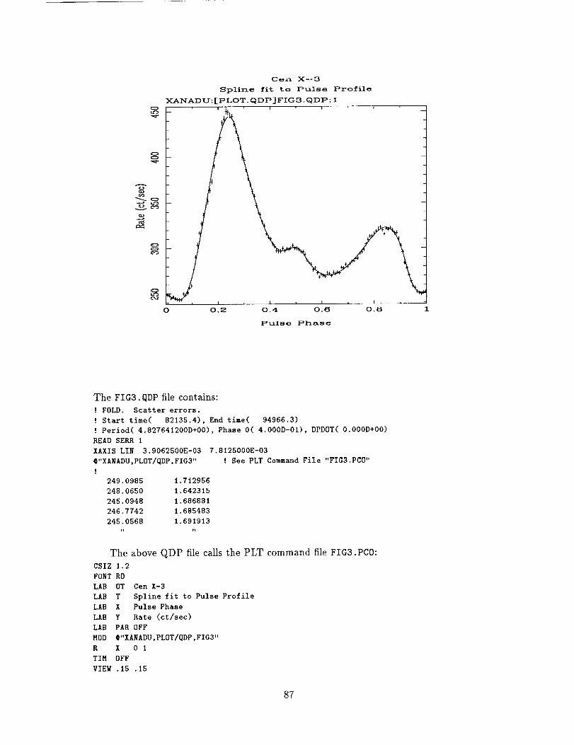
Cen X--3
Spline fit to Pulse Profile
](ANAD U: [PLOT. QDP] FIG3. QDP ; 1
0
0
0
o
v
0
0
Ok2
0.2 0[4
I ' I " I ' I '
I I I ,
0.6 06.
Pulse Phase
1
The FIG3. QDP file contains:! FOLD. Scatter errors.
! Start time( 82135.4), End time( 94966.3)
! Period(4.827641200D+00), Phase O(4.000D-01), DPDOT(0.000D+00)
READ SERR 1
XAXIS LIN 3.9062500E-03 7.8125000E-03
@"XANADU,PLOT/QDP,FIG3" ' See PLT Command File "FIG3.PCO"
!
249. 0985 1.712956
248. 0650 1.642315
245.0948 1. 686881
246. 7742 1. 685483
245.0568 1.691913
ii
The above QDP file calls the PLT command file FIG3.PCO:
CSIZ 1.2
FONT RO
LAB OT Cen X-3
LAB T Spline fit to Pulse Profile
LAB X Pulse Phase
LAB Y Rate (ct/sec)
LAB PAR OFF
MOD @"XANADU,PLOT/QDP,FIG3"
K X Ol
TIM OFF
VIEW .15 .15
87

"7
e¢-)
Jo
CROSS--SCAN PROFILES
XANADU: [PLOT. QDP]FIC#.QDP; 1
i ' ' t
° High Energy
o Low Energy
0 10 20 30 40 50
RA PIXEL
The FIG4. QDP file contains:READ SERR 1 2
@" XANADU, PLOT/QDP, FIG4"
1.00 0.50 -1.E-01 3.1
2.00 0.50 -0.4 3.1
3.00 0.50 -1.9 3.1
4.00 0.50 2.8 3.1
5.00 0.50 3.7 3.1
6.00 0.50 0.3 3.1
7.00 0.50 0.2 3.1
8,00 0.50 5.5 3.1
9.00 0.50 -4.7 3.1ii
! See PLT Command File "FIG4.PCO"
SKIP
LINE
MARK
LINE
MARK
MARK
LAB
LAB
LAB
LAB
LAB
LAB
LAB
TIME
The above QDP file calls the PLT command file FIG4.PC0:SING
ON I
17 ON 1
0N 2
21 ON 2
SIZE 1.5
1 MAR 17 JUS Lef
I POS 36 45 "High Energy"2 MAR 21JUS Lef
2 POS 36 41 "Low Energy"T CROSS-SCAN PROFILES
X RA PIXEL
Y Background Subtracted Intensity (kJy Sr\u-l)OFF
88
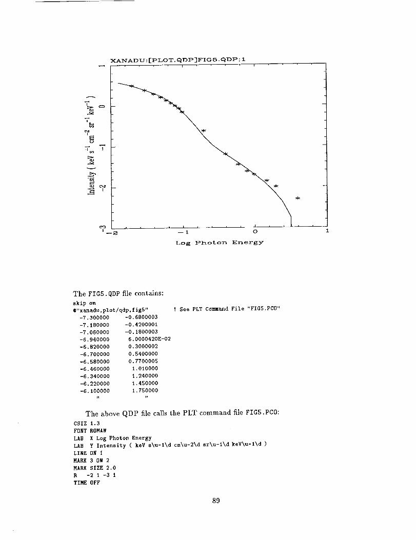
"7'T °
$--4
C.)
DO
(1)
I--2
XANADU: [PLOT.QDP]FIGS.QDP; I
I u
l n , | | i
--i O
Log Photon Energy
L
1
The FIGS. QDP file contains:
skip on
@"xanadu, plot/qdp, f ig5"
-7.300000 -0.6800003
-7.180000 -0.4200001
-7.060000 -0.1800003
-6.940000 6.0000420E-02
-6.820000 0.3000002
-6.700000 0.5400000
-6.580000 0.7700005
-6.460000 1.010000
-6.340000 1.240000
-6.220000 1.450000
-6.100000 1.750000
! See PLT Command File "FIG5.PC0"
The above QDP file calls the PLT command file FIGS.PC0:
CSIZ 1.3
FDNT ROMAN
LAB X Log Photon Energy
LAB Y Intensity ( key $\u-l\d cm\u-2\d srku-lkd keV\u-lkd )
LINE OR 1
MARK 3 ON 2
MARK SIZE 2.0
R -2 1 -3 1
TIME OFF
89

f[g6.qdp
_4
.
! I
5 10 15 20 25 30
The FIG6. QDP file contains:
COL OFF 1..999
CDN LEV -1. -.5 O• .5 1. LS 4 4 1 1 1 LW 1 2 3 4 5
XAX LIN 1 1
YAX LIN 1 1
R 1 30 1 30.i
.748 .795 .826 •842 .841 .823 •788 .734 .664 .577 .474 .358 .228-
8.700E-02 -6.300E-02 -.220 -.383 -.548 -.713 -.876 -1.035 -1.187 -1.331-
-1.464 -1.585 -1.692 -1.783 -1.859 -1.917 -1.958
.499 .574 .639 .691 .731 .755 .764 .756 .731 .689 .631 .555 .464-
.358 .239 .107 -3.400E-02 -.184 -.340 -.500 -.662 -.823 -.981 -1.135-
-1.281 -1,418 -1•545 -1•658 -1.758 -1.842
,281 .364 .442 .513 .573 .622 .658 ,681 .688 .679 .654 .613 .556-
.483 .395 .292 .177 5.000E-02 -8.600E-02 -.230 -.381 -.535 -.691 -,846-
-.999 -1.147 -1,289 -1.422 -1,544 -1.654ii
90

iii
NASA TM-4301
4. T,tle and Subt,fle
The QDP/PLT User's Guide
7 A_Jlhorlsl
Allyn F. Tennant
9 P_r'lorm,%l ()rgani/ation Name and Address
George C. Marshall Space Flight Center
Marshall Space Flight Center, AL 35812
Report Documentation Page
2. Government A'ccession No. '"'
12. Sponsoring Agency Name and Addf.ss
National Aeronautics and Space Administration
Washington, DC 20546
15. Supplementary Notes
3. Rec=p_ent's Catalog No
5. Report Date
June 1991
6 Performing Organization Code
E365
8. Pedo, mmg Organization Report No.
I0. Work Unit No.
M-662
I1. Contract or Grant No
tJ. Type of Report and Period Covered
Technical Memorandum
14 Sponsoring Agency Code
Prepared by Space Science Laboratory, Science and Engineering Directorate.
16 Abstr;,Cl
PLT is a high level plotting package. A Programmer can create a default plot
suited for the data being displayed. At run times, users can then interact with
the plot overriding any or all of these defaults. The user is also provided the
capability to flt functions to the displayed data. This ability to display,
interact with, and to fit the data make PLT a useful tool in the analysis o£ data.
The.Qulck and Dandy Plotter (QDP) program wlll read ASCII te_t files that contain
PLT commands and data. Thus, QDP provides an easy way to use the PLT software.
QPD files provide a convenient way to exchange data. The QPD/PLT software is
written in standard Fortran 77 and has been ported to VAX VMS, SUN UNIX, IBM AIX,
NeXT NextStep, and MS-DOS systems.
Requests for software should be addressed to: COSMIC, The University of Georgia,382 East Broad Street, Athens, GA 30602.
Suggestions for improvements or reports of software bugs should be addressed to
the author: Allyn Tennant, ES65, NASA, MSFC, Huntsville, AL 358[2, U.S.A.,
Telephone: 205-544-3424; Fax: 205-544-7754. SPAN:SSL::TENNANT or 7207::
TENNANT; Internet: tennant%[email protected]
17. Key Words (Suggested by Author(s)) t8. Distribution Statement
Data Analysis
Graphics Unc]asslfied-Unlimlted
Subject Category: 61
_9, Security Classif. (ol lhis repot)
Unclassified
_. Secur,tV Classif. (of this pagel 21. No. of paqes
Unclassified 93
22. Price
A05
NASA FORM 1_ OCT
For sale by the National Technical Information Service, Springfield, VA 2216[-2171
NASA-LangI_, 1_1

_¢


