UNCLASSIFIED

AD NUMBER

AD-530 009

CLASSIFICATION CHANGES

TO UNCLASSIFIED

S................................................................................................................................................

FROM CONFIDENTIAL

AUTHORITY

OCA; Dec 31, 1980 IAW Document Markings

THIS PAGE IS UNCLASSIFIED

UNCLASSIFIED

AD NUMBER

AD-530 009

NEW LIMITATION CHANGE

TODISTRIBUTION STATEMENT: A

Approved for public release; Distribution Unlimited.

LIMITATION CODE: 1

FROM DISTRIBUTION STATEMENT: B

LIMITATION CODE: 3

AUTHORITY

RADC Ltr; Nov 8, 1982

THIS PAGE IS UNCLASSIFIED

U LB

ACCL'3TIC SOCU2E LCCATTIDzI U'TING LON'IG SiISE

clot Dr. Jaime., G. Con.;tantirne1/Lt Mark D. Dickinson

RATIONAL SECU'RITY I N7V0 PA-.TI1ONUnauthorized disclosure~ subject to crimina~l sanctiors

-. - Distribution limited to. U.S. Gov't agencies only;foreign info M larch 1974.Other requepts for this d:)cuient must be referredto RADC (DCTI), GAFB, NY 13441. .

JE TIT GSý,?!tY.4 PCLAES'7CITCN Z S

FC77, OF !-l1TV 47,F QDTR 31f,32.~T~~7DJ:~Y~7:~AiJAT TVýrO

YT-1 I!'777,A' JED

Rome Air Development Center- ~Air Force Systems Commanid

(D Griffiss Air Force Base, New York,U cc:

J4

Do not return this copy. Whnnot needed, destroyin, accordance with pertinent. security Mglatioufl.

NVRADC-TR-73-37OACOUSTIC SOURCE LOCATION USING LONG BASE LINL TECHNIQUES (U)

0~arch 1974

0 Confidential Report

(%2 UNCLASSIFIED

ERRATA

June 1974

Please make the following insertion and correction to subject report:

1. Insert on the front cover:

"Classified by 692B SCGSubject to GDS of EO 11652Automatically dcwngraded attwo year intervalsDeclassified on 31 Dec 1980"

2. In Block 15a of DD 1473, delete "GDS - Decl. 31 Dec 79" andinsert "GDS - Decl. 31 Dec 1980"

Rome Air Development CenterAir Force Systems Command

Griffiss Air Force Base, New York

ji

UNCLASSIFIEDSECURITY CLASSIFICATION OF THIS PAGE (I?*,Does Snm -d)

READ INSTRUCTIONSREPORT DOCUMENTATION PAGE BEFORE COMPLETING FORM

V. REPORT NUMBER 2. GOVT ACCESSION NO. J. RECIPIENT'S CATALOG NUMBER

RADC-TR-73-3704. TITLE (and S,~bftf1a) S. TYPE OF REPORT & PERIOD COVERED

ACOUSTIC SOURCE LOCATION USING LONG BASE In-House (Mar..- Sep. 72)

LINE ECHNIUES5. PERFORMING ORG. REPORT NUMBERRADC-TR-73-370

7. AUTHOR(.) S. CONTRACT OR GRANT NUMBER(.)Dr. James G. ConstantinelILt Mark D. Dickinson N/A

9. PERFORMING ORGANIZATION NAME AND ADDRESS 10. PROGRAM ELEMENT. PROJECT, TASK

Rome Air Development Center (OCDE) AE OKUI UBR

Griffiss Air Force Base, New York 13441 Job Order No. 692B0205

v 1. CONTROLLING OFFICE NAME AND ADDRESS 12. REPORT DATE

Rome Air Development Center (OCDE) Mrh17

Griffiss Air Force Base, New York 13441 13. NUMBER OF PAGES48

14. MONITORING AGENCY NAME & ADDRESSQIl dlffavant from Controtttng OffIco) IS. SECURITY CLASS. (of this .aport)

Confidential

IS*. DECLASSIFICATION/ DOWNGRADING

_____________________________________GDS tb'eY.3Ii Dec. 0IS. DISTRIBUTION STATEMENT (of this R.,orfO

Distribution limited to US Gov't agencies only; foreign info March 1974.Other requests for this document must be referred to RADC (OCDE), GAFB, NY 13441.

17. DISTRIBUTION STATEME14T (of ICho abe tract ontorad I, Block 20, I diffferant froaI Report)

Svae

IS. SUPPLEMENTARY NOTES

None

:19. KEY WORDS (CoIfinue on reotsra side It nac..ar~ and ldant.'fy by block sman~ber)

Cross-CorrelationAuto-CorrelationAcoustic Detection

I' Acoustic SignaturesTracking (Position)

C ~20. ABSTIRACT (Coottinuo on mveras aid., ff naeoasin and identify' by block ntImmir)

UNCLASSIFIED ABSTRACTAstudy is made of acoustic base line methods for detecting and locating srae sound sources such as

trucks. The experimental system used is composed of widely separated omnidirectional receivers and a signalprocessor which operates on the receiver outputs. The long base lines and the highly periodic nature of theacoustic signals generated by engines of any type lead to severe ambiguity In acoustic source location.Mathematical derivations and experimental analysis have led to signal processing techniques which reduce the

periodic components of the source signals and preserve the random Signal components for use in time-of-arrival

DD ,2IS1473 EDITION Ol" I NOV 69 IS OBSOLETE UCASFE

IIIICUPRITVf CLASSIFICATION OF THIS PAGE (Who"t Date Entorad

UNCLASSIFIED

SECURITY CLASSIFICATION OF TH.IS PAAG(WlSh D0..a. , '.-d)

20. ABSTRACT (continued)

measurements. Subsequent tource location is highly successful. In the present analysis: (a) a source whose

sound-pressure level (SPL) is about 100 dB re 0.0002 microbar and whose signal contains strong peribdic

components was detected and Iocated using base lines of about 1000 meters; (b) accuracies in locating the

sound source of several meters were achieved under calm weather conditions; and (c) identification of the

sound soi~rces was successfully performed based on spectral signatures.

S...... . . ........ .. ..... .... ... ... .. ..... . . ... . . ..

sI-

Ti ,curr'r WFi PAOK(I~ a asBfw

__.....__NCA_ IFIED

SUMMARY

A study is made of acoustic base line methods for detecting and lcating surface sound sources such as trucks.* The experimental system used is composed of widely separated omnidirectional receivers and a signal processor

which operates on the receiver outputs. The long base lines and the highly pediodic nature of the acoustic signalsgenerated by engines of any type lead to severe ambiguity in acoustic source location. Mathematical derivationsand experimental analysis have led to signal processing techniques which reduce the periodic components of thesource signals and preserve the random signal components for use in time-of-arrival measurements. Subsequentsource location is highly successful. In the present analysis: (a) a source whose sound-pressure level (SPL) isabout 100 dB re 0.0002 microbar and whose signal contains strong periodic components was detected and locatedusing base lines of about 1000 meters; (b) accuracies in locating the sound source of several meters were achievedunder calm weather conditions; and (c) identification of the sound sources was successfully performed based onspectral signatures.

/3

/

/S~/

iI

H

• I 1" -- -,?

PREFACE

The study described in this report was accomplished in-house In the Surveillance Equipment DevelopmentBranch of Rome Air Development Center, under Job Order Number 692130205.

This report contains classified information extracted from the two classifit.i documents asterisked in theReferences.

The authors wish to express their gratitude to Lt Col R.C. Salisberry and Mr. E.F. Krzyslak of RADC for theirsuggestions in analyzing the 'echnical data and for their support during this effort. They alsc wish to thank CaptD. Hammond and Mr. M. Cione, both formerly of RADC, for their contributions in signal processing and forwritinig many of the computer programs.

This technical report has been reviewed and is approved.

APPROVED: ( - . 4 j ,.JOSEFH M. EANNARINOChief, Surveillance Equipment Development BranchSurveillance & Control Division

APPROVED: I ... . . ._

WILLIAM T. POPEAssistant ChiefSurveillance & Control Division FO. THEOMMANDER

FOR THE COMMANDER:6

CARLO P. CROCETTIChief, Plans Office

2

•-j-~JIa.u~s .. ,......y;..> - - . .

TABLE OF CONTEN TS

PAGE

1. INTRODUCTION.......................................................... 7

It. THEORY................................................................ 8A. Correlation Analysis.................................................... 8B. Time-of-Arrival Techniques................................................ 9C. Signal Prewhitening..................................................... 10D. Spectral Analysis......................................................I i

Ill. EXPERIMENTAL APPARATUS AND EXPERIMENTAL ARRAN(JtEMENT .................. 12A. Target-Sensor Configuration............................................... 12B. Sensor System Description (Phase Ill Commikes)................................. 12C. RADC Acoustic System................................................. 16

1. Sound System...................................................... 16a. Broad Band Noise................................................. 16b. Swept Tones..................................................... 16c. Moving Target (Truck) ................ I.............................. 17d. Interfering Targets--------------------------------------------------17

2. Microphones--------------------------------------------------------173. Micrometeorologic~al Instrumentation---------------------------------------17

4.Recording Equipment................................................. 17

IV. ANALYSIS AND RESULTS.................................................. 18A. Spectrum Analysis..................................................... 18

2. Source Spectrum.................................................... 18

B. Correlation Analysis.................................................... 211. Results and Interpretation.............................................. 23

V. SUMMARY AND CONCLUSIONS.............................................. 40References.............................................. I................ 43

APPENDIX.................................................................. A-I

FIGURES

FIGURE NO. TITLE PAGE

I. Location of a Sound Source by Triangulation ................................ 9

2. Source and Sensor Locations at Auxiliary Field Nc. 6 Eglin AFB FL .............. .13

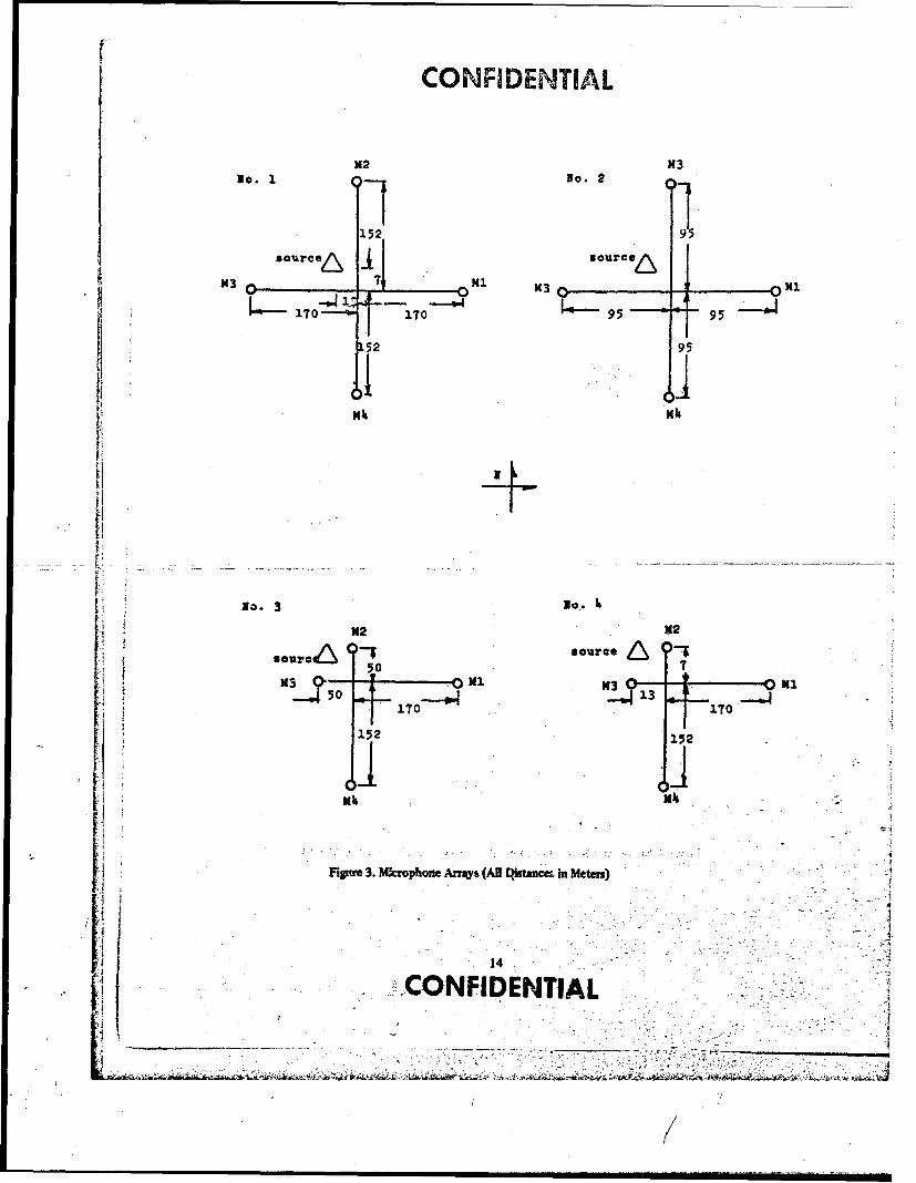
3. Microphone Arrays (All Distances in Meters) ............................... 14

4. Phase III Commike Modification for PAVE ONYX Mission ..................... 15

5. S-Band Data Link for Phase PI Commikes ................................. 16

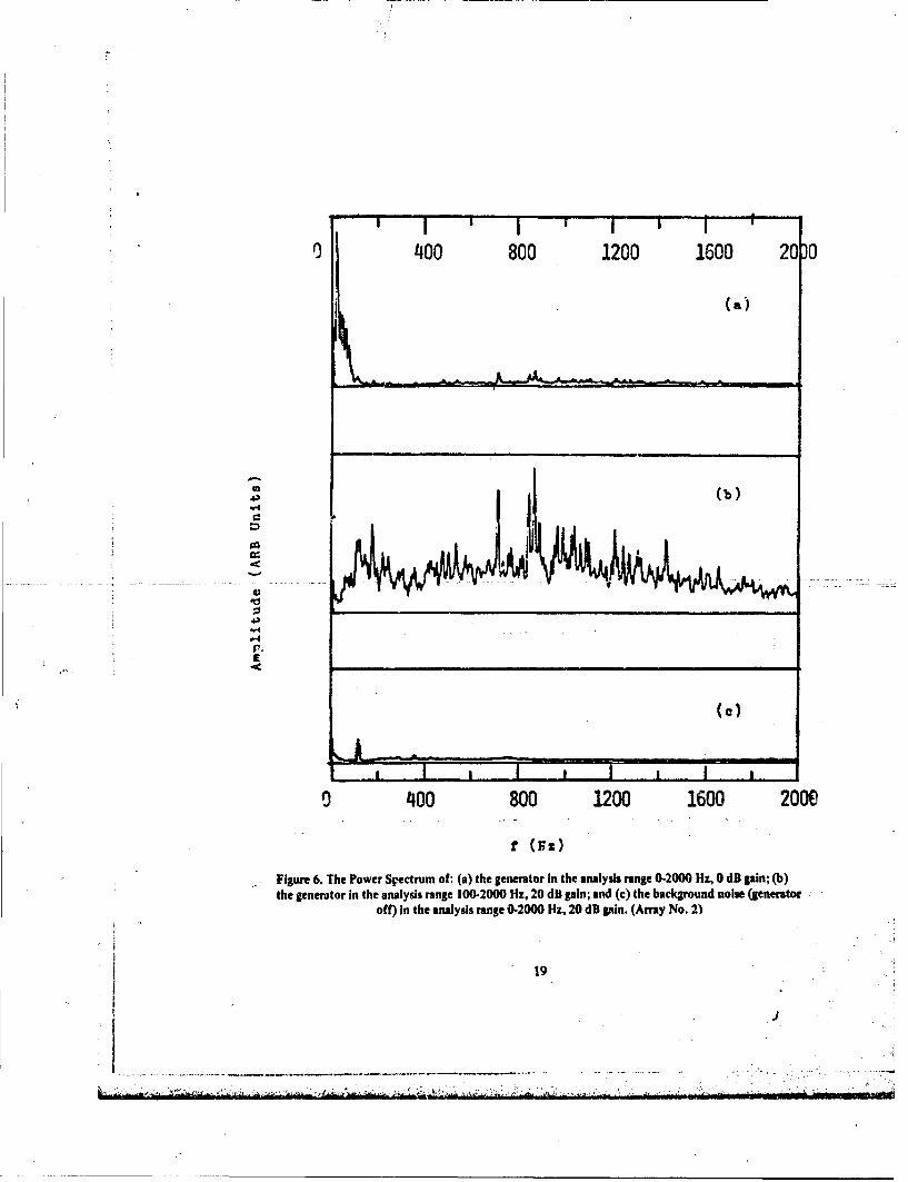
6. The Power Spectrum of: (a) the generator in the analysis range 0-2000 Hz, 0 dB gain;(b) the generator in the analysis range 100-2000 Hz, 20 dB gain; and (c) the backgroundnoise (generator off) in the analysis range 0.2000 Hz, 20 dB gain. (Array No. 2) ...... 19

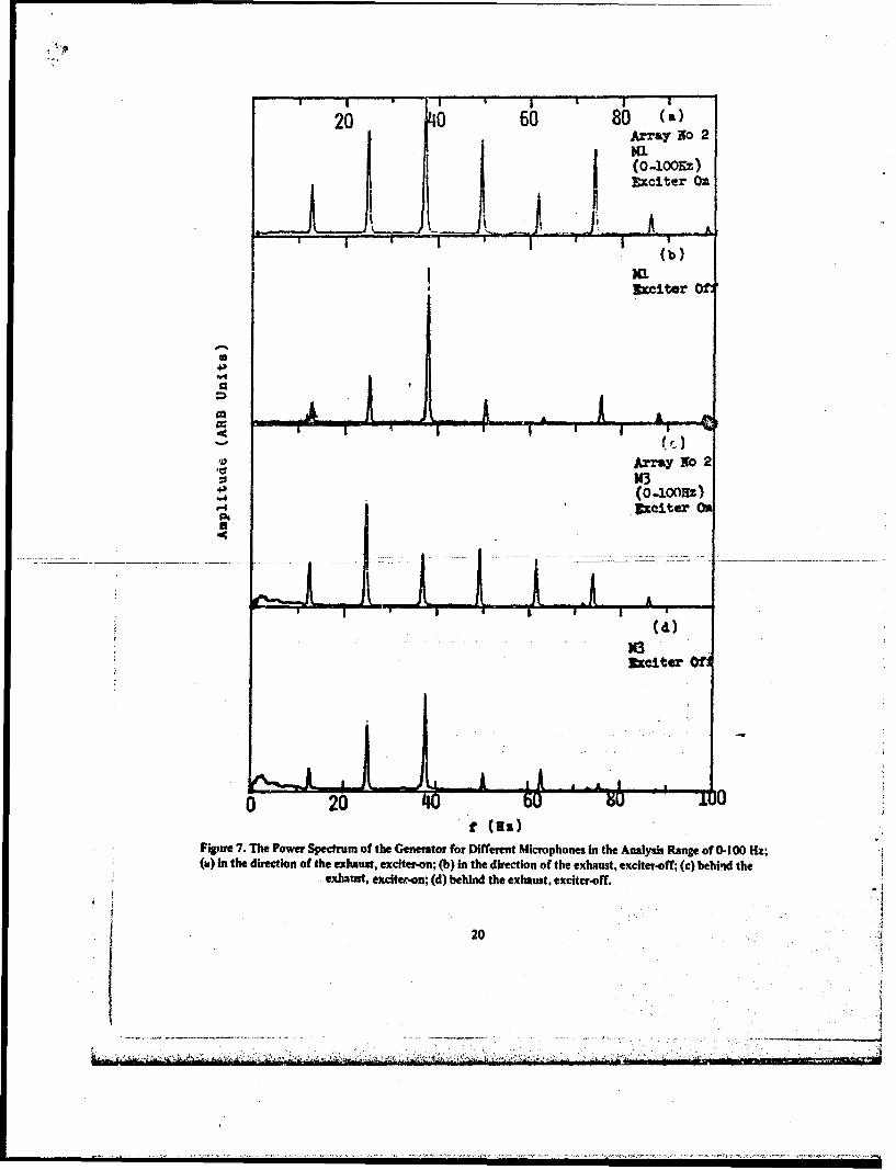
7. The Power Spectrum of the Generator for Different Microphones in the Analysis Rangeof 0-100 Hz; (a) in the direction of the exhaust, exciter-on; (b) in the direction of theexhaust, exciter-off; (c) behind the exhaust, exciter-on; (d) behind the exhaust, exciter-off ............................................................. 20

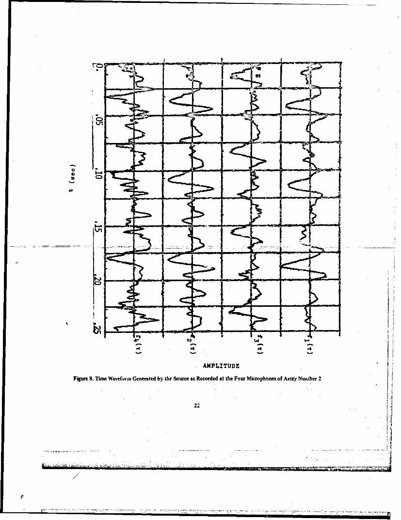
8. Time Waveform Generated iy the Source as Recorded at the Four Microphones of ArrayNumber 2 ......................................................... 22

9. Time Waveform Generated by the Source: (a) exciter-on; (b) exciter-off ............ 23

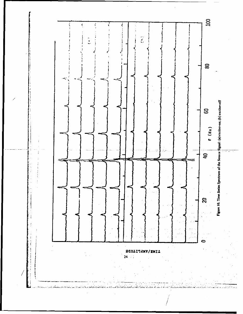
10. Time Series Spectrum of the Source Signal: (a) exciter-on; (b) exciter-off .......... 24

11. Cross-correlation Function of MI 's M2: (a) source Aignal; (b) 40-80 Hz band-limitedwhite noise; ard (c) 40-150 Hz swept tones .-.............................. 25

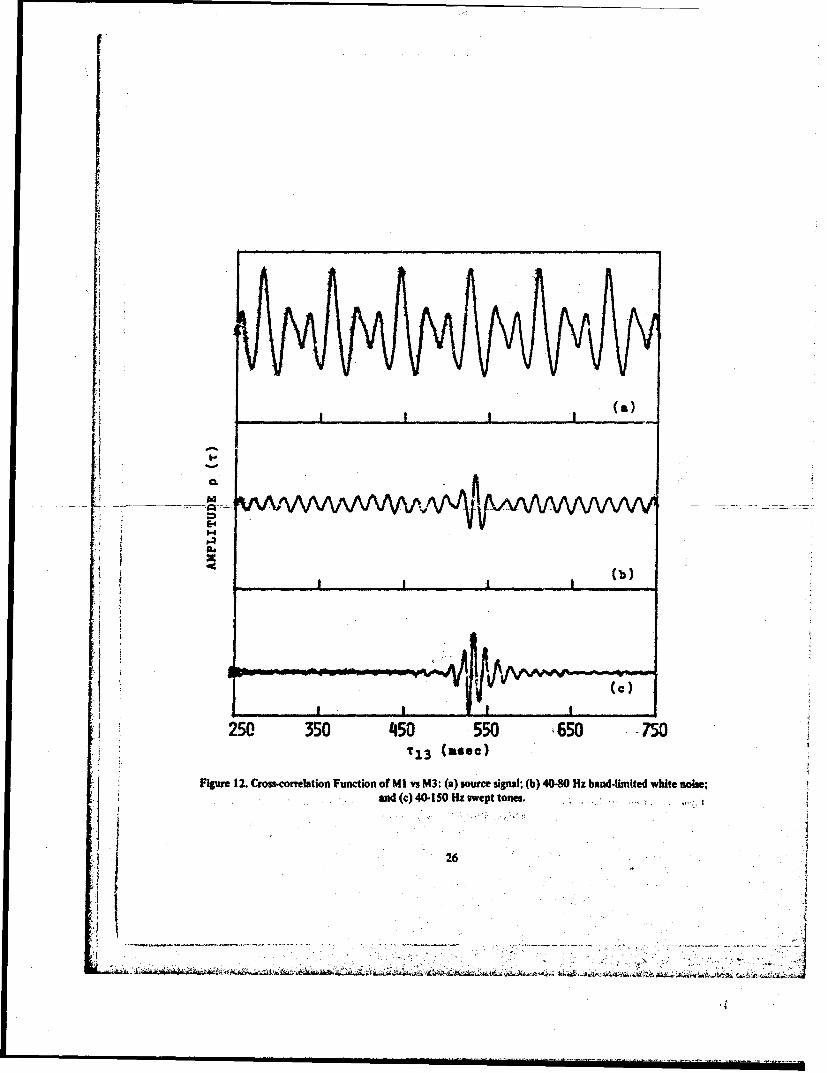
12. Cross-correlation Function of Ml vs M3: (a) source signal; (b) 40-80 Hz band-limitedwhite noise; and (c) 40.150 Hz swept tones .............................. 26

13. Cross-correlation Function of MI vs M4: (a) 40-80 Hz band-limited white noise; (b)40-150 Hz swept tones; and (c) source signals .............................. 27

14. Cross-correlation Function of M2 vs M3: (a) source signals; (b) 40-80 Hz band-limitedwhite noise; and (c) 40-150 Hz swept tones .............................. 28

IS. Croass-correlation Function of M2 vs M4: (a) source signals; (b) 40-80 Hz band-limitednoise; and (c) 40.150 Hz swept tones .................................. 29

16. Cross-correlation Function of M3 vs M4: (a) source signals; (b) 40-80 Hz band-limitednoise; and (c) 40- t50 Hz swept toncs .................................. 30

4

/

FIGURES (Cont'd.)

FIGURE NO. TITLE PAGE

17. Auto-correlation of 100-1000 Hz band-limited: (a) source signal; (b) background noise . 32

18. Cross-correlation Function of M3 vs M4 (Array No. 4) over the Analysis Range 0-500msec. Band-Limited Source Signals: (a) 100-1000 Hz; (b) 150-1000 Hz; (c) 50-1000 Hz;and (u) band-limited white noise 160-320 Hz ............................... 33

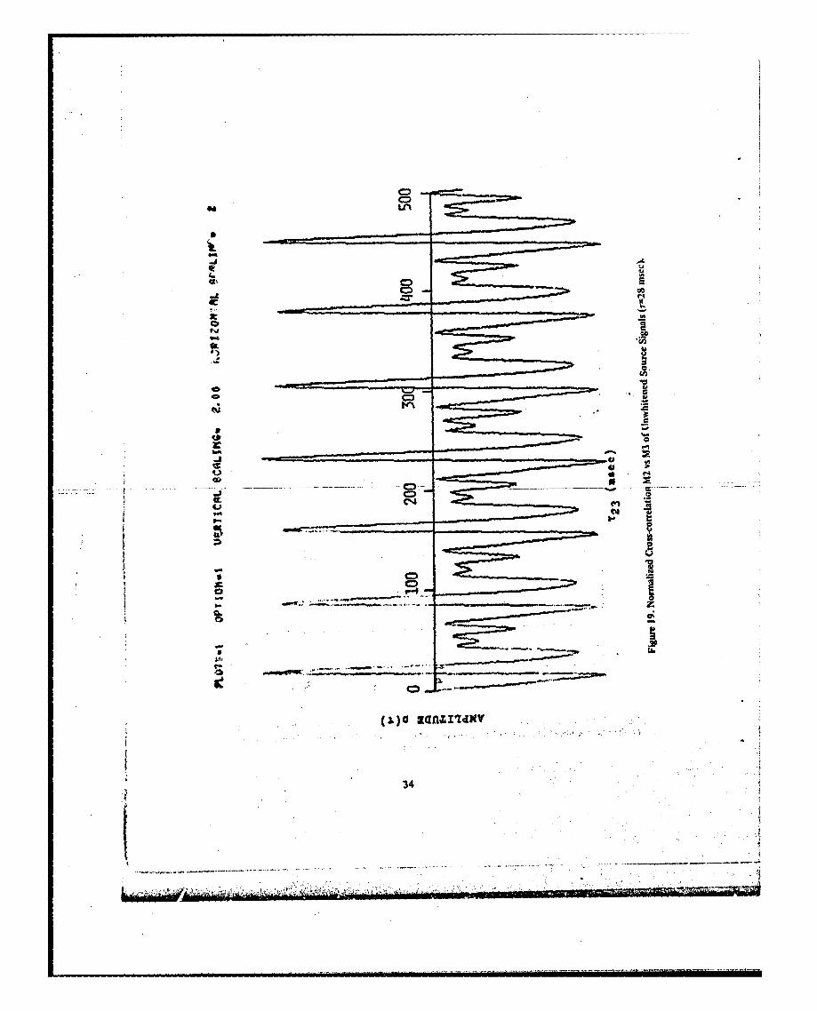
19. Normalized Cross-correlation M2 vs M3 of Unwhitened Source Signals (r=28 msec) .... 34

20. Normalized Cross-correlation M2 vs M3 of Log-Whitened Source Signals ............ 35

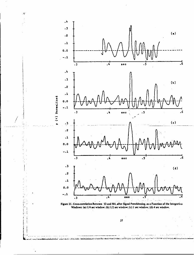
21. Cross-correlation Between M3 and M4, after Signal Prewhitening, as a Function of theIntegration Windows: (a) 1/4 sec window; (b) 1/2 a.c window; (c) I sec window; (d) 4sec window . .................................................... 37

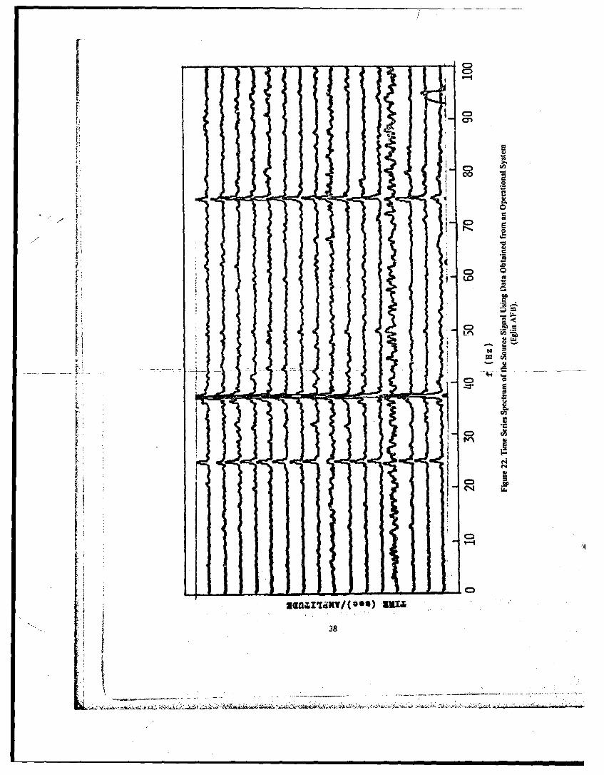
22. Time Series Spectrum of the Source Signal Using Data Obtained from an OperationalSystem (Eglin AFB) .............................................. 38

23. Cross-correlation Function of Source Signals after Prewhitening Using the IGLOOW HITE System .................................................. 39

24. Block Diagram of Digital Prewhitening Technique as Applied to the Cross-Spectral PowerDensity ........................................................ A-3

.. --- --- TABLE _ __-_ _

TABLE NO. PAGE

I Correjation Analysis (Array No. 4) .................................... 31

77I

1 !K-<

1. (U) Introduction

The purpose of this work was to assess experimentally the feasibility of locating power generators by time-correlating their acoustic energy relayed by three or more spatially-separated acoustic sensors. Correlation tech-niques are very commonly used in the process of localizing noise sourcs(1-11) and many of the factors affectingsound-ianging are well understood(1 2).

The specific problem addressed in this work was eliminating the spurious maxima from the correlationfunction of the generator signal. These spurious maxima result from the dominant periodic compone.ts existing inthe generator's acoustic signal. Depending on the nature of the sensor configuration and the particular generatortested ten or more maxima of equal amplitude may appear in the correlation functlon. This makes it difficult tocorrectly identify the true correlation maximum.

This report discusses a successful technique to eliminate the effect of periodic components from the correlationfunction and defines relatively simple methods of correctly identifying these types of targets. Chapters 1I, 1ll, IV,and V, respectively, di-'zss the theory behind this experiment, the experimental apparatus and mcrophone con-figuration, the experimental analysis and results, and summarize the findings..

N o

?7

\* ---.-----.-..--------------. ---.-..--- ------..----- -.. .--

II. (U) Theory

The location of sound sources is done by using time-of-arrival techniques. To establish the coordinatesof the acoustic source by this method the following must be known: (a) a minimum of two independent deliý times(time differences between the same event received at several microphone lecations); and (b) the correspondingmicrophone separating distances (base lines). In practice, the microphone array configuration is known and the onlyparameters to be measured are the delay times between the elements of zt least a threc-rmicrophone array. If theacoustic source is of impulsive nature the time difference between signals received at several microphone locationsis easily defined. This, however, is not so in the case of continuous sinials. In the latter case cross-correlation tech-niques can achieve results analogous to those obtained for the pulse case.

A. Correlation Analysis

The cross-correlation of two waveforms is a measure of their similarity as a function of the time shift betweenthem. Mathematically this can be achieved by computing the cross-correlation function. That is, the two signals aremultiplied and summed over a specified time window T. This is done for different values of time 7. For the value ofr at which the two signals match, a maximum value of the correlation function is obtained. This value of r is equalto the delay time of one signal relative to the other. The mathematical expression for the discrete cross-correlationfunction is:

N+m'IRij ( N,k) = - Xi(n)X (n-k) (1)

n=m

Here, Xi(n) ;s the signal on channel i at the nth sample instant, Xj(n-k) is the signal on ckannelj at the (n-k)thsample instant, k is the delay between channels in samples, N is the correlation window in samples, and m is thesample instant for start of the correlation window.

In the case of discrete plotting of a series of measurements in the form of pairs of observation points Xi(n;and -(n), a normalized measure of correlation lying between -1 and +1 is often desirable. The di3ital fcrm of -1-

. normalized correlation is: ........ ... . [" .. ...1"flS........ .. ..... . IF ~ ~N+m - r N+m -- -- l tz . . .. .... .. . . .Pi r~):Rij(m,k) • X2 (n)]•X~

The normalized correlation function was suggested as a method to reduce spurious correlation maxim%.rationale behind it is as follows: Write Eq (1) as,

Rij(m~k) oi(m) oj(m-k) P!(ij-(,k) " -

where, r N+m 1/2

oi(m)X 2 (n) (4)

If there is a large change in energy in the signal from one correlation record to the next, then it is possiblethat,

Ri3 (ml,kl) > Rij(m2, k2) (5)

8

w a "I

while,Pij(m I. k I)< Pij (m2, k,) (6)

simply because

ai (nI ) oj (mj -"kl) »> a1 (in2 ) o1 (m 2 "k2 ) (7)

If the signal is quasi-stationary in the sense that its spectral shape does not change with time, then Pij will beindependent of the recorl time m. Hence it will be a more consistent estimator of the true correlation maxima thanRij if the signal energy. above, is non-stationary.

For an example, consider the application of correlation techniques to an acoustic receiving system consisting'I of a three-element aaray. The coordinates of the array relative to a known origin, in this case a control processing

center, will be known.

B. Time of Arrival Techniques

In Figure 1 the field deployment of such an array is illustrated. It ha. been mentioned above that the signalfrom the source, whose position relative to the array is S (X,Y), arrives at different times at M 1, M2, and M3. Thedifference in time-of-arrival (delay time r) can be detennined using cross-correlation techniques. Using the delaytime to locate the source of disturbance one must find a relationship between r and the geometry of the system.To simplify Lhe calculations we have assured a planar geometry (i.e., Z=Z1 =Z2 Z3 ). If this is not the case anarray of at least four sensors is required to locate the sound source.

Y__ - - 4M2(x 2, Y2 )

Vt 2iVt

" s(zX Y)

Ri \Vt3R2 /

R • 3 (X3 , Y3)

- R3

0 x

'- Figure 1. Location of a Sound Source by Triangulation

9

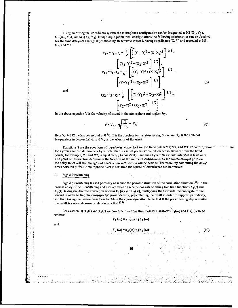
Using an orthogonal coordinate system the microphone configuration can be designated as M I(X1 , Y1),M2(X 2, Y2), and M3(X 3 , Y3)" Using simple geometrical configurations the following relationships can be obtainedfor the time delays of the signal produced by an acoustic source S having coordinates (X, Y) and recorded at Ml,?A2, and M3:

I2 = t t 2 ("I )2÷(XXI)2 1/2

(ya. Y)2 + (X 2.yX)2+ 1/2

: ~In the above equation V is the velocity of sound in thle atmosphere and is given by:

; V=Vo. ~f + vw (9)

__ Here Vo 332 meters per second at 0 °C, T is the absolute temperature id degrees kelvin, TO is the ambient

Stemperature in degrees kelvin and Vw,, is the velocity of the wind.

"__ ...- ..... Equations S-are-the equations of hyperbolas whose foci are the fixed pointsMI.Mt2,-and M3.Therefore,- :• -: ---- =•S~for a given i we can determine a hyperbola, that is a set of points whose difference in distance from the fixed

: points, for example, M1 and M2, is equal to T1 2 (a constant). Two such hyperbolas should intersect at least once.The point of intersection determines the location of the source of disturbance. As the source changes position

the delay times will also change and hence a new intersection will be defined. Therefore, by computing the delay

times between different microphone pairs in real tine the source of disturbance can be tracked.

Sf ~C. Signal Prewhitening

Signal prewhitening is used primarily to reduce the periodic structure of the correlation functiont i 0 ) In the

Si present analysis the prewhitening and cross-ccrrelation scheme consists of taking two time functions Xl(t) andX2 (t), taking the discrete Fouaier transforms F1 (w) and F2 (w), multiplying the first with the cofjugate of thesecond in order to find the cross-spectral power density, prewhitening the result in order to suppress periodicity,

and then taking the inverse transform to obtain the crosscorrelation. Note that if the prewhiteaing step is omittedthe result is a normal cross-correlation function.(13 u

tmFor example, if Xf(t) and X2 (t) are two time functions their Fourier transforms Fb(e ) and F.(w) can be

C written:

i ~~FI (o) =al (o) + jbI (wa)

=• andX F 2 (r ) F a 2 (w) +a Jb 2 (mp) (10)

st

n I F2 10w)j2W)(0

•1;X111

CONFiDENTiAL

Then the cross-spectral power density is:

SI, 2(w) = Fl(j) F'2(W) = [aI (o) a2 (wo) +b 1(c)b2(wo)

+ j [a2(co) b I () - b2(cM)al (M)J"

Any prewhitening scheme in the frequency domain can be considered to be a multi, lication of S1 2(w) by a functionK2 (w).(10) In general, there are no restrictions placed on K2 (w). However, in order to preserve phase inforrmiation,K2(co) is required to be positive real. After performing the multiplication we have,

T 1,2 () = S1 ,2 )K2 (o) (11)

where,

K2 ((w) Qn(a 2 + 32) (12)

2[a 2+o2J 1/2here,

a i11()a 2 (w)+bI(w)b 2 (w)and

= a2() bI ()-b2()aI (C) (13)

At this point take the inverse transform of T 1,2(o). Using the convolution theorem the inverse transform of T 1,2(w)equals the inverse transform of S 1,2(w) convolved with the inverse transform of K2(co). Then since the inversetransform of S1,2(w) is the cross-correlation R 1,2 (r) of Xl(t) and X2(t), the result is the corss-correlation ofXl(t) and X2 (t) convolved with a function k(r), where k(r) is the inverse transform of K2 (w).

! .D. Spectral Analysis

.. . . Spectral analysis is based upon computation of the Fourier integral:

S(fW)= X(t)exp(-2ift)dt (14)

In order to understand how computation of the Fourier integral helps to make meaningful measurements, considerthe Fourier transform written in its sine-cosine form:

SX (0I X(t) (cos 21rft - j sin 21rft) dt (15)

This equation states that the transform averages a time function input X(t) with a set of sines-cosines to determinethe content of X(t) at some frequency f. Thus the transform resolves the time function into a set of components atvarious frequencies much as a set of analog filters would. However, it not only yields the amplitude of each frequency,but also resolves the in-phase (real, cosine) component and the quadrature (imaginary, sine) component, therebygiving magnitude and phase information which is difficult to obtain in any other way.

CONFIDENTIAL(This page is Unclassified)'

CONF!DENTIAL

11I. (U) Experimental Apparatus and Experimental Arrangement (U)

A. (C)_Target :-Sensor Configuration (U)

(C) The target, 50 Hz, 75 KVA generator motor set, was tested in a semi-jungle environment area on Auxiliary

Field No. 6 at Eglin AFB, Florida. The test was conducted in order to establish criteria for locating and identifyinggenerator type targets. Figure 2 depicts the relationship between the sound source and the sensors. The detectionsystem consisted of modified Phase II commikes (MCOM), hand-emplaced commikes (HEC), and an RADC acousticsystem. The Phase III commikes were connected to a central recording station via an RF link, while the RADC

microphones were hard-wired into a recording system.

(C) The MCOM and HEC were placed at points designated by stake markers on the four legs (north, south, east,

and west) from the source. The stakes were in 100-meter increments up to 1 kilometer and from there in 500-meterincrements up to 2 kilometers. The source as indicated in Figure 2 was positioned off-center. The location wasapproximately 20 meters from center on the north leg and approximately 8 meters from center on the west leg. Itshould be noted that the exhaust was directed parallel to the east leg.

(C) The two MCOMS and one HEC were collocated on each of the four legs. Two MCOMS allowed for backupdata in case a MCOM failed during a test. The HEC gave continuous audio data for evaluation of the audio signalat any time during the operation of the MCOMS.

L (C) The RADC acoustic microphones were positioned at various points along the four legs of the test array.Figure 3 depicts the four different arrays used by RADC and the positions of the microphones relative to the source.

B.(C) Sensor System Description (Phase III Commikes) (U)

(C) The HEC transmitted continuous audio while the MCOM transmitted type I messages upon recognition of the____ isource. The MCOM was commanded to the audio mode at various times throughout the test. The MCOM consist- of

a Phase III commike modified byIA -(Nav rDevelopmeit Center). The commike was modified to consistof detc,. on circuitry which was included in the audio module,( 14) as shown in Figure 4.

(C) The detection circuitry consisted of a phase lock loop which sweeps from 72 to 78 Hz nominal. A signalwithin this frequency range must be present at least 10 seconds (enable timer) before the unit will begin to processthe signal. After the 10-second period, the signal must be present for 7 minutes more (verification timer), with nodropouts exceeding 10 seconds. At the end of 7 minutes a type I message is transmitted signifying the presences ofthe "source." If the signal should dropout for more than 10 seconds the entire process starts over with the enabletimer. At any time during the processing of the signal the MCOM can be commanded into the audio mode.

(C) There is a certain finite amount of time during which any MCOM can transmit audio after being commandedinto the audio mode. The amount of continuous audio time after a command to the audio mode is 20 secondsnominal. Since the unit's battery life is limited mainly by the number of times it transmits audio, the audio commandis used infrequently... . .

(C) The operating characteristics of the MCOM are the same as the Phase III commike but will be restated herefor clarity. The frequency response of the MCOM is from 50 to 2 KHz with output distortion les3 than 10% for theaudio mode. The output noise level is 24 millivolts nns maximum while the instantaneous dynamic range is 32 db.

12

CONFIDENTIAL:1

CONFIDENTIAL

2000NOTE: Exhaust from source 0

parallel to east leigof sensor trail. Stakenumbering In meters.

1500 torth

II 1000

roo

source

2000 1500 1000 500 500 1000 1500 2000

S• Stake Marker

500

1000

1500

1 2000

Figure 2. Source and Sensor Locations at Auxiliary Field No. 6 EgIn AFB FL

13

CONFIDENTIAL

CONFIDENTIAL

M2 MNo. 1 11 No. 2

152 5

X3rc 4Q 0- Is i M ourc* -

No. 3 so

N2 V2

~~ - source *

*31

Fipire 3. Microphone Arrays (ADI [lstances in Meter)

-14

CONFI DEI�TIAL

C

C).4-,C

�1� ___________

C 4-'4-,

�- .-

1.. Coo'-3

z0

'I' I I- - I to C I C

4-' I -

__ I-�

I I

I g�-� I �I0

.1 �0*.-* I

*f .- I..I -�,c�cj elI --I- I I

'I I7.

03

CC

CS.-U

15

CONFIDENTIAL

COWiI DENTTIAL

(C) The information transmitted by the MCOM is received, digitized, and transmitted (S-band) by an airbornesegment data link to a receiving and analy-is center. The digitizing rate is approximately 4 KHz. The digital"information is then transmitted using an S-band transmission. The link is depicted in Figure 5. The audio digitaldata is then transformed back to analog data (D/A) at the receiving and analysis center.

/

Vl:'F idI ,ceiver 7adig0 Fi.e SBavern•d iplexerLnkfr Digiplexer IlCmftk-• Fi IInterfacee

C.()RDCAosicSseUnitm

S-band Antenna

Uirectional Filter Arnl•pl i -Coupler - fier

Figure S. S-Band Data Link for Phase III Cormmies

C. (U) RADC Acoustic System

"Tne RADC experimental apparatus consisted of the sound system, microphones, the micrometeorologicalinstrumentation, ard the recording aquipment.

1. Sound System - The sound system was a 100-watt system consisting of two loudspeakers and an audiotape recorder. The speakers were Lansing Models LE 154 which have a relatively flat response in the frequencyrange 40-6000 Hz. The audio portable recorder was a Tandberg Model I 1 with frequency response 40-20,000 Hz.In addition to the generator target the following sound sources were used in this experiment:

a. Broad Band Noise - Filtered noise in octave bands were used as a noise source. The bands are 40.80

Hz, 80-160, 160-320,320-640,640-1280 Hz. The duraticn of these signals is 15 seconds each. These signals wereused to determine te ability to cross-correlate on pure noise and to compare these results with cross-correlationfunctions obtained from the "source truck" signals. In addition to noise-like signals, truck signatures contain strongspectral lines. . .

b. Swept Tones - These are swept tones and pure tones covering the frequency range between 50-150 Sdz.The structure of these signals is as follows: (1) 50 Hz for 15 seconds; (2) 50-150 Hz range swept in 15 seconds; (3)150-50 P.z swept in 15 seconds; (4) 50 Hz pure tones for 15 seconds. These signals were included in order to makedirect comparison with'the source signals which appear to sweep the same frequency range. Also, it was of interestin itself to test cross-correlation on these types of signals.

16

CONFIDENTIAL

A.I

/

c. Moving Target (Truck) - The signatures from a moving truck along a prescribed path have beenrecorded. These signatures were used as an interfering target.

d. Interfering Targets

(1) In this case three trucks were used at the same time. The trucks were separated by 100m.

(2) Prop and jet aircraft were used as interfering targets in various configurations. The masking experi-ments are designed to determine the effectiveness of cross-currelation techniques to locate and follow targets ofinterest as a function of base line in the presence of interference phenomena.

2. Microphones - In answering the question concerning the applicability of cross-correlation techniques fora stationary periodic target, four arrays of microphones were used. These are depicted in Figure 3. An array coiL-sisted of four omnidirectional microphones. The microphones are GR-P1560-953 l's and have a frequency responsewhich is flat in the range between 2 and 6000 Hz.

3. Micrometeorological Instrumentation - A meteorological system manufactured by Meteorology Research,Inc. (MRI) was used in this experiment. The instrumentation was mounted on a 6-foot tower. The system is capableof giving the temperature, wind speed, and wind direction. Using these data, information about temperature stabilityand the turbulence in the area can be obtained.

4. Recording Equipment - The signals from the microphones are hardwired to a central recording system.The lines are driven by a set of amplifiers which are gain switchable. The total dynamic range of the system is 90 dband the gain can be switched between 27 db and 97 db. The steps are 10 db each. The bandwidth of the system is2 to 2000 Hz. The output of the amplifiers was fed into a 14-channel analog tape recorder. The recorder was aHoneywell 5600 magnetic tape recorder. Out of the 14 channel- in the FM record mode four were used for themicrophones and three were used for the meteorological channels. The edge track A was used for voi". commentary.

17

ji ff

4,

.!* - - * - - ~ - - - - - -

IV. (U) Analysis and Results

The experimental data for this effort were collected at Eglin AFB Florida. The experimental details and thetype of the sound source (referred to as "source" in the following sections) against which the data were collectedare summarized in Chapter I11 of this report. The analysis of the data was performed by using the following equip-ment: (a) Federal Scientific Correlation and Probability Analyzer; (b) Federal Scientific UA-6B Spectrum Analyzer;and (c) PDP-9 Generd Purpose Digital Computer.

A. Spectrum Analysis

To determine the properties of the "source," its sound intensity and the frequency spectrum of the emittedsignal were examined.

1. Sound Intensity - To establish a safe distance over which the "source" could be detected the sound.pressure level (SPL) one meter away from the target was examined. The SPL at any distance from the sound sourcecan be determined using the following relationship: (15), (16), (17)

I(R) = (Ws + D) - 20 log R - MR - T (dB) (16)

Here, Ws is the source acoustic power in dB relative to 10.16 watts; D is the directivity index; M is the attenuationcoefficient in dB per unit distance; and T is the transmission loss in dB. The term 20 log Rrepresents the geometricaispreading loss.

The "source" exhibited some degree of directionality. The SPL one meter away and in the direction of theexhaust system, or the two sides adjacent to the exhaust, was found to be 108 dB, while the SPL on the side oppositeto the exhaust was about 100 dB. The background noise at the test site was of the order of 56 dB during the day andabout 40 dB during the night. The Eglin terrain was heavily wooded and a loss coefficient(17 ) M = .0264 dB/m isestimated for this terrain and for this source (i.e., most of the energy of the sourc'! is found to b. below 150 Hz).

. ..- .Using Equation (16), the SPL of the "scurce," and the environmental noise, an effective range for a signal-.to-noise ratio equal to unity is: (a) in the direction of the exhaust: (1) daytime, R=340m and (2) nighttime, R=460m;(b) in a direction opposite to the exhaust: (1) daytime, R=230m and (2) nighttime, R=380m. These results are inexcellent agreement with the experimentally observed values. However, data processing improved the above detectionranges considerably (i.e., a factor of two ur more is a realistic rang. with minimum processing).

The above analysis shows that a safe range for detecting the source of interest, with minimum dataprocessing, is about 600m. Larger ranges could be achieved if the background noise is reduced and/or by additional"processing of the data. The periodic nature of the source of interest (see next section) suggests that ranges of several

kilometers could be achieved by averaging the data over longer periods of time (i.e., several minutes).

2. Source Spectrum - Using Equation (14) the spectrum of the source signal has been calculated. In Figure6. a. a typical power spectrum over an analysis range 0-2000 Hz is shown. In Figure 6.b. the source spectrum isshown over the analysis range of 100-2000 Hz after th- signal was amplified by 20 dB. This chart was produced bypassing the signal through a high pass filter and then amplifying it by 20 dB. Figure 6.c. shows the power spectraldensity of the background noise (generator off), produced under the same conditions as Figure 6.b. In addition tothe fact that the source is highly periodic, Figuie 6 indicates that most of the acoustic energy is found in the 0-100Hz frequency band. Figure 7 shows details of the generator spectrum in this frequency range. It is observed that thesignal has a fundamental of 12.5 Hz and that the strongest frequency component is at 25 or 37.5 Hz (i.e., thesecond or the third harmonic). Whether the 25 Hz or the 37.5 Hz line is the strongest line in the spectrum depends

18

iI I I i I I I I I I II

0 400 800 1200 1600 20)0

(a.)

"-4

C)

O 400 800 1200 1600 2000

r (iZ)

Figure 6. The Power Spectrum of: (a) the generator In the analysis range 0-2000 Hz, OdB gain; (b)the generator in the analysis range 100-2000 Hz, 20 dB gain; and (c) the background noise (generator

off) In the analysis range 0-2000 Hz, 20 dB pin. (Array No. 2)

19

20 060 80 (a)I Array No 2

(0 -100EZ)Exciter On

-j A A

(b)

ga

Si Array No 2

X33%.4 (o.1001ZZ

lxciter O

AA(d)

V3Exciter f

0 20!o 0 U5U-Uf (as)

Figur 7. The Power Spectrumn of the Generator for Different Microphones in the Analysis Range of 0-100 Hz;(a) in the direction of the exhaust, exciter-on; (b) In the direction of the exhaust, exclter-off;, (c) bchi't the

exhaust, exclteur-on; (d) behind the exhaust, exciter-off.

20

on the direction of the exhaust pipe relative to the detector. That is, if the micropnone is in the same direction asthe exhaust pipe outlet, the 37.5 Hz line is the strongest line in the received spectrum, while if the microphone isin the opposite directicn to the exhaust pipe outlet, the 25 Hz line is the strongest.

From the mechanics of the source, the 12.5 Hz line appears to be associated with the cylinder firing rate.The cylinder firing rate (CFR) for a six-cylinder, four-cycle engine is given by:( 18)

CFR- RP.. [Revolutions Per Minute] (Hz) (17)2x60 r6o secx 2

The engine tested had an RPM=1500. From Equation (17) one sees that the CFR=12.5 Hz. The 12.5 Hz line appearsto be modulating all its harmorics. This modulation is clearly seen in the time function Figure 8, where the twoadjacent peaks are 80 milliseconds apart. This is a distinct characteristic or this type of sound source and can be usedto correctly identify it. Less than one second of data is required to correctly classify the target. Notice, however,that the 12.5 Hz modulation is reduced when the source is running with no load on (i.e., when the exciter is turnedoff). A direct comparison of the time function of the source with the exciter on and the exciter off is shown inFigure 9. Figure 10 shows a typical time series spectrum of the source with the exciter on and the exciter off. Whenthe exciter is off the lines are shifted slightly into higher frequency (see also Figure 7). The behavior of the sourcewith the exciter on/off is not well understood. Puzzling also is the fact that the 25 or 37.5 Hz line is more intensethan the engine firing rate (EFR), which in this case is given by:( 18)

EFR= (•M__Mx6lcyl)) - 1500x6 -75Hz (18)S60 X2 60 x 2 (sec)

This may be due to the mechanics of the muffler. No data have been collected with the muffler off using thisexp:rimental apparatus to verify this assumption.

Another important feature of the source is shown in Figure 6. In this figure, although there is significantenergy in the frequency domain between 100-2000 Hz this energy is about 20 dB less than the energy foundbetween 0.100 Hz. However, randomness in the source signal is more pionounced in the analysis range 100-2000 Hz.

From the above it is concluded that the class of targets can be easily identified on the basis of the modula-tion associated with the cylinder firing rate and/or using the rich harmonic content and periodic nature of thesource spectrum. Also the fact that there is enough randomness in the source signal allows it to be used as a basisfor correlation. In light of this informaticn an attempt was made to locate the tource using time-of-arrivalinformation.

B. Correlation Analysis

Using time-of-arrival techniques to locate a source of disturbance is briefly discussed in the theory section ofthis report. It can be shown that if an array of three or more sensors is receiving signals from a sound sourceAmultane!ously, the essential parameter to measure is the difference between times-of-arrival of the signal at thevarious receiver locations (delay times). Knowing the difference between the times-of-arrival of a signal at severallocations and the distance between the receivers (base line), the source of disturbance can be located from simplegeometrical considerations (see Section ll..). The most common method for deternining delay times is a techniqueknown as cross-correlation. The necessary prerequisite for this method to work is that the signal is not periodic. Ifthe signal isperiodic (see theory) the solution is not unique and the technique completely fails unless time differencesless than the period of the signal are expected. This Implies sensor separation less than one wavelength long. However,this restriction is operationally difficult to realize with the present IGLOO WHITE Phase II sensors. Operationally,for the present application, one works with sensor separation which is much larger than the wavelength of the

21

i~

- ,d -i --

I.,,

-4. 4... .... . . .. ...... .. ... ... ..4

AMLTD

Fiur 8. Tim Wae!r Geeae!yteSuc sRcre tteFu irpoe fA yNrie

U, (a)E-4

4J (b)

S,

I ' I ' I ' I ' I 'I

0 40 80 120 160 200

t (,-sec)Figure 9. Time Waveform Generated by the Source: (a) exciter-on; (b) exciter-off

ininimuni frequency component in the "source" signal. It is thcrefore required that the "source"signals mustcrfntain some dcgree of randomness for this technique to work at all.

-. . Res•ils -arid lnt*erpretation .---.-

The correlation analysis summarized here is performed using array number 4. Calculations from the otherarrays are omitted since they give similar results. The different array configurations are discussed in Chapter 111.Figures 11, 12, 13, 14, 15 and 16 show the correlation function that has been computed using the output fromdifferent microphones of array configuration number 4. In these figures a display of the cross-correlation functionof the source (generator), the band-limited noise, and the swept tones are shown for comparison purposes.

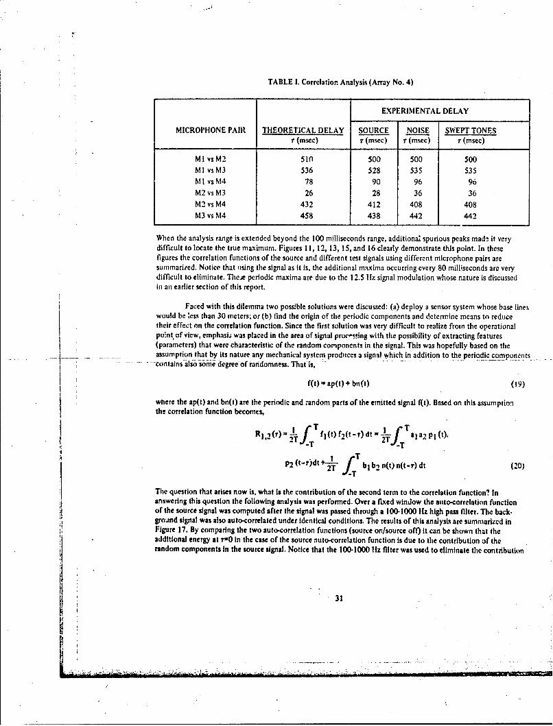
Table I summarizes the results of this correlation analysis. The discrepancies observed between theoreticaland experimental values of the delay times are believed to be due to the fact that the theoretical values werecomputed on the assumption that the terrain was flat. In actuality this was not the case. On the other hand, thedifferences observed between the calculated values of the delay times of the source and the test signals using thesame microphone pair are attributed to the fact that the test signals when played back into the system were physicallyseparated from the source by about three meters. That is, a maximum delay differcnce in the order of 8 millisecondsis pessible. This is well within the differences observed. This point clearly shows the resolution of the technique.The good agreement between theory and experiment demonstrates that a source of disturbance can be localizedwith a high degree of accuracy using correlation techniques applied over long base lincs.( 11 ) The computationssummarized here were performed using a Federal Scientific Correlation and Probability Analyzer.

From the above it should be noted that although in the analysis range between zero and 100 millisecondsno real difficulties existed in reducing excessive periodic components from the correlation function, in all cases itwas postible to produce the true correlation maximum. The real problem for larger delays is by far more complex.

23

....................

I ,'. I II I I

k j -

4 t 1 I II I

/

9

*1

9U

4'

a

___ .1 __

410

41

I.41

0 p5

UI.

- - U � b I - 0

zaoa�I'IdNY/zHIL

24

/ a ......../

IJ

(a)

rr

(b)

250 350 450 550 650 "-750'T1 2 (asec)

Figure II. Cross-correlation Function of MI vs M2: (a) source signal; (b) 40.80 Hz band-limited white noise;and (c) 40-1S2 Hz swept tones

i2

A- u

(b)

250 350 450 550 65015113 (U400)

Figure 12. Cross-correlation Function of M I vs M3: (a) source signal; (b) 40480 Hz band-limited white noise;and (c) 40-1 SOHz swept tones.

26

7

CC,(b

0 40 s0 120 160 200

Figure 13. Cross-orrclation Function of M I vs M4: (a) 40-80 Hi band-limited white noise; (b) 40-150 Hz

swept tones; and (c) source signals.

27

04

123 (2(0)

Figure 14. Cross-coffebtiton Function of M2 vs M3: (a) source signals; (b) 40-80 Ha band-limited white noise;and (c) 40-150 Hz swept tones

28

(b)

CIL

VW VV V

Em

0 100 200 300 400 500T24 (USOC)

Figure I S. Cross-correlatlon Function of M2 vs M4: (3) source signals; (b) 40-80 Hz band-limited noise; and(c) 40.1S0 Hz swept tones.

29

0 100 200 300 40050T311(lc

Figure 16. Cresa~orrelation Function of M3 vs M4- (a) source signals-, (b) 40413 Hz band-limited mble-, and(c) 40-150 Hz,4swept tone".

30

TABLE i. Correlation Analysis (Array No. 4)

EXPERIMENTAL DELAY

MICROPHONE PAIR THEORETICAL DELAY SOURCE NOISE SWEPT TONESi' (msec) 7 (msec) r (msec) r (msec)

MI vs M2 510 500 500 500MI vsM3 536 528 535 535M I vsM4 78 90 96 96M2 vs M3 26 28 36 36M2 vs M4 432 412 408 408M3 vs M4 458 438 442 442

When the analysis range is extended beyond the 100 milliseconds range, additional spurious peaks mad, it verydifficult to locate the true maximum. Figures 11, 12, 13, 15, and 16 clearly demonstrate this point. In thesefigures the correlation functions of the source and different test signals using different microphone pairs aresummarized. Notice that ,using the signal as it is, the additional maxima occurring every 80 milliseconds are verydifficult to eliminate. Thlee periodic maxima are due to the 12.5 Htz signal modulation whose nature is discussedin an earlier section of this report.

Faced with this dilemma two possible solutions were discussed: (a) deploy a sensor system whose base lineswould be ess than 30 meters; or (b) find the origin of the periodic components and determine means to reducetheir effect on the correlation function. Since the first solution was very difficult to realize from the operationalpo:nt of view, emphasi.b was placed in the area of signal proc.ssing with the possibility of extracting features(parameters) that were characteristic of the random components in the signal. This was hopefully based on the

S - - assumption that by its nature any mechanical system proditces a signal which in addition to the periodic components--contains also some degree of randomness. That is,

f(t) ap(t) + bn(t) (19)

where the ap(t) and bn(t) are the periodic and ;andom parts of the emitted signal f(t). Based on this assumptionthe correlation function becomes,

T TRI,20r)=/T f. fI(t) f2 (t-r)dt 2-T ala2 PI(t).

P2 (t-)dt+- 2T f blb2 n(t)n(t-r)dt (20)

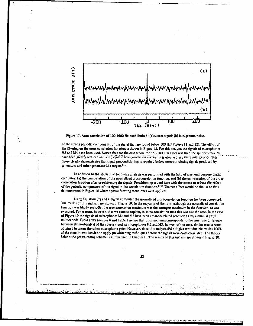
The question that arises now is, what Is the contribution of the second term to the correlation function? Inanswering this question the following analysis was performed. Over a fixed window the anto-correlation functionof the source signal was computed after the signal was passed through a 100-1000 Ilz high pass filter. The back.ground signal was also auto-correlated under identical conditions. The results of this analysis are summarized inFigure 17. By comparing the two auto-correlation functions (source on/source off) it can be shown that theadditional energy at 1=0 in the case cf the source outo-correlation function is due to the contribution of therandom components In the source signal. Notice that the 100.1000 Hlz filter was used to eliminate the contribution

4 •31

0E4

'44

200 1UU 'Th (Ins eC 1JU Luu

Figure 17. Auto-correlation of 100-1000 Hz band-limited: (a) source signal; (b) background noise.

of the strong periodic components of the signal that are found below 100 Hz (Figures 1I and 12). The effect ofthe filtering on the cross-correlation function is shown in Figure 18. For this analysis the signals of microphones

. . . M3 .and.M4 have been used. Notice that for the case where the 150.1000 Hz filter was used the spurious maximahave been greatly reduced and a dEzernible true correlationrn•aximiim is obscrved at t-438 milliscconds.-This---=---figure clearly demonstrates that signal preconditioning is required before cross-correlating signals produced bygenerators and other generator-like targets.(o0 )

In addition to the above, the following analysis was performed with the help of a general purpose digitalcomputer: (a) the computation of the normalized cross-correlation function, and (b) the computation of the cross-correlation function after prewhitenlng the signals. Prewhitening is used here with the intent to reduce the effectof the periodic components of the signal in the correlation function.(tO) The net effect would be similar to th-Atdemonstrated in Figure 18 where special filtering techniques were applied.

Using Equation (2) and a digital computer the normalized cross-correlation function has been computed.The results of this analysis are shown in Figure 19. In the majority of the runs, although the normalized correlationfunction was highly periodic, the true correlation maximum was the strongest maximum in the function, as wasexpected. For reasons, however, that we cannot explain, In some correlation runs this was not the case. In the caseof Figure 19 the signals of microphones M2 and M3 have been cross-correlated oroducing a maximum at 1-28milliseconds. From array number 4 and Table I we see that this maximum corresponds to the true time differencebetween times-of-arrival of the source signal at microphones M2 and M3. In most of the runs, similar results wereobtained between the other microphone pairs. However, since this analysis did ndt give reproducible results 100%of the time, it was decided to apply prewhitening techniques before the signals were cross-correlated. The theorybehind the prewhitening scheme is P,-mmarized in Chapter I1. The results of this analysis are shown in Figure 20,

32

S... . . .. .. ."" . ......... . .... . ... .... . .. iS - i 'i...... .. ' . ... .. . . ... . .... . .. .. . . . .. .. . .

(b)

(b)

54

( a)

I I

S.. .... (a )

0 100 200 300 400 500"N 1r34 (UmoC)

Figure 18. Cross-correlation Function of M3 vs M4 (Array No. 4) over the Analysis Range 0-500 msec. Band-

Limited Source Signals: (a) 100.1000 Hz; (b) 150-1000 Hz; (c) SO-1000 Hz; and (d) band-limited white noise160.320 Hz.

33

S. .. .. . ...... .... . .. '-

i-AtC-

2

N

00

Ua

* U

-3(V�

1-U

C

I-

S

�(�.)d zanZIIdNV

34

- ___________

I

- -- �*�-.� -

ILI

SC

-J C

21

In this figure the signals of microphones M2 and M3 used to produce Figure 14 were prewhitened an~d then werecross-correlated. In this case, as in the one above, the maximum at r=28 milliseconds is the true maximum andstands well above the spurious maxima. The analysis done with other pairs of nmicrophones using prewhiteningtechniques as a function of integration window is shown in Figure 21. In this fig'ire the correlation maximum iscentered over the analysis window. Using this technique all computer runs produced discernible correlation maxima.On the other hand notice that the periodic component has been greatly reduced as compared to Figure 10.

Once a workable correlation technique was established an attempt was made to locate the source usingdata that were obtained through an operational system (see Chapter 111). Although the IGLOO WHITE Phase IIIsystem filtered out most of the energy below 50 Hz because of a notch f'dter used at about 60 Hz (Figure 22), thecorrelation maximum could be found quite easily (Figure 23). Using the delay times (r) between different micro-phone pairs and Equation 8 one can solve for the coordirnates of the source. These results indicate that mechanicalsources whose main signal is highly periodic could be located using correlation techniques.

Notice that in addition to the method described in this report for identifying the generator-type targets,a technique based strictly on looking for the engine firing rate has been successfully ,eployed in SEA.P19) A briefdescription of this type of detection is given in Chapter III of this report. For more details see reference ! 9).

36

.L.11<;k

.33e

.3 (b)

.2.

0.0- ---

.- 4I IV

P3.3 .14 see .5 .

CL .3

.2.

.2

0.0

A - .3itq

Fiue2 .3Coscfeai ewe n M4, after Sina Prwieig saFntino6h nerto

Widw:()14sewno;()12sewidw c e idw d e idw

/3

C)

00

4 .00z

.1IM

380

CONFID","OTIAL

IGo

+ +1

399

CONFIDENTIA(This ~ ~ ~ 3. pa sacadld

CONFIDENTIAL

V. (C) Summary and Conclusions (U)

(C) This work was concerned with application of acoustic base line techniques to detection, identification, andlocation of enemy weapon systems powered by generators. An acoustic base line system locates by measuring timc-of-arrival of acoustic signals produced by the target of interest, in this case the generator, at three or more acousticsensors distributed in a relatively broad array. Such time-of-arrival (TOA) techniques have been used successfully inother applications. In this case, however, the long base line (acoustic sensor separation) and the highly periodic nature

of acoustic signals generated by the source lead to severe ambiguity in source location. The technical challenge in thiswork involved separation of the periodic components of the source signals and pr.ervation of the more randomcomponents for use in arrival time measurement and subsequent target location.

(C) Experimental woik was performed at Eglin AFB, Florida and was designed to provide information on allvariables of interest Including weather and interference. The sources used were:

1. Foreign generators

2. Pure and swept tones

3. Band-limited white noise

4. Explosions

5. Aircraft interference

6. Vehicles singly and in groups.

(C) Detection was performed using the following:

S.....--- -t. -Hard-wired microphones wired into an RADC recording facility.

2. Existing IGLOO WHITE system with Phase III modified commike collocated with RADC microphones.AD aspects of the experiment including design, instWllation, and operation of the instrumentation system wereperformed by RADC personnel with support from 3246TW, Eglin AFB, Florida.

(C) Subsequent to the field phase of the program, the data were analyzed at RADC using correlators, spectrumanalyzers, and digital data processing equipment. T.e results of the analysis successfully demonstrated thefollowing:

1. Detection and location of the source was possible over base line,.. of 600 meters by applying:

a. Signal prewhltening techniques; and/or

b. Stochastic correlation techniques.

2. Accuracies within a few moters were achieved under calm weather conditions.

3. Identification of the target was performed based on the modulation of the acoustic signal by the fundamentalfrequency of the source.

"40

CONFIDENTIAL

CONFIDENTIAL

(C) The technique described above provides an approach to remote monitoring of enemy lines of communicationsand fixed installations for tactical target interdiction and strategic purposes. The most important current example islocation of SAM generators in a jungle environment. Presently this type of source is very difficult to locate usingother detection techniques. This work not only provides a tool for accurately locating SAM generators withavailable hardware, it also prov"J!z the means for properly classifying the target.

I

41

CONFIDENTIAL

, REFERENCES

1. Faron, Jr., J.J. and Hills, Jr., R., "The Application t:fCorrelation Techniques to Acoustic Receiving Systems,"

Technical Memo No. 27 and 28, Acoustic Research Laberatory, Harvard University, Cambridge, Mass., 1952.

2. Goff, K.W., "The Application of Correlation Techniques to Some Acoustic Measurements,"./. Acoustical Soe

AM 27,236, 1955.

3. Lange, F.H., Correlation Techniques. lliffe Books Ltd., 1967.

4. Gilbrech, D.A., and Binder, R.C., "Portable Instrument for Locating Noise Sources i• Mechanical Equipment,'"£ Acoustical Soc Am 30, 842, 1958.

5, Jacobson, M.D., and Talham, R.J., "Use of Pressure Gradient Receivers in a Correlator Receivit:• System,"

Z AcousticalSocAm 31, 1352, 1959.

6. Jacobson, M.J., "Correlation of a Finite Distance Point Source," £ Acoustical Soc A m 31,448, ! 959.

7. Jacobson, M.J., "Space-Time Correlation in Spherical and Circular Noise Fields," £ AcousticalSoc Am

34, 971, 1962.

8. Bolt, Beranek and Newman, inc., "Signal Processing Techniques for Sound Ranging," Technical Reports

ECOM-0378-1, 1967; ECOM-0378-3, 1968; ECOM-0378-4, 1969.

9. Harris, J.R., "Study of Sound Location by Hyperbolic Fixing," NADC-SD-6814, 1968.

•I 10. Maloney, J.E., Sebastian, R.L, and Mathieu, K.F., "Evaluation of Atmospheric Correlation Techniques,"

SRADC-TR-72-179, 1972, AD 903 724.

S................................................. II. Constantine, J.G. and Dickimon• M:, "Long Base Line Acoustic CorrelationTechniques," RADC-TR:72.265• .......•: 1972, AD 906 705.

i! 12. Willow Run Laboratories, "An Investigation of Factors Affecting Sound Ranging; Literature Researchand

SAnalysis," The Institute of Science and Technology, University of Michigan, AD 698 565, 1969; AD 711 574,• ! 1970; AD 711 575, 1970; and ECOM-O0013-209, 1971.

L••i 13. Papoulis, A., Probability, Random Variables and Stochastic Processes, McGraw-Hill Book Company, ! 965.

* 14. Defense Special Projects Group, °'DSPG Systems Design Description," 20 August 1971, Secret, Group 3.

15. Fountain, L.S., "The Influence of Meteorological Conditions on the Propagation of Ultrasonic Energy in AirNear the Earth's Surface," Special Research Report, Southwest Research Institute, May 1962.

16. Fountain, L.S., Owen, E.T., and Vest, Wid, "Development and Evaluation of the Sonic Intrusion Detector,"Final Report, February 1969, AD 500 196.

17. Eydng, C.F., "Jungle Acoustics,",/. AcoustlcalSocAm 18, 257, 1946.

18. Torok, S.F., "Vehicle, Aircraft Classification Manual," Naval Air Development Center, NADC.72058-SD,

21 April 72.

"19. AFSC, E$11n AFB, FA, "Evaluation of Modified COMMIKE," Project Directive No. O!25AO01, Headquarters,

3246th Test Wing, 12 Mar. 72, •cret, Group 3.

43

, , i , , I i i I i I i' I I I I [ I I I I I I '

APPENDIX

The time domain correlation program was written in FORTRAN IV for use on a PDP-9 general purposedigital computer by RADC/DCTI. The correlation function is normalized (Eq 2) and printed out in integer format.A plot of the normalized correlation function can be obtained by a software plotting program.

The correlation program has the capability of handling 835 points per correlation. The resolution depends onthe digitizing rate of the data in conjunction with the 835 point per correlation.

The three-sensor target location program was also written in FORTRAN IV by RADC/DCTI. The arraygeometry and the time delays of the acoustic signatures of interest between the three sensors are needed for alocation.

The general equations used in the digital program for the three-sensor target !ocation using TOA are:

2 2 1/2 1/2V0 7 12 =(X0 + Y) - [(X0 -X 2 )2 +(YO-Y 2)

2 ] 1/22 0 2 (21)

V0• 13 (X0 + y() I/2 -[(X0 X3) 2 +(Y 0 .- 3 )2j 1/2o 0 (22)

whereV0 - speed of sound.

7 12 - Delay time for the acoustic signature of interest between sensor 1 and sensor 2.

r 13 - Delay time for the aco:!stic signature of interest between sensor I and sensor 3.

X0 , YO - Cartesian coordinates of the target locatic 2.

X2 , Y2 - Cartesian coordinates for sensor 2.

X3, Y3 - Cartesian coordinates for sensor 3.

The location of sensor I is at the origin of the Cartesian coordinate system, therefore X1 0 and YI 0.

Solving for the target location, the following equations are obtained:

X0 A + BR0 (23)

Y0 Al + B1 R17* (24)

where•, .(X2 + ,,2) 12(25)

An ,y:(X2+ y2)Y 2 ( Y32)y Y3(Vo 12)2+ Y2(Vov,3)2

B n Y3 (Vo' € 12 ) -Y 2 (Vo T 13)

X2 Y3 -X3 Y2

A.1

1'

Al X2(X2 y 2 ) X3V0 712) "X2X02 13)3 3 2 2 1(28)

2 (X2 Y3 X3 Y2)

BI = X2 (VOr 13) -X 3 (Vor 12) (29)

X2 Y3 - X3 Y2

Squaring equations (23) and (24), then adding the two equations together, the following quadratic solution for R0i3 formed:

R0 = J ± =Fj 4 NY. (30)

2N

whereJ = 2 (AB +Al b1 ) (31)

N = B2+ B12 _ 1 (32)

K = A2 + A"I2 (33)

As long as the target is witlin the triangle formed by the three sensors, a unique solution is obtained from equation(30). R0 is then substituted into equations (23) and (24) for the Cartesian coordinate of the target location relativeto sensor 1.

The block diagram of Figure 24 depicts the steps involved when signal prewhitening is used to reduce theperiodic structure of the correlation function. The taieory and equations used to develop the digital computerprograms for signal prewhitening are described and presented in Section II.C. Below is a description of the symbolsin the block diagram of Figure 24.

. -. .X (t), X2 (t) -Time varying functions

F1 (w), F2 (w0) - Discrete Fourier transform of X1 (t) and X2 (t) respectively.

F2 * (M) - Complex conjugate of F 2 (Mo).

K2 (w) - Prewhitening functions

FFT - Fast Fourier Transform

p 1,2 (r) - Cross-correlation function

WSF - Window Shaping Function (i.e. Hanning, Hamming etc.).

A-2

Lx1(t) x2 (t)

FFT FFT

F (W) F (w) F (2Ui)

PREWHITENING

b [SI 1 2 (w)*K2(w)] [FI~)F2II)*] WSF s.-

FFT-1

Fiue24. Block Diagram of Digital Prewhitening Technique as Applie to the CrowsSpect~atPower Density

A-3

C THREE SENSOR TARGET LOCATION PROGRAM.C ROME AIR DEVELOPMENT CENTER.C LT MARK D. DICKINSON (DCTI).CCC CALL INIT INITIALIZES THE TEKTRONIX 611 DISPLAY.

CALL INITC READ IN ARRAY DIIENSIONS AND TIME DELAYS FOR THREE SENSORS.101 FORMAT (F8.3)200 WRITE (4,100)100 FORMAT (38H DISTANCE BETWEEN Ml AND M2 IN METERS:)

READ (4,101) R12WRITE (4,102)

102 FORMAT (38H DISTANCE BETWEEN MI AND M3 IN METERS:)READ (14,10) R13WRITE (4,104)

1o4 FORMAT (34H ANGLE FROM R12 TO R13 IN DEGREES:)READ (4,101) TH13WRITE (4,106)

106 FORMAT (35H ENTER D12, D13 AND D23 IN SECONDS:)READ (4,300) D12, D13, D23

300 FORMAT (3F8.3)107 FORMAT (F8.5)C CONVERT TH13 FROM DEGREES TO RADIANS.

TH13=TH13*.01745C_ C. -- CONVERT TIME--DELAYS -FROM TIME-TO DISTANCE BY --------C MULTIPLYING BY THE SPEED OF SOUND.

D12=D12*344.D13=D13*344.D23=D23*344.X13=RI3*COS(TH13)Y13-RI3*SIN(TH13)

C THREE SENSOR TARGET LOCATION COMPUTATION STARTS HERE USINGC TIME DELAYS D12 AND D13.

A=((R12**2)-(D12**2))/(2.*R12)B=D12/R12AI=(XI3*((DI2**2)-(RI2*.*2))-RI2U((DI3**2)-(RI3**21)))/(2.'Rl2*Y13)BI.(D13*R12_DI2*X13)/(R12'Y13)ZAPaSQRT(((2.*(A*B+AI*BI))**2)-(4.*(BO*2+BI**2-1.1)*(A**2+AI**2)))RSI=(-2.*(A*B+Al1B1)÷ZAP)/(2.*(BO*2÷Bl**2-1.))RS2-(-2.*(A*B+Al*B1)-ZAP)/(2,*(B**2÷Bl**2-1.))IF(RS1.LE.0.) GO TO 103Xl=A1+BI*RS1YIuA+B*RS1THS1U(ATAN 2 (X1,YI))*57.29

AA4 -i

*.,7 7 j7 7 7 7 ~

/

C WRITE OUT DISTANCE FROM SENSOR ONE (Ml) TO THEC TARGET LOCATION IN METERS.

WRITE (8.,105) RS1105 FORMAT (21H+DISTANCE TO TARGET a, E114.5)C WRITE OUT ANGLE THS1 IN DEGREES FROM R12 TO RS1.

WRITE (8,109) THS1109 FORMAT (23H+ANGLE F'ROM R12 n2 ES=,E114.5)103 IF(RS2.LE.O.) GO TO 108

X2=Al+Bl*RS2Y2=A+B*RS2THS2=(ATAN2(X2,Y2) )*57.29WRITE (8,105) RS2WRITE (8,109) THS2

C THREE SENSOR TARGET LOCATION COMPUTATION STARTSC HERE USING TIME DELAYS D21 AND D23.108 IF(RS1.LE.0.AND.RS2.LE.O.,) GO TO 113

D21=D12R23=SQRT((R13**2)+(Rl2**2)-(2.*Rl3*Rl2*COSt:TH13)))TH21=ATAN2(Y13,(R12-X13))X21=Rl2*COS(TH21)Y21=Rl2*SIN( TH21)AP=(R23**2-D23**2)f(2. *R23)BP=D23/R23A1Ps(X21*( (D23**2)-(R23**2) )-R23*( (D21**2)-(R21W*2)1))/(2.*R23*Y21)BlP= (D21*R23-D23*X21) /( R23*Y21)ZAP=SQRT(((2.*(AP*BP+A1P*BlP)**2)-(4.*(B**2+

RSlP=(-2.*(AP*BP+A!P*Blp)+ZAP)/(2.-*(BP**2+BlP**2-1.))RS2Pm(-2.*(AP*BP+AlP*BlP)-ZAP)/(2.*(BP**2+BlP**2-1.)).rF(RS1P.LE.0.) GO TO 110THS1P=(ATAN2((AlP+B1P*RS1P), (AP+BP*RS1P)))*57.29WRITE (8,105) RS1PWRITE (8,201) THS1P

201 FORMAT (23H+ANGLE FROM R23 TO Rs-,E114.5)110 IF(RS2P.LE.O) GO TO 112

THS2P=(ATAN( (AlP+BlP*RS2P) ,(AP+BP*RS2P) ))*51 .29WRITE (8,105) RS2PWRITE (8,201) THS2P

102 IF(RS2P.LE.O.. AND.RS1P.LE.O.) GO TO 113GO TO i14~

113 WRITE (8,202)202 FORMAT (26H+No SOLUTION WAS OBTAINED.)114& PAUSE 10

IF(ISENSW(17).EQ.-l) GO TO 200* ~STOP

END

A-5

(This pazge Is unclassitied)

UNW SSiFiLb

C TIME DOMAIN CORRELATION PROGRAM.C ROME AIR DEVELOPMENT CENTER.C CAPT MIKE CRONE (DCTI)CC SUBROUTINE CORAL

COMMON iN(4,167o),NR1EC,NPC iN(~4,).670-WORKING ARRAY WHERE ROW 1 IS THEC FIRST CHANNEL OF DATA, ROW 2 IS THEC SECOND CHANNEL OF DATA AND ROWC 3 IS WHERE THE NORMALIZED CROSS-C CORRELATION IS STORED. THE ARRAY WILLC HANDLE 1670 POINTS PER ROW.C NREC.-NUMBER OF RECORDS.C NP=NUMBER OF POINTS.

B=ONP=NP/2DO 100 I1I,NPC-IN(1,i)

100 B=B+C**2DO 200 J=1,NPAl-OD-0DO 10 Kinl,NP

Ll-K+JR2uIN (2 ,Ll-1)-A,1-R1'R2+AI.

10 D-R2*02+D200 IN(3,J)-Al/SQRT(B*D)*2o4T.

CALL INITC CALL INIT INITIALIZERS THE CRT DISPLAY.

WRITE (8,150)150 FORMAT (30H NORMALIZED CROSS-CORRELATION-)

15WRITE (8,175) (IN(3,J),'=1,NP)15FORMAT (lH,l1o6)

PAUSE 1RETURN-END

A-6

L.~ ~ ~ cagq 's unC1l~