~-At~i 991 A NEW PUMPJET DESIGN TwEOAVAD) TETRA TfCN INC PASADENA 1/1CA 0 FURUYA ET AL 81 MAR 86 TETRAT-TC-3037WOO814-85-C-050

UNCLASSIFIED F/G 2t/5 WL

EhEEEEEEEmhhhIEhEEomhohhhhhhEsofflfflffllfllfllfllf

EhhhhE~hhE

L102

1111.25 1.6

MICROCOPY RESOLUTION TEST CHART

, l iL& II

Report No. TC-3037Contract No. N00014-85-C-0050

AD-A181 901

A NEW PUMPJET DESIGN THEORY

by LOKITSUGU FURUYA IWEN-LI CHIANG

TETRA TECH, INC.

* 630 NORTH ROSEMEAD BOULEVARDPASADENA, CALIFORNIA 91107

MARCH 1986 ELECTE

Prepared for

DAVID W. TAYLOR NAVAL SHIPRESEARCH AND DEVELOPMENT CENTER

• BETHESDA, MARYLAND 20084

OFFICE OF NAVAL RESEARCH

ARLINGTON, VIRGINIA 22217-5000

Approved for public release;distribution unlimited

87 6 30 22L

0

Report No. TC-3037Contract No. NOO014-85-C-0050

A NEW PUMPJET DESIGN THEORY

by

OKITSUGU FURUYAWEN-LI CHIANG

TETRA TECH, INC.630 NORTH ROSEMEAD BOULEVARDPASADENA, CALIFORNIA 91107

NTIS CR A&

DFIC TAB EJ

* MARCH 1986 E

D: t

0AMVlab,;ty CodesPrepared for

~~a j dj or0! t ' .% ,cl

DAVID W. TAYLOR NAVAL SHIPRESEARCH AND DEVELOPMENT CENTER

BETHESDA, MARYLAND 20084

OFFICE OF NAVAL RESEARCH800 NORTH QUINCY STREETARLINGTON, VIRGINIA 22217-5000

Approved for public release;distribution unlimited

UNCLASSIFEDSIRUITY CL.ASIFIuCA~T110 00 ?%is PAGE ("one O.e. ZndIrn

REPORT DOCUJMENTATION PAGE READ'O INSTRUCT-ONSI. IMPORT "14101111 GOVT ACCESSION NO . L ACIPIENr*S CATAkLOG NUMOCR

* TC-3037

a. ?169. (and Suhuef.11) L. TV" Or RXISORT a P.CpfOO COVEMIOTechnical - Theory & ExperimenJanuary 1, 1985 - Dec. 31, 1985

A NEW PUMPJET DESIGN THEORY S. PCRP11ORIG ORG0. REPORT MUMSCATC -3037

* 7. JT1~O(.j . CONTRACT OR GRANT NUMdC1I(e)

0. Furuya IN00014-85-C-005oW.-L. Chiang

9. PORIT1304O ORGANIZATION SIAME AND AOORESS 10- PROGRAM 1LE.4KdEMT. PqOJ (Cl' TASK(AREA 4 WORK UNIT NuM99RS

Tetra Tech, Inc.* 630 N. Rosemead Blvd.

Pasadena,_CA__91107 ______________

If. COMYROLIII.G OPWIC 'SAII AMO AOORESS M A& RPORT OATEDWTNSRDC March 1, 1986Dept. of the Navy 13I. NUMMOEN OF PAGESBethesda, MD 20084 I 76

11. mmOiTORING AGENCY MNM 4 AOORIESS(ft dlieefg Item Caft,1111101 01119.) IS. SECURITY CLASS. (01 (Ili riPeff)Off ice of Naval Research

800 North Quincy St. UcasfeArlington, VA 22217-5000 I~.CZCLASSiF.CATIONl OOWWGAOIN-

SC)490ULC

14. OsSTRIGU7.1oN STATCUEJ4T (.1 hl As eot)

Approved for public release; distribution unlimited

:7. OJSTRIIIIITION0 STATEMIENT (ed! tho ahae&a4t aetod In 3104& 20, 11 diIIbremt 1"eM ROPe,)

14. SUPP#.9EMNARY NOTES

Sponsored by the Naval Sea Systems Command General Hydrodynamic Research0 Program and administered by the David W. Taylor Naval Ship R&D Center,

Code 1505, Bethesda, MD 20084.

it. gay wGAOS (Ceinitnue onefl.Io adds 11 nleOC@fi and Idan#1i0 07 bleck nufflhe)

PumpjetStreamline Curvature Method

C Blade-through FlowBlade-to-Blade Method

4*. ASSTRACT (Cenotnua , n . aes ide SI .8e4.0 aid identfy~ ay 6,104i m~RUN )

The pumpjet is a unique fluid machine which utilizes retarded wake flow andproduces high propulsive efficiency such as 90%. The existing pumpiet design

* method is based on a simple two-dimensional graphic method which was used forpum~p design. As the demand for the speed of underwater vehicles increased inrecent years, the existing design method became inappropriate. Effort has beenmade to develop a new three-dimensional pump design method by combining a blade-through flow theory with blade-to-blade flow theory. Such a method requires

* .I" D '3 17 3I 147 3 10OIGO 0, I NOV iS IS O3SOLET9 UNCLASSIFIEDSN.~i'G4.6OISECuRITY CLAS5IP'.CATICN OF THIS 10A09("6 an~~ d& dnImtod)

UNCLASS IF IED%.4b(.U0M1*Y C).ASSIFICATIOM OF Th,5 PAGC(Wn "A Enet"64

20.,many supporting sub-theories to be developed. The foundation work for the

blade-through flow theory, i.e., streamline curvature method, three-

dimensional flow mapping technique, as well as two-dimensional cascadetheory has been established in this FY-85 GHR program. Future work for

completing sub-theories and incorporating such theories into a unifieddesign theory will follow.

UNCLASSIFIED

S[CURIoy C.ASSIFICATIOw Of ? i$ pAGzo( ten 0evs tn,.,E)

TABLE OF CONTENTS

Page

1.0 BACKGROUND......................................... I

2.0 OBJECTIVES .......................o.................- 6

3.0 METHODOLOGY SELECTION FOR A THREE-DIMENSIONALPUMPJET DESIGNo.... ... ...................... 73.1 REQUIREMENTS AND CANDIDATESo... too........... 73.2 COMPARISON AND SELECTIONooo.............. 9

4.0 SELECTED DESIGN METHOD--BLADE-THROUGH!BLADE-TO-BLADE METHOD.o . ... . .. .. .......... oo . . . . . .. 114.1 PUMPJET GLOBAL HYDR ODYNAMICS~oo.o..o 13

4.1.1 Calculation of Thrust Force... ..... 134.1.2 Relationship Between Pump Head

0and Thrust .... ... . .... . ... .... o .. ... 164.1.3 Power Cal ulation .. o~ ... ~. 174.1.4 Procedure of Calculatina Propulsive

Efficiency with Vl1(r), etc. givenand Spe meslse... o... . tso 18

4.2 BLADE-THROUGH FLOW ANALYSIS - STREAMLINE*CURVAREMTURDSMET~o D(SCM) .... o. 2].

4.2.1 Mathematical Formulation. o. 214o2.2 Solution Method...... . . . . . . . . .. .,,.. 274.2.3 Potential Problems of SCM for Hihl

Nonuniform Velocity Profile Due to

*4.2.4 Numerical Results..... o . . . . . ... oo. .. . 304.3 BLADE-TO-BLADE FLOW ...... ... . .. .o . . . .o.. . 31

4.3.1 Transformation.... . ..... .oo. ... o.o. . 314.3.2 Loadn Corection on Linearized

Cascade Theory.... ....... ... o.o .. .. ... .34

4.3.3 Leading Edue Correction on LinearizedCascade Theory.. ..... .. ...... o.oo.. .. 37

6.0 REFERENCES...... o. . . . .. .... .o.o. . ... o. . .. oooo. .. 43

APPENDIX CALCULATION OF HEAD LOSS COEFFICIENT K1 44

0i

6e

G

LIST OF FIGURES

*Paae

1-1 A typical pumpjet blade and shroud con-figuration 48

* 1-2 A typical meridional flow velocity (Vm)distribution for a pumpjet where V. is up-stream flow velocity 48

1-3 A typical load distribution in terms ofV9 3 for pumpjet rotor blade where V9 3 is

* circumferential component of the turnedflow velocity 49

1-4 Typical pumpjet rotor blade configuration,(a) top view and (b) upstream view 50

* 1-5 Typical Cp and CT curves for the designedrotor blade profiles and deformed rotorblade profiles, showing about 7.3% increaseof Cp (i.e., ACp = .0083) where the designJd = 1.311 51

• 1-6 Flow configuration for cascade 52

4-1 Flow chart of the selected pumpjet designmethod 53

4-2 Schematic diagram of pumpjet flow 54

4-3 Flow chart for calculation of the pumpjetefficiency 55

4-4 Meridional velocity at station Q ofFigure 4-2 56

4-5 Meridional velocit distributions atstations © and t6 of Figure 4-2 57

4-6 Calculated propulsive efficiency as functionsof RI/R B (stagnation streamline radius) withthe incoming flow velocity amplificationfactor, 97 = 0* 58

4-7 The same as Figure 4-6, except for 97 = 5 59

4-8 The same as Figure 4-6, except for 97 = 1" 60

ii

List of Figures (Continued)

* Page

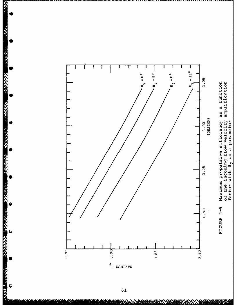
4-9 Maximum propulsive efficiency as a functionof the incoming flow velocity amplificationfactor with 07 as a parameter 61

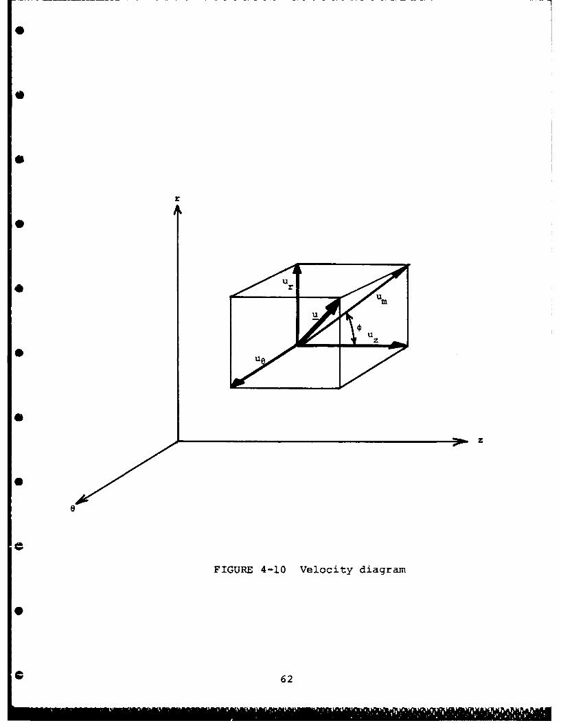
* 4-10 Velocity diagram 62

4-11 A schematic flow diagram used for numericalcomputations on Streamline Curvature Method 63

4-12 Calculated results of Streamline Curvature* Method for a typical underwater vehicle tail

cone with shroud where the solid lines are ofthe initial guess and dashed lines are theconverged solution (the dotted lines areq-lines used for the present computation) 64

* 4-13 Axisymmetric stream surface 65

4-14 Flow fie]d on the xy plane 65

4-15 Comparison of lift coefficient data, withoutmodification factor 66

4-16 Comparison of theoretical and measured liftcoefficient data for NACA 65-(15)10,81 = 45", a = 1.5 without modification factor 67

4-17 Comparison of lift coefficient data, with amodification factor of 0.725 applied to Cb 68

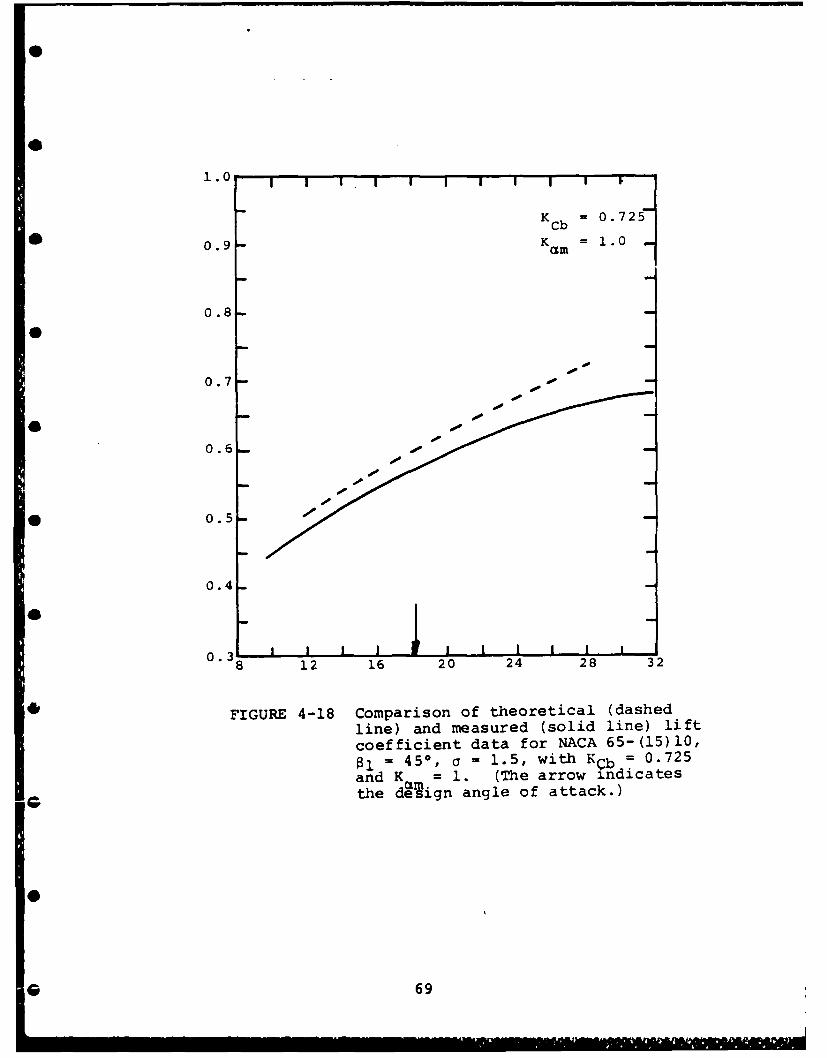
4-18 Comparison of theoretical and measured liftcoefficient data for NACA 65-(15)10,BI = 45", a = 1.5, with KCb = 0.725 and

SKam 1 69

4-19 Comparison of lift coefficient data, with(KCb, Kam) = (0.7, 0.75) 70

4-20 Comparison of theoretical and measured liftG coefficient data for NACA 65-(15)10,

81 = 45", a = 1.5, with KCb = 0.7 andKam = 0.75 71

4-21 Comparison of velocity distribution betweenthe singular perturbation method and test

* results of Herrig, et al. (1951) fora) NACA 65-(12)10, 81 = 45", solidity = 1.0,and al = 12.1" and b) NACA 65-(12)10,81 = 45", solidity = 0.5, and al = 7.3" 72

iii

M I N I A I116'11 1111111

1.0 BACKGROUND

The pumpjet is considered to be one of the most promising

candidate propulsors for high speed underwater vehicles and,

as a matter of fact, it has recently been employed for MK-48

torpedoes, ALWT--Advanced Light Weight Torpedo, now called

MK-50 and other underwater vehicles. The pumpjet

superiority over other propulsion devices is represented by

two major factors, i.e., high efficiency and quietness.

The pumpjet is one of few fluid devices which positively

utilizes retarded wake flow and produces high propulsive

efficiency. This peculiar situation may be understood

readily by considering the momentum equatin applied to a

control volume surrounding an underwater vehicle, fixed to6the inertial coordinate system. In the conventional pro-

peller, for example, the velocity of flow comng into a pro-

peller blade is approximately equal to the vehicle speed

since the propeller diameter is large enough to enjoy the

free stream flow. In order for the propeller to generate

any effective thrust, it should accelerate the flow, the

ejected flow speed being faster than the incoming flow. If

one observes this situation from the inertial frame, the

ejected flow has a finite positive flow speed against the

surrounding environment. It means that a certain amount of

the energy imparted on the fluid by the thruster is dumped

* in the surrounding water. On the other hand, the pumpjet

receives the retarded flow velocity, slower than the free

stream velocity. In order to generate a thrust, again this

flow should be accelerated. However, if the pumpJet is

c properly designed, the accelerated flow velocity can nearly

be that of the vehicle speed. If one looks at a similar

control volume, from the inertial f~ame, the ejected flow

out of the pumpjet has almost no absolute velocity and thus

• leaves hardly any jet wake after the vehicle passed. There

exists much less wasted energy in the flow field after a

vehicle with a pumpjet passes. This is the major reason why

...... 1

0

the pumpjet can produce such high propulsive efficiency such

as 90% or higher if it is properly designed.

Quietness is a guaranteed aspect with the pumpjet, as can be

seen from its configuration (see Figure 1-1); a long shroud

completely surrounding the rotor helps prevent rotor noise

from emitting into the outside flow field. Furthermore,

this "internal" flow machine has better resistance charac-

teristics against cavitation, resulting in quieter shallow

water operation where propulsors are most susceptible to

cavitation.

However, in order to achieve such a high standard of perfor-

mance there are many penalties to be paid in reality. The

first such penalty naturally stems from the pumpjet's util-

0 izing the velocity-retarded wake flow. A typical meridional

flow distribution at the inlet of pumpjet rotor is shown in

Figure 1-2; the velocity at the hub is only 30% of the free

stream velocity and rapidly increases to 75% at the shroud

internal boundary. This large velocity gradient in the

transverse direction is, of course, built up by the viscous

boundary layer effect and is one of the key features causing

difficulties in design, fabrication and eventually in

achieving the pumpjet high performance.

When one designs an axial or a near axial pump, it is cus-

tomary to distribute the blade loading from hub to tip in a

• forced vortex or a free vortex distribution method, such as

shown in Figure 1-3. Such distribution methods are impor-

tant in obtaining as uniform a discharge jet behind the

rotor as possible to minimize the mixing loss. However, a

0 serious problem arises in attempting to implement either

forced vortex or free vortex loading distribution against

the flow field having a large velocity gradient, as shown

in Figure 1-2. Due to the lack of enough meridional flow

velocity near the hub, the blade there should be designed

to have extremely large incidence angle as well as large

* 2

0

camber. It is f, r this reason that the pumpjet rotor

designed to date has a distorted profile shape from hub to

* tip, see Figure 1-4. If this were a conventional propeller,

the stagger angle would become smaller towards the hub and

the camber would stay more or less constant. However, for

the reason mentioned above, the pumpjet blade stagger angle

4 first becomes smaller up to the midspan area but becomes

larger toward the hub and thus the camber is designed to be

substantially larger.

This unusual rotor blade setup causes various hydrodynamic

problems. First of all, since a typical flow incidence

angle near the hub should be surprisingly high (e.g., 30"),

even a slight error in design may cause flow separation,

0 possibly cavitation and then noise generation. Secondly,

even if design is made properly, the same vulnerable

situation is generated with a slight flow disturbance or

blade deformation due to fabrication inaccuracy.* A recent

* study at Tetra Tech (see the report by Furuya, et al.

(1984)) indicated that some blade deformation, particularly

near the hub, could cause an increase of the power coef-

ficient, Cp, by as much as 7.3% (see Figure 1-5).

• Furthermore, there exists a profound discrepancy between

water tunnel test results and actual sea runs. What causes

such a discrepancy has not been clarified to date. It is

conceivable that I) a small trim angle (such as 1 - 2")

* existing at actual sea runs might have caused a change in

boundary layer velocity profile, or 2) the boundary layer

may be different between the water tunnel and unbounded flow

environment so that the pumpjet performance is substantially

affected. It should be noted that the utilization of the

boundary layer is an advantage in obtaining the pumpjet's

high efficiency on one hand but it is a disadvantage in

causing many difficult problems on the other hand.0

• Some pumpjet rotors are produced by investment castingprocess so that the fabrication accuracy cannot be

expected to be high.

3

The turning capability of the underwater vehicle thrusted

with a pumpjet is said to be inferior to that with, e.g., a

counter-rotating propeller. The reason for such inferior

turning capability seems also attributable to the utiliza-

tion of the wake flow; when the vehicle turns, the boundary

layer substantially changes. The pumpjet seems to lose a

considerable thrust capability due to the change of boundary

layer velocity profile, resulting in a poor turning capabil-

ity.

Another problem area in the pumpjet lies in the pumpjet

design method. The only design method developed to date and

used is a two-dimensional graphic method combined with

experimental data of Bruce, et al. (1977) despite the fact

that the pumpjet experiences a three-dimensional flow.

Based on the momentum theorem applied to the cascade con-

figuration, the blade sectional pressure increase Ap is

given

Ap = K VmoAVe (1.1)

where Ap = local pressure increase throughthe rotor,

• Vm = meridional velocity,

AV9 = circumferential velocity, and

K = a constant determined by thecascade configuration.

This two-dimensional momentum theory indicates that, in

order to generate a certain pressure increase at a blade

section, only the amount of total flow deflection in the

circumferential direction (between the inlet and exit)

counts, see Figure 1-6. In this method once the sectional

blade leading edge and trailing edge angles are determined,

then the rest of the blade section can be arbitrarily deter-

* mined by connecting these predetermined leading and trailing

edges, e.g., anglewise smoothly.

4

One of the obvious problems in this graphic method arises

from the fact that the flow coming into the cascade nlade

cannot exactly follow the blade camber, but substantially

deviates from it. What is required therefore is a camber

correction, the amount of which depends upon the cascade

geometry. Unfortunately, a typical pumpjet solidity* near

0 the hub is larger than 2.0 and therefore the camber correc-

tion required there becomes as much as 5 times in terms of

lift coefficient. It means that the camber graphically

constructed should be deformed until the lift coefficient

0 increases by 5 times that graphically obtained. This

correction is made semi-empirically based on limited numbers

of existing experimental data for cascade blade rlows. In

this sense, therefore, this graphical method is useless for

6the blade design near the hub and it can be said that the

final design is almost entirely dependent upon these empiri-

cal data.

0

a

* * Solidity is defined as a ratio of blade chord length toblade spacing measured normal to the axial direction andthe high solidity means more blade packed cascade.

0

2.0 OBJECTIVES

The objectives of the work to be conducted under the GHR

program are therefore:

1) to develop a more reliable and accurate pumpjetdesign method based on a three-dimensional pump or

* propeller design theory and then

2) to improve the pumpjet performance characteristics.

The characteristics to be improved include:

* a) the susceptibility to flow disturbance and rotor'sdeformation due to fabrication inaccuracy,

b) the discrepancy problem between the water tunneltest results and high speed sea runs and

* c) the poor turning capability.

0

0

0

G 6

mo m " - y'+ + ,~+ .+ \

0

3.0 METHODOLOGY SELECTION FOR A THREE-DIMENSIONALPUMPJET DESIGN

3.1 REQUIREMENTS AND CANDIDATES

There exist several possible approaches which can incor-

porate three-dimensionality into pumpjet design procedure.

However, the following aspects should be considered in

selecting such a methodology:

1) Moderate three-dimensionalityA pumpjet is usually installed astern of under-water vehicle hull where the hull shape has a

* negative slope of tapering shape. Although thisprovides three-dimensional flow characteristics,its three-dimensionality is rather mild, unlikethat in radial pump cases.

2) Capability of determining detailed blade profile4shapes as well as pressure distribution

In the previous two-dimensional graphic methodBruce, et al. (1974), the blade profile shape wasgraphically determined for meeting the headgeneration requirement. It is mainly for thisreason that the method failed to check the possi-bility of flow separation after the blade wasdesigned. A new method to be developed in thisresearch work should be the one with which thedetailed pressure distribution or velocity distri-bution on the blade can be determined.

0 3) Accurate loading determination supported byexperiments

When the sectional loading is determined analyti-cally in the course of designing a pumpjet, it isusually quite inaccurate since such loadingsubstantially changes due to the effect of adja-cent blades. It is therefore necessary for thenew method to incorporate the cascade effect intodesign procedure, or to use an empirical approachto increase such accuracy.

c With these features taken into consideration, the following

three candidate methods are compared in Section 3.2:

Method It Katsanis' Quasi-Three-Dimensional Method

* Method II: Blade-Through Flow with Blade-to-BladeFlow Method

Method III: Singularity Distribution Method

7

for which simple explanation will be given in the following.

Method I: Katsanis' (1964) Quasi-Three-Dimensional Method

In this method it is first assumed that a mean stream

surface from hub to shroud between blades is known in

advance. On this stream surface a two-dimensional solu-

* tion for the velocity and pressure distributions is

obtained. Then, an approximate calculation of the blade

surface velocities is made. This method is based on an

equation for the velocity gradient along an arbitrary

* quasi-orthogonal rather than the normal to the

streamline. Since the solution is obtained on this

quasi-orthogonal line, in this method, an iteration pro-

cedure needed in the previous orthogonal-line methodscan be eliminated and a solution can be obtained in a

single computer run.

Method II: Blade-Through Flow with Blade-to-Blade Flow

Method

The blade-through flow is first obtained by, e.g.,

Streamline Curvature Method (SCM). Once the stream sur-

face is found, it is mapped to a two-dimensional plane

* so that the blades cut through by the stream surface

become a row of blades, i.e., cascade on a plane. On

this cascade configuration, the blade-to-blade flow will

be solved. Difficulty in doing this lies in the fact

• that the governing equation is not a Laplace equation

any more on this two-dimensional plane, but a Poisson

equation due to the deviation of stream surface from a

perfect cylinder. In order to account for such

deviation into the two-dimensional flow, appropriate

source/sink and vortices should be distributed over the

entire flow field. This, in turn, results in the change

of blade camber shape. The design procedure relies on

an iteration scheme.

w8

Method III: Singularity Distribution Method

The method is similar to that used in design of conven-

* tional propellers, see, e.g., the work by Kerwin and

Leopold (1964). The differences in velocities between

the pressure and suction sides of rotor blade can be

represented by distributions of singularities such as

* source/sink and vortex. The strengths of such singu-

larities are determined by satisfying the boundary

conditions on the blade surface as well as those at

infinity. The methodology is described in the paper of

Kerwin and Leopold (1964) in detail.

The disadvantage of the method lies in the computational

complexity and instability. Furthermore, this type of

* method is suitable for design of devices used in the

open field, but not so for those used in the internal

flow since it does not take advantage of confined flow

configuration available for the latter case.

3.2 COMPARISON AND SELECTION

Table 3-1 provides qualitative evaluation on three candidate

methods described in the previous section over various

hydrodynamic, numerical and design aspects. As seen from

this table, a combination of blade-through method with

blade-to-blade flow seems to have an advantage over the

• other two methods. Particularly, the method has the capa-

bility of determining detailed blade profile shape as well

as loading and velocity/pressure distribution with accuracy

verified by existing cascade experimental data. It is for

this reason that the blade-through flow with blade-to-blade

flow method has been selected as a basic concept for devel-

oping a three-dimensional pumpjet design method.

Similar methods already exist for design of quasi-axial

pumps and compressors. However, those methods have many

inadequate features in their design procedure. Furthermore,

9

it is assumed in these design methods that the incoming flow

is more or less uniform, unlike the pumpjet where the rotor

should be designed for highly retarded velocity distribution

due to viscous boundary layer on the hull. The following

section describes the blade-through flow (BT) with blade-to-

blade flow (BTB) method with various aspects of modifica-

tions and improvement necessary for developing the pumpjet

design method.

10

@1

4.0 SELECTED DESIGN METHOD--BLADE-THROUGH/

BLADE-TO-BLADE METHOD

* Design of a pumpjet for an underwater vehicle requires pre-

liminary information on the vehicle including its geometry

and hydrodynamic drag coefficient. Furthermore, most

importantly, the velocity profile at an upstream reference

* section should be obtained either analytically or

experimentally. Any error in the velocity profile would

result in a pumpjet of lower efficiency or failure of the

pumpjet meeting the specifications at the design point. In

* the present study, it is assumed that this velocity profile

is given at a goal speed or at the corresponding Reynolds

number.

* The first step for design of a pumpjet (see Figure 4-1) is

to determine the shroud intake diameter. From the viewpoint

of cavitation, the maximum and minimum shroud diameter to

prevent cavitation must exist. If it is too large, the

* rotor blade tip speed becomes too high so that cavitation

occurs. On the other hand, if it is too small, the rotation

speed must be increased to generate the required head so

that the chance of cavitation inception also increases.

* Another aspect of determining the shroud diameter stems from

consideration of the overall propulsive efficiency. The

equation for global momentum balance should be able to

determine an efficiency-optimum shroud diameter for the

* given velocity profile and vehicle drag. The detailed

mathematical formulation and sample calculations will be

given in Section 4.1.

cOnce the shroud diameter is determined, the streamline will

be calculated by using the streamline curvature method

(SCM). In this calculation, the loading distribution on the

rotor and blade thickness must be assumed in advance. One

* of the major concerns in using the existing streamline cur-

vature method lies in the fact that SCM may only be used for

relatively uniform incoming flow, but may generate a sub-

C ii

stantial error for a thick wake flow, i.e., highly retarded

flow due to the viscous boundary layer on the vehicle hull.

* Detailed mathematical formulation and sample calculations

are presented in Section 4.2. Also included are discussions

regarding the problems of application of conventional SCM to

the thick wake flow.0

The next step of the design method is to map the stream tube

or surface calculated by SCM onto a plane so that the rotor

blades are mapped into cascade configuration. If the stream

* surface is totally cylindrical shape, the governing equation

to be used for the cascade analysis will be a Laplace

equation. Unfortunately, the stream surface is of three-

dimensional cone shape in general for the tail cone section

• of the underwater vehicle. The field governing equation now

becomes a Poisson equation, for which the results of power-

ful potential theory analysis are no more applicable. A

method of correcting the effect of the Poisson equation on

• the potential theory results is introduced to modify the

blade profile shape obtained in the potential theory. In

choosing the blade profile shape, the experimental data are

used to ensure that there is no chance of flow separation

0 due to overloading on the blade. Furthermore, based on the

calculated velocity along the blade, the cavitation incep-

tion is checked. If there exists a chance of either flow

separation or cavitation, the loading distribution from hub

0 to tip should be changed. If such a change is made, and/or

thickness of blades is changed, the streamline curvature

method should be used again to determine the new location of

streamline or stream surface. This iterative procedure will

be repeated until an overall convergent solution is

obtained. Section 4.3 describes the technical approach to

be used for the blade-to-blade flow analysis.

C 12

0t

4.1 PUMPJET GLOBAL HYDRODYNAMICS

It is a well-known fact that the pumpjet utilizes the tail-

cone low-energy, boundary layer flow in order to achieve its

high efficiency. It means that the optimum* pumpjet design

depends entirely upon the incoming flow velocity profile.

0 Figure 4-2 shows a schematic diagram of an underwater

vehicle tail cone/pumpjet flow. Q and 7 in Figure 4-2

are considered to be the upstream and downstream reference

stations, respectively, where it is assumed that the free-

stream static pressure exists, whereas 2Dand 0 are the

rotor inlet and exit stations.

4.1.1 Calculation of Thrust Force

The thrust force, T, due to the pumpjet work can be deter-

mined by applying the momentum equation to the control

volume enclosed by stations Q, and the stagnation

* streamline (see Figure 4-2).

T = rT7 d; 7 V 7(r)cose 7 rf r T 1 d; I V1 (r)cose1

SrH 7 H

(4.1.1-1)

where d;m7 = p2wrV 7 (r) cose 7 dr

((4.1.1-2)

di = p2wrV 1 (r) cose 1 dr

, I(r), V7(r) = midional, respflow velocities at and

V 1 (r),~ V7 r, respectively.ana I, 97 = m ridional flow angles at Q and

(sJ, respectively.

Note *By "optimum" pumpjet design it means that of provingthe maximum propulsion efficiency.

G 13

Therefore

T rT wr (r)cos 29 d Ip2irV 2(r)cos 2 adr

* rH7 rHI(4.1.1-3)

Defining the following quantities,

- rT 7/

r H7/ArB Vc rB

* Tl 1/r 8 = cosord(o)

v 1 r Hi/r 6 (B C)) ± 1 (4.1. 1-5)

v W f rT r B V 1 (r) rB c sr Hl/AB rWF- 1 (r-

and normalizing T, Eqn. (4.1.1-3) becomes

CT = T

rf T p27rrV 2 (r) co 2O a dr - jrrT p2irV1 (r)cos 2e9dr

r H7 1 H

f 2

r /HAB 2B

r A 2

r HI /rB (B~) (() OS.

G 14

(-, T_ CS7Cosai)Cm (4.1. 1-6)

where the mass conservation equation below has been used;

Cm =C m=C m7 (4.1. 1-7)

= Jf ~lp2rV 1 (r~cose1I dr(41*-8rHl

;7= 3'r p2wrV 7 (r) Cosa 7 dr (4.1.1-9)rH7

* r /r

Cm=- Ti B V 1(r) rC ml 2 = 2r cosae1BV;r Hl /rB8 V .(B

(4.1.1-10)

* r /r

Cm7 M7 2 fT7 B V7(r) r O 7*d

pV.;frr B r H7 /rB r. dk

Let's define

Aa V7 CO9 Vi 1 oa (4.1.1-12)W V

then we obtain, from (4.1.1-6)

CT =2 * W .* (4.1. 1-13)

Note that

in 2 (4.1.1-14)

where

re 15

T1 1rr~l/r I )Cosa 1 d

V CV V,) I LV1 r HI/AB (r)(4.1. 1-15)

f (j7) Cossld (f-SHl/rB \BIV

4.1.2 Relationship Between Pump Head and Thrust

The hydraulic head of the Pump HR is given

21frT 3 U V 3 'r 1 dIHR r H3/rB 8 .V V B Coa 3 B)

* y~g= r 3/rBV rBd ) (4. 1.2-1)

r H 3/Ar V0 r BcasI (B

where V3(r), Va3(r) =meridional and circumferential veloci-

5 ties at station T, respectively.

With the hydraulic efficiency riR introduced, the actual headgenerated in the fluid is ,

H = TIR H R (4. 1.2-2)

where H can be defined

) 2 22

H 2 (7 ) - (h) K1('.i) (4. 1.2-3)

(V. r 7 /B

where r\~ T7 /rB 76 ( (4. 1.2-4)

H.7/ B 8r

O 16

-2 f Cos CO~ d(jIV,\ r Hl/rB LiV , , rBI Fr (4. 1.2-5)

f T ( V1(r) r Cos

r AIt .F- cas

K, h ad loss coefficient between station Iand7~ (but mostly inlet loss and see Appendix

for determining K1).

Since

AVM V V7 -V 1 (4.1.2-6)

0 and AV m can be approximated as AV m V 7~ V1, Eqn.

(4.1.2-3) becomes

2V V ( AV V1)K(')C V (4. 1.2.7)V OD/2g cci

From Eqns. (4.1.1-12) and (4.1.2-7),

0- AV V (os Cs-a +. (cas 1 7 o

AV V V (4. 1.2-8)

*4.1.3 Power Calculation

The power to be used on the pumpjet rotor shaft can be

calculated by integrating the product of the local head andthe local mass flow rate over the entire duct flow,

P = f pgAQH,or in terms of the power coefficient

0 ~C - ____ f- Q

21 cA pV irrB

17

Pg f r 3 *93 'U.V (r)2rr 1osg3r H3 g dros

3 2

fpV OD irr B

or

rT3 3 /r BCP ~t e 3 (V ()V3 r)r c1 g

r H3/rB iL B e 8

(4. 1.3-1)

From (..-)

H HR f3 r 1 d= 2 r 8 V~ rB Cos d

P V C 2g rH3/rB G 3 B

HR C

V C/2 g

or

C Z HM (41.C2P R V0./2g m(4132

Therefore, the propulsive efficiency flp can be calculated

from the following definitions

=CT (4.1. 3-3)TP =

c4.1.4 Procedure of Calculating Propulsive Efficiency with

V1(), tc. given and Sample Results

Now all tools for calculating the propulsive efficiency flp

with V1(r) given are provided. The principal equations to

* be used will be Eqns. (4.1.1-13), (4.1.2-6), (4.1.2-8),

rW 18

(4.1.3-2), and (4.1.3-3). A flow chart describing the

calculation procedure is given in Figure 4-3.

Sample velocity profiles, Vl(r) and V2 (r), are shown in

4 Figures 4-4 and 4-5. The flow angles, e1, e2 and 97, can be

obtained from the drawings of a typical underwater vehicle

tail cone profile. The head loss coefficient, K1 , can be

calculated from the formula given in Appendix A with the

velocity distributions and pressure distributions both at

stations Q and ®, which are also given in Figures 4-4

* and 4-5.

Figures 4-6 to 4-7 show the results of calculations made for

various parameters, including the shroud opening diameter,

rl/rB, the exit jet flow angle 97, and flow velocity ampli-

fication factor. The design values of rl/r B and flow ampli-

fication factor are known, i.e.,

(rl/rB) D = .93.

Flow Amplification Factor = I

but that of 97 is not known except for the fact that the

average geometric angle of the shroud and tail cone angle at

6 exit is about ll. Theoretically, however, the jet coming

out from the shroud exit with ll" should align itself in the

direction of the body axis, indicating that 97 could be

zero. The present calculations were therefore made for

97 = 0", 5", 8" and ll'.

The shroud opening, rl/rB, was also varied in the present

analysis in order to determine the optimum shroud opening

Qradius in terms of efficiency. Also changed was the

incoming flow velocity amplitude to investigate a possibil-

ity of pumpjet efficiency improvement in combination with

the tail cone flow pattern change.

The pump hydraulic efficiency nR for this type of pump, used

in the analysis, is about 89", which is the measured value

by many pump makers.

19

0

Figures 4-6 to 4-8 show the calculated propulsive efficien-

cies as a function of the shroud opening rl/rB with the flow

* amplification factor as a parameter for 97 = 0", 5" and II',

respectively. As can be seen from these figures, the effi-

ciency curve has the maximum value at an rl/r B value spe-

cific for the conditions used.0

Figure 4-6 shows that the efficiency at the design condition

should be 88.4% when 97 = 0* is assumed. The design shroud

opening, rl/rB = .93, is slightly on the smaller side than

* that for the maximum efficiency. The maximum efficiency of

88.8% can be obtained at a slightly larger shroud radius.

i.e., rl/rB = .95. Also seen from Figure 4-6 is the faL.t

that the smaller the incoming flow velocity, the larger the

* maximum propulsive efficiency. This indicates that, if the

incoming velocity amplitude at the tail cone area can be

reduced by some means, the propulsive efficiency of the

pumpjet is substantially increased.

It should also be remembered that the actual efficiency

achieved is 76.9%, much lower than any of the values calcu-

lated here.

0As 97 increases, the efficiency curves shift to the lower

efficiency side, see Figures 4-6 to 4-8. This is naturally

expected since the jet thrusting force is not effectively

utilized as 97 increases.

It may also be coincidental, as seen in Figure 4-8, that if

97 = l1* is used as obtained from the pumpjet exit geometry,

the current shroud opening, rl/rB = .93, is the optimum

selection for providing the maximum efficiency, 82.9%,

smaller than that of the original design. It should be

pointed out that if 97 = 11" is the true exit jet flow

angle, an increase in the shroud radius for alleviating the

flow separation problem may cost a substantial efficiency

loss (see Figure 4-8). On the other hand, if 97 = O" is the

true value, a moderate increase (e.g., 2%) in the shroud

20

1111111~~ 1 -.11hW

S

radius will increase the efficiency in addition to the effi-

ciency gained due to the suppression of the flow separation.

0 However, again the penalty exists when the amount of shroud

radius increase exceeds more than 4%.

Figure 4-9 summarizes the present calculations in terms of

the maximum propulsive efficiency with e7 and the flow

amplification factor as parameters. It is shown that a

substantial efficiency improvement may be achieved by

1) reducing the incoming flow velocity amplitude0 by modifying the tail cone profile shape and

thus changing the boundary layer flow,

2) choosing the optimum shroud opening radiusdepending on the flow conditions (see alsoFigures 4-6 to 4-8),

3) redirecting the jet flow at the shroud exit asclose to the body axis as possible, if thejet flow of the current design is not.

* 4.2 BLADE-THROUGH FLOW ANALYSIS - STREAMLINE CURVATURE

METHOD (SCM)

4.2.1 Mathematical Formulation

* From the definition of entropy, S, in the second law of

thermodynamics, the following relationship is obtained for a

reversible transformation, i.e.,

TVS = VQ (4.2.1-1)

where T is the temperature and VQ is the amount of heat the

system under consideration receives, On the other hand, the

Q first law of thermodynamics says

VE = VQ + VW (4.2.1-2)

where E is the internal energy and W is the work performed

*Q on the fluid. Since VW = -pVv, (4.2.1-2) becomes

VE : VQ - pVv

G 21

0|

- VQ - pV(!) (4.2.1-3)

* where v is the specific volume of fluid and, in terms of

fluid density, p, v = 1/p. The definition of enthalpy, H,

is given by

12• H = u + E + -+ (4.2.1-4)p

where u is the amplitude of flow velocity and V is the

potential energy. Gradient of H yields

2VH = V(1 u + P) + VE + Vp + pV(1)

From the above equation and Eqn. (4.2.1-3),

2 1VH = TVS + V( u + P) + 7VP (4.2.1-5)

The steady-state momentum theorem gives

pu • Vu = -Vp - p VP (4.2.1-6)

where an assumption has been made that -VP = F, where F is

an external force. By using a vector identity, u x (V x U)= 1 V u2 - U . Vu, Eqn. (4.2.1-6) is now written

7416 2

ux (Vxu) = . Vu + VV + P Vp2

2or U x W = V (U+ J) + p (4.2.1-7)

where w = V x u. Substituting Eqn. (4.2.1-5) into (4.2.1-7)

gives

u x w = VH - TVS, (4.2.1-8)C

a relation first found by Crocco (1937), which will be used

to derive the formula used for SCM hereafter.

* By using the cylindrical coordinate system (r,e,z), the

velocity components of u are defined by

U= (ur, us, Uz). (4.2.1.9)

* 22

Thus, the components of vortex term w is written

(a) r =Vx u)r = (J --

au au(b) w9e = (V x u) e -=z r (4.2.1-10)a =Tz-- ar

jalru , aU r)-z z rVar - aT-

By introducing a direction m, defined by, (see also Fig.

"* 4-10)

(a) dm : dr : dz = um : u r : u z

2 2 2

(b) um ur + uz

(c) tan 4 = Ur/Uz (4.2.1-11)

(d) u r = um sino

(e) u z u m cost

it becomes evident that the m-direction is the 'meridional

direction" or on the projectirn of streamline in the r-z

plane. The directional derivative with respect to m then

becomes

(a) um : Ur r + amam r3r Zaz

(b) a ar a +az aam - am ar am az

sin L- + cost a (4.2.1-12)

8 r + az

where (4.2.1-11) has been used.

Furthermore, the e-component of the Crocco equation

(4.2.1-8) gives

u z (duz Bru 9 r ar au-ru

I

23

I /aH _ 39! (4.2. 1-13)

* Under the assumption of axisymmetricity,

~j0

T S= 039

so that Eqn. (4.2.1.-13) becomes

au r au z ru 9 3ruur e- ze- 1Ur a3r- z F

or 1 a (u 2 + u2) =u 8ru 9

2 To r z m 3m

Using (4.2.1-l1b),

3 m aru 9(4.2. 1-14)TO 3 -m

It is now ready to perform a coordinate transform of Eqn.(4.2.1-10) by using Eqns. (4.2.1-11), (4.2.1-12) and

(4.2.1-14). The result is

*(a) w= (Vxu) r an r e a - sino amua

*(b) w (Vxu) 1 2m~s [u in( au 3

(4.2. 1-15)

-coso ) - .

(c) W (Vxu)z 1[Brue - i 3ru 9 ur cos43O

*where rm is the radius of curvature of the meridional

streamline projection, defined by

* 24

(4.2. 1-16)r m am

*Further application of axisymmetricity to Eqn. (4.2.1-15)

yields

(a) r = (Vxu) ~~(re

(b) we = (Vxu) -- 1 2mOS taUrn n k m.

* (4.2. 1-17)

r m 2 ar]

* _ 1 1 aru(c) !z =r I

where the following relations

800

have been applied.

The right-hand side of Eqn. (4.2.1-8) becomes VH under the

assumption of adiabatic process for the fluid to go through

the pump channel.

Now, it is ready to write the r-component of Eqn. (4.2.1-8)

for the meridional flow velocity and the final form is shown

after some rearrangement:

aU+2 ' 2n _ __

Au 'u m + cosO)UlU am2Ai

8r/ am ru

=2 13 u. 3r 0 (4.2.1-18)

Eqn. (4.2.1-18) can he written as

0 25

0

au,m + P(r) u2 T(r) (4.2. 1-19)8r m

where

P(r) = 2 CO Io

um am+ rm)

T(r) = 2 1 -H r ar u2V7 r a rc42.-0

* In Eqns. (4.2.1-18) - (4.2.1-20), the first term of P(r),

i.e., sin/um • aum/am, will provide some difficulty in

numerical computations since it is related to the deriva-

tives with respect to "m". The basic philosophy of the

* streamline curvature method is to express the meridional

velocity in terms of hrl and "r-derivatives" so that um can

be solved in the direction of r only. This feature will be

of advantage in numerical computations since the derivatives

* with respect to "in" are not needed and thus the m-

directional control points do not have to be taken in fine

increments. Fortunately, sin /um • 3um/am can be expressed

in terms of r by using the continuity equation

au z + i arLr + = .

az r ar r ae

Again, applying the axisymmetric assumption and Eqns.

* (4.2.1-11), (4.2.1-12) and (4.2.1-16), the following rela-

tion is obtained

.sintO au~ - sin2p, (, + r + tan§-2kum am r rm COSt Br

(4.2.1-21)

The basic equation for the streamline curvature method,

* i.e., Eqn. (4.2.1-18), is expressed in terms of "r" except

for the radius of curvature, rm, so that it can be readily

solved numerically. The only problem remaining is that

26

um(r) cannot be uniquely determined. This problem can be

resolved by applying the mass conservation equation

2w f Kb. pr um(r) cosq dr = (4.2.1-22)rh

* where Kb is the blockage factor due to the blade displace-

ment thickness as well as that of the boundary layer, and Oq

is the angle between the line of integration (calledUq-line"' hereafter) and the line normal to the streamline.

* With this, the mathematical formulation for the streamline

curvature method (SCM) is completed. In what follows, the

numerical solution method for SCM will be described in

detail.

4.2.2 Solution Method

Since Eqns. (4.2.1-18) and (4.2.1-22) are highly nonlinear

for Um, only an iterative procedure depending on numerical

analysis is a possible solution method. First of all, it is

assumed that the distribution of upstream flow velocity is

known as function of r. Figure 4-11 shows a sample flow

configuration on an underwater vehicle tail cone where the

upstream location in this case is identified by station 1 (I

= 1). The upstream flow velocity can either be uniform or

nonuniform*. Station 1 is then divided into a finite number

of control points including the hub and the inside wall of

the shroud. In Figure 4-11, a total of 6 control points

(J = 6) are used. By using the mass conservation equation

(4.2.1-22), the local mass flow rate (gj, 3 +1 ) between each

two adjacent control points 3 and 3+1 is calculated. The

total mass flow rate, C1 , is just the summation of local

flow rates

*Note) However, the upstream flow, which is severelyretarded or highly nonuniform due to, e.g., theviscous effect, may present problems of accuracy,which will be discussed in Section 4.2.3.

27

= ,(4.2.2-1)

* r3~

where 2 ir fJ K or u(r) cosq dr (4.2.2-2)w lJ1J+l 2 f b r qr

For Stations I = 2,3,4..., the initial control points and

initial um velocity profile are also needed for the itera-

tion procedure. For the case of handling a uniform upstream

flow velocity, the selection of control points, J = 1 - 6,

and determination of initial flow velocity may be done in

the same manner as that for the first Station, I = 1, since

the constant velocity distribution can be assumed. However,

the case of nonuniform flow velocity distribution will

0 require a little care for selection of control points and

determination of initial flow velocity distribution. Among

many possible ways, it has been decided herein that the

velocity distribution is assumed to have a similarity nature

• as that of the upstream at I = 1, i.e.,

UmI (r) = k IUml (r)

r-rHIr 1= HI + rI-rHlrs-Hi (rlr±

; I = 2,3 .... (4.2.2-3)

where

rs1 , rSi = radius of shroud internal wall at Station 1and I (2 2), respectively

rH19rHI = radius of hub at Station I and I (a 2),respectively

kI = an arbitrary constant, dependent of Station I,to be determined later.

An arbitrary constant kI is used to adjust the total flow

rate at Station I 2 2 becomes G1 when umi(r) is substituted

into Eqn. (4.2.1-22). Once kI is properly determined, the

control points J = 2,3... can be determined by using Eqn.

G 28

(4.2.2-2). In order to carry out the above computations,

should be known in advance. If the control points at every

0 control station are known, 0 can be calculated by connecting

these points for each streamline by using, e.g., cubic

spline method. However, at the first iteration, even these

points are not yet known. Therefore, 4 should be determined

* by guess. One possible way is to linearly interpolate 0 for

2 : J S 5 from 0 at 3 = 1 and 0 at J = 6, i.e., the hub wall

angle and shroud internal wall angle, respectively.

It is now ready to calculate a new set of um's or aum/ar at

I = 2,3,4... by using Eqn. (4.2.1-18). Since actual calcu-

lations are made on aum/ar, an integration constant should

be determined to uniquely determine um itself. This

constant can be readily determined by applying the mass con-

servation equation (4.2.1-22), the control points (3 =2,3...) at each I 2 2 should be shifted according to Eqn.

(4.2.2-2). Integral limits, rj's, which determine the

0 control points on the q-line for J = 2,3... are determined

one by one starting from the hub in such a way that the mass

flow rate 6ljj+l remains the same in each stream sheet as

that for I = 1. This iteration process must be repeated

0 until convergence for um's as well as the location of

control points (or streamlines) is obtained.

4.2.3 Potential Problems of SCM for Highly Nonuniform

Velocity Profile Due to Viscosity

The present streamline curvature method (SCM) to be used for

determining the meridional flow streamlines is based on the

momentum equation and mass conservation equation with

viscous effects totally ignored. Therefore, if the upstream

flow is the one fully retarded due to the viscous effect,

i.e., boundary layer flow, so that the velocity distribution

is highly nonlinear, the application of the present SCM may

* create substantial inaccuracy in determining the location

and velocity of streamlines. This point is clearly

understood by investigating the momentum equation

G 29

(4.2.1-19); P(r) and T(r) are only dependent upon r except

for rm which is a function of curvature of streamline. It

means that um is a weak function of the axial-direction

coordinate so that um at a certain station is almost

entirely determined by the inner and outer wall curvature.

No matter how strongly the incoming flow velocity is

* retarded, the flow velocity will become more or less uniform

before the flow travels too far downstream because the cur-

vature effect (rm) cannot last too long.

4The above discussions seem to suggest that the development

of streamline curvature method (SCM) with viscous effect

incorporated may be in order, particularly for handling the

highly viscous flow near the tail cone area of underwater

vehicle.

The momentum equation for such a flow should be of the form

u x w = VH - TVS - VV2u (4.2.3-1)

instead of Eqn. (4.2.1-8).

One additional term will make the problem extremely complex

and this problem will be handled in the FY-86 GHR program.

4.2.4 Numerical Results

The streamline curvature method described in Sections 4.2.1

* and 4.2.2 was used to calculate the streamlines for a typi-

cal underwater vehicle tail cone area with a shroud. In the

present case the upstream flow velocity was assumed to be

uniform. A total of 14 q-lines (I = 14) were used with 5

econtrol points (J = 5) at each q-line, see Figure 4-12. The

solid lines are the initial guess for the streamlines

whereas the dashed lines are the converged solution for the

final streamlines. It is seen from this figure that these

* two sets of lines match well to each other except for the

area behind the middle chord of rotor. It means that the

initial guess used here was very accurate until the flow

C

30

Loma L

0

passes the rotor and stator. Due to the initial accurate

guess for streamlines, computer time was minimal.

4.3 BLADE-TO-BLADE FLOW

4.3.1 Transformation

Under the assumption that an axisymmetric stream surface

exists in a rotating machine, from the conservation equation

of circulation, i.e, V x w + 2w = 0, the following relation

is obtained for the relative flow,

0 awm a(rw ) 8r

Te am = 2wr am (4.3. 1-1)

where wm and wg are relative flow velocities in the direc-

tion of m and a, see Figure 4-13. The continuity equation

for the same stream surface is also written

a(bpw 9) a(bprw39 + am = 0 (4.3.1-2)@a am

where b is the thickness of stream surface.

Then, a stream function V can be defined as

w=1 2V iI (4.3.1-3)

w bp am W = - rae

Substitution of wg and wm in Eqn. (4.3.1-3) into Eqn.

(4.3.1-1) yields

r2V ( 3ram 1 4b IV -2bpw sinX

(4.3.1-4)

where X is the angle of the line tangent to the stream sur-

face at the point of interest made with the axis of rota-

tion, see Figure 4-13.

This three-dimensional axiymmetric stream surface can be

0 mapped onto a two-dimensional plane, (X, Y), see Figure

4-14, by the following mapping functions

C 31

dx =o dY (43.1-5)

where ro is an arbitrary constant which is used for the pur-

pose of scaling between the physical coordinate space and

mapped plane, (X, Y). The governing equation (4.3.1-4) can

now be written in the (X, Y) coordinate system by using Eqn.

* (4.3.1-5)

r 2V2 = -2bpw (- sinX

0

+ l (bp) 8P + a(ybp) y (4.3.1-6)

Also, the relative velocities in the X- and Y-directions are

given0

(a) w - 1 a F _ rX bp 0

(4.3.1-7)l a@ r

(b) w IY = -e.

As seen from Eqn. 4.3.1-6, the governing equation for the

(X, Y) plane is now a Poisson equation instead of the

* Laplace equation, which exists only for a flow on a per-

fectly cylindrical stream surface. Therefore, the results

obtained from the two-dimensional linear cacade theory

should be corrected according to the right-hand side term of

• Eqn. (4.3.1-6). It is readily understood that these right-

hand side terms are satisfied by distributing the following

vortices and sources on the entire (X, Y) plane2

(a) = (V x w)x Y = 2w (iL) sinXr0

(4.3.1-8)(b) (V.W) = - a(bp) aY a(bp) aP.

By adding the induced velocities calculated from c and p,

the blade profile shape or equivalently the camber obtained

32

in the conventional two-dimensional analysis will be

corrected. It should be noted that the first term on the

- right-hand side of Eqn. (4.3.1-6) arises from non-zero X,

i.e., the stream surface is not parallel to the axis of

rotation, whereas the second group of terms is due to the

non-uniform thickness of stream surface or tube. Needless

* to say, if X = 0 and bp is constant, Eqn. (4.3.1-6) becomes

a Laplace equation and thus a two-dimensional linear cascade

theory holds.

A method similar to the present one was developed by Inoue

and his colleague (e.g., the paper by Inoue, et al.

(1980)). In this paper there exist a few major drawbacks,

some of which could potentially lead to a substantial error

in the final design. First of all, since they use a two-

dimensional linearized cascade theory, the error becomes

significant for high solidity and high stagger angle area,

i.e., near the hub, although they introduce experimental

* data in a later step of the analysis. Secondly, their vel-

ocity triangle used for determining the incoming flow angle

to the blade is in error of the first order since they did

not take into consideration the effect of non-cylindrical

* and variable thickness stream surface. Finally, due to the

use of the linearized cascade theory, they failed to obtain

the velocity distribution so that a boundary layer analysis

and cavitation inception analysis are not possible.0

With these aspects in mind, effort has been made in the

current GHR project to improve the accuracy of the linear

cascade theory as well as to avoid the singular behavior of

velocity at the leading edge of blade, see Section 4.3.2 and

Section 4.3.3, respectively. The detailed analysis and

numerical procedure for the vorticity and source corrections

on the two-dimensional flow are yet to be developed and will

* be handled in the FY-86 GHR program.

33

4.3.2 Loading Correction on Linearized

Cascade Theory

The cascade lift coefficients calculated based on linearized

theory are found unsatisfactory. Two correction factors are

proposed in the present study to determine the effective

lift coefficient which fit better to the experimental data.

According to the linearized cascade theory (Mellor, 1959),

the ideal theoretical lift coefficient can be obtained as a

function of the mean angle of attack, am, camber distribu-

tion, yc(x); blade thickness distribution, yt(x); solidity,

a; and stagger angle, X. The results are compared with the

NACA 65-series experimental data given by Herrig, et al.

(1951).

The correlation between the calculated and measured lift

coefficients is depicted in Figure 4-15. With 81 denoting

the upstream flow angle relative to the cascade axis, the

results for a sample case of 8l = 45" and a = 1.5, with NACA

65-(15)10, are shown in Figure 4-16. These figures indicate

that the calculated results obtained from the linearized

theory are in general higher than the laboratory data.

* Mellor (1959) did a similar comparison study and found that

the effects due to the camber-line slopes at the blades

extremities may be suppressed to yield results closer to the

laboratory data. Under this concept of reducing the camber

effect, he suggested to take

Cb(effective) = 0.725 Cb(theoretical) (4.3.2-1)

when Cb denotes the single-foil camber. The effective Cb is

the one to be used in the model to find an effective lift

coefficient suitable for any application.

The generated lift coefficients calculated following his0suggestion are compared to the measured values and shown in

Figures 4-17 and 4-18. The results are improved when com-

G 34

pared to Figures 4-15 and 4-16 which are obtained from the

case without applying any modification factor.

After following Mellor' s suggestion of Cb modification,

although the deviation between the theoretical result and

laboratory data is reduced, the obvious difference still

exists, especially at a high flow angle. In order to

further reduce the deviation, the present study employs dual

modification factors KCb and K. such that

Cb(eff.) K Cb Cb(theor.) (4.3.2-2)

and

a m(eff.) Kam am(theor.) (4.3.2-3)

These two factors are determined by having the least

deviation between the calculated lift coefficient and the

corresponding measured values. The details are described in

the following.0

For a combination of KCb and Kam, a set of CL, as a function

of Cb, a, 81, and a, is calculated from the linearized

model. For each trial combination of KCb and Kam, the com-

0 puted CL1 is compared to the measured values and a value of

the standard deviation is produced. The set of KCb and Kam

which gives minimum standard deviation is taken as the

desired coefficients to produce the best fitted results.0

The application of Kam in addition to KCb yields further

reduction of the error. If the results are examined with

the coefficients read at an interval of 0.05, the minimum

Cstandard deviation of the residuals for all data occurs at

(KCb, Kam) = (0.7, 0.75). If the available data is divided

into four groups of 81 = 30", 45', 60", and 70", the minima

occur at (0.75, 0.8), (0.65, 0.85), (0.65, 0.7), and (0.6,

0.75), respectively. If examined at an interval of 0.01,

these five sets of results are (0.69, 0.74), (0.73, 0.83),

(0.67, 0.79), (0.63, 0.73), and (0.62, 0.71), respectively.

C 35

0

The correlation between the model results and laboratory

results is given in Figure 4-19. The improvements of

* applying the modification factors can be found by comparing

these figures to Figures 4-15 and 4-17. Without using the

factors (Figure 4-15), the model overpredicts the results in

general, with the higher residual for higher lift coef-

* ficient which is associated with higher angle of incidence.

After applying KCb = 0.725 as suggested by Mellor (1959),

the standard deviation of the residuals decreases from 0.118

in Figure 4-15 to 0.060 in Figure 4-17. With a combination

* of (KCb, Kam) = (0.7, 0.75), the resultant value fits much

better to the measured value (Figure 4-19) and the standard

deviation becomes only 0.026.

c With only KCb = 0.725, a sample comparison of the calculated

and measured lift coefficient (Figure 4-18) shows an

improvement from that in Figure 4-16. Yet the results are

still too high and are worse at higher angle of attack.

* With (KCb, Kam) = (0.7, 0.75), the result is much better, as

shown in Figure 4-20. The residuals are now more or less

evenly distributed over the angle of attack (and over the

magnitude of lift coefficient).0

This study of loading correction on linearized cascade

theory is conducted to provide realistic loading data. Both

the single-foil camber, Cb, and angle of attack, am, are

* multiplied by discount factors before they are used in the

theoretical model to calculate the cascade lift coefficient.

The discount factors are determined based on a set of

laboratory data. This engineering approach of obtaining the

desired lift coefficient is deemed appropriate to provide

data to be used in a propulsor blade design procedure.

In the linearized cascade theory (Mellor, 1959), it is

assumed that the difference between the induced velocity on

the blade surface and on the camber line is negligible.

This assumption is not valid under certain circumstances.

0 36

The errors are proportional to the square of camber and

square of relative thickness as indicated by Mellor (1959).

Thus it is planned to take a theoretical approach in the

future study, instead of the present engineering approach,

to correct the errors due to assumptions adopted in the

linearized theory. The singularities are to be distributed

* on the camber line or even on the blade surfaces instead of

on the chord line. In this way, the results will be more

accurate by paying for extra complicity in the solution pro-

cedure.

4.3.3 Leading Edge Correction on LinearizedCascade Theory

The second disadvantage of using the linearized cascade

theory stems from the fact that a singularity in terms of

flow velocity exists at the blade leading edge. This singu-

larity is integrable so that it will present no problem of

calculating the force on the blade. It will, however, cause

inconvenience whenever a detailed velocity distribution is

required, e.g., for calculation of viscous boundary layer or

cavitation inception on the blade.

The objective of the study in this Section is therefore to

correct such problem and then to provide an accurate veloc-

ity distribution. The method employed here is a singular

perturbation method widely used in fluid flow problems, see

e.g., a textbook by Van Dyke (1975), a paper by Furuya and

Acosta (1973). The method is particularly useful for a case

in which a solution is regular everywhere except for a

localized singularity.

e The velocity obtained from a linearized cascade theory (see

Mellor (1959)) is given

_q 1 + 2A 01 100 + 2,,A 1 . 1 + 2 E A sin no + F(e(x))•~ qm - O"OO-I 0 n=2 n

(4.3.3-1a)

_ 37

F(X)) (9)I('O dk,S 0

1 't+ f I yoo)0 0

00

+ L/ *f t /Xo\1 R9,9_____2 0 C Rrac )J 1 c

(4.3.3-1b)

0 where + corresponds to the upper and lower side of theblade,

q =2A 0 iT + 4 , sin n,

q= geometric mean velocity of upstream anddownstream velocities, q I and q2

cos a = 1-2 x/c,

Cos go= 1-2 x 0Ic, where so xo are used as dummyvariables,

c = chord length,

Yc = Cb f (~ =camber function),bc c

11 F- -n sin X*R(9,e 0 =9 + c s

LI .o (s ~ n si~nX) + n2 Cos 2 ,

* I(Q'q)= + ~1(~~ n ncos x+n o 2 X

s =cascade blade spacing,

* X =stagger angle of cascade,

=t t-f t (~ thickness distribution function),

G 38

l+cos and,P'oo 2Irsine

sine

As clearly seen from r1bO term, the velocity becomes singular

at the leading edge, i.e., as x o 0 (i.e., e - 0). The lift

coefficient C, can be calculated based on this velocity

SP-Pu = ()2 - dx)1, 2 f -' 1S- 2- ma 0

* = 2rA0 + 27rA 1. (4.3.3-2)

It is noted that, although the velocity has a singularity at

the leading edge, the velocity squared is integrable so that

* the force can be conveniently calculated. It should also be

mentioned that only the first two circulation terms, i.e.,

bO0, rb1, remain for the lift calculation. By expanding the

leading edge area of y = + e/-x-with x = C2X and y = eZy

* where the leading edge radius R = E2/2, the flow velocity

becomes (see the paper of Furuya (1983)),

qi = U X 1 + a (4.3.3-3)Iv X+l/74 1 _ -

where X=a 2 denotes the X-coordinate of stagnation point and

Ui is the flow velocity at upstream infinity in the inner

* region. The inner region is represented by (XY) which is

stretched by the scale of C2. Also, in the present method,

it is assumed that the round leading edge profile of any

blade can be accurately approximated by a parabola.

Rewriting Eqn. (4.3.3-3) in terms of x and expanding it as

X -

Si 1+ /4x -x1/ 2

= + + a + O( 2) (4.3.3-4)

X 1/239

0

Expansion of the outer solution in Eqn. (4.3.3-la) as x O

becomes, after some algebra,

• A

= _ + o). (4.3.3-5)

Matching the inner solution (4.3.3-4) with the outer solu-

* tion (4.3.3-5) yields

Ui =qm

(4.3.3-6)

ca =A

The uniformly valid solution (see the book of Van Dyke

(1975)) can then be constructed

q uniformqm = 1 + 2A 0 I00(9) + 27A 1 IOl(9)

+ +2 A n sin no + F(G(x))

n=2

+ x 1 1 + - + (4.3.3-7)

where F(e(x)) is defined in Eqn. (4.3.3-1b). It should be

noted that the uniformly valid solution no longer has a

singularity since the second term together with the last

term in Eqn. (4.3.3-7) now has a finite value as x-0.

The above results were used to compare the analytically pre-

dicted velocity profile with experimental data. Four dif-

ferent such results using NACA 65-series airfoil are shown

in Figure 4-21. Not only the singular behavior which would

exist with the linearized cascade theory has disappeared but

also the agreement is good enough to be applicable for

boundary layer and cavitation inception analyses.

* 40

5.0 CONCLUSIONS

0 Through the FY-85 GHR program, the following major subjects

have been investigated:

o It has been concluded that among three possible can-didate design theories which can incorporate three-

* dimensionality into pumpjet design procedure, theblade-through flow with blade-to-blade flow methodhas been selected as the appropriatc design methodfor the present study.

o The selected design method is of an iterative type,

* which includes the following sub-theories:

(a) the determination of the shroud intake diameter,

(b) the determination of the streamline by a stream-line curvature method (SCM),

(c) mapping of the stream surface calculated throughthe SCM onto a plane hence producing a Poissonequation due to the cone shaped stream surface,

(d) modifying the blade profile shape obtained in the* potential theory through a method of correcting

the effect of the Poisson equation on the poten-tial theory results,

(e) improving the prediction accuracy of the two-dimensional cascade theory by using a pair ofcorrection factors such that the loadings calcu-lated through the linearized cascade theory fitwell with the experimental data.

(f) removing the singularity at the leading edge ofthe two-dimensional cascade theory by applyingthe singular perturbation method so that a usefulvelocity profile can be obtained to be later usedfor flow separation and cavitation analyses.

(g) checking for the possibility of flow separation,

Q and

(h) checking for the chance of cavitation inception.

o Among the above sub-theories (a) - (h), the theory* development of (a), (b), (e), and (f) has been

accomplished during FY-85.

For the FY-86 GHR program, it is planned to perform thefollowing:

G41

S , \- S

0

o develop the detailed theoretical formula for thediagonal flow, (c) and (d) above,

* o develop a theoretical approach to improve the resultof loading calculated through a linearized cascadetheory, e.g., having singularities distributed on thecamber instead of the chord line, an additional workfor (e), and

* o develop a foundation for a unified pumpjet designtheory by incorporating all the sub-theories devel-oped above.

0

42

I.1 1 1 -

04M

6.0 REFERENCES

Bruce, E.P., Gearhart, W.S., Ross, J.R., and Treaster, A.L.,1974 The design of pumpjets for hydrodynamicpropulsion," Fluid Mechanics, Acoustics, and Design ofTurbomachinery, Part I, NASA SP-304, 795-839.

Crocco, L., 1937, Z. angew. Math. Mech., 17, 1.

Furuya, 0., and Acosta, A.J., 1973, sA note on the calcula-tion of supercavitating hydrofoils with rounded noses,"Journal of Fluids Eng., ASME, 95, 221-228.

Furuya, 0., Chiang, W.-L., and Maekawa, S., 1984, "A hydro-dynamic study of the ALWT (MK-50) pumpjet," Tetra TechReport TC-3725, Tetra Tech, Inc., Pasadena, CA.

Herrig, L.J., Emery, J.C., and Erwin, J.R., 1951,"Systematic two-dimensional cascade tests of NACA65-series compressor blade at low speeds", NACA RM L51G31,National Advisory Committee for Aeronautics, Washington,D.C.

Inoue, M., Ikui, T., Kamada, Y., and Tashiro, M., 1980, "Aquasi three-dimensional design of diagonal flow impellersby use of cascade data," IAHR Symposium 1980, Tokyo,403-414.

Katsanis, T., 1964, "Use of arbitrary quasi-orthogonals forcalculating flow distribution in the meridional plane of aturbomachine," NASA TN D-2546, National Aeronautics andSpace Administration, Washington, D.C.

Kerwin, J.E., and Leopold, R., 1964, "A design theory forsubcavitating propellers, Trans. SNAME, 72.

Mellor, G.L., 1959, "An analysis of axial compressor cascadeaerodynamics; Part I, Potential flow analysis withcomplete solutions for symmetrically cambered airfoilfamilies; Part I, Comparison of potential flow resultswith experimental data", Journal of Basic Engineering, 81,362-378 and 379-386.

Van Dyke, M., 1975, Perturbation Methods in Fluid Mechanics,Annotated edition, The Parobolic Press, Stanford, CA.

43

APPENDIX

CALCULATION OF HEAD LOIS COEFFICIENT K1* (Between Reference Point and Rotor Inlet )

The energy loss between 0 and can be given

* ©

AE = [Head d Ps9P dm

rTl 2

rl l P 2rrVdr co09

r T2H V 2i2

f PS2 + 2rV dr (1)g2g/ 2 cose 2

H 2A

= Total Mass Flow Rate

r Tl( 2

7\g Tg+ 2TrrVI cose 1 dr

rTl

I V27r cose dr* rHld

r T2 T2 vos 1f (r g;2 2

pgH2 -g 27r 2 cose 2rH2 (2)

rT2

I V 2Tr drr H2 2 cose2

0 1 2Defining Pt = p5 + pV (total pressure), (3)

V 44

= ~~-(total pressure coefficient), (4)

and C Psp' (static pressure coefficient) (5)

Ps 1 1

Go g V 2 2g f V1 r Cosa1 dr

rH1

f (C~ g PV +p+) rv Coa dr[rHl 9 P I 1 1

r T2 -V +i

r H~2 P9 Ps -2 2 P C 1D T2 Cosa 2 r 2 d

[r

*rVr co SQ r frjC~t 1 rV 1 Cosa 1 dr

rHl

r T2 V21

+ (V2A~v 1rf IPs 2 ~V.)I 0 2Csa2 dr

1

fr TI /r B Iv1LCs

r Hi/rB (8 i f-cos

r~ ~ IA

[f rC Ptl r~ vCoa1d

45

r T2 /rB 2()'T A (C V2 ] r Vl I r

SrH2/rB [ s2~+ V_ r B V cse 2 d

(6)

Since Cptl, Cps 2 and V2 are given as a function of r in the

report of Treaster (1977) (see Figures 4 and 5), we can@ 2determine AH/V 1 2 g and thus K1 as follows

- 2AH V

x = K1 (7)l V /2g

2 V1

where ,H/V/ and L- (Eqn. (24)) are both calculated./2g V

4

44_ J

Table 3-1

* Qualitative Comparisons for theCandidate Methods as a Three-Dimensional

Pumpjet Design Method

*Method Method II Method IIIMethod I Blade-Through! SingularityKatsanis IBlade-to -Blade Distr'L'iorl

Feature Method Flow Method

Three- 0 A0* ~~Dimensionality_______

Determinationof Detailed X 0 0Blade ProfileShape________

Accuracy inSectional A 0 ABlade Loading _____ _________ _______

Calculation*of Pressure/ A 0 A

VelocityDistribution___________________

Simplicityin Numerical A A X

* ~~Computations_________________

Design A 0 0Capability _____ _______

*Overall A 0 A

0: ExcellentA: GoodX: Poor

47

001

* FIGURE 1-1 A typical pumpjet blade andshroud configuration

0.5

Inner boundary '

of shroud

0.4

* 0.3

H~ub

0. 0.2 0.4 0.6 .8 1.0

VFlow parameters, -

FIGURE 1-2 A typical meridional flow velocity(Vm) distribution for a pumpjetwhere V. is upstream flow velocity

48

O

0.42 i I t

S0.38aFree vortex

H % 0.34

0o 0.30 \ /Forced

0-\ (0vortex

0.26

00.22I I

0.0 0.2 0.4 0.6 0.8 1.0 1.2

FIGURE 1-3 A typical load distributionin terms of Ve3 for pumpjetrotor blade where V 3 is cir-cumferential component ofthe turned flow velocity

C 49

a I ~ ah

0iA

I.

I(b

FIGUE14 Tpclpmjtrtrbaecn

figuatio, () to vie an

(b psramve

Iso

/OOM M M.=a

0

I II

0.120 - DESI G=EDDeformedrotorwit '

0.18-separationo.. \- 4.0)

C o..214 0.122

0.116 4C 008 .2

0.114-

.2

0.1 - A \\\\ - .003 0.118

0.112 00.C1 \ 0.11 0

0.00.4 40.108

13_0.112

0.106 - i\ 0.110

* 0.104\ "

\ I0.102-\

00.1i00 JuL.303 Jd-31

1.26 1.28 1.30 1.32 1.34

3

FIGURE 1-5 Typical Cp and CT curves for thedesigned rotor blade profiles anddeformed rotor blade profiles,showing about 7.3% increase of Cp

* (i.e., AC .0083) where the designJ = 1. 311

G 51

0

0

0

m I

0

40 FIGURE 1-6 Flow configuration for cascade0

GS

ra 52

p

0i. C STARTInputData o Size of Underwater Vehicle and its DragSo Upstream Flow Velocity Profile

* o Goal Speed

o Global PumpjetHydrodynamicCalculations

Determination o Channel Geometryof Input Data ..... o Rotation Speedfor Design o Head

Determination ofBlade-Through Flow Stream Surface by(Streamline Streamline CurvatureCurvature Method) Method with Blade

Loading and Thick-* ness Assumed

Blade-to-Blade FlowBlade-to-Blade Flow with Three-Dimensional

Effects incorporated* --Determination of

Blade Profile Shape

Changeof Loading

Yes

No

ThicnessYes

FIGURE 4-1 Flow Chart of the SelectedPumpjet Design Method

G 53

0

4-4

4-)

04

.4

* C)j

Ct'4

toGQ'

C 54

Design CT givenVl(r) given

* rTl/rB specified

Cllate V . ...... Cm can be calcu-(Eqn. 41.1-13) lated from (4.1.1-14)and (4.1.1-15) or

(4.1.1-10)

Calculate Equivalent ..... e1 , e7 given, V1I can be calculated

AVm/V. (Eqn. 4.1.2-8) from (4.1.1-5)

Calculate the Required ... K1 can be calcu-Head H/V?/2g from lated from the

Eqn. 4.1.2-7 formula in Appen-dix; V1 can be cal-culated from (4.1.2-5)

alulateTpfom ** ... R should be given,(4-1.3-2) usually nR 89%

0 Calculate np(E n. 4.1.3-3)

Repeat* For Various

r /rTI B

FIGURE 4-3 Flow chart for calculationof the pumpjet efficiency

6 55

1.

hhu

0.9

0p

0 0.2 04.60.81.

0v

FIGURE 4-4 Meridional velocity at station (of Figure 4-2

56

STATION0R0TOR INLET

0.5

S TAT ION QROTOR EXIT

RR B

* 0.4

0.3

,117777

0 0.2 0.4 0.6 0.8 1.0

FIGURE 4-5 Meridional velocit~ distributions at

stations (® and 30of Figure 4-2

57

U'

004-40,

H0

~4-) 4

44

44

*) 0J 0

(3: -4>4 !o ra

Q) 44

044 z -4

S '.1-4-4 z

, > 0J-C) -4 Ul U

U)0r 1-4

a~'4-

0-4 - 0

* 0

u, o or- u 4

fa C

1- 00 0 0 0 CD

rp 58

: I 'i 1 1 . ii I M a

00

LLf

9rII0

n 0 4 0

U)

a)

E-4 Q

rJ4

0o 0 0

0 C

-4~ 04 0 00

59

00

-4 0

II 4-4

* x

C) r)

Q)

0

,r

E-4o

*0UI

CD~. C) 0 0f

60

* - .,' *

00

0 0 0a Ln IDl

Co C (D 0 0-11 -4

:3 -4

-4

o E*CJ r-4-(a

4.-4 > (Z

4- 04

.14 (a

-H CI00E 0

-4 U~ 4~jx 4

4-4 fa

- QL00CI

C

61

FIUE41relct iga

* 62

0

4 q - L I E

3 S~q - _-NORMALIZED STREAMLINE

0 02

0

FIGURE 4-11 A schematic flow diagram usedfor numerical computations on*Streamline Curvature Method

6

63

144

~4J

00

H 4J 4.4

* 4X.

00

~4J > -

4J Q

. . . . . . . . . 4 4

4-J r1 U * )

IZ-4

001

4- -

64 4

/Raaial cirection

FIGURE 4-13 Axisynmetric stream surface

y

wr 2

I FIGURE 4-14 Flow field on the xy plane

65

2

zLIJ

S LL 1LhJ0

LL.

LJ

Cr 0-J

-J

C-)

-10 12

* MEASURED LIFT COEFFICIENT

FIGURE 4-15 Comparison of lift coefficient data,C without modification factor

* 66

1.0 I I I I I I

* K =1.0

K =1.0

0.9

0.8

0.7

0.6 .00

0.5

0.4

0.3 J i I I

* 8 12 16 20 24 28 32

FIGURE 4-16 Comparison of theoretical (dashedline) and measured (solid line)lift coefficient data forNACA 65-(15)10, 8 = 450,a = 1.5 without mdificationfactor. (The arrow indicatesthe design angle of attack.)

67

2

0

zL..

W

w0

W0

J.J

I-

-J

0 2

MEASURED LIFT COEFFICIENT

FIGURE 4-17 Comparison of lift coefficient data,with a modification factor of 0.725applied to Cb

68

1.0 1 1 .

K Cb= 0.7251

00.9 K am = 1.0 I

0.8-

0.7-

0.6e

*0.5- 0

0.4

0.3 12 16 20 2428 3

FIGURE 4-18 Comparison of theoretical (dashedline) and measured (solid line) liftcoefficient data for NACA 65- (15) 10,

81=450, a=1.5, wi~th K Cb 7 0.725and K = 1. (The arrow indicatesthe dMign angle of attack.)

* 69

0

2

z

WL6J

-I

0

IJ

LiI-

-j

07

1.0

SK( = 0. 70

0.9 = 0.75am

* 0.8

0.7

0.6

00.5

* 0.4

0.3 1 I 1 1

8 12 16 20 24 28 320

FIGURE 4-20 Comparison of theoretical (dashed line)and measured (solid line) lift coef-ficient data for NACA 65-(15)10, 8 =450, o = 1.5, with Kb =0.7 and

K m-- 0.75. (The arrow indicatestRe design angle of attack.)

* 71

00

1.4

0 0.8UA

4

00

0.20 0.2 0.4 0.6 0.8 1.0

NORMALIZED CHORD(a)

1.4

1.2

'..us

0 0.8aV'N

4

0.

0.2

0 0.2 0.4** 0.6 0.8 1.0NORMALIZED CHORD

(b)

*FIGURE 4-21 Comparison of velocity distribution'betweenthe singular perturbation method (-) andtest results (0: upper surface, W: lowersurface) of Herrig, et al. (1951) fora) NACA 65-(12)10 8 450, solidity=

G 1.0 and a1 = 12.10 and b) MACA 65-(12)10,81=450, solidity = 0.5 and a1 7.*

72

1.4

1.2 0 00

a00.8

0

0.4

0 0.2 0.4 0.6 0.8 1.0NORMALIZED CHORD

* (c)

1.4

1.2 0

~1.00

00.8

a 0.

0

0.4

0.20 0.2 0.4 0.6 0.8 1.0

NORMALIZED CHORD(d)

FIGURE 4-21 (cont'd) c) MACA 65-410, -450

.solidity = 1.0 an a, = ;0,and d) MACA 65-810, B 1=5*solidity = 1.0 and al= 9.*

0 73

I ji.al jl