Page 1
UNCONVENTIONAL OIL MARKET ASSESSMENT:
EX-SITU OIL SHALE
By
Bernardo Castro-Dominguez
A thesis submitted to the faculty of
The University of Utah
in partial fulfillment of the requirements for the degree of
Master of Science
Department of Chemical Engineering
The University of Utah
August 2010
Page 2
ii
Copyright © Bernardo Castro-Dominguez 2010
All Rights Reserved
Page 3
iii
T h e U n i v e r s i t y o f U t a h G r a d u a t e S c h o o l
The thesis of Bernardo Castro-Dominguez
has been approved by the following supervisory committee members:
Terry A. Ring , Chair date approved
Date Approved
Milind Deo , Member date approved
Date Approved
John McLennan , Member date approved
Date Approved
and by Milind Deo , Chair of
the Department of Chemical Engineering
and by Charles A. Wight, Dean of The Graduate School.
Page 4
iv
ABSTRACT
This thesis focused on exploring the economic limitations for the development of western
oil shale. The analysis was developed by scaling a known process and simulating in
ProMax some of the chemical processes implicated in the production of oil shale,
obtaining the capital and operating costs to develop these processes and performing an
economic evaluation. The final results are detailed breakdown of the components of the
supply cost of syn crude produced.
Two technologies were considered in this project: air-fired combustors and oxy-fired
combustors with a CO2 capture course of action. Additionally in each of the scenarios, a
sensitivity analysis was performed based on the resource quality and the taxation of CO2
emissions for the air-fired combustion and the price of CO2 for oxy-fired combustion.
This project revealed that the total capital invested to develop oil shale projects is
gargantuan; a total depreciable capital cost of $3.34 and $3.39 Billion for the air and oxy-
fired case respectively for a shale quality of 25 gal/ton. It was shown that the geological
resource significantly impacts the cost of production. For different shale grades of 20, 25
and 35 gal/ton; the supply cost varied from $124/bbl, $112/bbl and $97/bbl respectively.
Moreover, this analysis showed that the oil shale project profitability is highly dependent
of governmental policies. The potential taxation of CO2 increased the supply cost by
1.75%; the air-base case was $112/bbl and with CO2 taxation increased to $120/bbl.
Page 5
v
From these results, it can be concluded that oil shale projects have higher technical,
economic and government policy risks which limit their use by industry. For more
projects to move forward, these risks must be lowered. It also is clear from the supply
cost analysis that royalties are a major component as are taxes and interest charges.
Page 6
vi
CONTENTS
ABSTRACT ...................................................................................................................... IV
LIST OF TABLES ......................................................................................................... VIII
LIST OF FIGURES .......................................................................................................... IX
NOMENCLATURE .......................................................................................................... X
INTRODUCTION .............................................................................................................. 1
1.1 OVERVIEW OF CURRENT AND PAST OIL SHALE PRODUCTION METHODS ................. 2
1.1.1 Extraction and Retort processes ......................................................................... 3
1.1.2 Upgrade, Hydrogen Generation and Delivery ................................................... 4
1.1.3 Economic Analysis Methods ............................................................................... 5
1.1.4 Equipment Costing Methods ............................................................................. 6
1.2. OBSTACLES TO DEVELOPMENT .................................................................................. 9
1.3. GOAL OF THE PROJECT ............................................................................................. 11
PROCESS DESCRIPTION .............................................................................................. 12
2.1. SCENARIO SPECIFICATIONS ...................................................................................... 12
2.2. CHARACTERISTICS OF UTAH OIL SHALE ................................................................. 13
2.3. PROCESS OVERVIEW ................................................................................................ 14
2.3.1 Mining ............................................................................................................... 17
2.3.2 Comminution and Solids Handling................................................................... 18
2.3.3 Pyrolysis ........................................................................................................... 18
2.3.4 Secondary Upgrading ....................................................................................... 22
2.3.5 Hydrogen Plant................................................................................................. 30
2.3.5 Pipeline and pumping stations ......................................................................... 42
2.3.6 CO2 Compression system.................................................................................. 46
2.3.7 Water Reservoir ................................................................................................ 48
2.3.8 Utility Plants ..................................................................................................... 48
EQUIPMENT SIZE AND COSTING PROCEDURES ................................................... 50
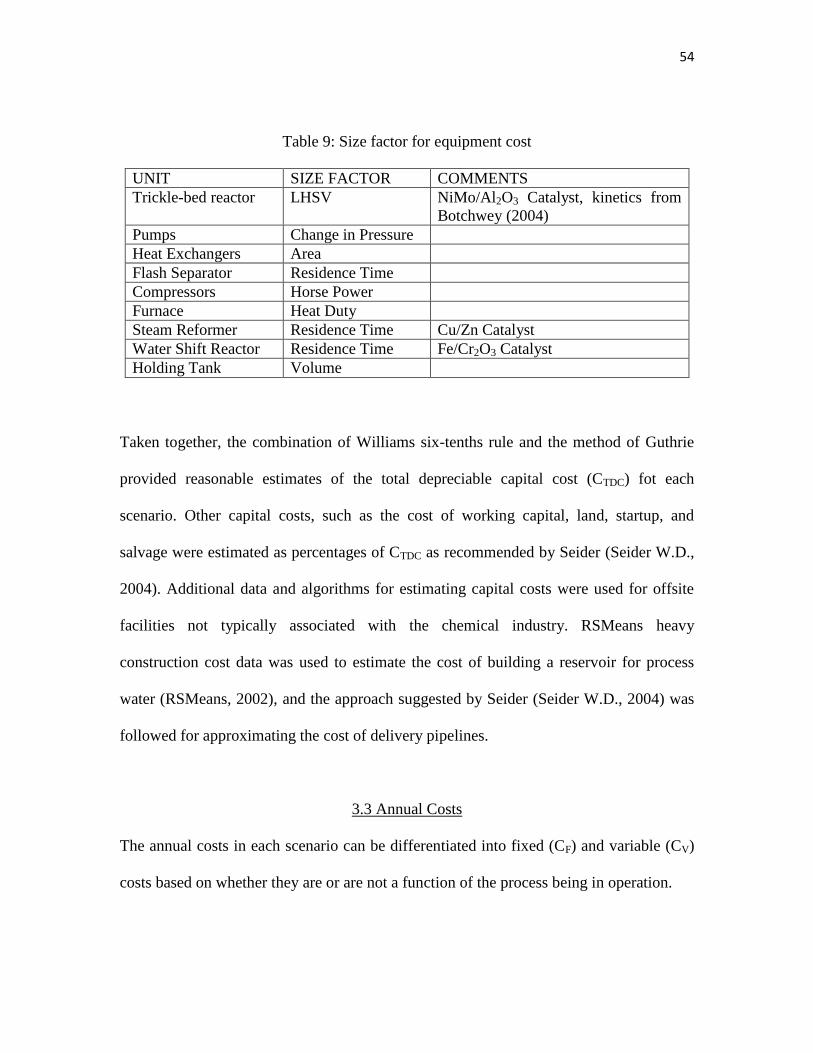
3.1 INTRODUCTION ......................................................................................................... 50
3.2 CAPITAL COSTS ........................................................................................................ 52
3.3 ANNUAL COSTS ........................................................................................................ 54
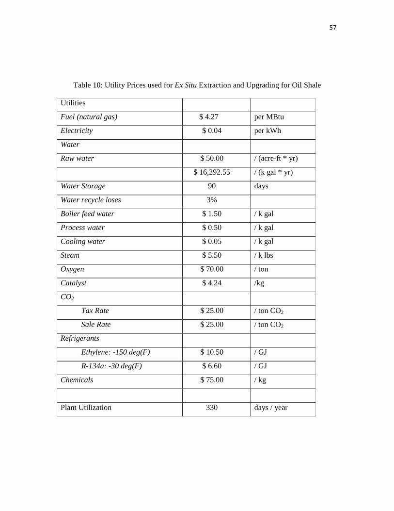
3.3.1 Cost of Utilities to Operate Ex Situ Oil shale Extraction and Upgrading ....... 56
3.4 SALES ....................................................................................................................... 56
3.5 TAXES AND ROYALTIES ............................................................................................ 56
Page 7
vii
OPERATING COST AND ECONOMIC ANALYSIS .................................................... 58
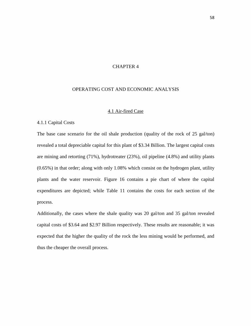
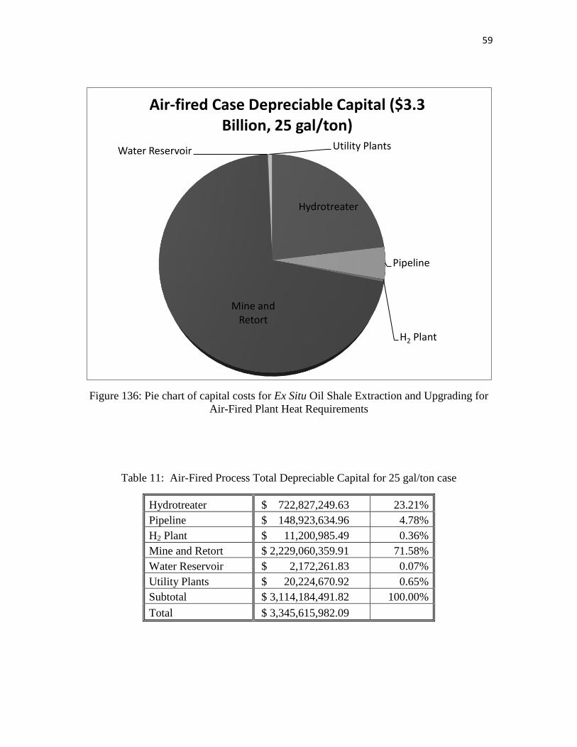
4.1 AIR-FIRED CASE ....................................................................................................... 58
4.1.1 Capital Costs .................................................................................................... 58
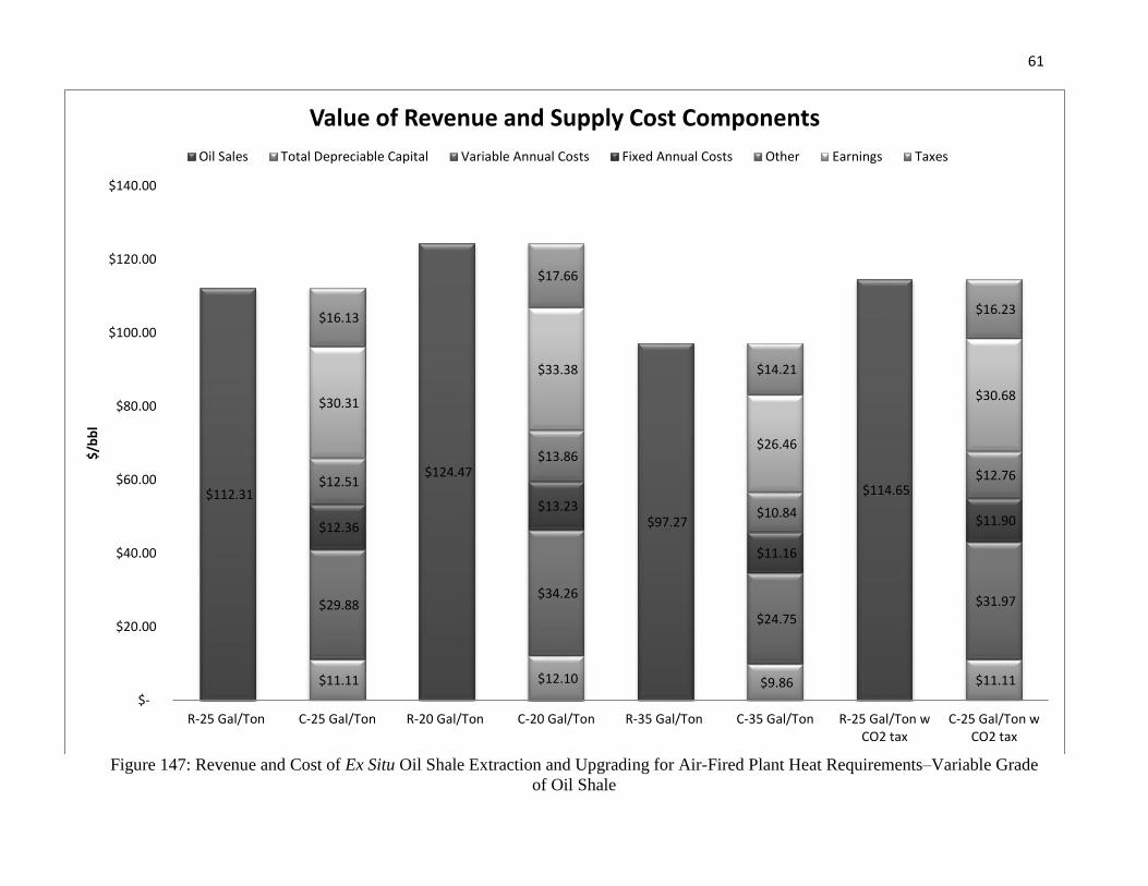
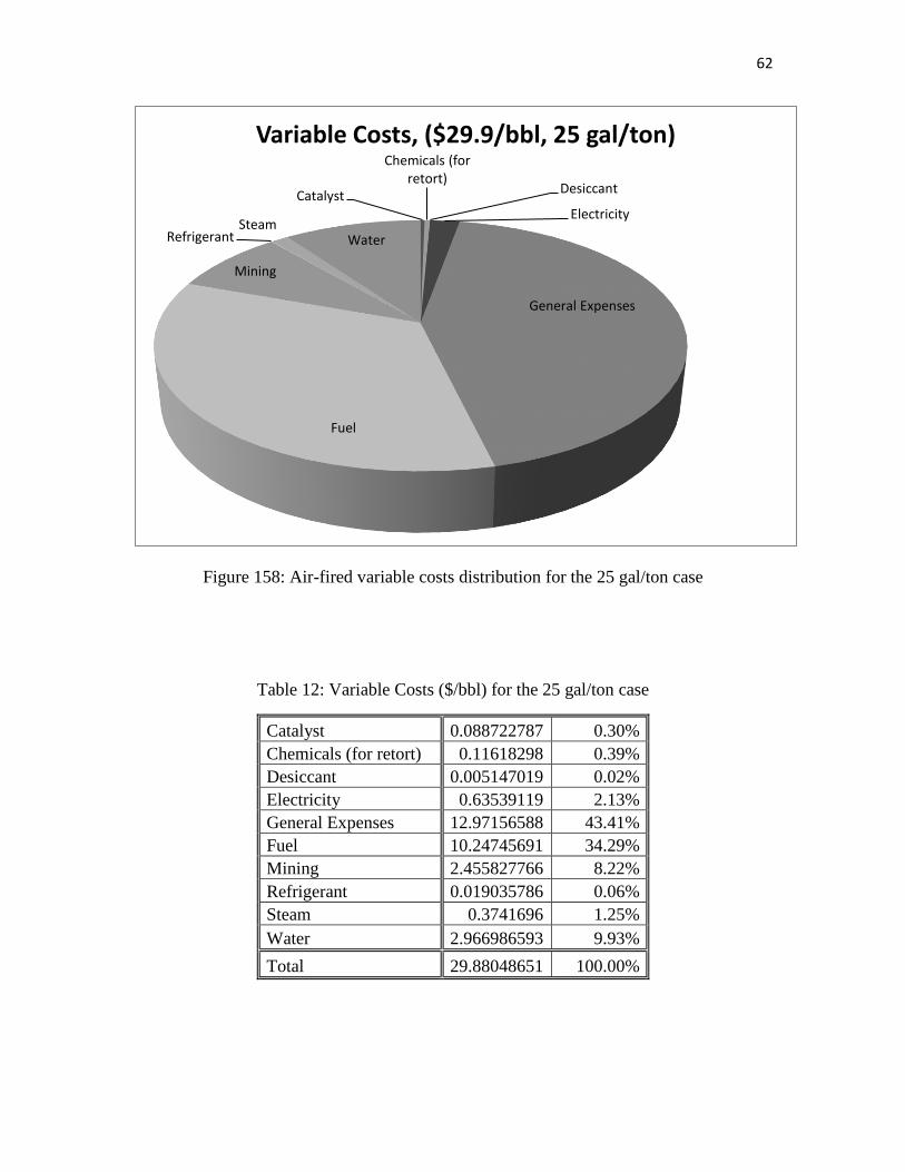
4.1.2 Annual sales and Costs ..................................................................................... 60
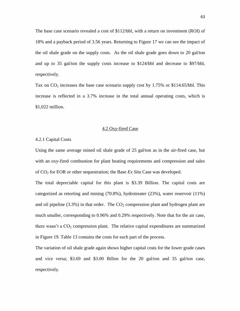
4.2 OXY-FIRED CASE ...................................................................................................... 63
4.2.1 Capital Costs .................................................................................................... 63
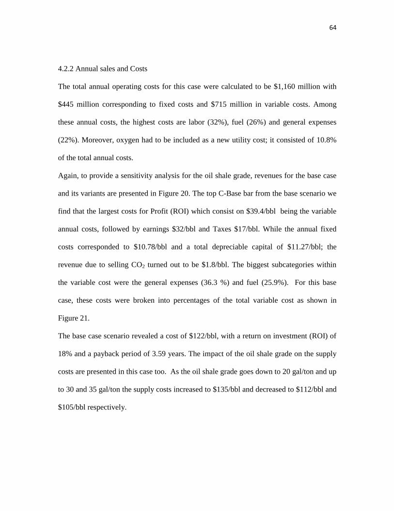
4.2.2 Annual sales and Costs ..................................................................................... 64
4.3 OXY VS AIR-FIRED BURNERS ................................................................................... 68
OTHER IMPORTANT CONSIDERATIONS ................................................................. 69
5.1 SAFETY AND PROCESS CONTROL .............................................................................. 69
5.2 ENVIRONMENTAL ISSUES ......................................................................................... 70
CONCLUSIONS AND RECOMMENDATIONS ........................................................... 71
BIBLIOGRAPHY ............................................................................................................. 73
APPENDICES .................................................................................................................. 76
Page 8
viii
LIST OF TABLES
Table Page
Table 1: Characteristics of Utah Oil Shale (Weiss M.A., 1982) ....................................... 15
Table 2: Design criteria for Pyrolysis, (Weiss M.A., 1982) ............................................. 21
Table 3: Pollution Control ................................................................................................ 22
Table 4: Raw and Upgraded oil characteristics, (Utah Heavy Oil Program INSCC,
University of Utah, 2007) ................................................................................................. 24
Table 5: An economic summary of gasification vs steam reforming for the Natural Gas to
Hydrogen process.............................................................................................................. 40
Table 6: An economic summary for using gasification and steam reforming in parallel,
using the energy generated from gasification to heat the steam reformer. ....................... 40
Table 7: Environmental comparison of steam reforming and shale oil gasification.
Emissions include all gaseous products except CO2......................................................... 42
Table 8: Allocated Capital Investment Costs (Seider W.D., 2004) .................................. 49
Table 9: Size factor for equipment cost ............................................................................ 54
Table 10: Utility Prices used for Ex Situ Extraction and Upgrading for Oil Shale .......... 57
Table 11: Air-Fired Process Total Depreciable Capital for 25 gal/ton case .................... 59
Table 12: Variable Costs ($/bbl) for the 25 gal/ton case .................................................. 62
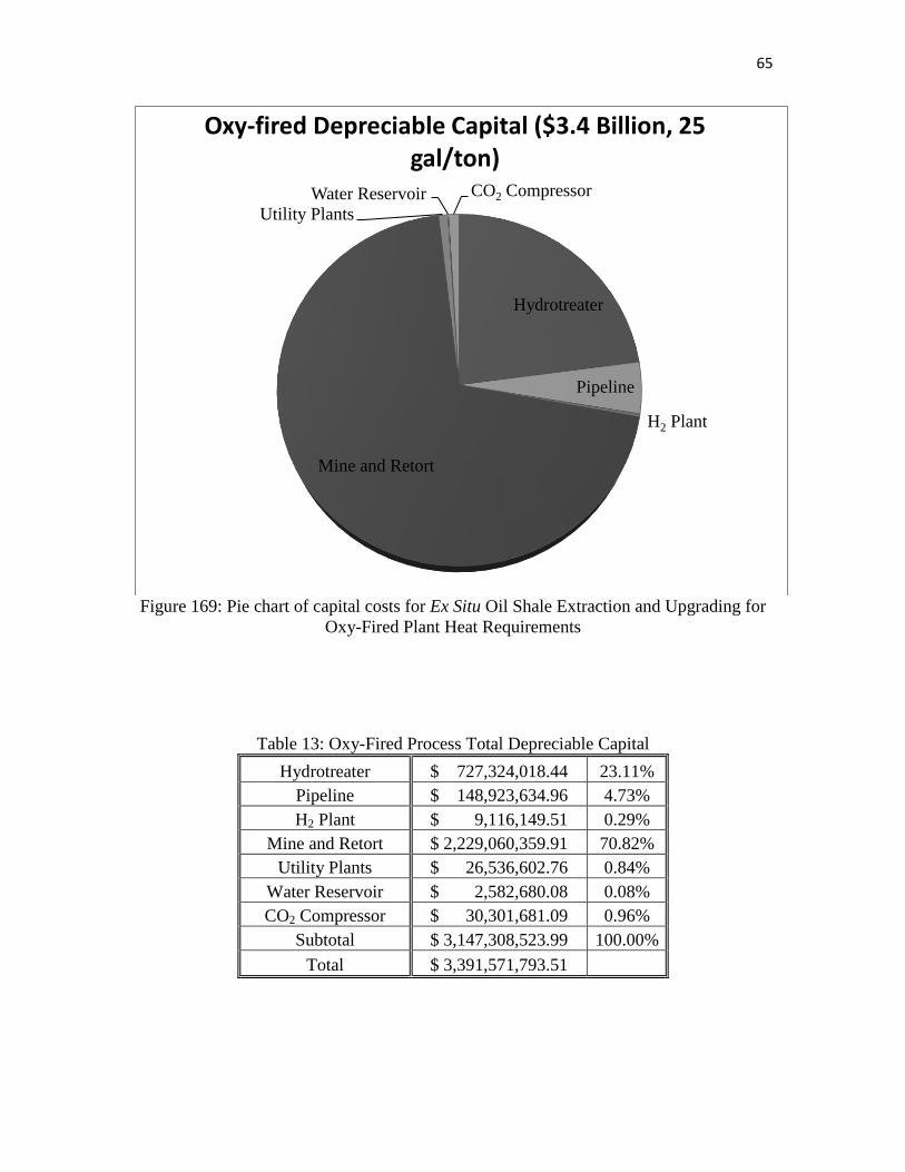
Table 13: Oxy-Fired Process Total Depreciable Capital .................................................. 65
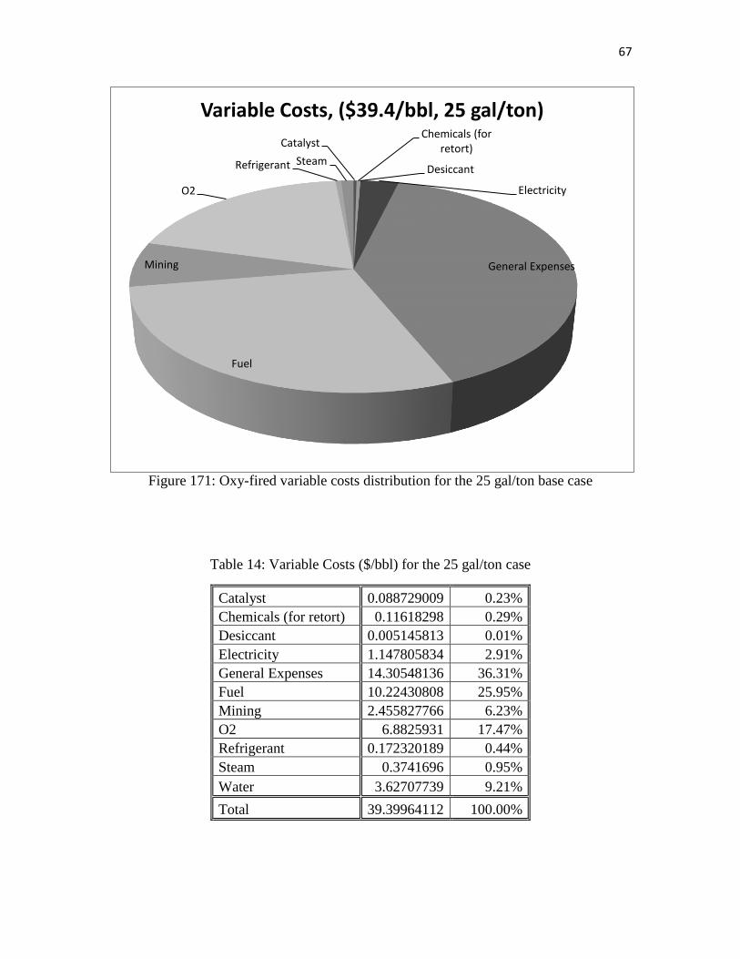
Table 14: Variable Costs ($/bbl) for the 25 gal/ton case .................................................. 67
Page 9
ix
LIST OF FIGURES
Figure Page
Figure 1: Oil Shale Production Methods. ........................................................................... 2
Figure 2: Bonanza and Mine location ............................................................................... 13
Figure 3: Basin-wide Evaluation of the Uppermost Green River Formation's Oil-Shale
Resource, Uinta Basin, Utah and Colorado (VandenBerg, 2008) .................................... 16
Figure 4: Ex Situ Oil Shale Extraction Process Overview using Oxy-fired Combustion . 17
Figure 5: Process Flow Diagram for the Pyrolysis Section (Weiss M.A., 1982) ............. 20
Figure 6: Heavy Oil Upgrading Choices as a function of 343ºC Residue Properties. (Rana
M.S., 2007) ....................................................................................................................... 23
Figure 7 Process Flow Diagram for the Upgrading of Naphtha ....................................... 24
Figure 8: Kinetic model for hydrotreating, (Sanchez S., 2005) ........................................ 26
Figure 9: Hydrogen consumption chart, (Instituto Mexicano del Petroleo, 1979) ........... 29
Figure 10: Block diagram describing the overall natural gas to hydrogen process .......... 32
Figure 11: Using heat transfer fluid to heat the MSR process from the combustion of
methane ............................................................................................................................. 34
Figure 12: Flow rates of each component in the MSR reactor as a function of distance
down the reactor (shown in 10 increments) ...................................................................... 35
Figure 13: Mass flow rates of each component in the Water-Gas shift Reactor as a
function of distance down the reactor (shown in 10 increments) ..................................... 38
Figure 14: Elevation change for pipeline design .............................................................. 45
Figure 15: Process Flow Diagram for CO2 Compression System .................................... 47
Figure 16: Pie chart of capital costs for Ex Situ Oil Shale Extraction and Upgrading for
Air-Fired Plant Heat Requirements .................................................................................. 59
Figure 17: Revenue and Cost of Ex Situ Oil Shale Extraction and Upgrading for Air-Fired
Plant Heat Requirements–Variable Grade of Oil Shale .................................................... 61
Figure 18: Air-fired variable costs distribution for the 25 gal/ton case ............................ 62
Figure 19: Pie chart of capital costs for Ex Situ Oil Shale Extraction and Upgrading for
Oxy-Fired Plant Heat Requirements ................................................................................. 65
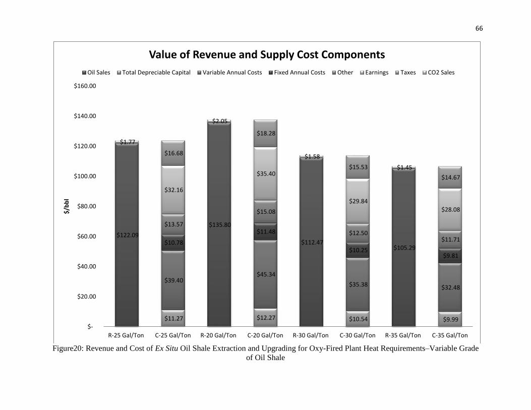
Figure 20: Revenue and Cost of Ex Situ Oil Shale Extraction and Upgrading for Oxy-
Fired Plant Heat Requirements–Variable Grade of Oil Shale .......................................... 66
Figure 21: Oxy-fired variable costs distribution for the 25 gal/ton base case .................. 67
Page 10
x
NOMENCLATURE
Symbol Definition Units
C Costs $
CC Factor determining annual capital charge 1/yr
CF Annual cash flow -
D Pipe diameter in
d Depletion -
E Effectiveness -
F Mass flow rate lb/hr
H Head pump ft
IRR Internal rate of return -
k First order rate constant h-1
K Cost of power $/kWh
L Pipe Length m
LHSV Liquid hourly space velocity h-1
NPV Net present value $
n nth year -
P Production capacity day/yr
PC Cost of pumping power $/kWh
PP Cost of pipe per diameter per length $/in/ft
Q Volumetric flow rate gpm
S Total gross sales $
Sequip Equipment Salvage $
Page 11
xi
T Taxes -
TF Toxicity factor -
W Weight Kg
X Cost of a 2 in schedule 40 carbon steel pipe $/ft
x Mole fraction -
Y Hours of operation per year h/yr
ρ Density kg/m3
μ Viscosity N/m
υ Stoichiometric coefficient
Subscripts
BM Bare-module factor
d Design factor
P Pressure factor
M Material factor
Page 12
1
CHAPTER 1
INTRODUCTION
Our contemporary society depends intensely on oil, since it supplies about 40% of our
total energy demands and more than 99% of the fuel we use for transportation (DOE,
2010). According to the Department of Energy (DOE, 2010), the US and the world may
face a crude oil supply deficit in the future. This oil shortfall could be realistically
overcome by exploiting unconventional sources such as oil shale, heavy oil and tar sands.
In addition, while the US production is expected to decrease, the consumption tends to
increase; intensifying the US oil import dependence. The US Energy Information
Administration released in July 2010 data showing that only five countries exported more
than 1.00 million barrels per day to the United States and noted that this demand is
predicted to increase in the subsequent years (EIA, 2010).
Given that oil shale is one of the alternate sources considered, it is necessary to analyze
its features as a potential solution. First, the total oil shale reserves in America are
estimated to exceed 2 trillion barrels of oil (Bunger J. W., 2004); while about 1.8 trillion
barrels are located in the Green River Formation in western Colorado, southeastern Utah,
and southern Wyoming (Bartis J.T, 2005). Additionally, oil shale richness or areal
density is greater on a per acre basis than other unconventional sources (Bunger J. W.,
2004). The areal density can be translated into technical and economic benefits with
Page 13
2
minimal environmental impacts. These characteristics of the US oil shale resources call
for an intense development to commercialize.
1.1 Overview of current and past oil shale production methods
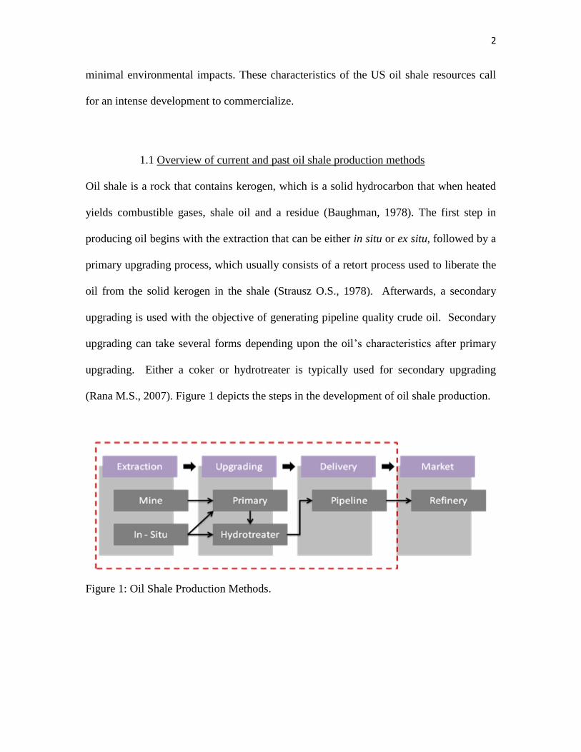
Oil shale is a rock that contains kerogen, which is a solid hydrocarbon that when heated
yields combustible gases, shale oil and a residue (Baughman, 1978). The first step in
producing oil begins with the extraction that can be either in situ or ex situ, followed by a
primary upgrading process, which usually consists of a retort process used to liberate the
oil from the solid kerogen in the shale (Strausz O.S., 1978). Afterwards, a secondary
upgrading is used with the objective of generating pipeline quality crude oil. Secondary
upgrading can take several forms depending upon the oil‟s characteristics after primary
upgrading. Either a coker or hydrotreater is typically used for secondary upgrading
(Rana M.S., 2007). Figure 1 depicts the steps in the development of oil shale production.
Figure 1: Oil Shale Production Methods.
Page 14
3
1.1.1 Extraction and Retort processes
Crude shale oil can be obtained from either in situ (underground) or ex situ
(aboveground) extraction processes. While in an ex situ processing the shale has to be
mined and then surface retorted; in the in situ process, the deposit is fractured and then
retorted underground (Lee, 2000).
a) Ex situ
There are two methods to access the oil shale via mining: room and pillar underground
mining and surface mining. Underground room and pillar mining recovers about 60
percent for layers less than a hundred feet thick; whereas surface mining can be used for
layers over 1,000 feet and multilayered sources if the resource is relatively close to the
surface. Surface mining is subdivided in two types: open pit and strip; open pit can
recover up to 90 percent; but it requires vast areas of terrain (pit~1.5 miles across)
After the extraction process, the oil shale has to be retorted. All surface retorting
processes consist of crushing and sizing the shale, heating it (~900◦F), followed by
cooling and disposal of the spent shale; in addition to, sending the hot shale oil to an
upgrading process.
b) In-situ
During the 1970s and 1980s different in situ processes were investigated, involving
mainly underground burning of the oil shale to produce heat and thus start the retorting
process. However, these methods presented problems in controlling the underground
combustion, which were later resolved by a modified in situ process. This modified in
situ process consisted of mining a portion of the shale which is processed by a surface
retort; the remaining shale is broken uniformly by a series of explosions that ignite and
Page 15
4
burn the underground shale. This modified in-situ process still requires surface action;
therefore, in the early 1980s, researchers considered a new in-situ recovery process. This
new approach consisted of an array of vertical holes; some with a heating element that
would heat the oil shale and others for extraction.
1.1.2 Upgrade, Hydrogen Generation and Delivery
Oil shale crude has a very low pour point temperature and high viscosity making
transportation difficult and expensive. For that reason, in some cases it is more
economical to have partially refined crude before its transportation; the upgrading site is
typically near the retorting site. There are different techniques that can be used to upgrade
oil shale such as visbreaking, coking, catalytic hydrogenation and the addition of
additives.
Visbreaking involves heating the crude to 900◦ to 980
◦F for several minutes. The product
is cooled and the gases that developed during heating are eliminated. This process
efficiently reduces the oil‟s pour point and viscosity; however, there is a modest decrease
in the nitrogen, sulfur and oxygen content. Alternatively, the coking process starts by
heating the oil to the same temperature as visbreaking; proceeded by charging the heated
oil into a vessel, where thermal decomposition occurs. Inside the vessel, the coke is
allowed to fill two-thirds of the drum before the feed is switched into another one.
Catalytic hydrogenation is the most expensive process. It produces the highest quality
products, meaning low nitrogen, sulfur, oxygen and olefinic content. Catalytic
hydrogenation reacts the shale oil with hydrogen in presence of a catalyst. Hydrotreating
opens ring structures and shortens the lengths of the hydrocarbon molecules in the crude
Page 16
5
oil and also plays an important role in removing some of the sulfur as H2S, nitrogen as
ammonia and heavy metals.
Additionally, since hydrogen is needed for the catalytic hydrogenation process, hydrogen
generation is required. A typical hydrogen plant uses natural gas, oxygen, and water as
feeds to produce H2 in three steps. The key step for producing hydrogen comes from the
reaction between methane and water. However this reaction is endothermic and requires a
large amount of heat. The primary source of that heat, which also adds an additional
amount of H2, comes from the partial combustion of natural gas in a gasifier. Finally, CO
in the syn gas from both the steam reformer and gasifier can be combined with water in a
water-gas shift reaction to produce more hydrogen.
1.1.3 Economic Analysis Methods
With the annual production rate and the price of synthetic crude oil established the total
annual sales can be easily determined as the product of these two values. Much of the
effort of this chapter then shifts to the calculation of supply costs. Supply costs are in
two broad categories and consist of capital and operating costs for a given year. Capital
costs are the percentage of the total direct capital costs that are depreciable in a given
year. Operating costs come in two broad categories fixed and variable. They include
land, working capital, utilities, labor, maintenance, taxes and royalties. Many of these
costs are developed based upon the total depreciable capital for the processing plant. The
total depreciable capital is determined by summing up the cost of each piece of
equipment needed for the process as well as any installation expenses.
Page 17
6
1.1.4 Equipment Costing Methods
Supply costs will be developed for the various scenarios using industrial standard
methods for the estimation of capital and operating costs for each year over the life of the
project. Standard accounting methods are used to establish discounted cash flow
predictions for the project allowing various measures of profitability to be established.
Operating costs are determined by accounting for 1) the direct manufacturing costs
including feed stocks, utilities including electricity, water (steam, cooling and process),
refrigeration, fuels, solid waste treatment, waste water treatment and air pollution
abatement as well as labor and maintenance, 2) operating overhead, and 3) fixed costs
including: property taxes and insurance, depreciation, as well as general expenses
including: selling (or transfer) expenses, research (direct or allocated) expenses,
administrative expenses and management incentives. Surface mining costs are estimated
from methods used in civil engineering for large excavations. We will use a mixture of
capital costing methods for this project including:
a) Hill‟s Method (Hill R.D., 1956)
To produce an estimate only two things are needed, a production rate and a flow sheet
showing the major pieces of equipment including: gas compressors, reactors and
separation equipment. Heat exchangers and pumps are not considered in making the
estimate. The estimate uses the Marshall Stevens Process Industry Average Cost Index to
account for inflation in this industry. Different types of processes, e.g. fluid vs. solids
handling, have different cost estimating factors. Additional factors to account for site
preparation, services facilities, utility plants and related facilities can be added. The
Page 18
7
estimate is accurate to approximately ±50% and is particularly useful for low-pressure
petrochemical plants.
b) Lang‟s Method (Peters M.S., 1968)
This method requires a process design, complete with a mass and energy balance and
equipment sizing. The estimate uses overall factors that multiply estimates of the
delivered cost of all the process equipment including: heat exchangers, pumps, gas
compressors, reactors and separation equipment. Important factors account for the effects
on unit cost of construction materials, operating pressure and delivery costs of the
equipment. The estimate uses the Marshall Stevens Process Industry Average Cost Index
to account for inflation in this industry. Different types of processes, e.g. fluid vs. solids
handling, have different cost estimating factors. Using various Lang factors either the
total permanent investment (fixed capital investment) or the total capital investment
(including working capital at 17.6% of total permanent investment) can be determined.
The estimate is accurate to approximately ±35%.
c) Guthrie‟s Method (Guthrie K.M., 1974)
The method requires an optimal process design with mass and energy balance, equipment
sizing, selection of construction materials and a process control configuration. To apply
the Guthrie method f.o.b purchase cost of each piece of equipment is estimated as is the
case with the Lang method. Instead of using an overall factor to account for equipment
installation and other capital costs, individual factors for each type of equipment are used.
This allows the construction materials to be different for a reactor or separation unit and
the platforms and ladders required to access it for example. To the summation of installed
equipment costs, the components of total permanent investment including; contingency
Page 19
8
and contractor fees, site development costs, building costs and offsite facility costs, are
added. The total permanent investment cost is added to the working capital to determine
the total capital investment. The estimate uses the Chemical Engineering Cost Index to
account for inflation by equipment type in this industry. The estimate is accurate to
approximately ±20%.
A similar ex situ oil shale case was done in the 1980‟s by Weiss at MIT‟s Energy
Laboratory. We cannot improve on that processing route but will modify it to a new site
and today‟s standards. The capital costs have been updated for a new production rate and
a 2010 purchase date using Hill‟s method and the operating costs have been updated to
modern unit operation costs. In all other cases, the capital costs have been estimated by
the Guthrie method where possible or the Lang method where not. The annualized costs
of the capital investment are determined over the life of the plant giving annualized
capital expenses which are added to the annual operating costs for the plant to determine
the annual cost for producing the annual production of the plant. The annual cost divided
by the annual production rate of the plant gives the supply cost for that year. Making
assumptions about the sales price for the crude oil to the refinery and its price sensitivity,
the pre-tax profit from the production and upgrading operations developed for this
scenario will be determined as well as the depreciation, depletion and income taxes for
these operations. Finally, various rigorous profitability measures such as annual cash
flow, annual net present value and investor‟s rate of return will be determined.
Page 20
9
1.2. Obstacles to development
Oil shale development is constrained by various factors such as the economics and the
environmental impact involved in its production.
An oil shale facility can be very costly, meaning expensive oil. Although the price of oil
shale is expected to be competitive now and in the future; it is still a risky investment.
This investment consists not only of the mining, retorting and upgrading design and
development aspects; but also, requires a supporting infrastructure such as roads,
pipelines, power lines, waste treatment and pollution control facilities. According to a
government supported operation in Colorado, it was required an investment of $1.2
billion (2005 dollars) and a production cost of approximately $ 100 per barrel (2005
dollars).
Waste disposal is one limitation to oil shale development. Retorting produces large
quantities of waste rock which undergoes a ten percent volume increase during the
process; these rocks generate a disposal problem (Yen T.F., 1979). Allain (Allain, 1980)
reported that 1012
Btu of oil produced, generates over 350,000 tons of spent shale. On
addition, the spent shale still contains significant quantities of oil which requires
treatment before disposal. Air pollution also has to be considered as another constraint.
The production of oil generates major pollutants such as CO, NOX SO2, as well as
particulates generated from crushing and blasting oil shale rocks (Allain, 1980). Another
environmental limitation is dictated by the oil shale‟s location which has a limited water
supply since its sources are mainly concentrated in semi-arid areas. Water consumption
and water disposal are major problems. These issues create the necessity for a new
contingent infrastructure that has to be considered such as reservoirs, solid waste
Page 21
10
treatment plants and pipelines. Moreover, the surface area required for mining and
retorting can create land damage which influences natural flora and fauna, as well as the
natural aesthetic beauty of the landscape (Allain, 1980).
Although the afore mentioned issues affect oil shale development, the central economic
problem is the fact that it is only about 10-15% of the mass is recoverable as marketable
energy and the remaining 85-90% incurs a considerable expense just to process and
dispose of it in an environmentally acceptable manner. By contrast with conventional
fossil fuels, essentially 70-90% of recovered product ((e.g. 70-90% of coal, up to 100%
(ex water and sulfur) of natural gas and 100% (ex water) of oil)) consist of usable
energy, i.e., burnable. Conversely, large volumes of shale must be mined, handled,
processed, and disposed of in order to recover a relatively small amount of shale oil by
traditional methods of surface retorting; all of that is expensive.
In some locations, a second key problem exists: heavy burdens imposed by the
particular location – Utah‟s Uinta Basin. The terrain is difficult, making construction
expensive. Water supplies are limited; their use for energy purposes has provoked
serious social and institutional debate for over 30 years. Population is sparse; the
infrastructure does not exist to provide and support the people needed to build and
operate an oil shale industry. Environmental restrictions may limit the size of the
industry or require more extensive (and expensive) emission controls for air, water and
solid wastes.
One technical approach to the lean-ore problem is in situ extraction. By leaving all or
most of the rock in the ground and processing it there, materials handling problems are
significantly reduced. Several methods of in situ recovery have been proposed and
Page 22
11
researched. Although technical feasibility has been demonstrated oil can be produced-
economic feasibility has not been demonstrated to date and the future for in situ recovery
is not clear.
1.3. Goal of the project
The purpose of this project is to examine the limiting factors to oil shale development and
determine the commercial viability with a supply cost analysis. To complete this study,
an engineering cost estimate was performed, an assessment of market conditions under
which processes breaks even as well as a sensitivity of processes to price volatility and
resource quality.
Page 23
12
CHAPTER 2
PROCESS DESCRIPTION
2.1. Scenario specifications
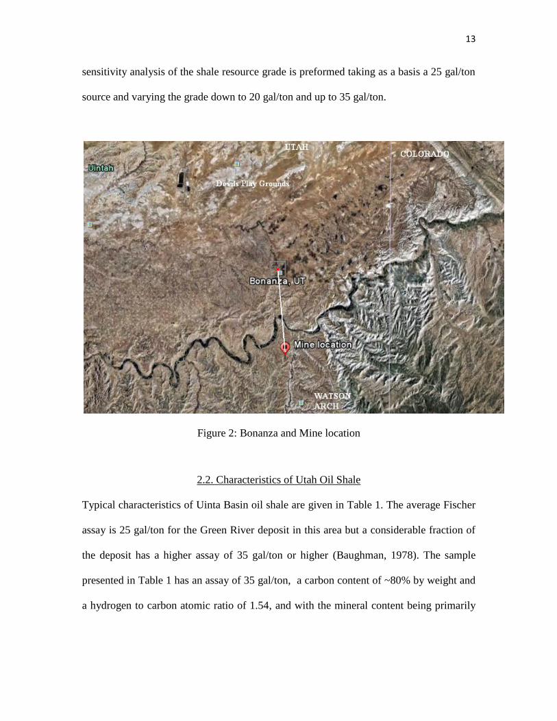
This project studied oil shale production at a scale of 50,000 barrels a day. The location
of this resource is the OSEC property near Bonanza, UT, as shown in Figure 2. This
resource is estimated to have a quality ranging from 25 to 35 gallons per ton of oil shale
(Baughman, 1978).
The technology used assumed a room-and-pillar mining process with one-bench and a
60ft thick seam at a depth ranging from 600 to 860 feet and a TOSCO II retort. The
hydrotreater was specified to be a trickle- bed reactor with a commercial NiMo/Al2O3
catalyst; while the hydrogen plant was based on a steam reformer/gas shift reaction. The
pipeline is assumed to run in a straight line from the mine location to Vernal and then to
North Salt Lake, UT., with an approximate distance of 379.6 km.
The oil shale scenario was divided in two cases, one assuming oxy-fired combustion with
a CO2 sequestration process. This process mainly consisted of a compression/cooling
process to produce a pipeline quality CO2 product. The other case assumed a regular air-
fired burner with stack emissions.
In the air case, air was assumed to be 20% oxygen, 79% nitrogen and 1% argon on a
mole basis; while in the oxy-fired case assumed to be pure oxygen. In each case a
Page 24
13
sensitivity analysis of the shale resource grade is preformed taking as a basis a 25 gal/ton
source and varying the grade down to 20 gal/ton and up to 35 gal/ton.
Figure 2: Bonanza and Mine location
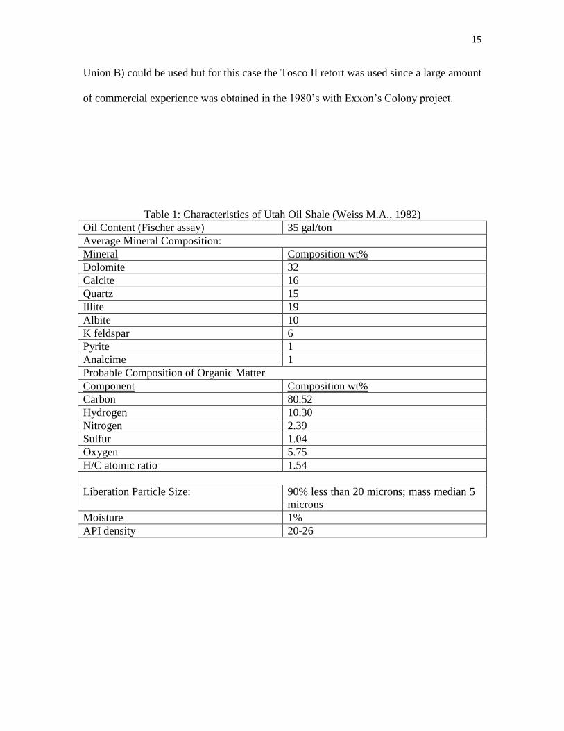
2.2. Characteristics of Utah Oil Shale
Typical characteristics of Uinta Basin oil shale are given in Table 1. The average Fischer
assay is 25 gal/ton for the Green River deposit in this area but a considerable fraction of
the deposit has a higher assay of 35 gal/ton or higher (Baughman, 1978). The sample
presented in Table 1 has an assay of 35 gal/ton, a carbon content of ~80% by weight and
a hydrogen to carbon atomic ratio of 1.54, and with the mineral content being primarily
Page 25
14
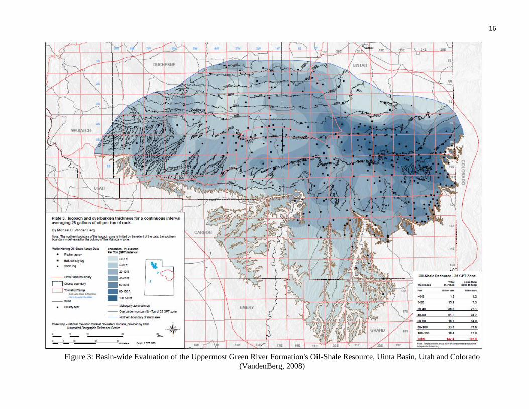
carbonate minerals, dolomite and calcite. Figure 3 shows an isopach and overburden
thickness for a continuous interval averaging 25 gal/ton.
2.3. Process Overview
In this scenario, we will focus on ex situ extraction involving mining and surface retort
technologies to extract the oil from the oil shale. The location of this resource is the
OSEC property near Bonanza, UT as shown in Figure 2. The Mohagany zone varies
considerably in this area but is approximately 1,000 ft deep suggesting that underground
mining is possible. Ore beneficiation using fine grinding and froth flotation before
retorting was studied by (Weiss M.A., 1982) and was not found to be an economic
improvement over direct retorting. This was due to the high capital and energy costs for
grinding for the flotation step as well as the added uncertainty of the process. Grinding
technology has not significantly improved since the time of the Weiss report so ore
beneficiation has not been considered in this assessment (Weiss M.A., 1982).
Supercritical extraction may also be used for beneficiation but this technology is even
more highly uncertain than that of froth flotation. However, it may play a role in in situ
methods.
Underground mining for Oil shale starts between 500 and 2,000 ft down in an
underground mine. The oil shale is blasted from the mine‟s wall and transported to the
surface where a comminution circuit grinds it down to less than 0.5 in. and it is placed in
covered storage. The ground shale is moved by belt conveyor to the retort. Any one of a
number of retort technologies (Tosco II, Lurgi, Paraho direct (licensed to Petrobras),
Page 26
15
Union B) could be used but for this case the Tosco II retort was used since a large amount
of commercial experience was obtained in the 1980‟s with Exxon‟s Colony project.
Table 1: Characteristics of Utah Oil Shale (Weiss M.A., 1982)
Oil Content (Fischer assay) 35 gal/ton
Average Mineral Composition:
Mineral Composition wt%
Dolomite 32
Calcite 16
Quartz 15
Illite 19
Albite 10
K feldspar 6
Pyrite 1
Analcime 1
Probable Composition of Organic Matter
Component Composition wt%
Carbon 80.52
Hydrogen 10.30
Nitrogen 2.39
Sulfur 1.04
Oxygen 5.75
H/C atomic ratio 1.54
Liberation Particle Size: 90% less than 20 microns; mass median 5
microns
Moisture 1%
API density 20-26
Page 27
16
Figure 3: Basin-wide Evaluation of the Uppermost Green River Formation's Oil-Shale Resource, Uinta Basin, Utah and Colorado
(VandenBerg, 2008)
Page 28
17
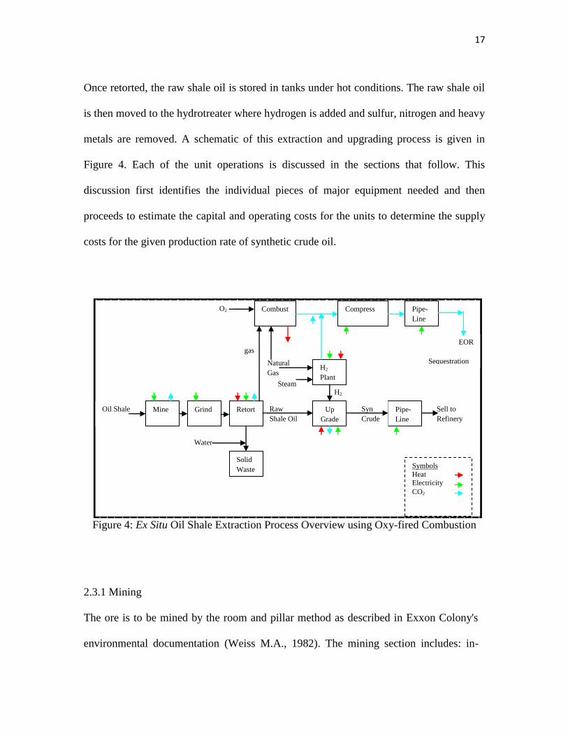
Once retorted, the raw shale oil is stored in tanks under hot conditions. The raw shale oil
is then moved to the hydrotreater where hydrogen is added and sulfur, nitrogen and heavy
metals are removed. A schematic of this extraction and upgrading process is given in
Figure 4. Each of the unit operations is discussed in the sections that follow. This
discussion first identifies the individual pieces of major equipment needed and then
proceeds to estimate the capital and operating costs for the units to determine the supply
costs for the given production rate of synthetic crude oil.
2.3.1 Mining
The ore is to be mined by the room and pillar method as described in Exxon Colony's
environmental documentation (Weiss M.A., 1982). The mining section includes: in-
O2
gas
Natural
Gas
H2
Oil Shale
Deposit
Mine Grind
H2
Plant
Solid
Waste
Raw
Shale Oil
Up
Grade
Pipe-
Line
Syn
Crude
Retort
Water
Sell to
Refinery
Steam
Symbols
Heat Electricity
CO2
Combust Compress Pipe-
Line
EOR
Sequestration
Figure 4: Ex Situ Oil Shale Extraction Process Overview using Oxy-fired Combustion
Page 29
18
mine haulage, primary cone crushing, the required surface truck fleet and coarse shale
storage. The quantity of rock that must be mined each day at 25 gal/ton oil shale grade
is 85,512 ton/day to yield 50,000 bbl/day.
2.3.2 Comminution and Solids Handling
Oil shale particles are separated by density since kerogen density averages about 1.07
while the density of the minerals averages 2.7 (Weiss M.A., 1982). To perform this
separation, it is necessary to crush and blast oil shale rocks followed by comminution.
The additional comminution includes secondary crushing (to 0.5 inch), covered storage
of crushed shale, a linking belt conveyor system from the grinding units to the storage
system. Impact crushers are used for secondary crushing.
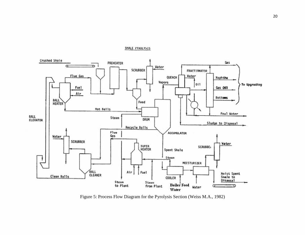
2.3.3 Pyrolysis
The process design of the pyrolysis section was based chiefly on the environmental
documentation from the Exxon Colony Project (Weiss M.A., 1982). The flow sheet is
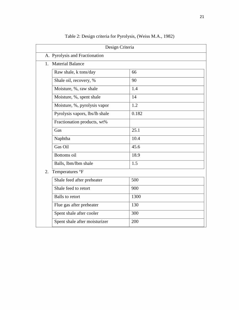
shown in Figure 5. The plant has six parallel trains. The design criteria are listed in
Table 2. The raw shale from the second stage crusher is preheated with flue gases from
the ball heater and fed into the retort together with steam and hot ceramic balls that act
as a heat transfer medium. The retort includes a rotating inclined drum in which the
shale and balls are intimately mixed before they pass into the accumulator. Overhead
vapors include hydrocarbons, carbon monoxide and dioxide, ammonia, hydrogen
sulfide, water, and hydrogen. They are quenched with cooling water and separated into
gas, naphtha, gas oil, bottoms oil, and foul water in a fractionator. The naphtha
Page 30
19
separation together with processing of the other streams is part of the upgrading section.
The spent shale is separated from the balls in a rotating trommel screen at the bottom of
the accumulator and is discharged through a cooler (waste heat recover) boiler to a
moisturizer.
The moist spent shale is then taken by conveyor to the waste disposal area. The balls are
recycled to the retort drum via a cleaner and heater. In the cleaner, dust is removed from
the balls using the flue gases from a steam super heater. Steam facilities are not fully
shown in Figure 5 because they are integrated with the steam generator for the entire
plant. The spent shale contains all the original raw shale with a few percent of
unrecoverable kerogen or its non-volatile organic derivatives. The waste effluents and
corresponding pollution control equipment are summarized in Table 3. The data are
based on the environmental documentation from Weiss. (Weiss M.A., 1982)
Dust from the conveyor belts is a relatively small pollution source. Gas and liquid
effluents from the pyrolysis step originate primarily from the kerogen. Dust effluents
from the pyrolysis originate primarily from the oil shale.
Page 31
20
Figure 5: Process Flow Diagram for the Pyrolysis Section (Weiss M.A., 1982)
Page 32
21
Table 2: Design criteria for Pyrolysis, (Weiss M.A., 1982)
Design Criteria
A. Pyrolysis and Fractionation
1. Material Balance
Raw shale, k tons/day 66
Shale oil, recovery, % 90
Moisture, %, raw shale 1.4
Moisture, %, spent shale 14
Moisture, %, pyrolysis vapor 1.2
Pyrolysis vapors, lbs/lb shale 0.182
Fractionation products, wt%
Gas 25.1
Naphtha 10.4
Gas Oil 45.6
Bottoms oil 18.9
Balls, lbm/lbm shale 1.5
2. Temperatures °F
Shale feed after preheater 500
Shale feed to retort 900
Balls to retort 1300
Flue gas after preheater 130
Spent shale after cooler 300
Spent shale after moisturizer 200
Page 33
22
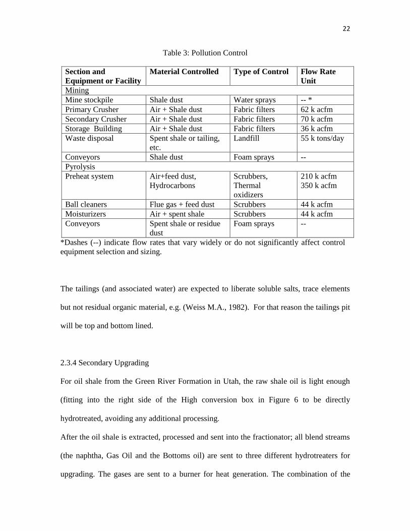
Table 3: Pollution Control
Section and
Equipment or Facility
Material Controlled Type of Control Flow Rate
Unit
Mining
Mine stockpile Shale dust Water sprays -- *
Primary Crusher Air + Shale dust Fabric filters 62 k acfm
Secondary Crusher Air + Shale dust Fabric filters 70 k acfm
Storage Building Air + Shale dust Fabric filters 36 k acfm
Waste disposal Spent shale or tailing,
etc.
Landfill 55 k tons/day
Conveyors Shale dust Foam sprays --
Pyrolysis
Preheat system Air+feed dust,
Hydrocarbons
Scrubbers,
Thermal
oxidizers
210 k acfm
350 k acfm
Ball cleaners Flue gas + feed dust Scrubbers 44 k acfm
Moisturizers Air + spent shale Scrubbers 44 k acfm
Conveyors Spent shale or residue
dust
Foam sprays --
*Dashes (--) indicate flow rates that vary widely or do not significantly affect control
equipment selection and sizing.
The tailings (and associated water) are expected to liberate soluble salts, trace elements
but not residual organic material, e.g. (Weiss M.A., 1982). For that reason the tailings pit
will be top and bottom lined.
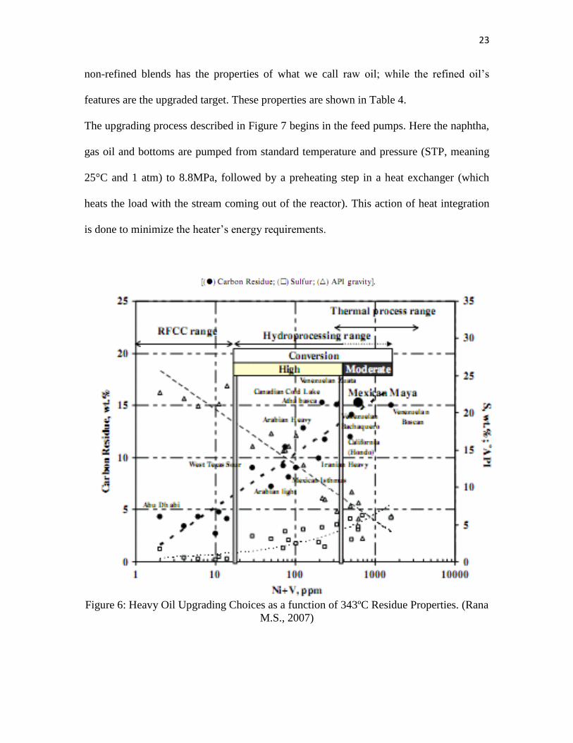
2.3.4 Secondary Upgrading
For oil shale from the Green River Formation in Utah, the raw shale oil is light enough
(fitting into the right side of the High conversion box in Figure 6 to be directly
hydrotreated, avoiding any additional processing.
After the oil shale is extracted, processed and sent into the fractionator; all blend streams
(the naphtha, Gas Oil and the Bottoms oil) are sent to three different hydrotreaters for
upgrading. The gases are sent to a burner for heat generation. The combination of the
Page 34
23
non-refined blends has the properties of what we call raw oil; while the refined oil‟s
features are the upgraded target. These properties are shown in Table 4.
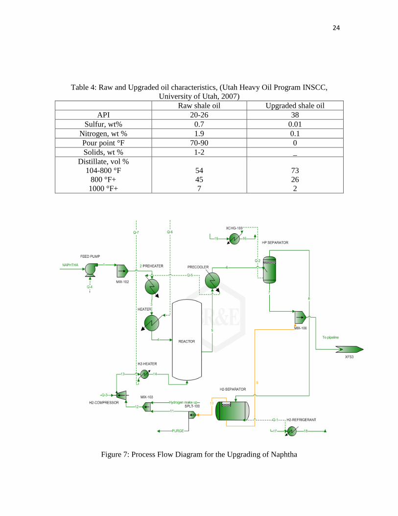
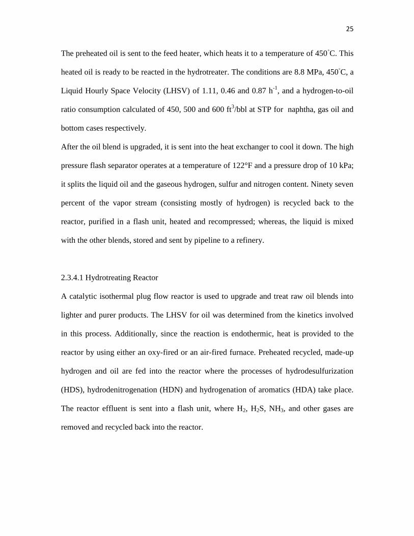
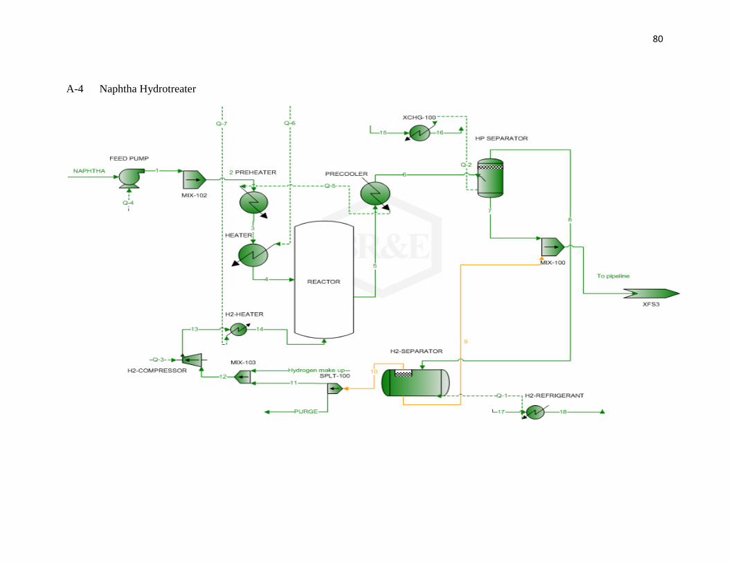
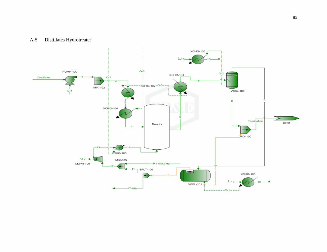
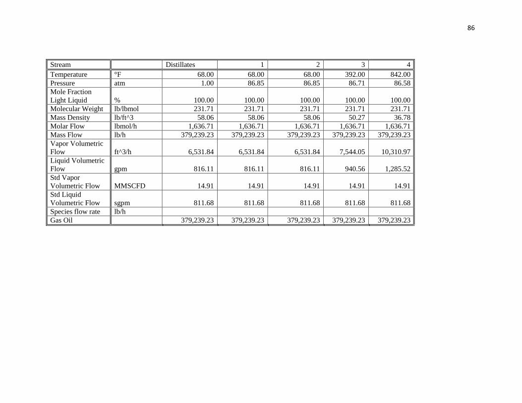
The upgrading process described in Figure 7 begins in the feed pumps. Here the naphtha,
gas oil and bottoms are pumped from standard temperature and pressure (STP, meaning
25°C and 1 atm) to 8.8MPa, followed by a preheating step in a heat exchanger (which
heats the load with the stream coming out of the reactor). This action of heat integration
is done to minimize the heater‟s energy requirements.
Figure 6: Heavy Oil Upgrading Choices as a function of 343ºC Residue Properties. (Rana
M.S., 2007)
Page 35
24
Table 4: Raw and Upgraded oil characteristics, (Utah Heavy Oil Program INSCC,
University of Utah, 2007)
Raw shale oil Upgraded shale oil
API 20-26 38
Sulfur, wt% 0.7 0.01
Nitrogen, wt % 1.9 0.1
Pour point °F 70-90 0
Solids, wt % 1-2 _
Distillate, vol %
104-800 °F
800 °F+
1000 °F+
54
45
7
73
26
2
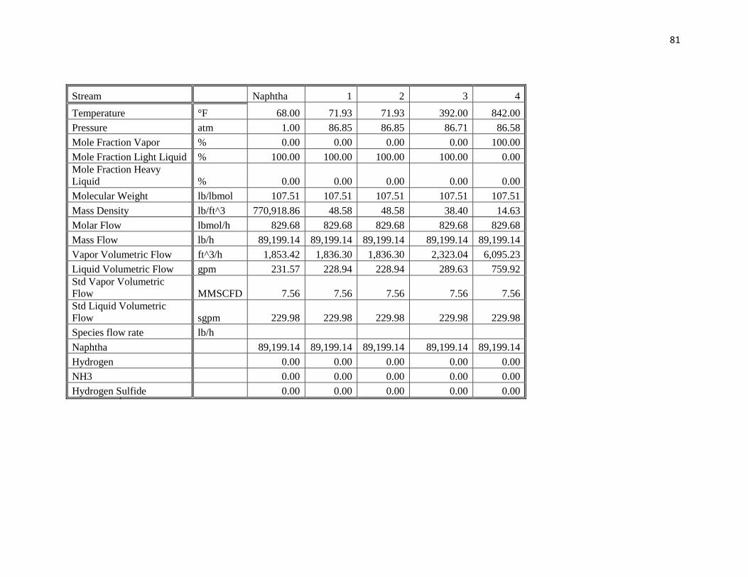
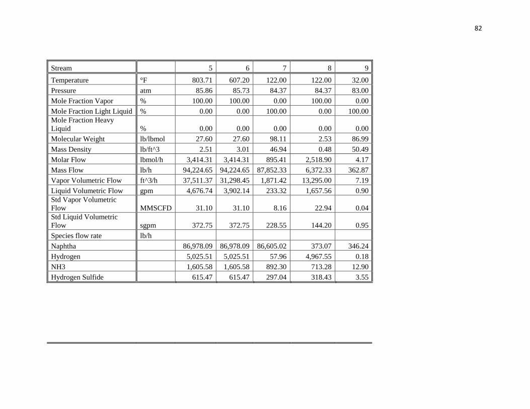
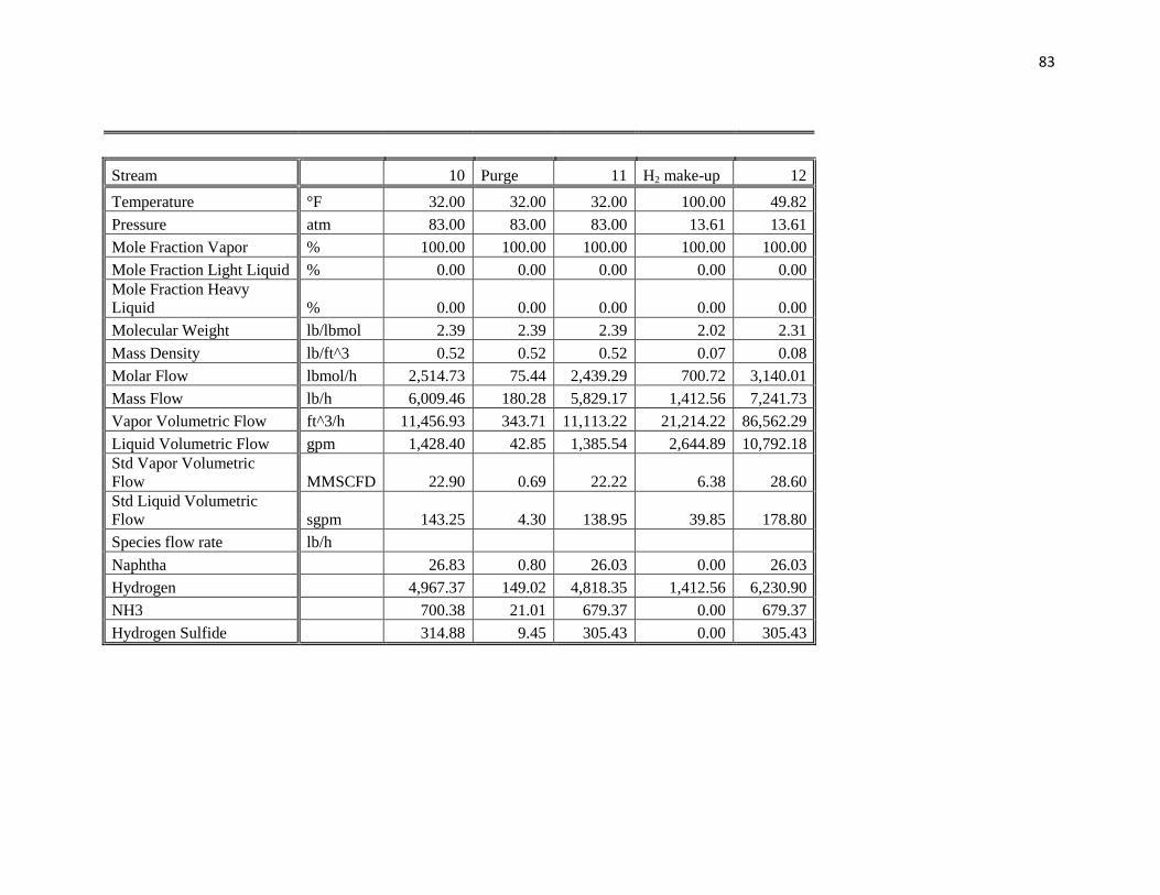
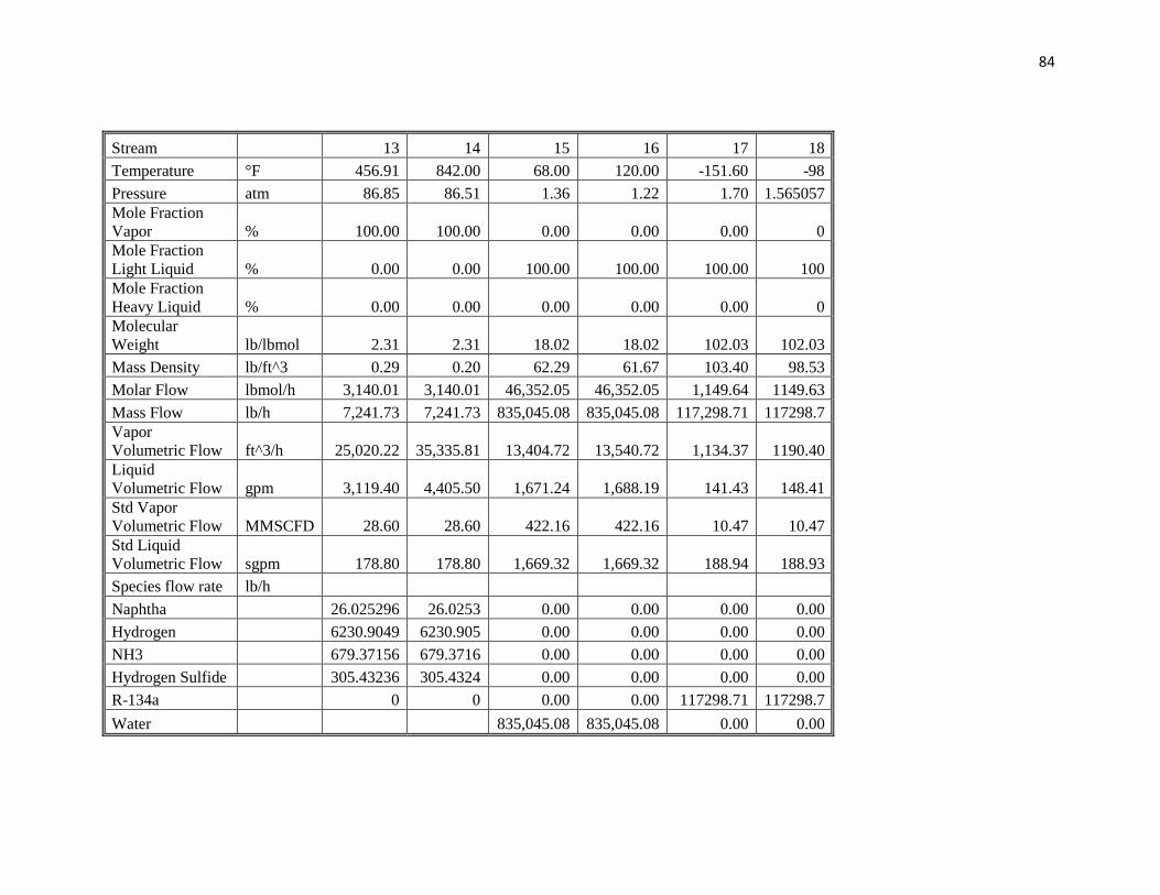
Figure 7: Process Flow Diagram for the Upgrading of Naphtha
Page 36
25
The preheated oil is sent to the feed heater, which heats it to a temperature of 450◦C. This
heated oil is ready to be reacted in the hydrotreater. The conditions are 8.8 MPa, 450◦C, a
Liquid Hourly Space Velocity (LHSV) of 1.11, 0.46 and 0.87 h-1
, and a hydrogen-to-oil
ratio consumption calculated of 450, 500 and 600 ft3/bbl at STP for naphtha, gas oil and
bottom cases respectively.
After the oil blend is upgraded, it is sent into the heat exchanger to cool it down. The high
pressure flash separator operates at a temperature of 122°F and a pressure drop of 10 kPa;
it splits the liquid oil and the gaseous hydrogen, sulfur and nitrogen content. Ninety seven
percent of the vapor stream (consisting mostly of hydrogen) is recycled back to the
reactor, purified in a flash unit, heated and recompressed; whereas, the liquid is mixed
with the other blends, stored and sent by pipeline to a refinery.
2.3.4.1 Hydrotreating Reactor
A catalytic isothermal plug flow reactor is used to upgrade and treat raw oil blends into
lighter and purer products. The LHSV for oil was determined from the kinetics involved
in this process. Additionally, since the reaction is endothermic, heat is provided to the
reactor by using either an oxy-fired or an air-fired furnace. Preheated recycled, made-up
hydrogen and oil are fed into the reactor where the processes of hydrodesulfurization
(HDS), hydrodenitrogenation (HDN) and hydrogenation of aromatics (HDA) take place.
The reactor effluent is sent into a flash unit, where H2, H2S, NH3, and other gases are
removed and recycled back into the reactor.
Page 37
26
2.3.4.2 Catalytic reactor kinetics
Determining every single reaction that occurs during the hydrotreatment process is not
reasonable. For that reason, a general chemical reaction is used to summarize the main
aspects of the process. According to Owusu; this reaction can be written as (Owusu,
2005):
→
[1]
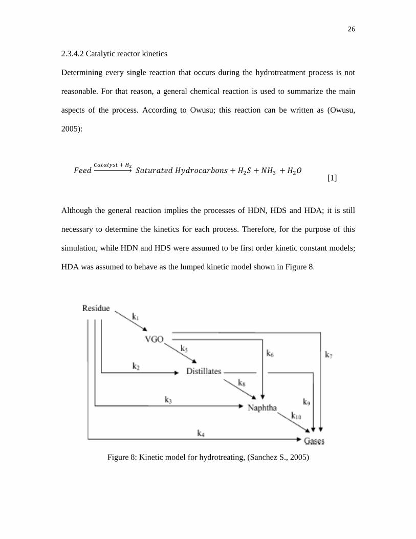
Although the general reaction implies the processes of HDN, HDS and HDA; it is still
necessary to determine the kinetics for each process. Therefore, for the purpose of this
simulation, while HDN and HDS were assumed to be first order kinetic constant models;
HDA was assumed to behave as the lumped kinetic model shown in Figure 8.
Figure 8: Kinetic model for hydrotreating, (Sanchez S., 2005)
Page 38
27
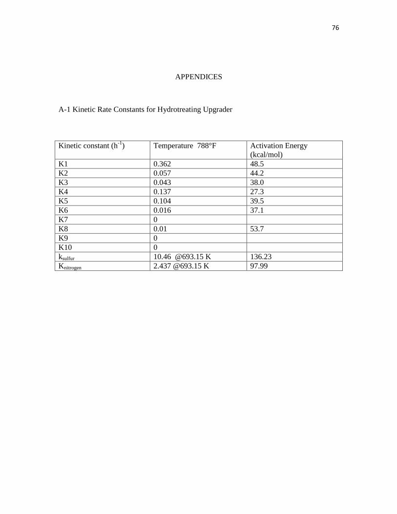
All of the kinetic constants and activation energies are shown in Appendix A-1 and are
computed within the simulation for specific operating conditions. Since the kinetic
model was used to determine the LHSV (which is required to determine the size of the
reactor) that would achieve the desired conversion; conversion was defined as:
[
] [2]
where EP indicates the fraction of the substance in the feed or product boiling point
above the desired endpoint. These boiling endpoints were classified as unconverted
residues (1000.4 °F +), vacuum gas oil (VGO; 649.4-1000.4 °F), distillates (399.2-649.4
°F), naphtha (Initial Boiling Point (IBP)-399.2 °F) and gases.
The desired conversion was determined as the target characteristics of the oil that will be
sent through the pipeline. After getting different LHSV values for each boiling endpoint,
HDN and HDS; the smallest LHSV was chosen to be the operational condition for the
reactor. The rationale for this is that the smallest LHSV implies the reaction limiting step
or the reaction that takes the longest to occur.
To compute the volume of the reactor, it was necessary to consider the residence time of
oil inside the reactor, the volume of hydrogen present at operational conditions and the
catalyst volume.
The volume of the catalyst required in the reactor is a function of the oil volumetric flow
and the LHSV chosen:
Page 39
28
Vcatalyst = Volumetric Flow Rate of Oil/LHSV
[3]
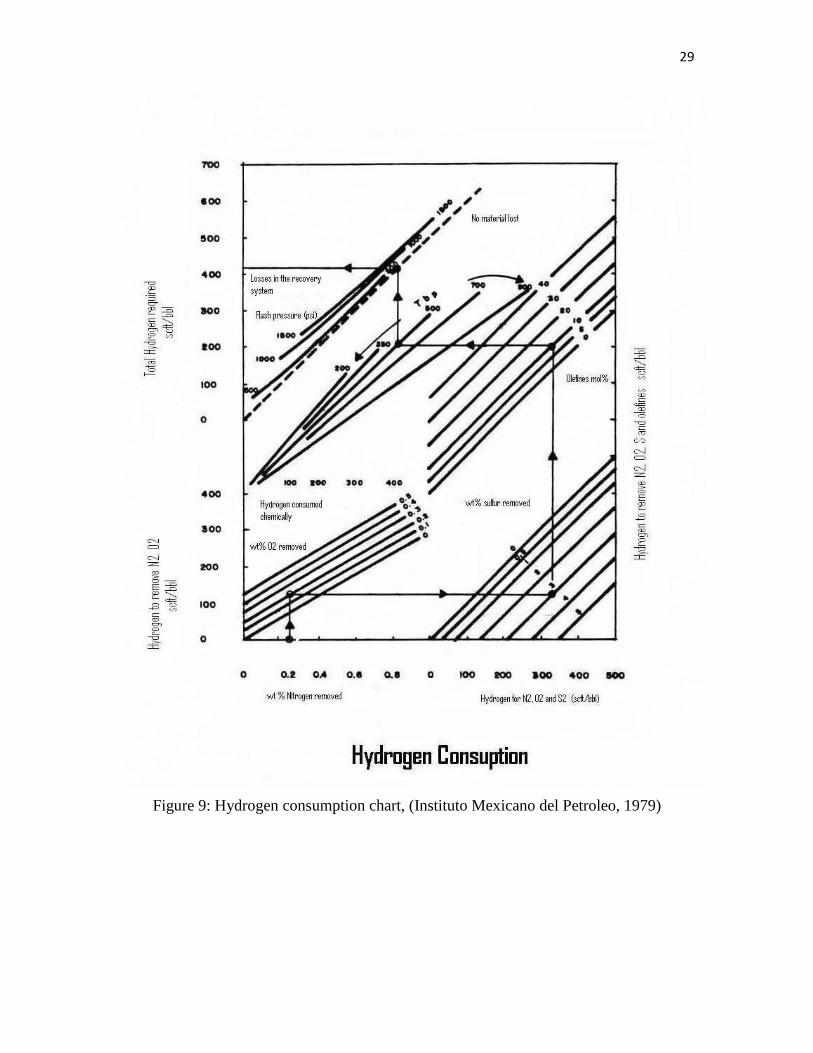
The hydrogen consumption was calculated using the graphical method that is shown in
Figure 9 and was used as follows. Considering the composition of an oil blend to
upgrade, with a sulfur removal of 0.69 wt%, a nitrogen removal of 1.8 wt% and an olefin
crack of 38.61wt% and a flash operating at a pressure over 1200 psi; the total hydrogen
consumption was estimated to be of 500 scft/bbl of oil.
Finally, an additional 10% was added to the reactor volume for an overdesign
contingency.
2.3.4.3 Energy and Mass Balances
To keep the reactor isothermal, an energy balance was required, considering the enthalpy
flow rate in and out of the reactor, as well as the heat consumed per pound of material
reacted ~220 Btu/lb (Wilson J.W., 1997), and the hydrogen heating requirement. A
burner was simulated to produce the heat requirement for the reactor and the feed heater.
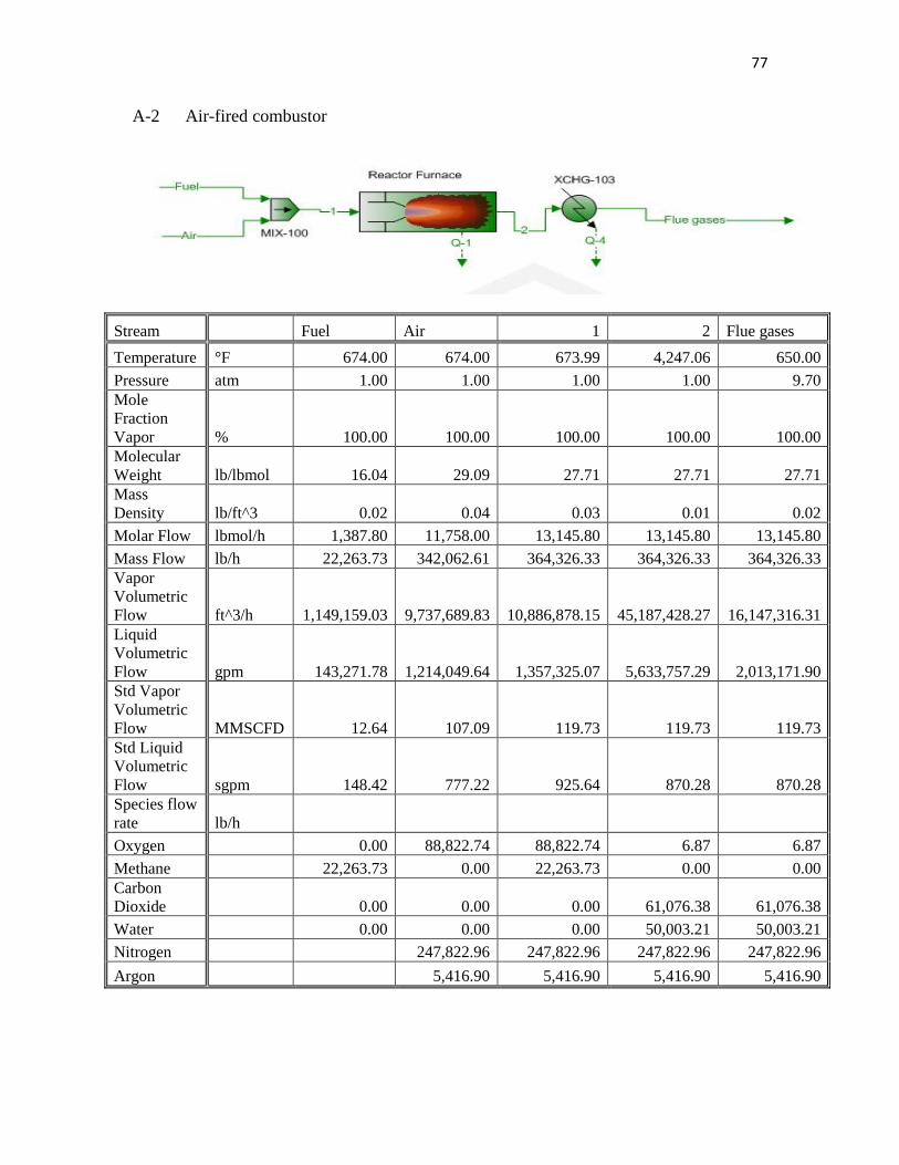
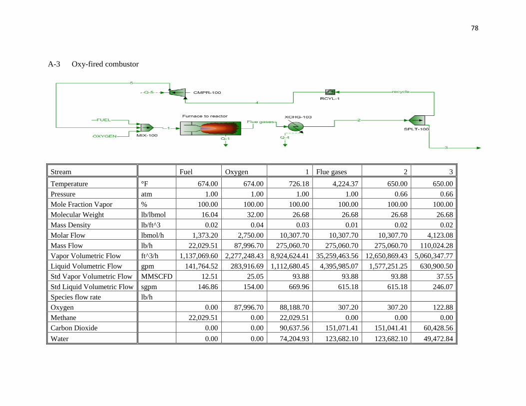
2.3.4.4 Burner configurations
The air and oxy-fired burners used in this project have different configurations. The oxy-
fired burner has a CO2 recycle loop and recompression stage to compensate for any
pressure drops. The purpose of this configuration is to lower the temperature of the
burner to the adiabatic flame temperature of the regular air-fired burner. The process flow
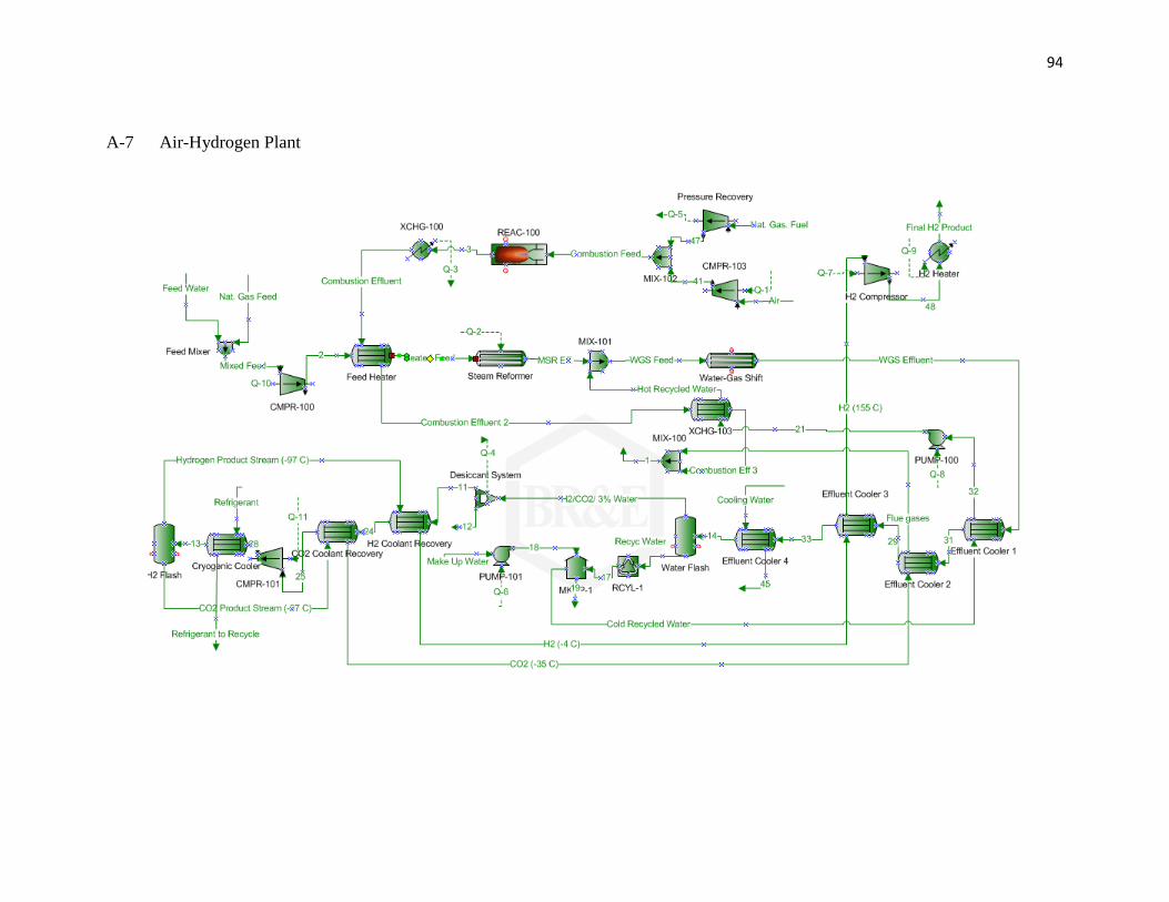
diagrams for both furnaces are depicted in Appendix A-2 and A-3.
Page 40
29
Figure 9: Hydrogen consumption chart, (Instituto Mexicano del Petroleo, 1979)
Page 41
30
These reactors are specified to react stoichiometrically with an inlet temperature of 674°F
and atmospheric pressure. The efficiency of the reactor is dictated by the flue gases
temperature which was specified as 650°F, (Seider W.D., 2004). The reason for this
temperature is to avoid condensation of the flue gases and consequent corrosion.
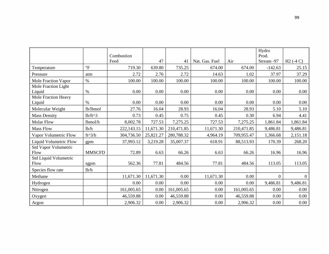
2.3.5 Hydrogen Plant
In order to upgrade the shale oil to the point where it can be pumped in a traditional
pipeline hydrogen has to be added to the crude. Assuming that the shale oil is produced
from a commercial scale operation located in the Green River Basin; an estimated of 1.94
kg of H2 /bbl must be added to the oil.
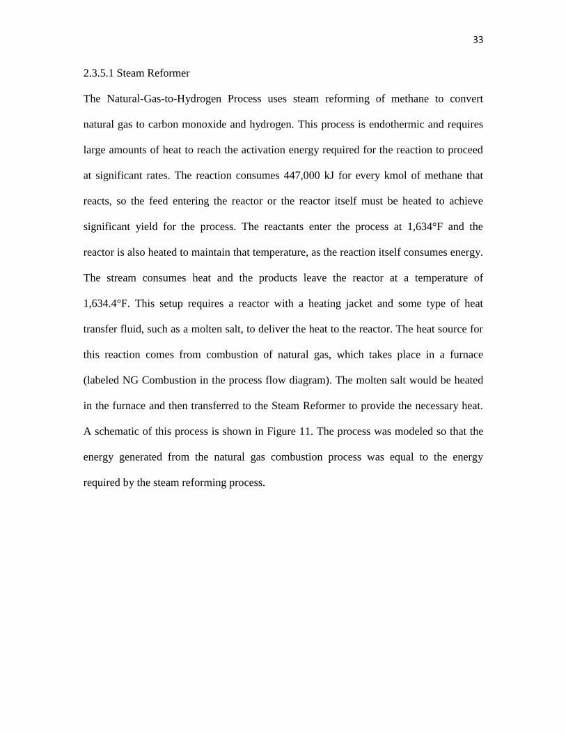
The hydrogen plant utilizes a natural gas boiler, methane steam reformer, water-gas shift
reactor, and two flash tanks for H2 separation. See Figure 10 for a process schematic. The
process uses natural gas, oxygen, and water as feeds to produce H2 in three steps. The key
step for producing hydrogen is given in Equation 4:
[4]
However this reaction is endothermic and requires a large amount of heat. The primary
source of that heat (and of an additional amount of H2) comes from the partial
combustion of natural gas in a gasifier:
[5]
Page 42
31
Finally, CO in the syn gas from both the steam reformer and gasifier can be combined
with water in a water-gas shift reaction:
[6]
Water-gas shift reactions are typically carried out in two stages with a high (350oC) and a
low (200oC) temperature step. However, in our design, we found that acceptable levels of
CO conversion were achieved without the low temperature step.
Environmental concerns include the formation of hazardous pollutants such as NOX,
SOX, particulate matter, H2S, and CO. However, perhaps the biggest environmental
concern is the amount of water that this process could consume.
Water usage is negligible compared to the average flow of the Green River (the nearest
major water source), which is approximately 3,950 Mgal/day (Enright M., 2005), if oil
shale development accelerates in the Green River Formation, water usage could become a
serious issue.
Steam reforming of methane is used to convert natural gas to hydrogen and carbon
monoxide. This process takes place at 1634 °F and 600 psia. Steam is fed in excess to the
process to push the equilibrium in favor of hydrogen and carbon monoxide. 97.7% of the
methane is converted in this process. The heat for this reaction is generated from
combustion of natural gas in another reactor. The effluent from the steam reformer is
combined with additional steam and fed to a water gas shift reactor, which takes
advantage of the carbon monoxide in the stream by oxidizing it and reducing water to
Page 43
32
form more hydrogen. The water gas shift takes place at 590 °F and 590 psia and results in
conversion of 94% of the carbon monoxide to form additional hydrogen.
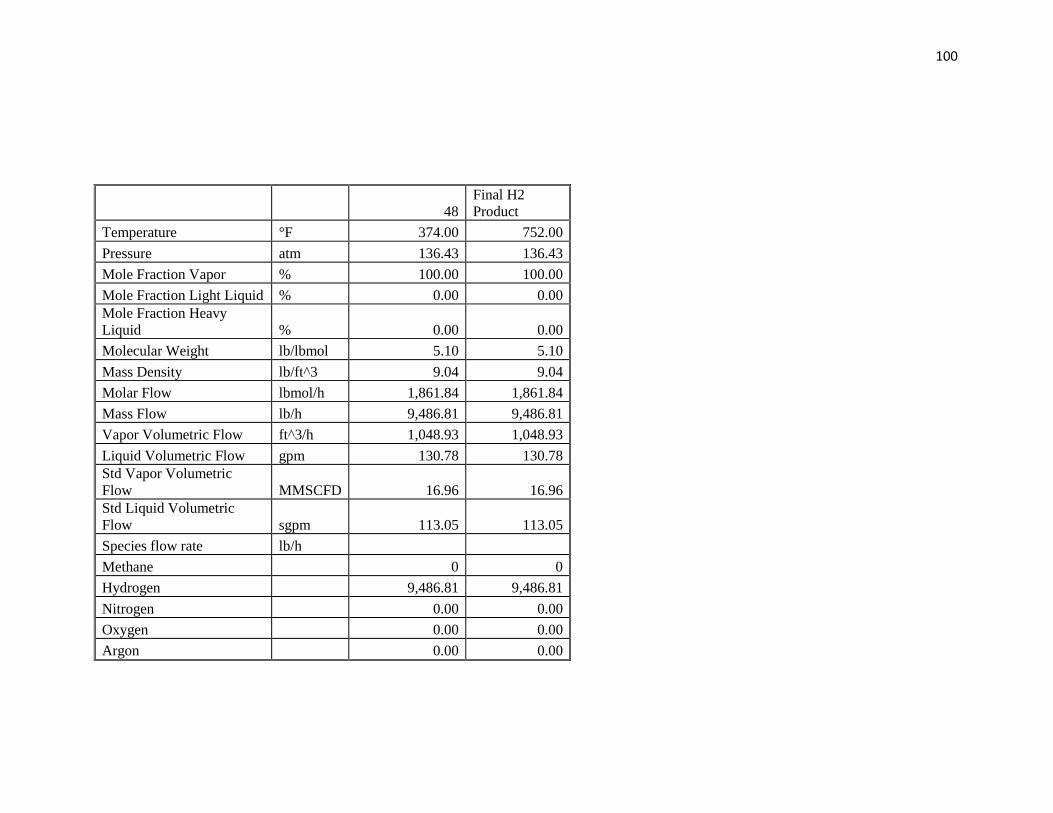
The effluent from the reaction sequence is then cooled to 176 °F, where most of the water
is removed by a flash tank. This water is 99.8 % pure and can be recycled back to the
water gas shift process, which requires excess steam so that the equilibrium favors the
hydrogen product. The carbon dioxide and hydrogen are then separated by a high
pressure and low temperature flash, which results in a stream that is 90.3 % pure
hydrogen. Although this process requires large amounts of refrigeration to reach the very
low temperatures required to condense carbon dioxide, this was deemed to be the most
economical CO2 removal technique because it does not require large solvent flow rates or
the equipment necessary for an absorption/stripping process.
Steam
Reforming of
Methane at 1634
°F and 600 psia
Water Gas Shift
at 590°F and 590 psia
Natural Gas
Combustion at
40 psia
Natural Gas:
65079 lb/h
Steam:
79434 lb/h
Water Separation
(Flash at 176 °F
and 540 psia)
Water
Recycle
Hydrogen Carbon
Dioxide
Separation (Flash
at -125 °F and 2030 psia)
Natural Gas:
43258 lb/h
Air: 718726
lb/h
Combustion
Effluent Gases
Heat Delivered
to Reformer
Hydrogen Product
90.3% pure (molar)
82312 lb/h
Carbon Dioxide Product
96.4% pure (molar)
101405 lb/h
Figure 10: Block diagram describing the overall natural gas to hydrogen process.
Page 44
33
2.3.5.1 Steam Reformer
The Natural-Gas-to-Hydrogen Process uses steam reforming of methane to convert
natural gas to carbon monoxide and hydrogen. This process is endothermic and requires
large amounts of heat to reach the activation energy required for the reaction to proceed
at significant rates. The reaction consumes 447,000 kJ for every kmol of methane that
reacts, so the feed entering the reactor or the reactor itself must be heated to achieve
significant yield for the process. The reactants enter the process at 1,634°F and the
reactor is also heated to maintain that temperature, as the reaction itself consumes energy.
The stream consumes heat and the products leave the reactor at a temperature of
1,634.4°F. This setup requires a reactor with a heating jacket and some type of heat
transfer fluid, such as a molten salt, to deliver the heat to the reactor. The heat source for
this reaction comes from combustion of natural gas, which takes place in a furnace
(labeled NG Combustion in the process flow diagram). The molten salt would be heated
in the furnace and then transferred to the Steam Reformer to provide the necessary heat.
A schematic of this process is shown in Figure 11. The process was modeled so that the
energy generated from the natural gas combustion process was equal to the energy
required by the steam reforming process.
Page 45
34
Combustion Furnace
Methane Steam Reformer
HotCold
12
3 4
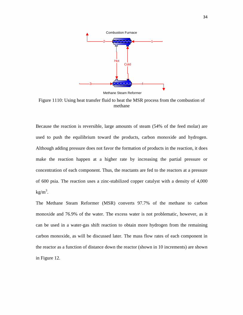
Figure 1110: Using heat transfer fluid to heat the MSR process from the combustion of
methane
Because the reaction is reversible, large amounts of steam (54% of the feed molar) are
used to push the equilibrium toward the products, carbon monoxide and hydrogen.
Although adding pressure does not favor the formation of products in the reaction, it does
make the reaction happen at a higher rate by increasing the partial pressure or
concentration of each component. Thus, the reactants are fed to the reactors at a pressure
of 600 psia. The reaction uses a zinc-stabilized copper catalyst with a density of 4,000
kg/m3.
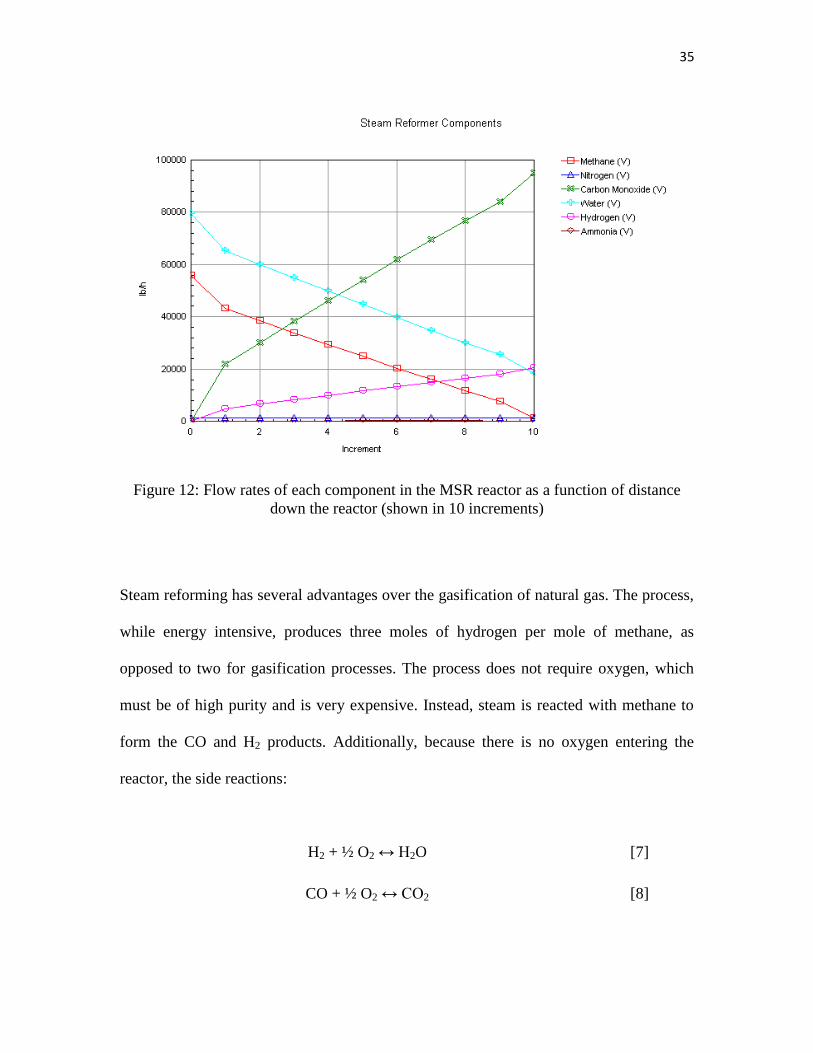
The Methane Steam Reformer (MSR) converts 97.7% of the methane to carbon
monoxide and 76.9% of the water. The excess water is not problematic, however, as it
can be used in a water-gas shift reaction to obtain more hydrogen from the remaining
carbon monoxide, as will be discussed later. The mass flow rates of each component in
the reactor as a function of distance down the reactor (shown in 10 increments) are shown
in Figure 12.
Page 46
35
Figure 12: Flow rates of each component in the MSR reactor as a function of distance
down the reactor (shown in 10 increments)
Steam reforming has several advantages over the gasification of natural gas. The process,
while energy intensive, produces three moles of hydrogen per mole of methane, as
opposed to two for gasification processes. The process does not require oxygen, which
must be of high purity and is very expensive. Instead, steam is reacted with methane to
form the CO and H2 products. Additionally, because there is no oxygen entering the
reactor, the side reactions:
H2 + ½ O2 ↔ H2O [7]
CO + ½ O2 ↔ CO2 [8]
Page 47
36
do not consume the desired products, and greater yield of H2 and CO can be achieved.
The process does have disadvantages compared to gasification, however. The steam
reforming process does nothing with the heavier hydrocarbons in the natural gas. Also,
gasification is highly exothermic and does not require utilities to heat the streams. In fact,
the energy from the gasifcation reaction can be used to heat other streams or generate
steam for electricity generation.
2.3.5.2 Ammonia Formation
Another reaction added to the reaction set for the steam reformer was the formation of
ammonia from hydrogen and nitrogen.
3H2 + N2 ↔ 2NH3 [9]
In order to quantify the formation of ammonia, this reaction was added to the reaction set
for the steam reformer. It was assumed that the reaction is governed by equilibrium.
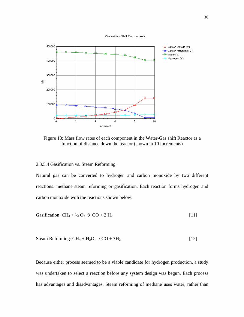
2.3.5.3 Water-Gas Shift Reactor
The water-gas shift reaction can be used to form additional hydrogen from carbon
monoxide by the reaction:
CO + H2O ↔ CO2 + H2 [10]
Page 48
37
Reactants enter the reactor at 590°F and exit at 781.6°F since the reaction is exothermic.
The inlet pressure is 590 psia and the reactor has a 10 psia pressure drop. Additional
water is added to the feed stream to push the reaction further toward the formation of
carbon dioxide and hydrogen. The reactor uses an iron oxide catalyst that is promoted
with chromium oxide with a density of 1300 kg/m3. The mass balance for this reactor is
shown in Figure 13.
The reactor has a conversion of 94% based on carbon monoxide, which is the limiting
reactant. Because of this high rate of conversion, another water-gas shift reactor is not
used. It proves to be very difficult to get additional conversion from the carbon monoxide
as the large amounts of hydrogen and carbon dioxide already in the stream push the
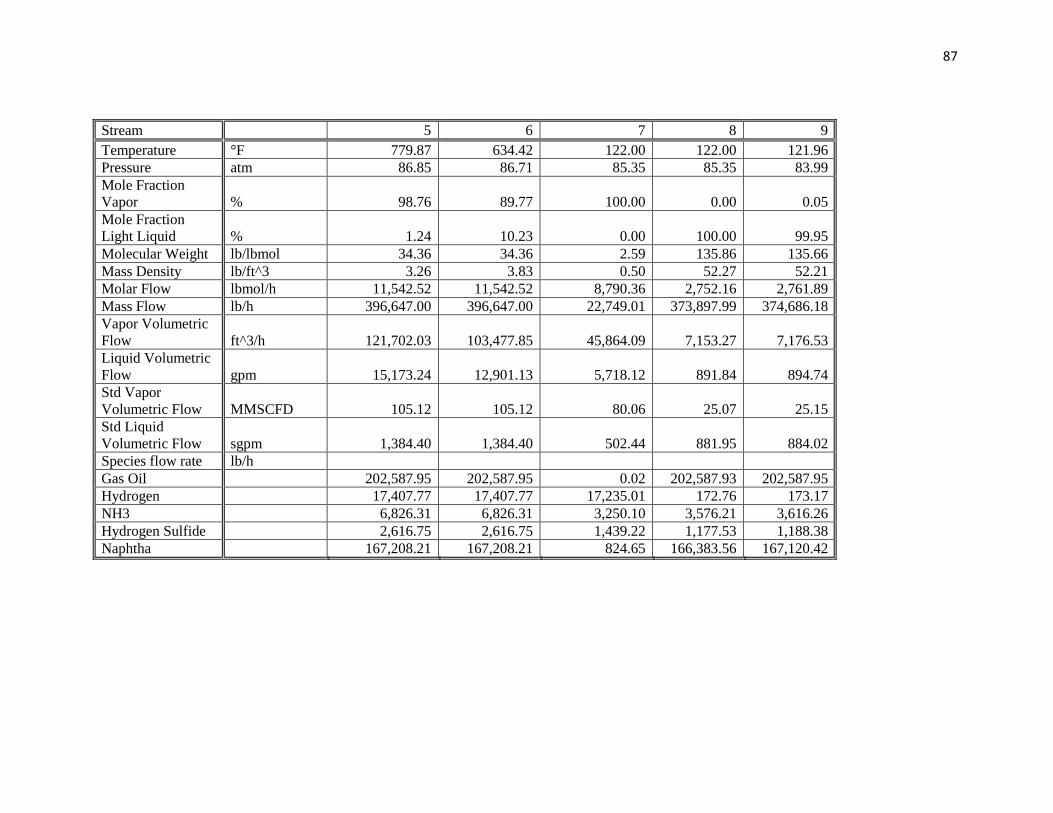
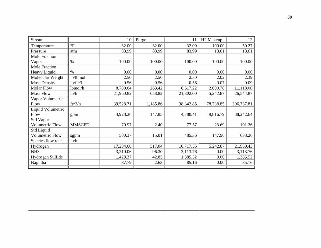
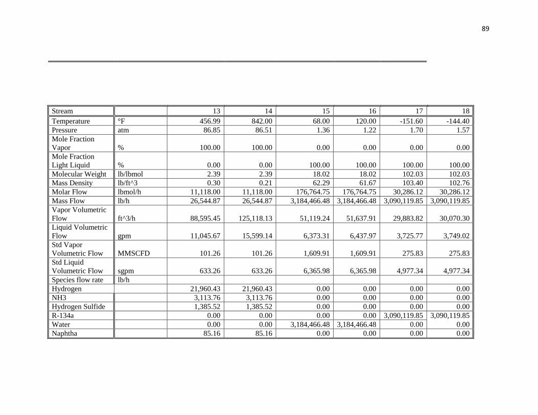
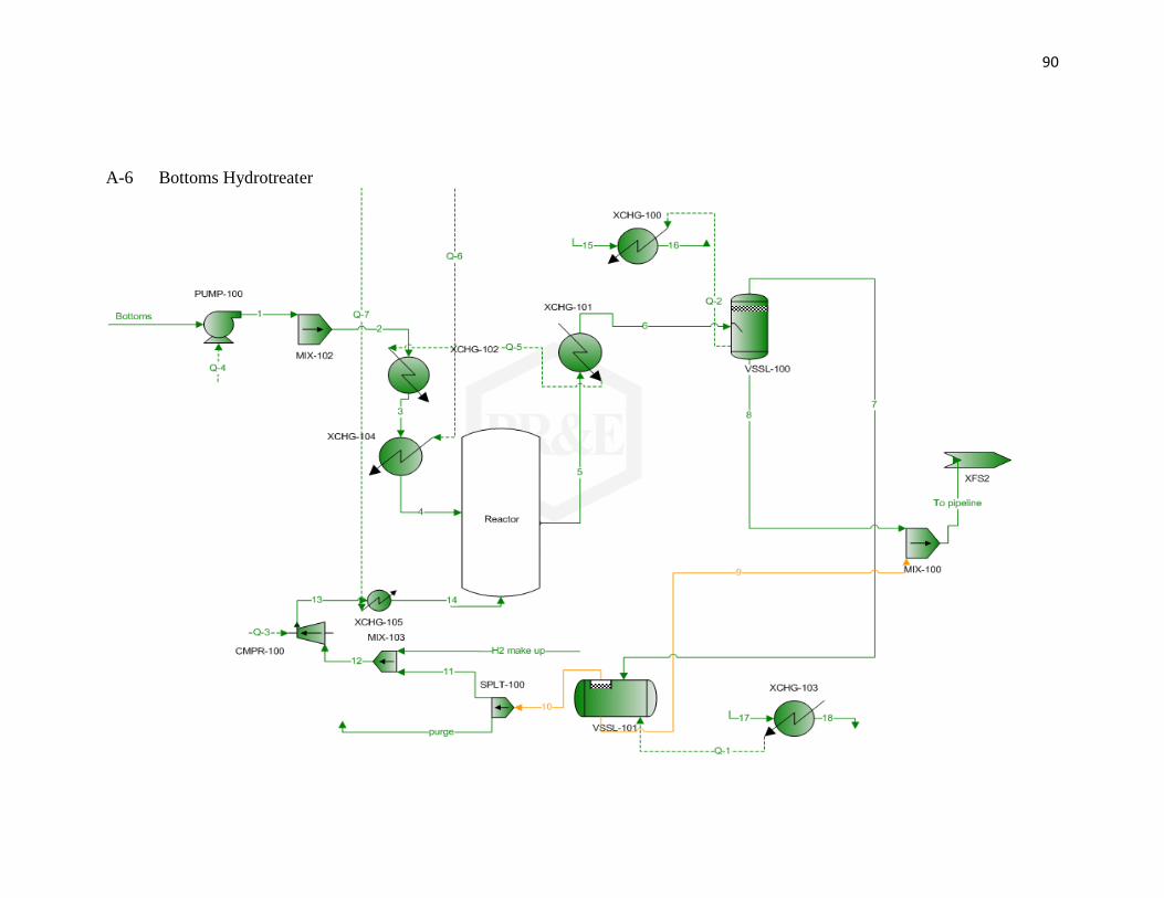
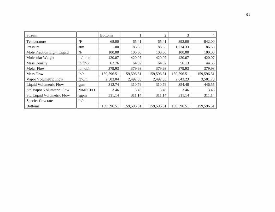
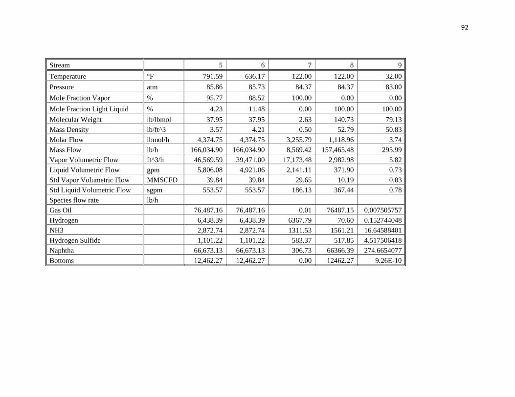
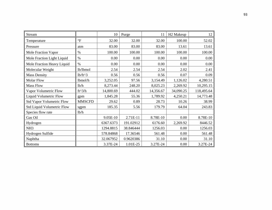
equilibrium in favor of the reactants. A more detailed process flow sheet with a table for
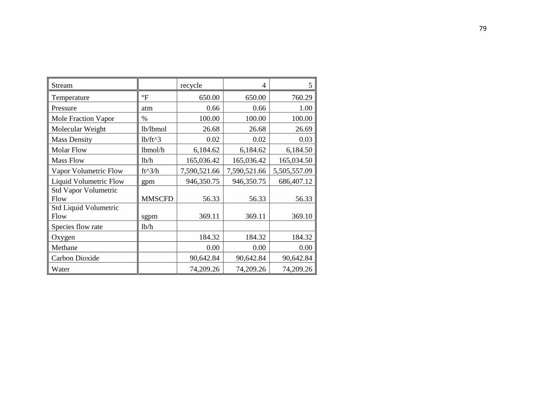
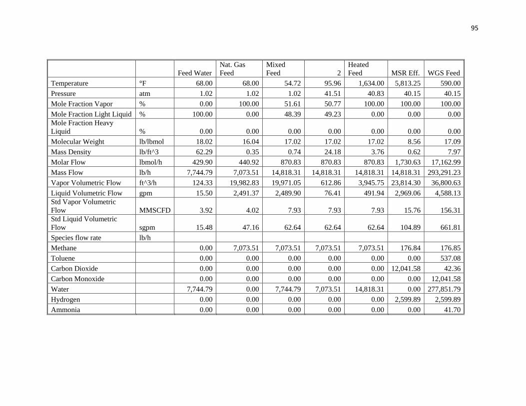
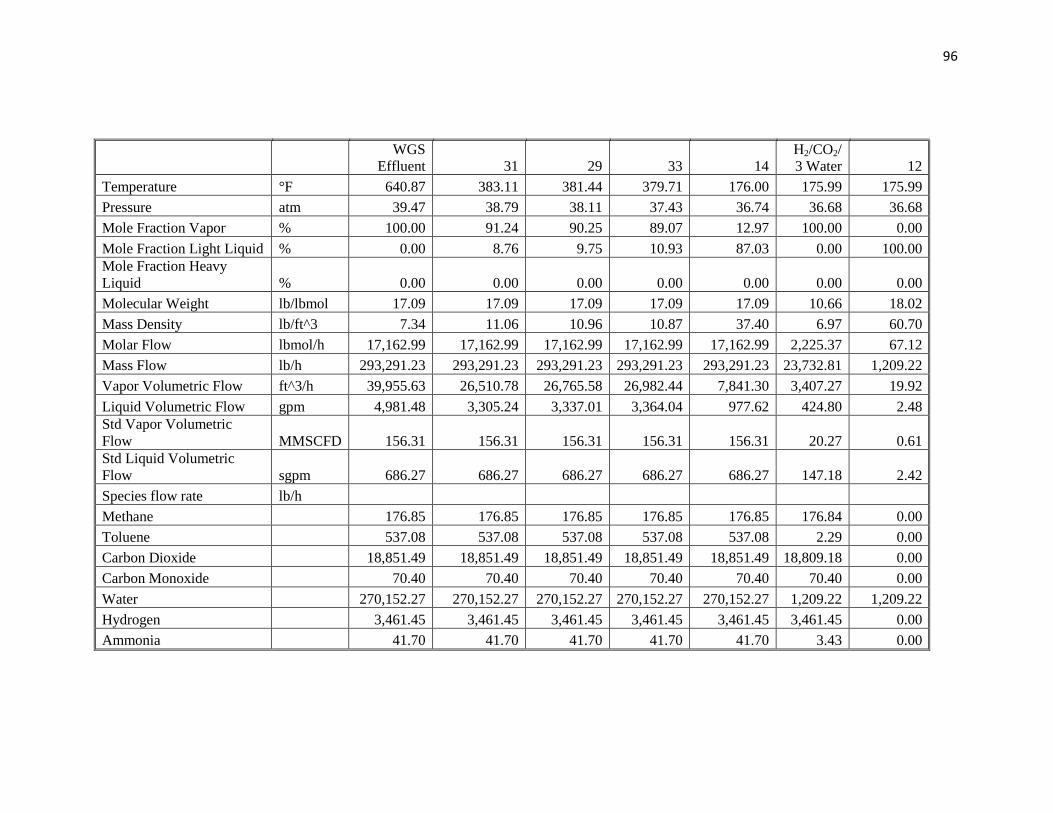
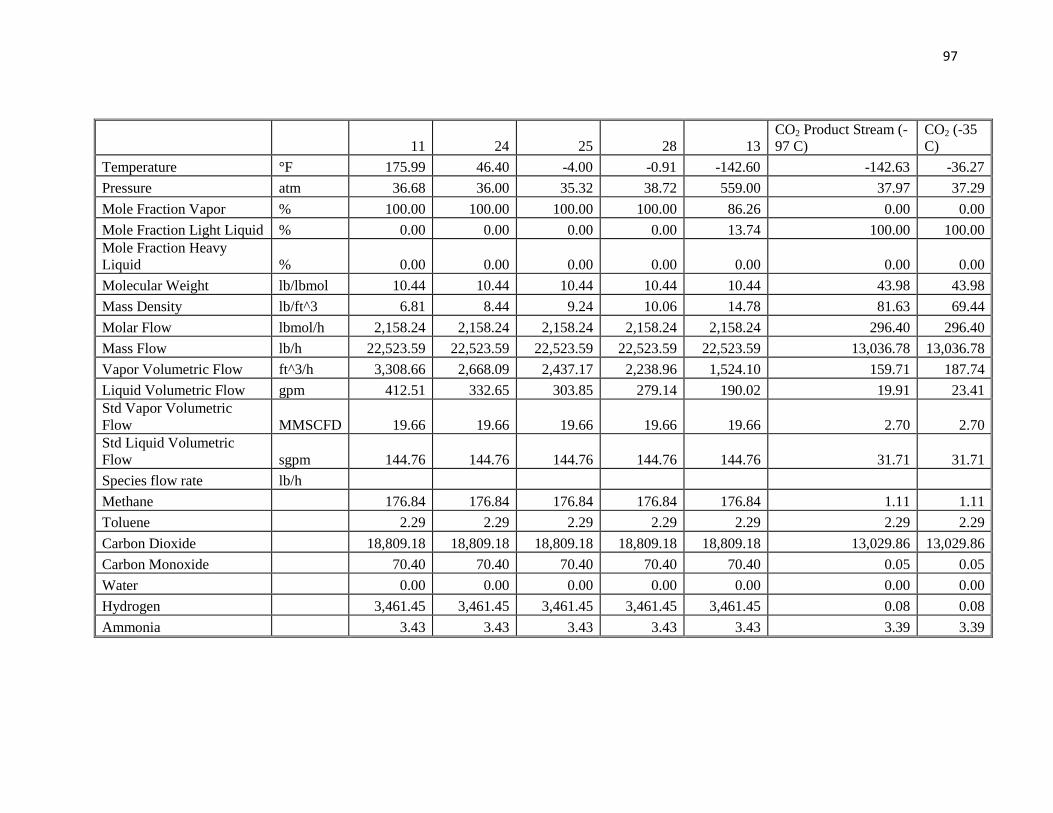
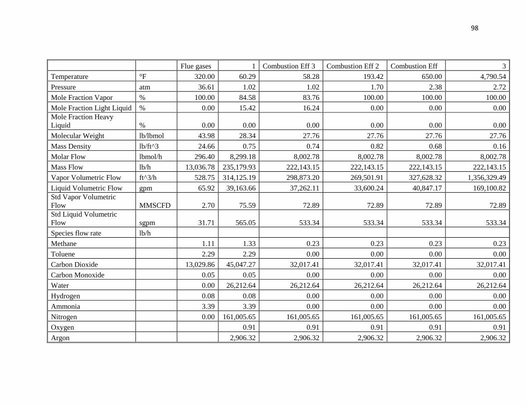
properties and composition of each stream is given in Appendix A-6.
Page 49
38
Figure 13: Mass flow rates of each component in the Water-Gas shift Reactor as a
function of distance down the reactor (shown in 10 increments)
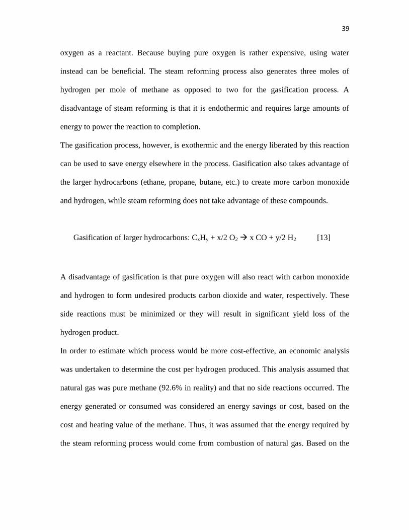
2.3.5.4 Gasification vs. Steam Reforming
Natural gas can be converted to hydrogen and carbon monoxide by two different
reactions: methane steam reforming or gasification. Each reaction forms hydrogen and
carbon monoxide with the reactions shown below:
Because either process seemed to be a viable candidate for hydrogen production, a study
was undertaken to select a reaction before any system design was begun. Each process
has advantages and disadvantages. Steam reforming of methane uses water, rather than
Gasification: CH4 + ½ O2 CO + 2 H2 [11]
Steam Reforming: CH4 + H2O → CO + 3H2 [12]
Page 50
39
oxygen as a reactant. Because buying pure oxygen is rather expensive, using water
instead can be beneficial. The steam reforming process also generates three moles of
hydrogen per mole of methane as opposed to two for the gasification process. A
disadvantage of steam reforming is that it is endothermic and requires large amounts of
energy to power the reaction to completion.
The gasification process, however, is exothermic and the energy liberated by this reaction
can be used to save energy elsewhere in the process. Gasification also takes advantage of
the larger hydrocarbons (ethane, propane, butane, etc.) to create more carbon monoxide
and hydrogen, while steam reforming does not take advantage of these compounds.
Gasification of larger hydrocarbons: CxHy + x/2 O2 x CO + y/2 H2 [13]
A disadvantage of gasification is that pure oxygen will also react with carbon monoxide
and hydrogen to form undesired products carbon dioxide and water, respectively. These
side reactions must be minimized or they will result in significant yield loss of the
hydrogen product.
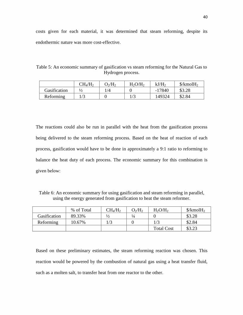
In order to estimate which process would be more cost-effective, an economic analysis
was undertaken to determine the cost per hydrogen produced. This analysis assumed that
natural gas was pure methane (92.6% in reality) and that no side reactions occurred. The
energy generated or consumed was considered an energy savings or cost, based on the
cost and heating value of the methane. Thus, it was assumed that the energy required by
the steam reforming process would come from combustion of natural gas. Based on the
Page 51
40
costs given for each material, it was determined that steam reforming, despite its
endothermic nature was more cost-effective.
Table 5: An economic summary of gasification vs steam reforming for the Natural Gas to
Hydrogen process.
CH4/H2 O2/H2 H2O/H2 kJ/H2 $/kmolH2
Gasification ½ 1/4 0 -17840 $3.28
Reforming 1/3 0 1/3 149324 $2.84
The reactions could also be run in parallel with the heat from the gasification process
being delivered to the steam reforming process. Based on the heat of reaction of each
process, gasification would have to be done in approximately a 9:1 ratio to reforming to
balance the heat duty of each process. The economic summary for this combination is
given below:
Table 6: An economic summary for using gasification and steam reforming in parallel,
using the energy generated from gasification to heat the steam reformer.
% of Total CH4/H2 O2/H2 H2O/H2 $/kmolH2
Gasification 89.33% ½ ¼ 0 $3.28
Reforming 10.67% 1/3 0 1/3 $2.84
Total Cost $3.23
Based on these preliminary estimates, the steam reforming reaction was chosen. This
reaction would be powered by the combustion of natural gas using a heat transfer fluid,
such as a molten salt, to transfer heat from one reactor to the other.
Page 52
41
2.3.5.4 Environmental Assessment of Hydrogen Plant
A number of methods have been proposed by Allen and Shonnard (Allen D.T., 2002) for
quantifying the environmental impact of chemical processes. Typically the first step in
comparing the environmental impact of a process is to compute the processes
environmental index (EI) based on toxicity:
(
) [14]
where νi is the stoichiometric coefficient of species i and TFi is a toxicity factor (usually
the threshold limit value, TLV, or permissible exposure limit, PEL) for the compound.
Unfortunately implementation of this initial approach is complicated by all of the
different reactions considered in each process flow sheet, and isn‟t particularly useful
because each process involves almost exactly the same chemical species. Even without
performing any calculations, it is clear that according to Equation 14 the steam reforming
process will be more environmentally friendly than gasification of shale oil because of
the heavier hydrocarbons and sulfur content of the shale oil feed.
A more applicable method developed by Allen and Shonnard (Allen D.T., 2002) is to
compare the mass, and emissions required to produce a unit of product. Using 1lb of H2
product as the basis for comparison, steam reforming and gasification of shale oil are
compared below in Table 7 (the data used in the analysis below was taken from each
process flow sheet):
Page 53
42
Table 7: Environmental comparison of steam reforming and shale oil gasification.
Emissions include all gaseous products except CO2.
Process
Intensities (lb/lb H2)
Material Water CO2 Emissions
Steam Reforming 9.71 1.02 9.49 0.22
Shale Oil
Gasification
14.66 2.41 13.76 0.96
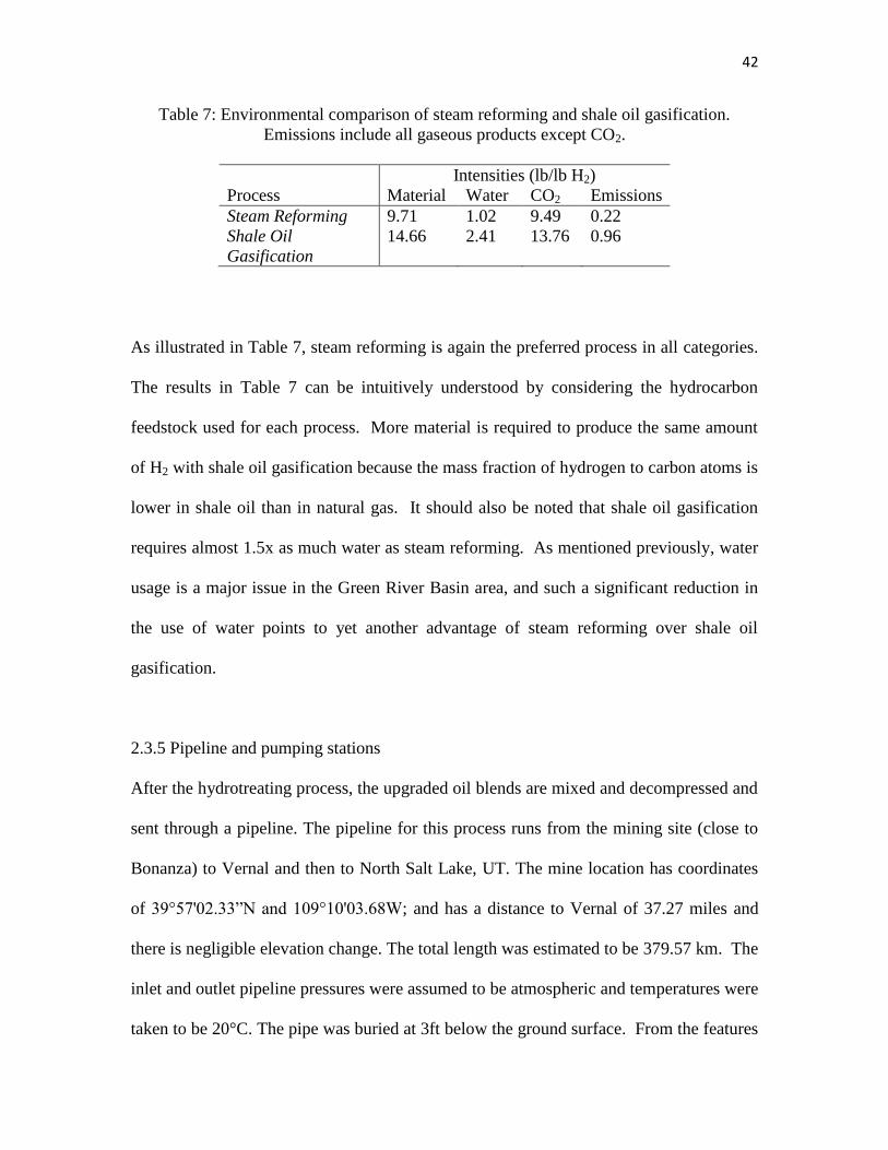
As illustrated in Table 7, steam reforming is again the preferred process in all categories.
The results in Table 7 can be intuitively understood by considering the hydrocarbon
feedstock used for each process. More material is required to produce the same amount
of H2 with shale oil gasification because the mass fraction of hydrogen to carbon atoms is
lower in shale oil than in natural gas. It should also be noted that shale oil gasification
requires almost 1.5x as much water as steam reforming. As mentioned previously, water
usage is a major issue in the Green River Basin area, and such a significant reduction in
the use of water points to yet another advantage of steam reforming over shale oil
gasification.
2.3.5 Pipeline and pumping stations
After the hydrotreating process, the upgraded oil blends are mixed and decompressed and
sent through a pipeline. The pipeline for this process runs from the mining site (close to
Bonanza) to Vernal and then to North Salt Lake, UT. The mine location has coordinates
of 39°57'02.33”N and 109°10'03.68W; and has a distance to Vernal of 37.27 miles and
there is negligible elevation change. The total length was estimated to be 379.57 km. The
inlet and outlet pipeline pressures were assumed to be atmospheric and temperatures were
taken to be 20°C. The pipe was buried at 3ft below the ground surface. From the features
Page 54
43
of the oil and the environment, it was estimated that an economical pipeline diameter
could be 12 inches. The material of the pipe was assumed to be Carbon Steel A134.
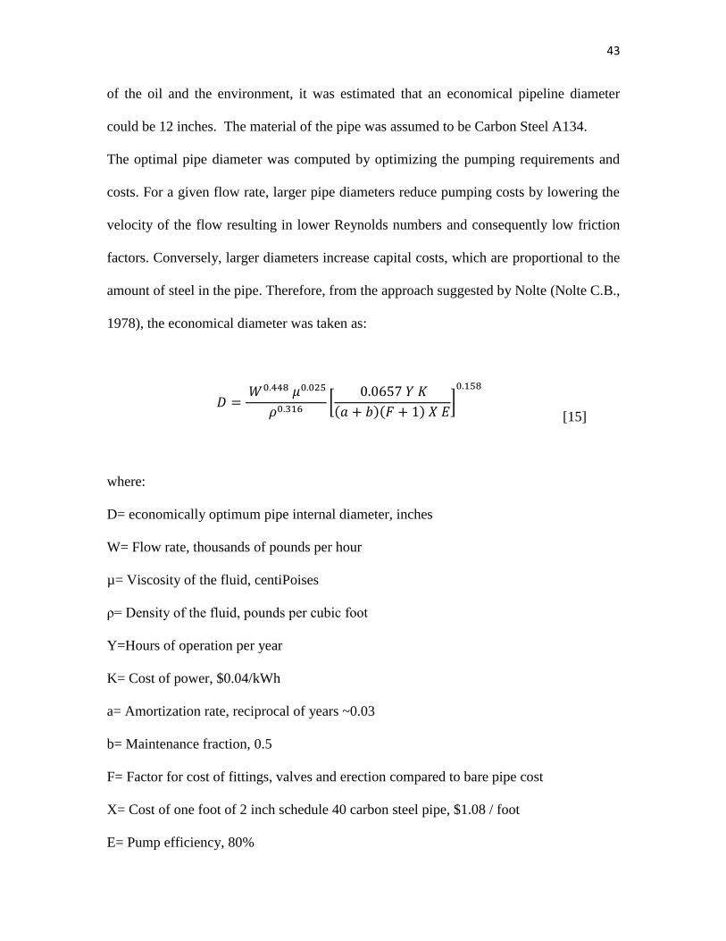
The optimal pipe diameter was computed by optimizing the pumping requirements and
costs. For a given flow rate, larger pipe diameters reduce pumping costs by lowering the
velocity of the flow resulting in lower Reynolds numbers and consequently low friction
factors. Conversely, larger diameters increase capital costs, which are proportional to the
amount of steel in the pipe. Therefore, from the approach suggested by Nolte (Nolte C.B.,
1978), the economical diameter was taken as:
[
( )( ) ]
[15]
where:
D= economically optimum pipe internal diameter, inches
W= Flow rate, thousands of pounds per hour
µ= Viscosity of the fluid, centiPoises
ρ= Density of the fluid, pounds per cubic foot
Y=Hours of operation per year
K= Cost of power, $0.04/kWh
a= Amortization rate, reciprocal of years ~0.03
b= Maintenance fraction, 0.5
F= Factor for cost of fittings, valves and erection compared to bare pipe cost
X= Cost of one foot of 2 inch schedule 40 carbon steel pipe, $1.08 / foot
E= Pump efficiency, 80%
Page 55
44
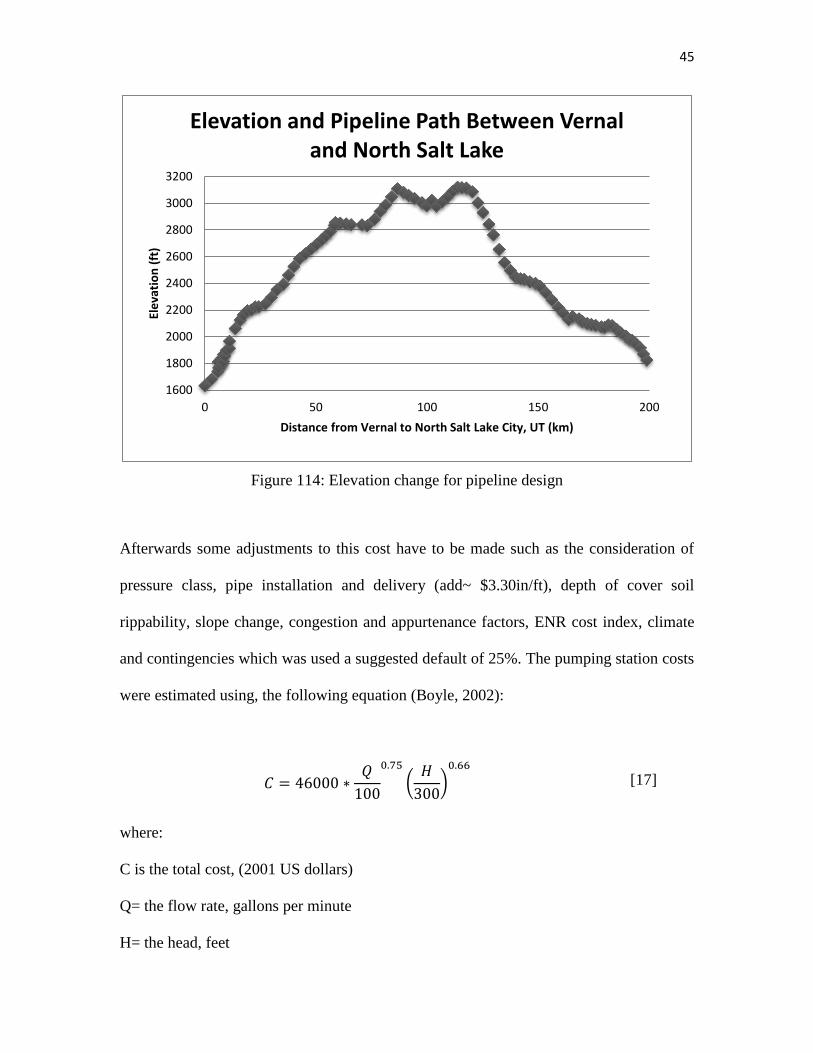
For higher accuracy in the simulation, it is necessary to consider any elevation change in
the selected route (See Figure 14). From Vernal to mile 71, an average inclination angle
of 0.013° was calculated; while the remaining distance was specified with an inclination
angle of -0.0196.
The pumping requirements were automatically calculated to overcome any inclination,
friction and oil hold ups by the use of standardized centrifugal pumps. Based on the
maximum designable pumps (Seider W.D., 2004) a total of four pumping stations were
required.
The costs for the pipe and the pumping stations were computed based on Boyle„s
methodology (Boyle, 2002), which consisted of different steps. The first step required for
this method is to get a base pipe cost in dollars (July 1992) per diameter-inch per lineal
foot ($/in/ft), using the following equation:
( ) [16]
Page 56
45
Figure 114: Elevation change for pipeline design
Afterwards some adjustments to this cost have to be made such as the consideration of
pressure class, pipe installation and delivery (add~ $3.30in/ft), depth of cover soil
rippability, slope change, congestion and appurtenance factors, ENR cost index, climate
and contingencies which was used a suggested default of 25%. The pumping station costs
were estimated using, the following equation (Boyle, 2002):
(
)
[17]
where:
C is the total cost, (2001 US dollars)
Q= the flow rate, gallons per minute
H= the head, feet
1600
1800
2000
2200
2400
2600
2800
3000
3200
0 50 100 150 200
Ele
vati
on
(ft
)
Distance from Vernal to North Salt Lake City, UT (km)
Elevation and Pipeline Path Between Vernal and North Salt Lake
Page 57
46
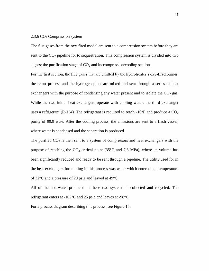
2.3.6 CO2 Compression system
The flue gases from the oxy-fired model are sent to a compression system before they are
sent to the CO2 pipeline for to sequestration. This compression system is divided into two
stages; the purification stage of CO2 and its compression/cooling section.
For the first section, the flue gases that are emitted by the hydrotreater‟s oxy-fired burner,
the retort process and the hydrogen plant are mixed and sent through a series of heat
exchangers with the purpose of condensing any water present and to isolate the CO2 gas.
While the two initial heat exchangers operate with cooling water; the third exchanger
uses a refrigerant (R-134). The refrigerant is required to reach -10°F and produce a CO2
purity of 99.9 wt%. After the cooling process, the emissions are sent to a flash vessel,
where water is condensed and the separation is produced.
The purified CO2 is then sent to a system of compressors and heat exchangers with the
purpose of reaching the CO2 critical point (35°C and 7.6 MPa), where its volume has
been significantly reduced and ready to be sent through a pipeline. The utility used for in
the heat exchangers for cooling in this process was water which entered at a temperature
of 32°C and a pressure of 20 psia and leaved at 49°C.
All of the hot water produced in these two systems is collected and recycled. The
refrigerant enters at -102°C and 25 psia and leaves at -98°C.
For a process diagram describing this process, see Figure 15.
Page 58
47
Figure 125: Process Flow Diagram for CO2 Compression System
Page 59
48
2.3.7 Water Reservoir
The extraction and upgrading process requires water on a daily basis as well as a one time
supply to fill tanks to start up operations. Due to the requirement for the process plants
need to operate “24-7” over an annual operating schedule of 330 days/y, water for the
various processes especially for steam generation must be available. Water is estimated
to cost $50/ac-ft/yr in this region. It must be purchased from other users since there are in
the region. Since water is a scarce commodity in this arid region of the west, a reservoir
is needed. The reservoir will be filled by either pumping water from the aquifer or by
diversion of the Green River in the area to fill the reservoir. The size of this reservoir
needs to be is determined by the duration of a prolonged drought in the area. While this
study has not done and sophisticate analysis of the hydrology of the Green River basin,
we have taken a look at historical periods of drought as defined as between the rain
storms over the basin and find that 90 days or the duration of the summer is reasonable as
a worst case for water storage. As a result total water utilization for the process 3500 ac-
ft/y for the air-fired combustion heating case and the need for a 90 day supply, the size of
the reservoir is determined. From the size of the reservoir the cost can be determined
using construction excavation costs that are applicable in this part of the state of Utah
(RSMeans, 2002). The cost of a water reservoir for this operation is substantial as we will
see.
2.3.8 Utility Plants
Each of the utilities used throughout the processes requires a source; for that reason,
utility plants, pipelines, electric lines and others were sited and their costs were estimated.
Page 60
49
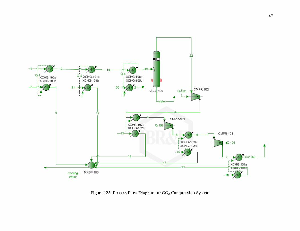
The costs for the substations were computed based on Seider‟s methodology (Seider
W.D., 2004); where the investment costs were related to the rate of usage for each facility
(Table 8.)
Table 8: Allocated Capital Investment Costs (Seider W.D., 2004)
Utility Capital Cost Rate
Steam $50/(lb/hr)
Electricity $203/kW
Cooling Water $58/gpm
Process Water $347/gpm
Refrigeration $1,330/ton
Liquid waste disposal $3/1,000gpy
Additionally, the costs for the electric and gas lines were assumed to be $425,000/mile
and $200.00/ft respectively, the electric switching, gear and tab $10,000/mile and the
meter and regulation facility for natural gas $1,000,000. The location to the closest
service facility was assumed to be in Bonanza UT (about 5 miles).
Page 61
50
CHAPTER 3
EQUIPMENT SIZE AND COSTING PROCEDURES
3.1 Introduction
In order to determine the economic viability of the processes and scenarios described
above, it was necessary to calculate annual cash flows. These cash flows were estimated
for each year for period of twenty years. These cash flows were calculated as follows:
[18]
( ) [19]
where:
CF= Annual cash flow
Cv= Variable operating costs
CTDC=Total depreciable capital
CS=Cost of start up
P= Production capacity (days operated/yr)
Cf= Fixed operating costs
Page 62
51
CWC =Working capital
CR= Cost of royalties
S=Total gross sales
T=Taxes
CL=Cost of land
Sequip= Equipment salvage
T=Corporate tax rate
d=Depletion
D=Depreciation
Each term represents the amount of revenue or costs in that category in a given year. The
present value (PV) of the cash flow in each year of project was determined by applying
the discount factor:
[
( ) ] [20]
which adjusts the cash flow in the n-th year of a project according to an annually
compounded interest rate (representing the time-value of money for the entity financing
the project). The net present value (NPV is the summation of each year‟s present value
cash flow) and the internal rate of return (IRR is the interest rate that results in NPV =
0) for each scenario were computed to assess profitability. Individual terms in Eq. [16] –
[20] was evaluated as discussed below.
Page 63
52
3.2 Capital Costs
Capital costs for project were estimated using a combination of two techniques, namely
Williams six-tenths rule (Williams R., 1947)for economy of scale and the individual
factors method of Guthrie (Guthrie K.M., 1974).
According to Williams (Williams R., 1947), economies of scale in chemical processes
(for everything from individual pieces of equipment to entire plants) can be described by
Eq. [21]:
(
)
(
) [21]
where C is cost, Q refers to a material capacity (oil production rate, raw shale processed,
etc.), m is a scaling power, is an appropriate cost index (CE Plant Index, Producers
Price Index, etc.), and the subscript “o” refers to the base value of the subscripted
variable. Equation [21] is referred to as the “six-tenths rule” because Williams (1947)
found that on average the best fit to cost data was given by m = 0.6, and for the purposes
of this study it was assumed that m = 0.6 for all capital costs (Eq. (21) was also used in
some instances for estimating annual costs in which case m = 1, see the discussion of
annual costs below). Williams (1947) six-tenths rule was applied in the ex-situ oil shale
scenario to scale the capital costs and processing data for mining and retorting from
Weiss (1982), whose work estimated the costs for producing 46,400 bbl/day of crude oil
from oil shale using the TOSCO II process.
The individual factor method of Guthrie (1974) gives preliminary estimates of the CTDC
of a project based on the sum of the purchase costs (CP) of individual pieces of equipment
Page 64
53
multiplied by a series of factors to give a bare-module cost (CBM, which accounts for the
total direct (CP) and indirect (delivery, insurance, taxes, installation, etc.) costs of process
equipment):
∑ ∑[ (
) [ ( )]]
[20]
where each factor is:
FBM = Bare-module factor
Fd = Design factor
FP = pressure factor
FM = material factor
Optimized process designs (including mass and energy balances, equipment sizing, and
construction materials selection) were generated for the upgrading (hydrotreater and H2
generation plant) and delivery (pipeline) portions of each scenario using ProMax (a
process flow sheet simulator), which allowed for estimation of CP from cost data given
by (Seider W.D., 2004) using the sizing factors specified in Table 9
Page 65
54
Table 9: Size factor for equipment cost
UNIT SIZE FACTOR COMMENTS
Trickle-bed reactor LHSV NiMo/Al2O3 Catalyst, kinetics from
Botchwey (2004)
Pumps Change in Pressure
Heat Exchangers Area
Flash Separator Residence Time
Compressors Horse Power
Furnace Heat Duty
Steam Reformer Residence Time Cu/Zn Catalyst
Water Shift Reactor Residence Time Fe/Cr2O3 Catalyst
Holding Tank Volume
Taken together, the combination of Williams six-tenths rule and the method of Guthrie
provided reasonable estimates of the total depreciable capital cost (CTDC) fot each
scenario. Other capital costs, such as the cost of working capital, land, startup, and
salvage were estimated as percentages of CTDC as recommended by Seider (Seider W.D.,
2004). Additional data and algorithms for estimating capital costs were used for offsite
facilities not typically associated with the chemical industry. RSMeans heavy
construction cost data was used to estimate the cost of building a reservoir for process
water (RSMeans, 2002), and the approach suggested by Seider (Seider W.D., 2004) was
followed for approximating the cost of delivery pipelines.
3.3 Annual Costs
The annual costs in each scenario can be differentiated into fixed (CF) and variable (CV)
costs based on whether they are or are not a function of the process being in operation.
Page 66
55
Variable costs in our scenarios are defined as a combination of utilities (water, fuel,
electricity, etc.) and other expenses related indirectly to production (sales, research,
administration, etc.). Utility requirements were either taken directly from the appropriate
process design flow sheet or scaled from base scenario process data (Weiss M.A., 1982)
for ex-situ oil shale mine and retort) using a variant of Eq. [21]
(
)
[21]
where U is the utility requirement and all other variables are the same as in Eq. (19),
except that the scaling exponent m is always set to m = 1. Most utility costs were
estimated from price data given by Seider (Seider W.D., 2004), with supplementary price
data coming from the EIA (2010), the Uintah Water Conservancy District (2010), and
others. Estimates for indirect annual expenses were also derived according to Seider‟s
recommendations.
The fixed expenses in the scenarios were assumed to be the cost of labor, property taxes,
and insurance, all of which were estimated according to Seider who also suggested that
property taxes and insurance were assumed to be a percentage of CTDC (Seider W.D.,
2004). Labor was assumed to be a fixed expense because the large amount of manpower
required during plant maintenance and downtime implies that operational labor would be
participating in work during shut downs. Labor related to operations was estimated
according to assumed hourly wages and the number of operators required for a sequence
of process units based on the type of process (solids/fluids) that they handled and their
Page 67
56
throughput. Maintenance related labor was estimated as a percentage of CTDC, again
based upon the type of process handled.
3.3.1 Cost of Utilities to Operate Ex Situ Oil shale Extraction and Upgrading
Utilities for this process are numerous. A list of utilities and their prices used for the ex
situ extraction and upgrading of oil shale is given in Table 10.
3.4 Sales
Oil sales are calculated for each year of the project based on EIA (2010) forecasts. The
sales price we have assumed for oil represents the refiner's acquisition price of imported
low sulfur light crude given in the EIA‟s forecast. In addition to the sales revenue
generated by oil, several scenarios also considered the possibility of implementing CO2
capture. In these scenarios free on board (f.o.b.) supercritical CO2 sale for enhanced oil
recovery (EOR) is included in each year‟s sales revenue at an assumed price of $25/ton.
3.5 Taxes and Royalties
The total corporate state and federal taxes paid each year are calculated using Eq. [19].
Net income is calculated by subtracting all operating costs, depreciation, and depletion
from gross sales revenue. Depreciation of CTDC is assumed to follow a 10 year Modified
Accelerated Cost Recovery System (MARCS) schedule. If a given scenario involves a
private land purchase for extracting oil and gas, then an additional deduction can be made
for depletion (assumed to be 15% of gross income).
Royalties were assumed to start at 5% and increase up to 12.5% over a period of 10 years
(Keiter R. B., 2009)
Page 68
57
Table 10: Utility Prices used for Ex Situ Extraction and Upgrading for Oil Shale
Utilities
Fuel (natural gas) $ 4.27 per MBtu
Electricity $ 0.04 per kWh
Water
Raw water $ 50.00 / (acre-ft * yr)
$ 16,292.55 / (k gal * yr)
Water Storage 90 days
Water recycle loses 3%
Boiler feed water $ 1.50 / k gal
Process water $ 0.50 / k gal
Cooling water $ 0.05 / k gal
Steam $ 5.50 / k lbs
Oxygen $ 70.00 / ton
Catalyst $ 4.24 /kg
CO2
Tax Rate $ 25.00 / ton CO2
Sale Rate $ 25.00 / ton CO2
Refrigerants
Ethylene: -150 deg(F) $ 10.50 / GJ
R-134a: -30 deg(F) $ 6.60 / GJ
Chemicals $ 75.00 / kg
Plant Utilization 330 days / year
Page 69
58
CHAPTER 4
OPERATING COST AND ECONOMIC ANALYSIS
4.1 Air-fired Case
4.1.1 Capital Costs
The base case scenario for the oil shale production (quality of the rock of 25 gal/ton)
revealed a total depreciable capital for this plant of $3.34 Billion. The largest capital costs
are mining and retorting (71%), hydrotreater (23%), oil pipeline (4.8%) and utility plants
(0.65%) in that order; along with only 1.08% which consist on the hydrogen plant, utility
plants and the water reservoir. Figure 16 contains a pie chart of where the capital
expenditures are depicted; while Table 11 contains the costs for each section of the
process.
Additionally, the cases where the shale quality was 20 gal/ton and 35 gal/ton revealed
capital costs of $3.64 and $2.97 Billion respectively. These results are reasonable; it was
expected that the higher the quality of the rock the less mining would be performed, and
thus the cheaper the overall process.
Page 70
59
Figure 136: Pie chart of capital costs for Ex Situ Oil Shale Extraction and Upgrading for
Air-Fired Plant Heat Requirements
Table 11: Air-Fired Process Total Depreciable Capital for 25 gal/ton case
Hydrotreater $ 722,827,249.63 23.21%
Pipeline $ 148,923,634.96 4.78%
H2 Plant $ 11,200,985.49 0.36%
Mine and Retort $ 2,229,060,359.91 71.58%
Water Reservoir $ 2,172,261.83 0.07%
Utility Plants $ 20,224,670.92 0.65%
Subtotal $ 3,114,184,491.82 100.00%
Total $ 3,345,615,982.09
Hydrotreater
Pipeline
H2 Plant
Mine and Retort
Water Reservoir
Utility Plants
Air-fired Case Depreciable Capital ($3.3 Billion, 25 gal/ton)
Page 71
60
4.1.2 Annual sales and Costs
The total annual operating costs for the 25 gal/ton case was estimated at $984 million
with $439 million in fixed costs and $545 million in variable costs. Among these annual
costs, the highest costs are labor (38%), general expenses (24%) and fuel (19%). Note
that general expenses consist on sales expenses, direct research, allocated research,
administrative expenses and incentives
Revenues for the base case and its variants are presented in Figure 17. Here we see two
bars, one for revenue (R) and the other for costs (C) for this base case. As can be seen
comparing the “R” and “C” bars, the revenue and the costs are equal, as they should be.
The variable and fixed costs to produce the syn crude oil are broken down in the C bar.
Starting from the top C-Base bar we find that the largest costs are for Profit (ROI) due
investors corresponding to $30.31/bbl to earnings, $29.88/bbl of variable annual costs,
federal taxes (assuming that the full rates are paid) corresponding to $16.13/bbl, and
$12.51/bbl for royalties, plant startup, and land. The annual fixed costs correspond to
$12.36/bbl; while the interest charges on the total depreciable capital is $11.11/bbl.
There are other subcategories within the variable cost, being general expenses such as
direct and allocated research, management incentive compensations and administrative
expense at 43.41 % and fuel (natural gas) at 34.3% the biggest. For the base case, these
costs are broken down into percentages of the total variable cost in the pie chart shown in
Figure 18 and Table 12
Page 72
61
Figure 147: Revenue and Cost of Ex Situ Oil Shale Extraction and Upgrading for Air-Fired Plant Heat Requirements–Variable Grade
of Oil Shale
$112.31
$124.47
$97.27
$114.65
$11.11 $12.10 $9.86 $11.11
$29.88 $34.26
$24.75 $31.97
$12.36
$13.23
$11.16
$11.90
$12.51
$13.86
$10.84
$12.76
$30.31
$33.38
$26.46
$30.68
$16.13
$17.66
$14.21
$16.23
$-
$20.00
$40.00
$60.00
$80.00
$100.00
$120.00
$140.00
R-25 Gal/Ton C-25 Gal/Ton R-20 Gal/Ton C-20 Gal/Ton R-35 Gal/Ton C-35 Gal/Ton R-25 Gal/Ton wCO2 tax
C-25 Gal/Ton wCO2 tax
$/b
bl
Value of Revenue and Supply Cost Components
Oil Sales Total Depreciable Capital Variable Annual Costs Fixed Annual Costs Other Earnings Taxes
Page 73
62
Figure 158: Air-fired variable costs distribution for the 25 gal/ton case
Table 12: Variable Costs ($/bbl) for the 25 gal/ton case
Catalyst 0.088722787 0.30%
Chemicals (for retort) 0.11618298 0.39%
Desiccant 0.005147019 0.02%
Electricity 0.63539119 2.13%
General Expenses 12.97156588 43.41%
Fuel 10.24745691 34.29%
Mining 2.455827766 8.22%
Refrigerant 0.019035786 0.06%
Steam 0.3741696 1.25%
Water 2.966986593 9.93%
Total 29.88048651 100.00%
Catalyst
Chemicals (for retort)
Desiccant
Electricity
General Expenses
Fuel
Mining
Refrigerant Steam
Water
Variable Costs, ($29.9/bbl, 25 gal/ton)
Page 74
63
The base case scenario revealed a cost of $112/bbl, with a return on investment (ROI) of
18% and a payback period of 3.56 years. Returning to Figure 17 we can see the impact of
the oil shale grade on the supply costs. As the oil shale grade goes down to 20 gal/ton
and up to 35 gal/ton the supply costs increase to $124/bbl and decrease to $97/bbl,
respectively.
Tax on CO2 increases the base case scenario supply cost by 1.75% or $114.65/bbl. This
increase is reflected in a 3.7% increase in the total annual operating costs, which is
$1,022 million.
4.2 Oxy-fired Case
4.2.1 Capital Costs
Using the same average mined oil shale grade of 25 gal/ton as in the air-fired case, but
with an oxy-fired combustion for plant heating requirements and compression and sales
of CO2 for EOR or other sequestration; the Base Ex Situ Case was developed.
The total depreciable capital for this plant is $3.39 Billion. The capital costs are
categorized as retorting and mining (70.8%), hydrotreater (23%), water reservoir (11%)
and oil pipeline (3.3%) in that order. The CO2 compression plant and hydrogen plant are
much smaller, corresponding to 0.96% and 0.29% respectively. Note that for the air case,
there wasn‟t a CO2 compression plant. The relative capital expenditures are summarized
in Figure 19. Table 13 contains the costs for each part of the process.
The variation of oil shale grade again shows higher capital costs for the lower grade cases
and vice versa; $3.69 and $3.00 Billon for the 20 gal/ton and 35 gal/ton case,
respectively.
Page 75
64
4.2.2 Annual sales and Costs
The total annual operating costs for this case were calculated to be $1,160 million with
$445 million corresponding to fixed costs and $715 million in variable costs. Among
these annual costs, the highest costs are labor (32%), fuel (26%) and general expenses
(22%). Moreover, oxygen had to be included as a new utility cost; it consisted of 10.8%
of the total annual costs.
Again, to provide a sensitivity analysis for the oil shale grade, revenues for the base case
and its variants are presented in Figure 20. The top C-Base bar from the base scenario we
find that the largest costs for Profit (ROI) which consist on $39.4/bbl being the variable
annual costs, followed by earnings $32/bbl and Taxes $17/bbl. While the annual fixed
costs corresponded to $10.78/bbl and a total depreciable capital of $11.27/bbl; the
revenue due to selling CO2 turned out to be $1.8/bbl. The biggest subcategories within
the variable cost were the general expenses (36.3 %) and fuel (25.9%). For this base
case, these costs were broken into percentages of the total variable cost as shown in
Figure 21.
The base case scenario revealed a cost of $122/bbl, with a return on investment (ROI) of
18% and a payback period of 3.59 years. The impact of the oil shale grade on the supply
costs are presented in this case too. As the oil shale grade goes down to 20 gal/ton and up
to 30 and 35 gal/ton the supply costs increased to $135/bbl and decreased to $112/bbl and
$105/bbl respectively.
Page 76
65
Figure 169: Pie chart of capital costs for Ex Situ Oil Shale Extraction and Upgrading for
Oxy-Fired Plant Heat Requirements
Table 13: Oxy-Fired Process Total Depreciable Capital
Hydrotreater $ 727,324,018.44 23.11%
Pipeline $ 148,923,634.96 4.73%
H2 Plant $ 9,116,149.51 0.29%
Mine and Retort $ 2,229,060,359.91 70.82%
Utility Plants $ 26,536,602.76 0.84%
Water Reservoir $ 2,582,680.08 0.08%
CO2 Compressor $ 30,301,681.09 0.96%
Subtotal $ 3,147,308,523.99 100.00%
Total $ 3,391,571,793.51
Hydrotreater
Pipeline
H2 Plant
Mine and Retort
Utility Plants
Water Reservoir CO2 Compressor
Oxy-fired Depreciable Capital ($3.4 Billion, 25 gal/ton)
Page 77
66
Figure20: Revenue and Cost of Ex Situ Oil Shale Extraction and Upgrading for Oxy-Fired Plant Heat Requirements–Variable Grade
of Oil Shale
$122.09
$135.80
$112.47 $105.29
$11.27 $12.27 $10.54 $9.99
$39.40 $45.34
$35.38 $32.48
$10.78
$11.48
$10.25 $9.81
$13.57
$15.08
$12.50 $11.71
$32.16
$35.40
$29.84
$28.08
$16.68
$18.28
$15.53
$14.67
$1.77
$2.05
$1.58
$1.45
$-
$20.00
$40.00
$60.00
$80.00
$100.00
$120.00
$140.00
$160.00
R-25 Gal/Ton C-25 Gal/Ton R-20 Gal/Ton C-20 Gal/Ton R-30 Gal/Ton C-30 Gal/Ton R-35 Gal/Ton C-35 Gal/Ton
$/b
bl
Value of Revenue and Supply Cost Components
Oil Sales Total Depreciable Capital Variable Annual Costs Fixed Annual Costs Other Earnings Taxes CO2 Sales
Page 78
67
Figure 171: Oxy-fired variable costs distribution for the 25 gal/ton base case
Table 14: Variable Costs ($/bbl) for the 25 gal/ton case
Catalyst 0.088729009 0.23%
Chemicals (for retort) 0.11618298 0.29%
Desiccant 0.005145813 0.01%
Electricity 1.147805834 2.91%
General Expenses 14.30548136 36.31%
Fuel 10.22430808 25.95%
Mining 2.455827766 6.23%
O2 6.8825931 17.47%
Refrigerant 0.172320189 0.44%
Steam 0.3741696 0.95%
Water 3.62707739 9.21%
Total 39.39964112 100.00%
Catalyst Chemicals (for
retort)
Desiccant
Electricity
General Expenses
Fuel
Mining
O2
Refrigerant Steam
Variable Costs, ($39.4/bbl, 25 gal/ton)
Page 79
68
4.3 Oxy vs Air-Fired Burners
The presented results clearly show that oxy-fired burners with a CO2 compression system
entail high costs. For a base case scenario of 25 gal/ton without CO2 taxation, the cost for
an air-fired process was $112/bbl while the cost of the oxy-fired case was $122/bbl. The
cost increase for compressing and selling CO2 is 8.2% which is higher than the 1.75%
increase due to taxation.
Page 80
69
CHAPTER 5
OTHER IMPORTANT CONSIDERATIONS
5.1 Safety and Process Control
A further step that should be taken before moving to final implementation of the
proposed design is completion of a hazard and operability (HAZOP) study in accordance
with AIChE Center for Chemical Process Safety guidelines (AIChE, 1993). However, a
preliminary safety assessment reveals the following potential safety issues:
Extreme temperatures and pressures in process equipment and streams.
Control of exothermic reactors.
Health hazards associated with some reactants and products.
Flammability of reactants and products.
Therefore even without the specific findings of a HAZOP study, it is clear that certain
safety features will be required. All process equipment will require temperature and
pressure and capacity alarms. Exothermic reactors should be paired with automatic safety
interlock systems to prevent run-away reactions. Pressure vessels will require rupture
disks and safety valves that lead to either blow-down tanks or a flare. Air monitoring
equipment should be installed to alert personnel to dangerous levels of pollutants. The
plant should limit its inventory of flammable material to only what is absolutely
necessary and isolate potential fuels from oxidizers.
Page 81
70
5.2 Environmental Issues
Since the project was meant to be developed in the Utah; a study of the environmental
regulations to be followed is required. There are different situations that required a
detailed analysis such as:
Burning fossil fuels for power generation: Effluent gases from burners and fires
usually consist of NOX, CO2, CO, soot and ash which produce the so called
greenhouse gases, volatile toxic compounds, acid rains and others. For that
reason, it is recommended to consider separating sulfur, nitrogen and other
components from fuels or effluent gases.
Handling toxic wastes: During the process design of the plant; facilities to remove
pollutants from water and waste materials have to be included.
Bioaccumulated chemicals
Toxic Metals and Minerals: During the upgrading of oil, it releases metals which
are potential hazards such as mercury, lead, cadmium and others. Techniques to
dispose and handle them have to be evaluated and implemented.
Finally, since it is expected that new plants will have to meet higher environmental
standards; it is necessary to plan for:
Reducing and Reusing Wastes
Avoiding Nonroutine Events
Reaction Pathways to Reduce Byproduct Toxicity
Page 82
71
CHAPTER 6
CONCLUSIONS AND RECOMMENDATIONS
The results of this project revealed that the total capital invested to develop oil shale
projects is enormous. It was required a total depreciable capital cost of $3.34 and $3.39
Billion for the air and the oxy-fired case respectively with a richness of 25 gal/ton basis.
Additionally, it was shown that the geological resource impacts the supply cost. For
different shale grades of 20, 25 and 35 gal/ton; the supply cost varied from $124/bbl,
$112/bbl and $97/bbl respectively. Moreover, this study showed that the oil shale project
profitability is highly dependent of governmental policies. The potential taxation of CO2
increased the supply cost by 1.75%; the air-base case was $112/bbl and with CO2
taxation increased to $120/bbl. In addition, it was shown that the highest variable costs
turned out to be the sales expenses, direct research, allocated research, administrative
expenses and incentives, followed by the fuel in both air and oxy-fired cases.
From these results, it can be concluded that oil shale projects have higher technical,
economic and government policy risks which limit their use by industry. For more
projects to move forward, these risks must be lowered. It also is clear from the supply
cost analysis that royalties are a major component as are taxes and interest charges.
Oil shale economics fluctuate broadly depending on the quality or richness of the
resource, the technology used (e.g. CO2 compression) and taxation of CO2 emissions.
Page 83
72
It also evident that oil shale projects require significantly higher investments than
conventional oil (which are already very capital intensive) and contain both technical and
economic risks that conventional oil projects do not.
Finally, the various agencies at both the state and federal level that are involved in
permitting an oil shale project is a daunting number including: EPA (state and federal),
Land management (federal, state and local), OSHA, Labor, etc. In some cases the
individual jurisdictions overlap and complicate the reporting and permitting processes.
To encourage heavy oil projects, streamlined permitting and reporting processes at local,
state and federal agencies need to work seamlessly together.
Page 84
73
BIBLIOGRAPHY
AIChE. (1993). Guidelines for Safe Automation of Chemical Processes. New York:
AIChE.
Allain, M. (1980). Environmental Implications of a Synthetic Fuel Industry. Harvard
Environmental Law Review 4.
Allen D.T., D. S. (2002). Green Engineering. New Jersey: Prentice Hall.
Bartis J.T, T. L. (2005). Oil Shale Development in the United States: Prospects and
Policy Issues. NETL.
Baughman, G. (1978). Synthetic Fuels Data Handbook. Cameron Engineers, Inc.
Botchwey C., D. A. (2004). Kinetics of Bitumen-Derived Gas Oil Upgrading Using a
Comercial NiMo/Al2O3 Catalyst. The Canadian Journal of Chemical Engineering , 478-
487.
Boyle. (2002, February). Design Criteria and Cost Estimating Methodology. Retrieved
2010, from
http://sdcwa.org/news/pdf/Binational/Boyle2002/04designcriteria_costmethodology.pdf
Bunger J. W., P. C. (2004). Is Oil Shale America's Answer to Peak Oil Challenge? Oil
and Gas Journal .
District, U. W. (2010, July). Meeting Minutes. (U. o. Utah, Interviewer)
DOE. (2010). Department of Energy. Retrieved 2010, from
http://www.energy.gov/energysources/oil.htm
EIA. (2010). U.S. Energy Infromation Administration. Retrieved 2010, from Crude Oil
and Total Petroleum Imports Top 15 Countries:
http://www.eia.doe.gov/pub/oil_gas/petroleum/data_publications/company_level_imports
/current/import.html
Enright M., D. W. (2005). Water Resources Data, Utah, Water Year 2004. Retrieved
2005, from USGS: http://pubs.usgs.gov/wdr/2004/wdr-ut-04/
Geotech, S. (2010). Private Correspondence. (U. o. Utah, Interviewer)
Page 85
74
Guthrie K.M. (1974). Process Plant Estimating, Evaluation and Control. Solano Beach:
Craftsman.
Hill R.D. (1956). What Petrochemical Plants Cost. Petroleum Refiner , 106-110.
Instituto Mexicano del Petroleo. (1979). Manual de Plantas Hidrodesulfuradoras.
Keiter R. B., U. K. (2009). Analysis of Environmental, Legal, Socioeconomic and Policy
Issues Critical to the Development of Commercial Oil Shale Leasing on the Public Lands
in Colorado, Utah and Wyoming under the Mandates of the Energy Policy Act of 2005.
DOE.
Lee, S. (2000). Oil Shale Technology. CRC Press, Inc.
Nolte C.B. (1978). Optimum Pipe Size Selection. Houston: Gulf Publishing Company.
Owusu, B. (2005). Two-Stage Aromatics Hydrogenation of Bitumen-Derived Light Gas
Oil. University of Saskatchewan.
Peters M.S., T. K. (1968). Plant Design and Economics for Chemical Engineers. New
York: McGraw-Hill.
Rana M.S., S. V. (2007). A review of recent advances on process technologies for
upgrading of heavy oils and residua. Fuel , 1216.
RSMeans. (2002). Heavy Construction Cost Data. R.S. Means Company Inc.
Sanchez S., M. R. (2005). Kinetic Model for Moderate Hydrocracking of Heavy Oils.
Ind. Eng. Chem. Res. , 9409-9413.
Scherzer J., G. A. (1996). Hydrocracking Science and Technology. New York: Marcel
Dekker.
Seider W.D., S. J. (2004). Product and Process Design Principles. John Wiley & Sons.
Strausz O.S., E. L. (1978). Oil Sand and Oil Shale Chemistry. Verlag Chemie New York
Weingeim.
Utah Heavy Oil Program INSCC, University of Utah. (2007). A technical, Economic and
Legal Assessment of North American Heavy Oil, Oil Shands and Oil Shale Resources.
U.S. Department of Energy.
VandenBerg, M. (2008). Basin-Wide Evaluation of the Uppermost Green River
Formation's Oil-Shale Resource, Uinta Basin, Utah and Colorado. Utah Geological
Survey.
Page 86
75
Weiss M.A., I. K. (1982). Shale Oil Recovery Systems Incorporating Ore Beneficiation.
U.S. Department of Energy.
Williams R. (1947). Six-Tenths Factor Aids in Approximating Costs. Chem. Eng. , 124-
125.
Wilson J.W. (1997). Fluid catalytic cracking technology and operations. Tulsa: Pennwell
Books.
Yen T.F., G. C. (1979). Developments in Petroleum Science 5: Oil Shale.
Page 87
76
APPENDICES
A-1 Kinetic Rate Constants for Hydrotreating Upgrader
Kinetic constant (h-1
) Temperature 788°F Activation Energy
(kcal/mol)
K1 0.362 48.5
K2 0.057 44.2
K3 0.043 38.0
K4 0.137 27.3
K5 0.104 39.5
K6 0.016 37.1
K7 0
K8 0.01 53.7
K9 0
K10 0
ksulfur 10.46 @693.15 K 136.23
Knitrogen 2.437 @693.15 K 97.99
Page 88
77
A-2 Air-fired combustor
Stream Fuel Air 1 2 Flue gases
Temperature °F 674.00 674.00 673.99 4,247.06 650.00
Pressure atm 1.00 1.00 1.00 1.00 9.70
Mole
Fraction
Vapor % 100.00 100.00 100.00 100.00 100.00
Molecular
Weight lb/lbmol 16.04 29.09 27.71 27.71 27.71
Mass
Density lb/ft^3 0.02 0.04 0.03 0.01 0.02
Molar Flow lbmol/h 1,387.80 11,758.00 13,145.80 13,145.80 13,145.80
Mass Flow lb/h 22,263.73 342,062.61 364,326.33 364,326.33 364,326.33
Vapor
Volumetric
Flow ft^3/h 1,149,159.03 9,737,689.83 10,886,878.15 45,187,428.27 16,147,316.31
Liquid
Volumetric
Flow gpm 143,271.78 1,214,049.64 1,357,325.07 5,633,757.29 2,013,171.90
Std Vapor
Volumetric
Flow MMSCFD 12.64 107.09 119.73 119.73 119.73
Std Liquid
Volumetric
Flow sgpm 148.42 777.22 925.64 870.28 870.28
Species flow
rate lb/h
Oxygen 0.00 88,822.74 88,822.74 6.87 6.87
Methane 22,263.73 0.00 22,263.73 0.00 0.00
Carbon
Dioxide 0.00 0.00 0.00 61,076.38 61,076.38
Water 0.00 0.00 0.00 50,003.21 50,003.21
Nitrogen 247,822.96 247,822.96 247,822.96 247,822.96
Argon 5,416.90 5,416.90 5,416.90 5,416.90
Page 89
78
A-3 Oxy-fired combustor
Stream Fuel Oxygen 1 Flue gases 2 3
Temperature °F 674.00 674.00 726.18 4,224.37 650.00 650.00
Pressure atm 1.00 1.00 1.00 1.00 0.66 0.66
Mole Fraction Vapor % 100.00 100.00 100.00 100.00 100.00 100.00
Molecular Weight lb/lbmol 16.04 32.00 26.68 26.68 26.68 26.68
Mass Density lb/ft^3 0.02 0.04 0.03 0.01 0.02 0.02
Molar Flow lbmol/h 1,373.20 2,750.00 10,307.70 10,307.70 10,307.70 4,123.08
Mass Flow lb/h 22,029.51 87,996.70 275,060.70 275,060.70 275,060.70 110,024.28
Vapor Volumetric Flow ft^3/h 1,137,069.60 2,277,248.43 8,924,624.41 35,259,463.56 12,650,869.43 5,060,347.77
Liquid Volumetric Flow gpm 141,764.52 283,916.69 1,112,680.45 4,395,985.07 1,577,251.25 630,900.50
Std Vapor Volumetric Flow MMSCFD 12.51 25.05 93.88 93.88 93.88 37.55
Std Liquid Volumetric Flow sgpm 146.86 154.00 669.96 615.18 615.18 246.07
Species flow rate lb/h
Oxygen 0.00 87,996.70 88,188.70 307.20 307.20 122.88
Methane 22,029.51 0.00 22,029.51 0.00 0.00 0.00
Carbon Dioxide 0.00 0.00 90,637.56 151,071.41 151,041.41 60,428.56
Water 0.00 0.00 74,204.93 123,682.10 123,682.10 49,472.84
Page 90
79
Stream recycle 4 5
Temperature °F 650.00 650.00 760.29
Pressure atm 0.66 0.66 1.00
Mole Fraction Vapor % 100.00 100.00 100.00
Molecular Weight lb/lbmol 26.68 26.68 26.69
Mass Density lb/ft^3 0.02 0.02 0.03
Molar Flow lbmol/h 6,184.62 6,184.62 6,184.50
Mass Flow lb/h 165,036.42 165,036.42 165,034.50
Vapor Volumetric Flow ft^3/h 7,590,521.66 7,590,521.66 5,505,557.09
Liquid Volumetric Flow gpm 946,350.75 946,350.75 686,407.12
Std Vapor Volumetric
Flow MMSCFD 56.33 56.33 56.33
Std Liquid Volumetric
Flow sgpm 369.11 369.11 369.10
Species flow rate lb/h
Oxygen 184.32 184.32 184.32
Methane 0.00 0.00 0.00
Carbon Dioxide 90,642.84 90,642.84 90,642.84
Water 74,209.26 74,209.26 74,209.26
Page 91
80
A-4 Naphtha Hydrotreater
Page 92
81
Stream Naphtha 1 2 3 4
Temperature °F 68.00 71.93 71.93 392.00 842.00
Pressure atm 1.00 86.85 86.85 86.71 86.58
Mole Fraction Vapor % 0.00 0.00 0.00 0.00 100.00
Mole Fraction Light Liquid % 100.00 100.00 100.00 100.00 0.00
Mole Fraction Heavy
Liquid % 0.00 0.00 0.00 0.00 0.00
Molecular Weight lb/lbmol 107.51 107.51 107.51 107.51 107.51
Mass Density lb/ft^3 770,918.86 48.58 48.58 38.40 14.63
Molar Flow lbmol/h 829.68 829.68 829.68 829.68 829.68
Mass Flow lb/h 89,199.14 89,199.14 89,199.14 89,199.14 89,199.14
Vapor Volumetric Flow ft^3/h 1,853.42 1,836.30 1,836.30 2,323.04 6,095.23
Liquid Volumetric Flow gpm 231.57 228.94 228.94 289.63 759.92
Std Vapor Volumetric
Flow MMSCFD 7.56 7.56 7.56 7.56 7.56
Std Liquid Volumetric
Flow sgpm 229.98 229.98 229.98 229.98 229.98
Species flow rate lb/h
Naphtha 89,199.14 89,199.14 89,199.14 89,199.14 89,199.14
Hydrogen 0.00 0.00 0.00 0.00 0.00
NH3 0.00 0.00 0.00 0.00 0.00
Hydrogen Sulfide 0.00 0.00 0.00 0.00 0.00
Page 93
82
Stream 5 6 7 8 9
Temperature °F 803.71 607.20 122.00 122.00 32.00
Pressure atm 85.86 85.73 84.37 84.37 83.00
Mole Fraction Vapor % 100.00 100.00 0.00 100.00 0.00
Mole Fraction Light Liquid % 0.00 0.00 100.00 0.00 100.00
Mole Fraction Heavy
Liquid % 0.00 0.00 0.00 0.00 0.00
Molecular Weight lb/lbmol 27.60 27.60 98.11 2.53 86.99
Mass Density lb/ft^3 2.51 3.01 46.94 0.48 50.49
Molar Flow lbmol/h 3,414.31 3,414.31 895.41 2,518.90 4.17
Mass Flow lb/h 94,224.65 94,224.65 87,852.33 6,372.33 362.87
Vapor Volumetric Flow ft^3/h 37,511.37 31,298.45 1,871.42 13,295.00 7.19
Liquid Volumetric Flow gpm 4,676.74 3,902.14 233.32 1,657.56 0.90
Std Vapor Volumetric
Flow MMSCFD 31.10 31.10 8.16 22.94 0.04
Std Liquid Volumetric
Flow sgpm 372.75 372.75 228.55 144.20 0.95
Species flow rate lb/h
Naphtha 86,978.09 86,978.09 86,605.02 373.07 346.24
Hydrogen 5,025.51 5,025.51 57.96 4,967.55 0.18
NH3 1,605.58 1,605.58 892.30 713.28 12.90
Hydrogen Sulfide 615.47 615.47 297.04 318.43 3.55
Page 94
83
Stream 10 Purge 11 H2 make-up 12
Temperature °F 32.00 32.00 32.00 100.00 49.82
Pressure atm 83.00 83.00 83.00 13.61 13.61
Mole Fraction Vapor % 100.00 100.00 100.00 100.00 100.00
Mole Fraction Light Liquid % 0.00 0.00 0.00 0.00 0.00
Mole Fraction Heavy
Liquid % 0.00 0.00 0.00 0.00 0.00
Molecular Weight lb/lbmol 2.39 2.39 2.39 2.02 2.31
Mass Density lb/ft^3 0.52 0.52 0.52 0.07 0.08
Molar Flow lbmol/h 2,514.73 75.44 2,439.29 700.72 3,140.01
Mass Flow lb/h 6,009.46 180.28 5,829.17 1,412.56 7,241.73
Vapor Volumetric Flow ft^3/h 11,456.93 343.71 11,113.22 21,214.22 86,562.29
Liquid Volumetric Flow gpm 1,428.40 42.85 1,385.54 2,644.89 10,792.18
Std Vapor Volumetric
Flow MMSCFD 22.90 0.69 22.22 6.38 28.60
Std Liquid Volumetric
Flow sgpm 143.25 4.30 138.95 39.85 178.80
Species flow rate lb/h
Naphtha 26.83 0.80 26.03 0.00 26.03
Hydrogen 4,967.37 149.02 4,818.35 1,412.56 6,230.90
NH3 700.38 21.01 679.37 0.00 679.37
Hydrogen Sulfide 314.88 9.45 305.43 0.00 305.43
Page 95
84
Stream 13 14 15 16 17 18
Temperature °F 456.91 842.00 68.00 120.00 -151.60 -98
Pressure atm 86.85 86.51 1.36 1.22 1.70 1.565057
Mole Fraction
Vapor % 100.00 100.00 0.00 0.00 0.00 0
Mole Fraction
Light Liquid % 0.00 0.00 100.00 100.00 100.00 100
Mole Fraction
Heavy Liquid % 0.00 0.00 0.00 0.00 0.00 0
Molecular
Weight lb/lbmol 2.31 2.31 18.02 18.02 102.03 102.03
Mass Density lb/ft^3 0.29 0.20 62.29 61.67 103.40 98.53
Molar Flow lbmol/h 3,140.01 3,140.01 46,352.05 46,352.05 1,149.64 1149.63
Mass Flow lb/h 7,241.73 7,241.73 835,045.08 835,045.08 117,298.71 117298.7
Vapor
Volumetric Flow ft^3/h 25,020.22 35,335.81 13,404.72 13,540.72 1,134.37 1190.40
Liquid
Volumetric Flow gpm 3,119.40 4,405.50 1,671.24 1,688.19 141.43 148.41
Std Vapor
Volumetric Flow MMSCFD 28.60 28.60 422.16 422.16 10.47 10.47
Std Liquid
Volumetric Flow sgpm 178.80 178.80 1,669.32 1,669.32 188.94 188.93
Species flow rate lb/h
Naphtha 26.025296 26.0253 0.00 0.00 0.00 0.00
Hydrogen 6230.9049 6230.905 0.00 0.00 0.00 0.00
NH3 679.37156 679.3716 0.00 0.00 0.00 0.00
Hydrogen Sulfide 305.43236 305.4324 0.00 0.00 0.00 0.00
R-134a 0 0 0.00 0.00 117298.71 117298.7
Water 835,045.08 835,045.08 0.00 0.00
Page 96
85
A-5 Distillates Hydrotreater
Page 97
86
Stream Distillates 1 2 3 4
Temperature °F 68.00 68.00 68.00 392.00 842.00
Pressure atm 1.00 86.85 86.85 86.71 86.58
Mole Fraction
Light Liquid % 100.00 100.00 100.00 100.00 100.00
Molecular Weight lb/lbmol 231.71 231.71 231.71 231.71 231.71
Mass Density lb/ft^3 58.06 58.06 58.06 50.27 36.78
Molar Flow lbmol/h 1,636.71 1,636.71 1,636.71 1,636.71 1,636.71
Mass Flow lb/h 379,239.23 379,239.23 379,239.23 379,239.23 379,239.23
Vapor Volumetric
Flow ft^3/h 6,531.84 6,531.84 6,531.84 7,544.05 10,310.97
Liquid Volumetric
Flow gpm 816.11 816.11 816.11 940.56 1,285.52
Std Vapor
Volumetric Flow MMSCFD 14.91 14.91 14.91 14.91 14.91
Std Liquid
Volumetric Flow sgpm 811.68 811.68 811.68 811.68 811.68
Species flow rate lb/h
Gas Oil 379,239.23 379,239.23 379,239.23 379,239.23 379,239.23
Page 98
87
Stream 5 6 7 8 9
Temperature °F 779.87 634.42 122.00 122.00 121.96
Pressure atm 86.85 86.71 85.35 85.35 83.99
Mole Fraction
Vapor % 98.76 89.77 100.00 0.00 0.05
Mole Fraction
Light Liquid % 1.24 10.23 0.00 100.00 99.95
Molecular Weight lb/lbmol 34.36 34.36 2.59 135.86 135.66
Mass Density lb/ft^3 3.26 3.83 0.50 52.27 52.21
Molar Flow lbmol/h 11,542.52 11,542.52 8,790.36 2,752.16 2,761.89
Mass Flow lb/h 396,647.00 396,647.00 22,749.01 373,897.99 374,686.18
Vapor Volumetric
Flow ft^3/h 121,702.03 103,477.85 45,864.09 7,153.27 7,176.53
Liquid Volumetric
Flow gpm 15,173.24 12,901.13 5,718.12 891.84 894.74
Std Vapor
Volumetric Flow MMSCFD 105.12 105.12 80.06 25.07 25.15
Std Liquid
Volumetric Flow sgpm 1,384.40 1,384.40 502.44 881.95 884.02
Species flow rate lb/h
Gas Oil 202,587.95 202,587.95 0.02 202,587.93 202,587.95
Hydrogen 17,407.77 17,407.77 17,235.01 172.76 173.17
NH3 6,826.31 6,826.31 3,250.10 3,576.21 3,616.26
Hydrogen Sulfide 2,616.75 2,616.75 1,439.22 1,177.53 1,188.38
Naphtha 167,208.21 167,208.21 824.65 166,383.56 167,120.42
Page 99
88
Stream 10 Purge 11 H2 Makeup 12
Temperature °F 32.00 32.00 32.00 100.00 50.27
Pressure atm 83.99 83.99 83.99 13.61 13.61
Mole Fraction
Vapor % 100.00 100.00 100.00 100.00 100.00
Mole Fraction
Heavy Liquid % 0.00 0.00 0.00 0.00 0.00
Molecular Weight lb/lbmol 2.50 2.50 2.50 2.02 2.39
Mass Density lb/ft^3 0.56 0.56 0.56 0.07 0.09
Molar Flow lbmol/h 8,780.64 263.42 8,517.22 2,600.78 11,118.00
Mass Flow lb/h 21,960.82 658.82 21,302.00 5,242.87 26,544.87
Vapor Volumetric
Flow ft^3/h 39,528.71 1,185.86 38,342.85 78,738.85 306,737.81
Liquid Volumetric
Flow gpm 4,928.26 147.85 4,780.41 9,816.79 38,242.64
Std Vapor
Volumetric Flow MMSCFD 79.97 2.40 77.57 23.69 101.26
Std Liquid
Volumetric Flow sgpm 500.37 15.01 485.36 147.90 633.26
Species flow rate lb/h
Hydrogen 17,234.60 517.04 16,717.56 5,242.87 21,960.43
NH3 3,210.06 96.30 3,113.76 0.00 3,113.76
Hydrogen Sulfide 1,428.37 42.85 1,385.52 0.00 1,385.52
Naphtha 87.79 2.63 85.16 0.00 85.16
Page 100
89
Stream 13 14 15 16 17 18
Temperature °F 456.99 842.00 68.00 120.00 -151.60 -144.40
Pressure atm 86.85 86.51 1.36 1.22 1.70 1.57
Mole Fraction
Vapor % 100.00 100.00 0.00 0.00 0.00 0.00
Mole Fraction
Light Liquid % 0.00 0.00 100.00 100.00 100.00 100.00
Molecular Weight lb/lbmol 2.39 2.39 18.02 18.02 102.03 102.03
Mass Density lb/ft^3 0.30 0.21 62.29 61.67 103.40 102.76
Molar Flow lbmol/h 11,118.00 11,118.00 176,764.75 176,764.75 30,286.12 30,286.12
Mass Flow lb/h 26,544.87 26,544.87 3,184,466.48 3,184,466.48 3,090,119.85 3,090,119.85
Vapor Volumetric
Flow ft^3/h 88,595.45 125,118.13 51,119.24 51,637.91 29,883.82 30,070.30
Liquid Volumetric
Flow gpm 11,045.67 15,599.14 6,373.31 6,437.97 3,725.77 3,749.02
Std Vapor
Volumetric Flow MMSCFD 101.26 101.26 1,609.91 1,609.91 275.83 275.83
Std Liquid
Volumetric Flow sgpm 633.26 633.26 6,365.98 6,365.98 4,977.34 4,977.34
Species flow rate lb/h
Hydrogen 21,960.43 21,960.43 0.00 0.00 0.00 0.00
NH3 3,113.76 3,113.76 0.00 0.00 0.00 0.00
Hydrogen Sulfide 1,385.52 1,385.52 0.00 0.00 0.00 0.00
R-134a 0.00 0.00 0.00 0.00 3,090,119.85 3,090,119.85
Water 0.00 0.00 3,184,466.48 3,184,466.48 0.00 0.00
Naphtha 85.16 85.16 0.00 0.00 0.00 0.00
Page 101
90
A-6 Bottoms Hydrotreater
Page 102
91
Stream Bottoms 1 2 3 4
Temperature °F 68.00 65.41 65.41 392.00 842.00
Pressure atm 1.00 86.85 86.85 1,274.33 86.58
Mole Fraction Light Liquid % 100.00 100.00 100.00 100.00 100.00
Molecular Weight lb/lbmol 420.07 420.07 420.07 420.07 420.07
Mass Density lb/ft^3 63.76 64.02 64.02 56.13 44.56
Molar Flow lbmol/h 379.93 379.93 379.93 379.93 379.93
Mass Flow lb/h 159,596.51 159,596.51 159,596.51 159,596.51 159,596.51
Vapor Volumetric Flow ft^3/h 2,503.04 2,492.83 2,492.83 2,843.23 3,581.73
Liquid Volumetric Flow gpm 312.74 310.79 310.79 354.48 446.55
Std Vapor Volumetric Flow MMSCFD 3.46 3.46 3.46 3.46 3.46
Std Liquid Volumetric Flow sgpm 311.14 311.14 311.14 311.14 311.14
Species flow rate lb/h
Bottoms 159,596.51 159,596.51 159,596.51 159,596.51 159,596.51
Page 103
92
Stream 5 6 7 8 9
Temperature °F 791.59 636.17 122.00 122.00 32.00
Pressure atm 85.86 85.73 84.37 84.37 83.00
Mole Fraction Vapor % 95.77 88.52 100.00 0.00 0.00
Mole Fraction Light Liquid % 4.23 11.48 0.00 100.00 100.00
Molecular Weight lb/lbmol 37.95 37.95 2.63 140.73 79.13
Mass Density lb/ft^3 3.57 4.21 0.50 52.79 50.83
Molar Flow lbmol/h 4,374.75 4,374.75 3,255.79 1,118.96 3.74
Mass Flow lb/h 166,034.90 166,034.90 8,569.42 157,465.48 295.99
Vapor Volumetric Flow ft^3/h 46,569.59 39,471.00 17,173.48 2,982.98 5.82
Liquid Volumetric Flow gpm 5,806.08 4,921.06 2,141.11 371.90 0.73
Std Vapor Volumetric Flow MMSCFD 39.84 39.84 29.65 10.19 0.03
Std Liquid Volumetric Flow sgpm 553.57 553.57 186.13 367.44 0.78
Species flow rate lb/h
Gas Oil 76,487.16 76,487.16 0.01 76487.15 0.007505757
Hydrogen 6,438.39 6,438.39 6367.79 70.60 0.152744048
NH3 2,872.74 2,872.74 1311.53 1561.21 16.64588401
Hydrogen Sulfide 1,101.22 1,101.22 583.37 517.85 4.517506418
Naphtha 66,673.13 66,673.13 306.73 66366.39 274.6654077
Bottoms 12,462.27 12,462.27 0.00 12462.27 9.26E-10
Page 104
93
Stream 10 Purge 11 H2 Makeup 12
Temperature °F 32.00 32.00 32.00 100.00 52.02
Pressure atm 83.00 83.00 83.00 13.61 13.61
Mole Fraction Vapor % 100.00 100.00 100.00 100.00 100.00
Mole Fraction Light Liquid % 0.00 0.00 0.00 0.00 0.00
Mole Fraction Heavy Liquid % 0.00 0.00 0.00 0.00 0.00
Molecular Weight lb/lbmol 2.54 2.54 2.54 2.02 2.41
Mass Density lb/ft^3 0.56 0.56 0.56 0.07 0.09
Molar Flow lbmol/h 3,252.05 97.56 3,154.49 1,126.02 4,280.51
Mass Flow lb/h 8,273.44 248.20 8,025.23 2,269.92 10,295.15
Vapor Volumetric Flow ft^3/h 14,800.69 444.02 14,356.67 34,090.25 118,495.64
Liquid Volumetric Flow gpm 1,845.28 55.36 1,789.92 4,250.21 14,773.48
Std Vapor Volumetric Flow MMSCFD 29.62 0.89 28.73 10.26 38.99
Std Liquid Volumetric Flow sgpm 185.35 5.56 179.79 64.04 243.83
Species flow rate lb/h
Gas Oil 9.05E-10 2.71E-11 8.78E-10 0.00 8.78E-10
Hydrogen 6367.6373 191.02912 6176.60 2,269.92 8446.52
NH3 1294.8815 38.846444 1256.03 0.00 1256.03
Hydrogen Sulfide 578.84868 17.36546 561.48 0.00 561.48
Naphtha 32.067952 0.9620386 31.10 0.00 31.10
Bottoms 3.37E-24 1.01E-25 3.27E-24 0.00 3.27E-24
Page 105
94
A-7 Air-Hydrogen Plant
Page 106
95
Feed Water
Nat. Gas
Feed
Mixed
Feed 2
Heated
Feed MSR Eff. WGS Feed
Temperature °F 68.00 68.00 54.72 95.96 1,634.00 5,813.25 590.00
Pressure atm 1.02 1.02 1.02 41.51 40.83 40.15 40.15
Mole Fraction Vapor % 0.00 100.00 51.61 50.77 100.00 100.00 100.00
Mole Fraction Light Liquid % 100.00 0.00 48.39 49.23 0.00 0.00 0.00
Mole Fraction Heavy
Liquid % 0.00 0.00 0.00 0.00 0.00 0.00 0.00
Molecular Weight lb/lbmol 18.02 16.04 17.02 17.02 17.02 8.56 17.09
Mass Density lb/ft^3 62.29 0.35 0.74 24.18 3.76 0.62 7.97
Molar Flow lbmol/h 429.90 440.92 870.83 870.83 870.83 1,730.63 17,162.99
Mass Flow lb/h 7,744.79 7,073.51 14,818.31 14,818.31 14,818.31 14,818.31 293,291.23
Vapor Volumetric Flow ft^3/h 124.33 19,982.83 19,971.05 612.86 3,945.75 23,814.30 36,800.63
Liquid Volumetric Flow gpm 15.50 2,491.37 2,489.90 76.41 491.94 2,969.06 4,588.13
Std Vapor Volumetric
Flow MMSCFD 3.92 4.02 7.93 7.93 7.93 15.76 156.31
Std Liquid Volumetric
Flow sgpm 15.48 47.16 62.64 62.64 62.64 104.89 661.81
Species flow rate lb/h
Methane 0.00 7,073.51 7,073.51 7,073.51 7,073.51 176.84 176.85
Toluene 0.00 0.00 0.00 0.00 0.00 0.00 537.08
Carbon Dioxide 0.00 0.00 0.00 0.00 0.00 12,041.58 42.36
Carbon Monoxide 0.00 0.00 0.00 0.00 0.00 0.00 12,041.58
Water 7,744.79 0.00 7,744.79 7,073.51 14,818.31 0.00 277,851.79
Hydrogen 0.00 0.00 0.00 0.00 0.00 2,599.89 2,599.89
Ammonia 0.00 0.00 0.00 0.00 0.00 0.00 41.70
Page 107
96
WGS
Effluent 31 29 33 14
H2/CO2/
3 Water 12
Temperature °F 640.87 383.11 381.44 379.71 176.00 175.99 175.99
Pressure atm 39.47 38.79 38.11 37.43 36.74 36.68 36.68
Mole Fraction Vapor % 100.00 91.24 90.25 89.07 12.97 100.00 0.00
Mole Fraction Light Liquid % 0.00 8.76 9.75 10.93 87.03 0.00 100.00
Mole Fraction Heavy
Liquid % 0.00 0.00 0.00 0.00 0.00 0.00 0.00
Molecular Weight lb/lbmol 17.09 17.09 17.09 17.09 17.09 10.66 18.02
Mass Density lb/ft^3 7.34 11.06 10.96 10.87 37.40 6.97 60.70
Molar Flow lbmol/h 17,162.99 17,162.99 17,162.99 17,162.99 17,162.99 2,225.37 67.12
Mass Flow lb/h 293,291.23 293,291.23 293,291.23 293,291.23 293,291.23 23,732.81 1,209.22
Vapor Volumetric Flow ft^3/h 39,955.63 26,510.78 26,765.58 26,982.44 7,841.30 3,407.27 19.92
Liquid Volumetric Flow gpm 4,981.48 3,305.24 3,337.01 3,364.04 977.62 424.80 2.48
Std Vapor Volumetric
Flow MMSCFD 156.31 156.31 156.31 156.31 156.31 20.27 0.61
Std Liquid Volumetric
Flow sgpm 686.27 686.27 686.27 686.27 686.27 147.18 2.42
Species flow rate lb/h
Methane 176.85 176.85 176.85 176.85 176.85 176.84 0.00
Toluene 537.08 537.08 537.08 537.08 537.08 2.29 0.00
Carbon Dioxide 18,851.49 18,851.49 18,851.49 18,851.49 18,851.49 18,809.18 0.00
Carbon Monoxide 70.40 70.40 70.40 70.40 70.40 70.40 0.00
Water 270,152.27 270,152.27 270,152.27 270,152.27 270,152.27 1,209.22 1,209.22
Hydrogen 3,461.45 3,461.45 3,461.45 3,461.45 3,461.45 3,461.45 0.00
Ammonia 41.70 41.70 41.70 41.70 41.70 3.43 0.00
Page 108
97
11 24 25 28 13
CO2 Product Stream (-
97 C)
CO2 (-35
C)
Temperature °F 175.99 46.40 -4.00 -0.91 -142.60 -142.63 -36.27
Pressure atm 36.68 36.00 35.32 38.72 559.00 37.97 37.29
Mole Fraction Vapor % 100.00 100.00 100.00 100.00 86.26 0.00 0.00
Mole Fraction Light Liquid % 0.00 0.00 0.00 0.00 13.74 100.00 100.00
Mole Fraction Heavy
Liquid % 0.00 0.00 0.00 0.00 0.00 0.00 0.00
Molecular Weight lb/lbmol 10.44 10.44 10.44 10.44 10.44 43.98 43.98
Mass Density lb/ft^3 6.81 8.44 9.24 10.06 14.78 81.63 69.44
Molar Flow lbmol/h 2,158.24 2,158.24 2,158.24 2,158.24 2,158.24 296.40 296.40
Mass Flow lb/h 22,523.59 22,523.59 22,523.59 22,523.59 22,523.59 13,036.78 13,036.78
Vapor Volumetric Flow ft^3/h 3,308.66 2,668.09 2,437.17 2,238.96 1,524.10 159.71 187.74
Liquid Volumetric Flow gpm 412.51 332.65 303.85 279.14 190.02 19.91 23.41
Std Vapor Volumetric
Flow MMSCFD 19.66 19.66 19.66 19.66 19.66 2.70 2.70
Std Liquid Volumetric
Flow sgpm 144.76 144.76 144.76 144.76 144.76 31.71 31.71
Species flow rate lb/h
Methane 176.84 176.84 176.84 176.84 176.84 1.11 1.11
Toluene 2.29 2.29 2.29 2.29 2.29 2.29 2.29
Carbon Dioxide 18,809.18 18,809.18 18,809.18 18,809.18 18,809.18 13,029.86 13,029.86
Carbon Monoxide 70.40 70.40 70.40 70.40 70.40 0.05 0.05
Water 0.00 0.00 0.00 0.00 0.00 0.00 0.00
Hydrogen 3,461.45 3,461.45 3,461.45 3,461.45 3,461.45 0.08 0.08
Ammonia 3.43 3.43 3.43 3.43 3.43 3.39 3.39
Page 109
98
Flue gases 1 Combustion Eff 3 Combustion Eff 2 Combustion Eff 3
Temperature °F 320.00 60.29 58.28 193.42 650.00 4,790.54
Pressure atm 36.61 1.02 1.02 1.70 2.38 2.72
Mole Fraction Vapor % 100.00 84.58 83.76 100.00 100.00 100.00
Mole Fraction Light Liquid % 0.00 15.42 16.24 0.00 0.00 0.00
Mole Fraction Heavy
Liquid % 0.00 0.00 0.00 0.00 0.00 0.00
Molecular Weight lb/lbmol 43.98 28.34 27.76 27.76 27.76 27.76
Mass Density lb/ft^3 24.66 0.75 0.74 0.82 0.68 0.16
Molar Flow lbmol/h 296.40 8,299.18 8,002.78 8,002.78 8,002.78 8,002.78
Mass Flow lb/h 13,036.78 235,179.93 222,143.15 222,143.15 222,143.15 222,143.15
Vapor Volumetric Flow ft^3/h 528.75 314,125.19 298,873.20 269,501.91 327,628.32 1,356,329.49
Liquid Volumetric Flow gpm 65.92 39,163.66 37,262.11 33,600.24 40,847.17 169,100.82
Std Vapor Volumetric
Flow MMSCFD 2.70 75.59 72.89 72.89 72.89 72.89
Std Liquid Volumetric
Flow sgpm 31.71 565.05 533.34 533.34 533.34 533.34
Species flow rate lb/h
Methane 1.11 1.33 0.23 0.23 0.23 0.23
Toluene 2.29 2.29 0.00 0.00 0.00 0.00
Carbon Dioxide 13,029.86 45,047.27 32,017.41 32,017.41 32,017.41 32,017.41
Carbon Monoxide 0.05 0.05 0.00 0.00 0.00 0.00
Water 0.00 26,212.64 26,212.64 26,212.64 26,212.64 26,212.64
Hydrogen 0.08 0.08 0.00 0.00 0.00 0.00
Ammonia 3.39 3.39 0.00 0.00 0.00 0.00
Nitrogen 0.00 161,005.65 161,005.65 161,005.65 161,005.65 161,005.65
Oxygen 0.91 0.91 0.91 0.91 0.91
Argon 2,906.32 2,906.32 2,906.32 2,906.32 2,906.32
Page 110
99
Combustion
Feed 47 41 Nat. Gas. Fuel Air
Hydro
Prod.
Stream -97 H2 (-4 C)
Temperature °F 719.30 639.80 735.25 674.00 674.00 -142.63 25.15
Pressure atm 2.72 2.76 2.72 14.63 1.02 37.97 37.29
Mole Fraction Vapor % 100.00 100.00 100.00 100.00 100.00 100.00 100.00
Mole Fraction Light
Liquid % 0.00 0.00 0.00 0.00 0.00 0.00 0.00
Mole Fraction Heavy
Liquid % 0.00 0.00 0.00 0.00 0.00 0.00 0.00
Molecular Weight lb/lbmol 27.76 16.04 28.93 16.04 28.93 5.10 5.10
Mass Density lb/ft^3 0.73 0.45 0.75 0.45 0.30 6.94 4.41
Molar Flow lbmol/h 8,002.78 727.53 7,275.25 727.53 7,275.25 1,861.84 1,861.84
Mass Flow lb/h 222,143.15 11,671.30 210,471.85 11,671.30 210,471.85 9,486.81 9,486.81
Vapor Volumetric Flow ft^3/h 304,736.50 25,821.27 280,788.32 4,964.19 709,955.47 1,366.68 2,151.18
Liquid Volumetric Flow gpm 37,993.12 3,219.28 35,007.37 618.91 88,513.93 170.39 268.20
Std Vapor Volumetric
Flow MMSCFD 72.89 6.63 66.26 6.63 66.26 16.96 16.96
Std Liquid Volumetric
Flow sgpm 562.36 77.81 484.56 77.81 484.56 113.05 113.05
Species flow rate lb/h
Methane 11,671.30 11,671.30 0.00 11,671.30 0.00 0 0
Hydrogen 0.00 0.00 0.00 0.00 0.00 9,486.81 9,486.81
Nitrogen 161,005.65 0.00 161,005.65 0.00 161,005.65 0.00 0.00
Oxygen 46,559.88 0.00 46,559.88 0.00 46,559.88 0.00 0.00
Argon 2,906.32 0.00 2,906.32 0.00 2,906.32 0.00 0.00
Page 111
100
48
Final H2
Product
Temperature °F 374.00 752.00
Pressure atm 136.43 136.43
Mole Fraction Vapor % 100.00 100.00
Mole Fraction Light Liquid % 0.00 0.00
Mole Fraction Heavy
Liquid % 0.00 0.00
Molecular Weight lb/lbmol 5.10 5.10
Mass Density lb/ft^3 9.04 9.04
Molar Flow lbmol/h 1,861.84 1,861.84
Mass Flow lb/h 9,486.81 9,486.81
Vapor Volumetric Flow ft^3/h 1,048.93 1,048.93
Liquid Volumetric Flow gpm 130.78 130.78
Std Vapor Volumetric
Flow MMSCFD 16.96 16.96
Std Liquid Volumetric
Flow sgpm 113.05 113.05
Species flow rate lb/h
Methane 0 0
Hydrogen 9,486.81 9,486.81
Nitrogen 0.00 0.00
Oxygen 0.00 0.00
Argon 0.00 0.00