1673NOVEMBER 2004AMERICAN METEOROLOGICAL SOCIETY |

U NDERSTANDING THE CLIMATE OVERLAND. The title of this paper is meant to be aparadox. Usually we rely on simple models to

gain understanding, but hydrometeorology is toocomplex for that, and too important for us to be sat-isfied with rough approximations. The climate inter-actions of water (vapor, liquid and ice, and its phasechange and radiation interactions) are everywhere,and they are central to and closely coupled to life, andto understanding climate change. The energy and wa-ter balance over land in the climate system matterscritically to our civilization, and we have to face thisfact. Climate is both local and global: we need earthsystem models to understand the coupled system that

we observe, and we need them to tell us, for example,the local diurnal cycle in September, to warn us of thefirst frost. Only with models can we try to both fit theparts together, and then take them apart again to seewhat matters, and where. It is true that global modelsare such a challenge to construct, code, and debug; thatwhen they run, producing something closely resemblingthe climate of the earth, the temptation is to sit back withrelief. We run ensembles for weather forecasting andclimate scenarios, talk about the complexities of cloudfeedback and publish papers, and forward the resultsto the public and those in power to address questionsof pressing political importance. But, we have to domuch better—we must understand how well the mod-els represent physical processes and feedbacks.

After a couple of decades of studying convectionin the Tropics, moist thermodynamics, and climateusing simple models, I realized about 15 years ago thatimproving our global models was essential to under-standing the earth system. I have spent considerableeffort since evaluating global models using high-quality field data (Betts et al. 1996), primarily overland from land surface experiments such as the FirstInternational Satellite Land Surface ClimatologyProject (ISLSCP) Field Experiment (FIFE), BorealEcosystem–Atmosphere Study (BOREAS), andLarge-Scale Biosphere–Atmosphere Experiment

UNDERSTANDINGHYDROMETEOROLOGYUSING GLOBAL MODELS

BY ALAN K. BETTS*

A new framework is proposed for understanding the land surface coupling in global models

between soil moisture, cloud base and cloud cover, the radiation fields,

the surface energy partition, evaporation, and precipitation.

*Alan K. Betts was named the 2004 Robert E. Horton Lecturerin Hydrology. This paper was presented in a session sponsoredby the 18th Conference on Hydrology at the 84th AMS AnnualMeeting, January 2004.

AFFILIATIONS: BETTS—Atmospheric Research, Pittsford, VermontCORRESPONDING AUTHOR: Alan K. Betts, AtmosphericResearch, Pittsford, VT 05763E-mail: akbetts@aol.comDOI:10.1175/BAMS-85-11-1673

In final form 30 April 2004”2004 American Meteorological Society

1674 NOVEMBER 2004|

(LBA), and it is this that drew me into hydrometeo-rology. Along the way, however, I have realized thatglobal models can be used as tools to understand in-teracting processes—the theme of this discussion.Using global models in this way is also useful, becauseit forces us to contrast our model world, which wedimly understand because at least we wrote the equa-tions, with the real world, where we only understandfragments of a complex living system. Simple modelsare always interesting for comparison, but if you havethrown out some of the key physics (as often hap-pens), they may not be very useful.

One way to encapsulate “hydrometeorology” is toask what controls evapotranspiration, or to considerthe classic problem of “equilibrium evaporation.” Thishas a long history (see recent reviews by Raupach2000, 2001). Equilibrium evaporation models in theirmost recent formulation are models for the growingdaytime “dry” boundary layer (BL), even though theydeal with surface evaporation. The solutions are fas-cinating, but this is an excellent example of simplify-ing by ignoring some of the key physics, which controlevaporation in the real world for climate equilibrium.What is this ignored physics?

a) The cloud fields “control” cloud base, the surfacenet radiation, and the diabatic processes in theconvective BL, which means that the dry BL so-lutions are inadequate.

b) The climate problem is a 24-h mean problem,with a superimposed diurnal cycle, which meansthat it is not just a growing daytime BL problem.

Both of these realities impose first-order constraintson surface evapotranspiration. In global models withcoupled cloud fields, these cloud- and BL-relatedprocesses are included, because they cannot be ig-nored. This does not mean they are necessarilyrepresented well but, as we shall see, they can help usunderstand the links involved and suggest a frame-work for validation against data. The description ofmodel BL climate in terms of daily means representsa major conceptual shift from a focus on modeling thegrowth of the daytime dry BL. It has been motivatedin part by simple models for the equilibrium BL overland (Betts 2000; Betts et al. 2004). (Recall that notlong ago, many climate models ignored the diurnalcycle to reduce computational cost!) However, weshall show, using the European Centre for Medium-Range Weather Forecasts (ECMWF) reanalysis data,which resolve the diurnal cycle and have a prognos-tic interactive cloud field, that the transitions in theBL climate over land can be mapped with remark-

able precision by the daily mean state and daily fluxaverages.

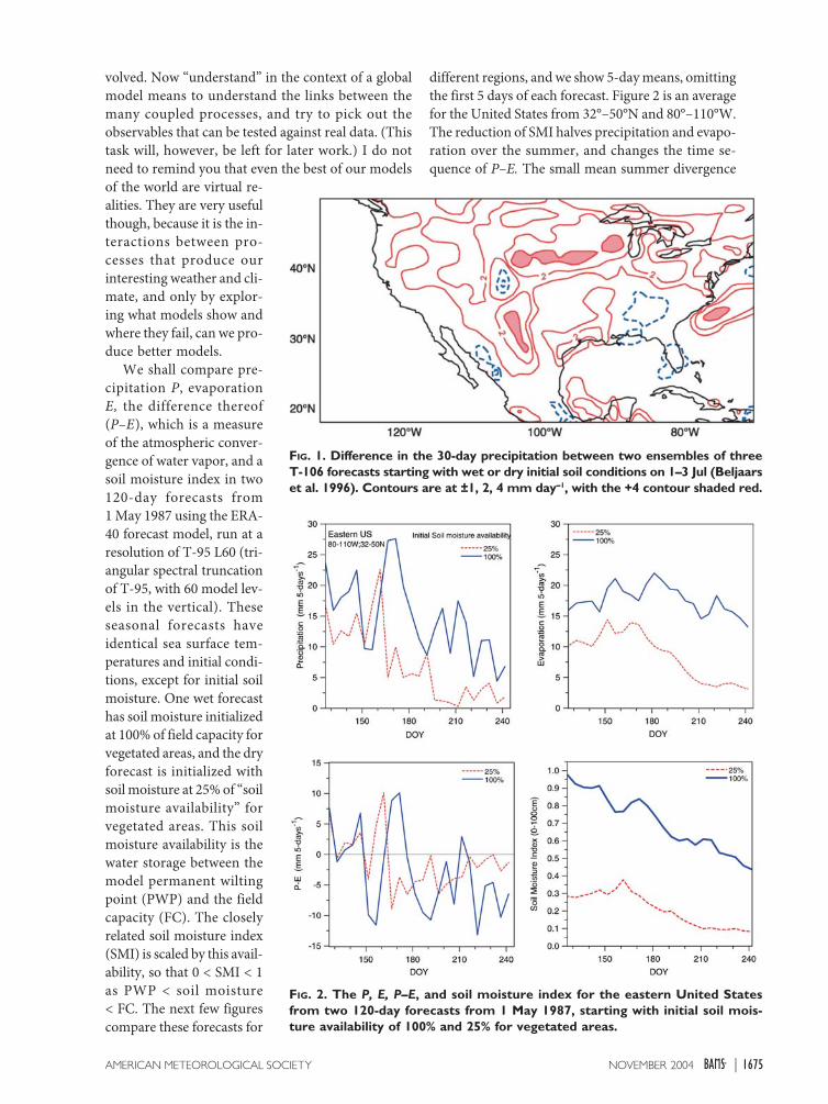
CONTINENTAL SCALE EVAPORATION–PRECIPITATION FEEDBACK: IDEALIZEDSOIL MOISTURE SIMULATIONS. The 1993Mississippi flood. This work began 10 yr ago with a littleserendipity. The great flood on the Mississippi Riverof July 1993 occurred in the same month ECMWF wasrunning in parallel its new land surface model(Viterbo and Beljaars 1995) with four soil layers tobetter represent soil moisture memory. This modelhad been developed using in part the land surface andsoil moisture data from the 1987 FIFE experiment inKansas, which I had been analyzing (Betts et al. 1993;Betts and Ball 1994, 1995). The 10-day forecasts withthe new four-soil-layer model were much better forthe July 1993 rainfall than the old two-layer model,which naturally then became history. After watchingthe catastrophic flood, I called up Martin Miller atECMWF one Friday (I think in early August) andsuggested running soil moisture sensitivity experi-ments for July 1993. We had seen considerable sensi-tivity in idealized seasonal soil moisture experiments.Forecasts starting in May with wet or dry soils showeda significant positive feedback on precipitation overthe summer. By Monday, the forecasts and diagnos-tics had been run, and Martin Miller called with someexcitement when he saw the results shown in Fig. 1.The difference in the total July precipitation betweenforecasts starting with wet or dry initial soil conditionson 1 July peaked at over 4 mm day-1 (red-shaded con-tours), corresponding to >120 mm for the month, lo-cated close to the observed precipitation maximumover the central United States. A talk on this was givenat the 1994 Nashville, Tennessee, meeting of theAmerican Meteorological Society, which was later ex-tended for publication (Beljaars et al. 1996). It is clearthat the positive feedback on precipitation is large inthe model if the soil is initially wet (we shall defineexactly how soil water was specified in a moment),and this positive signal can be seen over most of thecontinental United States. Locally, one difference wenoticed was that the cloud base was much lower overinitially wet soils.

Seasonal forecasts with idealized soil moisture. We shallnow revisit this issue globally over land with themodel used for the recent ECMWF 40-yr reanalysis(ERA-40), which has a more recent land surfacemodel, including a distribution of vegetation types(Van den Hurk et al. 2000) and other revisions to thephysics, and will try to understand the processes in-

1675NOVEMBER 2004AMERICAN METEOROLOGICAL SOCIETY |

volved. Now “understand” in the context of a globalmodel means to understand the links between themany coupled processes, and try to pick out theobservables that can be tested against real data. (Thistask will, however, be left for later work.) I do notneed to remind you that even the best of our modelsof the world are virtual re-alities. They are very usefulthough, because it is the in-teractions between pro-cesses that produce ourinteresting weather and cli-mate, and only by explor-ing what models show andwhere they fail, can we pro-duce better models.

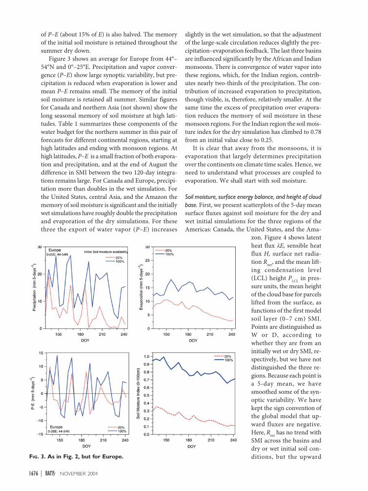
We shall compare pre-cipitation P, evaporationE, the difference thereof(P–E), which is a measureof the atmospheric conver-gence of water vapor, and asoil moisture index in two120-day forecasts from1 May 1987 using the ERA-40 forecast model, run at aresolution of T-95 L60 (tri-angular spectral truncationof T-95, with 60 model lev-els in the vertical). Theseseasonal forecasts haveidentical sea surface tem-peratures and initial condi-tions, except for initial soilmoisture. One wet forecasthas soil moisture initializedat 100% of field capacity forvegetated areas, and the dryforecast is initialized withsoil moisture at 25% of “soilmoisture availability” forvegetated areas. This soilmoisture availability is thewater storage between themodel permanent wiltingpoint (PWP) and the fieldcapacity (FC). The closelyrelated soil moisture index(SMI) is scaled by this avail-ability, so that 0 < SMI < 1as PWP < soil moisture< FC. The next few figurescompare these forecasts for

different regions, and we show 5-day means, omittingthe first 5 days of each forecast. Figure 2 is an averagefor the United States from 32°–50°N and 80°–110°W.The reduction of SMI halves precipitation and evapo-ration over the summer, and changes the time se-quence of P–E. The small mean summer divergence

FIG. 1. Difference in the 30-day precipitation between two ensembles of threeT-106 forecasts starting with wet or dry initial soil conditions on 1–3 Jul (Beljaarset al. 1996). Contours are at ±1, 2, 4 mm day-----1, with the +4 contour shaded red.

FIG. 2. The P, E, P–E, and soil moisture index for the eastern United Statesfrom two 120-day forecasts from 1 May 1987, starting with initial soil mois-ture availability of 100% and 25% for vegetated areas.

1676 NOVEMBER 2004|

of P–E (about 15% of E) is also halved. The memoryof the initial soil moisture is retained throughout thesummer dry down.

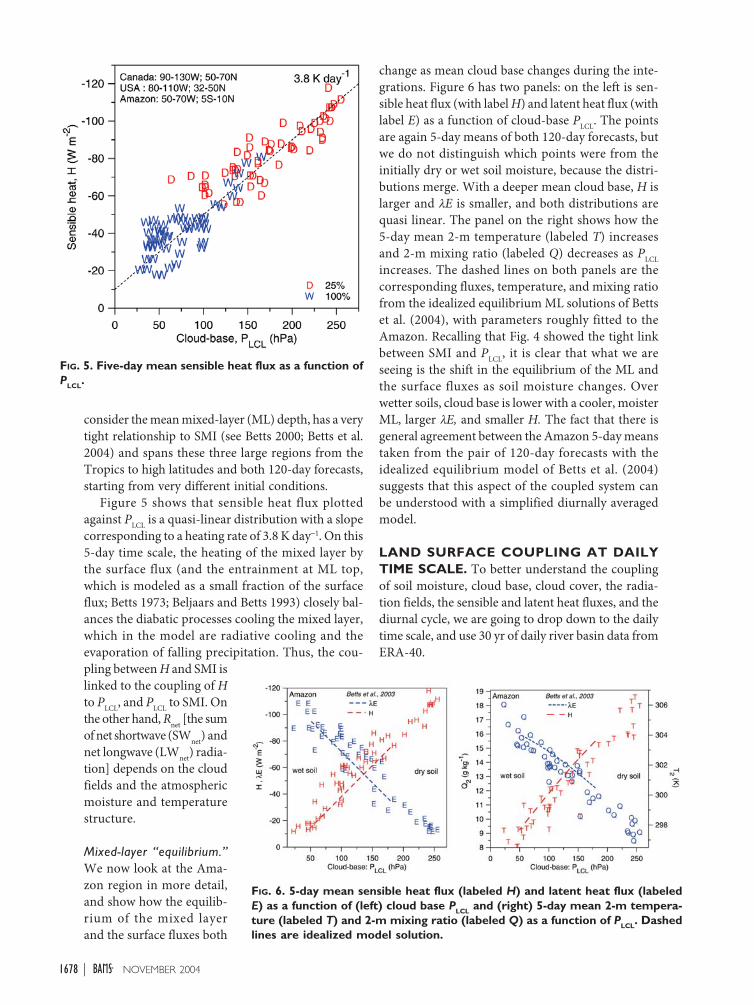
Figure 3 shows an average for Europe from 44°–54°N and 0°–25°E. Precipitation and vapor conver-gence (P–E) show large synoptic variability, but pre-cipitation is reduced when evaporation is lower andmean P–E remains small. The memory of the initialsoil moisture is retained all summer. Similar figuresfor Canada and northern Asia (not shown) show thelong seasonal memory of soil moisture at high lati-tudes. Table 1 summarizes these components of thewater budget for the northern summer in this pair offorecasts for different continental regions, starting athigh latitudes and ending with monsoon regions. Athigh latitudes, P–E is a small fraction of both evapora-tion and precipitation, and at the end of August thedifference in SMI between the two 120-day integra-tions remains large. For Canada and Europe, precipi-tation more than doubles in the wet simulation. Forthe United States, central Asia, and the Amazon thememory of soil moisture is significant and the initiallywet simulations have roughly double the precipitationand evaporation of the dry simulations. For thesethree the export of water vapor (P–E) increases

slightly in the wet simulation, so that the adjustmentof the large-scale circulation reduces slightly the pre-cipitation–evaporation feedback. The last three basinsare influenced significantly by the African and Indianmonsoons. There is convergence of water vapor intothese regions, which, for the Indian region, contrib-utes nearly two-thirds of the precipitation. The con-tribution of increased evaporation to precipitation,though visible, is, therefore, relatively smaller. At thesame time the excess of precipitation over evapora-tion reduces the memory of soil moisture in thesemonsoon regions. For the Indian region the soil mois-ture index for the dry simulation has climbed to 0.78from an initial value close to 0.25.

It is clear that away from the monsoons, it isevaporation that largely determines precipitationover the continents on climate time scales. Hence, weneed to understand what processes are coupled toevaporation. We shall start with soil moisture.

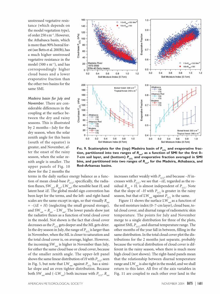
Soil moisture, surface energy balance, and height of cloudbase. First, we present scatterplots of the 5-day meansurface fluxes against soil moisture for the dry andwet initial simulations for the three regions of theAmericas: Canada, the United States, and the Ama-

zon. Figure 4 shows latentheat flux lE, sensible heatflux H, surface net radia-tion Rnet, and the mean lift-ing condensation level(LCL) height PLCL in pres-sure units, the mean heightof the cloud base for parcelslifted from the surface, asfunctions of the first modelsoil layer (0–7 cm) SMI.Points are distinguished asW or D, according towhether they are from aninitially wet or dry SMI, re-spectively, but we have notdistinguished the three re-gions. Because each point isa 5-day mean, we havesmoothed some of the syn-optic variability. We havekept the sign convention ofthe global model that up-ward fluxes are negative.Here, Rnet has no trend withSMI across the basins anddry or wet initial soil con-ditions, but the upwardFIG. 3. As in Fig. 2, but for Europe.

1677NOVEMBER 2004AMERICAN METEOROLOGICAL SOCIETY |

sensible heat decreases al-most uniformly as SMI in-creases. Latent heat flux,which can be regarded asthe sum Rnet + H (given oursign convention, and ne-glecting ground storage),does generally increase overwetter soils, but the scattercoming from the scatter inRnet is apparent. The lower-right panel shows one cru-cial link in the physics; themean depth to the cloudbase, which we can also

FIG. 4. Five-day mean latentheat flux lllllE, sensible heat fluxH, surface net radiation Rnet,and mean cloud-base heightPLCL in pressure units, as func-tions of the first model soil-layer (0–7 cm) soil moistureindex.

Canada50°–70°N, 130°–90°W 5.2 12.1 5.6 11.5 –0.4 0.6 0.19 0.86 0.67

North Asia50°–70°N, 25°–140°E 6.0 11.2 5.6 10.8 0.4 0.4 0.28 0.77 0.49

Europe44°–54°N, 0°–25°E 6.0 15.5 7.0 13.9 –1.0 1.6 0.11 0.71 0.60

United States32°–50°N, 110°–80°W 7.3 14.8 8.6 17.6 –1.3 –2.9 0.08 0.44 0.38

Central Asia35°–50°N, 40°–100°E 3.2 7.5 3.5 9.2 –0.3 –1.7 0.16 0.37 0.21

Amazon5°N–10°S, 50°–70°W 4.6 11.5 6.8 14.7 –2.2 –3.2 0.04 0.27 0.23

Equatorial Africa10°N–10°S, 14°–35°E 12.6 18.5 8.9 13.3 3.7 5.2 0.40 0.62 0.22

Africa/Sahel10°–20°N, 15°W–40°E 14.8 18.2 7.1 10.0 7.6 8.1 0.58 0.67 0.09

India18°–35°N, 70°–90°E 28.4 32.7 9.3 14.3 19.1 18.4 0.78 0.93 0.15

TABLE 1. Five-day mean summer precipitation P, evaporation E, P–E, and end-of-Aug soil moisture indexfor forecasts with initial dry and wet soil moisture index.

Precipitation Evaporation P–E SMI (0–100 cm) Diff(mm 5-day-----1) (mm 5-day-----1) (mm 5-day-----1) day = 241.5 of SMI

Initial SMI: Dry Wet Dry Wet Dry Wet Dry Wet

1678 NOVEMBER 2004|

consider the mean mixed-layer (ML) depth, has a verytight relationship to SMI (see Betts 2000; Betts et al.2004) and spans these three large regions from theTropics to high latitudes and both 120-day forecasts,starting from very different initial conditions.

Figure 5 shows that sensible heat flux plottedagainst PLCL is a quasi-linear distribution with a slopecorresponding to a heating rate of 3.8 K day-1. On this5-day time scale, the heating of the mixed layer bythe surface flux (and the entrainment at ML top,which is modeled as a small fraction of the surfaceflux; Betts 1973; Beljaars and Betts 1993) closely bal-ances the diabatic processes cooling the mixed layer,which in the model are radiative cooling and theevaporation of falling precipitation. Thus, the cou-pling between H and SMI islinked to the coupling of Hto PLCL, and PLCL to SMI. Onthe other hand, Rnet [the sumof net shortwave (SWnet) andnet longwave (LWnet) radia-tion] depends on the cloudfields and the atmosphericmoisture and temperaturestructure.

Mixed-layer “equilibrium.”We now look at the Ama-zon region in more detail,and show how the equilib-rium of the mixed layerand the surface fluxes both

change as mean cloud base changes during the inte-grations. Figure 6 has two panels: on the left is sen-sible heat flux (with label H) and latent heat flux (withlabel E) as a function of cloud-base PLCL. The pointsare again 5-day means of both 120-day forecasts, butwe do not distinguish which points were from theinitially dry or wet soil moisture, because the distri-butions merge. With a deeper mean cloud base, H islarger and lE is smaller, and both distributions arequasi linear. The panel on the right shows how the5-day mean 2-m temperature (labeled T) increasesand 2-m mixing ratio (labeled Q) decreases as PLCLincreases. The dashed lines on both panels are thecorresponding fluxes, temperature, and mixing ratiofrom the idealized equilibrium ML solutions of Bettset al. (2004), with parameters roughly fitted to theAmazon. Recalling that Fig. 4 showed the tight linkbetween SMI and PLCL, it is clear that what we areseeing is the shift in the equilibrium of the ML andthe surface fluxes as soil moisture changes. Overwetter soils, cloud base is lower with a cooler, moisterML, larger lE, and smaller H. The fact that there isgeneral agreement between the Amazon 5-day meanstaken from the pair of 120-day forecasts with theidealized equilibrium model of Betts et al. (2004)suggests that this aspect of the coupled system canbe understood with a simplified diurnally averagedmodel.

LAND SURFACE COUPLING AT DAILYTIME SCALE. To better understand the couplingof soil moisture, cloud base, cloud cover, the radia-tion fields, the sensible and latent heat fluxes, and thediurnal cycle, we are going to drop down to the dailytime scale, and use 30 yr of daily river basin data fromERA-40.

FIG. 5. Five-day mean sensible heat flux as a function ofPLCL.

FIG. 6. 5-day mean sensible heat flux (labeled H) and latent heat flux (labeledE) as a function of (left) cloud base PLCL and (right) 5-day mean 2-m tempera-ture (labeled T) and 2-m mixing ratio (labeled Q) as a function of PLCL. Dashedlines are idealized model solution.

1679NOVEMBER 2004AMERICAN METEOROLOGICAL SOCIETY |

ERA-40 river basin budgets. The research archive fromERA-40 contains an hourly time series, averaged overselected river basins (with the fluxes integrated fromthe full time resolution of the model). These have beenused to assess the biases of ERA-40 at the surface againstdata from the Mackenzie and Mississippi River basins(Betts et al. 2003a,b). Figure 7 shows these basins forthe Americas: the red-numbered quadrilaterals are themodel approximation to the river basins shown inbrown (the blue numbers correspond to archive pointswhere there are flux tower observations for compari-son). For this paper, we choose three river subbasins:

• 42: Madeira: a southwestern subbasin of theAmazon,

• 28: Arkansas–Red: a southwestern subbasin of theMississippi, and

• 39: Athabasca: a southeastern subbasin of theMackenzie.

From the hourly time series, we computed daily av-erages for the 30-yr period from January 1972 to May2002, some 11,000 days, as well as the diurnal rangeof temperature and relative humidity. In addition tothe basic state variables and fluxes, we also have themodel cloud cover.

Diurnal and seasonal cycles of ERA-40 for Madeira Riverbasin compared with LBA Rondonia pasture site for 1999.First we compare in Fig. 8 the diurnal and seasonalcycles of ERA-40 for the Madeira River basin with theLBA pasture site in Rondonia, Brazil (see Betts et al.2002), within this basin. Comparing the Rondoniapoint data and the ERA-40 Madeira basin mean ishardly a fair comparison, but we see broadly similardiurnal and seasonal structure, with the much larger-scale basin mean having a reduced seasonal range. Thefour panels for the Madeira basin and Rondonia pas-ture, respectively, in Fig. 8 show the mean diurnalcycle of near-surface temperature, mixing ratio,equivalent potential temperature, and PLCL, the pres-sure height to the LCL. The colors from blue to redshow the transition in the mean diurnal cycle fromthe rainy season through to the dry season in August,averaged for the months shown. Note that the meantemperature changes little, but the amplitude of thediurnal cycle of temperature increases sharply fromthe rainy to the dry season as the outgoing LWnet in-creases (not shown). This is associated with the drier(and less cloudy) atmosphere. The mean LCL heightPLCL (a good approximation to mean cloud base in thedaytime) grows from the rainy to dry season, and theML gets warmer and drier.

Coupling of soil moisture index, cloud-base height, andevaporative fraction. These daily mean data from ERA-40 from 1972 to 2002 can be used to explore the link

FIG. 7. ERA-40 basin and point hourly archive for theAmericas. The red-numbered quadrilaterals are themodel approximations to the river basins shown inbrown; the blue numbers correspond to archive points,where there are flux tower observations for comparison.

1680 NOVEMBER 2004|

between soil moisture,cloud-base height, andevaporative fraction [de-fined as lE/(lE + H)]. Theupper panels of Fig. 9 forthe Madeira basin are PLCLand evaporative fraction asa function of SMI for thefirst 0–7-cm soil layer, par-titioned into two ranges ofRnet, 110 < Rnet < 150 W m-2

and 150 < Rnet < 190 W m-2.We see that the meancloud-base height increasesover drier soils and withlarger surface Rnet, whileevaporative fraction in-creases with soil moisture,and decreases with Rnet.The lower panels of Fig. 9average the daily pointsinto 0.1 range bins of SMI,and add the summer data[June–July–August (JJA)]for the Arkansas–Red andAthabasca basins. Againwe have split the data intothe same two ranges of Rnetand labeled the curves withthe midrange values of 130and 170 W m-2; in addi-tion, we have added thestandard deviation for thelower Rnet range to showhow tight the distributionsare. Within the error bars,the Arkansas–Red and Ma-deira basins form a singledistribution, even thoughsoil moisture is muchlower in the Arkansas–Redbasin. The tropical forestand this southern basin ofthe Mississippi have similar

a)

b)

FIG. 8. Comparison of the sea-sonal change of the mean di-urnal cycle of near-surfacetemperature, mixing ratio,equivalent potential tempera-ture, and PLCL for ERA-40 forthe Madeira River basin, withthe LBA pasture site inRondonia.

1681NOVEMBER 2004AMERICAN METEOROLOGICAL SOCIETY |

unstressed vegetative resis-tance (which depends onthe model vegetation type),of order 250 s m-1. However,the Athabasca basin, whichis more than 90% boreal for-est (see Betts et al. 2003b), hasa much higher unstressedvegetative resistance in themodel (500 s m-1), and hascorrespondingly highercloud bases and a lowerevaporative fraction thanthe other two basins for thesame SMI.

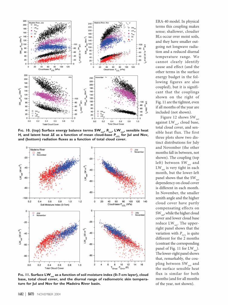
Madeira basin for July andNovember. There are con-siderable differences in thecoupling at the surface be-tween the dry and rainyseasons. This is illustratedby 2 months—July for thedry season, when the solarzenith angle for this basin(south of the equator) isgreater, and November, af-ter the onset of the rainyseason, when the solar ze-nith angle is smaller. Theupper panels of Fig. 10show for the 2 months theterms in the daily surface energy balance as a func-tion of mean cloud-base PLCL, specifically, the radia-tion fluxes, SWnet, Rnet, LWnet, the sensible heat H, andlatent heat lE. The global model sign convention hasbeen kept for the terms, and the left- and right-handscales are the same except in sign, so that visually Rnet= –(lE + H) (neglecting the small ground storage),and SWnet = Rnet – LWnet. The lower panels show justthe radiative fluxes as a function of total cloud coverin the model. Not shown is the fact that cloud coverdecreases as the PLCL gets deeper and the ML gets drier.In the dry season in July, the range of PLCL is larger thanin November, when the ML is closer to saturation andthe total cloud cover is, on average, higher. However,the incoming SWnet is higher in November than July,for either the same cloud base or cloud cover, becauseof the smaller zenith angle. The upper-left panelshows the same linear distribution of H with PLCL, seenin Fig. 5, but note that LWnet against PLCL has a simi-lar slope and an even tighter distribution. Becauseboth SWnet and (–LWnet) both increase with PLCL, Rnet

increases rather weakly with PLCL, and because –H in-creases with PLCL, we see that –lE, regarded as the re-sidual Rnet + H, is almost independent of PLCL. Notethat the slope of –H with PLCL is greater in the rainyseason, but that of LWnet against PLCL is the same.

Figure 11 shows the surface LWnet as a function ofthe soil moisture index (0–7-cm layer), cloud base, to-tal cloud cover, and diurnal range of radiometric skintemperature. The points for July and Novembermerge to a single distribution for three of the plots,against SMI, PLCL, and diurnal temperature range. Theother months of the year fall in between, filling in thesame distribution. In the total cloud cover plot the dis-tributions for the 2 months just separate, probablybecause the vertical distribution of cloud cover is dif-ferent in the rainy season, when there is much morehigh cloud (not shown). The right-hand panels meanthat the relationship between diurnal temperaturerange and LWnet is also tight in the model, and we shallreturn to this later. All five of the axis variables inFig. 11 are coupled to each other over land in the

FIG. 9. Scatterplots for the (top) Madeira basin of PLCL and evaporative frac-tion, partitioned into two ranges of Rnet, as a function of SMI for the first 0–7-cm soil layer, and (bottom) PLCL and evaporative fraction averaged in SMIbins, and partitioned into two ranges of Rnet, for the Madeira, Athabasca, andRed–Arkansas basins.

1682 NOVEMBER 2004|

ERA-40 model. In physicalterms this coupling makessense; shallower, cloudierBLs occur over moist soils,and they have smaller out-going net longwave radia-tion and a reduced diurnaltemperature range. Wecannot clearly identifycause and effect (and theother terms in the surfaceenergy budget in the fol-lowing figures are alsocoupled), but it is signifi-cant that the couplingsshown on the right ofFig. 11 are the tightest, evenif all months of the year areincluded (not shown).

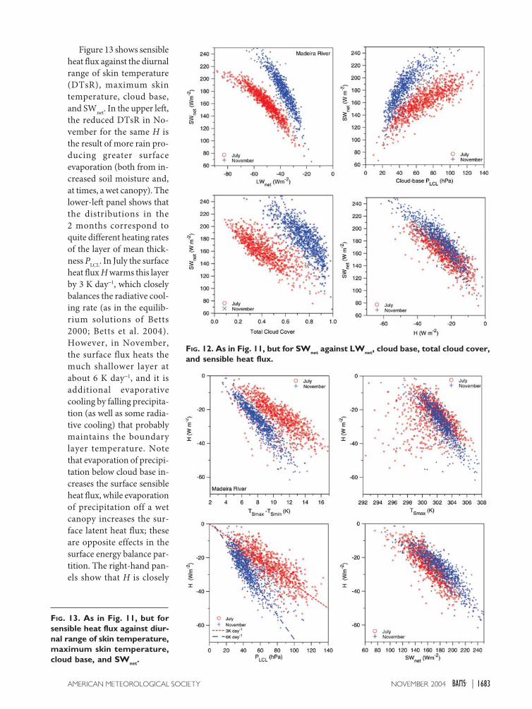
Figure 12 shows SWnetagainst LWnet, cloud base,total cloud cover, and sen-sible heat flux. The firstthree plots show two dis-tinct distributions for Julyand November (the othermonths fall in between, notshown). The coupling (topleft) between SWnet andLWnet is very tight in eachmonth, but the lower-leftpanel shows that the SWnetdependency on cloud coveris different in each month.In November, the smallerzenith angle and the highercloud cover have partlycompensating effects onSWnet, while the higher cloudcover and lower cloud basereduce LWnet. The upper-right panel shows that thevariation with PLCL is quitedifferent for the 2 months(contrast the correspondingpanel of Fig. 11 for LWnet).The lower-right panel showsthat, remarkably, the cou-pling between SWnet andthe surface sensible heatflux is similar for bothmonths (and for all monthsof the year, not shown).

FIG. 10. (top) Surface energy balance terms SWnet, Rnet, LWnet, sensible heatH, and latent heat lllllE as a function of mean cloud-base PLCL for Jul and Nov,and (bottom) radiation fluxes as a function of total cloud cover.

FIG. 11. Surface LWnet as a function of soil moisture index (0–7-cm layer), cloudbase, total cloud cover, and the diurnal range of radiometric skin tempera-ture for Jul and Nov for the Madeira River basin.

1683NOVEMBER 2004AMERICAN METEOROLOGICAL SOCIETY |

Figure 13 shows sensibleheat flux against the diurnalrange of skin temperature(DTsR), maximum skintemperature, cloud base,and SWnet. In the upper left,the reduced DTsR in No-vember for the same H isthe result of more rain pro-ducing greater surfaceevaporation (both from in-creased soil moisture and,at times, a wet canopy). Thelower-left panel shows thatthe distributions in the2 months correspond toquite different heating ratesof the layer of mean thick-ness PLCL. In July the surfaceheat flux H warms this layerby 3 K day-1, which closelybalances the radiative cool-ing rate (as in the equilib-rium solutions of Betts2000; Betts et al. 2004).However, in November,the surface flux heats themuch shallower layer atabout 6 K day-1, and it isadditional evaporativecooling by falling precipita-tion (as well as some radia-tive cooling) that probablymaintains the boundarylayer temperature. Notethat evaporation of precipi-tation below cloud base in-creases the surface sensibleheat flux, while evaporationof precipitation off a wetcanopy increases the sur-face latent heat flux; theseare opposite effects in thesurface energy balance par-tition. The right-hand pan-els show that H is closely

FIG. 12. As in Fig. 11, but for SWnet against LWnet, cloud base, total cloud cover,and sensible heat flux.

FIG. 13. As in Fig. 11, but forsensible heat flux against diur-nal range of skin temperature,maximum skin temperature,cloud base, and SWnet.

1684 NOVEMBER 2004|

coupled to the maximum skin temperature (upperright), and we repeat the coupling to SWnet. The skintemperature responds to the daytime shortwave (SW)radiation, and H to the skin temperature. We see thatH is coupled to several processes—the SW forcing atthe surface, and the radiative and evaporative cool-ing of the layer below mean cloud base—and all ofthese processes are coupled to the cloud fields.

Figure 14 shows latent heat flux lE and sensibleheat flux H against the soil moisture index (top) andRnet (bottom). It is the sensible heat flux (top right)rather than the evaporation (top left) that can be seento vary with SMI (but the variation differs for the2 months). SMI controls PLCL quite directly (seeFig. 9), but in the rainy season H is increased by ad-ditional BL cooling processes (Fig. 13). The lowerpanels show the links between the fluxes and Rnet.Latent heat lE has more variation with Rnet in Novem-ber, representative of the rainy season months fromNovember to April, while July is representative of themuch weaker variation of lE with Rnet in the dry sea-son. Contrast (lower right) the two branches for H asa function of Rnet with the corresponding lower-rightpanel of the previous Fig. 13 against SWnet.

Priestley–Taylor ratio. Figures 10–14 explore the inter-relationship on the daily time scale between many pa-rameters: the surface sensible and latent heat fluxes,soil moisture index, total cloud cover, height of cloudbase, and net shortwave and longwave fluxes. Whatdo these relationships mean for evaporation in termsof the classic Priestley–Taylor ratio, which may be de-fined as

Priestley–Taylor ratio = EF(1+e)/e, (1)

where EF = lE/(Rnet – G) = lE/(lE + H)? The ther-modynamic coefficient e = (l/Cp)dQs/dT is related tothe change of saturation mixing ratio with tempera-ture (following Betts 1994, we define this at the LCLtemperature).

Figure 15 shows the scatterplot of the Priestley–Taylor ratio for July and November for the Madeirabasin against SMI and Rnet. We see the now-familiartwo separate branches for July and November. Bothshow higher values of the Priestley–Taylor ratio forhigher soil water and lower Rnet, with upper valuesnear 1.26, consistent with many previous analyses.The 20% variation in the Priestley–Taylor ratio

corresponds to a 20 W m-2

change in the partition ofthe surface energy budget.While an error of 10%–20% might be acceptable insurface evaporation forsome more traditional hy-drological purposes, for cli-mate interactions overlandthis is a large error. Thismeans that we must bothunderstand the couplingwith the cloud field and BLstructure shown in figures10–14, and also validate therelationships shown in themodel against observations.

LW coupling for other basins.The coupling of the LWnet tototal cloud cover and PLCL,shown in Fig. 11, is quitegeneral. Figure 16 showsfor the three Americas’ ba-sins the mean variation ofLWnet against total cloudcover, binned in 0.2 binranges, and against cloud-base PLCL (in 20-hPa bins).

FIG. 14. As in Fig. 11, but for latent heat flux lllllE and sensible heat flux H against(top) soil moisture index and (bottom) Rnet.

1685NOVEMBER 2004AMERICAN METEOROLOGICAL SOCIETY |

The Madeira basin dailydata covers the full 30 yr,while the Athabasca andRed–Arkansas basin dataare for summer (JJA) only.In the left-hand plotagainst total cloud cover,the curve for the Madeirabasin is above the mid-latitude basins, but this isconsistent with it having a50-hPa mean lower cloudbase, and a moister BL. Onthe right, the Red–Arkansasis below the other two, butthis too is consistent with ithaving a lower total cloudcover (about 0.25 less thanthe Athabasca). There is aonly a small shift of the dis-tribution, for the same PLCLand cloud cover, to largeroutgoing LW at high lati-tudes as the emissivity ofthe overlying atmospheredecreases. This tight cou-pling between LWnet andPLCL is undoubtedly an im-portant land surface feed-back, as noted by Schäret al. (1999). Over wet soils,the cloud base is lower andthe outgoing longwave ra-diation is decreased.

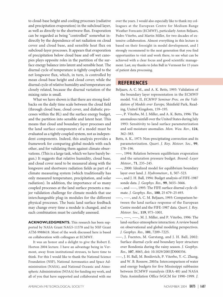
Diurnal cycle. The last part of this analysis addressesthe diurnal cycle of temperature and relative humid-ity (RH), both important aspects of the climatesystem. Figure 17 for the Madeira basin showsmaximum and minimum skin temperatures TSmaxand TSmin, respectively, and the difference DTsR(right-hand scale) plotted against LWnet. Note thatDTsR is coupled quite tightly to LWnet, as shownpreviously in Fig. 11; the width of the distribution isless than that of either TSmax or TSmin. Figure 18 (leftpanel) plots the diurnal range of the 2-m tempera-ture (DT2R), an important climate variable, againstLWnet. Also plotted is the temperature changecomputed from LWnet and the slope of the Planckfunction

DTPlanck = –LWnet/4sT3. (2)

FIG. 15. Priestley–Taylor ratio for Jul and Nov for the Madeira basin plottedagainst soil moisture index and Rnet.

FIG. 16. Mean variation of LWnet against total cloud cover and cloud-base PLCL

for the three Americas basins.

FIG. 17. Maximum and minimum skin temperaturesTSmax and TSmin, respectively, and the diurnal range ofskin temperature (right-hand scale) plotted againstLWnet for the Madeira basin.

1686 NOVEMBER 2004|

Not only is diurnal range of temperature tightly re-lated to the LWnet, but DTPlanck gives a good estimateof DT2R in the model in the Tropics. At higher lati-tudes, the ratio DT2R/DTPlanck decreases to 0.8 (notshown). The right panel of Fig. 18 shows the tight cou-pling between the diurnal temperature range and thediurnal range of RH (scaled by the diurnal mean ofRH). This is largely a result of the fact that the diur-nal range of mixing ratio Q is small (see Fig. 8), be-cause the large surface evaporation is transported upthrough the cloud base. The dotted line is the couplingfor constant Q. Except for large values of DT2R, whichcorrespond to deep, dry daytime BLs, the points forthe Madeira basin lie below the dotted line, becauseat the temperature minimum, the surface air saturatesand Qs(Tmin) is less than Q(Tmax). Drier basins, suchas the Red–Arkansas (not shown), show a small up-ward shift of the distribution relative to the dashedconstant Q line.

CONCLUSIONS. Modeling climate and climatechange over land depends critically on the couplingbetween the cloud and radiation fields, the surfacepartition of sensible and latent heat, soil water (andother constraints on evaporative resistance), and theboundary layer (as well as subsurface hydrologic pro-cesses that we have not addressed here); so we havetried to map out some of these links in the ECMWFmodel at the time of ERA-40. The first section ad-dressed evaporation–precipitation feedback in sea-sonal forecasts for the Northern Hemisphere summer,initialized with idealized “wet” and “dry” soils forvegetated areas. We showed that away from the mon-soon regions, the ERA-40 model has a large evapora-tion–precipitation feedback over the continents, and

the memory of initial soilmoisture is longest at highnorthern latitudes. Wemight well ask whether thisstrong feedback is correct,because other work (Kosteret al. 2002) shows that thisfeedback differs widely indifferent models, presum-ably because each modeldiffers in the way it param-eterizes the many physicalprocesses we have dis-cussed. We then showedthat the change in the sur-face energy budget over dryand wet soils is consistentwith a shift of the mean

subcloud-layer equilibrium, and is also broadly con-sistent with an idealized (diurnally averaged) equilib-rium model for the boundary layer.

The second section addressed the coupling of thesoil moisture, cloud base, cloud cover, radiation fields,sensible and latent heat fluxes, and diurnal cycle, us-ing 30 yr of daily river basin data from ERA-40 for threebasins in the Americas: the Madeira, Red–Arkansas,and Athabasca. It is clear that the tight coupling tocloud processes plays an essential role in the BL equi-librium, and that although the model fully resolves thediurnal cycle and has a prognostic interactive cloudfield, the transitions in the BL climate over land cannonetheless be mapped with remarkable precision bythe daily mean state and daily flux averages.

Mean cloud-base height increases over drier soilswith larger surface Rnet, while evaporative fraction in-creases with soil moisture and decreases with Rnet. Thedifferences in the coupling at the surface between thedry season and the rainy season were illustrated forthe Madeira basin by selecting 2 months: July for thedry season, and November, after the onset of the rainyseason. Both surface LWnet and H have similar linearslopes when plotted against PLCL in the dry season,with LWnet having a rather tighter distribution. Moregenerally, it is clear that model data such as that fromERA-40 can be used to understand the coupling ofprocesses at the land surface. Soil moisture, cloudbase, cloud cover, radiation fields, and evaporativefraction are indeed coupled quite tightly on daily av-erage time scales. The longwave flux control by cloud-base height and cloud cover is particularly tight acrossall basins, and is, thus, an important feedback betweenthe cloud field and the surface energy budget, as notedby Schär et al. (1999). The sensible heat flux is coupled

FIG. 18. Diurnal range of the 2-m temperature DDDDDTPlanck [see Eq. (2)] plottedagainst (left) LWnet and (right) the coupling between the diurnal range of RH,scaled by the diurnal mean of RH, and the diurnal temperature range for theMadeira basin.

1687NOVEMBER 2004AMERICAN METEOROLOGICAL SOCIETY |

to cloud-base height and cooling processes (radiativeand precipitation evaporation) in the subcloud layer,as well as directly to the shortwave flux. Evaporationcan be regarded as being “controlled” somewhat in-directly by the dependence of net radiation on cloudcover and cloud base, and sensible heat flux onsubcloud-layer processes. It appears that evaporationof precipitation below cloud base and off wet cano-pies plays opposite roles in the partition of the sur-face energy balance into latent and sensible heat. Thediurnal cycle of temperature is tightly coupled to thenet longwave flux, which, in turn, is controlled bymean cloud-base height and cloud cover; while thediurnal cycle of relative humidity and temperature areclosely related, because the diurnal variation of themixing ratio is small.

What we have shown is that there are strong feed-backs on the daily time scale between the cloud field(through cloud base, cloud cover, and diabatic pro-cesses within the BL) and the surface energy budget,and the partition into sensible and latent heat. Thismeans that cloud and boundary layer processes andthe land surface components of a model must beevaluated as a tightly coupled system, not as indepen-dent components. Indeed, this analysis provides aframework for comparing global models with eachother, and for validating them against climate obser-vations. (This is a large task, which we have barely be-gun.) It suggests that relative humidity, cloud base,and cloud cover need to be measured along with thelongwave and shortwave radiation fields as part of aclimate measuring system (which traditionally hasonly measured temperature, precipitation, and solarradiation). In addition, the importance of so manycoupled processes at the land surface presents a ma-jor validation challenge for climate models that useinterchangeable plug-in modules for the differentphysical processes. The basic land surface feedbackmay change every time a module is changed, and soeach combination must be carefully assessed.

ACKNOWLEDGMENTS. This research has been sup-ported by NASA Grant NAG5-11578 and by NSF GrantATM-9988618. Most of the work discussed here is basedon collaboration with colleagues at ECMWF.

It was an honor and a delight to give the Robert E.Horton 2004 lecture. I have an advantage being in Ver-mont, away from institutional stresses, to have time tothink. For this I would like to thank the National ScienceFoundation (NSF), National Aeronautics and Space Ad-ministration (NASA), and National Oceanic and Atmo-spheric Administration (NOAA) for funding my work, andall of you that have supported and collaborated with me

over the years. I would also especially like to thank my col-leagues at the European Centre for Medium-RangeWeather Forecasts (ECMWF), particularly Anton Beljaars,Pedro Viterbo, and Martin Miller, for two decades of ex-tensive collaboration. Almost everything in this lecture isbased on their foresight in model development, and Istrongly recommend to the next generation that you findopportunities to visit and work there, to see what can beachieved with a clear focus and good scientific manage-ment. Last, my thanks to John Ball in Vermont for 15 yearsof patient data processing.

REFERENCESBeljaars, A. C. M., and A. K. Betts, 1993: Validation of

the boundary layer representation in the ECMWFmodel. Vol. II, ECMWF Seminar Proc. on the Vali-dation of Models over Europe, Shinfield Park, Read-ing, United Kingdom, 159–195.

——, P. Viterbo, M. J. Miller, and A. K. Betts, 1996: Theanomalous rainfall over the United States during July1993: Sensitivity to land surface parameterizationand soil moisture anomalies. Mon. Wea. Rev., 124,362–383.

Betts, A. K., 1973: Non-precipitating convection and itsparameterization. Quart. J. Roy. Meteor. Soc., 99,178–196.

——, 1994: Relation between equilibrium evaporationand the saturation pressure budget. Bound.-LayerMeteor., 71, 235–245.

——, 2000: Idealized model for equilibrium boundarylayer over land. J. Hydrometeor., 1, 507–523.

——, and J. H. Ball, 1994: Budget analysis of FIFE-1987sonde data. J. Geophys. Res., 99, 3655–3666.

——, and ——, 1995: The FIFE surface diurnal cycle cli-mate. J. Geophys. Res., 100, 25 679–25 693.

——, ——, and A. C. M. Beljaars, 1993: Comparison be-tween the land surface response of the EuropeanCentre model and the FIFE-1987 data. Quart. J. Roy.Meteor. Soc., 119, 975–1001.

——, ——, ——, M. J. Miller, and P. Viterbo, 1996: Theland-surface-atmosphere interaction: A review basedon observational and global modeling perspectives.J. Geophys. Res., 101, 7209–7225.

——, J. Fuentes, M. Garstang, and J. H. Ball, 2002:Surface diurnal cycle and boundary layer structureover Rondonia during the rainy season. J. Geophys.Res., 107, 8065, doi: 10.1029/2001JD000356.

——, J. H. Ball, M. Bosilovich, P. Viterbo, Y.-C. Zhang,and W. B. Rossow, 2003a: Intercomparison of waterand energy budgets for five Mississippi subbasinsbetween ECMWF reanalysis (ERA-40) and NASAData Assimilation Office fvGCM for 1990–1999. J.

1688 NOVEMBER 2004|

Geophys. Res., 108 (D16), 8618, doi:10.1029/2002JD003127.

——, ——, and P. Viterbo, 2003b: Evaluation of the ERA-40 surface water budget and surface temperature forthe Mackenzie River basin. J. Hydrometeor., 4, 1194–1211.

——, B. Helliker, and J. Berry, 2004: Coupling betweenCO2, water vapor, temperature and radon and theirfluxes in an idealized equilibrium boundary layerover land. J. Geophys. Res., 109 (D18103),doi:10.1029/2003JD004420.

Koster, R. D., P. A. Dirmeyer, A. N. Hahmann,R. Ijpelaar, L. Tyahla, P. Cox, and M. J. Suarez, 2002:Comparing the degree of land–atmosphere interac-tion in four atmospheric general circulation models.J. Hydrometeor., 3, 363–375.

Raupach, M., 2000: Equilibrium evaporation and theconvective boundary layer. Bound.-Layer Meteor., 96,107–141.

——, 2001: Combination theory and equilibriumevaporation. Quart. J. Roy. Meteor. Soc., 127, 1149–1181.

Schär, C., D. Lüthi, U. Beyerle, and E. Heise, 1999: Thesoil–precipitation feedback: A process study with aregional climate model. J. Climate, 12, 722–741.

Van den Hurk, B. J. J. M., P. Viterbo, A. C. M. Beljaars,and A. K. Betts, 2000: Offline validation of the ERA40surface scheme. ECMWF Tech. Memo. 295, 43 pp.[Available online at www.ecmwf.int/publications/library/ecpublications/_pdf/tm/001-300/tm295.pdf.]

Viterbo, P., and A. C. M. Beljaars, 1995: An improvedland surface parameterization in the ECMWF modeland its validation. J. Climate, 8, 2716–2748.