ABSTRACTThe IEC-60870-5-104 (IEC-104) protocol is commonly used in Super-visory Control and Data Acquisition (SCADA) networks to operatecritical infrastructures, such as power stations. As the importanceof SCADA security is growing, characterization and modeling ofSCADA traffic for developing defense mechanisms based on theregularity of the polling mechanism used in SCADA systems hasbeen studied, whereas the characterization of traffic caused by non-polling mechanisms, such as spontaneous events, has not beenwell-studied. This paper provides a first look at how the traffic flow-ing between SCADA components changes over time. It proposes amethod built upon Probabilistic Suffix Tree (PST) to discover theunderlying timing patterns of spontaneous events. In 11 out of 14tested data sequences, we see evidence of existence of underlyingpatterns. Next, the prediction capability of the approach, useful fordevising anomaly detection mechanisms, is studied. While somedata patterns enable an 80% prediction possibility, more work isneeded to tune the method for higher accuracy.
ACM Reference Format:Chih-Yuan Lin and Simin Nadjm-Tehrani. 2018. Understanding IEC-60870-5-104 Traffic Patterns in SCADA Networks. In CPSS’18: The 4th ACM Cyber-Physical System Security Workshop, June 4, 2018, Incheon, Republic of Korea.ACM,NewYork, NY, USA, 10 pages. https://doi.org/10.1145/3198458.3198460
1 INTRODUCTIONModern Supervisory Control and Data Acquisition (SCADA) sys-tems increasingly depend on information and communication tech-nologies and become connected to the Internet to allow greater
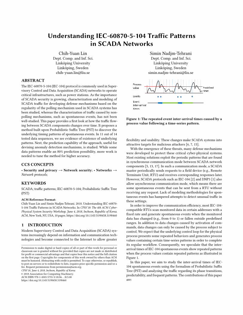
Figure 1: The repeated event inter-arrival times caused by aprocess value following a time-series pattern.
flexibility and usability. These changes make SCADA systems intoattractive targets for malicious attackers [6, 7, 15].
With the emergence of these threats, many defense mechanismswere developed to protect these critical cyber-physical systems.Most existing solutions exploit the periodic patterns that are foundin synchronous communication mode between SCADA networkcomponents [5, 13, 17]. In such a communication mode, a SCADAmaster periodically sends requests to a field device (e.g., RemoteTerminate Unit, RTU) and receives corresponding responses later.However, SCADA protocols such as IEC-104 [2] and DNP3 [1] alsoallow asynchronous communication mode, which means there aresome spontaneous events that can be sent from a RTU withoutreceiving any request. Lack of modeling methodologies for spon-taneous events has hampered attempts to detect unusual traffic inthese settings.
In order to improve the communication efficiency, most IEC-104-compatible RTUs scan monitored data in certain addresses with afixed rate and generate spontaneous events when the monitoreddata has changed (e.g., from 0 to 1) or fallen outside predefinedranges. In addition to data changes caused by activation of com-mands, data changes can only be caused by the process subject tocontrol. We expect that the underlying control loop for the physicalprocess presents some repeated behaviors and generates processvalues containing certain time-series patterns in order to completeits regular workflow. Consequently, we speculate that the inter-arrival times of IEC-104 spontaneous events show repeated patternswhen the process values contain repeated patterns as illustrated inFigure 1.
In this paper, we aim to study the inter-arrival times of IEC-104 spontaneous events using the formalism of Probabilistic SuffixTree (PST) and analyzing the traffic regarding its phase transitions,predictability, and frequent patterns. The contributions of this paperare:
CPSS’18, June 4, 2018, Incheon, Republic of Korea Chih-Yuan Lin and Simin Nadjm-Tehrani
• We provide a systematic approach to model the timing ofIEC-104 spontaneous traffic generated from a RTU and aprocess that follows the above hypothesis.• Using data from emulated traffic in test labs, we show thatthere exists certain timing patterns in the IEC-104 sponta-neous traffic and the patterns could provide prediction abilityover a long observation time.
The rest of the paper is organized as follows. Section 2 providesthe needed background about IEC-104 and PST. Section 3 discussesthe related work. Section 4 describes the proposed modeling ap-proach. Section 5 provides the overview of datasets used in thispaper and presents the analysis of traffic. Finally, Section 6 con-cludes the paper and describes the future works.
2 BACKGROUNDThis section provides an overview of IEC-104 protocol and theframe format used in this study. It also presents a brief introductionof PST with a focus of calculation of conditional and zero-orderprobabilities, which are used in our analysis.
2.1 IEC-60870-5-104The IEC-104 protocol is widely used in modern SCADA systems.The basic frame in the IEC-104 protocol is called Application Pro-tocol Data Unit (APDU) and an APDU frame can be in U, S or Iformat. The unnumbered control frame (U) is used for test, startor stop communication flows. The supervisory format (S) is usedto perform numbered supervisory functions. The information in-struction format (I) is used for sending numbered commands andinformation. Spontaneous events can only be sent in the I format.
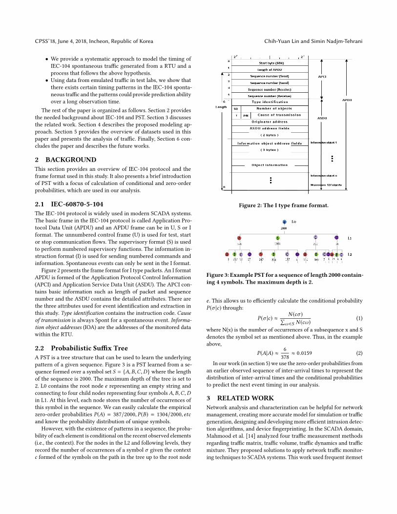
Figure 2 presents the frame format for I type packets. An I formatAPDU is formed of the Application Protocol Control Information(APCI) and Application Service Data Unit (ASDU). The APCI con-tains basic information such as length of packet and sequencenumber and the ASDU contains the detailed attributes. There arethe three attributes used for event identification and extraction inthis study. Type identification contains the instruction code. Causeof transmission is always Spont for a spontaneous event. Informa-tion object addresses (IOA) are the addresses of the monitored datawithin the RTU.
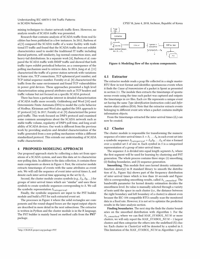
2.2 Probabilistic Suffix TreeA PST is a tree structure that can be used to learn the underlyingpattern of a given sequence. Figure 3 is a PST learned from a se-quence formed over a symbol set S = {A,B,C,D} where the lengthof the sequence is 2000. The maximum depth of the tree is set to2. L0 contains the root node e representing an empty string andconnecting to four child nodes representing four symbolsA,B,C,Din L1. At this level, each node stores the number of occurrences ofthis symbol in the sequence. We can easily calculate the empiricalzero-order probabilities P(A) = 387/2000, P(B) = 1304/2000, etcand know the probability distribution of unique symbols.
However, with the existence of patterns in a sequence, the proba-bility of each element is conditional on the recent observed elements(i.e., the context). For the nodes in the L2 and following levels, theyrecord the number of occurrences of a symbol σ given the contextc formed of the symbols on the path in the tree up to the root node
Figure 2: The I type frame format.
Figure 3: Example PST for a sequence of length 2000 contain-ing 4 symbols. The maximum depth is 2.
e . This allows us to efficiently calculate the conditional probabilityP(σ |c) through:
P(σ |c) ≈ N (cσ )∑ω ∈S N (cω)
(1)
where N(x) is the number of occurrences of a subsequence x and Sdenotes the symbol set as mentioned above. Thus, in the exampleabove,
P(A|A) ≈ 6378≈ 0.0159 (2)
In ourwork (in section 5) we use the zero-order probabilities froman earlier observed sequence of inter-arrival times to represent thedistribution of inter-arrival times and the conditional probabilitiesto predict the next event timing in our analysis.
3 RELATEDWORKNetwork analysis and characterization can be helpful for networkmanagement, creating more accurate model for simulation or trafficgeneration, designing and developingmore efficient intrusion detec-tion algorithms, and device fingerprinting. In the SCADA domain,Mahmood et al. [14] analyzed four traffic measurement methodsregarding traffic matrix, traffic volume, traffic dynamics and trafficmixture. They proposed solutions to apply network traffic monitor-ing techniques to SCADA systems. This work used frequent itemset
Understanding IEC-60870-5-104 Traffic Patternsin SCADA Networks CPSS’18, June 4, 2018, Incheon, Republic of Korea
mining techniques to cluster network traffic flows. However, noanalysis results of SCADA traffic was presented.
Research that contains analysis of SCADA traffic from real fa-cilities has been published in a few instances. In 2012, Barbosa etal.[3] compared the SCADA traffic of a water facility with tradi-tional IT traffic and found that the SCADA traffic does not exhibitcharacteristics used to model the traditional IT traffic includingdiurnal patterns, self-similarity, log-normal connection sizes, andheavy-tail distributions. In a separate work [4], Barbosa et al. com-pared the SCADA traffic with SNMP traffic and showed that bothtraffic types exhibit periodical behavior, as a consequence of thepolling mechanism used to retrieve data. In 2014, Jung et al. [11]characterized the traffic of a power station network with variationsin frame size, TCP connections, TCP ephemeral port number, andTCP initial sequence number. Formby et al. [8] characterized thetraffic from the same environment and found TCP vulnerabilitiesin power grid devices. These approaches presented a high levelcharacterization using general attributes such as TCP headers andtraffic volume but not focused on a specific SCADA protocol.
There has been a particular interest in detailed characterizationof SCADA traffic more recently. Goldenberg and Wool [10] usedDeterministic Finite Automata (DFA) to model the cyclic behaviorof Modbus. Kleinman and Wool also applied the DFA approach toS7 protocol [12]. In 2017, Formby et al. [9] characterized the powergrid traffic. This work focused on DNP3 protocol and examinedsome common assumptions about the SCADA network such asstable traffic volume, regularity of DNP3 poll time, and long avail-ability of SCADA devices. Our work is different from the previouswork by providing analysis and detailed characterization of thetraffic generated from a non-polling mechanism within a differentstandardized protocol. This extends our understanding of SCADAtraffic characteristics.
4 PROPOSED MODELING APPROACHOur proposed approach starts by collecting a data set from oper-ations of a SCADA system, and uses this data set to characterizenon-polling data. In addition to the data collection, it contains threemain components as shown in Figure 4. First, the extractor moduleextracts timestamps of events with the same attributes as eventsets. We will call the sequence of event inter-arrival times ∆, anddenote each inter-arrival time appearing in the set by δi .
Second, the cluster module creates symbols (e.g., δA,δB , ...) forgroups of inter-arrival times which are "similar" and uses thesesymbols to create symbolic sequences corresponding to ∆. We callthe symbolic representation ∆cateдor ical .
Finally, the symbolic sequences are input to the PST buildermodule and build a PST for each extracted event set.
The processes in Figure 4 where the solid rectangles are com-ponents and the round-shaped boxes are the input/output objectsare described in more detail in the next subsections. The extractoris written in Python and the cluster module is in the R language.The PST builder is mainly based on method calls from the PST1
package.
1http://CRAN.R-project.org/package=PST
Figure 4: Modeling flow of the system components.
4.1 ExtractorThe extractor module reads a pcap file collected in a single master-RTU flow in text format and identifies spontaneous events whenit finds the Cause of transmission of a packet is Spont as presentedin section 2.1. The module then extracts the timestamps of sponta-neous events using the time each packet was captured and outputsthe timestamps in csv files. Each csv file represents a unique eventset having the same Type identification (instruction code) and Infor-mation object address (IOA). Note that the extractor extracts eventsbelonging to different event sets when a packet contains multipleinformation objects.
From the timestamps extracted the inter-arrival times (δi ) cannow be created.
4.2 ClusterThe cluster module is responsible for transforming the numericsequence of n inter-arrival times ∆ = δ1 . . . δn in each event set intoa symbolic sequence ∆cateдor ical = δAδB . . . δA of size n formedover a symbol set S of sizem. Each symbol in S is a categorizedrepresentation of a group of inter-arrival times.
The sequence ∆ is divided into equal length segments ∆i wherethe first segment will be used for learning by clustering and PSTgeneration. The whole process contains three steps: (1) smoothing,(2) finding boundaries, and (3) sequence generation.
Smoothing. This module first uses kernel density estimationfunction density() in R standard library to smooth the distribu-tion of ∆1. Figure 5(a) shows part of the frequency distributionof inter-arrival times which is less than 10 seconds and Figure5(b) is corresponding smoothing results, called ∆1_smoothed . Thebandwidth parameter for kernel density estimation decides thesmoothness level. Its value is manually selected through a varietyof tests until the space in each cluster (i.e., the distance betweenthe right boundary and left boundary of a cluster) is almost evenbecause the IEC-104 compatible RTUs usually scan the monitoreddata in a fixed rate. However, it is not set to optimize the predictionresults in the later analysis section.
Finding boundaries. The next step the finds the cluster bound-aries on the smoothed distribution with Algorithm 1. For the∆1_smoothed where we can find MAX_SYMBOL_NUM or moreclusters, we will only report theMAX_SYMBOL_NUM − 1 largestclusters and then categorize the others into the undefined (X) clus-ter. Each cluster in ClusterList will be denoted by a symbol in S .This limitation of theMAX_SYMBOL_NUM in Algorithm 1 gives
CPSS’18, June 4, 2018, Incheon, Republic of Korea Chih-Yuan Lin and Simin Nadjm-Tehrani
Figure 5: Distribution of inter-arrival times from a se-quence within an event set in our data: (a) Histogram ofδi ≤ 10 seconds. (b) The smoothed version of the sequence,bandwidth=0.008.
the number of unique symbols we can use for modeling the traffic,m ≤ MAX_SYMBOL_NUM .
Algorithm 1: Finding cluster boundaries1 Cluster;Input :∆smoothedOutput :A list of cluster boundaries
2 ClusterList ← empty // list for output
3 for i := 1 toMAX_SYMBOL_NUM − 1 do4 peak ← IndexO f MaxElement(∆smoothed );5 L = R = peak ;6 while ∆smoothed [R + 1] < ∆smoothed [R] do7 R ← R + 1;8 end9 while ∆smoothed [L − 1] < ∆smoothed [L] do
10 L← L − 1;11 end12 ClusterList[i] ← (L,R)13 if (L == R) then14 break;15 end16 end
Sequence generation. Finally, the next step categorizes eachinter-arrival time δi in ∆ by mapping it into a symbol in S andgenerates sequence ∆cateдor ical .
4.3 PST builderThe PST builder module uses the pstree() function of PST packageto learn the PST models from the output ∆1_cateдor ical withoutsetting any pruning or smoothing parameters. The height of the PSThas to be fixed in order to manage the computational complexity.The datasets typically include repeated patterns of few symbolslong which may guide the choice of height to capture those frequentpatterns. This has to be determined experimentally.
5 ANALYSISThis section first presents the overview of the used datasets andthen describes the analysis part of the work in detail. Our analysisconsists of three different aspects that provide a detailed charac-terization of the datasets. The phase transition analysis is used toshow that there exists a few numbers of phases, in which the distri-bution of inter-arrival times are relatively stable (Section 5.2). Thepredictability analysis validates the existence of sequence patternsof inter-arrival times by comparing the prediction capability of thebuilt PST models and pseudo models. A pseudo model is built upona dataset that is synthetically generated from the zero-order prob-abilities of the built model using the random walk methodology.Therefore, the generated dataset follows the same distribution asthe original dataset but there’s no dependencies between any pairof adjacent symbols (Section 5.3). The third analysis, the frequentpattern analysis, presents the most frequent patterns for differentevent sets and explains the predictability analysis results (Section5.4).
5.1 Datasets and parameter settingsIn this study we analyze two different datasets: One is from a small-scale SCADA laboratory maintained by the Department of Indus-trial Information and Control Systems at KTH (Royal Institute ofTechnology) with real hardware components [16]. This laboratorycontains 4 RTUs but the available dataset includes only traces ofRTU 1 and 4, which are further used for modeling and analysis. Thesecond dataset is from the virtual SCADA network RICS-EL thatis developed in our project. RICS-EL emulates an electricity utilitynetwork extending FOI2 Cyber Range And Training Environment(CRATE). The process dynamics are generated and provided by amajor SCADA vendor in an emulated environment that uses theirproduct. Both of the datasets are network traces in the pcap format.
Table 1 shows the overview of the used traces and the extractedevent sets. We separate the extracted events into roughly two-hoursegments with the following equation:
number of segments = ⌊duration/2⌋, (3)
where the duration is the length of time (hours) over which theevent sequence was collected. We then use the first segment fortraining the model and the remaining ones for analysis. Since thelearning sequence may be formed of underlying patterns withmissed or additional elements, the size of the training segmentmust be large enough to avoid biased learning results. Therefore,we only use event sets where the number of elements in a two-hoursegment is larger than 100 events. We give each used event set aunique name and refer to it with its name in the rest of the paper.
In our experiments we chose the height of the PSTs to be 6since we found repeated patterns found of 2-4 symbols long in ourdatasets. The PST library we used has a default value of 12 symbolsas the limit in Algorithm 1. The default value was kept to exploreits suitability for the model and retain the known performanceproperties of the package.
2Swedish Defense Research Agency (https://www.foi.se)
Understanding IEC-60870-5-104 Traffic Patternsin SCADA Networks CPSS’18, June 4, 2018, Incheon, Republic of Korea
Table 1: Overview of used traces and the extracted event sets
Traces Duration Size Instruction IOA # of events Name
5.2 Phase transitionsAs observed in earlier works [10, 12], SCADA traffic sometimescontains phase transitions. In this study, we define a phase as aperiod of time that the distribution of inter-arrival times is stable.A phase transition happens when the changes of the distributionfalls outside a certain range.
Because the transition probabilities from a L0 node to the L1nodes represents the distribution of the unique symbols (i.e., inter-arrival times) in a PST as described in section 2.2, we build a PST foreach ∆i_cateдor ical and calculate the distances from the L0 node ofthe first segment to every L0 node of the remaining segments usingthe following steps. For any given two L0 nodes e1, e2 from two dif-ferent trees, there exists two sets of L1 symbols S1 = {σ 1
1 , . . . ,σ1p }
and S2 = {σ 21 , . . . ,σ
2q }. For each L1 symbol, the transition probabil-
ity is denoted as p(σki ) for k ∈ {1, 2}. The L0 distance D betweene1, e2 is defined as:
D =∑
σ 1i =σ
2i
(p(σ 1i ) − p(σ
2i ))
2 +∑
σ 1i ,σ
2i
p(σki )2 (4)
The left term of equation (4) captures the difference between fre-quency of the same symbol appearing at L1 level in two differentsegments. The right term captures the case where some symbol ap-pears in one tree but not in the other. Hence, the larger the distancethe more different the patterns are in the two segments.
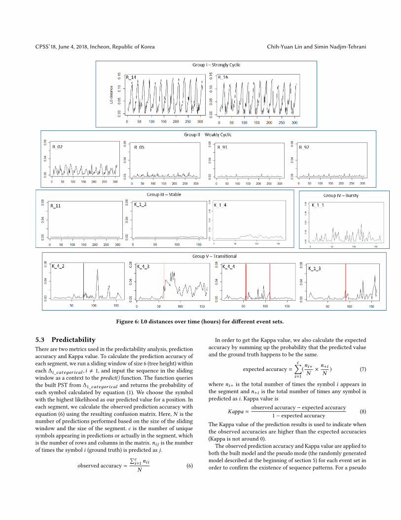
Figure 6 shows the changes of L0 distance over time for differentevent sets from Table 1. We observed five groups of traffic pattern.The group I event sets contain strongly cyclic patterns of changein the distribution of inter-arrival times. The group II event setscontain weakly cyclic patterns in the sense that the changes of
the distribution are relatively small. The group III event sets havealmost no change of distribution. The group IV presents irregularbursts over time. Finally, the group V event sets contain a seriesof bursts for a period of time, which are collectively consideredas a phase. The red lines indicate the starting or stopping point ofanother phase.
In order to discover phase transitions, for the group V eventsets, we find the starting and stopping point of another phase bydetecting bursts when the changes of L0 distance exceeds a phasetransition threshold (PTT). We do this by locating the first and lastburst, and setting the interval between the first and last burst asanother phase if the last burst is not found in the end of the eventset.
In order to standardize the threshold selection procedure, weconsider an acceptable deviation ϵ which is small enough so thateven if it accumulates for every symbol it will not signify a phasetransition. This value has to be chosen experimentally and used todetermine phase transition threshold through equation (5).
PTT =m ∗ ϵ2 (5)
wherem is the previously mentioned number of unique symbolslearned in the first segment (Section 4.2).
Next section presents the predictability of event sets in differentgroups, together with the selected ϵ and length of phases for groupV. For the sake of clarity, we refer to the first phase of an event setas ϕ for the following analysis.
CPSS’18, June 4, 2018, Incheon, Republic of Korea Chih-Yuan Lin and Simin Nadjm-Tehrani
Figure 6: L0 distances over time (hours) for different event sets.
5.3 PredictabilityThere are two metrics used in the predictability analysis, predictionaccuracy and Kappa value. To calculate the prediction accuracy ofeach segment, we run a sliding window of size 6 (tree height) withineach ∆i_cateдor ical , i , 1, and input the sequence in the slidingwindow as a context to the predict() function. The function queriesthe built PST from ∆1_cateдor ical and returns the probability ofeach symbol calculated by equation (1). We choose the symbolwith the highest likelihood as our predicted value for a position. Ineach segment, we calculate the observed prediction accuracy withequation (6) using the resulting confusion matrix. Here, N is thenumber of predictions performed based on the size of the slidingwindow and the size of the segment. c is the number of uniquesymbols appearing in predictions or actually in the segment, whichis the number of rows and columns in the matrix. ni j is the numberof times the symbol i (ground truth) is predicted as j.
observed accuracy =∑ci=1 nii
N(6)
In order to get the Kappa value, we also calculate the expectedaccuracy by summing up the probability that the predicted valueand the ground truth happens to be the same.
expected accuracy =c∑i=1(ni+N× n+i
N) (7)
where ni+ is the total number of times the symbol i appears inthe segment and n+i is the total number of times any symbol ispredicted as i . Kappa value is
Kappa =observed accuracy − expected accuracy
1 − expected accuracy(8)
The Kappa value of the prediction results is used to indicate whenthe observed accuracies are higher than the expected accuracies(Kappa is not around 0).
The observed prediction accuracy and Kappa value are applied toboth the built model and the pseudo mode (the randomly generatedmodel described at the beginning of section 5) for each event set inorder to confirm the existence of sequence patterns. For a pseudo
Understanding IEC-60870-5-104 Traffic Patternsin SCADA Networks CPSS’18, June 4, 2018, Incheon, Republic of Korea
model we expect the Kappa values to be around 0 and for a builtmodel we expect the Kappa values and prediction accuracies to behigher than the values produced by the pseudo model due to thepresence of repeated sequences.
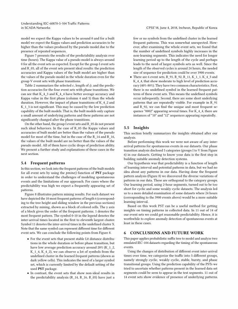
Figure 7 presents the results of the predictability analysis overtime (hours). The Kappa value of a pseudo model is always around0 for all the event sets as expected. Except for the group I event setsand R_05, all of the event sets present ideal results: the predictionaccuracies and Kappa values of the built model are higher thanthe values of the pseudo model in the whole duration even for thegroup V event sets with phase transitions.
Table 2 summarizes the selected ϵ , length of ϕ, and the predic-tion accuracies for the four event sets with phase transitions. Wecan see that K_4_3 and K_4_4 have better average accuracy andKappa value in the first phase (column 4 and 5) than the wholeduration. However, the impact of phase transitions of K_4_2 andK_1_3 is not significant. This may be caused by the low predictioncapability of the built models. That is, the built models only capturea small amount of underlying patterns and these patterns are notsignificantly changed after the phase transitions.
On the other hand, the group I event sets and R_05 do not presentsuch ideal behaviors. In the case of R_05 the Kappa values andaccuracies of built model are better than the values of the pseudomodel for most of the time, but in the case of the R_14 and R_16,the values of the built model are no better than the values of thepseudo model. All of them have cyclic drops of prediction ability.We present a further study and explanations of these cases in thenext section.
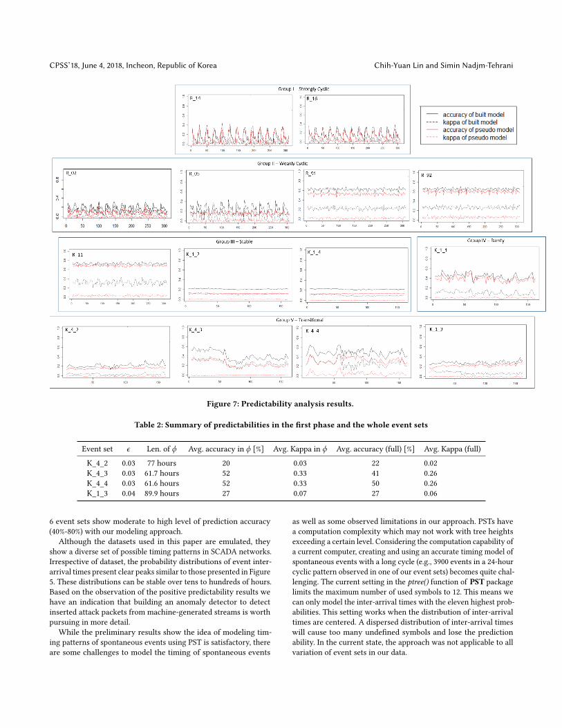
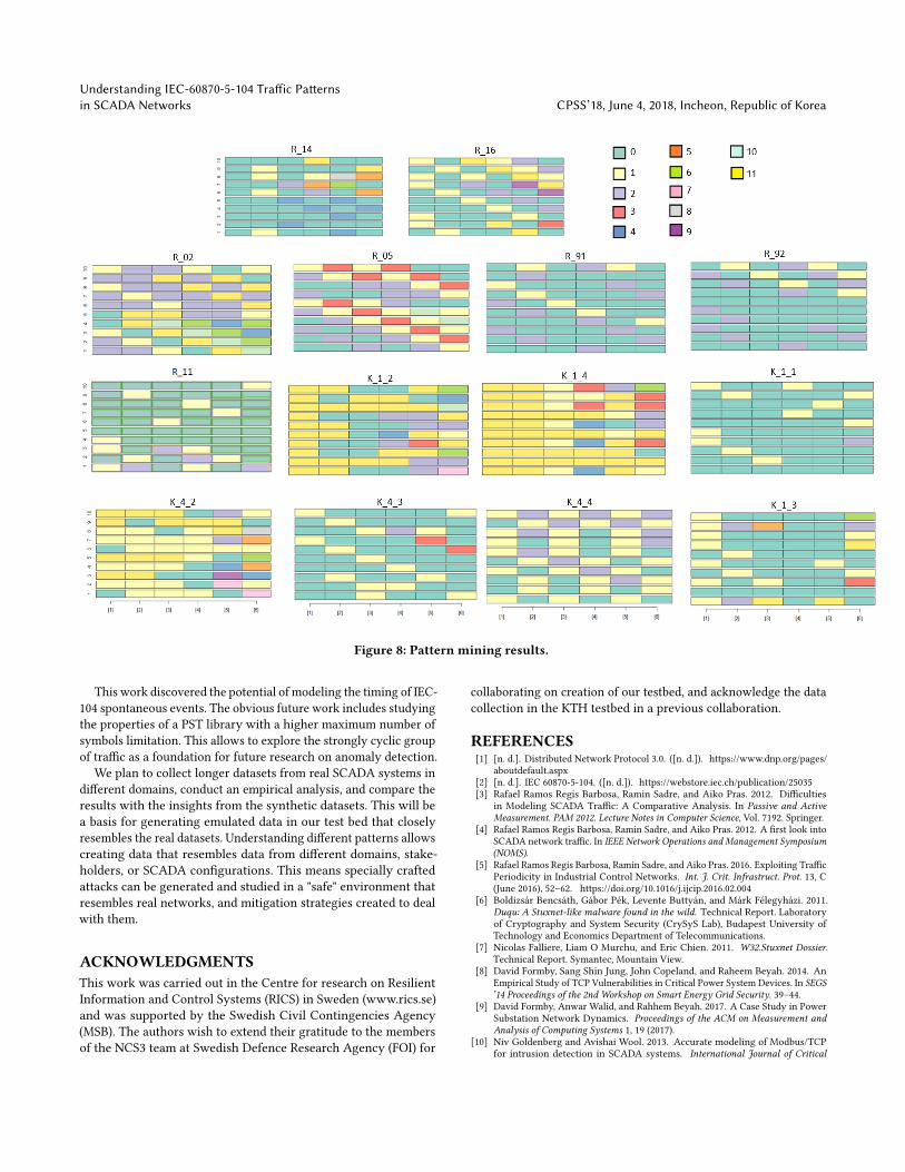
5.4 Frequent patternsIn this section, we look into the frequent patterns of the built modelsfor all event sets by using the pmine() function of PST packagein order to understand the challenges of modeling spontaneousevents and the limitations of our approach. For cases where thepredictability was high we expect a frequently appearing set ofpatterns.
Figure 8 illustrates pattern mining results. For each dataset wehave depicted the 10 most frequent patterns of length 6 (correspond-ing to the tree height and sliding window in the previous sections)extracted by mining, shown as a block of colored cells. The y axisof a block gives the order of the frequent patterns. 1 denotes themost frequent pattern. The symbol 0-10 in the legend denotes theinter-arrival times located in the first to eleventh largest cluster.Symbol 11 denotes the inter-arrival times in the undefined cluster X.Note that the same symbol can represent different time for differentevent sets. We can conclude the following points from Figure 8.
• For the event sets that present stable L0 distance distribu-tions in the whole duration or before phase transition, buthave low average prediction accuracy around 20% (K_1_2,K_1_4, K_4_2), we can observe a lot of symbols from theundefined cluster in the learned frequent patterns (shown asdark yellow cells). This indicates the need of a larger symbolset, which is currently limited by the default setting of theused PST package.• In contrast, the event sets that show non-ideal results inthe predictability analysis (R_14, R_16, R_05) have just a
few or no symbols from the undefined cluster in the learnedfrequent patterns. This was somewhat unexpected. How-ever, after examining the whole event sets, we found thatthe number of undefined symbols highly increases in thenon-learning segments. This indicates the need for longerlearning period up to the length of the cycle and perhapsleads to the need of larger symbols sets as well. Since thelength of the observed cycles is around 24 hours, the neededsize of sequence for prediction could be over 3900 events.• There are 6 event sets, R_91, R_92, R_11, K_1_1, K_4_3 andK_4_4, that show moderate to high level of prediction accu-racy (40%-80%). They have two common characteristics. First,there is no undefined symbol in the learned frequent pat-terns of these event sets. This means the undefined symbolsoccur infrequently. Second, there are some short underlyingpatterns that are repeatedly visible. For example in R_91and R_92, we can find the unique and most frequent se-quence "0002" appearing several times. For K_4_4, there areinstances of "10" and "12" sequences appearing repeatedly.
5.5 InsightsThis section briefly summarizes the insights obtained after ouranalysis.
Before performing this work we were not aware of any inter-arrival patterns for spontaneous events in our datasets. Our phasetransition analysis disclosed 5 categories (groups I to V from Figure6) in our datasets. Getting to know your data is the first step inbuilding suitable anomaly detection systems.
Our hypothesis was that predictability is a function of lengthof learning interval and potential patterns in data, but we had noidea about any patterns in our data. Having done the frequentpattern analysis (Figure 8) we discovered the diverse variations ofpatterns in our data. These are orthogonal to the category groups.Our learning period, using 2-hour segments, turned out to be tooshort for cyclic and some weakly cyclic datasets. The analysis ledus to a more detailed examination of some datasets where 24 hours(corresponding to the 3900 events above) would be a more suitablelearning interval.
Based on this work PST can be a useful method for gettinginsights on timing patterns in collected data. In 11 out of 14 ofour event sets we could get reasonable predictability. Hence, it isworthwhile to explore anomaly detection of spontaneous events atleast in these cases.
6 CONCLUSIONS AND FUTUREWORKThis paper applies probabilistic suffix tree to model and analyze twoemulated IEC-104 datasets regarding the timing of the spontaneousevents.
Using the changes of distribution of different event inter-arrivaltimes over time, we categorize the traffic into 5 different groups,namely strongly cyclic, weakly cyclic, stable, bursty, and phasetransitional groups. Using the prediction capability of the PSTs wetried to ascertain whether patterns present in the learned data setsegments could be seen to appear in the test segments. 11 out of14 event sets show evidence of presence of underlying patterns.
CPSS’18, June 4, 2018, Incheon, Republic of Korea Chih-Yuan Lin and Simin Nadjm-Tehrani
Figure 7: Predictability analysis results.
Table 2: Summary of predictabilities in the first phase and the whole event sets
Event set ϵ Len. of ϕ Avg. accuracy in ϕ [%] Avg. Kappa in ϕ Avg. accuracy (full) [%] Avg. Kappa (full)
6 event sets show moderate to high level of prediction accuracy(40%-80%) with our modeling approach.
Although the datasets used in this paper are emulated, theyshow a diverse set of possible timing patterns in SCADA networks.Irrespective of dataset, the probability distributions of event inter-arrival times present clear peaks similar to those presented in Figure5. These distributions can be stable over tens to hundreds of hours.Based on the observation of the positive predictability results wehave an indication that building an anomaly detector to detectinserted attack packets from machine-generated streams is worthpursuing in more detail.
While the preliminary results show the idea of modeling tim-ing patterns of spontaneous events using PST is satisfactory, thereare some challenges to model the timing of spontaneous events
as well as some observed limitations in our approach. PSTs havea computation complexity which may not work with tree heightsexceeding a certain level. Considering the computation capability ofa current computer, creating and using an accurate timing model ofspontaneous events with a long cycle (e.g., 3900 events in a 24-hourcyclic pattern observed in one of our event sets) becomes quite chal-lenging. The current setting in the ptree() function of PST packagelimits the maximum number of used symbols to 12. This means wecan only model the inter-arrival times with the eleven highest prob-abilities. This setting works when the distribution of inter-arrivaltimes are centered. A dispersed distribution of inter-arrival timeswill cause too many undefined symbols and lose the predictionability. In the current state, the approach was not applicable to allvariation of event sets in our data.
Understanding IEC-60870-5-104 Traffic Patternsin SCADA Networks CPSS’18, June 4, 2018, Incheon, Republic of Korea
Figure 8: Pattern mining results.
This work discovered the potential of modeling the timing of IEC-104 spontaneous events. The obvious future work includes studyingthe properties of a PST library with a higher maximum number ofsymbols limitation. This allows to explore the strongly cyclic groupof traffic as a foundation for future research on anomaly detection.
We plan to collect longer datasets from real SCADA systems indifferent domains, conduct an empirical analysis, and compare theresults with the insights from the synthetic datasets. This will bea basis for generating emulated data in our test bed that closelyresembles the real datasets. Understanding different patterns allowscreating data that resembles data from different domains, stake-holders, or SCADA configurations. This means specially craftedattacks can be generated and studied in a "safe" environment thatresembles real networks, and mitigation strategies created to dealwith them.
ACKNOWLEDGMENTSThis work was carried out in the Centre for research on ResilientInformation and Control Systems (RICS) in Sweden (www.rics.se)and was supported by the Swedish Civil Contingencies Agency(MSB). The authors wish to extend their gratitude to the membersof the NCS3 team at Swedish Defence Research Agency (FOI) for
collaborating on creation of our testbed, and acknowledge the datacollection in the KTH testbed in a previous collaboration.
aboutdefault.aspx[2] [n. d.]. IEC 60870-5-104. ([n. d.]). https://webstore.iec.ch/publication/25035[3] Rafael Ramos Regis Barbosa, Ramin Sadre, and Aiko Pras. 2012. Difficulties
in Modeling SCADA Traffic: A Comparative Analysis. In Passive and ActiveMeasurement. PAM 2012. Lecture Notes in Computer Science, Vol. 7192. Springer.
[4] Rafael Ramos Regis Barbosa, Ramin Sadre, and Aiko Pras. 2012. A first look intoSCADA network traffic. In IEEE Network Operations and Management Symposium(NOMS).
[5] Rafael Ramos Regis Barbosa, Ramin Sadre, and Aiko Pras. 2016. Exploiting TrafficPeriodicity in Industrial Control Networks. Int. J. Crit. Infrastruct. Prot. 13, C(June 2016), 52–62. https://doi.org/10.1016/j.ijcip.2016.02.004
[6] Boldizsár Bencsáth, Gábor Pék, Levente Buttyán, and Márk Félegyházi. 2011.Duqu: A Stuxnet-like malware found in the wild. Technical Report. Laboratoryof Cryptography and System Security (CrySyS Lab), Budapest University ofTechnology and Economics Department of Telecommunications.
[7] Nicolas Falliere, Liam O Murchu, and Eric Chien. 2011. W32.Stuxnet Dossier.Technical Report. Symantec, Mountain View.
[8] David Formby, Sang Shin Jung, John Copeland, and Raheem Beyah. 2014. AnEmpirical Study of TCP Vulnerabilities in Critical Power System Devices. In SEGS’14 Proceedings of the 2nd Workshop on Smart Energy Grid Security. 39–44.
[9] David Formby, Anwar Walid, and Rahhem Beyah. 2017. A Case Study in PowerSubstation Network Dynamics. Proceedings of the ACM on Measurement andAnalysis of Computing Systems 1, 19 (2017).
[10] Niv Goldenberg and Avishai Wool. 2013. Accurate modeling of Modbus/TCPfor intrusion detection in SCADA systems. International Journal of Critical
[11] Sang Shin Jung, David Formby, Carson Day, and Raheem Beyah. 2015. A first lookat machine-to-machine power grid network traffic. In Smart Grid Communications(SmartGridComm), 2014 IEEE International Conference on.
[12] Amit Kleinmann and Avishai Wool. 2014. Accurate Modeling of the Siemens S7SCADA Protocol for Intrusion Detection and Digital Forensic. The Journal ofDigital Forensics, Security and Law 9, 2 (2014).
[13] Amit Kleinmann and Avishai Wool. 2016. A Statechart-Based Anomaly Detec-tion Model for Multi-Threaded SCADA Systems.. In International Conference onCritical Information Infrastructures Security (CRITIS 2015).
[14] Abdun Naser Mahmood, Christopher Leckie, Jiankun Hu, Zahir Tari, and Mo-hammed Atiquzzaman. 2010. Network Traffic Analysis and SCADA Security.Handbook of Information and Communication Security (2010), 383–405.
[15] sKyWIper Analysis Team. 2012. sKyWIper (a.k.a. Flame a.k.a. Flamer): A complexmalware for targeted attacks. Technical Report. Laboratory of Cryptography andSystem Security (CrySyS Lab), Budapest University of Technology and EconomicsDepartment of Telecommunications.
[16] Robert Udd, Mikael Asplund, Simin Nadjm-Tehrani, Mehrdad Kazemtabrizi, andMathias Ekstedt. 2016. Exploiting Bro for IntrusionDetection in a SCADASystem..In CPSS ’16 Proceedings of the 2nd ACM International Workshop on Cyber-PhysicalSystem Security.
[17] Alfonso Valdes and Steven Cheung. 2009. Communication pattern anomalydetection in process control systems. In IEEE Conference on Technologies forHomeland Security. (HST ’09).