Understanding the genetic architecture of complex traits ...

Understanding the genetic architecture of complex traitsthrough SNP-based heritability analysis

David Balding1,3 and Doug Speed2,3

1 Melbourne Integrative Genomics, Schools of BioSciences and of Maths & Stats, University of Melbourne2 Aarhus Institute of Advanced Studies, Aarhus University

3 University College London Genetics Institute.

MIG Workshop, University of Melbourne11 Dec 2018

1 GWAS: review of main concepts

2 What is heritability?

3 Heritability based on SNPs: the GCTA model

4 SNP-heritability and MAF

5 SNP-heritability and LD: the LDAK model

6 Comparison of GCTA and LDAK models

7 Genotype certainty and rare variants

8 Heritability of genome parts: enrichment

9 Heritability analyses using summary statistics: LDSC

10 Generalising the heritability model: SumHer

11 Confounding bias in Large-Scale GWAS

12 Comparison of LDSC and Sumher: enrichment of functional categories

13 Genomic prediction: MultiBLUP

Genome wide association study (GWAS)

Over the past ≈12 years, major transformative development in biomedical science.

robust identification of association: genomic loci ⇔ outcomes e.g. disease statusgenomes don’t usually vary over the lifespan, so direction of causality is clearopportunities for confounding are limited + good strategies for addressing them.

GWAS “Manhattan plot” (Ikram MK et al PLoS Genetics 2010).

Overview of GWAS

In a Genome-Wide Association Study (GWAS) n individuals are recorded for:

genotypes at m markers (usually Single-Nucleotide Polymorphisms, SNPs), and

trait(s) that may be categorical (e.g. case/control) or quantitative (numerical values).

Ascertainment: Individuals may be chosen based on trait value(s), which can affect theanalysis.

e.g. in case/control studies, cases are usually oversampled because in a populationrandom sample they would be too rare for a well-powered analysis.

Imputation: In addition to (typically 0.5M to 1M) directly genotyped SNPs there are nowpowerful methods to impute the genotypes at typically 5M to 10M SNPs.

including many SNPs with low MAF (= minor allele fraction);

uncertainty in imputed genotypes can be important, so they should be modelled asrandom variables; however most often low-quality SNPs are weeded out and theremaining SNP genotypes are regarded as known with certainty.

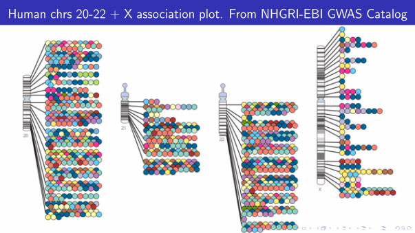
Human chrs 20-22 + X association plot. From NHGRI-EBI GWAS Catalog

Is the GWAS glass half-full or half-empty? The omnigenic world

Despite the success at placing coloured dots on chromosomes,

most GWAS SNPs have very low effect sizes

fine-mapping the exact causal variant is very difficult

in most cases the functional mechanism remains unclear.

In addition to the classical genetics terms monogenic, oligogenic and polygenic, recently1

the term omnigenic has been coined to describe a genetic architecture in which

causal variants are dispersed almost everywhere in the genome

most have a small effect on observed outcome that is mediated through complexpathways offering little opportunity for intervention.

It has been estimated that there is a causal variant for height in every Mb of the humangenome (> 3 000 Mb).

1Boyle, Li & Pritchard, Cell 2017.

The GWAS community’s response to the omnigenic world

Ever bigger sample sizes: 5K was big 10 years ago, 50K was big 5 years ago, today wehave the 500K UK Biobank.

More genetic markers, enhanced by imputation from sequenced genomes: 500K SNPsused to be a lot, now 10M is routine:

almost all SNPs with population minor allele fraction (MAF) above about 0·005.

Meta-analysis: combining results over studies of similar phenotypes in similar populations.

Instead of just one outcome, analyse intermediate phenotypes and/or multiple, relatedoutcomes.

Instead of just one SNP at a time, analyse all genome-wide SNPs simultaneously.

Further problems:

Computation time can be a bottleneck with 500K individuals × 10M SNPs × multipleoutcomes × multiple studies.

Data sharing hindered by data privacy issues: typically only summary statistics at eachSNP are available, not individual-level data.

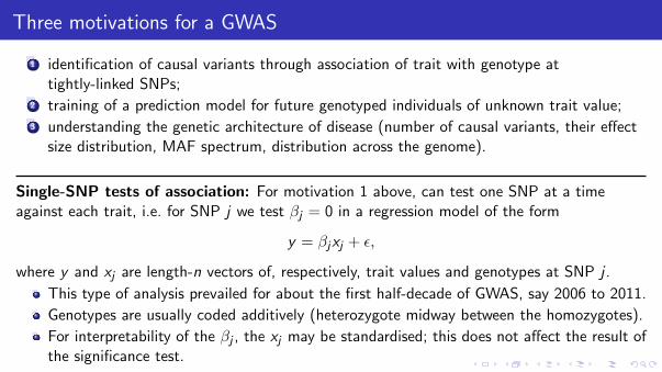
Three motivations for a GWAS

1 identification of causal variants through association of trait with genotype attightly-linked SNPs;

2 training of a prediction model for future genotyped individuals of unknown trait value;3 understanding the genetic architecture of disease (number of causal variants, their effect

size distribution, MAF spectrum, distribution across the genome).

Single-SNP tests of association: For motivation 1 above, can test one SNP at a timeagainst each trait, i.e. for SNP j we test βj = 0 in a regression model of the form

y = βjxj + ε,

where y and xj are length-n vectors of, respectively, trait values and genotypes at SNP j .

This type of analysis prevailed for about the first half-decade of GWAS, say 2006 to 2011.

Genotypes are usually coded additively (heterozygote midway between the homozygotes).

For interpretability of the βj , the xj may be standardised; this does not affect the result ofthe significance test.

Genome-wide statistical models: overfitting

Nowadays single-SNP tests are being superseded by genome-wide statistical models e.g.

y =m∑j=1

βjxj + ε. (1)

Usually m� n and so the βj cannot be estimated without further assumptions. Possiblesolutions:

1 Select m′ ≤ n SNPs, e.g. by thresholding on p-values from single-SNP association.

2 Bayesian regression: prior distribution on the βj with most probability close to zero.

3 Empirical Bayes: similar to 2 above but the “prior” distribution depends on parameter(s)(e.g. effect size variance, Var[βj ]) estimated from the data.

4 Shrinkage/penalised regression: similar to 3 above but rather than derive a posteriordistribution for the βj , just maximise the posterior density to obtain point estimates β̂j .The prior distribution on the βj is often called a penalty function and the posterior densityis called the penalised likelihood.

Sparse and omnigenic models

Early attempts at genome-wide models were driven by a belief in sparsity: almost all the βj arezero.

e.g. the Lasso implements a double exponential prior on the βj with a sharp peak at zero;the posterior is also maximised at zero unless the signal of association is large.

The “omnigenic” model of complex traits involves weak contributions from very many SNPs.

Independent Gaussian (normal) prior distributions on the βj provide acomputationally-feasible omnigenic model.

Any such models incorporate arbitrary aspects (e.g. why should the βj be exponential orGaussian?) but we can check model fit and propose improvements:

Model parameters can be estimated e.g. using maximum likelihood; then compare fittedmodels via likelihood.

Models adequacy can be investigated by comparing properties of simulated and real data.

The predictive performance of a model can be checked, for example using cross validation.

Heritability (h2): definition

Informally, heritability is an attempt to quantify the old “nature versus nurture” issue:

How much variation in an observed trait is attributable to genetics rather thanenvironment?

Narrow-sense heritability h2 is the fraction of phenotypic variance explained in a regressionmodel by (additive) genetic variants:

y =∑j

βjzj + ε (2)

where zj is a vector of genotypes at the jth variant (coded additively), and βj is its effect size.

(2) is similar to (1) but sums over all genome variants whether genotyped/imputed or not.

Problems:

we don’t observe all the causal variants, and we can’t identify which SNPs are causal.

even if we did, we still can’t estimate the βj well, too many predictors ⇒ over-fitting.

Heritability: pedigree-based inference in mixed models

Historic (clever) solution (avoids need for genotype data): random effect regression (ormixed model) with correlation structure defined by pedigree-relatedness

y = γ + ε where γ ∼ N(0, σ2gK ) and ε ∼ N(0, σ2e I ) (3)

where K is an n× n “kinship” matrix computed from identity-by-descent (IBD) probabilities ina pedigree, and I is the identity matrix. Then h2 = σ2g/(σ2g+σ2e ).

Rationale: K ≈ expected genome-wide allele sharing across individuals, which reflects theexcess allele sharing (beyond random draws) that generates phenotypic correlation.Inference of σ2g , σ2e and h2:

REML: maximum likelihood adjusted to reduce bias due to nuisance parameters, orHaseman-Elston (HE) regression:

(yi−yi ′)2 = a + bKii ′ + εii ′ (4)

for all pairs of individuals i and i ′. Then h2 = −b/a.HE is less statistically efficient than REML if the REML assumptions hold, but it is morerobust and computationally easy, whereas REML is infeasible for very large datasets.

Problems with computing K from pedigrees

The mixed model/pedigree approach worked well over decades in animal/plant breeding, butthere are problematic assumptions, including:

Correlation in trait value depends on actual allele sharing, but pedigrees (at best) onlygive expected allele sharing, and the variance of actual allele sharing can be large.

The expected allele sharing is only for a specific pedigree:

the answer depends on choice of pedigree;there is no such thing as a complete or ideal pedigree.

For many years these limitations were overlooked because there was no good alternative.

Pedigrees are still often regarded as defining ”true” relatedness, but in fact there is nodefinitive measure of relatedness;

Nowadays we can measure actual allele sharing from genome-wide SNPs (or sequences).

But there are many ways to compute a SNP-based “kinship”.

See: Speed & Balding (2015) “Relatedness in the post-genomic era: is it still useful?” NatRev Genet 16(1), 33-44. doi:10.1038/nrg3821

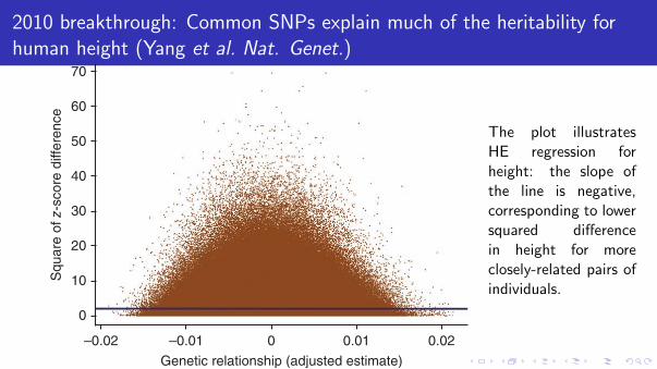
2010 breakthrough: Common SNPs explain much of the heritability forhuman height (Yang et al. Nat. Genet.)

568 VOLUME 42 | NUMBER 7 | JULY 2010 NATURE GENETICS

A N A LY S I S

especially if they have low MAF, will not be in perfect LD with the assayed SNPs. This reduces the power of a conventional GWAS to detect them and reduces the variance estimated for the SNPs col-lectively in our study. The results imply that most causal variants explain such a small proportion of the variance that many causal variants affecting height must exist. The results of published GWASs are consistent with this finding, as high test statistics are distributed over much of the genome16.

Could our results be biased because of ascertainment in the data, data analysis or interpretation? We carefully adjusted phenotypes for systematic differences and applied thorough quality control to the SNP data (Online Methods). We show by principal component analysis (PCA) of African, Asian and European populations that all of our samples are of European ancestry (Supplementary Fig. 2a,b). We demonstrate further by PCA of European populations only that our samples show close relationship to the UK population and do not show an apparent cline across Europe (Supplementary Fig. 2c,d). We performed REML analysis by fitting the first two, four and ten eigenvectors from the European-only PCA as covariates. The results show little to no systematic difference in the estimates of the variance explained by fitting up to ten eigenvectors (Supplementary Table 1). Furthermore, we performed single-SNP association analysis between 1,286 ancestry-informative markers (AIMs) and height, and did not detect a significant inflation of the test statistic for these AIMs (Supplementary Fig. 3; P = 0.219). All these results suggest that our estimate of variance explained by all SNPs is unlikely to be biased by population stratification. A subtle form of stratification in GWASs might occur if subjects are distantly related. We excluded any subject with a relationship to another subject >0.025. If distant pedigree rela-tionships were an important cause of the estimated relationships, then all chromosomes of a pair of subjects should reflect this relationship. We found no correlation between relatedness estimated from different chromosomes (Supplementary Table 2). Thus, the relationships we estimate from SNPs are driven by LD among the SNPs. It is the same LD that causes a SNP that is not a causal variant to show an associa-tion with a trait such as height. In other words, our estimate of the variance explained by the SNPs is based on the same phenomenon as the SNP associations reported from GWASs (LD between SNPs and causal variants). However, we accumulate the variance explained by all SNPs and so are not limited by the need for individual SNPs to pass stringent significance tests.

We also verified that the estimates of variance explained by the SNPs are not driven by a few outlier individuals who are similar in height and in SNP genotypes (Fig. 3). We regressed the squared dif-ference in height between each pair of individuals on the estimate of their relatedness. The intercept and slope are estimates of twice the phenotypic variance and minus twice the additive genetic vari-ance explained by the SNPs, respectively23, so the estimate of variance explained by the SNPs from this regression analysis is ~0.51. The signal on the slope of the regression line comes from many points

and is not due to a few outliers. Note that our maximum likelihood estimate is more accurate than this regression analysis; we show the latter only to illustrate the robustness of the estimate. In addition, we performed REML analysis using subsets of individuals by randomly splitting the whole sample into two and four groups and by sampling 1,000, 2,000 and 3,000 individuals with replacement for four replicates (Supplementary Fig. 4). The average estimates of variance explained by all SNPs are not affected by sample size, but, as expected, the sam-pling error increases as sample size decreases.

Heritability is the proportion of phenotypic variation due to addi-tive genetic factors24; we therefore fitted a model in which SNPs have additive effects. Non-additive genetic variation and variation due to gene-environment interactions may exist, but they are not part of the missing heritability because they do not contribute to the heritability. Epigenetic mutations may cause resemblance between relatives and contribute to heritability if stably inherited, but in that case they would be equivalent to DNA sequence variants, would show LD with the assayed SNPs and would not contribute to missing heritability25.

The method we have presented could be misinterpreted as a method for estimating the heritability of height. Actually, we estimate the variance in height explained by the SNPs. We show that these SNPs do explain over half the estimated heritability of height and that the missing proportion can be explained by incomplete LD between the SNPs and causal variants.

If other complex traits in humans, including common diseases, have genetic architecture similar to that of height, then our results imply that larger GWASs will be needed to find individual SNPs that are significantly associated with these traits, because the variance typically explained by each SNP is so small. Even then, some of the genetic variance of a trait will be undetected because the genotyped SNPs are not in perfect LD with the causal variants. Deep resequenc-ing studies are likely to uncover more polymorphisms, including causal variants that will be represented on future genotyping arrays. Our data provide strong evidence that the variation contributed by many of these causal variants is likely to be small and that very large sample sizes will be required to show that their individual effects are statistically significant. A similar conclusion was drawn recently for schizophrenia26. In some cases the small variance will be due to a large effect for a rare allele, but this will still require a large sample size to reach significance. Genome-wide approaches like those used in our study can advance understanding of the nature of complex-trait variation and can be exploited for selection programs in agriculture27 and individual risk prediction in humans28.

METHODSMethods and any associated references are available in the online version of the paper at http://www.nature.com/naturegenetics/.

–0.01 0 0.01 0.02Genetic relationship (adjusted estimate)

–0.02

70

60

50

Squ

are

of z

-sco

re d

iffer

ence

40

30

20

10

0

Figure 3 All pairwise comparisons contribute to the estimate of genetic variance. Shown are the squared z-score differences between individuals ( y jk

2 ) plotted against the adjusted estimates of genetic relationship (Ajk* ).

The blue line is the linear regression line of y jk2 on Ajk

* . The intercept and regression coefficient are estimates of twice the phenotypic variance and minus twice the genetic variances23, respectively. The intercept is 1.98 (s.e. = 0.001), and the regression coefficient is −1.01 (s.e. = 0.27), consistent with estimates of the phenotypic and additive genetic variance of 0.990 and 0.505, respectively, and a proportion of variance explained by all SNPs of 0.51.

© 2

010

Nat

ure

Am

eric

a, In

c. A

ll ri

ghts

res

erve

d.

The plot illustratesHE regression forheight: the slope ofthe line is negative,corresponding to lowersquared differencein height for moreclosely-related pairs ofindividuals.

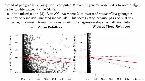
Instead of pedigree-IBD, Yang et al. computed K from m genome-wide SNPs to obtain h2SNP,the heritability tagged by the SNPs.

In the mixed model (3), K = XXT/m where X = matrix of standardised genotypes.They only include unrelated individuals. This seems crazy, because pairs of relativesconvey the most information for estimating the regression slope, as indicated below:

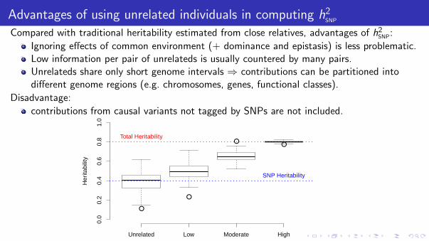
Advantages of using unrelated individuals in computing h2SNP

Compared with traditional heritability estimated from close relatives, advantages of h2SNP:

Ignoring effects of common environment (+ dominance and epistasis) is less problematic.Low information per pair of unrelateds is usually countered by many pairs.Unrelateds share only short genome intervals ⇒ contributions can be partitioned intodifferent genome regions (e.g. chromosomes, genes, functional classes).

Disadvantage:

contributions from causal variants not tagged by SNPs are not included.

●

●

●●

Levels of Relatedness

Her

itabi

lity

0.0

0.2

0.4

0.6

0.8

1.0

Unrelated Low Moderate High

SNP Heritability

Total Heritability

GCTA: Yang et al. Am J Hum Genet 2011

The software GCTA implementing the Yang et al. approach has been very popular.

GCTA underlies many Nature Genetics papers for a few years from 2011.

Results from the method seemed to help “rescue” GWAS from criticism and partly solvethe “missing heritability” problem:

genome-wide significant SNPs explain very little phenotypic variance for a complex trait, buttypically h2SNP > h2/2.

Each entry in the SNP-based kinship matrix K = XXT/m can be interpreted as agenome-wide average of n = 1 allele correlation estimates. K is sometimes called a “genomicrelatedness matrix” (GRM).

It has come to be regarded by many as the definitive SNP-based measure of kinship, butthere is no strong basis for this claim.

The term GRM is misleading in suggesting that it is the “correct” SNP kinship value.

We prefer “genomic similarity matrix” (GSM): the name indicates that there are manypossible choices for K .

Justification for GRM: kinships based on hypothetical, short pedigrees

C

Gene PoolAllele fractionsp and 1!pA

C

A

A

C

A A C A A A A A A

Many population geneticsmodels define kinship interms of allelic correlationbecause it can be shown toequal pedigree kinship

if individuals come from afinite pedigree withunrelated founders, andif allele probabilities infounders are known.

Some population genetics authors put much weight on this theory, but

the underpinning assumptions don’t hold in natural populations;

negative allelic correlations arise in practice yet pedigree kinship is positive by definition.

Problems with SNP kinships

1 In many populations, everyone is closely related:

any two haploid human genomes share over 99.9% sequence identity due to shared ancestry;

but SNPs are chosen to be highly polymorphic. Therefore:

measures of similarity can depend sensitively on the MAF spectrum;more low-MAF sites ⇒ more similarity;MAF spectrum depends on SNP chip and QC.

2 There are many SNP-based measures of the genetic similarity of two individuals.

Which one best captures the phenotypic covariances Var[γ] ?The answer will vary with the genomic architecture of the trait.One option is to optimise e.g. the likelihood within a class of possible K (e.g. optimising overgenotype scaling parameter α discussed below) but over-fitting can be a problem.

A brief survey of possible SNP-kinships

1 Average haplotype sharing. Useful in some settings, but small (e.g. < 1Mb) sharedfragments are informative (because there are many of them) but hard to utilise.

2 Genome-wide averages of single-SNP similarities.Using matches of observed alleles (sometimes called identity by state, IBS) in analogy withIBD probabilities in pedigrees, we average the following scores:

(0, 0) or (2, 2) → 1(0, 1), (1, 1) and (1, 2) → 0·5

(0, 2) → 0

where the SNP genotypes of the two individuals are coded as 0,1 and 2, with 1 =heterozygote.Disagreement about how to code heterozygotes: PLINK codes (1,1) as 1, rather than 0·5.

3 A 1-parameter family of “kinship coefficients” for individuals i and i ′ with genotypes Xij

and Xi ′j at SNP j with MAF pj :

1

m

m∑j=1

(Xij − 2pj)(Xi ′j − 2pj)× [pj(1−pj)]α

α = 0 centred, unscaled genotypes; popular in plant and animal breeding.α = −1 gives allelic correlations used by Yang et al.; upweights low-MAF SNPs; popular forSNP-based h2 estimation in human genetics.Different values of α correspond to different assumptions about the genome-wideMAF–effect size relationship.α can be optimised (e.g. by maximising likelihood) to best reflect the distribution of effectsizes for the trait of interest.

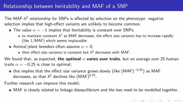
Relationship between heritability and MAF of a SNP

The MAF-h2 relationship for SNPs is affected by selection on the phenotype: negativeselection implies that high-effect variants are unlikely to become common.

The value α = −1 implies that heritability is constant over SNPs;

to maintain constant h2 as MAF decreases, the effect size variance has to increase rapidly(like 1/MAF) which seems implausible.

Animal/plant breeders often assume α = 0;

then effect size variance is constant but h2 decreases with MAF.

We found that, as expected, the optimal α varies over traits, but on average over 25 humantraits α = −0.25 is close to optimal;

this implies that the effect size variance grows slowly (like (MAF)−0.25) as MAFdecreases, so that h2 declines like (MAF)0.75.

Further research can improve this model;

MAF is closely related to linkage disequilibrium and the two need to be modelled together.

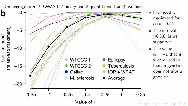
On average over 19 GWAS (17 binary and 2 quantitative traits), we find:

© 2

017

Nat

ure

Am

eric

a, In

c., p

art o

f Spr

inge

r N

atur

e. A

ll ri

ghts

res

erve

d.

4 ADVANCE ONLINE PUBLICATION NATURE GENETICS

A RT I C L E S

than GCTA), whether we used A = −1 (instead of A = −0.25) or whether we analyzed the UCLEB traits, it remained the case that the LDAK model better predicted the heritability contribution of each tranche than the GCTA model.

Relationship between heritability and genotype certaintyThe LDAK model assumes that SNP heritability contributions vary with genotype certainty (measured by the information score, rj). Thus far, our analyses have used only very high-quality SNPs (rj ≥ 0.99), so this assumption has been redundant. We now also include lower-quality, common SNPs; we focus on the UCLEB traits, as for these we were earlier able to test for correlation between genotyping errors and phenotype (Supplementary Fig. 13). Supplementary Table 5 com-pares model fit with and without allowance for genotype certainty; it shows that including rj in the heritability model tends to provide a modest improvement in model fit, resulting in a higher likelihood for 18 of the 31 traits.

Estimates of hSNP2 for the GWAS traits

Table 1 presents our final estimates of hSNP2 for the 19 GWAS traits,

obtained using the LDAK model (with A = −0.25). For comparison, we include previously reported estimates of hSNP

2 , as well as the proportion

of phenotypic variance explained by SNPs reported as genome-wide significant (Supplementary Table 6). For the disease traits, estimates are on the liability scale, obtained by scaling according to the observed case/control ratio and (assumed) trait prevalence26,27. We were unable to find previous estimates of hSNP

2 for tuberculosis or intraocular pres-sure, indicating that, for these two traits, we are the first to establish that common SNPs contribute sizable heritability. Extended results are provided in Supplementary Table 7. These show that our final estimates of hSNP

2 were on average 43% (s.d. 3%) and 25% (s.d. 2%) higher, respectively, than those obtained using the original versions (with A = −1) of GCTA28 and GCTA-LDMS15. Results for the UCLEB traits are provided in Supplementary Table 1.

Role of DNase I hypersensitivity sitesGusev et al.7 used SNP partitioning to assess the contributions of SNP classes defined by functional annotations. Across 11 diseases, they concluded that the majority of hSNP

2 was explained by DNase I hypersensitivity sites (DHSs), despite these containing fewer than 20% of all SNPs. For Figure 5, we performed a similar analysis using the ten traits we had in common with their study (for nine of these, we used the same data). When we copied Gusev et al. and assumed the GCTA model with A = −1, we estimated that on average DHSs

MAF0.01 0.10 0.20 0.30 0.40 0.50

Genotype scaling� = −1� = −0.25� = 0

Per-SNP h2

predicted by �

Log

likel

ihoo

d(r

elat

ive

to m

axim

um)

−1.25 −1 −0.75 −0.5 −0.25 0 0.25

−20

−15

−10

−5

0

WTCCC 1WTCCC 2CeliacM. sclerosis

EpilepsyTuberculosisIOP + WRATAverage

Est

imat

e of

per-

SN

P h

2 (r

elat

ive)

Value of �

a

b

Figure 2 Relationship between heritability and MAF. (a) The parameter A specifies the assumed relationship between heritability and MAF: in human genetics, A = −1 is typically used (solid blue line), while in animal and plant genetics A = 0 is more common (orange); we instead found that A = −0.25 (red) provides a better fit to real data. The gray bars report (relative) estimates of the per-SNP heritability for SNPs with MAF < 0.1 and MAF ≥ 0.1, averaged across the 19 GWAS traits (vertical lines provide 95% confidence intervals); the dashed lines indicate the per-SNP heritability predicted by each A value. (b) For each tranche, we compare A on the basis of likelihood; higher likelihood indicates better-fitting A. Lines report log likelihoods from LDAK for seven values of A, relative to the highest observed likelihood. Line colors indicate the seven trait categories, while the black line reports averages. M. sclerosis, multiple sclerosis; IOP, intraocular pressure; WRAT, wide-range achievement test.

LDSC GCTA GCTA-MS LDAK

0.0

0.5

1.0

1.5

2.0

2.5

GCTA-LDMS

0.0

0.2

0.4

0.6

0.8

1.0

GCTA phenotypes LDAK phenotypes

GCTA

LDAKGCTA-MS

LDAK-MSGCTA-LDMS

Est

imat

e of

h2 S

NP (

rela

tive

to G

CT

A)

WTCCC 1

WTCCC 2

Celiac

M. sclerosis

Epilepsy

Tuberculosis

IOP + WRAT

Average

Est

imat

e of

h2 S

NP

Simulated h2SNP

a

b

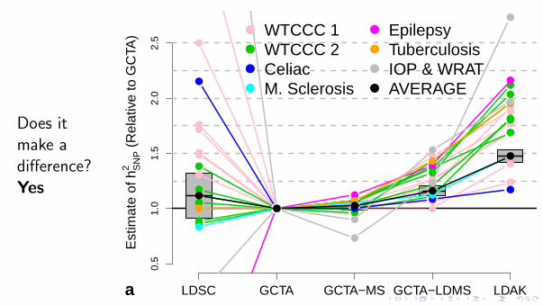
Figure 3 Comparison of methods for estimating hSNP2 for real and

simulated data. (a) Relative estimates of hSNP2 for the GWAS traits. hSNP

2 estimates from LDSC, GCTA-MS (SNPs partitioned by MAF), GCTA-LDMS (SNPs partitioned by LD and MAF) and LDAK are reported relative to those from GCTA. For versions of GCTA and LDAK, we use A = −0.25 (see main text for explanation of A). Line colors indicate the seven trait categories; the black line reports the (inverse-variance-weighted) averages, with gray boxes providing 95% confidence intervals for these averages. Numerical values are provided in Supplementary Table 3. (b) Phenotypes were simulated with 1,000 causal SNPs and hSNP

2 = 0.8 (black horizontal line) and then analyzed using GCTA, GCTA-MS, GCTA-LDMS, LDAK and LDAK-MS (LDAK with SNPs partitioned by MAF). Bars report average hSNP

2 across 200 simulated phenotypes (vertical lines provide 95% confidence intervals). Left, copying the study of Yang et al.15, causal SNP effect sizes are sampled from N(0,1), similar to the GCTA model. Right, causal SNP effect sizes are sampled from N(0,wj), similar to the LDAK model.

likelihood ismaximised forα ≈ −0.25.

The interval[-0.5,0] is wellsupported.

The valueα = −1 that iswidely used inhuman geneticsdoes not give agood fit.

Minor Allele Frequency

Est

imat

e of

Per

−S

NP

h2 (

Rel

ativ

e)

0.01 0.10 0.20 0.30 0.40 0.50

Genotype scaling

α = −1α = −0.25α = 0

a

Per−SNP h2

predicted by α

Illustration of the impli-cations of different MAFscalings α for SNPs par-titioned into MAF < 0.1and MAF > 0.1.

Curves: the (theoretical)per-SNP h2 as a functionof MAF for 3 values of α.

Dashed lines: average val-ues over each part.

Grey: average values overmany GWAS datasets(95% interval in black).

The GCTA genome-wide regression model

The mixed model (3), which underlies GCTA, can be derived from the genome-wide regression(1) in the special case βj ∼ N(0, σ2g/m), independently for each SNP j . Call this (1)*.

Switching between (3) and (1)* can be very useful.

Only (3) was available for pedigree-based h2, and it retains computational advantages.

(1)* is more interpretable: every SNP has an effect (which may be small) either due tobeing directly causal or through tagging causal variants.

Model (1)* is similar to the definition of heritability (2), but now

only genotyped/imputed SNPs included, not all genome variants;

there is an independent and identically-distributed (iid) Gaussian prior βj ∼ N(0, σ2g/m).

The iid assumption was inherited from (3), but is implausible:

multiple SNPs can tag the same causal variant, so their effects are correlated;

we have already established that the βj vary with MAF, perhaps also other factors?

Binary traits: liability model

The analyses discussed so far don’t work well for ascertained case-control studies.We can use (3) or (1)* treating the case/control status as a 0/1 numeric value, theresulting heritability estimate can depend on both the population proportion of cases πand the sample proportion of cases p.

A trick to overcome this problem is to imagine an underlying continuous variable L such thatan individual i is a case if and only Li > T , where T is a threshold determined by the traitprevalence.

Heritability on the observed (O) and liability (L) scales; HE regression

It turns out that h2O , heritability based on the 0/1 observations, is related to liabilityheritability h2L via

h2L = h2O ×π2(1−π)2

p(1−p)z2,

where z is the standard normal density at T .

So we can proceed by computing h2O and then transforming to h2L.

Instead of REML, Golan et al. PNAS (2014) recommended HE regression (4), adapted forbinary traits using the above transformation.

called PCGC: Phenotype Correlation Genotype Correlation.

The name implies the use of allelic-correlation kinships.

The intuition is that allelic correlations are natural to predict phenotypic correlations.But any SNP-based measure of genome-wide similarity can be used.

Problems for SNP-heritability analysis

h2SNP estimates can be inflated by

population structure/cryptic relatedness

Possible remedy: compare h2SNP from all SNPs with sum of values over a partition.

genotyping errors, which can be particularly important when cases and controls aregenotyped separately.

Some testing is possible (e.g. for quantitative traits in multiple cohorts).The problem can be ameliorated using very strict quality control on genotypes, for example ahigh threshold on imputation scores.But strict QC results in loss of information.

Published criticisms of GCTA

Browning & Browning, Am J Hum Genet (2011): h2SNP sensitive to population structure. Didnot note the partition test.

Kumar et al. PNAS (2016) “Limitations of GCTA as a solution to the missing heritabilityproblem”. They make several criticisms:

some can be attributed to insufficiently strict QC;

others reflect basic misunderstandings, see e.g. blog by Gusev;

they noted that GCTA does not include correlations in the βj due to LD.

Speed et al. Am J Hum Genet (2012): reported that h2SNP estimates are robust to

number of causals, causal MAF spectrum, effect size distribution,

but ...

h2SNP

estimates not robust to linkage disequilibrium (LD)

●

●

●

●

●

●

Tagging of Causal SNPs

Her

itabi

lity

Estim

ates

from

50

Rep

licat

es

0.0

0.2

0.4

0.6

0.8

1.0

Very Weak Weak Average Strong Very Strong Very Weak Weak Average Strong Very Strong

Standard Kinship Matrix Weighted Kinship Matrix

Local level of LD

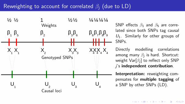
LD is statistical dependencebetween pairs of SNPs.

If an extra SNP is genotypedin high LD with an existingSNP tagging a causal, thenpart of the contribution toh2SNP from that causal isdouble-counted:“over-tagging”.

This can occur whether ornot the causal variant is itselfgenotyped.

Reweighting to account for correlated βj (due to LD)

Adjusting for Uneven Tagging

Genotyped SNPs

Underlying Variation

β1β

5β

2β

3β

6β

8β

7β

8

U1

U2

U3

U4

X1

X2

X3

X4

X1

X3

X4X

4

Weightings½ ½ 1 ½½ ¼¼¼

β9

¼

X4

We suggest calculating weighted allelic correlations.

Nobel Prize Speech 20th May 2015 [email protected]

Weights

Genotyped SNPs

Causal loci

SNP effects β1 and β5 are corre-lated since both SNPs tag causalU1. Similarly for other groups ofSNPs.

Directly modelling correlationsamong many βj is hard. Shortcut:weight Var[βj ] to reflect only SNPj ’s independent contribution.

Interpretation: reweighting com-pensates for multiple tagging ofa SNP by other SNPs (LD).

SNPs X1 X2 X3 X4 X5 X6 X7 X8 X9 X10

GCTA Model 5 5

High CorrelationLow Correlation

LDAK Model 4.6 1.9

Region 21

Expected (relative) contribution to hSNP

of each region:2

Weights 1.0 0.8 0.8 1.0 1.0 1.0 0 0.9 0 0

Reweighting improves estimation of h2SNP

●

●

●

●

●

●

Tagging of Causal SNPs

Her

itabi

lity

Est

imat

es fr

om 5

0 R

eplic

ates

0.0

0.2

0.4

0.6

0.8

1.0

Very Weak Weak Average Strong Very Strong Very Weak Weak Average Strong Very Strong

Standard Kinship Matrix Weighted Kinship Matrix

Implemented in LDAK, world’s most popular software for computing LD-Adjusted Kinships,h2SNP estimation and prediction http://ldak.org

Yang et al. (2015) Nat Genet 47, 1114-20

©20

15N

atur

e A

mer

ica,

Inc.

All

righ

ts r

eser

ved.


A N A LY S I S

for LD heterogeneity, for example, the LDAK approach16, which gives each variant a weight according to the LD r2 value between the vari-ant and all other variants in the region, and the LD residual (LDres) approach15,17, which uses the residuals from a linear regression of each variant on a set of LD-pruned variants in the region. However, the LDAK adjustment resulted in a substantial overestimation of hWGS

2 , regardless of whether the variants were stratified by MAF (Fig. 1). This is because the LDAK adjustment created a strong negative corre-lation between the weights and MAFs of the variants (Supplementary Fig. 2), such that rare variants, which tend to have lower LD with sur-rounding variants, received too much weight. We also observed small biases using LDres and MAF-stratified LDres (LDres-MS) (Fig. 1). We propose a method (Online Methods), termed LD- and MAF-stratified GREML (GREML-LDMS), which uses a sliding window approach to fit the region-specific LD heterogeneity across the genome (Fig. 2). We demonstrate by analyzing simulated data, under four different scenarios, that the GREML-LDMS estimates of hWGS

2 are unbiased, regardless of the MAF and LD properties of causal variants (Fig. 1) and the number of LD and MAF groups (Supplementary Fig. 3). The heritability parameter used in all the simulations above was 0.8. We show that all the conclusions hold irrespective of the size of the heritability parameter used for simulation (Supplementary Table 1).

Variation at whole-genome sequence variants captured by 1000 Genomes Project imputationWe have quantified above the (un)biased nature of GREML methods in estimating hWGS

2 under different simulation scenarios. In practice, however, there have not been whole-genome sequencing data available with a sample size that is sufficiently large to estimate hWGS

2 with useful precision. However, there are a large number of GWAS samples avail-able that have been imputed to the 1000 Genomes Project reference panels. We therefore addressed the question of how much variation at sequence variants could be captured by imputing GWAS genotype data to the 1000 Genomes Project reference panels. From UK10K-WGS data, we extracted the genotypes of variants represented on the Illumina CoreExome array and then imputed the genotype data to the 1000 Genomes Project reference panels (Online Methods). We used the GREML-MS approach (seven genetic components) to esti-mate the variance explained by the 1000 Genomes Project–imputed variants (h1KGP2 ) for the simulated phenotype (1,000 causal variants randomly sampled from all sequence variants) (Online Methods). We know from the simulation results presented above that, under this scenario (that is, where causal variants are sampled completely at random), all three GREML methods—GREML-SC, GREML-MS and GREML-LDMS—are unbiased. We chose to use GREML-MS because it is able to provide estimates of variance explained for variants in different MAF groups with standard errors smaller than those from GREML-LDMS (Supplementary Table 1). The results showed that the proportion of variation at variants from whole-genome sequenc-ing captured by 1000 Genomes Project imputation decreased with more stringent thresholds for imputation accuracy (the INFO metric

imputing the SNP array data to the 1000 Genomes Project reference panels10, where h hWGS 1KGP

2 2 because of the loss of tagging due to imperfect imputation. We previously developed the single- component GREML analysis (GREML-SC) method (based on a single genetic relationship matrix, or GRM) as implemented in GCTA11 to estimate the proportion of variance explained by all common SNPs in a GWAS sample of unrelated individuals12. To quantify the amount of variation at sequence variants that could be captured by 1000 Genomes Project imputation, we first needed to investigate whether this approach could provide an unbiased estimate of herit-ability using whole-genome sequencing data. We performed exten-sive simulations based on a whole-genome sequencing data set from the UK10K project13 (UK10K-WGS), which comprised 17.6 million genetic variants (excluding singletons and doubletons) in 3,642 unre-lated individuals after quality controls (Online Methods). The simu-lation results showed that, if causal variants were a random subset of all the sequence variants (52.7% rare), the GREML-SC estimate of hWGS

2 using all variants (including the causal variants) was unbiased (Fig. 1), consistent with our theoretical derivation (Supplementary Note). By ‘unbiased’, we mean that the mean estimate of hWGS

2 from 200 simulation replicates was not significantly different from the h2 parameter used for simulation. We could also expect from the theoretical derivation that, if causal variants had a different MAF spectrum than the variants used in the analysis, the GREML-SC estimate of hWGS

2 would be biased. This was demonstrated using simulations (Online Methods): if we randomly sampled disproportionally rare (or common) variants as causal variants, the estimate of hWGS

2 was biased downward (or upward) (Fig. 1). This problem has been discussed previously12 and can be solved by MAF-stratified GREML (GREML-MS) analysis14 (Online Methods). We show by simulations that the estimate of hWGS

2 from GREML-MS was unbiased, irrespective of the MAF spectrum of the causal variants (Fig. 1).

We know from the theoretical derivation (Supplementary Note) that GREML-SC is biased if causal variants have a different LD prop-erty than the variants used in the analysis. A difference in LD can be caused by a difference in the MAF spectrum, which can be cor-rected for using the GREML-MS approach, as shown above. However, GREML-MS is unable to correct for the region-specific LD hetero-geneity across the genome (Supplementary Fig. 1). That is, if causal variants tend to be enriched in genomic regions with higher or lower LD than average, the estimate of h2 from either GREML-SC or GREML-MS will be biased. We confirmed this using simulations where, if all causal variants were sampled from the variants at DNase I–hypersensitive sites (DHSs) (Online Methods), which have systemati-cally lower LD than average15, the GREML-MS estimate of hWGS

2 was biased downward (Fig. 1). Methods have been developed to adjust

1.2

1.0

0.8

Her

itabi

lity

estim

ate

0.6

0.4

0.2

0Random More common Rarer Rarer + DHS

GREML-SCGREML-MSLDAKLDAK-MSLDresLDres-MSGREML-LDMS

Figure 1 Estimates of heritability using sequence variants under different simulation scenarios based on the UK10K-WGS data set. Each column represents the mean estimate from 200 simulations. Error bars, s.e.m. The true heritability parameter was 0.8 for the simulated trait. Four simulation scenarios are shown: random causal variants are sampled at random; more common causal variants are more frequent than random variants; rarer causal variants are less frequent than random variants; rarer + DHS causal variants are all in DHSs and are less frequent than random variants (see the Online Methods for more details on the simulation scenarios).

Simulation study findsthat LDAK performspoorly and GCTA per-forms well.

This seemed alarming,so we investigated ...

Est

imat

e of

hS

NP

2

0.0

0.2

0.4

0.6

0.8

1.0

GCTA Phenotypes LDAK Phenotypes

Simulated hSNP2

GCTA LDAK

GCTA−MS LDAK−MS

GCTA−LDMS

B

We found that Yang et al. only sim-ulated under the GCTA model (left).

The assumption of norelationship between h2 andLD has been made by manyprevious authors, but our workshowed that estimates can besensitive to this assumption.

We did the same in reverse andshowed that GCTA performs badlyunder the LDAK model (right).

So the models are very different,which one better reflects reality? Weneed to check against real data. Alot of data . . .

Model fit to real data: difference in ln(likelihood) LDAK-GCTA

Wellcome Trust CCC Traits n (K) diff eMerge Traits n (K) diff

Bipolar Disorder 4.8 29.0 Age-related Macular Disease 8.5 3.2Coronary Artery Disease 4.9 6.2 Heart Failure 9.0 5.2

Crohn’s Disease 4.7 20.4 Peripheral Arterial Disease 10.5 5.5Hypertension 4.9 14.7 Shingles (Herpes Zoster) 14.0 −1.3

Rheumatoid Arthritis 4.8 6.2 Venous Thromboembolism 12.0 3.7Type I Diabetes 4.9 9.8 Triglyceride 12.1 6.1

Type II Diabetes 4.9 11.4 LDL Cholesterol 13.4 5.3Barrett’s Oesophagus 7.0 14.4 HDL Cholesterol 13.8 24.6

Celiac Disease 9.9 22.1 Systolic Blood Pressure 15.1 3.1Ischaemic Stroke 9.0 41.0 Diastolic Blood Pressure 15.1 2.9

Parkinson’s Disease 6.9 −4.8 Height 18.2 50.9Psoriasis 7.5 37.3 Body Mass Index 19.3 51.8

Ulcerative Colitis 8.0 40.7

Average 9.7 16.4

25 GWAS with low confounding, mean 3.6M SNPs (range 2.1M – 4.6M), MAF > 0.01.

© 2

017

Nat

ure

Am

eric

a, In

c., p

art o

f Spr

inge

r N

atur

e. A

ll ri

ghts

res

erve

d.

NATURE GENETICS ADVANCE ONLINE PUBLICATION 5

A RT I C L E S

contributed 86% (s.d. 4%) of hSNP2 , close to the value they reported

(79%). When instead we assumed the LDAK model (with A = −0.25), the estimated contribution of DHSs was reduced to 25% (s.d. 2%). Under the LDAK model, DHSs were predicted to contribute 18% of hSNP

2 , so 25% represents a 1.4-fold enrichment. To add context, we also considered ‘genic’ SNPs, which we define as SNPs inside or within 2 kb of an exon (using RefSeq annotations29), and ‘intergenic’ SNPs further than 125 kb from an exon; these definitions ensure that these two SNP classes are also predicted to contribute 18% of hSNP

2 under the LDAK model. We estimated that genic SNPs contributed 29% (s.d. 2%), while intergenic SNPs contributed 10% (s.d. 2%), representing 1.6-fold and 0.6-fold enrichment, respectively. When we extended this analysis to all 42 traits, DHSs on average contributed 24% (s.d. 2%) of hSNP

2 , and, in contrast to Gusev et al., enrichment remained constant when we reduced SNP density (Supplementary Figs. 14 and 15, and Supplementary Table 8).

Finucane et al.30 performed a similar analysis but considered 52 SNP classes and estimated enrichment using LDSC; across nine traits, they identified five classes with >4-fold enrichment, the highest of which, ‘conserved SNPs’, had 13-fold enrichment. When we used LDAK to estimate enrichment for our 19 GWAS traits, the results were more modest; the highest enrichment was 2.5-fold, with only 1.3-fold enrichment for conserved SNPs (Supplementary Fig. 16).

Relaxing quality controlFor the UCLEB data, we considered nine alternative SNP filtering set-tings. Supplementary Figure 17 reports estimates of hSNP

2 for each trait–filtering combination, while Figure 6a provides a summary. First, we varied the information score (rj) threshold to greater than 0.99, 0.95, 0.9, 0.6, 0.3 and 0 (each time continuing to require MAF ≥ 0.01). Simulations suggested that, by including all 8.8 million com-mon SNPs (rj ≥ 0) instead of using just the 353,000 high-quality ones (rj ≥ 0.99), we can expect estimates of hSNP

2 to increase by 50–60% (Supplementary Fig. 18). This is similar to what we observed in prac-tice, as across the 23 traits estimates of hSNP

2 (using A = −0.25) were on average 45% (s.d. 8%) higher. The simulations further predicted that, even though the Metabochip provides relatively low coverage of the genome (after quality control, it contains only ~60,000 SNPs, predom-inantly within genes), we can expect estimates of hSNP

2 to be approxi-mately 80% as high as those obtained starting from genome-wide genotyping arrays. While we were unable to test this claim directly, it is consistent with our results for height, BMI and QT Interval, the

three traits for which reasonably precise estimates of common SNP hSNP

2 are available6 (Fig. 6b). For the final three SNP filtering set-tings, we varied the MAF threshold to be greater than 0.0025, 0.001 and 0.0005 (all with rj ≥ 0). Across the 23 traits, we found that rare SNPs contributed substantially to hSNP

2 : for example, when we used the 17.3 million SNPs with MAF ≥ 0.0005, estimates of hSNP

2 (using A = −0.25 and MAF partitioning) were on average 29% (s.d. 12%) higher than those based on the 8.8 million common SNPs (median increase 22%), with rare SNPs contributing on average 33% (s.d. 5%) of hSNP

2 (Fig. 6a).

DISCUSSIONWith estimates of hSNP

2 so widely reported, it is easy to forget that calculating the variance explained by large numbers of SNPs is a chal-lenging problem. To avoid overfitting, it is necessary to make strong prior assumptions about SNP effect sizes, but different assump-tions can lead to substantially different estimates of hSNP

2 . Previous attempts to assess the validity of assumptions have used simulation studies14,15, but this approach will tend to favor assumptions similar to those used to generate the phenotypes. Instead, we have compared different heritability models empirically, by examining how well they fit real data sets.

We began by investigating the relationship between heritability and MAF. Across 42 traits, we found that the best fit was achieved by setting A = −0.25 in model (1), which implies that average herit-ability varies with (MAF(1 – MAF))0.75. As explained in the Online Methods, the value of A corresponds to the scaling of genotypes. Therefore, our result indicates that the performance (detection power and/or prediction accuracy) of many penalized and Bayesian regres-sion methods, for example, Lasso, ridge regression and BayesA31,32, could be improved simply by changing how genotypes are scaled. Although we recommend A = −0.25 as the default value, with suf-ficient data available, it should be possible to estimate A on a trait-by-trait basis or to investigate more complex relationships between heritability and MAF. In particular, with a better understanding of the relationship between heritability and MAF for low frequencies, it may no longer be necessary to partition by MAF when rare SNPs are included.

We also examined the relationship between heritability and LD. Thus far, most estimates of hSNP

2 have been based on the GCTA model;

0

20

40

60

80

100C

ontr

ibut

ion

of lo

w-L

D tr

anch

e (%

)

WTCCC 1WTCCC 2CeliacM. sclerosis

EpilepsyTuberculosisIOP + WRATAverage

Predicted under LDAK modelPredicted under GCTA model

Low-LD tranche contains 50% of SNPs Low-LD tranche contains 25% of SNPs

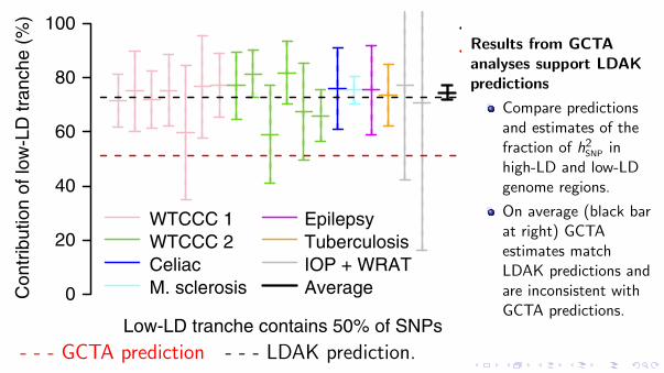
Figure 4 Comparing the GCTA and LDAK models for the GWAS traits. We partition SNPs into those with low or high LD, with the low-LD tranche containing either 50% (left) or 25% (right) of SNPs. For each partition, the horizontal red and black lines indicate the predicted contribution of the low-LD tranche to hSNP

2 under the GCTA and LDAK models, respectively. Vertical lines provide point estimates and 95% confidence intervals for the contribution of the low-LD tranche to hSNP

2 , estimated assuming the GCTA model. Line colors indicate the seven trait categories, while the black lines provide the (inverse-variance-weighted) averages.

0

50

100

150

DHS (GCTA) DHS (LDAK) Genic (LDAK) Intergenic (LDAK)

Bipolar disorderCoronary artery diseaseCrohn's diseaseHypertensionRheumatoid arthritisType 1 diabetes

Type 2 diabetesSchizophreniaUlcerative colitisMultiple sclerosisAverageExpected

Con

trib

utio

n of

SN

P c

lass

to h

2 SN

P (

%)

Figure 5 Enrichment of SNP classes. Block 1 reports the contributions to hSNP

2 of DHSs, estimated under the GCTA model with A = −1 (see the main text for explanation of A). The vertical lines provide point estimates and 95% confidence intervals for each trait and for the (inverse-variance-weighted) average; for three of the traits, the point estimate is above 100%, as was also the case for Gusev et al.7. Block 2 repeats this analysis but now assuming the LDAK model with A = −0.25. Blocks 3 and 4 estimate the contribution of genic SNPs (those inside or within 2 kb of an exon) and intergenic SNPs (further than 125 kb from an exon), again assuming the LDAK model with A = −0.25. To assess enrichment, estimated contributions are compared to those expected under the GCTA or LDAK model, as appropriate (horizontal lines).

Results from GCTAanalyses support LDAKpredictions

Compare predictionsand estimates of thefraction of h2SNP inhigh-LD and low-LDgenome regions.

On average (black barat right) GCTAestimates matchLDAK predictions andare inconsistent withGCTA predictions.

- - - GCTA prediction - - - LDAK prediction.

Does itmake adifference?Yes

LDSC GCTA GCTA−MS LDAK

0.5

1.0

1.5

2.0

2.5

GCTA−LDMS

Est

imat

e of

hS

NP

2 (

Rel

ativ

e to

GC

TA)

●

●●

●

●

●

●●

●

●

●

● ●

●

●

● ●

●

●

●

● ● ●

●

●

● ●●

●

●

●●

●

●

●

●●

●

●

●

●●

●

●

●

● ●

●

●

●●

●

●

●

●

●

●

●

●

●

● ●

●

●

●

● ●

●

●

●

●●

●

●

●

●

●

●

● ●

●

●

●

●

●

●

●

●

●

●

●

●

●

●●

●

●

●

●

●

●

●

●

●

●

WTCCC 1WTCCC 2CeliacM. Sclerosis

EpilepsyTuberculosisIOP & WRATAVERAGE

a

Do we need to stratify on MAF and/or LD?

Subsequent to the original publication of GCTA, modifications were proposed to stratify SNPsfirst on MAF and later on both MAF and LD, so that the iid βj assumption is only madewithin strata. This reduces the problem, but:

the iid assumption is also invalid within strata;

arbitrary strata boundaries,

many additional parameters to estimate,

loss of interpretability – reduced opportunity to understand mechanisms.

We found that GCTA-LDMS achieves about the same total log-likelihood as LDAK overmany studies, at the cost of 19 additional parameters.

The MAF and LD stratifications applied to LDAK lead to small gains in log-likelihood

but improvements can’t justify any additional parameters,

so our MAF and LD adjustments appear adequate by this criterion;

however we do currently recommend partitioning for SNPs with MAF < 1%.

Recap of LD issue and GCTA vs LDAK models

GCTA model assumes a priori that βj ∼ N(0, σ2g/m) for every SNP.

The LDAK model βj ∼ N(0,wjσ2g/W ) fits empirical human data much better, where:

wj is a weight that reflects local levels of LD and W =∑

j wj ;wj tends to be low if the jth SNP is in high LD with nearby SNPs.

In addition to the LD issue, we saw earlier that the allelic-correlation kinship matrix is alsosuboptimal because the α = −1 scaling of genotypes does not adequately model the MAF –effect size relationship for real traits. We found that

α = −0.25 fits well on average over many traits when LDAK weights are included toallow for LD effects.

The optimal α value varies across traits, due to differing selection effects.

For binary traits, we now recommend using LDAK weights in PCGC regression.

This leads to a further ≈ 20% increase in h2SNP estimates.

NB: LDAK model downweights common (well-genotyped) SNPs and upweights rare andpoorly-genotyped SNPs so strict QC is important.

We’ve covered effects of LD and MAF on SNP h2. Anything else?

Genotype certainty is another major factor. We consider:

poorly-genotyped or poorly-imputed common SNPs;

all low-MAF SNPs (MAF < 0.01).

Intuitively, the lower the genotype certainty the lower our prior expected heritability.

Previous analyses have not taken this into account.

It’s common to impose strict QC, but at a high cost in terms of missing true h2.

We propose a measure rj of genotype certainty at the jth SNP. Our heritability model now hasgenotypes scaled with α = −0.25 and

βj ∼ N(0, rjwjσ2g/W ).

Previous analyses have assumed rj = wj = 1 and α = −1.

Need to test for correlation between genotyping errors and phenotype before includinglow-certainty SNPs (rj � 1).

Including rare variants: UCLEB data, 23 quantitative traits, metabochip

© 2

017

Nat

ure

Am

eric

a, In

c., p

art o

f Spr

inge

r N

atur

e. A

ll ri

ghts

res

erve

d.


A RT I C L E S

this model can be motivated by a belief that each SNP is expected to have the same effect on the phenotype, from which it follows that the expected heritability of a region should depend on the number of SNPs it contains. By contrast, the LDAK model views highly correlated SNPs as tagging the same underlying variant and therefore believes that the expected heritability of a region should vary according to the total amount of distinct genetic variation it contains. Across our traits, we found that the relationship between heritability and LD specified by the LDAK model consistently provided a better description of reality.

This finding has important consequences for complex trait genet-ics. First, it implies that, for many traits, common SNPs explain con-siderably more phenotypic variance than previously reported, which represents a major advance in the search for missing heritability2. It also affects a large number of closely related methods. For exam-ple, LDSC10, like GCTA, assumes that heritability contributions are independent of LD, and it therefore also tends to underestimate hSNP

2 . Similarly, we have shown that estimates of the relative importance of SNP classes via SNP partitioning can be misleading when the GCTA model is assumed7,30. Further afield, most software for mixed-model association analyses (for example, FAST-LMM, GEMMA, MLM-LOCO and BOLT) use an extension of the GCTA model33–36, which is also the case for most bivariate analyses, including those performed by

LDSC8,37,38. It remains to be seen how much these methods would be affected if they employed more realistic heritability models.

Attempts have been made to improve the accuracy of heritabil-ity models via SNP partitioning14,15,39. We find that partitioning by MAF can be advantageous, as it guards against misspecification of the relationship between heritability and MAF when rare variants are included. Figure 3a and Supplementary Figure 7 indicate that the realism of the GCTA model can be improved by partitioning based on LD; for example, across the GWAS traits, estimates from GCTA-LDMS are on average 16% (s.d. 2%) higher than those from GCTA and only 23% (s.d. 2%) lower than those from LDAK. The improvement arises because model misspecification is reduced by allowing SNPs in lower-LD tranches to have higher average heritability. However, Supplementary Table 9 illustrates why we consider such an approach suboptimal; in particular, SNP partitioning can be computationally expensive and, even with LD partitioning, model fit tends to be worse than that from LDAK.

While we have investigated the role of MAF, LD and genotype cer-tainty, there remain other factors on which heritability could depend, in particular the available functional annotations of genomes40. For example, our comparison of genic and intergenic SNPs indicates that the effect size prior distribution could be improved by taking into account proximity to coding regions. By way of demonstration, Supplementary Table 10 shows that model fit is improved by assuming E h = c f fj w r D +j k j

+j j j[ ] [ ( )] ( )/2 11 exp( 50 ) r r r r B 500 where Dj

is the distance (in kb) between SNP j and the nearest exon (under this model, genic SNPs are expected to have about twice the heritability of intergenic SNPs). In general, we believe that modifications of this type will have a relatively small impact; we note that, across the 19 GWAS traits, this modification increases model log likelihood by on average only 1.5, much less than the average increase obtained by using A = −0.25 instead of A = −1 (8.9) or by choosing the LD model specified by LDAK instead of GCTA (17.7), and does not significantly change estimates of hSNP

2 . However, with sufficient data, it may be possible to obtain more substantial improvement by tailoring model assumptions to individual traits.

When estimating hSNP2 , care should be taken to avoid possible

sources of confounding. Previously, we advocated a test for infla-tion of hSNP

2 due to population structure and familial relatedness3. The conclusions of a recent paper claiming that hSNP

2 estimates are unreliable41 would have changed substantially had this test been applied (Supplementary Fig. 19). We also recommend testing for inflation due to genotyping errors, particularly before including lower-quality and/or rare SNPs. For the 23 UCLEB traits, we showed that including poorly imputed SNPs resulted in significantly higher estimates of hSNP

2 and made it possible to capture the majority of genome-wide heritability, despite the very sparse genotyping pro-vided by the Metabochip. We found that including rare SNPs also led to significantly higher hSNP

2 . Although sample size prevented us from obtaining precise estimates of hSNP

2 for individual traits, our analyses indicate that, for larger data sets, including rare SNPs will be both practical and fruitful in the search for the remaining miss-ing heritability2.

URLs. LDAK, http://www.ldak.org/; PLINK, http://www.cog-genomics. org/plink2; SHAPEIT, http://www.shapeit.fr/; IMPUTE2, http:// mathgen.stats.ox.ac.uk/impute/impute_v2.html; DHS annotations, http://hgdownload.cse.ucsc.edu/goldenPath/hg19/encodeDCC/wgEncodeRegDnaseClustered/wgEncodeRegDnaseClusteredV3.bed.gz; RefSeq annotations, http://hgdownload.cse.ucsc.edu/goldenPath/hg19/database/refGene.txt.gz.

0.0

0.1

0.2

0.3

0.4

High-qualitycommon SNPs

All commonSNPs

All SNPsno partitioning

All SNPs5 tranches

Scaling parameter �−1.25−0.75−0.25 (advised)0−1−0.50.25Rare variation

0.0

0.2

0.4

0.6

0.8

High-quality common SNPsAll common SNPsAll SNPs

BMI QT intervalHeight

Ave

rage

est

imat

e of

h2 S

NP

Est

imat

e of

h2 S

NP

a

b

Figure 6 Varying quality control for the UCLEB traits. We consider three SNP filtering settings: 353,000 high-quality common SNPs (information score ≥ 0.99, MAF ≥ 0.01), 8.8 million common SNPs (MAF ≥ 0.01) and all 17.3 million SNPs (MAF ≥ 0.0005). (a) Blocks indicate SNP filtering; bars report (inverse-variance-weighted) average estimates of hSNP

2 using LDAK (vertical lines provide 95% confidence intervals). Bar color indicates the value of A used. For blocks 1–3, hSNP

2 is estimated using the non-partitioned model. For block 4, SNPs are partitioned by MAF; we find this is necessary when rare SNPs are included and it also allows estimation of the contribution of SNPs with MAF < 0.01 (hatched areas). (b) Bars report our final estimates of hSNP

2 for height, BMI and QT interval—the three traits for which common SNP heritability has previously been estimated with reasonable precision6 (orange lines mark the 95% confidence intervals from these previous studies). Bar colors now indicate SNP filtering; all estimates are based on A = −0.25, using either a non-partitioned model (red and blue bars) or with SNPs partitioned by MAF (purple bars).

350K SNPs 9M SNPs 17M SNPs

“5 Tranches”refers topartitioning byMAF, which weadvocate forlow-MAF SNPs.

Hatched areasshowcontribution ofSNPs withMAF<0.01.

© 2

017

Nat

ure

Am

eric

a, In

c., p

art o

f Spr

inge

r N

atur

e. A

ll ri

ghts

res

erve

d.


A RT I C L E S

this model can be motivated by a belief that each SNP is expected to have the same effect on the phenotype, from which it follows that the expected heritability of a region should depend on the number of SNPs it contains. By contrast, the LDAK model views highly correlated SNPs as tagging the same underlying variant and therefore believes that the expected heritability of a region should vary according to the total amount of distinct genetic variation it contains. Across our traits, we found that the relationship between heritability and LD specified by the LDAK model consistently provided a better description of reality.

This finding has important consequences for complex trait genet-ics. First, it implies that, for many traits, common SNPs explain con-siderably more phenotypic variance than previously reported, which represents a major advance in the search for missing heritability2. It also affects a large number of closely related methods. For exam-ple, LDSC10, like GCTA, assumes that heritability contributions are independent of LD, and it therefore also tends to underestimate hSNP

2 . Similarly, we have shown that estimates of the relative importance of SNP classes via SNP partitioning can be misleading when the GCTA model is assumed7,30. Further afield, most software for mixed-model association analyses (for example, FAST-LMM, GEMMA, MLM-LOCO and BOLT) use an extension of the GCTA model33–36, which is also the case for most bivariate analyses, including those performed by

LDSC8,37,38. It remains to be seen how much these methods would be affected if they employed more realistic heritability models.

Attempts have been made to improve the accuracy of heritabil-ity models via SNP partitioning14,15,39. We find that partitioning by MAF can be advantageous, as it guards against misspecification of the relationship between heritability and MAF when rare variants are included. Figure 3a and Supplementary Figure 7 indicate that the realism of the GCTA model can be improved by partitioning based on LD; for example, across the GWAS traits, estimates from GCTA-LDMS are on average 16% (s.d. 2%) higher than those from GCTA and only 23% (s.d. 2%) lower than those from LDAK. The improvement arises because model misspecification is reduced by allowing SNPs in lower-LD tranches to have higher average heritability. However, Supplementary Table 9 illustrates why we consider such an approach suboptimal; in particular, SNP partitioning can be computationally expensive and, even with LD partitioning, model fit tends to be worse than that from LDAK.

While we have investigated the role of MAF, LD and genotype cer-tainty, there remain other factors on which heritability could depend, in particular the available functional annotations of genomes40. For example, our comparison of genic and intergenic SNPs indicates that the effect size prior distribution could be improved by taking into account proximity to coding regions. By way of demonstration, Supplementary Table 10 shows that model fit is improved by assuming E h = c f fj w r D +j k j

+j j j[ ] [ ( )] ( )/2 11 exp( 50 ) r r r r B 500 where Dj

is the distance (in kb) between SNP j and the nearest exon (under this model, genic SNPs are expected to have about twice the heritability of intergenic SNPs). In general, we believe that modifications of this type will have a relatively small impact; we note that, across the 19 GWAS traits, this modification increases model log likelihood by on average only 1.5, much less than the average increase obtained by using A = −0.25 instead of A = −1 (8.9) or by choosing the LD model specified by LDAK instead of GCTA (17.7), and does not significantly change estimates of hSNP

2 . However, with sufficient data, it may be possible to obtain more substantial improvement by tailoring model assumptions to individual traits.

When estimating hSNP2 , care should be taken to avoid possible

sources of confounding. Previously, we advocated a test for infla-tion of hSNP

2 due to population structure and familial relatedness3. The conclusions of a recent paper claiming that hSNP

2 estimates are unreliable41 would have changed substantially had this test been applied (Supplementary Fig. 19). We also recommend testing for inflation due to genotyping errors, particularly before including lower-quality and/or rare SNPs. For the 23 UCLEB traits, we showed that including poorly imputed SNPs resulted in significantly higher estimates of hSNP

2 and made it possible to capture the majority of genome-wide heritability, despite the very sparse genotyping pro-vided by the Metabochip. We found that including rare SNPs also led to significantly higher hSNP

2 . Although sample size prevented us from obtaining precise estimates of hSNP

2 for individual traits, our analyses indicate that, for larger data sets, including rare SNPs will be both practical and fruitful in the search for the remaining miss-ing heritability2.

URLs. LDAK, http://www.ldak.org/; PLINK, http://www.cog-genomics. org/plink2; SHAPEIT, http://www.shapeit.fr/; IMPUTE2, http:// mathgen.stats.ox.ac.uk/impute/impute_v2.html; DHS annotations, http://hgdownload.cse.ucsc.edu/goldenPath/hg19/encodeDCC/wgEncodeRegDnaseClustered/wgEncodeRegDnaseClusteredV3.bed.gz; RefSeq annotations, http://hgdownload.cse.ucsc.edu/goldenPath/hg19/database/refGene.txt.gz.

0.0

0.1

0.2

0.3

0.4

High-qualitycommon SNPs

All commonSNPs

All SNPsno partitioning

All SNPs5 tranches

Scaling parameter �−1.25−0.75−0.25 (advised)0−1−0.50.25Rare variation

0.0

0.2

0.4

0.6

0.8

High-quality common SNPsAll common SNPsAll SNPs

BMI QT intervalHeight

Ave

rage

est

imat

e of

h2 S

NP

Est

imat

e of

h2 S

NP

a

b

Figure 6 Varying quality control for the UCLEB traits. We consider three SNP filtering settings: 353,000 high-quality common SNPs (information score ≥ 0.99, MAF ≥ 0.01), 8.8 million common SNPs (MAF ≥ 0.01) and all 17.3 million SNPs (MAF ≥ 0.0005). (a) Blocks indicate SNP filtering; bars report (inverse-variance-weighted) average estimates of hSNP

2 using LDAK (vertical lines provide 95% confidence intervals). Bar color indicates the value of A used. For blocks 1–3, hSNP

2 is estimated using the non-partitioned model. For block 4, SNPs are partitioned by MAF; we find this is necessary when rare SNPs are included and it also allows estimation of the contribution of SNPs with MAF < 0.01 (hatched areas). (b) Bars report our final estimates of hSNP

2 for height, BMI and QT interval—the three traits for which common SNP heritability has previously been estimated with reasonable precision6 (orange lines mark the 95% confidence intervals from these previous studies). Bar colors now indicate SNP filtering; all estimates are based on A = −0.25, using either a non-partitioned model (red and blue bars) or with SNPs partitioned by MAF (purple bars).

Orange lines indicate95% confidence intervalsfor previous estimates ofh2SNP.

For the purple bars only(all SNPs) the SNPs arepartitioned by MAF.

Genome partitioning example: DNaseI hypersensitivity sites (DHS):

Gusev et al. (2014) used SNP partitioning to assess the contributions of SNPs classed byfunctional annotations.

Across 11 diseases they reported that 79% of h2SNP was explained by DHS, which include< 20% of all SNPs;

a striking 4-fold enrichment;DHS account for almost all non-genic h2SNP.

We perform a similar analysis using the 10 traits we have in common with their study (for9 of these, using the same data) and using their definitions of DHS.

Under the GCTA Model, DHS contribute 86% (SD 4) of h2SNP.

Under the LDAK Model, DHS contribute 25% (SD 2) of h2SNP.

LDAK predicts 18% DHS contribution ⇒ 1.4-fold enrichment.We estimate that genic SNPs contribute 29% (SD 2), representing 1.6-fold enrichment,respectively.Over 42 traits, DHS contribute 24% (SD 2) of h2SNP.

Heritability of genome parts0

5010

015

0

Con

trib

utio

n of

SN

P C

lass

to h

SN

P2

(%

)

DHS (GCTA) DHS (LDAK) Genic (LDAK) Inter−Genic (LDAK)

Bipolar DisorderCoronary Artery DiseaseCrohn's DiseaseHypertensionRheumatoid ArthritisType 1 Diabetes

Type 2 DiabetesSchizophreniaUlcerative ColitisMultiple SclerosisAverageExpected

2015 breakthrough: analysis of all GWAS SNPs using summary statistics

Core idea: the heritability tagged by a SNP increases linearly with its LD (correlation) withlocal SNPs. More local LD ⇒ more tagging of causal variation.a b

c d

Figure 1: Test statistics are correlated with both LD and LDAK Scores. (a) Test statistics versus LD scores from the most recentGiant Consortium meta-analysis for height;12 to avoid correlated datapoints, we restrict to a subset of 121 310 SNPs with MAF>0.01in approximate linkage equilibrium (obtained by pruning so that no two SNPs within 1 cM have r2

jl > 0.2). (b) The correlation canbe magnified by first dividing SNPs into 50 bins based on LD Scores, then plotting mean test statistic versus mean LD score for eachbin.3 (c) The same as (b), except we consider LDAK scores instead of LD Scores. (d) The same as (b), except that instead of using thetest statistics for height, we generate new ones based on the LDAK Model. In each plot, the solid red line is the line of best fit fromleast-squares regression; the dashed red lines and solid blue segments indicate, respectively, 95% confidence intervals for the slope andintercept from this regression.

We can see that this follows from Equation (1) if we assume the GCTA Model (as then v2j has expected value lj h2

SNP/m) and that aj is30

constant across the genome.31

Evidence for the LDAK Model32

In our previous work,1 we performed a careful evaluation of the GCTA and LDAK Models. We collected GWAS data for 42 different33

traits, both binary and quantitative, then performed stringent quality control, checking that any confounding due to population structure34

or cryptic relatedness was at most slight.9, 10 We demonstrated that it was valid to compare models using the REML likelihood, then35

used this approach to show that the LDAK Model was both significantly and substantially more realistic than the GCTA Model; it fit36

better for 37 of the 42 traits (P < 10�7) and resulted in an average increase in log likelihood of 9.8 per trait. We also investigated37

attempts to improve the accuracy of the GCTA Model by partitioning (we focused on GCTA-LDMS,11 but the same arguments apply to38

S-LDSC7). While partitioning allowed GCTA to achieve log likelihoods comparable to those from LDAK, this came at the cost of 1939

extra parameters which were arbitrarily defined, added little to model interpretation and reduced the precision of heritability estimates.40

Evidence for the GCTA Model41

In their correspondence, Gazal et al. make no mention of the evidence we provided in support of the LDAK Model. Instead, their42

rationale for preferring the GCTA Model is the observation that for many traits the marginal effect size of a SNP has been shown to have43

a strong linear dependency on its LD score (in our notation, that there is a significant correlation between lj and Sj). We do not dispute44

that these correlations exist; for example, Figures 1a & 1b demonstrate that lj and Sj are correlated for human height, using data from45

2

a b

c d




















2

2015 breakthrough: analysis of all GWAS SNPs using summary statistics

Core idea: the heritability tagged by a SNP increases linearly with its LD (correlation) withlocal SNPs. More local LD ⇒ more tagging of causal variation.a b

c d




















2

a b

c d




















2

LD Score regression (LDSC)

Bulik-Sullivan et al. Nat Genet 2015a; > 770 google scholar citations

Assuming a polygenic model, LDSC fits a simple linear regression on GWAS summarystatistics Sj :

E[Sj ] = A +n

mh2SNP

∑k

r 2jk (5)

Sj is an association test statistic at SNP j with a χ21 null distribution

A− 1 measures confounding bias (e.g. due to relatedness/pop structure),

n = sample size and m = # SNPs,

h2SNP = heritability tagged by all SNPs,∑k r

2jk = LD Score of SNP j ; the sum is over SNPs in a neighbourhood of j .

LD Hub

/22/bioinformatics.btw613.abstract)

Questions and Help Requests

If you have any bug reports or questions please send an email to Jie Zheng (https://www.researchgate.net/profile/Jie_Zheng12) at [email protected] or [email protected]

Other friendly platforms: MR-Base (http://www.mrbase.org/)

Project members (ordered by first name):Alkes Price (Department of Epidemiology, Harvard T.H. Chan School of Public Health, Boston, Massachusetts,USA)A. Mesut Erzurumluoglu (Genetic Epidemiology Group, Department of Health Sciences, University of Leicester,Leicester, UK)Benjamin Elsworth (MRC Integrative Epidemiology Unit, University of Bristol)Benjamin Neale (Analytic and Translational Genetics Unit, Massachusetts General Hospital)Brendan Bulik-Sullivan (Broad Institute of MIT and Harvard)David Evans (MRC Integrative Epidemiology Unit, University of Bristol; Diamantina Institute, University ofQueensland)Gibran Hemani (MRC Integrative Epidemiology Unit, University of Bristol, Oakfield House, Bristol, UK)Hilary Finucane (Department of Epidemiology, Harvard T.H. Chan School of Public Health, Boston, Massachusetts,USA)Jie Zheng (MRC Integrative Epidemiology Unit, University of Bristol, Oakfield House, Bristol, UK)Katherine Tansey (MRC Integrative Epidemiology Unit, University of Bristol, Oakfield House, Bristol, UK)Laurence Howe (MRC Integrative Epidemiology Unit, University of Bristol, Oakfield House, Bristol, UK)Lavinia Paternoster (MRC Integrative Epidemiology Unit, University of Bristol, Oakfield House, Bristol, UK)Nicole M. Warrington (MRC Integrative Epidemiology Unit, University of Bristol, Oakfield House, Bristol, UK)Philip C. Haycock (MRC Integrative Epidemiology Unit, University of Bristol, Oakfield House, Bristol, UK)Tom Gaunt (MRC Integrative Epidemiology Unit, University of Bristol)Verneri Anttila (Broad Institute of MIT and Harvard)© 2016 Broad Institute

2.7 BillionSNP-Phenotype

associations

>500 millionNumber of individuals

41GWAS consortia

832GWAS studies

LD Hub http://ldsc.broadinstitute.org/ldhub/

2 of 2 8/12/18, 21:17

LD Hub is a database of summary-level GWAS results and a web interface that automatesLDSC analyses to estimate h2SNP, partition it into functional categories, and estimate geneticcorrelations.

Zheng, et al. (2017) Bioinformatics. 33(2): 272-79.

Our critique of LDSC

1 The slope does not give an accurate estimator of h2SNP.

2 Consequently, the intercept is not a good measure of confounding (that would be trueeven without the first problem).

Rationale:

(5) implicitly assumes that every SNP is expected to contribute equally to h2SNP,

thus, SNPs are weighted only by their r2 with SNP j .

Important information is ignored ⇒ results from LDSC are often misleading.

So what’s the problem?

The expected heritability of each SNP varies with properties known a priori.

Essentially the same problem we previously criticised (Speed et al. 2017) in GCTA, whichhas similar uses to LDSC but uses individual genotypes.

Most important property of a SNP is its LD with other SNPs. MAF is also important,and genotype quality, genomic region, ....

LDAK summary-statistic software: SumHer

Instead of assuming E[h2j ] constant over SNPs as in GCTA and LDSC, SumHer allows ageneral heritability model embodied in weights qj that can depend on LD, MAF and otherfactors known a priori (in practice we use LDAK weights).

E[Sj ] = C (1 +n

Qh2SNP

∑k

qk r2jk). (6)

where Q =∑m

j=1 qj . LDSC sets qj = 1 for all j , so that Q = m.

We include a multiplicative C for confounding in place of the additive A.

Estimates of A and C are the same, but this choice affects estimate of h2SNP.

C is similar to genomic control, where Sj are divided by the genome inflation factor, GIF.

Notation in following slides: For both LDSC and Sumher, we use suffixes -ZERO for noconfounding term, -CEPT for A adjustment, -GC for C adjustment.

a b

c d




















2

00.

10.

20.

30.

40.

50.

60.

7

Ave

rage

hS

NP

2True hSNP

2


LDS

C−

Zer

o

LDS

C

Sum

Her

−Z

ero

Sum

Her

−G

C

LDS

C−

Zer

o

LDS

C

Sum

Her

−Z

ero

Sum

Her

−G

C

Checking the models:simulated data.

We compare LDSC andSumHer (both with and with-out intercept) under GCTA andLDAK models.

As expected, both perform wellunder their assumed model butnot under the other model.

Con

trib

utio

n of

Low

−LD

SN

Ps

0.0

0.2

0.4

0.6

0.8

1.0

LDSC (a=0) LDSC SumHer

All 26 Traits (n=120k)12 Binary Traits14 Quantatative Traits

Expected GCTAExpected LDAK Checking the models:

predicted share of h2SNP

inlow-LD SNPs

For a large collection of GWASdatasets we divided small genomicregions into high-LD and low-LD,and compared the estimatedcontribution to h2SNP from each setwith expectations under the GCTAand LDAK models.

SumHer estimates are close to LDAKpredictions, but LDSC values areintermediate between the predictionsof the two models.

Hybrid model: data “choose” between GCTA/LDSC and LDAK/SumHer models.On y axes: 0 = 100% GCTA/LDSC 1 = 100% LDAK/SumHer

(a) (b) (c)

Figure 3: Comparing the GCTA and LDAK Models. These analyses use Hybrid-Zero and Hybrid-GC,

versions of SumHer which assign weights 1-p and p to the GCTA and LDAK heritability models,

respectively. (a) Average estimates of p from Hybrid-Zero for GCTA phenotypes (true p = 0), LDAK

phenotypes (true p = 1) and hybrid phenotypes (true p = 0.5). (b) Estimates of p from Hybrid-Zero for the 25

raw GWAS. Colors distinguish between the 13 WTCCC, the 5 binary eMERGE and 7 quantitative eMERGE

traits (black denotes the 25-trait average). A precise estimate of p was not possible for Shingles (Segment

17), due to the trait having very low h2SNP. (c) Estimates of p from Hybrid-GC for the 24 summary GWAS.

Colors distinguish between the 9 binary and 15 quantitative traits (black denotes the 25-trait average). In

all plots, vertical line segments mark 95% confidence intervals.

Comparing heritability models

Previously, we compared different heritability models based on the likelihood from REML analysis; we

showed that across 42 human traits (average sample size 7400), the log likelihood was on average 9.8 nats

higher if we assumed the LDAK Model rather than the GCTA Model.5 Those 42 traits included the 13

WTCCC traits we study here. If we repeat that analysis using the 12 eMERGE traits (average sample size

13,000), we find that log likelihood is on average 16 nats higher under the LDAK Model (Supplementary

Table 5). To compare heritability models based on REML requires access to individual-level data, but with

SumHer it is possible to compare models when only summary statistics are available; Supplementary Table

6 shows that across the 25 raw GWAS, the log likelihood is on average 17 nats higher under the LDAK

Model. An alternative, easier-to-visualize method is to run SumHer using a hybrid heritability model

containing both the GCTA and LDAK Models, and allow the data to decide the relative weighting of each.

Specifically, we use Hybrid-Zero, with the focus on estimating p, the “proportion of LDAK”, in Model (2).

Figure 3a demonstrates proof of principle, using our simulated phenotypes: we see that Hybrid-Zero

correctly estimates p ≈ 0 when applied to the GCTA phenotypes, p ≈ 1 for the LDAK phenotypes, and p ≈

0.5 for “Hybrid Phenotypes” (created by summing

Phenotypes 1 & 101, 2 & 102, etc.). We then apply Hybrid-Zero to our 25 raw GWAS (Figure 3b and

Supplementary Table 6); the average estimate of p is 1.03 (s.d. 0.02), indicating that the data

overwhelmingly support the LDAK Model over the GCTA Model.

Population structure and relatedness

Until recently, it was standard to estimate confounding bias via the genomic inflation factor11 (GIF).

However, the GIF tends to over-estimate bias, because it makes the assumption that all observed inflation of

test statistics is due to confounding.16 LDSC provides a method for estimating confounding bias which

appreciates that substantial inflation can instead be due to causal variation.1 However, our simulations

indicated that LDSC also tends to over-estimate bias, due to the poor fit of the GCTA heritability model.

This is supported by our analysis of the 25 raw GWAS, for which we performed very careful quality control

and verified using REML that confounding due to population structure and relatedness is modest

(Supplementary Fig. 3). As shown in Supplementary Table 2, the average estimate of confounding bias

from LDSC is 1.033 (s.d. 0.001); although lower than the average GIF (1.058), it nonetheless indicates there

is substantial confounding. By contrast, SumHer-GC finds that confounding is slight; its average estimate of

bias is 1.005 (s.d. 0.002).

We now construct GWAS with substantial confounding. First, for each of the 13 WTCCC GWAS, we replace

2000 of the controls (on average 54%) with 2000 individuals from POBI17 (People of the British Isles); this

generates population structure because, although both WTCCC and POBI individuals were recruited from

the UK, the latter predominately came from isolated, rural regions (Supplementary Fig. 5). As shown in

(a) Simulation proof of principle

(b) GCTA vs LDAK for full GWAS data (mean n = 10K)

(c) LDSC vs SumHer for summary stats (mean n = 121K)

Results: 100% support for LDAK (individual genotypes), around 85% support for SumHer(summary stats) because we can’t do strict enough QC with summary stats.

●

●

●

●

●

●

●

●

●●

●

●

●

●

●

●

●

●

●

●

●

●

● ●

0.00 0.05 0.10 0.15 0.20 0.25

0.0

0.1

0.2

0.3

0.4

0.5

LDSC h^2

Sum

Her

h^2

Alzheimer

CAD

CD

Ever smoked

IBD

RA

Schizophrenia

T2D

UC BMD

BMI

Depressive Symptoms

Fasting Glucose

Glycated Hemoglobin

HDL

Height

LDL

Menarche age

Menopause age

Neuroticism

Subjective Well−Being

Triglyceride

WHRYrs Educ

MEAN OF 24 TRAITS

SumHer h2SNP> LDSC h2

SNP

On average 3-fold higher forthese 24 GWAS datasets withmean n = 121K.

A better-fitting model is ableto detect more signal?

Estimation of GWAS confounding biasDoes the Heritability Model Matter?

Estimates of Confounding

LDSC assumes GCTA Model

SumHer-GC assumes LDAK Model

[email protected] 7th December 2018

Estimation of GWAS confounding bias was theoriginal primary aim of LDSC, using theregression intercept A.

SumHer uses instead multiplicative C : cancorrect any over-conservative genomic control.

Null simulations: LDSC and SumHer correctlyinfer no confounding under their respectivemodels; LDSC infers confounding (A > 1)under the LDAK model while SumHer infersC < 1 under the GCTA model.

Confounding bias in large GWAS (14 of 24 traits shown)

Trait n GIF LDSC A SumHer C

Alzheimer’s Disease 54 000 1.09 1.07 1.03Coronary Artery 80 000 1.10 1.06 0.99Crohn’s Disease 21 000 1.14 1.08 0.97Depressive symptoms 161 000 1.12 1.03 0.96Ever Smoked? 74 000 1.11 1.02 0.96

Bone Mineral Density 33 000 1.11 1.07 1.00Body Mass Index 230 000 1.13 0.80 0.55Fasting Glucose 58 000 1.08 1.04 0.99Glycated Hemoglobin 46 000 1.04 1.03 0.99HDL Cholesterol 96 000 1.03 1.04 0.68Height 246 000 2.09 1.69 0.98LDL Cholesterol 91 000 1.03 1.00 0.73Menarche Age 253 000 1.66 1.21 0.89Menopause Age 69 000 1.10 1.06 0.92

mean (24 traits) 121 000 1.21 1.04 0.93

Average 3.1M SNPsper GWAS (MAF >0.01)

GIF = GenomicInflation Factor =ratio of empiricalmedian to null median

Unlike LDSC, SumHerfinds the originalGWAS tended toover-correct forconfounding.

Number of significant loci after correction (14 of 24 traits shown)

Trait n None GIF LDSC A SumHer C

Alzheimer’s Disease 54 000 21 19 19 21Coronary Artery 79 000 10 6 7 10Crohn’s Disease 21 000 64 52 58 64Ever Smoked? 74 000 0 0 0 0

Bone Mineral Density 33 000 19 18 18 19Body Mass Index 230 000 69 52 135 336Depressive symptoms 161 000 0 0 0 1Fasting Glucose 58 000 22 20 20 23Glycated Hemoglobin 46 000 10 10 10 10HDL Cholesterol 96 000 130 122 121 216Height 246 000 720 196 288 754LDL Cholesterol 91 000 101 96 101 155Menarche Age 253 000 289 111 190 354Menopause Age 69 000 49 39 39 55

mean (24 traits) 121 000 86 46 62 118

Many extra hitsusing SumHer:due to betterheritability model,not the differencebetween A and Cadjustments.

●

●

●

C1 C2 C3

0.0

0.2

0.4

0.6

0.8

1.0

Additive confounding adjustment

a

h SN

P2

●

●

●

●

●

C1 C2 C3

0.0

0.2

0.4

0.6

0.8

1.0

Multiplicative confounding adjustment

b

h SN

P2

●

●

C1 C2 C3

0.95

1.00

1.05

1.10

1.15

Estimated confounding parameter

c

1+A

/C

C1, 10 % confounding C2, 5 % confounding C3, 2 % confounding

●

●

●

●

C1 C2 C3

0.0

0.2

0.4

0.6

0.8

1.0

1.2

Additive confounding adjustment

a

h SN

P2

●

●

●

●

●

C1 C2 C3

0.0

0.2

0.4

0.6

0.8

1.0

1.2

Multiplicative confounding adjustment

b

h SN

P2

●

●●

C1 C2 C30.

951.

001.

051.

101.

15

Estimated confounding parameter

c

1+A

/C

C1, 10 % confounding C2, 5 % confounding C3, 2 % confounding

Warning:problems withconfoundingmodel in bothLDSC (top) andSumher(bottom).

Simulation:Hierarchicalstructuredpopulation with 3subsubpopulationswithin each of 3subpopulations.

a

00.

10.

20.

30.

40.

50.

60.

7

Aver

age

h SNP

2

True hSNP2


LDSC

−Zer

o

LDSC

Sum

Her−Z

ero

Sum

Her−G

C

LDSC

−Zer

o

LDSC

Sum

Her−Z

ero

Sum

Her−G

C

b

01

23

4

Av. E

nric

hmen

t of C

onse

rved

Reg

ions

TrueEnrichment


LDSC

−Zer

o

LDSC

Sum

Her−Z

ero

Sum

Her−G

C

LDSC

−Zer

o

LDSC

Sum

Her−Z

ero

Sum

Her−G

C

c

00.

10.

20.

30.

40.

50.

6

Aver

age

Gen

etic

Cor

rela

tion

True Correlation


LDSC

−Zer

o

LDSC

Sum

Her−Z

ero

Sum

Her−G

C

LDSC

−Zer

o

LDSC

Sum

Her−Z

ero

Sum

Her−G

C

Genetic correlations:Good news

LDSC and SumHer-GC estimatesof genetic correlations are aboutright under both models.

Any errors cancel out acrossthe two traits.

SumHer-GC estimates are moreprecise than LDSC under theLDAK model.

Estimates of Genetic Correlations

Estimates from LDSC and SumHer-GC are highly concordant

but latter about a third more precise

[email protected] 7th December 2018

For real data, estimates from LDSC and SumHer-GC are highly correlated, but the latterestimates are more precise.

Geneticcorrelationestimates

colour coded -see scale at right

* indicatessignificance

fromBulik-Sullivan etal. 2015b

Where is the heritability located? Stratified (S-) LDSC

Enrichment is the ratio of the heritability of a genomic region to its expected value undersome null hypothesis (see below).

Finucane et al. (2015) modified LDSC to directly model enrichment of h2 in functionalannotation categories.

Weights in the LD Score correspond to genome annotations for the SNP.

LDAK/SumHer weights are SNP-specific and fixed a priori.

S-LDSC weights are estimated from the data in the summary-statistic analysis.

Gazal et al. (2017) added categories similar to the MAF/LD strata in GCTA.Weights add over categories.

Choice of denominator:

Under S-LDSC, E[h2] ∝ # SNPs. Under SumHer, E[h2] varies with MAF and LD.

We have been criticised by the S-LDSC authors for “changing the rules” but# SNPs is not a suitable baseline; it’s a poor proxy for expected heritability,the difference in denominators between the two methods is usually modest (< 20%),

SumHer and S-LDSC predictions of functional enrichment are discordantE

stim

ated

Enr

ichm

ent

01

23

45

67

89

Cod

ing

Con

serv

ed

CT

CF

DG

F

DH

S

FAN

TOM

5 E

nhan

cer

Enh

ance

r

Fet

al D

HS

H3K

27ac

(H

nisz

)

H3K

27ac

(P

GC

2)

H3K

4me1

H3K

4me3

H3K

9ac

Intr

onic

Pro

mot

er F

lank

ing

Pro

mot

er

Rep

ress

ed

Sup

er E

nhan

cer

T. F

acto

r B

indi

ng S

ite

Tran

scrib

ed

Tran

scrip

tion

Sta

rt S

ite

3'U

TR

5'U

TR

Wea

k E

nhan

cer

LDSC (53−Part Model)SumHer−GC (25−Part Model)

●

●

●

●

●

●

●

●

● ●●

● ●

●

●

●

●

● ●●

●

●

●

●

0.5 1.0 1.5 2.0

0.5

1.0

1.5

2.0

Average Enrichment from 12 Quantitative Traits

Ave

rage

Enr

ichm

ent f

rom

12

Bin

ary

Trai

ts

SumHerpredictions areconcordantacross binaryand quantitativetraits

2 53 73 2 25 53 2 53 73 2 25 53 2 53 73 2 25 53

0

5

10

15

20

codingconservedDHSS−LDSCSumHer

Enrichment of h2SNP

in 3functional categories:

x-axis label is number of terms inmodel

2 ≈ original LDSC/Sumher

25 (53) includes all 24functional categories (plusbuffer regions)

73 = 53 + categories thatreflect MAF and LD.

Summary statistics from 20 UKBiobank traits selected to havehigh heritability + low geneticcorrelation; data made availableby the Neale lab, Broad Institute.

LDSC predictions of functional enrichment are inflated under the null

01

23

4

Av. E

nric

hmen

t of C

onse

rved

Reg

ions

TrueEnrichment


LDSC

−Zer

o

LDSC

Sum

Her−Z

ero

Sum

Her−G

C

LDSC

−Zer

o

LDSC

Sum

Her−Z

ero

Sum

Her−G

C

Prediction of phenotype from genome-wide SNPs

The new ideas about heritability are having an impact on prediction of traits.

BLUP can be thought of as a shrinkage regression technique based on (1)*: it applies iidshrinkage to every SNP.

MultiBLUP (Speed & Balding, Genome Res, Dec 2014) extends BLUP by allowingreduced shrinkage in promising genomic regions.

The regions can be pre-specified or chosen adaptively by MultiBLUP.

Mixed model formulation: Y = γ1 + γ2 + γ3 + . . .+ ε where Var[γk ] = σ2kKk with Kk

computed from SNPs in kth region.

MultiBLUP is incorporated in the LDAK software.

Adaptive MultiBLUP O↵ers Flexible Shrinkage

Genetic ProfileRisk Scores

BLUP

AdaptiveMultiBLUP

Nobel Prize Speech 20th May 2015 [email protected]

(no shrinkage)

(uniform shrinkage)

(flexible shrinkage,here 3 regions)

●

●

Effect Size Scenario

Pre

dict

ion

Per

form

ance

(C

orre

latio

n)

0.2

0.4

0.6

0.8

h2= 0.5 h2= 0.8

1 2 3 1 2 3

BLUP

MultiBLUP

Effect size simulation sce-narios, each with 5 regions:

1 The regions contributeequally to heritability;

2 regions contribute toheritability in theratios 1:2:3:4:5;

3 only Region 5contributes toheritability.

Using enrichments to enhance Polygenic Risk Scores (PRS)

PRS are a popular and simple way to computedisease risk from GWAS summary statistics:

PRS∑j

βjXj ,

the sum is over SNPs achieving a specifiedsignificance threshold (which may be 1 sothat all SNPs are included)

the effect sizes βj are usually estimated byclassical single-SNP regression.

We propose instead a Bayesian PRS: the βj areestimated as posterior means given GCTA orLDAK priors, with functional enrichments.

ARTICLES NATURE GENETICS

First, we use the GCTA model (qj = 1). Next, we use the ‘Enriched GCTA model’, obtained by scaling the qj based on the LDSC esti-mates of enrichments (for example, if a category was estimated to have twofold enrichment, then the SNPs it contains would have average qj = 2). We similarly construct PRS based on the LDAK model, then the ‘Enriched LDAK model’, where the qj are scaled according to the SumHer-GC estimates of enrichments.

Figure 4a compares the four prior distributions for v2j. We see that

the two priors derived from the GCTA model are more diffuse than the two from the LDAK model. As explained in the Methods, this is because the GCTA model predicts that v2

j scales with local levels of linkage disequilibrium, which vary considerably across the genome, whereas the LDAK model predicts that v2

j scales with local MAFs, which vary less. Figure 4b and Supplementary Table 18 report the performance of each PRS, measured as correlation between pre-dicted and observed phenotypes for the eMERGE individuals. Averaged across the five traits, the Bayesian PRS constructed from the GCTA model performs 0.1% (s.d. 1.6) worse than the Classical PRS (that is, no significant difference). However, the Bayesian PRS constructed from the Enriched GCTA, LDAK and Enriched LDAK models perform, respectively, 5.2%, 4.7% and 6.1% better (s.d. all 1.6), each of which is a significant improvement (P < 0.05/4) over the Classical PRS.

DiscussionWe have presented SumHer, software for estimating confounding bias, SNP heritability, enrichments of heritability and genetic corre-lations from GWAS results. While the aims of SumHer are the same as those of LDSC, the key difference is that SumHer allows the user to specify the heritability model. If SumHer is run using the GCTA model, its estimates will match those from LDSC. However, we instead recommend using the LDAK model, which we have shown is better supported by real data. We have analyzed GWAS results for tens of traits, showing that the impact of using an improved herita-bility model is often substantial, and overall provides a very differ-ent description of the genetic architecture of complex traits than has to date been obtained from LDSC analyses.

The heritability model describes the prior assumptions regard-ing how heritability is distributed across the genome. We began by showing that estimates of confounding bias, h2

SNP and enrichments are sensitive to the assumed heritability model, and that using an unrealistic heritability model can result in misleading conclusions. Next, we evaluated the GCTA and LDAK heritability models on

real data. Not only did we demonstrate that the LDAK model is substantially more realistic than the GCTA model, but also our pre-diction analysis showed that the LDAK model is sufficiently real-istic to be useful. Nonetheless, it is important to recognize that the LDAK heritability model is not perfect, and as such SumHer pro-vides tools for testing and comparing different heritability models on large-scale GWAS data.

As well as comparing the GCTA and LDAK models based on likelihood, we also ran SumHer using a hybrid heritability model where the fractions 1 – p and p indicate the proportions of GCTA and LDAK, respectively; across the 25 raw GWAS, the average esti-mate of p was 1.03 (s.d. 0.02), while across the 24 summary GWAS, the average estimate of p was 0.85 (s.d. 0.01). Although both esti-mates of p are greater than 0.5, consistent with the LDAK model being more realistic than the GCTA model, the latter suggests the hybrid model might improve on the LDAK model. We recommend using only the LDAK model for two reasons. First, estimates from the LDAK model tend to be more precise than those from the hybrid model. This is particularly true when estimating enrichments; for example, Supplementary Table 19 shows that across the 24 summary GWAS, the s.d. of SumHer-GC estimates is on average about 70% lower than that of Hybrid-GC estimates. Second, Supplementary Fig. 12 shows that introducing poorly genotyped SNPs makes traits appear more GCTA-like, indicating that the hybrid model is more sensitive to genotyping errors. In any case, Supplementary Fig. 13 shows that even if we had instead preferred results from the hybrid model, it would not have affected our overall conclusions.

In addition to examining the choice of heritability model, we also considered how to model inflation of test statistics due to confound-ing. Whereas LDSC uses an additive model for confounding infla-tion, we prefer a multiplicative model, due to the fact that genomic control (which scales test statistics multiplicatively) has been widely used by published GWAS (we provide further support for our choice in Supplementary Fig. 14 and Supplementary Table 13). We recognize that as genomic control becomes less common, it will be necessary to check whether the multiplicative model remains preferable to the additive model.

Our work has three main conclusions. (1) Large-scale GWAS have tended to over-correct for confounding, which substantially reduced the discovery of genome-wide significant associations. Although SumHer estimates of confounding bias can be used to adjust test statistics from a confounded GWAS (as we did for Table 1, to estimate the number of genome-wide significant loci missed

a

0

1 × 10

–5

2 × 10

–5

3 × 10

–5

4 × 10

–5

5 × 10

–5

0

40,000

80,000

120,000

Heritability tagged by SNP

Prio

r de

nsity

GCTA modelEnriched GCTALDAK modelEnriched LDAK

b

0.00

0.05

0.10

0.15

0.20

0.25

0.30 ClassicalGCTA modelEnriched GCTA

LDAK modelEnriched LDAK

Body massindex

HDLcholesterol

LDLcholesterol

TriglyceridelevelsHeight Average

Pre

dict

ion

accu

racy

(co

rrel

atio

n)

Fig. 4 | Prediction of five quantitative traits. For each trait, we use data from the 24 summary GWAS to construct Bayesian PRS corresponding to four heritability models: GCTA model, Enriched GCTA, LDAK model and Enriched LDAK (see main text for details of each model). a, The distribution of E[v2

j], the expected heritability tagged by SNP j, corresponding to each heritability model. b, Prediction accuracy, measured as correlation between observed and predicted phenotypes in the (independent) eMERGE data, for the Classical PRS (effect sizes are frequentist estimates from single-SNP analysis) and for each of the four Bayesian PRS (effect sizes are posterior means). Vertical line segments mark 95% confidence intervals.

NATURE GENETICS | www.nature.com/naturegenetics

(a) (b)

Figure 6: Prediction of five quantitative traits. For each trait, we use data from the 24 summary GWAS to

construct Bayesian polygenic risk scores (PRS) corresponding to four heritability models: GCTA, Enriched-

GCTA, LDAK and Enriched-LDAK (see main text for details of each model). (a) The distribution of E[vj2],

the expected heritability tagged by SNP j, corresponding to each heritability model. (b) Prediction accuracy,

measured as correlation between observed and predicted phenotypes in the (independent) eMERGE data,

for the Classical PRS (effect sizes are frequentist estimates from single-SNP analysis) and for each of the

four Bayesian PRS (effect sizes are posterior means). Vertical line segments mark 95% confidence intervals.

from existing GWAS to improve the efficiency of future analyses. As a demonstration, we consider

prediction using polygenic risk scores (PRS). We focus on body mass index, height, HDL & LDL cholesterol

and triglyceride levels, as for these five traits we can train prediction models using the 24 summary GWAS,

then measure how well these perform using the (independent) eMERGE data.

To construct a PRS, we need estimates of SNP effect sizes. The most common approach is to use estimates

from single-SNP analysis32 (“Classical PRS”). However, in Online Methods, we explain how, given a

heritability model, we can obtain a prior distribution for v2j, the heritability tagged by SNP j, then calculate a

“Bayesian PRS” using the posterior mean effect sizes. For each trait, we construct four Bayesian PRS

corresponding to four heritability models. First we use the GCTA heritability model (qj = 1). Next we use the

“Enriched GCTA Model”, obtained by scaling the qj based on the LDSC (53-part) estimates of enrichments

(e.g., if a category was estimated to have 2-fold enrichment, then the SNPs it contains would have average

qj = 2). We similarly construct PRS based on the LDAK Model, then the “Enriched LDAK Model”, where

the qj are scaled according to the SumHer-GC (25-part) estimates of enrichments.

Figure 6a compares the four prior distributions for v2j. We see that the two priors derived from the GCTA

Model are more diffuse than the two from the LDAK Model. As explained in the Online Methods, this is

because the GCTA Model predicts that v2j scales with local levels of LD, which vary considerably across the

genome, whereas the LDAK Model predicts that v2j scales with local MAFs, which vary less. Figure 6b and

Supplementary Table 20 report the performance of each PRS, measured as correlation between predicted

and observed phenotypes for the eMERGE individuals. Averaged across the five traits, the Bayesian PRS

constructed from the GCTA Model performs 0.1% (s.d. 1.6) worse than the Classical PRS (i.e., no

significant difference). However, the Bayesian PRS constructed from the Enriched GCTA, LDAK and

Enriched LDAK Models perform, respectively, 5.2%, 4.7% and 6.1% better (s.d.s all 1.6), each of which is

a significant improvement (P < 0.05/4) over the Classical PRS.

Discussion

We have presented SumHer, software for estimating confounding bias, SNP heritability, enrichments of

heritability and genetic correlation from GWAS results. While the aims of SumHer are the same as those of

LDSC, the key difference is that SumHer allows the user to specify the heritability model. If SumHer is run

using the GCTA Model, its estimates will match those from LDSC. However, we instead recommend using

the LDAK Model, which we have shown better reflects real data and therefore produces more accurate

estimates. We have analyzed GWAS results for tens of traits, showing that the impact of using an improved

heritability model is often substantial, and overall provides a very different description of the genetic

Summary

The GCTA model (genome-wide linear regression with iid Gaussian “shrinkage” prior onSNP effects) is a popular model underlying many analyses. But the model treats all SNPsthe same, whereas we know SNP properties a priori that affect their heritabilitycontributions (LD and MAF are the most important).

The LDAK model has empirically-supported adjustments for LD and MAF, and otherfactors can be taken into account. It:

provides a better fit to empirical data;leads to substantial differences with many published results.

Similarly for summary statistic methods, LDSC assumes equal heritability per SNP a prioriand SumHer improves on it by allowing a general heritability model.

We are in a phase of exciting developments of genome-wide phenotype models that is leadingto better prediction and better understanding of the genetic mechanisms underlying complextraits.

Summary

Key papers:

1 DS, Cai N, UCLEB Consortium, Johnson M, Nejentsev S, DB (2017) Re-evaluation ofSNP heritability in complex human traits, Nature Genetics 49(7): 986-92, doi:10.1038/ng.3865

2 DS & DB (2019) SumHer better estimates SNP heritability in complex traits usingsummary statistics, Nature Genetics advance online 3/12/18, doi:10.1038/s41588-018-0279-5

All your needs for SNP-heritability analyses can be met at the LDAK website

http://ldak.org

We will soon have a web tool similar to LD Hub, available under the SumHer tab.

http://ldak.org

Date post:	11-Dec-2021
Category:	Documents
Upload:	others
View:	2 times
Download:	0 times

Understanding the genetic architecture of complex traits ...

Documents