Undisturbed core method for determining and evaluating the - Ideals

ISGS CONTRACT/GRANT REPORT: 1983-5 UILU-WRC-83-0177^^^^^^^^^^^^^ Research Report 177

557.09773

IL6cr 1 983-5

Undisturbed Core Method for Determining

and Evaluating the Hydraulic Conductivity

of Unsaturated Sediments

ATEF ELZEFTAWYKEROSCARTWRIGHTState Geological Survey Division

April 1983

University of Illinois

WATER RESOURCES CENTERUrbana-Champaign, Illinois

Illinois Department of Energy and Natural Resources

STATE GEOLOGICAL SURVEY DIVISIONChampaign, Illinois

UILU-WRC-83-0177 UNDISTURBED CORE METHOD FOR DETERMINING

Rp<;p , rrh Ronnr+ 177 AND EVALUATING THE HYDRAULIC CONDUCTIVITYResearch Report 1770F UNSATURATED SEDIMENTS

By

Atef Elzeftawy and Keros CartwrightHydrogeology and Geophysics SectionIllinois State Geological Survey, Champaign

April 1983

Project A-097-ILLMatching Grant Agreement No. 14-34-0001-0115

Final Technical Completion Reportto

U.S. Department of the InteriorWashington, D.C. 20240

Digitized by the Internet Archive

in 2012 with funding from

University of Illinois Urbana-Champaign

http://archive.org/details/undisturbedcorem19835elze

CONTENTS

Abstract 1

Key words 1

Acknowledgments 1

Introduction 1

Soil water potential 2

Soil water characteristic function 7

Hydraulic conductivity function 8

Units for soil water potential 12

Materials and methods 13

Results 19

Discussion 24

References 28

List of publications 29

Appendix A 30

Appendix B 40

TABLES

1. Potential expressed in the major measurement systems 13

2. Conversions for potential units 14

3. Location, type and particle size data of undisturbed samples usedin study 15

4. Properties of undisturbed core samples 16

5. Bulk density and saturated hydraulic conductivity of Lakeland finesand 21

6. Selected physical properties of soils used at indicated depths ... 21

FIGURES

1. Capillary tubes showing configuration of the air water interfacesat different heights (after Dempsey and Elzeftawy [23]) 5

2. Variation in pressure above and below water table (after Dempseyand Elzeftawy [22]) 6

3. Relative soil-water characteristic curves for a clayey soil andsandy soil 7

4. Tensiometer system (after Dempsey and Elzeftawy [22]) 9

5. Hysteresis effects of drying and wetting conditions on matricsuction 9

6. Tempe pressure cells set-up in the laboratory 17

7. Detailed cross section of tempe cell (after SoilmoistureEquipment Corp [23]) 18

8. Permeameter used for determining saturated hydraulic conductivity . 18

9. Experimental and calculated hydraulic conductivity of Lakelandfine sand 20

10. Soil moisture-suction relationships of Lakeland fine sand andDrummer soil 23

11. Experimental and calculated hydraulic conductivity of Drummer soil . 24

12. Experimental and calculated hydraulic conductivities of Ottawasand 25

13. Experimental and calculated hydraulic conductivities of FayetteC horizon 26

14. Experimental and calculated hydraulic conductivities of Dana soil . 27

- 1 -

ABSTRACT

This paper describes a new method developed to predict the transport

of moisture and contaminants in soils. Study results indicate that this

method could help simplify evaluation of municipal and industrial waste

disposal sites for their potential environmental impact. Saturated and

unsaturated hydraulic conductivities of several Illinois soils, calculated

on the basis of pore size distribution, were shown to predict reliably the

experimentally measured laboratory values. For coarse-textured soil mater-

ials and materials with a relatively narrow range of pore size, only one

matching factor was required to calculate the hydraulic conductivity-water

content relation accurately enough for many purposes; however, for fine-

textured soil materials with a wide range of pore size distribution, two

or more matching factors at a water content in the 0.3 to 0.4 bar range

may be needed to obtain a useful evaluation for the unsaturated hydraulic

conductivity.

KEY WORDS

unsaturated hydraulic conductivity, soil water, matching factor, permeability,

groundwater, soil water potential, water retention

ACKNOWLEDGMENTS

We are grateful to staff members of the Hydrogeology and Geophysics

Section at the Illinois State Geological Survey for their advice and assis-

tance during the course of the study; to Julie Engelhart, former research

assistant, for helping with the laboratory work; and to Glenn E. Stout,

Director of the Water Resources Center, University of Illinois, for his

cooperation and assistance. Partial funding for this study was provided

by the U.S. Department of Interior, Office of Water Research and Develop-

ment.

INTRODUCTION

At least two basic parameters of geologic sediments— hydraulic conduc-

tivity and soil water characteristic functions—must be evaluated before

predictive analyses can be made of the transport of moisture and contaminants

in the unsaturated-saturated zone of a soil. These parameters must be

- 2

measured accurately before determinations can be made of the potential

environmental impact of municipal and industrial waste disposal sites.

Reliable measurement of these parameters is also essential to planning

and managing efficient schemes for irrigation water.

This research project was undertaken to determine the soil water para-

meters of some nonindurated geologic sediments in Illinois. Our specific

objectives were:

<to determine the soil water characteristic functions in the

laboratory, using undisturbed and disturbed samples.

•to determine the saturated-unsaturated hydraulic conductivity

functions using the same undisturbed samples.

•to evaluate the hydraulic conductivity functions of all samples,

using the capillary model and the pore size distribution data.

Before discussing the methodology and results of our study we will

define several important soil water concepts that are critical to under-

standing and predicting soil water movement: soil water potential, soil

water characteristic function, hydraulic conductivity function, and units

for soil water potential.

Soil Water Potential

Soil water contains energy in different forms and quantities. The

two principle forms of energy are kinetic energy, a function of velocity

and potential energy that is a function of position of internal condition

of the system. Since water moves very slowly in soil, kinetic energy can

generally be ignored in the study of soil water systems; however, potential

energy is of primary importance in determining the state and the movement

of water in soil

.

The spontaneous and universal tendency of all matter in nature is to

move from a point of high potential energy to a point of low potential

energy until an equilibrium condition is reached. Soil water systems obey

the same universal pursuit of equilibrium.

A soil water system is subjected to a number of force fields, which

causes its potential to differ from that of free water. The force fields

commonly considered are gravitational potential, <|> , pressure potential,

- 3 -

a , osmotic potential, a and gas potential, a . The total potential, a,,

of the soil water system can be considered as the sum of the individual

potentials:

a_=a+a+a+a (1)M yg

Tp

vo

ya

v '

The gravitational potential, a , and pressure potential, a , are they r

primary force fields in soil water systems. The osmotic potential, a , is

dependent upon the presence of a solute in the soil water system. The gas

potential, a , is dependent upon external or internal gas pressure in the

system. If the osmotic potential and gas potential are considered to have

minor influence on the total potential, then Equation 1 can be simplified

as follows:

* T = *g

+ *p

(2)

At a height z above an arbitrary reference level, the gravitational

energy of water in soil, E, can be stated as follows:

E = Mgz = y wgzv (3)

In equation 3, ywis the density of water, g is the acceleration of gravity

and V is the volume of the mass, M. From Equation 3, the gravitational

potential energy, a , can be expressed as follows:

* = gz (per unit mass, M) (4)

*n=

Yii 9Z (Per unit volume, V) (5)y w

a = z (per unit weight, W) (6)

In Equation 6, a depends only on z and is defined as the gravitational head

in soil water systems.

Pressure potential, a , is negative for unsaturated soil water systemsr

and positive for saturated soil water systems. It can be shown that the

pressure potential concept allows for the consideration of the entire

moisture profile in the field in terms of a single continuous potential

extending from the saturated region to the unsaturated region, below and

above the water table.

The positive pressure potential for a saturated soil water system is

fairly well understood. The negative pressure— less well understood— has

often been termed capillary potential, soil suction, or (more accurately)

matrix potential. This potential results from the capillary and absorptive

forces developed in the soil matrix.

In discussing pressure potential for unsaturated soil water systems,

the capillary tube analogy is useful. Soil can be assumed to be a porous

medium composed of capillary tubes of different sizes. In figure 1 the air

water interfaces throughout the soil consists of menisci in which the curva-

ture or radii indicate the state of tension in the soil water (much as a

capillary tube does). As the moisture content of the soil is reduced, the

air water interfaces recede into the smaller pores, the radii of curvature

decrease, and the moisture tension increases.

In the capillary tube shown in figure 2 the water above the water table

will be in equilibrium when the upward component of the surface tension

force is equal to the gravitational force acting on the suspended water.

The height, h, to which the water will rise in the capillary tube is related

mainly to the surface tension, a, and radius, r, of the meniscus by the

following equation:

2 a cos 6 ,-, xh =

y gr (7). 'w y

In figure 2 atmospheric pressure exists at points 1, 2, and 3. However,

at point 4, just below the meniscus, the pressure is less than atmospheric

pressure by an amount equal to hy g. Assuming that cosine e ; 1 for water

in soil, and that the curvature of the water in the soil matrix is similar

to that in a capillary tube of the same size (figure 2), the pressure poten-

tial per unit mass can be expressed from Equation 7 as follows:

<J>= - ^-2- = gh (8)

The negative sign is used in Equation 8 because the pressure potential

in an unsaturated soil water system is less than atmospheric pressure and

because h would have a negative value in an unsaturated system.

From Equations 2, 4, and 8 the total potential per unit mass, exclud-

ing the osmotic potential and gas potential, can be stated as follows:

<j>

T= gz + gh (9)

On a unit weight basis, normally used in soil water studies, Equation 9 can

be shown in the following form:

- 5 -

Magnified toil

particles

Pressure change across meniscut

(* soil moisture suction) 8 6 Ib/sq in

» pF 2.78

Radius ol meniscus •

0001 in.

Pressure change across meniscus

« 4.3 Ib/sq in

- pF 2 48

Radius o( memscut'0002 in.

Pressure change across

meniscus

2.13 Ib/sq in

-pF 2 18

idius ot jfsmscus /

Radi

meniscus

0004 in.

*IT r*

Pressure change

across meniscus- 0.43 Ib/tq in

- pF 1 48

Radius of

meniscus

0.002 in

a^^^*i<

pir>

pb

o

iJtspKt^*--^ -**^ "**•-j>.-:

ih'iifia*! mi ti

Figure 1 . Capillary tubes showing configuration of the air water interfaces at

different heights (after Dempsey and Elzeftawy [22] ).

+ hrm,9

"Pressure AboveAtmospheric

Figure 2. Variation in pressure above and below water table

(after Dempsey and Elzeftawy [22] ).

H = z + h (10)

In Equation 10, H is the total soil water head, z is the gravitational

head, and h is the pressure head. The pressure head is negative (suction)

in unsaturated soil water systems and positive for saturated soil water

systems.

To summarize, the criterion for the equilibrium in soil water systems is

that the total water potential be equal throughout the system. To facilitate

the analysis of particular systems, the total water potential is partitioned

into various components that can be measured. Typically, the gravitational

potential is determined by use of a measuring tape, the pressure potential

by a piezometer for saturated systems and a tensiometer for unsaturated

systems, and the gas potential by a pressure gauge.

- 7 -

Soil Water Characteristic Function

The relationship expressed in a soil water characteristic function is

a soil property of fundamental importance in the analysis of water equilib-

rium and flow behavior in soil. Figure 3 shows relative soil water charac-

teristic curves for two different soils. Physically, the curve tells (at

any given moisture content) how much energy (per unit quantity of water

removed) is required to remove a small quantity of water from the soil.

It indicates how tightly water is held in the soil. Hillel (1), Taylor

and Ashcroft (2), Kirkham and Powers (3), and Rose (4) have presented detailed

explanations of how water is held in soil. Childs (5) has considered the

mechanisms of water held in both swelling and non-swelling soils in great

detail

.

Cromey, Coleman, and Bridge (6) have described the methods used to

determine the soil water characteristic curve—those used most frequently

are the tensiometer, direct suction, pressure plate, and centrifuge methods.

Because no single method can cover the entire moisture tension range,

several measurement methods are generally used in determining these curves.

3

ISGS

Water content

Figure 3. Relative soil -water characterisitic curves for a clayey soil and sandy soi

- 8 -

Figure 4 shows a simple type of tensiometer system that can be used2

for the low moisture- tension range (< 100 kN/m , or < 1 bar). The apparatus

shown in figure 4 consists of a porous plate with its pores filled with

water. The chamber beneath the porous plate is filled with water and

connected to a flexible tube that is also filled with water. The negative

head is equal to the distance, h, between the soil sample and the outflow

end of the flexible tube in figure 4. The soil water characteristic curve

is determined from the relationship between the water content of the soil

sample and the magnitude of the negative pressure head of the water.

Hysteresis effects (figure 5) will often occur between soil water

characteristic curves for drying and wetting. The hysteresis for the

drying and wetting conditions arises from the influence of pore size

distribution on water held in the soil. A complete moisture characteris-

tic curve should consist of a drying (desorption) curve and a wetting

(sorption) curve. The drying curve should start at saturated water content

at close to zero suction and continue to a low water content at a high

level of suction. The wetting curve should start at the high level of

suction and low water content and proceed to saturation. This would

characterize an envelope for water content and suction values in the given

range. The influence of small moisture content changes on soil suction is

shown by the smaller hysteretic curves inside the desorption and sorption

curves in figure 5.

A useful simplification occurs when the soil suction is given in units

of water head. A suction of 20 cm will lift a column of water 20 cm above

a free water surface. Therefore, the suction on the moisture characteristics

curve can be equated to the distance above a water table for equilibrium

conditions. Also, by use of the soil water characteristic curve it is

possible to estimate the equilibirum water content at various positions

above the water table.

Hydraulic Conductivity Function

The flow of water through soils is often unsteady and unsaturated.

Examples of such flows are the infiltration of water from the ground surface,

the flow through the capillary fringe of an unconfined aquifer, the draining

of soils, the evaporation from an aquifer close to the ground surface, the

9 -

sample

izrcira en

porous

plate

ezreznd

m

Figure 4. Tensiometer system (after Dempsey and Elzeftawy [22] ).

Water content

Figure 5. Hysteresis effects of drying and wetting conditions on matric suction.

10

fluctuations of groundwater level, the inflow of water from irrigation

channels, and the land disposal of liquid wastes.

The general nonlinear partial differential equation that describes the

transport of groundwater can be written as follows:

|f= V- (K v<f>) (11)

where e is the volumetric water content defined as the ratio of the volume

of water, V , to the total volume of soil, V, v is the vector differentialw

operator. K is the hydraulic conductivity, and<f>

is the total potential.

For a complete derivation of Equation 11 (5 or 6). An equation of this

type applies to any nonreactive liquid in the porous medium; since we limit

ourselves in this study to water, it is convenient to take the length of

water column as the unit of potential. Potential gradients are then

dimensionless, and if the time, t, is expressed in hours, the unit of

hydraulic conductivity is centimeters per hour.

When the total potential is composed of only gravitational and negative

pressure (capillary) components, Equation 11 may be written:

|| = V (K Vh) +§| (12)

where h is the suction (negative pressure) potential, and z is the vertical

ordinate, positive upward.

When h and K are single-valued functions of e, Equation 12 becomes

|f-v. (0ve) + f (13)

where

D(e) = K(e)|£ (14)

Childs and Collis-George (7) called D the diffusivity of soil water

and found it to be a function of e. Rogers and Klute (8) have shown that

hydraulic conductivity, K, is uniquely related to soil moisture content, e.

Two physical properties of the soil that enter into a saturated-unsaturated

flow problem are hydraulic conductivity, K(e), and soil moisture retention

h(e); these properties must be known if a solution of Equation 13 is to be

obtained.

- 11

Chi 1 ds and Coll is-George (7), Millington and Quirk (9), Green and

Corey (10), and others have explored the possibility of predicting the

hydraulic conductivity of soils and other porous materials on the basis of

pore size distribution. Such predictions are of interest because the

hydraulic conductivity function, K(e), is relatively difficult to measure,

whereas pore size distribution is easily obtainable by the standard

measurement of moisture content versus suction (negative pressure).

The hydraulic conductivity is obtained by dividing the relation of

moisture content and suction, h(e), into n equal water content increments,

obtaining the suction, h, at the midpoint of each increment, and calculat-

ing the conductivity by using the following equation (see ref. 7 for more

details):m

J

where

K(e). = (30Y/pgn)(eP/n

2)£[(2J + l - 2i)h

2

](15)

j = il JJ

K(e). = calculated conductivity for a specified moisture content cor-

responding to the -th increment, cm/mi n;

3 3e = moisture content, cm /cm ;

y = surface tension of water, N/cm;

3p = density of water, g/cm ;

2g = gravitational constant, cm/s ;

n = kinematic viscosity of water, cm/s;

3 3e = saturated moisture content, cm /cm ;

3 3e = water- saturated porosity (cm /cm ), that is, e = ;

p = constant whose value depends on the method of calculation 6,

is equal to 2 in these calculations;

o = lowest moisture content on the experimental h (e) curve;

n = total number of pore classes between e = e and e n = me /oss(e

s- e );

i = last moisture-content increment on the wet end (for example,

i - 1 identifies the pore class corresponding to e );

- 12

h- = suction (negative pressure) for a given class of moisture-

filled pores (centimeters of water head); and

30 = the composite of the constant 1/8 from Poiseuille's equation,

4 from the square of r = 2y/h, where r is the pore radius and

60 converts from seconds to minutes.

Green and Corey (10) concluded that Equation 15 yields reasonable

values of the hydraulic conductivities for a range of soil types if a

matching factor is used. Elzeftawy and Mansell (11) and Elzeftawy and

Dempsey (12) stated that a matching factor at water saturation (the ratio

of the measured to the calculated, saturated hydraulic conductivity) has a

distinct advantage over match points because inaccuracies in calculated

and experimentally evaluated K(e) can be more easily tolerated at lower

moisture content. Equation 15 can then be written by using the matching

factor K /K , in the following form:

K(e)i

= (Ks/K

sc)(30/7 Pgn)(ee/n

2) £ [(2j + 1 - 2i)h?] (16)

where K is the measured saturated hydraulic conductivity, and K is the

calculated saturated conductivity.

Units for Soil Water Potential

The normal methods of expressing potential in soil water systems are

shown in table 1 for the various measurement systems. Relationships for

the measurement systems are shown in table 2. For potentials expressed

on a per unit weight basis or on a per unit volume basis, the dimensions

are those of length (centimeter, meter, or foot) or of pressure (dyne/

square centimeter, newton/square meter, or pound/square foot), repectively.

Equations for converting between the three forms of potential are stated

as follows:

energy = energy , .

mass a weight Vi/;

ener9y = Yenergy , .

volume w mass K'

energy = energy , .

volume 3, w weight v '

- 13 -

Table 1. Potential expressed in the major measurement systems.

Potential cgs system mks systemEnglishsystem

energymass

energyweight

energyvol ume

dyne cmgm

dyne cmdyne i

dyne cm

cm

erggm

= cm

dyne2

cm

Newton meter Joulekg

Newton meterNewton

Newton meter

meter

kg

meter

Newton

meter

100 kM/ni =

1 bar14.5 psi

29.5 in Hg

75.1 cm Hg

33.4 ft water1020 cm water

ft lb

slug

ft lb

lb

ft lb

ft3

ft

j_b_

f?

In making analyses of soil water systems, it is convenient to use one

of these methods consistently for expressing potential rather than to use

more than one method in the same analyses. Of the three methods, potentials

expressed as energy per unit weight appear to be utilized most in the lit-

erature and are used in this paper.

MATERIALS AND METHODS

Determinations of soil water characteristic and hydraulic conductivity

functions were made of triplicate undisturbed and disturbed soil samples.

The undisturbed core samples (5.4 cm in diameter and 3 cm in height) were

collected from sites in Illinois. The soil cores used in this study were

obtained during previous studies and taken from storage. All the samples

had been allowed to dry, but otherwise were undisturbed. The locations

and some physical properties of the undisturbed core samples are shown in

table 3. The disturbed soil samples (table 4) were passed through a 2-mm

seive, oven dried, and hand packed in the "Tempe" test cells.

All samples were placed in "Tempe" pressure cells and saturated with

water. The Tempe" pressure cell operates under the same physical princi-

ples as does the porous plate apparatus of the ASTM Test for Capillary-

- 14 -

r~ r-^

01 00 CO r-»

C Ol Ol co01 r-* o CO o Ol CO-C ID o l"» f-H o o r~o. CD r-^ LO o 00 Ol o o *10 o CO Ol o Ol o o o o r--

o Ol CM o o o o o o coE O o o o o o o o CD Ol

<01—i

o t-H t-H Ol00 o CO o r^

l_ Ol o Ol o Ol o o «a-

io o 00 Ol o o o o o COXI o Ol CM o f—

1

o o o oo o o o o o o © o

t-H

ot-H

Ol Ol>, oi o o OlOl e CM CM oU 3 LT> o «*r o CM01 Icm o *r o Ol O! o oe o XI 4->

01 > •—I *- CM in CM o f-H o oo CO CM Ol CMCM o

CMt-H

CM

o t-H rt OlB CMo s_ 00 o o o CO t-H r~ o o(-> Ol Ol o Ol o Ol ^J- o o3 •»-> 00 Ol o o CO01 Ol Ol CM oz E o o

1-1 t-H

o o CD r-H o o rH o Ol o oOil 00 o o o co l-~ o oE PJ.- Ol o Ol o Ol *) o oH E 00 Ol o o COT31 U Ol <M

•

oot-H

t-Ho

00 COo o 00XI o in

O) <n o o t-H

3 o CM o CO o o in+J<*- 10 co CM o t-H o oo co !-H 00 Olo o

t-H

o t-H t-H Ol00 o CO o r~

> Ol Ol Ol o Ol o o ^cOl to o CO Ol o o o o o COs- CO 3 o>01 ID O -*: Ol CM r-H o t-H

c E -3 o o01 t-H t-H

o o o rH o o t-H o Ol o o°i 00 o o o CO t-H r~- o oHE Ol o Ol o Ol ** o o0l| Ol CO

OlOlCM

o1—

1

oooco

o

in LTI

co CO inco CO co

co o t-H o CO o•!-> CM o in t-H o o lO4- ro CO o CO co o oo CM

CO -o CO o o o o in

COCO

Ol

COCO

CM CM> -t-> o o CMCT -C S- Ol o 00S. Ol Ol o ^- o t-H 00Ol 4-> IT) o CM Ol o o •*e (U Ol o o o o o o o o «3-Ol 2 E o CO o •"' © o o o CM co

I—i ot-H

ot-H

CM CMo o CMI-H Ol t-H o COo o «*• o t-H 00E

uen o CM Ol o o «*

rH o o o o •tfo CO f-H CM cot—

1

o ot-H t-H

15 -

3

X3CD

i.

CO

or— N

Q

o fO

3 e:

l+-

o«3

a:

T3

aitM

a.3

ai r-

o+->

t- <->

(O ai

Q. CO

Q. •

E O

LO LD*3- «d-

O r~- oco cm cm

O3s>oowr-«N ooonooiinwiNOO

cm co< cam

LD OCTi LD

CMO vo ld

o oco r-~

O O LO

NO>HO*OOW»CO

en ai o ^r —< r^ «3- î- o~i loco cm cm nw i—i^hi—i

CO CO CM CO CO t-H i—

1

OCQCOMCCICOC\J<COCQCOCMCMCQCMCMCOCMCMCM

ld lo en in <3- cm r- o coMOipor-iiBcOMincocnCO CM CM LO CM CM —">—li—I i—

I

I I I I I I I I I Iint'-icO't>*rvMninococMCOior-~ocor-~criCO CM CM CVJWHHHH

<\i co ui rv in r-nnCO OO CM CO CO CM CM

O LD ID LOo o o cm «* co <y>fOlOOlHHHHi i i i i i iO O O O O O LDco lo ai cm r-- co

Irt Ul I/) ,

—

E E LO LO CO •r—U_ U- CD a> CD

o o o1—

>> >» —1 —1 —1 id+J +J •r—f— *r- IQ IQ IT} I

—

<oTJ (O S- S- S- TJ3 3 o o o ccr cr CD CD CD IDLU LU O- Cu O- >

>, >, CD >, >, CD i— i— i—1X3 ID O TO IO O 'i- *i- 'i-

•— •

—

i.— •

—

ico i/i i/iC_> (_> <_><_>

ID ID IC3 ID ID>l >,-i- >, >>•.- C C Ci-S-i-S-S-i-IDIDlt)S-i-Ot-S-OXXXCDCDCDCDCDCDOOOcc m a co m a a ct a

*3--3-'3-«d-«3->rj-«d-«3-«d-*d-

c cID IDr- -r- -o-* i— C -oS- O <D CID CD to ID

LDCTic^cr>CMCr>"d-cO'—

i

cji cji cv cr. cj> ex<<<COCQUUUU

LD LD LD LDo o i-~ r-- r^ r-ôooldldcm»-icmcmichoidhh i i i i

i i i i i cm ld ld ldO O O —I •—I LD •—< «—I »—

t

LO LO <—I CM CM CM

S-O —

-

s.E -* CD3 C )->

io (- m to•i- >US.* 3 i- JXOr- 11 U-C r— > IDID ID O X)

ooooooo cococococococococo

Q- I/) -t-> -t-> +J

E E 4-> 4-> +JID <D ID ID laJC TD<_) <C a. o_ a.

co co^3" LD

•!->+->(->p ra ortj -r- -r-•r- D_ Q_

- O OCM CO LD

zz.zzzz.zzz.zzO^CT»CJ^CTiCJ>CT»CT>0"*CTlO">

LOlOlOLOLOLOLOLOlOLO

IDIDID*DIDIDIDIDIDID<_>0<_><_>OC_)C_>OOC_)

MrHMLDLDNCOCTlO•—"CMCMCMCMCMCMCMCO

co co co co co co coCM CM CM CM CM CM CM

LO LOLOLOCOCO lOLOI/1«d-»3-"=3-*3-«3-^l-^-*3-«3-

CD CD CD CD CD CD CD

S-S.l.S-t.S-l-S-1-

cccccccccIDIDIDIDIDIDIOIDIDxxxxxxxxxCDCUCDCDCDCDCDCDCiJ

fO«t LOLOMTiOHtMCOltirnDr^COCTl

ooooooo oooooooooccccccc ecccccccc

3oo4-

-o

3 CDO i—o <c

.i* I

—

S_ r—(O ID

** <DCVI»—

i

-t->

a>S.a) *E >>

roi

—

:*:

- 16 -

Table 4. Properties of disturbed samples.

particle size (%)

soil sample sand silt clay

Fine Ottawa Sand 100 — —Coarse Ottawa Sand 100 — —Ground Ottawa Sand 100 — —Richland Loess 4 86 10

Roxana Silt 11 61 28

Moisture Relationships for Coarse and Medium-Textured Soils by Porous-

Plate Apparatus D 2325-68 (1974), with maximum 1 atm pressure. Figures

6 and 7 show the laboratory setup and a schematic of the pressure cell. A

constant temperature was maintained at all times in the laboratory.

The saturated hydraulic conductivities of all samples were determined

utilizing an apparatus (figure 8) similar to that used in the ASTM Test

for Permeability of Granular Soils (Constant Head) D 2434-68 (1974). The

samples were then subjected to air pressure.

After their saturated hydraulic conductivity was determined, the samples

were allowed to drain following sequential subjection to air pressures of

100, 200, 300, 500, 800, and 1000 cm of water. They were then placed in a

15-bar porous-plate apparatus to determine the equilibrium moisture content

retained in the soil samples for air pressures of 1, 3, 5, and 15 atm (us-

ing procedures similar to ASTM D 2325-68 or ASTM Test for Capillary-Moisture

Relationships for Fine-Textured Soils by Pressure-Membrane Apparatus

D 3152-72 {1977}). The water content (by volume) was determined from the

weight of the pressure cell corresponding to each state equilibrium pressure

and the oven-dry weight of the soil samples.

The measured hydraulic conductivity function, K(e), of all samples was

evaluated by the instantaneous profile method suggested by Watson (13) and

described by Rogers and Klute (8). Another method, described by Elzeftawy

and Mansell (11), was also used to determine K(e) of each sample. This

method is based on the utilization of a unit hydraulic gradient to provide

a steady-state, downward, unsaturated flow of water across the soil core.

The computer program developed by Elzeftawy and Dempsey (12) was used to

17 -

Figure 6. Tempe pressure cells set-up in the laboratory.

- 18 -

air pressure

inlet tube

enlarged soil partical

in sample

porous ceramic

plate

pore in porous

platewater outlet

drain tube

clamping wing nut

soil core sample held

n retaining cylinder

"0" ring

cylinder seal

"O" ring porousplate seal

Figure 7. Detailed cross section of Tempe cell (after Soilmoisture Equipment Corp. [23] ).

y- to ~ 40 psi air

r pressure source

outflow isolation r m 'cro-adjust

valve / valve

beaker

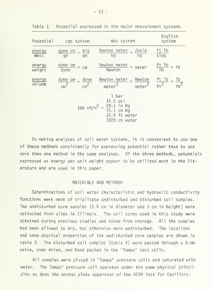
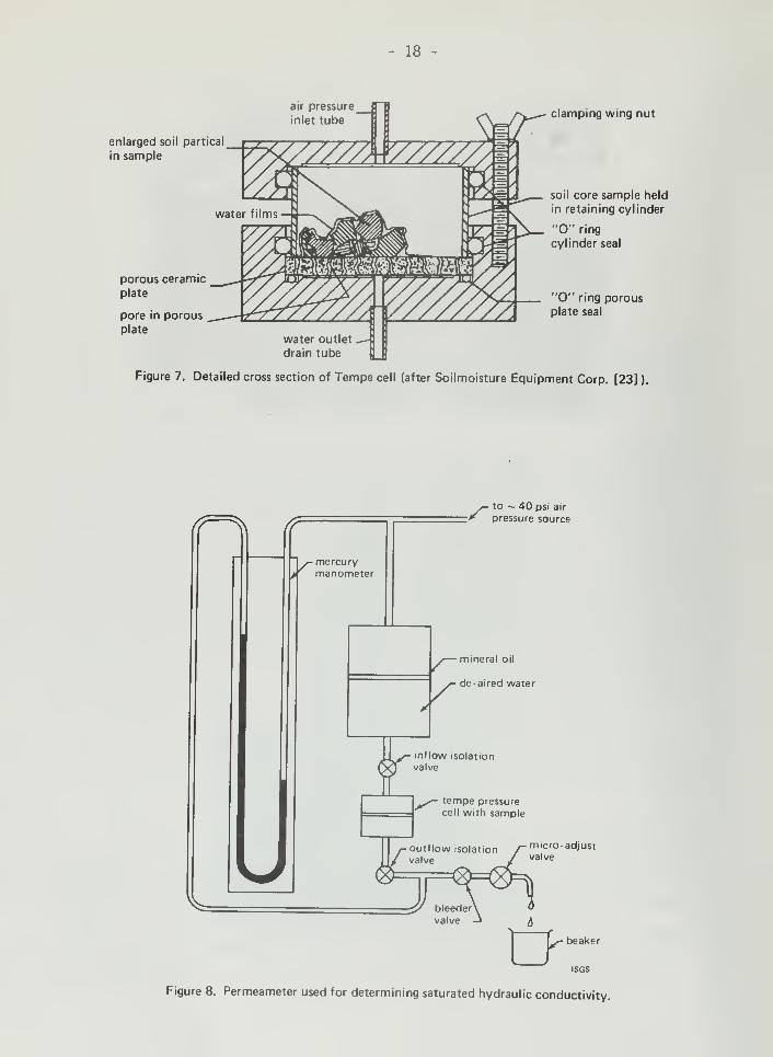
Figure 8. Permeameter used for determining saturated hydraulic conductivity.

- 19

calculate the hydraulic conductivities, using Equation 16 and the soil

water-retention curves.

The Lakeland fine sand samples were taken at three depth intervals

from the Agricultural Experiment Station farm of the University of Florida

at Quincy, Florida (Elzeftawy and Mansell {11}).

RESULTS

Amerman (14) and Philip (15) have pointed out the importance of includ-

ing information about the unsaturated soil properties in large-scale

hydrogeologic investigations. For example, to incorporate principles of

soil physics into a rainfall-runoff model, it is possible to use either a

numerical solution of the unsaturated flow equation or a simple infiltration

equation such as that given by Green and Ampt (16) or derived by Philip (17).

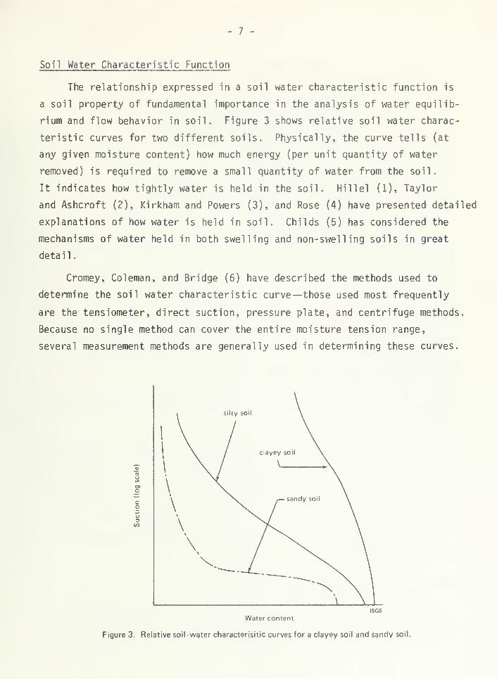
In the first approach, the soil water characteristic (the relationship

between soil suction head, h, and volumetric water content, e) and the

conductivity function (the relationship between the unsaturated hydraulic

conductivity K and e) must be known. In the second approach, composite

hydraulic parameters, specifically the Green-Ampt (16) wetting front suction,

h., and Philip (17) sorptivity, S, must be estimated or computed directly

from specified functions of h, K, and e.

The need to specify relationships among h, K, and e presents a signif-

icant problem in hydrology because of the difficulty of obtaining measure-

ments of these parameters and of presenting the collected data. Gardner,

et al. (18), Campbell (19), and Clapp and Hornberger (20) have attempted

to use power curves to describe the soil moisture characteristic of soils

and have had only limited success in estimating the hydraulic conductivities

from these power curves; however, Elzeftawy and Mansell (11) have shown

that the calculated hydraulic conductivity using Equation 16 provided a

good estimation of the K(e) function of Lakeland fine sand.

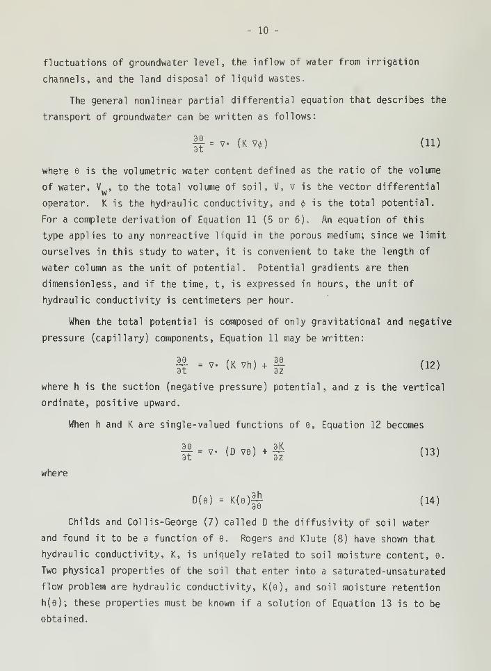
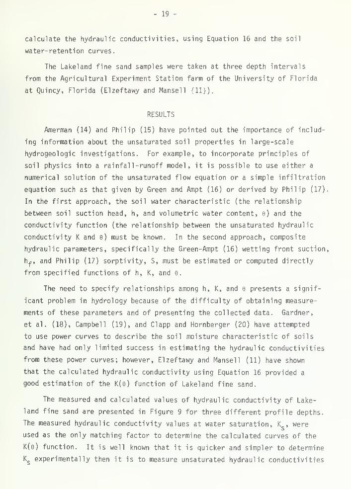
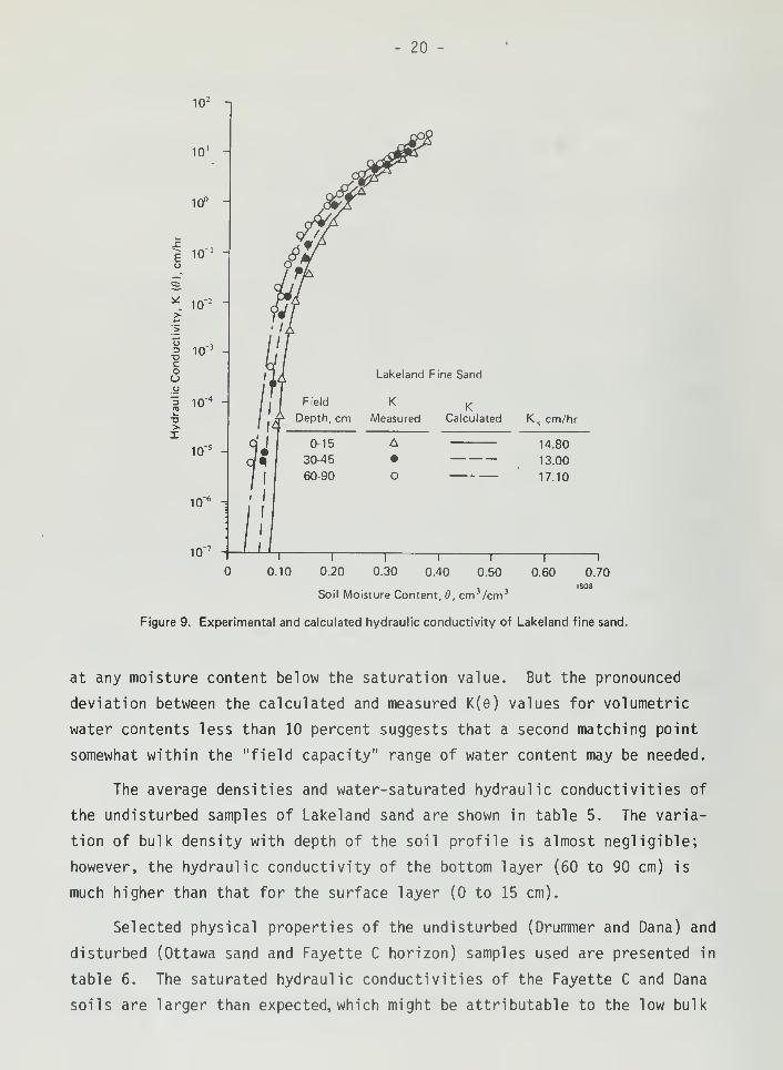
The measured and calculated values of hydraulic conductivity of Lake-

land fine sand are presented in Figure 9 for three different profile depths.

The measured hydraulic conductivity values at water saturation, K , were

used as the only matching factor to determine the calculated curves of the

K(e) function. It is well known that it is quicker and simpler to determine

Ksexperimentally then it is to measure unsaturated hydraulic conductivities

20 -

10 2-i

10' -

10"

10

* 10 2

% 10coO

£ 10

>I

10s

-

10~* -

10"

Lakeland Fine Sand

KCalculated K

scm/hr

14.80

13.00

17.10

1—

0.10

T 1

0.60 0.70ISGS

0.20 0.30 0.40 0.50

Soil Moisture Content, 6, cm 3 /cm 3

Figure 9. Experimental and calculated hydraulic conductivity of Lakeland fine sand.

at any moisture content below the saturation value. But the pronounced

deviation between the calculated and measured K(e) values for volumetric

water contents less than 10 percent suggests that a second matching point

somewhat within the "field capacity" range of water content may be needed.

The average densities and water-saturated hydraulic conductivities of

the undisturbed samples of Lakeland sand are shown in table 5. The varia-

tion of bulk density with depth of the soil profile is almost negligible;

however, the hydraulic conductivity of the bottom layer (60 to 90 cm) is

much higher than that for the surface layer (0 to 15 cm).

Selected physical properties of the undisturbed (Drummer and Dana) and

disturbed (Ottawa sand and Fayette C horizon) samples used are presented in

table 6. The saturated hydraulic conductivities of the Fayette C and Dana

soils are larger than expected, which might be attributable to the low bulk

- 21

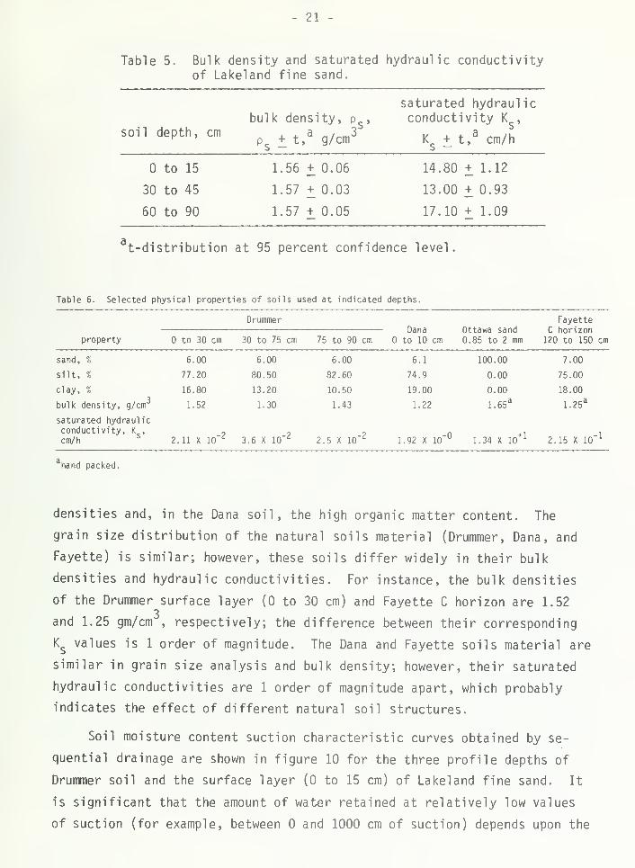
Table 5. Bulk density and saturated hydraulic conductivityof Lakeland fine sand.

saturated hydraulicbulk density, p , conductivity K ,

soil depth, cm , . a „/„„,3 v , . a „m/uKps

+ t, g/cm Ks

+ t, cm/h

to 15 1.56 + 0.06 14.80 + 1.12

30 to 45 1.57+0.03 13.00+0.93

60 to 90 1.57+0.05 17.10+1.09

at-distribution at 95 percent confidence level.

Table 6. Selected physical properties of soils used at indicated depths.

DrummerDana

to 10 cmOttawa sand

0.85 to 2 mm

FayetteC horizon120 to 150 cmproperty to 30 cm 30 to 75 cm 75 to 90 cm

sand, % 6.00 6.00 6.00 6.1 100.00 7.00

silt, % 77.20 80.50 82.60 74.9 0.00 75.00

clay, % 16.80 13.20 10.50 19.00 0.00 18.003

bulk density, g/cm 1.52 1.30 1.43 1.22 1.65a

1.25a

saturated hydraulicconductivity, K ,

cm/h 2,.11 X 10" 23.6 X 10" 2

2.5 X 10" 21.92 X 10"° 1.34 X 10

+12.15 X 10" 1

hand packed.

densities and, in the Dana soil, the high organic matter content. The

grain size distribution of the natural soils material (Drummer, Dana, and

Fayette) is similar; however, these soils differ widely in their bulk

densities and hydraulic conductivities. For instance, the bulk densities

of the Drummer surface layer (0 to 30 cm) and Fayette C horizon are 1.523

and 1.25 gm/cm , respectively; the difference between their corresponding

Ks

values is 1 order of magnitude. The Dana and Fayette soils material are

similar in grain size analysis and bulk density; however, their saturated

hydraulic conductivities are 1 order of magnitude apart, which probably

indicates the effect of different natural soil structures.

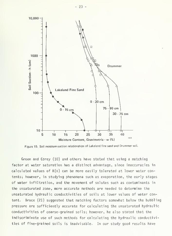
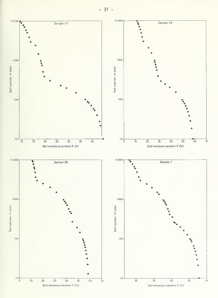
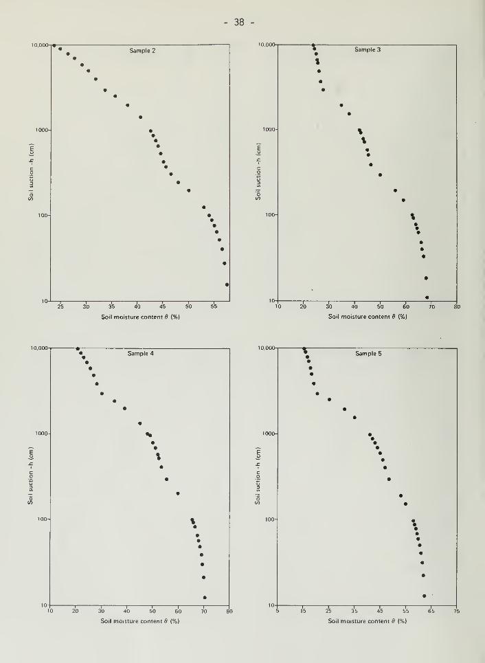
Soil moisture content suction characteristic curves obtained by se-

quential drainage are shown in figure 10 for the three profile depths of

Drummer soil and the surface layer (0 to 15 cm) of Lakeland fine sand. It

is significant that the amount of water retained at relatively low values

of suction (for example, between and 1000 cm of suction) depends upon the

- 22 -

capillary effect and the pore size distribution and therefore is strongly

affected by the soil structure. On the other hand, water retention in the

higher suction range is due increasingly to adsorption and is thus influenced

less by the structure and more by the texture and specific surface of the

soil material. Figure 10 indicates that, in general, the greater the clay

content, the greater the water content, at any particular suction (compare

Lakeland sand and Drummer silty loam) and the more gradual the slope of the

curve.

The effect of compaction upon a soil is to decrease its total porosity,

and especially to decrease the volume of the large interaggregate pores;

this means that water content at saturation and the initial decrease of

water content with the application of low suction are reduced. The data

presented in table 6 and figure 10 for the 30 to 75-cm and 75 to 90-cm depth

of Drummer samples support the previous statement: note the similarity in

their particle-size analysis and the differences in their bulk densities

and the saturated water contents.

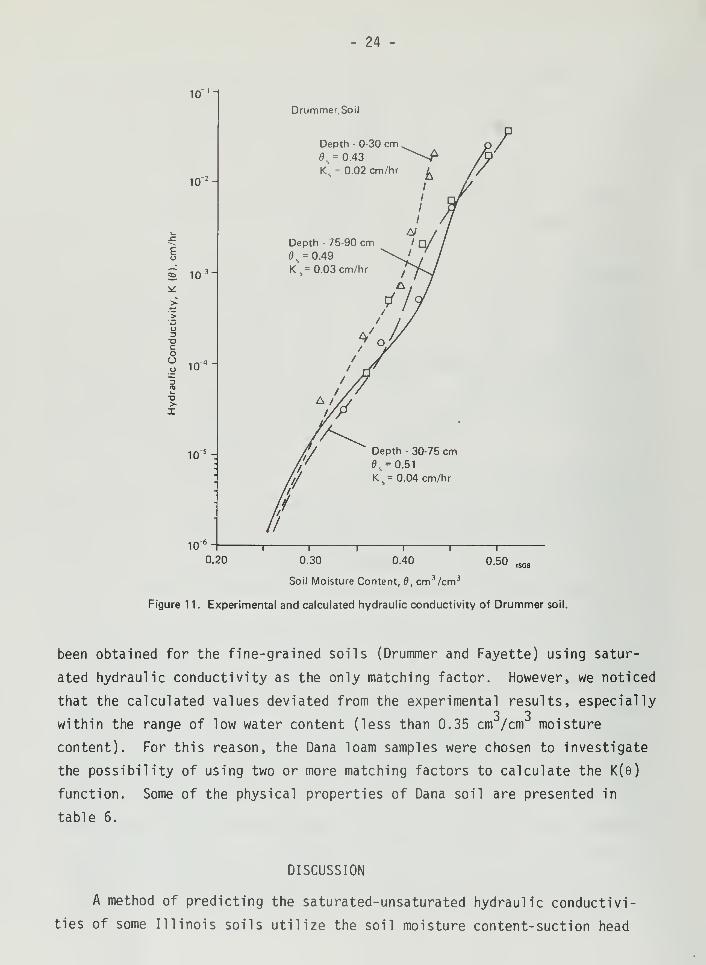
The calculated and experimental hydraulic conductivities of three lay-

ers of Drummer soil profiles are shown in figure 11. The experimental data

were obtained by the unit gradient method as published by Elzeftawy and

Mansell (12). The hydraulic conductivity of this soil at saturation is

generally about 4 orders of magnitude larger than at 50 percent of satura-

tion. The calculated results were consistent with the experimental data;3 3

however, the calculated numerical values below 0.32 cm /cm water content

were less than the experimentally hydraulic conductivities obtained (not

shown in figure 11).

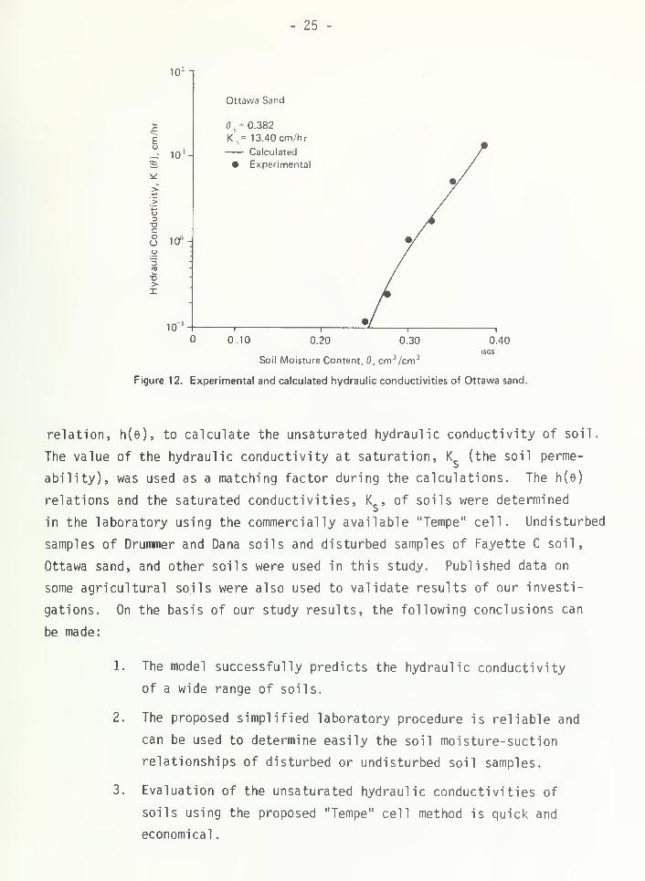
Hydraulic conductivities as a function of moisture content of Ottawa

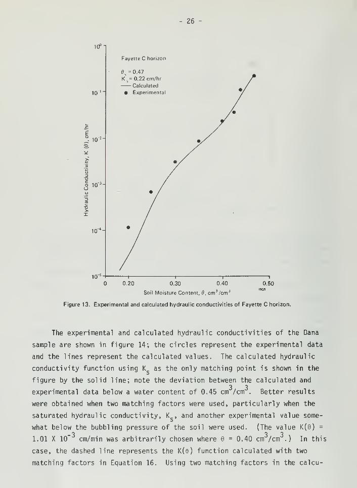
sand and Fayette C horizon are shown in figures 12 and 13. The lines repre-

sent the calculated values of K(e) obtained by Equation 16 and the soil-

moisture retention curve. The circles are the experimental data points.

These soil materials represent a wide range of pore size distributions over

which the calculations of hydraulic conductivities are based. Figure 13

3'

shows that a change in water content of Fayette soil from 0.47 to 0.30 cm /cm"

has reduced the hydraulic conductivity from 2.2 X 10_1

cm/h to 4.0 X 10" 3

cm/h, respectively.

- 23

10,000^1

1000

co'û300

'5

00

100-

10

Lakeland Fine Sand

0- 15 cm

Drummer

75 - 90 cm

30 - 75 cm

30*r

5 10 15 20 25 30 35 40

Moisture Content, Gravimetric - w (%)

Figure 10. Soil moisture-suction relationships of Lakeland fine sand and Drummer soil.

Green and Corey (10) and others have stated that using a matching

factor at water saturation has a distinct advantage, since inaccuracies in

calculated values of K(e) can be more easily tolerated at lower water con-

tents; however, in studying phenomena such as evaporation, the early stages

of water infiltration, and the movement of solutes such as contaminants in

the unsaturated zone, more accurate methods are needed to determine the

unsaturated hydraulic conductivities of soils at lower values of water con-

tent. Bruce (21) suggested that matching factors somewhat below the bubbling

pressure are sufficiently accurate for calculating the unsaturated hydraulic

conductivities of coarse-grained soils; however, he also stated that the

indiscriminate use of such methods for calculating the hydraulic conductivi-

ties of fine-grained soils is inadvisable. In our study good results have

- 24 -

10"

Eu

o3acoo

a>X

10"

10

10"

10-5 _

10"6-

0.20

Drummer, Soil

Depth • 0-30 cm

S= O.43 ^^£

Ks= 0.02 cm/hr ^

/

/

/

/

A/Depth - 75-90 cm / /

S= O.49

K = 0.03 cm/hr

Depth - 30-75 cm

,=0.51

Ks= 0.04 cm/hr

—I

—

0.30 0.500.40


Figure 11. Experimental and calculated hydraulic conductivity of Drummer soil

been obtained for the fine-grained soils (Drummer and Fayette) using satur-

ated hydraulic conductivity as the only matching factor. However, we noticed

that the calculated values deviated from the experimental results, especially3 3

within the range of low water content (less than 0.35 cm /cm moisture

content). For this reason, the Dana loam samples were chosen to investigate

the possibility of using two or more matching factors to calculate the K(e)

function. Some of the physical properties of Dana soil are presented in

table 6.

DISCUSSION

A method of predicting the saturated-unsaturated hydraulic conductivi-

ties of some Illinois soils utilize the soil moisture content-suction head

- 25

102

E" 10'2.

3gcoo

a>I

10°

10"

Ottawa Sand

0^=0.382K

b= 13.40 cm/hr

Calculated

• Experimental

0.40ISGS

0.10 0.20 0.30


Figure 12. Experimental and calculated hydraulic conductivities of Ottawa sand.

relation, h(e), to calculate the unsaturated hydraulic conductivity of soil.

The value of the hydraulic conductivity at saturation, K (the soil perme-

ability), was used as a matching factor during the calculations. The h(e)

relations and the saturated conductivities, K , of soils were determined

in the laboratory using the commercially available "Tempe" cell. Undisturbed

samples of Drummer and Dana soils and disturbed samples of Fayette C soil,

Ottawa sand, and other soils were used in this study. Published data on

some agricultural soils were also used to validate results of our investi-

gations. On the basis of our study results, the following conclusions can

be made:

1. The model successfully predicts the hydraulic conductivity

of a wide range of soils.

2. The proposed simplified laboratory procedure is reliable and

can be used to determine easily the soil moisture-suction

relationships of disturbed or undisturbed soil samples.

3. Evaluation of the unsaturated hydraulic conductivities of

soils using the proposed "Tempe" cell method is quick and

economical

.

- 26 -

10Pl

10

E-10"

3XI

| 10

a>I

3_

104 _

10"

Fayette C horizon

S=O.47

Ks=0.22cm/hr

Calculated

• Experimental

0.50ISGS

0.20 0.30 0.40


Figure 13. Experimental and calculated hydraulic conductivities of Fayette C horizon.

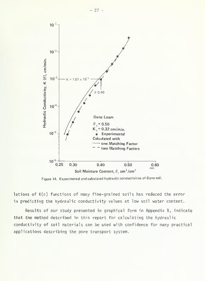
The experimental and calculated hydraulic conductivities of the Dana

sample are shown in figure 14; the circles represent the experimental data

and the lines represent the calculated values. The calculated hydraulic

conductivity function using K as the only matching point is shown in the

figure by the solid line; note the deviation between the calculated and3 3

experimental data below a water content of 0.45 cm /cm . Better results

were obtained when two matching factors were used, particularly when the

saturated hydraulic conductivity, K , and another experimental value some-

what below the bubbling pressure of the soil were used. (The value K(6) =

-3 3 31.01 X 10 cm/min was arbitrarily chosen where = 0.40 cm /cm .) In this

case, the dashed line represents the K(e) function calculated with two

matching factors in Equation 16. Using two matching factors in the calcu-

27 -

10i _,

I

"2-10

Eu

S 103

10

DO i n'4O

10s

-.

10-6

K = 1.01 x 10

Dana Loam

ds= 0.50

Ks= 0.32 cm/min.

• Experimental

Calculated with

one Matching Factor

two Matching Factors

0.25 0.60ISGS

0.30 0.40 0.50


Figure 14. Experimental and calculated hydraulic conductivities of Dana soi

lations of K(e) functions of many fine-grained soils has reduced the error

in predicting the hydraulic conductivity values at low soil water content.

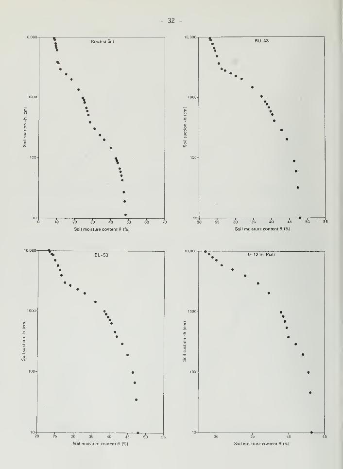
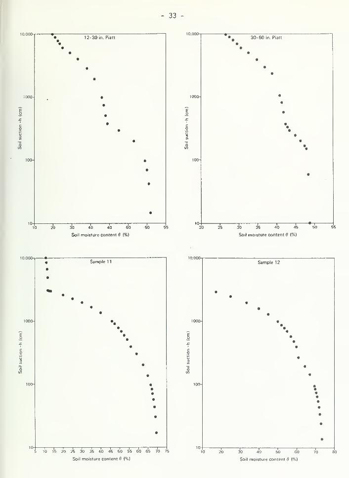
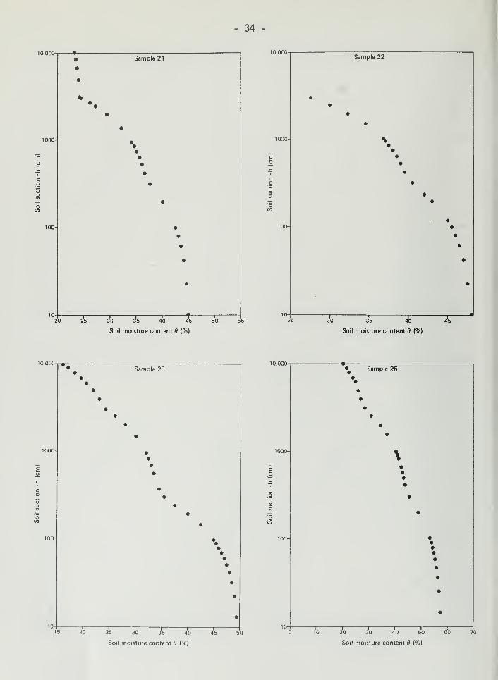
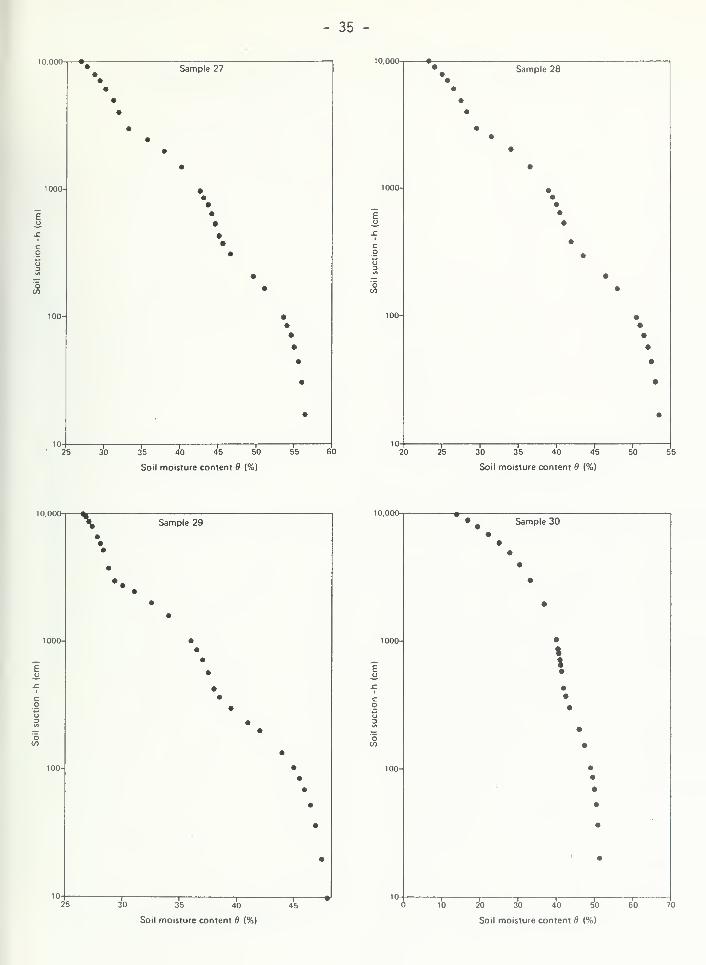
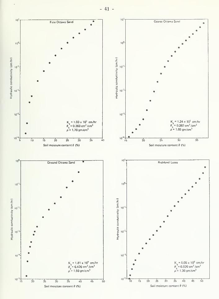
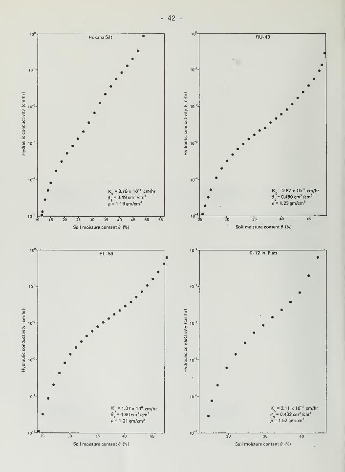
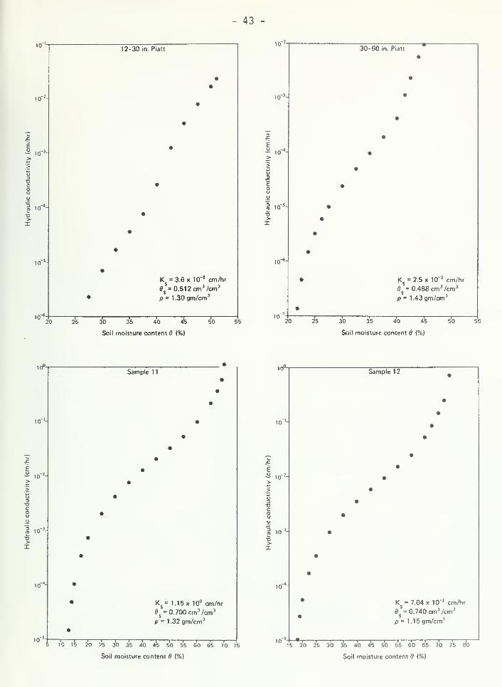
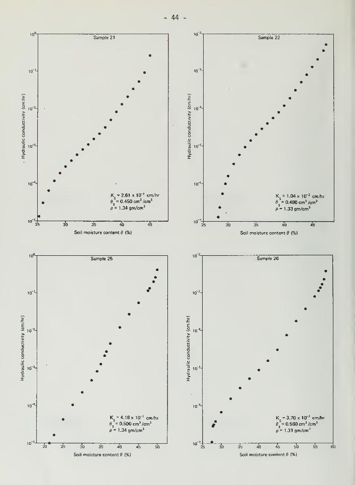
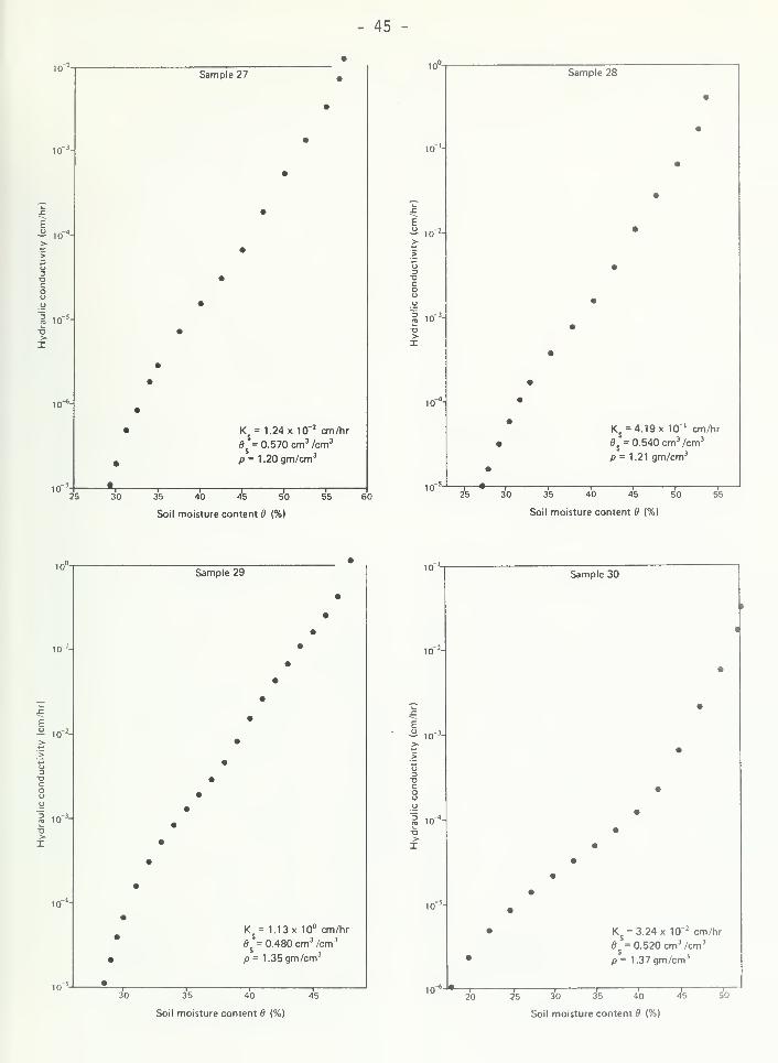
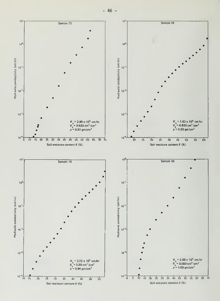
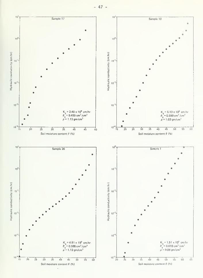
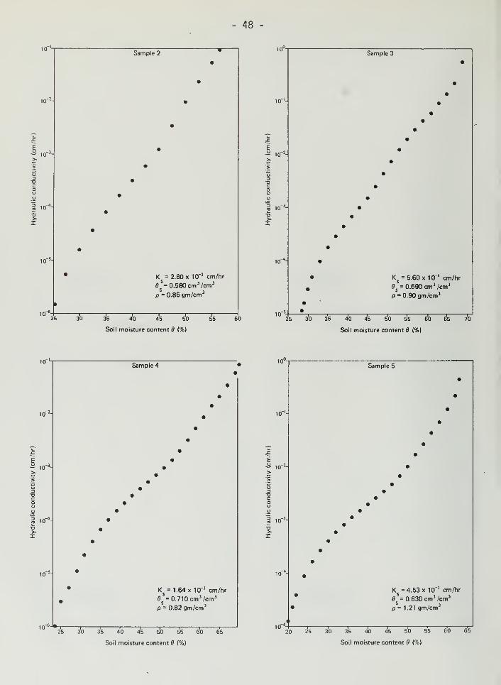
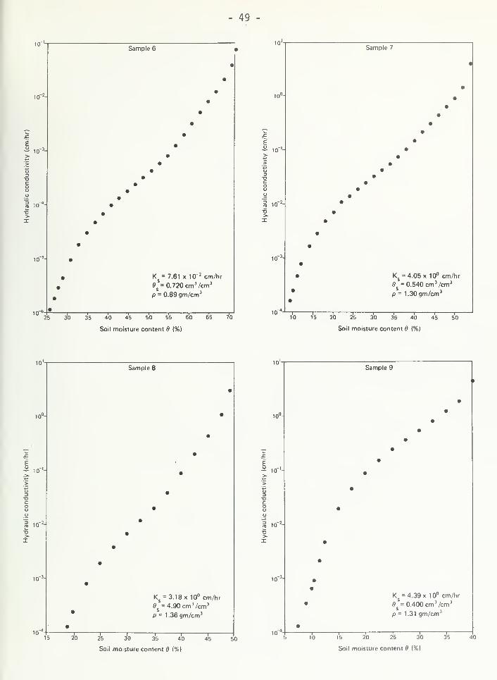
Results of our study presented in graphical form in Appendix B, indicate

that the method described in this report for calculating the hydraulic

conductivity of soil materials can be used with confidence for many practical

applications describing the pore transport system.

- 28 -

REFERENCES

1. Hi 1 lei , D. , Soil and Water, Physical Principles and Processes, AcademicPress, New York, 1973.

2. Taylor, S. A. and G. L. Ashcroft, Physical Edaphology, The Physics of

Irrigated and Nonirrigated Soils, W. H. Freeman and Company, San

Francisco, California, 1972.

3. Kirkham, D. and W. L. Powers, Advanced Soil Physics, John Wiley and

Sons, Inc., New York, 1972.

4. Rose, C. W., Agriculture Physics, Pergamon Press, New York, 1966.

5. Childs, E. C. , An Introduction to the Physical Basis of Soil WaterPhenomena, John Wiley and Sons, Inc., New York, 1969.

6. Cromey, D. , J. E. Coleman, and P. M. Bridge, Road Research Laboratory,Crowthorne, England, 1951.

7. Childs, E. C. and N. Collis-George, Proceedings of the Royal Societyof London, Vol. A, No. 2-1, 1950, pp. 392-405.

8. Rogers, J. S. and A. Klute, Soil Science Society of America, Proceed-ings, Vol. 35, 1971, pp. 695-700.

9. Millington, R. J. and J. R. Quirk, Transactions of the Faraday Society,Vol. 57, 1961, pp. 1200-1207.

10. Green, R. E. and J. C. Corey, Science Society of America, Proceedings,Vol. 35, 1971, pp. 3-8.

11. Elzeftawy, A. and R. S. Mansell, Soil Science Society of America,Proceedings, Vol. 39, 1975, pp. 599-603.

12. Elzeftawy, A. and B. J. Dempsey, Transportation Research Record, Vol.

642, pp. 30-35.

13. Watson, K. K. , Water Resources Research, Vol. 2, 1966, pp. 509-517.

14. Amerman, C. R. , Hydrology and Oil Science, SSSA Special PublicationsSeries, No. 5, Soil Science Society of America, Madison,Wisconsin, 1973.

15. Philip, J. R. , in Prediction in Catchment Hydrology, C. H. M. van Bauel

,

Ed., Australian Academy of Science, 1975, pp. 23-30.

16. Green, W. Heber and G. A. Ampt, Journal of Agricultural Science, Vol.

4, 1911, pp. 1-24.

17. Philip, J. R., Soil Science, Vol. 84, 1957, pp. 257-264.

18. Gardner, W. R. , D. Hi 1 1 el , and Y. Benyamini, Water Resources Research,Vol. 6, 1970, pp. 851-861.

- 29 -

19. Campbell, G. S., Soil Science, Vol. 117, 1974, pp. 311-314.

20. Clapp, R. B. and G. M. Hornberger, Water Resources Research, Vol.

14, 1978, pp. 601-614.

21. Bruce, R. R. , Soil Science Society of America, Proceedings, Vol. 36,

1972, pp. 555-561.

22. Dempsey, B. S. and A. Elzeftawy, Moisture Movement and MoistureMovement Equilibrium in Pavement Systems Univ. of IllinoisEngineering Experimental Station, Urbana, Illinois, UILU-ENG-76-2012, 1976, 147 p.

23. Soil Moisture Equipment Corp., Tempe Pressure Cell, CatalogNo. 1400, 8 p.

24. Follmer, L. R. , 1982, in Thorn, C. E. [ed.] Space and Time in

Geomorphology: The "Binghampton" Symposium in Geomorphology:International Series, no. 12, London: George Allen and Unwin,

p. 117-146.

25. McKay, E. D. , A. Elzeftawy and K. Cartwright, 1979, IllinoisGeological Survey, EGN No. 85, 32 p.

LIST OF PUBLICATIONS

1. Elzeftawy, Atef. 1979. Modeling the Transport of Heat, Water and

Solute in Unsaturated Soil and Earth Materials. ASAE Proceed-

ings of "Hydrologic Transport Modeling Symposium." American

Society of Agricultural Engineers, St. Joseph, Michigan, 49085.

P. 234-245.

2. Elzeftawy, Atef. 1979. Waste Disposal and Transport Phenomena in

Soil. Proceedings of the 2nd Annual Conference of Applied

Research and Practice on Municipal and Industrial Waste.

Madison, Wisconsin. P. 583-595.

3. Elzeftawy, Atef and Keros Cartwright. 1981. Evaluating the Saturated

and Unsaturated Hydraulic Conductivity of Soils. ASTM Special

Technical Publication (STP) 746, P. 168-181, Philadelphia,

Pennsylvania.

- 30 -

Appendix A

Soil-Moisture Characteristics of Samples Used in This Study.

- 31 -

10,000-

1000-

100-

10-

Fine Ottawa Sand

10 15 20 25

Soil moisture content 6 (%)

To" 35

10.000-

1000-

100-

1010

Coarse Ottawa Sand

~l

—

15—

r

-

20-r—30 35 40 45


10,000

1000-

10.000-

20 40 45 50


1000-

100-

10

"1"Richland Loess

10r20 30 60 70


- 32 -

lO.OOO-i

\Roxana Silt

100-

20 30 40 50

Soil moisture content ft (%)

10,000


10.000

1000- 1000-

30 35


50155


- 33 -

10.000

1000-

10.000-

1000-

100- 100

30-60 in. Piatt

20 25 30 35-1

—

40-•-I-

50 55

Soil moisture content 8 (%) Soil moisture content 6 (%)

10.000

1000

10.000

100-

1000-

Sample 12

-r—20

#.

-1

—

50

Soil moisture content (%)

30 40


-1

—

70 HO

34 -

10.000

1000-

10,000-

30 35 40 45


50 55

Sample 22

25-

T

-45


Sample 25

15 25T35

10.000

Soil moisture content f) (%)

20 30 40


- 35 -

Sample 27

1000-

100-

10-

25 30 35 40

—r~45 50

-1

—

55

10.000

1000-

60

100-


30 35 40


10,000

1000-

10.000-

100-

1000-

100

10


20 30 40 5(


60

- 36 -

Sample 13

1000-

100-

10 20 30 40 5(


ra

Sample 14

"~i

—

20 30 40 50 60 70


lO.OOOn

1000-

10-

Sample 15

20 30—I

—

40 50

Soil moisture content II (%)

« Sample 16

in 20 40 60 70

Soil moisture content 8 {%)

- 37

10.000

1000-

10.000

100-

1000

100

20 25 30 35

Soil moisture content (%) Soil moisture content 6 (%)

10.000

1000-

10.000

100-

40 50


60 70

100-

45 55


65

- 38 -

1000-

10.000-

1000-

10-

%

Sample 3

10 30—1

—

50 60 80

Soil moisture content 8 (%) Soil moisture content 8 (%)

10.000-,

Sample 4

1000-

20 4030 40 50


70

10.000

1000

80

100-

35 45 55


;•,

39 -

10.000-

1000-

100-

Sample 6

20~1

—

30~

r

-

40—I

—

50 60-1

—

70 80


1000-

i nn-

10

Sample 7

10 20 30 60 70


10.000

100-

10

10.000-

25 30 35 40


1000-

100

111

Sample 9

10 15 20 25 30


35

40 -

Appendix B

The hydraulic conductivity soil -moisture relationships forsamples used in this study. Note, the rewetting of dry samplesmay have increased the saturated hydraulic conductivity in

some samples.

- 41 -

10"

E3 m-M

10

10'

Fine Ottawa Sand

K = 1.03 x 10' cm/hr

= 0.363 cm 3 /cm 3

p = 1.70gm/cm3

10 15 20 25 30


35 40

10°

e-^ io-

io"--

10

10

Coarse Ottawa Sand

••

••

••

•

•

•

•

•

•

•

•

•

•

•K$= 1.34x10' cm/hr

•

••

S= 0.382 cm 3 /cm 3

p = 1.65 gm/cm 3

•1 ~ - T "

T-

1

20 25 30 35


10

E

10

Ground Ottawa Sand

K = 1.81 x 10° cm/hrS= 0.420 cm 3 /cm 3

p = 1.50 gm/cm 3

20 25 30 35 40


50

10'

E£ io-

10

10

Richland Loess

K =5.05x 10° cm/hr

d = 0.520 cm 3 /cm 3

p = 1.30 gm/cm 3

I 25 30 35 40


42

10°-

Roxana Silt •

•

•

•tcrL •

•

•

.c•

conductivity

(cm

o•

•

•

•

y

| io"3-

I

•

•

•

•

•

10"4-

•

• Ks= 8.76x 10"' cm/hr

# 8S= 0.49 cm 3 /cm3

p = 1.19gm/cm 3

10"S-

•i i i i i ii i i

10"

10 25 30 35 40 50

E2 io-M

10

10"

RU-43

25

Ks

= 2.87x10"' cm/hr

d%= 0.480 cm 3 /cm 3

p = 1 .23 gm/cm 3


30 35 40


to"

10

E^ 10"

10"

10"

10

EL-53

K$= 1.37 x 10° cm/hr

0,. = 4.80 cm 3 /cm 3

p = 1.21 gm/cm 3

25 30 35 40


10"

E£ io-

lO"

10"

0-12 in. Piatt

Ks

= 2.11 x 10" 2 cm/hr

8 =0.432 cm 3 /cm 3

p = 1.52 gm/cm 3

30 35


- 43 -

10

E5 ,0-3.

10

10

10"20

12-30 in. Piatt

K$= 3.6x10"' cm/hr

S= 0.512 cm 3 /cm 3

p = 1.30gm/cm 3

25 40 45 lo~ 55


10

10"

E-2 io-

10"

10H

10

30-60 in. Piatt

Ks= 2.5x 10" J cm/hr

S= 0.488 cm 3 /cm 3

/> = 1.43gm/cm 3

20 25 30 35 40 45


10'-

Ea 10

-3.

10

-a>I

10

10

Sample 11

Ks

-= 1.15 x 10° cm/hr

S= 0.700 cm 3

/cm 3

p= 1.32gm/cm 3

5 10 15 20 25 30 35 40 45 50 55 60 65 70 75


10°nSample 12

•

•10"'-

•

•

.c

£-H io"

2-

>>

•

•

•

•t>3TJcOU •

•

o

| 10" 3-

•o>I

•

•

•

10"4-

•

•

K =7.04x 10"' cm/hrS= 0.740 cm 3 /cm 3

p = 1.15 gm/cm 3

,„-s.101 5 20 25 3'0 35 40 45 50 55 6'0 65 70 75 80


- 44 -

10"

E

10-

Sample 21

K =2.61 x 10"' cm/hr

6 = 0.450 cm 3 /cm 3

p= 1.34gm/cm 3

30 35 40


45

10"

ES. io-

10

10'

1025

Sample 22

Ks= 1.04 x10"2 cm/hr

8i= 0.480 cm 3 /cm 3

p = 1 .33 gm/cm 3

35 40


iou-

Sample 25

•

••

10"L

•

jr

•

Hydraulic

conductivity

(cm

O

°i

•

•

•

••

•

•

•

10-"-

•

•

•

Ks= 4.18x10-' cm/hr

S= 0.500 cm 3

/cm3

p = 1 .34 gm/cm 3

,n-S-

10"

20 25 30 35 40 45


50

E2 10"'

10-

1025

Sample 26

Ks= 3.70x 10"' cm/hr

= 0.580 cm 3 /cm 3

p = 1.31 gm/cm3

35 40 45 50


60

- 45 -

10

10

E2 io-

10"

10"

1025

Sample 27

K$= 1.24 x 10~2 cm/hr

6 =0.570 cm 3 /cm3

p = 1.20gm/cm3

30 35 50 55 60

10 -

Sample 28

•

•

io-'-

•

X•

Hydraulic

conductivity

(err

•

•

•

•

•

•

10"4- •

•

•

Ks= 4.19x 10"' cm/hr

S= 0.540 cm 3 /cm3

p = 1.21 gm/cm 3

•

,r»-S_ A


25 30 35 40 45 50

Soil moisture content d (%)

1U~Sample 29

•

•

•

10"'- •

•

•

conductivity

(cm/hr)

o

•

•

•

•

•

•u

= in"J-ro 1U

•a>I

•

•

•

•

•

10"4 -

•

•

•

K = 1.13 x 10° cm/hr

$= 0.480 cm 3 /cm 3

p = 1.35 gm/cm 3

m-5. •

io"'-Sample 30

i

<

10" 2-

•

.c•

conductivity

(cm

•

•

o

| 10'4-

TJ>

•

•

•

•

•

•

10~ 5-

•

•

Ks

*5

= 3.24x 10~ 2 cm/hr

" 0.520 cm 3 /cm 3

,n-6- *-

• P = 1.37 gm/cm 3

30 35 40


45 20 30 40 50


- 46

10'

E5 10-'-

10

10*-

Sample 13

Ks= 3.90 x 10° cm/hr

8i= 0.620 cm 3

/cm 3

p = 0.91 gm/cm 3

10 15 20 25 30 35 40 45 50 55 60 65 70 75


I Of

ES io-'-I

10"

Sample 14

Ks=1.83x 10° cm/hr

s= 0.620 cm 3 /cm3

p = 0.92 gm/cm3

30 35 40 45 51


E& io-

10"

10

10'

Sample 15

Ks= 3.22x 10° cm/hr

S= 5.80 cm 3 /cm 3

p = 0.94 gm/cm3

15 20 25 30


10"

E^ io-

10

10

Sample 16

K$= 2.09x 10° cm/hr

9S= 0.600 cm 3 /cm 3

p = 1.00 gm/cm 3


47 -

10"-

£2 10"

10

10"

Sample 1 7

Ks= 2.40x10° cm/hr

s= 0.450 cm 3 /cm 3

p = 1.13gm/cm 3

10'

15 20-J—35>5 30 35 40


45 50

Sample 19

•

•

•

10°- ••

••

•_^ •X •E2 io-'-

•> •>

o •DDCo •uo

3 io"1- •

TJ,>-

X •

•

•10"3-

•

K =5.13x 10° cm/hr•

6 =0.590 cm 3 /cm 3

s

•p = 1 .03 gm/cm

10"4-—*-, , ,i i i i

15 20 30 35 40 50 60


io1

10"

E•H 10

-

Sample 20

Ks= 4.81 x 10° cm/hr

S= 0.590 cm 3 /cm 3

p = 1.12 gm/cm 3

10•4JL

30 35 55 60


10"

10"

E•= 10

L

io-

1020

Sample 1

K = 1.51 x 10° cm/hrS= 0.61 cm 3 /cm 3

p = 0.88 gm/cm 3

25 ~F -

r

-35 40

—r~45 50

-J—55 60


- 48 -

10

ES 10

-

io--

10'

Sampl S 2

•

•

2. •

•

S_

•

•

•

•

>_

•

•

s_

•

•

•

K =2.80x 10"' cm/hr

8 = 0.580 cm 3 /cm3

p = 0.86 gm/cm 3

2 5 3'0I

35i

40i i i

45 50 55 60

1U "

Sample 3

•

•

•10"'-

•

••

•

.c •

E •

> •>

o •3

c •oou •

3 io"3- •

> •I •

•

•

tcr»- •

• K$= 5.60x10"' cm/hr

• $= 0.690 cm 3 /cm 3

p = 0.90 gm/cm 3

•

10" 5H

•1 1 1 1 111!30 35 40 45 50 55 60

Soil moisture content 6 {%) Soil moisture content 6 (%)

10

ES 10" 3

10

10

10n

Sample 4

Ks= 1.64 x 10"' cm/hr

6%= 0.710 cm 3

/cm 3

p = 0.82 gm/cm 3

IT 35 40 50 60


10

Eo— 10

10

Sample 5

K =4.53x 10"' cm/hr

6 =0.630 cm 3 /cm 3

p = 1.21 gm/cm 3

30 35 40 45 50 55


65

- 49 -

10"

ES io~

3-

10 -

i or

Sample 6

K = 7.61 x 10" 2 cm/hr

0^=0.720 cm 3 /cm 3

p = 0.89 gm/cm 3

25 30 35 40 45 50 55 60 65 70


Sample 7

•

•

io°- •

•

•~•

.c

£ •

^ 10"'- •> •> •u •

D •C •oo •o •

3 10"2- •

o •>I

•

•

•

io"3-

•

•

•

•

Ks= 4.05x 10° cm/hr

S= 0.540 cm 3 /cm 3

p= 1.30 gm/cm 3

m-4-10 15 20 25 30 35 40 45 50


10'

10"

E^ 10"

io-l

r.

Sample 8

Ks= 3.18x 10° cm/hr

s= 4.9Ocm 3

/cm 3

p = 1.36 gm/cm 3

20—r—25 35 45 50


10'

10"

E3 io-

10

10"

10

Sample 9

Ks= 4.39x10° cm/hr

9 = 0.400 cm 3 /cm 3

s ,

p = 1.31 gm/cm

15 20 25 30


40

Date post:	11-Feb-2022
Category:	Documents
Upload:	others
View:	4 times
Download:	0 times

Undisturbed core method for determining and evaluating the - Ideals

Documents