Unequal pay or unequal employment?A cross-country analysis of gender gaps∗

Claudia OlivettiBoston University

Barbara PetrongoloLondon School of Economics

CEP, CEPR and IZA

January 2007

Abstract

Gender wage and employment gaps are negatively correlated across countries. We argue thatnon-random selection of women into work explains an important part of such correlation andthus of the observed variation in wage gaps. The idea is that, if women who are employed tend tohave relatively high-wage characteristics, low female employment rates may become consistentwith low gender wage gaps simply because low-wage women would not feature in the observedwage distribution. We explore this idea across the US and EU countries estimating gender gapsin potential wages. We recover information on wages for those not in work in a given year usingalternative imputation techniques. Imputation is based on (i) wage observations from otherwaves in the sample, (ii) observable characteristics of the nonemployed and (iii) a statisticalrepeated-sampling model. We then estimate median wage gaps on the resulting imputed wagedistributions, simply requiring assumptions on the position of the imputed wage observationswith respect to the median, but not on their level. We obtain higher median wage gaps onimputed rather than actual wage distributions for most countries in the sample. However, thisdifference is small in the US, the UK and most central and northern EU countries, and becomessizeable in Ireland, France and southern EU, all countries in which gender employment gapsare high. In particular, correction for employment selection explains more than a half of theobserved correlation between wage and employment gaps.Keywords: median gender gaps, sample selection, wage imputation.JEL classification: E24, J16, J31

∗We wish to thank Richard Blundell, Richard Freeman, Larry Katz, Kevin Lang, Alan Manning and StevePischke for their suggestions on earlier versions of this paper. We also acknowledge comments from seminars atseveral institutions, as well as from presentations at the Bank of Portugal Annual Conference 2005, the SOLE/EALEConference 2005, the Conference in Honor of Reuben Gronau 2005 and the NBER Summer Institute 2006 for veryuseful comments. Olivetti aknowledges the Radcliffe Institute for Advanced Studies for financial support. Petrongoloaknowledges the ESRC for financial support to the Centre for Economic Performance.

1

1 Introduction

There is substantial international variation in gender pay gaps, from 25-30 log points in the US and

the UK, to 10-20 log points in a number of central and northern European countries, down to an

average of 10 log points in southern Europe. International differences in overall wage dispersion are

typically found to play a role in explaining the variation in gender pay gaps (Blau and Kahn 1996,

2003). The idea is that a given level of dissimilarities between the characteristics of working men

and women translates into a higher gender wage gap the higher the overall level of wage inequality.

However, OECD (2002, chart 2.7) shows that, while differences in the wage structure do explain an

important portion of the international variation in gender wage gaps, the inequality-adjusted wage

gap in southern Europe remains substantially lower than in the rest of Europe and in the US.

In this paper we argue that, besides differences in wage inequality and therefore in the returns

associated to characteristics of working men and women, a significant portion of the international

variation in gender wage gaps may be explained by differences in characteristics themselves, whether

observed or unobserved. This idea is supported by the striking international variation in employ-

ment gaps, ranging from 10 percentage points in the US, UK and Scandinavian countries, to 15-25

points in northern and central Europe, up to 30-40 points in southern Europe and Ireland. If

selection into employment is non-random, it makes sense to worry about the way in which selection

may affect the resulting gender wage gap. In particular, if women who are employed tend to have

relatively high-wage characteristics, low female employment rates may become consistent with low

gender wage gaps simply because low-wage women would not feature in the observed wage distrib-

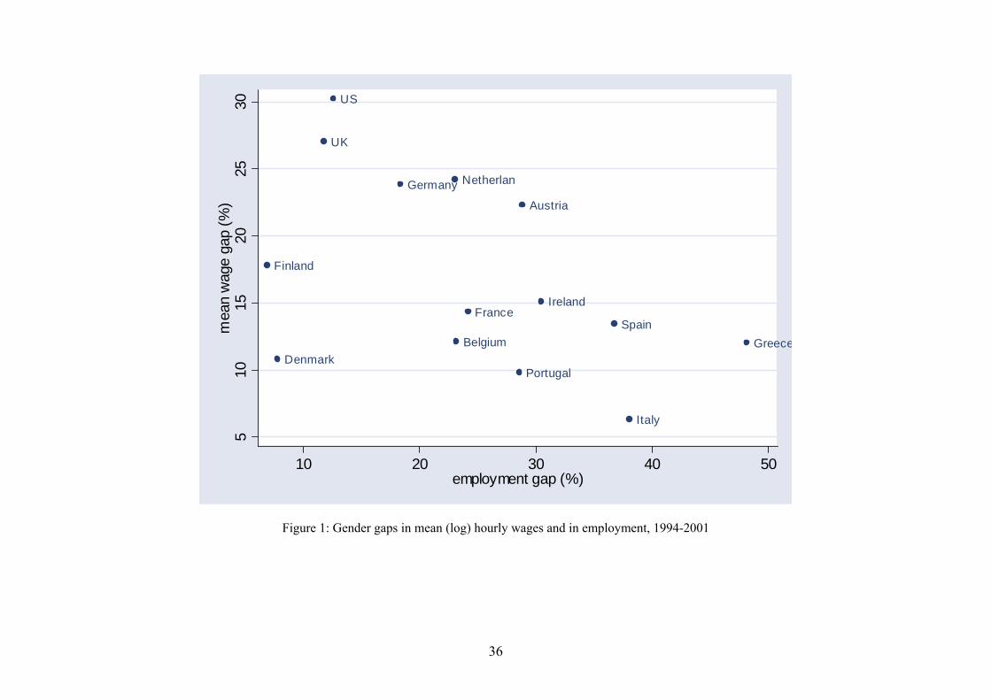
ution. This idea could thus be well suited to explain the negative correlation between gender wage

and employment gaps that we observe in the data (see Figure 1).

Different patterns of employment selection across countries may in turn stem from a number

of factors. First, there may be international differences in labor supply behavior and in particular

in the role of household composition and/or social norms in affecting participation. Second, labor

demand mechanisms, including social attitudes towards female employment and their potential

effects on employer choices, may be at work, affecting both the arrival rate and the level of wage

offers of the two genders. Finally, institutional differences in labor markets regarding unionization

and minimum wages may truncate the wage distribution at different points in different countries,

affecting both the composition of employment and the observed wage distribution. In this paper

we will be agnostic as regards the separate role of these factors in shaping gender gaps, and aim at

recovering alternative measures of selection-corrected gender wage gaps.

2

Although there exist substantial literatures on gender wage gaps on one hand, and gender

employment, unemployment and participation gaps on the other hand,1 to our knowledge the

variation in both quantities and prices in the labor market has not been simultaneously exploited

to understand important differences in gender gaps across countries. In this paper we claim that the

international variation in gender employment gaps can indeed shed some light on well-known cross-

country differences in gender wage gaps. We will explore this view by estimating selection-corrected

wage gaps.

In our empirical analysis we aim at recovering the counterfactual wage distribution that would

prevail in the absence of non-random selection into work - or at least some of its characteristics.

In order to do this, we recover information on wages for those not in work in a given year using

alternative imputation techniques. Our approach is closely related to that of Johnson, Kitamura

and Neal (2000) and Neal (2004), and simply requires assumptions on the position of the imputed

wage observations with respect to the median. Importantly, it does not require assumptions on

the actual level of missing wages, as typically required in the matching approach, nor it requires

arbitrary exclusion restrictions often invoked in two-stage Heckman sample selection correction

models.

We then estimate raw median wage gaps on the sample of employed workers (our base sample)

and on a sample enlarged with wage imputation for the nonemployed, in which selection issues are

alleviated. The impact of selection into work on estimated wage gaps is assessed by comparing

estimates obtained under alternative sample inclusion rules. The attractive feature of median re-

gressions is that, if missing wage observations fall completely on one or the other side of the median

regression line, the results are only affected by the position of wage observations with respect to

the median, and not by specific values of imputed wages. One can therefore make assumptions

motivated by economic theory on whether an individual who is not in work should have a wage

observation below or above median wages for their gender.

Imputation can be performed in several ways. Alternative imputation methods will address

slightly different economic mechanisms of selection, as will be described below. First, we use panel

data and, for all those not in work in some base year, we search backward and forward to recover

hourly wage observations from the nearest wave in the sample. This implicitly assumes that an

individual’s position with respect to the base-year median can be signalled by her wage from the

nearest wave. As imputation is simply driven by wages observed in other waves, we are in practice

1See Altonji and Blank (1999) for an overall survey on both employment and gender gaps for the US, Blauand Kahn (2003) for international comparisons of gender wage gaps and Azmat, Güell and Manning (2006) forinternational comparisons of unemployment gaps.

3

allowing for selection on unobservables. Estimates based on this procedure tell what level of the

gender wage gap we would observe if the nonemployed earned “similar” wages to those earned when

they were employed, where “similar” here means on the same side of the base-year median.

While our first imputation method arguably uses the minimum set of potentially arbitrary

assumptions, it has the disadvantage of not providing any wage information on individuals who

never work during the sample period. In order to recover wage observations also for those never

observed in work, we use economic insights to make educated guesses concerning their position with

respect to the median, based on their observable characteristics, specifically unemployment status,

education, experience and spouse income. In this case we are allowing for selection on observable

characteristics only, assuming that the nonemployed would earn wages “similar” to the wages of the

employed with matching characteristics, where again “similar” simply means on the same side of

the base-year median. Having done this, earlier or later wage observations for those with imputed

wages in the base year can shed light on the goodness of our imputation methods.

Finally, we extend the framework of Johnson et al. (2000) and Neal (2004) by using probability

models for assigning individuals on either side of the median of the wage distribution. We first esti-

mate the probability of each individual belonging above or below their gender-specific median using

a simple human capital specification. Individuals are then assigned above- or below-median wages

according to such predicted probabilities, using repeated imputation techniques (Rubin, 1987).

More specifically, the missing wage values are replaced by (a small number of) simulated versions,

thus obtaining independent simulated datasets. The estimated wage gaps on each of the simulated

complete datasets are combined to produce estimates and confidence intervals that incorporate

missing-data uncertainty. This method has the advantage of using all available information on the

characteristics of the nonemployed and of taking into account uncertainty about the reason for

missing wage information.

In our study we use panel data sets that are as comparable as possible across countries, namely

the Panel Study of Income Dynamics (PSID) for the US and the European Community Household

Panel Survey (ECHPS) for Europe. We consider the period 1994-2001, the longest time span for

which data are available for all countries. Our estimates on these data deliver higher median wage

gaps on imputed rather than actual wage distributions for most countries in the sample, and across

alternative imputation methods. This implies, as one would have expected, that women tend on

average to be more positively selected into work than men. However, the difference between actual

and potential wage gaps is small in the US, the UK and most central and northern European

countries, and becomes sizeable in Ireland, France and southern Europe, i.e. countries in which

4

the gender employment gap is highest. In other words, correcting for selection into employment

explains more than half of the observed negative correlation between gender wage and employment

gaps. In particular, in Spain, Italy, Portugal and Greece the median wage gap on the imputed wage

distribution reaches closely comparable levels to those of the US and of other central and northern

European countries.

Our results thus show that, while the raw wage gap is much higher in Anglo Saxon countries than

in Ireland and southern Europe, the reason is probably not to be found in more equal pay treatment

for women in the latter group of countries, but mainly in a different process of selection into

employment. Female participation rates in catholic countries and Greece are low and concentrated

among high-wage women. Having corrected for lower participation rates, the wage gap there widens

to similar levels to those of other European countries and the US.

The paper is organized as follows. Section 2 briefly discusses the related literature. Section 3

describes the data sets used and presents descriptive evidence on gender gaps. Section 4 describes

our imputation and estimation methodologies. Section 5 estimates raw median gender wage gaps

on actual and imputed wage distributions, to illustrate how alternative sample selection rules affect

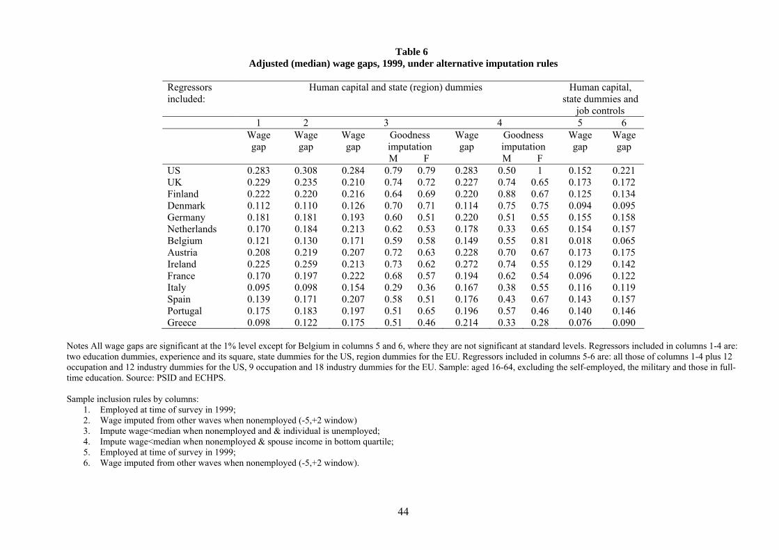
the estimated gaps. Section 6 looks at wage gaps corrected for characteristics. Section 7 studies

the relative contribution of employment selection versus wage dispersion in explaining the observed

variation in pay gaps. Conclusions are brought together in Section 8.

2 Related work

The importance of selectivity biases in making wage comparisons has long been recognized since

seminal work by Gronau (1974) and Heckman (1974). The current literature contains a number of

country-level studies that estimate selection-corrected wage gaps across genders or ethnic groups,

based on a variety of correction methodologies. Among studies that are more closely related to our

paper, Neal (2004) estimates the gap in potential earnings between black and white women in the

US by fitting median regressions on imputed wage distributions, using alternative methods of wage

imputation for women non employed in 1990. He finds that gap between potential earnings of white

and black women is at least 60 percent higher than the gap in actual earnings, thus revealing that

black women are more strongly selected into work according to high-wage characteristics. Using

both wage imputation and matching techniques, Chandra (2003) finds that the wage gap between

black and white US males was also understated, due to selective withdrawal of black men from the

5

labor force during the 1970s and 1980s.2

Turning to gender wage gaps, Blau and Kahn (2006) study changes in the US gender wage gap

between 1979 and 1998 and find that sample selection implies that the 1980s gains in women’s

relative wage offers were overstated, and that selection may also explain part of the slowdown

in convergence between male and female wages in the 1990s. Their approach is based on wage

imputation for those not in work, along the lines of Neal (2004). Mulligan and Rubinstein (2005)

also argue that the narrowing of the gender wage gap in the US during 1975-2001 may be a direct

impact of progressive selection into employment of high-wage women, in turn attracted by widening

within-gender wage dispersion. Correction for selection into work is implemented here using a two-

stage Heckman (1979) selection model. The authors show that while in the 1970s the gender

selection bias was negative, i.e. nonemployed women had higher earnings potential than working

women, it became positive in the mid 1980s.3

Related work on European countries includes Blundell, Gosling, Ichimura and Meghir (2007),

Albrecht, van Vuuren and Vroman (2004) and Beblo, Beninger, Heinze and Laisney (2003). Blundell

et al. examine changes in the distribution of wages in the UK during 1978-2000. They allow for the

impact of non-random selection into work by using bounds to the latent wage distribution according

to the procedure proposed by Manski (1994). Bounds are first constructed based on the worst case

scenario and then progressively tightened using restrictions motivated by economic theory. Features

of the resulting wage distribution are then analyzed, including overall wage inequality, returns to

education, and gender wage gaps. Albrecht et al. estimate gender wage gaps in the Netherlands

having corrected for selection of women into market work according to the Buchinsky’s (1998)

semi-parametric method for quantile regressions. They find evidence of strong positive selection

into full-time employment. Finally, Beblo et al. show selection corrected wage gaps for Germany

using both the Heckman (1979) and the Lewbel (2007) two-stage selection models. They find that

correction for selection has an ambiguous impact on gender wage gaps in Germany, depending on

the method used.

Interestingly, most studies find that correction for selection has important consequences for our

assessment of gender wage gaps. At the same time, none of these studies use data for southern

European countries, where employment rates of women are lowest, and thus the selection issue

should be most relevant. In this paper we use data for the US and for a representative group

2See also Blau and Beller (1992) and Juhn (2003) for earlier use of matching techniques in the study of selection-corrected race gaps.

3Earlier studies that discuss the importance of changing characteristics of the female workforce in explaining thedynamics of the gender wage gap in the US include O’Neil (1985), Smith and Ward (1989) and Goldin (1990).

6

of European countries to investigate how non-random selection into work may have affected the

gender wage gap.

3 Data

3.1 The PSID

Our analysis for the US is based on the Michigan Panel Study of Income Dynamics (PSID). This

is a longitudinal survey of a representative sample of US individuals and their households. It has

been ongoing since 1968. The data were collected annually through 1997 and every other year after

1997. In order to ensure consistency with European data, we use six waves from the PSID, from

1994 to 2001. We restrict our analysis to individuals aged 16-64, having excluded the self-employed,

full-time students, and individuals in the armed forces.4

The wage concept that we use throughout the analysis is the gross hourly wage. This is given

by annual labor income divided by annual hours worked in the calendar year before the interview

date. Employed workers are defined as those with positive hours worked in the previous year.

The characteristics that we exploit for wage imputation for the nonemployed are human capital

variables, spouse income and nonemployment status, i.e. unemployed versus out of the labor force.

Human capital is proxied by education and work experience controls. Ethnic origin is not included

here as information on ethnicity is not available for the European sample. We consider three broad

educational categories: less than high school, high school completed, and college completed. They

include individuals who have completed less than twelve years of schooling, between twelve and

fifteen years of schooling, and at least sixteen years of schooling, respectively. This categorization

of the years of schooling variable is chosen for consistency with the definition of education in the

ECHPS, which does not provide information on completed years of schooling, but only on recognized

qualifications.

Information on work experience refers to years of actual labor market experience (either full-

or part-time) since the age of 18. When individuals first join the PSID sample as a head or a wife

(or cohabitor), they are asked how many years they worked since age 18, and how many of these

years involved full-time work. These two questions are also asked retrospectively in 1974 and 1985,

irrespective of the year in which they had joined the sample. The answers to these questions are

4The exclusion of self-employed individuals may require some justification, in so far the incidence of self employmentvaries importantly across genders and countries, as well as the associated earnings gap. However, the availabledefinition of income for the self employed is not comparable to the one we are using for the employees and thenumber of observations for the self employed is very limited for European countries. Both these factors prevent usfrom including the self-employed in our analysis.

7

used to calculate actual work experience, following the procedure of Blau and Kahn (2006). Given

the initial values reported, we update work experience information for the years of interest using

the longitudinal work history file from the PSID. For example, in order to construct the years of

actual experience in 1994 for an individual who was in the survey in 1985, we add to the number of

years of experience reported in 1985 the number of years between 1985 and 1994 during which they

worked a positive number of hours.5 This procedure allows us to construct the full work experience

in each year until 1997. As the survey became biannual after 1997, there is no information on the

number of hours worked by individuals between 1997 and 1998 and between 1999 and 2000. We fill

missing work experience information for 1998 following again Blau and Kahn (2006). In particular,

we use the 1999 sample to estimate logit models for positive hours in the previous year and in

the year preceding the 1997 survey, separately for males and females. The explanatory variables

are race, schooling, experience, a marital status indicator and variables for the number of children

aged 0-2, 3-5, 6-10, and 11-15, who are living in the household at the time of the interview. Work

experience in the missing year is obtained as the average of the predicted values in the 1999 logit

and the 1997 logit. We repeat the same steps for filling missing work experience information in

2000.

Spouse income is constructed as the sum of total labor and business income in unincorporated

enterprises both for spouses and cohabitors of respondents. Finally, the reason for nonemployment,

i.e. unemployment versus inactivity, is given by self-reported information on employment status.

When estimating wage gaps adjusted for characteristics, we control for human capital and

job attributes. In particular, our wage equation includes controls for education, work experience,

industry and occupation. We consider 12 occupational categories, based on the 3-digits occupation

codes from the 1970 Census of the Population, and 12 industries. We also include 51 state dummies.

The results obtained on this specification were not sensitive to the inclusion of controls for ethnic

origin.

3.2 The ECHPS

Data for European countries are drawn from the European Community Household Panel Survey.

This is an unbalanced household-based panel survey, containing annual information on a few thou-

sands households per country during the period 1994-2001.6 The ECHPS has the advantage that

5The measure of actual experience used here includes both full-time and part-time work experience, as this isbetter comparable to the measure of experience available from the ECHPS.

6The initial sample sizes are as follows. Austria: 3,380; Belgium: 3490; Denmark: 3,482; Finland: 4,139; France:7,344; Germany: 11,175; Greece: 5,523; Ireland: 4,048; Italy: 7,115; Luxembourg: 1,011; Netherlands: 5,187;Portugal: 4,881; Spain: 7,206; Sweden: 5,891; U.K.: 10,905. These figures are the number of household included in

8

it asks a consistent set of questions across the 15 members states of the pre-enlargement EU. The

Employment section of the survey contains information on the jobs held by members of selected

households, including wages and hours of work. The household section allows to obtain information

on the family composition of respondents. We exclude Sweden and Luxembourg from our country

set, as wage information is unavailable for Sweden in all waves, and unavailable for Luxembourg

after 1996.

As for the US, we restrict our analysis of wages to individuals aged 16-64 as of the survey date,

and exclude the self-employed, those in full-time education and the military. The definition of

variables used replicates quite closely that used for the US.

Hourly wages are computed as gross weekly wages divided by weekly usual working hours.

The education categories used are: less than upper secondary high school, upper secondary school

completed, and higher education. These correspond to ISCED 0-2, 3, and 5-7, respectively. Unfor-

tunately, no information on actual experience is available in the ECHPS, and we use a measure of

potential work experience, computed as the current age of an individual, minus the age at which

she started her working life. Spouse income is computed as the sum of labor and non-labor annual

income for spouses or cohabitors of respondents. Finally, unemployment status is determined using

self-reported information on the main activity status.

When estimating adjusted wage gaps, our wage equation specification is as close as possible to

that estimated for the US, subject to slight data differences. Besides differences in the definition

for work experience, the occupational and industrial classification of individuals is slightly different

from the one used for the PSID. In particular, we consider 18 industries and 9 broad occupational

groups; although this is not the finest occupational disaggregation available in the ECHPS, it is

the one that allows the best match with the occupational classification available in the PSID. We

finally control for region of residence at the NUT1 level, meaning 11 regions for the UK, 1 for

Finland and Denmark, 15 for Germany, 1 for the Netherlands, 3 for Belgium and Austria, 2 for

Ireland, 8 for France, 12 for Italy, 7 for Spain, 2 for Portugal and 4 for Greece.

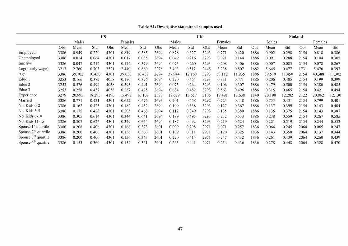
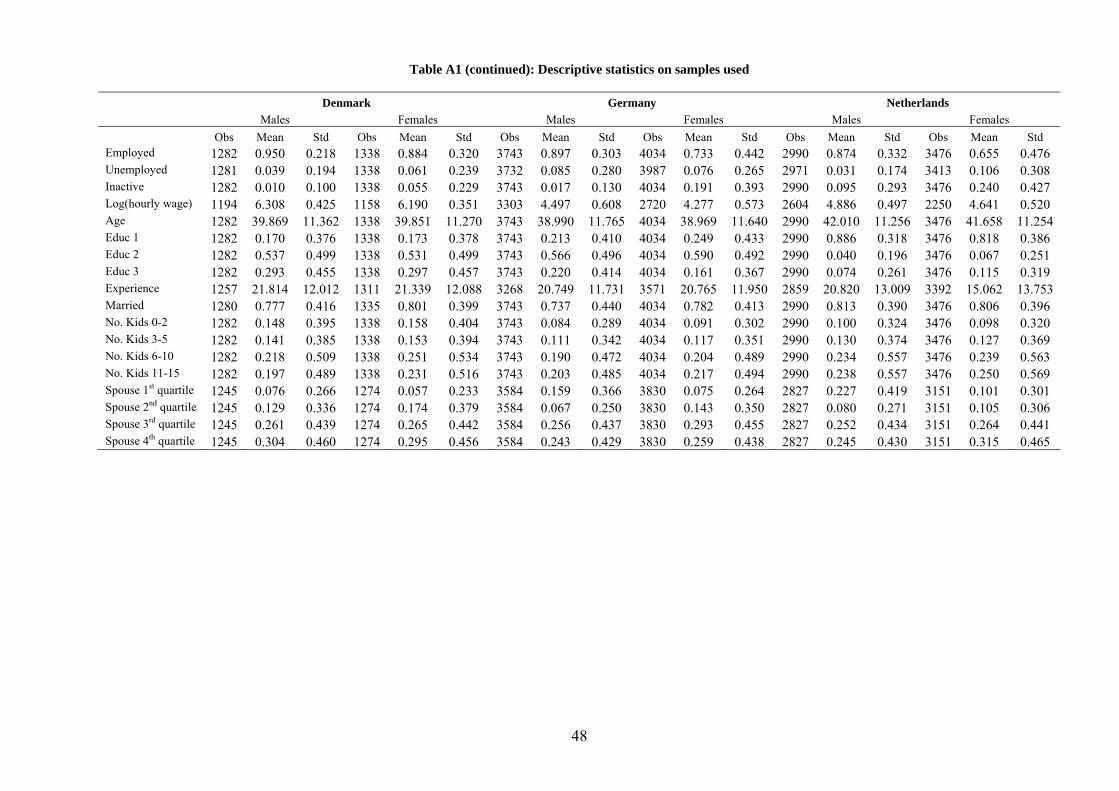
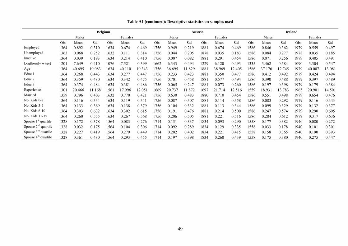
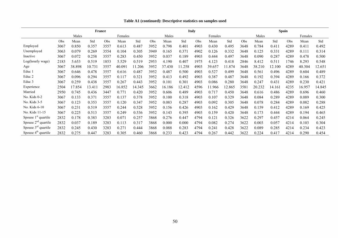
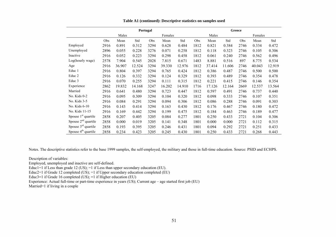
Descriptive statistics for both the US and the EU samples are reported in Table A1.

3.3 Descriptive evidence on gender gaps

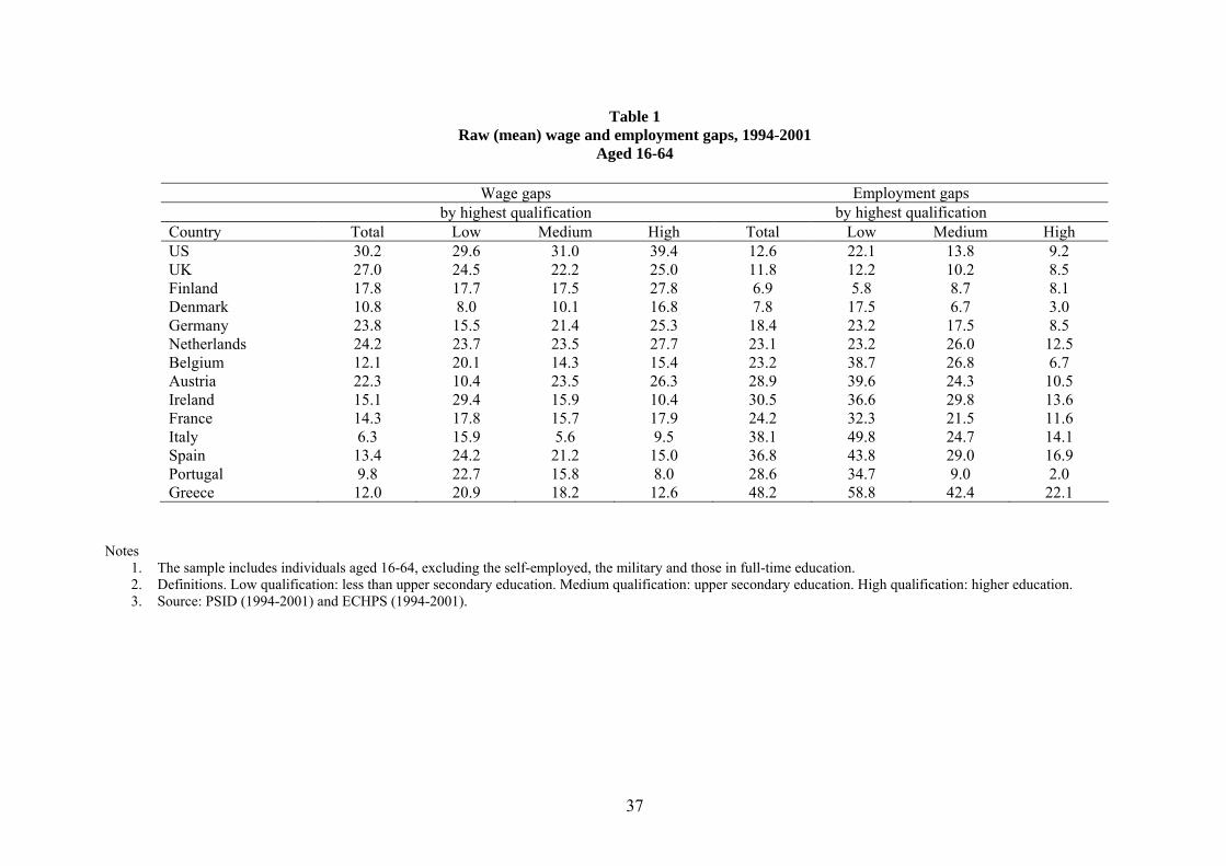
Table 1 reports raw gender gaps in log gross hourly wages and employment rates for all countries

in our sample. At the risk of some oversimplification, one can classify countries in three broad

the first wave for each country, which corresponds to 1995 for Austria, 1996 for Finland, 1997 for Sweden, and 1994for all other countries.

9

categories according to their levels of gender wage gaps. In the US and the UK men’s hourly wages

are 25 to 30 log points higher than women’s hourly wages. Next, in northern and central Europe the

gender wage gap in hourly wages is between 10 and 20 log points, from a minimum of 11 log points

in Denmark, to a maximum of 24 log points in the Netherlands. Finally, in southern European

countries the gender wage gap is on average 10 log points, from 6.3 in Italy to 13.4 in Spain. Such

gaps in hourly wages display a roughly negative correlation with gaps in employment to population

rates. Employment gaps range from 10 percentage points in the US, the UK and Scandinavia,7 to

15-25 points in northern and central Europe, up to 30-40 points in southern Europe and Ireland.

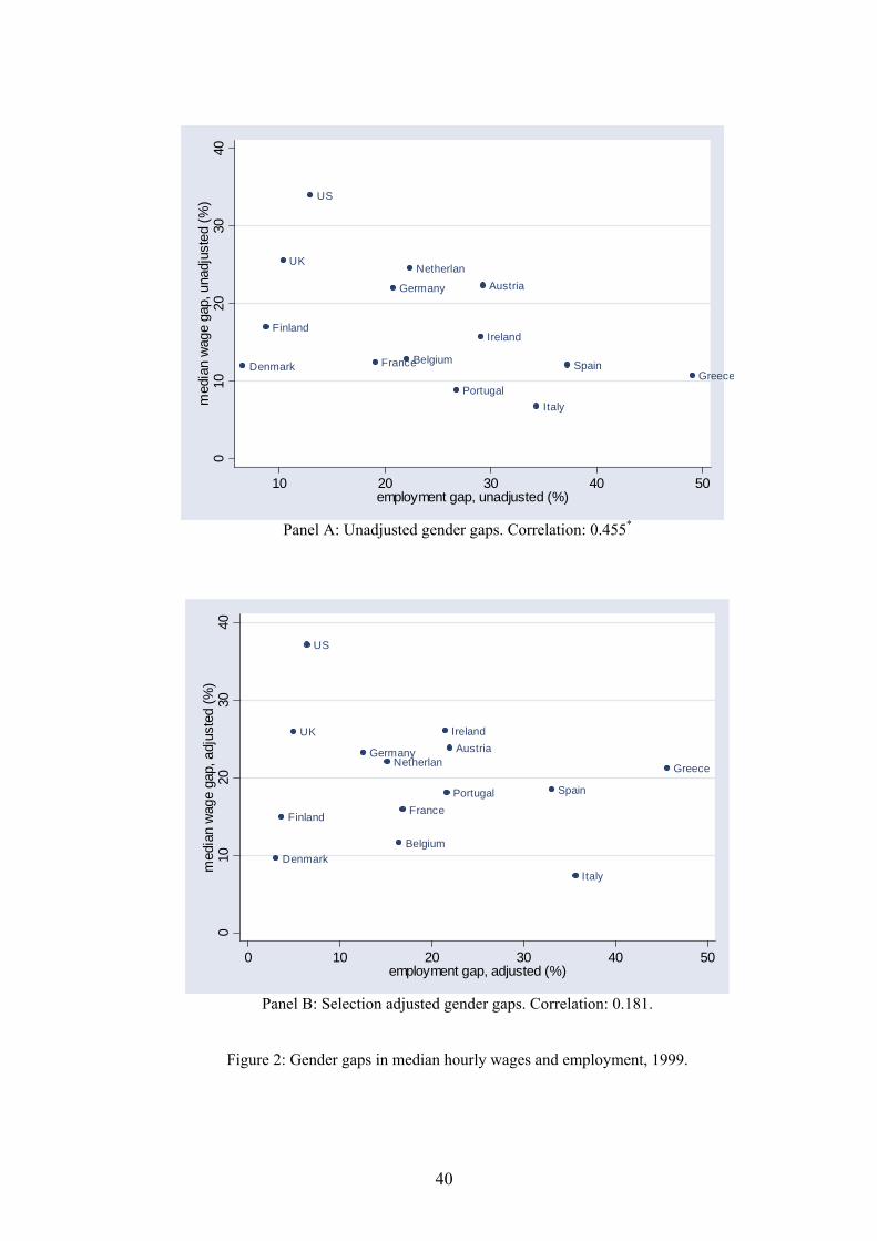
The relationship between wage and employment gaps is represented in Figure 1. The coefficient of

correlation between them is -0.497 and is significant at the 7% level.

Such negative correlation between wage and employment gaps may reveal significant sample

selection effects in observed wage distributions. If the probability of an individual being at work

is positively affected by the level of her potential wage offers, and this mechanism is stronger for

women than for men, then high gender employment gaps become consistent with relatively low

gender wage gaps simply because low wage women are relatively less likely than men to feature in

observed wage distributions.

Table 1 also reports wage and employment gaps across three schooling levels. Employment

gaps everywhere decline with educational levels, if anything more strongly in southern Europe

than elsewhere. On the other hand, the relationship between gender wage gaps and education

varies across countries. While the wage gap is either flat or rises slightly with education in most

countries, it falls sharply with education in Ireland and southern Europe. In particular, if one

looks at the low-education group, the wage gap in southern Europe is closely comparable to that of

other countries - while being much lower for the high-education group. However, the fact that the

low-education group has the lowest weight in employment makes the overall wage gap substantially

lower in southern Europe.

Interestingly, in southern Europe countries, the overall wage gap tends to be smaller than each

of the education-specific gaps, and thus lower than their weighted average. One can think of this

difference in terms of an omitted variable bias. The overall gap is simply the coefficient on the

male dummy in a wage equation that only controls for gender. The weighted average of the three

education-specific gaps would be the coefficient on the male dummy in a wage equation that controls

for both gender and education. Education would thus be an omitted variable in the first regression,

7Similarly as in other Scandinavian countries, the employment gap in Sweden over the same sample period is 5.2percentage points.

10

and the induced bias has the sign of the correlation between education and the male dummy, given

that the correlation between education and the error term is positive. While the overall correlation

between education and the male dummy tends to be positive in all countries, such correlation

becomes negative and fairly strong among the employed in southern Europe, lowering the overall

wage gap below each of the education-specific wage gaps. The fact that, conditional on being

employed, southern European women tend to be more educated than men may be itself interpreted

as a signal of selection into employment based on high-wage characteristics.

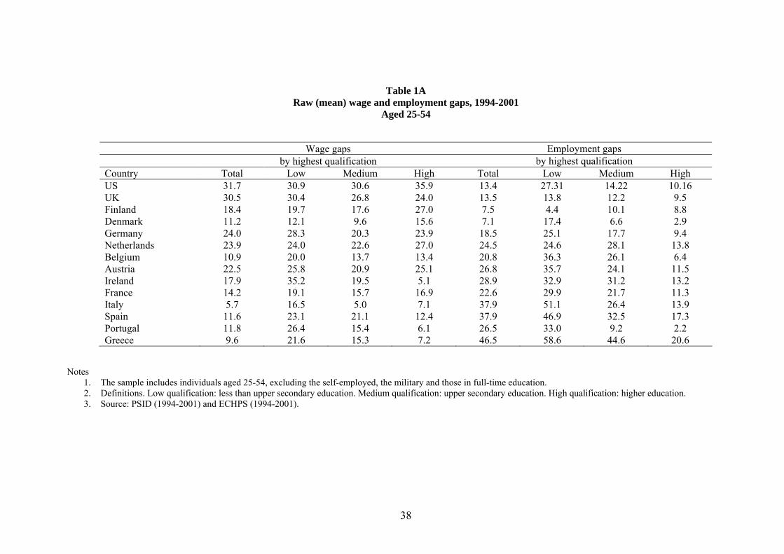
In Table 1A we report similar gaps for the population aged 25-54, as international differences in

schooling and/or retirement systems may have affected relevant gaps for the 16-64 sample. However,

when comparing the figures of Table 1 and 2, we do not find evidence of important discrepancies

between the gender gaps computed for those aged 16-64 and those aged 25-54. The rest of our

analysis therefore uses the population sample aged 16-64.

4 Methodology

We are interested in measuring the gender wage gap:

D = E (w|X,male)−E (w|X, female) , (1)

where D denotes the gender gap in mean log wages, w denotes log wages and X is a vector of

observable characteristics. Average wages for each gender are given by:

E (w|X, g) = E (w|X, g, I = 1)Pr(I = 1|X, g) +E (w|X, g, I = 0) [1− Pr(I = 1|X, g)], (2)

where I is an indicator function that equals 1 if an individual is employed and zero otherwise

and g =male, female. Wage gaps estimated on observed wage distributions are based on the

E (w|X, g, I = 1) term alone. If there are systematic differences between E (w|X, g, I = 1) and

E (w|X, g, I = 0), cross-country variation in Pr(I = 1|X, g)may translate into misleading inferences

concerning the international variation in potential wage offers. This problem typically affects esti-

mates of female wage equations; even more so when one is interested in cross-country comparisons

of gender wage gaps, given the cross-country variation in Pr(I = 1|X,male)− Pr(I = 1|X,female),

measuring the gender employment gap. Our goal is to retrieve gender gaps in potential (offer)

wages, as illustrated in (1), where E (w|X, g) is given by (2). For this purpose, the data provide

information on both E (w|X, g, I = 1) and Pr(I = 1|X, g), but clearly not on E (w|X, g, I = 0) , as

wages are only observed for those who are in work.

11

A number of approaches can be used to correct for non-random sample selection in wage equa-

tions and/or recover the distribution in potential wages. The seminal approach suggested by Heck-

man (1974, 1979) consists in allowing for selection on unobservables, i.e. on variables that do not

feature in the wage equation but that are observed in the data.8 Heckman’s two-stage parametric

specifications have been used extensively in the literature in order to correct for selectivity bias in

female wage equations. More recently, these have been criticized for lack of robustness and distrib-

utional assumptions (see Manski, 1989). Approaches that circumvent most of the criticism include

semi-parametric selection correction models that appeared in the literature since the early 1980s

(see Vella, 1998, for an extensive survey of both parametric and non-parametric sample selection

models). Two-stage nonparametric methods allow in principle to approximate the bias term by a

series expansion of propensity scores from the selection equation, with the qualification that the

term of order zero in the polynomial is not separately identified from the constant term in the

wage equation, unless some additional information is available (see Buchinski, 1998). Usually, the

constant term in the wage regression is identified from a subset of workers for which the probability

of work is close to one, but in our case this route is not feasible since for no type of women the

probability of working is close to one in all countries.

Selection on observed characteristics is instead exploited in the matching approach, which con-

sists in imputing wages for the non-employed by assigning them the observed wages of the employed

with matching characteristics (see Blau and Beller, 1992, and Juhn, 1992, 2003).

The approach of this paper is also based on some form of wage imputation for the non-employed,

but it simply requires assumptions on the position of the imputed wage observations with respect

to the median of the wage distribution, and not on their level, as in Johnson et al. (2000) and

Neal (2004).9 We then estimate median wage gaps on the resulting imputed wage distributions,

i.e. on the enlarged wage distribution that is obtained implementing alternative wage imputation

methods for the nonemployed. The attractive feature of median regressions is that, if missing

wage observations fall completely on one or the other side of the median regression line, the results

are only affected by the position of wage observations with respect to the median, and not by

specific values of imputed wages, as it would be in the matching approach. One can therefore make

8 In this framework, wages of employed and nonemployed would be recovered as

E (w|X, g, I = 1) = Xβ +E (ε1|ε0 > −V γ)E (w|X, g, I = 0) = Xβ +E (ε1|ε0 < −V γ) ,

respectively, where V is the set of covariates used in the selection equation, with associated parameters γ, and ε1 andε0 are the error terms in the wage and the selection equation, respectively.

9See also Chandra (2003) for a non-parametric application to racial wage gaps among US men.

12

assumptions motivated by economic theory on whether an individual who is not in work should have

a wage observation below or above median wages, conditional on characteristics. When estimating

raw gender wage gaps, the only characteristic included is a gender dummy. Thus one should simply

make assumptions on whether a nonemployed individual should earn above- or below-median wages

for their gender.

More formally, let’s consider the linear wage equation

wi = Xiβ + εi, (3)

where wi denotes (log) wage offers, Xi denotes characteristics, now also including gender, with

associated coefficients β, and εi is an error term such that Med (εi|Xi) = 0. Let’s denote by β the

hypothetical LAD estimator based on true wage offers. However, wage offers wi are only observed

for the employed, and missing for non-employed. Suppose that missing wage offers fall completely

below the median regression line, i.e. wi < Xibβ for the non-employed (Ii = 0). Then one can then

define a transformed dependent variable yi that is equal to wi for Ii = 1 and to some arbitrarily

low imputed value ewi for Ii = 0, and the following result holds:

βimputed ≡ argminβ

NXi=1

|yi −X0iβ| = β ≡ argmin

β

NXi=1

|wi −X0iβ|. (4)

Condition (4) states that the LAD estimator is not affected by imputation (see Bloomfield and

Steiger, 1983, pp. 44-52, for details). Clearly, (4) also holds when missing wage offers fall completely

above the median regression line, i.e. wi > Xibβ, and yi is set equal to some arbitrarily high

imputed value ewi for the non-employed. More in general, the LAD estimator is also not affected by

imputation when missing wage offers fall on both sides of the median, provided that observations

on either side are imputed correctly, and that the median does not fall within either of the imputed

sets. For example, suppose that the potential wages of the non-employed could be classified in two

groups, A and B, such that wi > Xibβ for i ∈ A and wi < Xi

bβ for i ∈ B, i.e. the predicted median

does not belong to either A or B. If yi is set equal to some arbitrarily high value for all i ∈ A and

equal to some arbitrarily low value for all i ∈ B, LAD inference is still valid.

It should be noted, however, that in order to use median regressions to evaluate gender wage

gaps in (1) one should assume that the mean and the median of the (log) wage distribution coincide,

in other words that the (log) wage distribution is symmetric. This is clearly true for the log-normal

distribution, which is typically assumed in Mincerian wage equations. In what follows we therefore

13

assume that the distribution of offer wages is log-normal.10

Having said this, imputation can be performed in several ways, which we describe below.

Imputation on unobservables. We first exploit the panel nature of our data sets and, for all

those not in work in some base year, we recover hourly wage observations from the nearest wave in

the sample. The underlying identifying assumption is that an individual’s position with respect to

the base-year median, conditional on X, can be recovered looking at the level of her wage in the

nearest wave. As the position with respect to the median is determined using levels of wages in

other waves in the sample, we are allowing for selection on unobservables.

This procedure of imputation makes sense when an individual’s position in the latent wage

distribution stays on the same side of the median when switching employment status. As we

estimate median wage gaps, we do not need an assumption of stable rank throughout the whole wage

distribution, but only with respect to the median. It may be interesting to interpret our identifying

assumption in the context of the framework developed by Di Nardo, Fortin and Lemieux (1996) in

order to estimate counterfactual densities of wages. In doing this, they assume that the structure

of wages, conditional on a set of individual characteristics, does not depend on the distribution

of characteristics themselves, i.e. it would be the same both in the actual and the counterfactual

states of the world. If our objective were to recover the counterfactual density of wages that would

be observed if all individuals were in work, we would need to assume that the distribution of wage

offers, conditional on X, were the same whether one is employed or nonemployed. However, as we

aim at recovering just the median of such counterfactual density of wages, conditional on X, we

need a much weaker identifying assumption, namely that the cumulative density of wages up to

the median include the same individuals in the actual and counterfactual states of the world. In

other words, if the position of individuals in the latent wage distribution changes with employment

status, movements that happen within either side of the median do not invalidate this method.

While imputation based on this procedure arguably exploits the minimum set of potentially

arbitrary assumptions, it has the disadvantage of not providing any wage information on individuals

who never worked during the sample period. It is therefore important to understand in which

direction this problem may distort, if at all, the resulting median wage gaps. If women are on

10 If one does not impose symmetry of the (log) wage distribution, the equivalent of (2) would be

Med (w|X, g) = F−1(1/2)

= F−1 {F [Med (w|X, g, I = 1)]Pr(I = 1|X, g) + F [Med (w|X, g, I = 1)] [1− Pr(I = 1|X, g)]} .

14

average less attached to the labor market than men, and if individuals who are less attached have on

average lower wage characteristics than the fully attached, then the difference between the median

gender wage gap on the imputed and the actual wage distribution tends to be higher the higher the

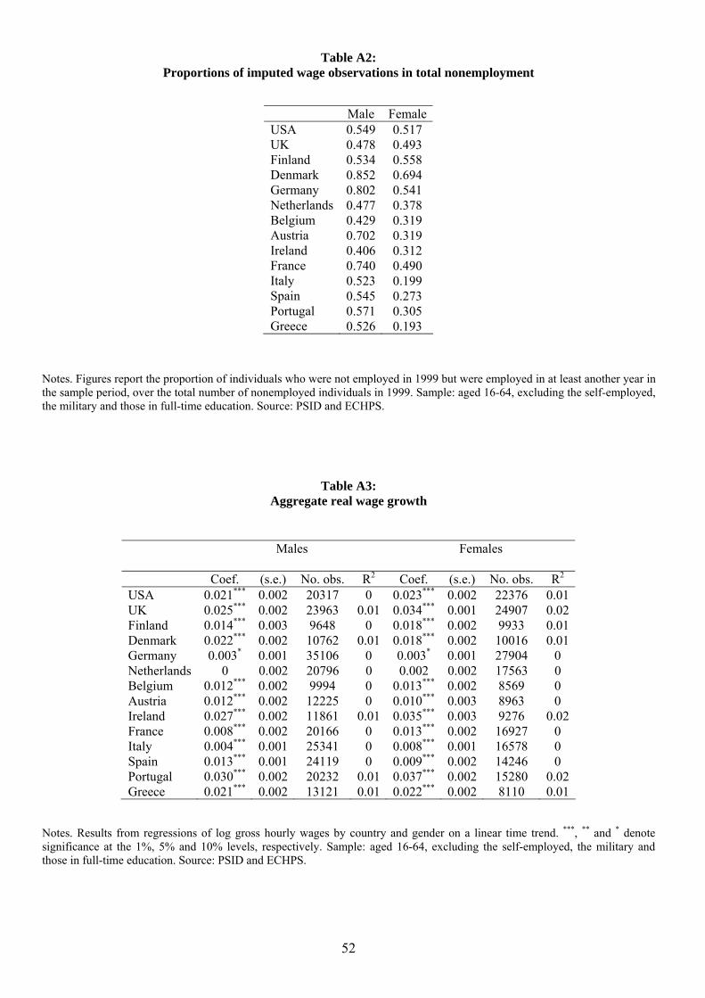
proportion of imputed wage observations in total non-employment in the base year. Consider for

example a country with very persistent employment status: those who do not work in the base year

and are therefore less attached are less likely to work at all in the whole sample period. In this case

low wage observations for the less attached are less likely to be recovered, and the estimated wage

gap is likely to be lower. Proportions of imputed wage observations over the total non-employed

population in 1999 (our base year) are reported in Table A2: the differential between male and

female proportions tends to be higher in Germany, Austria, France and southern Europe than

elsewhere. Under reasonable assumptions we should therefore expect the difference between the

median wage gap on the imputed and the actual wage distribution to be biased downward relatively

more in this set of countries. This in turn means that we are being relatively more conservative in

assessing the effect of non-random employment selection in these countries than elsewhere.

Even so, it would of course be preferable to recover wage observations also for those never

observed in work during the whole sample period. To do this, we rely on the observed characteristics

of the nonemployed.

Imputation on observables. We perform imputation based on observable characteristics in

two ways. First, we can recover wage observations for the non-employed by making assumptions

about whether they place above or below the median wage offer, conditional on X, based on a small

number of characteristics. Let’s summarize these characteristics in a vector Z: in our specifications,

Z will include, in turn, employment status (unemployed versus out of the labor force), education

and work experience, and spouse income. Of course Z cannot include any of the variables in the

X-vector (trivially, one cannot use human capital variables to impute missing wage observations in

the estimation of human-capital corrected wage gaps). While this condition is easy to meet when

estimating raw wage gaps, i.e. when the X-vector only contains a gender dummy, it becomes hard

to satisfy when estimating gender gaps adjusted for characteristics. We will come back to this in

Section 6.

This imputation method for placing individuals with respect to the median follows a sort of

educated guess, based on their observable characteristics. However, we again use wage information

from other waves in the panel to assess the goodness of such guess.

We also use probability models for imputation of missing wage observations, based on Rubin’s

15

(1987) two-step methodology for repeated imputation inference.11 In the first step a statistical

model is chosen for wage imputation, which should be closely related to the nature of the missing-

data problem. In the second step one obtains (a small number of) repeated and independent

imputed samples. The final estimate for the statistic of interest is obtained by averaging the

estimates across all rounds of imputation. The associated variances take into account variation

both within and between imputations (see the Appendix for details).

In the first step we use multivariate analysis in order to estimate the probability of an indi-

vidual’s belonging above or below the median of the wage distribution, conditional on X. Assume

for simplicity that X only contains a gender dummy. On the sub-sample of employed workers

we build an indicator function Mi that is equal to one for individuals whose wage is higher than

the median of the observed wage distribution for their gender and zero otherwise. We then esti-

mate for each gender a probit model for Mi, with explanatory variables Zi that are available for

both the employed and the non-employed sub-samples, typically human capital controls. Using the

probit estimates we obtain predicted probabilities of having a latent wage above the median for

each gender, Pi = Φ(bγZi) = Pr(Mi = 1|Zi), for the nonemployed subset, where Φ is the c.d.f. of

the standardized normal distribution and bγ is the estimated vector of parameters from the probit

regression. The predicted probabilities Pi are then used in the second step as sampling weights

for the nonemployed. That is, in each of the independent imputed samples, employed individuals

feature with their observed wage, and nonemployed individuals feature with a wage above median

with probability Pi and a wage below median with probability 1− Pi.

The repeated imputation procedure effectively uses all the information available for individuals

who are not observed in work at the time of survey. We compare this methodology to what may

be defined as simple imputation. That is, having estimated predicted probabilities Pi of belonging

above the median for those not in work, we assign them wages above the median if Pi > 0.5 and

below otherwise. This simple imputation procedure tends to overestimate the median gender wage

gap on the imputed sample if there is a relatively large mass of non-employed women with Pi < 0.5

but very close to 0.5.

As discussed in Rubin (1987), one of the advantages of repeated imputation is that it reflects

uncertainty about the reason for missing information. While simple imputation techniques such as

11See Rubin (1987) for an extended analysis of this technique and Rubin (1996) for a survey of more recentdevelopments. The repeated imputation technique was developed by Rubin as a general solution to the statisticalproblem of missing data in large surveys, being mostly due to non-reponses. Imputations can be created underBayesian rules, and repeated imputation methods can be interpreted as an approximate Bayesian inference for thestatistics of interest, based on observed data. In this paper, we abstract from Bayesian considerations and apply themethodology in our non-Bayesian framework.

16

regression or matching methods assign a value to the missing wage observation in a deterministic

way (given characteristics), repeated imputation is based on a probabilistic model, i.e. on repeated

random draws under our chosen model for non-employment. Hence, unlike simple imputation,

inference based on repeated imputation takes into account the additional variability underlying the

presence of missing values.

Similarly as when making imputation based on wage information from adjacent waves, we need

to assume some form of separability between the structure of wages and individual employment

status. In particular we need to assume that, conditional on our vector of attributes, individuals

stay on the same side of the median whether they are employed or nonemployed.

In both simple and repeated imputation, we initially estimate a probit model for the probability

of belonging above or below the median of the observed wage distribution. However, precisely due

to selection, such median may be quite different from that of the potential wage distribution, i.e.

the median that would be observed if everyone were employed. This could introduce important

biases in our estimates on the imputed sample. In order to attenuate this problem we also perform

repeated and simple imputation on an expanded sample, augmented with wage observations from

adjacent waves. This allows us to get a better estimate of the “true” median in the first step of

our procedure, thus generating more appropriate estimates of the median wage gap on the final,

imputed sample. Note that in this case we are combining imputation on both observables and

unobservables.

It is worthwhile to discuss here the main differences between alternative imputation methods,

also in light of the interpretation of the results presented in the next section. Our imputation

methods differ in terms of the underlying identifying assumptions and of resulting imputed samples.

The first method, where missing wages are imputed using wage information from adjacent waves,

implicitly assumes that an individual’s position with respect to the median can be proxied by their

wage in the nearest wave in the panel. With this procedure one can recover at best individuals who

worked at least once during the eight-year sample period. We thus want to emphasize that this

is a fairly conservative imputation procedure, in which we impute wages for individuals who are

relatively weakly attached to the labor market, but not for those who are completely unattached

and thus never observed in work. While this may affect our estimates (and we will discuss how

in the next section), this procedure has the advantage of restricting imputation to a relatively

“realistic” set of potential workers.

In the second and third imputation methods, we assume instead that an individual’s position

17

with respect to the median can be proxied by a small number of observable characteristics. In

the second method, we take educated guesses regarding the position in the wage distribution of

someone with given characteristics. This procedure is more accurate the more conservative the

criteria used for imputation. For example, assigning individuals with college education above the

median and individuals with no qualifications below the median is more conservative and probably

more accurate than assigning all those with higher than average years of schooling above the

median and all the rest below the median. With this method, our imputed sample is typically

larger than the one obtained with the first method, although still substantially smaller than the

existing population. Finally, with the third method, we estimate the probability of belonging

above the median for the whole range of our vector of characteristics, thus recovering predicted

probabilities and imputed wages for the whole existing population - except of course those with

missing information on characteristics.

Different imputed samples will have an impact on our estimated median wage gaps. In so far

women are more likely to be non-employed than men, and non-employed individuals are more likely

to receive lower wage offers than employed ones, the larger the imputed sample with respect to the

actual sample of employed workers, the larger the estimated correction for selection.

Having said this, it is important to stress that with all three imputation methods used there is

nothing that would tell a priori which way correction for selection is going to affect the results. This

is ultimately determined by the wages that the nonemployed earned when they were previously (or

later) employed, and by their observable characteristics, depending on methods.

With these clarifications in mind, we move next to the description of our results.

5 Results on raw wage gaps

5.1 Imputation based on unobservables

Our first set of results refers to imputation based on unobservable characteristics. This means

that an individual’s position with respect to the median of the wage distribution is proxied by the

position of their wage obtained from the nearest available wave.

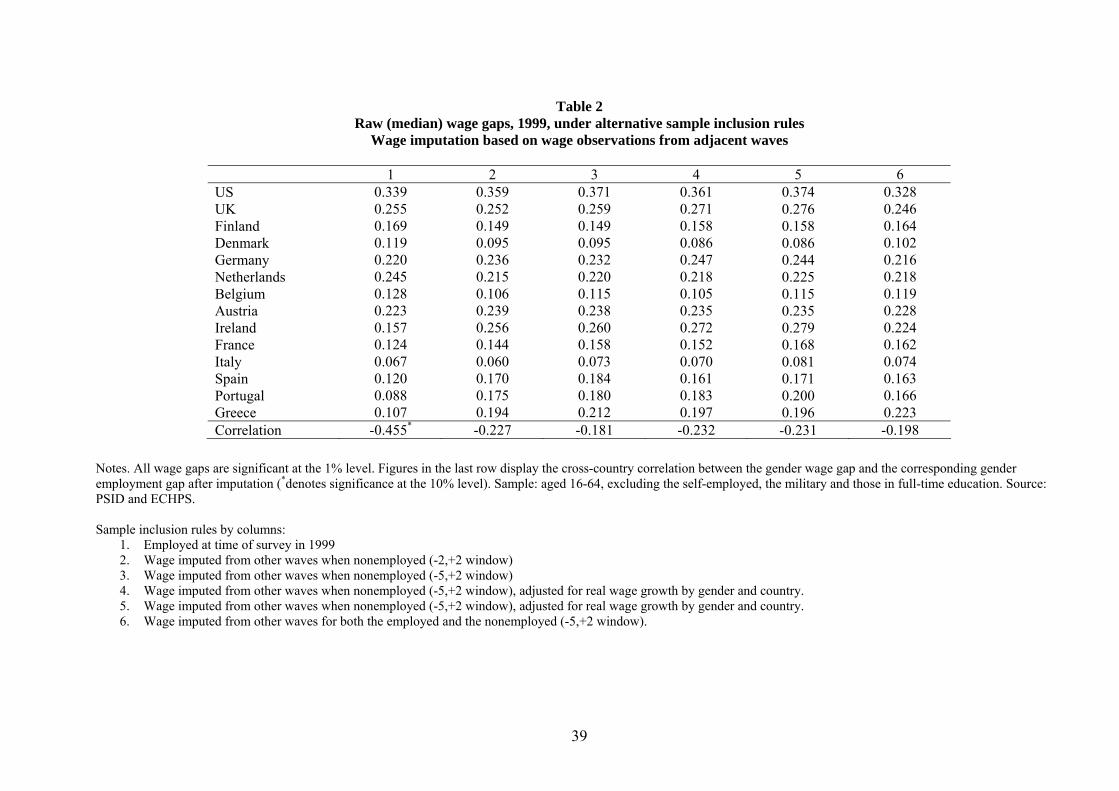
The results are reported in Table 2. Column 1 reports raw (unadjusted) wage gaps for individ-

uals with hourly wage observations in 1999, which is our base year. These replicate very closely the

wage gaps reported in Table 1, with the only difference that mean wage gaps for the whole sample

period are reported in Table 1, while median wage gaps for 1999 are reported here. As in Table 1,

the US and the UK stand out as the countries with the highest wage gaps, followed by central and

18

northern Europe, and finally Scandinavia and Southern Europe.

In column 2 missing wage observations in 1999 are replaced with the real value of the nearest

wage observation in a 2-year window, while in column 3 they are replaced with the real value

of the nearest wage observation in the whole sample period, meaning a maximum window of [-

5, +2] years. Comparing figures in columns 1-3, one can see that the median wage gap remains

substantially unaffected or affected very little in the US, the UK, and a number of European

countries down to Austria, and increases substantially in Ireland, France and southern Europe, this

latter group including countries with the highest gender employment gap. While sample selection

seems to be fairly neutral in a large number of countries in our sample, or, in other words, selection

in market work does not seem to vary systematically with wage characteristics of individuals, it is

mostly high-wage individuals who work in Ireland, France and southern Europe, and this seems bias

downward the estimate of the gender wage gap when one does not account for non-random sample

selection. Note finally that in Scandinavian countries and the Netherlands the wage gap in potential

wages decreases slightly, if anything providing evidence of an underlying selection mechanism of

the opposite sign.

Arulampalan, Booth and Bryan (2007) find evidence of glass ceilings, defined as a difference of

at least 2 points between the 90th percentile (adjusted) wage gap and the 75th or the 50th per-

centile gap, in most European countries, and evidence of sticky floors, defined as a difference of at

least 2 points between the 10th percentile (adjusted) wage gap and the 25th or 50th percentile gap,

only in Germany, France, Italy and Spain (but report no evidence for Portugal or Greece). Sticky

floors for low-educated women in Spain are also documented by De La Rica, Dolado and Llorens

(2007). Similarly, our descriptive evidence of section 3.3 shows a strongly decreasing wage gap in

levels of education in southern Europe. High wage gaps at the bottom of the wage distribution in

some southern European countries may discourage employment participation of low-wage women

relatively more than in other countries. This would be consistent with a sizeable impact of employ-

ment selection at the bottom of the wage distribution in these countries. Our selection-corrected

estimates for the gender wage gap precisely go in this direction.

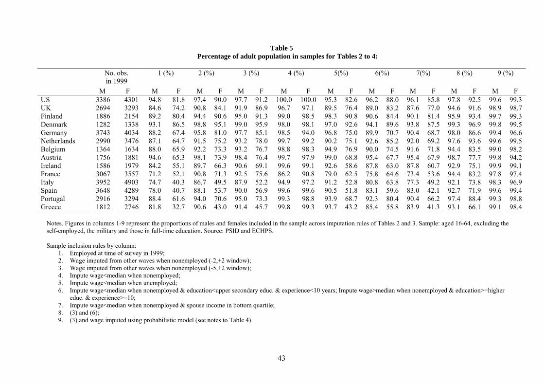
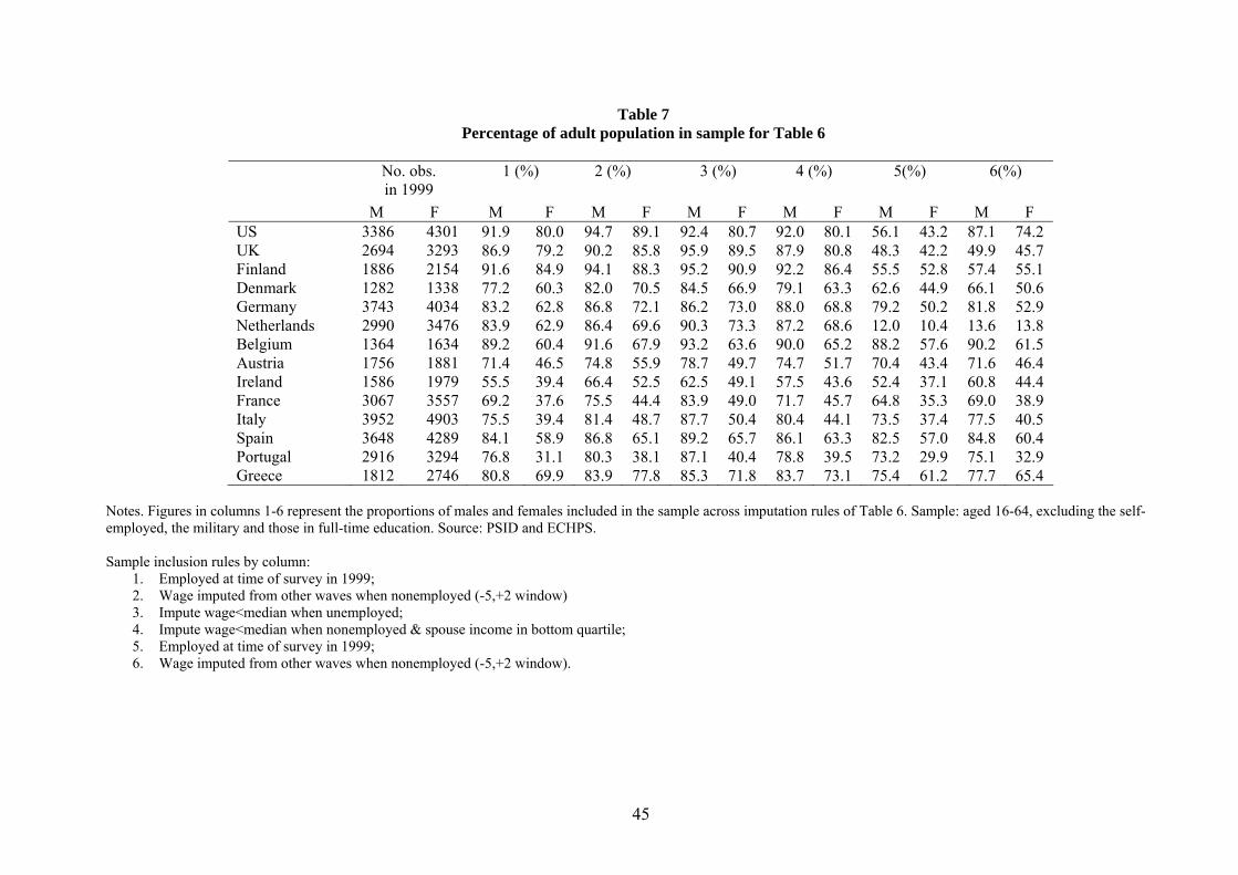
For each sample inclusion rule in column 1-3 one can compute the adjusted employment rate for

each gender, i.e. the proportion of the adult population that is either working or has an imputed

wage. These proportions are reported in columns 1-3 of Table 5. When moving from column 1 to 3,

the fraction of women included increases substantially in southern Europe, and only slightly less in

countries like Germany or the UK, where the estimated wage sample is not greatly affected by the

sample inclusion rules. Moreover, the fraction of men included in the sample also increases across

19

imputation rules. It is thus not simply the lower female employment rate in several countries that

determines our findings, it is also the fact that in some countries selection into work seems to be

less correlated to wage characteristics than in others.

As one would expect from our cross-country results, controlling for selection removes most of the

observed negative correlation between wage and employment gaps. At the bottom of each column

in Table 2 we compute the coefficient of correlation between the wage gap in the same column and

the adjusted employment gap, as obtained from the relevant column of Table 5. The correlation

coefficient between unadjusted median wage gaps and employment gaps is -0.455, and is significantly

different from zero at the 10% level. Using the adjusted estimates from column 3, this falls to -0.181,

and is not significantly different from zero at standard levels. The importance of sample selection

can also be grasped graphically by looking at Figure 2, which shows the relationship between

median wage and employment gaps, either unadjusted (estimates from column 1) or selection-

adjusted (estimates from column 3). While a downward-sloping pattern can be detected in Panel

A, Panel B rather shows a random scatter-plot.

The estimates of columns 2 and 3 do not control for aggregate wage growth over time. If

aggregate wage growth was homogeneous across genders and countries, then estimated wage gaps

based on wage observations for other waves in the panel would not be not affected. But if there

is a gender differential in wage growth, and if such differential varies across countries, then simply

using earlier (later) wage observations would deliver a higher (lower) median wage gap in countries

where women have relatively lower wage growth with respect to men.12 We thus estimate real wage

growth by regressing log real hourly wages for each country and gender on a linear trend.13 The

resulting coefficients are reported in Table A3. These are then used to adjust real wage observations

outside the base year and re-estimate median wage gaps. The resulting median wage gaps on the

imputed wage distribution are reported in column 4 and 5. Despite some differences in real wage

growth rates across genders and countries, adjusting estimated median wage gaps does not produce

any appreciable change in the results reported in columns 2 and 3, which do not control for real

wage growth.

As explained in Section 4, imputation based on wages from adjacent waves relies on the iden-

tifying assumption that individuals stay on the same side of their gender median across different

12Note however that, even if real wage growth were homogeneous across genders, imputation based on wageobservations from adjacent waves would not be affected only if the proportion of men and women in the sampleremained unchanged after imputation.13Of course, for our estimated rates of wage growth to be unbiased, this procedure requires that participation into

employment be unaffected by wage growth, which may not be the case.

20

waves in the panel. Some indirect evidence on the validity of such assumption can be gathered by

ignoring all available wage observations for 1999, and proceeding to impute them as we did for the

missing wage observations. If our identifying assumption is largely correct, the results obtained

on the “all”-imputed wage distribution should closely mimic those obtained by imputing missing

wages only. Column 6 in Table 2 reports such estimates, using imputed wages from all existing

waves. The resulting series of estimated wage gaps is very similar to that reported in column 3,

and so is the correlation with the corresponding employment gaps.

Note that in Table 2 we are (at best) recovering on average 24% of the non-employed females

in the four southern European countries, as opposed to approximately 46% in the rest of countries

(see Table A2). For men, the respective proportions are 54% and 60%. Such differences happen

because (non)employment status tends to be more persistent in southern Europe than elsewhere,

and much more so for women than for men. As briefly noted in Section 3, given that we recover

relatively fewer less-attached women in southern Europe, we are being relatively more conservative

in assessing the effect of non-random employment selection in southern Europe than elsewhere.

For this reason it is important to try to recover wage observations also for those never observed

in work in any wave of the sample period, as explained in the next section.

5.2 Imputation based on observables

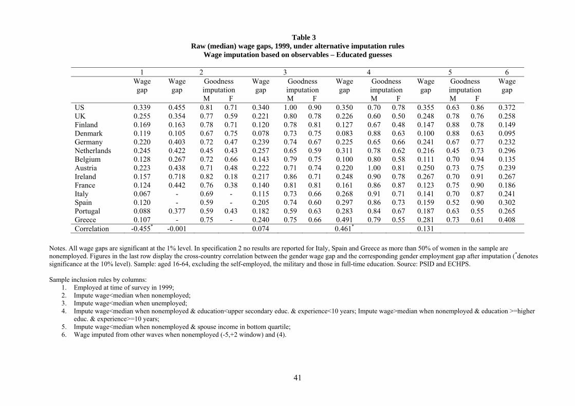
In Table 3 we estimate median wage gaps on imputed wage distributions, making assumptions on

whether individuals who were nonemployed in 1999 had potential wage offers above or below the

median for their gender. Column 1 reports for reference the median wage gap on the base sample,

which is the same as the one reported in column 1 of Table 2. In column 2 we assume that all

those not in work would have wage offers below the median for their gender.14 This is an extreme

assumption, and should only be taken as a benchmark. This assumption is clearly violated in cases

like Italy, Spain and Greece, in which more than a half of the female sample is not in work in

1999, as by definition all missing observations cannot fall below the median. For this reason we

do not report estimated gaps for these three countries. However, also for other countries there are

reasons to believe that not all nonemployed individuals would have wage offers below their gender

mean. Of course, we cannot know exactly what wages these individuals would have received if they

had worked in 1999. But we can form an idea of the goodness of this assumption looking again

at wage observations (if any) for these individuals in all other waves of the panel. This allows us

14 In the practice, whenever we assign someone a wage below the median we pick wi = −5, this value being lowerthan the minimum observed (log) wage for all countries, and thus lower than the median. Similarly, whenever weassign someone a wage above the median we pick wi = 20.

21

to compute what proportion of imputed observations had at some point in time wages that were

indeed below their gender median. Such proportions are also presented separately for each gender

in column 2. They are fairly high for men, but sensibly lower for women, which makes the estimates

based on this extreme imputation case a benchmark rather than a plausible measure for the gender

wage gap. Having said this, estimated median wage gaps increase substantially for most countries,

except Denmark and Finland.

We next make imputations based on observed characteristics of nonemployed individuals. In

column 3 we impute a wage below the median to all those who are unemployed (as opposed to

non participants) in 1999. The unemployed by definition are receiving wage offers (if any) below

their reservation wage, as it follows from search theory, while the employed have received at least

one wage offer above their reservation wage. At constant reservation wages, the unemployed have

lower potential wages than the observed wages of the employed, and are thus assigned a fictitious

wage value below the median. This imputation leaves the median wage gap roughly unchanged

with respect to the base sample everywhere down to Austria, and raises it substantially in Ireland,

France and southern Europe. Also, the proportion of “correctly” imputed observations, computed

as for the previous imputation case, is now much higher. Those who do not work because they

are unemployed are thus relatively more likely to be over-represented in the lower half of the wage

distribution.

In column 4 we follow standard human capital theory and assume that all those with less than

upper secondary education and less than 10 years of potential labor market experience have wage

observations below the median for their gender. Those with at least higher education and at least

10 years of labor market experience are instead placed above the median. In the four southern

European countries the gender wage gap increases substantially: with respect to the imputation

rule of column 3, it doubles in Italy and Greece and it increases by 10 log points in Spain and

Portugal. This finding underscores the importance of selection with respect to human capital in

southern Europe. For this set of countries, except Greece, the proportions of correctly imputed

observations for men and women also generally increases relative to column 3. Interestingly, this

is not the case for the US, the UK, Finland, Denmark and Germany, where imputation based on

unemployment works better than imputation based on human capital components.

The imputation method of column 5 is implicitly based on the assumption of assortative mating

along wage attributes and consists in assigning wages below the median to those whose partner

has total income in the bottom quartile of the gender-specific distribution. The results are broadly

similar to those of column 3: the wage gap is mostly affected in Ireland and southern Europe. It

22

would be natural to perform a similar exercise at the top of the distribution, by assigning a wage

above the median to those whose partner has total income in the top quartile. However, in this

case the proportion of correctly imputed observations was too low to rely on the assumption used

for imputation.

We also make imputation based on observable characteristics to recover wage observations

only for those who never worked, using first wage observations available from other waves, and

then imputing the remaining missing ones using education and experience information as done in

column 4. The results, reported in column 6, show again a much higher gender gap in Ireland,

France, and southern Europe, and not much of a change elsewhere with respect to the base sample

of column 1.

Similarly as with the previous imputation method, we report in columns 4-8 of Table 5 the

proportion of men and women included in our imputed samples. As expected, we are now able to

recover wage information for a higher fraction of the adult population.15 The correlations between

median wage gaps on the imputed wage distribution and the corresponding adjusted employment

gaps, reported in the bottom row of Table 3, are once again not significantly different from zero at

standard significance levels. The notable exception is column 4, where the correlation between the

two series becomes positive, large, and statistically significant. This is due to the fact that, under

this imputation rule, the estimated gender wage gap in southern Europe increases disproportion-

ately relative to other countries, while the employment gap on the imputed sample is much less

affected.16

We finally use a probabilistic model for assigning individuals wages above or below their gender

median, using both simple and repeated imputation techniques. As mentioned above, this involves

a two-step procedure, using once more data for 1999 as our base year. In the first step we estimate a

probit model for the probability that an individual with a non-missing wage falls above their gender

median, given a set of characteristics. We estimate both a simple human capital specification that

controls for education (two dummies for upper secondary and higher education), experience and

its square; and a more general specification that also controls for marital status, the number of

children of different ages (between 0 and 2, 3 and 5, 6 and 10, and 11 and 15 years old), and

the position of the spouse in their gender specific distribution of total income (three dummies

15 In column 4 such proportions are generally not equal to 100% because we did not impute wages to those whoare employed but have missing information on hourly wages due to non-response, as the selection mechanism drivingnon-response is clearly different from that driving nonemployment.16We have also computed the correlations between median wage gaps from the imputed wage distribution and

employment gaps from the base sample. For all imputation rules, the resulting correlation coefficients were positiveand statistically significant. In our tables we are thus reporting the more conservative values.

23

corresponding to the three highest quartiles). Since the results of the exercise do not vary in any

meaningful way across specifications, we only report findings for the human capital specification.

The estimated coefficients for the first-stage probit regression (not reported) conform to standard

economic theory: individuals with higher levels of educational attainment and/or of labor market

experience are more likely to feature in the top half of the wage distribution.

In the second step we use the probit estimates to compute the predicted probability that a

missing wage observation falls above the gender median. We use two alternative methods to impute

wages within this framework. With the first method, which we define simple imputation, we impute

a value of the wage above (below) the median if the predicted probability is greater (smaller) than

0.5. This implies that a missing-wage observation is assigned a value below median even if it would

only marginally feature in the bottom part of the wage distribution. Our second method is based

on the repeated imputation methodology discussed in Section 4. We construct 20 independent

imputed samples. In each imputed sample, the employed feature with their observed wage, while

for each nonemployed we “draw” her position with respect to the median using her predicted

probability from the probit model. Specifically, we draw independent random numbers from a

uniform distribution with support [0,1] and assign a nonemployed worker a wage above (below)

the median if the random draw is lower (higher) than their predicted probability. For each of the

20 samples we estimate the median gender wage gap and obtain the corresponding bootstrapped

standard error.17 For each country and specification, the estimated median wage gap is then

obtained by averaging the estimates across the 20 rounds of imputation. The standard errors are

adjusted to take into account both between and within-imputation variation.

The results for this exercise are summarized in Table 4. Column 1 reports the median wage gap

for the base sample, which is the same as the one reported in column 1 of Table 3. Column 2 reports

the estimated median wage gap using simple imputation. In Column 3 we use simple imputation

to recover wage observations only for those who never worked in the sample period. That is, we

first use wage observations available from other waves to impute missing wages and then impute

the remaining missing ones as done in Column 2. Note that this procedure changes the reference

median wage: by expanding the wage sample we are in practice able to compute a median wage

that is closer to the latent median, i.e. the median that one would observe if everybody were in

work. Columns 4 and 5 report results based on repeated imputation, having computed the reference

median as in columns 2 and 3, respectively.

For all countries, and in particular for Ireland, France and Southern Europe, wage imputation

17We use the STATA command bsqreg where we set the number of replications to 200.

24

generates larger estimates of the median gender wage gap than in the base sample of column 1. The

estimates are of the same order of magnitude than the ones obtained when we assign a wage below

median to all missing wage observations or to all the unemployed individuals with missing wages

(see columns 2 and 3 in Table 3). When we use simple imputation for the base sample (column 2)

we cannot report estimated gaps for Italy, Spain and Greece, as in these countries more than half

of the female sample would be assigned a wage below median, similarly to what we had in column

2 of Table 3.

We first compare the median wage gap obtained with simple imputation on the base sample

(column 2) with that obtained with simple imputation on the sample expanded with wage obser-

vations from other waves (column 3). In the latter case it is now possible to obtain estimated gaps

for Italy, Spain and Greece. This is due to the difference between the reference median wage in the

two columns, and highlights the importance of estimating the median wage on a distribution that

is as close as possible to the latent one. For all countries except the UK and Austria the estimated

median wage gap in column 3 is lower than in column 2. This decline is largest for Belgium, France,

and Southern Europe. The use of the expanded sample seems to allow us to get a better estimate

of the “true” median in the first step of our procedure, thus generating more appropriate estimates

of the median wage gap on the final, imputed sample. The same discussion applies to the results

obtained using repeated imputation (comparing entries in column 4 and column 5).

Second, we compare the results obtained with simple and repeated imputation. Repeated

imputation generates a lower estimate of the median gender gap than simple imputation for almost

all countries. However, this tendency is stronger for Ireland, France and Southern Europe (see

columns 2 and 4). Simple imputation tends to overestimate the gender wage gap when there is a

relatively heavy mass of women with a predicted probability of featuring below the median that is

slightly lower than 0.5, and this turns out to be the case for countries with high gender employment

gaps. Moreover, with repeated imputation we can obtain estimates of the wage gap for Italy and

Spain, since we now assign less than 50% of the female sample below the median. This is still not

the case for Greece.

Repeated imputation on the expanded sample should provide the most accurate estimate of the

median wage gap across countries. Comparing column 1 and column 5 we find that the median wage

gap on the imputed wage distribution increases slightly for the US and the UK, decreases slightly

in Scandinavia and the Netherlands, and stays roughly unchanged in most other central European

countries. However, estimated gender wage gaps on imputed distributions more than double in

Ireland, France and southern Europe. Specifically, the median wage gap in Spain, Portugal and

25

Italy is well above 20 log points, and reaches levels that are comparable to those observed for the

US and the UK both in the base and in the imputed samples. For Greece, we obtain an even larger

estimated gender wage gap (0.5). All the figures in this column are very close to those reported in

column 4 of Table 3. This is not surprising, as the vector of Z variables used for making imputation

is roughly the same, and the only difference between the two sets of results consists in the type of

imputation method (educated guesses in Table 3 versus a statistical model for imputation in Table

4).

Cross-country correlations between wage and employment gaps are reported in the bottom row

of Table 4. The underlying employment rates are now very close to 1 (see column 9 in Table 5),

as the only observations that remain out of the sample are the employed with genuinely missing

wages or those with missing information on human capital characteristics. While the correlation

on the base sample is negative and significant, it becomes not significantly different from zero in

all samples obtained under simple and repeated imputation.

To broadly summarize our findings, one could note that whether one corrects for selection on

unobservables (Table 2) or on observables (Table 3 and 4), our results are qualitatively consistent in

identifying a clear role of sample selection in Ireland, France and southern Europe.18 Quantitatively,

the correction for sample selection is smallest when wage imputation is performed using wage

observation from other waves in the panel, and increases when it is instead performed using observed

characteristics of the nonemployed. As argued above, this is mainly due to different sizes of the

imputed samples. While only individuals with some degree of labor market attachment feature in

the imputed wage distribution in the first case, the use of observed characteristics may in principle

allow wage imputation for the whole population, thus including individuals with no labor market

attachment at all.

The fact that controlling for unobservables does not greatly change the picture obtained when

controlling for a small number of observables alone (education, experience and spouse income)

implies that most of the selection role can indeed be captured by a set of observable individual18We have performed a number of robustness tests and more disaggregate analyses on the results reported in Tables

2 to 4. First, we have restricted the estimates to individuals aged 25-54 in 1999. The results were very similar tothose obtained on the larger sample. Second, for the imputation rules reported in Table 2 and 3, we have repeated ourestimates separately for three education groups (less than upper secondary education, upper secondary education,and higher education), and we found that most of the selection occurs between rather than within groups, as medianwage gaps disaggregated by education are much less affected by sample inclusion rules than in the aggregate. Finally,we have repeated our estimates separately for three demographic groups: single individuals without kids in thehousehold, married or cohabiting without kids, and married or cohabiting with kids. We found evidence of a strongselection effect in Ireland, France and southern Europe among those who are married or cohabiting, especially whenthey have kids, and much less evidence of selection among single individuals without kids.

26

characteristics, and possibly some unobservables closely correlated to them.

6 Results on adjusted wage gaps

Our discussion so far referred to raw wage gaps. In other words, our X vector only contained

a gender dummy in all estimated specifications. The results obtained were specifically targeted

at explaining the main stylized fact highlighted at the beginning of this paper, namely the cross-

country correlation between raw wage and employment gaps.

In this section we move on to the estimation of gender wage gaps adjusted for observable

characteristics, and we compare the unexplained gender gap in earnings across different imputation

rules. Comparisons of adjusted rather than raw wage gaps across sample inclusion or imputation

rules is a further test of whether selection mostly happens along observed or unobserved worker

characteristics.

While similar imputation methods could in principle be used in estimating raw and adjusted

wage gaps, in practice one needs stronger assumptions in order to establish whether a missing

wage observation should be placed above or below the median, as all our imputation rules are

conditional on the vector of covariates included in the wage equation. For example, imagine that

the X vector contains not only a gender dummy but also human capital variables. When missing

wage observations are imputed using wage information from other waves in the panel, one needs

to assume that an individual’s position in the latent wage distribution stays on the same side of

the median across adjacent waves in the panel, conditional on gender and human capital levels.

When observable characteristics are used for imputation, one should be assuming that someone

with characteristics Z should earn a wage, say, below the median, again conditional on their gender

and human capital levels. Hence, all variables in X should be excluded from the Z-vector, which

of course limits the choice of observable characteristics that can be used for imputation. These

caveats and limitations should be borne in mind when interpreting our estimates of adjusted wage

gaps.

We estimate two main specifications across imputation rules: the first one controls human

capital variables and state or region of residence, and the second one also includes job controls. For

the first case, the median wage gap is estimated on the base sample and three alternative imputed

samples, namely (i) a sample enlarged with (the real value of) wage observations from all other

waves in the panel; (ii) a sample enlarged with wage imputation based on unemployment versus

27

inactivity status and (iii) a sample enlarged with wage imputation based on spouse income.19 For

the second case, one would need job controls for the nonemployed, which restricts our choice of

imputation methods to the inclusion of wage observations (and thus job controls) from all other

waves in the panel.

The results are reported in Table 6, and the proportions of the adult population included in

each sample are reported in Table 7. Column 1 of Table 6 reports the median wage gap on the

base 1999 sample, having controlled for education (1 dummy for secondary education completed

and one for college education), experience and its square, and state or region of residence.20 Only

in eight countries out of fourteen is the wage gap adjusted for characteristics lower than the raw

wage gap of column 1, Table 2, and even in those cases the difference between the two is not very

large, except perhaps in the US and the Netherlands. Beyond these two cases, the raw wage gaps

found in Table 2 seem thus largely unexplained by observable characteristics. In particular, in a

number of countries, and especially in southern Europe, the adjusted wage gap is even larger than

the raw wage gap, meaning that employed women have higher wage characteristics than men, again

consistently with some degree of selection with respect to a few observables.

In column 2 the working sample is expanded using available wage observations from other waves

in the panel. Similarly as in Table 2, estimated wage gaps are not greatly affected in the US and in

all European countries down to Austria. They are indeed affected in Ireland, France and southern

Europe, although the increase in the estimated wage gap implied by imputation is much smaller

than that observed on raw wage gaps of Table 2. In particular, using the estimates of columns

1 and 2 of Table 6, correction for selection raises the median wage gap in Ireland, France and

southern EU by an average 14%. The same calculation on the corresponding columns 1 and 3 of

Table 2 gives an average increase of 60%. The interpretation is that selection indeed seems to take

place along a small number of observable characteristics. Conditional on such characteristics, the

employed and nonemployed population look more similar in terms of potential wage offers. Similar

considerations are valid looking at columns 3 and 4 of Table 6, where wage imputation is based on

unemployment status or spouse income in the bottom quartile, although these results seem to be

less reliable, as the proportion of correctly imputed observations is fairly low in some cases.

The estimates presented in columns 5 and 6 also control for job characteristics like occupation

19We do not report estimates for those employed at least once in a window of [-2,+2] years, as they do not provideadditional information from those based on individuals employed at least once in the sample period, nor we reportestimates corrected for real wage growth, as they do not differ much from those of sample (i).20The simplest human capital specification excluding state or region of residence gave very similar results to those

reported here.

28

and industry. The increase in the median wage gap implied by wage imputation is now tiny, except

for the US.21 In most cases virtually all the difference between the wages of the employed and

potential wage offers of the nonemployed can be explained by differences in human capital and in

the potential jobs that the nonemployed would occupy when employed.22

7 Employment selection and wage dispersion

We close the paper with a simple exercise aimed to give a sense of the relative role of employment

selection in the international variation of gender pay gaps vis-à-vis the main competing view, based

on the international variation in overall wage dispersion.

The observed difference in gender pay gaps between two given countries is driven by both gaps

in observed and unobserved characteristics between men and women (reflecting selection), and

differences in the shape of the wage distribution (reflecting inequality). The distinction between

these two factors can be exemplified by making two assumptions. First, changes in the wage

structure have the same impact on all workers earning the same wage, irrespective of their gender.

Second, the position of a worker in the wage distribution is a function of her own characteristics,

as in the standard human capital-competitive market model (see Fortin and Lemieux, 1998, for

a discussion along these lines). Thus the position of the median female wage in the male wage

distribution is a function of differences in gender-specific factors, i.e. of differences between the

characteristics of the median working woman and the median working men in the two countries,

and this is what we call the effect of employment selection.

Suppose that a given country has a male wage distribution F , and a median gender (log) pay

gap β (unadjusted for characteristics). The median female wage in this country corresponds to

quantile q in the male wage distribution, such that

q = F (w(50)− β) (5)

where w(50) represents the median (log) male wage. Variations in the βs across countries can reflect

differences in the wage structure F and/or differences in gender specific factors q. At given wage

structure F , higher q implies lower β. In other words, at given wage structure, a higher female rank21 It would be large in Belgium, but either estimates are not significantly different from zero, probably due to small

sample size for this country.22Estimate of Table 6 are based on the assumption that the returns to characteristics are the same across genders.

We have also relaxed this assumption by estimating separate wage equations for men and women on the base sampleand on that enlarged with wage observations from other waves in the panel, and then applying the well-known Oaxaca(1973) decomposition of the resulting wage gaps into gender differences in characteristics and gender differences in thereturns to characteristics. The component represented by differences in returns should correspond to the unexplainedgender wage gaps of Table 6. The results obtained on the Oaxaca decomposition are in line with those of Table 6.

29

in the male distribution implies a lower median wage gap. At given q, a mean-preserving spread

in F implies higher β, thus higher inequality raises the implied gender wage gap. In this simple

framework the international variation in q represents therefore the role of gender-specific factors,

while variations in β at constant q give an idea of the role of the wage structure.23

In order to assess the relative importance of gender specific factors for a given wage structure

a simple statistic to look at is the cross-country rank correlation between actual pay gaps and

corresponding values of q. A relatively high value of such correlation would tell that the country

ranking of actual wage gaps is similar to the country ranking of differences in gender specific

factors, and this in turn assigns a relatively high explanatory power to the selection story. We then

look at rank correlations between actual wage gaps and the values of q obtained on imputed wage

distributions. As imputation somehow corrects for selection, we expect such correlations to fall.24

The results of this exercise are reported in Table 8. Column 1 reports for reference the actual

values of β for the usual 1999 base sample. Column 2 reports values of q obtained again on the

actual 1999 wage distribution. For example, the interpretation of the first entry in column 2 is that

the median working woman in the US sits at the 29th percentile of the male wage distribution. The

values reported show that working women tend to rank relatively higher in the male distribution

in Scandinavia and, even more so, in southern Europe. Of course, as we have already seen, in

Scandinavia the gender employment gap is very low, and differences in gender specific factors

among the employed roughly reflect differences in the whole adult population. On the other hand,

the employment gap is much higher in southern Europe, and relatively small differences in gender-

specific factors are the result of non-random employment selection. Therefore, in columns 3 to 5

we report the position of the median woman, not just the median employed woman, in the male

earning distribution.

In column 3 we report the values of q obtained using wage observations from all other available

waves to impute wages for women without a current wage. The position of the median woman in

the male wage distribution falls in all countries, and the fall is especially pronounced in France and

southern Europe. The intuition is that taking into account the potential wages of nonemployed

women worsens the characteristics of the median woman in countries where fewer women work.

This pattern is even stronger in column 4, where unemployed women are assigned an imputed wage

below the median. Finally, the fall in q in southern Europe is most pronounced in column 5, where

23 Inequality in this case would include both within- and between-country inequality, as variations in β at given qmay stem from both variation in F and variations in w(50).24This exercise provides a simple back-of-envelope calculation based on median wage gaps. A full-fledged decom-

position analysis of selection versus wage structure effects is beyond the scope of this paper.

30

education and experience levels of the nonemployed are used for imputation.

In the bottom two rows of Table 8 we report Spearman rank correlations between the unadjusted

wage gaps of column 1 and the values of q in each column, with the corresponding p-values. As

shown in column 2, differences in gender specific factors display a large and significant negative

correlation with gender pay gaps, and selection can explain just above 80% of the international

variation in gender pay gaps. As we recover wages for non-employed women using less and less

conservative imputation methods (column 3 to 5) the rank correlation becomes smaller, looses

significance and finally changes sign. In particular, in columns 4 and 5 the rank correlation is

non-significantly different from zero, and one cannot reject the null hypothesis that the two series

are independent. Having corrected for selection using imputation on observable characteristics,

selection can no longer explain the cross-country ranking of gender pay gaps.

Note finally that the comparison between the values of q obtained on the actual and on alter-

native imputed wage distributions tells a very similar story to the one that stems from the whole

rest of the paper. That is, observed gender pay gaps or values of q obtained on the actual wage

distribution may not be appropriate statistics for assessing women’s relative performance in the

labor market across countries. In particular, in this section we have shown that once we correct

for non-random selection of women into market work at given wage dispersion, women in southern

Europe fair worse relative to men than their northern European and Anglo-Saxon counterparts.

8 Conclusions

Gender wage gaps in the US and the UK are much higher than in other European countries, and

especially so with respect to Ireland, France and southern Europe. Although at first glance this fact

may suggest evidence of a more equal pay treatment across genders in the latter group of countries,

appearances can be deceptive.

In this paper we note that gender wage gaps across countries are negatively correlated with

gender employment gaps, and illustrate the importance of non random selection into work in un-

derstanding the observed international variation in gender wage gaps. To do this, we perform wage

imputation for those not in work, by simply making assumptions on the position of the imputed wage

observations with respect to the median. Imputation is performed according to different method-

ologies based on observable or unobservable characteristics of missing wage observations. With all

imputation methods there is nothing that would tell a priori which way correction for selection is

going to affect the results, as this is ultimately determined by the wages that the nonemployed

31

earned when they were previously (or later) employed, or by their observable characteristics.

We find higher median wage gaps on imputed rather than actual wage distributions for most

countries in the sample, meaning that, as one would have expected, women tend on average to be

more positively selected into work than men. However, this difference is small in the US, the UK

and most central and northern European countries, and it is sizeable in Ireland, France and southern

Europe, i.e. countries in which the gender employment gap is highest. Our (most conservative)

estimates suggest that correction for employment selection explains about 60% of the observed

negative correlation between wage and employment gaps. In particular, in Italy, Spain, Portugal

and Greece the median wage gap on the imputed wage distribution ranges between 20 and 30 log

points across specifications. These are closely comparable levels to those of the US and of other

central and northern European countries.

Our analysis identifies a clear direction for future work. As we argue in this paper, gender

employment gaps are important in understanding cross-country differences in gender wage gaps.

Hence, one should ultimately assess the importance of demand and supply factor in explaining

variation in these gaps. As emphasized in recent work by Fernández and Fogli (2005) and by

Fortin (2005a and 2005b) ‘soft variables’ such as cultural beliefs about gender roles and family

values and individual attitudes towards greed, ambition and altruism are important determinants

of women’s employment decisions as well as of gender wage differentials. We believe that cross-

country differences in these ’fuzzy’ variables, as well as differences in labor market and financial

institutions, might contribute to explain the cross-country patterns of women’s selection into the

labor force discussed in this paper and hence the international variation in gender pay gaps.

References

[1] Albrecht, J., A. van Vuuren and S. Vroman (2004), “Decomposing the Gender Wage Gap inthe Netherlands with Sample Selection Adjustment”, IZA DP No. 1400.

[2] Altonji, J. and R. Blank (1999), “Race and Gender in the Labor Market”, in O. Ashenfelterand D. Card (eds.) Handbook of Labor Economics, North-Holland, volume 3C: 3141-3259.

[3] Arulampalan, W., A. Booth and M. Bryan (2007), “Is There a Glass Ceiling over Europe?Exploring the Gender Pay Gap across the Wage Distribution”, Industrial and Labor RelationsReview, forthcoming.

[4] Azmat, G., M. Güell and A. Manning (2006), “Gender Gaps in Unemployment Rates in OECDCountries”, Journal of Labor Economics 24: 1-37.

[5] Beblo, M., D. Beninger, A. Heinze and F. Laisney (2003), “Measuring Selectivity-correctedGender Wage Gaps in the EU”, ZEW DP No. 03-74, Mannheim.

32

[6] Blau, F. and A. H. Beller (1992), “Black-White Earnings over the 1970s and 1980s: GenderDifferences in Trends”, Review of Economics and Statistics 72(2): 276-286.

[7] Blau, F. and L. Kahn (1996), “Wage Structure and Gender Earnings Differentials: An Inter-national Comparison”, Economica 63, S29-S62.

[8] Blau, F. and L. Kahn (1997), “Swimming Upstream: Trends in the Gender Wage Differentialsin the 1980s”, Journal of Labor Economics 15, 1-42.

[9] Blau, F. and L. Kahn (2003), “Understanding International Differences in the Gender PayGap,” Journal of Labor Economics 21, 106—144.

[10] Blau, F. and L. Kahn (2006), “The US gender Pay Gap in the 1990s: Slowing Convergence?”,Industrial and Labor Relations Review 60, 45-66.

[11] Bloomfield, P. and W. Staiger (1983), Least Absolute Deviations: Theory, Applications andAlgorithms. Boston, MA: Birkhauser.

[12] Blundell, R., A. Gosling, H. Ichimura and C. Meghir (2006), “Changes in the Distribution ofMale and Female Wages Accounting for Employment Composition Using Bounds”, Economet-rica, forthcoming.

[13] Buchinsky, M. (1998), “The Dynamics of Changes in the Female Wage Distribution in theUSA: A Quantile Regression Approach”, Journal of Applied Econometrics 13, 1-30.

[14] Chandra, A. (2003), “Is the Convergence in the Racial Wage Gap Illusory?”, NBER WP No.9476.

[15] De la Rica, S., J. Dolado and V. Llorens (2007), “Ceilings and Floors: Gender Wage Gaps byEducation in Spain”, Journal of Population Economics, forthcoming.

[16] Dinardo, J., N. Fortin and T. Lemieux (1996), “Labor Market Institutions and the Distributionof wages, 1973-1992: A semiparametric Approach”, Econometrica 64(5): 1001-1044.

[17] Fernández, R. and A. Fogli (2005), “Culture: An Empirical Investigation of Beliefs, Work, andFertility,” NBER Working Paper No. 11268.

[18] Fortin N. (2005a), “Greed, Altruism, and the Gender Wage Gap,” Manuscript, University ofBritish Columbia.

[19] Fortin N. (2005b), “Gender Role Attitudes and the Labour Market Outcomes of Women AcrossOECD Countries”, Oxford Review of Economic Policy 21, 416-438.

[20] Fortin, N. and T. Lemieux (1998), “Rank Regressions, Wage Distributions, and the GenderGap”, Journal of Human Resources 33, 610-643.

[21] Goldin C., 1990, Understanding the Gender Gap: An Economic History of American Women,New York: Oxford University Press.

[22] Gronau, R. (1974), “Wage Comparison - A Selectivity Bias,” Journal of Political Economy,82, 1119-1143.

33

[23] Heckman, J. (1974), “Shadow Prices, Gender Differenced and Labor Supply”, Econometrica42, 679-694.

[24] Heckman, J. (1979), “Sample Selection Bias as a Specification Error”, Econometrica 47, 153-163.

[25] Heckman, J. (1980), “Addendum to Sample Selection Bias as a Specification Error”. In E.Stromsdorfer and G Ferkas (eds.) Evaluation Studies. San Francisco: Sage, Volume 5.

[26] Johnson, W., Y. Kitamura and D. Neal (2000), “Evaluating a Simple Method for EstimatingBlack-White Gaps in Median Wages”, American Economic Review 90, 339-343.

[27] Juhn, C. (1992), “Decline of Labor Market Participation: The Role of Declining Market Op-portunities”, Quarterly Journal of Economics 107, 79-122.

[28] Junh, C. (2003), “Labor Market Dropouts and Trends in the Wages of Black and White Men”,Industrial and Labor Relations Review 56, 643-662.

[29] Juhn, C., K. Murphy and B. Pierce (1991), “Accounting for the Slowdown in Black-whiteWage Convergence.” In Workers and Their Wages, by M. Kosters (ed.), 107—43. Washington,DC: AEI Press, 1991.

[30] Lewbel, A. (2007), “Endogenous Selection or Treatment Model Estimation”, Journal of Econo-metrics, forthcoming.

[31] Manski, C. F. (1989), “Anatomy of the Selection Problem”, Journal of Human Resources 24,343-360.

[32] Manski, C. F. (1994), “The Selection Problem”, in Advances in Econometrics, Sixth WorldCongress vol. 1, C. Sims (ed.), Cambridge University Press.

[33] Mulligan, C. and Y. Rubinstein (2005), “Selection, Investment, and Women’s Relative WagesSince 1975”, NBER WP No. 11159.

[34] Oaxaca R. L. (1973), “Male-Female Wage Differentials in Urban Labor Markets”, InternationalEconomic Review 14, 693-709.

[35] O’Neill J., 1985, “The Trend in the Male-Female Wage Gap in the United States,” Journal ofLabor Economics 3, 91-116.

[36] Neal, D. (2004), “The Measured Black-white Wage Gap Among Women is Too Small”, Journalof Political Economy 112, S1-S28.

[37] OECD (2002), Employment Outlook, Paris.

[38] Rubin, Donald B. (1996), “Multiple Imputation After 18+ Years,” Journal of the AmericanStatistical Association 91, 473-489.

[39] Rubin, Donald B. (1987), Multiple Imputation for Nonresponse in Surveys, Wiley Series inProbability and Mathematical Statistics, Wiley & Sons, New York.

[40] Schafer, Joseph L. (1999), “Multiple Imputation: A Primer,” Statistical Methods in MedicalResearch 8, 3-15.

34

[41] Smith J.P. and M.P. Ward (1989), “Women in the Labor Market and in the Family,” Journalof Economic Perspective 3, 9-24.

[42] Vella, F. (1998), “Estimating Models with Sample Selection Bias: A Survey”, Journal ofHuman Resources 33, 127-169.

9 Appendix. Rubin’s (1987) repeated imputation methodology

We are interested in estimating the median β of the distribution of (log) wages w. However, partof the wages are observed wobs and part of the wages are missing wmis. If wages where availablefor everyone in the sample we would have β = β (wobs, wmis) , our statistic of interest. In theabsence of wmis suppose that we have a series of m > 1 repeated imputations of the missingwages, w1mis, ..., w

mmis. From this expanded data set we can calculate the imputed-data estimates

of the median of the wage distribution β = β¡wobs, wmis

¢as well as their estimated variances

U = U¡wobs, wmis

¢for each round of imputation = 1, ..,m. The overall estimate of β is simply

the average of the m estimates so obtained, that is: β = 1m

Pm=1 β . The estimated variance for

β is given by T = (1 + 1m)B + U where B =

m=1(β −β)2(m−1) is the between-imputation variance and

U = 1m

Pm=1 U is the within-imputation variance. Test and confidence interval for the statistics

are based on a Student’s t-approximation (β−β)/√T with degrees of freedom given by the formula:

(m− 1)h1 + U

(1+ 1m)B

i2. As discussed in Rubin (1987) with a 50% missing observations, an estimate

based on 5 repeated imputation has a standard deviation that is only about 5% wider than onebased on an infinite number of repeated imputations. Since in some of our countries we have morethan 50% missing observations we use m = 20 in our repeated imputation methodology.25 Notethat this methodology requires that

³β − β

´/√U follows a standard Normal distribution. That is,

β is a consistent estimator of β with a limiting Normal distribution. The LAD estimation propertythat we discussed above ensure that this is the case.

25This choice is quite conservative. Schafer (1999) suggests that there is little benefit to choose m bigger than 10.

35

36

US

UK

Finland

Denmark

Germany Netherlan

Belgium

Austria

IrelandFrance

Italy

Spain

Portugal

Greece

510

1520

2530

mea

n w

age

gap

(%)

10 20 30 40 50employment gap (%)

Figure 1: Gender gaps in mean (log) hourly wages and in employment, 1994-2001

37

Table 1 Raw (mean) wage and employment gaps, 1994-2001

Aged 16-64

Notes

1. The sample includes individuals aged 16-64, excluding the self-employed, the military and those in full-time education. 2. Definitions. Low qualification: less than upper secondary education. Medium qualification: upper secondary education. High qualification: higher education. 3. Source: PSID (1994-2001) and ECHPS (1994-2001).

Wage gaps Employment gaps by highest qualification by highest qualification Country Total Low Medium High Total Low Medium High US 30.2 29.6 31.0 39.4 12.6 22.1 13.8 9.2 UK 27.0 24.5 22.2 25.0 11.8 12.2 10.2 8.5 Finland 17.8 17.7 17.5 27.8 6.9 5.8 8.7 8.1 Denmark 10.8 8.0 10.1 16.8 7.8 17.5 6.7 3.0 Germany 23.8 15.5 21.4 25.3 18.4 23.2 17.5 8.5 Netherlands 24.2 23.7 23.5 27.7 23.1 23.2 26.0 12.5 Belgium 12.1 20.1 14.3 15.4 23.2 38.7 26.8 6.7 Austria 22.3 10.4 23.5 26.3 28.9 39.6 24.3 10.5 Ireland 15.1 29.4 15.9 10.4 30.5 36.6 29.8 13.6 France 14.3 17.8 15.7 17.9 24.2 32.3 21.5 11.6 Italy 6.3 15.9 5.6 9.5 38.1 49.8 24.7 14.1 Spain 13.4 24.2 21.2 15.0 36.8 43.8 29.0 16.9 Portugal 9.8 22.7 15.8 8.0 28.6 34.7 9.0 2.0 Greece 12.0 20.9 18.2 12.6 48.2 58.8 42.4 22.1

38

Table 1A Raw (mean) wage and employment gaps, 1994-2001

Aged 25-54

Notes

1. The sample includes individuals aged 25-54, excluding the self-employed, the military and those in full-time education. 2. Definitions. Low qualification: less than upper secondary education. Medium qualification: upper secondary education. High qualification: higher education. 3. Source: PSID (1994-2001) and ECHPS (1994-2001).

Wage gaps Employment gaps by highest qualification by highest qualification Country Total Low Medium High Total Low Medium High US 31.7 30.9 30.6 35.9 13.4 27.31 14.22 10.16 UK 30.5 30.4 26.8 24.0 13.5 13.8 12.2 9.5 Finland 18.4 19.7 17.6 27.0 7.5 4.4 10.1 8.8 Denmark 11.2 12.1 9.6 15.6 7.1 17.4 6.6 2.9 Germany 24.0 28.3 20.3 23.9 18.5 25.1 17.7 9.4 Netherlands 23.9 24.0 22.6 27.0 24.5 24.6 28.1 13.8 Belgium 10.9 20.0 13.7 13.4 20.8 36.3 26.1 6.4 Austria 22.5 25.8 20.9 25.1 26.8 35.7 24.1 11.5 Ireland 17.9 35.2 19.5 5.1 28.9 32.9 31.2 13.2 France 14.2 19.1 15.7 16.9 22.6 29.9 21.7 11.3 Italy 5.7 16.5 5.0 7.1 37.9 51.1 26.4 13.9 Spain 11.6 23.1 21.1 12.4 37.9 46.9 32.5 17.3 Portugal 11.8 26.4 15.4 6.1 26.5 33.0 9.2 2.2 Greece 9.6 21.6 15.3 7.2 46.5 58.6 44.6 20.6

39

Table 2 Raw (median) wage gaps, 1999, under alternative sample inclusion rules

Wage imputation based on wage observations from adjacent waves

1 2 3 4 5 6 US 0.339 0.359 0.371 0.361 0.374 0.328 UK 0.255 0.252 0.259 0.271 0.276 0.246 Finland 0.169 0.149 0.149 0.158 0.158 0.164 Denmark 0.119 0.095 0.095 0.086 0.086 0.102 Germany 0.220 0.236 0.232 0.247 0.244 0.216 Netherlands 0.245 0.215 0.220 0.218 0.225 0.218 Belgium 0.128 0.106 0.115 0.105 0.115 0.119 Austria 0.223 0.239 0.238 0.235 0.235 0.228 Ireland 0.157 0.256 0.260 0.272 0.279 0.224 France 0.124 0.144 0.158 0.152 0.168 0.162 Italy 0.067 0.060 0.073 0.070 0.081 0.074 Spain 0.120 0.170 0.184 0.161 0.171 0.163 Portugal 0.088 0.175 0.180 0.183 0.200 0.166 Greece 0.107 0.194 0.212 0.197 0.196 0.223 Correlation -0.455* -0.227 -0.181 -0.232 -0.231 -0.198

Notes. All wage gaps are significant at the 1% level. Figures in the last row display the cross-country correlation between the gender wage gap and the corresponding gender employment gap after imputation (*denotes significance at the 10% level). Sample: aged 16-64, excluding the self-employed, the military and those in full-time education. Source: PSID and ECHPS. Sample inclusion rules by columns:

1. Employed at time of survey in 1999 2. Wage imputed from other waves when nonemployed (-2,+2 window) 3. Wage imputed from other waves when nonemployed (-5,+2 window) 4. Wage imputed from other waves when nonemployed (-5,+2 window), adjusted for real wage growth by gender and country. 5. Wage imputed from other waves when nonemployed (-5,+2 window), adjusted for real wage growth by gender and country. 6. Wage imputed from other waves for both the employed and the nonemployed (-5,+2 window).

40

US

UK

Finland

Denmark

Germany

Netherlan

Belgium

Austria

Ireland

France

Italy

Spain

PortugalGreece

010

2030

40m

edia

n w

age

gap,

una

djus

ted

(%)

10 20 30 40 50employment gap, unadjusted (%)

Panel A: Unadjusted gender gaps. Correlation: 0.455*

US

UK

Finland

Denmark

GermanyNetherlan

Belgium

AustriaIreland

France

Italy

SpainPortugal

Greece

010

2030

40m

edia

n w

age

gap,

adj

uste

d (%

)

0 10 20 30 40 50employment gap, adjusted (%)

Panel B: Selection adjusted gender gaps. Correlation: 0.181.

Figure 2: Gender gaps in median hourly wages and employment, 1999.

41

Table 3

Raw (median) wage gaps, 1999, under alternative imputation rules Wage imputation based on observables – Educated guesses

1 2 3 4 5 6 Wage

gap Wage gap

Goodness imputation

Wage gap

Goodness imputation

Wage gap

Goodness imputation

Wage gap

Goodness imputation

Wage gap

M F M F M F M F US 0.339 0.455 0.81 0.71 0.340 1.00 0.90 0.350 0.70 0.78 0.355 0.63 0.86 0.372 UK 0.255 0.354 0.77 0.59 0.221 0.80 0.78 0.226 0.60 0.50 0.248 0.78 0.76 0.258 Finland 0.169 0.163 0.78 0.71 0.120 0.78 0.81 0.127 0.67 0.48 0.147 0.88 0.78 0.149 Denmark 0.119 0.105 0.67 0.75 0.078 0.73 0.75 0.083 0.88 0.63 0.100 0.88 0.63 0.095 Germany 0.220 0.403 0.72 0.47 0.239 0.74 0.67 0.225 0.65 0.66 0.241 0.67 0.77 0.232 Netherlands 0.245 0.422 0.45 0.43 0.257 0.65 0.59 0.311 0.78 0.62 0.216 0.45 0.73 0.296 Belgium 0.128 0.267 0.72 0.66 0.143 0.79 0.75 0.100 0.80 0.58 0.111 0.70 0.94 0.135 Austria 0.223 0.438 0.71 0.48 0.222 0.71 0.74 0.220 1.00 0.81 0.250 0.73 0.75 0.239 Ireland 0.157 0.718 0.82 0.18 0.217 0.86 0.71 0.248 0.90 0.78 0.267 0.70 0.91 0.267 France 0.124 0.442 0.76 0.38 0.140 0.81 0.81 0.161 0.86 0.87 0.123 0.75 0.90 0.186 Italy 0.067 - 0.69 - 0.115 0.73 0.66 0.268 0.91 0.71 0.141 0.70 0.87 0.241 Spain 0.120 - 0.59 - 0.205 0.74 0.60 0.297 0.86 0.73 0.159 0.52 0.90 0.302 Portugal 0.088 0.377 0.59 0.43 0.182 0.59 0.63 0.283 0.84 0.67 0.187 0.63 0.55 0.265 Greece 0.107 - 0.75 - 0.240 0.75 0.66 0.491 0.79 0.55 0.281 0.73 0.61 0.408 Correlation -0.455* -0.001 0.074 0.461* 0.131

Notes. All wage gaps are significant at the 1% level. In specification 2 no results are reported for Italy, Spain and Greece as more than 50% of women in the sample are nonemployed. Figures in the last row display the cross-country correlation between the gender wage gap and the corresponding gender employment gap after imputation (*denotes significance at the 10% level). Sample: aged 16-64, excluding the self-employed, the military and those in full-time education. Source: PSID and ECHPS. Sample inclusion rules by columns:

1. Employed at time of survey in 1999; 2. Impute wage<median when nonemployed; 3. Impute wage<median when unemployed; 4. Impute wage<median when nonemployed & education<upper secondary educ. & experience<10 years; Impute wage>median when nonemployed & education >=higher

educ. & experience>=10 years; 5. Impute wage<median when nonemployed & spouse income in bottom quartile; 6. Wage imputed from other waves when nonemployed (-5,+2 window) and (4).

42

Table 4 Raw (median) wage gaps in sample, 1999, under alternative imputation rules

Wage imputation based on observables – Probabilistic model

Base sample Simple imputation Repeated imputation 1 2 3 4 5 US 0.339 0.404 0.396 0.370 0.385 UK 0.255 0.251 0.285 0.257 0.276 Finland 0.169 0.160 0.152 0.149 0.152 Denmark 0.119 0.098 0.093 0.099 0.094 Germany 0.220 0.248 0.250 0.232 0.234 Netherlands 0.245 0.326 0.304 0.258 0.254 Belgium 0.128 0.227 0.192 0.159 0.161 Austria 0.223 0.192 0.251 0.214 0.243 Ireland 0.157 0.386 0.368 0.363 0.325 France 0.124 0.335 0.222 0.210 0.196 Italy 0.067 - 0.383 0.388 0.256 Spain 0.120 - 0.500 0.422 0.323 Portugal 0.088 0.37 0.292 0.270 0.248 Greece 0.107 - 0.758 - 0.512 Correlation -0.455* -0.263 -0.132 -0.101 -0.048

Notes. All wage gaps are significant at the 1% level. In specification 2 no results are reported for Italy, Spain and Greece as more than 50% of women in the sample have a predicted probability of having below-median wages higher that 0.5. Figures in the last row display the cross-country correlation between the gender wage gap and the corresponding gender employment gap after imputation (*denotes significance at the 10% level). Sample: aged 16-64, excluding the self-employed, the military and those in fulltime education. Source: PSID and ECHPS. Sample inclusion rules by columns:

1. Employed at time of survey in 1999; 2. Impute wage >(<) median if nonemployed and 5.0)(ˆ <>iP . iP is the predicted probability of having a wage above the base sample median, conditional on gender, as

estimated from a probit model including two education dummies, experience and its square for each gender. 3. Impute wage >(<) median if nonemployed and 5.0)(ˆ <>iP . iP as above, having enlarged the base sample with wage observation from other waves in the panel. 4. Impute wage >(<) median with probability iP (1- iP ) if nonemployed. Repeated imputation with 20 repeated samples. iP is the predicted probability of having a wage

above the base sample median, as estimated from a probit model including a gender dummy, two education dummies, experience and its square. 5. Impute wage >(<) median with probability iP (1- iP ) if nonemployed. Repeated imputation with 20 repeated samples. iP as above, having enlarged the base sample with

wage observation from adjacent waves.

43

Table 5 Percentage of adult population in samples for Tables 2 to 4:

No. obs.

in 1999 1 (%) 2 (%) 3 (%) 4 (%) 5(%) 6(%) 7(%) 8 (%) 9 (%)

M F M F M F M F M F M F M F M F M F M F US 3386 4301 94.8 81.8 97.4 90.0 97.7 91.2 100.0 100.0 95.3 82.6 96.2 88.0 96.1 85.8 97.8 92.5 99.6 99.3 UK 2694 3293 84.6 74.2 90.8 84.1 91.9 86.9 96.7 97.1 89.5 76.4 89.0 83.2 87.6 77.0 94.6 91.6 98.9 98.7 Finland 1886 2154 89.2 80.4 94.4 90.6 95.0 91.3 99.0 98.5 98.3 90.8 90.6 84.4 90.1 81.4 95.9 93.4 99.7 99.3 Denmark 1282 1338 93.1 86.5 98.8 95.1 99.0 95.9 98.0 98.1 97.0 92.6 94.1 89.6 93.8 87.5 99.3 96.9 99.8 99.5 Germany 3743 4034 88.2 67.4 95.8 81.0 97.7 85.1 98.5 94.0 96.8 75.0 89.9 70.7 90.4 68.7 98.0 86.6 99.4 96.6 Netherlands 2990 3476 87.1 64.7 91.5 75.2 93.2 78.0 99.7 99.2 90.2 75.1 92.6 85.2 92.0 69.2 97.6 93.6 99.6 99.5 Belgium 1364 1634 88.0 65.9 92.2 73.3 93.2 76.7 98.8 98.3 94.9 76.9 90.0 74.5 91.6 71.8 94.4 83.5 99.0 98.2 Austria 1756 1881 94.6 65.3 98.1 73.9 98.4 76.4 99.7 97.9 99.0 68.8 95.4 67.7 95.4 67.9 98.7 77.7 99.8 94.2 Ireland 1586 1979 84.2 55.1 89.7 66.3 90.6 69.1 99.6 99.1 92.6 58.6 87.8 63.0 87.8 60.7 92.9 75.1 99.9 99.1 France 3067 3557 71.2 52.1 90.8 71.3 92.5 75.6 86.2 90.8 79.0 62.5 75.8 64.6 73.4 53.6 94.4 83.2 97.8 97.4 Italy 3952 4903 74.7 40.3 86.7 49.5 87.9 52.2 94.9 97.2 91.2 52.8 80.8 63.8 77.3 49.2 92.1 73.8 98.3 96.9 Spain 3648 4289 78.0 40.7 88.1 53.7 90.0 56.9 99.6 99.6 90.5 51.8 83.1 59.6 83.0 42.1 92.7 71.9 99.6 99.4 Portugal 2916 3294 88.4 61.6 94.0 70.6 95.0 73.3 99.3 98.8 93.9 68.7 92.3 80.4 90.4 66.2 97.4 88.4 99.3 98.8 Greece 1812 2746 81.8 32.7 90.6 43.0 91.4 45.7 99.8 99.3 93.7 43.2 85.4 55.8 83.9 41.3 93.1 66.1 99.1 98.4

Notes. Figures in columns 1-9 represent the proportions of males and females included in the sample across imputation rules of Tables 2 and 3. Sample: aged 16-64, excluding the self-employed, the military and those in full-time education. Source: PSID and ECHPS. Sample inclusion rules by column:

1. Employed at time of survey in 1999; 2. Wage imputed from other waves when nonemployed (-2,+2 window); 3. Wage imputed from other waves when nonemployed (-5,+2 window); 4. Impute wage<median when nonemployed; 5. Impute wage<median when unemployed; 6. Impute wage<median when nonemployed & education<upper secondary educ. & experience<10 years; Impute wage>median when nonemployed & education>=higher

educ. & experience>=10; 7. Impute wage<median when nonemployed & spouse income in bottom quartile; 8. (3) and (6); 9. (3) and wage imputed using probabilistic model (see notes to Table 4).

44

Table 6

Adjusted (median) wage gaps, 1999, under alternative imputation rules

Regressors included:

Human capital and state (region) dummies Human capital, state dummies and

job controls 1 2 3 4 5 6 Wage

gap Wage gap

Wage gap

Goodness imputation

Wage gap

Goodness imputation

Wage gap

Wage gap

M F M F US 0.283 0.308 0.284 0.79 0.79 0.283 0.50 1 0.152 0.221 UK 0.229 0.235 0.210 0.74 0.72 0.227 0.74 0.65 0.173 0.172 Finland 0.222 0.220 0.216 0.64 0.69 0.220 0.88 0.67 0.125 0.134 Denmark 0.112 0.110 0.126 0.70 0.71 0.114 0.75 0.75 0.094 0.095 Germany 0.181 0.181 0.193 0.60 0.51 0.220 0.51 0.55 0.155 0.158 Netherlands 0.170 0.184 0.213 0.62 0.53 0.178 0.33 0.65 0.154 0.157 Belgium 0.121 0.130 0.171 0.59 0.58 0.149 0.55 0.81 0.018 0.065 Austria 0.208 0.219 0.207 0.72 0.63 0.228 0.70 0.67 0.173 0.175 Ireland 0.225 0.259 0.213 0.73 0.62 0.272 0.74 0.55 0.129 0.142 France 0.170 0.197 0.222 0.68 0.57 0.194 0.62 0.54 0.096 0.122 Italy 0.095 0.098 0.154 0.29 0.36 0.167 0.38 0.55 0.116 0.119 Spain 0.139 0.171 0.207 0.58 0.51 0.176 0.43 0.67 0.143 0.157 Portugal 0.175 0.183 0.197 0.51 0.65 0.196 0.57 0.46 0.140 0.146 Greece 0.098 0.122 0.175 0.51 0.46 0.214 0.33 0.28 0.076 0.090

Notes All wage gaps are significant at the 1% level except for Belgium in columns 5 and 6, where they are not significant at standard levels. Regressors included in columns 1-4 are: two education dummies, experience and its square, state dummies for the US, region dummies for the EU. Regressors included in columns 5-6 are: all those of columns 1-4 plus 12 occupation and 12 industry dummies for the US, 9 occupation and 18 industry dummies for the EU. Sample: aged 16-64, excluding the self-employed, the military and those in full-time education. Source: PSID and ECHPS. Sample inclusion rules by columns:

1. Employed at time of survey in 1999; 2. Wage imputed from other waves when nonemployed (-5,+2 window) 3. Impute wage<median when nonemployed and & individual is unemployed; 4. Impute wage<median when nonemployed & spouse income in bottom quartile; 5. Employed at time of survey in 1999; 6. Wage imputed from other waves when nonemployed (-5,+2 window).

45

Table 7 Percentage of adult population in sample for Table 6

No. obs.

in 1999 1 (%) 2 (%) 3 (%) 4 (%) 5(%) 6(%)

M F M F M F M F M F M F M F US 3386 4301 91.9 80.0 94.7 89.1 92.4 80.7 92.0 80.1 56.1 43.2 87.1 74.2 UK 2694 3293 86.9 79.2 90.2 85.8 95.9 89.5 87.9 80.8 48.3 42.2 49.9 45.7 Finland 1886 2154 91.6 84.9 94.1 88.3 95.2 90.9 92.2 86.4 55.5 52.8 57.4 55.1 Denmark 1282 1338 77.2 60.3 82.0 70.5 84.5 66.9 79.1 63.3 62.6 44.9 66.1 50.6 Germany 3743 4034 83.2 62.8 86.8 72.1 86.2 73.0 88.0 68.8 79.2 50.2 81.8 52.9 Netherlands 2990 3476 83.9 62.9 86.4 69.6 90.3 73.3 87.2 68.6 12.0 10.4 13.6 13.8 Belgium 1364 1634 89.2 60.4 91.6 67.9 93.2 63.6 90.0 65.2 88.2 57.6 90.2 61.5 Austria 1756 1881 71.4 46.5 74.8 55.9 78.7 49.7 74.7 51.7 70.4 43.4 71.6 46.4 Ireland 1586 1979 55.5 39.4 66.4 52.5 62.5 49.1 57.5 43.6 52.4 37.1 60.8 44.4 France 3067 3557 69.2 37.6 75.5 44.4 83.9 49.0 71.7 45.7 64.8 35.3 69.0 38.9 Italy 3952 4903 75.5 39.4 81.4 48.7 87.7 50.4 80.4 44.1 73.5 37.4 77.5 40.5 Spain 3648 4289 84.1 58.9 86.8 65.1 89.2 65.7 86.1 63.3 82.5 57.0 84.8 60.4 Portugal 2916 3294 76.8 31.1 80.3 38.1 87.1 40.4 78.8 39.5 73.2 29.9 75.1 32.9 Greece 1812 2746 80.8 69.9 83.9 77.8 85.3 71.8 83.7 73.1 75.4 61.2 77.7 65.4

Notes. Figures in columns 1-6 represent the proportions of males and females included in the sample across imputation rules of Table 6. Sample: aged 16-64, excluding the self-employed, the military and those in full-time education. Source: PSID and ECHPS. Sample inclusion rules by column:

1. Employed at time of survey in 1999; 2. Wage imputed from other waves when nonemployed (-5,+2 window) 3. Impute wage<median when unemployed; 4. Impute wage<median when nonemployed & spouse income in bottom quartile; 5. Employed at time of survey in 1999; 6. Wage imputed from other waves when nonemployed (-5,+2 window).

46

Table 8 Gender specific factors and the wage structure

Notes. Figures in column 1 represent unadjusted median gender wage gaps. Figures in columns 2-4 represent the percentile position of the median female wage in the male wage distribution. The Spearman rank correlation of entries in column 1 with entries in column 2-4 is reported at the bottom. Source: PSID and ECHPS. Entries by column:

1. wage gaps on base sample; 2. percentiles computed using female median wage in base sample (employed at time of survey in 1999); 3. percentiles computed using female median wage in imputed sample ( wages imputed from other waves when nonemployed (-5,+2 window)); 4. percentiles computed using female median wage in imputed sample (wages imputed below median when unemployed); 5. percentiles computed using female median wage in imputed sample (wages imputed below median when education<upper secondary educ. & experience<10 years; Impute

wage>median when nonemployed & education >=higher educ. & experience>=10 years);

1 2 3 4 5 β q q q q

US 0.339 29 27 29 28 UK 0.255 30 28 30 34 Finland 0.169 34 32 32 36 Denmark 0.119 37 34 34 38 Germany 0.220 31 28 26 32 Netherlands 0.245 29 26 22 18 Belgium 0.128 39 35 31 38 Austria 0.223 25 22 23 25 Ireland 0.157 33 28 31 31 France 0.124 42 32 32 34 Italy 0.067 42 37 28 17 Spain 0.120 39 30 24 21 Portugal 0.088 34 30 28 20 Greece 0.107 41 29 23 13 Rank Correlations 1 -0.823 -0.728 -0.093 0.267p-values 0.000 0.003 0.753 0.357

47

Table A1: Descriptive statistics of samples used

US UK Finland Males Females Males Females Males Females Obs Mean Std Obs Mean Std Obs Mean Std Obs Mean Std Obs Mean Std Obs Mean Std Employed 3386 0.949 0.220 4301 0.819 0.385 2694 0.878 0.327 3293 0.771 0.420 1886 0.902 0.298 2154 0.818 0.386 Unemployed 3386 0.014 0.064 4301 0.017 0.085 2694 0.049 0.216 3293 0.021 0.144 1886 0.091 0.288 2154 0.104 0.305 Inactive 3386 0.047 0.212 4301 0.174 0.379 2694 0.073 0.260 3293 0.208 0.406 1886 0.007 0.083 2154 0.078 0.267 Log(hourly wage) 3213 2.760 0.703 3521 2.440 0.660 2278 3.493 0.512 2445 3.238 0.507 1682 5.645 0.477 1731 5.476 0.397 Age 3386 39.702 10.430 4301 39.050 10.439 2694 37.944 12.168 3293 38.112 11.935 1886 39.510 11.450 2154 40.388 11.302 Educ 1 3253 0.166 0.372 4058 0.170 0.376 2694 0.290 0.454 3293 0.331 0.471 1886 0.206 0.405 2154 0.199 0.399 Educ 2 3253 0.576 0.494 4058 0.593 0.491 2694 0.075 0.264 3293 0.106 0.307 1886 0.479 0.500 2154 0.380 0.485 Educ 3 3253 0.258 0.437 4058 0.237 0.425 2694 0.634 0.482 3293 0.563 0.496 1886 0.315 0.465 2154 0.421 0.494 Experience 3279 20.995 18.295 4196 15.493 16.108 2583 18.679 13.657 3105 19.491 13.638 1840 20.198 12.282 2122 20.862 12.130 Married 3386 0.771 0.421 4301 0.652 0.476 2693 0.701 0.458 3292 0.723 0.448 1886 0.753 0.431 2154 0.799 0.401 No. Kids 0-2 3386 0.162 0.423 4301 0.182 0.452 2694 0.109 0.338 3293 0.127 0.367 1886 0.137 0.399 2154 0.143 0.404 No. Kids 3-5 3386 0.175 0.423 4301 0.205 0.468 2694 0.112 0.349 3293 0.135 0.380 1886 0.135 0.375 2154 0.143 0.387 No. Kids 6-10 3386 0.305 0.614 4301 0.344 0.641 2694 0.189 0.495 3293 0.232 0.533 1886 0.238 0.559 2154 0.267 0.585 No. Kids 11-15 3386 0.307 0.626 4301 0.349 0.654 2694 0.187 0.492 3293 0.219 0.524 1886 0.221 0.519 2154 0.244 0.533 Spouse 1st quartile 3386 0.208 0.406 4301 0.166 0.373 2601 0.099 0.298 2971 0.071 0.257 1836 0.064 0.245 2064 0.065 0.247 Spouse 2nd quartile 3386 0.200 0.400 4301 0.156 0.363 2601 0.109 0.311 2971 0.120 0.325 1836 0.143 0.350 2064 0.137 0.344 Spouse 3rd quartile 3386 0.200 0.400 4301 0.156 0.363 2601 0.220 0.414 2971 0.247 0.432 1836 0.261 0.439 2064 0.260 0.439 Spouse 4th quartile 3386 0.153 0.360 4301 0.154 0.361 2601 0.263 0.441 2971 0.254 0.436 1836 0.278 0.448 2064 0.328 0.470

48

Table A1 (continued): Descriptive statistics on samples used

Denmark Germany Netherlands Males Females Males Females Males Females Obs Mean Std Obs Mean Std Obs Mean Std Obs Mean Std Obs Mean Std Obs Mean Std Employed 1282 0.950 0.218 1338 0.884 0.320 3743 0.897 0.303 4034 0.733 0.442 2990 0.874 0.332 3476 0.655 0.476 Unemployed 1281 0.039 0.194 1338 0.061 0.239 3732 0.085 0.280 3987 0.076 0.265 2971 0.031 0.174 3413 0.106 0.308 Inactive 1282 0.010 0.100 1338 0.055 0.229 3743 0.017 0.130 4034 0.191 0.393 2990 0.095 0.293 3476 0.240 0.427 Log(hourly wage) 1194 6.308 0.425 1158 6.190 0.351 3303 4.497 0.608 2720 4.277 0.573 2604 4.886 0.497 2250 4.641 0.520 Age 1282 39.869 11.362 1338 39.851 11.270 3743 38.990 11.765 4034 38.969 11.640 2990 42.010 11.256 3476 41.658 11.254 Educ 1 1282 0.170 0.376 1338 0.173 0.378 3743 0.213 0.410 4034 0.249 0.433 2990 0.886 0.318 3476 0.818 0.386 Educ 2 1282 0.537 0.499 1338 0.531 0.499 3743 0.566 0.496 4034 0.590 0.492 2990 0.040 0.196 3476 0.067 0.251 Educ 3 1282 0.293 0.455 1338 0.297 0.457 3743 0.220 0.414 4034 0.161 0.367 2990 0.074 0.261 3476 0.115 0.319 Experience 1257 21.814 12.012 1311 21.339 12.088 3268 20.749 11.731 3571 20.765 11.950 2859 20.820 13.009 3392 15.062 13.753 Married 1280 0.777 0.416 1335 0.801 0.399 3743 0.737 0.440 4034 0.782 0.413 2990 0.813 0.390 3476 0.806 0.396 No. Kids 0-2 1282 0.148 0.395 1338 0.158 0.404 3743 0.084 0.289 4034 0.091 0.302 2990 0.100 0.324 3476 0.098 0.320 No. Kids 3-5 1282 0.141 0.385 1338 0.153 0.394 3743 0.111 0.342 4034 0.117 0.351 2990 0.130 0.374 3476 0.127 0.369 No. Kids 6-10 1282 0.218 0.509 1338 0.251 0.534 3743 0.190 0.472 4034 0.204 0.489 2990 0.234 0.557 3476 0.239 0.563 No. Kids 11-15 1282 0.197 0.489 1338 0.231 0.516 3743 0.203 0.485 4034 0.217 0.494 2990 0.238 0.557 3476 0.250 0.569 Spouse 1st quartile 1245 0.076 0.266 1274 0.057 0.233 3584 0.159 0.366 3830 0.075 0.264 2827 0.227 0.419 3151 0.101 0.301 Spouse 2nd quartile 1245 0.129 0.336 1274 0.174 0.379 3584 0.067 0.250 3830 0.143 0.350 2827 0.080 0.271 3151 0.105 0.306 Spouse 3rd quartile 1245 0.261 0.439 1274 0.265 0.442 3584 0.256 0.437 3830 0.293 0.455 2827 0.252 0.434 3151 0.264 0.441 Spouse 4th quartile 1245 0.304 0.460 1274 0.295 0.456 3584 0.243 0.429 3830 0.259 0.438 2827 0.245 0.430 3151 0.315 0.465

49

Table A1 (continued): Descriptive statistics on samples used

Belgium Austria Ireland Males Females Males Females Males Females Obs Mean Std Obs Mean Std Obs Mean Std Obs Mean Std Obs Mean Std Obs Mean Std Employed 1364 0.892 0.310 1634 0.674 0.469 1756 0.949 0.219 1881 0.674 0.469 1586 0.846 0.362 1979 0.559 0.497 Unemployed 1363 0.068 0.252 1632 0.111 0.314 1756 0.044 0.205 1878 0.035 0.183 1586 0.084 0.277 1978 0.035 0.185 Inactive 1364 0.039 0.193 1634 0.214 0.410 1756 0.007 0.082 1881 0.291 0.454 1586 0.071 0.256 1979 0.405 0.491 Log(hourly wage) 1201 7.649 0.410 1076 7.521 0.399 1662 6.343 0.494 1229 6.120 0.493 1335 3.462 0.584 1090 3.304 0.547 Age 1364 40.695 10.083 1634 40.110 10.343 1756 36.695 11.829 1881 38.969 12.405 1586 37.176 12.745 1979 40.007 13.081 Educ 1 1364 0.268 0.443 1634 0.277 0.447 1756 0.233 0.423 1881 0.350 0.477 1586 0.412 0.492 1979 0.424 0.494 Educ 2 1364 0.359 0.480 1634 0.342 0.475 1756 0.701 0.458 1881 0.577 0.494 1586 0.390 0.488 1979 0.397 0.489 Educ 3 1364 0.374 0.484 1634 0.381 0.486 1756 0.065 0.247 1881 0.073 0.260 1586 0.197 0.398 1979 0.179 0.384 Experience 1301 20.466 11.168 1561 17.996 12.051 1669 20.737 11.872 1697 21.714 12.516 1559 18.931 13.783 1965 20.901 14.501 Married 1359 0.796 0.403 1632 0.770 0.421 1756 0.630 0.483 1880 0.710 0.454 1586 0.551 0.498 1979 0.654 0.476 No. Kids 0-2 1364 0.116 0.334 1634 0.119 0.341 1756 0.087 0.307 1881 0.114 0.358 1586 0.083 0.292 1979 0.116 0.343 No. Kids 3-5 1364 0.133 0.369 1634 0.138 0.379 1756 0.104 0.332 1881 0.113 0.344 1586 0.099 0.329 1979 0.132 0.377 No. Kids 6-10 1364 0.303 0.632 1634 0.302 0.615 1756 0.191 0.476 1881 0.214 0.500 1586 0.247 0.574 1979 0.290 0.605 No. Kids 11-15 1364 0.260 0.555 1634 0.267 0.568 1756 0.206 0.505 1881 0.221 0.516 1586 0.284 0.612 1979 0.317 0.636 Spouse 1st quartile 1328 0.172 0.378 1564 0.083 0.276 1714 0.131 0.337 1834 0.093 0.290 1558 0.177 0.382 1940 0.080 0.272 Spouse 2nd quartile 1328 0.032 0.175 1564 0.104 0.306 1714 0.092 0.289 1834 0.129 0.335 1558 0.033 0.178 1940 0.101 0.301 Spouse 3rd quartile 1328 0.227 0.419 1564 0.279 0.449 1714 0.202 0.402 1834 0.221 0.415 1558 0.158 0.365 1940 0.190 0.393 Spouse 4th quartile 1328 0.361 0.480 1564 0.293 0.455 1714 0.197 0.398 1834 0.260 0.439 1558 0.175 0.380 1940 0.275 0.447

50

Table A1 (continued): Descriptive statistics on samples used

France Italy Spain Males Females Males Females Males Females Obs Mean Std Obs Mean Std Obs Mean Std Obs Mean Std Obs Mean Std Obs Mean Std Employed 3067 0.850 0.357 3557 0.613 0.487 3952 0.798 0.401 4903 0.430 0.495 3648 0.784 0.411 4289 0.411 0.492 Unemployed 3063 0.079 0.269 3554 0.104 0.305 3949 0.165 0.371 4902 0.126 0.332 3648 0.125 0.331 4289 0.111 0.314 Inactive 3067 0.072 0.258 3557 0.283 0.450 3952 0.037 0.189 4903 0.444 0.497 3648 0.090 0.287 4289 0.478 0.500 Log(hourly wage) 2183 5.653 0.519 1853 5.529 0.519 2953 4.190 0.407 1975 4.123 0.418 2846 8.412 0.511 1746 8.293 0.548 Age 3067 38.898 10.731 3557 40.091 11.206 3952 37.430 11.258 4903 39.657 11.874 3648 38.210 12.100 4289 40.304 12.651 Educ 1 3067 0.646 0.478 3557 0.616 0.487 3952 0.487 0.500 4903 0.527 0.499 3648 0.561 0.496 4289 0.604 0.489 Educ 2 3067 0.096 0.294 3557 0.117 0.321 3952 0.413 0.492 4903 0.387 0.487 3648 0.192 0.394 4289 0.166 0.372 Educ 3 3067 0.259 0.438 3557 0.267 0.443 3952 0.101 0.301 4903 0.086 0.280 3648 0.247 0.431 4289 0.230 0.421 Experience 2504 17.854 13.411 2983 16.852 14.345 3662 16.186 12.412 4596 11.966 12.865 3581 20.232 14.161 4235 16.957 14.845 Married 2950 0.745 0.436 3447 0.771 0.420 3952 0.606 0.489 4903 0.717 0.450 3648 0.616 0.486 4289 0.696 0.460 No. Kids 0-2 3067 0.133 0.371 3557 0.137 0.378 3952 0.100 0.318 4903 0.107 0.329 3648 0.084 0.289 4289 0.089 0.300 No. Kids 3-5 3067 0.123 0.353 3557 0.120 0.347 3952 0.083 0.287 4903 0.092 0.305 3648 0.078 0.284 4289 0.082 0.288 No. Kids 6-10 3067 0.231 0.519 3557 0.244 0.528 3952 0.156 0.426 4903 0.162 0.429 3648 0.159 0.412 4289 0.169 0.425 No. Kids 11-15 3067 0.225 0.513 3557 0.249 0.536 3952 0.143 0.395 4903 0.159 0.420 3648 0.173 0.444 4289 0.194 0.465 Spouse 1st quartile 2832 0.178 0.383 3283 0.071 0.257 3868 0.276 0.447 4794 0.121 0.326 3622 0.297 0.457 4214 0.064 0.245 Spouse 2nd quartile 2832 0.037 0.189 3283 0.113 0.317 3868 0.000 0.000 4794 0.082 0.274 3622 0.003 0.057 4214 0.103 0.304 Spouse 3rd quartile 2832 0.245 0.430 3283 0.271 0.444 3868 0.088 0.283 4794 0.241 0.428 3622 0.089 0.285 4214 0.234 0.423 Spouse 4th quartile 2832 0.275 0.447 3283 0.305 0.460 3868 0.233 0.423 4794 0.267 0.442 3622 0.224 0.417 4214 0.290 0.454

51

Notes. The descriptive statistics refer to the base 1999 samples, the self-employed, the military and those in full-time education. Source: PSID and ECHPS. Description of variables: Employed, unemployed and inactive are self-defined. Educ1=1 if Less than grade 12 (US); =1 if Less than upper secondary education (EU). Educ2=1 if Grade 12 completed (US); =1 if Upper secondary education completed (EU) Educ3=1 if Grade 16 completed (US); =1 if Higher education (EU) Experience: Actual full-time or part-time experience in years (US); Current age – age started first job (EU) Married=1 if living in a couple

Table A1 (continued): Descriptive statistics on samples used

Portugal Greece Males Females Males Females Obs Mean Std Obs Mean Std Obs Mean Std Obs Mean Std Employed 2916 0.891 0.312 3294 0.628 0.484 1812 0.821 0.384 2746 0.334 0.472 Unemployed 2896 0.055 0.228 3276 0.071 0.258 1812 0.118 0.323 2746 0.105 0.306 Inactive 2916 0.052 0.223 3294 0.298 0.458 1812 0.061 0.240 2746 0.562 0.496 Log(hourly wage) 2578 7.904 0.545 2028 7.815 0.671 1483 8.881 0.516 897 8.775 0.534 Age 2916 36.907 12.524 3294 39.330 12.976 1812 37.414 11.606 2746 40.043 12.919 Educ 1 2916 0.804 0.397 3294 0.765 0.424 1812 0.386 0.487 2746 0.500 0.500 Educ 2 2916 0.126 0.332 3294 0.124 0.329 1812 0.393 0.489 2746 0.354 0.478 Educ 3 2916 0.070 0.255 3294 0.111 0.315 1812 0.221 0.415 2746 0.146 0.354 Experience 2862 19.832 14.168 3247 16.202 14.910 1716 17.126 12.164 2669 12.537 13.564 Married 2916 0.641 0.480 3294 0.723 0.447 1812 0.597 0.491 2746 0.737 0.440 No. Kids 0-2 2916 0.095 0.309 3294 0.104 0.320 1812 0.098 0.333 2746 0.107 0.351 No. Kids 3-5 2916 0.084 0.291 3294 0.094 0.306 1812 0.086 0.288 2746 0.091 0.303 No. Kids 6-10 2916 0.143 0.414 3294 0.163 0.430 1812 0.176 0.467 2746 0.180 0.472 No. Kids 11-15 2916 0.169 0.442 3294 0.199 0.475 1812 0.184 0.463 2746 0.189 0.477 Spouse 1st quartile 2858 0.207 0.405 3205 0.084 0.277 1801 0.250 0.433 2721 0.104 0.306 Spouse 2nd quartile 2858 0.000 0.019 3205 0.141 0.348 1801 0.000 0.000 2721 0.112 0.315 Spouse 3rd quartile 2858 0.193 0.395 3205 0.246 0.431 1801 0.094 0.292 2721 0.251 0.433 Spouse 4th quartile 2858 0.234 0.423 3205 0.245 0.430 1801 0.250 0.433 2721 0.268 0.443

52

Table A2: Proportions of imputed wage observations in total nonemployment

Notes. Figures report the proportion of individuals who were not employed in 1999 but were employed in at least another year in the sample period, over the total number of nonemployed individuals in 1999. Sample: aged 16-64, excluding the self-employed, the military and those in full-time education. Source: PSID and ECHPS.

Table A3: Aggregate real wage growth

Notes. Results from regressions of log gross hourly wages by country and gender on a linear time trend. ***, ** and * denote significance at the 1%, 5% and 10% levels, respectively. Sample: aged 16-64, excluding the self-employed, the military and those in full-time education. Source: PSID and ECHPS.

Male FemaleUSA 0.549 0.517 UK 0.478 0.493 Finland 0.534 0.558 Denmark 0.852 0.694 Germany 0.802 0.541 Netherlands 0.477 0.378 Belgium 0.429 0.319 Austria 0.702 0.319 Ireland 0.406 0.312 France 0.740 0.490 Italy 0.523 0.199 Spain 0.545 0.273 Portugal 0.571 0.305 Greece 0.526 0.193

Males Females

Coef. (s.e.) No. obs. R2 Coef. (s.e.) No. obs. R2 USA 0.021*** 0.002 20317 0 0.023*** 0.002 22376 0.01 UK 0.025*** 0.002 23963 0.01 0.034*** 0.001 24907 0.02 Finland 0.014*** 0.003 9648 0 0.018*** 0.002 9933 0.01 Denmark 0.022*** 0.002 10762 0.01 0.018*** 0.002 10016 0.01 Germany 0.003* 0.001 35106 0 0.003* 0.001 27904 0 Netherlands 0 0.002 20796 0 0.002 0.002 17563 0 Belgium 0.012*** 0.002 9994 0 0.013*** 0.002 8569 0 Austria 0.012*** 0.002 12225 0 0.010*** 0.003 8963 0 Ireland 0.027*** 0.002 11861 0.01 0.035*** 0.003 9276 0.02 France 0.008*** 0.002 20166 0 0.013*** 0.002 16927 0 Italy 0.004*** 0.001 25341 0 0.008*** 0.001 16578 0 Spain 0.013*** 0.001 24119 0 0.009*** 0.002 14246 0 Portugal 0.030*** 0.002 20232 0.01 0.037*** 0.002 15280 0.02 Greece 0.021*** 0.002 13121 0.01 0.022*** 0.002 8110 0.01