Uniaxial stress and ultrasonic anisotropy in a layered orthorhombic medium Bode Omoboya* (University of Houston), J.J.S de Figueiredo (Unicamp-Brazil and University of Houston),

Nikolay Dyaur (University of Houston) and Robert R. Stewart (University of Houston)

Summary

Studies of orthorhombic anisotropy are becoming

progressively essential, especially as many sedimentary

rocks are considered to have orthorhombic symmetry. To

study the effect of stress in a layered orthorhombic

medium, a physical modeling study using intrinsically

orthorhombic phenolic boards was conducted. The

experiment was designed to simulate sedimentary reservoir

rocks deposited in layers with inherent orthotropic

symmetry and under the influence of stress due to

overlying sediments. The study also explores which

geologic phenomena dominate the contortion of anisotropy

under different stress tenure. The phenolic boards were

coupled together with the help of a pressure device and

uniaxial stress was gradually increased while time arrival

and velocity measurements were repeated. Results show

maximum increase in compressional and shear wave

velocities ranging from 4% to 10% in different directions

as a function of increasing uniaxial stress. P and S wave

dependent stiffness coefficients generally increased with

stress. Anisotropic parameters (extension of Thomsen’s

parameters for orthorhombic symmetry) generally

diminished or remained constant with increasing pressure

and changes ranged from 0% to 33%. We observed

anisotropic behavior a priori to both orthorhombic and VTI

symmetries in different principal axes of the model. Polar

anisotropy behavior is due primarily to layering or

stratification and tends to increase with pressure. Certain

anisotropic parameters however unveil inherent orthotropic

symmetry of the composite model.

Introduction

A combination of parallel vertical fractures due to regional

stress and a background horizontal layering would combine

to form orthorhombic symmetry. Due to fact that these two

geologic phenomena (horizontal layering/stratification and

regional stress) are widespread, orthorhombic symmetry

may be a truly realistic anisotropic earth model for

reservoir characterization. This paper considers the effect

of simulated overburden pressure on phase velocity,

stiffness coefficients and anisotropic parameters in a

layered orthorhombic medium. The layered medium

consists of 55 1.5mm thick phenolic slabs or boards

coupled together with a pressure apparatus. Figure 1 is a

snapshot of the composite model showing all dimensions

and principal directions. Phenolic CE is an industrial

laminate with intrinsic orthorhombic symmetry.

Figure 1: Snapshot of physical model and experimental setup, (a)

Phenolic model showing all principal directions (b) AGL designed pressure apparatus with phenolic model embedded

Scaled ultrasonic seismic measurements were taken in

radial, sagittal and traverse directions on all block faces,

travel times were picked directly from a digital oscilloscope

and inverted for compressional and shear wave velocities as

well as anisotropic parameters. Uniaxial stress was

gradually increased and all measurements were repeated.

The experiment was designed to simulate earth-like

intrinsically anisotropic rocks buried in layers and so under

the influence of pressure from overburden sediments.

Previous measurements by Pervukhina and Dewhurst

(2008) showed the relationship between anisotropic

parameters and mean effective stress in transversely

isotropic shale core samples. In this experiment, we extend

a similar approach to a physical model of orthotropic

symmetry. In a seismic physical modeling experiment, an

attempt is made at estimating the seismic response of a

geologic model by measuring the reflected or transmitted

wave field over the scaled model (Ebrom and McDonald,

1994). The scaling is on travel time and consequently

wavelength but all other wave attributes such as velocity

remain intact. In physical modeling, it is assumed with a

fair degree of accuracy that the physics of elastic wave

propagation in the physical model is the same as the real

world. This could be explained by infinitesimal strain

elastic wave theory (Ebrom and McDonald, 1994). The

main objectives of this experiment are as follows:

1) To explore the effect of stress on anisotropy in an

inherently anisotropic medium.

2) To explore which physical phenomena (horizontal

layering/stratification or vertical fractures) dominates the

character of anisotropy as uniaxial stress increases. Our

results show anisotropic behavior ascribable to both

orthorhombic symmetry and VTI symmetry due to

© 2011 SEGSEG San Antonio 2011 Annual Meeting 21452145

Uniaxial stress and anisotropy

layering. Anisotropic behavior attributable to polar

anisotropy tends to increase with increasing uniaxial stress

Experimental Set-up

The 55 phenolic boards were bound together by an AGL

fabricated pressure device connected to pressure and strain

gauges. Figure 2 is a schematic of the experimental setup.

The principal axes of the composite model are labelled X,

Y and Z; with Z being the direction perpendicular to

layering (or sedimentation/stratification in a real earth

case). The Z direction is also the direction of much interest

to exploration geophysics. In comparison to other

orthorhombic anisotropy publications, (some publications

label principal axes as 1, 2 and 3 axes) X=1, Y=2 and Z=3.

The thickness of the phenolic boards ranged from 1.4 mm

to 1.7 mm. Before the commencement of travel time

measurements, density measurements were taken and a

strain test was conducted mainly to test the elastic strength

of the composite model. Figure 3 shows a stress strain

curve for the model. Uniaxial stress was increased from

0.05MPa to 0.5MPa; in all, 7 sets of measurements were

taken. 100 kHz compressional and shear transducers were

used to ensure seismic wavelength was at least 10 times the

thickness of each phenolic sheet

Figure 2: Schematic of experimental setup showing direction of

application of stress and position of ultrasonic transducers. 𝝷 is the phase (wavefront) angle and it differs in different axes because the

composite model is a cuboid (450 in ZY, 25.40 in ZX and 26.60 in XY)

The wavelength of compressional wave was measured at

~30 mm (thickness of phenolic board ~1.5 mm). In all

measurements (both compressional and shear wave),

( is seismic wavelength and is thickness of

phenolic board). This was to ensure an effective seismic

response from the whole model rather than scattering

between layers. The source and receiver transducers were

placed on opposing sides for a pulse transmission

measurement. The direction of polarization of the shear

transducer was varied from 00 to 1800 and measurements

were taken every 100 interval. In each case, 00 was shear

polarization parallel to bedding plane and 900 was

polarization perpendicular to bedding plane. Compressional

and shear wave arrivals were picked directly from

seismograms produced by the AGL scaled ultrasonic

system with accuracy of ± 0.1µs. In this experiment, travel

time measurements were inverted for phase velocities, this

is because the transducers are relatively wide compared to

the thickness of the model being measured (Dellinger and

Vernik, 1994) .The diameter of the transducers used (both

compressional and shear) is 4cm. Transducer response has

also been well studied for directivity and delay time. Time

arrival measurements were taken in 3 principal axes, Z (3),

X (1) and Y (2). Diagonal phase velocity measurements

were also taken at 450 in ZY axes and at two other oblique

angles; 25.40 in ZX and 26.60 in XY, this is due to the fact

that the composite model is a cuboid (Figure 1a). The

dimension of the model is; 19.67 cm X 9.83 cm X 9.34 cm.

As a result, angle dependent velocities were used across ZX

and XY axes to obtain diagonal stiffness

coefficients ( ). Signal scaling factor is

1:10000. All model construction as well as ultrasonic

measurements were carried out at the Allied Geophysical

Laboratories (AGL) at the University of Houston.

Figure 3: Stress-Strain curve for layered phenolic. Black arrows indicate chosen values for velocity and anisotropy measurements

Phase Velocity Measurements

Figure 4 shows compressional wave velocities as a function

of uniaxial stress (overburden pressure) in all measured

directions. Not surprisingly, P wave velocity increased with

pressure in all directions. This is due to a gradual closure of

space between layers in the model. P-Wave velocity in the

Z direction is significantly lower than in X and Y direction

due to laminate finishing of the phenolic model used.

Diagonal P-Wave measurements also show an overall

increase with stress. Figure 4a shows phase velocities in

ZX (25.40), ZY (450) and XY (26.60) as it varies with

stress.

Shear wave splitting was observed and recorded in all

principal direction during the course of the experiment.

© 2011 SEGSEG San Antonio 2011 Annual Meeting 21462146

Uniaxial stress and anisotropy

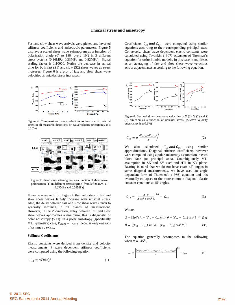
Fast and slow shear wave arrivals were picked and inverted

stiffness coefficients and anisotropic parameters. Figure 5

displays a scaled shear wave seismogram as a function of

polarization angle (00 to 1800 every 100) in 3 different

stress systems (0.16MPa, 0.33MPa and 0.52MPa). Signal

scaling factor is 1:10000. Notice the decrease in arrival

time for both fast (S1) and slow (S2) shear waves as stress

increases. Figure 6 is a plot of fast and slow shear wave

velocities as uniaxial stress increases.

Figure 4: Compressional wave velocities as function of uniaxial

stress in all measured directions. (P-wave velocity uncertainty is ± 0.15%)

Figure 5: Shear wave seismogram, as a function of shear wave

polarization () in different stress regime (from left 0.16MPa,

0.33MPa and 0.52MPa)

It can be observed from Figure 6 that velocities of fast and

slow shear waves largely increase with uniaxial stress.

Also, the delay between fast and slow shear waves tends to

generally diminish in all planes of measurement.

However, in the Z direction, delay between fast and slow

shear waves approaches a minimum; this is diagnostic of

polar anisotropy (VTI). In a polar anisotropy (specifically

VTI symmetry) case, ( ) ( ) because only one axis

of symmetry exists.

Stiffness Coefficients

Elastic constants were derived from density and velocity

measurements. P wave dependent stiffness coefficients

were computed using the following equation,

( ) (1)

Coefficients were computed using similar

equations according to their corresponding principal axes.

Conversely, shear wave dependent elastic constants were

calculated using Tsvankin (1997) extension of Thomsen’s

equation for orthorhombic models. In this case, it manifests

as an averaging of fast and slow shear wave velocities

across adjacent axes according to the following equation,

Figure 6: Fast and slow shear wave velocities in X (1), Y (2) and Z

(3) direction as a function of uniaxial stress. (S-wave velocity

uncertainty is ± 0.3%)

( ( ) ( )

)

(2)

We also calculated using similar

approximations. Diagonal stiffness coefficients however

were computed using a polar anisotropy assumption in each

block face (or principal axis). Unambiguously VTI

assumption in ZX and ZY axes and HTI in XY plane.

Bearing in mind that we do not have exact 450 angles in

some diagonal measurements, we have used an angle

dependent form of Thomsen’s (1986) equation and this

eventually collapses to the more common diagonal elastic

constant equations at 450 angles,

*

+

(3)

Where,

[

( ) ( )

] (3a)

[( )

( ) ] (3b)

The equation generally decomposes to the following

when ,

[( ( )

)

( )

]

(4)

© 2011 SEGSEG San Antonio 2011 Annual Meeting 21472147

Uniaxial stress and anisotropy

Similar assumptions were used to calculate

(HTI approximation was used for ). Figure 7 shows

compressional and shear wave dependent as well as

diagonal stiffness coefficients as a function of uniaxial

stress. Once again is low (Figure 7a) in comparison to

the rest due to the nature of the phenolic material being

used.

Figure 7: Stiffness coefficients as a function of uniaxial stress

Generally, within the limit of this experiment, all stiffness

coefficients tend to increase with uniaxial stress (except

that tend to remain constant). Diagonal elastic

constants (specifically ) remain largely

constant with changing stress but increases

significantly with stress. This may be due to an unknown

preferred orientation within the wave fabric of the phenolic

model.

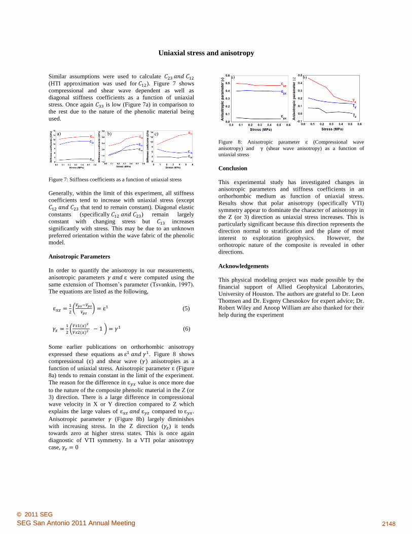
Anisotropic Parameters

In order to quantify the anisotropy in our measurements,

anisotropic parameters were computed using the

same extension of Thomsen’s parameter (Tsvankin, 1997).

The equations are listed as the following,

(

) (5)

( ( )

( ) ) (6)

Some earlier publications on orthorhombic anisotropy

expressed these equations as . Figure 8 shows

compressional ( ) and shear wave ( ) anisotropies as a

function of uniaxial stress. Anisotropic parameter (Figure

8a) tends to remain constant in the limit of the experiment.

The reason for the difference in value is once more due

to the nature of the composite phenolic material in the Z (or

3) direction. There is a large difference in compressional

wave velocity in X or Y direction compared to Z which

explains the large values of compared to .

Anisotropic parameter (Figure 8b) largely diminishes

with increasing stress. In the Z direction ( ) it tends

towards zero at higher stress states. This is once again

diagnostic of VTI symmetry. In a VTI polar anisotropy

case,

Figure 8: Anisotropic parameter (Compressional wave

anisotropy) and (shear wave anisotropy) as a function of

uniaxial stress

Conclusion

This experimental study has investigated changes in

anisotropic parameters and stiffness coefficients in an

orthorhombic medium as function of uniaxial stress.

Results show that polar anisotropy (specifically VTI)

symmetry appear to dominate the character of anisotropy in

the Z (or 3) direction as uniaxial stress increases. This is

particularly significant because this direction represents the

direction normal to stratification and the plane of most

interest to exploration geophysics. However, the

orthotropic nature of the composite is revealed in other

directions.

Acknowledgements

This physical modeling project was made possible by the

financial support of Allied Geophysical Laboratories,

University of Houston. The authors are grateful to Dr. Leon

Thomsen and Dr. Evgeny Chesnokov for expert advice; Dr.

Robert Wiley and Anoop William are also thanked for their

help during the experiment

© 2011 SEGSEG San Antonio 2011 Annual Meeting 21482148

EDITED REFERENCES

Note: This reference list is a copy-edited version of the reference list submitted by the author. Reference lists for the 2011

SEG Technical Program Expanded Abstracts have been copy edited so that references provided with the online metadata for

each paper will achieve a high degree of linking to cited sources that appear on the Web.

REFERENCES

Cheadle, S., J. Brown, and D. Lawton, 1991, Orthorhombic anisotropy: A physical seismic modeling

study: Geophysics, 56, 1603–1613, doi:10.1190/1.1442971.

Dellinger, J., and L. Vernik, 1994, Do traveltimes in pulse-transmission experiments yield anisotropic

group or phase velocities?: Geophysics, 59, 1774–1779, doi:10.1190/1.1443564.

Ebrom, D., J. A. McDonald, 1994, Seismic physical modeling: SEG Geophysics Reprint Series.

Pervukhina, M., D. Dewhurst, B. Gurevich, U. Kuila, T. Siggins, M. Raven, and H. M. N. Bolås, 2008,

Stress-dependent elastic properties of shales: Measurement and modeling: The Leading Edge, 27,

772–779, doi:10.1190/1.2944164.

Thomsen, L., 1986, Weak elastic anisotropy: Geophysics, 51, 1954–1966, doi:10.1190/1.1442051.

Tsvankin, I., 1997, Anisotropic parameters and P-wave velocity for orthorhombic media: Geophysics, 62,

1292–1309, doi:10.1190/1.1444231.

© 2011 SEGSEG San Antonio 2011 Annual Meeting 21492149