Unified Analysis of Discontinuous Galerkin Methods for Elliptic Problems Author(s): Douglas N. Arnold, Franco Brezzi, Bernardo Cockburn, L. Donatella Marini Source: SIAM Journal on Numerical Analysis, Vol. 39, No. 5 (2002), pp. 1749-1779 Published by: Society for Industrial and Applied Mathematics Stable URL: http://www.jstor.org/stable/4101034 Accessed: 02/05/2010 22:41 Your use of the JSTOR archive indicates your acceptance of JSTOR's Terms and Conditions of Use, available at http://www.jstor.org/page/info/about/policies/terms.jsp. JSTOR's Terms and Conditions of Use provides, in part, that unless you have obtained prior permission, you may not download an entire issue of a journal or multiple copies of articles, and you may use content in the JSTOR archive only for your personal, non-commercial use. Please contact the publisher regarding any further use of this work. Publisher contact information may be obtained at http://www.jstor.org/action/showPublisher?publisherCode=siam. Each copy of any part of a JSTOR transmission must contain the same copyright notice that appears on the screen or printed page of such transmission. JSTOR is a not-for-profit service that helps scholars, researchers, and students discover, use, and build upon a wide range of content in a trusted digital archive. We use information technology and tools to increase productivity and facilitate new forms of scholarship. For more information about JSTOR, please contact [email protected]. Society for Industrial and Applied Mathematics is collaborating with JSTOR to digitize, preserve and extend access to SIAM Journal on Numerical Analysis. http://www.jstor.org
Transcript
Unified Analysis of Discontinuous Galerkin Methods for Elliptic ProblemsAuthor(s): Douglas N. Arnold, Franco Brezzi, Bernardo Cockburn, L. Donatella MariniSource: SIAM Journal on Numerical Analysis, Vol. 39, No. 5 (2002), pp. 1749-1779Published by: Society for Industrial and Applied MathematicsStable URL: http://www.jstor.org/stable/4101034Accessed: 02/05/2010 22:41
Your use of the JSTOR archive indicates your acceptance of JSTOR's Terms and Conditions of Use, available athttp://www.jstor.org/page/info/about/policies/terms.jsp. JSTOR's Terms and Conditions of Use provides, in part, that unlessyou have obtained prior permission, you may not download an entire issue of a journal or multiple copies of articles, and youmay use content in the JSTOR archive only for your personal, non-commercial use.
Please contact the publisher regarding any further use of this work. Publisher contact information may be obtained athttp://www.jstor.org/action/showPublisher?publisherCode=siam.
Each copy of any part of a JSTOR transmission must contain the same copyright notice that appears on the screen or printedpage of such transmission.
JSTOR is a not-for-profit service that helps scholars, researchers, and students discover, use, and build upon a wide range ofcontent in a trusted digital archive. We use information technology and tools to increase productivity and facilitate new formsof scholarship. For more information about JSTOR, please contact [email protected].
Society for Industrial and Applied Mathematics is collaborating with JSTOR to digitize, preserve and extendaccess to SIAM Journal on Numerical Analysis.
SIAM J. NUMER. ANAL. ? 2002 Society for Industrial and Applied Mathematics Vol. 39, No. 5, pp. 1749-1779
UNIFIED ANALYSIS OF DISCONTINUOUS GALERKIN METHODS FOR ELLIPTIC PROBLEMS*
DOUGLAS N. ARNOLDt, FRANCO BREZZI , BERNARDO COCKBURN?, AND L. DONATELLA MARINIJ
Abstract. We provide a framework for the analysis of a large class of discontinuous methods for second-order elliptic problems. It allows for the understanding and comparison of most of the dis- continuous Galerkin methods that have been proposed over the past three decades for the numerical treatment of elliptic problems.
1. Introduction. In 1973, Reed and Hill [61] introduced the first discontinuous Galerkin (DG) method for hyperbolic equations, and since that time there has been an active development of DG methods for hyperbolic and nearly hyperbolic problems. Recently, these methods also have been applied to purely elliptic problems; examples are the original method of Bassi and Rebay [10], the variations studied in [23] and [22], and a generalization called the local discontinuous Galerkin (LDG) methods introduced in [41] and further studied in [33], [26], and [36]. Also in the 1970s, Galerkin methods for elliptic and parabolic equations using discontinuous finite elements were
independently proposed and a number of variants introduced and studied; see, for example, [50], [8], [70], [3], and [4]. These DG methods were then usually called interior penalty (IP) methods, and their development remained independent of the development of the DG methods for hyperbolic equations. In this paper, we present a detailed study of a class of DG methods for second-order elliptic problems which includes all the above-mentioned methods.
Next, we introduce the DG methods. For the sake of simplicity and easy presen- tation of the main ideas, we restrict ourselves to the model problem
(1.1) -Au = f in Q, u = 0 on OD,
where Q is assumed to be a convex polygonal domain and f a given function in L2 (Q). To place the DG methods into a common framework, we first rewrite the problem as a first-order system
S= Vu, -V-= f ins , u = 0 on 0Q.
*Received by the editors January 27, 2001; accepted for publication (in revised form) August 13, 2001; published electronically January 23, 2002.
http://www.siam.org/journals/sinum/39-5/38416.html tInstitute for Mathematics and Its Applications, University of Minnesota, Minneapolis, MN 55455
([email protected]). The work of this author was partially supported by National Science Foun- dation grant DMS-9870399.
IDipartimento di Matematica and I.A.N.-C.N.R., Via Ferrata 1, 27100 Pavia, Italy (brezzi@ dragon.ian.pv.cnr.it, [email protected]).
5School of Mathematics, University of Minnesota, Minneapolis, MN 55455 (cockburn@ math.umn.edu). The work of this author was partially supported by National Science Foundation grant DMS-9807491.
1749
1750 D. N. ARNOLD, F. BREZZI, B. COCKBURN, AND L. D. MARINI
Multiplying the first and second equations by test functions 7 and v, respectively, and integrating formally on a subset K of Q, we get
JK
a - dx =-
uV.Tdx KunK
T ds, K JK JOK
Sa
"
Vvdx
-
= f vdx + K
a f-nK vds, K JK J OK
where nK is the outward normal unit vector to OK. This is the weak formulation we shall use to define the DG methods.
Before doing that, we need to introduce the finite element spaces associated with the triangulation Th = {K} of the domain Q; as usual, we assume the triangles K to be shape-regular. We set
Vh:= {v GL2(Q) : VIKE P(K) VKE Th},
Eh := {TE[L2(Q)]2 TIK E(K) VK ETh},
where P(K) = Pp(K) is the space of polynomial functions of degree at most p > 1 on K and E(K) = [Pp(K)]2. Now, following Cockburn and Shu [41], we consider the following general formulation: Find uh e Vh and aEh E h such that for all K E Th we have
(1.2) Ia -*- dxx=-~V
U=K 72K r ds VT EE(K), JK JK UJ8laK
U
(1.3) ah Vvdx =K
f vdx + K 'nK vds Vv E P(K),
where the numerical fluxes 'K and UK are approximations to a = Vu and to u, respectively, on the boundary of K. To complete the specification of a DG method we must express the numerical fluxes &K and UK in terms of ah and Uh and in terms of the boundary conditions. This is why the above formulation is called the flux formulation. As we shall see, the choice of the numerical fluxes is quite delicate, as it can affect the stability and the accuracy of the method as well as the sparsity and symmetry of the stiffness matrix; cf. [41], [24], and [2]. In [2], we showed how to choose these numerical fluxes to recover virtually all the DG methods that have been proposed so far; see Table 3.1.
In this paper, we continue in several ways the work started in [2]. In order to put our work into proper perspective and give the reader an idea of the origins of the DG methods, we begin in section 2 with a brief overview of the historical development of the DG methods. Then, in section 3, we introduce a suitable functional setting and show how to go from the flux formulation (1.2)-(1.3) to a typical finite element formulation, called the primal formulation, which is obtained by eliminating the aux- iliary variable ah. Here, we relate the properties of consistency and conservativity of the numerical fluxes and the properties of consistency and adjoint consistency of the bilinear form of the primal formulation; see section 3.3. We make the discussion more concrete by looking more carefully at a few typical examples and then tabulate the flux choices and primal bilinear form for nine different methods which have appeared in the literature.
Next, we perform a unified error analysis of this model class of DG methods. In section 4 we first study the classical properties of consistency, boundedness, and
UNIFIED ANALYSIS OF DISCONTINUOUS GALERKIN METHODS 1751
stability typically used in finite element error analysis. Then, in section 5, we use them to obtain our error estimates. We begin with the fully stable and consistent methods. We show optimal error estimates in the energy norm, and we show that for adjoint- consistent methods an optimal L2-error estimate also can be achieved. Then, we relax the consistency conditions and show that optimal error estimates still can be obtained by forcing the penalty weights to be huge. This superpenalty technique, however, induces a significant increase in the condition number (see Castillo [25]), which could be a considerable source of difficulties. Finally, we relax the stability condition and consider two methods that do not have penalty terms and, as a consequence, are only weakly stable; they are the DG method of Baumann and Oden and the original DG method of Bassi and Rebay. The analyses of these methods are ad hoc but illustrate interesting theoretical techniques.
In section 6, we summarize the main features of the various methods (see Table 6.1), briefly comment on extensions in several possible directions, and conclude by discussing ongoing work and several open problems.
Notation. For convenience we list some of the most commonly used notation and the equations which best illustrate their definitions.
2. Historical overview. To put our work into proper perspective, we give a brief account of the development of the DG methods. We begin by considering penalty methods for elliptic equations.
2.1. Enforcing Dirichlet boundary conditions through penalties. The use of a penalty formulation for enforcing the Dirichlet boundary condition can be traced back to the late 1960s. Indeed, in 1968 Lions [56] considered the problem of solving elliptic problems with very rough Dirichlet boundary data; for example, -Aw = f in Q and w = g on
O•, where f is taken in L 2(Q) and g in H -1/2(09).
He regularized the above problem by replacing the Dirichlet boundary condition with the approximate boundary condition u + p-l1u/&n = g, where p was a large positive parameter. Lions proved that for each p > 0, there exists a unique solution u of the problem, and he proved that as ~ goes to infinity, this solution converges to the solution w of the original problem. The weak form of the regularized problem is to find u C H1(Q) such that
JVu - Vvdx+j at(u - g) v ds=f dx VvEH'(Q)
Note that the trial functions v do not satisfy the boundary conditions and that a penalty term has been added in order to force, in the limit as A tends to infinity, the satisfaction of the boundary conditions. In 1970, this approach was used by Aubin [5] in the framework of finite difference approximations of nonlinear problems. He proved that convergence to the exact solution can be obtained provided the penalty parameter p goes to infinity as the discretization parameter h goes to zero; in the linear case, convergence is achieved if p is of the order of h-'1+ for arbitrarily small c > 0. Finally, in 1973, the same approach was used in the finite element context by Babuika [6] for the case g = 0. For a finite element space using polynomials of degree p, the best error estimate obtained in [6] gives a rate of convergence of order
1752 D. N. ARNOLD, F. BREZZI, B. COCKBURN, AND L. D. MARINI
h(2p+1)/3 in the energy norm, provided that the penalty parameter /p is taken to be of the order of h-(2p+1)/3. The lack of optimality in the order of convergence is a direct consequence of the lack of consistency of the weak formulation. Indeed, note that the exact solution w does not satisfy the weak formulation of the regularized problem; instead, it satisfies
/Vw -Vvd- ~ w
vds + p(w - g) v ds= fvdx fn, an fr2
for all v E H1(Q). A different approach which still includes a penalty term but does not introduce any
consistency error was proposed in 1971 by Nitsche [58]. Nitsche's method determines an approximate solution Uh in a finite element subspace of H1 () such that B(uh, v) = f fv for all v in the same subspace. The bilinear form B(., -) is given by
B(u, v) :=Vu-Vvdx- j v ds - uds + puv ds a an aQn
for any weighting function p. Note that the second term of the bilinear form B, which arises naturally from an integration by parts, ensures the consistency of the method. On the other hand, the third term renders the discrete problem symmetric and hence ensures the property of adjoint consistency. Finally, the last term penalizes the departure of the trace of the approximate solution from the Dirichlet data g - 0 and is necessary to guarantee stability. Nitsche proved that if p is taken as j/1h, where h is the element size and r is a sufficiently large constant, then the discrete solution converges to the exact solution with optimal order in H1 and L2.
A third approach for weakly imposing the Dirichlet boundary condition is ob- tained by including all the terms in the bilinear form B(-, -) but reversing the sign of the third term. The resulting bilinear form B is no longer symmetric, but it has a favorable coercivity property, namely, B(u, u) > f IVul2, no matter how p > 0 is chosen. However, as we shall see, this method does not enjoy the adjoint consistency property mentioned above, a drawback that will adversely affect its L2 convergence properties.
2.2. The IP methods for elliptic problems. The IP methods arose from the observation that, just as Dirichlet boundary conditions could be imposed weakly instead of being built into the finite element space, so interelement continuity could be attained in a similar fashion. This makes it possible to use spaces of discontinuous piecewise polynomials for solving second-order problems (which could, for example, fa- cilitate adaptivity). In 1973, Babu ka and Z1imal [7] used interior penalties to weakly impose C1 continuity for fourth-order problems. Their bilinear form is analogous to the penalization technique used by Lions [56], Aubin [5], and BabuSka [6].
The natural generalization of Nitsche's method to second-order elliptic problems is stated in Wheeler's 1978 paper [70] on IP collocation-finite element methods; its weak formulation was motivated by the IP methods of Douglas and Dupont [50] and Baker [8]. That generalization of Nitsche's method is analyzed in detail for linear and nonlinear elliptic and parabolic problems in the 1979 thesis of Arnold [3], which is summarized in [4]. IPs of this sort were also used in 1977 by Baker [8] for imposing C1 interelement continuity on Co elements for fourth-order problems. In these, of course, it is the jump in the normal derivative that is penalized. In 1976, Douglas and Dupont [50] penalized the jump in the normal derivative of Co elements for second- order elliptic and parabolic problems, with the goal of enforcing a degree of continuity
UNIFIED ANALYSIS OF DISCONTINUOUS GALERKIN METHODS 1753
in some sense intermediate between CO and C1. This very same technique was then
applied to a nonlinear hyperbolic equation (arising in secondary oil recovery problems) in 1979 by Douglas et al. [49]. The IP term they introduced was devised to force the
approximate solution to become nearly C1 away from the shock discontinuity without
affecting the already existing artificial diffusion inserted in the method to properly deal with the shock.
Since the early 1980s, less attention has been paid to IP methods. This might be due to the fact that they were never proven to be more advantageous or efficient than classical conforming finite element methods; moreover, the difficulty in finding optimal values for the penalty parameters and the corresponding efficient solvers may have also contributed to this situation. Thus, the ease with which the IP methods handle
nonconforming meshes and varying-in-space polynomial degree approximations, which makes them ideally suited for hp-adaptivity, has never been fully exploited. Instead, techniques for enforcing continuity of the approximate solution in the framework of
hp-refinement were developed. Also, new methods that weakly enforce continuity across boundary elements were explored, such as the classical nonconforming and mixed methods [21], the mortar methods [20], [18], [19], and the cell discretization methods [52], [69].
In spite of this, IP methods have recently found a few new applications. Thus, in 1990, Baker, Jureidini, and Karakashian [9] enforced the divergence-free condition
pointwise inside each element for the Stokes system and used IPs to cope with the
resulting lack of continuity in the approximation of the velocity. In the same year, Rusten, Vassilevski, and Winther [65] used an IP method for second-order elliptic problems as part of a preconditioner for mixed methods. Finally, Becker and Hansbo
[17] and Dutra do Carmo and Duarte [48] recently used the IP approach as a way of
dealing with nonmatching grids for domain decomposition.
2.3. The DG methods for convection-dominated problems. On the other
hand, DG methods for the numerical treatment of nonlinear hyperbolic systems expe- rienced a vigorous development during the past 10 years due to a strong interaction with the ideas of numerical fluxes, approximate Riemann solvers, and slope limiters as developed for finite difference and finite volume methods for hyperbolic problems. Due to the nonlinear character of the equations, the DG methods had to be carefully crafted to achieve stability, high-order accuracy, and convergence to the so-called
entropy solution. This is the case of the Runge-Kutta DG (RKDG) methods de-
veloped by Cockburn and coauthors in [40], [39], [38], [34], and [42]; see also the introduction to the subject in [31], the short essay about the ideas used to devise DG methods for nonlinear hyperbolic equations in [32], and the recent review in [43]. Unlike the IP methods for elliptic problems, these DG methods have been proven to be clearly superior to the already existing finite element methods for hyperbolic conservation laws. A review of the development of DG methods up to May 1999 can be found in [37].
But the evolution of the DG methods did not stop there. The necessity of dealing with problems having a dominant convective part, as well as a nonnegligible diffusive part, prompted several authors to extend the DG methods to elliptic problems. Thus, in 1992 Richter [62] proposed a direct extension of the original DG method to linear convection-diffusion equations and proved that if the convection is dominant, that is, if the viscosity coefficients are of the order of the mesh size, the optimal order of convergence is k + 1/2 when polynomials of degree k are used.
For problems in which the diffusion might be dominant at least in some
1754 D. N. ARNOLD, F. BREZZI, B. COCKBURN, AND L. D. MARINI
regions of the domain, more precise handling of the second-order terms is necessary. Since mixed methods can handle elliptic operators very well and use a discontinu- ous approximation for the potential, they can be easily combined with discontinuous methods for advection. This idea was explored by several authors. In [44], [45], and
[46], Dawson combined the Raviart-Thomas mixed method for second-order operators with high-order Godunov methods for convection, giving rise to the so-called upwind- mixed methods (UMM) for advection-diffusion problems. See also [47] (where he and Aizinger obtained error estimates for arbitrary polynomial degree) and the applica- tion papers referenced there. In [28] and [29], Chen et al. used similar ideas for the discretization of the hydrodynamic and quantum hydrodynamic models for semicon- ductor device simulation. Specifically, they combined the Raviart-Thomas spaces for handling second-order elliptic operators with the discontinuous approximations of the RKDG method. See also the review in [35]. Finally, Lomtev, Quillen, and Karniadakis [57] used the DG-space discretization method to handle the convective part of the compressible Navier-Stokes equations combined with a mixed method to approximate the diffusive part of the equations.
All the above methods used discontinuous approximation only for the convec- tive terms and mixed methods for second-order elliptic operators. This enforced the continuity of the normal component of the approximation to a = Vu across the el- ements. It was only in 1997 that completely discontinuous approximations for both u and a = Vu were used by Bassi and Rebay [10]. Indeed, these authors used the discretization ideas of the RKDG methods to introduce a new DG method for the compressible Navier-Stokes equations. In 1998 Cockburn and Shu [41] introduced the so-called local discontinuous Galerkin (LDG) methods for transient nonlinear convection-diffusion problems by generalizing the original DG method of Bassi and Rebay; see also Cockburn and Dawson [33] for their extension of the LDG methods to problems with quite general second-order terms; Castillo et al. [27] for their analysis of the hp version of the LDG method in one space dimension; and Shu [66] for his review on the different discretizations of second-order terms by means of DG methods.
Around the same time, Baumann and Oden [15], [14] introduced another DG method for diffusion problems. Their approach is analogous to the third approach described earlier for weakly enforcing Dirichlet boundary conditions; it results in a coercive bilinear form even when the penalty parameter vanishes but, on the other hand, the bilinear form is not symmetric even for symmetric problems, and so the method is not adjoint consistent.
2.4. A first attempt to unify the DG methods. In recent years, several authors were struck by the similarities between the recently introduced DG methods and the IP methods, and began applying to the former the techniques of analysis developed earlier for the latter. Thus Brezzi et al. [22], [23] studied several variations of the original method of Bassi and Rebay; Oden, Babuika, and Baumann [59] stud- ied the DG method of Baumann and Oden; Riviere and Wheeler [63] and Riviere, Wheeler, and Girault [64] analyzed several variations of the DG method of Baumann and Oden; Becker and Hansbo [16] proved a posteriori estimates for the IP approach to convection-diffusion problems; Houston, Schwab, and Siili [68], [67], [54] synthe- sized the elliptic, parabolic, and hyperbolic theories by extending the analysis of DG methods to partial differential equations with a nonnegative characteristic form; and, more recently, Castillo et al. [26] and Cockburn et al. [36] studied the LDG method as applied to purely elliptic problems in arbitrary and Cartesian meshes, respectively.
The presentation of all these methods, however, followed two main styles.
UNIFIED ANALYSIS OF DISCONTINUOUS GALERKIN METHODS 1755
Indeed, the methods inspired by the original IP methods were typically presented in their primal formulation as, for instance, in [15], [14], [59], [68], [67], and [54], while the methods inspired by the finite volume techniques for hyperbolic problems were presented in terms of suitably chosen numerical fluxes as, for instance in [10], [41], [33], even if the analysis was accomplished by shifting to a suitable associated bilinear form.
In a previous paper [2], we made a first attempt to unify these two families and succeeded in recasting all of the above-mentioned methods within a single framework in order to better understand the connections among them. In particular, it was shown that the methods of the first family, based on the choice of the bilinear form, could be obtained as special cases of the second family simply by choosing the proper numerical fluxes; see Table 3.1. Since some of the new DG methods (of the second family) have inherited the carefully crafted technique of defining numerical fluxes achieved for nonlinear hyperbolic problems, it is plausible that the resulting DG methods for elliptic problems could be more efficient than the old ones, possibly after some suitable refinement.
In this paper, we complete the work started in [2]. To do that, we start by relating the flux and primal formulations.
3. The flux and primal formulations. In this section, we relate the flux for- mulation (1.2)-(1.3) of a DG method to its primal formulation (3.10). We show that consistency and conservation properties of the numerical fluxes are reflected in consis- tency and adjoint consistency of the primal formulation. We introduce nine examples of DG methods which have appeared in the literature-some derived originally in a flux formulation, others in a primal formulation-and present the numerical fluxes and primal form for all of them.
3.1. Traces and numerical fluxes. We begin by introducing an appropriate functional setting. We denote by H1 (Th) the space of functions on Q whose restriction to each element K belongs to the Sobolev space H'(K). Thus, the finite element spaces Vh and Eh are subsets of H (Th) and [H (Th)]2, respectively, for any 1. The traces of functions in H1(Th) belong to T(F) := IIKThL2(OK), where F is used to denote the union of the boundaries of the elements K of Th. Functions in T(F) are thus double-valued on F0 := F \ 0Q and single-valued on 0Q. The space L2(F) can then be identified as the subspace of T(F) consisting of functions for which the two values coincide on all internal edges.
We take the scalar numerical flux U = (UK)KeTh and the vector numerical flux S ('K)KETh to be linear functions
(3.1) --+ H()•
T(F), & H2('h) x [Hl(7h)]2 -+ [T(F)]2.
In fact, only the normal component of 0 plays a role in the DG method; see (1.3). We could, without loss of generality, insist that a be directed normally on each edge, but for simplicity we do not.
The properties of consistency and conservativity of the numerical fluxes are im- portant in the analysis of the DG methods. We say that the numerical fluxes are consistent if
Svlr, (v, w7) - vlr, whenever v is a smooth function satisfying the Dirichlet boundary conditions. We say that the numerical fluxes Ui and & are conservative if '( - ) and ( ., ?
), respectively, are
1756 D. N. ARNOLD, F. BREZZI, B. COCKBURN, AND L. D. MARINI
single-valued on F. The term conservative comes from the following useful property, which holds whenever the vector flux 8 is single-valued: If S is the union of any collection of elements, then, taking v in (1.3) to be identically one in S and adding over the elements K contained in S, we get
(3.2) sf
dx + l "rns
ds = 0.
Next, we introduce some trace operators that will help us to manipulate the numerical fluxes and obtain the primal formulation. For q E T(F), we define the average {q} and the jump q J of q on FO as follows. Let e be an interior edge shared by elements K1 and K2. Define the unit normal vectors nl and n2 on e pointing exterior to K1 and K2, respectively. With qi :=
qlaKi we set
1
{q} -- (q +q2), q = qlnlq 2n2 on e Eh, 2
h
where S' is the set of interior edges e. For Ge [T(F)]2 we define P1 and 2 analogously and set
{( •1
P2), (1 1 nl + P2 n2 on e c . 2
Notice that the jump [ q ] of the scalar function q is a vector parallel to the normal, and the jump [ V of the vector function V is a scalar quantity. The advantage of these definitions is that they do not depend on assigning an ordering to the elements Ki. For e E Sh, the set of boundary edges, each q E T(F) and V E [T(r)]2 has a uniquely defined restriction on e; we set
q = qn, {f}-=•
oneE 'h,
where n is the outward unit normal. We do not require either of the quantities {q} or ~ p p on boundary edges, and we leave them undefined. In short,
{ }: T(F) --+ L2(FO), [I - : T(F)-+ [L2()]2,
{ } : [T(F)]2 -+ [L2(F)]2, . -: [T(F)]2 -+ L2(F0). 3.2. The primal formulation. With the notation introduced above, we are
ready to obtain the primal formulation. If, in (1.2)-(1.3), we add over all the elements, we obtain
Jh' Tdx-=-jUhVh.Tdx?+ ZjUKnK'Tds
VT EEh, 1?2J? K E Th ' K
hoh - Vhv d = f vdx?+ S ' f-K vds Vv EVh,
Q J KEThaK
where Vhv and Vh T7 are the functions whose restriction to each element K E Th are equal to Vv and V - 7, respectively.
To deal with the sums of the form KErh faK qKPO K K nK
ds, we use the average and jump operators. A straightforward computation shows that for all q E T(F) and for all E [T(F)]2,
(3.3) qKK " nK ds
- q {} ds
+f {q}[p]]ds. K E Th o
UNIFIED ANALYSIS OF DISCONTINUOUS GALERKIN METHODS 1757
After a simple application of this identity, we get
(3.4) ja - -dx- - UVh -TTdx+ (jU-[{}+ds-+j{U}l[T] ds VT CzEih, Jo Jo JCfr Jr]O
(3.5) jU/-iVhv dx-j{ }vds-jV{v}-jfyvdx VvC Vi. JQ fir- Jro CQ
Now, we express ah solely in terms of Uh. To do that, we use another identity. If in (3.3) we take q equal to the trace of v, and p equal to the trace of T, we obtain, for all T E
[H1(Th)]2 and v E H1(Th), the integration by parts formula
Taking 7 = Vhv in the identity (3.7) we may then rewrite (3.5) as follows:
(3.10) Bh(Uh,
v) = fv dx Vv Vh,
where
(3.11) Bh(Uh,V)'
:= VhUh.
-Vhvdx+ ([+ J (-uhl]
{Vhv} -
{P}'-[v])ds +
o ({
- }[)a, v
- g{v}) ds.
For any functions Uh E H2(Th) and v E H2(Th), (3.11) defines Bh (Uh, v), with the understanding that 7 = ?(uh) and & = &(uh,a (Uh)), where the map uh / ah (Uh) is given by (3.9). The form Bh : H2(Th) x H2(Th) --+ R is bilinear and, if (uh, ah) E Vh x Eh solves (1.2)-(1.3), then uh solves (3.10) and ah is given by (3.9). We call (3.10) the primal formulation of the method and call the bilinear form Bh(., -) the primal form.
3.3. Consistency and conservation. Let u solve the boundary value problem (1.1). By the integration by parts formula (3.6), we have for any v E H2(Th) that
j Vhu- Vhvdx=
- Auvdx + j{Vhu} - [v ds +
jVhiuL {v} ds,
1758 D. N. ARNOLD, F. BREZZI, B. COCKBURN, AND L. D. MARINI
and since {u} = u, u] = 0, {Vhu} = Vu, IVhU] = 0, and -Au = f, we have
where U7 = ?4(u), ' = &(u, ah(u)). If the numerical flux i is consistent, i.e., ~(u) = ufr,
then [i = 0 and {I} = u on F. Then (3.9) implies that crh(u) = Vu. If the vector numerical flux ' is also consistent, we then get that [I] = 0, {&} = Vu on F. Inserting these relations in (3.12) we conclude that
(3.13) Bh(U, v) = f vdx.
Thus, if the numerical fluxes are consistent, (3.13) holds for all test functions v E H2 (Th). This implies that the primal formulation is consistent, which is defined to mean that (3.13) holds, at least for all v E Vh; equivalently, in view of (3.10) it means that Galerkin orthogonality holds:
(3.14) Bh(u - Uh, V) = 0 Vv E Vh.
In fact, using the density of the range of the trace operator, it is not difficult to reverse the above argument and show that if (3.13) holds for all v E H2(Th), then the numerical fluxes must be consistent. We do not know of any DG methods for which (3.13) holds for all v E Vh but not for all v E H2(Th). Thus consistency of the numerical fluxes is practically equivalent to consistency of the primal formulation.
Now let 0 solve
(3.15) -AO = g in 0, ,
= 0 on oQ.
If
(3.16) Bh(v, ) = v g dx Jo2
for all v E H2(Th), then we say that the primal form is adjoint consistent. (The boundary value problem (3.15) is the adjoint of the problem we started with, which in this case is again the Dirichlet problem for the Poisson equation, because that problem is self-adjoint.) Since c H2 (Q), we obtain {Jb} = V, 1J] = 0, {V1 } = V4), and
[ VO I = 0. Therefore
SVhV - Vhdx=j v g dx +
jFrv •- Vds,
and then with (3.11) we get
Bh(v,4) - vgdx + j[(v)] -
V4dsj-
ro(vah(v))J]ds. Now suppose that the numerical fluxes are conservative. This means that [ =- 0
and [ & = 0. Thus, conservativity of the numerical fluxes implies adjoint consistency. Conversely, if either [i i(v) ] or [~'(v, h(v)) does not vanish for some v, then there is a smooth function 4 for which (3.16) does not hold.
UNIFIED ANALYSIS OF DISCONTINUOUS GALERKIN METHODS 1759
3.4. Examples of DG methods. A simple and natural choice of numerical fluxes is
S= {Uh} onF , = 0on •O, and i=-{ah}onF.
This is the choice proposed by Bassi and Rebay in [10]. With this choice of ~', we have {f - Uh} = 0 and [;- Uh ] = - Uh I, so (3.9) gives
(3.17) ah VhUh + r([IUh 1).
Therefore
(3.18) J{&} - jvjdsh={Vu} * -v]ds - jr( U(uh
)r(?v]) dx,
where we used the fact that r([ Uh ]) e Eh and the definition (3.8) of r in the last
step. Substituting in (3.11) we obtain the following primal form for the method of
Bassi-Rebay [10]:
Bh(Uh, V) = ][VhUh Vhv + r(?Uh )r([v ]) dx
-
({VahUh}? -v]+ [[Uh]-
{Vhv})ds.
As a second example, we consider the classic IP method. This was originally proposed as a primal formulation, with
(3.19)
Bh(uh, v) = VahUh. Vhvdx - (?uh {VhV } + {VhUh} [v) ds + a(u, v), Jo Jr
where
(3.20) ad (uh, v) = p Uh [v ds Jr
is the IP or stabilization term with the penalty weighting function p : F -+ R given by ,eh 1 on each e E Sh with 7e a positive number. It is easy to see that this method arises as well from a proper choice of fluxes,
(3.21) f={uh} onFo, =0=Oon&Q8, and o= {Vhuh}- ajj([Uhl) on F,
where aj(?p) is simply p?, i.e., rleheIp on e. Again we have ah as in (3.17), while instead of (3.18) we get
(3.22) j{'ll} -
[vds= jVhUh} jvds -
aj([Uh]) -
?v ds,
and (3.19) follows by substituting (3.22) in (3.11). The vector flux for the IP method contains the jump term aj(([uh 1) which is
equal to 7,eh1 Uh 1 on e. An alternative jump term is obtained using the lift operator re: [Ll(e)]2 -- h given by
(3.23) re (p) . rdX = j- - {T} ds V E•
, IL'(e)]2. JO Je
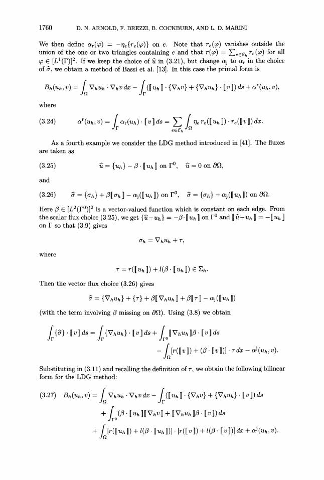
1760 D. N. ARNOLD, F. BREZZI, B. COCKBURN, AND L. D. MARINI
We then define a,(rp) = -rie{re(op)}
on e. Note that re,(Q) vanishes outside the union of the one or two triangles containing e and that r(?o) =
ZeE•• re (W) for all
~ [Ll(r)]2. If we keep the choice of U in (3.21), but change aj to ar in the choice of a, we obtain a method of Bassi et al. [13]. In this case the primal form is
Bh(uh, v) =j VhUh - Vhv dx - ([Uh I {Vhv}+{Vu} -I v ]) ds +
a-r(Uh,
V),
where
(3.24) aor(Uh,
V) j ar(u) - v]dS = E re((-Uhl)
-.re(IV]) dx.
eEEh
As a fourth example we consider the LDG method introduced in [41]. The fluxes are taken as
(3.25) u= {Uh} - P-. Uh ] on Fo, U~= 0 on 9Q,
and
(3.26) ' = {ah} + P3 ah ] - aj(lUh ]) on Fo, = {ah} - aj(I[uh ]) on (0.
Here3 E [L2 (F)]2 is a vector-valued function which is constant on each edge. From the scalar flux choice (3.25), we get {--uh} =
--3 [Uh ] on r and [--Uh ] = -[Uh ]
on F so that (3.9) gives
Cah = VhUh + 7,
where
7 = r(Uh ) + 1( - jIUh 1) E Eh.
Then the vector flux choice (3.26) gives
S= {VhUh} + {7T} + P0VhUhI + P3[TI - aj([Uh])
(with the term involving / missing on 0S). Using (3.8) we obtain
{} v]ds= j{Vhuh}. -[v]ds+ If[VhUh13- [v]Ids
- [r(v ]) + (13. v )]).
dx - aj (Uh, v).
Substituting in (3.11) and recalling the definition of 7, we obtain the following bilinear form for the LDG method:
Babubka-Zliimal [7] g + aJ (w, v) Brezzi et al. [23] g + ar(w, v)
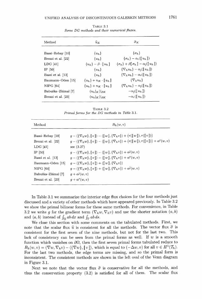
In Table 3.1 we summarize the interior edge flux choices for the four methods just discussed and a variety of other methods which have appeared previously. In Table 3.2 we show the primal bilinear forms for these same methods. For convenience, in Table 3.2 we write g for the gradient term (VhW, Vhv) and use the shorter notation (a, b) and (a, b) instead of fo ab dx and fr ab ds.
We close this section with some comments on the tabulated methods. First, we note that the scalar flux U' is consistent for all the methods. The vector flux
' is consistent for the first seven of the nine methods, but not for the last two. This lack of consistency can be seen from the primal forms as well. If w is a smooth function which vanishes on OR2, then the first seven primal forms tabulated reduce to
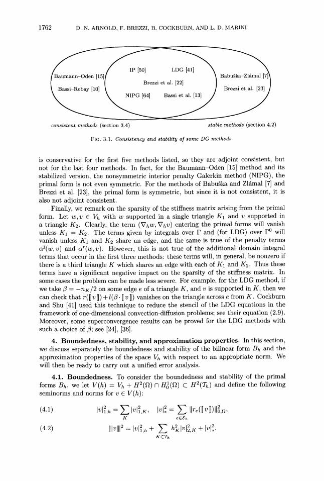
Bh(W, v) = (VW, VhV)- ({Vw}, V] ), which is equal to (-Aw, v) for all v E H1(Th). For the last two methods, the edge terms are missing, and so the primal form is inconsistent. The consistent methods are shown in the left oval of the Venn diagram in Figure 3.1.
Next we note that the vector flux & is conservative for all the methods, and thus the conservation property (3.2) is satisfied for all of them. The scalar flux
1762 D. N. ARNOLD, F. BREZZI, B. COCKBURN, AND L. D. MARINI
IP [50] LDG [41] Baurnann-Oden [15][ Babuika-Zlamal [7]
Brezzi et al. [22] Bassi-Rebay [10] Brezzi et al. [23]
FIG. 3.1. Consistency and stability of some DG methods.
is conservative for the first five methods listed, so they are adjoint consistent, but not for the last four methods. In fact, for the Baumann-Oden [15] method and its stabilized version, the nonsymmetric interior penalty Galerkin method (NIPG), the
primal form is not even symmetric. For the methods of Babugka and Zlamal [7] and Brezzi et al. [23], the primal form is symmetric, but since it is not consistent, it is also not adjoint consistent.
Finally, we remark on the sparsity of the stiffness matrix arising from the primal form. Let w, v E Vh with w supported in a single triangle K1 and v supported in a triangle K2. Clearly, the term (VhW, Vhv) entering the primal forms will vanish unless K1 = K2. The terms given by integrals over F and (for LDG) over F0 will vanish unless K1 and K2 share an edge, and the same is true of the penalty terms aj (w, v) and ar (w, v). However, this is not true of the additional domain integral terms that occur in the first three methods: these terms will, in general, be nonzero if there is a third triangle K which shares an edge with each of K1 and K2. Thus these terms have a significant negative impact on the sparsity of the stiffness matrix. In some cases the problem can be made less severe. For example, for the LDG method, if we take 0 = -nK/2 on some edge e of a triangle K, and v is supported in K, then we can check that r([ v 1) + 1(3- I v ) vanishes on the triangle across e from K. Cockburn and Shu [41] used this technique to reduce the stencil of the LDG equations in the framework of one-dimensional convection-diffusion problems; see their equation (2.9). Moreover, some superconvergence results can be proved for the LDG methods with such a choice of 3; see [24], [36].
4. Boundedness, stability, and approximation properties. In this section, we discuss separately the boundedness and stability of the bilinear form Bh and the
approximation properties of the space Vh with respect to an appropriate norm. We will then be ready to carry out a unified error analysis.
4.1. Boundedness. To consider the boundedness and stability of the primal forms Bh, we let V(h) = Vh + H2(Q) n H,(Q) C H2(Th) and define the following seminorms and norms for v E V(h):
(4.1) ]IVh =
vII,K, 2 =E I Il K eEh
(4.2) 11hv]]2 = v,h + h2Kiv,K + V2.
KETh
UNIFIED ANALYSIS OF DISCONTINUOUS GALERKIN METHODS 1763
The norm (4.2) is the natural one for obtaining boundedness of the bilinear form Bh. On the other hand, the weaker norm
(4.3) v (IVh + V1)1/2
is the natural one for analyzing the stability of many DG methods. Restricted to v E Vh, these two norms are equivalent, as is evident from a local inverse inequality. We also remark that both (4.2) and (4.3) define norms, not just seminorms, on V(h). Indeed, the discrete Poincard inequality given in [4, Lemma 2.1], together with the second inequality of (4.5) below, implies the existence of a constant C for which
I|v o < C(v i,h + v12V)1/2 Vv E V(h). We now show that for many DG methods, including all those listed in Table 3.2,
the primal bilinear form Bh is bounded with respect to the norm III | 11, that is,
(4.4) Bh(w,v) ? CbIIIW • IIIv 11 Vw, v E V(h). We show this by bounding each of the various terms that appear in the table.
Obviously we have (VhW, VhV) < Cw|ll,hlVll,h and, from the definition (3.24), ar (W,) ?
(supe ~e)WI*l Iv*. Now, by the definition of re, (3.23), and after using inverse inequalities as in [22],
where he denotes the length of the edge e and the constants C1 and C2 depend only on the minimum angle of the decomposition and the polynomial degree p. Since 1 v vanishes for v E H2 (Q) no H(Q), we can apply the above inequalities with p = [v for any v E V(h), and then summation over the edges e then gives
(4.5) Clvl2 < h-jll[vlC2Ve < C2Vl Vv E V(h). eEgh
It thus follows that aiJ(w, v) C2(supe le)lw *,vL, for w, v E V(h) and also that the
term fro[W ]w. I-v I ds, which occurs in the primal form of the LDG method (3.27), is bounded by Clwl,lvl. with C = supe he, 113L L(e). Next we recall that for W E [L2(F)]2, re (p) vanishes on the interior of any triangle K unless e is one of the edges of K. Therefore
2
l 2
,() <3 e Ie () ,, eEFh OQ eCEh
whence
(4.6) ]r([]) ll~, 31v.2
Vv E V(h), and so f r([w ]) - r([v ]) dx <
31,l 1 v|, for w, v E V(h).
Next we bound the terms fr{Vhw}. v ds and fr[w ].- {VhV} ds which arise for the first seven of the tabulated methods. We begin by noting that if w E H2 (K) and e is an edge of K, we have [4, eq. (2.5)],
(4.7)< - C(h w wK
e2 n 0, 1,K + hGlwlK)e O,e
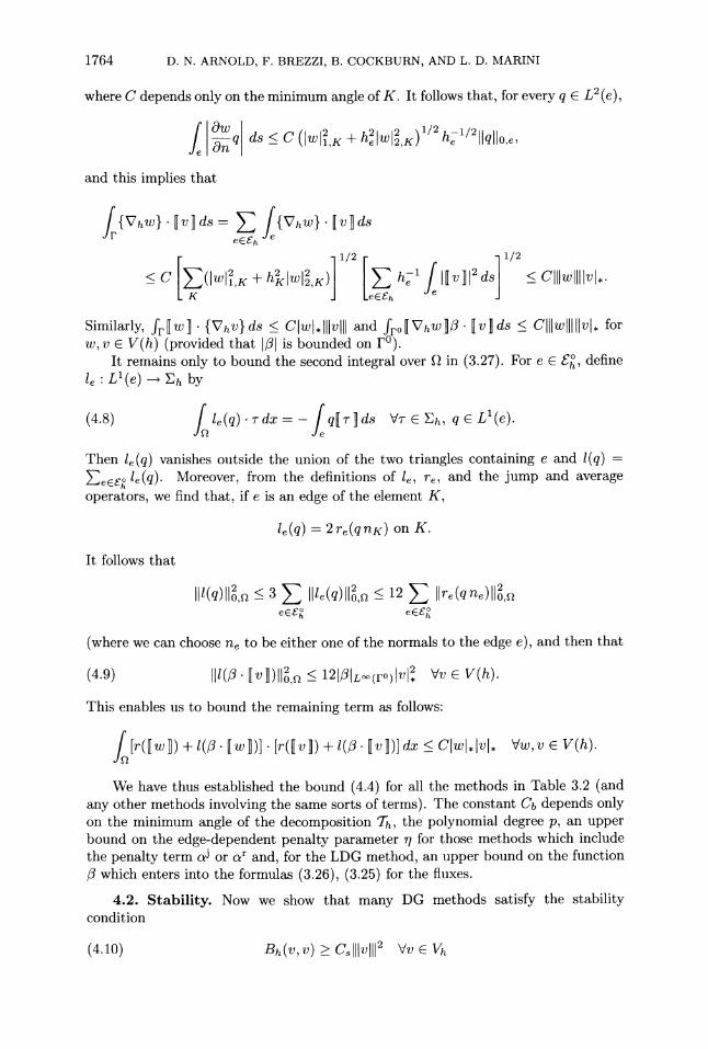
1764 D. N. ARNOLD, F. BREZZI, B. COCKBURN, AND L. D. MARINI
where C depends only on the minimum angle of K. It follows that, for every q E L2(e),
w dw q ,K)1/2
d C/2wIh ,e e n 1 e 2
and this implies that
jr{Vhw} I[vlds= i{Vhw}- [vL ds
SeESh C
1/2 1/2
< c (Iw|lK 2K ,K E -1 IU
2 ds < l w Ul. L K
+ Kl21K)h v deESh e
fl , Similarly, fr[w -. {Vhv}ds < Cw|,*II|vI|| and fro[w VhW I [v]ds < c|wlllw||vl* for w, v E V(h) (provided that 131 is bounded on F0).
It remains only to bound the second integral over Q in (3.27). For e E E, define le : L'(e) -- Eh by
(4.8) le(q). -dx = - q[T]ds VT E Eh, q E L(e).
Then le (q) vanishes outside the union of the two triangles containing e and 1(q) =
-eEE•, le(q). Moreover, from the definitions of le, re, and the jump and average
operators, we find that, if e is an edge of the element K,
le (q) = 2 re(q nK) on K.
It follows that
I|l(q) l~,2
< 3 • 1le(q) , <12 j
re(qne)l,
(where we can choose ne to be either one of the normals to the edge e), and then that
(4.9) IIl(P - [vj)ll2,2 <
121|ILL-O(o)lvI Vv E V(h).
This enables us to bound the remaining term as follows:
f r([w ) + 1(-[
w])?] [r(v]) + 1(/3. [v)] dx C |lwllv Vw, ve V(h).
We have thus established the bound (4.4) for all the methods in Table 3.2 (and any other methods involving the same sorts of terms). The constant Cb depends only on the minimum angle of the decomposition Th, the polynomial degree p, an upper bound on the edge-dependent penalty parameter r7 for those methods which include the penalty term aj or ar and, for the LDG method, an upper bound on the function
3 which enters into the formulas (3.26), (3.25) for the fluxes.
4.2. Stability. Now we show that many DG methods satisfy the stability condition
(4.10) Bh(v, v) > Clllv~211 Vv E Vh
UNIFIED ANALYSIS OF DISCONTINUOUS GALERKIN METHODS 1765
with C, a positive constant. With reference to Tables 3.2 and 3.1 we may write, for all nine tabulated methods,
Bh(v, v) = IvllhVlO,' + a(v, v) + b(v, v), where a is either ar,
ao, or zero depending on whether the flux 'K for the method
contains ar, aj, or neither, and b gathers up all the remaining terms of the primal form. From the bounds we obtained in the last section, we know that Ib(v, v)l < CIIIvllllvl for some constant C and all v E V(h).
When present, the penalty term ar or ai contributes to the stability of the method. For ar, we obtain immediately from (3.24) and the definition of ( I, in (4.1) that
(4.11) ar(v,v) 2 rVoIvl Vv E Vh,
where ro0 - infe Tie. In view of (4.5) we have for ai that
(4.12) ai(v, v)2 ClTIOIvl2 Vv E Vh.
Thus, for methods involving a penalty term,
Bh(V, v) 2 IV,h + Co7o0VI - CvIIIVI* V E Vh V, where Co equals 1 or C1, depending on whether the penalty term is ar or ai, and where C depends on the angle condition, polynomial degree and, in the case of the LDG method, a bound for the coefficient P. We may then use the arithmetic-geometric mean inequality (2ab < a2E + b2/E) on the last term, and then the equivalence of the norms (4.2) and (4.3), to show that (4.10) holds for large enough r0o. Thus all the methods considered which include a penalty term ar or aj are stable, assuming that the stabilizing coefficients %re are chosen sufficiently large. This includes seven of the nine methods listed in the tables. The remaining two methods, that of Baumann and Oden [15] and that of Bassi and Rebay [10], are not stable, as will be discussed below. The stable methods are indicated in the right oval of the Venn diagram in Figure 3.1.
While the argument just presented establishes stability when the rie are chosen sufficiently large, it does not make clear just how large they must be taken. For some methods, a precise sufficient condition can be obtained by a sharper analysis. To this end we define R(v) = r([v1) and Lf(v) = l(0. [v Iv, so
(4.13) jR(v) rTdx = - [v] {T} ds, L(v) . rdx = -
f•3.v
]?-i ds
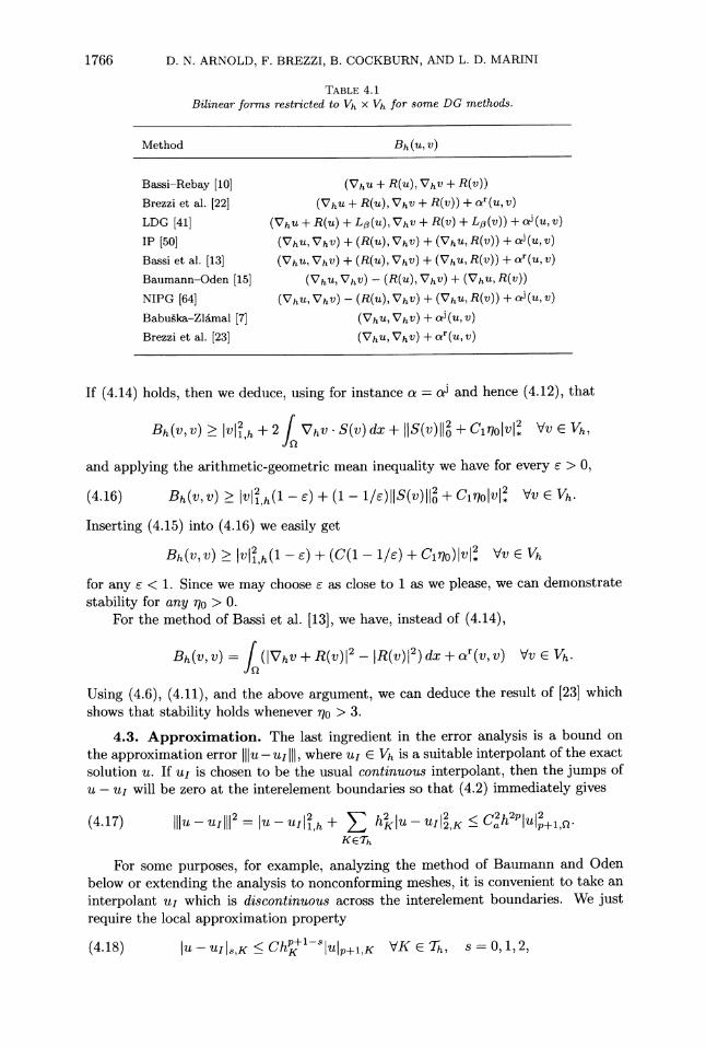
for all T E Eh. We may use this notation to give simpler expressions of the primal form when both arguments belong to Vh. See Table 4.1.
From the table we see that five of the methods-all but the unstable methods Bassi-Rebay [10] and Baumann-Oden [15], the IP method, and the method of Bassi et al. [13]-satisfy
(4.14) Bh(v, v) > Vh + S(v)ldx+ a(v, v) Vv E Vh,
where S(v) stands for a linear combination of the terms R(v) and Lp(v) and a is either ar or aj. From (4.6) and (4.9) we know that
(4.15) IIS(v)l0lo, < Cl•v*.
1766 D. N. ARNOLD, F. BREZZI, B. COCKBURN, AND L. D. MARINI
TABLE 4.1 Bilinear forms restricted to Vh x Vh for some DG methods.
Using (4.6), (4.11), and the above argument, we can deduce the result of [23] which shows that stability holds whenever q7o > 3.
4.3. Approximation. The last ingredient in the error analysis is a bound on the approximation error IIlu - ulll, where
ui E Vh is a suitable interpolant of the exact
solution u. If ul is chosen to be the usual continuous interpolant, then the jumps of u -
ui will be zero at the interelement boundaries so that (4.2) immediately gives
(4.17) I|u - u/I|2
= U - UIl,h •+
I h Iu - 2
Ul,K • Ch2 2
K ETh
For some purposes, for example, analyzing the method of Baumann and Oden below or extending the analysis to nonconforming meshes, it is convenient to take an
interpolant ul which is discontinuous across the interelement boundaries. We just require the local approximation property
(4.18) u - uIls,K ChPK+1-sIup+1,K VK E Th, s = 0, 1,2,
UNIFIED ANALYSIS OF DISCONTINUOUS GALERKIN METHODS 1767
where C depends only on p and the minimum angle of K. Using a discontinuous ui forces us to take into account the term u - ui1 in (4.2). For this, we first use (4.5) to obtain
(4.19) lu - tI|2 K ll -UI-Ih+ 3E hIU - U II2,K +-1 SC h lUU-I -
l,e. KETh eEEh
Next, we recall that (see, e.g., equation (2.4) of [4])
(4.20) IIvll,e < C(h|lllVI 2,K + he ,K) Vv H(K)
where K is a generic triangle having e as an edge, and C is a constant depending only on the minimum angle of K. Finally, using (4.19) and (4.20), we obtain
(4.21)
llu - u 1112 < C (-
U ,h + hlu - ull ,K + h211u - _ U ,K)
KETh KETh
and from (4.18) and (4.21) we have again
(4.22) Ilu - uzi l < CahPlulp+1,Q. From now on, when speaking about interpolants we shall always assume that they satisfy (4.18), and hence (4.22).
5. Error estimates. We now prove error estimates for the DG methods by using the properties of consistency, boundedness, stability, and approximation just discussed. First, we consider methods that are consistent, adjoint consistent, and
stable; in this case, optimal error estimates follow in the standard way. Then we study methods that are not consistent and show how to overcome their lack of consistency (and obtain optimal error estimates) by means of a superpenalty procedure. This is the case for the two pure penalty methods at the bottom of Table 3.1, as well as the variant of the NIPG method (consistent but lacking adjoint consistency) which is considered in [64]. Finally, we consider the two unstable methods, Bassi-Rebay [10] and Baumann-Oden [15]. These methods do not have a penalty term and their more subtle convergence behavior requires a finer analysis.
5.1. Stable and completely consistent methods. Methods that are com-
pletely consistent and stable can be shown to converge with optimal order with respect to the norm III III in the standard way. Indeed, let uI be a piecewise Pp interpolant of
u which satisfies (4.18). Then, using stability (4.10), consistency (3.14), boundedness
(4.4), and the approximation property (4.22), we have
Cs Iu - uh 1112 Bh(UI - uh, UI - Uh) = Bh(UI - u, UI - uh)
<CbI luI - Hlll III - hHll < Ch lulp+l,,olluHI - Uh ll. Hence, the triangle inequality gives the optimal estimate
IIIU - Uh ll < ChP|lup+i,,. Next, we show that when the adjoint consistency condition (3.16) holds, we can
obtain optimal order L2-error estimates by using the standard duality argument. As
usual, we define the auxiliary function 0 as the solution of the adjoint problem
(5.1) -A = u - Uh in Q, 0 = 0 on o9Q
1768 D. N. ARNOLD, F. BREZZI, B. COCKBURN, AND L. D. MARINI
and write, in view of the adjoint consistency condition (3.16),
(5.2) Bh(V, ) = (U - Uh, v) Vv E V(h). We take V) to be a piecewise linear interpolant of 0. Then, taking v= u - Uh in (5.2) and using the consistency condition (3.14), we obtain
As Q is convex, elliptic regularity gives 1012,Qn ? CrU - Uhl 0o, with Cr depending only on the domain Q. Hence, we get the optimal estimate
IIu - Uh1lo0,a ? Chp+llul p+l,.
For the NIPG method, the above argument fails because the method does not
satisfy the adjoint consistency condition (3.16). In fact, this method does not achieve
optimal order convergence in L2. However, as we shall see in a moment, the optimal rate of convergence in the L2-norm can be recovered if we use a penalty term similar to the one used for pure penalty methods.
Finally, we remark that the error analysis for stable and consistent methods can be extended to the case of nonconforming meshes with minor changes. Such an analysis was already carried out for one such extension to the IP method in [4] and, more
recently, for the LDG method in [26].
5.2. Inconsistent methods and superpenalties. As pointed out before, the two pure penalty methods shown on the bottom of Table 3.1 are inconsistent. That
is, instead of satisfying the consistency condition (3.13), they satisfy
Bh(u, ) = jf vdx + j {Vu}
"l-vds whenever u is the exact solution of (1.1) and v E H2(Th). (This follows immedi-
ately from the identity (3.6) with 7 = Vu.) These methods are, of course, adjoint inconsistent as well: instead of (3.16), they satisfy
Bh(v, 0) = j vgdx +
jrv- "
{V}ds
for 0 the solution to (3.15) and v E H2(Th). The method of Baumann and Oden and its stabilized version, NIPG, though consistent, are adjoint inconsistent. For them, we have
Bh(v, 0) = j vgdx + 2 jv I - { V}ds.
In this section we show that for the pure penalty methods and NIPG we can choose the penalty large enough to reduce the consistency error to the point where it does not interfere with optimal order convergence. We achieve this by choosing the penalty parameter rle proportional to a negative power of he instead of keeping it bounded as for the consistent methods. However, this superpenalty procedure tends to make the DG method behave like a standard conforming method and thus significantly increases the condition number of the stiffness matrix.
UNIFIED ANALYSIS OF DISCONTINUOUS GALERKIN METHODS 1769
We take the penalty term as
(5.3) a(u, ) = rhie2p-1DI U v.
v ds, e6Gh
where the %e are bounded uniformly above and below by positive constants, and so the analysis of this section applies to the method of Babuska and Zlamal and to the NIPG method. Similar choices based on ar give similar results; see the analysis of the method of Brezzi et al. given in [23], which is essentially the one we display next.
Having increased the penalty term, if we want to maintain boundedness we now have to take the norm in V(h) as
(5.4) -v| = vl,h -+
+ h2vl,K
+ t•(v,
v). KETh
Note that the last term is now more heavily weighted than in (4.1) and (4.2). We begin with an estimate that will be useful in what follows. Using the new
definition of the penalty term (5.3) and the definition of the new norm (5.4), we get, for all u, v E V(h),
(5.5) fe•u} [v?
ds = fe
(he2p+1)1/2 {Vu} v (he-2p-1)l/2 eESh eESh
Clll lll he2p+ f1 1 {Vu} i e ds ChP IIVh 112,h, (eESh ee
where the last inequality follows from the trace inequality (4.7) and, as usual, I|ull,2 =
,>2K Hh2 EK 1'U1122,K" We are now ready to obtain the estimate. As in section 4.2, we have stability in the norm (5.4), provided that the lower bound for the qe is sufficiently large. Hence, in such a case, we can write
(5.6) CIIIUI - Uh III Bh(UI - u, UI - h) + Bh(U - Uh, UI - Uh) =: T + T2, where u1 is the usual continuous interpolant of u in Vh. Now, using the continuity of a - ui, the estimate of T1 is the usual one,
(5.7) T1 < Cllli
- UlhlUI - h lllh Ch luI -
UhlllhlUlp+l,
The term T2 arises from the inconsistency of the method, so it vanishes for NIPG, while for the method of Babuika and Zlimal it can be estimated by using our auxiliary inequality (5.5) as follows:
Hence, inserting (5.7) and (5.8) into (5.6), we get
IIIUI - Uh llh < Ch |U llp|,,Q,
and the optimal order estimate
(5.9) IIIU - Uh llh ? ChP||ull p+~,
1770 D. N. ARNOLD, F. BREZZI, B. COCKBURN, AND L. D. MARINI
follows by the triangle inequality. For the L2-error estimate of either the Babu ka-Zlamal method or NIPG, we
proceed in the usual way. If 0 is again the solution of the adjoint problem (5.1), we have
(5.10) u-uhIo2 -=
Bh(u--Uh, -)-c jf{VO}'-Ji LUh]ds=:Ti +T2, O,•tJ,
where c is either 1 or 2, depending on the method. The estimate of the term T1 is quite easy. Indeed, if VI is the continuous interpolant of 0 in Vh, then Bh (U, I1) = (f, I0) and, therefore,
Ti = u- Bh(u- Uh, ) = Bh(u - Uh, ?C - II) (5.11)
_< CIlBL - h lilh111l - W/lIrllh < Chlllu - UhlllhiiU - h ll0,n.
The term T2 arises from the adjoint inconsistency and can be estimated by means of the auxiliary inequality (5.5) as follows:
(5.12) T2 - -C{V } - Uh I ds ChP lu - Uh llhll7lI2,Q
< Ch'luJ - UllhllU - UhIIO,Q,
where again we used elliptic regularity. Inserting (5.11) and (5.12) into (5.10), and
using (5.9), we obtain the desired optimal estimate,
IIU - Uhl 1o,n ChP ll ui|p+l,n.
Note that being able to use continuous interpolants u, and 0i, with optimal approximation properties, is a crucial ingredient in the above analysis since (4.21), and hence (4.22), do not hold for the new norm |III - 1h. This is clearly due to the heavier influence of the jump term. For more general decompositions and settings, a continuous interpolant might not be available, and the penalty term a(u - UI, u - uI) would have to be estimated. In these more general cases, the analysis would be more difficult and optimal estimates might be unachievable. See, for instance, the analysis in [64] for the NIPG with superpenalty.
5.3. Weakly stable methods. We now briefly present an analysis of the con-
vergence properties of the two remaining methods, namely, the method of Baumann and Oden and the original method of Bassi and Rebay. A common feature of these unstable but consistent methods is that they do not use penalty terms but enjoy the
following weak stability property:
(5.13) Bh(v,v) > Ctv(2# Vv E Vh,
where I - # is only a seminorm. In a situation like this, in order to get estimates for the discrete error u1 - Uh in the seminorm, it is reasonable to first write, using (5.13) and consistency,
(5.14) Clut
- Uhl2# Bh(uI
- Uh, UI - Uh) == Bh(uI -U, UI - Uh),
and then try to obtain the inequality
(5.15) Bh(UI - U, UI - Uh) < Chp lUp+l,,]ui -
Uhl #,
UNIFIED ANALYSIS OF DISCONTINUOUS GALERKIN METHODS 1771
which would immediately give the estimate
(5.16) IUI - Uhl# < ChP ulp+1,aQ
Note that an estimate of the type (5.15) is quite delicate to obtain since, in general, the bilinear form Bh is not bounded with respect to the seminorm I I#. Once this has been achieved, a similar approach can be taken to obtain an L2-estimate. In the analysis of the two aforementioned methods, we shall follow this approach.
5.3.1. The method of Baumann and Oden. Since the bilinear form Bh for this method is
Bh(v, v) = vh Vv e V(h) which implies a weak stability property of the form (5.13). Note that the quantity on the right-hand side of this equation is just a seminorm, since it vanishes for all piecewise constant functions, and that the bilinear form Bh cannot be bounded in terms of it. It is therefore not clear how to obtain error estimates for the method by using the standard analysis; in fact, for linear elements, it appears that the method is not convergent. However, in [64] Riviere, Wheeler, and Girault showed how to obtain optimal order error estimates in the H1(Th)-norm under the assumption that the polynomial degree p > 2.
The key idea in the analysis carried out in [64] is the use of an interpolant uI E Vh for which the mean value of {Vh(U- UI)} vanishes on each edge. This property, which is also satisfied by a straightforward modification of the Morley interpolant for p = 2 and by the Fraeijs de Veubeke interpolant for p = 3 (cf. [30, pp. 374-375]), is only possible for p > 2. In view of (5.17) it implies immediately that
(5.18) Bh(u - UI, v) = 0 V v piecewise constant with respect to Th,
and hence, if Po is the orthogonal projection of L2 (Q) onto the space of piecewise constant functions, for v E V(h),
(5.19) Bh(u - UI, v) < Cb U - UIa1 IIv -
Pov0ll.
On the other hand, it is easy to see that IIIv - PovllI < C Vll,h for v E Vh, so Bh(U - UI, v) CIIU
- nuilI IVll,h for v E Vh, and, finally, using v = uI - uh as in (5.14)-(5.16) and then (4.22), we have
(5.20) u - Uthll,h ? ChPlulp+l,n.
Notice that, for discontinuous elements, this estimate is rather weak. It is there- fore important to obtain a bound on the L2-norm of the error as well. Special care has to be taken because of the lack of adjoint consistency of the method. Again let 'I be the solution to the problem (5.1), and let V) be an interpolant satisfying a property of the type (5.18). As usual, from elliptic regularity we have 10112, ? CJ U -
Uh110,a ,
1772 D. N. ARNOLD, F. BREZZI, B. COCKBURN, AND L. D. MARINI
and so II|j- 0 111 < Chllu - uhlo,Q. Now, using (3.13), then (5.17), and finally (3.14), we have
u - UhO,Q B= a(,)u -
h) = Bh(,,
ux -Uh) + Bh(U - Uh, V) - Bh(U - Uh, 0)
2 V Vh(U - Uh)dx Bh(U - UUh, V -0) Joiaa(a)raui) A suboptimal estimate for the first term can be easily obtained using (5.20) as follows:
/ VV)"
Vh(U- Uh) dx <
I)l,Qlu--
UhIl,h ?< CIIU -
Uhllo,IhPlupl, •? To handle the second term, we first notice that, although Bh is not symmetric, proper-
ties (5.18) and (5.19) do hold for Bth(u,
v) - Bh (v, u). Using this fact and proceeding as above, we get
Combining the last four estimates we obtain a suboptimal estimate in L2 (to be expected due to the lack of adjoint consistency) but obtain an optimal estimate in H1(Th) as follows:
For a more detailed and comprehensive analysis of this method, see [64]. Let us point out again that the addition of a strong penalty term can compensate for the loss of optimality in L2; see also [64] for similar results.
5.3.2. The original method of Bassi and Rebay. To conclude our analysis, we now consider the DG method introduced by Bassi and Rebay in [10]. Like the method of Baumann and Oden, this method violates the stability condition (4.10) and is only weakly stable. However, for this method the violation is more delicate since the set of functions for which the corresponding seminorm is zero has a more complex structure. Indeed, for w and v in Vh, the bilinear form for this method is
(5.21) Bh(w, v) (VhW + R(w)) . (VhV + R(v)) dx,
which implies the weak stability property, as in (5.13),
(5.22) IlVhv + R(v)ll = Bh(v, v) Vv E Vh. We see that Bh (v, v) vanishes on the set
(5.23) Z := {v E Vh: VhV + R(v) = 0},
which, in general, can be nonempty; see, for instance, [22]. In spite of this unfortunate situation, we show that the existence of a solution
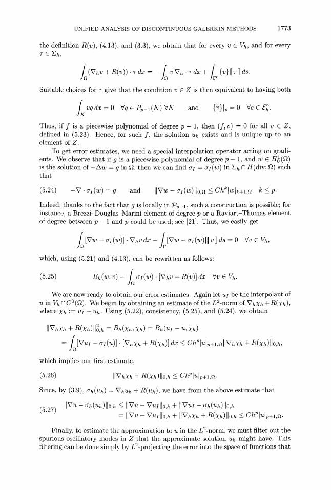
to the discrete problem, together with optimal rates of convergence, still can be ob- tained for suitable functions f. We proceed as follows. First, we find under what conditions on f an approximate solution uh exists. Integrating by parts and recalling
UNIFIED ANALYSIS OF DISCONTINUOUS GALERKIN METHODS 1773
the definition R(v), (4.13), and (3.3), we obtain that for every v E Vh, and for every TE h,
(VhV+ R(v))- Tdx= - jvVA .rT dx + j{v}ViTds.
Suitable choices for T give that the condition v E Z is then equivalent to having both
Svqdx= 0 Vq e
Pp-(K)VK
and {v}e -
0 Ve E eS.
Thus, if f is a piecewise polynomial of degree p - 1, then (f, v) = 0 for all v E Z, defined in (5.23). Hence, for such f, the solution Uh exists and is unique up to an element of Z.
To get error estimates, we need a special interpolation operator acting on gradi- ents. We observe that if g is a piecewise polynomial of degree p - 1, and w E H' (Q) is the solution of -Aw = g in Q, then we can find ac = ur(w) in Eh n H(div; Q) such that
(5.24) -V - I(w) = g and IlVw - ai(w)Ilo,Q < Chkwlk+l,Q k < p.
Indeed, thanks to the fact that g is locally in p,_1, such a construction is possible; for instance, a Brezzi-Douglas-Marini element of degree p or a Raviart-Thomas element of degree between p - 1 and p could be used; see [21]. Thus, we easily get
SVw -
OI(w)] Vhvdx - [Vw
-- I(w)][v•dsO 0
Vv E Vh,
which, using (5.21) and (4.13), can be rewritten as follows:
(5.25) Bh(w, v) = j u(w). [V hV+ R(v)] dx Vv E Vh
We are now ready to obtain our error estimates. Again let uz be the interpolant of u in Vh nCo(Qt).
We begin by obtaining an estimate of the L2-norm of VhXh + R(Xh), where Xh := uI - Uh. Using (5.22), consistency, (5.25), and (5.24), we obtain
(5.26) IlVhXh + R(xh) 10,h < ChPlulp+~,?. Since, by (3.9), ah(Uh) = VhUh + R(uh), we have from the above estimate that
I(5.27) Vu - ah(uh)llo,h I ilu - Vu lIO,h + IIVUI -- h(Uh)110,h = VIIu - Vull o,h + IVhXh + R(Xh)l O0,h ChPlulp+1,0.
Finally, to estimate the approximation to u in the L2-norm, we must filter out the spurious oscillatory modes in Z that the approximate solution uh might have. This filtering can be done simply by L2-projecting the error into the space of functions that
1774 D. N. ARNOLD, F. BREZZI, B. COCKBURN, AND L. D. MARINI
are piecewise polynomials of degree at most p - 1. In other words, if we denote by P,_1 such a projection, we simply estimate
Pp-1(u - uh) instead of u - Uh. We then
take 4 to be the solution of
-AO = P_-l(u
- Uh)
in Q, ,)
= 0 on oQ,
and 4', its continuous piecewise linear interpolant. Using adjoint consistency, then
(5.25) and (5.21), and finally (5.26) and interpolation estimates, we obtain
+llulp+l,a In other words, the L2-projection of the error into the space of piecewise polynomials of degree p - 1 superconverges.
6. Summary and concluding remarks. In this paper, we propose a general framework that allows us to obtain a unified analysis of virtually all the methods found in the literature for dealing with linear elliptic problems by means of DG methods.
We have shown that all these DG methods can be obtained by suitably choos-
ing the numerical fluxes in the flux formulation (1.2)-(1.3). We also made clear the connection between the flux and primal formulations and between consistency and conservativity of the numerical fluxes and consistency and adjoint consistency, respectively, of the primal formulation.
We found that DG methods that are completely consistent and stable achieve
optimal error estimates. Inconsistent DG methods, like the pure penalty methods, still can achieve optimal error estimates provided they are superpenalized. The same holds true for methods that lack adjoint consistency, such as the superpenalized version of the NIPG method.
The method of Baumann and Oden and its stabilized version, NIPG, are both consistent but, since they use nonconservative numerical fluxes i, they are not adjoint consistent. The lack of adjoint consistency of these two methods is reflected in a
suboptimal rate of convergence in the L2-norm. The stabilization of DG methods via the inclusion of a penalty term is crucial:
without it, convergence is degraded or lost. In terms of fluxes, stability is related to the suitable choice of the stabilizing term a in the vector flux. Fortunately, there are no apparent drawbacks to the inclusion of such terms. We considered here two forms of stabilization terms, one arising in the IP methods and the other in the method of Bassi et al. [13]. These are equivalent within a constant multiple as far as the analysis is concerned, although in some cases the condition on the coefficient r required for
stability can be made more explicit for the second form. A comparison of the relative
efficacy of the two approaches to stabilization remains to be made. Two methods without stabilizing terms were considered: the method of Baumann
and Oden and the original method of Bassi and Rebay. The former method is unstable for p = 1, but recovers what we have called weak stability for p > 2. In this case,
UNIFIED ANALYSIS OF DISCONTINUOUS GALERKIN METHODS 1775
TABLE 6.1 Properties of the DG methods.
Method Cons. A.C. Stab. Type Cond. H1 L2
Brezzi et al. [22] V/ / / ar ro > 0 hp hP+1
LDG [41] / / / j o70 > 0 hp hP+1
IP [50] / / / aj ro > r* hP hp+l1
Bassi et al. [13] / V/ / r 0O > 3 hp hp+l
NIPG [64] / x / aC r70 > 0 hp hp
Babulka-Zl~mal [7] x x V oj ra l 0 h-2p hp hp+1
Brezzi et al. [23] x x / or o70 h-2p hp hp+l
Baumann-Oden (p = 1) / x x - - x x
Baumann-Oden (p > 2) V/ x x - - hp hp
Bassi-Rebay [10] V V x - - [hP] [hp+1]
optimal error bounds can be proved in the H1-norm. The least stable method seems to be the first method of Bassi and Rebay, which might have a singular matrix on certain grids. However, the use of a right-hand side f which is locally a polynomial of degree p - 1 makes the system compatible, and then stability and optimal error bounds are achieved in a suitable seminorm (essentially obtained by projecting the error onto the space of piecewise polynomials of degree p - 1).
These results are summarized in Table 6.1, which reports, for the various meth-
ods, consistency, adjoint consistency, stability, type of stabilization term, theoretical
requirement on ro0 = infe ne for stability, and rates of convergence in H1(Th) and in L2. In the last row the brackets around the convergence rate are to remind us that the estimates (5.27) and (5.28) are bounds only on certain seminorms of the error.
Although we have considered only the model problem of the Laplacian with homo-
geneous Dirichlet boundary conditions on a convex polygon, extension of our frame- work and analysis to more general scalar elliptic operators and more general boundary conditions can be easily carried out. There can, however, be several variants of this extension since the definition of the auxiliary variable ah can take several forms; see, for example, [41] and [33]. Of course, DG methods also can be easily defined for nu-
merically approximating the solutions of more complex problems such as, for example, the system of linear elasticity, the Stokes system, the Maxwell equations, and plate problems. Much of the approach proposed in this paper can be carried over to those situations.
While the framework and analysis we have set out are helpful for comparing various DG methods and for comparing them with other methods, we certainly do not claim that they are sufficient for these purposes. We have mentioned in passing some
potential advantages of DG methods, especially their utility in convection-dominated
problems, the possibility of using nonconforming meshes, and perhaps their suitability for h-, p-, and hp-adaptivity. Moreover, a variety of other motivations for their use have been put forth by other authors in a variety of situations. Clearly, to ascertain the extent to which these advantages are realized for a particular DG method and a particular class of problems will require further work, especially numerical studies. A significant numerical comparison of DG methods for elliptic problems has been
1776 D. N. ARNOLD, F. BREZZI, B. COCKBURN, AND L. D. MARINI
recently carried out by Castillo [25]. In addition to questions of accuracy, he studied the condition number, the sparsity of the stiffness matrices, and the effect of varying the penalty parameter. In [12], Bassi and Rebay compared a few of the DG methods discussed here for the compressible Navier-Stokes equations.
There are two other directions for future research. One important issue is the
design of effective solvers for DG methods. Some results in this direction can be found already in Bassi and Rebay [11], Feng and Karakashian [51], Lasser and Toselli
[55], and Gopalakrishnan and Kanshat [53]. Finally, the coupling of DG methods with other methods seems attractive in some circumstances. See Alotto et al. [1] and
Perugia and Schotzau [60]. In view of the widespread and increasing interest in discontinuous Galerkin meth-
ods in recent years, we believe that such further studies are very worthwhile and hope that the framework presented here will prove useful.
REFERENCES
[1] P. ALOTTO. A. BERTONI, I. PERUGIA, AND D. SCH6TZAU, Discontinuous finite element methods
for the simulation of rotating electrical machines, COMPEL, 20 (2001), pp. 448-462.
[2] D. ARNOLD, F. BREZZI, B. COCKBURN, AND D. MARINI, Discontinuous Galerkin methods for elliptic problems, in Discontinuous Galerkin Methods. Theory, Computation and Applica- tions, B. Cockburn, G. E. Karniadakis, and C.-W. Shu, eds., Lecture Notes in Comput. Sci. Engrg. 11, Springer-Verlag, New York, 2000, pp. 89-101.
[3] D. N. ARNOLD, An Interior Penalty Finite Element Method with Discontinuous Elements, Ph.D. thesis, The University of Chicago, Chicago, IL, 1979.
[4] D. N. ARNOLD, An interior penalty finite element method with discontinuous elements, SIAM J. Numer. Anal., 19 (1982), pp. 742-760.
[5] J. P. AUBIN, Approximation des problkmes aux limites non homogenes pour des opdrateurs non lindaires, J. Math. Anal. Appl., 30 (1970), pp. 510-521.
[6] I. BABUSKA, The finite element method with penalty, Math. Comp., 27 (1973), pp. 221-228.
[7] I. BABUSKA AND MI. ZLA&MAL, Nonconforming elements in the finite element method with
penalty, SIAM J. Numer. Anal., 10 (1973), pp. 863-875.
[8] G. A. BAKER, Finite element methods for elliptic equations using nonconforming elements, Math. Comp., 31 (1977), pp. 45-59.
[9] G. A. BAKER, W. N. JUREIDINI, AND O. A. KARAKASHIAN, Piecewise solenoidal vector fields and the Stokes problem, SIAM J. Numer. Anal., 27 (1990), pp. 1466-1485.
[10] F. BASSI AND S. REBAY, A high-order accurate discontinuous finite element method for the
numerical solution of the compressible Navier-Stokes equations, J. Comput. Phys., 131
(1997), pp. 267-279. [11] F. BASSI AND S. REBAY, GMRES for discontinuous Galerkin solution of the compressible
Navier-Stokes equations, in Discontinuous Galerkin Methods. Theory, Computation and
Applications, B. Cockburn, G. E. Karniadakis, and C.-W. Shu, eds., Lecture Notes in
Comput. Sci. Engrg. 11, Springer-Verlag, New York, 2000, pp. 197-208.
[12] F. BASSI AND S. REBAY, Numerical evaluation of two discontinuous Galerkin methods for the
compressible Navier-Stokes equations, Internat. J. Numer. Methods Fluids, to appear. [13] F. BASSI, S. REBAY, G. MARIOTTI, S. PEDINOTTI, AND M. SAVINI, A high-order accurate
discontinuous finite element method for inviscid and viscous turbomachinery flows, in
Proceedings of 2nd European Conference on Turbomachinery, Fluid Dynamics and Ther-
modynamics, R. Decuypere and G. Dibelius, eds., Technologisch Instituut, Antwerpen, Belgium, 1997, pp. 99-108.
[14] C. E. BAUMANN AND J. T. ODEN, A Discontinuous hp finite element method for the Euler and Navier-Stokes equations, Internat. J. Numer. Methods Fluids, 31 (1999), pp. 79-95.
[15] C. E. BAUMANN AND J. T. ODEN, A discontinuous hp finite element method for convection- diffusion problems, Comput. Methods Appl. Mech. Engrg., 175 (1999), pp. 311-341.
[16] R. BECKER AND P. HANSBO, Discontinuous Galerkin methods for convection-diffusion problems with arbitrary Pdclet number, in Numerical Mathematics and Advanced Applications, Pro- ceedings of ENUMATH 99, P. Neittaanmilki, T. Tiihonen, and P. Tarvainen, eds., World Scientific, River Edge, NJ, 2000, pp. 100-109.
UNIFIED ANALYSIS OF DISCONTINUOUS GALERKIN METHODS 1777
[17] R. BECKER AND P. HANSBO, A Finite Element Method for Domain Decomposition with Non- Matching Grids, Tech. Report 3613, INRIA, Le Chesnay, France, 1999.
[18] C. BERNARDI, Y. MADAY, AND A. T. PATERA, Domain decomposition by the mortar element method, in Asymptotic and Numerical Methods for Partial Differential Equations with Critical Parameters, H. G. Kaper and M. Garbey, eds., Kluwer Academic Publishers, Dor- drecht, The Netherlands, 1993, pp. 269-286.
[19] C. BERNARDI, Y. MADAY, AND A. T. PATERA, A new nonconforming approach to domain decomposition: The mortar element method, in Nonlinear Partial Differential Equations and Their Applications, Collbge de France Seminar, Vol. XI, H. Brezis and J. L. Lions, eds., Pitman Res. Notes Math. Ser., 299, Longman Sci. Tech., Harlow, 1994, pp. 13-51.
[20] C. BERNARDI, N. DEBIT, AND Y. MADAY, Coupling finite element and spectral methods: First results, Math. Comp., 54 (1990), pp. 21-39.
[21] F. BREZZI AND M. FORTIN, Mixed and Hybrid Finite Element Methods, Springer-Verlag, New York, 1991.
[22] F. BREZZI, G. MANZINI, D. MARINI, P. PIETRA, AND A. Russo, Discontinuous finite elements
for diffusion problems, in Atti Convegno in onore di F. Brioschi (Milan, 1997), Istituto Lombardo, Accademia di Scienze e Lettere, Milan, Italy, 1999, pp. 197-217.
[23] F. BREZZI, G. MANZINI, D. MARINI, P. PIETRA, AND A. Russo, Discontinuous Galerkin approx- imations for elliptic problems, Numer. Methods Partial Differential Equations, 16 (2000), pp. 365-378.
[24] P. CASTILLO, An optimal error estimate for the local discontinuous Galerkin method, in Dis- continuous Galerkin Methods. Theory, Computation and Applications, B. Cockburn, G. E. Karniadakis, and C.-W. Shu, eds., Lecture Notes in Comput. Sci. Engrg., 11, Springer- Verlag, New York, 2000, pp. 285-290.
[25] P. CASTILLO, Performance of Discontinuous Galerkin Methods for Elliptic PDE's, IMA Preprint 1764, Minneapolis, MN, April 2001.
[26] P. CASTILLO, B. COCKBURN, I. PERUGIA, AND D. SCH6TZAU, An a priori error analysis of the local discontinuous Galerkin method for elliptic problems, SIAM J. Numer. Anal., 38 (2000), pp. 1676-1706.
[27] P. CASTILLO, B. COCKBURN, D. SCH6TZAU, AND C. SCHWAB, Optimal a priori error estimates for the hp-version of the local discontinuous Galerkin method for convection-diffusion prob- lems, Math. Comp., to appear.
[28] Z. CHEN, B. COCKBURN, C. GARDNER, AND J. JEROME, Quantum hydrodynamic simulation of hysteresis in the resonant tunneling diode, J. Comput. Phys., 117 (1995), pp. 274-280.
[29] Z. CHEN, B. COCKBURN, J. JEROME, AND C.-W. SHU, Mixed-RKDG finite element methods for the 2-D hydrodynamic model for semiconductor device simulation, VLSI Design, 3 (1995), pp. 145-158.
[30] P. CIARLET, The Finite Element Method for Elliptic Problems, North-Holland, Amsterdam, 1978.
[31] B. COCKBURN, Discontinuous Galerkin methods for convection-dominated problems, in High- Order Methods for Computational Physics, T. Barth and H. Deconink, eds., Lecture Notes in Comput. Sci. Engrg. 9, Springer-Verlag, New York, 1999, pp. 69-224.
[32] B. COCKBURN, Devising discontinuous Galerkin methods for non-linear hyperbolic conservation laws, J. Comput. Appl. Math., 128 (2001), pp. 187-204.
[33] B. COCKBURN AND C. DAWSON, Some extensions of the local discontinuous Galerkin method for convection-diffusion equations in multidimensions, in Proceedings of the Conference on the Mathematics of Finite Elements and Applications: MAFELAP X, J. R. Whiteman, ed., Elsevier, New York, 2000, pp. 225-238.
[34] B. COCKBURN, S. Hou, AND C.-W. SHU, TVB Runge-Kutta local projection discontinuous Galerkin finite element method for conservation laws IV: The multidimensional case, Math. Comp., 54 (1990), pp. 545-581.
[35] B. COCKBURN, J. JEROME, AND C.-W. SHU, The utility of modeling and simulation in determin- ing performance and symmetry properties of semiconductors, in Discontinuous Galerkin Methods. Theory, Computation and Applications, B. Cockburn, G. E. Karniadakis, and C.-W. Shu, eds., Lecture Notes in Comput. Sci. Engrg. 11, Springer-Verlag, New York, 2000, pp. 147-156.
[36] B. COCKBURN, G. KANSCHAT, I. PERUGIA, AND D. SCHOTZAU, Superconvergence of the local discontinuous Galerkin method for elliptic problems on Cartesian grids, SIAM J. Numer. Anal., 39 (2001), pp. 264-285.
1778 D. N. ARNOLD, F. BREZZI, B. COCKBURN, AND L. D. MARINI
[37] B. COCKBURN, G. E. KARNIADAKIS, AND C.-W. SHU, The development of discontinuous Galerkin methods, in Discontinuous Galerkin Methods. Theory, Computation and Appli- cations, B. Cockburn, G. E. Karniadakis, and C.-W. Shu, eds., Lecture Notes in Comput. Sci. Engrg. 11, Springer-Verlag, New York, 2000, pp. 3-50.
[38] B. COCKBURN, S. Y. LIN, AND C.-W. SHU, TVB Runge-Kutta local projection discontinuous Galerkin finite element method for conservation laws III: One dimensional systems, J. Comput. Phys., 84 (1989), pp. 90-113.
[39] B. COCKBURN AND C.-W. SHU, TVB Runge-Kutta local projection discontinuous Galerkin finite element method for scalar conservation laws II: General framework, Math. Comp., 52 (1989), pp. 411-435.
[40] B. COCKBURN AND C.-W. SHU, The Runge-Kutta local projection Pl-discontinuous Galerkin method for scalar conservation laws, RAIRO Model. Math. Anal. Numer., 25 (1991), pp. 337-361.
[41] B. COCKBURN AND C.-W. SHU, The local discontinuous Galerkin method for time-dependent convection-diffusion systems, SIAM J. Numer. Anal., 35 (1998), pp. 2440-2463.
[42] B. COCKBURN AND C.-W. SHU, The Runge-Kutta discontinuous Galerkin finite element method
for conservation laws V: Multidimensional systems, J. Comput. Phys., 141 (1998), pp. 199- 224.
[43] B. COCKBURN AND C.-W. SHU, Runge-Kutta discontinuous Galerkin methods for convection- dominated problems, J. Sci. Comput., to appear.
[44] C. N. DAWSON, Godunov-mixed methods for advection flow problems equations in one space dimension, SIAM J. Numer. Anal., 28 (1991), pp. 1282-1309.
[45] C. DAWSON, Godunov-mixed methods for advection-diffusion equations in multidimensions, SIAM J. Numer. Anal., 30 (1993), pp. 1315-1332.
[46] C. DAWSON, Analysis of an upwind-mixed finite element method for nonlinear contaminant transport equations, SIAM J. Numer. Anal., 35 (1998), pp. 1709-1724.
[47] C. N. DAWSON AND V. AIZINGER, Upwind-mixed methods for transport equations, Comp. Geosci., 3 (1999), pp. 93-110.
[48] E. G. DUTRA DO CARMO AND A. V. C. DUARTE, A discontinuous finite element-based domain decomposition method, Comput. Methods Appl. Mech. Engrg., 190 (2000), pp. 825-843.
[49] J. DOUGLAS. JR., B. L. DARLOW, R. P. KENDALL, AND M. F. WHEELER, Self-adaptive Galerkin methods for one-dimensional, two-phase immiscible flow, in Proceedings AIME Fifth Symposium on Reservoir Simulation (Denver, Colorado), Society of Petroleum Engi- neers, Dallas, TX, 1979, pp. 65-72.
[50] J. DOUGLAS, JR. AND T. DUPONT, Interior Penalty Procedures for Elliptic and Parabolic Galerkin Methods, Lecture Notes in Phys. 58, Springer-Verlag, Berlin, 1976.
[51] X. FENG AND O. A. KARAKASHIAN, Two-level additive Schwarz methods for a discontinu- ous Galerkin approximation of second order elliptic problems, SIAM J. Numer. Anal., 39
(2001), pp. 1343-1365. [52] J. GREENSTADT, An abridged history of cell discretization, in Discontinuous Galerkin Methods.
Theory, Computation and Applications, B. Cockburn, G. E. Karniadakis, and C.-W. Shu, eds., Lecture Notes in Comput. Sci. Engrg. 11, Springer-Verlag, New York, 2000, pp. 337- 342.
[53] J. GOPALAKRISHNAN AND G. KANSHAT, A multilevel discontinuous Galerkin method, Numer. Math., to appear.
[54] P. HOUSTON, C. SCHWAB, AND E. SiULI, Discontinuous hp Finite Element Methods for Advection-Diffusion Problems, Tech. Report NA 00-15, Oxford University Computing Lab-
oratory, Oxford, UK, 2000. [55] C. LASSER AND A. TOSELLI, An Overlapping Domain Decomposition Preconditioner for a Class
of Discontinuous Galerkin Approximations of Advection-Diffusion Problems, Tech. Report 2000-12, Seminar fiir Angewandte Mathematik, ETH Ziirich, 2000.
[56] J.-L. LIONS, Problkmes aux limites non homogknes a donees irrigulikres: Une mithode d'approximation, in Numerical Analysis of Partial Differential Equations (C.I.M.E. 2 Ciclo, Ispra, 1967), Edizioni Cremonese, Rome, 1968, pp. 283-292.
[57] I. LOMTEV, C. W. QUILLEN,
AND G. E. KARNIADAKIS, Spectral/hp methods for viscous com- pressible flows on unstructured 2D meshes, J. Comput. Phys., 144 (1998), pp. 325-357.
[58] J. A. NITSCHE, Uber ein Variationsprinzip zur Losung Dirichlet-Problemen bei Verwendung von Teilriiumen, die keinen Randbedingungen unteworfen sind, Abh. Math. Sem. Univ. Hamburg, 36 (1971), pp. 9-15.
[59] J. T. ODEN, IVO BABUSKA, AND C. E. BAUMANN, A discontinuous hp finite element method
for diffusion problems, J. Comput. Phys., 146 (1998), pp. 491-519.
UNIFIED ANALYSIS OF DISCONTINUOUS GALERKIN METHODS 1779
[60] I. PERUGIA AND D. SCH6TZAU, On the coupling of local discontinuous Galerkin and conforming finite element methods, J. Sci. Comput., to appear.
[61] W. H. REED AND T. R. HILL, Triangular Mesh Methods for the Neutron Transport Equation, Tech. Report LA-UR-73-479, Los Alamos Scientific Laboratory, Los Alamos, NM, 1973.
[62] G. R. RICHTER, The discontinuous Galerkin method with diffusion, Math. Comp., 58 (1992), pp. 631-643.
[63] B. RIVIERE AND M. F. WHEELER, A discontinuous Galerkin method applied to nonlinear
parabolic equations, in Discontinuous Galerkin Methods. Theory, Computation and Appli- cations, B. Cockburn, G. E. Karniadakis, and C.-W. Shu, eds., Lecture Notes in Comput. Sci. Engrg. 11, Springer-Verlag, New York, 2000, pp. 231-244.
[64] B. RIVIIRE, M. F. WHEELER, AND V. GIRAULT, Improved energy estimates for interior penalty, constrained and discontinuous Galerkin methods for elliptic problems I, Comput. Geosci., 3 (1999), pp. 337-360.
[65] T. RUSTEN, P. S. VASSILEVSKI, AND R. WINTHER, Interior penalty preconditioners for mixed finite element approximations of elliptic problems, Math. Comp., 65 (1996), pp. 447-466.
[66] C.-W. SHU, Different formulations of the discontinuous Galerkin method for the viscous terms, in Proceedings of Conference in Honor of Professor H.-C. Huang on the Occasion of His
Retirement, W. M. Xue, Z. C. Shi, M. Mu, and J. Zou, eds., Science Press, New York, Beijing, 2000, pp. 14-45.
[67] E. SULI, P. HOUSTON, AND C. SCHWAB, hp-finite element methods for hyperbolic problems, in
Proceedings of the Conference on the Mathematics of Finite Elements and Applications: MAFELAP X, J. R. Whiteman, ed., Elsevier, New York, 2000, pp. 143-162.
[68] E. SiLI, C. SCHWAB, AND P. HOUSTON, hp-DGFEM for partial differential equations with non-
negative characteristic form, in Discontinuous Galerkin Methods. Theory, Computation and Applications, B. Cockburn, G. E. Karniadakis, and C.-W. Shu, eds., Lecture Notes in
Comput. Sci. Engrg. 11, Springer-Verlag, New York, 2000, pp. 221-230.
[69] H. SWANN, The cell discretization algorithm: An overview, in Discontinuous Galerkin Methods.
Theory, Computation and Applications, B. Cockburn, G. E. Karniadakis, and C.-W. Shu, eds., Lecture Notes in Comput. Sci. Engrg. 11, Springer-Verlag, New York, 2000, pp. 433- 438.
[70] M. F. WHEELER, An elliptic collocation-finite element method with interior penalties, SIAM J. Numer. Anal., 15 (1978), pp. 152-161.