ATHESIS

SUBMITTED IN PARTIAL FULFILLMENT OF THE REQUIREMENTSFOR THE HONORS DEGREE OF

BACHELOR OF SCIENCE IN PHYSICS

Unifying Inflation and Dark Energy Using an Interacting Holographic ModelAbby E. Besemer

DEPARTMENT OF PHYSICSINDIANA UNIVERSITY

April 28, 2010

Supervisor:Michael Berger

Co-signer:Richard Van Kooten

1

Unifying Inflation and Dark Energy Using an Interacting

Holographic Model

Abby Besemer∗

Advisor: Michael Berger†

Physics Department, Indiana UniversityPhysics and Astronomy Senior Honors Thesis

April 28, 2010

Abstract

The universe has gone through at least two very different periods of accelerated expansion.The earliest stage was a rapid exponential expansion known as inflation while the accelerationwe are experiencing at the current epoch is driven by dark energy. Because the energy scale ofdark energy is many orders of magnitude smaller than that of inflation, the relationship betweenthe two periods of acceleration is unknown. The introduction of an interaction between darkenergy and matter and the holographic principle offers a possible way to unify these two erasof expansion using a model based on a simple physical principle. Here we present a possibleexpansion history for the universe using a model of interacting holographic dark energy.

∗abesemer@indiana.edu†berger@indiana.edu

2

Introduction

The theorized exponential expansion of the early Universe called Inflation is considered part ofthe standard big bang cosmology. It was proposed to smooth out any inhomogeneities, anisotropiesand curvature in the Universe. Until the late 1990’s it was believed that matter’s gravitationalattraction has since been slowing down the expansion. Then in 1998, the HST observed the redshift-distance relation of Type Ia supernovae and revealed that the Universe has actually begun toaccelerate again [1]. It is believed that this acceleration is driven by a mysterious cosmologicalcomponent called dark energy. The matter energy density naturally decreases as the Universeexpands and at some point in the not so distant past, dark energy began to dominate the totalenergy density of the Universe and thereby initiated the second accelerated expansion.

Models of interacting dark energy have been employed in the past to offer a possible solution tothe cosmic coincidence problem of why the matter (Ωm ≈ .3) and dark energy (ΩΛ ≈ .7) densitiesare so close at the present epoch [2, 3]. In these models there exists a mechanism that converts darkenergy to matter so that the energy densities become comparable at late times, thus solving thecosmic coincidence problem. For our purposes, an interaction provides a way to unite the expansionhistory of the Universe using a simple physical principle. Even though we do not specify the physicalmechanism for the interaction, it provides an interesting way to explain the observed cosmologicalquantities at a phenomenological level [2]. The nature of such an interaction is something that canbe investigated once the nature of dark energy itself is better known.

This model also uses a holographic principle in order to account for the small scale of the darkenergy density (ρ0 ≈ 3× 10−3eV 4 where the subscript “0” indicates the value at the present time)[4]. This principle is motivated by the fact that the present value for the dark energy density seemsto be consistant with taking the geometric average with the Planck mass Mpl and the size of theUniverse given by the Hubble parameter H0 [4, 2]. Essentially, imposing holography on dark energyallows the density to be expressed in terms of some length scale associated with a horizon.

The cosmology of interacting dark energy is described by the Freidmann equations. The equilib-rium points of these equations determine how the Universe evolves. This paper presents a possibleexpansion history assuming that the Universe consists of dark energy, matter, negligible radiation,and non-zero curvature. We know that currently the Universe is flat within a margin of 2% [5], butthis may not have always been so. Without curvature, the equilibria of the Friedmann equationsdescribe a fixed point that the Universe will either evolve away from (repelling fixed point) ortowards (attracting fixed point). By allowing curvature to evolve similar to the other cosmologicalcomponents, it is possible for these equilibria to become saddle points representing a transitionalstate which is the key to tying inflation in to the rest of the expansion history. Here we show thatan interaction and holographic condition for dark energy allows the Universe to start out in a darkenergy dominated state, experience a transitional period of inflation and matter creation, and thenevolve towards zero curvature where the dark energy density begins to take over again causing asecond period of acceleration.

Evolution Equations

The relative expansion of the Universe can be described by a scale factor a(t) which relatesthe comoving distance lt at time t to the distance lp is at the present time tp through the relationa(t) = lt/lp. The evolution of the scale factor can be determined from Friedmann equations for a

3

Friedmann-Lemaıtre-Robertson-Walker (FLRW) Universe:

H2 ≡(a

a

)2

=8πG

3ρ− k

a2, (1)

H =a

a= −4πG

3(1 + 3ω) ρ,

where H is the Hubble parameter and ω is the native equation of state that descibes the ratio ofthe pressure and density P/ρ. k is a contstant that defines the spatial curvature and k equals 1,-1, and 0 for a closed, open, and flat Universe respectively [6]. Here the constants c and h havebeen defined as 1 and the dot refers to the time deriviative. The pair of equations in (1) lead tothe following continuity equations for dark energy and matter:

ρΛ + 3H(1 + ωΛ)ρΛ = 0,ρm + 3H(1 + ωm)ρm = 0. (2)

In the presence of an interaction that converts the dark energy into matter, an interaction term Qappears on the right hand side of the continuity equations in order to ensure the conservation ofthe energy momentum tensor so that

ρΛ + 3H(1 + ωΛ)ρΛ = −Q,ρm + 3H(1 + ωm)ρm = Q. (3)

However, the interaction can be combined with the native equations of state in order to make acomparison with the ΛCDM model easier [4]. The effective equations of state can then be definedas

ωeffΛ = ωΛ +

Γ3H

and ωeffm = −1

r

Γ3H

. (4)

Here the rate Γ = Q/ρΛ and the ratio r = ρm/ρΛ have been defined for simplification. Additionally,one usually takes ωm = 0 assuming matter is pressureless. The continuity equations then become

ρΛ + 3H(1 + ωeffΛ )ρΛ = 0, (5)

ρm + 3H(1 + ωeffm )ρm = 0.

When the equations are written in this way it is easier to see that when there is no interaction,Q = 0, then the right-hand side of the differential equations is zero and the effective equations ofstate reduce to the native ones.

It is often more convenient to refer to the energy densities in terms of the energy densityparameter Ωi which is the ratio of the energy density and the critical energy density required tohave a flat universe Ωi ≡ ρi/ρcritical. The energy density parameter for each component is thengiven by

ΩΛ =8πρΛ

3M2plH

2, Ωm =

8πρm

3M2plH

2, Ωk =

k

a2H2. (6)

These are defined in this way so that the Friedmann equation in Eq (1) gives the relation

Ωm + ΩΛ = 1 + Ωk. (7)

4

The Ωk term can be thought of as the energy density parameter of curvature [6]. Even thoughit does not represent a real energy density, it “contributes to the expansion rate analogously tothe honest density parameters” [6]. Using these definitions, we can then rewrite the continuityequations in a more suggestive form using the energy density parameters. The ratio r and its timederivative can then be written in terms of the density parameters

r ≡ ρm

ρΛ=

1 + Ωk − ΩΛ

ΩΛand r ≡ 3H

(ωΛ − ωm +

1 + r

r

Γ3H

)= 3Hr(ωeff

Λ − ωeffm ). (8)

From these, we can then write the differential equations describing the time evolution of the densityparameters as

dΩΛ

dx= −3ΩΛ(1− ΩΛ)(ωeff

Λ − ωeffm ) + ΩΛΩk(1 + 3ωeff

m ),

dΩk

dx= 3ΩkΩΛ(ωeff

Λ − ωeffm ) + Ωk(1 + Ωk)(1 + 3ωeff

m ), (9)

dΩm

dx= 3ΩmΩΛ(ωeff

Λ − ωeffm ) + ΩmΩk(1 + 3ωeff

m ),

where Ωi = H ∂Ωi∂x and x = ln(a/a0). However, because of the relation in Eq. (7), the third

differential equation is redundant.Then by combining the Friedmann equations (1) and the evolution equations (9) for the density

parameters we can derive the evolution of the Hubble parameter

1H

dH

dx=

H

H2= −3

2(1 + ωΛΩΛ)− 1

2Ωk. (10)

Physical Assumptions

In order to determine the evolution of the density parameters, two physical assumptions arerequired [4]. One specification that can be made is a choice of an interaction Γ which involvesdefining how the ratio of rates Γ/H depends on Ωm, Ωk, and ΩΛ. The second specification is anassumption about the native equations of state of dark energy ωΛ. Lastly, an assumption aboutthe holographic principle for dark energy can be made. This is commonly done by specifying thedark energy density ρΛ in terms of a length scale LΛ through

ρΛ =3c2M2

pl

8πLΛ2 . (11)

Common choices for length scales include the Hubble horizon, Particle horizon, and Future horizon.In the ΛCDM model, a cosmological constant implies that the dark energy density is constant withtime and therefore requires that LΛ/LΛ = 0. The assumptions of an interaction, native equationof state, and holographic principle are not independent [4], but are related through the expression

Γ3H

= (−1− ωΛ) +2

3HLΛ

LΛ. (12)

Therefore, the specification of two physical assumptions determines the third.

5

The evolution of the Hubble parameter can then be rewritten as a function of the above terms

1H

dH

dx=

H

H2= −3

2(1− ΩΛ)− ΩΛ

H

LΛ

LΛ+

Γ2H

ΩΛ. (13)

Equilibria Solutions

The equilibrium points of the energy density evolution equations, Eqs. (9), occur when theright-hand sides are zero. The first kind of equilibria is a fixed point in (ΩΛ, Ωk) space. By settingthe differential equations in Eqs. (9) equal to zero and solving the linear combination, it can be seenthat these fixed points occur at (ΩΛ, Ωk) = (0,0), (1,0), (0,-1) unless the effective equations of state,Eqs (4) are defined in such a way that they have singularities at these points. The second kind ofequilibrium occurs when one density parameter is specified and a constraint is put on the effectiveequation of state. The existance of these points depend strongly on the two physical assumptions(holographic principle, interaction, or native equation of state) made, but one can see that thesemay occur when ΩΛ = 0 and ωeff

m = −1/3 or when Ωk = 0 and ωeffm = ωeff

Λ . Lastly, a constrainton just the effective equations of state can be made and it can be seen that the right-hand side ofthe evolution equations are zero when ωeff

m = ωeffΛ = −1/3.

Without curvature, these equilibria describe a fixed point that the Universe will either evolveaway from (repelling fixed point) or towards (attracting fixed point). By allowing curvature toevolve similar to the other the cosmological components as the Universe expands, it is possible forthese equilibria to become saddle points representing a transitional state. The behavior near thesepoints is important because it does not depend on the choice of initial conditions. The nature ofthese fixed points can be determined from the eigenvalues of the Jacobian matrix A composed ofthe first order partial derivitives of the evolution Eqs. (9) [7, 8, 9]. If the evolution equations aregenerally given by

dΩdx

= f(ΩΛ,Ωk), (14)

then the eigenvalues can be determined from the 2-by-2 matrix

A =

(∂f1

∂ΩΛ

∂f2

∂ΩΛ∂f1

∂Ωk

∂f2

∂Ωk

). (15)

If the resulting eigenvalues are both negative at a certain fixed point, then that equilibria point isan attractor and the Universe will eventually evolve towards this state. If both of the eigenvaluesare positive, then this equilibria point will be a repeller and the Universe will evolve away from thispoint. Lastly, if one eigenvalue is positive and one is negative then the fixed point will be a saddlepoint representing a transitional period.

In the case of no interaction Γ = 0 and constant dark energy L/L = 0 one retains the familiarbehavior of the ΛCDM model where the Universe is driven from a small amount of vacuum energyΩΛ ≈ 0 towards a de Sitter Universe at the attractive fixed point at (1,0) [4].

Possible Expansion Histories

We have found an interesting expansion history that exhibits an evolution that is bound to thetriangular region where ΩΛ and Ωm are always positive and vary between 0 and 1 and where Ωk is

6

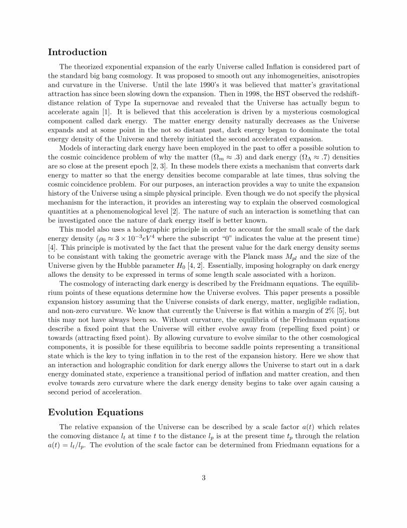
always negative and varies between -1 and 0. This solution can be seen in Figure 1. Because of therelation between the density parameters, Eq. (7), the line 1 + Ωk−ΩΛ = 0 corresponds to Ωm = 0.This line can be thought of as the matter axis and since the density of matter is physically requiredto be greater than zero, the Universe must evolve in the shaded region above this line. The originthen corresponds to when Ωm = 1.

Figure 1: A vector flow diagram of the evolution of the density parameters

As previously mentioned, the behavior of the density parameters requires the specification oftwo physical assumptions. In order to obtain this triangular region in the vector field, certainconstraints must be put on our choices for the physical assumptions. There are two requirementsin order to have the vertical flow lines on the ΩΛ = 0 line point in the positive direction. Firstly,in order to have

∂Ωk

∂x> 0 (16)

on the ΩΛ = 0 line, the differential equation for Ωk requires that

ωΛ ∝1

ΩΛ. (17)

Additionally, in order to have∂ΩΛ

∂x∝ ΩΛ (18)

on the ΩΛ = 0 line, the differential equation for ΩΛ requires that

Γ3H∝ 1

ΩΛ. (19)

The other constraint on the interaction comes from the requirement that

∂Ωm

∂x∝ Ωm (20)

on the Ωm = 0 line. This then requiresΓ

3H∝ Ωm. (21)

For the evolution seen in Figure 1, the interaction was chosen to be

Γ3H

=(1 + Ωk − ΩΛ)(1− ciΩΛ)

2ΩΛ(22)

7

where ci = 0.4, and the equation of state of dark energy was chosen to be

ωΛ =− (1 + ΩΛ)

(1 + Ωk − Ωk

2(

5ΩΛ1−ΩΛ

)− ΩΛ

)2ΩΛ(1− ΩΛ)

(23)

and the lengthscale was chosen such that

23H

LΛ

LΛ=

3(2(ΩΛ − 1)3 + 25Ωk2(1 + ΩΛ)− 2Ωk(6− 7ΩΛ + ΩΛ

2))20(ΩΛ − 1)2

. (24)

This solution has two saddle points at (ΩΛ,Ωk) = (0, 0) and (0,−1). Additionally, the regionnear (1, 0) exhibits saddle like behavior even though the differential equations are undefined at thispoint. Now, we assume that the Universe should start out in a dark energy dominated state withlittle or no matter, which corresponds to the region near (1, 0). Additionally, observational datasuggests that we currently live in a period where the total energy density is composed of about70% dark energy and about 30% matter and the curvature is almost perfectly flat [5]. Therefore,this requires the initial conditions be chosen such that the Universe will evolve through these tworegions such as the ones chosen in Figure 1. The blue line then represents the evolution of the thedensity parameters given those particular initial conditions.

(a) (b)

Figure 2: (a) The blue line represents the evolution of the the density parameters given initial conditions

of (ΩΛ, Ωk) = (0.8,−1.1 × 10−5). With these initial conditions, the evolution passes through a period where

(ΩΛ, Ωk, Ωm) ≈ (.7, 0, .3) which agrees with the observational data for the present day values for the density pa-

rameters. (b) The evolution of the density parameters as a function for x, where x = ln(a/a0).

In Figure 2, the Universe starts out in a dark energy dominated state with little or no matter.Then, because the interaction, Eq. (22), is proportional to the amount of matter, the interaction willremain weak and the Universe will evolve along the diagonal Ωm = 0 line. As the dark energy densitydecreases, the interaction gets stronger and begins creating matter while the curvature is driventowards zero. Then as the Universe evolves along the Ωk = 0 line from (0, 0) towards (1, 0), theinteraction gets weaker and the matter density then begins to decrease as the Universe expands, likeit would naturally in the absence of an interaction. Dark energy will then begin to dominate the totalenergy density as the Universe approaches the point (1, 0) and it will pass through a period whereΩm ≈ 0.274, ΩΛ ≈ 0.724, and Ωk ≈ −0.0011. These values for the density parameters are all withinthe uncertainty of the values that we observe today where Ωm = 0.281+0.016

−0.015, and ΩΛ = 0.724+0.015−0.016,

8

and Ωk = 0.0046+0.0068−0.0067 [5]. Then, in this particular solution, there is an additional attracting fixed

point in the interior of the triangle. This will cause the Universe to spiral towards this point wherethe density parameters will become nearly constant.

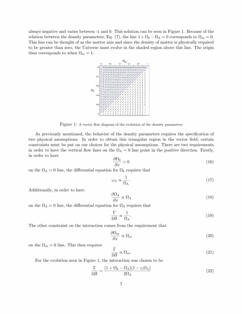
Four different types of interior points can occur within the triangle by making slightly differentchoices for the physical assumptions. This interior fixed point corresponds to when the effectiveequations of state for matter and dark energy are equal, ωeff

Λ = ωeffm = −1/3. If both the

eigenvalues are positive at this point, the interior point will be a repeller and the Universe will keepcirculating around the triangle edges of the triangle and will evolve closer and closer to the densityparameter axes with each evolution. If both the eigenvalues are negative, then the interior pointwill be an attractor and the Universe spiral towards this point regardless of the initial conditionschosen. An example of an attracting equilibrium point can be seen in Figure 3 (a). If the interiorpoint has two zero eigenvalues then it is neither an attractor or a repeller. In this case, the Universeevolves along cyclic paths and the behavior seems to suggest the conservation of some unknownquantity. An example of this type of solution can be see in Figure 3 (b). Lastly, if there aren’tany interior equilibrium points, then the solution will only evolve around the triangle once and willcontinue to approach the point (ΩΛ,Ωk) = (1, 0) where dark energy dominates the total energydensity of the Universe. An example of this type of solution can be see in Figure 3 (c). Whetherany of these evolutions would be more desirable than the others is still unclear. However, thesimplicity of an interior fixed point with zero eigenvalues makes it a slightly more attractive result.Also, an interior repelling point would allow the Universe to go through multiple increasing periodsof inflation.

(a) (b) (c)

Figure 3: The behavior of various expansion histories is determined by the existence of an additional equilibrium

point corresponding to when ωeffΛ = ωeff

m = −1/3. (a) This solution has an interior attracting fixed point which

causes the Universe to spiral towards this point. (b) This solution has an interior fixed point that is neither attracting

or repelling causing a cyclic evolution. (c) This solution does not have an interior fixed point and will only evolve

around the triangle once.

We have shown that an interacting holographic model is able to produce an expansion historythat passes through a period where the matter, dark energy, and curvature parameters are veryclose to the values that we observe today. But in order to see if this model can unify the acceleratedexpansions caused by dark energy and inflation, we have to look at the evolution of the Hubbleparameter. During the inflation phase, the Universe was dominated by some sort of scalar fieldthat had a large energy density that varied slowly with time. The Friedmann equations thenrequire the Hubble parameter H to be nearly constant during inflation as the Universe expanded

9

like a(t) = eHt. The differential equations describing the evolution of the Hubble parameter canbe seen in Eq. (10). Now, since the initial conditions require the Universe to start near the upperright-hand corner we can design the universe to inflate at the point (1, 0). Near that point, theright hand side of Eq. (13) reduces to −3/2(1 +ωΛ). Therefore, if ωΛ = −1 at this point, the righthand side of Eq. (13) will be zero, H will be constant, and the universe will inflate as long as itpasses close enough to this point.

During inflation the universe must expand by a factor of about 60 e-foldings, or a(t2)/a(t1) ≈e60, in order to smooth out any inhomogeneities and anisotropies in the cosmic microwave back-ground [12]. Therefore, because x = ln(a/a0), H is required to be constant for at least x = 60 inorder to have an inflation of 60 e-foldings. In order to see how the solution is behaving near thepoint (1,0) we can use perturbation theory and set ΩΛ = 1 − εΛ and Ωk = εk. The differentialequations that describe the behavior of εΛ and εk are given by

∂εΛ∂x

= −aεΛ + (higher order terms)

∂εk∂x

= −bεk −εk

2

εΛ+ (higher order terms). (25)

Therefore, to the first order, εΛ and εk can be approximated by

εΛ = εΛ,0e−ax (26)

εk = εk,0e−bx (27)

where the coefficients a and b determine how rapidly the Universe is approaching the point (1,0).From Eqs. 25 we can see that the Universe will start to turn around and leave the point (1,0) whenthe second order term εk

2/εΛ becomes comparable to bεk. This happens when

xt =1

a− bln

(εk,0

εΛ,0

)(28)

where xt denotes the value x when the turnaround occurs. From this equation, we can see thatthere are four ways to control the amount of time that the Universe stays near (1,0) and hencecontrol the amount of inflation. One way to increase the amount of inflation is to increase the powerof εΛ,0 and/or decrease the power of εk,0. However, the physical assumptions that must be chosento make these adjustments make it difficult to retain the triangular behavior in the vector fielddiagram. Another way to increase the amount of inflation is to make the values of the coefficientsa and b close to one another. It turns out that the values of a can be made arbitrarily close to b bysimply adjusting the coefficient ci in the interaction in Eq. (22). The coefficient ci also happens todetermine the nature of the point in the interior of the triangle. When ci ≤ 1/3 the interior fixedpoint disappears and the Universe will then be attracted to the point (1,0) and will not turn aroundjust as in Figure 3 (c). However, as long as ci > 1/3, for these choices of physics assumptions,there will be an interior fixed point and the Universe will pass near (1,0) without being attractedto it. Additionally, the closer ci gets to 1/3, the closer the values of a and b become and the moreattractive the point (1,0) becomes. The evolution of the Hubble parameter, H, as a function ofx for various choices of ci can be seen in Figure 4 (a). As expected, the closer ci gets to 1/3 thelonger the Universe will inflate. The last way to control the amount of inflation is to adjust theinitial conditions. The smaller value we choose for Ωk,0, the closer it will start to the edge of the

10

(a) (b)

Figure 4: The evolution of the Hubble parameter for various choices of (a) interaction coefficients ci and (c) initial

conditions. The red curve in both plots have a region where ln(H) is nearly constant for x = 60 corresponding to an

inflation of about 60 e-foldings.

triangle and the longer it will stick around the point (1,0). Figure 4 (b) shows the evolution of theHubble parameter for various choices of Ωk,0. As expected, smaller values Ωk,0 cause the Universeto inflate longer. The red curve in both Figure 4 (a) and (b) represents the desired inflation of atleast 60 e-foldings.

In order to determine what time corresponds to the various phases of the evolution, we can solvefor the time elapsed, te = tf/ti, as a function of x. This can be calculated by using the definitionof the Hubble parameter where

H(x) =a

a=

d

dtln(a) =

dx

dt(29)

and then integrating the Hubble parameter with respect to x∫ tf

ti

dt =∫ xf

xi

1H(x)

dx

te =∫ xf

xi

1H(x)

dx. (30)

For the evolution seen in Figure 2, the time elapsed, te = tf/ti, is plotted as a function ofx in Figure 5. Because our equations may not be valid before the Planck time, we will assumethat the evolution must start after this time and assume that ti = tpl ≈ 10−43s. The light blueregion in Figure 5 corresponds to the period of time when the Universe is near (ΩΛ,Ωk) = (1, 0)and inflating. This happens very rapidly and lasts until about 6.9 × 10−42s. The purple regionrepresents the period of time when the Universe starts to turn away from the point (1,0) but isnot inflating. Most of the time elapses during this part of the expansion history and lasts untilabout 60 yrs after the big bang. The red region represents when Ωm = 0 and this period lasts untilabout 2 × 104 yrs. Then the yellow region corresponds to when the interaction starts to becomestronger and the curvature is driven back up towards zero along the ΩΛ = 0 line. The Universethen reaches the origin at about 5.2× 108 yrs. Finally, the green region represents the time whenΩk = 0. The dark energy density starts to dominate the total energy density as the Universe moves

11

(a) (b)

Figure 5: The time elapsed, te = tf/ti, as a function of x. The light blue corresponds to inflation, the purple

corresponds to when the Universe is very near to the point (1,0) but not inflating, the red corresponds to when

Ωm = 0, the yellow corresponds to when ΩΛ = 0, the green corresponds to when Ωk = 0 until it reaches the dotted

line which represents the present day values for the density parameters.

along this line. The dotted line then corresponds to the time when the density parameters becomecomparable to the present day values. This occurs at an age of 12 × 109 yrs which is slightly lessthan 13.75± 0.17× 109 yrs, the current age of the Universe [13].

However, at the expense of fine-tuning, we can easily increase the lifetime to be exactly the ageof the universe at the point where Ωm ≈ 0.274, ΩΛ ≈ 0.724, and Ωk ≈ −0.0011 by simply adjustingthe coefficient, ce, in the equation of state

ωΛ =− (1 + ΩΛ)

(1 + Ωk − Ωk

2(

ceΩΛ1−ΩΛ

)− ΩΛ

)2ΩΛ(1− ΩΛ)

. (31)

In the case that ce = 0, ωΛ would be proportional to 1 + Ωk − ΩΛ or Ωm. Then, as the Universetravels along the Ωk = 0 line, Ωk ≈ 0 and ωΛ simplifies to

ωΛ ≈ − (1 + ΩΛ) (1− ΩΛ)2ΩΛ(1− ΩΛ)

≈ − (1 + ΩΛ)2ΩΛ

. (32)

Then as ΩΛ → 1, we have ωΛ → −1 and the Universe will inflate near (1,0). However, whenthe Universe starts to turn away from this point, Ωk starts to increase and the Ωm term stopscancelling with the (1 − ΩΛ) term and ωΛ can no longer be approximated as -1 which is requiredto have inflation. In the case that ce = 0, ωΛ will start to deviate from -1 and stop inflatingeven though it remains close to the point (1,0). Because of this, a lot of time is spent near thispoint and causes the whole evolution to last longer then the age of the Universe. The addition ofthe Ωk

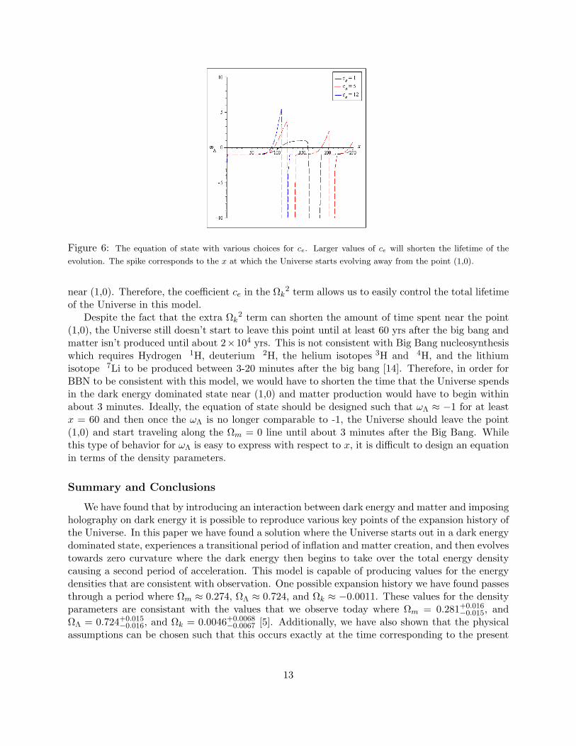
2 term changes the way the numerator cancels with the denominator near the point (1,0)and, consequently, larger values of ce will decrease the amount of time spent near (1,0) while notinflating. Plots of the equation of state with various choices for ce can be seen in Figure 6. Largervalues of ce will shorten the entire lifetime of the evolution, by decreasing the amount of time spent

12

Figure 6: The equation of state with various choices for ce. Larger values of ce will shorten the lifetime of the

evolution. The spike corresponds to the x at which the Universe starts evolving away from the point (1,0).

near (1,0). Therefore, the coefficient ce in the Ωk2 term allows us to easily control the total lifetime

of the Universe in this model.Despite the fact that the extra Ωk

2 term can shorten the amount of time spent near the point(1,0), the Universe still doesn’t start to leave this point until at least 60 yrs after the big bang andmatter isn’t produced until about 2×104 yrs. This is not consistent with Big Bang nucleosynthesiswhich requires Hydrogen 1H, deuterium 2H, the helium isotopes 3H and 4H, and the lithiumisotope 7Li to be produced between 3-20 minutes after the big bang [14]. Therefore, in order forBBN to be consistent with this model, we would have to shorten the time that the Universe spendsin the dark energy dominated state near (1,0) and matter production would have to begin withinabout 3 minutes. Ideally, the equation of state should be designed such that ωΛ ≈ −1 for at leastx = 60 and then once the ωΛ is no longer comparable to -1, the Universe should leave the point(1,0) and start traveling along the Ωm = 0 line until about 3 minutes after the Big Bang. Whilethis type of behavior for ωΛ is easy to express with respect to x, it is difficult to design an equationin terms of the density parameters.

Summary and Conclusions

We have found that by introducing an interaction between dark energy and matter and imposingholography on dark energy it is possible to reproduce various key points of the expansion history ofthe Universe. In this paper we have found a solution where the Universe starts out in a dark energydominated state, experiences a transitional period of inflation and matter creation, and then evolvestowards zero curvature where the dark energy then begins to take over the total energy densitycausing a second period of acceleration. This model is capable of producing values for the energydensities that are consistent with observation. One possible expansion history we have found passesthrough a period where Ωm ≈ 0.274, ΩΛ ≈ 0.724, and Ωk ≈ −0.0011. These values for the densityparameters are consistant with the values that we observe today where Ωm = 0.281+0.016

−0.015, andΩΛ = 0.724+0.015

−0.016, and Ωk = 0.0046+0.0068−0.0067 [5]. Additionally, we have also shown that the physical

assumptions can be chosen such that this occurs exactly at the time corresponding to the present

13

day age of the Universe.In this paper we have also found that an interacting holographic model is also capable of unifying

the accelerated expansions caused by dark energy and inflation as long as the initial conditions arechosen such that the solution passes through the region where the Hubble parameter is nearlyconstant. The interaction can then be chosen such that the Hubble parameter will remain constantfor a period of at least x = 60 and the Universe will inflate by a factor of about 60 e-foldings,or a(t2)/a(t1) ≈ e60, which is required to smooth out any inhomogeneities and anisotropies in thecosmic microwave background [12].

To further improve this model and to be consistent with Big Bang nucleosynthesis, the equationof state, ωΛ, needs to be chosen such that inflation, as well as the start of matter production, willoccur within the first 3 minutes of the Universe. Additionally, in order to eliminate some ofthe fine-tuning in this model, we ultimately want to investigate the main features of our choicesfor the physical assumptions and come up with simpler equations that still produce the samegeneral behavior. Other future work includes investigating if any of the length scales we havefound correspond to any known horizons or possibly ones that are yet unknown. In this modelthe radiation energy density was assumed to be negligible. In the future this assumption needsto be tested by exploring whether or not the addition of radiation energy density to the evolutionequations has a significant effect on the expansion history. Lastly, this model should be comparedwith additional observational data in order to constrain the results further.

Acknowledgements

This work was partially supported by the National Science Foundation’s REU program inPhysics at Indiana University.

14

References

[1] A. G. Riess et al. “Observational Evidence from Supernovae for an Accelerating Universe anda Cosmological Constant,” Astron. J. 116, 1009 (1998) [arXiv:astro-ph/9805201v1].

[2] M.S. Berger and H. Shojaei, Phys. Rev. D 77, 123504 (2008).

[3] M. Kowalski et al. “Improved Cosmological Constraints from New, Old and Combined Super-nova Datasets”. The Astrophysical Journal (Chicago, Illinois: University of Chicago Press)686: 749-778 [arXiv:0804.4142v1].

[4] M.S. Berger and H. Shojaei, Phys. Rev. D 74, 043530 (2006).

[5] “WMAP Cosmological Parameters” http://lambda.gsfc.nasa.gov/product/map/current/params/owcdm-sz-lens-wmap5-bao-snall.cfm. (August 1, 2009).

[6] A.D. Dolgov, M.V. Sazhin, and Ya.B. Zeldovich, 1990, Basics of Modern Cosmology, EditionsFrontieres, Singapore, 247p.

[7] M. R. Setare and E. C. Vagenas, arXiv:0704.2070.

[8] A. Campos and C. F. Sopuerta, Phys. Rev. D 63, 104012 (2001).

[9] A. Campos and C. F. Sopuerta, Phys. Rev. D 64, 104011 (2001).

[10] M.S. Berger and H. Shojaei, Phys. Rev. D 73, 083528 (2006).

[11] Sean M. Carroll, “The Cosmological Constant”, Living Rev. Relativity 4, (2001), 1. URL (citedon April 28, 2010) :http://www.livingreviews.org/lrr-2001-1.

[12] Zichichi, Antonino, 2008, The logic of nature, complexity and new physics: from quark-gluonplasma to superstrings, quantum gravity and beyond : proceedings of the International Schoolof Subnuclear Physics, World Scientific, 673p.

[13] S. H. Suyu, P. J. Marshall, M. W. Auger, S. Hilbert, R. D. Blandford, L. V. E. Koopmans,C. D. Fassnacht and T. Treu. Dissecting the Gravitational Lens B1608+656. II. PrecisionMeasurements of the Hubble Constant, Spatial Curvature, and the Dark Energy Equation ofState. The Astrophysical Journal, 2010; 711 (1): 201 DOI: 10.1088/0004-637X/711/1/201

[14] Carroll, Bradley W and Ostlie, Dale A 1996,An Introduction to Modern Astrophysics Addison-Wesley Pub, Reading, Mass

15