Unilateral versus coordinated effects: comparing the impact on consumer welfare of alternative merger outcomes Matthew Olczak * Aston Business School, Aston University, UK August 2010 Abstract The nature of tacitly collusive behaviour often makes coordination unstable, and this may result in periods of breakdown, during which consumers benefit from reduced prices. This is allowed for by adding demand uncertainty to the Compte et al. (2002) model of tacit collu- sion amongst asymmetric firms. Breakdowns occur when a firm cannot exclude the possibility of a deviation by a rival. It is then possible that an outcome with collusive behaviour, subject to long/frequent break- downs, can improve consumer welfare compared to an alternative with sustained unilateral conduct. This is illustrated by re-examining the Nestle/Perrier merger analyzed by Compte et al., but now also tak- ing into account the potential for welfare losses arising from unilateral behaviour. JEL Classification codes: L13, L41 Keywords: Tacit collusion, collective dominance, coordinated effects, uni- lateral effects, merger policy * Economics and Strategy Group, Aston Business School, Aston University, Birming- ham, B4 7ET, UK. [email protected] Tel:+441212043107 1
Transcript
Unilateral versus coordinated effects:comparing the impact on consumer welfare of
alternative merger outcomes
Matthew Olczak∗
Aston Business School, Aston University, UK
August 2010
Abstract
The nature of tacitly collusive behaviour often makes coordinationunstable, and this may result in periods of breakdown, during whichconsumers benefit from reduced prices. This is allowed for by addingdemand uncertainty to the Compte et al. (2002) model of tacit collu-sion amongst asymmetric firms. Breakdowns occur when a firm cannotexclude the possibility of a deviation by a rival. It is then possible thatan outcome with collusive behaviour, subject to long/frequent break-downs, can improve consumer welfare compared to an alternative withsustained unilateral conduct. This is illustrated by re-examining theNestle/Perrier merger analyzed by Compte et al., but now also tak-ing into account the potential for welfare losses arising from unilateralbehaviour.
∗Economics and Strategy Group, Aston Business School, Aston University, Birming-ham, B4 7ET, UK. [email protected] Tel:+441212043107
1
1 Introduction
There are two main theories of harm under which competition authorities
intervene in a horizontal merger investigation: unilateral and coordinated
effects. Unilateral effects arise from an individual incentive for the merged
entity to raise prices post-merger. Unilateral effects arise from an individual
incentive for the merged entity to raise prices post-merger whereas coordi-
nated effects arise if the merger results in an increased likelihood of tacit col-
lusion (see Ivaldi et al. (2003a) and (2003b)). Recent theoretical advances
have significantly increased our understanding of the circumstances under
which coordinated effects are likely to occur. Previously, most attention had
been on the role of firm numbers. A reduction in the number of (symmetric)
players can be shown to increase the likelihood of tacit collusion1. This sug-
gests any merger will enhance the possibility of collusive behaviour to some
extent. However, recent advances by for example Compte et al. (2002) and
Kuhn (2004), have highlighted the crucial role of symmetry between firms,
with the clear consensus that increased asymmetries reduce the likelihood of
collusion. Since symmetric outcomes are most conducive to tacit collusion
whereas under unilateral behaviour high prices can result from asymmetric
outcomes, especially if the market leader enjoys a dominant position, there is
a potential important trade-off between the two (see also Motta et al. 2003).
Acknowledging this, Roller and Mano (2006, p.22) nevertheless suggest that
a merger which disrupts coordination but enhances single dominance may be
pro-competitive since:
“...it is preferable that any coordination is by only a subset offirms (i.e. the merging parties) rather than all firms (tacitly).”
However, in this paper it is argued that this view fails to take into account
the likely nature of tacit collusion. Tacit collusion is substantially different
from hard-core cartels which (at least on the evidence of detected cartels)
typically involve sophisticated organisational structures with frequent com-
munication and, complex monitoring and enforcement mechanisms2. As Har-
1See for example Ivaldi et al. (2003a).2See for example Harrington (2006a).
2
rington (2006a, p.2) argues:
“...hard-core cartels meet frequently and regularly. Firms arethen continually running the risk of discovery and they presum-ably do so because these meetings generate more profitable out-comes than tacit collusion.”
In contrast, tacit collusion is often likely to be less stable i.e. subject
to periods of breakdown and/or result in lower prices than are achievable
through explicit collusion. In this paper we allow for the possibility of break-
downs in a model of tacit collusion by introducing demand uncertainty to
the Compte et al. model (2002) described in more detail below. In models
of collusion with demand certainty, such as Compte et al. (2002), deviations
from collusion behaviour are perfectly observable. A punishment mechanism
is required to prevent such deviations; however, as long as firms are suffi-
ciently patient no deviation will occur in equilibrium. This is however no
longer the case once the market is not fully transparent and deviations are
no longer perfectly observable. Within the literature initiated by Green and
Porter (1984) unobserved demand fluctuations are typically used as a means
to introduce a lack of transparency. As was first shown by Green and Porter
(1984) in a Cournot setting, once demand uncertainty is introduced, collu-
sion can breakdown because firms cannot always distinguish between a rival
deviation and low industry demand. Sufficiently long ‘punishment’ periods
are required when industry demand appears low in order to deter deviations
from collusive behaviour. Without these ‘punishment’ periods deviations are
profitable because the resulting reduced sales for the non-deviating firms are
consistent with low industry demand and would go unpunished.
Tirole (1988) illustrates the Green and Porter mechanism in a simpler
Bertrand price competition setting with two symmetric firms, homogeneous
products and no capacity constraints3. Here, total industry demand is zero
with positive probability. This means that receiving no sales leaves a firm un-
able to distinguish between a rival deviation and zero total industry demand.
Consequently, a punishment phase must follow.
3See also Ivaldi et al. (2003a).
3
The model developed in this paper combines the models of Compte et
al. (2002) and Tirole (1988), thus allowing for collusion between asymmetric
firms in a setting with imperfect observability and therefore the possibility
of breakdowns. Section 2 firstly describes how demand fluctuations are in-
troduced to the Compte et al. (2002) model. Before considering collusive
behaviour, section 3 describes the Static Nash equilibrium under demand
uncertainty. This builds on Gal-Or (1984) by allowing firms to be asymetri-
cally capacity constrained. As in the standard Bertrand Edgeworth case4, the
equilibrium typically involves firms’ adopting mixed pricing strategies. Sec-
tion 4 then models collusive behaviour under imperfect observability. Once
capacity constraints are introduced to the Tirole model, positive sales may
be consistent with a rival deviation. Therefore, in our model it is assumed
that breakdowns in collusive behaviour occur when a firm cannot exclude
the possibility of a deviation by a rival. Section 4.2 describes in detail the
circumstances which this implies collusion will breakdown. Breakdowns are
shown to be most likely to occur when it is possible that the smallest firm has
deviated. As in Tirole (1988), taking into account the probability of break-
down, we can then solve for the required length of punishment phase such
that collusion is sustainable (section 4.3). Once we know both the likelihood
that collusion breaks down and the length of the subsequent punishment
phase, it is possible to solve for the probability that collusive behaviour oc-
curs in a given period of the game (section 4.4). This probability can then
be used to determine the expected consumer welfare.
Once breakdowns are taken into account, it is no longer always true that
a market structure subject to tacit collusion results in lower consumer wel-
fare than an alternative with unilateral behaviour. In section 5, such welfare
comparisons are illustrated by re-examining the Nestle/Perrier merger an-
alyzed by Compte et al. (2002). As discussed in section 5, the available
evidence suggests that demand in this market is subject to fluctuations and,
as we then go on to discuss, a crucial question is the impact this has on trans-
parency. Here it is first shown that, as expected, absent remedies collusive
behaviour is unlikely to occur post-merger, but nevertheless a significant uni-
4See for example Fonseca and Normann (2008).
4
lateral effect occurs. The resulting consumer welfare is then compared with
the accepted remedy outcome, where, as first demonstrated by Compte et al.,
collusive behaviour is expected to occur. Nevertheless, here, it is shown that
this might still be preferable to sustained unilateral behaviour post-merger,
because of the likelihood of intermittent breakdowns in collusive behaviour.
Crucially, the comparisons depend upon the extent to which demand fluctu-
ations reduce transparency and make collusion subject to breakdowns.
The approach adopted in this paper also has implications for the merger
simulation methodology which attempts to estimate the predicted price effect
of a merger. Previously this literature has been confined to assessing uni-
lateral effects (see for example Werden and Froeb (1994) and Nevo (2000))
but recent attempts (discussed in section 6) have been made to also consider
the possibility of collusive behaviour. We demonstrate that once demand un-
certainty is introduced, direct comparisons between outcomes can be made,
crucially including comparisons between outcomes where different theories of
harm (i.e. unilateral or collusive behaviour) are expected.
Before describing the details of the model some initial background on the
Nestle/Perrier merger and the Compte et al. (2002) findings help motivate
the rest of the paper.
The Nestle/Perrier merger
The 1992 Nestle/Perrier merger was the first EC merger decision in which a
remedy was imposed in order to ‘prevent’ coordinated effects. The proposed
merger would have created a merged entity with a market share of over 50%
and the nearest rival’s share below than 25%5. It is clear from the case
report that, without any commitments offered by the merging parties, the
merger would have been blocked on single dominance grounds6. In order
to encourage early clearance, the parties offered a divestment (henceforth
Remedy 1). This involved the sale of Perrier’s Volvic brand and capacity to
BSN, the main rival to Nestle and Perrier. However, the Commission argued
that such a divestment would be conducive to tacit collusion and therefore
5M.190 Nestle/Perrier (1992), para 133.6M.190 Nestle/Perrier (1992), para 132.
5
would be blocked on the grounds of collective dominance (i.e. coordinated
effects). In response, the parties agreed to also divest additional brands
and capacity to a 3rd party7 (henceforth Remedy 2). Table 1 describes the
resulting capacity levels (ki) for the main players in the industry8 under the
four alternative outcomes.
[Table 1 here]
Compte et al. (2002) model Bertrand-Edgeworth competition with asym-
metric capacities as a repeated game. The likelihood of collusion is measured
by solving for the common critical discount factor (δ∗) above which collusion
is sustainable i.e. as long as firms are sufficiently patient. The penultimate
row of Table 1 reports this critical discount factors for the four outcomes.
This demonstrates that the outcome most conducive to collusion would be
Remedy 1 (the merger plus only the transfer to BSN). Since both firms have
capacity in excess of the market demand, this outcome results in a perfectly
symmetric duopoly.9 The outcome least conducive to collusion is the merger
without remedy (Post). Here the merged entity has sufficient capacity to
tempt deviations from the collusive agreement, whilst BSN’s punishment ca-
pability is limited by its low capacity. Thus, Compte et al. argue that the
accepted remedy placed too much emphasis on creating a third main player
and too little attention to the role of symmetry in enhancing the likelihood of
collusion. Despite reducing the likelihood of collusion compared to the par-
ties’ initial proposal (Remedy 1), the accepted remedy (Remedy 2) makes
collusion more likely than would follow the initial merger absent any remedy.
In the current paper it is argued that assessing the merger solely in terms
of the potential for collusion only captures part of the story. In particular,
a move from the pre to the post merger outcome may reduce the likelihood
7i.e. to a firm other than BSN.8In addition to these main players a fringe of small, dispersed local suppliers are ignored
by Compte et al. (2002, p.18) as, in its merger decision, the EC did not regard these fringeplayers as a substantial competitive force.
9Both firms can supply the entire market demand (M) and therefore have relevantcapacity of M . In the Compte et al. model this means they share the market equally atthe collusive price and, in addition, can steal the entire market demand by deviating.
6
of collusion, but still result in a considerable unilateral effect. To illustrate,
the final row of Table 1 reports calculations of the average prices that would
result from non-coordinated behaviour in each of the four possible outcomes
assuming for the moment a fixed level of demand10. This clearly demonstrates
that, while the post merger outcome may be preferable in terms of a reduced
risk of collusion, it may nevertheless result in consumer harm due to non-
coordinated behaviour. In this case the rejected early remedy offer by the
parties, increasing the number of possible outcomes, highlights this conflict
between theories of harm particularly starkly. However, as suggested above,
this is illustrative of a far more general trade-off between unilateral and
coordinated effects.
2 Model
2.1 Notation and assumptions
The modeling assumptions made are similar to those used by Compte et al.
(2002), with the additional introduction of demand uncertainty. In each pe-
riod demand is perfectly inelastic and made up of M infinitesimal buyers with
a reservation price equal to 1. M is the realisation of demand in any period,
with M independently drawn and uniformly distributed between M − u and
M + u (where M > u > 0). There are n firms (n ≥ 2) producing a homo-
geneous product with constant marginal costs (c), where c is normalized to
zero. Each firm has a production capacity of ki and without loss of generality
denote kn ≥ kn−1 ≥ . . . ≥ k1. Since max{M} = M + u clearly any firm’s
capacity above M + u is redundant. Therefore, henceforth we simply denote
ki = min{ki,M + u}. K will be used to denote total industry capacity i.e.∑i ki ≡ K and K−j is the total capacity of j’s rivals i.e.
∑i 6=j ki ≡ K−j.
10See Appendix A.3 for the derivation of these prices.
7
2.2 Demand rationing and sales
Each period total demand (M) is rationed11 such that:
• Amongst a group of firms setting equal prices (and p ≤ 1) consumers
are assumed to divide themselves in proportion to a firm’s share of the
aggregate group capacity12. So, for example when all firms set the same
price firm i’s share of demand is ki/K.
• Consumers are assumed to visit the lowest priced firm(s) in the market
first, only if this group of firm(s) cannot supply the entire demand
realisation (M) due to capacity constraints do the higher priced firms
receive positive demand13.
The sales of firm i for a given capacity arrangement will be denoted as Si.
Following the demand rationing scheme the sales of firm i can be derived as
follows:
When i sets the lowest price in the market
As the lowest priced firm, firm i can make expected sales (denoted SLi ) up
to full capacity provided industry demand is sufficiently high i.e. SLi =
min{ki, M} (where as explained above ki = min{ki,M + u}). Therefore,
taking into account the assumed uniform distribution of demand and denot-
ing the probability density function f(x):
11Since demand is perfectly inelastic and all consumers have the same reservation pricethe distinction between proportional and surplus maximizing rationing rules (see for ex-ample Vives, 1999, pp. 124-6) does not apply in this case.
12In Compte et al., with demand fixed at M , a firm’s relevant capacity is defined asthe min{ki,M}. At equal prices demand is then assumed to be rationed in proportion tothese capacities, and this is shown to be an optimal allocation under collusive behaviour.Introducing demand uncertainty means that this definition of relevant capacity will oftendepend upon the precise realisation of demand. Therefore, here instead, we use each firm’sshare of total capacity (where a firm’s individual capacity is at most the maximum demandrealisation: M + u (see section 2.1)).
13This means that consumers are fully informed of the cheapest supplier whilst, asdiscussed in section 4.1, firms are unaware of their rivals’ pricing decisions. This can bejustified by allowing secret offers to be made to consumers below a posted price (see alsofootnote 21, p. 13).
8
SLi =
ki if ki ≤M − u
∫ kiM−u xf(x) dx+
∫M+u
kikif(x) dx
= (2ki(M + u)− ki 2 − (M − u)2)/4u if ki > M − u
(1)
When i sets the highest price in the market
As the highest priced firm in the market firm i’s expected sales (denoted SHi )
are positive only if all other firms have sold their full capacity and there is
demand remaining. Therefore SHi = 0 if K−i ≥ M + u and in contrast if
there is demand remaining then SHi = min{(M − K−i), ki}. In this paper
we will focus on cases where overall capacity is such that the total market
demand can always be supplied (i.e. K > M + u)14. Formally in this case
SHi =∫M+u
Ki(x − K−i)f(x) dx and therefore since demand is assumed to be
uniformly distributed:
SHi =
{(M + u−K−i)2/4u if M − u < K−i < M + u
M −K−i if K−i ≤M − u(2)
As long as K−i < M + u, even as the highest priced firm, firm i′s expected
sales are positive (SHi > 0).
3 Static Nash Equilibrium
Before proceeding to the model of collusive behaviour in section 4, here the
static Nash equilibrium (NE) is described. Depending upon the specific ca-
pacity distribution this involves either pure or mixed pricing strategies. The
precise conditions are provided in the following lemma:
14This is the appropriate case for the Nestle/Perrier merger (see Table 1). In addition,see Lemma 3 below which shows that, under the collusive scheme considered here, thisis a necessary condition for sustainable collusion. However, SH
i can also be rewritten forK < M + u by taking into account that for some demand realisations even the highestpriced firm is capacity constrained.
9
Lemma 1. A pure strategy NE exists:
a. If K ≤M−u. The only equilibrium of the game involves pricing at theconsumers’ reservation price (pi = 1 ∀i) with firms selling their entirecapacity (πNEi = ki ∀i).
b. If K−n ≥ M + u. The only equilibrium of the game involves marginalcost pricing (pi = 0 ∀i) and therefore πNEi = 0 ∀i.
For K > M −u and K−n < M +u there is no equilibrium in pure strategies.
Proof: see Appendix A.1
If total capacity is sufficiently low such that the market demand can never
be supplied, then there is no effective competition and firms can always sell
their full capacity at the monopoly price (Lemma 1a). In contrast, if the n−1
smaller firms (i.e. all firms apart from the largest) are together sufficiently
large to always be able to supply the market demand, then competition re-
sults in price equal to marginal cost (Lemma 1b) as in standard homogeneous
product Bertrand competition. This arises because here any subset of the
n − 1 firms can serve the entire market demand, meaning a higher priced
firm makes no sales.15
As shown in detail in Appendix A.2, for the capacity levels described
in Lemma 1 where there is no pure strategy NE, a mixed strategy Nash
equilibrium will be shown to exist16 for a range of parameter values (see
Proposition 1). The equilibrium closely resembles the standard Bertrand
Edgeworth mixed strategy NE17, with now demand uncertainty introduced,
and the underlying intuition is also very similar. The largest firm’s (firm
n’s) rivals together cannot always supply the entire market demand (K−n <
M + u). Consequently from (2), even if it is the highest priced firm, in
expectation firm n makes positive sales (equal to SHn ). The profits from such
sales are clearly highest by pricing at the consumers’ reservation price. Firm
15Hviid (1991) provides conditions for the existence of the pure strategy NE in Lemma1a) with an elastic demand curve. In addition, the equilibrium in Lemma b) is shown tonot exist in this setting.
16The existence of a mixed strategy Nash equilibrium follows from Dasgupta and Maskin(1986a, pp.7-17 and 1986b, pp.27-9).
17See Appendix A.3 and Fonseca and Normann (2008). See also Gal-Or (1984) whichallows for demand uncertainty in a model with symmetric firms.
10
n will therefore only be willing to undercut its rivals and increase its sales if
this results in profits above this level. This enables us to define the lowest
price firm n will ever charge (pminn ). It is then necessary to consider the
remaining smaller firms’ incentives to price below pminn . In the duopoly case
this is straightforward, firm 1 has no incentive to ever price below pminn − ε(ε > 0 but small). For n > 2 the mixed strategy NE is in general considerably
more complex. However, if the largest firm’s rivals are guaranteed to sell
their full capacity at pminn − ε (i.e. K−n ≤ M − u ), then again there is no
incentive to price below this level. In the case of n > 2 we will therefore
restrict our attention to cases for which18 K−n ≤M − u (for the application
to the Nestle/Perrier merger in section 5 this does not prove too restrictive).
The above intuition allows us to derive the expected profits which result in
equilibrium (where SLi and SHi are defined in section 2.2):
Proposition 1. For K > M − u and K−n < M + u, if either: n = 2, orn > 2 and K−n ≤ M − u, there is a mixed strategy Nash equilibrium withexpected profits given by πNEi = (SHn /S
Ln )SLi .
Proof: see Appendix A.2
Finally, the static NE profits given in Proposition 1 can be used to find
the resulting consumer welfare. From the demand function, total welfare
each period is equal to M and made up of CS +∑n
i=1 πi. Expected demand
each period is M and therefore the expected consumer surplus from the static
Nash equilibrium (CSNE) is: M −∑n
i=1 πNEi .
4 Collusive equilibrium
4.1 Order of moves
In order to allow for collusive behaviour, Bertrand-Edgeworth price compe-
tition will be modelled as an infinitely repeated game. Firms discount future
periods with a common discount factor (δ), where 0 < δ < 1. In each period
firms simultaneously set prices without knowing the realisation of demand
18In contrast, if K−n > M − u, all firms apart from the largest would have an incentiveto compete below pmin
n in order to gain additional sales.
11
(M). The realisation of demand always remains unknown, however, all firms
know the range of demand fluctuations (u), and that demand is uniformly
distributed over this range. In addition, all individual capacity levels are
common knowledge. In each period firms observe only their own sales. The
pricing decisions and sales made by rival firms remain unobserved through-
out the game. However, as will now be discussed in more detail, firms can
make inferences about rivals’ pricing decisions from their own sales.
4.2 Breakdown in collusion
Section 4.3 will provide conditions which ensure that actual deviations from
collusive behaviour are unprofitable. However, because of the lack of trans-
parency caused by demand uncertainty it may nevertheless appear as though
a deviation has occurred. Therefore, in order to capture the potential insta-
bility of tacit collusion (see section 1) we focus on a specific collusive scheme
by making the following key assumption:
ASSUMPTION: a switch from collusive to non-collusive be-haviour occurs in the next period if, from observing its own sales,any firm cannot exclude the possibility that a rival has deviatedfrom collusive behaviour. If so, all firms then commence punish-ment behaviour for at least one period, during which they revertto static Nash equilibrium behaviour.
Whilst alternative assumptions are possible, this assumption ensures that
firms expect any deviation from collusive behaviour to be punished with
certainty19. This is common to almost all repeated game models of collu-
sive behaviour20 and allowing for alternative possibilities would considerably
increase the complexity of such models.
Based on the above assumption, the following simple numeric example
illustrates how a firm can make inferences about a rival’s behaviour from its
own sales:
19See the right-hand side of equation (8).20Porter (1986) is a notable exception as here, unpunished deviations are allowed for in
a Cournot model with only two possible demand states.
12
Illustrative numerical example of the probability of a breakdownin collusion:
Assume a duopoly in which each firm’s capacity is k = 24 and demand
fluctuations are such that M − u = 10 and M + u = 30. Under collusive
behaviour the two firms share equally the total demand and therefore make
sales of between 5 and 15. If one firm deviates from the collusive behaviour
the non-deviating firm makes sales of between 0 and 6 depending upon the
realisation of demand. Therefore collusive sales of 6 or less are also consis-
tent with a rival firm having deviated. Thus, despite no deviation actually
occurring, under the collusive scheme sales of 6 or below cause collusion to
breakdown. Collusive sales are 6 or lower when M ≤ 12 and given the
uniform distribution of demand this occurs with probability 0.1.
We can now derive an expression for the probability collusion breaks
down for general demand and capacity levels, and for n ≥ 2. Based on the
assumption described above, we need to consider the likelihood that firm
i’s sales during a period where all firms adopt collusive behaviour are such
that a rival could have deviated. Let Bi be the probability that sales are
sufficiently low for this to be a possibility. Firstly, denote the sales firm
i receives following a rival (j)’s deviation21 as SRDi . Firm i can rule out
the possibility of a rival deviated if its collusive sales (SCi ) are such that:
SCi > maxSRDi where maxSRDi is the maximum possible sales i can receive
following a deviation by j (i.e. SRDi evaluated at M = M +u). Analogously,
it is possible that a rival has deviated if: SCi ≤ maxSRDi and therefore:
Bi = Prob(SCi ≤ maxSRDi ) (3)
We can initially consider two extreme cases for the probability Bi. Lemma
2 provides a sufficient condition for collusion to never breakdown:
21By undercutting the collusive price firm j will sell to either its full capacity or themarket demand (which ever is smaller). Partial deviations can be ruled out by prohibitingprice discrimination and refusal to supply. As buyers are assumed to be fully informedthey can therefore buy from the cheaper firm subject to capacity.
13
Lemma 2. Collusion will not breakdown (Bi = 0 ∀i) when each of the firms’capacity levels covers the maximum market demand i.e M + u ≤ k1.
The intuition behind Lemma 2 is extremely simple, if a firm can supply
the entire market, even when demand is at its highest, any deviation leaves
the non-deviating firms with no sales (maxSRDi = 0). In contrast, in any
collusive period all firms make positive sales22. Therefore, there is no infer-
ence problem and collusion only breaks down following an actual deviation
(which will not occur along the equilibrium path (see section 4.3)). Here,
in effect the capacity constraints are redundant and, as in the Tirole (1988)
model described in the introduction, a positive probability of zero demand
is needed for there to be an inference problem23.
In contrast, Lemma 3 shows that under certain circumstances collusion
will always breakdown24:
Lemma 3. Collusion will always breakdown (Bi = 1 ∀i) if total capacitydoes not exceed the maximum market demand (K ≤M + u).
If total capacity is low, even if firm j deviates, the remaining firms can
sell to full capacity in high demand states. These firms can never sell more
than their capacity and therefore any collusive period is also consistent with
demand being high and firm j having deviated. Consequently, following the
collusive scheme, collusion will always breakdown after just a single period.
We can now obtain a general expression for the probability Bi which,
from Lemmas 2 and 3, will result when K > M +u and kj < M +u for some
firm j. During collusive behaviour all firms set an equal price and therefore
from section 2.2: SCi = min{ki, (ki/K)M}, which since K > M + u can be
written as SCi = (ki/K)M . Likewise, maxSRDi = (M + u− kj)(ki/K−j) and
22During collusive behaviour all firms set an equal price and therefore from section2.2: SC
i = min {ki, (ki/K)M}. Since industry demand is always positive (M − u > 0)SCi > 0 ∀M .23See Tirole (1988) pp. 262-263.24To see this first note that when K ≤ M + u, if demand is at its highest all firms can
sell their full capacity despite a rival deviation (maxSRDi = ki). However, it must be the
case that SCi ≤ ki and so from (3) Bi = 0.
14
therefore (3) can be written as:
Bi = Prob
((kiK
)M ≤ (M + u− kj)
(kiK−j
))(4)
Rearranging (4):
Bi = Prob
(M ≤ (M + u− kj)
(K
K−j
))(5)
Lemma 4. It follows from (5) that:
• Bi > 0 iff M − u < (M + u− kj)(K/K−j)Therefore Bi = 0 if the size of demand fluctuations are sufficiently lowand rival(s) have capacity sufficiently close to the maximum marketdemand.
• The probability firm i receives collusive sales such that it cannot rule outa deviation by a rival is increasing in the size of demand fluctuations(∂Bi/∂u > 0).
Lemma 4 strengthens the necessary condition for Bi > 0 established by
Lemma 2. Appendix B.1 then shows that, holding K fixed, the right-hand
side of (5) is decreasing in kj and therefore:
Lemma 5. The level of M below which it is not possible for firm i to excludea rival deviation is highest for a possible deviation by its smallest rival.
Intuitively, deviations by larger firms steal more of the total demand, and
sales consistent with this are less likely to arise when all firms adopt collusive
behaviour. As M is assumed to be uniformly distributed between M−u and
M + u from (5):
Proposition 2. The probability firm i receives collusive sales such that itcannot rule out a deviation by a rival is given by:
Bi =(M + u− kl)(K/K−l)− (M − u)
2u
Where from Lemma 5: l = min{1, . . . , n} subject to l 6= i.
15
It follows from Lemma 5 that for n > 2 Bn = Bn−1 = · · · = B2. In
addition, Appendix B.2 shows that B2 > B1 if k2 is strictly greater than k1,
and therefore:
Proposition 3. When all firms adopt collusive behaviour, it is most likelythat the largest n − 1 firms receive sales consistent with a deviation by thesmallest firm.Proof: see Appendix B.2
The intuition follows from Lemma 5, it is easier for the smallest firm to
exclude a deviation by a larger rival since any such deviation has a consid-
erable effect on the residual demand and therefore the smallest firms sales.
It is therefore unlikely that the smallest firm’s collusive sales will fall below
this level. In contrast, it is more difficult for the larger firms to exclude the
possibility of a deviation by the smallest firm. As the degree of size inequality
between k1 and k2 falls this difference is reduced.
Proposition 3 implies that there may be circumstances in which all firms
apart from the smallest receive sales suggesting a possible deviation and
therefore switch to punishment behaviour. As outlined in the earlier as-
sumption, it will be assumed if this situation arises that the smallest firm
also immediately switches to punishment behaviour. This is consistent with
the smallest firm inferring that its rivals will switch. Then, because the pun-
ishment phase involves reversion to the static Nash equilibrium the best-reply
for the smallest firm is also to switch to punishment behaviour (see section 6
for more discussion). Therefore henceforth, the probability of a breakdown
occurring during a collusive period will be denoted B∗ where B∗ = max{Bi},from Proposition 3 we know that B∗ = Bn.
4.3 Length of punishment phase
The previous section specified the probability of breakdowns in collusive be-
haviour as a result of the possibility of deviations occurring. The next step
is to determine the appropriate length for punishment phases to ensure that
actual deviations from collusive behaviour do not occur.
16
Following the standard approach25, the expected discounted profit for firm
i from collusive behaviour (V Ci ), taking into account that collusion breaks
down with probability B∗, can be written as:
V Ci = πCi + (1−B∗)(δV C
i ) +B∗(δ + . . .+ δTi)πNEi + (δTi+1V Ci ) (6)
Where πCi is firm i’s profit during collusive periods. If collusion does break-
down a Ti period punishment phase commences during which we assume
firms revert to the static Nash equilibrium behaviour and thus receive πNEi .
Then after Ti periods collusion resumes for at least one period. Rearranging
(6):
V Ci =
πCi +B∗πNEi (δ + . . .+ δTi)
1− (1−B∗)δ −B∗δTi+1(7)
Collusion is sustainable for firm i if and only if:
V Ci ≥ πDi + (δ + . . .+ δTi)πNEi + δTi+1V C
i (8)
Where πDi represents firm i’s profit from deviating from the collusive agree-
ment. This is then followed by a definite T period punishment phase before
collusion resumes. Rearranging (8):
V Ci ≥
πDi + (δ + . . .+ δTi)πNEi1− δTi+1
(9)
Substituting in for V Ci from (7) and rearranging:
27A lower collusive price leaves the relative gains from deviating unchanged but increasesthe static NE punishment profits relative to the foregone collusive profits. Collusive be-haviour is therefore harder to sustain.
18
pend upon the specific capacity distribution (see Lemma 1 and Propo-
sition 1).
• Deviation profits (πDi ): If firm i deviates from collusive behaviour it
optimally sets pi = 1 − ε (ε > 0 but small) whilst pj = 1 ∀j 6= i.
Therefore firm i makes profit of approximately:
min{ki, M} (13)
Where ki = min{ki,M + u}. This is equal to SLi as given by (1).
4.4 Probability of collusion
From section 4.2, collusive behaviour breaks down if industry demand is
sufficiently low (denote sufficiently low demand as M ≤ M where M is
implicitly defined by Propositions 2 & 3) and this occurs with probability
B∗. We can therefore distinguish between two possible demand levels each
period: ‘high’ if M > M and ‘low’ when M ≤ M . If collusion breaks down
a punishment period of length T ∗ (as specified by Proposition 4) is then
required. It is then possible to derive the probability (denoted Ct) that a
given period of the game (period t) will be collusive, where Ct is a function
of B∗ and T ∗. Whilst the detailed derivation of Ct is confined to Appendix C,
the intuition is relatively straightforward. Firstly, period t will be collusive
as long as the following condition is not satisfied:
Lemma 7. A necessary condition for period t to be a punishment period isthat one of the previous T ∗ periods must have had demand sufficiently low totrigger a punishment phase.Proof: see Appendix C.1
To see the intuition behind Lemma 7, assume the most recent period with
low demand was T ∗ + 1 periods ago. This could potentially have triggered
the start of a punishment phase (rather than being part of an ongoing pun-
ishment phase). However, sufficient time has still passed for collusion to have
resumed and continued due to the recent run of high demand.
19
Despite the necessary condition in Lemma 7, there are a number of cir-
cumstances under which period t will still be collusive. To illustrate this,
consider punishment phases lasting two periods (T ∗ = 2). From Lemma 7 a
necessary condition for t to be a punishment period is that at least one of
the previous two periods must have had low demand. However, even if this
was the case:
i. a punishment phase may have been triggered in t − 3. This lasts for
two periods after which collusion resumes in period t. Or;
ii. a punishment phase may have been triggered in period t−4 with collu-
sion then resuming in t− 1. This resumption would occur regardless of
low demand in t− 2. If, t− 1 then has high demand, period t will then
also be collusive (despite potentially low demand in t− 2 satisfying the
necessary condition in Lemma 7).
As shown in Appendix C.2, the necessary condition in Lemma 7 and a series
of additional qualifications like those described above, can be used to derive:
Proposition 5. The probability that period t is collusive is given by:
Ct = (1−B∗)T∗/
((1−B∗) + T ∗B∗(1−B∗)T ∗ −B∗
T ∗−1∑i=1
(1−B∗)i)
Proof: see Appendix C.2
From which it follows that ∂Ct/∂B∗ < 0 and ∂Ct/∂T
∗ < 0. As would
be expected, a given period is more likely to be collusive if the punishment
phase is short and breakdowns are unlikely to occur.
5 Application to the Nestle/Perrier merger
In this section the model will be used to compare the potential Nestle/Perrier
merger outcomes. First, we outline the general approach taken, then analyse
the case, initially considering the unilateral effect of the merger then the
potential for collusive behaviour.
20
5.1 Approach
Firstly, the expected market demand (M) and the firms’ common discount
factor (δ) are set at appropriate levels. It is then possible, for a given capacity
distribution and extent of demand fluctuations, using Propositions 2, 3 and
4 to solve for the probability that collusion will breakdown (B∗) and the
length of punishment phase necessary to sustain collusion (T ∗). Proposition
5 can then be used to find the probability that a given period is collusive
(Ct). During collusive periods price is set at the consumers’ reservation price,
resulting in zero consumer surplus. In contrast, punishment periods involve
a switch to the static Nash equilibrium resulting in CSNE (see section 3).
Therefore the overall expected consumer welfare is:
Ct (0) + (1− Ct) (CSNE)
We can identify three distinct possibilities for the expected consumer welfare
according to the likelihood of collusive behaviour:
• Full collusion: from Lemma 4 we know that the probability of break-
down (B∗) is increasing in the size of demand fluctuations and equal
to zero if demand fluctuations are sufficiently small. Assuming firms
are sufficiently patient, if B∗ = 0 the probability of collusion in a given
period is 1 and therefore CS = 0. The level of u below which B∗ = 0
will be denoted u. Therefore for u < u collusion will be referred to as
‘full’ i.e. not subject to breakdowns.
• No collusion: from Lemma 6 we know that collusion is only sustain-
able if B∗ is not too high (B∗ < Bmaxi ∀i). The level of u above which
collusion is unsustainable will be denoted u. Consequently, for u > u
Ct = 0 and unilateral behaviour takes place resulting in CS = CSNE.
• Partial collusion: for u < u ≤ u collusion is subject to breakdowns
(B∗ > 0) but breakdowns are not sufficiently frequent to make collu-
sion entirely unsustainable. Periods of both collusive and punishment
behaviour occur (0 < Ct < 1) with only the latter resulting in positive
consumer welfare.
21
It will then be possible to make welfare comparisons between two alterna-
tive scenarios involving either partial or no collusive behaviour. It is not
necessarily the case that the scenario with no collusion will result in higher
consumer welfare. It may be that the partially collusive outcome has a
more competitive static Nash equilibrium and thus higher consumer welfare
apart from during collusive periods. Consequently, if collusion breaks down
sufficiently frequently, overall consumer welfare may in fact also be higher.
Furthermore, since the more competitive static Nash equilibrium results in
harsher punishments this actually helps to facilitate the collusive behaviour.
5.2 Nestle/Perrier merger
Following Compte et al. (2002), we set the expected market demand (M)
at 5250 million litres. The common firm discount rate (δ) is initially set at
0.9. Appendix D shows the effect of varying this assumption with the main
differences discussed at the end of this section. Firstly, the impact of the
merger absent remedies will be analyzed (i.e. Pre to Post). Then, the initial
remedy offered by the parties (Remedy 1) and the eventual accepted remedy
(Remedy 2) will also be considered (see section 1).
Unilateral effect pre- to post-merger
The conditions under which Proposition 1 holds are such that we can solve
for the pre-merger static Nash equilibrium profits (and therefore consumer
welfare) for demand fluctuations28 such that u ≤ 1650. Therefore, within this
range, comparing the pre- and post-merger consumer surplus under unilateral
behaviour leads to29:
Finding 1. For u ≤ 1650 and assuming unilateral behaviour, the consumersurplus pre-merger (CSPRE = 2496) exceeds the post-merger level (CSPOST =617).
28Demand fluctuations above this level mean that the n − 1 smaller firms are able tosupply the entire demand for some realisations (K−n ≥ M − u) and therefore the mixedstrategy NE is undefined (see Proposition 1).
29In both cases CS is constant over this range of demand fluctuations because of thespecific capacity distributions.
22
This first finding confirms, now with demand uncertainty, the evidence
from the analysis in the introduction, that as a result of the merger absent
any remedy a substantial unilateral effect can be expected. A move from the
pre- to the post-merger capacity distributions increases the minimum price
charged in the mixed strategy equilibrium (pminn ) from 0.31 to 0.66. Next,
we consider the possibility of collusive behaviour, initially for the same two
outcomes and range of demand fluctuations.
Collusive behaviour pre- and post-merger
In order to consider collusive behaviour we can now adopt the approach
described in section 5.1 and solve for the range of demand fluctuations for
which partial collusion occurs. Firstly, Figure 1 outlines the possibility of
collusive behaviour pre-merger. Here, full collusion is sustainable up to u =
433 and then partial collusion until u = 589.
[Figure 1 here]
Once u exceeds u subsequent increases in the size of the demand fluctu-
ations increase the probability that collusion breaks down (Figure 2a). This
increased likelihood of breakdown increases the gains from deviation rela-
tive to future collusive profits and therefore means that longer punishment
phases are required to prevent deviations (Figure 2b). This in turn reduces
the probability that a given period is collusive (Figure 2c) and increases ex-
merger equals 2469 (Finding 1), and therefore consumer surplus approaches
this level.
[Figure 2 here]
Secondly, similar calculations for the post-merger scenario (absent reme-
dies) show that not only would full collusion be sustainable for a reduced
range of demand fluctuations (up to u = 293) but also partial collusion is
only possible for a very limited range (u = 313). Figure 3 then compares
the predicted pre-merger consumer welfare (Figure 1) with that post-merger
absent any remedies.
23
[Figure 3 here]
Figure 3 reveals three distinct regions:
A. CSPRE = CSPOST = 0 since in both cases full collusion is possible
B. CSPRE < CSPOST since full collusion is possible pre- but not post-
merger
C. CSPRE > CSPOST
Leading to the following finding:
Finding 2. For u > 479 predicted pre-merger consumer welfare is higherthan from unilateral behaviour post-merger, despite the possibility of partialcollusion pre-merger.
A level of demand fluctuations such that u = 479 corresponds to demand
fluctuations up to 9% from the expected demand. Below this will be com-
pared to the equivalent range following the alternative remedies and to the
available evidence on the extent of actual demand fluctuations.
Collusive behaviour following Remedy 1 and 2
So far comparisons have been made between the pre- and post-merger out-
comes, we can now also consider the impact on collusive behaviour of the
two remedies. Figure 4 reproduces Figure 1 for the capacity distributions
resulting from Remedy 1 and 2.
[Figure 4 here]
Here we can see a significant increase in the scope for collusive behaviour,
in particular as a result of Remedy 1 but also from Remedy 2. Full collusion is
now feasible for a much larger range of demand fluctuations, up to u = 1104
under Remedy 2 and even further to u = 3292 following Remedy 1. In
addition, the scope for partial collusion is enhanced, especially before the
second remedy is imposed. Following Remedy 2, for u ≤ 4550 the static
Nash equilibrium results in marginal cost pricing (i.e. p = 0) and therefore
24
the maximum possible expected consumer surplus (CS = 5250). Therefore,
as partial collusion becomes less sustainable the resulting consumer surplus
under Remedy 2 approaches this level30.
Comparing the unilateral effect pre- to post-merger with collusivebehaviour post-remedy
As earlier, it is also possible to make comparisons with the post-merger out-
come before the imposition of remedies31.
[Figure 5 here]
Figure 5 shows the critical size of demand fluctuations above which con-
sumer surplus exceeds the level expected to result post-merger:
Finding 3. Despite the possibility of partial collusion:
• for u > 1153 predicted consumer welfare resulting from Remedy 2 ishigher than from unilateral behaviour post-merger.
• for u > 3469 predicted consumer welfare resulting from Remedy 1 ishigher than from unilateral behaviour post-merger.
Finding 3 therefore shows that, even with partial collusion, it is possible
that the remedies result in higher consumer surplus than expected before-
hand. This is due to the substantial unilateral effect predicted post-merger
(see Finding 1) and is much more likely as a result of Remedy 2 where possible
demand fluctuations 22% from the expected demand are required, compared
to 66% following Remedy 1.
Evidence provided in the EC merger decision suggests that demand fluc-
tuations do occur in this market. For example, exceptionally high demand
growth of 8.5% in 1990 was followed by growth of only 0.9% the following
year. Furthermore, these fluctuations would seem to be unpredictable with
30For Remedy 1 the static Nash equilibrium CS depends upon the size of demandfluctuations(u). As Figure 4 shows, if demand fluctuations are sufficiently high that nocollusive behaviour occurs, CS then declines with subsequent increases in u.
31Below u = 293, full collusion is possible under all three outcomes.
25
weather conditions being an important determinant32. It is then important
to consider the impact this has on market transparency. The evidence un-
covered by the European Commission suggests that pre-merger transparency
may have been high, especially because of list prices published by the main
players in the industry33. However, rebates offered to suppliers may still
result in some reduction in transparency. In addition, this suggests that
absent this information a lack of transparency may represent an important
impediment to coordination. Importantly, therefore, as part of the accepted
remedies package the European Commission imposed conditions prohibit-
inh such information disclosure34. This demonstrates an important role for
policy in creating the conditions that make breakdowns in tacitly collusive
behaviour more likely.
Despite Finding 3, the eventual accepted remedies (Remedy 2) may still
be criticised for enhancing the possibility of collusion compared to the pre-
merger outcome (contrast Figures 1 & 4). However, as Compte et al. discuss,
an outright prohibition of the merger may have been difficult. This was the
first application of the EC Merger Regulation to collective dominance and an
appeal by the merging parties would have been likely. Under this constraint,
the above analysis confirms the importance of the second remedy in reducing
the sustainability of tacitly collusive behaviour.
All the results in section 5 have assumed that firms have a relatively
high discount rate (δ) of 0.9. Appendix D shows the effect of varying this
assumption. The most significant effect of a lower δ is a reduction in the range
of demand realisations for which partial collusion is possible. In addition, a
lower δ can (due to an increase in T ∗) also lead to a small increase in the
consumer surplus resulting from partial collusion. Assuming a high value for
δ therefore provides a lower bound on the predicted consumer welfare.
32M.190 Nestle/Perrier (1992), para 68.33M.190 Nestle/Perrier (1992), para 62.34M.190 Nestle/Perrier (1992), para 136.
26
6 Conclusion
This paper has shown that the remedies imposed by the European Commis-
sion in the Nestle/Perrier case can be seen in a more favourable light. We
show that, despite leading to an outcome less conducive to collusion, the
merger absent remedies would be likely to harm consumer welfare due to
a substantial unilateral effect. Even though the remedies may have made
collusion more likely, collusive behaviour might breakdown and result in suf-
ficiently frequent/long price wars to improve consumer welfare compared to
the un-remedied merger.
This consumer welfare trade-off between outcomes has been demonstrated
in a setting which is specific in two respects. Firstly, the case examined high-
lights the conflict between theories of harm particularly starkly because of
the increased number of possible outcomes due to the rejected early remedy
offer by the parties. Secondly, the specific model of Compte et al. (2002),
a model tailored to fit the features of the Nestle/Perrier case, has been ex-
tended. However, as discussed in the introduction, this case is illustrative of
a far more general theoretical trade-off between unilateral and coordinated
effects. In addition, as Davies and Olczak (2010) have demonstrated within
a sample of EC merger decisions this trade-off has important policy implica-
tions. Furthermore, this trade-off could potentially be assessed using a range
of models which allow for breakdowns in collusive behaviour.
The approach taken in this paper to assessing merger outcomes is also
related to the merger simulation literature. Whilst simulation is now rea-
sonably well established for examining unilateral effects a recently emerg-
ing literature (Sabbatini (2006), Hikisch (2008) and Davis and Huse (2010))
aims to extend it to the context of coordinated effects analysis. The ap-
proach taken in these papers has been, much like here, to construct a model
of collusive behaviour and consider how the likelihood of collusion behaviour
varies under alternative market structures. However, these previous studies
have adopted models with no demand uncertainty and simulated the impact
of a merger on the critical discount factor required for collusive behaviour.
In contrast, in our approach comparisons between outcomes will also depend
27
upon the level of transparency, captured in this specific model by the level
of demand uncertainty. Importantly, our approach allows comparisons be-
tween outcomes where different theories of harm (i.e. unilateral or collusive
behaviour) are expected. Arguably, in many cases evidence on the degree
of transparency and extent of demand fluctuations is more quantifiable than
attempting to measure the rate at which firms discount the future.
The analysis of the Nestle/Perrier case has illustrated the effect increased
firm numbers and asymmetries can have on destabilising tacit collusion. The
additional remedy insisted upon by the European Commission has been
shown to reduce the effectiveness of collusion. Here, the presence of an
additional, smaller player reduces transparency and makes breakdowns in
collusion more likely. This is in contrast to the Compte et al. model where
only asymmetries and not directly firm numbers affect the sustainability of
collusion35. This suggests a potential extension to the model. In all of the
cases considered here, it has been assumed that all of the main players in
the industry form the potentially tacitly collusive group. However, since the
smaller firm potentially destabilises collusion, it might be in the two larger
firms’ interests to allow the smaller firms to free-ride on their tacitly collusive
behaviour and only punish potential deviations by each other. Despite re-
ducing their own sales, our analysis suggests a potential advantage would be
less frequent breakdowns in collusive behaviour. A second issue, not so far
allowed for in the model, is potential coordination failure i.e. one firm com-
mencing punishment behaviour whilst other rival(s) continue to collude for at
least one additional period. This would appear to make collusive behaviour
harder to sustain. In a similar fashion, alternative assumptions regarding the
cause of a breakdown in collusion could also be considered.
35In their model the critical discount factor depends only on the relative size of thelargest firm compared to total capacity because of the effect this has on punishmentprofits.
28
Appendices
A Static Nash equilibrium
Here, to minimise on notation, Si will be denoted as Si(pi, p−i) where p−i
refers to the vector of prices set by firm i′s n− 1 rivals.
A.1 Proof of Lemma 1 - Existence of a pure strategy
Nash equilibrium
First, it will be useful to establish three important properties of the mixed
strategy NE. Consider a mixed strategy NE in which firm i chooses prices
randomly over the interval [pi, pi]:
• Property 1: For this to be a mixed strategy NE the expected profit
(πi) of firm i must be constant ∀p : pi≤ pi ≤ pi. In particular, expected
profit must be the same at both the upper and lower support of firm
i’s pricing distribution i.e. pi
and pi.
• Property 2a: Denote: pmax ≡ max {pi}. When firm i sets pi = pmax it
must the highest price firm in the market with probability 1. A positive
probability of a tie at this price would require more than one firm to
have probability mass at this price. However, all but one of these firms
can definitely increase their sales36 and therefore profit by reducing its
mass point to pmax− ε (ε > 0 but small), thus removing the probability
of a tie at this price.
• Property 2b: Denote: pmin ≡ min {pi} and p
j= pmin ∀j. When
firm j sets pj = pmin it must either be the lowest price firm in the
market with probability 1 or∑
j kj ≤ M − u. This is because as long
as∑
j kj > M −u if there is a positive probability of a tie at pmin then
in expectation it is profitable for firm j to reduce its price to pmin − ε(ε > 0 but small).
36K > M − u ensures that this is true in expectation.
29
• Property 3: pmax = 1. To see this, consider pmax < 1, if firm i
sets pi = pmax from Property 2a) it is the highest priced firm in the
market with probability 1. From section 2.2 it therefore sells SHi =
max {M −K−i, 0}. As long as M + u > K−n (a requirement for a
mixed strategy NE established in Lemma 1) SHn > 0 with positive
probability. More generally SHi > 0 for a firm i with capacity such that
M + u > K−i. It is therefore profitable for any such firm to increase
pmax to 1.
Lemma 1 considers potential pure strategy NE, first in can be shown that
in any such equilibrium all firms set an identical price i.e. pi = p ∀i. To see
this, consider an alternative equilibrium in which firms set prices such that:
pi = pX ∀i ∈ X, pj = pY ∀j ∈ Y where pX < pY ≤ 1, and pk > pY ∀k /∈X, Y . It follows from the demand rationing scheme described in section 2.2
that:
• Sj > 0 ∀j ∈ Y iff Si = ki ∀i ∈ X. In which case firm i has an incentive
to increase its price to pi = pY − ε (for ε > 0). Otherwise;
• Sj = 0 ∀j ∈ Y . In which case, by setting the lowest price Sj > 0
and firm i therefore has an incentive to reduce its price to pX (or is
indifferent if pX = 0).
It is now possible to prove the existence of pure strategy NE for the two
cases stated in Lemma 1:
a. If K ≤ M − u. The only equilibrium of the game involves
pricing at the consumers’ reservation price (pi = 1 ∀i) with
firms selling their entire capacity (πNEi = ki ∀i).
Here, ∀pi : 0 ≤ pi ≤ 1 Si(pi, p−i) = ki ∀M . Consequently pi = 1 = pmon
can be sustained as the unique pure strategy NE, resulting in πNEi =
ki ∀i.
In addition, there is no mixed strategy NE. To see this first note that
from Property 3 in a mixed strategy NE pi = 1 for at least one firm.
Secondly, Si(pi, p−i) = ki and therefore πi falls ∀p < 1. However, from
30
Property 1 the expected profit must be the same at all prices in a firms
support.
b. If K−n ≥M + u. The only equilibrium of the game involves
Whilst a full characterisation of the mixed strategy NE is not required, the
resulting expected profits are needed so that the consumer welfare can be
derived. A first step in solving for the equilibrium profits is to consider the
minimum price each of the firms is prepared to set in order to become the
lowest price seller. From section 2.2:
i. if pi < p−i firm i makes sales of SLi .
ii. if pi > p−i it is then clearly most profitable for firm i to charge a price
equal to the consumers reservation price i.e. pi = 1, resulting in profit
of SHi .
In i), by undercutting all other firms prices firm i clearly gains sales. It is
therefore possible to solve for the lowest price (denoted pmini ) which leaves
firm i indifferent between these two alternatives:
pmini =SHiSLi
(A.1)
Holding K constant, it can then be shown that ∂pni /∂ki > 0 for all possible
levels of SHi and SLi (see (1) and (2) in section 2.2), i.e.:
pminn ≥ pminn−1 ≥ . . . ≥ pmin1
32
Intuitively, a larger share of total capacity results in increased sales as both
the highest and lowest price firm, however, crucially the latter effect domi-
nates.
We can now consider the lowest price ever charged in equilibrium (pmin).
It will be useful to refer to any firm other than the largest as firm j i.e. j < n.
Firstly, consider the duopoly case. Since the largest firm (firm 2) will never
set a price below pmin2 , firm j is able to set pj = pmin2 − ε (ε > 0) and make
profit of:
pmin2 SL1 (A.2)
Secondly, for n > 2 and in the specific case where K−n ≤ M − u, by setting
pj = pminn − ε (ε > 0 but small) firm j is guaranteed profit of37:
pminn kj = pminn SLj (A.3)
Consequently, both (A.2) and (A.3) imply that in the mixed strategy NE
firm j must be guaranteed profits of at least:
pminn SLj (A.4)
This demonstrates that in equilibrium pmin ≥ pminn . Next, it can be
shown that in fact pj
= pminn . To see this firstly consider pmin > pminn .
From Property 3 the highest price ever charged (pmax) is equal to 1 and
from Property 2a) the firm setting this price is the highest priced seller with
probability 1. However, it follows from the definition of pminn that any firm
for which pi = 1 would increase its profits by instead setting p = pmin−ε (for
ε > 0 but small) with probability 1. Therefore it is not possible for there to
be a mixed strategy NE with pmin > pminn .
Now, consider pi
= pminn ∀i. From Property 2b) this guarantees firm
j profits as given by (A.4). Furthermore, firm n will set38 pn = 1 and
37Note that without the restriction that K−n ≤ M − u firm j is not guaranteed to sellto its full capacity at this price and therefore has an incentive to undercut further.
38It follows from the definition of pmini that if kj < kn firm j′s profits in (A.4) exceed its
profits from setting pj = 1 and being the highest priced seller in the market. Consequently,firm j must randomise over [pmin
n , 1) and firm n has a mass point at pn = 1, thus satisfying
33
Property 2a) and 2b) ensure that this results in the same profit as when
setting pn = pminn = pmin (i.e. Property 1 is satisfied). Consequently, at
pi
= pminn Property 2a) guarantees each firm has pi < p−i resulting in profits
of pminn SLi . Therefore using (A.1) and Property 1:
Proposition 1. For K > M − u and K−n < M + u, if either: n = 2, orn > 2 and K−n ≤ M − u, there is a mixed strategy Nash equilibrium withexpected profits given by πNEi = (SHn /S
Ln )SLi .
A.3 Average prices in the static Nash equilibrium withno demand uncertainty (Table 1)
When there is no demand uncertainty39, i.e. each period the realisation of
demand is equal to M , it follows from Proposition 1 that a mixed strategy NE
exists40 if K > M and K−n < M . In this case SLi = ki and SHn = M −K−n.
Therefore from Proposition 1:
πNEi = (M −K−n)kikn
(A.5)
Fonseca and Normann (2008, p.390) show that by using (A.5) the average
quantity weighted prices can be derived. Denote qi as the quantity sold by
firm i and note that∑n
i=1 qi = M . The average quantity weighted price (pNE)
is given by∑n
i=1 piqi/∑n
i=1 qi which can be rewritten as pNE =∑n
i=1 πNEi /M .
Therefore using (A.5):
pNE = (M −K−n)K
Mkn(A.6)
Property 1.39See Fonseca and Normann (2008) for a complete derivation of the mixed strategy NE
in this case.40In contrast to the case with demand uncertainty described above, here no restriction
is required when n > 2. There are 2 possibilities: either K−n < M and the smaller firmscan sell their entire capacity by undercutting pmin
n , or K−n ≥M and marginal cost pricingresults (as in Lemma 1b).
34
Substituting in to (A.6) for the appropriate capacity levels41 from Table 1
gives the pre- and post-merger static NE average prices as in the final row
of the table. In addition, the intuition for the pure strategy static NE with
p = 0 as a result of Remedy 1 and Remedy 2 follows from Lemma 1(b).
B Breakdown in collusion
B.1 Proof of Lemma 5
From (5):
Bi = Prob
(M ≤ (M + u− kj)
(K
K − kj
))(B.1)
Differentiating the right-hand side of (B.1) with respect to kj gives:
∂f/∂kj =−K(K − kj) + (M + u− kj)K
(K − kj)2(B.2)
Simplifying (B.2) gives: ∂f/∂kj = (M +u−K)/(K−kj)2, which is negative
since from Lemma 3 K > M + u.
B.2 Proof of Proposition 3
From Proposition 2:
B1 =(M + u− k2)(K/K−2)− (M − u)
2u
Bm =(M + u− k1)(K/K−1)− (M − u)
2u
Where: 1 < m ≤ n. Therefore Bm > B1 iff :
(M + u− k1)(K
K1
)> (M + u− k2)
(K
K2
)(B.3)
41In addition, note that as explained in section 2.1 ki = min{ki,M
}and from the
discussion of Table 1 M = 5250.
35
Since K−i = K − ki (B.3) can be rewritten as:
(M + u− k1)(K − k2) > (M + u− k2)(K − k1) (B.4)
Multiplying out the brackets and rearranging (B.4) gives:
(k2 − k1)K > (M + u)(k2 − k1)
Which is true for k2 > k1 since from Lemma 3 K > M + u.
Rearranging (B.7) gives Bmaxi as defined in Lemma 6:
Bmaxi =
πCi − πDi + δ(πDi − πNEi )
δ (πDi − πNEi )
36
C Probability of collusion
C.1 Proof of Lemma 7
As explained in section 4.4, it is possible to distinguish between two possible
states of demand each period: high (H) if M > M and low (L) when M ≤M .
The realisation of demand in period t (Mt) will be: Mt = L with probability
B∗ and Mt = H with probability 1−B∗. Breakdowns in collusive behaviour
occur if demand is low and then a punishment period of length T ∗ (as speci-
fied by Proposition 4) is required. After T ∗ periods, collusion resumes in the
subsequent period and continues as long as demand remains high. There are
therefore two possible outcomes (denoted xt) for any period of the game, it
is either collusive (C) or a punishment period (P ) i.e.: {xt = j : j ∈ C,P}.In addition, the subscript e will be used to denote the end period of a T ∗
punishment phase. Therefore, xt = Pe implies that xt+1 = C. Lemma 7
provides a necessary condition for period t to be a punishment period:
Lemma 7. A necessary condition for period t to be a punishment period isthat one of the previous T ∗ periods must have had demand sufficiently low totrigger a punishment phase.
In contrast, assume:
Mp = H ∀p (C.1)
where t− T ∗ ≤ p ≤ t− 1.
There are then three possibilities for period t− (T ∗ + 1):
i. Ongoing collusion: xt−(T ∗+1) = C and Mt−(T ∗+1) = H. Therefore,
xt−T ∗ = C and it follows from (C.1) that xp = C ∀p where t−T ∗ − 1 ≤p ≤ t.
ii. Breakdown in period t − (T ∗ + 1): xt−(T ∗+1) = C and Mt−(T ∗+1) = L.
However, the T ∗ period punishment phase ends in period t− 1 (xt−1 =
Pe) and consequently xt = C.
iii. Ongoing punishment phase: xt−(T ∗+1) = P . However, at most the
punishment phase continues for another T ∗ − 1 periods. In this case
37
xt−2 = Pe and therefore xt−1 = C. From (C.1) Mt−1 = H and therefore
xt = C. In other cases the ongoing punishment phase continues for a
shorter number of periods, with collusion then resuming and continuing
due to (C.1).
Consequently, i)-iii) show that (C.1) is a sufficient condition to ensure that
period t is a collusive period and Lemma 7 follows from this.
C.2 Proof of Proposition 5
From Lemma 7 a necessary condition for period t to be a punishment period
is that at least one of the previous T ∗ periods had low demand. This occurs
with probability:
1− (1−B∗)T ∗(C.2)
However, since collusive behaviour resumes for at least one period following
T∗ punishment periods, there are several circumstances which will result in
period t being collusive (xt = C) despite the necessary condition in Lemma
7 being satisfied.
Despite one of the previous T ∗ periods having had low demand xt = C if:
i. A T ∗ period punishment phase ends in period t− 1 i.e. xt−2 =
Pe. This requires xt−(T ∗+1) = C and Mt−(T ∗+1) = L (i.e. period t− (T ∗+1) was collusive but had low demand) which occurs with probability:
Ct−(T ∗+1)B∗ (C.3)
where Ct−(T ∗+1) denotes the probability that period t − (T ∗ + 1) is
collusive.
ii. OR,
• a T ∗ period punishment phase ends in period t− 2 (and
therefore given Lemma 7 T ∗ ≥ 2). This requires xt−(T ∗+2) = C
38
and Mt−(T ∗+2) = L which occurs with probability:
Ct−(T ∗+2)B∗ (C.4)
• AND demand was high in period t − 1. Bayes rule can
be used to show that the probability Mt−1 = H given that the
necessary condition in Lemma 7 requires that Mp = L for some
t− T ∗ ≤ p ≤ t− 1 is:
1−(
B∗
(1− (1−B∗)T ∗)
)(C.5)
Combining (C.4) and (C.5), ii) occurs with probability:
(Ct−(T ∗+2)B
∗)(1−(
B∗
(1− (1−B∗)T ∗)
))(C.6)
iii. OR,
• a T ∗ period punishment phase ends in period t− 3 (and
therefore given Lemma 7 T ∗ ≥ 3) This requires xt−(T ∗+3) = C and
Mt−(T ∗+3) = L which occurs with probability:
Ct−(T ∗+3)B∗ (C.7)
• AND demand was high in periods t− 1 and t− 2. Similar
to ii), Bayes rule can be used to obtain the probability Mt−1 = H
given that the necessary condition in Lemma 7 holds:
1−(
(1− (1−B∗)2)(1− (1−B∗)T ∗)
)(C.8)
Combining (C.7) and (C.8), iii) occurs with probability:
(Ct−(T ∗+3)B
∗)(1−(
(1− (1−B∗)2)(1− (1−B∗)T ∗)
))(C.9)
39
..... and so on until:
iv. OR,
• a T ∗ period punishment phase ends in period t − T ∗.
This requires xt−(2T ∗) = C and Mt−(2T ∗) = L which occurs with
probability:
Ct−(2T ∗)B∗ (C.10)
• AND demand was high in periods t− 1 and t− 2,... and
t − (T ∗ − 1). Similar to ii), Bayes rule can be used to obtain
the probability Mt(T ∗−1) = H given that the necessary condition
in Lemma 7 holds:
1−
((1− (1−B∗)T ∗−1)(1− (1−B∗)T ∗)
)(C.11)
Combining (C.10) and (C.11), iv) occurs with probability:
(Ct−(2T ∗)B
∗)(1−
((1− (1−B∗)T ∗−1)(1− (1−B∗)T ∗)
))(C.12)
If a T ∗ period punishment phase ends in period t− (T ∗ + 1) then
t−T ∗ will be collusive (xt−T ∗ = C) and therefore the possibility of
reverting to a punishment phase depends upon low demand occur-
ring in subsequent periods i.e. the condition provided in Lemma 7
is sufficient.
Therefore, using (C.3), (C.6), (C.9), (C.12) and Lemma 7 we can write
the probability that period t is a punishment period (1− Ct) as:
1− Ct = γ(1− CtB∗ −(Ct−(T ∗+2)B
∗) (1− B∗
γ
)−(Ct−(T ∗+3)B
∗)(1− (1−(1−B∗)2)γ
)− . . . . . . . . .−
(Ct−(2T ∗)B
∗)(1− (1−(1−B∗)T∗−1)
γ
))
(C.13)
40
where γ = 1− (1−B∗)T ∗
Since Ct can be shown to be convergent42, we can rewrite (C.13) as:
1− Ct = γ(1− CtB∗ − (CtB∗)(
1− B∗
γ
)− (CtB
∗)
(1− (1−(1−B∗)2)
γ
)− . . . . . . . . .− (CtB
∗)
(1− (1−(1−B∗)T
∗−1)γ
))
(C.14)
Rearranging (C.14) gives:
Ct = (1− γ) /
(1−B∗ + T ∗B∗(1− γ)−B∗
T ∗−1∑i=1
(1−B∗)i)
Finally, substituting in for γ = 1− (1−B∗)T ∗gives:
Proposition 5. The probability that period t is collusive is given by:
Ct = (1−B∗)T∗/
((1−B∗) + T ∗B∗(1−B∗)T ∗ −B∗
T ∗−1∑i=1
(1−B∗)i)
D The impact of a change in the common
discount rate
Table 2 shows the effect of varying the assumed common discount rate (δ)
set at 0.9 for the results in section 5.2. The size of demand fluctuations
above which breakdowns are possible (u), is determined by collusive sales
and the maximum possible level of sales obtained following a rival deviation
(see equation (3) in section 4.2). Consequently, (u) is independent of δ. In
contrast, a lower δ increases the short-term gains from deviating and forgoing
future collusive profits. This means that collusion is sustainable only if it is
less likely to breakdown i.e. Bmax falls. Consequently, a lower δ reduces
the range of u for which partial collusion occurs (u falls). As the value of
42This can be shown (proof available on request) for T ∗ = 1, 2, 3 using Schur’s theorem(see Chiang pp. 601-3) and for higher values of T ∗ by simulation.
41
δ falls and approaches the value obtained by Compte et al. (2002) with no
demand uncertainty and T ∗ = ∞ (see Table 1), no partial collusion occurs
(Bmax = 0). For values of δ below this level, even with no breakdowns, there
is no length of punishment for which collusion is sustainable.
[Table 2 here]
Secondly, Figure 6 reproduces Figures 1 and 4, showing the consumer
surplus resulting from collusive behaviour as the size of potential demand
fluctuations increases. Here, the lines continue only up to the value of u for
which collusive behaviour occurs (i.e. up to u as stated in the final column
of the previous table) and in each case the bold line represents δ = 0.9 as
used in section 5.2. Lower values of δ require longer punishment phases for
collusion to be sustainable and thus increase consumer surplus. Therefore
the lines further to the left43 correspond to increasingly low values of δ.
[Figure 6 here]
These three figures suggest that, for a fixed level of u,varying δ changes the
precise level of consumer surplus by a relatively small amount. In contrast,
the more significant effect is on precisely the range of values of u for which
partial collusion is possible. Consequently, assuming a relatively high value
for δ as in section 5.2, allows maximal scope for partial collusion and provides
a lower bound on the predicted consumer surplus.
Acknowledgements
The initial motivation for this paper arose from a number of discussions
with Steve Davies and it has also benefited considerably from his subsequent
advice. I am also extremely grateful to Morten Hviid and Chris Wilson for
the numerous suggestions they have provided. In addition, I would also like
to thank Zhijun Chen, Luke Garrod, Joe Harrington, Bruce Lyons, Maarten
Pieter Schinkel, and seminar participants at Ljubljana (EARIE 2009) and
Vancouver (IIOC 2010). The support of the Economic and Social Research
Council (UK) is gratefully acknowledged.
43Since T ∗ is discrete and we therefore round up to the nearest whole number satisfyingProposition 4, consumer surplus can be identical for similar values of δ.
42
References
Chiang, A. C. (1984). Fundamental Methods of Mathematical Economics.
McGraw-Hill, 3rd edition.
Church, J. and Ware, R. (2000). Industrial Organisation: A Strategic Ap-
proach. McGraw-Hill.
Compte, O., Jenny, F., and Rey, P. (2002). Capacity constraints, mergers
and collusion. European Economic Review, 46(1):1–29.
Dasgupta, P. and Maskin, E. (1986a). The existence of equilibrium in discon-
tinuous economic games, I: theory. Review of Economic Studies, 53(1):1–
26.
Dasgupta, P. and Maskin, E. (1986b). The existence of equilibrium in dis-
continuous economic games, II: applications. Review of Economic Studies,
53(1):27–41.
Davies, S. W. and Olczak, M. (2010). Assessing the efficacy of structural
merger remedies: choosing between theories of harm? Forthcoming in the
Review of Industrial Organization.
Davis, P. and Huse (2010). Estimating the ‘coordinated effects’ of
mergers. Competition Commission Working Paper. Retrieved August
26th, 2010, from http://www.competition-commission.org.uk/our_
δ∗(Compte et al., 2002) 0.59 0.75 0.5 0.61Static NE average prices 0.53 0.88 0 0
All capacity levels are measured in million litres and the total market sizewas, based upon sales figures reported in the EC merger decision, estimatedto be 5250 million litres (Compte et al., 2002, p.18).
46
Figure 1: Collusive behaviour pre-merger
47
Figure 2: Key parameters
(a) B∗
(b) T ∗
(c) Ct
48
Figure 3: Comparing consumer welfare pre- and post-merger
Figure 4: Collusive behaviour Remedy 1 & 2
49
Figure 5: Comparing the post-merger outcome with Remedy 1 & 2
50
Table 2: Demand fluctuations for which collusion is sustainable (alternativediscount rates)


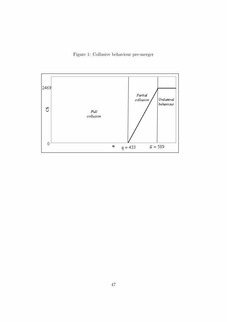
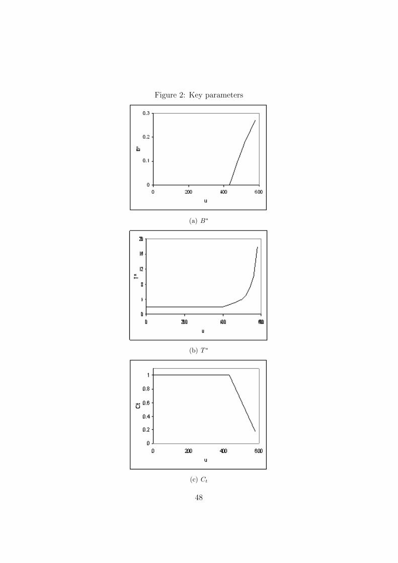
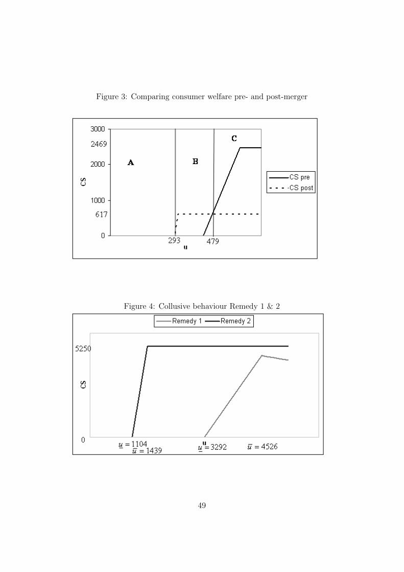

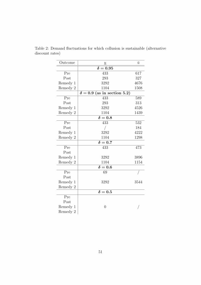
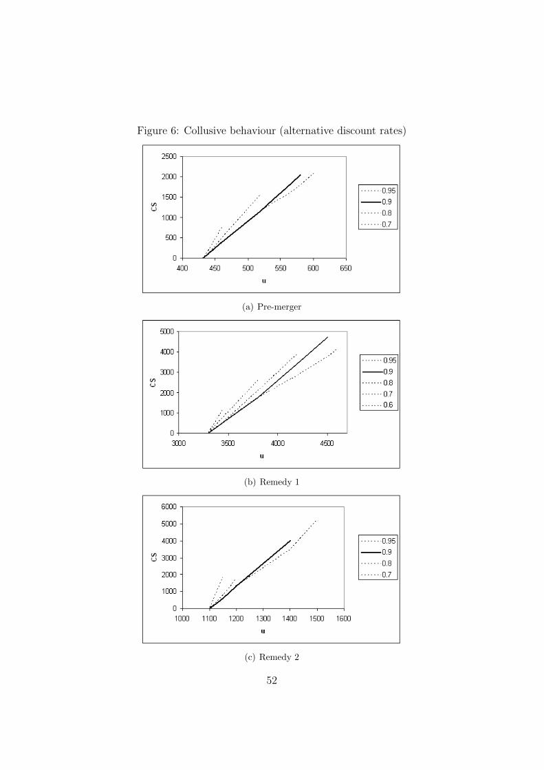


![Unilateral acts of states: Ninth report on unilateral acts ... · 147 UNILATERAL ACTS OF STATES [Agenda item 6] DOCUMENT A/CN.4/569 and Add.1 Ninth report on unilateral acts of States,](https://static.documents.pub/doc/80x56/5f7232786650045f097b30a8/unilateral-acts-of-states-ninth-report-on-unilateral-acts-147-unilateral-acts.jpg)
