UNIT‐1 IntroductionLecture‐1       Motivation: Why data mining?

Lecture‐2       What is data mining?

Lecture‐3       Data Mining: On what kind ofg

data?

Lecture‐4       Data mining functionality

Lecture‐5       Classification of data mining     

systems

L 6 M j i i d i iLecture‐6       Major issues in data mining

1

Unit‐1 Data warehouse and OLAPUnit 1 Data warehouse and OLAP

L t 7 Wh t i d t h ?Lecture‐7 What is a data warehouse? 

Lecture‐8 A multi‐dimensional data model

Lecture‐9  Data warehouse architecture

Lecture‐10&11  Data warehouse implementation

Lecture‐12 From data warehousing to data miningg g

2

Lecture 1Lecture‐1

Motivation: Why data mining?Motivation: Why data mining?

3

Evolution of Database Technology

1960 d li• 1960s and earlier: • Data Collection and Database Creation

– Primitive file processing

4

Evolution of Database Technology

• 1970s ‐ early 1980s: D B M S• Data Base Management Systems– Hieratical and network database systems– Relational database Systems – Query languages: SQL– Transactions, concurrency control and recovery.– On‐line transaction processing (OLTP)On line transaction processing (OLTP)

5

Evolution of Database Technology

• Mid ‐1980s ‐ present:Mid  1980s  present: – Advanced data models 

• Extended relational object relational• Extended relational, object‐relational

– Advanced application‐oriented DBMS ti l i tifi i i t l lti di• spatial, scientific, engineering, temporal, multimedia, 

active, stream and sensor, knowledge‐based

6

Evolution of Database Technology

• Late 1980s‐presentp– Advanced Data Analysis

• Data warehouse and OLAPi i d k l d di• Data mining and knowledge discovery

• Advanced data mining appliations• Data mining and socity

• 1990s‐present: – XML‐based database systems– Integration with information retrieval– Data and information integreation

7

Evolution of Database Technology

• Present – future:Present  future: – New generation of integrated data and information systeminformation system.

8

Lecture‐2What Is Data Mining?What Is Data Mining?

9

What Is Data Mining?

• Data mining refers to extracting or miningData mining refers to extracting or mining knowledge from large amounts of data.

• Mining of gold from rocks or sand• Mining of gold from rocks or sand• Knowledge mining from data, knowledge 

i d / l i dextraction, data/pattern analysis, data archeology, and data dreding.

• Knowledge Discovery from data, or KDD

10

Data Mining: A KDD Process

Pattern Evaluation– Data mining: the core of knowledge discovery process Data Mining

Pattern Evaluation

process.

Task-relevant Data

Data Warehouse Selection

Data Cleaning

Data Integration

Databases

11

Steps of a KDD ProcessSteps of a KDD Process

1 Data cleaning1. Data cleaning2. Data integration3 l i3. Data selection4. Data transformation5. Data mining6 Pattern evaluation6. Pattern evaluation7. Knowledge presentaion

12

Steps of a KDD Processp

• Learning the application domain:l i k l d d l f– relevant prior knowledge and goals of 

application• Creating a target data set: data selection• Creating a target data set: data selection• Data cleaning and preprocessing• Data reduction and transformation:Data reduction and transformation:

– Find useful features, dimensionality/variable reduction, invariant representation.

13

Steps of a KDD ProcessSteps of a KDD Process

• Choosing functions of data miningChoosing functions of data mining – summarization, classification, regression, association, clustering.

• Choosing the mining algorithms• Data mining: search for patterns of interest• Pattern evaluation and knowledge presentation

– visualization, transformation, removing redundant patterns, etc.

• Use of discovered knowledge

14

Architecture of a Typical Data Mi i S tMining System

G hi l i f

Pattern evaluation

Graphical user interface

Data mining engine

Pattern evaluation

Database or data warehouse server

a a g gKnowledge-base

Data

Data cleaning & data integration Filteringwarehouse server

WarehouseDatabases

15

Data Mining and Business IntelligenceData Mining and Business IntelligenceIncreasing potentialto supportto supportbusiness decisions End UserMaking

Decisions

BusinessAnalyst

D t

Data PresentationVisualization Techniques

D t Mi i DataAnalyst

Data MiningInformation Discovery

Data Exploration

DBAOLAP, MDA

Statistical Analysis, Querying and Reporting

Data Warehouses / Data Marts

DBAData Sources

Paper, Files, Information Providers, Database Systems, OLTP

16

Lecture‐3Data Mining: On What Kind of Data?

17

Data Mining: On What Kind of Data?

• Relational databases• Data warehouses• Transactional databases

18

Data Mining: On What Kind of Data?Data Mining: On What Kind of Data?

• Advanced DB and information repositoriesAdvanced DB and information repositories– Object‐oriented and object‐relational databasesSpatial databases– Spatial databases

– Time‐series data and temporal dataT t d t b d lti di d t b– Text databases and multimedia databases

– Heterogeneous and legacy databasesWWW– WWW

19

Lecture‐4Lecture 4Data Mining Functionalities

20

Data Mining Functionalities g

• Concept description: Characterization and p pdiscrimination– Data can be associated with classes or conceptsp– Ex. AllElectronics store classes of items for sale include computer and printers.

– Description of class or concept called class/concept description.

– Data characterization– Data discrimination

21

Data Mining FunctionalitiesData Mining Functionalities

• Mining Frequent Patterns Associations andMining Frequent Patterns, Associations, and Correlations

• Frequent patters‐ patterns occurs frequentlyFrequent patters patterns occurs frequently• Item sets, subsequences and substructures• Frequent item set• Sequential patterns• Structured patterns

22

Data Mining FunctionalitiesData Mining Functionalities

• Association AnalysisAssociation Analysis– Multi‐dimensional vs. single‐dimensional associationassociation 

– age(X, “20..29”) ^ income(X, “20..29K”) => buys(X, “PC”) [ t 2% fid 60%]“PC”) [support = 2%, confidence = 60%]

– contains(T, “computer”)    =>  contains(x, “ f ”) [ f ]“software”) [support=1%, confidence=75%]

23

Data Mining Functionalities

• Classification and Prediction  Finding models (functions) that describe and– Finding models (functions) that describe and distinguish data classes or concepts for predict the class whose label is unknownclass whose label is unknown

– E.g., classify countries based on climate, or classify cars based on gas mileagecars based on gas mileage

– Models: decision‐tree, classification rules (if‐then), l t kneural network

– Prediction: Predict some unknown or missing numerical values 

24

Data Mining FunctionalitiesData Mining Functionalities

• Cluster analysisCluster analysis– Analyze class‐labeled data objects, clustering analyze data objects without consulting a knownanalyze data objects without consulting a known class label.Cl t i b d th i i l i i i th– Clustering based on the principle: maximizing the intra‐class similarity and minimizing the interclass similaritysimilarity

25

Data Mining Functionalities g• Outlier analysis

– Outlier: a data object that does not comply with the general behavior– Outlier: a data object that does not comply with the general behavior of the model of the data

– It can be considered as noise or exception but is quite useful in fraud detection, rare events analysis

• Trend and evolution analysisy

– Trend and deviation:  regression analysis

Sequential pattern mining periodicity analysis– Sequential pattern mining, periodicity analysis

– Similarity‐based analysis

26

Lecture‐5Lecture 5Data Mining: Classification Schemes

27

Data Mining: Confluence of Multiple Disciplines

Database Technology Statistics

Data MiningInformationMachineLearningData MiningScience MachineLearning

OtherDisciplines

VisualizationDisciplines

28

Data Mining: Classification SchemesData Mining: Classification Schemes

• General functionalityy

– Descriptive data mining 

– Predictive data mining– Predictive data mining

• Data mining various criteria's:

– Kinds of databases to be mined

– Kinds of knowledge to be discovered

– Kinds of techniques utilized

– Kinds of applications adaptedpp p

29

Data Mining: Classification Schemes

• Databases to be mined– Relational, transactional, object‐oriented, object‐, , j , jrelational, active, spatial, time‐series, text, multi‐media, heterogeneous, legacy, WWW, etc.

• Knowledge to be minedKnowledge to be mined– Characterization, discrimination, association, classification, clustering, trend, deviation and outlier analysis etcanalysis, etc.

– Multiple/integrated functions and mining at multiple levels

• analysis, Web mining, Weblog analysis, etc.

30

Data Mining: Classification SchemesData Mining: Classification Schemes

• Techniques utilizedTechniques utilized–Database‐oriented, data warehouse (OLAP), machine learning statistics visualizationmachine learning, statistics, visualization, neural network, etc.

A li i d d• Applications adapted–Retail, telecommunication, banking, fraud analysis, DNA mining, stock market

31

Lecture‐6Lecture 6Major Issues in Data Mining

32

Major Issues in Data Mining

• Mining methodology and user interaction issues– Mining different kinds of knowledge in databases– Interactive mining of knowledge at multiple levels of abstraction

– Incorporation of background knowledge– Data mining query languages and ad‐hoc data mining– Expression and visualization of data mining results– Handling noise and incomplete data– Pattern evaluation: the interestingness problem

33

Major Issues in Data MiningMajor Issues in Data Mining

• Performance issuesPerformance issues

Effi i d l bilit f d t i i l ith– Efficiency and scalability of data mining algorithms– Parallel, distributed and incremental mining 

h dmethods

34

Major Issues in Data Mining

• Issues relating to the diversity of data typesg y yp

Handling relational and complex types of data– Handling relational and complex types of data

Minin information from hetero eneo s databases– Mining information from heterogeneous databases and global information systems (WWW)

35

Lecture‐7

Wh t i D t W h ?What is Data Warehouse?

36

What is Data Warehouse?• Defined in many different ways

– A decision support database that is maintained separatelyfrom the organization’s operational databasefrom the organization’s operational database

– Support information processing by providing a solid platform of consolidated, historical data for analysis.

• “A data warehouse is a subject‐oriented, integrated, time‐variant and nonvolatile collection of data in support ofvariant, and nonvolatile collection of data in support of management’s decision‐making process.”—W. H. Inmon

h i• Data warehousing:– The process of constructing and using data warehouses

37

D t W h S bj t O i t dData Warehouse—Subject‐Oriented• Organized around major subjects such as customer productOrganized around major subjects, such as customer, product, 

sales.

• Focusing on the modeling and analysis of data for decision• Focusing on the modeling and analysis of data for decision makers, not on daily operations or transaction processing.

• Provide a simple and concise view around particular subject• Provide a simple and concise view around particular subject issues by excluding data that are not useful in the decision support processsupport process.

38

Data Warehouse—Integrated• Constructed by integrating multiple, heterogeneous data sources– relational databases, flat files, on‐line transaction records

• Data cleaning and data integration techniques are g g qapplied.– Ensure consistency in naming conventions, encoding structures, attribute measures, etc. among different data sources

• E.g., Hotel price: currency, tax, breakfast covered, etc.g , p y, , ,

– When data is moved to the warehouse, it is converted.  

39

Data Warehouse Time VariantData Warehouse—Time Variant• The time horizon for the data warehouse is significantly longer than that of operational systems.– Operational database: current value data.– Data warehouse data: provide information from a historical perspective (e.g., past 5‐10 years)

k i h d h• Every key structure in the data warehouse– Contains an element of time, explicitly or implicitly– But the key of operational data may or may not contain “time element”.

40

Data Warehouse Non VolatileData Warehouse—Non‐Volatile

• A physically separate store of data transformed from the operational environment.

• Operational update of data does not occur in the data warehouse environment.– Does not require transaction processing, recovery, and concurrency control mechanismsy

– Requires only two operations in data accessing: 

• initial loading of data and access of data.t a oad g of data a d access of data

41

Data Warehouse vs Operational DBMSData Warehouse vs. Operational  DBMS• Distinct features (OLTP vs. OLAP):

U d t i t ti t k t– User and system orientation: customer vs. market– Data contents: current, detailed vs. historical, consolidatedDatabase design: ER + application vs star + subject– Database design: ER + application vs. star + subject

– View: current, local vs. evolutionary, integratedAccess patterns: update vs read only but complex queries– Access patterns: update vs. read‐only but complex queries

42

Data Warehouse vs. Operational DBMSData Warehouse vs. Operational DBMS

• OLTP (on‐line transaction processing)– Major task of traditional relational DBMS– Day‐to‐day operations: purchasing, inventory, banking, manufacturing, payroll, registration, accounting, etc.

• OLAP (on‐line analytical processing)– Major task of data warehouse system– Data analysis and decision making

43

OLTP vs OLAPOLTP vs. OLAP OLTP OLAP users clerk, IT professional knowledge worker function day to day operations decision support DB design application-oriented subject-orientedg pp jdata current, up-to-date

detailed, flat relational isolated

historical, summarized, multidimensional integrated, consolidated

usage repetitive ad hocusage repetitive ad-hocaccess read/write

index/hash on prim. key lots of scans

unit of work short, simple transaction complex queryy# records accessed tens millions #users thousands hundreds DB size 100MB-GB 100GB-TBmetric transaction throughput query throughput, response

44

Why Separate Data Warehouse?Why Separate Data Warehouse?• High performance for both systems

– DBMS— tuned for OLTP: access methods, indexing, concurrency control, recovery

W h t d f OLAP l OLAP– Warehouse—tuned for OLAP: complex OLAP queries, multidimensional view, consolidation.

45

Why Separate Data Warehouse?Why Separate Data Warehouse?

• Different functions and different data:Different functions and different data:– missing data: Decision support requires historical data which operational DBs do not typically maintain

– data consolidation:  DS requires consolidation (aggregation summari ation) of data from(aggregation, summarization) of data from heterogeneous sources

– data quality: different sources typically usedata quality: different sources typically use inconsistent data representations, codes and formats which have to be reconciled

46

L 8Lecture‐8

A multi‐dimensional data model

47

Cube: A Lattice of Cuboids

all

time item location supplier

0-D(apex) cuboid

time item location supplier

time item time location item location location supplier

1-D cuboids

time,item time,location

time,supplier

item,location

item,supplier

location,supplier

2-D cuboids

time,item,location

time,item,supplier

time,location,supplier

item,location,supplier

3-D cuboids

time, item, location, supplier

4-D(base) cuboid

48

Conceptual Modeling of Data WarehousesConceptual Modeling of Data Warehouses

• Modeling data warehouses: dimensions & measures– Star schema: A fact table in the middle connected to a set of di i bldimension tables 

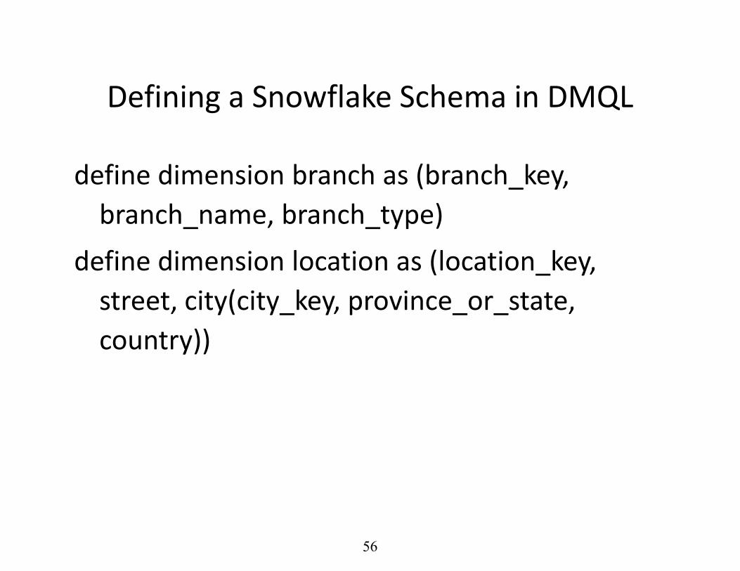
– Snowflake schema:  A refinement of star schema where some dimensional hierarchy is normalized into a set ofsome dimensional hierarchy is normalized into a set of smaller dimension tables, forming a shape similar to snowflakesnowflake

– Fact constellations:  Multiple fact tables share dimension tables, viewed as a collection of stars, therefore called galaxy schema or fact constellation 

49

Example of Star SchemaExample of Star Schema

time key

timeitemtime_key

dayday_of_the_weekmonth

Sales Fact Table

time key

item_keyitem_namebrand

quarteryear

time_key

item_key

branch key

typesupplier_type

location_keystreet

locationbranch_key

location_key

units soldbranch_keybranch name

branch

cityprovince_or_streetcountry

units_sold

dollars_sold

avg_sales

b a c _ a ebranch_type

Measures

50

Example of Snowflake SchemaExample of Snowflake Schema

time key

timeitemtime_key

dayday_of_the_weekmonth

Sales Fact Table

time key

item_keyitem_namebrandt

supplier_keysupplier_type

supplier

quarteryear

time_key

item_key

branch key

typesupplier_key

location_keystreetit k

location_ y

location_key

units_soldbranch_keybranch name

branch

city_keydollars_sold

avg_sales

b a c _ a ebranch_type

city_keycity

city

Measuresy

province_or_streetcountry

51

Example of Fact Constellationp

time_key

timeitem Shipping Fact Table

dayday_of_the_weekmonthquarter

Sales Fact Table

time key

item_keyitem_namebrandtype

time_key

item_keyyear

_ y

item_key

branch_key

ypsupplier_type shipper_key

from_location

location_keystreet

locationlocation_key

units_soldbranch_keybranch_name

branch to_location

dollars_coststreetcityprovince_or_streetcountry

dollars_sold

avg_salesM

branch_type units_shipped

shipperMeasures shipper_key

shipper_namelocation_keyshipper_type

52

A Data Mining Query Language, DMQL: Language PrimitivesPrimitives

• Cube Definition (Fact Table)Cube Definition (Fact Table)define cube <cube_name> [<dimension_list>]:         <measure_list>

• Dimension Definition ( Dimension Table )define dimension <dimension_name> as ( ib bdi i li )(<attribute_or_subdimension_list>)

• Special Case (Shared Dimension Tables)Fi t ti “ b d fi iti ”– First time as “cube definition”

– define dimension <dimension_name> as <dimension name first time> in cube _ _ _<cube_name_first_time>

53

Defining a Star Schema in DMQL

define cube sales star [time, item, branch, location]:_ [ , , , ]dollars_sold = sum(sales_in_dollars), avg_sales = avg(sales_in_dollars), units_sold = count(*)

define dimension time as (time_key, day, day_of_week, month, quarter, year)

define dimension item as (item key item name brand typedefine dimension item as (item_key, item_name, brand, type, supplier_type)

define dimension branch as (branch_key, branch_name, branch_type)

define dimension location as (location_key, street, city, province or state country)province_or_state, country)

54

Defining a Snowflake Schema in DMQL

define cube sales_snowflake [time, item, branch, location]:d ll ld ( l i d ll ) ldollars_sold = sum(sales_in_dollars), avg_sales = avg(sales_in_dollars), units_sold = count(*)

define dimension time as (time key day day of weekdefine dimension time as (time_key, day, day_of_week, month, quarter, year)

define dimension item as (item key item name branddefine dimension item as (item_key, item_name, brand, type, supplier(supplier_key, supplier_type))

55

Defining a Snowflake Schema in DMQLDefining a Snowflake Schema in DMQL

define dimension branch as (branch keydefine dimension branch as (branch_key, branch_name, branch_type)

(define dimension location as (location_key, street, city(city_key, province_or_state, country))

56

Defining a Fact Constellation in DMQLdefine cube sales [time, item, branch, location]:

dollars_sold = sum(sales_in_dollars), avg_sales = ( ) (*)avg(sales_in_dollars), units_sold = count(*)

define dimension time as (time_key, day, day_of_week, month, quarter, year)q , y )

define dimension item as (item_key, item_name, brand, type, supplier_type)

define dimension branch as (branch key branch name branch type)define dimension branch as (branch_key, branch_name, branch_type)define dimension location as (location_key, street, city, 

province_or_state, country)

57

Defining a Fact Constellation in DMQLDefining a Fact Constellation in DMQL

define cube shipping [time, item, shipper, from_location, to_location]:

dollar_cost = sum(cost_in_dollars), unit_shipped = count(*)count( )

define dimension time as time in cube salesdefine dimension item as item in cube salesdefine dimension shipper as (shipper_key, shipper_name, 

location as location in cube sales, shipper_type)define dimension from location as location in cube salesde e d e s o o _ ocat o as ocat o cube sa esdefine dimension to_location as location in cube sales

58

Measures: Three Categories

• distributive: if the result derived by applying the function to n aggregate values is the same as thatfunction to n aggregate values is the same as that derived by applying the function on all the data without partitioningwithout partitioning.

• E.g., count(), sum(), min(), max().

• algebraic: if it can be computed by an algebraic• algebraic: if it can be computed by an algebraic function with M arguments (whereM is a bounded integer) each of which is obtained by applying ainteger), each of which is obtained by applying a distributive aggregate function.

• E g avg() min N() standard deviation()• E.g.,  avg(), min_N(), standard_deviation().

59

Measures: Three CategoriesMeasures: Three Categories

• holistic: if there is no constant bound on theholistic: if there is no constant bound on the storage size needed to describe a sub aggregateaggregate.  

• E.g., median(), mode(), rank().

60

A Concept Hierarchy: Dimension (location)

allall

Europe North_America...region

MexicoCanadaSpainGermany ......country

Vancouver ...

country

TorontoFrankfurtcity Vancouver

M. WindL. Chan

... ...

...office

TorontoFrankfurtcity

M. WindL. Chan ...office

61

M ltidi i l D tMultidimensional Data• Sales volume as a function of product,Sales volume as a function of product, month, and region

Dimensions: Product, Location, TimeHierarchical summarization pathsHierarchical summarization paths

Industry Region Year

oduc

t Category Country Quarter

Product City Month Week

Pro

Office Day

Month

62

A Sample Data CubeA Sample Data CubeTotal annual salesof TV in U S A

Datesum1Qtr 2Qtr 3Qtr 4Qt of TV in U.S.A.

y

sumTV

VCRPC

1Qtr 2Qtr 3Qtr 4QtrU.S.A

Cou

ntrysum

Canada

Mexico CMexico

sum

63

Cuboids Corresponding to the CubeCuboids Corresponding to the Cube

all

d date country0-D(apex) cuboid

product date country

product,date product,country date, country

1-D cuboids

p , p , y , y2-D cuboids

3 D(b ) b idproduct, date, country

3-D(base) cuboid

64

OLAP Operationsp

• Roll up (drill‐up): summarize dataRoll up (drill up): summarize data– by climbing up hierarchy or by

dimension reductiondimension reduction• Drill down (roll down): reverse of roll‐up

f hi h l l t l – from higher level summary to lower level summary or detailed data, or introducing new dimensionsintroducing new dimensions

• Slice and dice: – project and select

65

OLAP OperationsOLAP Operations

• Pivot (rotate):Pivot (rotate): – reorient the cube, visualization, 3D to

series of 2D planes.se es o p a es• Other operations

– drill across: involving (across) more drill across: involving (across) more than one fact table

– drill through: through the bottom level drill through: through the bottom level of the cube to its back-end relational tables (using SQL)

66

Lecture‐9

Data warehouse architecture

67

Steps for the Design and Construction of hData Warehouse

• The design of a data warehouse: a business analysis frameworkanalysis framework

• The process of data warehouse design• A three‐tier data ware house architecture

68

Design of a Data Warehouse: A Business Analysis FrameworkFramework

F i di th d i f d t h• Four views regarding the design of a data warehouse – Top‐down view

• allows selection of the relevant information necessary for the data warehouse

69

Design of a Data Warehouse: A Business Analysis F kFramework

– Data warehouse viewData warehouse view• consists of fact tables and dimension tables

– Data source view• exposes the information being captured stored and• exposes the information being captured, stored, and managed by operational systems

– Business query view • sees the perspectivessees the perspectives

70

Data Warehouse Design ProcessData Warehouse Design Process

• Top‐down, bottom‐up approaches or a combinationTop down, bottom up approaches or a combination of both– Top‐down: Starts with overall design and planning (mature)

– Bottom‐up: Starts with experiments and prototypes (rapid)

• From software engineering point of view– Waterfall: structured and systematic analysis at each step before proceeding to the nextbefore proceeding to the next

– Spiral:  rapid generation of increasingly functional systems, short turn around time, quick turn around

71

Data Warehouse Design ProcessData Warehouse Design Process

• Typical data warehouse design processTypical data warehouse design process– Choose a business process to model, e.g., orders, invoices etcinvoices, etc.

– Choose the grain (atomic level of data) of the business processbusiness process

– Choose the dimensions that will apply to each fact table record

– Choose the measure that will populate each fact table record

72

MultiMulti--Tiered ArchitectureTiered Architecture

Monitor

A l i

Monitor&

IntegratorMetadataother

sources

OLAP Server

DataExtractTransformLoad

AnalysisQueryReportsServe

OperationalDBs

WarehouseLoadRefresh Data mining

Data Marts

OLAP EngineData Sources Front-End ToolsData Storage73

Metadata Repositoryp y• Meta data is the data defining warehouse objects.  It has the 

f ll i ki dfollowing kinds – Description of the structure of the warehouse

• schema, view, dimensions, hierarchies, derived data defn, data mart locations and contents

– Operational meta‐data• data lineage (history of migrated data and transformation path), currency of data (active, archived, or purged), monitoring information (warehouse usage statistics, error reports, audit trails)

– The algorithms used for summarization– The mapping from operational environment to the data warehouse– Data related to system performance

• warehouse schema, view and derived data definitions

– Business data• business terms and definitions, ownership of data, charging policies

74

Data Warehouse Back‐End Tools and Utilities

• Data extraction:– get data from multiple, heterogeneous, and external sources

• Data cleaning:– detect errors in the data and rectify them when possible

• Data transformation:– convert data from legacy or host format to warehouse format

• Load:– sort, summarize, consolidate, compute views, check integrity, and build indices and partitionsintegrity, and build indices and partitions

• Refresh– propagate the updates from the data sources to the warehousewarehouse

75

Three Data Warehouse Models• Enterprise warehouse

– collects all of the information about subjects spanning the entire j p gorganization

• Data Martb f id d h i f l ifi– a subset of corporate‐wide data that is of value to a specific groups 

of users.  Its scope is confined to specific, selected groups, such as marketing data mart

• Independent vs. dependent (directly from warehouse) data mart

• Vi t l h• Virtual warehouse– A set of views over operational databases– Only some of the possible summary views may be materializedy p y y

76

Data Warehouse Development: A Recommended ApproachRecommended Approach

Multi-Tier Data

Distributed Data Marts

Multi-Tier Data Warehouse

E t iData Mart

Data Mart

Enterprise Data Warehouse

Model refinementModel refinement

Define a high-level corporate data model

77

Types of OLAP Servers • Relational OLAP (ROLAP) 

– Use relational or extended‐relational DBMS to store and manage warehouse data and OLAP middle ware to support missing piecesInclude optimization of DBMS backend implementation of– Include optimization of DBMS backend, implementation of aggregation navigation logic, and additional tools and services

– greater scalability

• Multidimensional OLAP (MOLAP) – Array‐based multidimensional storage engine (sparse matrix techniques)fast indexing to pre computed summarized data– fast indexing to pre‐computed summarized data

78

Types of OLAP ServersTypes of OLAP Servers

• Hybrid OLAP (HOLAP)Hybrid OLAP (HOLAP)– User flexibility, e.g.,  low level: relational, high‐level: arraylevel: array

• Specialized SQL serversspecialized support for SQL queries over– specialized support for SQL queries over star/snowflake schemas

79

Lecture‐10 & 11Lecture 10 & 11

Data warehouse implementationData warehouse implementation

80

Efficient Data Cube Computation

• Data cube can be viewed as a lattice of cuboids  Th b tt t b id i th b b id– The bottom‐most cuboid is the base cuboid

– The top‐most cuboid (apex) contains only one cellHow many cuboids in an n dimensional cube with L levels?– How many cuboids in an n‐dimensional cube with L levels?

• Materialization of data cube)1( n

LT• Materialization of data cube– Materialize every (cuboid) (full materialization), none (no materialization) or some (partial materialization)

)11

(

i iLT

materialization), or some (partial materialization)– Selection of which cuboids to materialize

• Based on size, sharing, access frequency, etc., g, q y,

81

Cube Operation• Cube definition and computation in DMQL

define cube sales[item, city, year]: sum(sales_in_dollars)

compute cube sales

• Transform it into a SQL‐like language (with a new operator cubeby introduced by Gray et al ’96)by, introduced by Gray et al. 96)

SELECT item, city, year, SUM (amount)

FROM SALES ()

CUBE BY item, city, year• Need compute the following Group‐Bys

(date product customer)

(item)(city) (year)

(date, product, customer),(date,product),(date, customer), (product, customer),(date), (product), (customer)()

(city, item) (city, year) (item, year)

()

(city, item, year)

82

Cube Computation: ROLAP‐Based Method

• Efficient cube computation methodsp– ROLAP‐based cubing algorithms (Agarwal et al’96)– Array‐based cubing algorithm (Zhao et al’97)

Bottom up computation method (Bayer & Ramarkrishnan’99)– Bottom‐up computation method (Bayer & Ramarkrishnan 99)

• ROLAP‐based cubing algorithms S ti h hi d i ti li d t th– Sorting, hashing, and grouping operations are applied to the dimension attributes in order to reorder and cluster related tuples

– Grouping is performed on some sub aggregates as a “partial grouping step”

– Aggregates may be computed from previously computed t th th f th b f t t blaggregates, rather than from the base fact table

83

Multi‐way Array Aggregation for Cube ComputationCube Computation

• Partition arrays into chunks (a small sub cube which fits in memory). 

• Compressed sparse array addressing: (chunk_id, offset)• Compute aggregates in “multi way” by visiting cube cells in the 

order which minimizes the # of times to visit each cell, and reduces memory access and storage costreduces memory access and storage cost.

84

Multi‐way Array Aggregation for C b C t tiCube Computation

6463626148474645

c3c2

1C

B

29 30 31 32

9

13 14 15 16

c1c 0

b3

b244

28 56

60

B

1 2 3 4

5

9b2

b1

b0

5640

24 5236

20

B

Aa1a0 a2 a3

85

Multi‐Way Array Aggregation for Cube ComputationComputation 

• Method: the planes should be sorted and computed according to their size in ascendingcomputed according to their size in ascending order.– Idea: keep the smallest plane in the main– Idea: keep the smallest plane in the main memory, fetch and compute only one chunk at a time for the largest plane

• Limitation of the method: computing well only for a small number of dimensions– If there are a large number of dimensions, “bottom‐up computation” and iceberg cube computation methods can be exploredcomputation methods can be explored

86

Indexing OLAP Data: Bitmap Index• Index on a particular column• Each value in the column has a bit vector: bit‐op is fast• The length of the bit vector: # of records in the base tableThe length of the bit vector: # of records in the base table• The  i‐th bit is set if the  i‐th row of the base table has the 

value for the indexed column• not suitable for high cardinality domains

Cust Region TypeC1 A i R t il

RecID Retail DealerRecIDAsia Europe America

Base table Index on Region Index on Type

C1 Asia RetailC2 Europe DealerC3 Asia DealerC4 A i R t il

1 1 02 0 13 0 1

1 1 0 02 0 1 03 1 0 0

C4 America RetailC5 Europe Dealer

4 1 05 0 1

4 0 0 15 0 1 0

87

Indexing OLAP Data: Join Indices• Join index: JI(R‐id, S‐id) where R (R‐id, …) 

S (S‐id, …)• Traditional indices map the values to a list of p

record ids– It materializes relational join in JI file and speeds 

up relational join — a rather costly operationp j y p• In data warehouses, join index relates the 

values of the dimensions of a start schema to rows in the fact table.to rows in the fact table.– E.g. fact table: Sales and two dimensions city and 

product• A join index on citymaintains for each distinctA join index on citymaintains for each distinct city a list of R‐IDs of the tuples recording the Sales in the city 

– Join indices can span multiple dimensions

88

Efficient Processing OLAP Queries

• Determine which operations should be performed on 

the available cuboids:the available cuboids:

– transform drill, roll, etc. into corresponding SQL and/or OLAP 

i di l i j ioperations, e.g, dice = selection + projection

• Determine to which materialized cuboid(s) the relevant 

operations should be applied.

E l i i d i t t d d• Exploring indexing structures and compressed vs. 

dense array structures in MOLAP

89

Lecture‐12

From data warehousing to dataFrom data warehousing to data 

i imining

90

Data Warehouse Usage

• Three kinds of data warehouse applications– Information processingInformation processing

• supports querying, basic statistical analysis, and reporting using crosstabs, tables, charts and graphsl l– Analytical processing

• multidimensional analysis of data warehouse data• supports basic OLAP operations, slice‐dice, drilling, pivotingpp p , , g, p g

– Data mining• knowledge discovery from hidden patterns • supports associations, constructing analytical models, performing classification and prediction, and presenting the mining results using visualization tools.

• Differences among the three tasks

91

From On‐Line Analytical Processing to On Line Analytical Mining (OLAM)Mining (OLAM)

• Why online analytical mining?Why online analytical mining?– High quality of data in data warehouses

• DW contains integrated, consistent, cleaned datal bl f d d– Available information processing structure surrounding data 

warehouses• ODBC, OLEDB, Web accessing, service facilities, reporting and O lOLAP tools

– OLAP‐based exploratory data analysis• mining with drilling, dicing, pivoting, etc.

– On‐line selection of data mining functions• integration and swapping of multiple mining functions, algorithms, and tasks.g ,

• Architecture of OLAM

92

An OLAM ArchitectureL 4Mi i Mi i l

User GUI API

Layer4

User InterfaceMining query Mining result

OLAMEngine

OLAPEngine

User GUI APILayer3

OLAP/OLAMg g

Data Cube API

Meta Data

MDDBLayer2

MDDBMeta Data

Database APILayer1

Filtering&Integration Filtering

Data Warehouse

Data cleaning

Data integration

y

Data Repository

Databases

93