42
Unit 10 : Advanced Hydrogeology Equations of Mass Transport
| Date post: | 19-Dec-2015 |
| Category: |
Documents |
| View: | 232 times |
| Download: | 6 times |
Unit 10 : Advanced Hydrogeology
Equations of Mass Transport
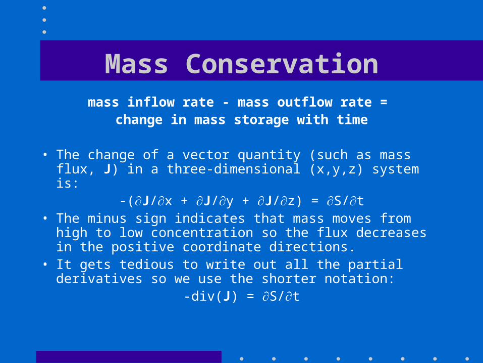
Mass Conservationmass inflow rate - mass outflow rate =
change in mass storage with time
• The change of a vector quantity (such as mass flux, J) in a three-dimensional (x,y,z) system is:
-(J/x + J/y + J/z) = S/t• The minus sign indicates that mass moves from high to
low concentration so the flux decreases in the positive coordinate directions.
• It gets tedious to write out all the partial derivatives so we use the shorter notation:
-div(J) = S/t

Diffusion Equation• The mass in storage in a unit volume of a porous medium is
the concentration (C) times the porosity (n) so we can write:
-div(J) = (Cn)/t
• Suppose our transport process is diffusion, then the mass flux J is given by:
J = -nDd*grad(C)
where grad(C) is short for C/x + C/y + C/z
• The diffusion equation is thus:
div[nDd*grad(C)] = (Cn)/t
or in more concise notation using the operator:
[nDd* (C)] = (Cn)/t
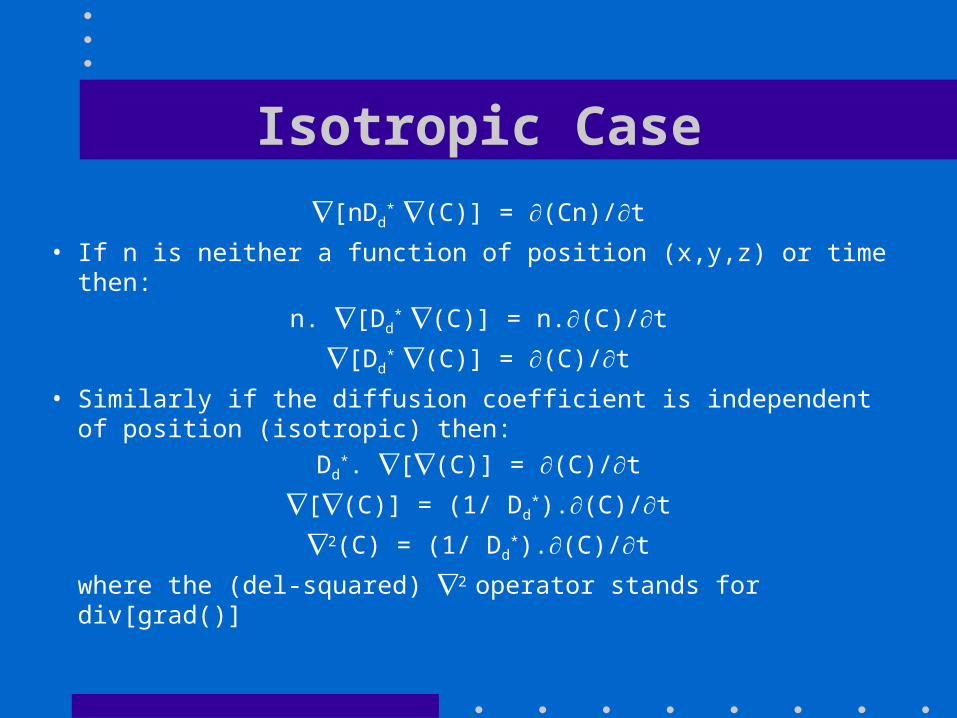
Isotropic Case
[nDd* (C)] = (Cn)/t
• If n is neither a function of position (x,y,z) or time then:
n. [Dd* (C)] = n.(C)/t
[Dd* (C)] = (C)/t
• Similarly if the diffusion coefficient is independent of position (isotropic) then:
Dd*. [(C)] = (C)/t
[(C)] = (1/ Dd*).(C)/t
2(C) = (1/ Dd*).(C)/t
where the (del-squared) 2 operator stands for div[grad()]
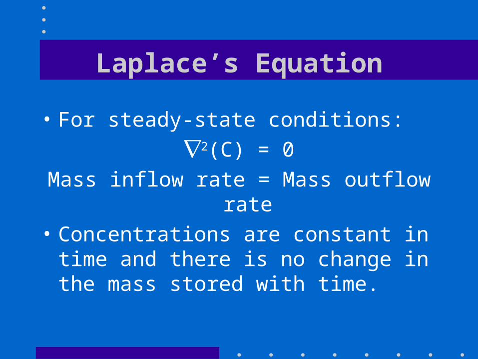
Laplace’s Equation
• For steady-state conditions:
2(C) = 0
Mass inflow rate = Mass outflow rate
• Concentrations are constant in time and there is no change in the mass stored with time.
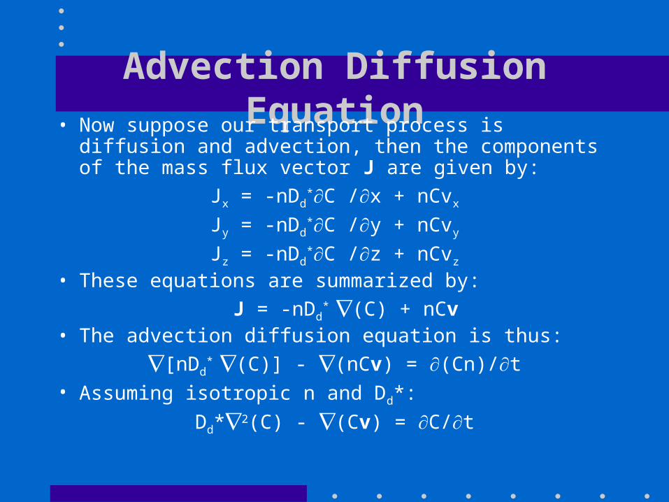
Advection Diffusion Equation• Now suppose our transport process is diffusion and
advection, then the components of the mass flux vector J are given by:
Jx = -nDd*C /x + nCvx
Jy = -nDd*C /y + nCvy
Jz = -nDd*C /z + nCvz
• These equations are summarized by:
J = -nDd* (C) + nCv
• The advection diffusion equation is thus:
[nDd* (C)] - (nCv) = (Cn)/t
• Assuming isotropic n and Dd*:
Dd*2(C) - (Cv) = C/t
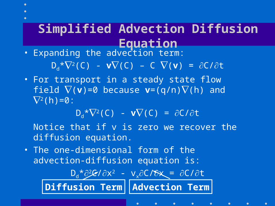
Simplified Advection Diffusion Equation• Expanding the advection term:
Dd*2(C) - v(C) – C (v) = C/t
• For transport in a steady state flow field (v)=0 because v=(q/n)(h) and 2(h)=0:
Dd*2(C) - v(C) = C/t
Notice that if v is zero we recover the diffusion equation.
• The one-dimensional form of the advection-diffusion equation is:
Dd*2C/x2 - vxC/x = C/t
Diffusion Term Advection Term
Dimensionless Form
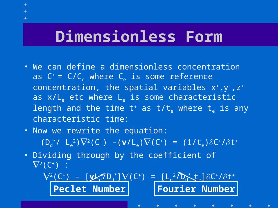
• We can define a dimensionless concentration as C+ = C/Ce where Ce is some reference concentration, the spatial variables x+,y+,z+ as x/Le etc where Le is some characteristic length and the time t+ as t/te where te is any characteristic time:
• Now we rewrite the equation:
(Dd*/ Le
2)2(C+) –(v/Le)(C+) = (1/te)C+/t+
• Dividing through by the coefficient of 2(C+) :
2(C+) – [vLe/Dd*](C+) = [Le
2/Dd* te]C+/t+
Peclet Number Fourier Number
Peclet Number
• The Peclet Number NPE = [vLe/Dd*] is a dimensionless
expression corresponding to the ratio of mass transport by bulk fluid motion (advection) to mass transport by diffusion.
• It is easy to see that a large Peclet Number is characteristic of an advective system and that as the advective velocity (v) approaches zero the system become diffusion dominated.
• The characteristic length Le is arbitrary. Often a characteristic of the porous medium is chosen such as mean pore diameter. Sometimes a numerical grid spacing is selected.
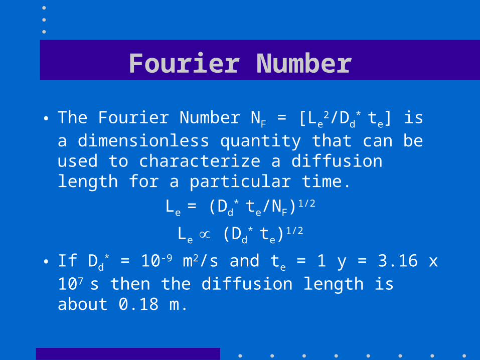
Fourier Number
• The Fourier Number NF = [Le2/Dd
* te] is a dimensionless quantity that can be used to characterize a diffusion length for a particular time.
Le = (Dd* te/NF)1/2
Le (Dd* te)1/2
• If Dd* = 10-9 m2/s and te = 1 y = 3.16 x 10⁷ s
then the diffusion length is about 0.18 m.
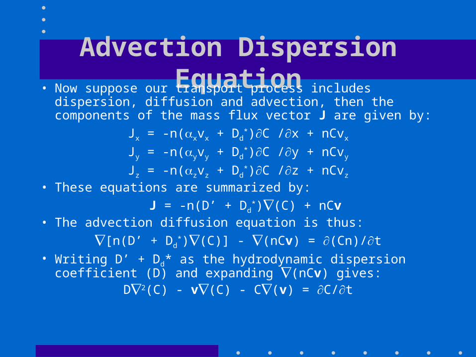
Advection Dispersion Equation• Now suppose our transport process includes dispersion,
diffusion and advection, then the components of the mass flux vector J are given by:
Jx = -n(xvx + Dd*)C /x + nCvx
Jy = -n(yvy + Dd*)C /y + nCvy
Jz = -n(zvz + Dd*)C /z + nCvz
• These equations are summarized by:
J = -n(D’ + Dd*)(C) + nCv
• The advection diffusion equation is thus:
[n(D’ + Dd*)(C)] - (nCv) = (Cn)/t
• Writing D’ + Dd* as the hydrodynamic dispersion coefficient (D) and expanding (nCv) gives:
D2(C) - v(C) - C(v) = C/t

Simplified Advection Dispersion EquationD2(C) - v(C) – C (v) = C/t
• For transport in a steady state flow field (v)=0 because v=(q/n)(h) and 2(h)=0:
D2(C) - v(C) = C/tNotice that if v is zero we recover the diffusion equation because D’ = .v = 0 also.
• The one-dimensional form of the advection-dispersion equation is:
D2C/x2 - vxC/x = C/t
• This equation is the “workhorse” of modelling studies in groundwater contamination.
Dispersion Term Advection Term
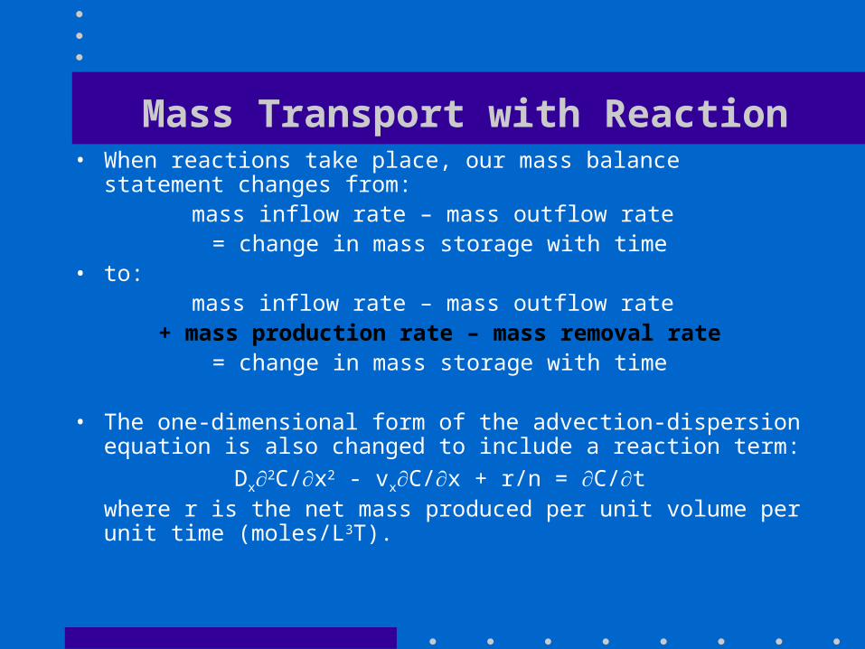
Mass Transport with Reaction• When reactions take place, our mass balance statement changes
from:mass inflow rate – mass outflow rate = change in mass storage with time
• to:mass inflow rate – mass outflow rate
+ mass production rate – mass removal rate= change in mass storage with time
• The one-dimensional form of the advection-dispersion equation is also changed to include a reaction term:
Dx2C/x2 - vxC/x + r/n = C/twhere r is the net mass produced per unit volume per unit time (moles/L3T).
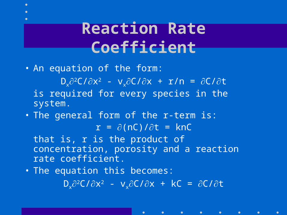
Reaction Rate Coefficient
• An equation of the form:
Dx2C/x2 - vxC/x + r/n = C/tis required for every species in the system.
• The general form of the r-term is:r = (nC)/t = knC
that is, r is the product of concentration, porosity and a reaction rate coefficient.
• The equation this becomes:
Dx2C/x2 - vxC/x + kC = C/t
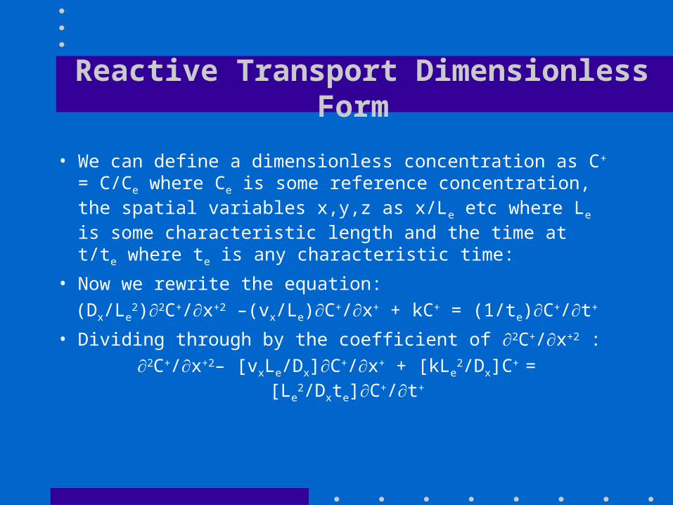
Reactive Transport Dimensionless Form
• We can define a dimensionless concentration as C+ = C/Ce where Ce is some reference concentration, the spatial variables x,y,z as x/Le etc where Le is some characteristic length and the time at t/te where te is any characteristic time:
• Now we rewrite the equation:
(Dx/Le2)2C+/x+2 –(vx/Le)C+/x+ + kC+ = (1/te)C+/t+
• Dividing through by the coefficient of 2C+/x+2 :
2C+/x+2– [vxLe/Dx]C+/x+ + [kLe2/Dx]C+ = [Le
2/Dxte]C+/t+

Dimensionless Numbers• The equation can be written:
2C+/x+2– NPEC+/x+ + DaIIC+ = NFC+/t+
where NPE is the Pelcet number [vxLe/Dx]
NF is the Fourier number [Le2/Dxte]
DaII is the second Damköhler number [kLe2/Dx]
• Another dimensionless Damköhler Number (DaI) can be defined by the equation:
2C+/x+2– NPEC+/x+ + NPEDaIC+ = NFC+/t+
where DaI is the first Damköhler number [kLe/v]
Damköhler Numbers
• The first Damköhler number (DaI) and measures the tendency for reaction relative to the tendency for advective transport.
• The second Damköhler number (DaII) and measures the tendency for reaction relative to the tendency for diffusive transport.
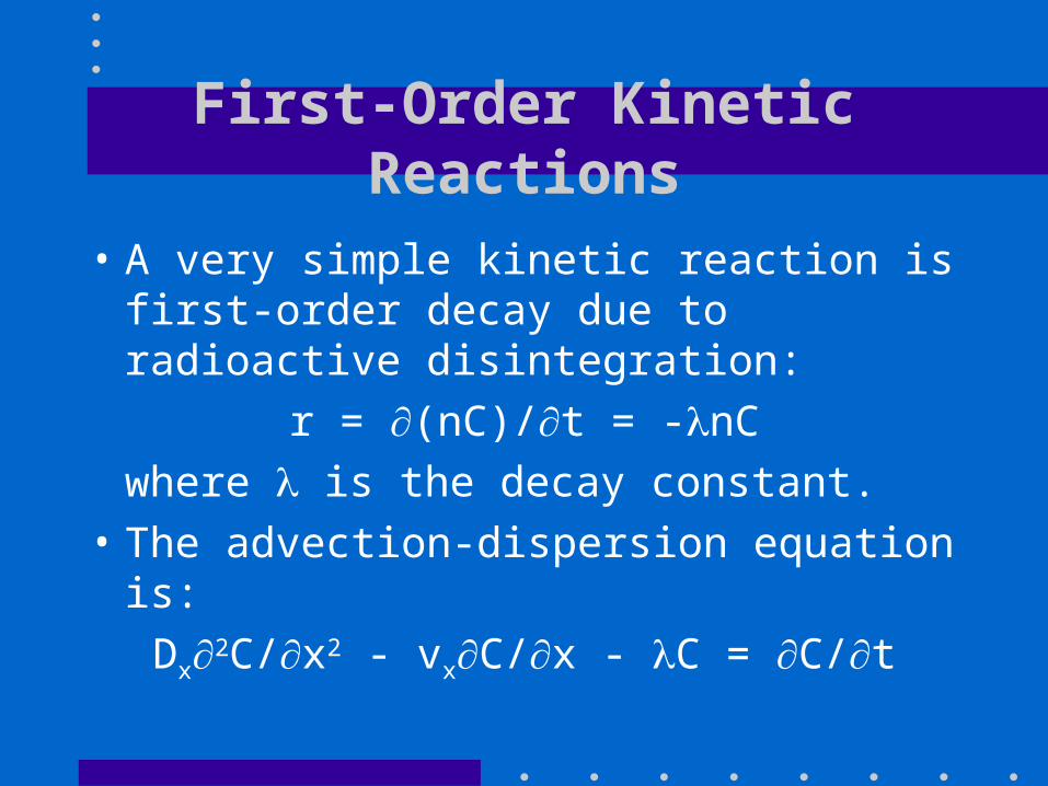
First-Order Kinetic Reactions
• A very simple kinetic reaction is first-order decay due to radioactive disintegration:
r = (nC)/t = -nC
where is the decay constant.
• The advection-dispersion equation is:
Dx2C/x2 - vxC/x - C = C/t
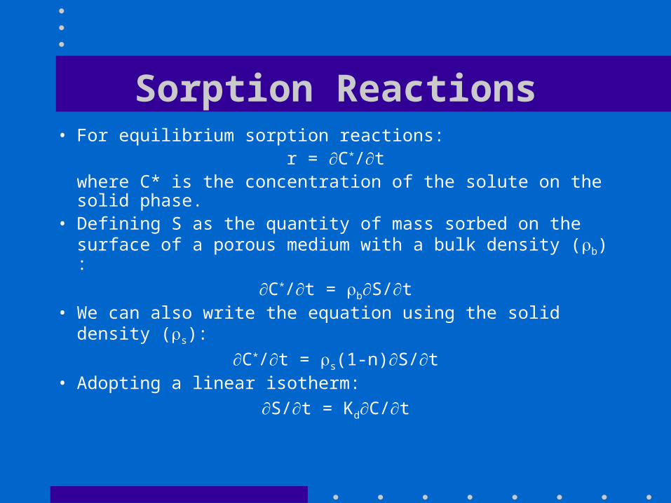
Sorption Reactions• For equilibrium sorption reactions:
r = C*/twhere C* is the concentration of the solute on the solid phase.
• Defining S as the quantity of mass sorbed on the surface of a porous medium with a bulk density (b) :
C*/t = bS/t• We can also write the equation using the solid density (s):
C*/t = s(1-n)S/t• Adopting a linear isotherm:
S/t = KdC/t
Retardation Factor
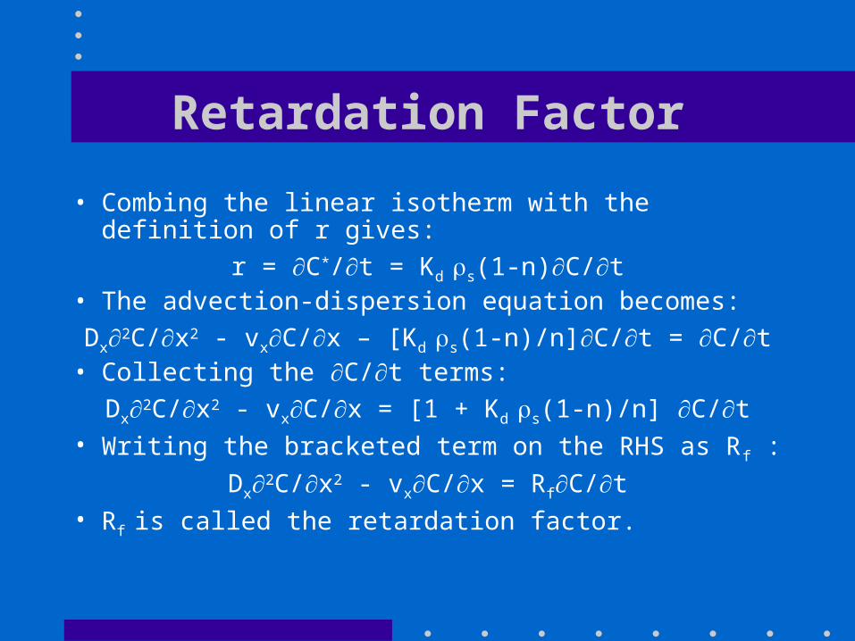
• Combing the linear isotherm with the definition of r gives:
r = C*/t = Kd s(1-n)C/t• The advection-dispersion equation becomes:
Dx2C/x2 - vxC/x – [Kd s(1-n)/n]C/t = C/t• Collecting the C/t terms:
Dx2C/x2 - vxC/x = [1 + Kd s(1-n)/n] C/t• Writing the bracketed term on the RHS as Rf :
Dx2C/x2 - vxC/x = RfC/t• Rf is called the retardation factor.
Retardation Equation
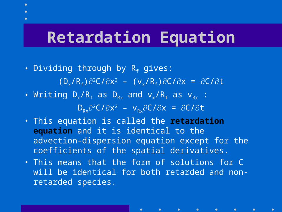
• Dividing through by Rf gives:
(Dx/Rf)2C/x2 – (vx/Rf)C/x = C/t
• Writing Dx/Rf as DRx and vx/Rf as vRx :
DRx2C/x2 – vRxC/x = C/t
• This equation is called the retardation equation and it is identical to the advection-dispersion equation except for the coefficients of the spatial derivatives.
• This means that the form of solutions for C will be identical for both retarded and non-retarded species.
Solid-Solution Reactions
• Reactions between solids and solutions involve many steps.
• In general, the rate of reaction is controlled by the slowest step in the reaction path.
• The reaction may be transport controlled or surface controlled depending on the relative speed of movement of the fluid past the solid surface.
Transport Controlled Reaction Model
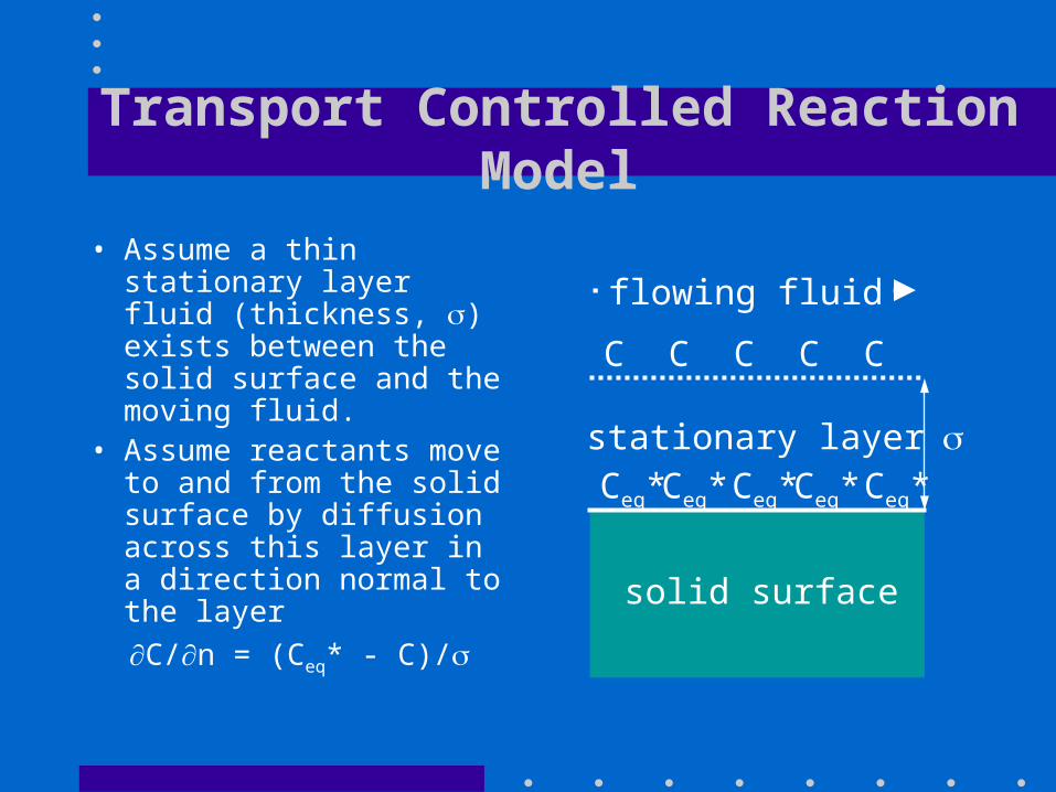
• Assume a thin stationary layer fluid (thickness, ) exists between the solid surface and the moving fluid.
• Assume reactants move to and from the solid surface by diffusion across this layer in a direction normal to the layer
C/n = (Ceq* - C)/
solid surface
Ceq*Ceq* Ceq*Ceq* Ceq*
CC C C C
stationary layer
flowing fluid
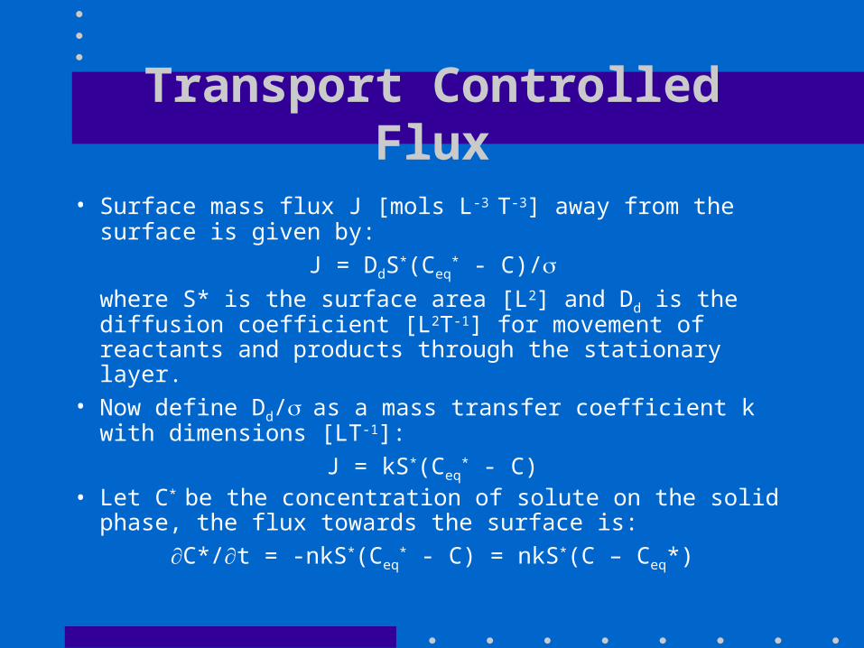
Transport Controlled Flux
• Surface mass flux J [mols L-3 T-3] away from the surface is
given by:
J = DdS*(Ceq* - C)/
where S* is the surface area [L2] and Dd is the diffusion coefficient [L2T-1] for movement of reactants and products through the stationary layer.
• Now define Dd/as a mass transfer coefficient k with dimensions [LT-1]:
J = kS*(Ceq* - C)
• Let C* be the concentration of solute on the solid phase, the flux towards the surface is:
C*/t = -nkS*(Ceq* - C) = nkS*(C – Ceq*)
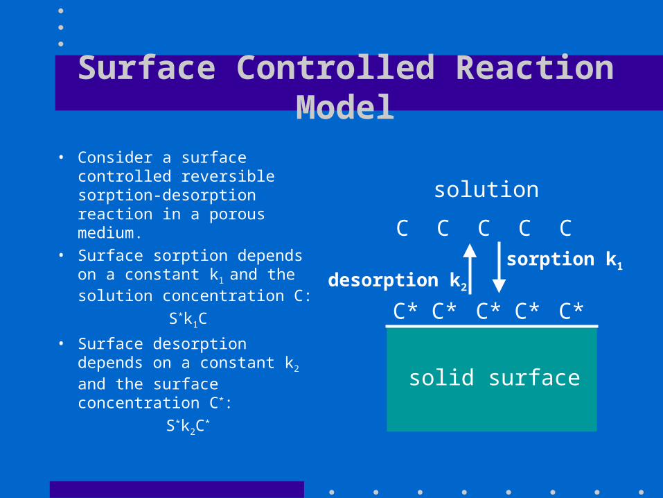
Surface Controlled Reaction Model
• Consider a surface controlled reversible sorption-desorption reaction in a porous medium.
• Surface sorption depends on a constant k1 and the solution concentration C:
S*k1C
• Surface desorption depends on a constant k2 and the surface concentration C*:
S*k2C*
solid surface
C*C* C* C* C*
CC C C C
solution
sorption k1
desorption k2
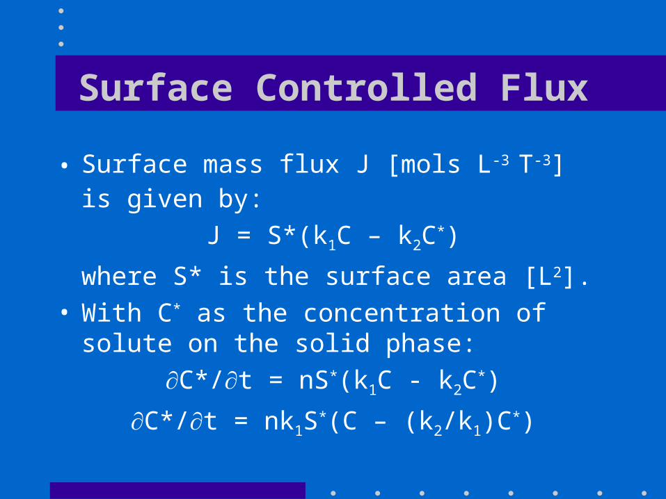
Surface Controlled Flux
• Surface mass flux J [mols L-3 T-3] is given by:
J = S*(k1C – k2C*)
where S* is the surface area [L2].• With C* as the concentration of solute on the
solid phase:
C*/t = nS*(k1C - k2C*)
C*/t = nk1S*(C – (k2/k1)C*)
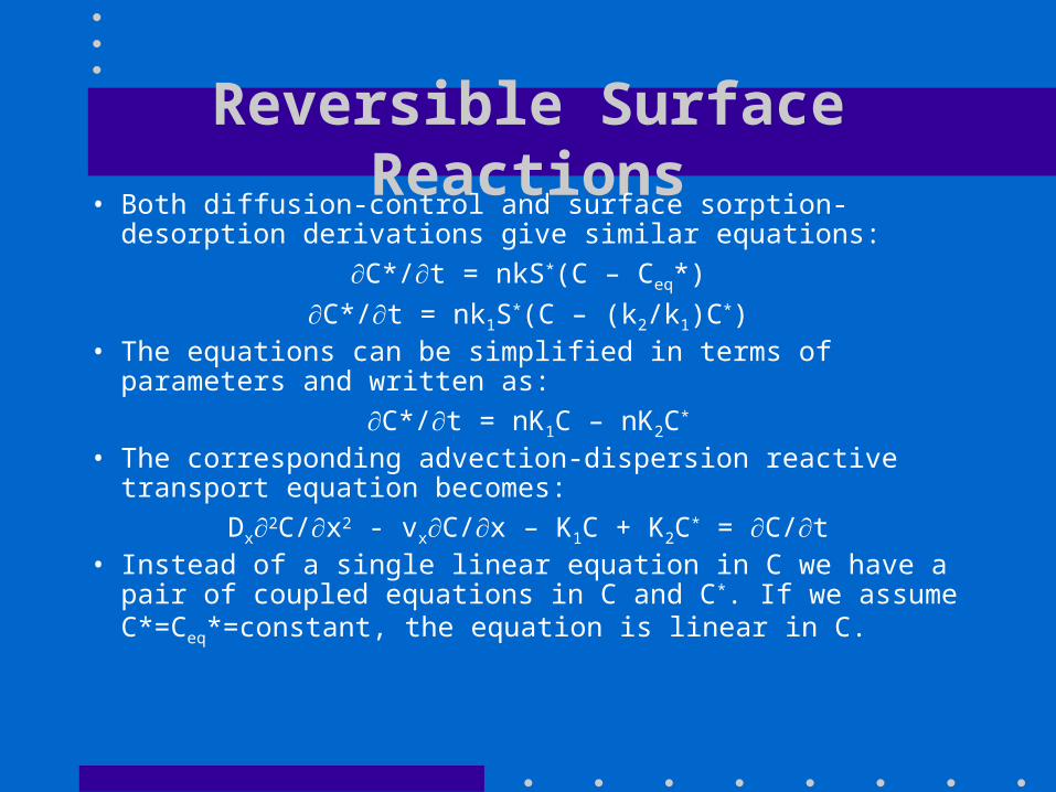
Reversible Surface Reactions• Both diffusion-control and surface sorption-desorption derivations
give similar equations:
C*/t = nkS*(C – Ceq*)
C*/t = nk1S*(C – (k2/k1)C*)• The equations can be simplified in terms of parameters and
written as:
C*/t = nK1C – nK2C*
• The corresponding advection-dispersion reactive transport equation becomes:
Dx2C/x2 - vxC/x – K1C + K2C* = C/t• Instead of a single linear equation in C we have a pair of coupled
equations in C and C*. If we assume C*=Ceq*=constant, the equation is linear in C.
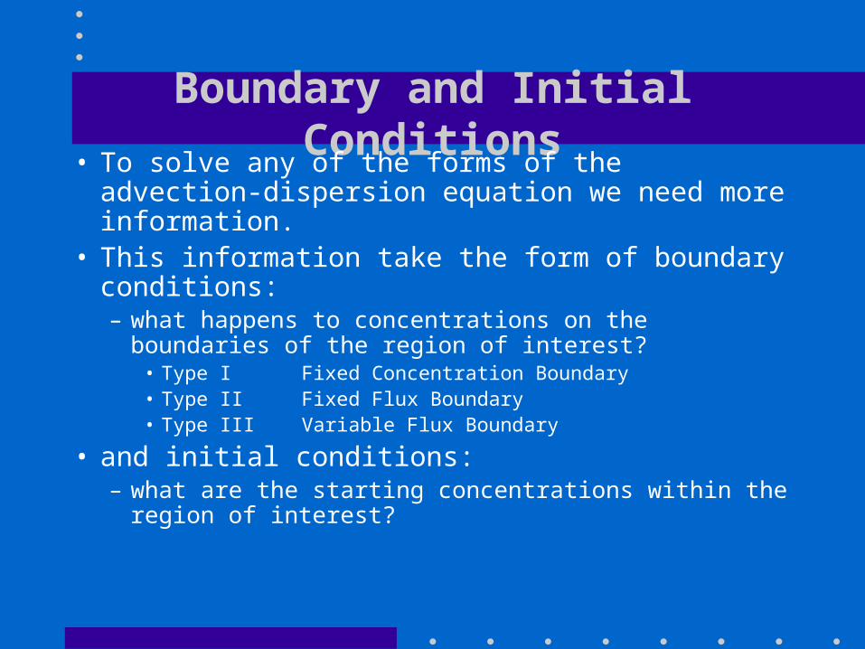
Boundary and Initial Conditions• To solve any of the forms of the advection-
dispersion equation we need more information.• This information take the form of boundary
conditions:– what happens to concentrations on the boundaries of the
region of interest?• Type I Fixed Concentration Boundary• Type II Fixed Flux Boundary• Type III Variable Flux Boundary
• and initial conditions:– what are the starting concentrations within the region of
interest?
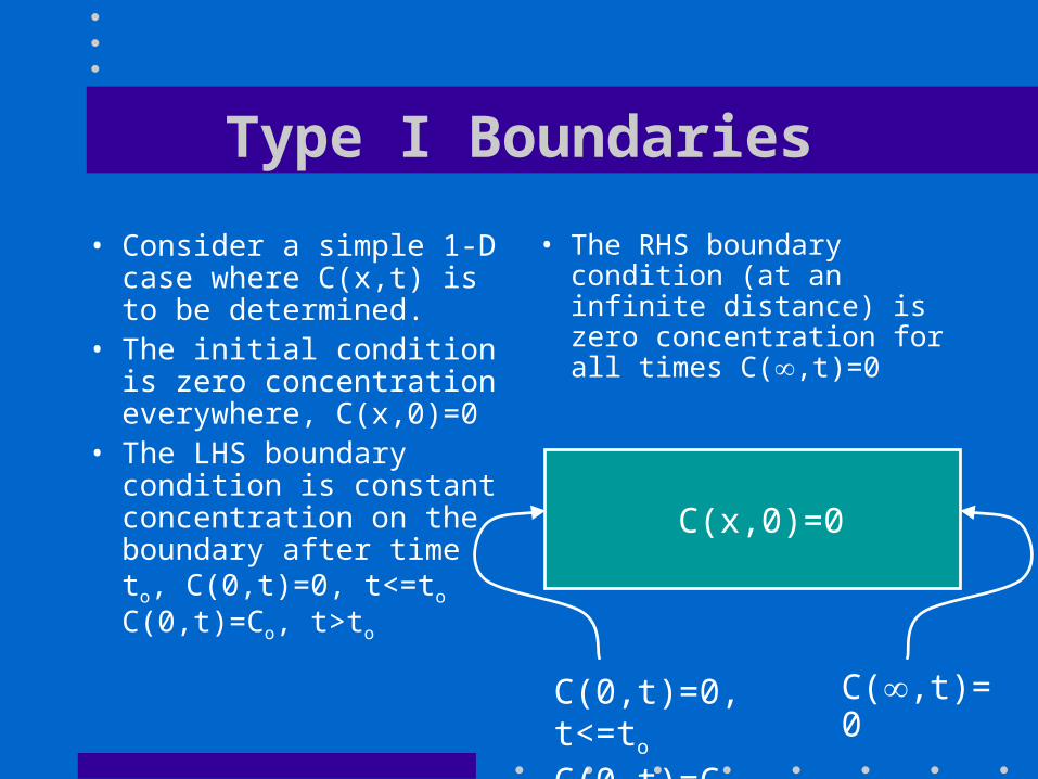
Type I Boundaries
• Consider a simple 1-D case where C(x,t) is to be determined.
• The initial condition is zero concentration everywhere, C(x,0)=0
• The LHS boundary condition is constant concentration on the boundary after time to, C(0,t)=0, t<=to C(0,t)=Co, t>to
• The RHS boundary condition (at an infinite distance) is zero concentration for all times C(,t)=0
C(x,0)=0
C(0,t)=0, t<=to
C(0,t)=Co, t>to
C(,t)=0
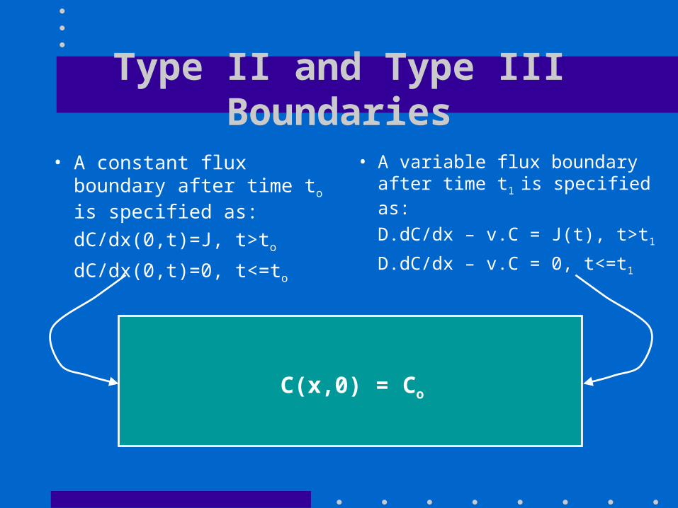
Type II and Type III Boundaries
• A constant flux boundary after time to is specified as:
dC/dx(0,t)=J, t>to
dC/dx(0,t)=0, t<=to
• A variable flux boundary after time t1 is specified as:
D.dC/dx – v.C = J(t), t>t1
D.dC/dx – v.C = 0, t<=t1
C(x,0) = Co
Column with Constant Source
• The concentration distribution in a column is a useful solution of the one-dimensional advection-dispersion equation:
Dx2C/x2 - vxC/x = C/t
• The boundary conditions are C(0,t) = Co
(concentration Co applied at x=0 for all times)
• The initial conditions are C(x,0) = 0 (concentration zero everywhere)
Ogata-Banks Solution
• The solution is provided by Ogata and Banks (1961):
C(x,t) = (Co/2).{ erfc[(x-vxt)/2(Dxt)1/2] + exp(vxx/Dx).erfc[(x+vxt)/2(Dxt)1/2] }
where erfc() is called the complementary error function (1 – erf()).
• The second term in the solution involving the exponential function is almost always small and can be neglected.
• The simplified solution becomes:
C(x,t) = (Co/2).erfc[(x-vxt)/2(Dxt)1/2]
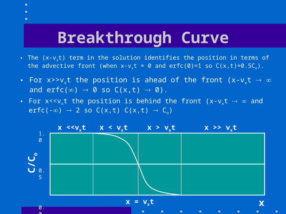
Breakthrough Curve• The (x-vxt) term in the solution identifies the position in terms of the advective
front (when x-vxt = 0 and erfc(0)=1 so C(x,t)=0.5Co).
x
C/C
o
1.0
0.5
0.0
x = vxt
x > vxtx < vxtx <<vxt x >> vxt
• For x>>vxt the position is ahead of the front (x-vxt and erfc() 0 so C(x,t) 0).
• For x<<vxt the position is behind the front (x-vxt and erfc(-) 2 so C(x,t) C(x,t) Co)

Retardation Solution• The simplified Ogata-Banks solution for retarded species
becomes:
C(x,t) = (Co/2).erfc[(x-{vx/Rf}t)/2({Dx/Rf}t)1/2]
which simplifies to:
C(x,t) = (Co/2).erfc[(Rfx-vxt)/2(RfDxt)1/2]
• The effect of retardation for a constant continuous source is to delay breakthrough at position x from time tb to time Rf.tb
C/C
o
1.0
0.5
0.0x = vxtx = vxt/Rf
Retarded species
Unretarded species
Bear Solution• The one-dimensional form of the advection-
dispersion equation for radioactive decay (and biodegradation) is:
Dx2C/x2 - vxC/x - C = C/t• Bear (1979) provides an analytical solution with initial
and boundary conditions C(x,0)=0 and C(0,t)=Co:
C(x,t) = (Co/2).{exp(vxx/Dx)[1 - ]}.erfc[(x-vxt/2(Dxt)1/2]
where (1+4Dx/vx2)1/2
• Note that for =0, =1 and the exponential term disappears and the Bear solution becomes Ogata-Banks solution.
Radioactive Decay Solution• The dimensional group form 4Dx/vx
2 = 4x/vx controls for finite values of . The second form is readily recognized as the first Damköhler number (DaI) withx as the characteristic length.
(1+4Dx/vx2)1/2
• As the half-life of an element gets larger = ln(2)/t1/2 gets smaller as does DaI.
• For long half-lives where is small, is near 1, DaI becomes large and the behaviour is similar to the Ogata-Banks solution.
The solute mass is transported faster than it decays.
• For short half-lives (such as 3H) is relatively large, DaI is small and with >1 the negative exponential term reduces the concentration significantly.
The solute mass decays faster than it is transported.
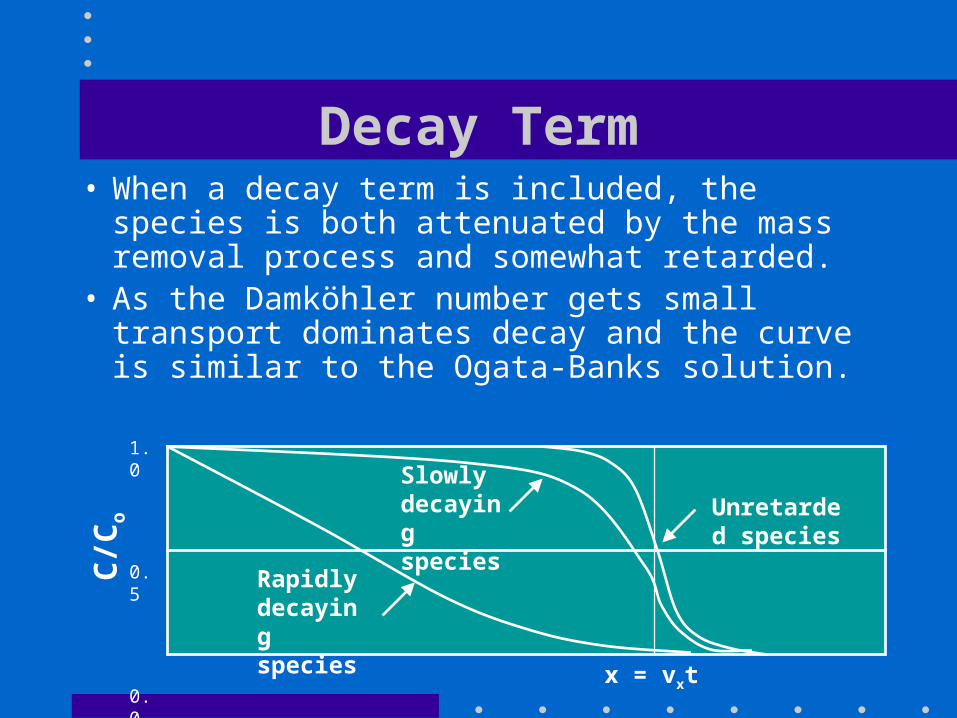
Decay Term• When a decay term is included, the species is
both attenuated by the mass removal process and somewhat retarded.
• As the Damköhler number gets small transport dominates decay and the curve is similar to the Ogata-Banks solution.
C/C
o
1.0
0.5
0.0x = vxt
Unretarded species
Rapidlydecaying species
Slowlydecaying species
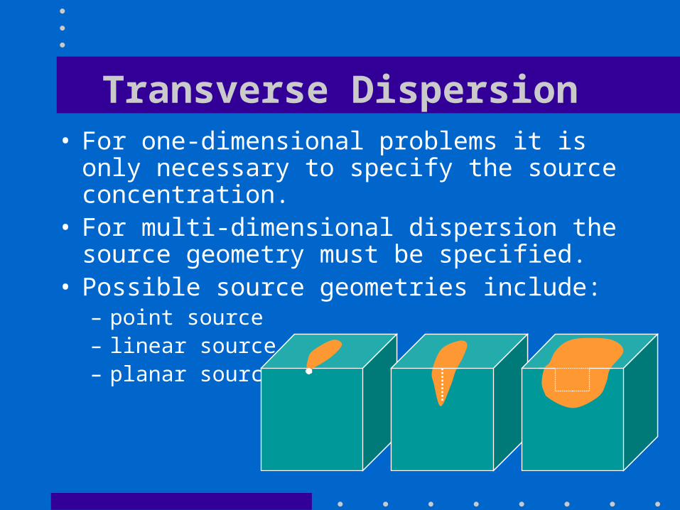
Transverse Dispersion• For one-dimensional problems it is only
necessary to specify the source concentration.
• For multi-dimensional dispersion the source geometry must be specified.
• Possible source geometries include:– point source– linear source– planar source
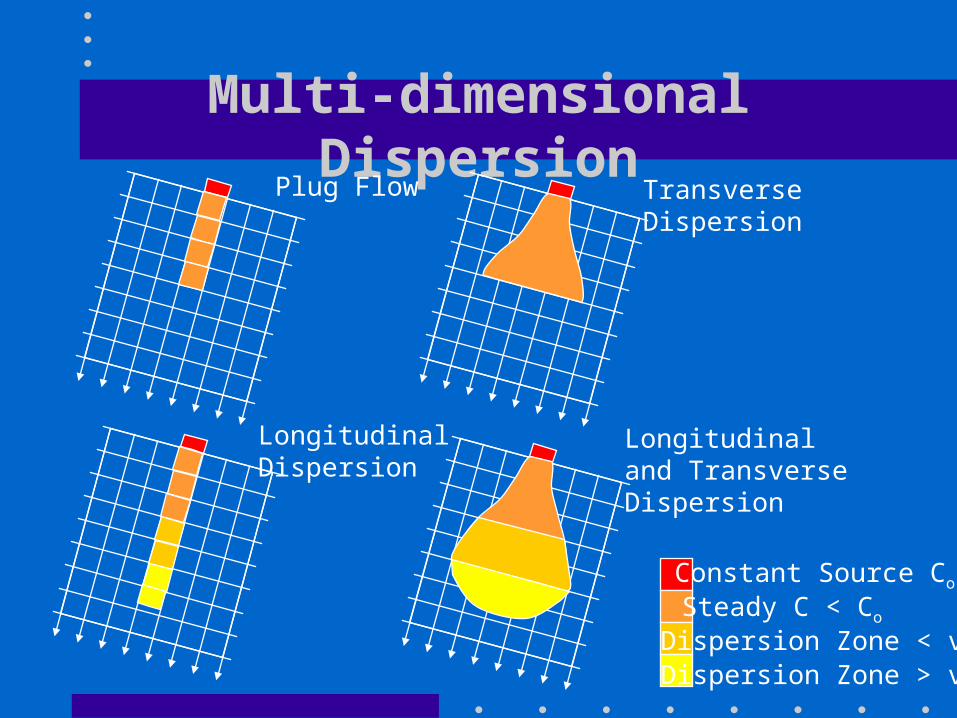
Multi-dimensional Dispersion
Longitudinal Dispersion
TransverseDispersion
Longitudinaland Transverse Dispersion
Plug Flow
Constant Source Co
Steady C < Co
Dispersion Zone < vtDispersion Zone > vt
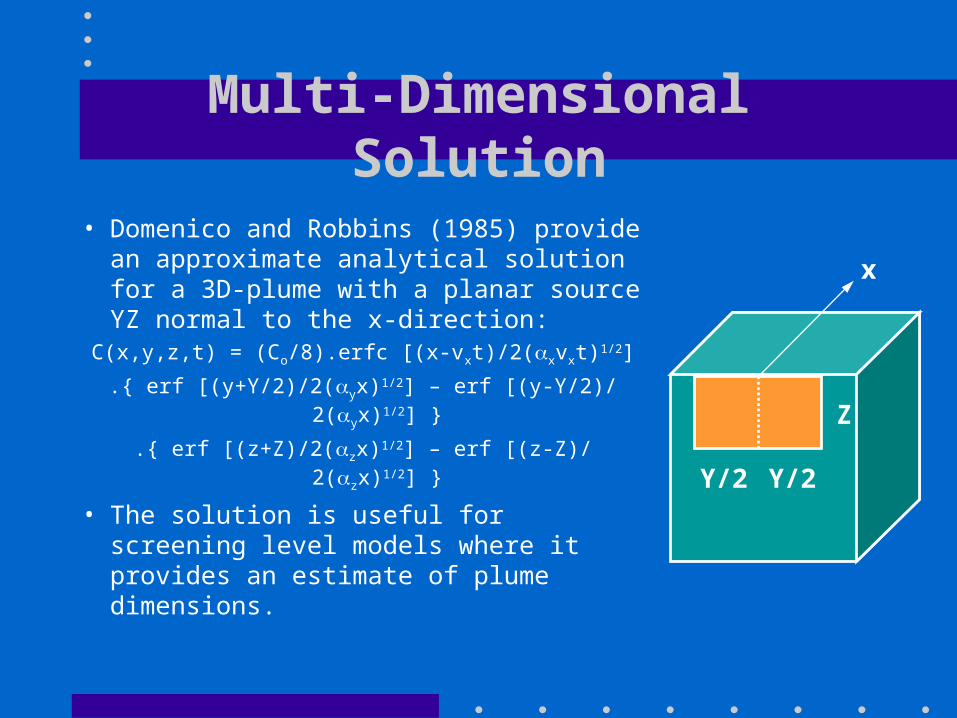
Multi-Dimensional Solution
• Domenico and Robbins (1985) provide an approximate analytical solution for a 3D-plume with a planar source YZ normal to the x-direction:C(x,y,z,t) = (Co/8).erfc [(x-vxt)/2(xvxt)1/2]
.{ erf [(y+Y/2)/2(yx)1/2] – erf [(y-Y/2)/ 2(yx)1/2] }
.{ erf [(z+Z)/2(zx)1/2] – erf [(z-Z)/ 2(zx)1/2] }
• The solution is useful for screening level models where it provides an estimate of plume dimensions.
Y/2 Y/2
Z
x
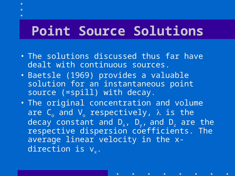
Point Source Solutions
• The solutions discussed thus far have dealt with continuous sources.
• Baetsle (1969) provides a valuable solution for an instantaneous point source (=spill) with decay.
• The original concentration and volume are Co and Vo respectively, is the decay constant and Dx, Dy, and Dz are the respective dispersion coefficients. The average linear velocity in the x-direction is vx.
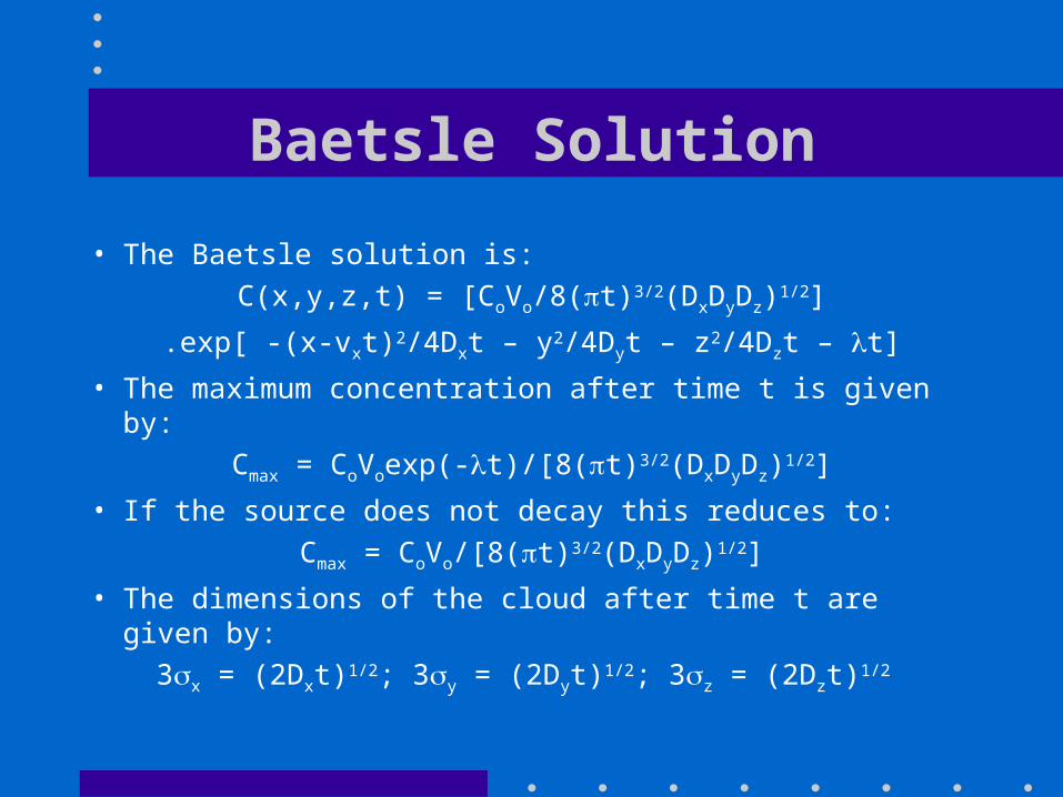
Baetsle Solution
• The Baetsle solution is:
C(x,y,z,t) = [CoVo/8(t)3/2(DxDyDz)1/2]
.exp[ -(x-vxt)2/4Dxt – y2/4Dyt – z2/4Dzt – t]
• The maximum concentration after time t is given by:
Cmax = CoVoexp(-t)/[8(t)3/2(DxDyDz)1/2]
• If the source does not decay this reduces to:
Cmax = CoVo/[8(t)3/2(DxDyDz)1/2]
• The dimensions of the cloud after time t are given by:
3x = (2Dxt)1/2; 3y = (2Dyt)1/2; 3z = (2Dzt)1/2


