Unit 14/Slide 1 Unit 14: Road Map (VERBAL) Nationally Representative Sample of 7,800 8th Graders Surveyed in 1988 (NELS 88). Outcome Variable (aka Dependent Variable): READING, a continuous variable, test score, mean = 47 and standard deviation = 9 Predictor Variables (aka Independent Variables): Question Predictor- RACE, a polychotomous variable, 1 = Asian, 2 = Latino, 3 = Black and 4 = White Control Predictors- HOMEWORK, hours per week, a continuous variable, mean = 6.0 and standard deviation = 4.7 FREELUNCH, a proxy for SES, a dichotomous variable, 1 = Eligible for Free/Reduced Lunch and 0 = Not ESL, English as a second language, a dichotomous variable, 1 = ESL, 0 = native speaker of English Unit 11: What is measurement error, and how does it affect our analyses? Unit 12: What tools can we use to detect assumption violations (e.g., outliers )? Unit 13: How do we deal with violations of the linearity and normality assumptions? Unit 14: How do we deal with violations of the homoskedasticity assumption? Unit 15: What are the correlations among reading, race, ESL, and homework, controlling for SES? Unit 16: Is there a relationship between reading and race, controlling for SES, ESL and homework? Parker s.Org
Transcript
Unit 14/Slide 1
Unit 14: Road Map (VERBAL)
Nationally Representative Sample of 7,800 8th Graders Surveyed in 1988 (NELS 88). Outcome Variable (aka Dependent Variable): READING, a continuous variable, test score, mean = 47 and standard deviation = 9 Predictor Variables (aka Independent Variables): Question Predictor- RACE, a polychotomous variable, 1 = Asian, 2 = Latino, 3 = Black and 4 = White Control Predictors- HOMEWORK, hours per week, a continuous variable, mean = 6.0 and standard deviation = 4.7 FREELUNCH, a proxy for SES, a dichotomous variable, 1 = Eligible for Free/Reduced Lunch and 0 = Not
ESL, English as a second language, a dichotomous variable, 1 = ESL, 0 = native speaker of English
Unit 11: What is measurement error, and how does it affect our analyses?
Unit 12: What tools can we use to detect assumption violations (e.g., outliers)?
Unit 13: How do we deal with violations of the linearity and normality assumptions?
Unit 14: How do we deal with violations of the homoskedasticity assumption?
Unit 15: What are the correlations among reading, race, ESL, and homework, controlling for SES?
Unit 16: Is there a relationship between reading and race, controlling for SES, ESL and homework?
Unit 17: Does the relationship between reading and race vary by levels of SES, ESL or homework?
Unit 18: What are sensible strategies for building complex statistical models from scratch?
Unit 19: How do we deal with violations of the independence assumption (using ANOVA)?
I. Technical Memo: Have one section per analysis. For each section, follow this outline.
A. Introduction
i. State a theory (or perhaps hunch) for the relationship—think causally, be creative. (1 Sentence)
ii. State a research question for each theory (or hunch)—think correlationally, be formal. Now that you know the statistical machinery that justifies an inference from a sample to a population, begin each research question, “In the population,…” (1 Sentence)
iii. List your variables, and label them “outcome” and “predictor,” respectively.
iv. Include your theoretical model.
B. Univariate Statistics. Describe your variables, using descriptive statistics. What do they represent or measure?
i. Describe the data set. (1 Sentence)
ii. Describe your variables. (1 Paragraph Each)
a. Define the variable (parenthetically noting the mean and s.d. as descriptive statistics).
b. Interpret the mean and standard deviation in such a way that your audience begins to form a picture of the way the world is. Never lose sight of the substantive meaning of the numbers.
c. Polish off the interpretation by discussing whether the mean and standard deviation can be misleading, referencing the median, outliers and/or skew as appropriate.
d. Note validity threats due to measurement error.
C. Correlations. Provide an overview of the relationships between your variables using descriptive statistics. Focus first on the relationship between your outcome and question predictor, second-tied on the relationships between your outcome and control predictors, second-tied on the relationships between your question predictor and control predictors, and fourth on the relationship(s) between your control variables.
a. Include your own simple/partial correlation matrix with a well-written caption.
b. Interpret your simple correlation matrix. Note what the simple correlation matrix foreshadows for your partial correlation matrix; “cheat” here by peeking at your partial correlation and thinking backwards. Sometimes, your simple correlation matrix reveals possibilities in your partial correlation matrix. Other times, your simple correlation matrix provides foregone conclusions. You can stare at a correlation matrix all day, so limit yourself to two insights.
c. Interpret your partial correlation matrix controlling for one variable. Note what the partial correlation matrix foreshadows for a partial correlation matrix that controls for two variables. Limit yourself to two insights.
D. Regression Analysis. Answer your research question using inferential statistics. Weave your strategy into a coherent story.
i. Include your fitted model.
ii. Use the R2 statistic to convey the goodness of fit for the model (i.e., strength).
iii. To determine statistical significance, test each null hypothesis that the magnitude in the population is zero, reject (or not) the null hypothesis, and draw a conclusion (or not) from the sample to the population.
iv. Create, display and discuss a table with a taxonomy of fitted regression models.
v. Use spreadsheet software to graph the relationship(s), and include a well-written caption.
vi. Describe the direction and magnitude of the relationship(s) in your sample, preferably with illustrative examples. Draw out the substance of your findings through your narrative.
vii. Use confidence intervals to describe the precision of your magnitude estimates so that you can discuss the magnitude in the population.
viii.If regression diagnostics reveal a problem, describe the problem and the implications for your analysis and, if possible, correct the problem.
i. Primarily, check your residual-versus-fitted (RVF) plot. (Glance at the residual histogram and P-P plot.)
ii. Check your residual-versus-predictor plots.
iii. Check for influential outliers using leverage, residual and influence statistics.
iv. Check your main effects assumptions by checking for interactions before you finalize your model.
X. Exploratory Data Analysis. Explore your data using outlier resistant statistics.
i. For each variable, use a coherent narrative to convey the results of your exploratory univariate analysis of the data. Don’t lose sight of the substantive meaning of the numbers. (1 Paragraph Each)
1. Note if the shape foreshadows a need to nonlinearly transform and, if so, which transformation might do the trick.
ii. For each relationship between your outcome and predictor, use a coherent narrative to convey the results of your exploratory bivariate analysis of the data. (1 Paragraph Each)
1. If a relationship is non-linear, transform the outcome and/or predictor to make it linear.
2. If a relationship is heteroskedastic, consider using robust standard errors.
II. School Board Memo: Concisely, precisely and plainly convey your key findings to a lay audience. Note that, whereas you are building on the technical memo for most of the semester, your school board memo is fresh each week. (Max 200 Words)
Theory: Because both the AHS curriculum and the MCAS math test are aligned with the Massachusetts Curriculum Frameworks, they are highly correlated. Some students, however, perform differently from what the correlation would lead one to expect. It would be helpful to identify those students in order to address their learning needs.
Research Question: Controlling for GPA, which students perform best on the Math MCAS and which students perform worst?
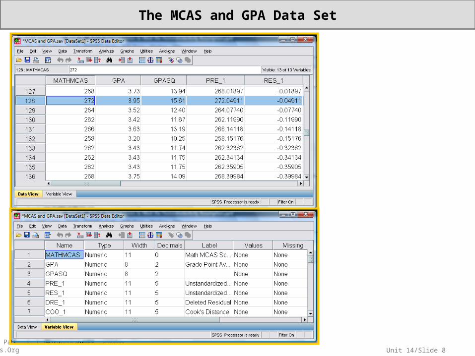
Data Set: MCAS and GPA (MCAS and GPA.sav): Math MCAS scaled scores and GPAs for the 223 sophomores at an anonymous Massachusetts high school (AHS), date withheld.
Variables: Outcome—Math MCAS Scaled Score (MATHMCAS) Predictor—Sophomore Grade Point Average (GPA)
Using Tukey’s Rule of the Bulge, should we try going up in X, down in X, up in Y or down in Y? Pick two. Of the two, which is the better as suggested by the histograms?
I had SPSS drop a quadratic trend line instead of a mean line in order to guide my eye. There is a slight horseshoe. Note that in an RVF plot, there should be no pattern. The trend line and mean line should be identical.
Unit 14/Slide 11
Exploratory Graphs (Second Iteration)
Again, I had SPSS drop a quadratic curve to guide my eye. You can see a slight curvature but it’s linear enough for government work.
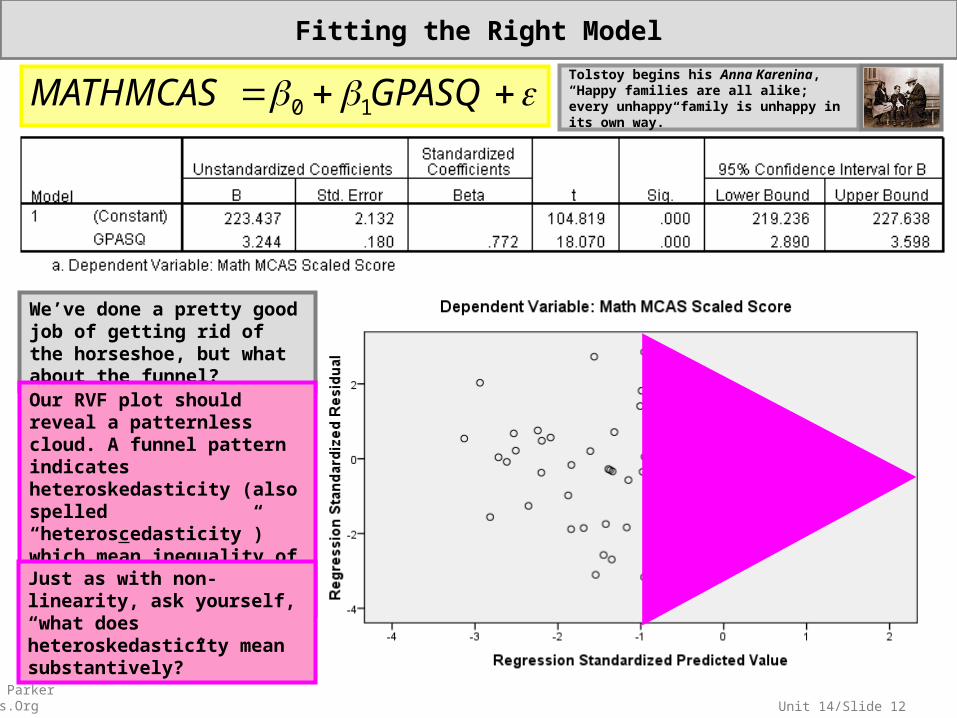
We’ve done a pretty good job of getting rid of the horseshoe, but what about the funnel?Our RVF plot should reveal a patternless cloud. A funnel pattern indicates heteroskedasticity (also spelled “heteroscedasticity”) which mean inequality of variances conditional on X. Just as with non-linearity, ask yourself, “what does heteroskedasticity mean substantively?”
Tolstoy begins his Anna Karenina, “Happy families are all alike; every unhappy family is unhappy in its own way.”
The problem with heteroskedasticity is not in our parameter estimates: the intercept and slope coefficients will be unbiased, because they are conditional averages, and conditional averages do not care about conditional variances. The problem is in our standard errors. Recall that a standard error is just a special kind of standard deviation—the standard deviation of THE sampling distribution. But, when there is a different sampling distribution at each level of X, which do we choose?A solution is to calculate robust standard errors by using heteroskedasticity-consistent (HC) estimators.
Sadly, SPSS offers no easy way to implement heteroskedasticity-consistent standard error (HCSE) estimation. In addition to a relatively comprehensible discussion of HCSE, Hayes and Cai (2007) provide two pages of SPSS syntax for HCSE: http://www.comm.ohio-state.edu/ahayes/BRM2007.pdf. Other statistical packages, however, have built-in HCSE functionality, so we will switch to one–Stata.Roughly speaking, psychologists use SPSS, economists use Stata, and statisticians use SAS or R. Each package has its strengths and weaknesses, although you will find zealots for each who will disagree.
2
1
6
4
3
5
1. File
2. Save As…
3. Scroll down files types until you find your version of Stata (or something close).
4. Choose your version of Stata (or something close).
Through your MS Windows “Programs” menu, open your version of Stata. From Stata, open (File > Open…) your Stata formatted data set (*.dta). In the command window, enter your syntax, then hit enter.
If you want to copy and paste your output into a Word document, highlight and copy as normal. When you paste, you’ll find that the format is screwy. Change the font to Courier (a monospace-type font), and things should line up.
Since there is no easy way to copy and paste the output into a Word document, copy the entire screen by hitting both your function key and your print screen key simultaneously. The screen shot is now on your clipboard ready for pasting.
Unit 14/Slide 17
Comparing our Stata Output with our SPSS Output
SPSS Outpu
t
Stata Outpu
t
Same Different
Do not memorize this, but be able to think in these terms based on your deepening understanding of standard errors:
Figure 13.a. A fitted regression line showing the relationship between GPA and predicted math MCAS scaled scores for 223 AHS sophomores.
In our sample of 223 sophomores attending AHS, we found a statistically significant non-linear positive relationship between MATHMCAS and GPA2, t(221) = 16.36, p < .001. We used robust standard errors (HC3) to derive our t statistic in order to correct for the heteroskedasticity in the data. Students with lower GPAs tended to exhibit greater variation in math MCAS scores than students with higher GPAs. We squared our predictor, GPA, in order to linearize the relationship for the purposes of OLS regression. Small differences among high GPAs lead us to predict fairly large differences in math MCAS scores, whereas small differences among low GPAs lead us to predict only small differences in math MCAS scores. Take for instance two students with A- and A overall GPAs, respectively. Based on averages, we predict that the higher GPA student will score more than 7 MCAS points higher. However, if we take two students with D- and D overall GPAs, respectively, we predict that the higher GPA student will score less than 2 MCAS points higher. Based on this trend, we can make controlled observations of students, identifying students who outperform or underperform our predictions, so that we can learn from their educational strategies in order to improve our educational strategies.
Sometimes heteroskedasticity appears because we are specifying the wrong model. Sometimes the cure for heteroskedasticity is multiple regression with interactions, which we learn in Unit 17.Imagine that we examine the relationship between MCAS and GPA for girls and boys separately. It is possible that two (or more) homoskedastic relationships can be heteroskedastic when taken as a whole.
Note that the sex variable is fictitious for the sake of illustration.
If we can model the pattern of heteroskedasticity in terms of the predictors, we can do weighted least squares (WLS) regression instead of ordinary least squares (OLS) regression. This WLS solution is very difficult, because it requires a theory of population variation so specific that we can mathematize it. However, if we have the right theory and the right formula for that theory, we can weight our observations appropriately and derive standard errors from a weighted average sampling distribution.
Other Solutions: Statistical Interaction and Weighted Least Squares
Underlying most statistical tests are mathematical proofs that you could learn to comprehend in a theoretical statistics course. At Harvard, the prerequisites for Statistics 101 are three courses in calculus (differentiation, integration, and multivariable), a course in linear algebra and a course in probability. Note that heteroskedasticity-consistent standard errors are too advanced for Statistics 101.
White’s (1980) article on HCSEs is the most cited article in economics since being published. He invented (or is it “discovered”?) HC0 estimators which were improved upon by other statisticians who found HC0 estimators were not robust in small samples, and they invented/discovered HC3 estimators to solve the small sample problem.
White; Halbert (1980), "A Heteroskedasticity-Consistent Covariance Matrix Estimator and a Direct Test for Heteroskedasticity", Econometrica 48 (4): 817--838, doi:10.2307/1912934
truttruthh
• The statisticians tell me that the HCSE math works. (I am working on the skills to check myelf.)
• The Monte Carlo methodologists can’t come up with a heteroskedastic population in which HCSEs fail. (Again, I am working on the skills to try my hand at creating a problematic population.)
• The economists have adopted HCSEs nearly unanimously. (A million economists can’t be wrong, right? Right?)
Monte Carlo methods provide statistical tests for statistical tests. A statistical test can justify our inference from a sample to a population, but what justifies our reliance on the statistical test? Underlying most statistical tests are mathematical proofs that you could learn to comprehend in a theoretical statistics course. However, in the meantime, there are more comprehensible methods for support. A statistical programmer can create her own population (with carefully specified parameters) and draw a random sample from it. She can then use a statistical test to draw conclusions from the sample to the population, but because she created the population, she already knows the right answer, so she can determine whether the test is working as advertised. These methods are called Monte Carlo methods after the famous casino city of Monte Carlo.
We can do our own Monte Carlo test of non-robust standard errors. We can specify a population in which there is no average difference between boys and girls, but in which there is a difference in variances (e.g., heteroskedasticity). Our Type I Error Rate should be 0.05 because our alpha level is 0.05. Is our Type I Error Rate in fact 0.05?
All GLM-based statistical tests are fairly robust to small violations of the homoskedasticity (and normality) assumptions.
Unit 14/Slide 24
We Can Calculate “Robust” Standard Errors for Two-Sample T-Tests
A two-sample T-test is just the T-test for the slope coefficient from regressing a continuous outcome on a dichotomous predictor. Because they are so easy to calculate by hand, two-sample T-tests are the focus of many statistics courses which use them to introduce the concept of statistical hypothesis testing. (I don’t focus on two-sample T-tests, because I focus on the more general tool of regression which subsumes two-sample T-tests.)
A Translation Guide
Two-Sample T-Test Language Regression Language
Two Populations One sample from one population, with two groups indicated by a dichotomous predictor variable
Two Samples
Estimated Mean Difference Slope Parameter Estimate (β1)
The key to any statistical null-hypothesis test is to see if your estimate is more than two standard errors from zero. Thus, the key is calculating standard errors, by which you can divide your estimate.“Non-Robust” Standard Error (i.e.,
As we can see from this RVF plot, there is a ceiling effect, which is easy to mistake for heteroskedasticity. If we look closely at the slices, however, we see that their variances are roughly equal. We’ll try robust standard errors anyway, but no data analytic decision is going to undo the ceiling effect. In the words of John Willett, “We cannot fix with data analysis what we bungled by design.”
Unit 14: How do we deal with violations of the heteroskedasticity assumptions?
Our RVF plot should reveal a patternless cloud. A funnel pattern indicates heteroskedasticity (also spelled “heteroscedasticity”) which mean inequality of variances conditional on X.
Just as with non-linearity, ask yourself, “what does heteroskedasticity mean substantively?”
The problem with heteroskedasticity is not in our parameter estimates: the intercept and slope coefficients will be unbiased, because they are conditional averages, and conditional averages do not care about conditional variances.
A solution is to calculate robust standard errors by using heteroskedasticity-consistent (HC) estimators.
The problem is in our standard errors. Recall that a standard error is just a special kind of standard deviation—the standard deviation of THE sampling distribution. But, when there is a different sampling distribution at each level of X, which do we choose?
Do not memorize this, but be able to think in these terms based on your deepening understanding of standard errors: When we use HC standard errors, sometimes, as is the case here, they will be smaller than our run of the mill standard errors, but other times they will be larger. One way or the other, HC standard error are more trustworthy when we are analyzing heteroskedastic relationships. In terms of statistical significance, when our standard errors are too small (as is the case with our SPSS output), we are too prone to Type I Error (i.e., mistakenly rejecting the null hypothesis). When our standard errors are too large we are too prone to Type II Error (i.e., mistakenly failing to reject the null hypothesis). In terms of confidence intervals, when our standard errors are too small as is the case with or SPSS output, our 95% confidence intervals are really less than 95%. When our standard errors are too large, our 95% confidence intervals are really more than 95%.
Sometimes heteroskedasticity appears because we are specifying the wrong model. Sometimes the cure for heteroskedasticity is multiple regression with interactions, which we learn in Unit 17.
All GLM-based statistical tests are fairly robust to small violations of the homoskedasticity (and normality) assumptions.
In our sample of 223 sophomores attending AHS, we found a statistically significant non-linear positive relationship between MATHMCAS and GPA2, t(221) = 16.36, p < .001. We used robust standard errors (HC3) to derive our t statistic in order to correct for the heteroskedasticity in the data. Students with lower GPAs tended to exhibit greater variation in math MCAS scores than students with higher GPAs. We squared our predictor, GPA, in order to linearize the relationship for the purposes of OLS regression. Small differences among high GPAs lead us to predict fairly large differences in math MCAS scores, whereas small differences among low GPAs lead us to predict only small differences in math MCAS scores. Take for instance two students with A- and A overall GPAs, respectively. Based on averages, we predict that the higher GPA student will score more than 7 MCAS points higher. However, if we take two students with D- and D overall GPAs, respectively, we predict that the higher GPA student will score less than 2 MCAS points higher. Based on this trend, we can make controlled observations of students, identifying students who outperform or underperform our predictions, so that we can learn from their educational strategies in order to improve our educational strategies.
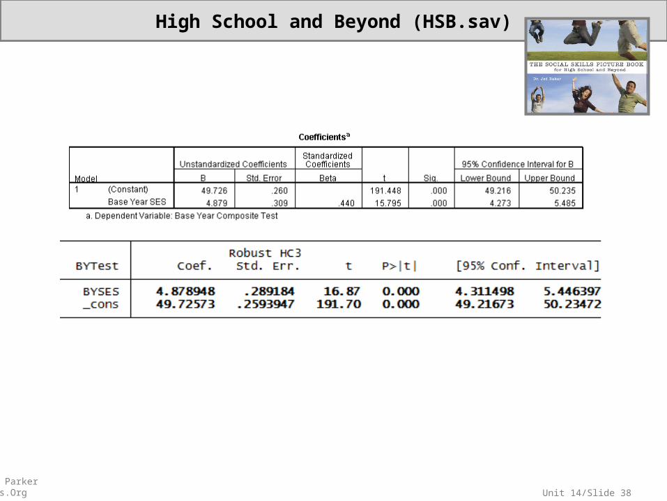
In order to address heteroskedasticity concerns, we used robust standard errors (HC3).
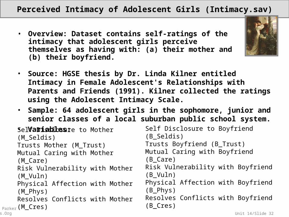
Perceived Intimacy of Adolescent Girls (Intimacy.sav)
• Source: HGSE thesis by Dr. Linda Kilner entitled Intimacy in Female Adolescent's Relationships with Parents and Friends (1991). Kilner collected the ratings using the Adolescent Intimacy Scale.
• Sample: 64 adolescent girls in the sophomore, junior and senior classes of a local suburban public school system.
• Variables:Self Disclosure to Mother (M_Seldis)Trusts Mother (M_Trust)Mutual Caring with Mother (M_Care)Risk Vulnerability with Mother (M_Vuln)Physical Affection with Mother (M_Phys)Resolves Conflicts with Mother (M_Cres)
Self Disclosure to Boyfriend (B_Seldis)Trusts Boyfriend (B_Trust)Mutual Caring with Boyfriend (B_Care)Risk Vulnerability with Boyfriend (B_Vuln)Physical Affection with Boyfriend (B_Phys)Resolves Conflicts with Boyfriend (B_Cres)
• Overview: Dataset contains self-ratings of the intimacy that adolescent girls perceive themselves as having with: (a) their mother and (b) their boyfriend.
• Source: Subset of data graciously provided by Valerie Lee, University of Michigan.
• Sample: This subsample has 1044 students in 205 schools. Missing data on the outcome test score and family SES were eliminated. In addition, schools with fewer than 3 students included in this subset of data were excluded.
• Variables:
Variables about the student—
(Black) 1=Black, 0=Other(Latin) 1=Latino/a, 0=Other(Sex) 1=Female, 0=Male(BYSES) Base year SES (GPA80) HS GPA in 1980 (GPS82) HS GPA in 1982(BYTest) Base year composite of reading and math tests(BBConc) Base year self concept(FEConc) First Follow-up self concept
Variables about the student’s school—
(PctMin) % HS that is minority students Percentage(HSSize) HS Size (PctDrop) % dropouts in HS Percentage(BYSES_S) Average SES in HS sample(GPA80_S) Average GPA80 in HS sample(GPA82_S) Average GPA82 in HS sample(BYTest_S) Average test score in HS sample(BBConc_S) Average base year self concept in HS sample(FEConc_S) Average follow-up self concept in HS sample
• Overview: High School & Beyond – Subset of data focused on selected student and school characteristics as predictors of academic achievement.
• Source: Perrin E.C., Sayer A.G., and Willett J.B. (1991). Sticks And Stones May Break My Bones: Reasoning About Illness Causality And Body Functioning In Children Who Have A Chronic Illness, Pediatrics, 88(3), 608-19.
• Sample: 301 children, including a sub-sample of 205 who were described as asthmatic, diabetic,or healthy. After further reductions due to the list-wise deletion of cases with missing data on one or more variables, the analytic sub-sample used in class ends up containing: 33 diabetic children, 68 asthmatic children and 93 healthy children.
• Variables:(ILLCAUSE) Child’s Understanding of Illness Causality (SES) Child’s SES (Note that a high score means low SES.)(PPVT) Child’s Score on the Peabody Picture Vocabulary Test(AGE) Child’s Age, In Months(GENREAS) Child’s Score on a General Reasoning Test(ChronicallyIll) 1 = Asthmatic or Diabetic, 0 = Healthy(Asthmatic) 1 = Asthmatic, 0 = Healthy(Diabetic) 1 = Diabetic, 0 = Healthy
• Overview: Data for investigating differences in children’s understanding of the causes of illness, by their health status.
• Source: Portes, Alejandro, & Ruben G. Rumbaut (2001). Legacies: The Story of the Immigrant SecondGeneration. Berkeley CA: University of California Press.
• Sample: Random sample of 880 participants obtained through the website.• Variables:
(Reading) Stanford Reading Achievement Score(Freelunch) % students in school who are eligible for free lunch program(Male) 1=Male 0=Female(Depress) Depression scale (Higher score means more depressed)(SES) Composite family SES score
• Overview: “CILS is a longitudinal study designed to study the adaptation process of the immigrant second generation which is defined broadly as U.S.-born children with at least one foreign-born parent or children born abroad but brought at an early age to the United States. The original survey was conducted with large samples of second-generation children attending the 8th and 9th grades in public and private schools in the metropolitan areas of Miami/Ft. Lauderdale in Florida and San Diego, California” (from the website description of the data set).
Human Development in Chicago Neighborhoods (Neighborhoods.sav)
• Source: Sampson, R.J., Raudenbush, S.W., & Earls, F. (1997). Neighborhoods and violent crime: A multilevel study of collective efficacy. Science, 277, 918-924.
• Sample: The data described here consist of information from 343 Neighborhood Clusters in Chicago Illinois. Some of the variables were obtained by project staff from the 1990 Census and city records. Other variables were obtained through questionnaire interviews with 8782 Chicago residents who were interviewed in their homes.
• Variables:
(Homr90) Homicide Rate c. 1990(Murder95) Homicide Rate 1995(Disadvan) Concentrated Disadvantage (Imm_Conc) Immigrant (ResStab) Residential Stability (Popul) Population in 1000s(CollEff) Collective Efficacy(Victim) % Respondents Who Were Victims of Violence(PercViol) % Respondents Who Perceived Violence
• These data were collected as part of the Project on Human Development in Chicago Neighborhoods in 1995.
• Sample: These data consist of seventh graders who participated in Wave 3 of the 4-H Study of Positive Youth Development at Tufts University. This subfile is a substantially sampled-down version of the original file, as all the cases with any missing data on these selected variables were eliminated.
• Variables:
(SexFem) 1=Female, 0=Male(MothEd) Years of Mother’s Education(Grades) Self-Reported Grades (Depression) Depression (Continuous)(FrInfl) Friends’ Positive Influences (PeerSupp) Peer Support (Depressed) 0 = (1-15 on Depression) 1 = Yes (16+ on Depression)
• 4-H Study of Positive Youth Development• Source: Subset of data from IARYD, Tufts