63
Unit 2: Probability and distributions 3. Normal and binomial distributions GOVT 3990 - Spring 2020 Cornell University

Unit 2: Probability and distributions
3. Normal and binomial distributions
GOVT 3990 - Spring 2020
Cornell University
Dr. Garcia-Rios Slides posted at http://garciarios.github.io/govt 3990/
Outline
1. Housekeeping
2. Main ideas
1. Two types of probability distributions: discrete and continuous
2. Normal distribution is unimodal, symmetric, and follows the 68-95-99.7
rule
3. Z scores serve as a ruler for any distribution
4. Binomial distribution is used for calculating the probability of exact
number of successes for a given number of trials
5. Expected value and standard deviation of the binomial can be
calculated using its parameters n and p
6. Shape of the binomial distribution approaches normal when the S-F rule
is met
3. Summary

Announcements
I Labs:
– what you did right
– what you did wrong
– Lab 1 graded, lab 2 this weekend
– Lab 3 Due next week
1

Announcements
I Labs:
– what you did right
– what you did wrong
– Lab 1 graded, lab 2 this weekend
– Lab 3 Due next week
1
Announcements
I Labs:
– what you did right
– what you did wrong
– Lab 1 graded, lab 2 this weekend
– Lab 3 Due next week
1
Announcements
I Labs:
– what you did right
– what you did wrong
– Lab 1 graded, lab 2 this weekend
– Lab 3 Due next week
1

Outline
1. Housekeeping
2. Main ideas
1. Two types of probability distributions: discrete and continuous
2. Normal distribution is unimodal, symmetric, and follows the 68-95-99.7
rule
3. Z scores serve as a ruler for any distribution
4. Binomial distribution is used for calculating the probability of exact
number of successes for a given number of trials
5. Expected value and standard deviation of the binomial can be
calculated using its parameters n and p
6. Shape of the binomial distribution approaches normal when the S-F rule
is met
3. Summary
1. Two types of probability distributions: discrete and continuous
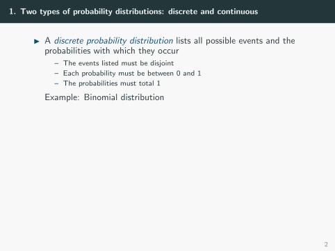
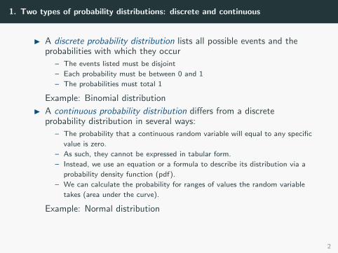
I A discrete probability distribution lists all possible events and theprobabilities with which they occur
– The events listed must be disjoint
– Each probability must be between 0 and 1
– The probabilities must total 1
Example: Binomial distribution
I A continuous probability distribution differs from a discreteprobability distribution in several ways:
– The probability that a continuous random variable will equal to any specific
value is zero.
– As such, they cannot be expressed in tabular form.
– Instead, we use an equation or a formula to describe its distribution via a
probability density function (pdf).
– We can calculate the probability for ranges of values the random variable
takes (area under the curve).
Example: Normal distribution
2
1. Two types of probability distributions: discrete and continuous
I A discrete probability distribution lists all possible events and theprobabilities with which they occur
– The events listed must be disjoint
– Each probability must be between 0 and 1
– The probabilities must total 1
Example: Binomial distribution
I A continuous probability distribution differs from a discreteprobability distribution in several ways:
– The probability that a continuous random variable will equal to any specific
value is zero.
– As such, they cannot be expressed in tabular form.
– Instead, we use an equation or a formula to describe its distribution via a
probability density function (pdf).
– We can calculate the probability for ranges of values the random variable
takes (area under the curve).
Example: Normal distribution
2
Outline
1. Housekeeping
2. Main ideas
1. Two types of probability distributions: discrete and continuous
2. Normal distribution is unimodal, symmetric, and follows the 68-95-99.7
rule
3. Z scores serve as a ruler for any distribution
4. Binomial distribution is used for calculating the probability of exact
number of successes for a given number of trials
5. Expected value and standard deviation of the binomial can be
calculated using its parameters n and p
6. Shape of the binomial distribution approaches normal when the S-F rule
is met
3. Summary
Your turn
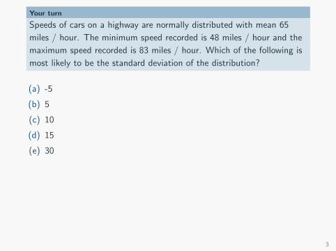
Speeds of cars on a highway are normally distributed with mean 65
miles / hour. The minimum speed recorded is 48 miles / hour and the
maximum speed recorded is 83 miles / hour. Which of the following is
most likely to be the standard deviation of the distribution?
(a) -5
(b) 5
(c) 10
(d) 15
(e) 30
3

Your turn
Speeds of cars on a highway are normally distributed with mean 65
miles / hour. The minimum speed recorded is 48 miles / hour and the
maximum speed recorded is 83 miles / hour. Which of the following is
most likely to be the standard deviation of the distribution?
(a) -5 → SD cannot be negative
(b) 5 → 65± (3× 5) = (50, 80)
(c) 10 → 65± (3× 10) = (35, 95)
(d) 15 → 65± (3× 15) = (20, 110)
(e) 30 → 65± (3× 30) = (−25, 155)
3

Outline
1. Housekeeping
2. Main ideas
1. Two types of probability distributions: discrete and continuous
2. Normal distribution is unimodal, symmetric, and follows the 68-95-99.7
rule
3. Z scores serve as a ruler for any distribution
4. Binomial distribution is used for calculating the probability of exact
number of successes for a given number of trials
5. Expected value and standard deviation of the binomial can be
calculated using its parameters n and p
6. Shape of the binomial distribution approaches normal when the S-F rule
is met
3. Summary
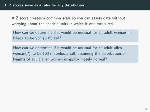
3. Z scores serve as a ruler for any distribution
A Z score creates a common scale so you can assess data without
worrying about the specific units in which it was measured.
How can we determine if it would be unusual for an adult woman in
Ithaca to be 96” (8 ft) tall?
How can we determine if it would be unusual for an adult alien
woman(?) to be 103 metreloots tall, assuming the distribution of
heights of adult alien women is approximately normal?
4

3. Z scores serve as a ruler for any distribution
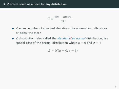
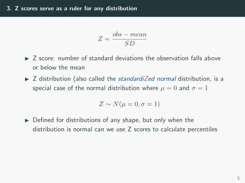
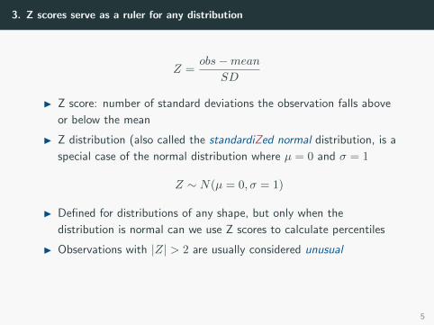
Z =obs−mean
SD
I Z score: number of standard deviations the observation falls above
or below the mean
I Z distribution (also called the standardiZed normal distribution, is a
special case of the normal distribution where µ = 0 and σ = 1
Z ∼ N(µ = 0, σ = 1)
I Defined for distributions of any shape, but only when the
distribution is normal can we use Z scores to calculate percentiles
I Observations with |Z| > 2 are usually considered unusual
5
3. Z scores serve as a ruler for any distribution
Z =obs−mean
SD
I Z score: number of standard deviations the observation falls above
or below the mean
I Z distribution (also called the standardiZed normal distribution, is a
special case of the normal distribution where µ = 0 and σ = 1
Z ∼ N(µ = 0, σ = 1)
I Defined for distributions of any shape, but only when the
distribution is normal can we use Z scores to calculate percentiles
I Observations with |Z| > 2 are usually considered unusual
5

Your turn
Scores on a standardized test are normally distributed with a mean of
100 and a standard deviation of 20. If these scores are converted to
standard normal Z scores, which of the following statements will be
correct?
(a) The mean will equal 0, but the median cannot be determined.
(b) The mean of the standardized Z-scores will equal 100.
(c) The mean of the standardized Z-scores will equal 5.
(d) Both the mean and median score will equal 0.
(e) A score of 70 is considered unusually low on this test.
6
Outline
1. Housekeeping
2. Main ideas
1. Two types of probability distributions: discrete and continuous
2. Normal distribution is unimodal, symmetric, and follows the 68-95-99.7
rule
3. Z scores serve as a ruler for any distribution
4. Binomial distribution is used for calculating the probability of exact
number of successes for a given number of trials
5. Expected value and standard deviation of the binomial can be
calculated using its parameters n and p
6. Shape of the binomial distribution approaches normal when the S-F rule
is met
3. Summary

High-speed broadband connection at home in the US
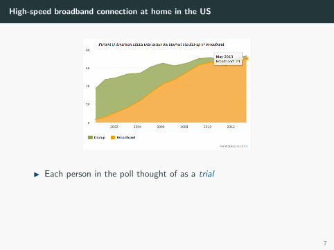
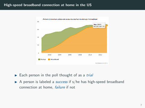
I Each person in the poll thought of as a trial
I A person is labeled a success if s/he has high-speed broadband
connection at home, failure if not
I Since 70% have high-speed broadband connection at home,
probability of success is p = 0.70
7
High-speed broadband connection at home in the US
I Each person in the poll thought of as a trial
I A person is labeled a success if s/he has high-speed broadband
connection at home, failure if not
I Since 70% have high-speed broadband connection at home,
probability of success is p = 0.70
7
High-speed broadband connection at home in the US
I Each person in the poll thought of as a trial
I A person is labeled a success if s/he has high-speed broadband
connection at home, failure if not
I Since 70% have high-speed broadband connection at home,
probability of success is p = 0.70
7

High-speed broadband connection at home in the US
I Each person in the poll thought of as a trial
I A person is labeled a success if s/he has high-speed broadband
connection at home, failure if not
I Since 70% have high-speed broadband connection at home,
probability of success is p = 0.70
7
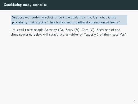
Considering many scenarios
Suppose we randomly select three individuals from the US, what is the
probability that exactly 1 has high-speed broadband connection at home?
Let’s call these people Anthony (A), Barry (B), Cam (C). Each one of the
three scenarios below will satisfy the condition of “exactly 1 of them says Yes”:
Scenario 1:0.70
(A) yes× 0.30
(B) no× 0.30
(C) no≈ 0.063
Scenario 2:0.30
(A) no× 0.70
(B) yes× 0.30
(C) no≈ 0.063
Scenario 3:0.30
(A) no× 0.30
(B) no× 0.70
(C) yes≈ 0.063
The probability of exactly one 1 of 3 people saying Yes is the sum of all of
these probabilities.
0.063 + 0.063 + 0.063 = 3× 0.063 = 0.189
8
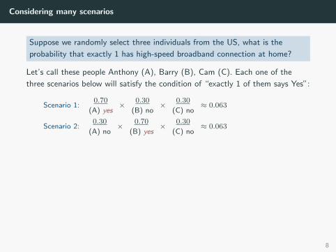
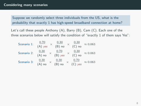

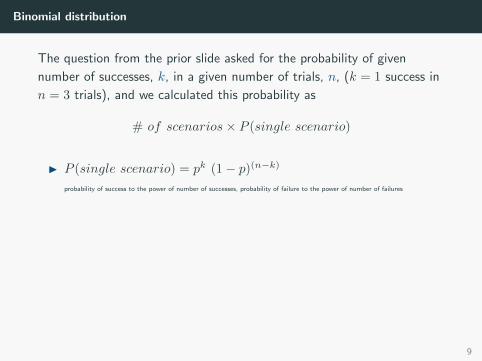
Binomial distribution
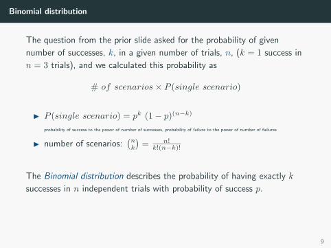
The question from the prior slide asked for the probability of given
number of successes, k, in a given number of trials, n, (k = 1 success in
n = 3 trials), and we calculated this probability as
# of scenarios× P (single scenario)
I P (single scenario) = pk (1− p)(n−k)
probability of success to the power of number of successes, probability of failure to the power of number of failures
I number of scenarios:(nk
)= n!
k!(n−k)!
The Binomial distribution describes the probability of having exactly k
successes in n independent trials with probability of success p.
9
Binomial distribution
The question from the prior slide asked for the probability of given
number of successes, k, in a given number of trials, n, (k = 1 success in
n = 3 trials), and we calculated this probability as
# of scenarios× P (single scenario)
I P (single scenario) = pk (1− p)(n−k)
probability of success to the power of number of successes, probability of failure to the power of number of failures
I number of scenarios:(nk
)= n!
k!(n−k)!
The Binomial distribution describes the probability of having exactly k
successes in n independent trials with probability of success p.
9

Binomial distribution (cont.)
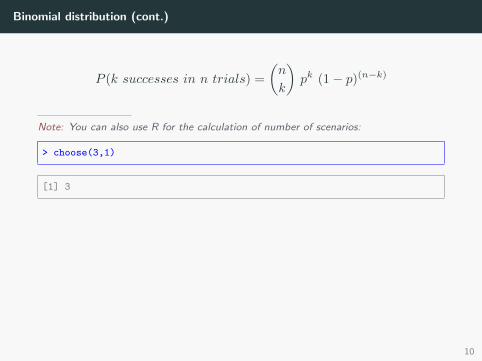
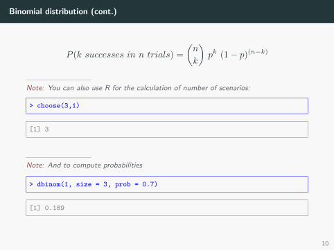
P (k successes in n trials) =
(n
k
)pk (1− p)(n−k)
Note: You can also use R for the calculation of number of scenarios:
> choose(3,1)
[1] 3
Note: And to compute probabilities
> dbinom(1, size = 3, prob = 0.7)
[1] 0.189
10
Binomial distribution (cont.)
P (k successes in n trials) =
(n
k
)pk (1− p)(n−k)
Note: You can also use R for the calculation of number of scenarios:
> choose(3,1)
[1] 3
Note: And to compute probabilities
> dbinom(1, size = 3, prob = 0.7)
[1] 0.189
10
Binomial distribution (cont.)
P (k successes in n trials) =
(n
k
)pk (1− p)(n−k)
Note: You can also use R for the calculation of number of scenarios:
> choose(3,1)
[1] 3
Note: And to compute probabilities
> dbinom(1, size = 3, prob = 0.7)
[1] 0.189
10

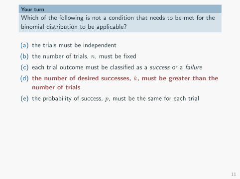
Your turn
Which of the following is not a condition that needs to be met for the
binomial distribution to be applicable?
(a) the trials must be independent
(b) the number of trials, n, must be fixed
(c) each trial outcome must be classified as a success or a failure
(d) the number of desired successes, k, must be greater than the
number of trials
(e) the probability of success, p, must be the same for each trial
11
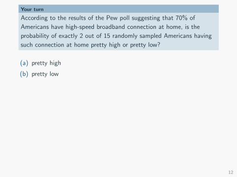
Your turn
According to the results of the Pew poll suggesting that 70% of
Americans have high-speed broadband connection at home, is the
probability of exactly 2 out of 15 randomly sampled Americans having
such connection at home pretty high or pretty low?
(a) pretty high
(b) pretty low
12
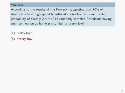
Your turn
According to the results of the Pew poll suggesting that 70% of
Americans have high-speed broadband connection at home, is the
probability of exactly 2 out of 15 randomly sampled Americans having
such connection at home pretty high or pretty low?
(a) pretty high
(b) pretty low
12
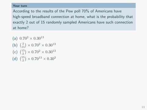
Your turn
According to the results of the Pew poll 70% of Americans have
high-speed broadband connection at home, what is the probability that
exactly 2 out of 15 randomly sampled Americans have such connection
at home?
(a) 0.702 × 0.3013
(b)(215
)× 0.702 × 0.3013
(c)(152
)× 0.702 × 0.3013
(d)(152
)× 0.7013 × 0.302
13

Your turn
According to the results of the Pew poll 70% of Americans have
high-speed broadband connection at home, what is the probability that
exactly 2 out of 15 randomly sampled Americans have such connection
at home?
(a) 0.702 × 0.3013
(b)(215
)× 0.702 × 0.3013
(c)(152
)× 0.702 × 0.3013
= 15!13!×2! × 0.702 × 0.3013 = 105× 0.702 × 0.3013 = 8.2e− 06
(d)(152
)× 0.7013 × 0.302
13
Outline
1. Housekeeping
2. Main ideas
1. Two types of probability distributions: discrete and continuous
2. Normal distribution is unimodal, symmetric, and follows the 68-95-99.7
rule
3. Z scores serve as a ruler for any distribution
4. Binomial distribution is used for calculating the probability of exact
number of successes for a given number of trials
5. Expected value and standard deviation of the binomial can be
calculated using its parameters n and p
6. Shape of the binomial distribution approaches normal when the S-F rule
is met
3. Summary
Expected value and standard deviation of binomial
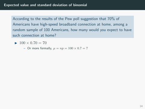
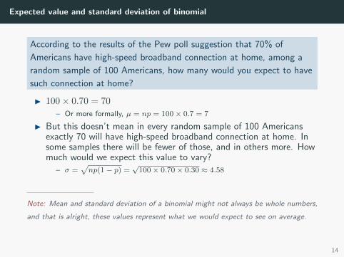
According to the results of the Pew poll suggestion that 70% of
Americans have high-speed broadband connection at home, among a
random sample of 100 Americans, how many would you expect to have
such connection at home?
I 100× 0.70 = 70
– Or more formally, µ = np = 100× 0.7 = 7
I But this doesn’t mean in every random sample of 100 Americansexactly 70 will have high-speed broadband connection at home. Insome samples there will be fewer of those, and in others more. Howmuch would we expect this value to vary?
– σ =√np(1− p) =
√100× 0.70× 0.30 ≈ 4.58
Note: Mean and standard deviation of a binomial might not always be whole numbers,
and that is alright, these values represent what we would expect to see on average.
14

Expected value and standard deviation of binomial
According to the results of the Pew poll suggestion that 70% of
Americans have high-speed broadband connection at home, among a
random sample of 100 Americans, how many would you expect to have
such connection at home?
I 100× 0.70 = 70
– Or more formally, µ = np = 100× 0.7 = 7
I But this doesn’t mean in every random sample of 100 Americansexactly 70 will have high-speed broadband connection at home. Insome samples there will be fewer of those, and in others more. Howmuch would we expect this value to vary?
– σ =√np(1− p) =
√100× 0.70× 0.30 ≈ 4.58
Note: Mean and standard deviation of a binomial might not always be whole numbers,
and that is alright, these values represent what we would expect to see on average.
14

Outline
1. Housekeeping
2. Main ideas
1. Two types of probability distributions: discrete and continuous
2. Normal distribution is unimodal, symmetric, and follows the 68-95-99.7
rule
3. Z scores serve as a ruler for any distribution
4. Binomial distribution is used for calculating the probability of exact
number of successes for a given number of trials
5. Expected value and standard deviation of the binomial can be
calculated using its parameters n and p
6. Shape of the binomial distribution approaches normal when the S-F rule
is met
3. Summary

Shape of the binomial distribution
https://gallery.shinyapps.io/dist calc/
You can use the normal distribution to approximate binomial probabilities
when the sample size is large enough.
S-F rule: The sample size is considered large enough if the expected
number of successes and failures are both at least 10
np ≥ 10 and n(1− p) ≥ 10
15
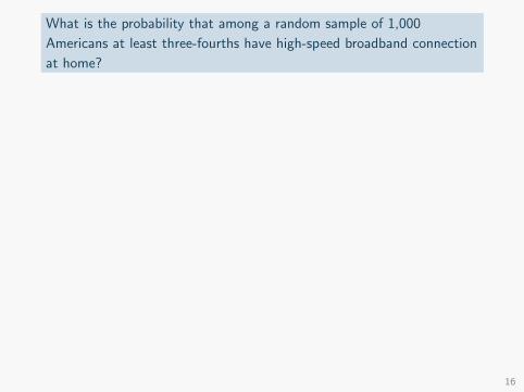
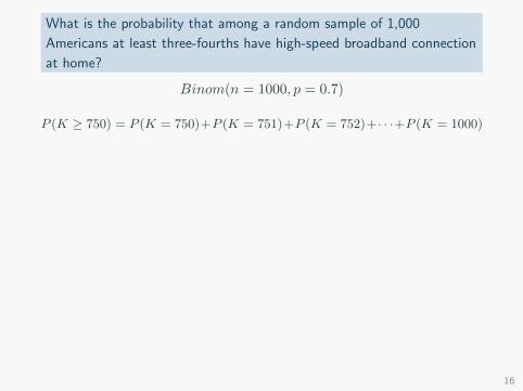
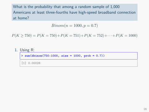
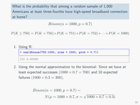
What is the probability that among a random sample of 1,000
Americans at least three-fourths have high-speed broadband connection
at home?
Binom(n = 1000, p = 0.7)
P (K ≥ 750) = P (K = 750)+P (K = 751)+P (K = 752)+· · ·+P (K = 1000)
1. Using R:
> sum(dbinom(750:1000, size = 1000, prob = 0.7))
[1] 0.00026
2. Using the normal approximation to the binomial: Since we have at
least expected successes (1000× 0.7 = 700) and 10 expected
failures (1000× 0.3 = 300),
Binom(n = 1000, p = 0.7) ∼N(µ = 1000× 0.7, σ =
√1000× 0.7× 0.3)
16

Outline
1. Housekeeping
2. Main ideas
1. Two types of probability distributions: discrete and continuous
2. Normal distribution is unimodal, symmetric, and follows the 68-95-99.7
rule
3. Z scores serve as a ruler for any distribution
4. Binomial distribution is used for calculating the probability of exact
number of successes for a given number of trials
5. Expected value and standard deviation of the binomial can be
calculated using its parameters n and p
6. Shape of the binomial distribution approaches normal when the S-F rule
is met
3. Summary

Summary of main ideas
1. Two types of probability distributions: discrete and continuous
2. Normal distribution is unimodal, symmetric, and follows the
68-95-99.7 rule
3. Z scores serve as a ruler for any distribution
4. Binomial distribution is used for calculating the probability of exact
number of successes for a given number of trials
5. Expected value and standard deviation of the binomial can be
calculated using its parameters n and p
6. Shape of the binomial distribution approaches normal when the S-F
rule is met
17


