32
Unit 3 Polynomials Mrs. Valen+ne Math III

Unit 3 PolynomialsMrs. Valen+ne
Math III

3.1 Dividing Polynomials• Long Division
– Numerical long division and polynomial long division are similar.
– Since the remainder of each is zero, 21 is a factor of 672 and 2x + 1 is a factor of 6x2 + 7x + 2.
– When dividing polynomials by long division, remainders are given the symbol R.
– Example: Divide 4x2 + 23x – 16 by x + 5.
Divide (9x2 – 21x – 20) by (x – 1)
63
3
42
2
42 0
3x
6x2 + 3x 4x + 2 4x + 2
+ 2
0
4x
4x2+ 20x 3x – 16 3x + 15
+ 3
– 31
R – 31
9x – 12, R – 32

3.1 Dividing Polynomials• Division Algorithm for Polynomials
– P(x) can be divided by D(x) to get polynomial quotient Q(x) and polynomial remainder R(x). The result is P(x) = D(x)Q(x) + R(x)
– If R(x) = 0, then D(x) and Q(x) are factors of P(x). – Example: is x2 + 1 a factor of 3x4 – 4x3 + 12x2 + 5?
Include 0x terms. 3x4 + 0x + 3x2
–4x3 + 9x2 + 0x –4x3 + 0x2 – 4x
9x2 + 4x + 5 9x2 + 0x + 9
4x – 4 Degree is less than divisor. Stop.
Remainder is not 0; x2 + 1 is not a factor of 3x4 – 4x3 + 12x2 + 5.
3x2 – 4x + 9

3.1 Dividing Polynomials• Synthetic Division (dividing by x – a)
– Write the coefficients (including zeros) of the polynomial in standard form.
– Omit all variables and exponents. – For the divisor, reverse the sign (use a), allowing addition instead of
subtraction. – Example: divide x3 – 14x2 + 51x – 54 by x + 2.
– Divide: (x3 – 3x2 – 5x – 25) ÷ (x – 5)
–2 1 –14 51 –54
1
• Bring down the first coefficient. • Mul+ply the coefficient by the divisor
and add to the next coefficient. • Quo+ent starts one degree below the
dividend.
–2 –16
32 83
–166 –220
Quo+ent is x2 – 16x + 83, R –220
5 1 –3 –5 –25
1 5
2 10 5
25 0
Quo+ent is x2 + 2x + 5

3.1 Dividing Polynomials• Applications
– The polynomial x3 + 7x2 – 38x – 240 expresses the volume, in cubic inches, of the shadow box shown. What are the dimensions of the box? (Reminder: length is always longest).
• Remainder Theorem – If you divide a polynomial P(x) of degree n ≥ 1 by x – a, then the
remainder is P(a). – Example: Given that P(x) = x5 – 2x3 – x2 + 2, what is P(3)?
3 1 0 –2 –1 0 2
1 3 3
9 7
21 20
60 60
180 182 P(3) = 182
Divide by x – 3
–5 1 7 –38 –240
1 –5 2
–10 –48 0
240
(x + 5)(x2 + 2x –48)
(x + 5)(x + 8)(x – 6)
(x2 + 2x –48) = (x + 8)(x – 6)
Length = (x + 8)in., width = (x + 5)in., height = (x – 6)in. (x + 5)

3.2 Theorems About the Roots of Polynomials• Rational Root Theorem
– Let P(x) = anxn + an–1xn–1 + … + a1x + a0 be a polynomial with integer coefficients. There are a limited number of possible roots of P(x) = 0:
• Integer roots must be factors of a0. • Rational roots: p/q , p = integer factor of a0 and q = integer factor of
an. • Descartes’s Rule of Signs
– Used to eliminate impossible roots quickly – The number of positive real roots = number of sign changes between
consecutive coefficients for P(x)=0 (or is less than that by an even number).
– The number of negative real roots = number of sign changes between consecutive coefficients for P(–x)=0 (or is less than that by an even number).
• Combined Example: What are the rational roots of 2x3 – x2 + 2x + 5 = 0?
2x3 – x2 + 2x + 5 = 0 2(–x)3 – (–x)2 + 2(–x) + 5 = 0 P(x)=0 P(–x)=0
(+) (–) (+) (+) (–) (–) (–) (+)
# Positive Roots: 2 or 0 # Negative Roots: 1
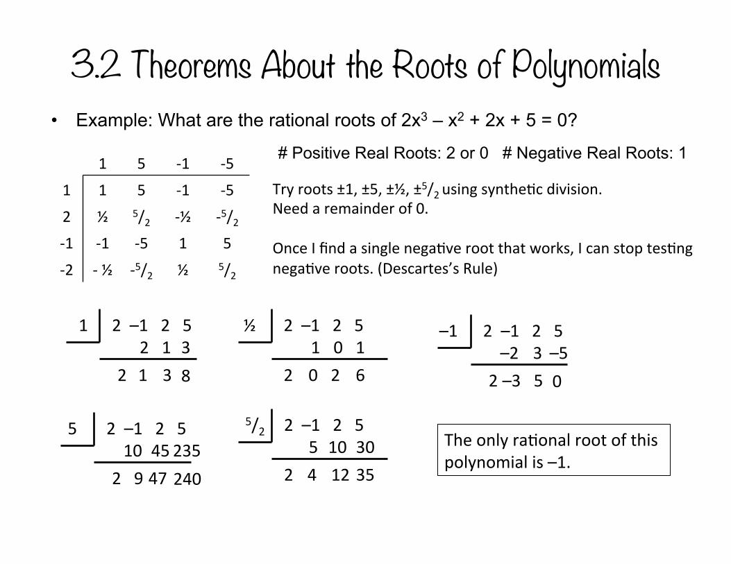
3.2 Theorems About the Roots of Polynomials• Example: What are the rational roots of 2x3 – x2 + 2x + 5 = 0?
1 5 -‐1 -‐5
1 1 5 -‐1 -‐5
2 ½ 5/2 -‐½ -‐5/2 -‐1 -‐1 -‐5 1 5
-‐2 -‐ ½ -‐5/2 ½ 5/2
Try roots ±1, ±5, ±½, ±5/2 using synthe+c division. Need a remainder of 0. Once I find a single nega+ve root that works, I can stop tes+ng nega+ve roots. (Descartes’s Rule)
1 2 –1 2 5
2 2 1
1 3 3 8
–1 2 –1 2 5
2 –2 –3
3 5
–5 0
5 2 –1 2 5
2 10 9
45 47
235 240
½ 2 –1 2 5
2 1 0
0 2
1 6
5/2 2 –1 2 5
2 5 4
10 12
30 35
The only ra+onal root of this polynomial is –1.
# Positive Real Roots: 2 or 0 # Negative Real Roots: 1

3.2 Theorems About the Roots of Polynomials• Imaginary Numbers
Ø i2 = –1 or i = √(–1). Ø a + bi is an imaginary number where a and b are real numbers and b ≠ 0. Ø Imaginary numbers and real numbers together are called complex numbers. Ø a + bi and a – bi are conjugates, as are a + √(b) and a – √(b).
• Conjugate Root Theorem – If P(x) is a polynomial with rational coefficients, then irrational roots of P(x) = 0
that have the form a + √(b) occur in conjugate pairs (a + √(b) is also a root) – If P(x) is a polynomial with real coefficients, then the complex roots of P(x) = 0
occur in conjugate pairs. (if a + bi is a root, then a – bi is also a root, where a and b are real).
– Example: A quartic polynomial P(x) has rational coefficients. If √(2) and 1 + i are roots of P(x) = 0, what are the two other roots?
0 + √(2)
0 – √(2)
–√(2)
1 + i
1 – i The other two roots are –√(2) and 1 – i
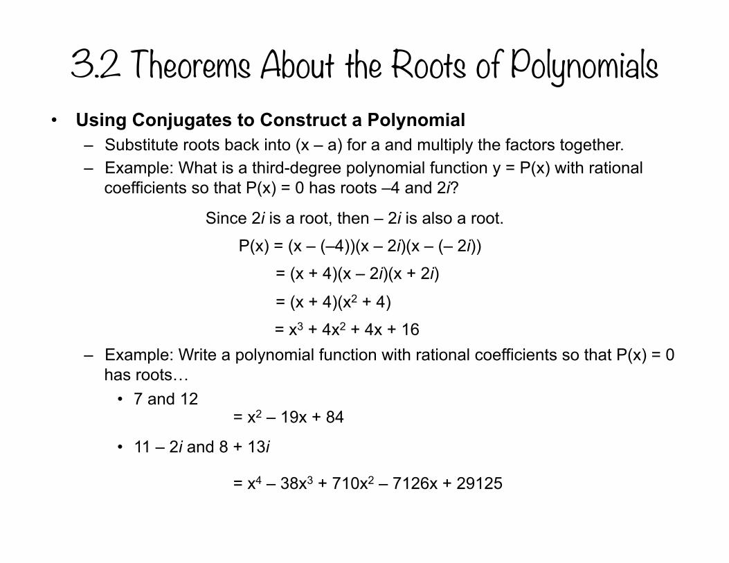
3.2 Theorems About the Roots of Polynomials• Using Conjugates to Construct a Polynomial
– Substitute roots back into (x – a) for a and multiply the factors together. – Example: What is a third-degree polynomial function y = P(x) with rational
coefficients so that P(x) = 0 has roots –4 and 2i?
– Example: Write a polynomial function with rational coefficients so that P(x) = 0 has roots…
• 7 and 12
• 11 – 2i and 8 + 13i
Since 2i is a root, then – 2i is also a root.
P(x) = (x – (–4))(x – 2i)(x – (– 2i))
= (x + 4)(x – 2i)(x + 2i)
= (x + 4)(x2 + 4)
= x3 + 4x2 + 4x + 16
= x2 – 19x + 84
= x4 – 38x3 + 710x2 – 7126x + 29125
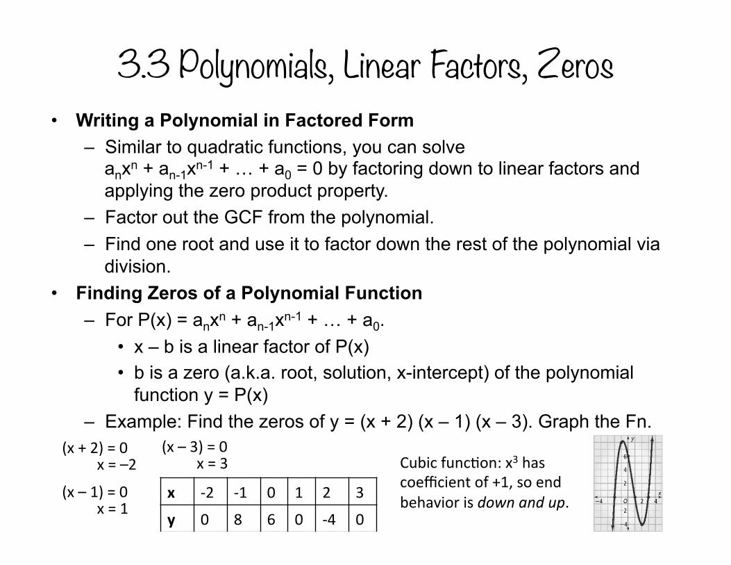
3.3 Polynomials, Linear Factors, Zeros• Writing a Polynomial in Factored Form
– Similar to quadratic functions, you can solve anxn + an-1xn-1 + … + a0 = 0 by factoring down to linear factors and applying the zero product property.
– Factor out the GCF from the polynomial. – Find one root and use it to factor down the rest of the polynomial via
division. • Finding Zeros of a Polynomial Function
– For P(x) = anxn + an-1xn-1 + … + a0. • x – b is a linear factor of P(x) • b is a zero (a.k.a. root, solution, x-intercept) of the polynomial
function y = P(x) – Example: Find the zeros of y = (x + 2) (x – 1) (x – 3). Graph the Fn.
(x + 2) = 0 x = –2
(x – 1) = 0 x = 1
(x – 3) = 0 x = 3
x -‐2 -‐1 0 1 2 3
y 0 8 6 0 -‐4 0
Cubic func+on: x3 has coefficient of +1, so end behavior is down and up.

3.3 Polynomials, Linear Factors, Zeros• Writing a Polynomial Function from its Zeros
– Use the zeros to write factors – Multiply the factors together (use the distributive property). – Example: What is a cubic function in standard form with zeros
–2, 2 and 3?
– Example: What is a quartic polynomial function in standard form with zeros -2, -2, 2, and 3?
f(x) = (x + 2) (x – 2) (x – 3)
f(x) = (x2 – 4) (x – 3)
f(x) = x3 – 3x2 – 4x + 12
f(x) = (x + 2) (x + 2) (x – 2) (x – 3)
f(x) = (x + 2) (x2 – 4) (x – 3)
f(x) = (x + 2)(x3 – 3x2 – 4x + 12) x3 – 3x2 – 4x + 12 x + 2
2x3 – 6x2 – 8x + 24 x4 – 3x3 – 4x2 + 12x x4 – x3 – 10x2 + 4x + 24
f(x) = x4 – x3 – 10x2 + 4x + 24

3.3 Polynomials, Linear Factors, Zeros• Finding the Multiplicity of a Zero
– A repeated root, like -2 in the last problem, is called a multiple zero. – Since it appeared twice, it is a zero of multiplicity 2. – a is a zero of multiplicity n means that x – a appears n times as a
factor. – If a is a zero of multiplicity n in the polynomial y = P(x), then the
behavior of the graph at the x-intercept a will be close to linear if n = 1, close to quadratic if n = 2, close to cubic if n = 3, etc.
– Example: What are the zeros of f(x) = x4 – 2x3 – 8x2? What are their multiplicities? How does their graph behave at these zeros? f(x) = x4 – 2x3 – 8x2 f(x) = x2 (x2 – 2x – 8) f(x) = x2 (x – 4) (x + 2) f(x) = (x – 0)2 (x – 4) (x + 2) Roots: 0, 0, 4, –2
0 has a mul+plicity of 2 (quadra+c behavior) 4 and –2 have a mul+plicity of 1 (linear behavior)

3.3 Polynomials, Linear Factors, Zeros• Identifying a Relative Maximum and Minimum
– Turning points in a graph of a polynomial are called relative maximums (up-to-down) and relative minimums (down-to-up).
– Use a graphing calculator to plot the graph of the polynomial and find the relative maximum and minimum.
– Example: What are the relative maximum and relative minimum of f(x) = x3 + 3x2 – 24x?
Rela+ve maximum is 80 at x = –4 and the rela+ve minimum is –28 at x = 2.

3.3 Polynomials, Linear Factors, Zeros• Using a Polynomial Function to Maximize Volume
– The design of a digital box camera maximizes the volume while keeping the sum of the dimensions at 6 inches. If the length must be 1.5 times the height, what should each dimension be? x = height of camera Length = 1.5x Width = 6 – (1.5x + x) = 6 – 2.5x
Volume = (length) (width) (height) = x (6 – 2.5x) (1.5x)
= 1.5x2 (6 – 2.5x) = –3.75x3 + 9x2
The maximum volume is 7.68in3 for a height of 1.6in.
Graph the polynomial and find the rela+ve maximum.
Height = x = 1.6in. Length = 1.5 (1.6) = 2.4 in. Width = 6 – 2.5(1.6) = 2 in.
The dimensions of the camera should be 2.4 in long by 2 in wide by 1.6 in high.

3.4 Solving Polynomial Equations• Solving Polynomial Equations Using Factors
– Write the equation as P(x) = 0 – Factor and use the zero product property. – Example: What are the real or imaginary solution of…
• 2x3 – 5x2 = 3x
• 3x4 + 12x2 = 6x3
2x3 – 5x2 – 3x = 0 x(2x2 – 5x – 3) = 0
x(x – 3)(2x + 1) = 0 x = 0 x – 3 = 0 2x + 1 = 0 x = 0 x = 3 x = –½
3x4 – 6x3 + 12x2 = 0 x2 (3x2 – 6x + 12) = 0
3x2 (x2 – 2x + 4) = 0
x2 (x2 – 2x + 4) = 0
x2 = 0 (x2 – 2x + 4) = 0
x = 0, 1 + i√(3), 1 – i√(3) x = 0
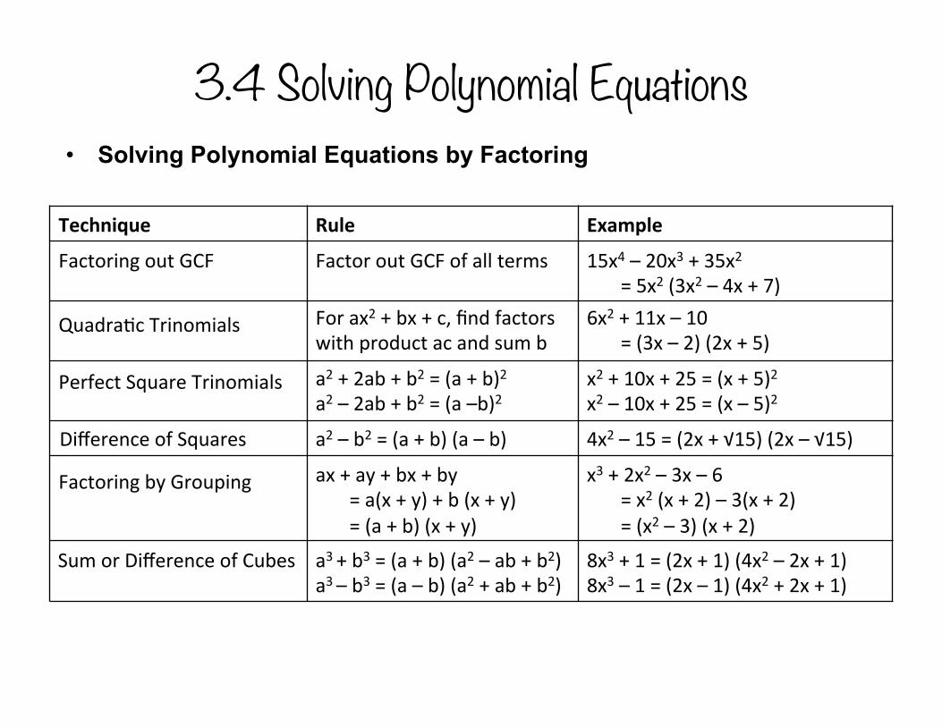
3.4 Solving Polynomial Equations• Solving Polynomial Equations by Factoring
Technique Rule Example
15x4 – 20x3 + 35x2 = 5x2 (3x2 – 4x + 7)
Factor out GCF of all terms Factoring out GCF
Quadra+c Trinomials
Perfect Square Trinomials
Difference of Squares
Factoring by Grouping
Sum or Difference of Cubes
For ax2 + bx + c, find factors with product ac and sum b
6x2 + 11x – 10 = (3x – 2) (2x + 5)
a2 + 2ab + b2 = (a + b)2 a2 – 2ab + b2 = (a –b)2
x2 + 10x + 25 = (x + 5)2 x2 – 10x + 25 = (x – 5)2
a2 – b2 = (a + b) (a – b) 4x2 – 15 = (2x + √15) (2x – √15)
ax + ay + bx + by = a(x + y) + b (x + y) = (a + b) (x + y)
x3 + 2x2 – 3x – 6 = x2 (x + 2) – 3(x + 2) = (x2 – 3) (x + 2)
8x3 + 1 = (2x + 1) (4x2 – 2x + 1) 8x3 – 1 = (2x – 1) (4x2 + 2x + 1)
a3 + b3 = (a + b) (a2 – ab + b2) a3 – b3 = (a – b) (a2 + ab + b2)
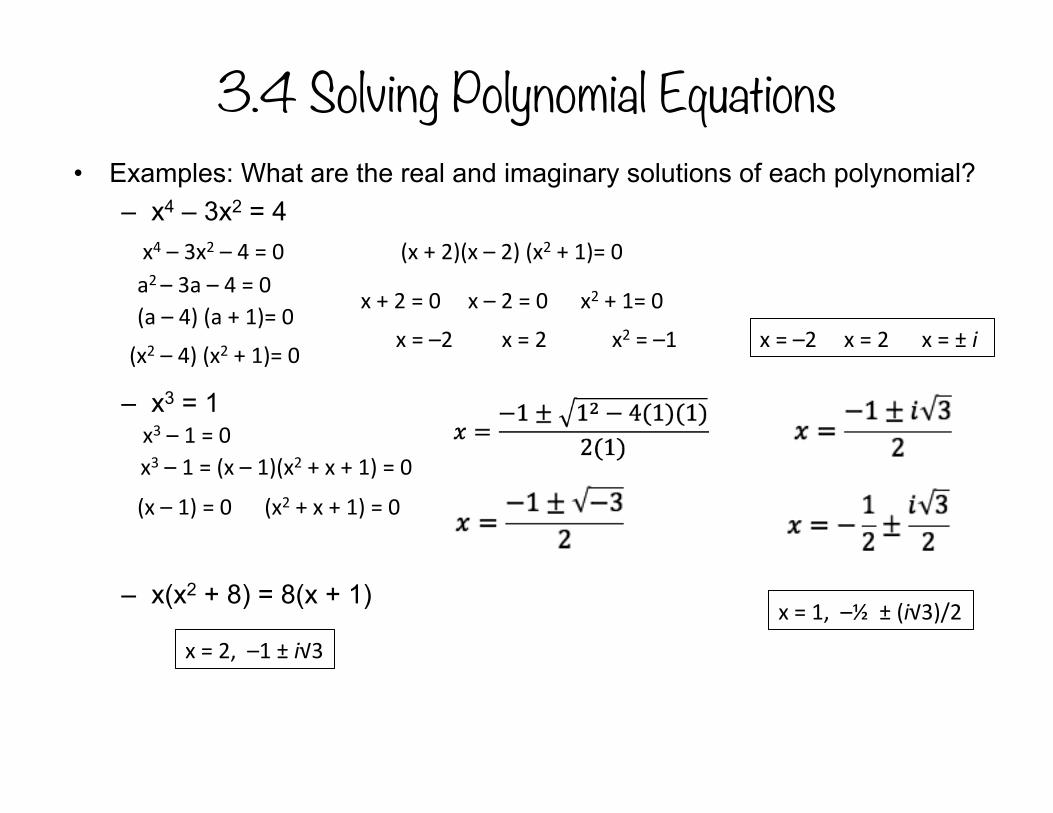
3.4 Solving Polynomial Equations• Examples: What are the real and imaginary solutions of each polynomial?
– x4 – 3x2 = 4
– x3 = 1
– x(x2 + 8) = 8(x + 1)
x4 – 3x2 – 4 = 0 a2 – 3a – 4 = 0 (a – 4) (a + 1)= 0
(x2 – 4) (x2 + 1)= 0
(x + 2)(x – 2) (x2 + 1)= 0
x + 2 = 0 x – 2 = 0 x2 + 1= 0
x = –2 x = 2 x2 = –1 x = –2 x = 2 x = ± i
x = 2, –1 ± i√3
x3 – 1 = 0 x3 – 1 = (x – 1)(x2 + x + 1) = 0
(x – 1) = 0 (x2 + x + 1) = 0
x = 1, –½ ± (i√3)/2
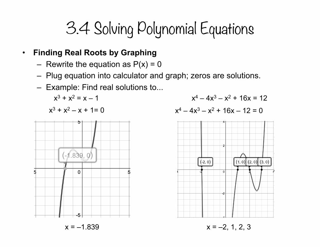
3.4 Solving Polynomial Equations• Finding Real Roots by Graphing
– Rewrite the equation as P(x) = 0 – Plug equation into calculator and graph; zeros are solutions. – Example: Find real solutions to...
x3 + x2 – x + 1= 0
x = –1.839
x3 + x2 = x – 1 x4 – 4x3 – x2 + 16x = 12
x4 – 4x3 – x2 + 16x – 12 = 0
x = –2, 1, 2, 3

3.4 Solving Polynomial Equations• Modeling a Problem Situation
– Close friends Stacy, Una, and Amir were all born on July 4. Stacy is one year younger than Una. Una is two years younger than Amir. On July 4, 2010, the product of their ages was 2300 more than the sum of their ages. How old was each friend on that day?
– What are three consecutive integers whose product is 480 more than their sum?
Let x = Una’s age on July 4, 2010 x – 1 = Stacy’s age x + 2 = Amir’s age
x + (x – 1) + (x + 2) + 2300 = x(x – 1)(x + 2)
3x + 2301 = x(x2 + x – 2)
3x + 2301 = x3 + x2 – 2x
0 = x3 + x2 – 5x – 2301
x = 13
Una was 13, Stacy 12, and Amir 15
7, 8, 9
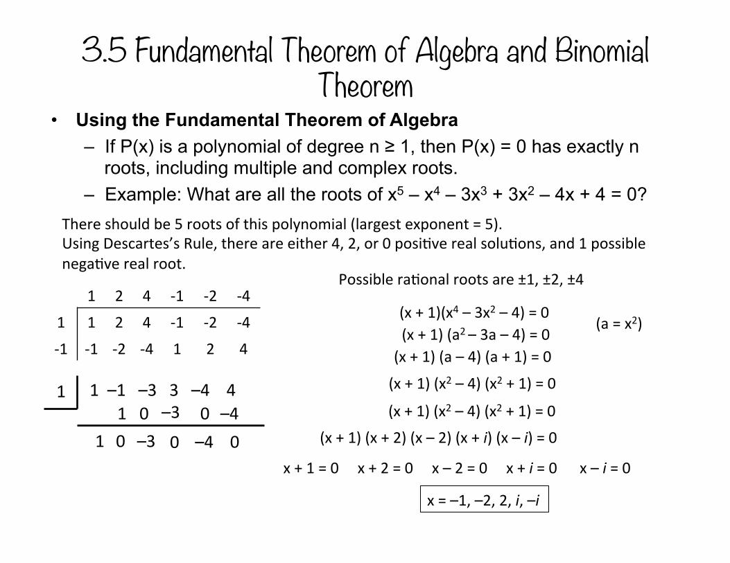
3.5 Fundamental Theorem of Algebra and Binomial Theorem
• Using the Fundamental Theorem of Algebra – If P(x) is a polynomial of degree n ≥ 1, then P(x) = 0 has exactly n
roots, including multiple and complex roots. – Example: What are all the roots of x5 – x4 – 3x3 + 3x2 – 4x + 4 = 0?
There should be 5 roots of this polynomial (largest exponent = 5). Using Descartes’s Rule, there are either 4, 2, or 0 posi+ve real solu+ons, and 1 possible nega+ve real root.
1 2 4 -‐1 -‐2 -‐4
1 1 2 4 -‐1 -‐2 -‐4
-‐1 -‐1 -‐2 -‐4 1 2 4
Possible ra+onal roots are ±1, ±2, ±4
1 1 –1 –3 3 –4 4
11 0
0 –3 0
–3 0 –4
–4 0
(x + 1)(x4 – 3x2 – 4) = 0 (x + 1) (a2 – 3a – 4) = 0 (x + 1) (a – 4) (a + 1) = 0
(x + 1) (x2 – 4) (x2 + 1) = 0
(x + 1) (x2 – 4) (x2 + 1) = 0
(x + 1) (x + 2) (x – 2) (x + i) (x – i) = 0
x + 1 = 0 x + 2 = 0 x – 2 = 0 x + i = 0 x – i = 0
x = –1, –2, 2, i, –i
(a = x2)

3.5 Fundamental Theorem of Algebra and Binomial Theorem
• Finding all the Zeros of a Polynomial Function – You can use the calculator to help you find the real roots – Use these roots and synthetic division to factor down the polynomial – Find the imaginary roots via quadratic formula (or completing the
square) – Example: x4 + x3 – 7x2 – 9x – 18 = f(x)
Real roots are 3 and –3.
3 1 1 –7 –9 –18
13 4
12 5 6
15 18 0
x4 + x3 – 7x2 – 9x – 18 = (x – 3)(x3 + 4x2 + 5x + 6)
–3 1 4 5 6
1–3 1
–3 2
–6
0
= (x – 3)(x + 3)(x2 + x + 2)
The roots are
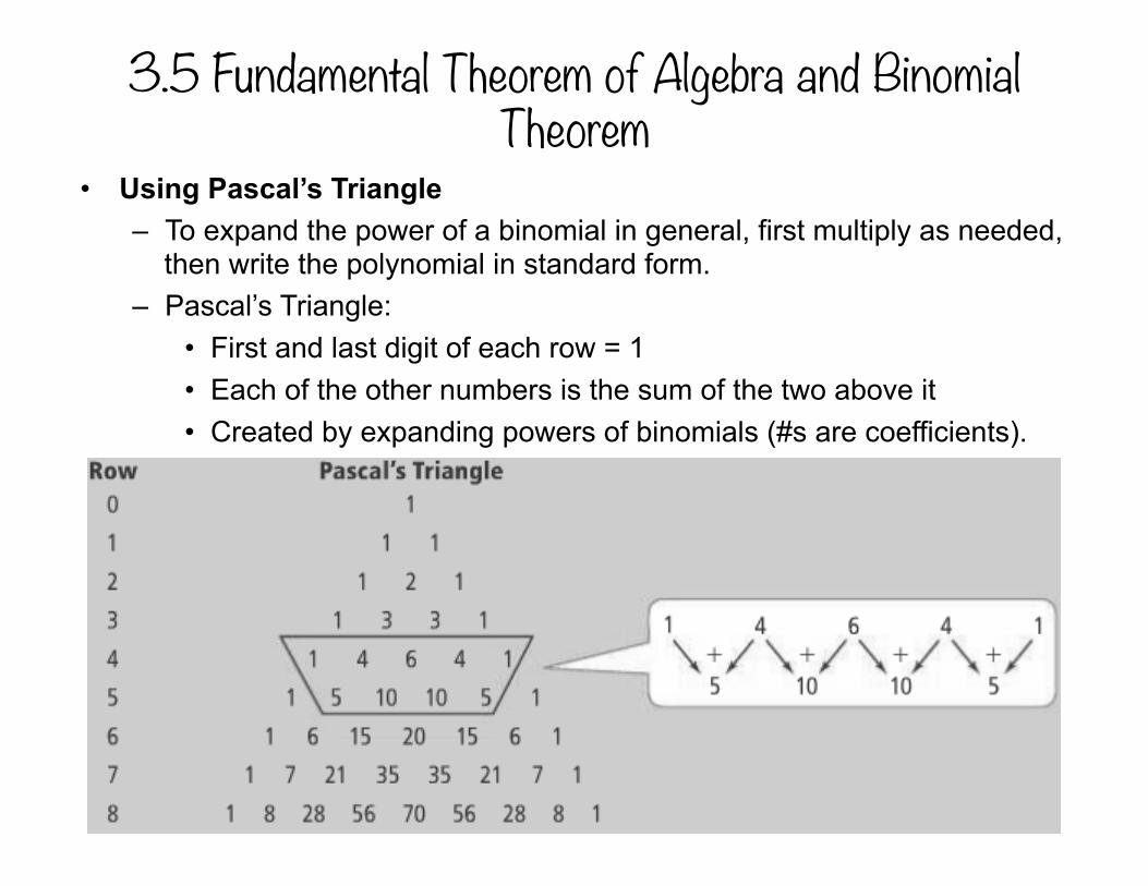
3.5 Fundamental Theorem of Algebra and Binomial Theorem
• Using Pascal’s Triangle – To expand the power of a binomial in general, first multiply as needed,
then write the polynomial in standard form. – Pascal’s Triangle:
• First and last digit of each row = 1 • Each of the other numbers is the sum of the two above it • Created by expanding powers of binomials (#s are coefficients).
3.5 Fundamental Theorem of Algebra and Binomial Theorem
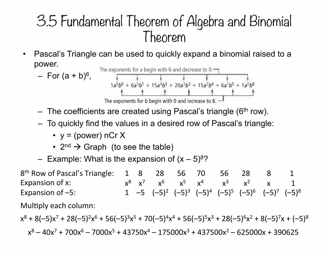
• Pascal’s Triangle can be used to quickly expand a binomial raised to a power. – For (a + b)6,
– The coefficients are created using Pascal’s triangle (6th row). – To quickly find the values in a desired row of Pascal’s triangle:
• y = (power) nCr X • 2nd à Graph (to see the table)
– Example: What is the expansion of (x – 5)8?
1 8 28 56 70 56 28 8 1 8th Row of Pascal’s Triangle: Expansion of x: x8 x7 x6 x5 x4 x3 x2 x 1 Expansion of –5: 1 –5 (–5)2 (–5)3 (–5)4 (–5)5 (–5)6 (–5)7 (–5)8 Mul+ply each column:
x8 – 40x7 + 700x6 – 7000x5 + 43750x4 – 175000x3 + 437500x2 – 625000x + 390625
x8 + 8(–5)x7 + 28(–5)2x6 + 56(–5)3x5 + 70(–5)4x4 + 56(–5)5x3 + 28(–5)6x2 + 8(–5)7x + (–5)8

3.5 Fundamental Theorem of Algebra and Binomial Theorem
• Expanding a Binomial – Binomial Theorem: For every positive integer n,
(a + b)n = P0an + P1an-1b + P2an-2b2 + … + Pn-1abn-1 + Pnbn where P0, P1, ..., Pn are numbers in the nth row of Pascal’s Triangle.
– Example: (x + 2)5
– Example: (3a – 7)3
1 5 10 10 5 1 5th Row of Pascal’s Triangle: Expansion of x: x5 x4 x3 x2 x 1 Expansion of 2: 1 2 22 23 24 25 Mul+ply each column: x5 + 10x4 + 40x3 + 80x2 + 80x + 32
1 3 3 1 3rd Row of Pascal’s Triangle: Expansion of 3a: (3a)3 (3a)2 3a 1 Expansion of (–7): 1 –7 (–7)2 (–7)3 Mul+ply each column: 27a3 – 189a2 + 441a – 343

3.6 Polynomial Models in the Real World and Transforming Polynomial Functions
• Using a Polynomial Function to Model Data
3.6 Polynomial Models in the Real World and Transforming Polynomial Functions
• Modeling Data
3.6 Polynomial Models in the Real World and Transforming Polynomial Functions
• Comparing Models

3.6 Polynomial Models in the Real World and Transforming Polynomial Functions
• Using Interpolation and Extrapolation
3.6 Polynomial Models in the Real World and Transforming Polynomial Functions
• Transforming y = x3.

3.6 Polynomial Models in the Real World and Transforming Polynomial Functions
• Finding Zeros of a Transformed Cubic Function
3.6 Polynomial Models in the Real World and Transforming Polynomial Functions
• Constructing a Quartic Function with Two Real Zeros

3.6 Polynomial Models in the Real World and Transforming Polynomial Functions
• Modeling with a Power Function


