Poles and Zeros First-Order Systems Unit 3: Time Response Part 1: Poles and Zeros and First-Order Systems Engineering 5821: Control Systems I Faculty of Engineering & Applied Science Memorial University of Newfoundland January 28, 2010 ENGI 5821 Unit 3: Time Response
Transcript
Poles and ZerosFirst-Order Systems
Unit 3: Time ResponsePart 1: Poles and Zeros and First-Order Systems
Engineering 5821:Control Systems I
Faculty of Engineering & Applied ScienceMemorial University of Newfoundland
January 28, 2010
ENGI 5821 Unit 3: Time Response
Poles and ZerosFirst-Order Systems
1 Poles and Zeros
1 First-Order Systems
ENGI 5821 Unit 3: Time Response
Poles and ZerosFirst-Order Systems
Poles and Zeros
This unit of the course considers the relationship between asystem’s transfer function and the response of the system in thetime domain.
It corresponds to chapter 4 in the textbook.
The poles and zeros of the input and the transfer function can bequickly inspected to determine the form of the system response.Of course, we can obtain this form from the ILT, but looking atthe poles and zeros allow us to see it more quickly.
ENGI 5821 Unit 3: Time Response
Poles and ZerosFirst-Order Systems
Poles and Zeros
This unit of the course considers the relationship between asystem’s transfer function and the response of the system in thetime domain. It corresponds to chapter 4 in the textbook.
The poles and zeros of the input and the transfer function can bequickly inspected to determine the form of the system response.
Of course, we can obtain this form from the ILT, but looking atthe poles and zeros allow us to see it more quickly.
ENGI 5821 Unit 3: Time Response
Poles and ZerosFirst-Order Systems
Poles and Zeros
This unit of the course considers the relationship between asystem’s transfer function and the response of the system in thetime domain. It corresponds to chapter 4 in the textbook.
The poles and zeros of the input and the transfer function can bequickly inspected to determine the form of the system response.Of course, we can obtain this form from the ILT, but looking atthe poles and zeros allow us to see it more quickly.
ENGI 5821 Unit 3: Time Response
Poles and ZerosFirst-Order Systems
Definitions
The poles of a function are values of s for which the functionbecomes infinite.
e.g. s = −2 is the pole of 1s+2 .
The zeros of a function are values of s for which the functionbecomes zero.
e.g. s = −3 is the zero of s+3s+2 .
Sometimes we also classify as zeros or poles roots of thedenominator (poles) or numerator (zeros) which are common andcan therefore be cancelled. These so-called zeros or poles lack theability to make the function go to zero or infinity, yet aresometimes referred to as zeros or poles nevertheless.
ENGI 5821 Unit 3: Time Response
Poles and ZerosFirst-Order Systems
Definitions
The poles of a function are values of s for which the functionbecomes infinite.
e.g. s = −2 is the pole of 1s+2 .
The zeros of a function are values of s for which the functionbecomes zero.
e.g. s = −3 is the zero of s+3s+2 .
Sometimes we also classify as zeros or poles roots of thedenominator (poles) or numerator (zeros) which are common andcan therefore be cancelled.
These so-called zeros or poles lack theability to make the function go to zero or infinity, yet aresometimes referred to as zeros or poles nevertheless.
ENGI 5821 Unit 3: Time Response
Poles and ZerosFirst-Order Systems
Definitions
The poles of a function are values of s for which the functionbecomes infinite.
e.g. s = −2 is the pole of 1s+2 .
The zeros of a function are values of s for which the functionbecomes zero.
e.g. s = −3 is the zero of s+3s+2 .
Sometimes we also classify as zeros or poles roots of thedenominator (poles) or numerator (zeros) which are common andcan therefore be cancelled. These so-called zeros or poles lack theability to make the function go to zero or infinity, yet aresometimes referred to as zeros or poles nevertheless.
ENGI 5821 Unit 3: Time Response
Poles and ZerosFirst-Order Systems
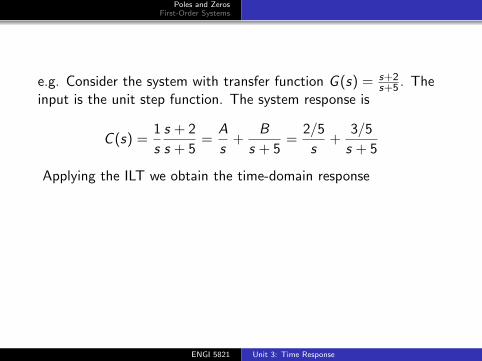
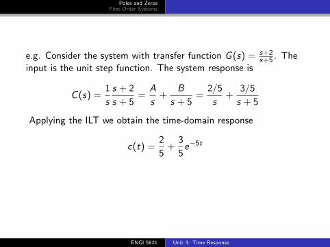
e.g. Consider the system with transfer function G (s) = s+2s+5 .
Theinput is the unit step function. The system response is
C (s) =1
s
s + 2
s + 5=
A
s+
B
s + 5=
2/5
s+
3/5
s + 5
Applying the ILT we obtain the time-domain response
c(t) =2
5+
3
5e−5t
The following figure illustrates the relationship between the systemresponse and the poles and zeros...
ENGI 5821 Unit 3: Time Response
Poles and ZerosFirst-Order Systems
e.g. Consider the system with transfer function G (s) = s+2s+5 . The
input is the unit step function.
The system response is
C (s) =1
s
s + 2
s + 5=
A
s+
B
s + 5=
2/5
s+
3/5
s + 5
Applying the ILT we obtain the time-domain response
c(t) =2
5+
3
5e−5t
The following figure illustrates the relationship between the systemresponse and the poles and zeros...
ENGI 5821 Unit 3: Time Response
Poles and ZerosFirst-Order Systems
e.g. Consider the system with transfer function G (s) = s+2s+5 . The
input is the unit step function. The system response is
C (s) =1
s
s + 2
s + 5
=A
s+
B
s + 5=
2/5
s+
3/5
s + 5
Applying the ILT we obtain the time-domain response
c(t) =2
5+
3
5e−5t
The following figure illustrates the relationship between the systemresponse and the poles and zeros...
ENGI 5821 Unit 3: Time Response
Poles and ZerosFirst-Order Systems
e.g. Consider the system with transfer function G (s) = s+2s+5 . The
input is the unit step function. The system response is
C (s) =1
s
s + 2
s + 5=
A
s+
B
s + 5
=2/5
s+
3/5
s + 5
Applying the ILT we obtain the time-domain response
c(t) =2
5+
3
5e−5t
The following figure illustrates the relationship between the systemresponse and the poles and zeros...
ENGI 5821 Unit 3: Time Response
Poles and ZerosFirst-Order Systems
e.g. Consider the system with transfer function G (s) = s+2s+5 . The
input is the unit step function. The system response is
C (s) =1
s
s + 2
s + 5=
A
s+
B
s + 5=
2/5
s+
3/5
s + 5
Applying the ILT we obtain the time-domain response
c(t) =2
5+
3
5e−5t
The following figure illustrates the relationship between the systemresponse and the poles and zeros...
ENGI 5821 Unit 3: Time Response
Poles and ZerosFirst-Order Systems
e.g. Consider the system with transfer function G (s) = s+2s+5 . The
input is the unit step function. The system response is
C (s) =1
s
s + 2
s + 5=
A
s+
B
s + 5=
2/5
s+
3/5
s + 5
Applying the ILT we obtain the time-domain response
c(t) =2
5+
3
5e−5t
The following figure illustrates the relationship between the systemresponse and the poles and zeros...
ENGI 5821 Unit 3: Time Response
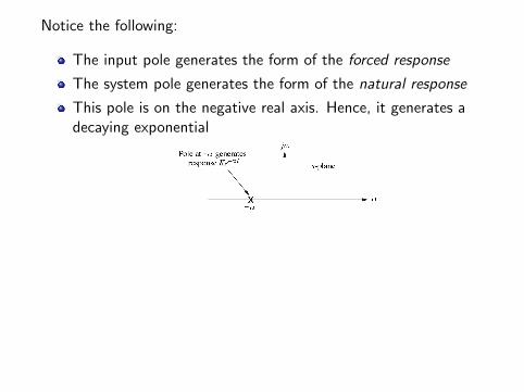
Notice the following:
The input pole generates the form of the forced response
The system pole generates the form of the natural response
This pole is on the negative real axis. Hence, it generates adecaying exponential
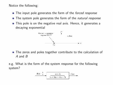
The zeros and poles together contribute to the calculation ofA and B
e.g. What is the form of the system response for the followingsystem?
Notice the following:
The input pole generates the form of the forced response
The system pole generates the form of the natural response
This pole is on the negative real axis. Hence, it generates adecaying exponential
The zeros and poles together contribute to the calculation ofA and B
e.g. What is the form of the system response for the followingsystem?
Poles and ZerosFirst-Order Systems
First-Order Systems
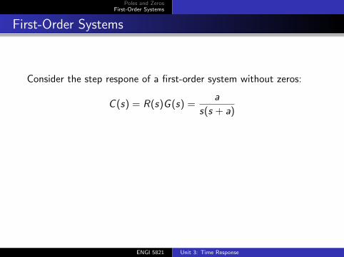
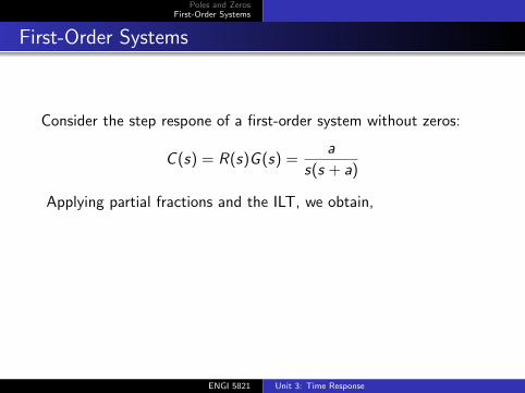
Consider the step respone of a first-order system without zeros:
C (s) = R(s)G (s) =a
s(s + a)
Applying partial fractions and the ILT, we obtain,
c(t) = cf (t) + cn(t) = 1− e−at
The input pole (at s = 0) generates the forced response cf (t) = 1while the system pole yields the natural response cn(t) = −e−at .
ENGI 5821 Unit 3: Time Response
Poles and ZerosFirst-Order Systems
First-Order Systems
Consider the step respone of a first-order system without zeros:
C (s) = R(s)G (s)
=a
s(s + a)
Applying partial fractions and the ILT, we obtain,
c(t) = cf (t) + cn(t) = 1− e−at
The input pole (at s = 0) generates the forced response cf (t) = 1while the system pole yields the natural response cn(t) = −e−at .
ENGI 5821 Unit 3: Time Response
Poles and ZerosFirst-Order Systems
First-Order Systems
Consider the step respone of a first-order system without zeros:
C (s) = R(s)G (s) =a
s(s + a)
Applying partial fractions and the ILT, we obtain,
c(t) = cf (t) + cn(t) = 1− e−at
The input pole (at s = 0) generates the forced response cf (t) = 1while the system pole yields the natural response cn(t) = −e−at .
ENGI 5821 Unit 3: Time Response
Poles and ZerosFirst-Order Systems
First-Order Systems
Consider the step respone of a first-order system without zeros:
C (s) = R(s)G (s) =a
s(s + a)
Applying partial fractions and the ILT, we obtain,
c(t) = cf (t) + cn(t)
= 1− e−at
The input pole (at s = 0) generates the forced response cf (t) = 1while the system pole yields the natural response cn(t) = −e−at .
ENGI 5821 Unit 3: Time Response
Poles and ZerosFirst-Order Systems
First-Order Systems
Consider the step respone of a first-order system without zeros:
C (s) = R(s)G (s) =a
s(s + a)
Applying partial fractions and the ILT, we obtain,
c(t) = cf (t) + cn(t) = 1− e−at
The input pole (at s = 0) generates the forced response cf (t) = 1while the system pole yields the natural response cn(t) = −e−at .
ENGI 5821 Unit 3: Time Response
Poles and ZerosFirst-Order Systems
First-Order Systems
Consider the step respone of a first-order system without zeros:
C (s) = R(s)G (s) =a
s(s + a)
Applying partial fractions and the ILT, we obtain,
c(t) = cf (t) + cn(t) = 1− e−at
The input pole (at s = 0) generates the forced response cf (t) = 1while the system pole yields the natural response cn(t) = −e−at .
ENGI 5821 Unit 3: Time Response
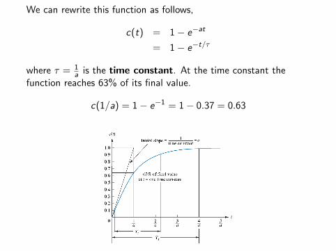
We can rewrite this function as follows,
c(t) = 1− e−at
= 1− e−t/τ
where τ = 1a is the time constant. At the time constant the
function reaches 63% of its final value.
c(1/a) = 1− e−1 = 1− 0.37 = 0.63
We can rewrite this function as follows,
c(t) = 1− e−at
= 1− e−t/τ
where τ = 1a is the time constant. At the time constant the
function reaches 63% of its final value.
c(1/a) = 1− e−1 = 1− 0.37 = 0.63
We can rewrite this function as follows,
c(t) = 1− e−at
= 1− e−t/τ
where τ = 1a is the time constant. At the time constant the
function reaches 63% of its final value.
c(1/a) = 1− e−1 = 1− 0.37 = 0.63
We can rewrite this function as follows,
c(t) = 1− e−at
= 1− e−t/τ
where τ = 1a is the time constant.
At the time constant thefunction reaches 63% of its final value.
c(1/a) = 1− e−1 = 1− 0.37 = 0.63
We can rewrite this function as follows,
c(t) = 1− e−at
= 1− e−t/τ
where τ = 1a is the time constant. At the time constant the
function reaches 63% of its final value.
c(1/a) = 1− e−1 = 1− 0.37 = 0.63
We can rewrite this function as follows,
c(t) = 1− e−at
= 1− e−t/τ
where τ = 1a is the time constant. At the time constant the
function reaches 63% of its final value.
c(1/a) = 1− e−1
= 1− 0.37 = 0.63
We can rewrite this function as follows,
c(t) = 1− e−at
= 1− e−t/τ
where τ = 1a is the time constant. At the time constant the
function reaches 63% of its final value.
c(1/a) = 1− e−1 = 1− 0.37
= 0.63
We can rewrite this function as follows,
c(t) = 1− e−at
= 1− e−t/τ
where τ = 1a is the time constant. At the time constant the
function reaches 63% of its final value.
c(1/a) = 1− e−1 = 1− 0.37 = 0.63
Poles and ZerosFirst-Order Systems
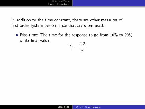
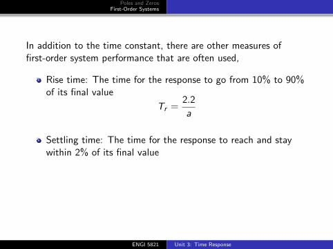
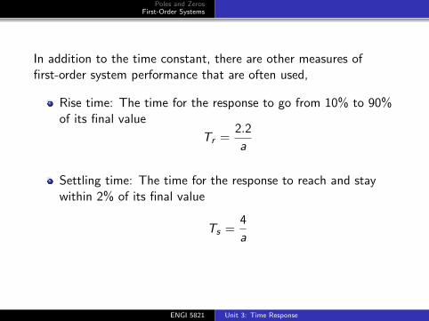
In addition to the time constant, there are other measures offirst-order system performance that are often used,
Rise time: The time for the response to go from 10% to 90%of its final value
Tr =2.2
a
Settling time: The time for the response to reach and staywithin 2% of its final value
Ts =4
a
ENGI 5821 Unit 3: Time Response
Poles and ZerosFirst-Order Systems
In addition to the time constant, there are other measures offirst-order system performance that are often used,
Rise time: The time for the response to go from 10% to 90%of its final value
Tr =2.2
a
Settling time: The time for the response to reach and staywithin 2% of its final value
Ts =4
a
ENGI 5821 Unit 3: Time Response
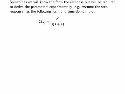
Sometimes we will know the form the response but will be requiredto derive the parameters experimentally.
e.g. Assume the stepresponse has the following form and time-domain plot:
C (s) =K
s(s + a)=
K
a
a
s(s + a)
Determine a and K .
The asymptote yields an estimate of K/a ≈ 0.72. 63% of this is0.45 which is reached around t = 0.15. Hence a = 1/0.15 = 6.67and K = 4.8.
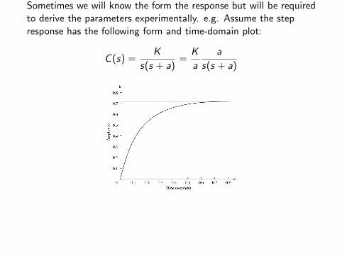
Sometimes we will know the form the response but will be requiredto derive the parameters experimentally. e.g. Assume the stepresponse has the following form and time-domain plot:
C (s) =K
s(s + a)=
K
a
a
s(s + a)
Determine a and K .
The asymptote yields an estimate of K/a ≈ 0.72. 63% of this is0.45 which is reached around t = 0.15. Hence a = 1/0.15 = 6.67and K = 4.8.
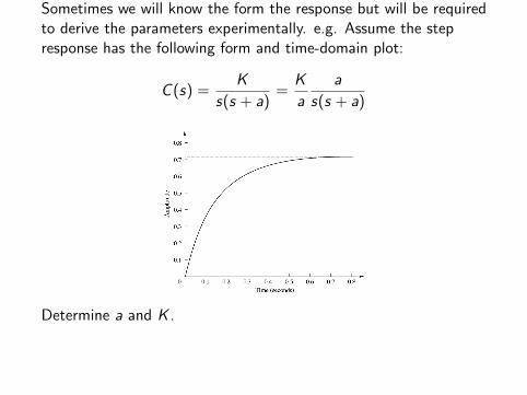
Sometimes we will know the form the response but will be requiredto derive the parameters experimentally. e.g. Assume the stepresponse has the following form and time-domain plot:
C (s) =K
s(s + a)
=K
a
a
s(s + a)
Determine a and K .
The asymptote yields an estimate of K/a ≈ 0.72. 63% of this is0.45 which is reached around t = 0.15. Hence a = 1/0.15 = 6.67and K = 4.8.
Sometimes we will know the form the response but will be requiredto derive the parameters experimentally. e.g. Assume the stepresponse has the following form and time-domain plot:
C (s) =K
s(s + a)=
K
a
a
s(s + a)
Determine a and K .
The asymptote yields an estimate of K/a ≈ 0.72. 63% of this is0.45 which is reached around t = 0.15. Hence a = 1/0.15 = 6.67and K = 4.8.
Sometimes we will know the form the response but will be requiredto derive the parameters experimentally. e.g. Assume the stepresponse has the following form and time-domain plot:
C (s) =K
s(s + a)=
K
a
a
s(s + a)
Determine a and K .
The asymptote yields an estimate of K/a ≈ 0.72.
63% of this is0.45 which is reached around t = 0.15. Hence a = 1/0.15 = 6.67and K = 4.8.
Sometimes we will know the form the response but will be requiredto derive the parameters experimentally. e.g. Assume the stepresponse has the following form and time-domain plot:
C (s) =K
s(s + a)=
K
a
a
s(s + a)
Determine a and K .
The asymptote yields an estimate of K/a ≈ 0.72. 63% of this is0.45 which is reached around t = 0.15.
Hence a = 1/0.15 = 6.67and K = 4.8.
Sometimes we will know the form the response but will be requiredto derive the parameters experimentally. e.g. Assume the stepresponse has the following form and time-domain plot:
C (s) =K
s(s + a)=
K
a
a
s(s + a)
Determine a and K .
The asymptote yields an estimate of K/a ≈ 0.72. 63% of this is0.45 which is reached around t = 0.15. Hence a = 1/0.15 = 6.67and K = 4.8.