Unit 4: Inference for numerical variables Lecture 3: t ...Statistics 104 (Mine C¸etinkaya-Rundel)...

Unit 4: Inference for numerical variablesLecture 3: t-distribution

Statistics 104

Mine Cetinkaya-Rundel

October 22, 2013

Announcements

Project proposal feedback

Cases: units, not valuesData prep:

If categorical, use meaningful level labels that are not justnumbersUse short names for dataset and variable names to streamlineanalysis

Data collection: do not just copy paste from data source, avoidterminology you might not be familiar withType of study:

Avoid generic language in reasoning why the study isobservational/experiment, phrase in context of your data“Variables manipulated?

Statistics 104 (Mine Cetinkaya-Rundel) U4 - L3: t-distribution October 22, 2013 2 / 39

Announcements

Project proposal feedback

Scope of inference: generalizability + causationLarge sample size does not mean generalizability“Population at large”: not informative, define target populationrepresentative sample→ generalizable; random assignment→causal

EDAif using two variables, also include analysis on a single variable(univariate analysis) firstif there are outliers and it makes sense to mention what they are(highest grossing movie, etc.), make sure to mention them in yourdiscussion to provide contextdescribing distributions/comparing groups: also discuss shapeand spread, not just centeravoid repetitive graphs/tabulationssummary([dataset]) is rarely useful

Misccorrelation: association between two numerical variablesdata plural, dataset singular


Small sample inference for the mean

Review: what purpose does a large sample serve?

As long as observations are independent, and the populationdistribution is not extremely skewed, a large sample would ensurethat...

the sampling distribution of the mean is nearly normal

the estimate of the standard error, as s√n, is reliable


Small sample inference for the mean The normality condition

The normality condition

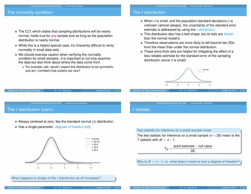
The CLT, which states that sampling distributions will be nearlynormal, holds true for any sample size as long as the populationdistribution is nearly normal.

While this is a helpful special case, it’s inherently difficult to verifynormality in small data sets.We should exercise caution when verifying the normalitycondition for small samples. It is important to not only examinethe data but also think about where the data come from.

For example, ask: would I expect this distribution to be symmetric,and am I confident that outliers are rare?


Small sample inference for the mean Introducing the t distribution

The t distribution

When n is small, and the population standard deviation(σ) isunknown (almost always), the uncertainty of the standard errorestimate is addressed by using the t distribution.This distribution also has a bell shape, but its tails are thickerthan the normal model’s.Therefore observations are more likely to fall beyond two SDsfrom the mean than under the normal distribution.These extra thick tails are helpful for mitigating the effect of aless reliable estimate for the standard error of the samplingdistribution (since n is small)

−4 −2 0 2 4

normalt



The t distribution (cont.)

Always centered at zero, like the standard normal (z) distribution.

Has a single parameter: degrees of freedom (df ).

−2 0 2 4 6

normalt, df=10t, df=5t, df=2t, df=1

What happens to shape of the t distribution as df increases?



t statistic

Test statistic for inference on a small sample mean

The test statistic for inference on a small sample (n < 30) mean is theT statistic with df = n − 1.

Tdf =point estimate − null value

SE

Why is df = n−1, i.e. what does it mean to lose a degree of freedom?


Small sample inference for the mean Example: Friday the 13th

Friday the 13th

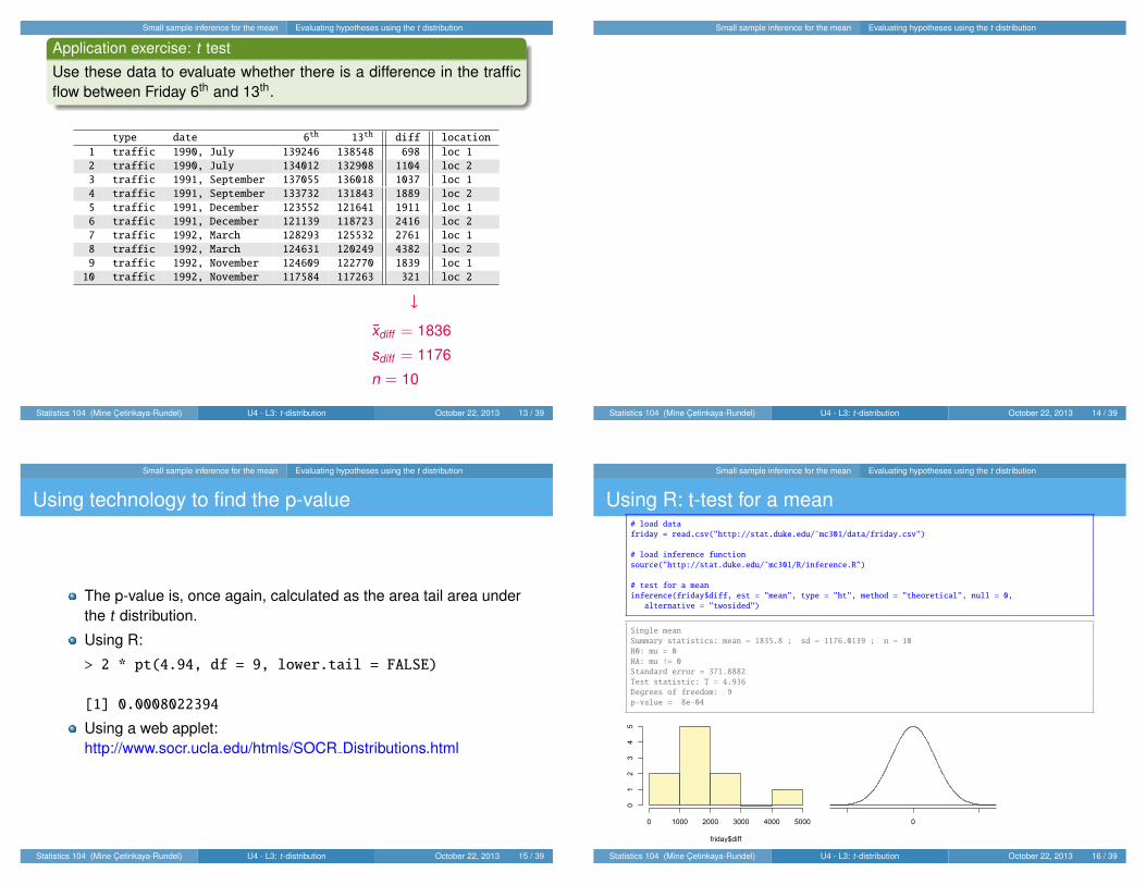
Between 1990 - 1992 researchers in the UK collecteddata on traffic flow, accidents, and hospital admissionson Friday 13th and the previous Friday, Friday 6th.Below is an excerpt from this data set on traffic flow.We can assume that traffic flow on given day atlocations 1 and 2 are independent.

type date 6th 13th diff location

1 traffic 1990, July 139246 138548 698 loc 1

2 traffic 1990, July 134012 132908 1104 loc 2

3 traffic 1991, September 137055 136018 1037 loc 1


5 traffic 1991, December 123552 121641 1911 loc 1


7 traffic 1992, March 128293 125532 2761 loc 1


9 traffic 1992, November 124609 122770 1839 loc 1


Scanlon, T.J., Luben, R.N., Scanlon, F.L., Singleton, N. (1993), “Is Friday the 13th Bad For Your Health?,” BMJ, 307, 1584-1586.



Friday the 13th

We want to investigate if people’s behavior is different on Friday13th compared to Friday 6th.

One approach is to compare the traffic flow on these two days.

H0 : Average traffic flow on Friday 6th and 13th are equal.HA : Average traffic flow on Friday 6th and 13th are different.

Each case in the data set represents traffic flow recorded at the samelocation in the same month of the same year: one count from Friday6th and the other Friday 13th. Are these two counts independent?



Hypotheses

Clicker question

What are the hypotheses for testing for a difference between the aver-age traffic flow between Friday 6th and 13th?

(a) H0 : µ6th = µ13th

HA : µ6th , µ13th

(b) H0 : p6th = p13th

HA : p6th , p13th

(c) H0 : µdiff = 0HA : µdiff , 0

(d) H0 : xdiff = 0HA : xdiff = 0



Conditions

Independence: We are told to assume that cases (rows) areindependent.

Sample size / skew:

The sample distribution does not appear to beextremely skewed, but it’s very difficult to assesswith such a small sample size. We might want tothink about whether we would expect the populationdistribution to be skewed or not – probably not, itshould be equally likely to have days with lower thanaverage traffic and higher than average traffic.

n < 30!

Difference in traffic flow

freq

uenc

y

0 1000 2000 3000 4000 5000

0

1

2

3

4

5

So what do we do when the sample size is small?

We can use simulation, but when working with small sample meanswe can also use the t distribution.


Small sample inference for the mean Evaluating hypotheses using the t distribution

Application exercise: t test

Use these data to evaluate whether there is a difference in the trafficflow between Friday 6th and 13th.

type date 6th 13th diff location

1 traffic 1990, July 139246 138548 698 loc 1

2 traffic 1990, July 134012 132908 1104 loc 2









↓

xdiff = 1836

sdiff = 1176

n = 10





Using technology to find the p-value

The p-value is, once again, calculated as the area tail area underthe t distribution.

Using R:

> 2 * pt(4.94, df = 9, lower.tail = FALSE)

[1] 0.0008022394

Using a web applet:http://www.socr.ucla.edu/htmls/SOCR Distributions.html



Using R: t-test for a mean# load data

friday = read.csv("http://stat.duke.edu/˜mc301/data/friday.csv")

# load inference function

source("http://stat.duke.edu/˜mc301/R/inference.R")

# test for a mean

inference(friday$diff, est = "mean", type = "ht", method = "theoretical", null = 0,

alternative = "twosided")

Single mean

Summary statistics: mean = 1835.8 ; sd = 1176.0139 ; n = 10

H0: mu = 0

HA: mu != 0

Standard error = 371.8882

Test statistic: T = 4.936

Degrees of freedom: 9

p-value = 8e-04

friday$diff

0 1000 2000 3000 4000 5000

01

23

45

0


http://www.socr.ucla.edu/htmls/SOCR_Distributions.html

Small sample inference for the mean Constructing confidence intervals using the t distribution

What is the difference?

We concluded that there is a difference in the traffic flow betweenFriday 6th and 13th.

But it would be more interesting to find out what exactly thisdifference is.

We can use a confidence interval to estimate this difference.



Confidence interval for a small sample mean

Confidence intervals are always of the form

point estimate ±ME

ME is always calculated as the product of a critical value and SE.

Since small sample means follow a t distribution (and not a zdistribution), the critical value is a t? (as opposed to a z?).

point estimate ± t? × SE



Finding the critical t (t?)

0 t* = ?

df = 9

95% n = 10, df = 10 − 1 = 9, t? is atthe intersection of row df = 9 andtwo tail probability 0.05.

one tail 0.100 0.050 0.025 0.010 0.005two tails 0.200 0.100 0.050 0.020 0.010

df 6 1.44 1.94 2.45 3.14 3.717 1.41 1.89 2.36 3.00 3.508 1.40 1.86 2.31 2.90 3.369 1.38 1.83 2.26 2.82 3.25

10 1.37 1.81 2.23 2.76 3.17



Constructing a CI for a small sample mean

Clicker question

Which of the following is the correct calculation of a 95% confidenceinterval for the difference between the traffic flow between Friday 6th

and 13th?

xdiff = 1836 sdiff = 1176 n = 10 SE = 372

(a) 1836 ± 1.96 × 372

(b) 1836 ± 2.26 × 372

(c) 1836 ± −2.26 × 372

(d) 1836 ± 2.26 × 1176



Interpreting the CI

Clicker question

Which of the following is the best interpretation for the confidence in-terval we just calculated?

µdiff :6th−13th = (995, 2677)

We are 95% confident that ...

(a) the difference between the average number of cars on the roadon Friday 6th and 13th is between 995 and 2,677.

(b) on Friday 6th there are 995 to 2,677 fewer cars on the road thanon the Friday 13th, on average.

(c) on Friday 6th there are 995 fewer to 2,677 more cars on the roadthan on the Friday 13th, on average.

(d) on Friday 13th there are 995 to 2,677 fewer cars on the road thanon the Friday 6th, on average.


Small sample inference for the mean Synthesis

Synthesis

Does the conclusion from the hypothesis test agree with the findingsof the confidence interval?

Do the findings of the study suggest that people believe Friday 13th isa day of bad luck?


Small sample inference for the mean Synthesis

Recap: Inference using a small sample mean

If n < 30, and σ is unknown, use the t distribution for inferenceon means.Hypothesis testing:


SE

where df = n − 1 and SE = s√n

Confidence interval:

point estimate ± t?df × SE

Note: The example we used was for paired means (difference between dependent

groups). We took the difference between the observations and used only these

differences (one sample) in our analysis, therefore the mechanics are the same as

when we are working with just one sample.Statistics 104 (Mine Cetinkaya-Rundel) U4 - L3: t-distribution October 22, 2013 23 / 39

The t distribution for the difference of two means

Diamonds

Weights of diamonds are measured in carats.1 carat = 100 points, 0.99 carats = 99 points, etc.The difference between the size of a 0.99 carat diamond and a 1carat diamond is undetectable to the naked human eye, but theprice of a 1 carat diamond tends to be much higher than theprice of a 0.99 diamond.We are going to test to see if there is a difference between theaverage prices of 0.99 and 1 carat diamonds.In order to be able to compare equivalent units, we divide theprices of 0.99 carat diamonds by 99 and 1 carat diamonds by100, and compare the average point prices.



Data

carat = 0.99 carat = 1

20

30

40

50

60

70

80

0.99 carat 1 caratpt99 pt100

x 44.50 53.43s 13.32 12.22n 23 30

These data are a random sample from the diamonds data set in ggplot2 R package.



Parameter and point estimate

Parameter of interest: Average difference between the pointprices of all 0.99 carat and 1 carat diamonds.

µpt99 − µpt100

Point estimate: Average difference between the point prices ofsampled 0.99 carat and 1 carat diamonds.

xpt99 − xpt100



Hypotheses

Clicker question

Which of the following is the correct set of hypotheses for testing ifthe average point price of 1 carat diamonds (pt100) is higher than theaverage point price of 0.99 carat diamonds (pt99)?

(a) H0 : µpt99 = µpt100

HA : µpt99 , µpt100

(b) H0 : µpt99 = µpt100

HA : µpt99 > µpt100

(c) H0 : µpt99 = µpt100

HA : µpt99 < µpt100

(d) H0 : xpt99 = xpt100

HA : xpt99 < xpt100



Conditions

Clicker question

Which of the following does not need to be satisfied in order to conductthis hypothesis test using theoretical methods?

(a) Point price of one 0.99 carat diamond in the sample should beindependent of another, and the point price of one 1 carsdiamond should independent of another as well.

(b) Point prices of 0.99 carat and 1 carat diamonds in the sampleshould be independent.

(c) Distributions of point prices of 0.99 and 1 carat diamonds shouldnot be extremely skewed.

(d) Both sample sizes should be at least 30.


The t distribution for the difference of two means Sampling distribution for the difference of two means

Test statistic

Test statistic for inference on the difference of two small sample means

The test statistic for inference on the difference of two small samplemeans (n1 < 30 and/or n2 < 30) mean is the T statistic.


SE

where

SE =

√s2

1

n1+

s22

n2and df = min(n1 − 1, n2 − 1)

Note: The calculation of the df is actually much more complicated. For simplicity we’ll

use the above formula to estimate the true df when conducting the analysis by hand.


The t distribution for the difference of two means Hypothesis testing for the difference of two means

Test statistic (cont.)

Calculate the test statistic.

0.99 carat 1 caratpt99 pt100

x 44.50 53.43s 13.32 12.22n 23 30

T =point estimate − null value

SE

=(44.50 − 53.43) − 0√

13.322

23 + 12.222

30

=−8.933.56

= −2.508



Test statistic (cont.)

Clicker question

Which of the following is the correct df for this hypothesis test?

(a) 22

(b) 23

(c) 30

(d) 29

(e) 52



p-value

Clicker question

Which of the following is the correct p-value for this hypothesis test?

T = −2.508

(a) between 0.005 and 0.01

(b) between 0.01 and 0.025

(c) between 0.02 and 0.05

(d) between 0.01 and 0.02


df 21 1.32 1.72 2.08 2.52 2.8322 1.32 1.72 2.07 2.51 2.8223 1.32 1.71 2.07 2.50 2.8124 1.32 1.71 2.06 2.49 2.8025 1.32 1.71 2.06 2.49 2.79



Synthesis

What is the conclusion of the hypothesis test? How (if at all) would thisconclusion change your behavior if you went diamond shopping?



Diamond prices

http:// rstudio-pubs-static.s3.amazonaws.com/ 2176 75884214fc524dc0bc2a140573da38bb.html



Using R: t-test for a difference of two means# load data

diamond = read.csv("http://stat.duke.edu/˜mc301/data/diamond.csv")

# test for a difference of means

inference(diamond$ptprice, diamond$carat, est = "mean", type = "ht", method = "theoretical",

null = 0, alternative = "less", order = c("pt99", "pt100"))

Response variable: numerical, Explanatory variable: categorical

Difference between two means

Summary statistics:

n_pt99 = 23, mean_pt99 = 44.5061, sd_pt99 = 13.3239

n_pt100 = 30, mean_pt100 = 53.4337, sd_pt100 = 12.2157

Observed difference between means (pt99-pt100) = -8.9276

H0: mu_pt99 - mu_pt100 = 0

HA: mu_pt99 - mu_pt100 < 0

Standard error = 3.563

Test statistic: T = -2.506

Degrees of freedom: 22

p-value = 0.0101

pt99 pt100

2040

6080

diamond$ptprice

-8.93 0


The t distribution for the difference of two means Confidence intervals for the difference of two means

Equivalent confidence level

Clicker question

What is the equivalent confidence level for a one sided hypothesis testat α = 0.05?

(a) 90%

(b) 92.5%

(c) 95%

(d) 97.5%


http://rstudio-pubs-static.s3.amazonaws.com/2176_75884214fc524dc0bc2a140573da38bb.html


Critical value

Clicker question

What is the appropriate t? for a confidence interval for the averagedifference between the point prices of 0.99 and 1 carat diamonds?

(a) 1.32(b) 1.72(c) 2.07(d) 2.82


df 21 1.32 1.72 2.08 2.52 2.8322 1.32 1.72 2.07 2.51 2.8223 1.32 1.71 2.07 2.50 2.8124 1.32 1.71 2.06 2.49 2.8025 1.32 1.71 2.06 2.49 2.79



Application exercise: t interval for comparing means

Calculate a 90% confidence interval for the average difference be-tween the point prices of 0.99 and 1 carat diamonds?, and interpretit in context.


The t distribution for the difference of two means Recap

Recap: Inference for difference of two small samplemeans

If n1 < 30 and/or n2 < 30 use the t distribution for inference ondifference of means.

Hypothesis testing:


SE

where df = min(n1 − 1, n2 − 1) and SE =

√s2

1n1

+s2

2n2

.

Confidence interval:

point estimate ± t?df × SE


Date post:	20-Feb-2020
Category:	Documents
Upload:	others
View:	7 times
Download:	0 times

Unit 4: Inference for numerical variables Lecture 3: t ...Statistics 104 (Mine C¸etinkaya-Rundel)...

Documents