Unit 64: Thermofluids Unit Workbook 4 - WB 4.pdf · o Fixed inlet vanes – adjustable turbine...

Unit Workbook 4 - Level 5 ENG – U64 Thermofluids © 2018 UniCourse Ltd. All Rights Reserved

Page 1 of 26

Pearson BTEC Level _ Higher Nationals in Engineering (RQF)

Unit 64: Thermofluids

Unit Workbook 4 in a series of 4 for this unit

Learning Outcome 4

Fluid Systems

Sample


Page 5 of 26

4.1 Fluid Flow Fluid flow can be broken down into two terms, either laminar or turbulent. Knowing whether a fluid is

laminar or not is very important in figuring out its characteristics.

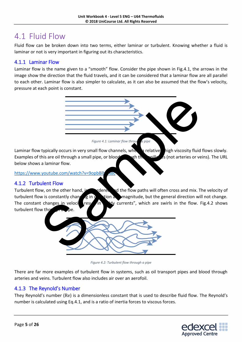
4.1.1 Laminar Flow Laminar flow is the name given to a “smooth” flow. Consider the pipe shown in Fig.4.1, the arrows in the

image show the direction that the fluid travels, and it can be considered that a laminar flow are all parallel

to each other. Laminar flow is also simpler to calculate, as it can also be assumed that the flow’s velocity,

pressure at each point is constant.

Figure 4.1: Laminar flow through a pipe

Laminar flow typically occurs in very small flow channels, where a relatively high viscosity fluid flows slowly.

Examples of this are oil through a small pipe, or blood through the capillaries (not arteries or veins). The URL

below shows a laminar flow.

https://www.youtube.com/watch?v=9opbBlbXN8c

4.1.2 Turbulent Flow Turbulent flow, on the other hand, is disordered and the flow paths will often cross and mix. The velocity of

turbulent flow is constantly changing in direction and magnitude, but the general direction will not change.

The constant changes in velocity result in “eddy currents”, which are swirls in the flow. Fig.4.2 shows

turbulent flow through a pipe.

Figure 4.2: Turbulent flow through a pipe

There are far more examples of turbulent flow in systems, such as oil transport pipes and blood through

arteries and veins. Turbulent flow also includes air over an aerofoil.

4.1.3 The Reynold’s Number They Reynold’s number (Re) is a dimensionless constant that is used to describe fluid flow. The Reynold’s

number is calculated using Eq.4.1, and is a ratio of inertia forces to viscous forces.

Sample

https://www.youtube.com/watch?v=9opbBlbXN8c


Page 7 of 26

4.2 Head Losses in Pipe No system is 100% efficient, and pipework is no exception, frictional losses occur as the surface of the water

and the surface of the pipe make contact with each other.

Head losses in particular describe the loss of pressure in the system, consider the pipework in Fig.4.3 below,

this method is a simple pressure measurement without the use of electronics. The head losses refer to the

height lost at each gauge, the further along the pipe, the more frictional losses occur, this loss in pressure

means that the height that the water reaches in the gauge lowers, and as such h1 > h2 > h3 in Fig.4.3.

Figure 4.3: Head losses in pipes

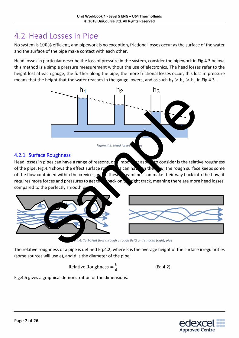
4.2.1 Surface Roughness Head losses in pipes can have a range of reasons, one important aspect to consider is the relative roughness

of the pipe. Fig.4.4 shows the effect surface roughness can have on the flow, the rough surface keeps some

of the flow contained within the crevices, while these streamlines can make their way back into the flow, it

requires more forces and pressures to get them back on the right track, meaning there are more head losses,

compared to the perfectly smooth pipe.

Figure 4.4: Turbulent flow through a rough (left) and smooth (right) pipe

The relative roughness of a pipe is defined Eq.4.2, where k is the average height of the surface irregularities

(some sources will use ϵ), and d is the diameter of the pipe.

Relative Roughness =k

d (Eq.4.2)

Fig.4.5 gives a graphical demonstration of the dimensions.

Sample


Page 8 of 26

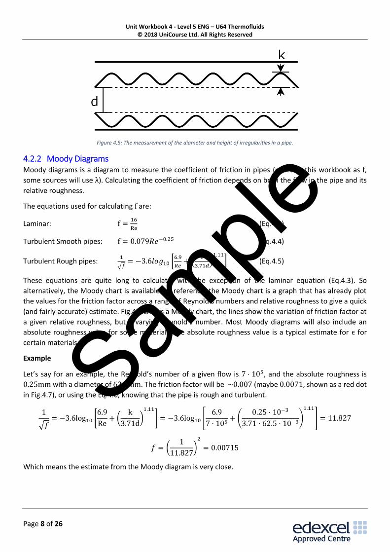
Figure 4.5: The measurement of the diameter and height of irregularities in a pipe.

4.2.2 Moody Diagrams Moody diagrams is a diagram to measure the coefficient of friction in pipes (noted in this workbook as f,

some sources will use λ). Calculating the coefficient of friction depends on both the flow in the pipe and its

relative roughness.

The equations used for calculating f are:

Laminar: f =16

Re (Eq.4.3)

Turbulent Smooth pipes: f = 0.079𝑅𝑒−0.25 (Eq.4.4)

Turbulent Rough pipes: 1

√𝑓= −3.6𝑙𝑜𝑔10 [

6.9

𝑅𝑒+ (

𝜖

3.71𝑑)

1.11

] (Eq.4.5)

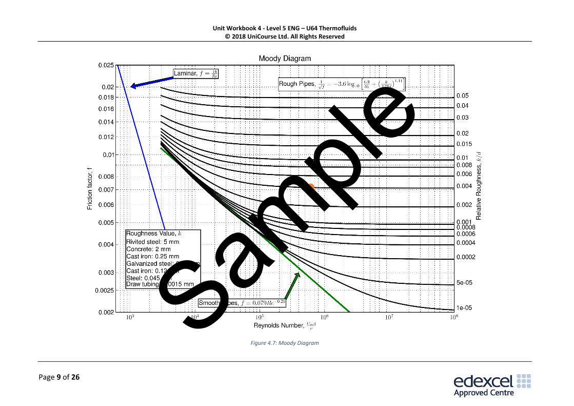
These equations are quite long to calculate, with the exception of the laminar equation (Eq.4.3). So

alternatively, the Moody chart is available for reference, the Moody chart is a graph that has already plot

the values for the friction factor across a range of Reynold’s numbers and relative roughness to give a quick

(and fairly accurate) estimate. Fig.4.6 shows a Moody chart, the lines show the variation of friction factor at

a given relative roughness, but a varying Reynold’s number. Most Moody diagrams will also include an

absolute roughness value for some materials, the absolute roughness value is a typical estimate for ϵ for

certain materials.

Example

Let’s say for an example, the Reynold’s number of a given flow is 7 ⋅ 105, and the absolute roughness is

0.25mm with a diameter of 62.5mm. The friction factor will be ~0.007 (maybe 0.0071, shown as a red dot

in Fig.4.7), or using the Eq.4.6, knowing that the pipe is rough and turbulent.

1

√𝑓= −3.6log10 [

6.9

Re+ (

k

3.71d)

1.11

] = −3.6log10 [6.9

7 ⋅ 105+ (

0.25 ⋅ 10−3

3.71 ⋅ 62.5 ⋅ 10−3)

1.11

] = 11.827

𝑓 = (1

11.827)

2

= 0.00715

Which means the estimate from the Moody diagram is very close.

Sample


Page 9 of 26

Figure 4.7: Moody DiagramSam

ple


Page 10 of 26

4.2.4 The Darcy-Weisbach Equation The Darcy-Weisbach equation is used to calculate the head losses in a system. The head loss of a system is

measured in the height change in metres, and is a valid measurement of pressure drop. The Darcy-Weisbach

equation is defined by Eq.4.6:

ℎ𝑓 =𝑓𝑙𝑢2

2𝑔𝑑 (Eq.4.6)

Where:

• ℎ𝑓 is the head loss (𝑚)

• 𝑓 is the friction factor

• 𝑙 is the length of the pipe (𝑚)

• 𝑢 is the velocity of the fluid (𝑚/𝑠)

• 𝑔 is acceleration due to gravity (𝑚/𝑠2)

• 𝑑 is the diameter of the pipe (𝑚)

Example

An oil Pipeline is transporting Arabian Light oil at 20∘C (v = 10.7mm2/s, ρ = 854kg/m3) over 500m at

1m/s. Calculate the head loss in the pipe if the pipe’s diameter is 20cm with a relative roughness of 0.008.

Answer

Re =𝑢𝐿

𝑣=

1 ⋅ 500

10.7 ⋅ 10−6= 4.67 ⋅ 107

Flow is turbulent, and from the Moody diagram, the friction factor f can be estimated as 0.0089, meaning

that hf can be calculated as:

ℎ𝑓 =𝑓𝑙𝑢2

2𝑔𝑑=

(0.0089)(500)(1)2

2(9.81)(0.2)= 1.13m

By using the equation to find f, we will also need to find the absolute roughness of the system (k), which is:

0.008 ⋅ 0.2 = 0.0016

1

√𝑓= −3.6log10 [

6.9

Re+ (

k

3.71d)

1.11

] = −3.6log10 [6.9

4.67 ⋅ 107+ (

0.0016

3.71 ⋅ 0.2)

1.11

] = 10.6542

𝑓 =1

10.65422= 0.00881

Meaning head loss is:

hf =flu2

2gd=

0.0088(500)(1)2

2(9.81)(0.2)= 1.12m

Again, an almost miniscule difference over 500m of pipe.

Sample


Page 13 of 26

4.3 Turbines Hydraulic Machines are systems that will use the force of water to do work (or vice versa). The earliest

examples of this are the traditional water wheels which date back to roughly 4000 B.C, which were used for

crop irrigation, water transport and grinding grain. As technology advanced, water wheels were used to

power sawmills, bellows and textile mills, before being replaced with fuel powered engines in a lot of

applications.

Turbines use the movement of fluid to generate work, while pumps do work to move fluid. Turbines can be

classed as either an impulse turbine, or a reaction turbine. Reaction turbines move as a result of a reaction

force with the fluid acting on it, while impulse turbines are pushed using an impulse (the rate of change of

momentum) from the fluid.

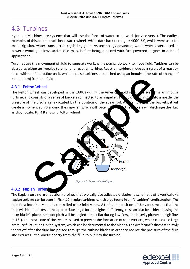
4.3.1 Pelton Wheel The Pelton wheel was developed in the 1800s during the American gold rush. This system is an impulse

turbine, and consists of a series of buckets connected to an impeller. The fluid is fed into a into a nozzle, the

pressure of the discharge is dictated by the position of the spear rod. As the fluid hits the buckets, it will

create a moment acting around the impeller, which will force it to rotate, the buckets will discharge the fluid

as they rotate. Fig.4.9 shows a Pelton wheel.

Figure 4.9: Pelton wheel diagram

4.3.2 Kaplan Turbine The Kaplan turbine are reaction turbines that typically use adjustable blades; a schematic of a vertical-axis

Kaplan turbine can be seen in Fig.4.10, Kaplan turbines can also be found in an “s-turbine” configuration. The

fluid flow into the system is controlled using inlet vanes. Altering the position of the vanes means that the

fluid will hit the rotors at the appropriate angle for the highest efficiency, this can also be achieved using the

rotor blade’s pitch; the rotor pitch will be angled almost flat during low flow, and heavily pitched at high flow

(~45∘). The nose cone of the system is used to prevent the formation of rope vortices, which can cause large

pressure fluctuations in the system, which can be detrimental to the blades. The draft tube’s diameter slowly

tapers off after the fluid has passed through the turbine blades in order to reduce the pressure of the fluid

and extract all the kinetic energy from the fluid to put into the turbine.

Sample


Page 14 of 26

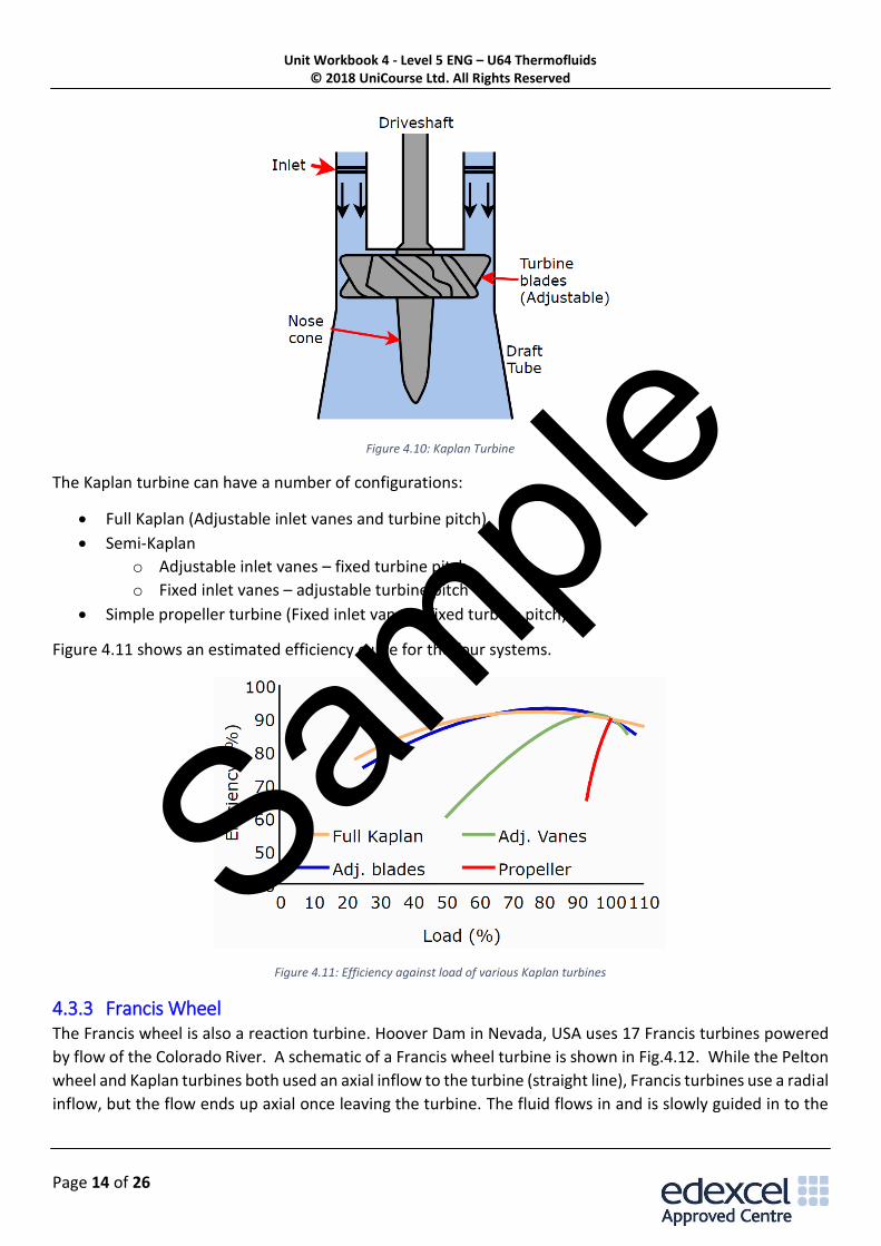
Figure 4.10: Kaplan Turbine

The Kaplan turbine can have a number of configurations:

• Full Kaplan (Adjustable inlet vanes and turbine pitch)

• Semi-Kaplan

o Adjustable inlet vanes – fixed turbine pitch

o Fixed inlet vanes – adjustable turbine pitch

• Simple propeller turbine (Fixed inlet vanes – fixed turbine pitch)

Figure 4.11 shows an estimated efficiency curve for the four systems.

Figure 4.11: Efficiency against load of various Kaplan turbines

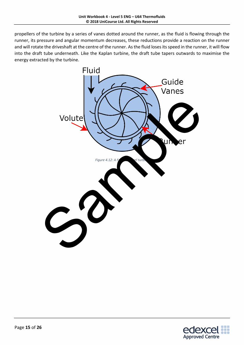
4.3.3 Francis Wheel The Francis wheel is also a reaction turbine. Hoover Dam in Nevada, USA uses 17 Francis turbines powered

by flow of the Colorado River. A schematic of a Francis wheel turbine is shown in Fig.4.12. While the Pelton

wheel and Kaplan turbines both used an axial inflow to the turbine (straight line), Francis turbines use a radial

inflow, but the flow ends up axial once leaving the turbine. The fluid flows in and is slowly guided in to the

Sample


Page 15 of 26

propellers of the turbine by a series of vanes dotted around the runner, as the fluid is flowing through the

runner, its pressure and angular momentum decreases, these reductions provide a reaction on the runner

and will rotate the driveshaft at the centre of the runner. As the fluid loses its speed in the runner, it will flow

into the draft tube underneath. Like the Kaplan turbine, the draft tube tapers outwards to maximise the

energy extracted by the turbine.

Figure 4.12: A Francis wheel turbine

Sample


Page 16 of 26

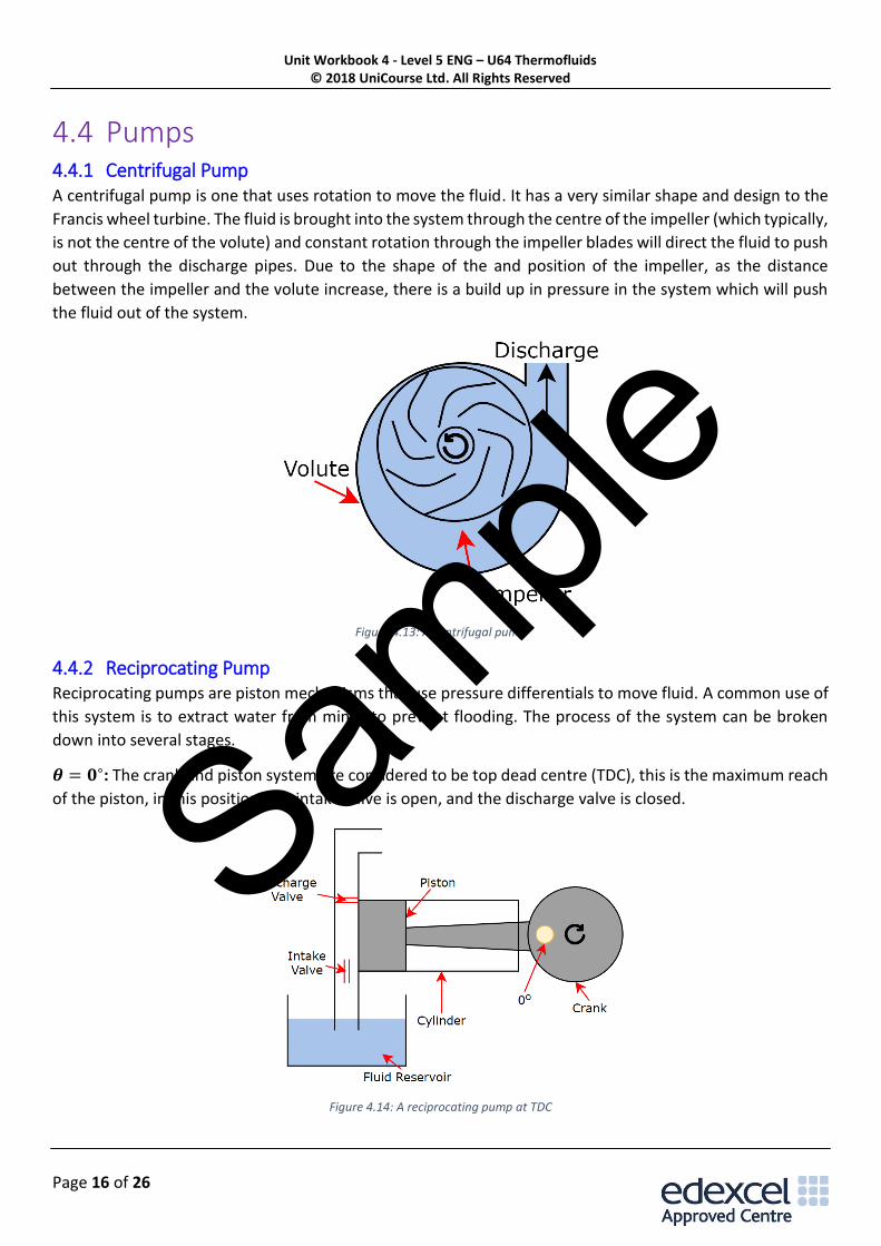
4.4 Pumps 4.4.1 Centrifugal Pump A centrifugal pump is one that uses rotation to move the fluid. It has a very similar shape and design to the

Francis wheel turbine. The fluid is brought into the system through the centre of the impeller (which typically,

is not the centre of the volute) and constant rotation through the impeller blades will direct the fluid to push

out through the discharge pipes. Due to the shape of the and position of the impeller, as the distance

between the impeller and the volute increase, there is a build up in pressure in the system which will push

the fluid out of the system.

Figure 4.13: A centrifugal pump

4.4.2 Reciprocating Pump Reciprocating pumps are piston mechanisms that use pressure differentials to move fluid. A common use of

this system is to extract water from mines to prevent flooding. The process of the system can be broken

down into several stages.

𝜽 = 𝟎∘: The crank and piston system are considered to be top dead centre (TDC), this is the maximum reach

of the piston, in this position, the intake valve is open, and the discharge valve is closed.

Figure 4.14: A reciprocating pump at TDC

Sample


Page 19 of 26

4.5 Dimensional Analysis We can create the equations we use in maths by looking at their dimensions. Which can be broken down

into three distinct dimensions:

• Length [L]

• Mass [M]

• Time [T]

If an equation is dimensionally consistent (RHS=LHS) then the equation maybe accurate (This does not

guarantee it is accurate). Let’s take a look at Newton’s 2nd Law. F = ma, we can break this down into the

three variables and their dimensions.

F = [N] = [M][L][T]−2

m = [M]

a = [𝐿][T]−2

So, when we put this into the equation we get.

[M][L][T]−2 = [M] ⋅ [L][T]−2

Which shows the equation for the Newtons 2nd law as dimensionally consistent.

The same can be said for dimensions, when we calculate Volume, V, we multiply the length, l, by the width,

w, by the depth, d. Shown in the Equation below

V = l ⋅ w ⋅ d

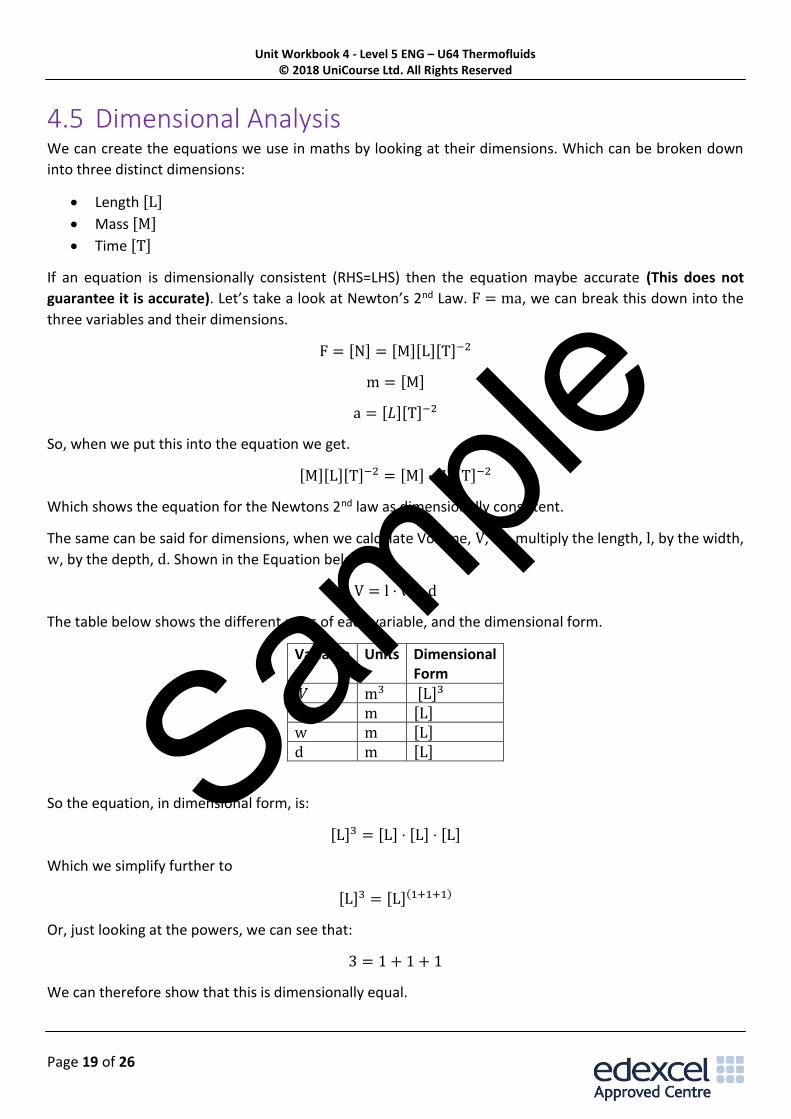
The table below shows the different units of each variable, and the dimensional form.

Variable Units Dimensional Form

𝑉 m3 [L]3 l m [L] w m [L] d m [L]

So the equation, in dimensional form, is:

[L]3 = [L] ⋅ [L] ⋅ [L]

Which we simplify further to

[L]3 = [L](1+1+1)

Or, just looking at the powers, we can see that:

3 = 1 + 1 + 1

We can therefore show that this is dimensionally equal.

Sample


Page 21 of 26

From [3]:

𝐀 = 𝟐 [4]

Sub [4] into [1]:

1 = 1.5(2) + B ∴ 𝐁 = −𝟐

Sub [4] into [2]:

1 = 0.5(2) + C ∴ 𝐂 = 𝟎

Almost there. Earlier we had…

𝐹 ∝ 𝑄𝐴𝑟𝐵𝑚𝐶

Since we know that C = 0 then the ‘m’ term disappears (anything to the power zero is 1). We also know values

for A and B…

𝐹 ∝ 𝑄𝐴𝑟𝐵𝑚𝐶

𝐹 ∝ 𝑄𝐴𝑟𝐵𝑚0

𝐹 ∝ 𝑄𝐴𝑟𝐵

𝐹 ∝ 𝑄2𝑟−2

∴ 𝐹 ∝𝑄2

𝑟2

An important thing to note here; we suspected that the mass of the particles may have had an influence on

the force between them. Our dimensional analysis determined that this was not the case – the mass was

irrelevant. Also, the top of our solution contains a charge squared term, and we know that we had two

charges, Q1 and Q2, so we can confidently write:

𝐹 ∝𝑄1𝑄2

𝑟2

This result looks remarkably like Coulomb’s Law.

However, lets look at a more complicated example.

It is believed that pressure drop ΔP in a pipe is related to the diameter of the pipe d, the length of the pipe

L, the density of the fluid ρ, the dynamic viscosity μ, and the velocity u. Using Rayleigh’s method, determine

the relationship between the variables.

ΔP = daLbρcμdue

Which in dimensional form can be expressed as:

[MLT−2] = [L]a[L]b[ML−3]c[ML−1T−1]d[LT−1]e

Sample


Page 24 of 26

The function can then be written as below, where k and c will be determined by experimentation

ΔP

ρu2= k (

L

d,

μ

ρdu)

c

As all the π groups are dimensionless. It could be a case that the π groups given are the inverse. It is

entirely possible to write:

ρu2

ΔP= k ⋅ f (

d

L,ρdu

μ)

c

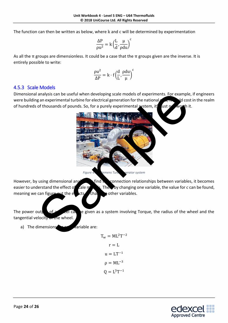
4.5.3 Scale Models Dimensional analysis can be useful when developing scale models of experiments. For example, if engineers

were building an experimental turbine for electrical generation for the national grid, it could cost in the realm

of hundreds of thousands of pounds. So, for a purely experimental system, it’s just not worth it.

Figure 4.19: Siemens Turbogenerator system

However, by using dimensional analysis to find the connection relationships between variables, it becomes

easier to understand the effect of scale models. Then, by changing one variable, the value for c can be found,

meaning we can figure out the effects of changing other variables.

The power output of a wheel can be given as a system involving Torque, the radius of the wheel and the

tangential velocity of the wheel.

a) The dimensions for each variable are:

Tw = ML2T−2

r = L

u = LT−1

ρ = ML−3

Q = L3T−1

Sample


Page 25 of 26

Our recurring set will be:

r = L

u = LT−1

ρ = M𝐿−3

To which the dimensions can be written as:

L = 𝑟

M = ρ𝑟3

T =𝑟

u

So, for Tw:

π1 = Tw × M−1L−2T2

π1 = Tw

1

ρ𝑟3

1

r2

r2

u2

π1 =Tw

ρ𝑟3u2

And for Q:

π2 = Q × L−3𝑇

π2 = Q1

𝑟3

𝑟

𝑢

π2 =Q

r2u

And the π groups are:

Tw

ρ𝑟3u2= k (

Q

r2u)

c

b) If the torque output is proportional to the square of the radius, then we can rearrange to give.

Tw = k (Q

r2u)

c

× ρr3u2

If Tw ∝ r2:

r3 × (1

r2)

c

= r2

Looking at the powers only:

3 − 2c = 2

Sample

Date post:	19-Mar-2020
Category:	Documents
Upload:	others
View:	16 times
Download:	0 times

Unit 64: Thermofluids Unit Workbook 4 - WB 4.pdf · o Fixed inlet vanes – adjustable turbine...

Documents