Unit 8 Chi Square Tests - UMasspeople.umass.edu/~biep540w/pdf/8. chi square tests2010.pdf · We do...

PubHlth 540 – Fall 2010 8. Chi Square Tests Page 1 of 28

Unit 8 Chi Square Tests

“I shall never believe that God plays dice with the world”

- Albert Einstein (1879-1955)

How many patients died? How many travelers on a cruise ship were exposed to contaminated water? How many will vote for Sarah Palin in 2012? And on and on…. So it goes. This unit is about counts. We often have to deal with this kind information. More to the point, this unit is about the analysis of counts relative to some “chance model” expectation. Is the observed count of voters for Sarah Palin in excess of what we might have expected?

Nature Population/ Observation/ Relationships/ Synthesis

Analysis/ Sample Data Modeling


Table of Contents

Topic

1. Unit Roadmap ………………………………………………………..…. 2. Learning Objectives ……………………………………………………… 3. Introduction to Contingency Tables …………………………..………… 4. Introduction to the Contingency Table Hypothesis Test of No Association ……………………………………………..…….…….… 5. The Chi Square Test of No Association in an R x C Table ….……….... 6. (For Epidemiologists) Special Case: More on the 2x2 Table …………. 7. Hypotheses of Independence or No Association …………………..…….

3

4

5

7

13

23

24

Appendix Relationship Between the Normal(0,1) and the Chi Square Distribution .. .

25




1. Unit Roadmap

Nature/

Populations

Sample

Observation/

Data

Relationships

Modeling

Nature Population/ Sample

Observation/ Data

Relationships/ Modeling

Synthesis

Analysis/

Unit 8. Chi Square

Tests

Analysis/ Synthesis

This unit focuses on the analysis of cross-tabulations of counts called contingency tables. Thus, the data are discrete and whole integer. Examples of count data are number of cases of disease, number of cases of exposure, number of events of voter preference, etc The layout of a contingency table is a convenient organization of all the events that could possibly happen. The contingency table then shows the number of times each “contingency” actually occurred in a given sample. Example – Suppose there are 2 “contingencies” for disease (yes or no) and 2 “contingencies” for exposure (yes or no). Between disease and exposure, there are 4 possible combinations or “contingencies”. The analysis of a contingency table requires a model which predicts the expected counts. Lots of models are possible, of course. The simplest model, and the one described in this unit, is the model of independence. The chi square tests described in this unit involve the comparison of observed counts with expected counts, where the expected counts are the predicted counts calculated under the null hypothesis of independence of the “row” and “column” variables.


2. Learning Objectives

When you have finished this unit, you should be able to:

Identify settings where the chi square test is appropriate;

Explain the equivalence of the null hypotheses of “independence”, “no association”, and equality of proportions;

Explain the reasoning that underlies the chi square test of “no association”;

Explain the distinction between “observed” and “expected” counts;

Calculate, by hand, the chi square test of “no association” for a 2x2 table of observed frequencies ;

Outline (and perhaps calculate by hand), the steps in a chi square test of no association for a rxc table of observed frequencies;

Interpret the statistical significance of a chi square test of “no association”.




3. Introduction to Contingency Tables We wish to Explore the Association Between Two Discrete Variables Measuring Counts

• Example - Is smoking associated with low birth weight?

• A common goal of many research studies is investigation of the association of 2 factors, both discrete; eg – smoking (yes/no) and low birth weight (yes/no).

• In Unit 8, our focus is in the setting of two categorical variables, such as smoking and low birth weight, and the use of chi-square tests of association.

Introduction to Contingency Tables

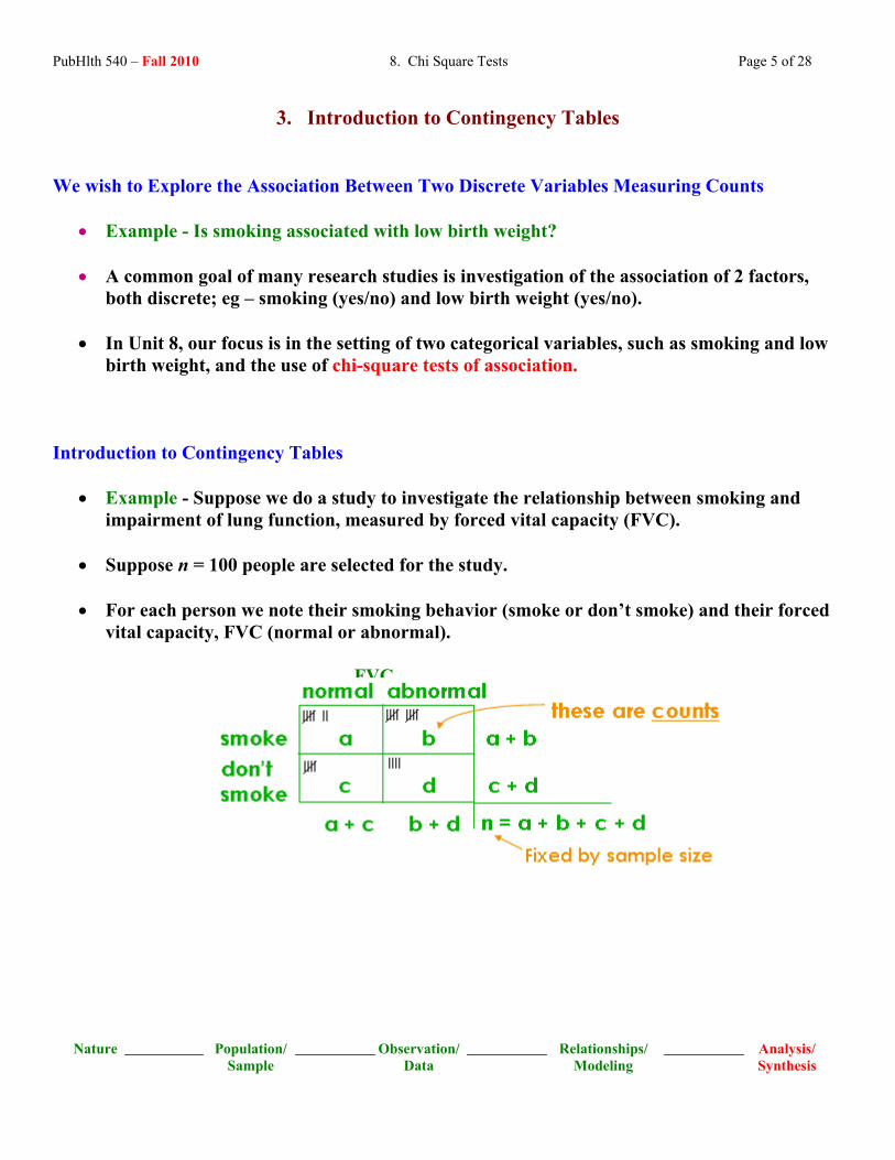
• Example - Suppose we do a study to investigate the relationship between smoking and impairment of lung function, measured by forced vital capacity (FVC).

• Suppose n = 100 people are selected for the study.

• For each person we note their smoking behavior (smoke or don’t smoke) and their forced vital capacity, FVC (normal or abnormal).

FVC




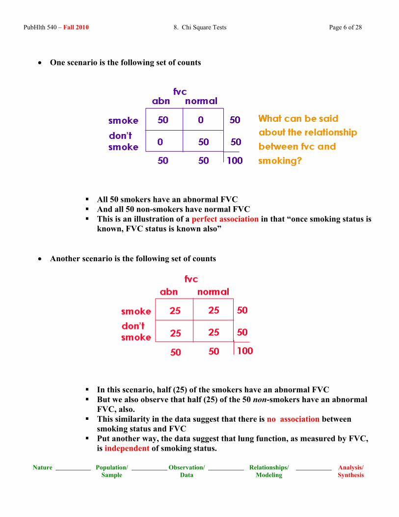
• One scenario is the following set of counts

All 50 smokers have an abnormal FVC And all 50 non-smokers have normal FVC This is an illustration of a perfect association in that “once smoking status is

known, FVC status is known also”

• Another scenario is the following set of counts

In this scenario, half (25) of the smokers have an abnormal FVC But we also observe that half (25) of the 50 non-smokers have an abnormal

FVC, also. This similarity in the data suggest that there is no association between

smoking status and FVC Put another way, the data suggest that lung function, as measured by FVC,

is independent of smoking status.




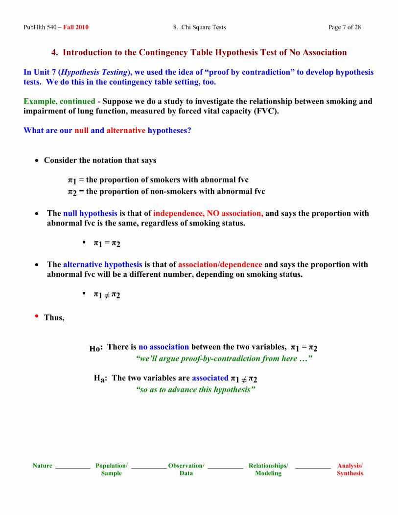
4. Introduction to the Contingency Table Hypothesis Test of No Association In Unit 7 (Hypothesis Testing), we used the idea of “proof by contradiction” to develop hypothesis tests. We do this in the contingency table setting, too. Example, continued - Suppose we do a study to investigate the relationship between smoking and impairment of lung function, measured by forced vital capacity (FVC). What are our null and alternative hypotheses?

• Consider the notation that says π1 = the proportion of smokers with abnormal fvc π2 = the proportion of non-smokers with abnormal fvc

• The null hypothesis is that of independence, NO association, and says the proportion with abnormal fvc is the same, regardless of smoking status.

π1 = π2

• The alternative hypothesis is that of association/dependence and says the proportion with abnormal fvc will be a different number, depending on smoking status.

π1 ≠ π2

• Thus, Ho: There is no association between the two variables, π1 = π2 “we’ll argue proof-by-contradiction from here …”

Ha: The two variables are associated π1 ≠ π2 “so as to advance this hypothesis”




Recall also from Unit 7 that a test statistic (also called pivotal quantity) is a comparison of what the data are to what we expected under the assumption that the null hypothesis is correct – Introduction to observed versus expected counts.

Observed counts are represented using the notation “O” or “n”. Expected counts are represented using the notation “E”

FVC Abnormal Normal

Smoke 11O 12O 1.O

Don’t smoke 21O 22O 2.O

.1O .2O ..O

How to read the subscripts -

o The first subscript tells you the “row” ( e.g. 21O is a cell count in row “2”)

o The second subscript tells you “column” ( e.g. 21O is a cell count in col “1”)

o Thus, 21O is the count for the cell in row “2” and column “1”

o A subscript replaced with a “dot” is tells you what has been totaled over.

Thus, 2.O is the total for row “2” taken over all the columns

Similarly .1O is the total for column “1”, taken over all the rows

And ..O is the grand total taken over all rows and over all columns


Observation/ Data


Synthesis

Analysis/


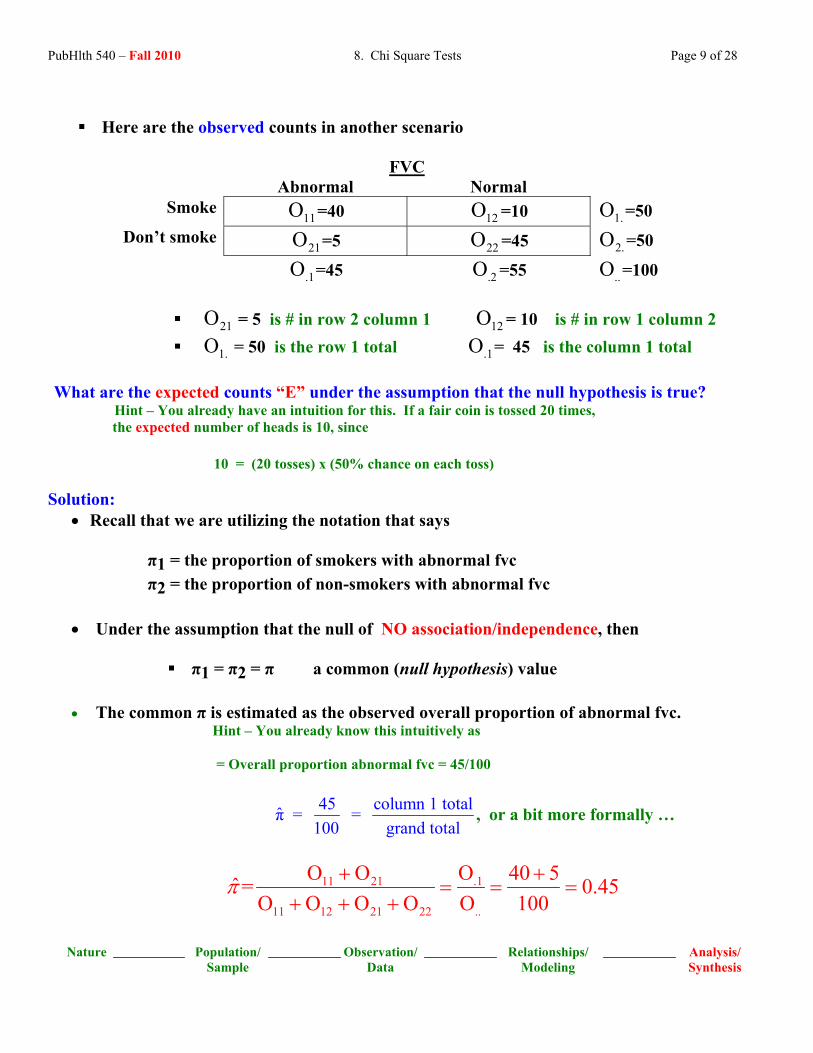
Here are the observed counts in another scenario

FVC Abnormal Normal

Smoke 11O =40 12O =10 1.O =50

Don’t smoke 21O =5 22O =45 2.O =50

.1O =45 .2O =55 ..O =100

21O = 5 is # in row 2 column 1 12O = 10 is # in row 1 column 2 1.O = 50 is the row 1 total .1O = 45 is the column 1 total

What are the expected counts “E” under the assumption that the null hypothesis is true? Hint – You already have an intuition for this. If a fair coin is tossed 20 times, the expected number of heads is 10, since 10 = (20 tosses) x (50% chance on each toss)

Solution: • Recall that we are utilizing the notation that says

π1 = the proportion of smokers with abnormal fvc π2 = the proportion of non-smokers with abnormal fvc

• Under the assumption that the null of NO association/independence, then

π1 = π2 = π a common (null hypothesis) value

• The common π is estimated as the observed overall proportion of abnormal fvc. Hint – You already know this intuitively as

= Overall proportion abnormal fvc = 45/100

45 column 1 totalπ̂ = = 100 grand total

, or a bit more formally …

.111 21

11 12 21 22 ..

OO O 40 5ˆ= 0.45O O O O O 100

π + += = =

+ + +




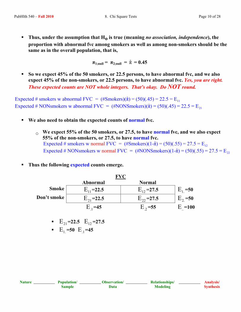
Thus, under the assumption that Ho is true (meaning no association, independence), the

proportion with abnormal fvc among smokers as well as among non-smokers should be the same as in the overall population, that is,

π1;null = π2;null = = 0.45 π̂

So we expect 45% of the 50 smokers, or 22.5 persons, to have abnormal fvc, and we also expect 45% of the non-smokers, or 22.5 persons, to have abnormal fvc. Yes, you are right. These expected counts are NOT whole integers. That’s okay. Do NOT round.

11Êxpected # smokers w abnormal FVC = (#Smokers)(π) = (50)(.45) = 22.5 = E 21Êxpected # NONsmokers w abnormal FVC = (#NONSmokers)(π) = (50)(.45) = 22.5 = E

We also need to obtain the expected counts of normal fvc.

o We expect 55% of the 50 smokers, or 27.5, to have normal fvc, and we also expect

55% of the non-smokers, or 27.5, to have normal fvc. 125 = E

Êxpected # smokers w Frmalno Frmalno

VC = (#Smokers)(1-π) = (50)(.55) = 27.VC = (#NONSmokers)(1-π) = (50)(.55) = 27.5 = E22Êxpected # NONsmokers w

Thus the following expected counts emerge. FVC Abnormal Normal

Smoke 11E =22.5 12E =27.5 1.E =50

Don’t smoke 21E =22.5 22E =27.5 2.E =50

.1E =45 .2E =55 ..E =100

21E =22.5 12E =27.5 1.E =50 .1E =45




• IMPORTANT NOTE about row totals and column totals -

o The expected row totals match the observed row totals.

o The expected column totals match the observed column totals.

o These totals have a special name - “marginals”.

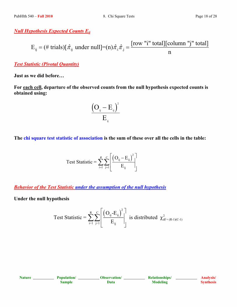
The “marginals” are treated as fixed constants (“givens”). What is the test statistic (pivotal quantity)?

It is a chi square statistic. Examination reveals that it is defined to be a function of the comparisons of observed and expected counts. It can also be appreciated as a kind of “signal-to-noise” construction.

( )2

ij ij2df

all cells "i,j" ij

O EChi Square

Edfχ⎡ ⎤−⎢ ⎥= =⎢ ⎥⎣ ⎦

∑

( )2

ij ij

all cells "i,j" ij

Observed ExpectedExpected

⎡ ⎤−⎢ ⎥=⎢ ⎥⎣ ⎦

∑

• When the null hypothesis of no association is true, the observed and expected counts will be similar, their difference will be close to zero, resulting in a SMALL chi square statistic value.

Example – A null hypothesis says that a coin is “fair”. Since a fair coin tossed 20 times is expected to yield 10 “heads”, the result of 20 tosses is likely to be a number of observed heads that is close to 10.




• When the alternative hypothesis of an association is true the observed counts will be unlike the expected counts, their difference will be non zero and their squared difference will be positive, resulting in a LARGE POSITIVE chi square statistic value. Example – The alternative hypothesis says that a coin is “NOT fair”. An UNfair coin tossed 20 times is expected to yield a different number of heads that is NOT close to the null expectation value of 10.

• Thus, evidence for the rejection of the null hypothesis is reflected in LARGE POSITIVE

values of the chi square statistic.




5. The Chi Square Test of No Association in an R x C Table

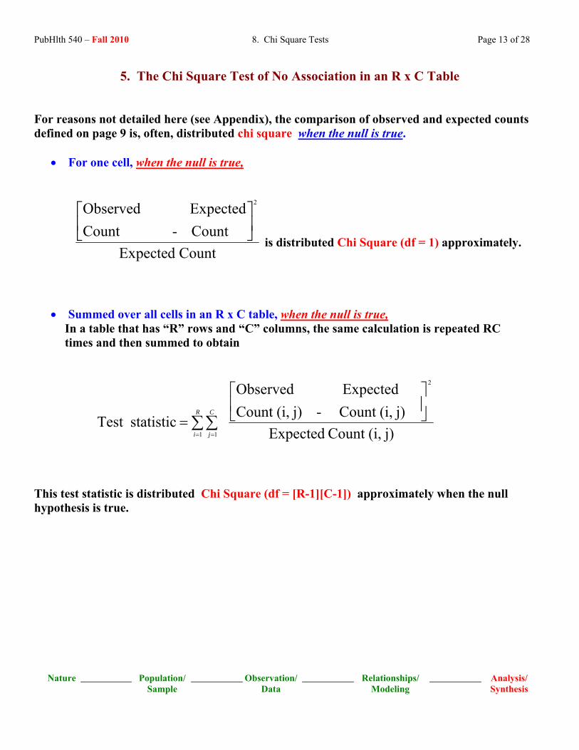
For reasons not detailed here (see Appendix), the comparison of observed and expected counts defined on page 9 is, often, distributed chi square when the null is true.

• For one cell, when the null is true,

Observed ExpectedCount - Count

Expected Count

LNM

OQP

2

is distributed Chi Square (df = 1) approximately.

• Summed over all cells in an R x C table, when the null is true, In a table that has “R” rows and “C” columns, the same calculation is repeated RC times and then summed to obtain

j)(i,Count Expected

j)(i,Count - j)(i,Count Expected Observed

statisticTest

2

1 1

⎥⎦

⎤⎢⎣

⎡

= ∑∑= =

R

i

C

j

This test statistic is distributed Chi Square (df = [R-1][C-1]) approximately when the null hypothesis is true.




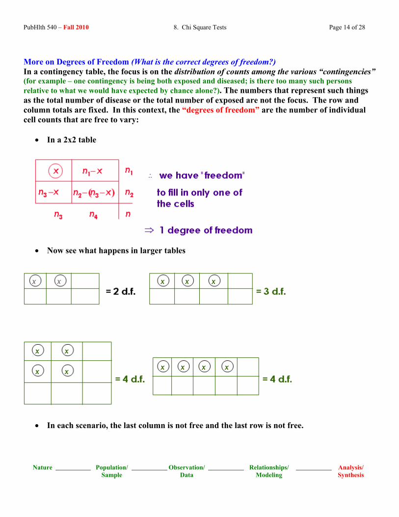
More on Degrees of Freedom (What is the correct degrees of freedom?) In a contingency table, the focus is on the distribution of counts among the various “contingencies” (for example – one contingency is being both exposed and diseased; is there too many such persons relative to what we would have expected by chance alone?). The numbers that represent such things as the total number of disease or the total number of exposed are not the focus. The row and column totals are fixed. In this context, the “degrees of freedom” are the number of individual cell counts that are free to vary:

• In a 2x2 table

• Now see what happens in larger tables

• In each scenario, the last column is not free and the last row is not free.




• More generally,

Degrees of Freedom R x C table = (#rows – 1) x (#columns – 1) = (R – 1)(C – 1)

We have the tools for computing the chi square test of association in a contingency table.

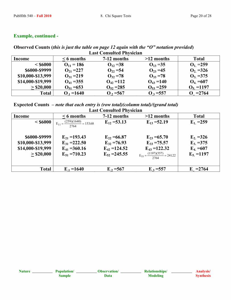
Example Suppose we wish to investigate whether or not there is an association between income level and how regularly a person visits his or her doctor. Consider the following count data.

Last Consulted Physician Income < 6 months 7-12 months >12 months Total

< $6000 186 38 35 259 $6000-$9999 227 54 45 326

$10,000-$13,999 219 78 78 375 $14,000-$19,999 355 112 140 607

> $20,000 653 285 259 1197 Total 1640 567 557 2764

The general layout uses either the “nij” or “Oij” notation to represent the observed counts: Columns, “j” j = 1 … j C= Rows, “I” i = 1 O11=n11 … O1C=n1C N1. = O1. … … i R= OR1=nR1 … ORC=nRC NR. = OR. N.1 = O.1 … N.C = O.C N=O..




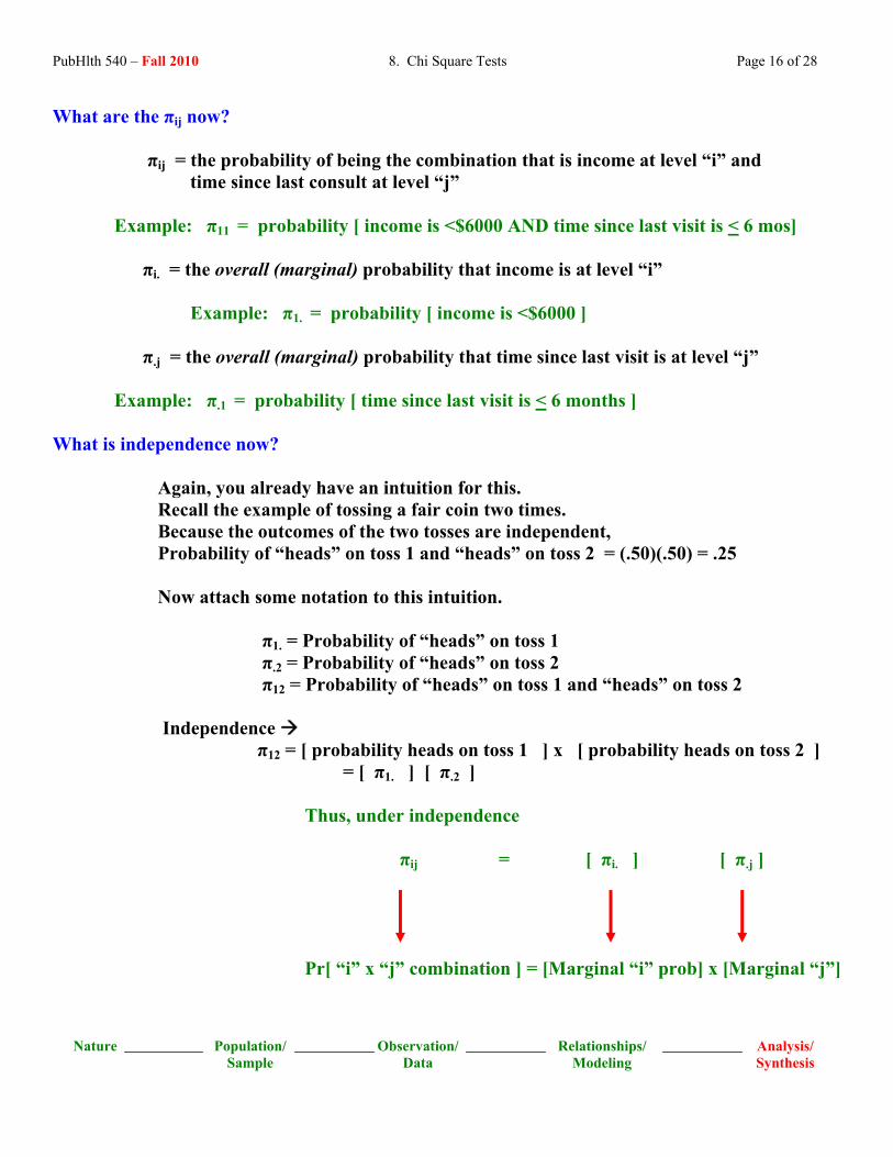
What are the πij now? πij = the probability of being the combination that is income at level “i” and time since last consult at level “j” Example: π11 = probability [ income is <$6000 AND time since last visit is < 6 mos] πi. = the overall (marginal) probability that income is at level “i” Example: π1. = probability [ income is <$6000 ] π.j = the overall (marginal) probability that time since last visit is at level “j” Example: π.1 = probability [ time since last visit is < 6 months ] What is independence now?

Again, you already have an intuition for this. Recall the example of tossing a fair coin two times. Because the outcomes of the two tosses are independent, Probability of “heads” on toss 1 and “heads” on toss 2 = (.50)(.50) = .25 Now attach some notation to this intuition. π1. = Probability of “heads” on toss 1 π.2 = Probability of “heads” on toss 2 π12 = Probability of “heads” on toss 1 and “heads” on toss 2 Independence π12 = [ probability heads on toss 1 ] x [ probability heads on toss 2 ] = [ π1. ] [ π.2 ] Thus, under independence πij = [ πi. ] [ π.j ] Pr[ “i” x “j” combination ] = [Marginal “i” prob] x [Marginal “j”]


Observation/ Data


Synthesis

Analysis/


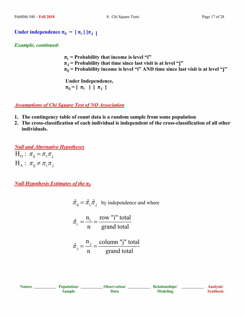
Under independence πij = [ πi. ] [π.j ] Example, continued-

πi. = Probability that income is level “i” π.j = Probability that time since last visit is at level “j” πij = Probability income is level “i” AND time since last visit is at level “j” Under Independence, πij = [ πi. ] [ π.j ]

Assumptions of Chi Square Test of NO Association 1. The contingency table of count data is a random sample from some population 2. The cross-classification of each individual is independent of the cross-classification of all other

individuals. Null and Alternative Hypotheses

O ij i. .jH : π π π=

.j

A ij i.H : π π π≠ Null Hypothesis Estimates of the πij

ij i. .jˆ ˆ ˆπ π π= by independence and where

i.i.

n row "i" totalˆn grand total

π = =

.j.j

n column "j" totalˆn grand total

π = =




Null Hypothesis Expected Counts Eij

ij ij i. .j[row "i" total][column "j" total]ˆ ˆ Ê (# trials)[ under null]=(n)

nπ π π= =

Test Statistic (Pivotal Quantity)

ust as we did before…

or each cell

J F , departure of the observed counts from the null hypothesis expected counts is

obtained using:

O EE

ij ij

ij

−c h2

he chi square test statistic of association is the sum of these over all the cells in the table:

T

( )2

ij ij

1 1 ij

O ETest Statistic =

E

R C

i j= =

⎡ ⎤−⎢ ⎥⎢ ⎥⎣ ⎦

∑∑

ehavior of the Test Statistic under the assumption of the null hypothesis B

Under the null hypothesis

( )2R C

ij ij 2df = (R-1)(C-1)

i=1 j=1 ij

O -ETest Statistic = is distributed χ

E

⎡ ⎤⎢ ⎥⎢ ⎥⎣ ⎦

∑∑




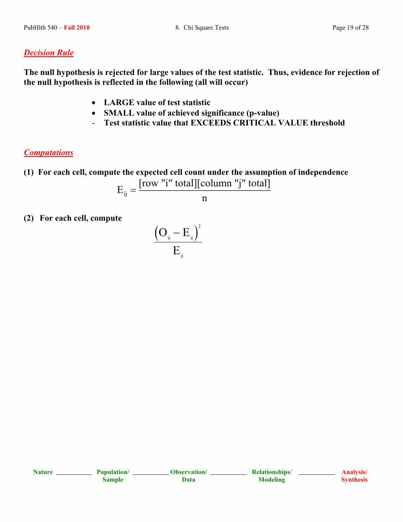
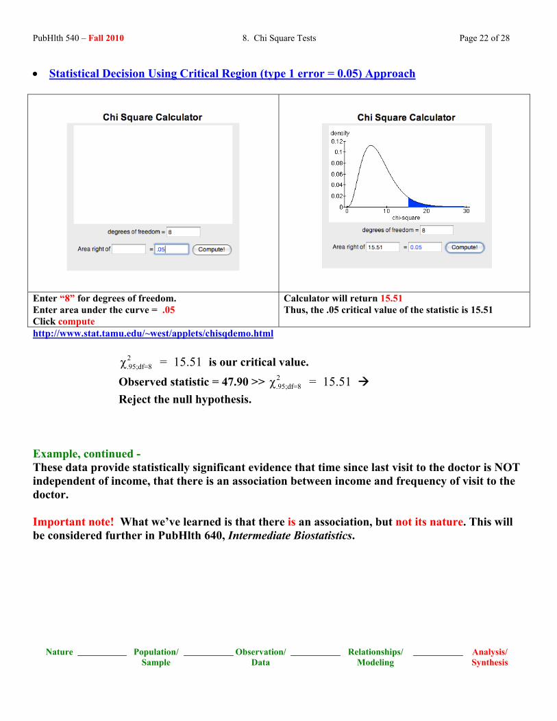
Decision Rule The null hypothesis is rejected for large values of the test statistic. Thus, evidence for rejection of the null hypothesis is reflected in the following (all will occur)

• LARGE value of test statistic • SMALL value of achieved significance (p-value) - Test statistic value that EXCEEDS CRITICAL VALUE threshold

Computations (1) For each cell, compute the expected cell count under the assumption of independence

ij[row "i" total][column "j" total]E

n=

(2) For each cell, compute

O E

Eij ij

ij

−c h2




Example, continued - Observed Counts (this is just the table on page 12 again with the “O” notation provided)


< $6000 O11 = 186 O12 =38 O13 =35 O1. =259 $6000-$9999 O21 =227 O22 =54 O23 =45 O2. =326

$10,000-$13,999 O31 =219 O32 =78 O33 =78 O3. =375 $14,000-$19,999 O41 =355 O42 =112 O43 =140 O4. =607

> $20,000 O51 =653 O52 =285 O53 =259 O5. =1197 Total O.1 =1640 O.2 =567 O.3 =557 O.. =2764

Expected Counts – note that each entry is (row total)(column total)/(grand total)


< $6000 E11 = =( )( ) .259 1640

2764153 68

E12 =53.13 E13 =52.19 E1. =259

$6000-$9999 E21 =193.43 E22 =66.87 E23 =65.70 E2. =326 $10,000-$13,999 E31 =222.50 E32 =76.93 E33 =75.57 E3. =375 $14,000-$19,999 E41 =360.16 E42 =124.52 E43 =122.32 E4. =607

> $20,000 E51 =710.23 E52 =245.55 E53 = =( )( ) .1197 557

276424122

E5. =1197

Total E.1 =1640 E.2 =567 E.3 =557 E.. =2764




( ) ( ) ( )2 2 2

ij ij2( 1)( 1)

all cells ij

O E 186 153.68 259 241.22... 47.90

E 153.68 241.22R Cχ − −

⎡ ⎤− − −⎢ ⎥= = + +⎢ ⎥⎣ ⎦

∑ =

with degrees of freedom = (R-1)(C-1) = (5-1)(3-1) = 8 • Statistical Decision Using Significance Level (p-value) Approach

Enter “8” for degrees of freedom. Calculator will return 0.0000 Enter test statistic value 47.90 Click compute

Thus, p-value < < 0.0001

http://www.stat.tamu.edu/~west/applets/chisqdemo.html

p-value = Probability [ Chi square with df=8 >


Analysis/

47.90 ] < < .0001 Such an extremely small p-value is statistically significant Reject the null hypothesis.

Sample Data Modeling


Statistical Decision Using Critical Region (type 1 error = 0.05) Approach


Analysis/

•

Enter “8” for degrees of freedom. Enter area under the curve = .05

Calculator will return 15.51 Thus, the .05 critical value of the statistic is 15.51

Click compute http://www.stat.tamu.edu/~west/applets/chisqdemo.html

value.

15.51

xample, continued - hese data provide statistically significant evidence that time since last visit to the doctor is NOT

, that there is an association between income and frequency of visit to the

nt note! What we’ve learned is that there is an association, but not its nature. This will e considered further in PubHlth 640, Intermediate Biostatistics.

2

.95;df=8χ = 15.51 is our critical

Observed statistic = 47.90 >> .95;df=8χ =2

Reject the null hypothesis. ETindependent of incomedoctor. Importab

Sample Data Modeling


6. (For Epidemiologists) Special Case: More on the 2x2 Table Many epidemiology texts use a different notation for representing counts in the same chi square test of no association in a 2x2 table. Counts are “a”, “b”, “c”, and “d” as follows. 2nd Classification Variable 1 2 1st Classification 1 a b a + b 2 c d c + d a + c b + d n The calculation for the chi square test that you’ve learned as being given by

( )2

ij ij2

all cells ij

O EE

χ−

= ∑

is the same calculation as the following shortcut formula

( )

( )( )( )( )

22 n ad-bc

a+c b+d c+d a+bχ =

when the notation for the cell entries is the “a”, “b”, “c”, and “d”, above.




7. Hypotheses of Independence or No Association

“Independence”, “No Association”, “Homogeneity of Proportions” are alternative wordings for the same thing. For example,

(1) “Length of time since last visit to physician” is independent of “income” means that income has no bearing on the elapsed time between visits to a physician. The expected elapsed time is the same regardless of income level.

(2) There is no association between coffee consumption and lung cancer means that an individual’s likelihood of lung cancer is not affected by his or her coffee consumption.

(3) The equality of probability of success on treatment (experimental versus standard of care) in a randomized trial of two groups is a test of homogeneity of proportions.

The hypotheses of “independence”, “no association”, “homogeneity of proportions” are equivalent wordings of the same null hypothesis in an analysis of contingency table data.




Appendix Relationship Between the Normal(0,1) and the Chi Square Distributions

For the interested reader ….. This appendix explains how it is reasonable to use a continuous probability model distribution (the chi square) for the analysis of discrete (counts) data, in particular, investigations of association in a contingency table.

• Previously (see Unit 6, Estimation), we obtained a chi square random variable when working with a function of the sample variance S2.

• It is also possible to obtain a chi square random variable as the square of a Normal(0,1) variable. Recall that this is what we have so far …

IF THEN Has a Chi Square Distribution with DF =

Z has a distribution that is Normal (0,1)

Z2

1

X has a distribution that is Normal (μ, σ2), so that

Z - score = X - μσ

{ Z-score }2

1

X1, X2, …, Xn are each distributed Normal (μ, σ2) and are independent, so that X is Normal (μ, σ2/n) and

Z - score = X -nμ

σ

{ Z-score }2

1

X1, X2, …, Xn are each distributed Normal (μ, σ2) and are independent and we calculate

SX - X

2 =−

=∑b g2

1

1i

n

n

(n -1)S2

2σ

(n-1)




Our new formulation of a chi square random variable comes from working with a Bernoulli, the sum of independent Bernoulli random variables, and the central limit theorem. What we get is a great result. The chi square distribution for a continuous random variable can be used as a good model for the analysis of discrete data, namely data in the form of counts.

Z1, Z2, …, Zn are each Bernoulli with probability of event = π. iE[Z ] μ π= =

2iVar[Z ] (1 )σ π π= = −

↓

1. The net number of events is Binomial (N,π) X = Zi

i=1

n

∑ 2. We learned previously that the distribution of the average

of the Zi is well described as Normal(μ, σ2/n).

Apply this notion here: By convention,

Z =Z

nXn

Xi

i 1

n

=∑

= =

↓

3. So perhaps the distribution of the sum is also well described as Normal. At least approximately If X is described well as Normal (μ, σ2/n) Then X = nX is described well as Normal (nμ, nσ2) ↓

Exactly: X is distributed Binomial(n,π) Approximately: X is distributed Normal (nμ, nσ2) Where: =μ π and 2 (1- )σ π π=




Putting it all together … IF

THEN

Comment

X has a distribution that is Binomial (n,π) exactly

X has a distribution that is Normal (nμ, nσ2 ) approximately, where μ = π σ2 = π(1-π) ↓

Z - score = X - E(X)

SD(X)

=X - n

nμσ

X-n

n (1- )π

π π=

is approx. Normal(0,1) ↓

{ Z-score }2 has distribution that is well described as Chi Square with df = 1.

We arrive at a continuous distribution model (chi square)approximation for count data.




Thus, the { Z-score }2 that is distributed approximately Chi Square (df=1) is the (O-E)2/E introduced previously.

• Preliminaries X = “Observed” = O

nπ = "Expected" = E

• As n gets larger and larger nπ(1- ) nπ( 1 ) = "Expected" = Eπ →

• Upon substitution,

{ } ( )2 2 22

2 O-EX-nπ X-nπ O-EZ-Score = = =Enπ(1-π) nπ(1) E

⎧ ⎫ ⎧ ⎫⎪ ⎪ ⎪ ⎪ ⎧ ⎫→⎨ ⎬ ⎨ ⎬ ⎨ ⎬⎩ ⎭⎪ ⎪ ⎪ ⎪⎩ ⎭ ⎩ ⎭

Thus,

• For one cell, when the null hypothesis is true, the central limit theorem gives us


Expected Count

LNM

OQP

2

is Chi Square (df = 1) approximately.

• For RC cells, when the null hypothesis is true, the central limit theorem and the definition

of the chi square distribution give us

2

ij ij

1 1 ij


Expected Count

R C

i J= =

⎡ ⎤⎢ ⎥⎣∑∑ ⎦ is Chi Square [df =(R-1)(C- 1)] approx.



Date post:	04-Sep-2019
Category:	Documents
Upload:	others
View:	5 times
Download:	0 times

Unit 8 Chi Square Tests - UMasspeople.umass.edu/~biep540w/pdf/8. chi square tests2010.pdf · We do...

Documents