69
Monitor Unit Calculations for Photon and Electrons AAPM Spring Meeting March 17, 2013 John P. Gibbons Chief of Clinical Physics
| Date post: | 01-Feb-2018 |
| Category: |
Documents |
| Upload: | truongkhuong |
| View: | 224 times |
| Download: | 1 times |

Monitor Unit Calculations for Photon and Electrons
AAPM Spring MeetingMarch 17, 2013
John P. Gibbons Chief of Clinical Physics
Outline
I. TG71 Formation and ChargeII. Photon CalculationsIII. Electron CalculationsIV. Conclusions
TG‐71Task Group Charge
• Emphasize the importance of a unified methodology
• Recommend of consistent terminology for MU calcs
• Recommend measurement and/or calculation methods
• Recommend QA tests
• Provide example calculations for common clinical setups

TG71 Report Outline1. Introduction2. Nomenclature3. Calculation Formalism
1. MU Equations2. Input Parameters (Depth, Field Size)
4. Measurements5. Interface to TPS6. Quality Assurance7. Examples
Monitor Unit CalculationsOverview
• Accuracy within ±5%• Absolute versus Relative Dosimetry • Consistency with Treatment Plan• QA program
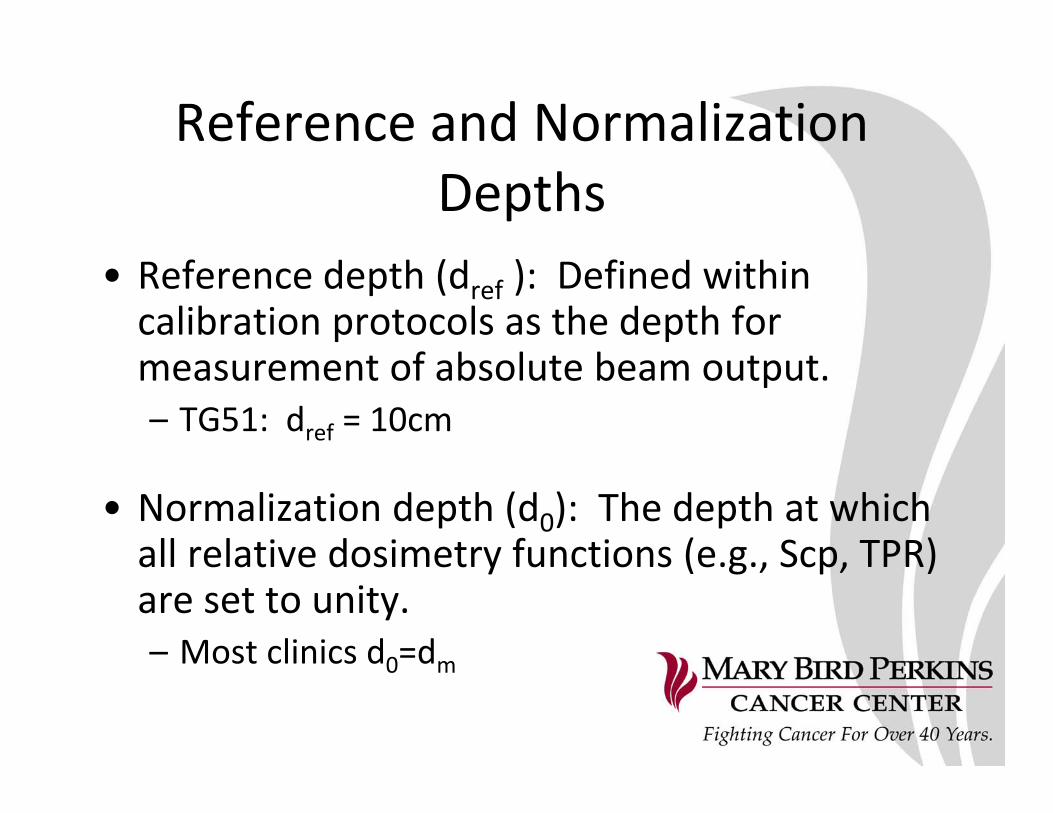
Reference and Normalization Depths
• Reference depth (dref ): Defined within calibration protocols as the depth for measurement of absolute beam output.– TG51: dref = 10cm
• Normalization depth (d0): The depth at which all relative dosimetry functions (e.g., Scp, TPR) are set to unity.– Most clinics d0=dm
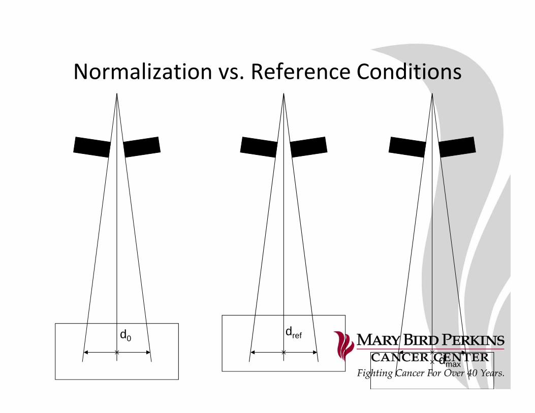
Normalization vs. Reference Conditions
d0dref
dmax
Outline
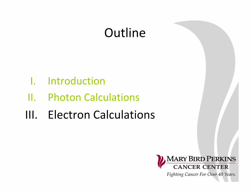
I. Introduction
II. Photon CalculationsIII. Electron Calculations

Nomenclature Principals(3 Laws of Nomenclature)
• Law 1: Use commonly understood symbols• Law 2: Maintain consistency with other TG
reports, unless it conflicts with Law 1• Law 3: Avoid multiple‐letter subscripts
and/or variables, unless it conflicts with Laws 1 or 2
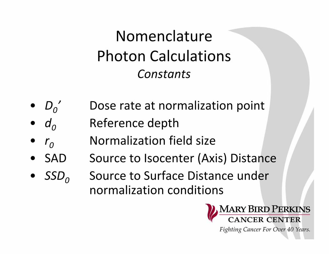
NomenclaturePhoton Calculations
Constants
• D0’ Dose rate at normalization point• d0 Reference depth• r0 Normalization field size• SAD Source to Isocenter (Axis) Distance• SSD0 Source to Surface Distance under
normalization conditions
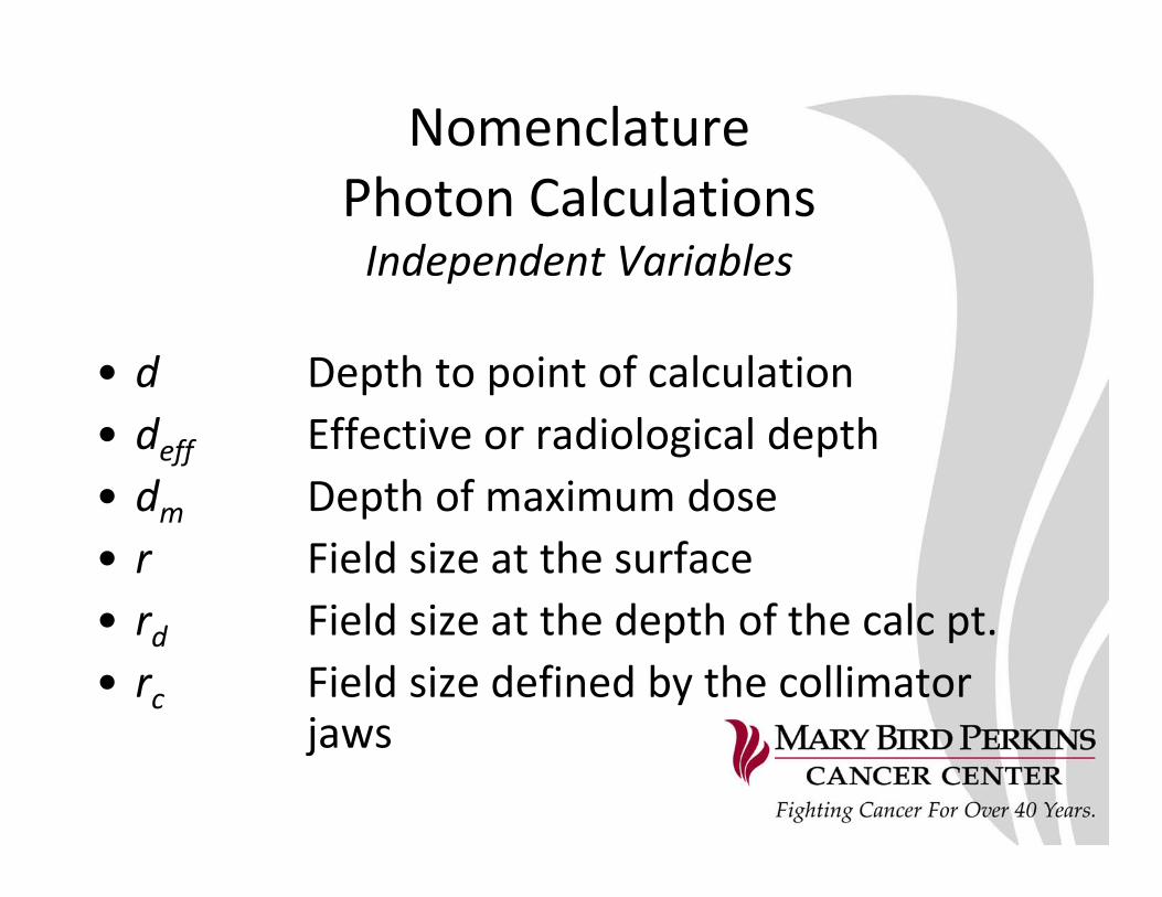
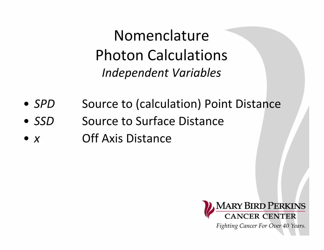
NomenclaturePhoton CalculationsIndependent Variables
• d Depth to point of calculation• deff Effective or radiological depth• dm Depth of maximum dose• r Field size at the surface• rd Field size at the depth of the calc pt.• rc Field size defined by the collimator
jaws
NomenclaturePhoton CalculationsIndependent Variables
• SPD Source to (calculation) Point Distance• SSD Source to Surface Distance• x Off Axis Distance
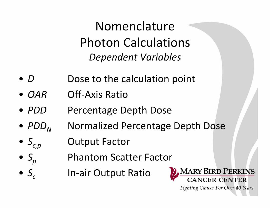
NomenclaturePhoton CalculationsDependent Variables
• D Dose to the calculation point• OAR Off‐Axis Ratio• PDD Percentage Depth Dose• PDDN Normalized Percentage Depth Dose• Sc,p Output Factor• Sp Phantom Scatter Factor• Sc In‐air Output Ratio
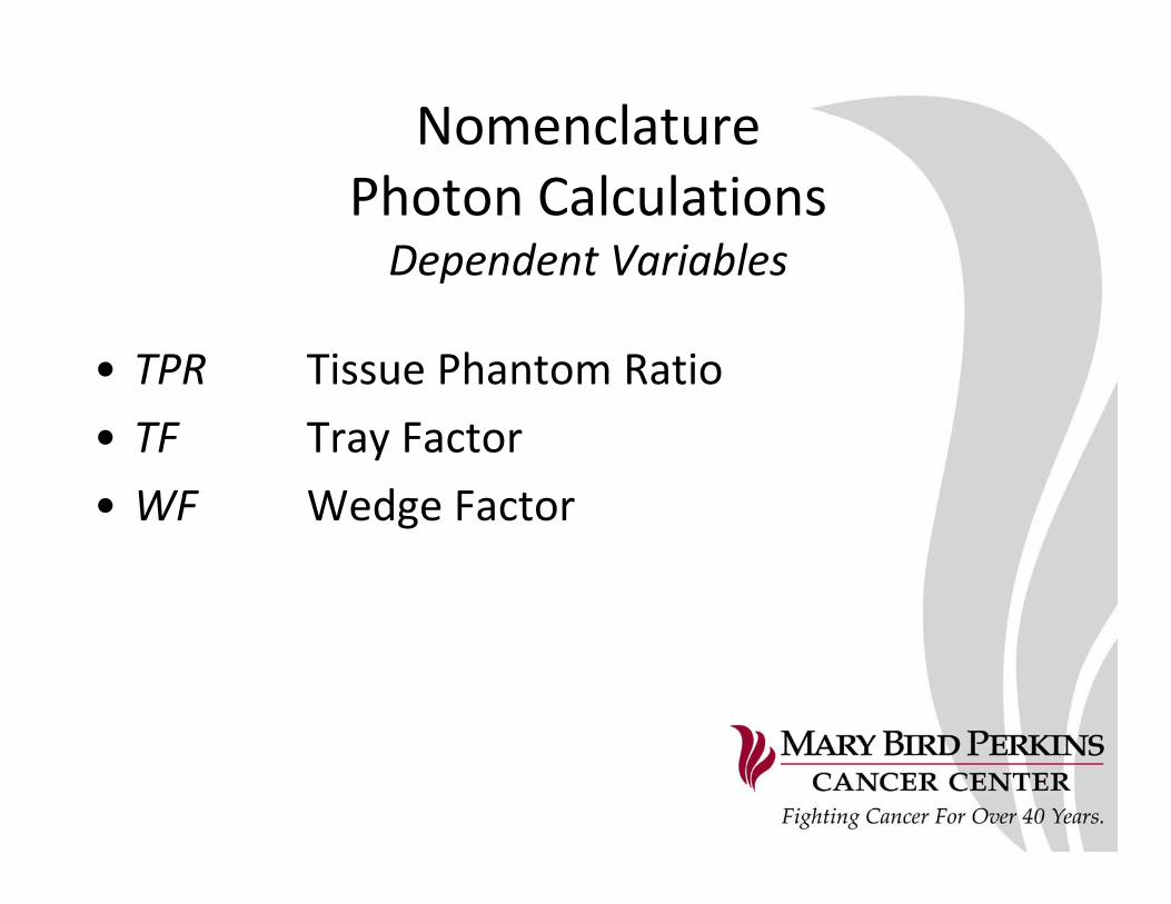
NomenclaturePhoton CalculationsDependent Variables
• TPR Tissue Phantom Ratio• TF Tray Factor• WF Wedge Factor
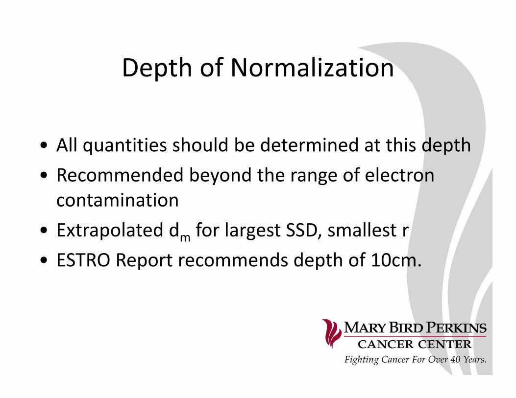
Depth of Normalization
• All quantities should be determined at this depth• Recommended beyond the range of electron contamination
• Extrapolated dm for largest SSD, smallest r• ESTRO Report recommends depth of 10cm.
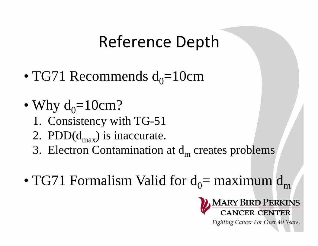
Reference Depth
• TG71 Recommends d0=10cm
• Why d0=10cm?1. Consistency with TG-512. PDD(dmax) is inaccurate.3. Electron Contamination at dm creates problems
• TG71 Formalism Valid for d0= maximum dm

Isocentric CalculationsCalculation to the Isocenter
2
' 0 0
0( ) ( ) ( , ) ( , )
c c p d d d
DMUSSD dD S r S r TPR d r WF d r TF
SAD
=+⎛ ⎞⋅ ⋅ ⋅ ⋅ ⋅ ⋅ ⎜ ⎟
⎝ ⎠

Isocentric CalculationsCalculations to Arbitrary Points
2
' 0 0
0( ) ( ) ( , ) ( , ) ( , )
c c p d d d
DM USSD dD S r S r TPR d r WF d r TF OAR d x
SPD
=+⎛ ⎞⋅ ⋅ ⋅ ⋅ ⋅ ⋅ ⋅ ⎜ ⎟
⎝ ⎠
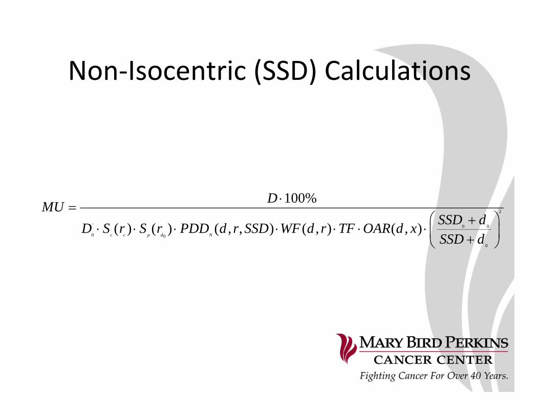
Non‐Isocentric (SSD) Calculations
2
' 0 0
0 0
0
100%
( ) ( ) ( , , ) ( , ) ( , )c c p d N
DMUSSD dD S r S r PDD d r SSD WF d r TF OAR d xSSD d
⋅=
⎛ ⎞+⋅ ⋅ ⋅ ⋅ ⋅ ⋅ ⋅ ⎜ ⎟+⎝ ⎠
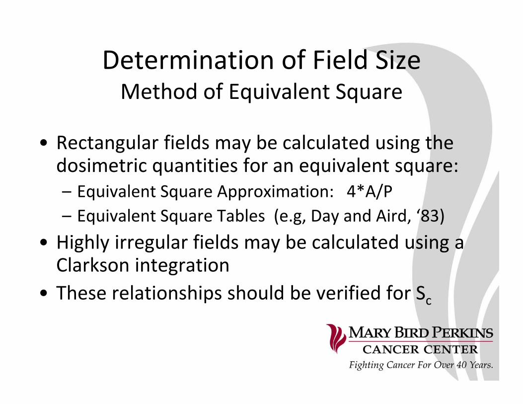
Determination of Field SizeMethod of Equivalent Square
• Rectangular fields may be calculated using the dosimetric quantities for an equivalent square:– Equivalent Square Approximation: 4*A/P– Equivalent Square Tables (e.g, Day and Aird, ‘83)
• Highly irregular fields may be calculated using a Clarkson integration
• These relationships should be verified for Sc
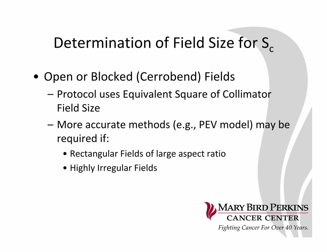
Determination of Field Size for Sc
• Open or Blocked (Cerrobend) Fields– Protocol uses Equivalent Square of Collimator Field Size
– More accurate methods (e.g., PEV model) may be required if:• Rectangular Fields of large aspect ratio• Highly Irregular Fields

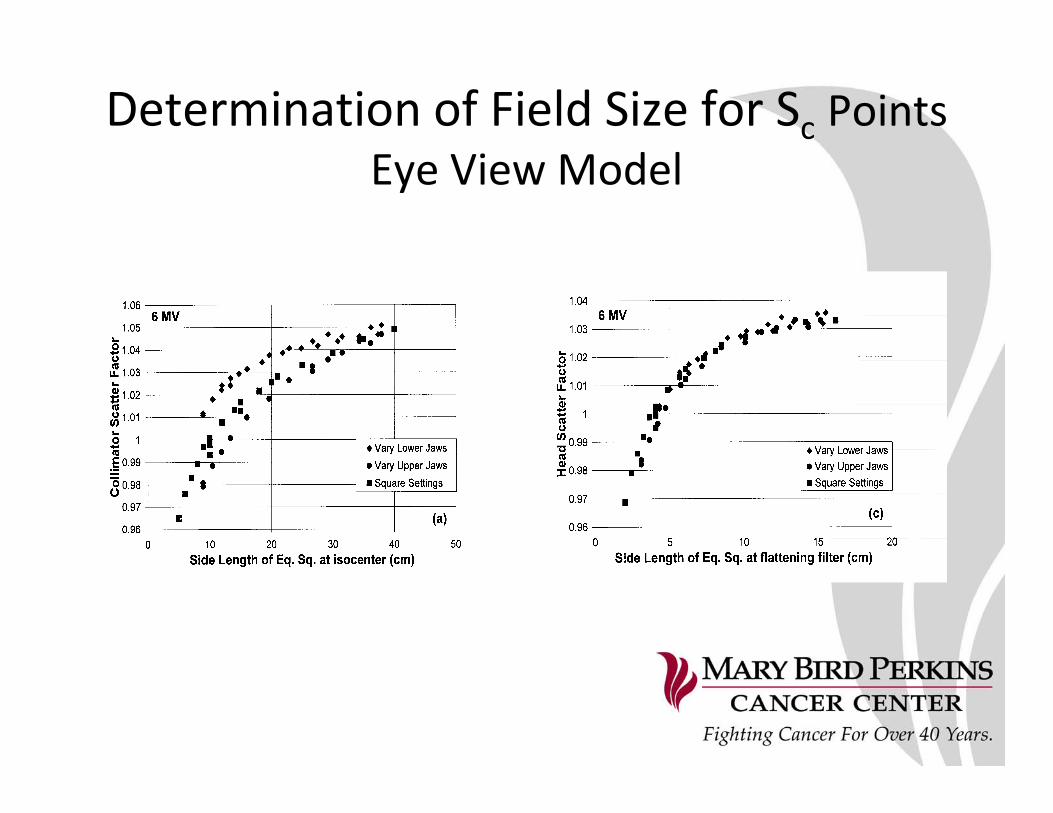
Determination of Field Size for ScSources of Head Scatter
• Backscatter to monitor chamber
• Head Scatter• Adjustable Collimators• Flattening Filter
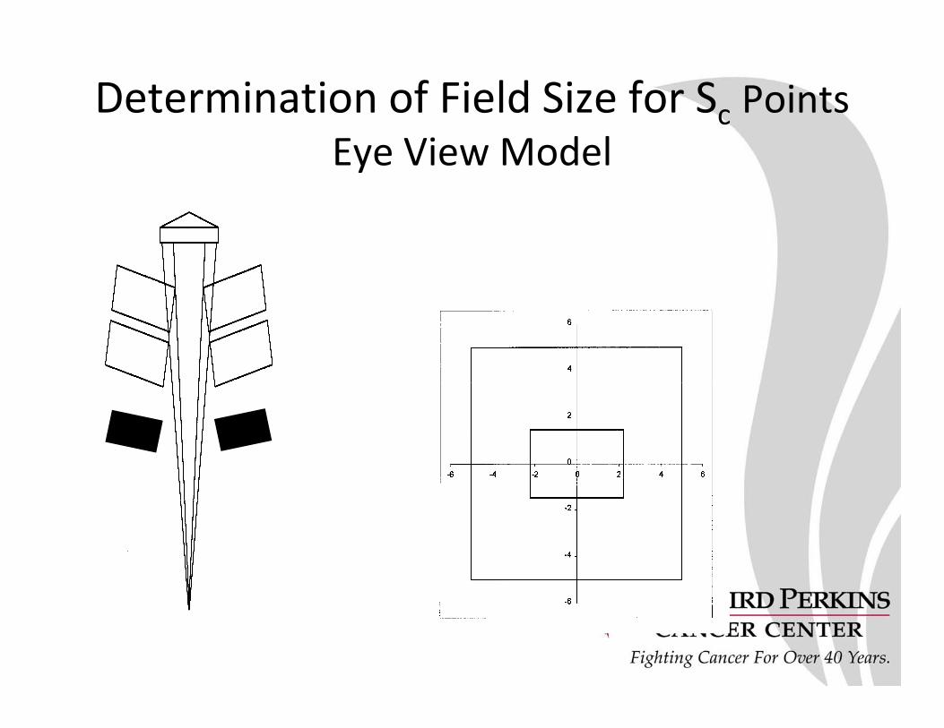
Determination of Field Size for Sc Points Eye View Model
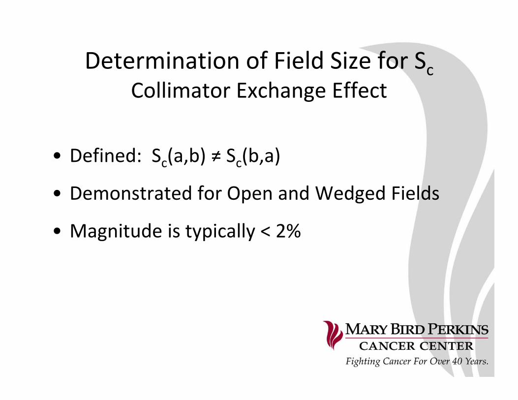
Determination of Field Size for ScCollimator Exchange Effect
• Defined: Sc(a,b) ≠ Sc(b,a)
• Demonstrated for Open and Wedged Fields
• Magnitude is typically < 2%
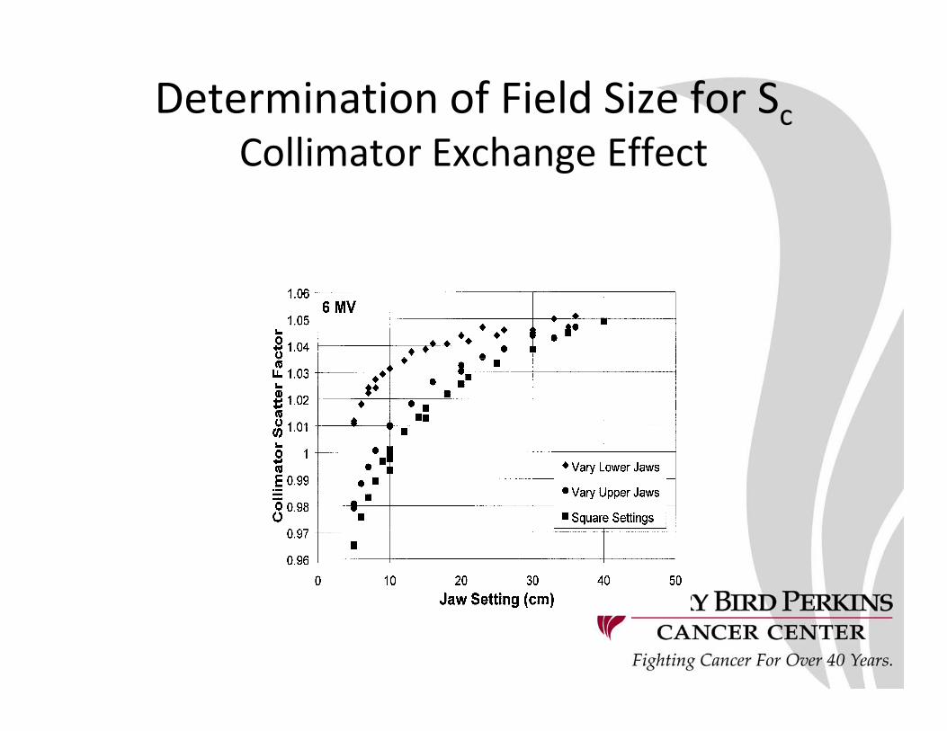
Determination of Field Size for ScCollimator Exchange Effect
Determination of Field Size for Sc Points Eye View Model
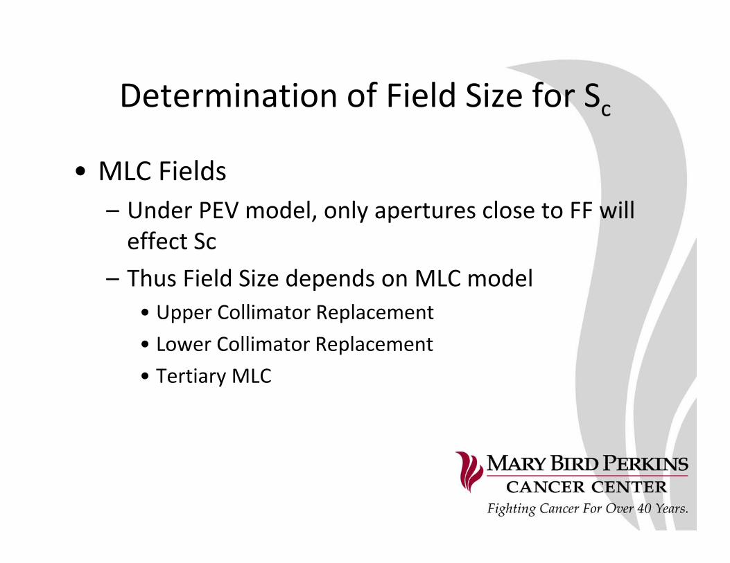
Determination of Field Size for Sc
• MLC Fields– Under PEV model, only apertures close to FF will effect Sc
– Thus Field Size depends on MLC model• Upper Collimator Replacement• Lower Collimator Replacement• Tertiary MLC
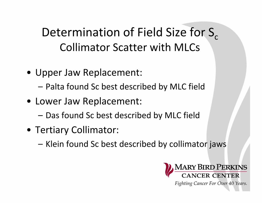
Determination of Field Size for ScCollimator Scatter with MLCs
• Upper Jaw Replacement:– Palta found Sc best described by MLC field
• Lower Jaw Replacement:– Das found Sc best described by MLC field
• Tertiary Collimator:– Klein found Sc best described by collimator jaws
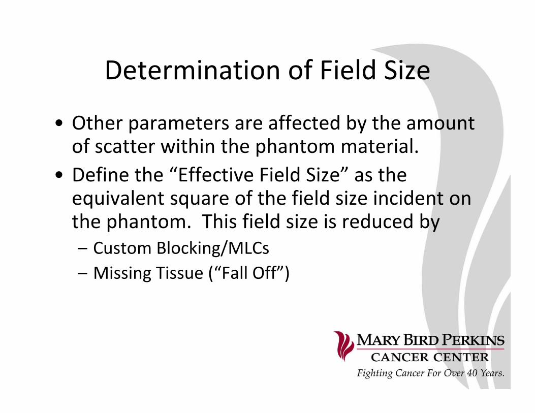
Determination of Field Size
• Other parameters are affected by the amount of scatter within the phantom material.
• Define the “Effective Field Size” as the equivalent square of the field size incident on the phantom. This field size is reduced by– Custom Blocking/MLCs– Missing Tissue (“Fall Off”)
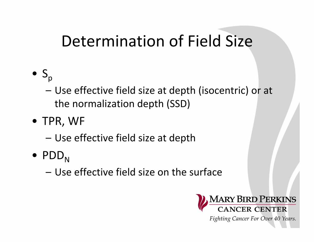
Determination of Field Size
• Sp– Use effective field size at depth (isocentric) or at the normalization depth (SSD)
• TPR, WF– Use effective field size at depth
• PDDN
– Use effective field size on the surface

For Photon Beams, the depth of normalization is:
0%
0%
0%
0%
0%
10
1. 10 cm2. dm3. dref4. Maximum dm < d0 < 10 cm5. Maximum dm < d0

For Photon Beams, the depth of normalization is:
5. Maximum dm < d0
Reference: AAPM Task Group 71 Report
The equivalent square for irregular fields may be approximated by:
0%
0%
0%
0%
0%
10
1. Equivalent area method2. 4A/P method, where A, P are the area, perimeter
of the irregular field3. 4A/P method, where A, P are the area, perimeter
of an equivalent rectangle to the irregular field4. PEV model for non‐tertiary MLC fields5. PEV model for all fields
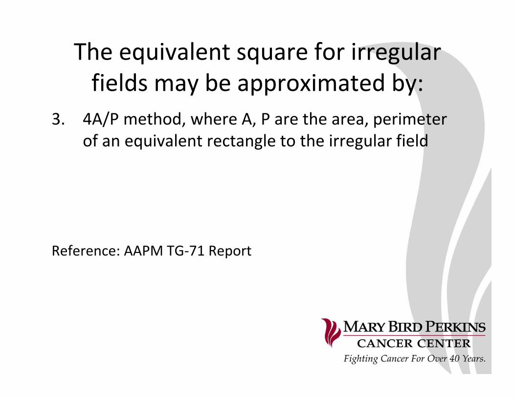
The equivalent square for irregular fields may be approximated by:
3. 4A/P method, where A, P are the area, perimeter of an equivalent rectangle to the irregular field
Reference: AAPM TG‐71 Report
Determination of DepthUse of Heterogeneity Corrections
• Not universally used• Importance of physician awareness• Two possible methods for manual calculations– Ratio of TAR (RTAR) method– Power law TAR (“Batho Method”)
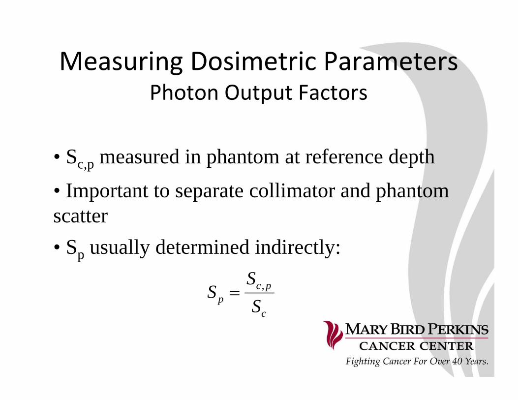
Measuring Dosimetric ParametersPhoton Output Factors
c
pcp S
SS ,=
• Sc,p measured in phantom at reference depth• Important to separate collimator and phantom scatter • Sp usually determined indirectly:
Measuring Dosimetric ParametersPhoton Output Factors
• Sc measured in air at reference depth. • Traditionally, measured with buildup cap• Larger do will require mini-phantoms
• Should avoid scatter from surrounding structures (support stands, floor, wall)
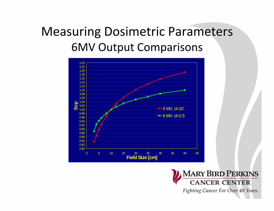
Measuring Dosimetric Parameters6MV Output Comparisons
0.800.820.840.860.880.900.920.940.960.981.001.021.041.061.081.101.121.141.161.181.201.221.24
0 5 10 15 20 25 30 35 40 45Field Size [cm]
Scp
6 MV, d=106 MV, d=1.5
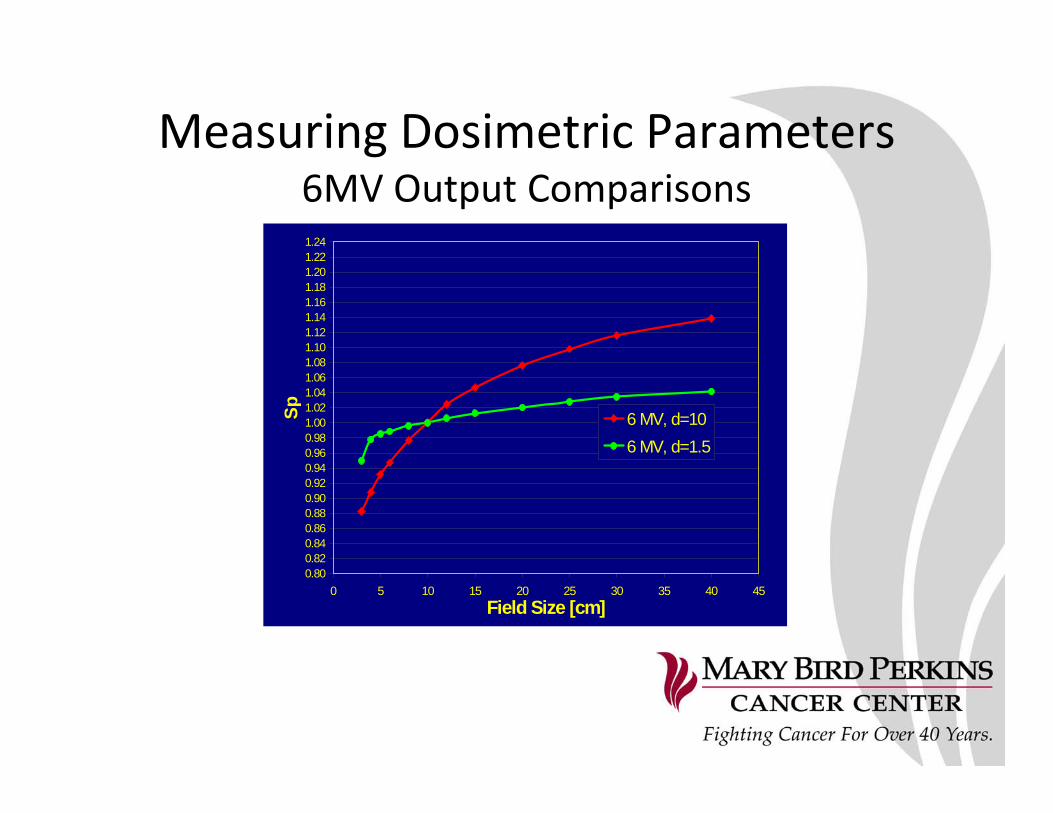
Measuring Dosimetric Parameters6MV Output Comparisons
0.800.820.840.860.880.900.920.940.960.981.001.021.041.061.081.101.121.141.161.181.201.221.24
0 5 10 15 20 25 30 35 40 45Field Size [cm]
Sp 6 MV, d=106 MV, d=1.5
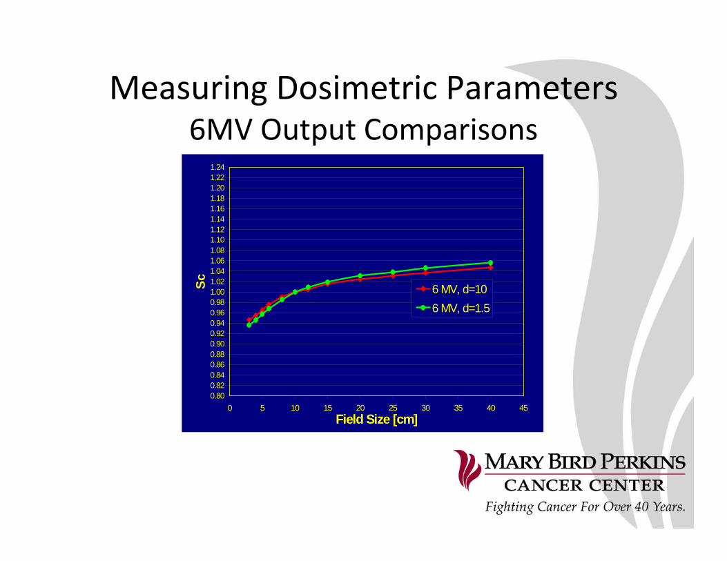
Measuring Dosimetric Parameters6MV Output Comparisons
0.800.820.840.860.880.900.920.940.960.981.001.021.041.061.081.101.121.141.161.181.201.221.24
0 5 10 15 20 25 30 35 40 45Field Size [cm]
Sc 6 MV, d=106 MV, d=1.5
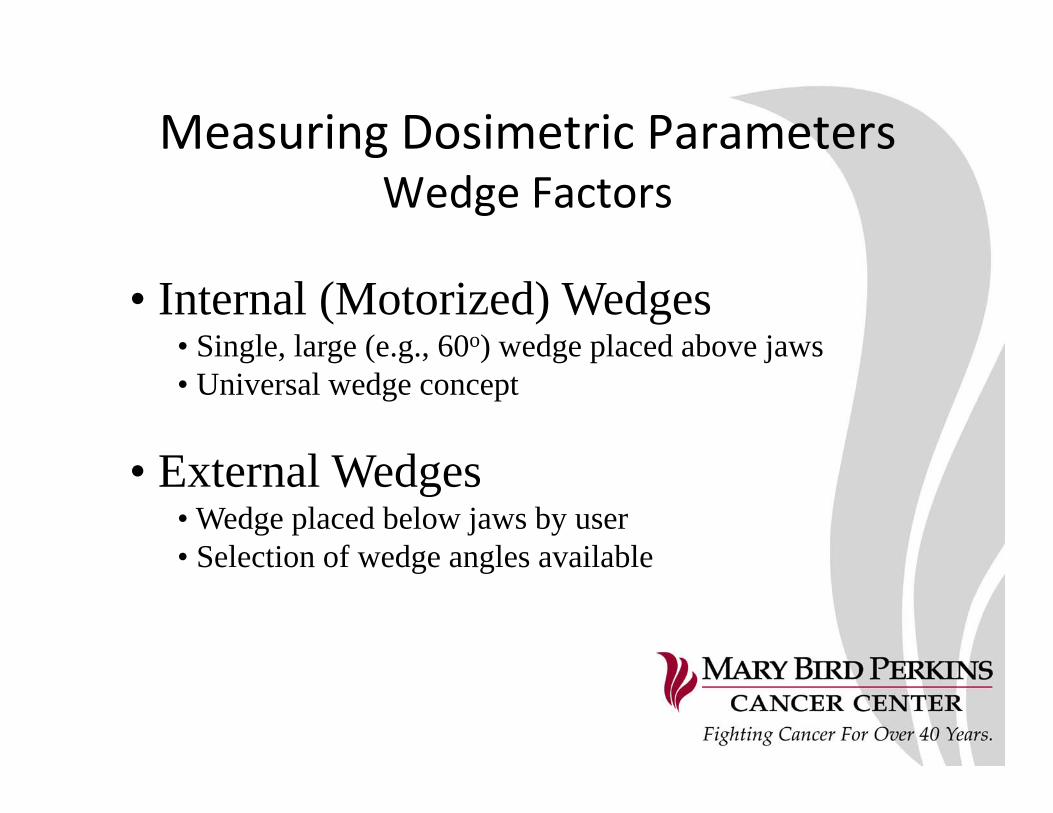
Measuring Dosimetric ParametersWedge Factors
• Internal (Motorized) Wedges• Single, large (e.g., 60o) wedge placed above jaws• Universal wedge concept
• External Wedges• Wedge placed below jaws by user• Selection of wedge angles available
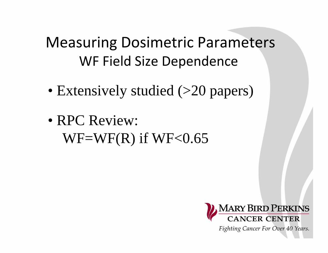
Measuring Dosimetric ParametersWF Field Size Dependence
• Extensively studied (>20 papers)
• RPC Review: WF=WF(R) if WF<0.65

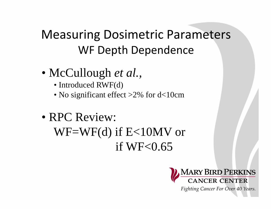
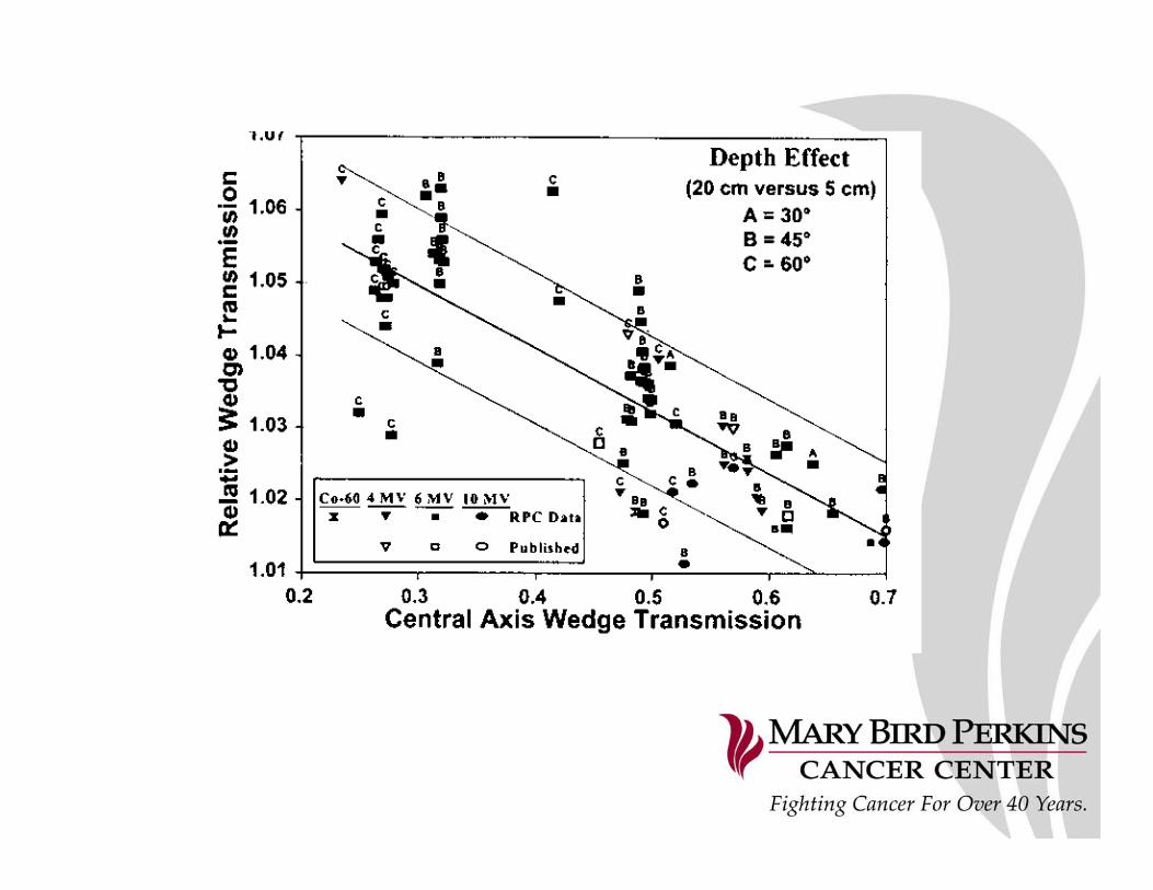
Measuring Dosimetric ParametersWF Depth Dependence
• McCullough et al.,• Introduced RWF(d)• No significant effect >2% for d<10cm
• RPC Review: WF=WF(d) if E<10MV or
if WF<0.65

Determining Dosimetric ParametersFilterless Wedge Factors
• EDW Factors– Direct Inspection of Final STT– Use of Normalized Golden STT– Analytic Equations
• VW Factors– Very close to unity for all Wedge Angles, Field Sizes
– Exponential Off‐Axis Relationship

Determining Dosimetric ParametersEDW Factors
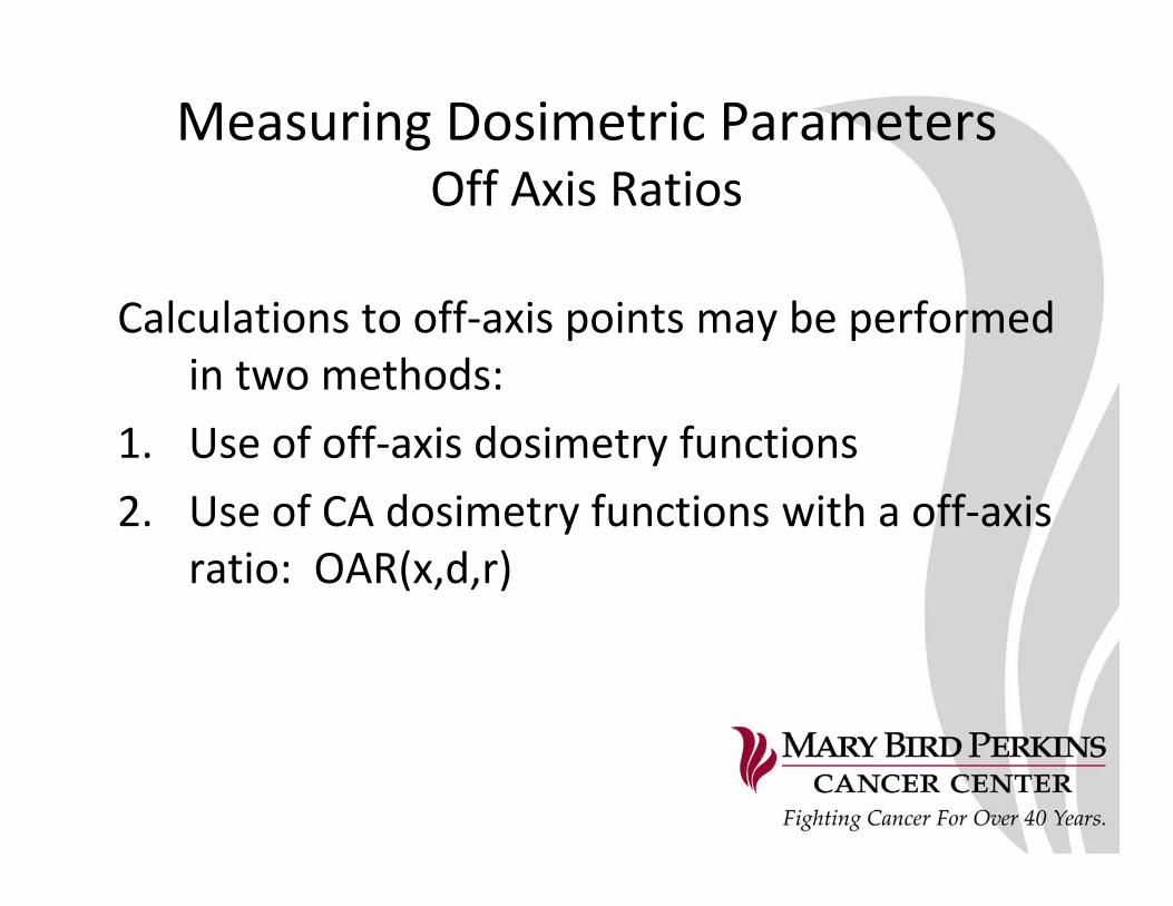
Measuring Dosimetric ParametersOff Axis Ratios
Calculations to off‐axis points may be performed in two methods:
1. Use of off‐axis dosimetry functions2. Use of CA dosimetry functions with a off‐axis
ratio: OAR(x,d,r)
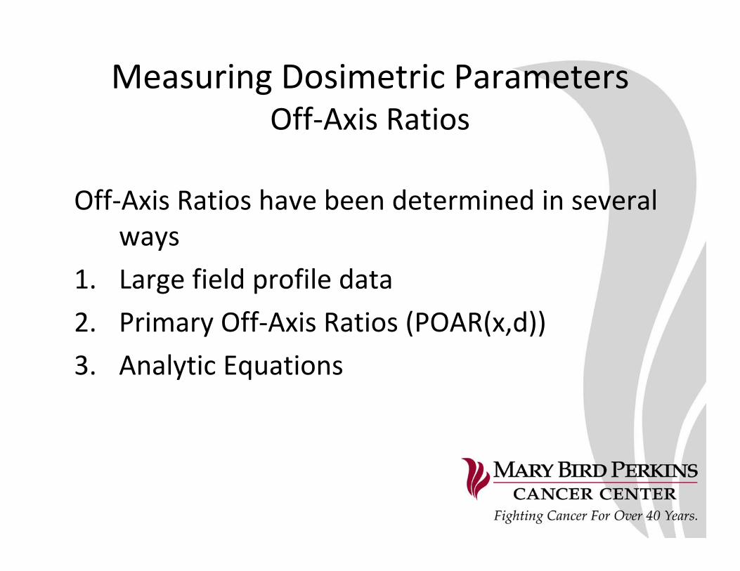
Measuring Dosimetric ParametersOff‐Axis Ratios
Off‐Axis Ratios have been determined in several ways
1. Large field profile data2. Primary Off‐Axis Ratios (POAR(x,d))3. Analytic Equations
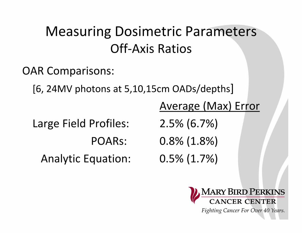
Measuring Dosimetric ParametersOff‐Axis Ratios
OAR Comparisons:[6, 24MV photons at 5,10,15cm OADs/depths]
Average (Max) ErrorLarge Field Profiles: 2.5% (6.7%)
POARs: 0.8% (1.8%)Analytic Equation: 0.5% (1.7%)

In MU calculations, wedge factors are
0%
0%
0%
0%
0%
10
1. Field size and depth dependent if WF<0.652. Always larger for physical wedges3. Defined at d = 10 cm4. Defined at d = dm5. Field size dependent only for internal
wedges
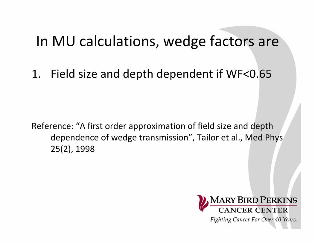
In MU calculations, wedge factors are
1. Field size and depth dependent if WF<0.65
Reference: “A first order approximation of field size and depth dependence of wedge transmission”, Tailor et al., Med Phys 25(2), 1998
Outline
I. IntroductionII. Photon Calculations
III. Electron Calculations
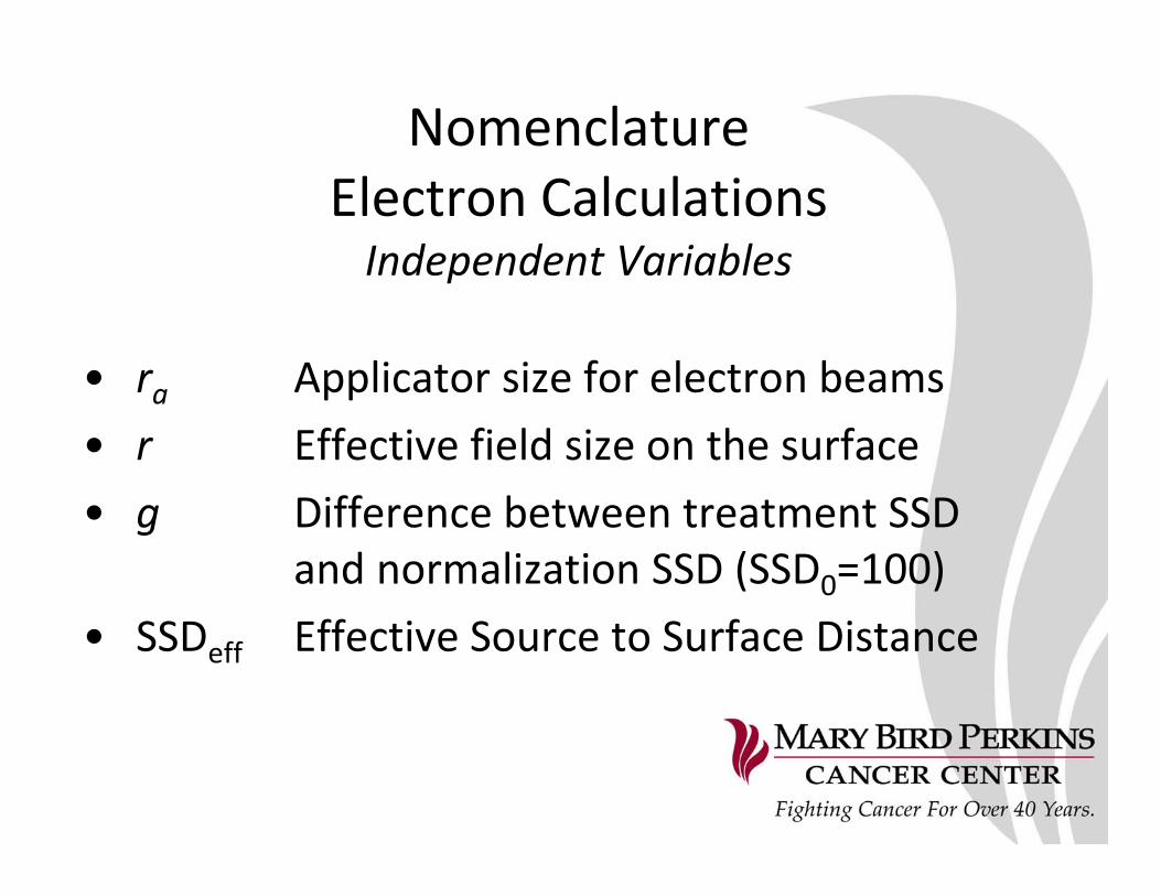
NomenclatureElectron CalculationsIndependent Variables
• ra Applicator size for electron beams• r Effective field size on the surface• g Difference between treatment SSD
and normalization SSD (SSD0=100) • SSDeff Effective Source to Surface Distance

NomenclatureElectron Calculations
Dependent Variables
• fair Air gap correction factor• Se Electron Output Factor
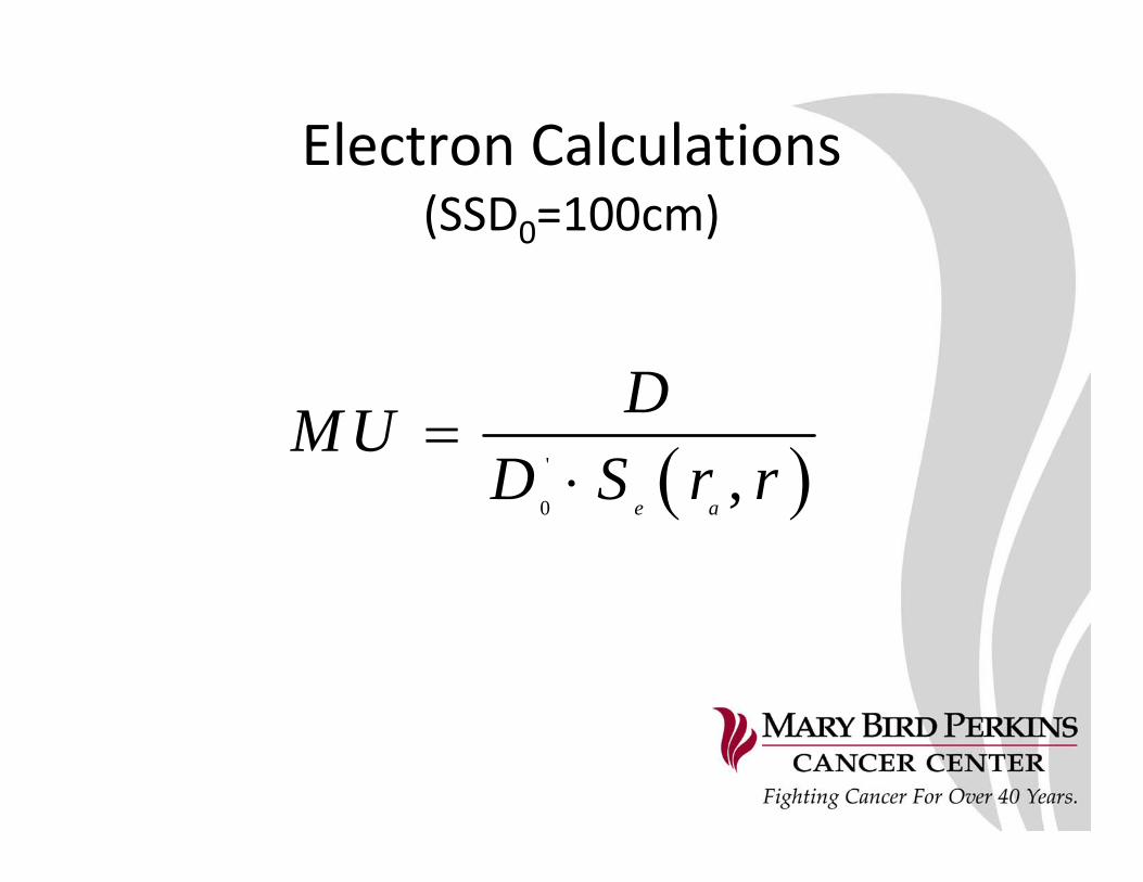
Electron Calculations(SSD0=100cm)
( )'
0,
e a
DM UD S r r
=⋅
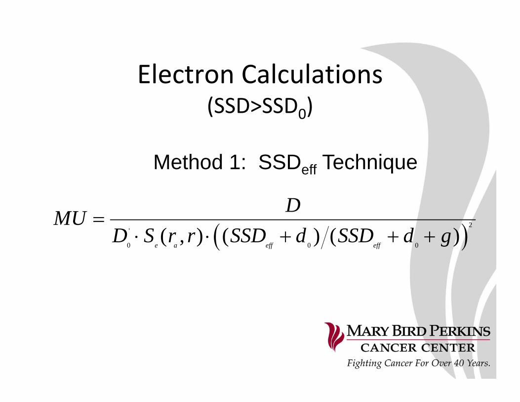
Electron Calculations(SSD>SSD0)
( )2'
0 0 0( , ) ( ) ( )
e a eff eff
DMUD S r r SSD d SSD d g
=⋅ ⋅ + + +
Method 1: SSDeff Technique
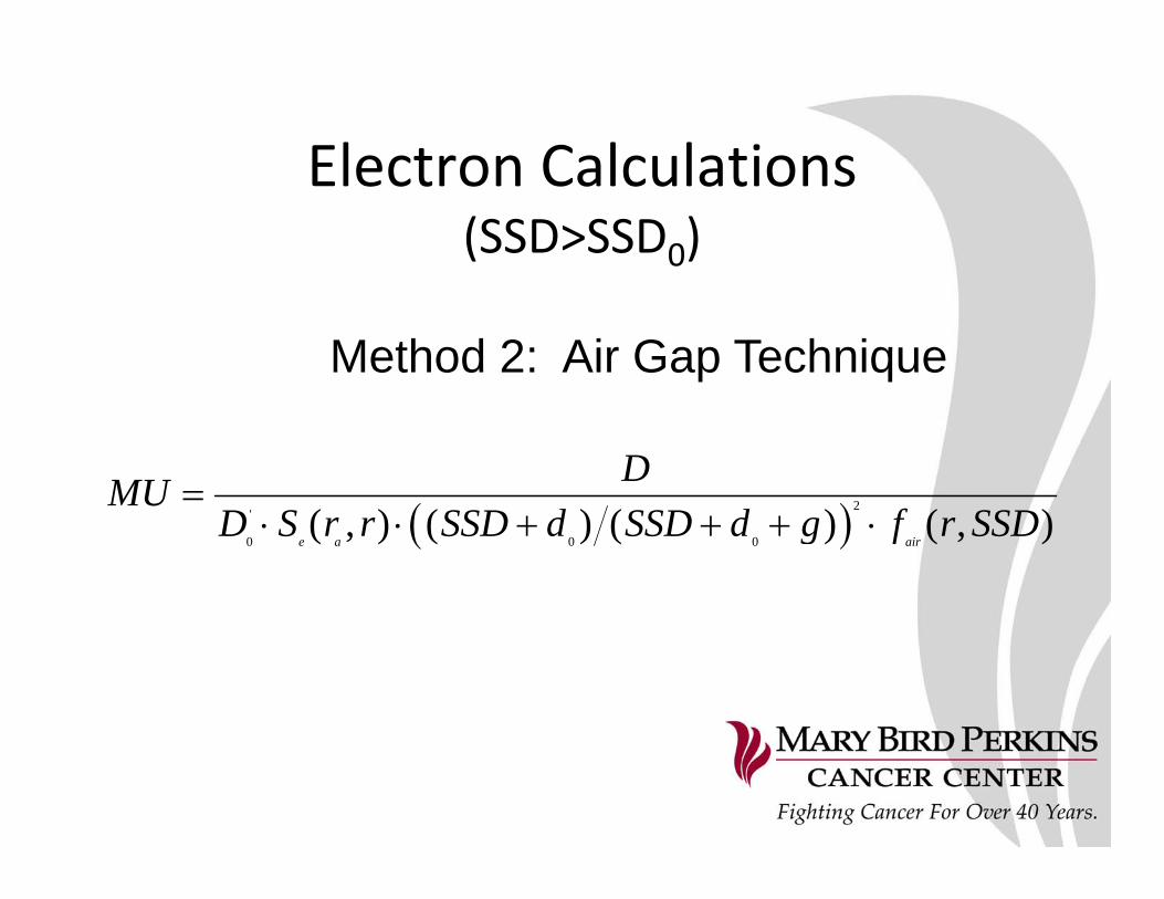
Electron Calculations(SSD>SSD0)
Method 2: Air Gap Technique
( )2'
0 0 0( , ) ( ) ( ) ( , )
e a air
DMUD S r r SSD d SSD d g f r SSD
=⋅ ⋅ + + + ⋅
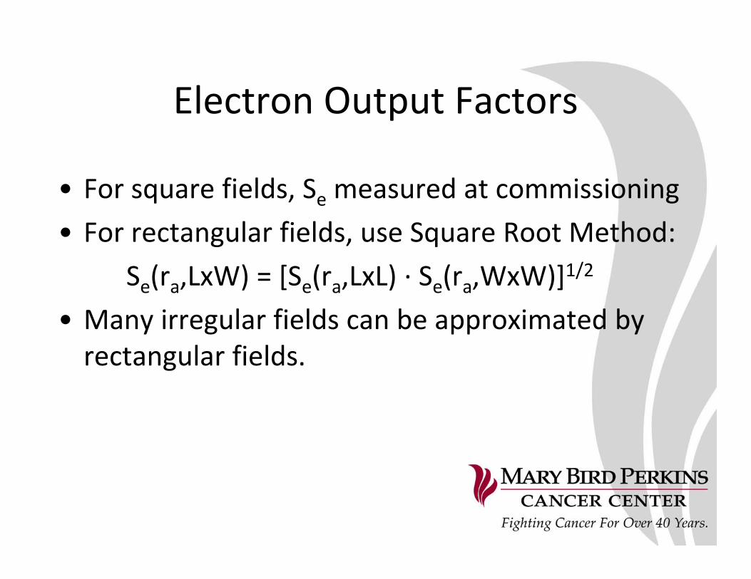
Electron Output Factors
• For square fields, Se measured at commissioning• For rectangular fields, use Square Root Method:
Se(ra,LxW) = [Se(ra,LxL) ∙ Se(ra,WxW)]1/2
• Many irregular fields can be approximated by rectangular fields.
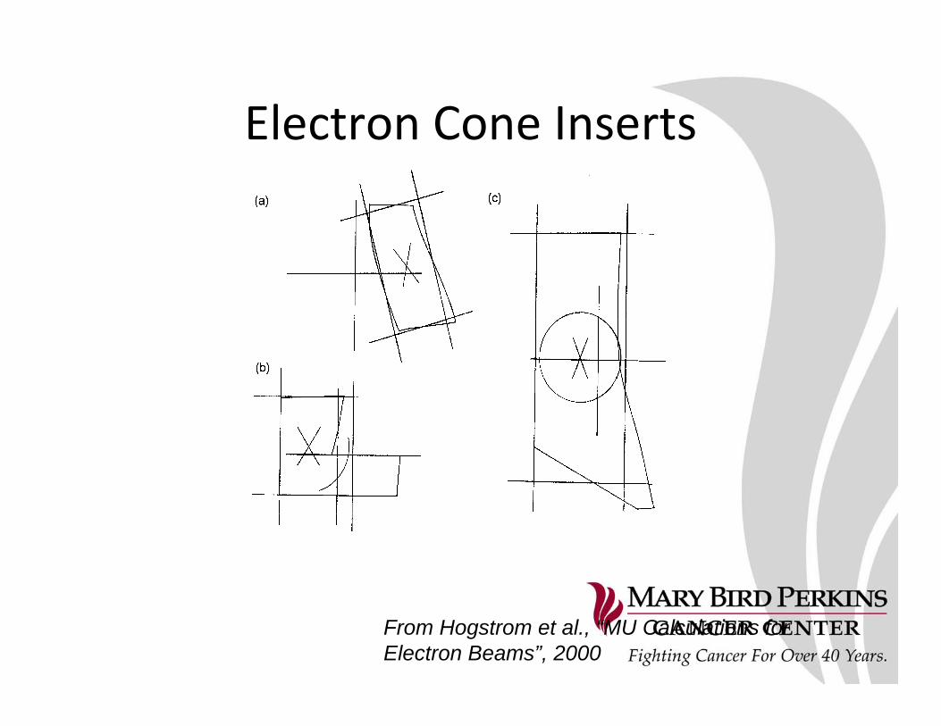
Electron Cone Inserts
From Hogstrom et al., “MU Calculations for Electron Beams”, 2000
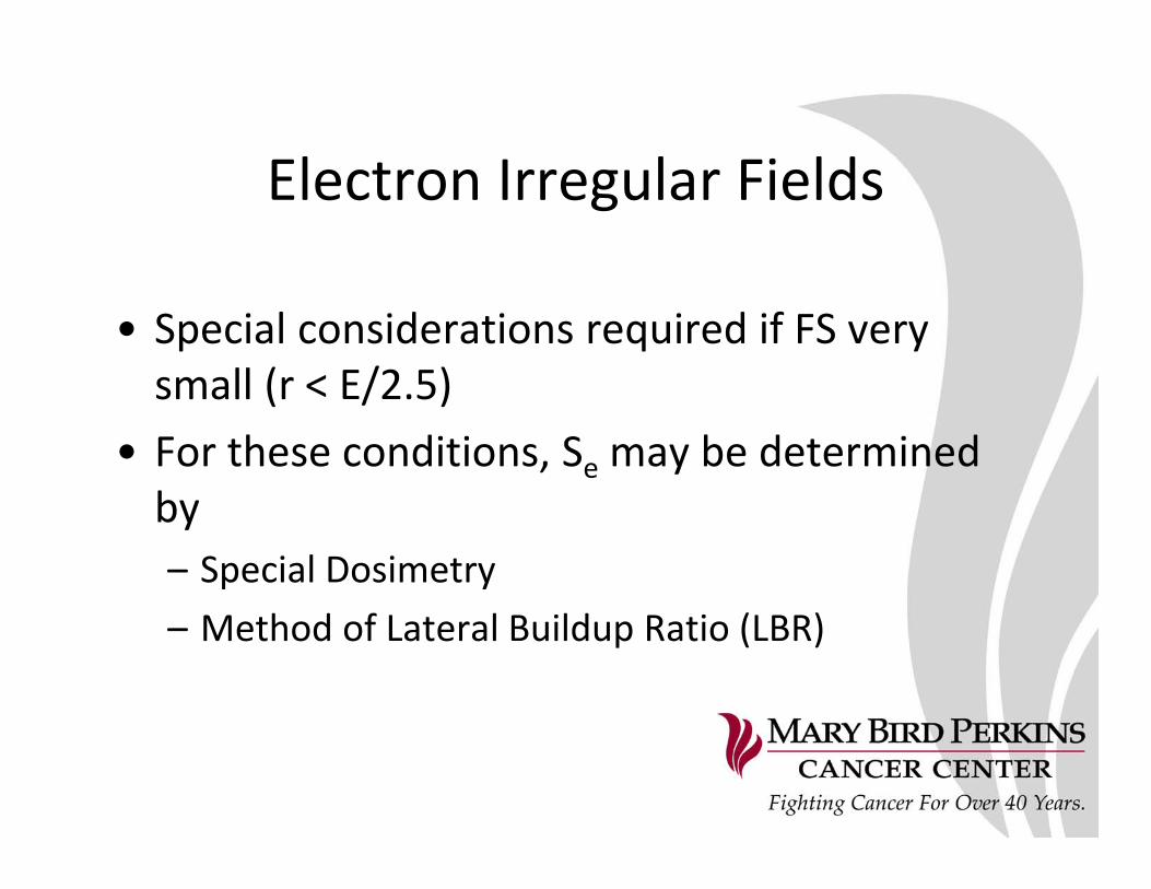
Electron Irregular Fields
• Special considerations required if FS very small (r < E/2.5)
• For these conditions, Se may be determined by– Special Dosimetry– Method of Lateral Buildup Ratio (LBR)

ElectronExtended SSD Calculations
• Many treatment geometries require extended SSDs
• The Air Gap Factormay be determined – Using inverse square correction with virtual SSD
• requires air gap scatter correction term
– Using inverse square correction with effective SSD
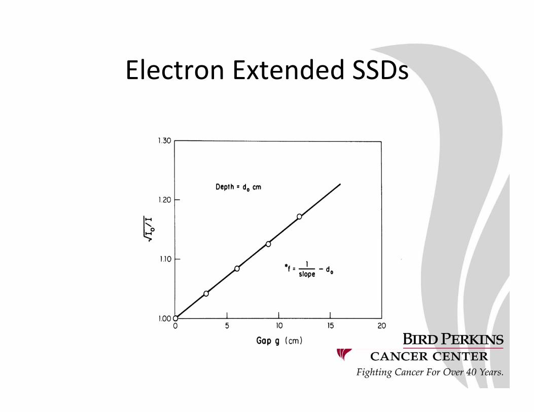
Electron Extended SSDs

Electron Extended SSDs
From Roback et al., “Effective SSD for Electron Beams …”, Med Phys 1995
For electron beams, the depth of normalization is
0%
0%
0%
0%
0%
10
1. 10 cm2. R100 for the given field3. R90 for the given field4. R100 for the open cone5. dref
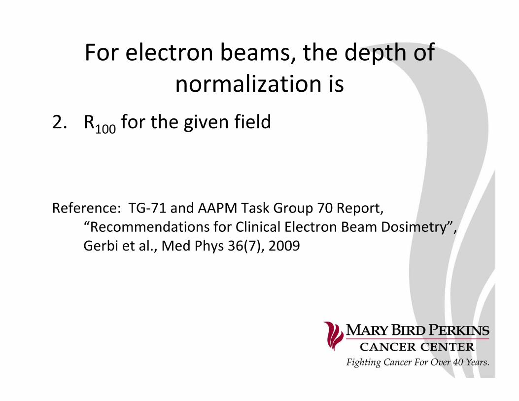
For electron beams, the depth of normalization is
2. R100 for the given field
Reference: TG‐71 and AAPM Task Group 70 Report, “Recommendations for Clinical Electron Beam Dosimetry”, Gerbi et al., Med Phys 36(7), 2009
Electron output factors at extended SSDs are:
0%
0%
0%
0%
0%
10
1. Independent of electron energy2. Calculated using the square root method3. Calculated either using effective SSDs or
air‐gap methods 4. Depend primarily on applicator field size5. Calculated using lateral build‐up ratios
Electron output factors at extended SSDs are
3. Calculated either using effective SSDs or air‐gap methods
Reference: TG‐71 and AAPM Task Group 70 Report, “Recommendations for Clinical Electron Beam Dosimetry”, Gerbi et al., Med Phys 36(7), 2009
Conclusions
• Task Group 71 of the RTC was formed to create a consistent nomenclature and formalism for MU Calculations
• For photon beams, TG71 recommends a normalization depth of 10cm, although the formalism is valid for (maximum) dm.
• For electron beams, TG71 allows for both effective SSD or Air Gap correction methods for extended SSD calculations


