UNIT-I

INTRODUCTION TO IMAGE PROCESSING

1.1 Introduction:

The digital image processing deals with developing a digital system that performs operations

on a digital image. An image is nothing more than a two dimensional signal. It is defined by

the mathematical function f(x,y) where x and y are the two co-ordinates horizontally and

vertically and the amplitude of f at any pair of coordinate (x, y) is called the intensity or gray

level of the image at that point. When x, y and the amplitude values of f are all finite discrete

quantities, we call the image a digital image. The field of image digital image processing

refers to the processing of digital image by means of a digital computer. A digital image is

composed of a finite number of elements, each of which has a particular location and values

of these elements are referred to as picture elements, image elements, pels and pixels.

Motivation and Perspective:

Digital image processing deals with manipulation of digital images through a digital

computer. It is a subfield of signals and systems but focus particularly on images. DIP

focuses on developing a computer system that is able to perform processing on an image. The

input of that system is a digital image and the system process that image using efficient

algorithms, and gives an image as an output. The most common example is Adobe

Photoshop. It is one of the widely used application for processing digital images.

Applications:

Some of the major fields in which digital image processing is widely used are mentioned

below

(1) Gamma Ray Imaging- Nuclear medicine and astronomical observations.

(2) X-Ray imaging – X-rays of body.

(3) Ultraviolet Band –Lithography, industrial inspection, microscopy, lasers.

(4) Visual And Infrared Band – Remote sensing.

(5) Microwave Band – Radar imaging.

1.2 Components of Image processing System:

i) Image Sensors: With reference to sensing, two elements are required to acquire digital

image. The first is a physical device that is sensitive to the energy radiated by the object we

wish to image and second is specialized image processing hardware.

ii) Specialize image processing hardware: It consists of the digitizer just mentioned, plus

hardware that performs other primitive operations such as an arithmetic logic unit, which

performs arithmetic such addition and subtraction and logical operations in parallel on images

iii) Computer: It is a general purpose computer and can range from a PC to a supercomputer

depending on the application. In dedicated applications, sometimes specially designed

computer are used to achieve a required level of performance

iv) Software: It consists of specialized modules that perform specific tasks a well designed

package also includes capability for the user to write code, as a minimum, utilizes the

specialized module. More sophisticated software packages allow the integration of these

modules.

v) Mass storage: This capability is a must in image processing applications. An image of

size 1024 x1024 pixels, in which the intensity of each pixel is an 8- bit quantity requires one

Megabytes of storage space if the image is not compressed .Image processing applications

falls into three principal categories of storage

i) Short term storage for use during processing

ii) On line storage for relatively fast retrieval

iii) Archival storage such as magnetic tapes and disks

vi) Image display: Image displays in use today are mainly color TV monitors. These

monitors are driven by the outputs of image and graphics displays cards that are an integral

part of computer system.

vii) Hardcopy devices: The devices for recording image includes laser printers, film

cameras, heat sensitive devices inkjet units and digital units such as optical and CD ROM

disk. Films provide the highest possible resolution, but paper is the obvious medium of

choice for written applications.

viii) Networking: It is almost a default function in any computer system in use today because

of the large amount of data inherent in image processing applications. The key consideration

in image transmission bandwidth.

1.3 Elements of Visual Spectrum:

(i) Structure of Human eye:

The eye is nearly a sphere with average approximately 20 mm diameter. The eye is enclosed

with three membranes

a) The cornea and sclera - it is a tough, transparent tissue that covers the anterior surface of

the eye. Rest of the optic globe is covered by the sclera

b) The choroid – It contains a network of blood vessels that serve as the major source of

nutrition to the eyes. It helps to reduce extraneous light entering in the eye It has two parts

(1) Iris Diaphragms- it contracts or expands to control the amount of light that enters

the eyes

(2) Ciliary body

(c) Retina – it is innermost membrane of the eye. When the eye is properly focused, light

from an object outside the eye is imaged on the retina. There are various light receptors over

the surface of the retina The two major classes of the receptors are-

1) cones- it is in the number about 6 to 7 million. These are located in the central portion of

the retina called the fovea. These are highly sensitive to color. Human can resolve fine details

with these cones because each one is connected to its own nerve end. Cone vision is called

photonic or bright light vision.

2) Rods – these are very much in number from 75 to 150 million and are distributed over the

entire retinal surface. The large area of distribution and the fact that several roads are

connected to a single nerve give a general overall picture of the field of view. They are not

involved in the color vision and are sensitive to low level of illumination. Rod vision is called

is isotopic or dim light vision. The absent of reciprocators is called blind spot.

(ii) Image formation in the eye:

The major difference between the lens of the eye and an ordinary optical lens in that the

former is flexible. The shape of the lens of the eye is controlled by tension in the fiber of the

ciliary body. To focus on the distant object the controlling muscles allow the lens to become

thicker in order to focus on object near the eye it becomes relatively flattened. The distance

between the center of the lens and the retina is called the focal length and it varies from

17mm to 14mm as the refractive power of the lens increases from its minimum to its

maximum. When the eye focuses on an object farther away than about 3m.the lens exhibits

its lowest refractive power. When the eye focuses on a nearly object. The lens is most srongly

refractive. The retinal image is reflected primarily in the area of the fovea. Perception then

takes place by the relative excitation of light receptors, which transform radiant energy into

electrical impulses that are ultimately decoded by the brain.

(iii) Brightness adaption and discrimination:

Digital image are displayed as a discrete set of intensities. The range of light intensity levels

to which the human visual system can adopt is enormous- on the order of 1010

- from isotopic

threshold to the glare limit. Experimental evidences indicate that subjective brightness is a

logarithmic function of the light intensity incident on the eye.

The curve represents the range of intensities to which the visual system can adopt. But the

visual system cannot operate over such a dynamic range simultaneously. Rather, it is

accomplished by change in its overcall sensitivity called brightness adaptation. For any given

set of conditions, the current sensitivity level to which of the visual system is called

brightness adoption level , Ba in the curve. The small intersecting curve represents the range

of subjective brightness that the eye can perceive when adapted to this level. It is restricted at

level Bb , at and below which all stimuli are perceived as indistinguishable blacks. The upper

portion of the curve is not actually restricted. Whole simply raise the adaptation level higher

than Ba. The ability of the eye to discriminate between change in light intensity at any

specific adaptation level is also of considerable interest. Take a flat, uniformly illuminated

area large enough to occupy the entire field of view of the subject. It may be a diffuser such

as an opaque glass, that is illuminated from behind by a light source whose intensity, I can be

varied. To this field is added an increment of illumination ΔI in the form of a short duration

flash that appears as circle in the center of the uniformly illuminated field. If ΔI is not bright

enough, the subject cannot see any perceivable changes.

As ΔI gets stronger the subject may indicate of a perceived change. ΔIc is the increment of

illumination discernible 50% of the time with background illumination I. Now, ΔIc /I is

called the Weber ratio. Small value means that small percentage change in intensity is

discernible representing “good” brightness discrimination. Large value of Weber ratio means

large percentage change in intensity is required representing “poor brightness

discrimination”.

(iv) Optical Illusion:

In this the eye fills the non existing information or wrongly pervious geometrical properties

of objects.

1.4 Fundamental steps involved in Image processing:

There are two categories of the steps involved in the image processing –

(1) Methods whose outputs are input are images.

(2) Methods whose outputs are attributes extracted from those images.

i) Image acquisition: It could be as simple as being given an image that is already in digital

form. Generally the image acquisition stage involves processing such scaling.

ii) Image Enhancement: It is among the simplest and most appealing areas of digital image

processing. The idea behind this is to bring out details that are obscured or simply to

highlight certain features of interest in image. Image enhancement is a very subjective area of

image processing.

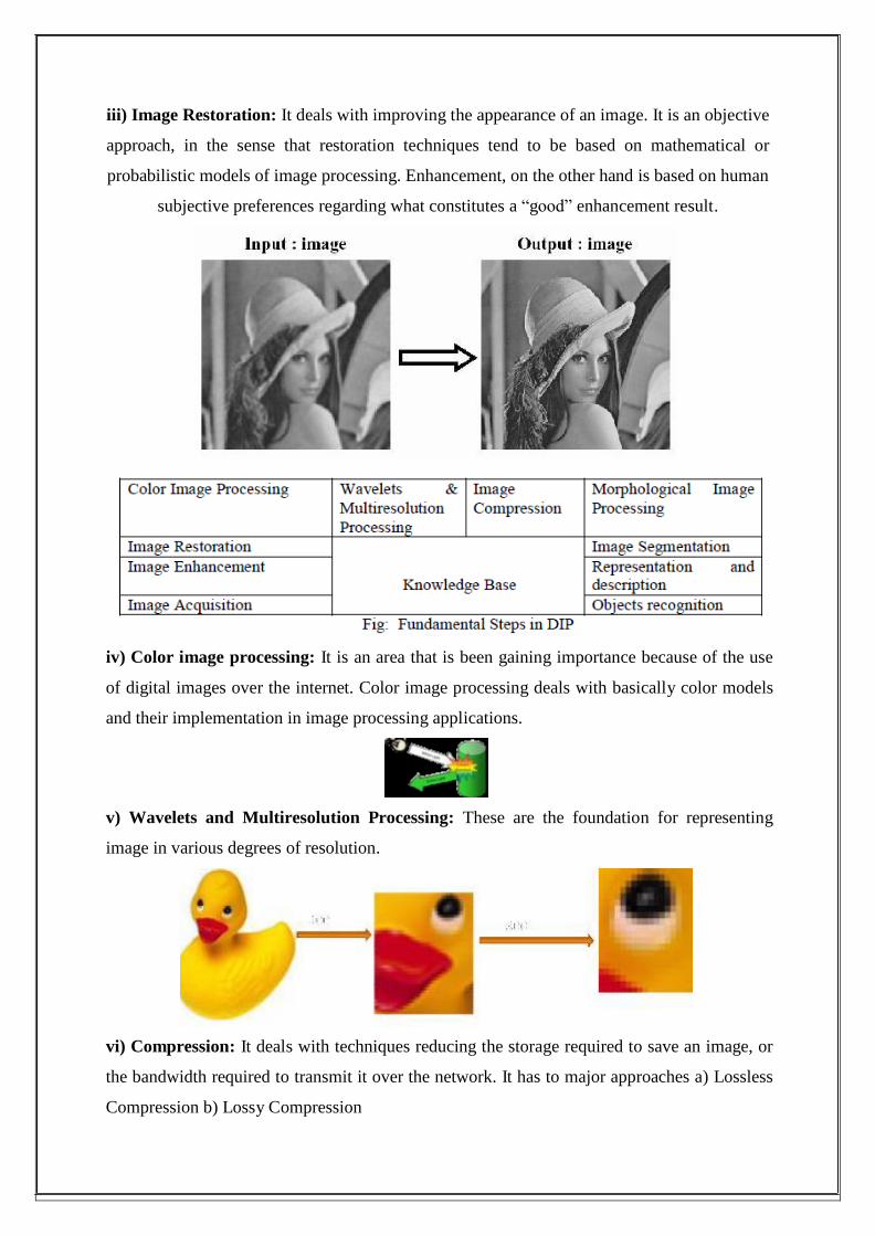
iii) Image Restoration: It deals with improving the appearance of an image. It is an objective

approach, in the sense that restoration techniques tend to be based on mathematical or

probabilistic models of image processing. Enhancement, on the other hand is based on human

subjective preferences regarding what constitutes a “good” enhancement result.

iv) Color image processing: It is an area that is been gaining importance because of the use

of digital images over the internet. Color image processing deals with basically color models

and their implementation in image processing applications.

v) Wavelets and Multiresolution Processing: These are the foundation for representing

image in various degrees of resolution.

vi) Compression: It deals with techniques reducing the storage required to save an image, or

the bandwidth required to transmit it over the network. It has to major approaches a) Lossless

Compression b) Lossy Compression

vii) Morphological processing: It deals with tools for extracting image components that are

useful in the representation and description of shape and boundary of objects. It is majorly

used in automated inspection applications.

viii) Representation and Description: It always follows the output of segmentation step that

is, raw pixel data, constituting either the boundary of an image or points in the region itself.

In either case converting the data to a form suitable for computer processing is necessary.

ix) Recognition: It is the process that assigns label to an object based on its descriptors. It is

the last step of image processing which use artificial intelligence of software.

Knowledge base:

Knowledge about a problem domain is coded into an image processing system in the form of

a knowledge base. This knowledge may be as simple as detailing regions of an image where

the information of the interest in known to be located. Thus limiting search that has to be

conducted in seeking the information. The knowledge base also can be quite complex such

interrelated list of all major possible defects in a materials inspection problems or an image

database containing high resolution satellite images of a region in connection with change

detection application.

1.5 A Simple Image Model:

An image is denoted by a two dimensional function of the form f{x, y}. The value or

amplitude of f at spatial coordinates {x,y} is a positive scalar quantity whose physical

meaning is determined by the source of the image. When an image is generated by a physical

process, its values are proportional to energy radiated by a physical source. As a

consequence, f(x,y) must be nonzero and finite; that is o<f(x,y) <co

The function f(x,y) may be characterized by two components-

(a) The amount of the source illumination incident on the scene being viewed.

(b) The amount of the source illumination reflected back by the objects in the scene

These are called illumination and reflectance components and are denoted by i (x,y) an r (x,y)

respectively.

The functions combine as a product to form f(x,y). We call the intensity of a monochrome

image at any coordinates (x,y) the gray level (l) of the image at that point l= f (x, y.)

L min ≤ l ≤ Lmax

Lmin is to be positive and Lmax must be finite

Lmin = imin rmin

Lmax = imax rmax

The interval [Lmin, Lmax] is called gray scale. Common practice is to shift this interval

numerically to the interval [0, L-l] where l=0 is considered black and l= L-1 is considered

white on the gray scale. All intermediate values are shades of gray of gray varying from black

to white.

1.6 Image Sampling And Quantization:

To create a digital image, we need to convert the continuous sensed data into digital from.

This involves two processes – sampling and quantization. An image may be continuous with

respect to the x and y coordinates and also in amplitude. To convert it into digital form we

have to sample the function in both coordinates and in amplitudes.

Digitalizing the coordinate values is called sampling.

Digitalizing the amplitude values is called quantization.

There is a continuous the image along the line segment AB.

To simple this function, we take equally spaced samples along line AB. The location of each

samples is given by a vertical tick back (mark) in the bottom part. The samples are shown as

block squares superimposed on function the set of these discrete locations gives the sampled

function.

In order to form a digital, the gray level values must also be converted (quantized) into

discrete quantities. So we divide the gray level scale into eight discrete levels ranging from

eight level values. The continuous gray levels are quantized simply by assigning one of the

eight discrete gray levels to each sample. The assignment it made depending on the vertical

proximity of a simple to a vertical tick mark.

Starting at the top of the image and covering out this procedure line by line produces a two

dimensional digital image.

1.7 Digital Image definition:

A digital image f(m,n) described in a 2D discrete space is derived from an analog image

f(x,y) in a 2D continuous space through a sampling process that is frequently referred to as

digitization. The mathematics of that sampling process will be described in subsequent

Chapters. For now we will look at some basic definitions associated with the digital image.

The effect of digitization is shown in figure.

The 2D continuous image f(x,y) is divided into N rows and M columns. The intersection of a

row and a column is termed a pixel. The value assigned to the integer coordinates (m,n) with

m=0,1,2..N-1 and n=0,1,2…N-1 is f(m,n). In fact, in most cases, is actually a function of

many variables including depth, color and time (t).

There are three types of computerized processes in the processing of image

1) Low level process -these involve primitive operations such as image processing to reduce

noise, contrast enhancement and image sharpening. These kind of processes are characterized

by fact the both inputs and output are images.

2) Mid level image processing - it involves tasks like segmentation, description of those

objects to reduce them to a form suitable for computer processing, and classification of

individual objects. The inputs to the process are generally images but outputs are attributes

extracted from images.

3) High level processing – It involves “making sense” of an ensemble of recognized objects,

as in image analysis, and performing the cognitive functions normally associated with vision.

1.8 Representing Digital Images:

The result of sampling and quantization is matrix of real numbers. Assume that an image

f(x,y) is sampled so that the resulting digital image has M rows and N Columns. The values

of the coordinates (x,y) now become discrete quantities thus the value of the coordinates at

orgin become 9X,y) =(o,o) The next Coordinates value along the first signify the iamge along

the first row. it does not mean that these are the actual values of physical coordinates when

the image was sampled.

Thus the right side of the matrix represents a digital element, pixel or pel. The matrix can be

represented in the following form as well. The sampling process may be viewed as

partitioning the xy plane into a grid with the coordinates of the center of each grid being a

pair of elements from the Cartesian products Z2 which is the set of all ordered pair of

elements (Zi, Zj) with Zi and Zj being integers from Z. Hence f(x,y) is a digital image if gray

level (that is, a real number from the set of real number R) to each distinct pair of coordinates

(x,y). This functional assignment is the quantization process. If the gray levels are also

integers, Z replaces R, the and a digital image become a 2D function whose coordinates and

she amplitude value are integers. Due to processing storage and hardware consideration, the

number gray levels typically is an integer power of 2.

L=2k

Then, the number, b, of bites required to store a digital image is B=M *N* k

When M=N, the equation become b=N2*k

When an image can have 2k gray levels, it is referred to as “k- bit”. An image with 256

possible gray levels is called an “8- bit image” (256=28).

1.9 Spatial and Gray level resolution:

Spatial resolution is the smallest discernible details are an image. Suppose a chart can be

constructed with vertical lines of width w with the space between the also having width W, so

a line pair consists of one such line and its adjacent space thus. The width of the line pair is

2w and there is 1/2w line pair per unit distance resolution is simply the smallest number of

discernible line pair unit distance.

Gray levels resolution refers to smallest discernible change in gray levels. Measuring

discernible change in gray levels is a highly subjective process reducing the number of bits R

while repairing the spatial resolution constant creates the problem of false contouring.

It is caused by the use of an insufficient number of gray levels on the smooth areas of the

digital image . It is called so because the rides resemble top graphics contours in a map. It is

generally quite visible in image displayed using 16 or less uniformly spaced gray levels.

1.10 Relationship between pixels:

(i) Neighbor of a pixel:

A pixel p at coordinate (x,y) has four horizontal and vertical neighbor whose coordinate can

be given by

(x+1, y) (X-1,y) (X ,y + 1) (X, y-1)

This set of pixel called the 4-neighbours of p is denoted by n4(p) ,Each pixel is a unit distance

from (x,y) and some of the neighbors of P lie outside the digital image of (x,y) is on the

border if the image . The four diagonal neighbor of P have coordinated

(x+1,y+1),(x+1,y+1),(x-1,y+1),(x-1,y-1)

And are deported by nd (p) .these points, together with the 4-neighbours are called 8 –

neighbors of P denoted by ns(p).

(ii) Adjacency:

Let v be the set of gray –level values used to define adjacency, in a binary image, v={1} if

we are reference to adjacency of pixel with value. Three types of adjacency

4- Adjacency – two pixel P and Q with value from V are 4 –adjacency if A is in the set n4(P)

8- Adjacency – two pixel P and Q with value from V are 8 –adjacency if A is in the set n8(P)

M-adjacency –two pixel P and Q with value from V are m – adjacency if

(i) Q is in n4 (p) or

(ii)Q is in nd (q) and the set N4(p) U N4(q) has no pixel whose values are from V

(iii) Distance measures:

For pixel p,q and z with coordinate (x.y) ,(s,t) and (v,w) respectively D is a distance function

or metric if

D [p.q] ≥ O {D[p.q] = O iff p=q}

D [p.q] = D [p.q] and

D [p.q] ≥ O {D[p.q]+D(q,z)

The Education Distance between p and is defined as

De (p,q) = Iy – t I

The D4 Education Distance between p and is defined as

De (p,q) = Iy – t I

1.11 Image sensing and Acquisition:

The types of images in which we are interested are generated by the combination of an

Fig:Single Image sensor

Fig: Line Sensor

Fig: Array sensor

“illumination” source and the reflection or absorption of energy from that source by the

elements of the “scene” being imaged. We enclose illumination and scene in quotes to

emphasize the fact that they are considerably more general than the familiar situation in

which a visible light source illuminates a common everyday 3-D (three-dimensional) scene.

For example, the illumination may originate from a source of electromagnetic energy such as

radar, infrared, or X-ray energy. But, as noted earlier, it could originate from less traditional

sources, such as ultrasound or even a computer-generated illumination pattern. Similarly, the

scene elements could be familiar objects, but they can just as easily be molecules, buried rock

formations, or a human brain. We could even image a source, such as acquiring images of the

sun. Depending on the nature of the source, illumination energy is reflected from, or

transmitted through, objects. An example in the first category is light reflected from a planar

surface. An example in the second category is when X-rays pass through a patient‟s body for

thepurpose of generating a diagnostic X-ray film. In some applications, the reflected or

transmitted energy is focused onto a photo converter (e.g., a phosphor screen), which

converts the energy into visible light. Electron microscopy and some applications of gamma

imaging use this approach. The idea is simple: Incoming energy is transformed into a voltage

by the combination of input electrical power and sensor material that is responsive to the

particular type of energy being detected. The output voltage waveform is the response of the

sensor(s), and a digital quantity is obtained from each sensor by digitizing its response. In this

section, we look at the principal modalities for image sensing and generation.

(i)Image Acquisition using a Single sensor:

The components of a single sensor. Perhaps the most familiar sensor of this type is the

photodiode, which is constructed of silicon materials and whose output voltage waveform is

proportional to light. The use of a filter in front of a sensor improves selectivity. For example,

a green (pass) filter in front of a light sensor favors light in the green band of the color

spectrum. As a consequence, the sensor output will be stronger for green light than for other

components in the visible spectrum.

In order to generate a 2-D image using a single sensor, there has to be relative displacements

in both the x- and y-directions between the sensor and the area to be imaged. Figure shows an

arrangement used in high-precision scanning, where a film negative is mounted onto a drum

whose mechanical rotation provides displacement in one dimension. The single sensor is

mounted on a lead screw that provides motion in the perpendicular direction. Since

mechanical motion can be controlled with high precision, this method is an inexpensive (but

slow) way to obtain high-resolution images. Other similar mechanical arrangements use a flat

bed, with the sensor moving in two linear directions. These types of mechanical digitizers

sometimes are referred to as microdensitometers.

(ii)Image Acquisition using a Sensor strips:

A geometry that is used much more frequently than single sensors consists of an in-line

arrangement of sensors in the form of a sensor strip, shows. The strip provides imaging

elements in one direction. Motion perpendicular to the strip provides imaging in the other

direction. This is the type of arrangement used in most flat bed scanners. Sensing devices

with 4000 or more in-line sensors are possible. In-line sensors are used routinely in airborne

imaging applications, in which the imaging system is mounted on an aircraft that flies at a

constant altitude and speed over the geographical area to be imaged. One dimensional

imaging sensor strips that respond to various bands of the electromagnetic spectrum are

mounted perpendicular to the direction of flight. The imaging strip gives one line of an image

at a time, and the motion of the strip completes the other dimension of a two-dimensional

image. Lenses or other focusing schemes are used to project area to be scanned onto the

sensors. Sensor strips mounted in a ring configuration are used in medical and industrial

imaging to obtain cross-sectional (“slice”) images of 3-D objects.

(iii)Image Acquisition using a Sensor Arrays:

The individual sensors arranged in the form of a 2-D array. Numerous electromagnetic and

some ultrasonic sensing devices frequently are arranged in an array format. This is also the

predominant arrangement found in digital cameras. A typical sensor for these cameras is a

CCD array, which can be manufactured with a broad range of sensing properties and can be

packaged in rugged arrays of elements or more. CCD sensors are used widely in digital

cameras and other light sensing instruments. The response of each sensor is proportional to

the integral of the light energy projected onto the surface of the sensor, a property that is used

in astronomical and other applications requiring low noise images. Noise reduction is

achieved by letting the sensor integrate the input light signal over minutes or even hours. The

two dimensional, its key advantage is that a complete image can be obtained by focusing the

energy pattern onto the surface of the array. Motion obviously is not necessary, as is the case

with the sensor arrangements This figure shows the energy from an illumination source being

reflected from a scene element, but, as mentioned at the beginning of this section, the energy

also could be transmitted through the scene elements. The first function performed by the

imaging system is to collect the incoming energy and focus it onto an image plane. If the

illumination is light, the front end of the imaging system is a lens, which projects the viewed

scene onto the lens focal plane. The sensor array, which is coincident with the focal plane,

produces outputs proportional to the integral of the light received at each sensor. Digital and

analog circuitry sweep these outputs and convert them to a video signal, which is then

digitized by another section of the imaging system.

1.12 Image sampling and Quantization:

To create a digital image, we need to convert the continuous sensed data into digital form.

This involves two processes: sampling and quantization. A continuous image, f(x, y), that we

want to convert to digital form. An image may be continuous with respect to the x- and y-

coordinates, and also in amplitude. To convert it to digital form, we have to sample the

function in both coordinates and in amplitude. Digitizing the coordinate values is called

sampling. Digitizing the amplitude values is called quantization.

1.13 Digital Image representation:

Digital image is a finite collection of discrete samples (pixels) of any observable object. The

pixels represent a two- or higher dimensional “view” of the object, each pixel having its own

discrete value in a finite range. The pixel values may represent the amount of visible light,

infra red light, absortation of x-rays, electrons, or any other measurable value such as

ultrasound wave impulses. The image does not need to have any visual sense; it is sufficient

that the samples form a two-dimensional spatial structure that may be illustrated as an image.

The images may be obtained by a digital camera, scanner, electron microscope, ultrasound

stethoscope, or any other optical or non-optical sensor. Examples of digital image are:

digital photographs

satellite images

radiological images (x-rays, mammograms)

binary images, fax images, engineering drawings

Computer graphics, CAD drawings, and vector graphics in general are not considered in this

course even though their reproduction is a possible source of an image. In fact, one goal of

intermediate level image processing may be to reconstruct a model (e.g. vector

representation) for a given digital image.

1.14 Digitization:

Digital image consists of N M pixels, each represented by k bits. A pixel can thus have 2k

different values typically illustrated using a different shades of gray, see Figure . In practical

applications, the pixel values are considered as integers varying from 0 (black pixel) to 2k-1

(white pixel).

Fig: Example of a digital Image

The images are obtained through a digitization process, in which the object is covered by a

two-dimensional sampling grid. The main parameters of the digitization are:

Image resolution: the number of samples in the grid.

pixel accuracy: how many bits are used per sample.

These two parameters have a direct effect on the image quality but also to the storage size of

the image (Table 1.1). In general, the quality of the images increases as the resolution and the

bits per pixel increase. There are a few exceptions when reducing the number of bits

increases the image quality because of increasing the contrast. Moreover, in an image with a

very high resolution only very few gray-levels are needed. In some applications it is more

important to have a high resolution for detecting details in the image whereas in other

applications the number of different levels (or colors) is more important for better outlook of

the image. To sum up, if we have a certain amount of bits to allocate for an image, it makes

difference how to choose the digitization parameters.

Fig: Effect of resolution and pixel accuracy to image quality

The properties of human eye imply some upper limits. For example, it is known that the

human eye can observe at most one thousand different gray levels in ideal conditions, but in

any practical situations 8 bits per pixel (256 gray level) is usually enough. The required levels

decreases even further as the resolution of the image increases. In a laser quality printing, as

in this lecture notes, even 6 bits (64 levels) results in quite satisfactory result. On the other

hand, if the application is e.g. in medical imaging or in cartography, the visual quality is not

the primary concern. For example, if the pixels represent some physical measure and/or the

image will be analyzed by a computer, the additional accuracy may be useful. Even if human

eye cannot detect any differences, computer analysis may recognize the difference. The

requirement of the spatial resolution depends both on the usage of the image and the image

content. If the default printing (or display) size of the image is known, the scanning

resolution can be chosen accordingly so that the pixels are not seen and the image appearance

is not jagged (blocky). However, the final reproduction size of the image is not always known

but images are often achieved just for “later use”. Thus, once the image is digitized it will

most likely (according to Murphy‟s law) be later edited and enlarged beyond what was

allowed by the original resolution. The image content sets also some requirements to the

resolution. If the image has very fine structure exceeding the sampling resolution, it may

cause so-called aliasing effect where the digitized image has patterns that does not exists in

the original.

Fig: Sensitivity of the eye to the intensity changes

1.15 Image processing Techniques:

(i)Point Operations: map each input pixel to output pixel intensity according to an intensity

transformation. A simple linear point operation which maps the input gray level f(m,n) to an

output gray level g(m,n)is given by:

g(m, n) = af (m, n b

Where a and b are chosen to achieve a desired intensity variation in the image. Note that the

output g(m.n) here depends only on the input f(m,n).

(ii)Local Operations: determine the output pixel intensity as some function of a relatively

small neighborhood of input pixels in the vicinity of the output location. A general linear

operator can be expressed as weighted of picture elements within a local neighborhood N.

Simple local smoothing (for noise reduction) and sharpening (for deploring or edge

enhancement) operators can be both linear and non-linear.

(iii)Global Operations: the outputs depend on all input pixels values. If linear, global

operators can be expressed using two-dimensional convolution.

(iv) Adaptive Filters: whose coefficients depend on the input image

(v) Non-Linear Filters:

Median/order statistics

Non-linear local operations

Homomorphic filters

In addition to enhancement and restoration, image processing generally includes issues of

representations, spatial sampling and intensity quantization, compression or coding and

segmentation. As part of computer vision, image processing leads to feature extraction and

pattern recognition or scene analysis.