477

UNIT OPERATIONS - II
FOR
THIRD YEAR DIPLOMA COURSE IN CHEMICAL ENGINEERING/TECHNOLOGY
PETROCHEMICAL AND POLYMER ENGINEERING
K. A. GAVHANE Vice Principal & Head of Chemical Engg. Dept.
S.E. Society's Satara Polytechnic,
Satara.
N0901
UNIT OPERATIONS - II ISBN 978-81-96396-12-1 Twenty Ninth Edition : August 2015
© : Author The text of this publication, or any part thereof, should not be reproduced or transmitted in any form or stored in any computer storage
system or device for distribution including photocopy, recording, taping or information retrieval system or reproduced on any disc, tape, perforated media or other information storage device etc., without the written permission of Author with whom the rights are reserved. Breach of this condition is liable for legal action.
Every effort has been made to avoid errors or omissions in this publication. In spite of this, errors may have crept in. Any mistake, error or discrepancy so noted and shall be brought to our notice shall be taken care of in the next edition. It is notified that neither the publisher nor the author or seller shall be responsible for any damage or loss of action to any one, of any kind, in any manner, therefrom.
Published By : Printed By :
NIRALI PRAKASHAN SHIVANI PRINTERS
Abhyudaya Pragati, 1312, Shivaji Nagar, Shop No. 7, 8, 9 Kinara Sahakari Gruh Sanstha,
Off J.M. Road, PUNE – 411005 1311, Kasbapeth, Pune – 411011.
Tel - (020) 25512336/37/39, Fax - (020) 25511379 Phone (020) 24577245
Email : [email protected]
+ DISTRIBUTION CENTRES PUNE
Nirali Prakashan : 119, Budhwar Peth, Jogeshwari Mandir Lane, Pune 411002, Maharashtra
Tel : (020) 2445 2044, 66022708, Fax : (020) 2445 1538
Email : [email protected], [email protected]
Nirali Prakashan : S. No. 28/27, Dhyari, Near Pari Company, Pune 411041
Tel : (020) 24690204 Fax : (020) 24690316
Email : [email protected], [email protected]
MUMBAI Nirali Prakashan : 385, S.V.P. Road, Rasdhara Co-op. Hsg. Society Ltd.,
Girgaum, Mumbai 400004, Maharashtra
Tel : (022) 2385 6339 / 2386 9976, Fax : (022) 2386 9976
Email : [email protected]
+ DISTRIBUTION BRANCHES JALGAON
Nirali Prakashan : 34, V. V. Golani Market, Navi Peth, Jalgaon 425001,
Maharashtra, Tel : (0257) 222 0395, Mob : 94234 91860
KOLHAPUR Nirali Prakashan : New Mahadvar Road, Kedar Plaza, 1st Floor Opp. IDBI Bank
Kolhapur 416 012, Maharashtra. Mob : 9850046155
NAGPUR
Pratibha Book Distributors: Above Maratha Mandir, Shop No. 3, First Floor, Rani Jhanshi Square, Sitabuldi, Nagpur 440012, Maharashtra Tel : (0712) 254 7129
DELHI Nirali Prakashan : 4593/21, Basement, Aggarwal Lane 15, Ansari Road, Daryaganj
Near Times of India Building, New Delhi 110002 Mob : 08505972553
BENGALURU Pragati Book House : House No. 1, Sanjeevappa Lane, Avenue Road Cross,
Opp. Rice Church, Bengaluru – 560002.
Tel : (080) 64513344, 64513355,Mob : 9880582331, 9845021552
Email:[email protected]
CHENNAI Pragati Books : 9/1, Montieth Road, Behind Taas Mahal, Egmore,
Chennai 600008 Tamil Nadu, Tel : (044) 6518 3535,
Mob : 94440 01782 / 98450 21552 / 98805 82331,
Email : [email protected]
[email protected] | www.pragationline.com
Also find us on www.facebook.com/niralibooks

‘mPo ~§Yy‘mPo ~§Yy‘mPo ~§Yy‘mPo ~§Yy lr. VwH$mam‘ A§. JìhmUolr. VwH$mam‘ A§. JìhmUolr. VwH$mam‘ A§. JìhmUolr. VwH$mam‘ A§. JìhmUo lr. XeaW A§. JìhmUolr. XeaW A§. JìhmUolr. XeaW A§. JìhmUolr. XeaW A§. JìhmUo ¶m§Zm g‘{n©V¶m§Zm g‘{n©V¶m§Zm g‘{n©V¶m§Zm g‘{n©V
PREFACE TO THE TWENTY NINTH EDITION
I am very happy to present this Twenty-ninth edition of the book –
Unit Operations – II in SI units to students of diploma in chemical engineering and
chemical technology.
The subject matter is divided into twelve chapters and sufficient number of
illustrative examples are given on each chapter. The entire matter is revised, arranged
in a proper order with simplified diagrams, checked thoroughly for corrections and put in
a simple language so that the students of diploma in chemical engineering will grasp
it very easily.
A lot of additional matter is incorporated wherever necessary so as to make the book
more complete.
The topic-Try yourself with answers is included as Appendix – I in this edition which
will positively help students to judge the depth of the subject matter. This book is also
very much useful for degree students of chemical and petrochemical engineering.
I am very thankful to staff members of chemical engineering departments located
throughout the Maharashtra for recommending this book right from the first edition.
I hope positively that students as well as the staff members will appreciate the
content of the book.
I would welcome and appreciate suggestions and comments from students and staff
members for improving the quality of the book.
PUNE K. A. GAVHANE
November 2014 kagavhane @ yahoo.in
Mobile : 9850242440

CONTENTS
1. Introduction 1.1 – 1.8
2. Conduction 2.1 – 2.60
3. Convection 3.1 – 3.78
4. Radiation 4.1 – 4.18
5. Heat Exchange Equipments 5.1 – 5.24
6. Evaporation 6.1 – 6.38
7. Diffusion 7.1 – 7.36
8. Distillation 8.1 – 8.80
9. Gas Absorption 9.1 – 9.30
10. Liquid-Liquid Extraction 10.1 – 10.24
11. Crystallisation 11.1 – 11.28
12. Drying 12.1 – 12.32
APPENDICES :
Appendix – I : Try Yourself A.1 – A.7
Appendix – II : Thermal Conductivity Data A.8 – A.8
Appendix – III : Steam Tables A.9 – A.15
• • •
(1.1)
CHAPTER ONE
INTRODUCTION
Chemical Engineering is the branch of engineering which is concerned with the design
and operation of industrial chemical plants. A chemical plant is required to carry out
transformation of raw materials into desired products efficiently, economically and safely.
Chemical Engineering is that branch of engineering which deals with the production of
bulk materials from basic raw materials in a most economical and safe way by chemical
means.
The profession of chemical engineering deals with the industrial processes in which raw
materials are converted or separated into useful products. The treatment of raw materials,
chemical transformation of the raw materials and separation of the desired product from a
product mixture are the usual stages of any chemical manufacturing activity. A chemical
engineer converts raw materials into useful finished products of a greater value in an optimal
way through processes involving physical and/or chemical (or biochemical) changes.
A chemical engineer is the one who is skilled in development, design, construction,
operation and control of industrial plants in which matter undergoes a change. He must
choose proper raw materials and must see that the products manufactured by him meet the
specifications set by the customers. Chemical engineers work in four main segments of the
chemical process industries : research and development, design, manufacturing/production
and sales.
The traditional roles of chemical engineers include teaching, research and development,
design, production, plant maintenance and trouble shooting, plant management, marketing,
entrepreneurship, and consultancy. Chemical engineers play a vital role in the development
and production of various essential needs of mankind like food, clothing, housing, health,
communication, energy, utilisation of natural resources, and protection of the environment.
Chemical engineers are engaged in the production of fertilizers, insecticides, pesticides,
food products, drugs and pharmaceuticals, plastics, synthetic fibers, dyes and dye
intermediates, paints and lacquers, synthetic fuels, paper, nuclear energy, synthetic rubber,
etc.
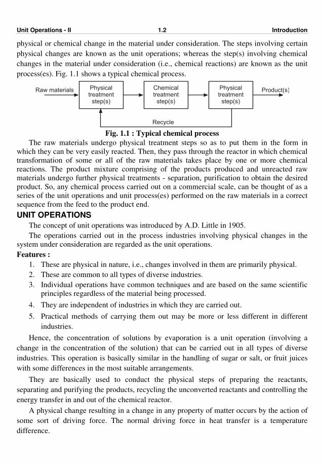
Chemical process : Every industrial chemical process is designed to produce
economically a desired product from given raw materials through a series of steps involving
Unit Operations - II 1.2 Introduction
physical or chemical change in the material under consideration. The steps involving certain
physical changes are known as the unit operations; whereas the step(s) involving chemical
changes in the material under consideration (i.e., chemical reactions) are known as the unit
process(es). Fig. 1.1 shows a typical chemical process.
Physicaltreatment
step(s)
Raw materials Chemicaltreatment
step(s)
Physicaltreatment
step(s)
Product(s)
Recycle Fig. 1.1 : Typical chemical process
The raw materials undergo physical treatment steps so as to put them in the form in
which they can be very easily reacted. Then, they pass through the reactor in which chemical
transformation of some or all of the raw materials takes place by one or more chemical
reactions. The product mixture comprising of the products produced and unreacted raw
materials undergo further physical treatments - separation, purification to obtain the desired
product. So, any chemical process carried out on a commercial scale, can be thought of as a
series of the unit operations and unit process(es) performed on the raw materials in a correct
sequence from the feed to the product end.
UNIT OPERATIONS
The concept of unit operations was introduced by A.D. Little in 1905.
The operations carried out in the process industries involving physical changes in the
system under consideration are regarded as the unit operations.
Features :
1. These are physical in nature, i.e., changes involved in them are primarily physical.
2. These are common to all types of diverse industries.
3. Individual operations have common techniques and are based on the same scientific
principles regardless of the material being processed.
4. They are independent of industries in which they are carried out.
5. Practical methods of carrying them out may be more or less different in different
industries.
Hence, the concentration of solutions by evaporation is a unit operation (involving a
change in the concentration of the solution) that can be carried out in all types of diverse
industries. This operation is basically similar in the handling of sugar or salt, or fruit juices
with some differences in the most suitable arrangements.
They are basically used to conduct the physical steps of preparing the reactants,
separating and purifying the products, recycling the unconverted reactants and controlling the
energy transfer in and out of the chemical reactor.
A physical change resulting in a change in any property of matter occurs by the action of
some sort of driving force. The normal driving force in heat transfer is a temperature
difference.
Unit Operations - II 1.3 Introduction
Broadly, unit operations are Mechanical Operations, e.g., size reduction (crushing and
grinding), filtration, size separation, etc. Fluid Flow Operations in which the pressure
difference acts as a driving force, Heat Transfer (Operations) in which the temperature
difference acts as a driving force and Mass Transfer Operations in which the concentration
difference/ gradient acts as a driving force, e.g., distillation, gas absorption, drying, etc.
The theory of unit operations is based on the fundamental laws of physical sciences such
as law of conservation of mass, law of conservation of energy, Newton's laws of motion,
Ideal gas law, Dalton's law of partial pressure, Newton's law of cooling, Raoult's law, etc.
CLASSIFICATION OF UNIT OPERATIONS
1. Fluid flow : It is concerned with the principles that determine the flow or
transportation of any fluid from one location to another.
2. Mechanical operations : These involve size reduction of solids by crushing,
grinding and pulverising, mixing, conveying and mechanical separations such as decantation,
filtration, settling and sedimentation, screening, flotation, etc.
3. Heat transfer : It deals with a study of the rate of heat energy transfer from one
place to another owing to the existence of a temperature difference. It deals with the
determination of rates of heat transfer. Heat transfer occurs in heating, cooling, phase
change, evaporation, drying, distillation, etc. The modes/mechanisms by which heat transfer
may occur are conduction, convection and radiation.
4. Mass transfer : It is concerned with the transfer of mass from one phase to another
distinct phase. Mass transfer operations depend on molecules diffusing or vaporising from
one distinct phase to another and are based on (or they utilise) differences in vapour pressure,
solubility, or diffusivity. Molecular diffusion and turbulent/eddy diffusion are the
mechanisms of mass transfer. Mass transfer operations include separation techniques like
distillation, gas absorption, drying, extraction, crystallisation, etc.
This text covers heat and mass transfer operations - a part portion of the unit operations
of chemical engineering.
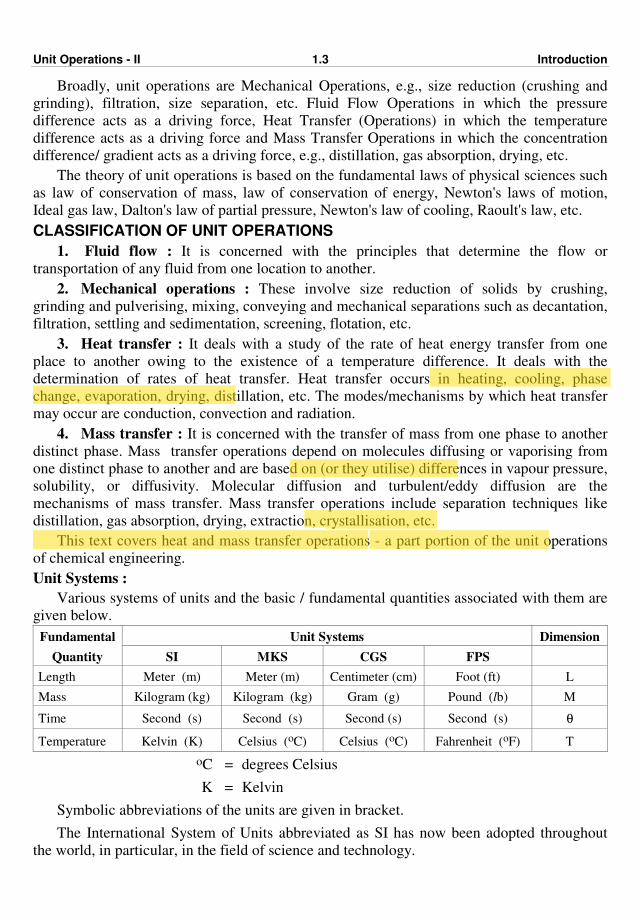
Unit Systems :
Various systems of units and the basic / fundamental quantities associated with them are
given below.
Fundamental Unit Systems Dimension
Quantity SI MKS CGS FPS
Length Meter (m) Meter (m) Centimeter (cm) Foot (ft) L
Mass Kilogram (kg) Kilogram (kg) Gram (g) Pound (lb) M
Time Second (s) Second (s) Second (s) Second (s) θ
Temperature Kelvin (K) Celsius (oC) Celsius (oC) Fahrenheit (oF) T
oC = degrees Celsius
K = Kelvin
Symbolic abbreviations of the units are given in bracket.
The International System of Units abbreviated as SI has now been adopted throughout
the world, in particular, in the field of science and technology.

Unit Operations - II 1.4 Introduction
BASIC SI UNITS
Mass : kilogram (kg)
Length : meter (m)
Time : second (s)
Temperature : kelvin (K)
Mole : kilogram mole (kmol)
Force : newton (N)
Pressure : newton / (meter)2 [N/m2 = Pa (pascal)]
Energy : newton · meter (N.m) = J (joule)
Power : newton · meter / second ((N.m)/s = J/s = W)
1. Pressure : The units of pressure in SI, MKS and FPS systems are N/m2 (known as
pascal, symbol Pa), kgf/cm2 and lbf / in2 (known as psi) respectively.
1 atm = 760 torr (or mm Hg) = 101325 N/m2 or Pa
= 101.325 kPa = 1.033 kgf/cm2
2. Work / Energy : The units of work (energy) in SI, MKS, CGS and FPS systems are
joule (J), m.kgf, erg and ft.lbf respectively.
3. Heat : The units of heat in SI, MKS, CGS and FPS systems are joule (J), kilocalorie
(kcal), calorie (cal) and British thermal unit (Btu) respectively.
1 cal = 4.187 J,
1 Btu = 1055.056 J
In the SI system, heat flow/heat flux is usually expressed in watts (W).
Some of the prefixes for SI units :
(i) giga (G) – multiply by 109
(ii) mega (M) – multiply by 106
(iii) kilo (k) – multiply by 103
(iv) milli (m) – multiply by 10–3
(v) micro (µ) – multiply by 10–6
(vi) nano (n) – multiply by10–9
Unit Operations - II 1.5 Introduction
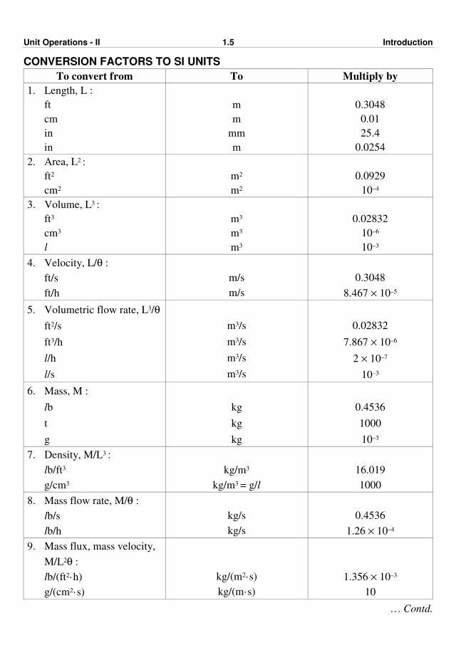
CONVERSION FACTORS TO SI UNITS
To convert from To Multiply by
1. Length, L :
ft
cm
in
in
m
m
mm
m
0.3048
0.01
25.4
0.0254
2. Area, L2 :
ft2
cm2
m2
m2
0.0929
10–4
3. Volume, L3 :
ft3
cm3
l
m3
m3
m3
0.02832
10–6
10–3
4. Velocity, L/θ :
ft/s
ft/h
m/s
m/s
0.3048
8.467 × 10⁻⁵
5. Volumetric flow rate, L3/θ
ft2/s
ft3/h
l/h
l/s
m3/s
m3/s
m3/s
m3/s
0.02832
7.867 × 10⁻⁶
2 × 10⁻⁷
10–3
6. Mass, M :
lb
t
g
kg
kg
kg
0.4536
1000
10–3
7. Density, M/L3 :
lb/ft3
g/cm3
kg/m3
kg/m3 = g/l
16.019
1000
8. Mass flow rate, M/θ :
lb/s
lb/h
kg/s
kg/s
0.4536
1.26 × 10⁻⁴
9. Mass flux, mass velocity,
M/L2θ :
lb/(ft2·h)
g/(cm2·s)
kg/(m2·s)
kg/(m·s)
1.356 × 10⁻³
10
… Contd.

Unit Operations - II 1.6 Introduction
10. Molar flux, molar mass
velocity, mole / L2θ :
lbmol / (ft2 · h)
gmol / (cm2 · s)
kmol / (m2 · s)
kmol / (m2 · s)
1.336 × 10⁻³
10
11. Force, F :
lbf
kgf
dyn
N
N
N
4.448
9.807
10–5
12. Pressure, F/L2 :
lbf/ft2
std. atm
std. atm
in Hg
in H2O
dyn/cm2
mmHg
torr
bar
kgf/cm2
N/m2 = Pa
N/m2 = Pa
kPa
N/m2 = Pa
N/m2 = Pa
N/m2 = Pa
N/m2 = Pa
N/m2 = Pa
N/m2 = Pa
N/m2 = Pa
47.88
1.0325 × 10⁵
101.325
3.386
249.1
10–1
133.3
133.3
105
9.808 × 10⁴
13. Energy, work, heat, FL :
cal
Btu
kcal
erg
kW·h
N·m = J
N·m = J
N·m = J
N·m = J
N·m = J
4.187
1055
4187
10–7
3.6 × 10⁶
14. Enthalpy, FL/M :
Btu/lb
cal/g
kcal/kg
(N.m)/kg = J/kg
(N.m)/kg = J/kg
(N.m)/kg = J/kg
2326
4187
4187
15. Molar enthalpy, FL/mole
Btu/lbmol
cal/gmol
(N.m)/mol = J/mol
(N.m)/mol = J/mol
2326
4187
… Contd.

Unit Operations - II 1.7 Introduction
16. Heat capacity, specific
heat, FL/MT :
Btu/(lb · oF)
cal/(g · oC)
N.m/(kg·K) = J/(kg·K)
N.m/(kg·K) = J/(kg·K)
4187
4187
17. Molar heat capacity,
FL/mole T :
Btu/(lbmol · oF)
cal/(gmol · oC)
N.m/(kmol·K) = J/(kmol·K)
N.m/(kmol·K) = J/(kmol·K)
4187
4187
18. Energy flux, FL/L2θ :
Btu/(ft2 · h)
cal/(cm2 · s)
N.m/(m2 · s) = W/m2
N.m/(m2 · s) = W/m2
3.155
4.187 × 10⁴
19. Thermal conductivity, FL2/L2θT = FL/L2θ (T/L) :
Btu·ft / (ft2 · h · oF)
kcal·m/(m2·h·oC)
cal·cm/(cm2 · s · oC)
N.m/(m·s·K) = W/(m·K)
N.m/(m·s·K) = W/(m·K)
N.m/(m·s·K) = W/(m·K)
1.7307
1.163
418.7
20. Heat transfer coefficient, FL/L2θT :
Btu/(ft2 · h · oF)
cal/(cm2 · s · oC)
kcal/(m2 · h · oC)
N.m/(m2 · s · K) = W/(m2·K)
N.m/(m2 · s · K) = W/(m2·K)
N.m/(m2 · s · K) = W/(m2·K)
5.679
4.187 × 10⁴
1.163
21. Power, FL/θ
(ft· lbf)/s
hp
Btu/h
kcal/h
(N.m)/s = W
(N.m)/s = W
(N.m)/s = W
(N.m)/s = W
1.356
745.7
0.2931
1.163
22. Viscosity, M/Lθ
P (poise ≡ g/(cm.s)
cP
lb/(ft.s)
kg/(m.s) = (N.s)/m2
kg/(m.s) = (N.s)/m2
= Pa·s
kg/(m.s)
0.10
0.001
1.488

Unit Operations - II 1.8 Introduction
While writing the units of fundamental or derived quantity, please remember the
following :
1. Correct : 10 kgf.m incorrect : 10 kgfm
2. Correct : 10 kg incorrect : 10 kgs … no plural form of the unit symbol.
3. Correct : 10 cm incorrect : 10 cm.
… no period (full stop) at the end of the unit symbol.
4. Correct : 10000 W/(m2.K) incorrect : 10000 W/m2·K
5. Correct : 10 kW incorrect : 10 k W
Temperature intervals or differences are related by :
1 deg C = 1.8 deg F = 1 K
20 deg C = 20 K
ppp

(2.1)
CHAPTER TWO
CONDUCTION
Heat transfer deals with the study of rates at which exchange of heat takes place between
a hot source and a cold receiver. In process industries there are many operations which
involve transfer of energy in the form of heat, e.g., evaporation, distillation, drying, etc. and
also chemical reactions carried on a commercial scale take place with evolution or
absorption of heat. It is also necessary to prevent the loss of heat from a hot vessel or a pipe
system to the ambient air. In all these cases, the major problem is that of transfer of heat at
the desired rate. The knowledge of laws of heat transfer, mechanisms of heat transfer and
process heat transfer equipments is of great importance from a stand point of controlling the
flow of heat in the desired manner.
It is well established fact that if two bodies at different temperatures are brought into
thermal contact, heat flows from a hot body to a relatively cold body (second law of
thermodynamics). The net flow of heat is always in the direction of decrease in the
temperature. Thus, heat is defined as a form of energy which is in transit between a hot
source and a cold receiver. The transfer of heat solely depends upon the temperatures of the
two bodies/substances/parts of a system. In other words, temperature can be termed as the
level of thermal (heat) energy, i.e., high temperature of a body is the indication of high level
of heat energy content of the body.
Heat may flow by any one or more of the three basic mechanisms, namely, conduction,
convection, and radiation. We will first see these three modes of heat transfer in brief and
then we will consider heat conduction through solids in detail.
Conduction : It is the transfer of heat from one part of a body to the another part of the
same body or from one body to another which is in physical contact with it, without
appreciable displacement of particles of a body. Conduction is restricted to the flow of heat
in solids. Examples of conduction : Heat flow through the brick wall of a furnace, the metal
sheet of a boiler and the metal wall of a heat exchanger tube.
Convection : It is the transfer of heat from one point to another point within a fluid
(gas or liquid) by mixing of hot and cold portions of the fluid. It is attributed to the
macroscopic motion of fluid. Convection is restricted to the flow of heat in fluids and is
closely associated with fluid mechanics. In natural convection, the fluid motion results from
the difference in densities of the warmer and cooler fluid arising from the temperature
difference in the fluid mass. In forced convection, the fluid motion is produced by
mechanical means such as an agitator, a fan or pump. Examples of heat transfer mainly by
convection are : heating of room by means of a steam radiator, heating of water in cooking
pans, heat flow to a fluid pumped through a heated pipe.
Unit Operations – II 2.2 Conduction
Radiation : Radiation refers to the transfer of heat energy from one body to another
through space, not in contact with it, by electromagnetic waves. Examples of heat transfer by
radiation mode are : the transfer of heat from the sun to the earth and the loss of heat from an
unlagged steam pipe to the ambient air.
Conduction as well as convection occurs only in the presence of material medium
whereas radiation can occur even in vacuum and no material medium is required for heat
flow by radiation. It is observed that heat flow by conduction is slow, faster by convection
and the fastest by radiation mode.
CONDUCTION :
It is our common observation that when some material object is heated at one of its
locations, then in a short while its remaining parts also get heated. This shows that heat flows
through the material object from a high temperature region to a low temperature region. The
flow of heat in this manner is called as heat conduction or simply conduction, wherein the
particles of object participate in the process but they do not move bodily from the hot or high
temperature region to the cold or low temperature region.
Conduction is the mode of heat transfer in which a material medium transporting the heat
remains at rest. The heat conduction occurs by the migration of molecules and more
effectively by the collision of the molecules vibrating around relatively fixed positions. In
liquids and solids where little or no migration occurs, heat is transferred by the collision of
vibrating molecules. [The molecules of a substance are always in a state of vibration. When
the substance is heated at one of its locations, the molecules of that location receive energy
and they begin to vibrate with larger amplitudes and as a result of increase in their amplitude,
they will collide with the neighbouring molecules and in the process they transfer a part of
their energy to the neighbouring molecules. This process occurs repeatedly and thus results
in heat flow from one molecule to another along the heat flow path i.e. through the
substance.]
Conduction refers to the mode of heat transfer in which the heat flow through the
material medium occurs without actual migration of particles of the medium from a region of
higher temperature to a region of lower temperature.
It is a fact that conduction occurs in solids, liquids and gases but pure conduction is
found to present only in solids, with gases and liquids it is present with convection, so we
will consider here heat conduction in solids for better understanding of conduction
mechanism as convection is not present in solids.
In this chapter, we restrict our discussion to steady state unidirectional heat
conduction in solids.
By steady state heat flow we mean that the situation of heat flow in which the
temperature at any location along the heat flow path does not vary with time and the rate of
heat transfer does not vary with time. In other words, it is the heat flow under conditions of
constant temperature distribution-temperature is a function of location only, i.e., temperature
varies with location but not with time. Hence, steady state heat conduction is the heat transfer
by conduction under conditions of constant temperature distribution.

Unit Operations – II 2.3 Conduction
By unidirectional or one dimensional heat flow we mean that the flow of heat occurring
only in one direction, i.e., along one of the axes of the respective coordinate system used.
(For example, say along the x-direction in case of a Cartesian co-ordinate system).
Fourier's Law :
The physical law governing the transfer of heat through a uniform material (whenever a
temperature difference exists) by a conduction mode was given by the French scientist :
Joseph Fourier.
Fourier's law states that the rate of heat flow by conduction through a uniform (fixed)
material is directly proportional to the area normal to the direction of the heat flow and the
temperature gradient in the direction of the heat flow.
Mathematically, the Fourier's law of heat conduction for steady state heat flow is given
by
Q ∝ A [– dT/dn] … (2.1)
Q = – kA [dT/dn] … (2.2)
where Q is the rate of heat flow/transfer in watts (W), A is the area normal to the direction of
heat flow in m2, T is the temperature in K, n is the distance measured normal to the surface,
i.e., the length of conduction path along the heat flow in m, dT/dn is the rate of change of
temperature with distance measured in the direction of heat flow (called as temperature
gradient) in K/m. k is a constant of proportionality and is called the thermal conductivity. It
is the characteristic property of a material through which heat flows.
The negative sign is incorporated in equation (2.2) because the temperature gradient is
negative (since with an increase in n there is a decrease in T, i.e., temperature decreases in
the direction of heat flow) and it makes the heat flow positive in the direction of temperature
decrease.
The Fourier's law for a steady state unidirectional (say in the x-direction) heat conduction
then becomes
Q = – kA [dT/dx] … (2.3)
q = Q/A = – k [dT/dx] … (2.4)
where Q is the rate of heat flow, i.e., heat flow per unit time in W, and q is the heat flux,
i.e., the rate of heat flow per unit area in W/m2 (in the x-direction). In further discussion
we will make use of Equation (2.3). The Fourier's law [equation (2.3)] is a fundamental
differential equation of heat transfer by conduction. It is simply a definition of k.
[The heat flux is defined as the amount of heat transfer per unit area per unit time or the
rate of heat transfer per unit area, Q/A.]
One Dimensional Steady State conduction :
Steady state heat conduction is a simpler case in the sense that the temperature does not
vary with time. T is independent of time and is a function of position in the conducting solid.
Unit Operations – II 2.4 Conduction
One dimensional heat conduction implies that the temperature gradient exists only in one
direction which makes the heat flow unidirectional. The cases of heat flow through a slab
(plane wall), a circular cylinder, a sphere and long fins can be analysed by a one dimensional
steady state conduction. In the discussion to follow we will treat heat flow to be in
x-direction only.
In discussion to follow we assume that k does not vary with temperature.
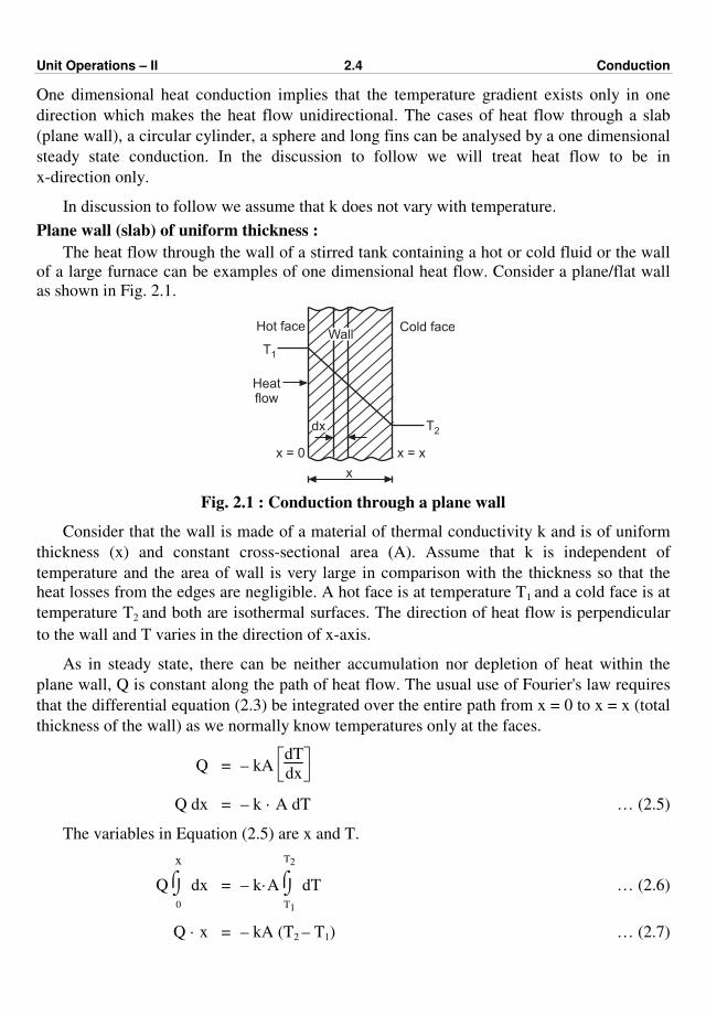
Plane wall (slab) of uniform thickness :
The heat flow through the wall of a stirred tank containing a hot or cold fluid or the wall
of a large furnace can be examples of one dimensional heat flow. Consider a plane/flat wall
as shown in Fig. 2.1.
Heatflow
T1
Hot faceWall
Cold face
T2dx
x = xx = 0
x
Fig. 2.1 : Conduction through a plane wall
Consider that the wall is made of a material of thermal conductivity k and is of uniform
thickness (x) and constant cross-sectional area (A). Assume that k is independent of
temperature and the area of wall is very large in comparison with the thickness so that the
heat losses from the edges are negligible. A hot face is at temperature T1 and a cold face is at
temperature T2 and both are isothermal surfaces. The direction of heat flow is perpendicular
to the wall and T varies in the direction of x-axis.
As in steady state, there can be neither accumulation nor depletion of heat within the
plane wall, Q is constant along the path of heat flow. The usual use of Fourier's law requires
that the differential equation (2.3) be integrated over the entire path from x = 0 to x = x (total
thickness of the wall) as we normally know temperatures only at the faces.
Q = – kA
dT
dx
Q dx = – k · A dT … (2.5)
The variables in Equation (2.5) are x and T.
Q ⌡⌠0
x
dx = – k·A ⌡⌠T1
T2
dT … (2.6)
Q · x = – kA (T2 – T1) … (2.7)
Unit Operations – II 2.5 Conduction
Rearranging, we get
Q = kA (T1 – T2)
x … (2.8)
Q = k·A
x · ∆T … (2.9)
where ∆T = (T1 – T2)
Q = ∆T
x/kA =
∆T
R … (2.10)
where R (= x/kA) is the thermal resistance (of the wall material of thickness x), Q is the rate
of heat flow (rate of heat transfer) and ∆T is the driving force for heat flow.
Equation (2.10) equates the rate of heat flow to the ratio of driving force to thermal
resistance.
The reciprocal of resistance is called the conductance, which for heat conduction is :
Conductance = 1/R = 1/(x/kA) = k.A/x … (2.11)
Both the resistance and conductance depend upon the dimensions of a solid as well as on
the thermal conductivity, a property of the material.
When k varies linearly with T (Equation 2.12), Equation (2.10) can be used rigorously by
taking an average value –k for k.
–k may be obtained either by using the arithmetic average of
the individual values of k at surface temperatures T1 and T2 [–k = (k1 + k2)/2] or by calculating
the arithmetic average of temperatures [(T1 + T2)/2] and using the value of k at that
temperature. One can take linear variation of k with T under integration sign and integrate
the equation.
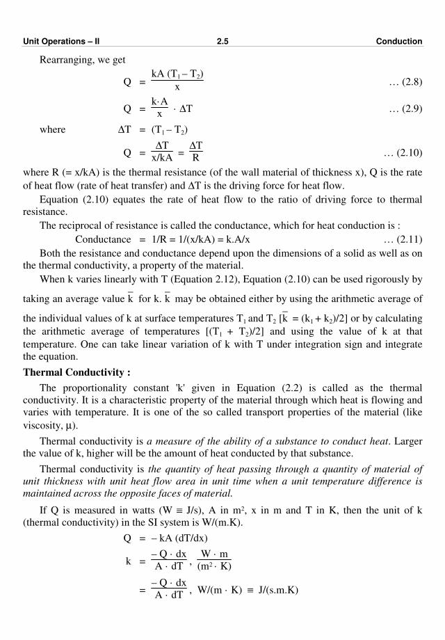
Thermal Conductivity :
The proportionality constant 'k' given in Equation (2.2) is called as the thermal
conductivity. It is a characteristic property of the material through which heat is flowing and
varies with temperature. It is one of the so called transport properties of the material (like
viscosity, µ).
Thermal conductivity is a measure of the ability of a substance to conduct heat. Larger
the value of k, higher will be the amount of heat conducted by that substance.
Thermal conductivity is the quantity of heat passing through a quantity of material of
unit thickness with unit heat flow area in unit time when a unit temperature difference is
maintained across the opposite faces of material.
If Q is measured in watts (W ≡ J/s), A in m2, x in m and T in K, then the unit of k
(thermal conductivity) in the SI system is W/(m.K).
Q = – kA (dT/dx)
k = – Q · dx
A · dT ,
W · m
(m2 · K)
= – Q · dx
A · dT , W/(m · K) ≡ J/(s.m.K)
Unit Operations – II 2.6 Conduction
Thermal conductivity depends upon the nature of material and its temperature. Thermal
conductivities of solids are higher than that of liquids and liquids are having higher thermal
conductivities than for gases.
In general, thermal conductivity of gases ranges from 0.006 to 0.6 W/(m·K) while that of
liquids ranges from 0.09 to 0.7 W/(m·K). Thermal conductivity of metals varies from
2.3 to 420 W/(m·K). The materials having higher values of thermal conductivity are referred
to as good conductors of heat, e.g., metals. The best conductor of heat is silver
[k = 420 W/(m·K)] followed by red copper [k = 395 W/(m·K)], gold [k = 302 W/(m·K)] and
aluminium [k = 210 W/(m·K)]. The materials having low values of thermal conductivity
[less than 0.20 W/(m·K)] are called as and used as heat insulators to minimise the rate of
heat flow. e.g. asbestos, glass wool, cork, etc.
For small temperature ranges, thermal conductivity may be taken as constant but for
large temperature ranges, it varies linearly with temperature and the variation of the thermal
conductivity with temperature is given by the relationship
k = a + bT … (2.12)
where a and b are empirical constants and T is the temperature in K.
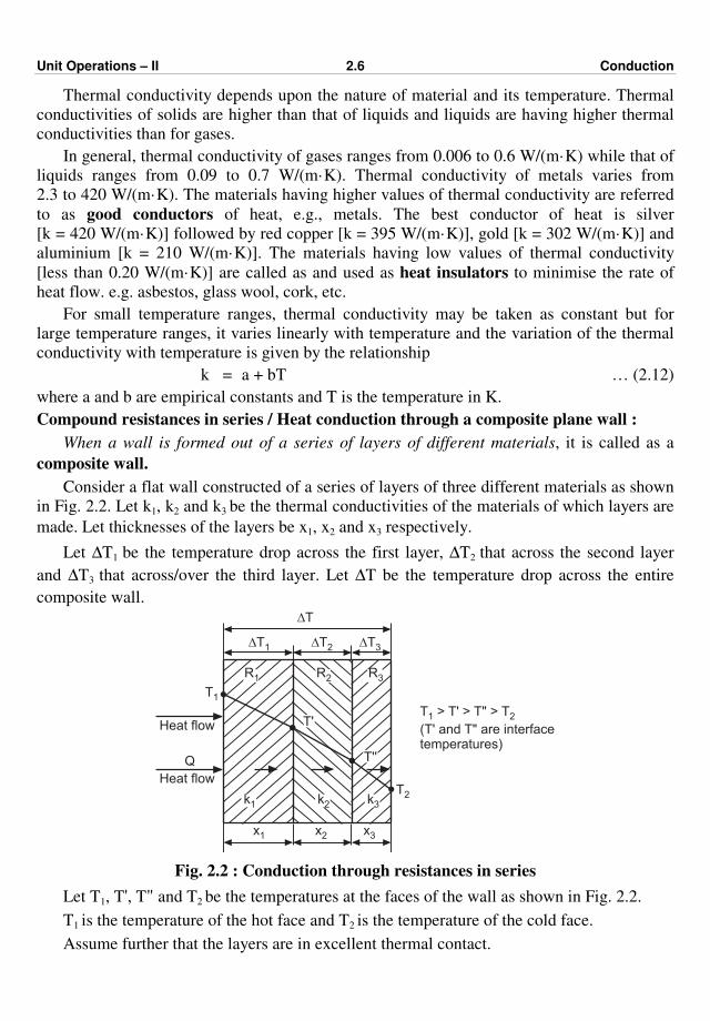
Compound resistances in series / Heat conduction through a composite plane wall :
When a wall is formed out of a series of layers of different materials, it is called as a
composite wall.
Consider a flat wall constructed of a series of layers of three different materials as shown
in Fig. 2.2. Let k1, k2 and k3 be the thermal conductivities of the materials of which layers are
made. Let thicknesses of the layers be x1, x2 and x3 respectively.
Let ∆T1 be the temperature drop across the first layer, ∆T2 that across the second layer
and ∆T3 that across/over the third layer. Let ∆T be the temperature drop across the entire
composite wall.
DT
DT1 DT2 DT3
R1 R2 R3
T'
T''
T1
Heat flow
Heat flow
Q
k1 k2 k3
T2
x1 x2 x3
T > T' > T" > T
(T' and T" are interfacetemperatures)
1 2
Fig. 2.2 : Conduction through resistances in series
Let T1, T', T" and T2 be the temperatures at the faces of the wall as shown in Fig. 2.2.
T1 is the temperature of the hot face and T2 is the temperature of the cold face.
Assume further that the layers are in excellent thermal contact.
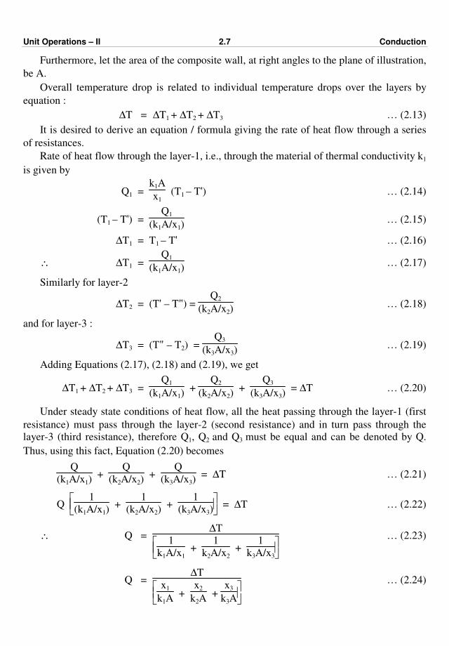
Unit Operations – II 2.7 Conduction
Furthermore, let the area of the composite wall, at right angles to the plane of illustration,
be A.
Overall temperature drop is related to individual temperature drops over the layers by
equation :
∆T = ∆T1 + ∆T2 + ∆T3 … (2.13)
It is desired to derive an equation / formula giving the rate of heat flow through a series
of resistances.
Rate of heat flow through the layer-1, i.e., through the material of thermal conductivity k1
is given by
Q1 = k1A
x1 (T1 – T') … (2.14)
(T1 – T') = Q1
(k1A/x1) … (2.15)
∆T1 = T1 – T' … (2.16)
∴ ∆T1 = Q1
(k1A/x1) … (2.17)
Similarly for layer-2
∆T2 = (T' – T") = Q2
(k2A/x2) … (2.18)
and for layer-3 :
∆T3 = (T" – T2) = Q3
(k3A/x3) … (2.19)
Adding Equations (2.17), (2.18) and (2.19), we get
∆T1 + ∆T2 + ∆T3 = Q1
(k1A/x1) +
Q2
(k2A/x2) +
Q3
(k3A/x3) = ∆T … (2.20)
Under steady state conditions of heat flow, all the heat passing through the layer-1 (first
resistance) must pass through the layer-2 (second resistance) and in turn pass through the
layer-3 (third resistance), therefore Q1, Q2 and Q3 must be equal and can be denoted by Q.
Thus, using this fact, Equation (2.20) becomes
Q
(k1A/x1) +
Q
(k2A/x2) +
Q
(k3A/x3) = ∆T … (2.21)
Q
1
(k1A/x1) +
1
(k2A/x2) +
1
(k3A/x3) = ∆T … (2.22)
∴ Q = ∆T
1
k1A/x1 +
1
k2A/x2 +
1
k3A/x3
… (2.23)
Q = ∆T
x1
k1A +
x2
k2A +
x3
k3A
… (2.24)

Unit Operations – II 2.8 Conduction
Let R1, R2 and R3 be the thermal resistances offered by the layer-1, 2 and 3 respectively.
R1, R2 and R3 are given as :
R1 = x1/k1A … (2.25)
R2 = x2/k2A … (2.26)
and R3 = x3/k3A … (2.27)
With this Equation (2.24) becomes
Q = ∆T
R1 + R2 + R3 … (2.28)
If R is the overall resistance, then for resistances in series, we have :
R = R1 + R2 + R3 … (2.29)
Equation (2.28) becomes :
Q = ∆T
R … (2.30)
Equation (2.30) is used to calculate the rate of heat flow/heat transfer. It is the ratio of the
overall temperature drop (driving force) to the overall resistance of the composite wall.
Equation (2.30) is the same as the equation for the rate of any process :
Rate of transfer process = Driving force
Resistance
One can calculate the temperatures at the interfaces of layers of which the wall is made
by making use of the following relation :
∆T
R =
∆T1
R1 =
∆T2
R2 =
∆T3
R3 … (2.31)
Based upon the thickness and thermal conductivity of a layer, temperature drop in that
layer may be large or small fraction of the total temperature drop. A thin layer with a low
thermal conductivity value may cause a much larger temperature drop and a steeper thermal
gradient than a thick layer having a high thermal conductivity.
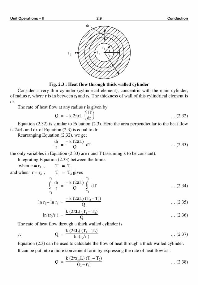
Heat flow through a cylinder :
Consider a thick walled hollow cylinder as shown in Fig. 2.3 of inside radius r1, outside
radius r2 and length L. Let k be the thermal conductivity of the material of cylinder.
Let the temperature of the inside surface be T1 and that of the outside surface be T2.
Assume that T1 > T2, therefore heat flows from the inside of the cylinder to the outside. It is
desired to calculate the rate of heat flow for this case.
Unit Operations – II 2.9 Conduction
r1
T1 r2
rT2
dr
Fig. 2.3 : Heat flow through thick walled cylinder
Consider a very thin cylinder (cylindrical element), concentric with the main cylinder,
of radius r, where r is in between r1 and r2. The thickness of wall of this cylindrical element is
dr.
The rate of heat flow at any radius r is given by
Q = – k 2πrL
dT
dr … (2.32)
Equation (2.32) is similar to Equation (2.3). Here the area perpendicular to the heat flow
is 2πrL and dx of Equation (2.3) is equal to dr.
Rearranging Equation (2.32), we get
dr
r =
– k (2πL)
Q dT … (2.33)
the only variables in Equation (2.33) are r and T (assuming k to be constant).
Integrating Equation (2.33) between the limits
when r = r1 , T = T1
and when r = r2 , T = T2 gives
⌡⌠
r1
r2
dr
r =
– k (2πL)
Q ⌡⌠
T1
T2
dT … (2.34)
ln r2 – ln r1 = – k (2πL) (T2 – T1)
Q … (2.35)
ln (r2/r1) = k (2πL) (T1 – T2)
Q … (2.36)
The rate of heat flow through a thick walled cylinder is
∴ Q = k (2πL) (T1 – T2)
ln (r2/r1) … (2.37)
Equation (2.3) can be used to calculate the flow of heat through a thick walled cylinder.
It can be put into a more convenient form by expressing the rate of heat flow as :
Q = k (2πrmL) (T1 – T2)
(r2 – r1) … (2.38)
Unit Operations – II 2.10 Conduction
where rm is the logarithmic mean radius and is given by
rm = (r2 – r1)
ln (r2/r1) =
(r2 – r1)
2.303 log (r2/r1) … (2.39)
Am = 2πrmL … (2.40)
Am is called the logarithmic mean area.
Equation (2.38) becomes :
Q = k Am (T1 – T2)
(r2 – r1) … (2.41)
Q = (T1 – T2)
(r2 – r1) / k Am =
∆T
R
where R = (r2 – r1) / kAm
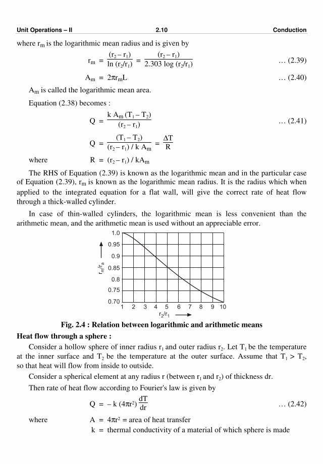
The RHS of Equation (2.39) is known as the logarithmic mean and in the particular case
of Equation (2.39), rm is known as the logarithmic mean radius. It is the radius which when
applied to the integrated equation for a flat wall, will give the correct rate of heat flow
through a thick-walled cylinder.
In case of thin-walled cylinders, the logarithmic mean is less convenient than the
arithmetic mean, and the arithmetic mean is used without an appreciable error.
r/r
am
r /r12
1 2 3 4 5 6 7 8 9 10
1.0
0.95
0.9
0.85
0.8
0.75
0.70
Fig. 2.4 : Relation between logarithmic and arithmetic means
Heat flow through a sphere :
Consider a hollow sphere of inner radius r1 and outer radius r2. Let T1 be the temperature
at the inner surface and T2 be the temperature at the outer surface. Assume that T1 > T2,
so that heat will flow from inside to outside.
Consider a spherical element at any radius r (between r1 and r2) of thickness dr.
Then rate of heat flow according to Fourier's law is given by
Q = – k (4πr2) dT
dr … (2.42)
where A = 4πr2 = area of heat transfer
k = thermal conductivity of a material of which sphere is made
Unit Operations – II 2.11 Conduction
Rearranging Equation (2.42), we get
dr
r2 = – 4πk
Q dT … (2.43)
Integrating Equation (2.43) between the limits :
when r = r1 , T = T1
and r = r2 , T = T2
⌡⌠
r1
r2
dr
r2 = – 4πk
Q ⌡⌠
T1
T2
dT … (2.44)
– 1
r
r2
r1
= – 4πk
Q (T1 – T2) … (2.45)
1
r1 –
1
r2 =
4πk
Q (T1 – T2) … (2.46)
Rearranging, we get
Q = 4πk (T1 – T2)
1
r1 –
1
r2
… (2.47)
Q = 4π r1 r2 k (T1 – T2)
(r2 – r1) … (2.48)
rm = r1 r2 = mean radius which is geometric mean for sphere.
∴ Equation (2.48) becomes :
Q = 4π r
2
m k (T1 – T2)
(r2 – r1) … (2.49)
Thermal Insulation :
Process equipments such as a reaction vessel, reboiler, distillation column, evaporator,
etc. or a steam pipe will lose heat to the atmosphere by conduction, convection and radiation.
In such cases, the conservation of heat that is usually of steam and coal is an economic
necessity and therefore some form of lagging should be applied to the hot surfaces. In
furnaces, the surface temperature is reduced substantially by making use of a series of
insulating bricks that are poor conductors of heat.
Insulation is necessary (i) to prevent an excessive flow of heat to the surroundings from
process units and pipelines in which heat is generated, stored or conveyed at temperatures
above the surrounding temperature, (ii) to prevent an excessive flow of heat from the outside
to materials which must be kept at temperatures below that of the surroundings, (iii) to
Unit Operations – II 2.12 Conduction
provide for protection of personnel from skin damage through contact with very hot and very
cold surfaces (to provide a safe work environment) and (iv) to provide
comfortable/acceptable working environment. The working environment in the viscinity of
process units and pipelines carrying hot or cold streams can become uncomfortable and
unacceptable, if insulation is not provided. In a chemical plant, steam is transported to
process equipments, as per requirement, through steam lines. If the steam lines are not
insulated, then the loss of heat from these lines to the ambient air may result in the
condensation of steam, thus lowering the quality of steam and creating operational problems
in the equipments in which the steam is admitted.
The important requirements of an insulating material are as follows :
(i) It should have a low thermal conductivity.
(ii) It should withstand working temperature range.
(iii) It should have a sufficient durability and an adequate mechanical strength. This
includes resistance to moisture and the chemical environment.
(iv) It should be easy to apply, non-toxic, readily available, inexpensive (low basic
material cost, installation cost and maintenance cost).
(v) It should not create a fire hazard.
Cork [k = 0.025 W/(m·K)], asbestos (k = 0.10), glass wool (k = 0.024), 85 percent
magnesia (k = 0.04) are commonly employed lagging materials in industry. Cork is common
in refrigeration plants. 85% magnesia with asbestos, glass wool are widely used for lagging
steam pipes. Thin aluminium sheeting is often used to protect the lagging.
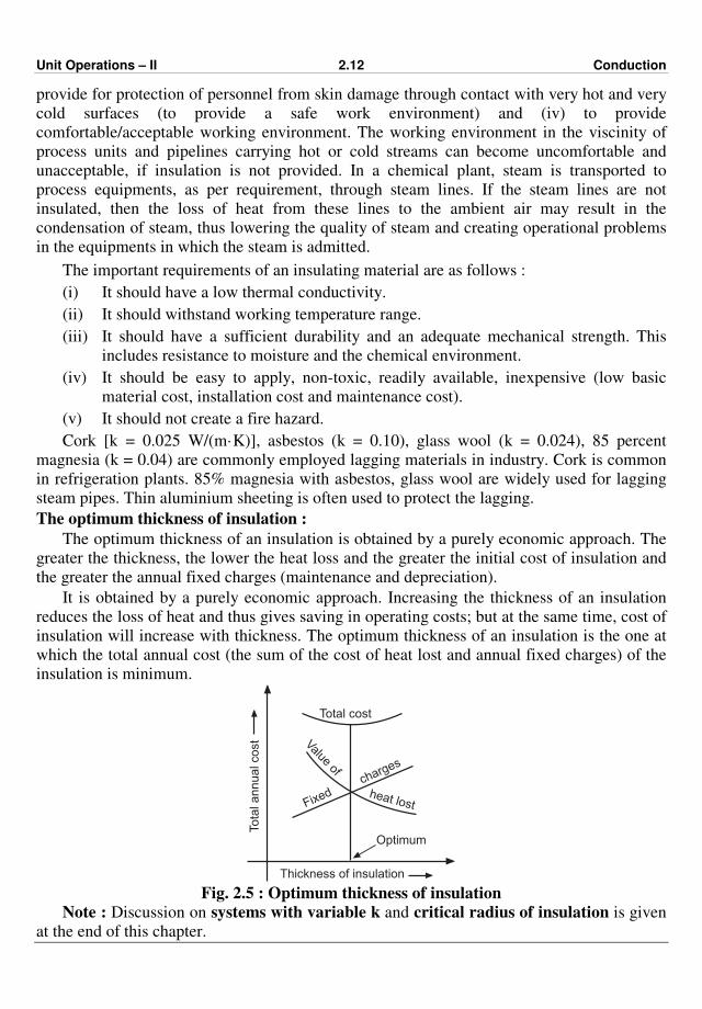
The optimum thickness of insulation :
The optimum thickness of an insulation is obtained by a purely economic approach. The
greater the thickness, the lower the heat loss and the greater the initial cost of insulation and
the greater the annual fixed charges (maintenance and depreciation).
It is obtained by a purely economic approach. Increasing the thickness of an insulation
reduces the loss of heat and thus gives saving in operating costs; but at the same time, cost of
insulation will increase with thickness. The optimum thickness of an insulation is the one at
which the total annual cost (the sum of the cost of heat lost and annual fixed charges) of the
insulation is minimum.
Optimum
Total cost
Fixedcharges
heat lost
Valueof
Tota
l annual cost
Thickness of insulation Fig. 2.5 : Optimum thickness of insulation
Note : Discussion on systems with variable k and critical radius of insulation is given
at the end of this chapter.
Unit Operations – II 2.13 Conduction
SOLVED EXAMPLES
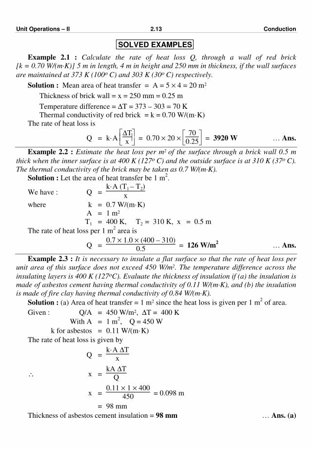
Example 2.1 : Calculate the rate of heat loss Q, through a wall of red brick
[k = 0.70 W/(m·K)] 5 m in length, 4 m in height and 250 mm in thickness, if the wall surfaces
are maintained at 373 K (100o C) and 303 K (30o C) respectively.
Solution : Mean area of heat transfer = A = 5 × 4 = 20 m2
Thickness of brick wall = x = 250 mm = 0.25 m
Temperature difference = ∆T = 373 – 303 = 70 K
Thermal conductivity of red brick = k = 0.70 W/(m·K)
The rate of heat loss is
Q = k·A
∆T
x = 0.70 × 20 ×
70
0.25 = 3920 W … Ans.
Example 2.2 : Estimate the heat loss per m2 of the surface through a brick wall 0.5 m
thick when the inner surface is at 400 K (127o C) and the outside surface is at 310 K (37o C).
The thermal conductivity of the brick may be taken as 0.7 W/(m·K).
Solution : Let the area of heat transfer be 1 m2.
We have : Q = k·A (T1 – T2)
x
where k = 0.7 W/(m·K)
A = 1 m2
T1 = 400 K, T2 = 310 K, x = 0.5 m
The rate of heat loss per 1 m2 area is
Q = 0.7 × 1.0 × (400 – 310)
0.5 = 126 W/m
2 … Ans.
Example 2.3 : It is necessary to insulate a flat surface so that the rate of heat loss per
unit area of this surface does not exceed 450 W/m2. The temperature difference across the
insulating layers is 400 K (127oC). Evaluate the thickness of insulation if (a) the insulation is
made of asbestos cement having thermal conductivity of 0.11 W/(m·K), and (b) the insulation
is made of fire clay having thermal conductivity of 0.84 W/(m·K).
Solution : (a) Area of heat transfer = 1 m2 since the heat loss is given per 1 m2 of area.
Given : Q/A = 450 W/m2, ∆T = 400 K
With A = 1 m2, Q = 450 W
k for asbestos = 0.11 W/(m·K)
The rate of heat loss is given by
Q = k·A ∆T
x
∴ x = kA ∆T
Q
x = 0.11 × 1 × 400
450 = 0.098 m
= 98 mm
Thickness of asbestos cement insulation = 98 mm … Ans. (a)
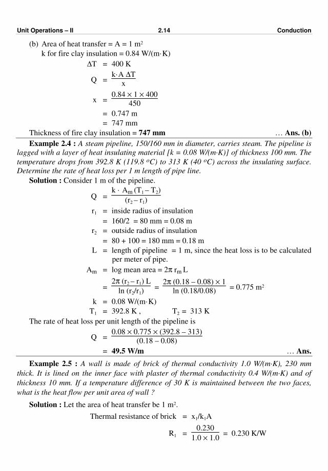
Unit Operations – II 2.14 Conduction
(b) Area of heat transfer = A = 1 m2
k for fire clay insulation = 0.84 W/(m·K)
∆T = 400 K
Q = k·A ∆T
x
x = 0.84 × 1 × 400
450
= 0.747 m
= 747 mm
Thickness of fire clay insulation = 747 mm … Ans. (b)
Example 2.4 : A steam pipeline, 150/160 mm in diameter, carries steam. The pipeline is
lagged with a layer of heat insulating material [k = 0.08 W/(m·K)] of thickness 100 mm. The
temperature drops from 392.8 K (119.8 oC) to 313 K (40 oC) across the insulating surface.
Determine the rate of heat loss per 1 m length of pipe line.
Solution : Consider 1 m of the pipeline.
Q = k · Am (T1 – T2)
(r2 – r1)
r1 = inside radius of insulation
= 160/2 = 80 mm = 0.08 m
r2 = outside radius of insulation
= 80 + 100 = 180 mm = 0.18 m
L = length of pipeline = 1 m, since the heat loss is to be calculated
per meter of pipe.
Am = log mean area = 2π rm L
= 2π (r2 – r1) L
ln (r2/r1) =
2π (0.18 – 0.08) × 1
ln (0.18/0.08) = 0.775 m2
k = 0.08 W/(m·K)
T1 = 392.8 K , T2 = 313 K
The rate of heat loss per unit length of the pipeline is
Q = 0.08 × 0.775 × (392.8 – 313)
(0.18 – 0.08)
= 49.5 W/m … Ans.
Example 2.5 : A wall is made of brick of thermal conductivity 1.0 W/(m·K), 230 mm
thick. It is lined on the inner face with plaster of thermal conductivity 0.4 W/(m·K) and of
thickness 10 mm. If a temperature difference of 30 K is maintained between the two faces,
what is the heat flow per unit area of wall ?
Solution : Let the area of heat transfer be 1 m2.
Thermal resistance of brick = x1/k1A
R1 = 0.230
1.0 × 1.0 = 0.230 K/W
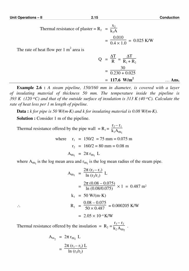
Unit Operations – II 2.15 Conduction
Thermal resistance of plaster = R2 = x2
k2A
= 0.010
0.4 × 1.0 = 0.025 K/W
The rate of heat flow per 1 m2 area is
Q = ∆T
R =
∆T
R1 + R2
= 30
0.230 + 0.025
= 117.6 W/m2 … Ans.
Example 2.6 : A steam pipeline, 150/160 mm in diameter, is covered with a layer
of insulating material of thickness 50 mm. The temperature inside the pipeline is
393 K (120 oC) and that of the outside surface of insulation is 313 K (40 oC). Calculate the
rate of heat loss per 1 m length of pipeline.
Data : k for pipe is 50 W/(m·K) and k for insulating material is 0.08 W/(m·K).
Solution : Consider 1 m of the pipeline.
Thermal resistance offered by the pipe wall = R1 = r2 – r1
k1Am1
where r1 = 150/2 = 75 mm = 0.075 m
r2 = 160/2 = 80 mm = 0.08 m
Am1 = 2π rm1
L
where Am1 is the log mean area and rm1
is the log mean radius of the steam pipe.
Am1 =
2π (r2 – r1)
ln (r2/r1) L
= 2π (0.08 – 0.075)
ln (0.08/0.075) × 1 = 0.487 m2
k1 = 50 W/(m·K)
∴ R1 = 0.08 – 0.075
50 × 0.487 = 0.000205 K/W
= 2.05 × 10⁻⁴ K/W
Thermal resistance offered by the insulation = R2 = r3 – r2
k2 Am2
.
Am2 = 2π rm2
L
= 2π (r3 – r2) L
ln (r3/r2)

Unit Operations – II 2.16 Conduction
where r3 = r2 + 50 mm
= 80 + 50 = 130 mm = 0.13 m
Am2 =
2π (0.13 – 0.08)
ln (0.13/0.08) × 1
Am2 = 0.647 m2
k2 = 0.08 W/(m·K)
∴ R2 = (0.13 – 0.08)
0.08 × 0.647 = 0.966 K/W
Total thermal resistance = R = R1 + R2
= 2.05 × 10⁻⁴ + 0.966 = 0.9662 K/W
The rate of heat loss per 1 m of the pipeline is
Q = ∆T
R =
393 – 313
0.9662
= 82.8 W/m … Ans.
Example 2.7 : A furnace is constructed with 225 mm thick of fire brick, 120 mm
of insulating brick and 225 mm of the building brick. The inside temperature is
1200 K (927 oC) and the outside temperature is 330 K (57 oC). Find the heat loss per unit
area and the temperature at the junction of the fire brick and insulating brick.
Data : k for fire brick = 1.4 W/(m·K)
k for insulating brick = 0.2 W/(m·K)
k for building brick = 0.7 W/(m·K)
Solution : Let the area of heat transfer be 1 m2. Therefore, A = 1 m
2.
F.B.
225 mm 225 mm
B.B.
T = 1200 K1 x1
x2
x3T = 330 K2
k = 1.41
120 mm
k = 0.22 k = 0.73
I.B.
Fig. Ex. 2.7
Let T1 and T2 be the temperatures at the fire brick / insulating brick and the insulating
brick/building brick junctions respectively.
Thermal resistance of the fire brick = x1
k1A
R1 = 0.225
1.4 × 1 = 0.1607 K/W

Unit Operations – II 2.17 Conduction
Thermal resistance of the insulating brick = x2
k2A
R2 = 0.120
0.2 × 1 = 0.60 K/W
Thermal resistance of the building brick = x3
k3A
R3 = 0.225
0.7 × 1 = 0.322 K/W
The heat loss per unit area is
Q = ∆T
R
where R = R1 + R2 + R3 and ∆T = T1 – T2
Q = 1200 – 330
0.1607 + 0.60 + 0.322
= 803.5 W/m2 … Ans.
Let us calculate the temperature at the junction between fire brick and insulating brick.
For steady state heat transfer, Q1 = Q. Therefore,
∆T1
R1 =
∆T
R
∆T1
∆T =
R1
R
1200 – T1
1200 – 330 =
0.1607
0.1607 + 0.60 + 0.322
T1 = 1071 K (798 oC) … Ans.
Similarly, for the junction between insulating brick and building brick, we can write :
∆T2/R2 = ∆T/R
∴ (1071 – T2)
1200 – 330 =
0.60
0.1607 + 0.6 + 0.322
T2 = 589 K (316 oC) … Ans.
Example 2.8 : A 50 mm diameter pipe of circular cross-section and with walls 3 mm
thick is covered with two concentric layers of lagging, the inner layer having a thickness of
25 mm and a thermal conductivity of 0.08 W/(m·K), and the outer layer having a thickness of
40 mm and a thermal conductivity of 0.04 W/(m·K). Estimate the rate of heat loss per metre
length of pipe if the temperature inside the pipe is 550 K (277 oC) and the outside surface
temperature is 330 K (57 oC). k for pipe is 45 W/(m·K).
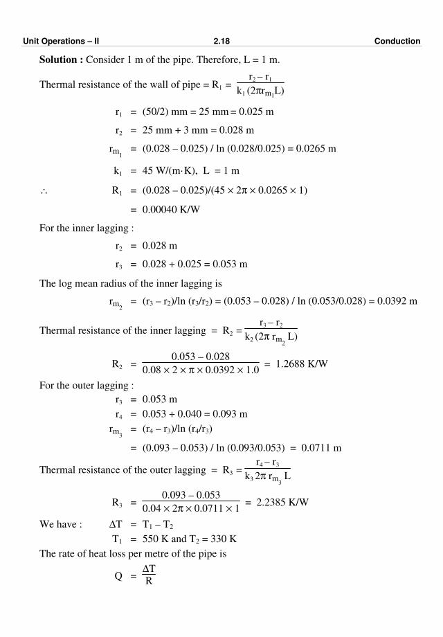
Unit Operations – II 2.18 Conduction
Solution : Consider 1 m of the pipe. Therefore, L = 1 m.
Thermal resistance of the wall of pipe = R1 = r2 – r1
k1 (2πrm1L)
r1 = (50/2) mm = 25 mm = 0.025 m
r2 = 25 mm + 3 mm = 0.028 m
rm1 = (0.028 – 0.025) / ln (0.028/0.025) = 0.0265 m
k1 = 45 W/(m·K), L = 1 m
∴ R1 = (0.028 – 0.025)/(45 × 2π × 0.0265 × 1)
= 0.00040 K/W
For the inner lagging :
r2 = 0.028 m
r3 = 0.028 + 0.025 = 0.053 m
The log mean radius of the inner lagging is
rm2 = (r3 – r2)/ln (r3/r2) = (0.053 – 0.028) / ln (0.053/0.028) = 0.0392 m
Thermal resistance of the inner lagging = R2 = r3 – r2
k2 (2π rm2 L)
R2 = 0.053 – 0.028
0.08 × 2 × π × 0.0392 × 1.0 = 1.2688 K/W
For the outer lagging :
r3 = 0.053 m
r4 = 0.053 + 0.040 = 0.093 m
rm3 = (r4 – r3)/ln (r4/r3)
= (0.093 – 0.053) / ln (0.093/0.053) = 0.0711 m
Thermal resistance of the outer lagging = R3 = r4 – r3
k3 2π rm3 L
R3 = 0.093 – 0.053
0.04 × 2π × 0.0711 × 1 = 2.2385 K/W
We have : ∆T = T1 – T2
T1 = 550 K and T2 = 330 K
The rate of heat loss per metre of the pipe is
Q = ∆T
R
Unit Operations – II 2.19 Conduction
= 550 – 330
0.0004 + 1.2688 + 2.2385
= 62.7 W/m … Ans.
Example 2.9 : A wall of 0.5 m thickness is constructed using a material having a
thermal conductivity of 1.4 W/(m·K). The wall is insulated with a material having thermal
conductivity of 0.35 W/(m·K) so that heat loss per m2 is 1500 W. The inner and outer
temperatures are 1273 K (1000 oC) and 373 K (100 oC) respectively. Calculate the thickness
of insulation required and temperature of the interface between two layers.
Solution : Let the thickness of insulation required be x2 metres.
Given : T1 = 1273 K, T2 = 373 K, k1 = 1.4 W/(m·K), k2 = 0.35 W/(m·K), x1 = 0.5 m
The rate of heat transfer per unit area is given by
Q
A =
(T1 – T2)
x1/k1 + x2/k2
1500 = (1273 – 373)
0.5/1.4 + x2/0.35
Solving, we get
x2 = 0.085 m = 85 mm
Thickness of insulation required = 85 mm … Ans.
Let T' be the temperature at the interface.
Q
A = T1 – T'/(x1/k1)
1500 = (1273 – T')/(0.5/1.4)
T' = 737.3 K (464.3 oC) … Ans.
Example 2.10 : A cylindrical tube has inner diameter of 20 mm and outer diameter of
30 mm. Find out the rate of heat flow from tube of length 5 m if inner surface is at
373 K (100o C) and outer surface is at 308 K (35o C). Take the thermal conductivity of tube
material as 0.291 W/(m·K).
Solution : Basis : Tube of length 5 metres.
The equation to be used for calculating the rate of heat flow through the tube (cylinder) is
Q = k · 2π rm L (T1 – T2)
(r2 – r1) ... (Α)
where, Thermal conductivity = k = 0.291W/(m·K)
Length = L = 5 metres
Inner radius = r1 = 10 mm = 0.01 m
Unit Operations – II 2.20 Conduction
Outside radius = r2 = 15 mm = 0.015 m
Inside temperature = T1 = 373 K
Outside temperature = T2 = 308 K
rm = log mean radius = r2 – r1
ln r2
r1
= 0.015 – 0.01
ln
0.015
0.01
= 0.0123 m
Putting the values of the terms involved in Equation (A), we get
Q = 0.291 × 2π (0.0123) × 5 (373 – 308)
(0.015 – 0.01)
= 1460.8 W ≡ 1460.8 J/s … Ans.
Example 2.11 : 88 mm O.D. pipe is insulated with a 50 mm thickness of an insulation
having a mean thermal conductivity of 0.087 W/(m·K) and 30 mm thickness of an insulation,
having mean thermal conductivity of 0.064 W/(m·K). If the temperature of the outer surface
of the pipe is 623 K (350 oC) and the temperature of the outer surface of insulation is
313 K (40 oC), calculate the heat loss per metre of pipe.
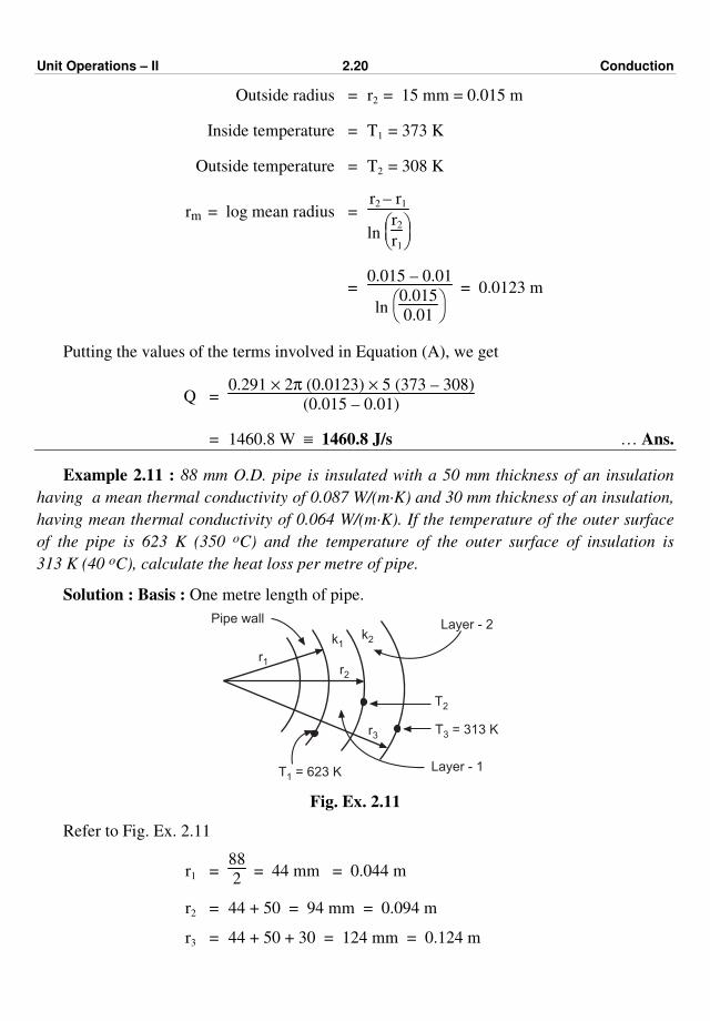
Solution : Basis : One metre length of pipe.
Pipe wall
Layer - 1
Layer - 2
r1
k1k2
r2
r3
T2
T = 313 K3
T = 623 K1
Fig. Ex. 2.11
Refer to Fig. Ex. 2.11
r1 = 88
2 = 44 mm = 0.044 m
r2 = 44 + 50 = 94 mm = 0.094 m
r3 = 44 + 50 + 30 = 124 mm = 0.124 m
Unit Operations – II 2.21 Conduction
Rate of heat flow through a thick-walled cylinder of radii r1 and r2 is given by
Q = k1 (2π rm1
L) (T1 – T2)
(r2 – r1)
∴ Q = T1 – T2
r2 – r1
k1 (2π rm1 L)
… general equation for cylinder.
Similarly, the heat loss through the combined insulation layers is given by
Q = T1 – T3
r2 – r1
k1 (2π rm1 L)
+ r3 – r2
k2 (2π rm2 L)
… (A)
[Q1 = ∆T1/R1
Q2 = ∆T2/R2
∆T1 = Q1R1 and ∆T2 = Q2R2
∆T = ∆T1 + ∆T2
∆T = Q1R1 + Q2R2
But Q1 = Q2 = Q
∴ ∆T = Q [R1 + R2]
Q = ∆T
R1 + R2 =
T1 – T3
R1 + R2]
As T1 – T3 = ∆T = (T1 – T2) + (T2 – T3)
where, ∆T = overall temperature drop
T1 = temperature at the outer surface of the wall = 623 K
T3 = temperature at the outer surface of the outer insulation = 313 K
k1 = thermal conductivity of insulation-1 = 0.087 W/(m·K)
k2 = thermal conductivity of insulation-2 = 0.064 W/(m·K)
L = Length of pipe = 1 metre
rm1 = log mean radius of insulation layer-1
∴ rm1 =
r2 – r1
ln r2
r1
= (0.094 – 0.044)
ln
0.094
0.044
= 0.066 m
Unit Operations – II 2.22 Conduction
rm2 = log mean radius of insulation layer - 2
rm2 = r3 – r2
ln r3
r2
= 0.124 – 0.094
ln
0.124
0.094
= 0.1083 m
Substituting the values of all terms involved in Equation (A), we get
The heat loss per metre of pipe is
Q = (623 – 313)
0.05
0.087 × 2π × 0.066 × 1 +
0.03
0.064 × 2π × 0.1083
Q = 149.4 W/m ………… Ans.
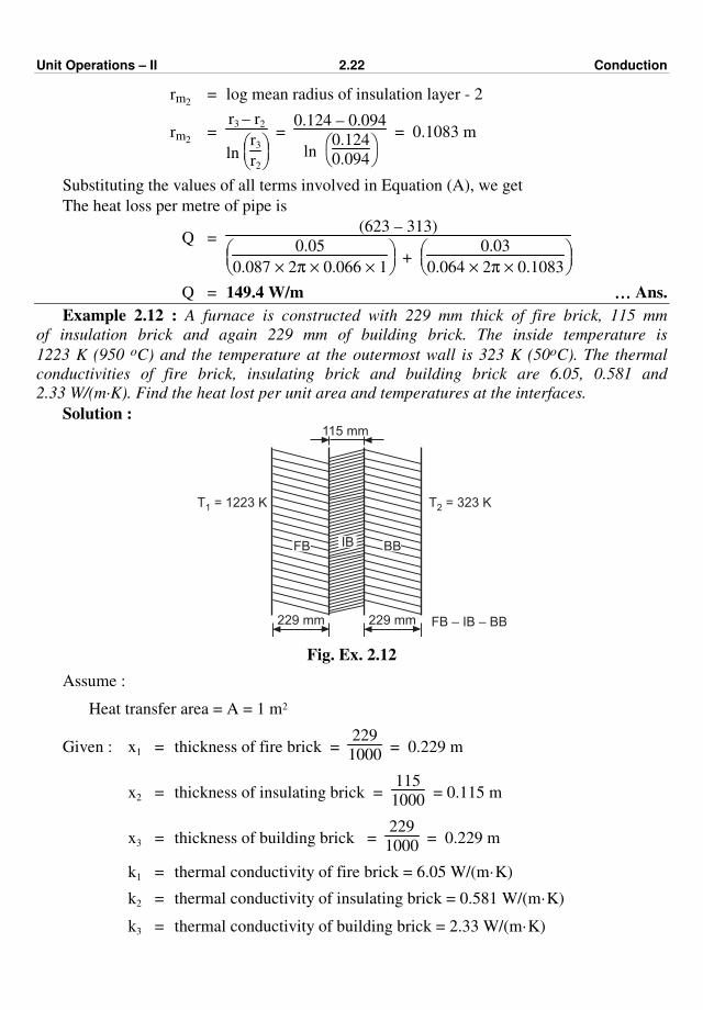
Example 2.12 : A furnace is constructed with 229 mm thick of fire brick, 115 mm
of insulation brick and again 229 mm of building brick. The inside temperature is
1223 K (950 oC) and the temperature at the outermost wall is 323 K (50oC). The thermal
conductivities of fire brick, insulating brick and building brick are 6.05, 0.581 and
2.33 W/(m·K). Find the heat lost per unit area and temperatures at the interfaces.
Solution :
229 mm 229 mm FB – IB – BB
FB BB
T =1 1223 K T =2 323 K
115 mm
IB
Fig. Ex. 2.12
Assume :
Heat transfer area = A = 1 m2
Given : x1 = thickness of fire brick = 229
1000 = 0.229 m
x2 = thickness of insulating brick = 115
1000 = 0.115 m
x3 = thickness of building brick = 229
1000 = 0.229 m
k1 = thermal conductivity of fire brick = 6.05 W/(m·K)
k2 = thermal conductivity of insulating brick = 0.581 W/(m·K)
k3 = thermal conductivity of building brick = 2.33 W/(m·K)
Unit Operations – II 2.23 Conduction
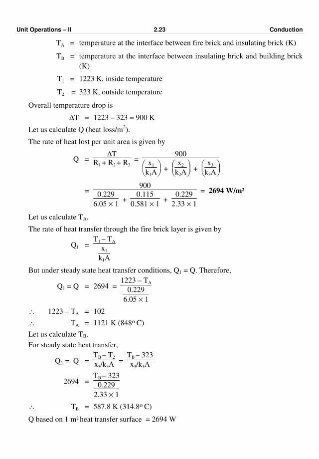
TA = temperature at the interface between fire brick and insulating brick (K)
TB = temperature at the interface between insulating brick and building brick
(K)
T1 = 1223 K, inside temperature
T2 = 323 K, outside temperature
Overall temperature drop is
∆T = 1223 – 323 = 900 K
Let us calculate Q (heat loss/m2).
The rate of heat lost per unit area is given by
Q = ∆T
R1 + R2 + R3 =
900
x1
k1A +
x2
k2A +
x3
k3A
= 900
0.229
6.05 × 1 +
0.115
0.581 × 1 +
0.229
2.33 × 1
= 2694 W/m2
Let us calculate TA.
The rate of heat transfer through the fire brick layer is given by
Q1 = T1 – TA
x1
k1A
But under steady state heat transfer conditions, Q1 = Q. Therefore,
Q1 = Q = 2694 = 1223 – TA
0.229
6.05 × 1
∴ 1223 – TA = 102
∴ TA = 1121 K (848o C)
Let us calculate TB.
For steady state heat transfer,
Q3 = Q = TB – T2
x3/k3A =
TB – 323
x3/k3A
2694 = TB – 323
0.229
2.33 × 1
∴ TB = 587.8 K (314.8o C)
Q based on 1 m2 heat transfer surface = 2694 W
Unit Operations – II 2.24 Conduction
Interface temperatures :
(i) Between FB – IB = 1121 K (848oC) … Ans.
(ii) Between IB – PB = 587.8 K (314.8oC) … Ans.
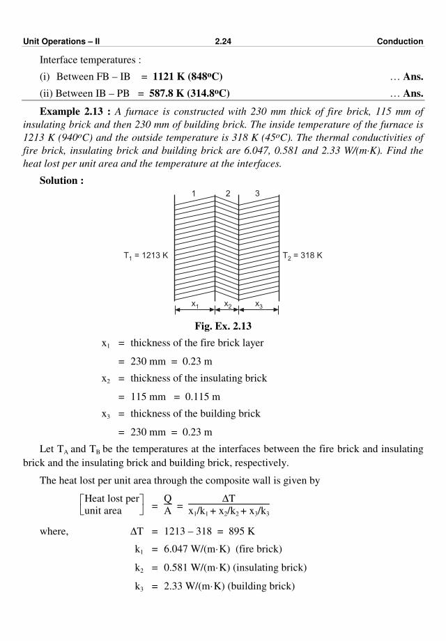
Example 2.13 : A furnace is constructed with 230 mm thick of fire brick, 115 mm of
insulating brick and then 230 mm of building brick. The inside temperature of the furnace is
1213 K (940oC) and the outside temperature is 318 K (45oC). The thermal conductivities of
fire brick, insulating brick and building brick are 6.047, 0.581 and 2.33 W/(m·K). Find the
heat lost per unit area and the temperature at the interfaces.
Solution :
T = 1213 K1
1 2 3
T = 318 K2
x1 x2 x3
Fig. Ex. 2.13
x1 = thickness of the fire brick layer
= 230 mm = 0.23 m
x2 = thickness of the insulating brick
= 115 mm = 0.115 m
x3 = thickness of the building brick
= 230 mm = 0.23 m
Let TA and TB be the temperatures at the interfaces between the fire brick and insulating
brick and the insulating brick and building brick, respectively.
The heat lost per unit area through the composite wall is given by
Heat lost per
unit area = Q
A =
∆T
x1/k1 + x2/k2 + x3/k3
where, ∆T = 1213 – 318 = 895 K
k1 = 6.047 W/(m·K) (fire brick)
k2 = 0.581 W/(m·K) (insulating brick)
k3 = 2.33 W/(m·K) (building brick)
Unit Operations – II 2.25 Conduction
Heat lost per
unit area = 895
0.23
6.047 +
0.115
0.581 +
0.23
2.33
= 2674.2 W ≡ 2674.2 J/s … Ans.
For steady state heat transfer, Q = Q1. Therefore,
∆T
R =
∆T1
R1
∴ ∆T
x1/k1A + x2/k2A + x3/k3A =
∆TA
x1/k1A … for fire brick layer
T1 – T2
x1/k1 + x2/k2 + x3/k3 =
T1 – TA
x1/k1
1213 – 318
0.23
6.047 +
0.115
0.581 +
0.23
2.33
= (1213 – TA)
0.23
6.047
∴ TA = 1108.5 K (835.5 oC) = temperature at the interface between fire brick and
insulating brick. ………… Ans.
Let us calculate the temperature at the interface between insulating brick and building
brick.
For steady state heat transfer, Q = Q3. Therefore,
∆T
R =
∆T3
R3 … for building brick.
(T1 – T2)
x1/k1A + x2/k2A + x3/k3A =
TB – T2
x3/k3A
(T1 – T2)
x1/k1 + x2/k2 + x3/k3 =
TB – T2
x3/k3
1213 – 318
0.23
6.047 +
0.115
0.581 +
0.23
2.33
= TB – 318
0.23
2.33
∴ TB = 565 K (292 oC) = temperature at the interface between the insulating brick and
building brick. ………… Ans.
Example 2.14 : A flat furnace wall is constructed of 45 mm layer of sil-o-cel brick, with a
thermal conductivity of 0.138W/(m·K) backed by a 90 mm layer of common brick of
conductivity 1.38 W/(m·K). Calculate the total thermal resistance considering the area of the
wall as 1m2.
Solution : Basis : Heat transfer area = 1 m2.
Unit Operations – II 2.26 Conduction
x1 = thickness of sil-o-cel brick = 45 mm = 0.045 m
x2 = thickness of common brick = 90 mm = 0.09 m
k1 = thermal conductivity of sil-o-cel brick = 0.138 W/(m·K)
k2 = thermal conductivity of common brick = 1.38 W/(m·K)
A = area of heat transfer = 1 m2
R1 = thermal resistance of the sil-o-cel brick = x1
k1A
R2 = thermal resistance of the common brick = x2
k2A
Total resistance = R = R1 + R2
R = x1
k1A +
x2
k2A =
0.045
0.138 × 1 +
0.09
1.38 × 1 = 0.391 K/W … Ans.
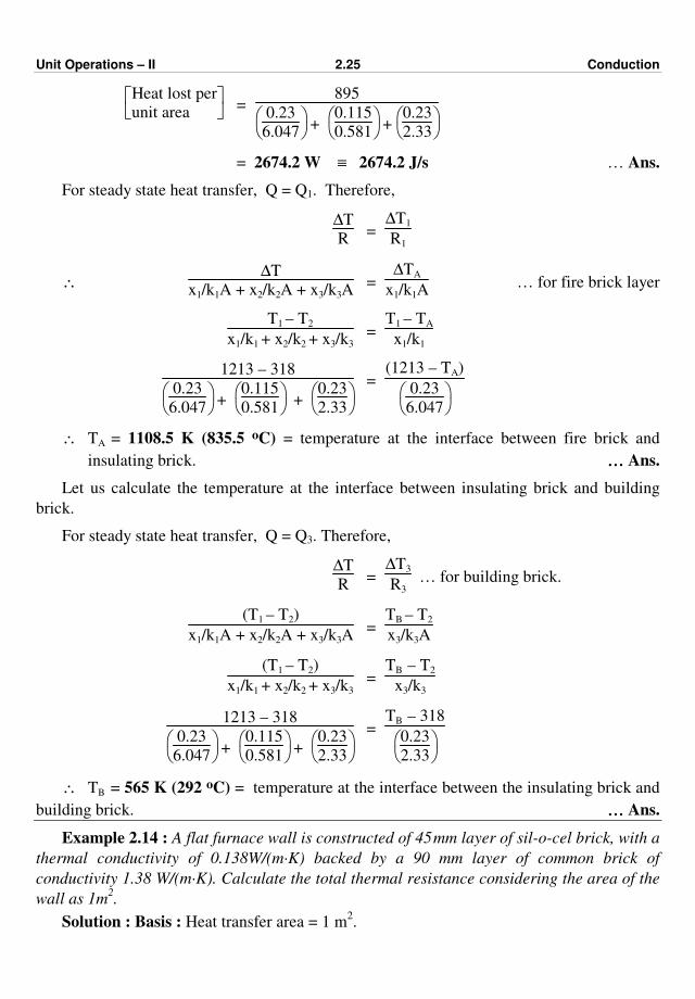
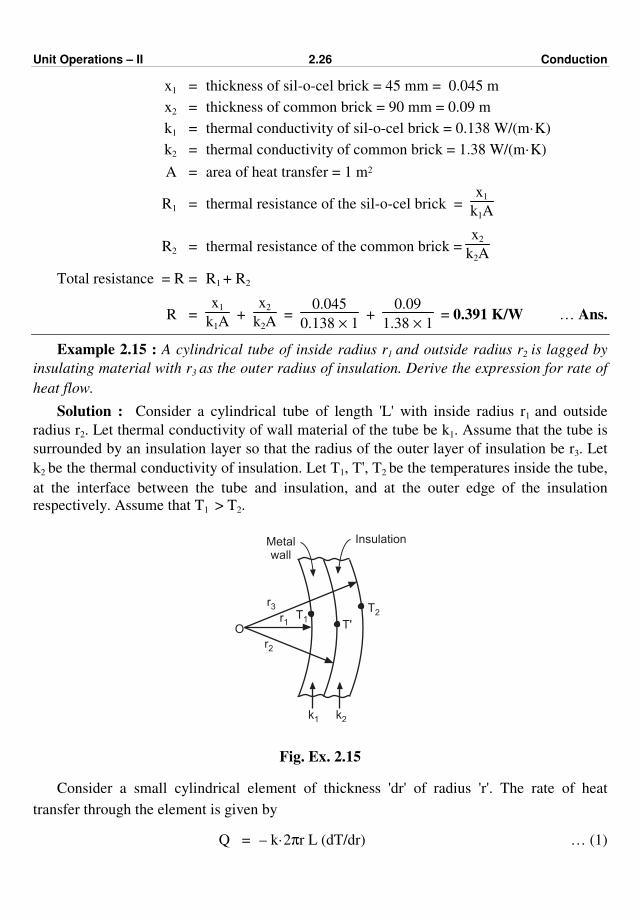
Example 2.15 : A cylindrical tube of inside radius r1 and outside radius r2 is lagged by
insulating material with r3 as the outer radius of insulation. Derive the expression for rate of
heat flow.
Solution : Consider a cylindrical tube of length 'L' with inside radius r1 and outside
radius r2. Let thermal conductivity of wall material of the tube be k1. Assume that the tube is
surrounded by an insulation layer so that the radius of the outer layer of insulation be r3. Let
k2 be the thermal conductivity of insulation. Let T1, T', T2 be the temperatures inside the tube,
at the interface between the tube and insulation, and at the outer edge of the insulation
respectively. Assume that T1 > T2.
Or1
r3
r2
T1
T2
k1 k2
T'
Metalwall
Insulation
Fig. Ex. 2.15
Consider a small cylindrical element of thickness 'dr' of radius 'r'. The rate of heat
transfer through the element is given by
Q = – k·2πr L (dT/dr) … (1)

Unit Operations – II 2.27 Conduction
dr
r =
– k (2π L)
Q dT … (2)
To obtain the rate of heat transfer (Q1) through the tube, the above equation can be
integrated between limits : r = r1, T = T1 and r = r2, T = T'
⌡⌠
r1
r2
dr
r =
– k1 (2πL)
Q1 ⌡⌠
T'
T1
dT … (3)
ln r2
r1 =
k1 (2πL)
Q1 (T1 – T') … (4)
Similarly, for the insulation we can write
ln (r3/r2) ≈ k2 (2πL)
Q2 (T' – T2) … (5)
Rearranging Equations (4) and (5), we get
(T1 – T') = Q1
ln (r2/r1)
k1 (2πL) … (6)
(T' – T2) = Q2
ln (r3/r2)
k2 (2πL) … (7)
Overall temperature drop = ∆T = T1 – T2
(T1 – T2) = (T1 – T') – (T' – T2) … (8)
Substituting for (T1 – T') and (T' – T2) from Equations (6) and (7) into Equation (8), we
get
(T1 – T2) = Q1
ln (r2/r1)
k1 (2πL) + Q2
ln (r3/r2)
k2 (2πL) … (9)
At steady state, Q1 = Q2 = Q, i.e., whatever the heat passes through the tube must pass
through the insulation.
∴ (T1 – T2) = Q
ln (r2/r1)
k1 (2πL) +
ln (r3/r2)
k2 (2πL) … (10)
Q = (T1 – T2)
ln (r2/r1)
k1 (2πL) +
ln (r3/r2)
k2 (2πL)
… (11)
Let rm1 be the log mean radius of the tube.
rm1 = r2 – r1
ln (r2 – r1) … (12)
Unit Operations – II 2.28 Conduction
∴ ln (r2/r1) = r2 – r1
rm1
… (13)
Let rm2 be the log mean radius of the insulation layer.
∴ rm2 = r3 – r2
ln (r3/r2) … (14)
∴ ln (r3 /r2) = r3 – r2
rm2
… (15)
Substituting for ln (r2/r1) and ln (r3/r2) from Equations (13) and (15), Equation (11)
becomes
Q = T1 – T2
(r2 – r1)
k1 2π rm1 L
+ (r3 – r2)
k2 2π rm2 L
Example 2.16 : A flat furnace wall is constructed of 114 mm layer of Sil-o-cel brick,
with a thermal conductivity of 0.138 W/(m·K) backed by 229 mm layer of common brick, of
conductivity 1.38 W/(m·K). The temperature of inner face of wall is 1033 K (760 oC) and that
of the outer face is 349 K (76 oC).
(a) What is the heat loss through the wall ?
(b) Supposing that the contact between two brick layers is poor and that a 'contact
resistance' of 0.09 K/W is present what would be the heat loss ?
Solution : Consider the heat transfer area of the wall be 1 m2.
Thermal resistance of the Sil-o-cel brick layer is : R1 = x1/k1A
Given : x1 = 114 mm = 0.114 m, k1 = 0.138 W/(m·K)
∴ R1 = 0.114
0.138 × 1 = 0.826 K/W
Given : x2 = 229 mm = 0.229 m, k2 = 1.38 W/(m·K)
Thermal resistance of the common brick = R2 = x2/k2A = 0.229
1.38 × 1 = 0.166 K/W
We have : ∆T = T1 – T2 = 1033 – 349 = 684 K
The rate of heat loss per 1 m2 of the wall is
Q = ∆T/(R1 + R2) = 684 / (0.826 + 0.166)
= 689.5 W … Ans. (a)
Given : Contact resistance = 0.09 K/W. Therefore,
Total resistance = R = R1 + R2 + Contact resistance
= 0.826 + 0.166 + 0.09
= 1.082 K/W
Unit Operations – II 2.29 Conduction
The rate of heat loss from 1 m2 heat transfer area considering the contact resistance is
Q = ∆T / R = 684 / 1.082
= 632.2 W … Ans. (b)
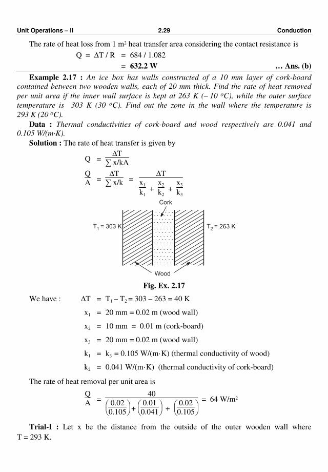
Example 2.17 : An ice box has walls constructed of a 10 mm layer of cork-board
contained between two wooden walls, each of 20 mm thick. Find the rate of heat removed
per unit area if the inner wall surface is kept at 263 K (– 10 oC), while the outer surface
temperature is 303 K (30 oC). Find out the zone in the wall where the temperature is
293 K (20 oC).
Data : Thermal conductivities of cork-board and wood respectively are 0.041 and
0.105 W/(m·K).
Solution : The rate of heat transfer is given by
Q = ∆T
∑ x/kA
Q
A =
∆T
∑ x/k =
∆T
x1
k1 +
x2
k2 +
x3
k3
T = 303 K1 T 263 K2 =
Wood
Cork
Fig. Ex. 2.17
We have : ∆T = T1 – T2 = 303 – 263 = 40 K
x1 = 20 mm = 0.02 m (wood wall)
x2 = 10 mm = 0.01 m (cork-board)
x3 = 20 mm = 0.02 m (wood wall)
k1 = k3 = 0.105 W/(m·K) (thermal conductivity of wood)
k2 = 0.041 W/(m·K) (thermal conductivity of cork-board)
The rate of heat removal per unit area is
Q
A =
40
0.02
0.105 +
0.01
0.041 +
0.02
0.105
= 64 W/m2
Trial-I : Let x be the distance from the outside of the outer wooden wall where
T = 293 K.
Unit Operations – II 2.30 Conduction
For steady state heat transfer,
Q = Qx. Therefore,
∆T
R =
∆T upto x
R upto x
Temperature drop upto a distance x
Total temperature drop =
Rx
R
where Rx = resistance upto a distance x
R = total resistance
Let A = 1 m2
Rx = x
k1 ⋅ A =
x
0.105 × 1 = 0.9524 x K/W
R = 0.02
0.105 × 1 +
0.010
0.041 × 1 +
0.02
0.105 × 1 = 0.625 K/W
303 – 293
40 =
0.9524 x
0.625
Solving, we get
x = 0.0164 m = 16.4 mm … Ans.
∴ Temperature of 293 K (20 oC) will be reached at a point 16.4 mm from the
outermost wall surface of the ice-box.
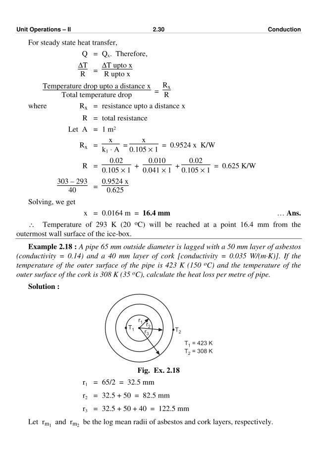
Example 2.18 : A pipe 65 mm outside diameter is lagged with a 50 mm layer of asbestos
(conductivity = 0.14) and a 40 mm layer of cork [conductivity = 0.035 W/(m·K)]. If the
temperature of the outer surface of the pipe is 423 K (150 oC) and the temperature of the
outer surface of the cork is 308 K (35 oC), calculate the heat loss per metre of pipe.
Solution :
T1 T2
r1 r2
r3
T = 423 K
T = 308 K1
2
Fig. Ex. 2.18
r1 = 65/2 = 32.5 mm
r2 = 32.5 + 50 = 82.5 mm
r3 = 32.5 + 50 + 40 = 122.5 mm
Let rm1 and rm2
be the log mean radii of asbestos and cork layers, respectively.
Unit Operations – II 2.31 Conduction
rm1 = r2 – r1
ln r2
r1
= 82.5 – 32.5
ln
82.5
32.5
= 53.7 mm = 0.537 m
rm2 = r3 – r2
ln r3
r2
= 122.5 – 82.5
ln
122.5
82.5
= 101.2 mm = 0.1012 m
r2 – r1 = 82.5 – 32.5 = 50 mm = 0.05 m
r3 – r2 = 122.5 – 82.5 = 40 mm = 0.04 m
∆T = T1 – T2 = 423 – 308 = 115 K
k1 = 0.14 W/(m·K)
k2 = 0.035 W/(m·K)
The rate of heat loss is given by
Q = ∆T
∑ x/kA
Q = ∆T
r2 – r1
k1 2π rm1 L
+ r3 – r2
k2 2π rm2 L
Consider 1 m of the pipe. Therefore,
L = 1 m
The rate of heat loss per meter is
Q = 115
1
2π
0.05
0.14 × 0.0537 × 1 +
0.04
0.035 × 0.1012 × 1
= 40.3 W/m … Ans.
Example 2.19 : A hollow sphere has an inside surface temperature 573 K (300 oC) and
the outside surface temperature 303 K (30 oC). Find the heat loss by conduction for an inside
diameter of 50 mm and outside diameter of 150 mm.
Data : The thermal conductivity of material is 17.45 W/(m·K).
Solution : I.D. of the sphere = 50 mm
∴ r1 = 50
2 = 25 mm = 0.025 m
O.D. of the sphere = 150 mm
r2 = 75 mm = 0.075 m
Unit Operations – II 2.32 Conduction
The rate of heat loss is given by
Q = ∆T ⋅ A
(r2 – r1)/k
A = A1 A2 = 4π r2
1 × 4π r2
2
A = 4π r1 r2
Q = 4π r1 r2 k ∆T
(r2 – r1) =
4π k ∆T
1
r1 –
1
r2
= 4 × π × 17.45 (573 – 303)
1
0.025 –
1
0.075
= 2220 W
∴ Rae of heat loss = Q = 2220 W … Ans.
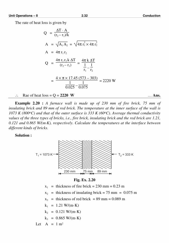
Example 2.20 : A furnace wall is made up of 230 mm of fire brick, 75 mm of
insulating brick and 89 mm of red brick. The temperature at the inner surface of the wall is
1073 K (800oC) and that of the outer surface is 333 K (60oC). Average thermal conductivity
values of the three types of bricks, i.e., fire brick, insulating brick and the red brick are 1.21,
0.121 and 0.865 W/(m·K), respectively. Calculate the temperatures at the interface between
different kinds of bricks.
Solution :
230 mm 75 mm 89 mm
T = 1073 K1 T = 333 K2
Fig. Ex. 2.20
x1 = thickness of fire brick = 230 mm = 0.23 m
x2 = thickness of insulating brick = 75 mm = 0.075 m
x3 = thickness of red brick = 89 mm = 0.089 m
k1 = 1.21 W/(m·K)
k2 = 0.121 W/(m·K)
k3 = 0.865 W/(m·K)
Let A = 1 m2

Unit Operations – II 2.33 Conduction
∑ R = ∑ x/kA
= x1
k1A +
x2
k2A +
x3
k3A
= 0.23
1.21 × 1 +
0.075
0.121 × 1 +
0.089
0.865 × 1
= 0.19 + 0.62 + 0.103 = 0.913 K/W
∆T1 = temperature drop over the fire brick layer
R1 = x1/k1A = 0.23
1.21 × 1 = 0.19 K/W
Let us calculate the temperature at the interface between fire brick and insulating brick.
For steady state heat transfer,
Q = Q1. Therefore,
∆T
∑ R =
∆T1
R1
∆T1
∆T =
R1
∑ R
∆T1 = ∆T × R1
∑ R = (1073 – 333) ×
0.19
0.913 = 154 K
Temperature at the interface between fire brick and insulating brick (T') is
T' = T1 – ∆T1 = 1073 – 154 = 919 K (646oC) … Ans.
Let us calculate the temperature at the interface between insulating brick and red brick.
For steady state heat transfer, Q = Q2. Therefore, ∆T/∑ R = ∆T2/T2.
∆T2
∆T =
R2
∑ R
R2 = x2/k2A = 0.075
0.121 × 1 = 0.62 … Ans.
∆T2 = ∆T × R2
∑ R = (1073 – 333) ×
0.62
0.913 = 502.50 K
Temperature at the interface between insulating brick and red brick (T") is
T" = T' – ∆T2 = 919 – 502.5 = 416.5 K (143.5oC) … Ans.
So the temperatures at the two interfaces are 919 K and 416.5 K.
Example 2.21 : A furnace wall made up of steel plate 10 mm thick lined on the inside
with silica brick 150 mm thick on the outside with magnesite brick 150 mm thick. The
temperature on inside edge of the wall is 973 K (700oC) and on the outside is 288 K (15oC).
Calculate the quantity of heat passed in watts per m2.
It is required to reduce the heat flow to 1163 W/m2 by means of an air gap between steel
plate and magnesite brick. Estimate the width of this gap. Thermal conductivities in W/(m·K)
are 16.86, 1.75, 5.23 and 0.033 respectively for steel, silica brick, magnesite brick and air.

Unit Operations – II 2.34 Conduction
Solution :
Air gapMetalSilica Magnesite
150 mm 10 mm 150 mmw
Fig. Ex. 2.21
w = proposed air gap, m
The rate of heat transfer is given by
Q = ∆T
∑ R
Let the heat transfer area (A) be 1 m2.
Let us calculate the total resistance to heat flow.
∑ R = ∑ x/kA = 0.15
1.75 × 1 +
0.01
16.86 × 1 +
0.15
5.23 × 1 = 0.1153 K/W
… (in the absence of air gap)
Heat flow per 1 m2 area is
Q = ∆T
∑ R =
973 – 288
0.1153 = 5941 W/m2 … (in the absence of air gap)
Let the new resistance be ∑ R' when the heat flow is 1163 W/m2. Therefore,
1163 = ∆T
∑ R'
∑ R' = 973 – 288
1163 = 0.589 K/W
Let w be the width of the air gap.
The total resistance in the presence of air gap is
∑ R' = ∑ R + w
kair × A
= Original resistance + Resistance of air gap
0.589 = 0.1153 + w
0.033 × 1
w = (0.589 – 0.1153) × 0.033 = 0.0156 m = 15.6 mm
Width of the air gap = 15.6 mm … Ans.
Unit Operations – II 2.35 Conduction
Example 2.22 : A 300 mm O.D. pipe is covered with two layers of insulation
[k1 = 0.105 W/(m·K) and k2 = 0.07 W/(m·K)]. The better insulating material is on the outside
and is 40 mm thick. The other insulating material is of 50 mm thickness. The inner and outer
surface temperatures of the insulation are 623 K (350o C) and 323 K (50o C). Estimate :
(a) Heat loss per metre length.
(b) Heat loss per square metre of outer insulation surface.
(c) Temperature of the surface between the two layers of insulation.
Solution : O.D. of pipe = 300 mm
r1 = 300/2 = 150 mm = 0.15 m
r2 = 150 + 50 = 200 mm = 0.20 m
r3 = 200 + 40 = 240 mm = 0.24 m
x1 = 50 mm = 0.05 m
x2 = 40 mm = 0.04 m
The log mean radius of the other insulating material is
rm1 =
r2 – r1
ln r2
r1
= 0.2 – 0.15
ln
0.2
0.15
= 0.1738 m = 0.174 m
The log mean radius of the better insulating material is
rm2 =
r3 – r2
ln r3
r2
= (0.24 – 0.20)
ln
0.24
0.20
= 0.2194 m ~– 0.22 m
The respective thermal resistances are :
R1 = x1
k1A =
0.05
0.105 × π × 0.174 × L =
0.827
L
R2 = x2
k2A =
0.04
0.07 × π × 0.22 × L =
0.827
L
(a) The rate of heat loss per unit length is
Q = ∆T
R1 + R2 =
∆T
0.871
L +
0.827
L
Q
L =
∆T
0.871 + 0.827 =
623 – 323
1.698 = 176.7 W/m
Q
L = 176.7 W/m … Ans. (a)
Unit Operations – II 2.36 Conduction
(b) Perimeter of outer insulation :
= 2π
O.D.
2 + x1 + x2
= 2π (0.15 + 0.05 + 0.04) = 1.508 m
The rate of heat loss per m2 of outer insulation surface is :
Q/L
Perimeter =
Q
L ⋅ perimeter =
176.7
1.508 = 117.2 W/m2 … Ans. (b)
∆T1 = temperature drop over the first insulation
R1 = resistance of the first insulation
= x1
k1A =
0.871
L
Similarly, the overall resistance is
∑ R = 0.871
L +
0.827
L =
1.698
L
For steady state heat transfer, Q = Q1. Therefore, ∆T/R = ∆T1/R1.
∴ ∆T1
∆T =
R1
∑ R
∆T1 = ∆T × R1 / ∑ R
∆T1 = (623 – 323) × 0.871
L × 1.698
L
= 153.9 K
Temperature of the surface between the two layers of insulations (T') is
T' = T1 – ∆T1 = 623 – 153.9 = 469.1 K (196.1o C) … Ans.
Example 2.23 : Estimate the heat loss per m2 of surface area for a furnace wall, 300 mm
thick. The inner and outer surface temperatures are 593 K (320o C) and 311 K (38o C)
respectively. The variation in thermal conductivity (W/(m·K)) with temperature in K is given
by the following relation :
Solution : k = 0.003 T – 10–6 T2
The rate of heat transfer, i.e., the rate of heat loss is given by
Q = – kA dT/dx
Given : k = 0.003 T – 1 × 10⁻⁶ T2
Q ⌡⌠0
x
dx = – A ⌡⌠T1
T2
(0.003 T – 10–6 T2) dT
Unit Operations – II 2.37 Conduction
Q·x = A ⌡⌠T2
T1
(0.003 T – 10–6 T2) dT
Q = A
x
0.003
2 ( )T
2
1 – T2
2 – 10–6
3 ( )T
3
1 – T3
2
Assuming area of heat transfer to be 1 m2.
A = 1 m2
x = 30 cm = 0.3 m
T1 = 593 K
T2 = 311 K
The rate of heat loss per 1 m2 area is
Q = 1
0.3
0.003
2 ( )(593)2 – (311)2 –
10–6
3 ( )(593)3 – (311)3
= 1274.4 W/m2
………… Ans.
Example 2.24 : Calculate the rate of increment of the thickness of an ice layer on the
lake when the thickness of ice is 200 mm and air temperature 263 K. Thermal conductivity of
ice is 1.675 W/(m·K) and density of ice is 900 kg/m3. Take the latent heat of ice as 335 kJ/kg.
Calculate also the time to double the thickness of ice.
Solution : Considering conduction through 1 m2 area of the slab of ice, heat required to
be conducted through the ice to increase the layer thickness by x mm is given by
Q = mλ = A ⋅ x
1000 × λ = 1 ×
x
1000 × 900 × 335 = 301.5 x kJ
Thus, 301.5 x kJ is required to be conducted through 1 m2 area of ice of the average
thickness of 0.20 + x
1000 × 2 = (0.20 + 0.0005 x) m in say t hours.
The rate of heat conducted is
heat to be conducted
t =
– kAdT
dx
heat to be conducted = 301.5 x kJ = 301.5 x × 103 J
(–dT) = – (263 – 273) = 10 K
∴ 301.5 x × 103 = – kA dT
0.20 + 0.0005x m × t
= 1.675 × 1 × 10
0.20 + 0.0005x × t
when t = 1 hr = 3600 s
We have : 301.5 x × 103 = 1.675 × 1 × 10
0.20 + 0.0005x × 3600
∴ x (0.20 + 0.0005x) = 0.20

Unit Operations – II 2.38 Conduction
If x = 1, L.H.S. becomes approximately equal to R.H.S.
Rate of increment
of the thickness of ice = x
t =
1 mm
1 h = 1 mm/h
Original thickness = 200 mm
Time required to double
the thickness of ice = original thickness
rate of increase =
200 mm
1 mm/h = 200 h … Ans.
Example 2.25 : The inside and outside temperature of a furnace wall 300 mm thick of
refractory brick [k = 1.57 W/(m·K)] are at 1923 K (1650 oC) and 593 K (320 oC)
respectively. Find the reduction in heat loss through the wall to be obtained by adding
300 mm thickness of insulating bricks having k = 0.35 W/(m·K) assuming the inside surface
temperature of the refractory bricks to remain fixed at 1923 K (1650 oC). The temperature of
outside surface of the brick may be taken as 300 K (27 oC).
Solution : The rate of heat transfer is given by
Q = k·A (T1 – T2)
x
where k = 1.57 W/(m·K)
x = 300 mm = 0.3 m
Let the area of heat transfer to be 1 m2.
A = 1 m2
T1 = 1923 K
T2 = 593 K
Case-I : The rate of heat loss per 1 m2 area is
Q1 = 1.57 × 1 × (1923 – 593)
0.3 = 6960 W/m
2
Case-II : Heat loss after adding insulating bricks layer. The rate of heat loss per 1 m2
area is
Q2 = A (T1 – T
'2)
x1/k1 + x2/k2
x1 = 0.3 m
x2 = 0.3 m
k1 = 1.57 W/(m·K)
k2 = 0.35 W/(m·K)
T'2 = 300 K
T1 = 1923 K
Q2 = 1 × (1923 – 300)
0.3
1.57 +
0.3
0.35
= 1548 W/m2
Reduction in heat loss per 1 m2 of heat is
Q1 – Q2 = 6960 – 1548 = 5412 W/m2 … Ans.

Unit Operations – II 2.39 Conduction
Example 2.26 : A cold room has one of the walls which measures 4.6 m × 2.3 m
constructed of bricks, 115 mm thick, insulated by cork slabbing 75 mm thick. The cork is
protected externally by wood 25 mm thick. Estimate the leakage through the wall per
24 hours if the interior temperature is 271 K and the exterior 291 K. The thermal
conductivities of brick, cork and wood are 0.113, 0.005 and 0.021 W/(m·K) respectively.
Solution : The rate of heat leakage is given by
Q = A(T1 – T2)
x1/k1 + x2/k2 + x3/k3
A = 4.6 × 2.3 = 10.58 m2
Q = 10.58 (291 – 271)
0.115
0.113 +
0.075
0.005 +
0.025
0.021
= 12.72 W
The heat leakage per 24 hours is
Q' = Q × time = 12.27 × 3600 × 24 × 10–3
= 1060 kJ … Ans.
Example 2.27 : A furnace wall is made up of a steel plate 10 mm thick, lined on the
inside with silica bricks 150 mm thick, and on the outside with magnesite bricks 150 mm
thick. The temperature on the inside edge of the wall is 973 K (700 oC) and on the outside is
423 K (150 oC). Calculate the quantity of heat passed in W/m2 and temperature at the
interface of steel and magnesite brick. Thermal conductivity of steel, silica brick and
magnesite brick are 16.86, 1.75 and 5.23 W/(m·K) respectively.
It is required that the heat flow be reduced to 1163 W/m2 by means of an air gap between
the steel and magnesite brick. Find the width of air gap, if k for air is 0.0337 W/(m·K).
Solution : The rate of heat flow is given by
Q = (T1 – T2)
∑ x/kA
where ∑ x/kA = x1
k1A +
x2
k2A +
x3
k3A
x1 = 10 mm = 0.01 m
x2 = 150 mm = 0.15 m
x3 = 150 mm = 0.15 m
k1 = 16.86 W/(m·K)
k2 = 1.75 W/(m·K)
k3 = 5.23 W/(m·K)

Unit Operations – II 2.40 Conduction
Let the heat transfer area be 1 m2.
∑ x/kA = 0.010
16.86 × 1 +
0.15
1.75 × 1 +
0.15
5.23 × 1 = 0.115 K/W
Q = Heat flow = (973 – 423)
0.115 = 4782.6 W/m2
At steady state, Q passing through the magnesite brick = Q.
∴ Temperature drop in the magnesite bricks
= x3 ⋅ Q
k3 = 4782.6 ×
0.15
5.23 = 137.2 K
∴ Interface temperature between steel and magnesite brick (T") is
T" = T2 + ∆T" = 423 + 137.2 = 560.2 K
∑ x/k with a air gap for reducing the heat loss to 1163 W per m2 is
∑ x/k = ∆T/(Q/A) = A ∆T/Q = 1 × (973 – 423)
1163 = 0.473
∴ x/k for air = 0.473 – 0.115 = 0.358 m2⋅K/W
∴ Air gap thickness = (x/k) × k
= 0.358 × 0.0337 = 0.01206 m
= 12.06 mm … Ans.
Example 2.28 : A steam pipe 115 mm outside diameter, is covered with two layers of
different materials. The first layer is 50 mm thick and has a thermal conductivity of
0.062 W/(m·K). The second layer is 30 mm thick and has a thermal conductivity of
0.872 W/(m·K).
Outside surface temperature of the steam pipe is 508 K (235 oC) and that of the outer
surface of the lagging is 311 K (38 oC). Calculate the heat loss per metre length of the pipe
and the temperature between the two layers of insulation.
Solution : The rate of heat loss is given by
Q = 2πL (T1 – T2)
ln (r2/r1)
k1 +
ln (r3/r2)
k2
where, T1 = 508 K
T2 = 311 K
r1 = 115/2 = 57.5 mm = 0.0575 m
r2 = 57.5 + 50 = 107.5 mm = 0.1075 m
r3 = 107.5 + 30 = 137.5 mm = 0.1375 m
k1 = 0.062 W/(m·K)
k2 = 0.872 W/(m·K)
Unit Operations – II 2.41 Conduction
Consider 1 m of the steam pipe.
L = 1 m
The rate of heat loss per 1 m of the steam pipe is
Q = 2π × 1 (508 – 311)
ln
0.1075
0.0575
0.062 +
ln
0.1375
0.1075
0.872
= 119.3 W/m … Ans.
Let T be the temperature between two layers of insulation.
At steady state, the rate of heat flow through the first layer is the same as Q. Therefore,
Q = 2πL (T1 – T)
ln (r2/r1)
k1
119.3 = 2π × 1 (508 – T)
ln
0.1075
0.0575
0.062
Solving for T, we get
T = 316.4 K (43.4oC) … Ans.
Example 2.29 : A steel pipe with an outside diameter of 115 mm and a wall thickness of
5 mm is covered with 50 mm thickness of 85% magnesia. The surface temperature on the
inside of the pipe is 423 K (150 oC) and that on the outside of insulation is 305 K (32 oC).
Calculate :
(i) The heat flow per metre of length.
(ii) The temperature at the outer surface of the steel pipe and
(iii) The conductance of the pipe and insulation based on its inside surface area.
k for steel = 43.03 W/(m·K)
k for insulation = 0.07 W/(m·K)
Solution : The rate of heat flow is given by
Q = 2πL (T1 – T2)
∑ ln (r2/r1)
k
= 2πL (T1 – T2)
ln (r2/r1)
k1 +
ln (r3/r2)
k2
Consider 1 m of the steel pipe.
L = 1 m, T1 = 423 K, T2 = 305 K, k = 43.03 W/(m⋅K)

Unit Operations – II 2.42 Conduction
r1 = 115 – 2 × 5
2 = 52.5 mm = 0.0525 m
r2 = 115
2 = 57.5 mm = 0.0575 m
r3 = 115
2 + 50 = 107.5 mm = 0.1075 m
The rate of heat loss per 1 m of the steel pipe is
Q = 2π × 1 × (423 – 305)
ln
0.0575
0.0525
43.03 +
ln
0.1075
0.0575
0.07
= 82.92 W/m … Ans. (a)
Let T be the temperature at the outer surface of the steel pipe.
For the steel pipe, at steady state, Q through it is the same as that through the pipe +
insulation. Therefore,
Q = 2πL (T1 – T)
ln (r2/r1)
k
82.92 = 2π × 1 × (423 – T)
ln
0.0575
0.0525
43.03
Solving for T, we get
T = 422.97 K (149.97 oC) … Ans. (b)
This shows that there is a negligible temperature drop over the steel pipe thickness. Thus,
the resistance of the pipe material is negligible as compared with that of the insulation.
As the inside diameter is 105 mm, inside area per metre of the pipe length is
π × 0.105 × 1 = 0.335 m2
Thus, the conductance per 1 m length based on the inside area is
C = 1
R =
Q
A (T1 – T2)
= 82.92
0.335 (423 – 305) = 2.1 W/K
∴ C = 2.1 W/K … Ans. (c)

Unit Operations – II 2.43 Conduction
Example 2.30 : A steam pipe 100 mm outside diameter is covered with two layers of
insulating material, each 25 mm thick, the thermal conductivity of one being three times that
of the other.
Working from first principles show that the effectivity of the two layers is 15.7% less
when the better insulating material is on the inside than when it is on the outside. Assume the
same overall temperature difference in both the cases.
Solution : Consider a thick cylinder of length L. Let k be the thermal conductivity of the
cylinder material. Further consider an element of thickness dr at a radius r concentric with
the cylinder.
The rate of heat transfer through this elementary layer of thickness dr at radius r is
Q = – k 2πrL dT/dr
Integrating between the limits : at r = r1, T = T1 and at r = r2, T = T2
Q ⌡⌠
r1
r2
dr r = – 2πL k ⌡⌠T1
T2
dT
Q ln (r2/r1) = 2πL k (T1 – T2)
Q = 2πL k (T1 – T2)
ln (r2/r1)
Q = 2πL (T1 – T2)
ln (r2/r1)
k
For a composite cylinder, we have
Q = 2πL (T1 – T2)
∑ ln (r2/r1)
k
Let the thermal conductivity of the better insulating material be k.
Thermal conductivity of the outer insulating material = 3 k.
Case-I : Better insulating material on the inside. For this, the rate of heat transfer is given
by
Q1 = 2πL (T1 – T2)
ln (r2/r1)
k +
ln (r3/r2)
3k
where r1 = 100/2 = 50 mm = 0.05 mm
r2 = 50 + 25 = 75 mm = 0.075 m
r3 = 75 + 25 = 100 mm = 0.10 m
Q1 = 2πL (T1 – T2)
ln
0.075
0.050
k +
ln
0.10
0.075
3k
Unit Operations – II 2.44 Conduction
Case-II : Better insulating material on the outside. For this, the rate of heat transfer is
given by
Q2 = 2πL (T1 – T2)
ln (r2/r1)
3k +
ln (r3/r2)
k
= 2πL (T1 – T2)
ln
0.075
0.05
3k +
ln
0.10
0.075
k
Dividing Q1 by Q2 gives
Q1
Q2 =
1/3 ln (3/2) + ln (4/3)
ln (3/2) + 1/3 ln (4/3)
= 0.843. It can be written as : 1 – 0.157
∴ By applying the better insulating material on the inside, the heat conducted is
reduced by 15.7% than that conducted when it is applied on the outside.
∴ Q1 = 0.843 Q2 = (1 – 0.157) Q2 ………… Ans.
Example 2.31 : A 165 mm external diameter pipe is lagged with a 35 mm thickness of
lagging of which thermal conductivity is 0.041 W/(m·K). The lagging outside temperature is
308 K, and brine temperature at a section inside the pipe is 252 K. Find the rise in
temperature of the brine per metre length at this section, if the brine mass flow rate is
0.32 kg/s. Specific heat of brine is 3.6 kJ/(kg.K).
Solution : Neglecting the thermal resistance of pipe, the rate of heat transfer is given by
Q = 2πL k (T1 – T2)
ln (r2/r1)
T1 = 308 K
T2 = 252 K
r1 = 165 mm = 0.165 m
r2 = 165 + 2 × 35 = 235 mm = 0.235 m
Let L = 1 m
Q = 2π × 1 × 0.041 × (308 – 252)
ln
0.235
0.165
= 40.8 W per metre length of pipe.
Unit Operations – II 2.45 Conduction
Heat gained by the brine = 40.8 W
Rise in temperature
of the brine = ∆T
∆T = Q
.m·Cp
= 40.8
0.32 × 3.6 × 103 = 0.0354 K (0.0354o C)
∆T = 0.0354 K (0.0354o C) … Ans.
Example 2.32 : The inside and outside surface of a hollow sphere at r = r1 and r = r2
(r1 < r < r2) are maintained at temperatures T1 and T2 respectively. The thermal conductivity
varies with temperature as
k = k0 (1 + αT + βT2)
Derive an expression for the heat flow rate Q through the sphere.
Solution : Fourier equation for a sphere is
Q = – kA dT
dr
Q
A dr = – k dT
For sphere : A = 4πr2
k = k0 (1 + α T + β T2)
Substituting the values of A and k we get
Q
4π ⌡⌠
r1
r2
dr
r2 = – k0 ⌡⌠T1
T2
(1 + αT + βT2) dT
Q
4π
– 1
r
r2
r1
= k0 ⌡⌠T2
T1
(1 + αT + βT2) dT
– Q
4π
1
r2 –
1
r1 = k0
(T1 – T2) + α2
( )T2
1 – T2
2 + β3
( )T3
1 – T3
2
Q (r2 – r1)
4π r2 r1
= k0 (T1 – T2)
1 + α2
(T1 + T2) + β3
( )T2
1 + T1 T2 + T2
2
Q = k0 4ππππ r1 r2 (T1 – T2)
r2 – r1
1 + αααα
2 (T1 – T2) +
ββββ
3 ( )T
2
1 + T1 T2 + T2
2
………… Ans.
Unit Operations – II 2.46 Conduction
Example 2.33 : A plane wall with isothermal faces T1 at x = 0 and T2 at x = x has a
thermal conductivity of k = ko (1 + aT). Show that the heat conducted through the wall is
given by
Q = ko A
x
1 + a
2 (T1 + T2) (T1 – T2)
Solution : Fourier's law for heat conduction is
Q = – kA dT/dx
Q dx = – kA dT
k = k0 (1 + aT)
∴ Q ⌡⌠ dx = – k0 A ⌡⌠ (1 + aT) dT
The limits of integration are :
At x = 0, T = T1
At x = x, T = T2
Q ⌡⌠0
x
dx = – k0 A ⌡⌠T1
T2
(1 + aT) dT
Q · x = k0 A ⌡⌠T2
T1
(1 + aT) dT
Integrating, we get
Q = k0 A
x
(T1 – T2) + a
2 ( )T
2
1 – T2
2
Q = k0 A
x
(T1 – T2) + a
2 (T1 + T2) (T1 – T2)
∴ Q = k0 A
x
1 + a
2 (T1 + T2) [T1 – T2] … Ans.
Example 2.34 : An exterior wall of house may be approximated by a 100 mm
layer of a common brick [k = 0.70 W/(m·K)] followed by a 40 mm layer of gypsum
plaster [k = 0.48 W/(m·K)]. What thickness of loosely packed rockwool insulation
[k = 0.065 W/(m·K)] should be added to reduce the heat loss through the wall by 25% ?
Solution : Let the area of heat transfer be 1 m2.
The rate of heat loss is given by
Q = ∆T
∑ x/kA
∑ x/kA = x1
k1A +
x2
k2A

Unit Operations – II 2.47 Conduction
where, x1 = 100 mm = 0.10 m
x2 = 40 mm = 0.04 m
k1 = 0.7 W/(m·K)
k2 = 0.48 W/(m·K) and A = 1 m2
∑ x/kA = 0.10
0.7 × 1 +
0.04
0.48 × 1 = 0.226 K/W
∴ Q = ∆T
0.226 = 4.42 ∆T … (1)
Given : When the rockwool insulation added, the heat loss is reduced by 25% so the heat
loss is 0.75 Q. The rate of heat loss through the new system is
Q' = 0.75 Q
This heat loss is by considering the resistance of rockwool insulation and is given by
Q' = ∆T
∑ x/kA
Q' = ∆T
x1/k1A + x2/k2A + x3/k3A
where, x3 = thickness of rockwool insulation in m
k3 = 0.065 W/(m·K)
Q' = ∆T
0.10
0.7 × 1 +
0.04
0.48 × 1 +
x3
0.065 × 1
… (2)
But Q' = 0.75 Q … (3)
Equating Equations (2) and (3) and substituting the value of Q from Equation (1) gives
0.75 × 4.42 × ∆T = ∆ T
0.226 + x3
0.065
0.75 × 4.42
0.226 +
x3
0.065 = 1
0.7492 + 51 x3 = 1
x3 = 4.92 × 10⁻³ m = 4.92 mm … Ans.
Thickness of the rockwool insulation required = 4.92 mm. … Ans.
Example 2.35 : A steam pipe, 40 mm outside diameter, is to be insulated by two layers of
insulation each 20 mm thick. The material M-1 has thermal conductivity k and the material
M-2 has thermal conductivity 3k. Assuming that the inner and outer surface temperatures of
a composite insulation to be fixed, find which arrangement would give less heat loss rate,
M-1 near the pipe surface and M-2 as the outer layer or vice versa ? Also calculate the
percent reduction in heat loss.

Unit Operations – II 2.48 Conduction
Solution : Arrangement-1 : Let the layer of material M-1 be nearer to the surface of the
steam pipe.
The rate of heat loss is given by
Q1 = T1 – T2
ln r2/r1
2π L k1
+ ln r3/r2
2π L k2
Here, k1 = k and k2 = 3k
r1 = 40/2 = 20 mm = 0.02 m
r2 = 20 + 20 = 40 mm = 0.04 m
r3 = 40 + 20 = 60 mm = 0.06 m
T1 and T2 be the temperatures at the inner surface of the pipe and at the outer surface
insulation.
Q1 = T1 – T2
ln (0.04/0.02)
2π L k +
ln (0.06/0.04)
2π L × 3k
Q1 = T1 – T2
ln 2
2π k +
ln 1.5
6π k
= k L (T1 – T2)
0.1318 = 7.59 kL (T1 – T2)
Arrangement-2 : Let the layer of material M-2 be nearer to the surface of the steam
pipe.
The rate of heat loss is given by
Q2 = T1 – T2
ln r2/r1
2π L k1
+ ln r3/r2
2π L k2
= T1 – T2
ln (0.04/0.02)
2π L × 3k +
ln (0.06/0.04)
2π Lk
= kL (T1 – T2)
ln 2
6π +
ln 1.5
2π
= k L (T1 – T2)
0.1013 = 9.87 kL (T1 – T2)
Unit Operations – II 2.49 Conduction
For any values of k, T1 and T2 , Q1 is always less than Q2 since Q1 is 7.59 times
kL (T1 – T2) and Q2 is 9.87 times kL (T1 – T2)
∴ M-1 near the surface is advisable (i.e., the arrangement-1 will result in less heat loss).
% reduction in
the heat loss = 9.87 kL (T1 – T2) – 7.59 kL (T1 – T2)
9.87 kL (T1 – T2) × 100
= 9.87 – 7.59
9.87 × 100
= 23.1 % … Ans.
Example 2.36 : A steel pipe [k = 50 W/(m·K)] of 100 mm I.D. and 110 mm O.D. is to be
covered with two layers of insulation each having thickness of 50 mm. The thermal
conductivity of the first insulation material is 0.06 W/(m·K) and that of second is
0.12 W/(m·K). Estimate the heat loss per 1 m length of pipe when the temperature of the
inside tube surface is 523 K (250 oC) and that of the outer surface of insulation is
323 K (50 oC).
If the order of insulation material were reversed, i.e., the insulation with higher value of
thermal conductivity was put first, calculate the change in the heat loss with all other
conditions kept unchanged. Comment on results.
Solution : T1 = 523 K, T2 = 323 K
r1 = 100/2 = 50 mm = 0.050 m, r2 = 110/2 = 55 mm = 0.055 m
r3 = 55 + 50 = 105 mm = 0.105 m, r4 = 105 + 50 = 155 mm = 0.155 m
k1 = 50 W/(m·K), k2 = 0.06 W/(m·K)
k3 = 0.12 W/(m·K)
Case I :
First layer of insulation is of the insulation material having k = 0.06 W/(m·K), i.e., of the
material having a lower value of thermal conductivity.
Q
L1
= 2π (T1 – T2)
ln (r2/r1)
k1 +
ln (r3/r2)
k2 +
ln (r4/r3)
k3
= 2π (523 – 323)
ln (0.055/0.05)
50 +
ln (0.105/0.055)
0.06 +
ln (0.155/0.105)
0.12
= 89.9 W/m … Ans.
Case II :
The insulation material of higher thermal conductivity is put first, i.e., near the pipe
surface and the insulation of lower thermal conductivity at the outer layer. In this case,
k2 = 0.12 W/(m·K) and k3 = 0.06 W/(m·K).
Unit Operations – II 2.50 Conduction
Q
L2
= 2π (523 – 323)
ln (0.055/0.05)
40 +
ln (0.105/0.055)
0.12 +
ln (0.155/0.105)
0.06
= 105.75 W/m … Ans.
As (Q/L)1 is less than (Q/L)2, the insulation material having a low thermal conductivity
should be put first, i.e., near the pipe surface.
With the material having a low k value, % reduction in the heat loss is
% reduction in the heat loss = 105.75 – 89.6
89.6 × 100 = 18.02 ………… Ans.
By comparing the results, it is seen that the loss of heat is increased by 18.02% by
applying the insulation material with a higher thermal conductivity near the pipe surface. As
the purpose of insulation is to reduce the heat loss, it is always better to provide the
insulating material with a low thermal conductivity on the surface of pipe first, i.e., near the
pipe surface.
Example 2.37 : A steam pipe 10 cm O.D. is to be insulated by two layers of insulations
each 2.5 cm thick. The material 'A' has a thermal conductivity of k and the material 'B' has
conductivity 3 k. Assuming that the inner and outer temperatures of composite insulation to
be fixed, find :
(i) Which arrangement would give less heat loss rate, 'A' near the pipe surface and
'B' as outer layer or vice versa ?
(ii) What is the percent reduction in the heat loss rate ?
Solution : Let T1 be the temperature at the outer surface of pipe and T2 be the
temperature at the outer surface of insulation. These temperatures are fixed in both the
following cases :
Case I : A near the surface.
Case II : B near the surface.
We have Q = (T1 – T2)
ln (r2/r1)
2π k1 L +
ln (r3/r2)
2π k2 L
Consider 1 m of the pipe.
∴ L = 1 m
Case I : 'A' near the pipe surface :
r1 = outer radius of pipe = 100 mm = 0.10 m
r2 = outer radius of inner insulation (A) = 100 + 25 = 125 mm = 0.125 m
r3 = outer radius of outer insulation (B) = 125 + 25 = 150 mm = 0.150 m

Unit Operations – II 2.51 Conduction
k1 = thermal conductivity of 'A' = k, W/(m·K)
k2 = thermal conductivity of 'B' = 3 k, W/(m·K)
∴ Q1 = (T1 – T2)
ln (0.125/0.10)
2π × k × 1.0 +
ln (0.15/0.125)
2π × 3k × 1.0
Q1 = ∆T
0.0355
k +
0.0097
k
= ∆T
0.0452/k = 22.12 k ∆T
Case II : 'B' near the pipe surface :
Q2 = (T1 – T2)
ln (0.125/0.10)
2π × 3k × 1.0 +
ln (0.15/0.125)
2π × k × 1.0
Q2 = ∆T
0.012
k +
0.029
k
= ∆T
0.041
k
= 24.39 k ∆T
Q1 = 22.12 k ∆T and Q2 = 24.39 k ∆T ∴ Q1 is less than Q2, i.e., the arrangement :
'A' near the pipe surface (and 'B' as the outer layer) gives less heat loss. … Ans. (i)
To reduce the heat loss, 'A' near the pipe surface should be used. For reducing the heat
loss, the material having a low thermal conductivity should be always near the pipe surface.
% Reduction in the heat loss
(with A near the pipe surface) = 24.39 k ∆T – 22.12 k ∆T
22.12 k ∆T × 100 = 10.26 … Ans. (ii)
Example 2.38 : A wall of a furnace 0.224 m thick is constructed of a material having a
thermal conductivity of 1.3 W/(m·K). This will be insulated on the outside with material
having an average k of 0.346 W/(m·K) so that the heat loss from the furnace will be equal to
or less than 1830 W/m2. The inner surface temperature is 1588 K (1315 oC) and the outer
299 K (26 oC). Calculate the thickness of insulation required.
Solution : x1 = 0.224 m, k1 = 1.3 W/(m·K)
x2 = ? k2 = 0.346 W/(m·K)
T1 = 1588 K and T2 = 299 K
Q/A = the rate of heat loss per unit area = 1830 W/m2

Unit Operations – II 2.52 Conduction
We have : Q
A =
(T1 – T2)
x1/k1 + x2/k2
1830 (x1/k1 + x2/k2) = (1588 – 299)
x1
k1 +
x2
k2 = 0.7044
0.224
1.3 +
x2
k2 = 0.7044
x2/k2 = 0.5321
x2 = 0.5321 k2 = 0.5321 × 0.346 = 0.184 m = 184 mm
Thickness of the insulation required = 184 mm … Ans.
Example 2.39 : An exterior wall of a house may be approximated by a 100 mm layer of
common brick followed by a 40 mm layer of gypsum plaster. What thickness of loosely
packed rock wool insulation should be added to reduce the heat loss through the wall by
80 percent ?
Data : k for common brick = 0.7 W/(m·K)
k for gypsum layer = 0.48 W/(m·K)
k for rock wool = 0.065 W/(m·K)
Solution : The rate of heat loss is given by
Q = ∆T/∑ R
Q without insulation = Q = ∆T/∑ R
Q with insulation = Q' = ∆T/∑ R'
With rock wool insulation, the heat loss is reduced by 80%.
∴ Heat loss with insulation will be 20% of the heat loss without insulation.
Q' = 0.2, Q = 0.2 ∆T
∑ R =
∆T
∑ R'
∴ Q'
Q = 0.2 =
∑ R
∑ R'
Let the area of heat transfer be 1 m2.
A = 1 m2
x1 = 100 mm = 0.10 m, x2 = 40 mm = 0.04 m
x3 = thickness of rock wool insulation
k1 = 0.7 W/(m·K), k2 = 0.48 W/(m·K), k3 = 0.065 W/(m·K)
Brick : R1 = x1/k1A = 0.1/0.7 × 1 = 0.143 K/W
Plaster : R2 = x2/k2 A = 0.04 /0.48 × 1 = 0.083 K/W
∴ R = R1 + R2 = 0.143 + 0.083 = 0.226 K/W
Unit Operations – II 2.53 Conduction
Rock wool : R3 = x3/k3 A = x3/0.065 × 1 = 15.4 x3 K/W
R' = R1 + R2 + R3 = 0.226 + 15.4 x3
R = Resistance without insulation
R' = Resistance with insulation
∴ 0.2 = 0.226
0.226 + 15.4 x3
Solving for x3, we get
x3 = 0.0587 m = 58.7 mm ≈ 59 mm
Thickness of rock wool insulation = 59 mm. ………… Ans.
Systems with Variable Thermal Conductivity :
Now we will take into account the variation of k with temperature in deriving the heat
flow equations for a plane wall, a cylinder, etc.
Plane wall with variable k :
A plane wall of thickness x has one surface at T1 and the other surface at T2. If the
thermal conductivity of the wall varies with temperature as per the following equation :
k = ko (1 + αT), derive an expression for the heat flow rate, Q.
Solution : The Fourier's equation for heat conduction is
Q = – kA dT/dx
Q dx = kA dT
Given : k = ko (1 + αT)
∴ Q dx = – ko (1 + αT) A dT
The boundary conditions are :
at x = 0, T = T1
and at x = L, T = T2
Integrating within the limits, we get
Q ⌡⌠0
x
dx = – ko A ⌡⌠T1
T2
(1 + αT) dT = ko A ⌡⌠T2
T1
(1 + αT) dT
Qx = ko A
T + α2
T2
T1
T2
Q = ko A
x
(T1 – T2) + α2
( )T2
1 – T2
2
Q = ko A
x (T1 – T2)
1 + α2
(T1 + T2) … (2.50)
Hollow cylinder with variable k :
Consider a hollow cylinder. The inner and outer surfaces of the hollow cylinder are
maintained at uniform temperatures T1 and T2 respectively. The cylinder of length L and r1

Unit Operations – II 2.54 Conduction
and r2 are its the inside and the outside radii, respectively. The thermal conductivity of the
material of cylinder is temperature dependent and given by the equation :
k = ko (1 + αT + βT2)
Derive an expression for the rate of heat flow through the cylinder.
Solution : The Fourier's law of heat conduction is
Q = – kA dT
dr
With k = ko (1 + αT + βT2) it becomes
Q = – ko (1 + αT + βT2) A
dT
dr
Rearranging, we get
Q dr
r = – ko 2πL (1 + αT + βT
2) dT
The boundary conditions are :
at r = r1, T = T1 and at r = r2, T = T2
Integrating within the limits, we get
Q ⌡⌠
r1
r2
dr
r = – ko · 2πL ⌡⌠
T1
T2
(1 + αT + βT2) dT
Q ⌡⌠
r1
r2
dr
r = 2π ko L ⌡⌠
T2
T1
(1 + αT + βT2) dT
Q [ln r]
r2
r1
= 2π ko L
T + α2
T2 + β3
T3
T1
T2
Q ln (r2/r1) = 2π ko L
(T1 – T2) + α2
( )T2
1 – T2
2 + β3
( )T3
1 – T3
2
Q =
2π ko L
(T1 – T2) + α2
( )T2
1 – T2
2 + β3
( )T3
1 – T3
2
ln (r2/r1)
Q = 2π ko L (T1 – T2) [1 + α/2 (T1 + T2) + β/3 (T
2
1 + T1 T2 + T2
2)]
ln (r2/r1)
… (2.51)
Equation (2.51) is the desired expression for the rate of heat flow through a hollow
cylinder.

Unit Operations – II 2.55 Conduction
Hollow sphere with variable k :
Consider a hollow sphere with boundary surfaces at r = r1 and r = r2 maintained at
uniform temperatures T1 and T2, respectively. The thermal conductivity of the material of
sphere varies with temperature, and is given by
k(T) = ko (1 + αT + βT2)
where r1 and r2 are the inner and outer radii of the sphere.
Derive an expression for the heat flow rate Q through the sphere.
Solution : Q = – kA dT/dr = – k 4πr2 dT
dr
∴ Q · dr
r2 = – 4π k dT
Limits for the integration are :
at r = r1, T = T1 and at r = r2, T = T2
k = ko (1 + αT + βT2)
∴ Q ⌡⌠
r1
r2
dr
r2 = – 4π ko ⌡⌠T1
T2
(1 + αT + βT2) dT
– Q 1
r
r2
r1
= 4π ko
T + α2
T2 + β3
T3
T1
T2
– Q
1
r2 –
1
r1 = 4π ko
(T1 – T2) + α2
(T2
1 – T2
2) + β3
(T3
1 – T3
2)
Q
1
r1 –
1
r2 = 4π ko
(T1 – T2) + α2
(T2
1 – T2
2) + β3
(T3
1 – T3
2)
Q
r2 – r1
r1r2 = 4π ko
(T1 – T2) + α2
(T2
1 – T2
2) + β3
(T3
1 – T3
2)
∴ Q = 4π ko · r1r2
(r2 – r1)
(T1 – T2) + α2
(T2
1 – T2
2) + β3
(T3
1 – T3
2)
Q = 4π ko r1r2
(r2 – r1) (T1 – T2)
1 + α2
(T1 + T2) + β3
(T2
1 + T1 T2 + T2
2)
… (2.52)
Equation (2.52) is the desired expression for the heat flow through a sphere.
Critical Radius of Insulation :
It is always necessary to provide insulation on the external surfaces of pipelines and
vessels to reduce the heat loss to the ambient, e.g., steam piping, piping carrying refrigerant,
etc. It is natural to expect that the greater the thickness of insulation, the less will the heat
loss. The following analysis reveals that this may not be always the case.
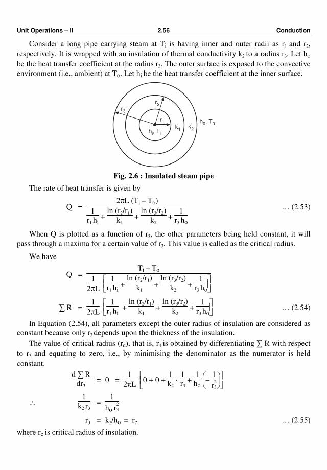
Unit Operations – II 2.56 Conduction
Consider a long pipe carrying steam at Ti is having inner and outer radii as r1 and r2, respectively. It is wrapped with an insulation of thermal conductivity k2 to a radius r3. Let ho
be the heat transfer coefficient at the radius r3. The outer surface is exposed to the convective
environment (i.e., ambient) at To. Let hi be the heat transfer coefficient at the inner surface.
r3
r2
r1
h , Tii
k1k2
h , T00
Fig. 2.6 : Insulated steam pipe
The rate of heat transfer is given by
Q = 2πL (Ti – To)
1
r1 hi +
ln (r2/r1)
k1 +
ln (r3/r2)
k2 +
1
r3 ho
… (2.53)
When Q is plotted as a function of r3, the other parameters being held constant, it will
pass through a maxima for a certain value of r3. This value is called as the critical radius.
We have
Q = Ti – To
1
2πL
1
r1 hi +
ln (r2/r1)
k1 +
ln (r3/r2)
k2 +
1
r3 ho
∑ R = 1
2πL
1
r1 hi +
ln (r2/r1)
k1 +
ln (r3/r2)
k2 +
1
r3 ho … (2.54)
In Equation (2.54), all parameters except the outer radius of insulation are considered as
constant because only r3 depends upon the thickness of the insulation.
The value of critical radius (rc), that is, r3 is obtained by differentiating ∑ R with respect
to r3 and equating to zero, i.e., by minimising the denominator as the numerator is held
constant.
d ∑ R
dr3 = 0 =
1
2πL
0 + 0 + 1
k2 ·
1
r3 +
1
ho
– 1
r2
3
∴ 1
k2 r3 =
1
ho r2
3
r3 = k2/ho = rc … (2.55)
where rc is critical radius of insulation.
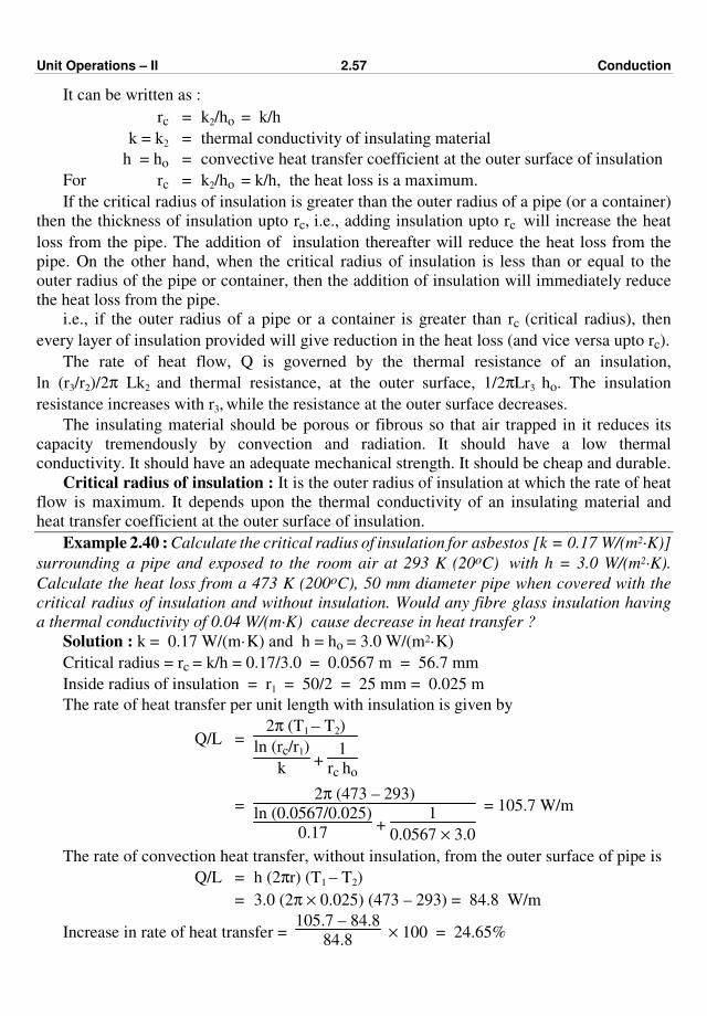
Unit Operations – II 2.57 Conduction
It can be written as :
rc = k2/ho = k/h
k = k2 = thermal conductivity of insulating material
h = ho = convective heat transfer coefficient at the outer surface of insulation
For rc = k2/ho = k/h, the heat loss is a maximum.
If the critical radius of insulation is greater than the outer radius of a pipe (or a container)
then the thickness of insulation upto rc, i.e., adding insulation upto rc will increase the heat
loss from the pipe. The addition of insulation thereafter will reduce the heat loss from the
pipe. On the other hand, when the critical radius of insulation is less than or equal to the
outer radius of the pipe or container, then the addition of insulation will immediately reduce
the heat loss from the pipe.
i.e., if the outer radius of a pipe or a container is greater than rc (critical radius), then
every layer of insulation provided will give reduction in the heat loss (and vice versa upto rc).
The rate of heat flow, Q is governed by the thermal resistance of an insulation,
ln (r3/r2)/2π Lk2 and thermal resistance, at the outer surface, 1/2πLr3 ho. The insulation
resistance increases with r3, while the resistance at the outer surface decreases.
The insulating material should be porous or fibrous so that air trapped in it reduces its
capacity tremendously by convection and radiation. It should have a low thermal
conductivity. It should have an adequate mechanical strength. It should be cheap and durable.
Critical radius of insulation : It is the outer radius of insulation at which the rate of heat
flow is maximum. It depends upon the thermal conductivity of an insulating material and
heat transfer coefficient at the outer surface of insulation.
Example 2.40 : Calculate the critical radius of insulation for asbestos [k = 0.17 W/(m2·K)]
surrounding a pipe and exposed to the room air at 293 K (20oC) with h = 3.0 W/(m2·K).
Calculate the heat loss from a 473 K (200oC), 50 mm diameter pipe when covered with the
critical radius of insulation and without insulation. Would any fibre glass insulation having
a thermal conductivity of 0.04 W/(m·K) cause decrease in heat transfer ?
Solution : k = 0.17 W/(m·K) and h = ho = 3.0 W/(m2·K)
Critical radius = rc = k/h = 0.17/3.0 = 0.0567 m = 56.7 mm
Inside radius of insulation = r1 = 50/2 = 25 mm = 0.025 m
The rate of heat transfer per unit length with insulation is given by
Q/L = 2π (T1 – T2)
ln (rc/r1)
k +
1
rc ho
= 2π (473 – 293)
ln (0.0567/0.025)
0.17 +
1
0.0567 × 3.0
= 105.7 W/m
The rate of convection heat transfer, without insulation, from the outer surface of pipe is
Q/L = h (2πr) (T1 – T2)
= 3.0 (2π × 0.025) (473 – 293) = 84.8 W/m
Increase in rate of heat transfer = 105.7 – 84.8
84.8 × 100 = 24.65%

Unit Operations – II 2.58 Conduction
Therefore, addition of 56.7 – 25 = 31.7 mm of the insulation actually increases the heat
transfer by 24.65%.
Fibre glass insulation, k = 0.04 W/(m2·K)
Critical radius of insulation = rc = k/h = 0.04
3.0 = 0.0133 m ………… Ans.
In this case, the value of critical radius (0.0133 m) is less than the outside radius of the
pipe (0.025 m). Therefore, the addition of any fibre glass insulation would cause a decrease
in the heat transfer.
Critical radius insulation for insulated sphere : For a sphere, we have
Q = ∆T/ ∑ R
Let r1, r2 be the inside and outside radii of sphere, respectively and r3 be the outer radius
of insulation. r2 is also the inner radius of insulation.
Let k1 and k2 be the thermal conductivities of the sphere material and insulation. Let
hi and ho be the heat transfer coefficients on the inside of the sphere and at the outer surface
of the insulation.
Total thermal resistance is given by
∑ R = 1
4π r2
1 hi
+ (r2 – r1)
4π k1 r1 r2
+ r3 – r2
4π k2 r2 r3
+ 1
4π r2
3 · ho
… (2.56)
Differentiating ∑ R (i.e., Equation 2.56) with respect to r3 and equating to zero, we get.
In the above equation only r3 depends upon the insulation provided, so all other
parameters are taken as constant.
d ∑ R
dr3 = 0 =
– 1
4π k2 r2
3
– 2
4π ho r3
3
∴ r3 = 2 k2
ho = rc
∴ Critical radius of insulation for sphere = rc = 2 k2
ho =
2 k
h … (2.57)
where k = k2 = thermal conductivity of insulating material
and h = ho = heat transfer coefficient between the outer surface of
insulation and ambient.
Example 2.41 : Derive a relation for the critical radius of insulation for a circular
cross-section having radius R and length L.
Solution : Consider an insulated pipe of length L with R1 and R2 as its inside and outside
radii, respectively. Let R3 be the outer radius of insulation. Let k1 and k2 be the thermal
conductivities of the pipe material and insulating material respectively. Let hi and ho be the
heat transfer coefficients on the inside surface of the pipe and at the outer surface of
insulation. Then,
Q = (T1 – T2)
∑ R
∑ R = 1
2π R1 L hi +
ln (R2/R1)
2π L k1
+ ln (R3/R2)
2π L k2
+ 1
2π R3 L ho
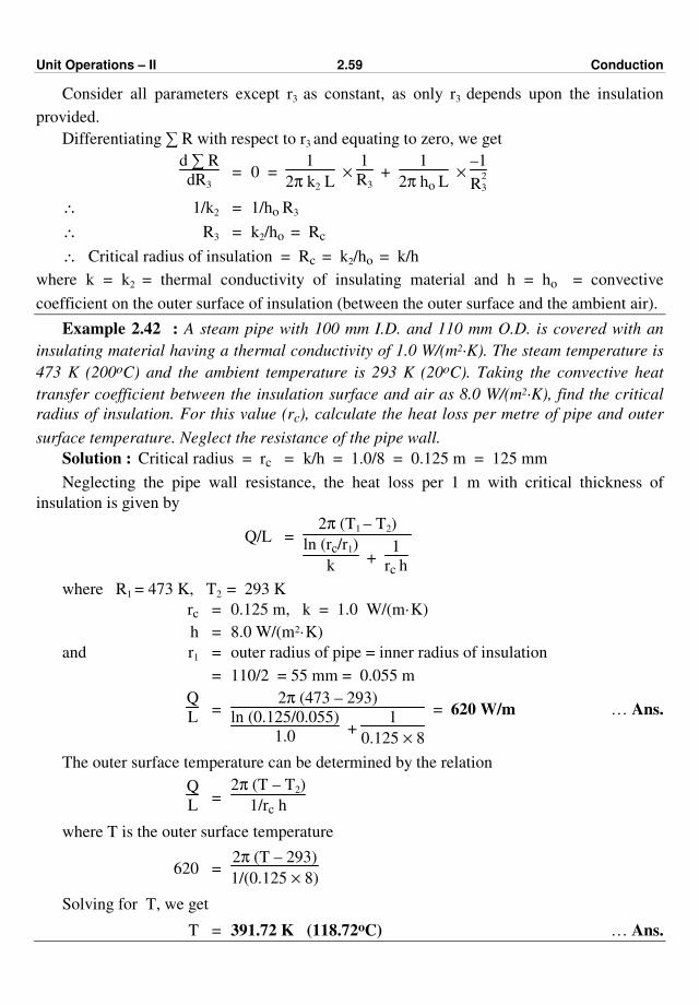
Unit Operations – II 2.59 Conduction
Consider all parameters except r3 as constant, as only r3 depends upon the insulation
provided.
Differentiating ∑ R with respect to r3 and equating to zero, we get
d ∑ R
dR3 = 0 =
1
2π k2 L ×
1
R3 +
1
2π ho L ×
–1
R2
3
∴ 1/k2 = 1/ho R3
∴ R3 = k2/ho = Rc
∴ Critical radius of insulation = Rc = k2/ho = k/h
where k = k2 = thermal conductivity of insulating material and h = ho = convective
coefficient on the outer surface of insulation (between the outer surface and the ambient air).
Example 2.42 : A steam pipe with 100 mm I.D. and 110 mm O.D. is covered with an
insulating material having a thermal conductivity of 1.0 W/(m2·K). The steam temperature is
473 K (200oC) and the ambient temperature is 293 K (20oC). Taking the convective heat
transfer coefficient between the insulation surface and air as 8.0 W/(m2·K), find the critical
radius of insulation. For this value (rc), calculate the heat loss per metre of pipe and outer
surface temperature. Neglect the resistance of the pipe wall.
Solution : Critical radius = rc = k/h = 1.0/8 = 0.125 m = 125 mm
Neglecting the pipe wall resistance, the heat loss per 1 m with critical thickness of
insulation is given by
Q/L = 2π (T1 – T2)
ln (rc/r1)
k +
1
rc h
where R1 = 473 K, T2 = 293 K
rc = 0.125 m, k = 1.0 W/(m·K)
h = 8.0 W/(m2·K)
and r1 = outer radius of pipe = inner radius of insulation
= 110/2 = 55 mm = 0.055 m
Q
L =
2π (473 – 293)
ln (0.125/0.055)
1.0 +
1
0.125 × 8
= 620 W/m … Ans.
The outer surface temperature can be determined by the relation
Q
L =
2π (T – T2)
1/rc h
where T is the outer surface temperature
620 = 2π (T – 293)
1/(0.125 × 8)
Solving for T, we get
T = 391.72 K (118.72oC) … Ans.

Unit Operations – II 2.60 Conduction
EXERCISES
1. Fill in the blanks :
(a) Heat flow mechanism through solids is known as ............ Ans. conduction
(b) The SI unit of thermal conductivity is ............... Ans. W/(m·K)
(c) Thermal resistance to heat transfer by conduction has the units of ... Ans. K/W
(d) Materials having very low thermal conductivity values are called as ...................
Ans. Heat Insulators
(e) Heat flow by conduction is governed by ....... law. Ans. Fourier's
(f) Driving force for heat flow is ............ difference. Ans. temperature
(g) The SI unit of rate of heat flow is ............. Ans. watts (W)
(h) Conduction under condition of constant temperature distribution is called as .....
conduction. Ans. steady state
(i) Thermal conductance is the reciprocal of ............ Ans. thermal resistance
(j) For thick-walled cylinder of radii r1 and r2, logarithmic mean radius is given by
............. Ans. (r2 – r1) / ln (r2 / r1)
(k) The linear variation of thermal conductivity is given by the expression, k = .............
Ans. a + bT
2. Derive an expression for heat transfer through a furnace wall made of three different
materials in series. Assume k1, k2 and k3 to be the thermal conductivities of materials
and x1, x2 and x3 the respective thicknesses. Assume hot face and cold face temperatures
to be T1 and T2 respectively.
3. Derive an expression for heat flow through a thick walled cylinder by conduction. Take
r1 and r2 as the inner and outer radii of cylinder, k as a mean thermal conductivity.
Assume T1 as the inside temperature and T2 as the outside temperature.
4. Derive an expression for heat flow through a thick walled cylinder (with r1 as the inside
radius and r2 as the outside radius) lagged with a layer of insulation. Take k1 as the
thermal conductivity of material and k2 as the thermal conductivity of insulating
material. Assume r3 as the outer radius of insulation, inside temperature T1 and the
temperature at the outer surface of insulation as T2.
5. What do you mean by thermal conductivity ? Write in brief on its variation with
temperature.
6. The opposite faces of a plane wall of thickness, x, are maintained at T1 and T2. The
variation of thermal conductivity with temperature is given by k = ko (1 + bT). Derive
an expression for heat flow Q through the plane wall. Assume that T1 > T2.
7. Derive a relation for critical radius of insulation for a circular cross-section having
length L, r1 and r2 are the inside and outside radii of the pipe and r3 as outer radius of
insulation. k1 and k2 be the thermal conductivities of the pipe material and insulating
material respectively. Inner temperature is T1 and the outer temperature is T2 (T1 > T2).
ppp
(3.1)
CHAPTER THREE
CONVECTION
A large majority of practical applications of heat transfer in the chemical process
industries involve either heat transfer to a fluid or heat transfer from a fluid.
The heat flow mechanism in solids is by conduction; whereas the heat flow mechanism
in fluids is due to convection. Convection is the transfer of heat from one point to another
point within a fluid by mixing of hot and cold portions of the fluid.
Heat transfer by convection occurs as a result of the movement of the fluid on a
macroscopic scale in the form of circulating currents. The circulating currents may be set up
either by heat transfer process itself or some external agency. It is restricted to the heat flow
in fluids.
In the case of convective heat transfer, the physical mixing of the hot and cold portions of
a fluid is responsible for the flow of heat from one place to another within the fluid.
There are two types of convection.
Convection is classified as :
(i) free or natural convection and (ii) forced convection.
When the circulating currents arise from the heat transfer process itself, i.e., from the
density differences arising in turn due to temperature differences / gradients within the fluid
mass, the mode of heat transfer is called free or natural convection.
Examples of natural convection :
1. Heating of a vessel containing liquid by means of a gas flame situated underneath.
The liquid at the bottom of the vessel gets heated, expands and rises because its density
has become less than that of the remaining liquid. Cold liquid of higher density takes its
place and a circulating current is set up.
2. The flow of air across a heated radiator/heat of a room by means of a steam radiator.
When the circulating currents are produced by an external agency such as an agitator in a
reaction vessel, pump, fan or blower, the mode of heat transfer is called forced convection.
Here fluid motion is independent of density gradients.
Example of forced convection :
Heat flow to a fluid pumped through a heated pipe.
In general, higher rates of heat transfer are obtained in forced convection as compared to
natural convection owing to a greater magnitude of circulation in the forced circulation.
In the case of convective heat transfer taking place from a surface to a fluid, the
circulating currents die out in the immediate viscinity of the surface and a film of the fluid,
Unit Operations – II 3.2 Convection
free of turbulence, covers the surface. Heat transfer through this film takes by thermal
conduction. Since the thermal conductivity of most fluids is low, the main resistance to heat
transfer lies in the film. Therefore, an increase in the velocity of the fluid over the surface
results in improved heat transfer mainly because of reduction in the thickness of the film.
If the resistance to heat transfer is considered as lying within the film covering the
surface, the rate of heat transfer Q is given by
Q = kA ∆T/x
The effective thickness x is not generally known and therefore this equation is usually
rewritten in the form :
Q = hA ∆T
This is the basic equation for the rate of heat transfer by convection under steady state
conditions, where 'h' is called the film heat transfer coefficient or surface coefficient or
simply film coefficient. The value of 'h' depends upon the properties of the fluid within the
film region, hence it is called the film heat transfer coefficient. It depends upon the various
properties of the fluid, linear dimension of surface and fluid velocity (i.e. the nature of flow).
Numerically, heat transfer coefficient (h) is the quantity of heat transferred in a unit
time through a unit area at a temperature difference of one degree between the surface and
surrounding. h has the units of W/(m2·K) in the SI system. The term 1/h is called as the
thermal resistance.
The process of transfer of heat from a hot fluid to a cold fluid through metal wall is very
common in the chemical and process industry. The heat transferred may be latent heat of a
phase change, e.g., condensation, vaporisation etc.; or may be sensible heat. In all process
equipments, e.g., heater, cooler, condenser, reboiler etc. heat is transferred by conduction and
convection.
Individual and Overall heat transfer coefficients :
Consider that a hot fluid is flowing through a circular pipe and a cold fluid is flowing on
the outside of the pipe. The heat will flow from the hot fluid to the cold fluid through a series
of resistances. Generally, the velocity of the fluid may be considered to be zero at the solid
surface and it rapidly increases as we move away from the wall surface. It is found that even
in the turbulent flow, where convective heat flow occurs from a surface to a fluid, the thin
film of the fluid free of turbulence (viscous sublayer) exists at the wall surface. This thin film
of fluid covering the surface is of great importance in determining the rate of heat transfer as
all the heat reaching the bulk of the cold fluid must pass through the film of fluid by
conduction. The thermal conductivities of the fluids are very low so that the resistance
offered by the film to the heat flow is very large even though the film is thin. Beyond this
film, the turbulence present brings about rapid equalisation of temperature.
The temperature gradients for the situation under consideration are shown in Fig. 3.1.
The dotted lines Y1 Y2 and Z1 Z2 represent the boundaries of thin films (hot and cold fluid
films). The flow of fluid to the left of Y1 Y2 and right of Z1 Z2 is turbulent. The temperature
gradient from the bulk of the hot fluid to the metal wall is represented by Ta T' T2, where Ta is
the maximum temperature of the hot fluid, T' is the temperature at the boundary between

Unit Operations – II 3.3 Convection
turbulent and viscous regions and T2 is the temperature at the actual interface between fluid
and solid. Similarly, the temperature gradient in the cold fluid is represented by lines
T3 T" Tb. In heat transfer calculation, for convenience, average temperature of the fluid is
usually used rather than the maximum temperature or the temperature at the outer surface of
the film. The average temperature (T1) of the hot fluid is represented by the line marked NN
and similarly the average temperature (T4) of the cold fluid is represented by the line marked
MM.
Ta
T1
NN
Y1 Z1
T'
T2
Hot fluid film
Hot fluid
MT"
Cold fluidT4
M
Tb
T3
X2X1
Z2Y2
Metal wall
Cold fluid film
Fig. 3.1 : Temperature gradient in forced convection
The temperature change from T1 to T2 is taking place in the hot fluid film of thickness x1.
The rate of heat transfer through this film by conduction is given by
Q = k1 A1 (T1 – T2)
x1 … (3.1)
The effective film thickness x1 depends upon the nature of flow and nature of the surface,
and is generally not known. Therefore Equation (3.1) is usually rewritten as
Q = hi Ai (T1 – T2) … (3.2)
where hi is known as the inside heat transfer coefficient or the surface coefficient or the
simply film coefficient.
As seen from Equation (3.2), the film coefficient is a measure of the rate of heat transfer
for unit temperature difference and unit surface of heat transfer and it indicates the rate or
speed of transfer of heat by a fluid having a variety of the physical properties under varying
degrees of agitation. In the SI system, it has the units of W/(m2·K).
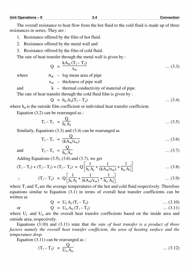
Unit Operations – II 3.4 Convection
The overall resistance to heat flow from the hot fluid to the cold fluid is made up of three
resistances in series. They are :
1. Resistance offered by the film of hot fluid.
2. Resistance offered by the metal wall and
3. Resistance offered by the film of cold fluid.
The rate of heat transfer through the metal wall is given by :
Q = kAw (T2 – T3)
xw … (3.3)
where Aw – log mean area of pipe
xw – thickness of pipe wall
and k – thermal conductivity of material of pipe.
The rate of heat transfer through the cold fluid film is given by :
Q = ho Ao(T3 – T4) … (3.4)
where ho is the outside film coefficient or individual heat transfer coefficient.
Equation (3.2) can be rearranged as :
T1 – T2 = Q
hi Ai … (3.5)
Similarly, Equations (3.3) and (3.4) can be rearranged as
T2 – T3 = Q
(kAw/xw) … (3.6)
and T3 – T4 = Q
ho Ao … (3.7)
Adding Equations (3.5), (3.6) and (3.7), we get
(T1 – T2) + (T2 – T3) + (T3 – T4) = Q
1
hi Ai +
1
(kAw/xw) +
1
ho Ao … (3.8)
∴ (T1 – T4) = Q
1
hi Ai +
1
(kAw/xw) +
1
ho Ao … (3.9)
where T1 and T4 are the average temperatures of the hot and cold fluid respectively. Therefore
equations similar to Equation (3.1) in terms of overall heat transfer coefficients can be
written as
Q = Ui Ai (T1 – T4) … (3.10)
or Q = Uo Ao (T1 – T4) … (3.11)
where Ui and Uo are the overall heat transfer coefficients based on the inside area and
outside area, respectively.
Equations (3.10) and (3.11) state that the rate of heat transfer is a product of three
factors namely the overall heat transfer coefficient, the area of heating surface and the
temperature drop.
Equation (3.11) can be rearranged as :
(T1 – T4) = Q
Uo Ao … (3.12)
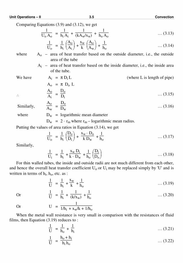
Unit Operations – II 3.5 Convection
Comparing Equations (3.9) and (3.12), we get
1
Uo Ao =
1
hi Ai +
1
(kAw/xw) +
1
ho Ao … (3.13)
1
Uo =
1
hi
Ao
Ai +
xw
k
Ao
Aw +
1
ho … (3.14)
where Ao – area of heat transfer based on the outside diameter, i.e., the outside
area of the tube
Ai – area of heat transfer based on the inside diameter, i.e., the inside area
of the tube.
We have Ai = π Di L (where L is length of pipe)
Ao = π Do L
∴
Ao
Ai =
Do
Di … (3.15)
Similarly, Ao
Aw =
Do
Dw … (3.16)
where Dw = logarithmic mean diameter
Dw = 2 · rm where rm – logarithmic mean radius.
Putting the values of area ratios in Equation (3.14), we get
1
Uo =
1
hi
Do
Di +
xw · Do
k Dw +
1
ho … (3.17)
Similarly,
1
Ui =
1
hi +
xw Di
k · Dw +
1
ho
Di
Do … (3.18)
For thin walled tubes, the inside and outside radii are not much different from each other,
and hence the overall heat transfer coefficient Uo or Ui may be replaced simply by 'U' and is
written in terms of hi, ho, etc. as :
1
U =
1
hi +
xw
k +
1
ho … (3.19)
Or 1
U =
1
hi +
1
(k/xw) +
1
ho … (3.20)
Or U = 1
1/hi + xw/k + 1/ho
When the metal wall resistance is very small in comparison with the resistances of fluid
films, then Equation (3.19) reduces to :
1
U =
1
ho +
1
hi … (3.21)
1
U =
ho + hi
hi ho … (3.22)
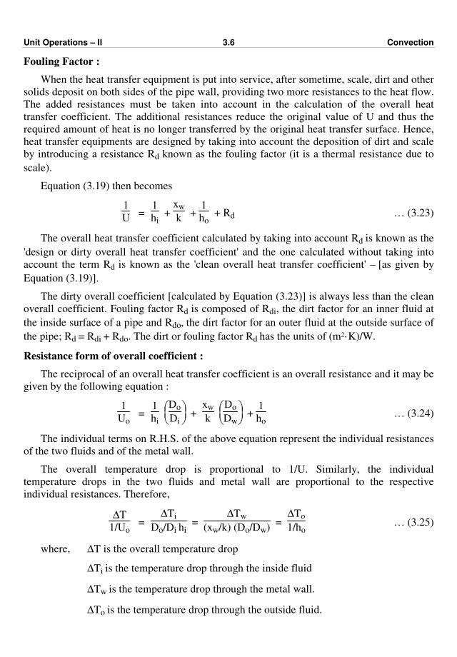
Unit Operations – II 3.6 Convection
Fouling Factor :
When the heat transfer equipment is put into service, after sometime, scale, dirt and other
solids deposit on both sides of the pipe wall, providing two more resistances to the heat flow.
The added resistances must be taken into account in the calculation of the overall heat
transfer coefficient. The additional resistances reduce the original value of U and thus the
required amount of heat is no longer transferred by the original heat transfer surface. Hence,
heat transfer equipments are designed by taking into account the deposition of dirt and scale
by introducing a resistance Rd known as the fouling factor (it is a thermal resistance due to
scale).
Equation (3.19) then becomes
1
U =
1
hi +
xw
k +
1
ho + Rd … (3.23)
The overall heat transfer coefficient calculated by taking into account Rd is known as the
'design or dirty overall heat transfer coefficient' and the one calculated without taking into
account the term Rd is known as the 'clean overall heat transfer coefficient' – [as given by
Equation (3.19)].
The dirty overall coefficient [calculated by Equation (3.23)] is always less than the clean
overall coefficient. Fouling factor Rd is composed of Rdi, the dirt factor for an inner fluid at
the inside surface of a pipe and Rdo, the dirt factor for an outer fluid at the outside surface of
the pipe; Rd = Rdi + Rdo. The dirt or fouling factor Rd has the units of (m2·K)/W.
Resistance form of overall coefficient :
The reciprocal of an overall heat transfer coefficient is an overall resistance and it may be
given by the following equation :
1
Uo =
1
hi
Do
Di +
xw
k
Do
Dw +
1
ho … (3.24)
The individual terms on R.H.S. of the above equation represent the individual resistances
of the two fluids and of the metal wall.
The overall temperature drop is proportional to 1/U. Similarly, the individual
temperature drops in the two fluids and metal wall are proportional to the respective
individual resistances. Therefore,
∆T
1/Uo =
∆Ti
Do/Di hi =
∆Tw
(xw/k) (Do/Dw) =
∆To
1/ho … (3.25)
where, ∆T is the overall temperature drop
∆Ti is the temperature drop through the inside fluid
∆Tw is the temperature drop through the metal wall.
∆To is the temperature drop through the outside fluid.

Unit Operations – II 3.7 Convection
Magnitude of film heat transfer coefficients :
Table 3.1 gives the range of values of the film heat transfer coefficients for various
processes of heat transfer.
Table 3.1 : Magnitudes of film heat transfer coefficients (hi or ho)
Type of Processes Range of values of h in
W/(m2·K)
No phase change :
Water (heating or cooling)
Gases (heating or cooling)
Air (heating or cooling)
Oils (heating or cooling)
Organic solvents (heating or cooling)
Condensing :
Condensing steam (film-type condensation)
Condensing organic vapours
Ammonia
Condensing steam (drop-wise condensation)
Evaporation :
Water
Organic solvents
Ammonia
300 – 20,000
20 – 300
1 – 50
50 – 1500
350 – 3000
6000 – 20,000
1000 – 2000
3000 – 6000
30,000 – 100,000
2000 – 12000
600 – 2000
1100 – 2300
Table 3.2 gives the range of values of the overall heat transfer coefficients for various
fluid systems in a shell and tube equipment.
Table 3.2 : Approximate range of values of overall heat transfer coefficients, U
Hot side (Hot fluid) Cold side
(Cold fluid)
Overall U in
W/(m2·K)
Heat exchangers (without phase change) :
Water
Gases
Organic solvents
Water
Gases
Heavy organics
Water
Water
Water
Brine
Brine
Heavy organics
900 – 1700
20 – 300
300 – 900
600 – 1200
20 – 300
50 – 300
Heaters :
Steam
Steam
Dowtherm
Steam
Steam
Water
Gases
Gases
Light oils
Organic solvents
1500 – 4000
30 – 300
20 – 200
300 – 900
600 – 1200
… Contd.

Unit Operations – II 3.8 Convection
Evaporators : Steam
Steam
Steam
Water
Water
Organic solvents
Light oils
Refrigerants
2000 – 4000
600 – 1200
400 – 1000
400 – 900
Condensers : Steam
Saturated organic solvents
Low boiling hydrocarbons
Organic solvents with high noncondensable
Water
Water
Water
Water
2000 – 4000
600 – 1200
400 – 1200
100 – 500
Classification of individual heat transfer coefficients :
The problem of predicting the rate of heat transfer from one fluid to another through a
metal wall reduces essentially to the problem of predicting the values of the film coefficients
of the fluids involved in the overall process. In practice, we come across a variety of cases
and each one must be considered separately. The cases that come across in practice may be
classified as
(a) Heat transfer to or from fluids inside tubes, without phase change.
(b) Heat transfer to or from fluids outside tubes, without phase change.
(c) Heat transfer from condensing vapours.
(d) Heat transfer to boiling liquids.
Sensible heat :
It is the heat that must be transferred either to raise or lower the temperature of a
substance or mixture of substances. It is the heat added or removed from a system to increase
or decrease the temperature of the system without changing its phase. The sensible heat
transfer is given by
Q = m Cp ∆T or ⋅m Cp ∆T
Latent heat :
When a matter undergoes a phase change, the enthalpy change associated with unit
amount of matter at constant temperature and pressure is known as the latent heat of phase
change. The latent heat transfer is given by Q = mλ or ⋅mλ where m is the mass and
⋅m is the
mass flow rate.
Heat transfer to fluids without phase change : In most of the heat exchange
applications, heat is transferred between fluid streams without a phase change in the fluids.
Examples of this type of heat transfer are :
Heat exchange between hot and cooler petroleum streams.
Heat transfer from a stream of hot gas to cooling water.
Cooling of a hot liquid stream by cooling water/air.
In such cases the two streams are separated by a metal wall that constitutes the heat
transfer surface. The surface may consist of tubes, or other channels of constant cross section
or of flat plates.
A fluid being heated or cooled may be flowing in laminar flow, in turbulent flow or in
the transition range between laminar and turbulent.

Unit Operations – II 3.9 Convection
An equation for predicting the film coefficient or the surface coefficient in any particular
case must include all the properties of the fluid and conditions of its flow that affect the
problem. In a particular case the factors that might be considered are the diameter of pipe,
the velocity of flowing fluid, density, viscosity, thermal conductivity, specific heat of the
fluid, etc. The dimensional analysis is one of the most useful methods to assemble these
variables/factors into an equation. This method results in arranging the variables into various
dimensionless groups.
It is found that an equation for the film coefficient for heat transfer to or from a flowing
fluid without phase change will probably be of the form :
NNu = f
NRe‚ NPr‚ NGr ‚ L
D
Application of Dimensional Analysis to heat transfer by convection :
Dimensional analysis is a method of correlating a number of variables into a single
equation that clearly states an effect. When the value of a given particular physical quantity is
influenced by a number of variables, then it is impossible to determine their individual
effects by the experimental methods. In such cases, a problem can be more easily handled by
using the method of dimensional analysis wherein the variables are arranged in
dimensionless groups which are significantly less than the number of variables. Dimensional
analysis finds application in many areas of chemical engineering such as fluid flow, heat
transfer, etc.
The rate of heat transfer per unit area depends on the viscosity µ, density ρ, specific heat
capacity Cp, thermal conductivity of the fluid k, a linear dimension of the surface l, the
velocity of the flowing fluid u, the temperature difference, ∆T, and the product of the thermal
expansion coefficient, β and the acceleration due to gravity, g. The relationship between the
heat flux and the above cited parameters may be given as
Q
A = α [ua lb ρc C
d
p ∆Te (β·g)f ki, µm] … (3.26)
The dimensions of the variables in terms of length L, mass M, time θ, temperature T, and
heat H are given as follows :
Q/A rate of heat transfer per unit area H L–2 θ–1
u velocity of the flowing fluid L θ–1
l linear dimension of the surface L
µ viscosity of the flowing fluid M L–1 θ–1
ρ density of the flowing fluid M L–3
k thermal conductivity of the flowing fluid H L–1 θ–1 T–1
Cp specific heat of the flowing fluid H M–1 T–1
∆T temperature difference T
(β · g) coefficient of thermal expansion times T–1 L θ–2
the acceleration due to gravity.

Unit Operations – II 3.10 Convection
Substituting the dimensions of each term in Equation (3.26) gives
(HL–2 θ–1) = α (Lθ–1)a (L)b (ML–3)c (HM–1 T–1)d (T)e (T–1 Lθ–2)f ×
× (HL–1 θ–1 T–1)i × (ML–1 θ–1)m … (3.27)
Equating the indices of the dimensions L, θ, H, etc. on LHS with those on RHS of
Equation (3.27), we get
in length – 2 = a + b – 3c + f – i – m
in mass 0 = c – d + m
in time – 1 = – a – 2f – i – m
in temperature 0 = – d + e – f – i
in heat 1 = d + i
There are five equations (in length, mass, time, temperature and heat) and nine variables
so that the above equation (i.e., Equation 3.27) will be rearranged in four dimensionless
groups in terms of any three indices. Let us choose a, f and d be the three indices.
Let us obtain the other constants in terms of a, f and d.
We have 1 = d + i
∴ i = 1 – d
We have – 1 = – a – 2f – i – m
∴ – 1 = – a – 2f – (1 – d) – m
∴ m = d – a – 2f
We have 0 = – d + e – f – i
0 = – d + e – f – (1 – d)
∴ e = 1 + f
0 = c – d + m
0 = c – d + d – a – 2f
∴ c = a + 2f
– 2 = a + b – 3c + f – i – m
– 2 = a + b – 3 (a + 2f) + f – (1 – d) – (d – a – 2f)
∴ b = – 1 + a + 3f
Substituting for b, c, e, i and m, Equation (3.27) becomes
Q
A = α [(u)a (l)–1 + a1 + 3f (ρ) a+2f (Cp)d (∆T)1+f × (βg)f (k)1–d (µ)d – a – 2f] … (3.28)
Collecting the terms, we get
Q
A = α
k ∆T
l
l uρ
µ
a
Cp µ
k
d
βg ∆T l3 ρ2
µ2
f … (3.29)
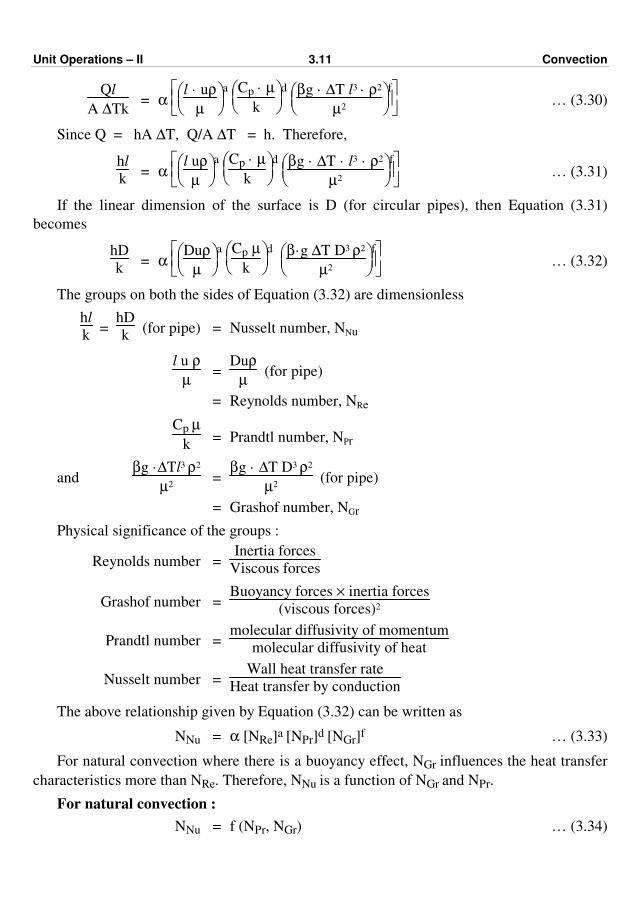
Unit Operations – II 3.11 Convection
Ql
A ∆Tk = α
l · uρ
µ
a
Cp · µ
k
d
βg · ∆T l3 · ρ2
µ2
f … (3.30)
Since Q = hA ∆T, Q/A ∆T = h. Therefore,
hl
k = α
l uρ
µ
a
Cp · µ
k
d
βg · ∆T · l3 · ρ2
µ2
f … (3.31)
If the linear dimension of the surface is D (for circular pipes), then Equation (3.31)
becomes
hD
k = α
Duρ
µ
a
Cp µ
k
d
β·g ∆T D3 ρ2
µ2
f … (3.32)
The groups on both the sides of Equation (3.32) are dimensionless
hl
k =
hD
k (for pipe) = Nusselt number, NNu
l u ρ
µ =
Duρ
µ (for pipe)
= Reynolds number, NRe
Cp µ
k = Prandtl number, NPr
and βg ·∆Tl3 ρ2
µ2 =
βg · ∆T D3 ρ2
µ2 (for pipe)
= Grashof number, NGr
Physical significance of the groups :
Reynolds number = Inertia forces
Viscous forces
Grashof number = Buoyancy forces × inertia forces
(viscous forces)2
Prandtl number = molecular diffusivity of momentum
molecular diffusivity of heat
Nusselt number = Wall heat transfer rate
Heat transfer by conduction
The above relationship given by Equation (3.32) can be written as
NNu = α [NRe]a [NPr]d [NGr]f … (3.33)
For natural convection where there is a buoyancy effect, NGr influences the heat transfer
characteristics more than NRe. Therefore, NNu is a function of NGr and NPr.
For natural convection :
NNu = f (NPr, NGr) … (3.34)

Unit Operations – II 3.12 Convection
For forced convection, Reynold's number influences the heat transfer characteristics and
the Grashof number may be omitted. Therefore, for forced convection, we have
NNu = f (NRe, NPr) … (3.35 a)
I. Application of dimensional analysis for a forced convection equation :
To derive a relationship for heat transfer coefficient, h for forced convection heat transfer
on the assumption that the coefficient h is a function of the following variables :
l – linear dimension of the surface
Cp – specific heat of the fluid
ρ – density of the fluid
µ – viscosity of the fluid
k – thermal conductivity of the fluid
and u – velocity of the fluid.
Solution : It is given that h is a function of L, u, ρ, µ, Cp and k. Therefore, we can
write
h = f (ρ, u, L, µ, Cp, k)
h = A (ρa ub Lc µd Ce
p kf) … (3.35 b)
where A, a, b, c, d, e, and f are constants.
Express the energy terms mechanically by dimensions of the variables :
The dimensions of each variable in terms of M, L, T, θ and F are :
Parameter Units Fundamental dimensions
h
k
Cp
µ
u
l
ρ
N.m/(m2·s·K) = W/(m2·K)
N·m/(m·s·K) = W/(m·K)
N·m/(kg·K) = J/(kg·K)
kg/(m·s)
m/s
m
kg/m3
FL/L2θT = FL–1 θ–1 T–1
FL/LθT = Fθ–1 T–1
FL/MT = FLM–1 T–1
M/Lθ = ML–1 θ–1
L/θ = Lθ–1
L = L
M/L3 = ML–3
Substituting the dimensions of all parameters in the above equation, we get
FL–1 θ–1 T–1 = A (ML–3)a (Lθ–1)b (L)c (ML–1 θ–1)d (FLM–1 T–1)e (Fθ–1 T–1)f … (1)
Equating the indices/powers of M, L, θ, T and F, on LHS with those on RHS of the above
equation gives
Force, F : 1 = e + f … (i)
Mass, M : 0 = a + d – e … (ii)
Length, L : – 1 = – 3a + b + c – d + e … (iii)
Temperature, T : – 1 = – e – f … (iv)
Time, θ : – 1 = – b – d – f … (v)
Let us obtain the constants c, d, etc. in terms of a and e.
Unit Operations – II 3.13 Convection
From Equation (i),
f = 1 – e
From Equation (ii),
d = e – a
From Equation (v),
– 1 = – b – d – f
b = 1 – d – f = 1 – (e – a) – f
b = 1 – e + a – f
b = a + (1 – e) – f = a + f – f
∴ b = a
From Equation (iii),
– 1 = – 3a + b + c – d + e
c = 3a – b + d – e – 1
= 3a – a + (e – a) – e – 1
c = 2a – a – 1 = a – 1
Substituting back, Equation (1) becomes
h = A (ρ)a (u)a (L)a–1 (µ)e–a (Cp)e (k)1–e
Collecting the terms, we get
h = A
Luρ
µ
a
Cp µ
k
e
(k/L)
∴ hL
k = A
Luρ
µ
a
Cp µ
k
e
… (3.35 c)
In the case of pipe, the linear dimension is D (inside diameter) and the above equation
becomes
hD
k = A
Duρ
µ
a
Cp µ
k
e
We can obtain the same expression if we express energy terms thermally by the
dimensions of the variables.
Equation (3.35 c) is the required relationship; where A, a and e must be evaluated from a
minimum of three sets of experimental data.
This equation contains three dimensionless groups/numbers :
(i) Nusselt number, NNu = hL/k

Unit Operations – II 3.14 Convection
(ii) Reynolds number, NRe = Luρ/µ
(iii) Prandtl number, NPr = Cp µ/k.
Let us obtain the same relationship by expressing energy terms thermally.
Expressing the energy terms thermally by dimensions of the variables :
Parameter Units Fundamental dimensions
h
k
Cp
µ
u
l
ρ
W/(m2·K) = J/(s·m2·K)
W/(m·K) = J/(s·m·K)
J/(kg·K)
kg/(m·s)
m/s
m
kg/m3
H/θL2T = Hθ–1 L–2 T–1
H/θLT = H θ–1 L–1 T–1
H/MT = HM–1 T–1
M/Lθ = ML–1 θ–1
L/θ = Lθ–1
L = L
M/L3 = ML–3
Substituting the dimensions of all the parameters, we get
Hθ–1 L–2 T–1 = A (ML–3)a (Lθ–1)b (L)c (ML–1 θ–1)d (HM–1 T–1)e (Hθ–1 L–1 T–1)f
Equating the indices/powers of M, L, θ, etc. on LHS and RHS of the above equation
gives
H : 1 = e + f … (i)
M : 0 = a + d – e … (ii)
L : – 2 = – 3a + b + c – d – f … (iii)
θ : – 1 = – b – d – f … (iv)
T : – 1 = – e – f … (v)
Let us obtain indices f, d, etc. in terms of a and e.
From equation (i), f = 1 – e
From equation (ii), d = e – a
From equation (iv), b = 1 – d – f = 1 – e + a – 1 + e = a
From equation (iii), c = a – 1
Substituting back values of the indices b, c, d and f in Equation (3.35 b),
h = A (ρ)a (u)a (L)a–1 (µ)e–a (Cp)e (k)1–e
Collecting the terms, we get
h = A
Luρ
µ
a (Cpµ/k)e (k/L)
∴ hL
k = A
Luρ
µ
a (Cpµ/k)e … (3.35 d)
II. Application of dimensional analysis for a natural convection equation :
To derive a relationship for the heat transfer coefficient h for natural convection between
a surface and a fluid assuming that the coefficient h is a function of the following variables :
l – a characteristic linear dimension of the surface,
ρ – density of the fluid,
µ – viscosity of the fluid,
k – thermal conductivity of the fluid,
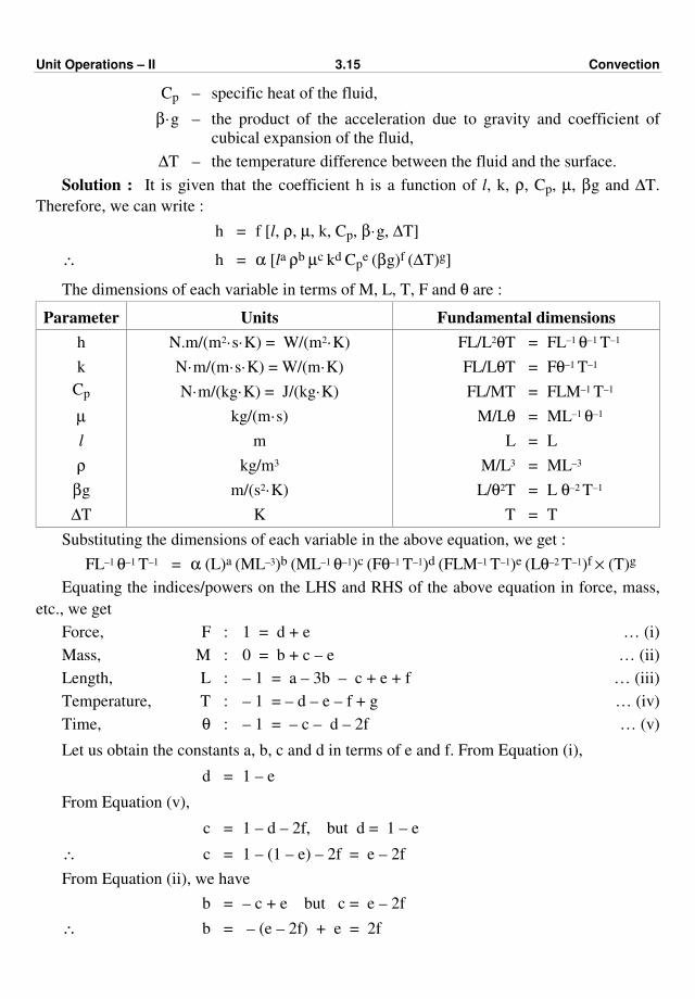
Unit Operations – II 3.15 Convection
Cp – specific heat of the fluid,
β·g – the product of the acceleration due to gravity and coefficient of
cubical expansion of the fluid,
∆T – the temperature difference between the fluid and the surface.
Solution : It is given that the coefficient h is a function of l, k, ρ, Cp, µ, βg and ∆T.
Therefore, we can write :
h = f [l, ρ, µ, k, Cp, β·g, ∆T]
∴ h = α [la ρb µc kd Cpe (βg)f (∆T)g]
The dimensions of each variable in terms of M, L, T, F and θ are :
Parameter Units Fundamental dimensions
h
k
Cp
µ
l
ρ
βg
∆T
N.m/(m2·s·K) = W/(m2·K)
N·m/(m·s·K) = W/(m·K)
N·m/(kg·K) = J/(kg·K)
kg/(m·s)
m
kg/m3
m/(s2·K)
K
FL/L2θT = FL–1 θ–1 T–1
FL/LθT = Fθ–1 T–1
FL/MT = FLM–1 T–1
M/Lθ = ML–1 θ–1
L = L
M/L3 = ML–3
L/θ2T = L θ–2 T–1
T = T
Substituting the dimensions of each variable in the above equation, we get :
FL–1 θ–1 T–1 = α (L)a (ML–3)b (ML–1 θ–1)c (Fθ–1 T–1)d (FLM–1 T–1)e (Lθ–2 T–1)f × (T)g
Equating the indices/powers on the LHS and RHS of the above equation in force, mass,
etc., we get
Force, F : 1 = d + e … (i)
Mass, M : 0 = b + c – e … (ii)
Length, L : – 1 = a – 3b – c + e + f … (iii)
Temperature, T : – 1 = – d – e – f + g … (iv)
Time, θ : – 1 = – c – d – 2f … (v)
Let us obtain the constants a, b, c and d in terms of e and f. From Equation (i),
d = 1 – e
From Equation (v),
c = 1 – d – 2f, but d = 1 – e
∴ c = 1 – (1 – e) – 2f = e – 2f
From Equation (ii), we have
b = – c + e but c = e – 2f
∴ b = – (e – 2f) + e = 2f

Unit Operations – II 3.16 Convection
From Equation (iii), we have
a = – 1 + 3b + c – e – f
a = – 1 + 3 (2f) + (e – 2f) – e – f = – 1 + 3f
From Equation (iv), we have
g = – 1 + d + e + f = – 1 + 1 + f = f [as d + e = 1]
Substituting back the values of constants a, b, c and d, the equation for h becomes
h = α (l)–1 + 3f (ρ)2f (µ)e–2f (k)1–e (Cp)e (βg)f (∆T)f
Collecting the terms, we get
h = α
Cpµ
k
e
l3 ρ2 βg ∆T
µ2
f
(k/L)
∴ hL
k = α
Cp µ
k
e
l3 ρ2 βg ∆T
µ2
f
… (3.35 e)
Equation (3.35 e) is the desired relationship for natural convection.
Here Cp µ
k is the Prandtl number (NPr)
hL/k is the Nusselt number (NNu)
and l3 ρ2 β·g ∆T
µ2 is the Grashof number (Nar)
Empirical equations for calculation of heat transfer coefficients in laminar, turbulent
and transition region in forced convection :
[A] Film coefficients-in pipes – Laminar flow :
Heat transfer to laminar flow may be occurred whenever fluids to be heated or cooled are
viscous or flow rates are low. In polymer, food or pharmaceutical industry, we may come
across a heat exchanger where the flow is in the laminar region (NRe < 2100).
For heating or cooling of viscous fluids, an empirical correlation is
NNu = 1.86 [(NRe) (NPr) (D/L)]1/3 [µ/µw]0.14 … (3.36)
Equation (3.36) is the Sider-Tate equation for the calculation of the heat transfer
coefficient for laminar flow of fluids in horizontal tubes or pipes. Equation (3.36) is valid for
NRe < 2100 and (NRe NPr , D/L) > 100
where D is the diameter of pipe and L is the length of pipe.
The term (µ/µw)0.14 is called as the Sider-Tate correction. The term (µ/µw) is the ratio of
the viscosity of the fluid at the bulk temperature and the viscosity of the fluid at the wall
temperature.
hD
k = 1.86
Duρ
µ
Cp µ
k D
L
1/3
µ
µw
0.14
… (3.37)
where h is the inside heat transfer coefficient, D is the inside diameter of pipe.
Unit Operations – II 3.17 Convection
In the above equation all the physical properties of the fluid are taken at the mean bulk
temperature of the flowing fluid, i.e., at the arithmetic mean of inlet and outlet temperatures
of the fluid flowing through pipe (Ti + To)/2 and µw is evaluated at the average wall
temperature.
Graetz number is defined by the following equation
NGz =
.m Cp
kL … (3.38)
where .
m is the mass flow rate
.
m = ρuA = π4
ρuD2 … (3.39)
NGz = π4
ρu Cp D2
k L
= π4
Duρ
µ
Cp µ
k ·
D
L
= π4
NRe · NPr · D
L … (3.40)
By substituting for NRe · NPr · D
L from Equation (3.40), Equation (3.36) becomes :
NNu = 1.86
4
π (NGz)
1/3
×
µ
µw
0.14
NNu = 2 [NGz]1/3 [µ/µw]0.14 … (3.41)
hD
k = 2.0
.
m Cp
k L
1/3
[µ/µw]0.14 … (3.42)
Equation (3.42) is the Sider-Tate equation for laminar flow/viscous flow in terms of the
Graetz number.
The Peclet number is defined as the product of the Reynolds number and Prandtl number.
NPe = NRe · NPr = Duρ
µ ·
Cp µ
k =
Du
α … (3.43)
α = k/ρCp, α is the thermal diffusivity and has units of m2/s.
The choice among these groups is arbitrary.
For thin fluids in laminar flow :
For values of (NRe · NPr D/L) > 12, the following empirical equation is applicable :
NNu = 1.62
NRe · NPr · D
L
1/3
… (3.44)
Equation (3.44) can be written as
NNu = 1.75
.
m Cp
k L
1/3
… (3.45)
For viscous liquids in laminar flow, Equation (3.42) is applicable in which variation of
viscosity with temperature is introduced.
Unit Operations – II 3.18 Convection
[B] Film coefficients - in pipes – Turbulent flow :
The most important situation in heat transfer is the flow of heat in a stream of fluid in
turbulent flow in pipes or tubes. Turbulence is encountered at NRe > 2100. As the rate of heat
transfer is greater in turbulent flow than in laminar flow, most of the heat transfer equipments
are operated in the turbulent range.
The Dittus-Boelter equation for predicting the heat transfer coefficient for turbulent flow
in tubes or pipes is
hD
k = 0.023
Duρ
µ
0.8
Cp µ
k
a
… (3.46)
where 'a' has a value of 0.4 for heating and 0.3 for cooling. It is commonly used for water like
materials.
Here also the fluid properties are evaluated at the arithmetic mean bulk temperature,
i.e., at (Ti + To)/2 of the flowing fluid. Ti and To are the inlet and outlet temperatures.
For heating :
NNu = 0.023 [NRe]0.8 [NPr]0.4 … (3.47)
For cooling :
NNu = 0.023 [NRe]0.8 [NPr]0.3 … (3.48)
Equations (3.47) and (3.48) are valid for Reynolds number greater than 10000 and
Prandtl number between 0.7 and 160.
For turbulent flow in tubes/pipes, the Sieder-Tate equation that takes into account the
variation of the viscosity of the fluid near the wall with thermal gradients is
hD
k = 0.023
Duρ
µ
0.8
Cp µ
k
1/3
(µ/µw)0.14 … (3.49)
Equation (3.49) is the Sieder-Tate equation.
Equation (3.49) is valid for NRe > 10,000 and 0.7 < NPr < 700 and L/D > 60. The
term (µ/µw)0.14 is called as the Sieder-Tate correction factor.
Here all the fluid properties are taken at the mean bulk temperature, i.e., at (Ti + To)/2,
where Ti is inlet fluid temperature and To is the fluid outlet temperature. µw is the viscosity of
fluid at the wall temperature.
An alternate equation that in many ways is more convenient is the one proposed by
Colburn.
In the Colburn equation, the Stanton number (Nst) is used instead of the Nusselt number
(NNu) :
Nst = h
Cp ρu … (3.50)
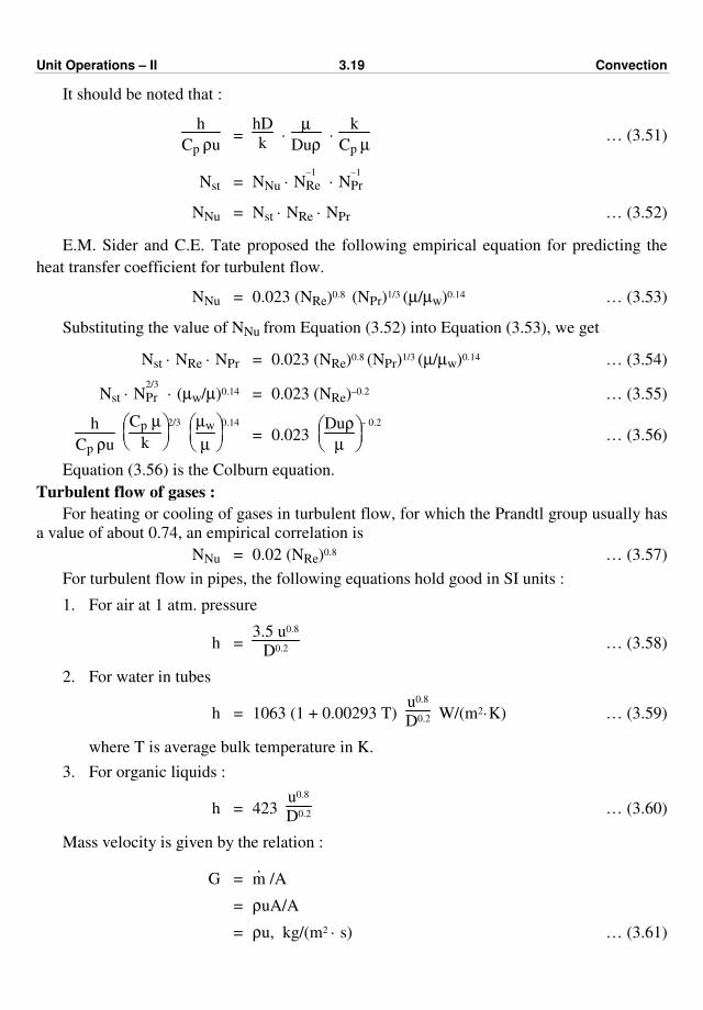
Unit Operations – II 3.19 Convection
It should be noted that :
h
Cp ρu =
hD
k ·
µ
Duρ ·
k
Cp µ … (3.51)
Nst = NNu · N–1
Re · N–1
Pr
NNu = Nst · NRe · NPr … (3.52)
E.M. Sider and C.E. Tate proposed the following empirical equation for predicting the
heat transfer coefficient for turbulent flow.
NNu = 0.023 (NRe)0.8 (NPr)1/3 (µ/µw)0.14 … (3.53)
Substituting the value of NNu from Equation (3.52) into Equation (3.53), we get
Nst · NRe · NPr = 0.023 (NRe)0.8 (NPr)1/3 (µ/µw)0.14 … (3.54)
Nst · N2/3
Pr · (µw/µ)0.14 = 0.023 (NRe)–0.2 … (3.55)
h
Cp ρu
Cp µ
k
2/3
µw
µ
0.14
= 0.023
Duρ
µ
– 0.2
… (3.56)
Equation (3.56) is the Colburn equation.
Turbulent flow of gases :
For heating or cooling of gases in turbulent flow, for which the Prandtl group usually has
a value of about 0.74, an empirical correlation is
NNu = 0.02 (NRe)0.8 … (3.57)
For turbulent flow in pipes, the following equations hold good in SI units :
1. For air at 1 atm. pressure
h = 3.5 u0.8
D0.2 … (3.58)
2. For water in tubes
h = 1063 (1 + 0.00293 T) u0.8
D0.2 W/(m2·K) … (3.59)
where T is average bulk temperature in K.
3. For organic liquids :
h = 423 u0.8
D0.2 … (3.60)
Mass velocity is given by the relation :
G = .
m /A
= ρuA/A
= ρu, kg/(m2 · s) … (3.61)
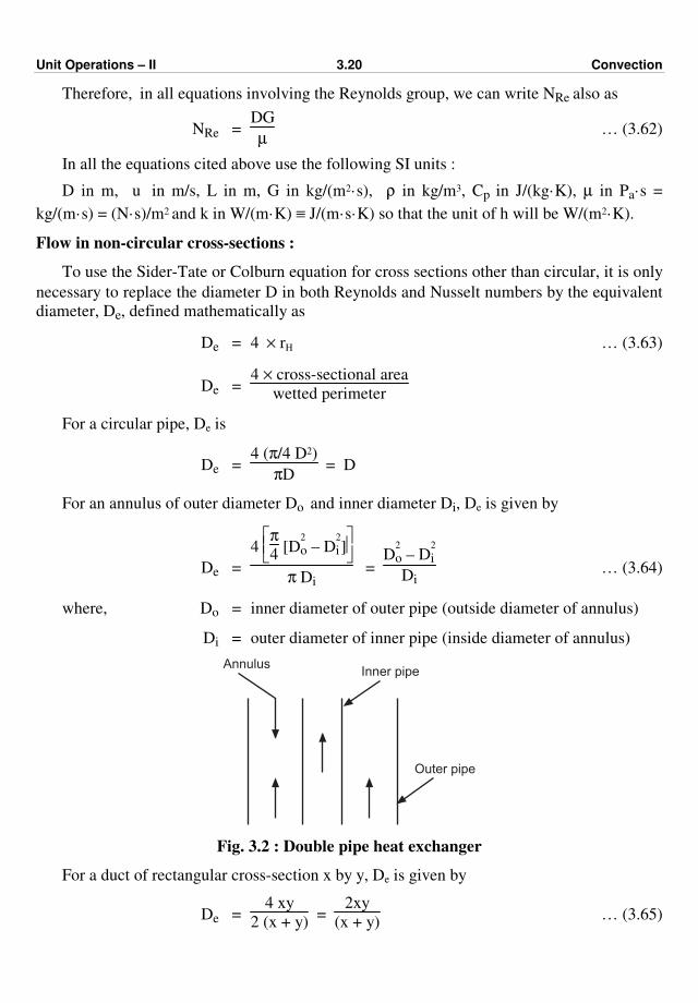
Unit Operations – II 3.20 Convection
Therefore, in all equations involving the Reynolds group, we can write NRe also as
NRe = DG
µ … (3.62)
In all the equations cited above use the following SI units :
D in m, u in m/s, L in m, G in kg/(m2·s), ρ in kg/m3, Cp in J/(kg·K), µ in Pa·s =
kg/(m·s) = (N·s)/m2 and k in W/(m·K) ≡ J/(m·s·K) so that the unit of h will be W/(m2·K).
Flow in non-circular cross-sections :
To use the Sider-Tate or Colburn equation for cross sections other than circular, it is only
necessary to replace the diameter D in both Reynolds and Nusselt numbers by the equivalent
diameter, De, defined mathematically as
De = 4 × rH … (3.63)
De = 4 × cross-sectional area
wetted perimeter
For a circular pipe, De is
De = 4 (π/4 D2)
πD = D
For an annulus of outer diameter Do and inner diameter Di, De is given by
De =
4
π
4 [D
2
o – D2
i]
π Di =
D2
o – D2
i
Di … (3.64)
where, Do = inner diameter of outer pipe (outside diameter of annulus)
Di = outer diameter of inner pipe (inside diameter of annulus)
AnnulusInner pipe
Outer pipe
Fig. 3.2 : Double pipe heat exchanger
For a duct of rectangular cross-section x by y, De is given by
De = 4 xy
2 (x + y) =
2xy
(x + y) … (3.65)

Unit Operations – II 3.21 Convection
The Colburn analogy; Colburn j factor :
For NRe between 5000 – 200000, the friction factor (f) for a smooth pipe is given by the
following empirical equation
f = 0.046
Duρ
µ
– 0.2
… (3.66)
Comparison of Equation (3.66) with Equation (3.55) for heat transfer in turbulent flow
inside a pipe/tube gives
h
Cp ρu
Cp µ
k
2/3
µw
µ
0.14
≡ jH = f
2 … (3.67)
Equation (3.67) is the Colburn analogy between heat transfer and fluid friction. The
factor jH is called the Colburn j factor. Equation (3.55) can be written in the j-factor form as
given below :
jH = 0.023 (NRe)–0.2 … (3.68)
For laminar flow region, we have
NNu = 2.0
.
m Cp
k L
1/3
µ
µw
0.14
… (3.69)
Using Equation (3.40), Equation (3.69) becomes
NNu = 2.0
π
4
D
L NRe · NPr
1/3
[µ/µw]0.14 … (3.70)
Multiplying Equation (3.70) by (1/NRe) (1/NPr), we get
h
Cp ρu
Cp µ
k
2/3
µw
µ
0.14
= jH = 1.86 D
L
1/3
Duρ
µ
– 2/3
… (3.71)
[C] Film coefficients-in pipes - in Transition Region :
Equation (3.37) is valid for Reynolds numbers less than 2100 and turbulent flow
equation for predicting the heat transfer coefficient, i.e., Equation (3.55) is valid for
Reynolds numbers more than 10,000. The range of Reynolds numbers between 2100 and
10000 is called the transition region. For this, no simple equation is applicable and therefore
to obtain h, a graphical method is used. In the graphical method the Colburn j factor is
plotted against NRe at several values of L/D - with L/D as a parameter.
Equation (3.71) shows that for each value of L/D, a logarithmic plot of L.H.S.,
i.e., jH v/s NRe gives a straight line with a slope equal to (– 2/3). The lines terminate at
NRe = 2100.
Equation (3.66) when plotted on the same coordinates gives a straight line with a slope
equal to (– 0.20) for NRe > 10,000.
The transition region is represented by curved lines for NRe between 2100 and 10000.

Unit Operations – II 3.22 Convection
Fig. 3.3 covers NRe between 10000 and 30000, so Fig. 3.3 is referred in this range.
(For NRe < 1000 and NRe > 30000), Equations (3.37) and (3.55), respectively can be
used.
For the transition region, i.e., for 2100 < NRe < 10000, the following empirical equation
can be used to calculate the film heat transfer coefficient.
NNu = 0.116 [(NRe)2/3 – 125] [NPr]1/3
1 + D
L
2/3
[µ/µw]0.14 … (3.72)
0.01
m mw(
)0.1
4C
kpm
(
)2/3
h
Gi
Cp
(
)J
=H
0.001
103
N = DG/Re m 104
L/D = 50
L/D = 100
Fig. 3.3 : Tube side heat transfer curves transition range
First of all NRe is evaluated from the data provided and then from Fig. 3.3, jH is obtained
for the corresponding NRe and L/D and in turn, it gives the value of the tube side heat transfer
coefficient.
Wilson Plot :
This plot is used to determine the film heat transfer coefficients.
Consider a shell and tube heat exchanger wherein steam is condensing on the shell side
and a cold fluid is flowing through the tubes in the turbulent flow region. The overall heat
transfer coefficient is determined by the direct measurements of heat transfer rate, overall
temperature difference and area at various cold fluid velocities. In this case, the condensing
steam side coefficient (ho) remains almost constant and the resistance offered by the metal
wall is also constant. Assuming clean tubes, Equation (3.19) reduces to
1
U =
1
hi + C … (3.73)
where 'C' is a constant.
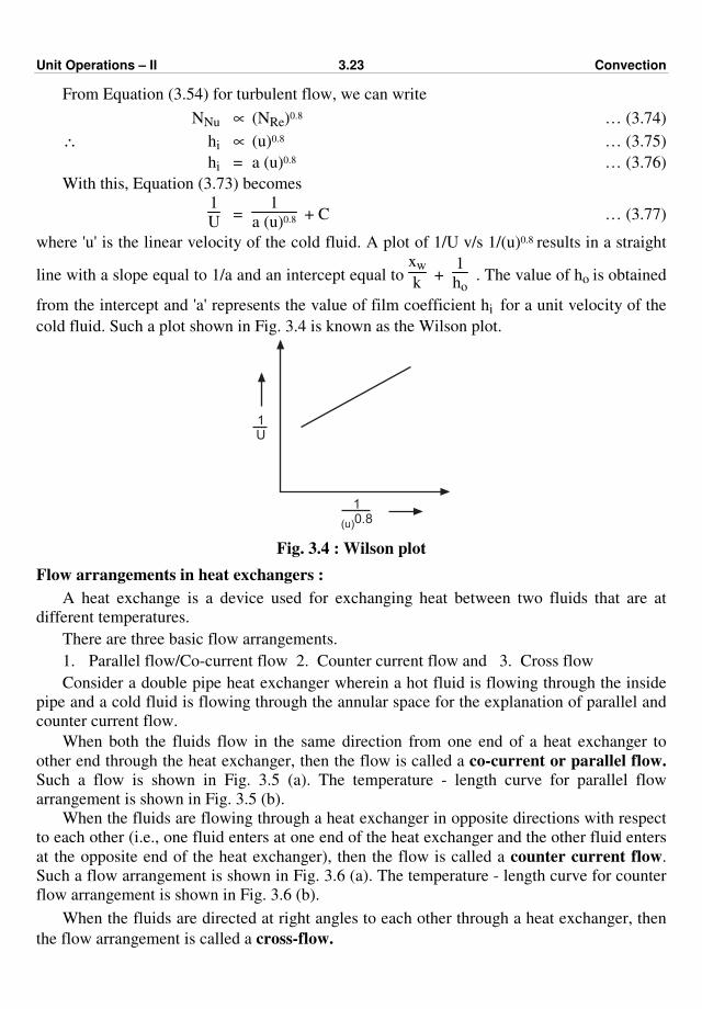
Unit Operations – II 3.23 Convection
From Equation (3.54) for turbulent flow, we can write
NNu ∝ (NRe)0.8 … (3.74)
∴ hi ∝ (u)0.8 … (3.75)
hi = a (u)0.8 … (3.76)
With this, Equation (3.73) becomes
1
U =
1
a (u)0.8 + C … (3.77)
where 'u' is the linear velocity of the cold fluid. A plot of 1/U v/s 1/(u)0.8 results in a straight
line with a slope equal to 1/a and an intercept equal to xw
k +
1
ho . The value of ho is obtained
from the intercept and 'a' represents the value of film coefficient hi for a unit velocity of the
cold fluid. Such a plot shown in Fig. 3.4 is known as the Wilson plot.
1U
10.8(u)
Fig. 3.4 : Wilson plot
Flow arrangements in heat exchangers :
A heat exchange is a device used for exchanging heat between two fluids that are at
different temperatures.
There are three basic flow arrangements.
1. Parallel flow/Co-current flow 2. Counter current flow and 3. Cross flow
Consider a double pipe heat exchanger wherein a hot fluid is flowing through the inside
pipe and a cold fluid is flowing through the annular space for the explanation of parallel and
counter current flow.
When both the fluids flow in the same direction from one end of a heat exchanger to
other end through the heat exchanger, then the flow is called a co-current or parallel flow.
Such a flow is shown in Fig. 3.5 (a). The temperature - length curve for parallel flow
arrangement is shown in Fig. 3.5 (b).
When the fluids are flowing through a heat exchanger in opposite directions with respect
to each other (i.e., one fluid enters at one end of the heat exchanger and the other fluid enters
at the opposite end of the heat exchanger), then the flow is called a counter current flow.
Such a flow arrangement is shown in Fig. 3.6 (a). The temperature - length curve for counter
flow arrangement is shown in Fig. 3.6 (b).
When the fluids are directed at right angles to each other through a heat exchanger, then
the flow arrangement is called a cross-flow.
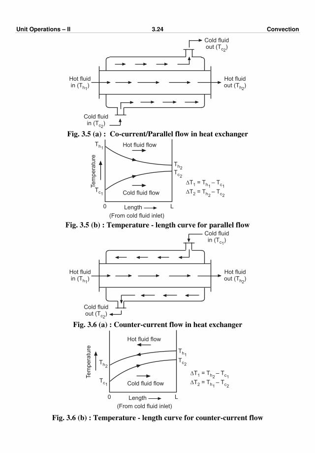
Unit Operations – II 3.24 Convection
Hot fluidin (T )h1
Cold fluidout (T )c2
Hot fluidout (T )h2
Cold fluidin (T )c2
Fig. 3.5 (a) : Co-current/Parallel flow in heat exchanger
Tem
pera
ture
Hot fluid flow
Cold fluid flow
Th1
Tc1
Th2Tc2
DT = –1 h1 c1T T
DT = –2 h2 c2T T
0 LLength
(From cold fluid inlet)
Fig. 3.5 (b) : Temperature - length curve for parallel flow
Hot fluidin (T )h1
Cold fluidin (T )c1
Hot fluidout (T )h2
Cold fluidout (T )c2
Fig. 3.6 (a) : Counter-current flow in heat exchanger
Tem
pera
ture
Hot fluid flow
Cold fluid flow
Th1
Tc1
Th2
Tc2
DT = –1 h2 c1T T
DT = –2 h1 c2T T
0 LLength
(From cold fluid inlet)
Fig. 3.6 (b) : Temperature - length curve for counter-current flow
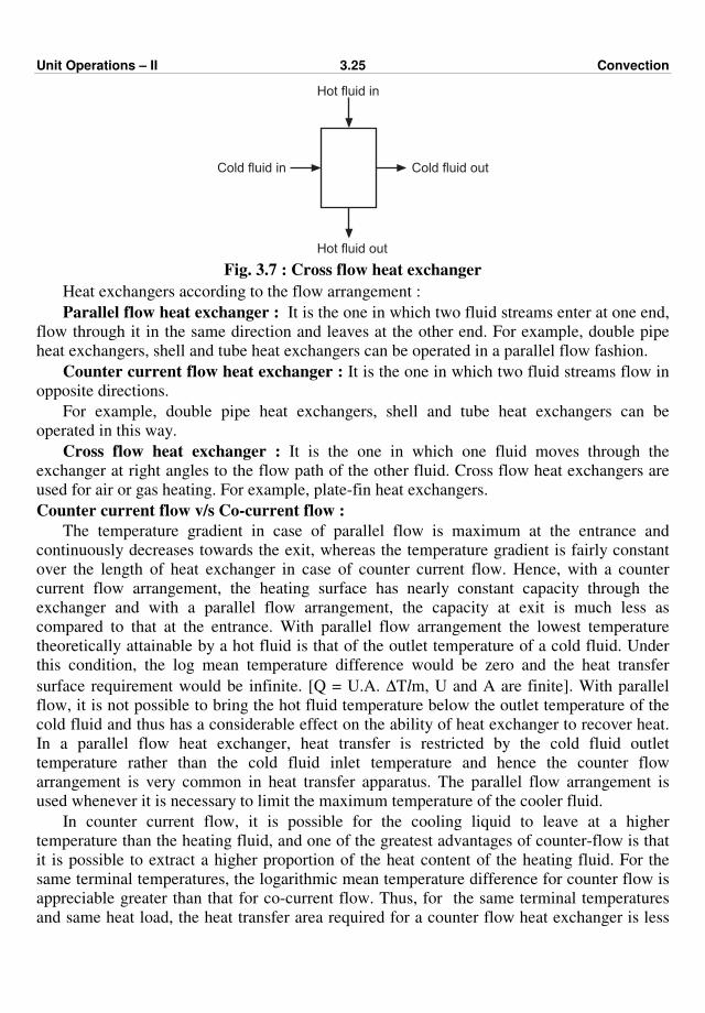
Unit Operations – II 3.25 Convection
Cold fluid in Cold fluid out
Hot fluid in
Hot fluid out
Fig. 3.7 : Cross flow heat exchanger
Heat exchangers according to the flow arrangement :
Parallel flow heat exchanger : It is the one in which two fluid streams enter at one end,
flow through it in the same direction and leaves at the other end. For example, double pipe
heat exchangers, shell and tube heat exchangers can be operated in a parallel flow fashion.
Counter current flow heat exchanger : It is the one in which two fluid streams flow in
opposite directions.
For example, double pipe heat exchangers, shell and tube heat exchangers can be
operated in this way.
Cross flow heat exchanger : It is the one in which one fluid moves through the
exchanger at right angles to the flow path of the other fluid. Cross flow heat exchangers are
used for air or gas heating. For example, plate-fin heat exchangers.
Counter current flow v/s Co-current flow :
The temperature gradient in case of parallel flow is maximum at the entrance and
continuously decreases towards the exit, whereas the temperature gradient is fairly constant
over the length of heat exchanger in case of counter current flow. Hence, with a counter
current flow arrangement, the heating surface has nearly constant capacity through the
exchanger and with a parallel flow arrangement, the capacity at exit is much less as
compared to that at the entrance. With parallel flow arrangement the lowest temperature
theoretically attainable by a hot fluid is that of the outlet temperature of a cold fluid. Under
this condition, the log mean temperature difference would be zero and the heat transfer
surface requirement would be infinite. [Q = U.A. ∆Tlm, U and A are finite]. With parallel
flow, it is not possible to bring the hot fluid temperature below the outlet temperature of the
cold fluid and thus has a considerable effect on the ability of heat exchanger to recover heat.
In a parallel flow heat exchanger, heat transfer is restricted by the cold fluid outlet
temperature rather than the cold fluid inlet temperature and hence the counter flow
arrangement is very common in heat transfer apparatus. The parallel flow arrangement is
used whenever it is necessary to limit the maximum temperature of the cooler fluid.
In counter current flow, it is possible for the cooling liquid to leave at a higher
temperature than the heating fluid, and one of the greatest advantages of counter-flow is that
it is possible to extract a higher proportion of the heat content of the heating fluid. For the
same terminal temperatures, the logarithmic mean temperature difference for counter flow is
appreciable greater than that for co-current flow. Thus, for the same terminal temperatures
and same heat load, the heat transfer area required for a counter flow heat exchanger is less
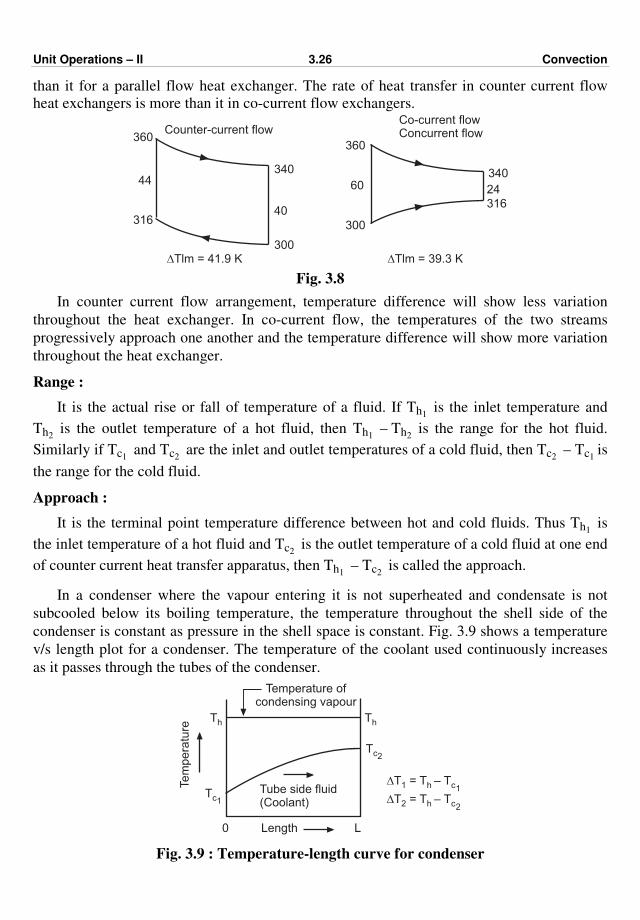
Unit Operations – II 3.26 Convection
than it for a parallel flow heat exchanger. The rate of heat transfer in counter current flow
heat exchangers is more than it in co-current flow exchangers.
360
44
31640
340
300DTlm = 41.9 K
Counter-current flow
300
360
340
316
2460
Co-current flowConcurrent flow
DTlm = 39.3 K
Fig. 3.8
In counter current flow arrangement, temperature difference will show less variation
throughout the heat exchanger. In co-current flow, the temperatures of the two streams
progressively approach one another and the temperature difference will show more variation
throughout the heat exchanger.
Range :
It is the actual rise or fall of temperature of a fluid. If Th1 is the inlet temperature and
Th2 is the outlet temperature of a hot fluid, then Th1
– Th2 is the range for the hot fluid.
Similarly if Tc1 and Tc2
are the inlet and outlet temperatures of a cold fluid, then Tc2 – Tc1 is
the range for the cold fluid.
Approach :
It is the terminal point temperature difference between hot and cold fluids. Thus Th1 is
the inlet temperature of a hot fluid and Tc2 is the outlet temperature of a cold fluid at one end
of counter current heat transfer apparatus, then Th1 – Tc2
is called the approach.
In a condenser where the vapour entering it is not superheated and condensate is not
subcooled below its boiling temperature, the temperature throughout the shell side of the
condenser is constant as pressure in the shell space is constant. Fig. 3.9 shows a temperature
v/s length plot for a condenser. The temperature of the coolant used continuously increases
as it passes through the tubes of the condenser.
Temperature ofcondensing vapour
ThTh
Tc1
Tc2
Tube side fluid(Coolant)
Length0 L
Te
mp
era
ture
DT = –1 h c1T T
DT = –2 h c2T T
Fig. 3.9 : Temperature-length curve for condenser

Unit Operations – II 3.27 Convection
Energy balances :
The energy balances are of great importance in attacking the heat transfer problems.
Consider the heat exchanger shown in Fig. 3.10.
Heat Exchanger
Cold fluid in
Hot fluid out
Cold fluid out
Hot fluid in
Fig. 3.10 : Energy balance
Let .
mc and .
mh be the mass flow rates of the cold and hot fluids respectively.
Let Hc1 and Hc2
be the enthalpies per unit mass of the cold fluid entering and leaving
the heat exchanger, respectively.
Similarly, let Hh1 and Hh2
be the enthalpies per unit mass of the hot fluid entering and
leaving the heat exchanger respectively.
Qc and Qh be the rate of heat addition to the cold fluid and hot fluid respectively. The
sign of Qh is negative since the hot fluid losses/gives out, rather than gains heat, while the
sign of Qc is positive. At steady state, the heat given out by the hot fluid is equal to the heat
gained by the cold fluid if no heat loss from the exchanger.
∴ Qc = – Qh … (3.78)
.
mc (Hc2 – Hc1 ) = –
.mh [Hh2
– Hh1 ] = Q … (3.79)
.
mc [Hc2 – Hc1 ] =
.mh [Hh2
– Hh1 ] = Q … (3.80)
If only sensible heat transfer takes place between hot and cold fluids and if constant heat
capacities are assumed, then Equation (3.80) can be written as
.
mc Cpc [Tc
2
– Tc1] =
.mh Cph
(Th1
– Th2
) = Q … (3.81)
where Cpc and Cph are the heat capacities of the cold and hot fluids respectively.
Tc1, Tc2
and Th1 and Th2
have their usual meaning. Equation (3.81) is the overall energy
or enthalpy balance over a heat exchanger equipment for sensible heat changes in both the
fluids.
For the latent heat transfer (i.e., condensation of vapours) from the condensing vapours to
a coolant, the energy balance will be :
.mh · λ =
.mc Cpc (Tc2
– Tc1) = Q … (3.82)
where .mh – rate of condensation of vapour
λ – latent heat of condensation of vapour
Equation (3.82) is applicable to a condenser where the vapour entering is saturated and
no subcooling of the condensed liquid takes place.
In the SI system, the mass flow rate is expressed usually in kg/s, the specific heat in
J/(kg·K) or kJ/(kg·K) and the rate of heat transfer in W ≡ J/s.

Unit Operations – II 3.28 Convection
Sensible Heat :
It is the heat that must be transferred to raise or lower the temperature of a substance or a
mixture of substances.
Latent Heat :
When matter undergoes a phase change (vapour to liquid, liquid to solid, etc.), the
enthalpy change associated with a unit amount of matter at constant temperature and pressure
is known as the latent heat of phase change. It is denoted by 'λ' and has the units of kJ/kg.
Heat Flux :
It is defined as the rate of heat transfer per unit area (or defined as the amount of heat
transfer per unit area per unit time). It can be based on the outside or inside heat transfer
area. It has the units of W/m2.
Log mean temperature difference :
The heat transfer flux is directly proportional to a driving force. The driving force for
heat flow is taken as Th – Tc, where Th and Tc are the temperatures of hot and cold fluids
respectively. As the term ∆T = Th – Tc varies along the length of a heat exchanger, the flux
also varies over the entire length. Consider a differential element of area dA through which a
differential amount of heat dQ flows under the driving force of ∆T. Then, dQ/dA is related to
∆T by the relation given below.
DT v/s Q
DT2
DT1
Th1
Tc2Th2
Tc1
DT1
0 Q
DT2
Tem
pera
ture
QT
Fig. 3.11 : Temperature v/s heat flow rate (counter-current flow)
dQ
dA = U · (∆T) = U · (Th – Tc) … (3.83)
where U is the local overall heat transfer coefficient, dQ/dA is the local heat flux and ∆T is
the local temperature difference.
Equation (3.83) needs to be integrated for its application to the entire area of the heat
exchanger.
Assumptions to be made for the integration of Equation (3.83) are :
1. Overall coefficient U is constant throughout the exchanger.
2. Specific heats of the hot and cold fluids are constant.
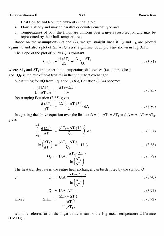
Unit Operations – II 3.29 Convection
3. Heat flow to and from the ambient is negligible.
4. Flow is steady and may be parallel or counter current type and
5. Temperatures of both the fluids are uniform over a given cross-section and may be
represented by their bulk temperatures.
Based on the assumptions (2) and (4), we get straight lines if Tc and Th are plotted
against Q and also a plot of ∆T v/s Q is a straight line. Such plots are shown in Fig. 3.11.
The slope of the plot of ∆T v/s Q is constant.
Slope = d (∆T)
dQ =
∆T2 – ∆T1
QT … (3.84)
where ∆T1 and ∆T2 are the terminal temperature differences (i.e., approaches)
and QT is the rate of heat transfer in the entire heat exchanger.
Substituting for dQ from Equation (3.83), Equation (3.84) becomes
d (∆T)
U · ∆T dA =
∆T2 – ∆T1
QT … (3.85)
Rearranging Equation (3.85) gives
d (∆T)
∆T =
(∆T2 – ∆T1) U
QT · dA … (3.86)
Integrating the above equation over the limits : A = 0, ∆T = ∆T1 and A = A, ∆T = ∆T2,
gives
⌡⌠
∆T1
∆T2
d (∆T)
∆T =
(∆T2 – ∆T1) U
QT ⌡⌠
0
A
dA … (3.87)
ln
∆T2
∆T1
= (∆T2 – ∆T1)
QT U·A … (3.88)
QT = U.A. (∆T2 – ∆T1)
ln
∆T2
∆T1
… (3.89)
The heat transfer rate in the entire heat exchanger can be denoted by the symbol Q.
∴ Q = U.A (∆T2 – ∆T1)
ln
∆T2
∆T1
… (3.90)
Q = U.A. ∆Tlm … (3.91)
where ∆Tlm = (∆T2 – ∆T1)
ln
∆T2
∆T1
… (3.92)
∆Tlm is referred to as the logarithmic mean or the log mean temperature difference
(LMTD).
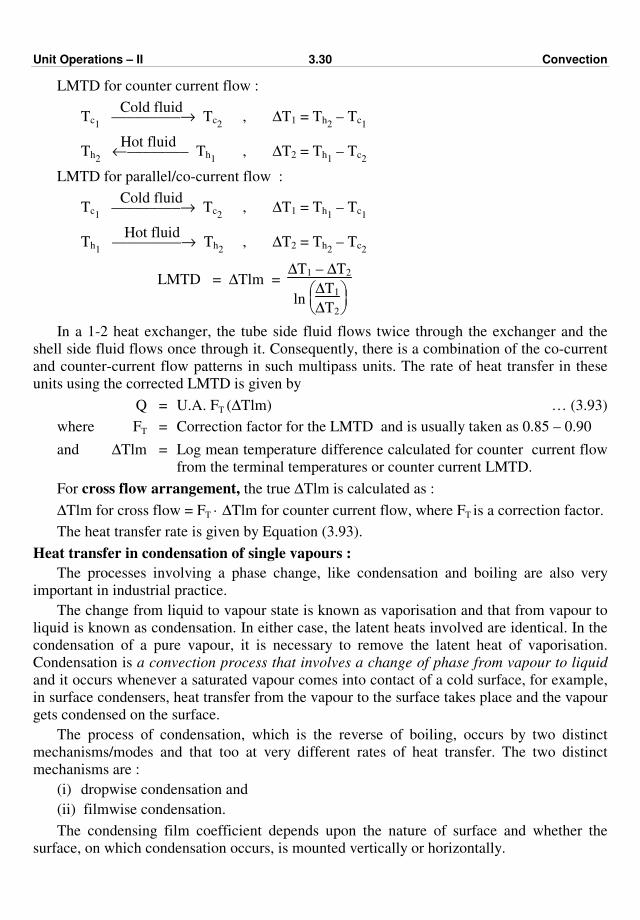
Unit Operations – II 3.30 Convection
LMTD for counter current flow :
Tc1
Cold fluid –––––––––→ Tc2
, ∆T1 = Th2 – Tc1
Th2
Hot fluid ←–––––––– Th1
, ∆T2 = Th1 – Tc2
LMTD for parallel/co-current flow :
Tc1
Cold fluid –––––––––→ Tc2
, ∆T1 = Th1 – Tc1
Th1
Hot fluid –––––––––→ Th2
, ∆T2 = Th2 – Tc2
LMTD = ∆Tlm = ∆T1 – ∆T2
ln
∆T1
∆T2
In a 1-2 heat exchanger, the tube side fluid flows twice through the exchanger and the
shell side fluid flows once through it. Consequently, there is a combination of the co-current
and counter-current flow patterns in such multipass units. The rate of heat transfer in these
units using the corrected LMTD is given by
Q = U.A. FT (∆Tlm) … (3.93)
where FT = Correction factor for the LMTD and is usually taken as 0.85 – 0.90
and ∆Tlm = Log mean temperature difference calculated for counter current flow
from the terminal temperatures or counter current LMTD.
For cross flow arrangement, the true ∆Tlm is calculated as :
∆Tlm for cross flow = FT · ∆Tlm for counter current flow, where FT is a correction factor.
The heat transfer rate is given by Equation (3.93).
Heat transfer in condensation of single vapours :
The processes involving a phase change, like condensation and boiling are also very
important in industrial practice.
The change from liquid to vapour state is known as vaporisation and that from vapour to
liquid is known as condensation. In either case, the latent heats involved are identical. In the
condensation of a pure vapour, it is necessary to remove the latent heat of vaporisation.
Condensation is a convection process that involves a change of phase from vapour to liquid
and it occurs whenever a saturated vapour comes into contact of a cold surface, for example,
in surface condensers, heat transfer from the vapour to the surface takes place and the vapour
gets condensed on the surface.
The process of condensation, which is the reverse of boiling, occurs by two distinct
mechanisms/modes and that too at very different rates of heat transfer. The two distinct
mechanisms are :
(i) dropwise condensation and
(ii) filmwise condensation.
The condensing film coefficient depends upon the nature of surface and whether the
surface, on which condensation occurs, is mounted vertically or horizontally.
Unit Operations – II 3.31 Convection
For filmwise condensation on a vertical surface, the mean heat transfer coefficient is
given by
hm = 0.943
ρ2 g λ k3
µ L ∆Tf
1/4
… (3.94)
where hm - mean heat transfer coefficient over the tube length
L - tube length
g - gravitational acceleration
µ - liquid viscosity
λ - latent heat of vaporisation
k - thermal conductivity of liquid
∆Tf - temperature difference between vapour and metal
For filmwise condensation on a horizontal tube of outside diameter do, the mean heat
transfer coefficient hm is given as :
hm = 0.725
ρ2 g · λ k3
µ do ∆Tf
1/4
… (3.95)
Drop-wise Condensation :
When a saturated vapour comes into contact with a cold surface (a surface at a lower
temperature), it condenses and if condensate does not wet the surface, the droplets are
formed on the surface. These droplets grow and ultimately fall down the surface in a random
fashion under the influence of gravity leaving behind the bare metal surface on which further
condensation takes place. The condensation occurring by this mechanism is known as drop-
wise condensation.
Film-wise Condensation :
When a saturated vapour comes into contact with a cold surface, it condenses and if
condensate wets the surface, it forms a continuous film of condensate, which covers the
entire surface, through which heat must be transferred. The additional vapour is then required
to condense into the liquid film rather than directly on the surface. The condensate ultimately
flows down the surface under the influence of gravity. The condensation occurring by this
mechanism is called as filmwise condensation.
In film-wise condensation, the film covering the surface acts as a resistance to heat
transfer, while in drop-wise condensation, a large portion of the surface is directly exposed to
the vapour. Because of this the heat transfer coefficients (hence the heat transfer rates) in
drop-wise condensation are four to eight times larger than those for filmwise condensation.
Drop-wise condensation needs a physical preparation of surfaces which is very difficult
and needs to be promoted by introducing certain additives into the vapour stream. This type
of condensation is very unstable, i.e., difficult to maintain and also the design methods are
not available. Because of these reasons, dropwise condensation is not common in industry.
In general, smooth, clean, uncontaminated surfaces seem to promote film-wise condensation
and oily or greasy surfaces and presence of dirt on the surfaces, i.e., when impurities are
present and surface is contaminated, seem to promote dropwise condensation.
Unit Operations – II 3.32 Convection
Film-wise condensation is very common and reliable since most surfaces become wetted
after being exposed to the condensing vapours over a period of time and it is difficult to
achieve dropwise condensation and therefore the condensing equipments in use are designed
on the basis of film-wise condensation.
Condensers are widely used in the chemical industry. For example, in the separation of
the constituents of a liquid mixture by distillation, a condenser converts vapours from the top
of the column into liquid distillate and reflux. In power plants the surface condensers are
used for condensing steam from the exhaust of turbines into liquid. The home air
conditioning unit makes a use of air cooled condenser for liquefication of refrigerant.
Effect of non-condensable gases :
If a non-condensable gas is present in condensing vapours, for example, air in the
condensing vapours in a condenser because of say leakage, it hinders the process of heat
transfer. The non-condensable gas collects in the viscinity of condensate surface, and the
condensing vapour has to diffuse through the gas film. The presence of this diffusion
resistance in the process of condensation decreases the rate of condensation far below than
that for a pure material. Presence of about 1% by volume air in the condensing vapours can
reduce the heat transfer coefficient by 60% of its value for no air. Thus, an air vent is always
provided on almost all the condensers to eliminate air from the system.
Difference between drop-wise and film-wise condensation :
Drop-wise condensation Film-wise condensation
1. In drop-wise condensation the
condensate does not wet the surface and
collects in the form of droplets. These
droplets grow for a while and then fall
from the surface, leaving behind the bare
metal surface for further condensation.
1. In film-wise condensation the condensed
liquid wets the surface and forms a
continuous film of condensate on the
surface through which heat transfer takes
place. The condensate flows down the
surface under the action of gravity.
2. Heat transfer coefficients are very high
as the heat does not have to flow through
a film by conduction.
2. Heat transfer coefficients are relatively
very low since the heat does have to
flow through a film by conduction.
3. Oily or greasy surfaces seem to tend
towards drop-wise condensation.
3. Smooth, clean uncontaminated surfaces
seem to tend towards film-wise
condensation.
4. Drop-wise condensation is very difficult
to achieve.
4. Film-wise condensation is easily
obtainable.
5. Drop-wise condensation is unstable and
difficult to maintain, uncommon and so
not desired industrially.
5. Film-wise condensation is stable, easy,
reliable, common and so desired
industrially.
6. Methods for predicting the film
coefficient are not available.
6. Methods for predicting the film
coefficients are available.
7. Heat transfer coefficients and heat
transfer rates are very high.
7. Heat transfer coefficients and heat
transfer rates are low.
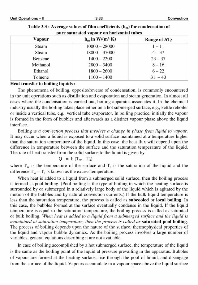
Unit Operations – II 3.33 Convection
Table 3.3 : Average values of film coefficients (hm) for condensation of
pure saturated vapour on horizontal tubes
Vapour hm in W/(m2·K) Range of ∆∆∆∆Tf
Steam
Steam
Benzene
Methanol
Ethanol
Toluene
10000 – 28000
18000 – 37000
1400 – 2200
2800 – 3400
1800 – 2600
1100 – 1400
1 – 11
4 – 37
23 – 37
8 – 16
6 – 22
31 – 40
Heat transfer to boiling liquids :
The phenomena of boiling, opposite/reverse of condensation, is commonly encountered
in the unit operations such as distillation and evaporation and steam generation. In almost all
cases where the condensation is carried out, boiling apparatus associates it. In the chemical
industry usually the boiling takes place either on a hot submerged surface, e.g., kettle reboiler
or inside a vertical tube, e.g., vertical tube evaporator. In boiling practice, initially the vapour
is formed in the form of bubbles and afterwards as a distinct vapour phase above the liquid
interface.
Boiling is a convection process that involves a change in phase from liquid to vapour.
It may occur when a liquid is exposed to a solid surface maintained at a temperature higher
than the saturation temperature of the liquid. In this case, the heat flux will depend upon the
difference in temperature between the surface and the saturation temperature of the liquid.
The rate of heat transfer from the solid surface to the liquid is given by
Q = h (Tw – Ts)
where Tw is the temperature of the surface and Ts is the saturation of the liquid and the
difference Tw – Ts is known as the excess temperature.
When heat is added to a liquid from a submerged solid surface, then the boiling process
is termed as pool boiling. (Pool boiling is the type of boiling in which the heating surface is
surrounded by or submerged in a relatively large body of the liquid which is agitated by the
motion of the bubbles and by natural convection currents.) If the bulk liquid temperature is
less than the saturation temperature, the process is called as subcooled or local boiling. In
this case, the bubbles formed at the surface eventually condense in the liquid. If the liquid
temperature is equal to the saturation temperature, the boiling process is called as saturated
or bulk boiling. When heat is added to a liquid from a submerged surface and the liquid is
maintained at saturation temperature, then the process is called as saturated pool boiling.
The process of boiling depends upon the nature of the surface, thermophysical properties of
the liquid and vapour bubble dynamics. As the boiling process involves a large number of
variables, general equations describing it are not available.
In case of boiling accomplished by a hot submerged surface, the temperature of the liquid
is the same as the boiling point of the liquid at pressure prevailing in the apparatus. Bubbles
of vapour are formed at the heating surface, rise through the pool of liquid, and disengage
from the surface of the liquid. Vapours accumulate in a vapour space above the liquid surface
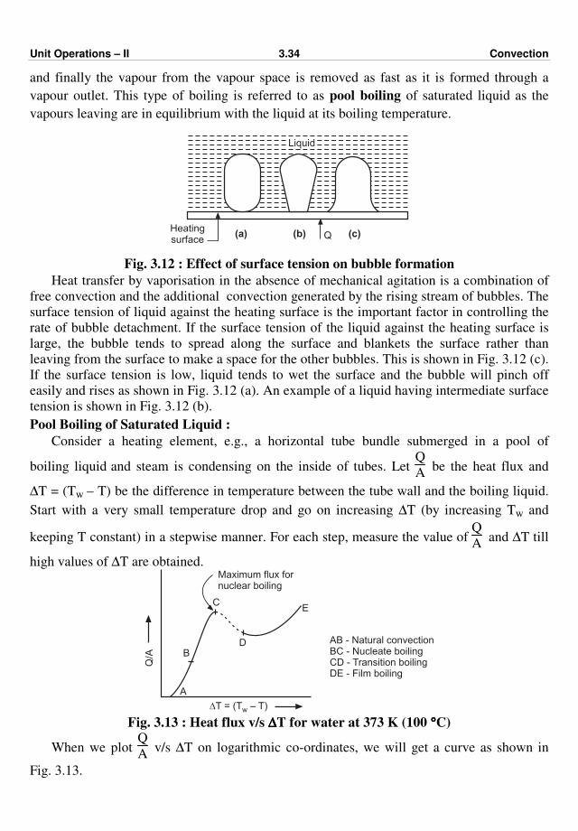
Unit Operations – II 3.34 Convection
and finally the vapour from the vapour space is removed as fast as it is formed through a
vapour outlet. This type of boiling is referred to as pool boiling of saturated liquid as the
vapours leaving are in equilibrium with the liquid at its boiling temperature.
Liquid
Heatingsurface
(a) (b) (c)Q
Fig. 3.12 : Effect of surface tension on bubble formation
Heat transfer by vaporisation in the absence of mechanical agitation is a combination of
free convection and the additional convection generated by the rising stream of bubbles. The
surface tension of liquid against the heating surface is the important factor in controlling the
rate of bubble detachment. If the surface tension of the liquid against the heating surface is
large, the bubble tends to spread along the surface and blankets the surface rather than
leaving from the surface to make a space for the other bubbles. This is shown in Fig. 3.12 (c).
If the surface tension is low, liquid tends to wet the surface and the bubble will pinch off
easily and rises as shown in Fig. 3.12 (a). An example of a liquid having intermediate surface
tension is shown in Fig. 3.12 (b).
Pool Boiling of Saturated Liquid :
Consider a heating element, e.g., a horizontal tube bundle submerged in a pool of
boiling liquid and steam is condensing on the inside of tubes. Let Q
A be the heat flux and
∆T = (Tw – T) be the difference in temperature between the tube wall and the boiling liquid.
Start with a very small temperature drop and go on increasing ∆T (by increasing Tw and
keeping T constant) in a stepwise manner. For each step, measure the value of Q
A and ∆T till
high values of ∆T are obtained.
Q/A
DT = (T – T)w
B
A
C
D
E
Maximum flux fornuclear boiling
AB - Natural convectionBC - Nucleate boilingCD - Transition boilingDE - Film boiling
Fig. 3.13 : Heat flux v/s ∆∆∆∆T for water at 373 K (100 °°°°C)
When we plot Q
A v/s ∆T on logarithmic co-ordinates, we will get a curve as shown in
Fig. 3.13.
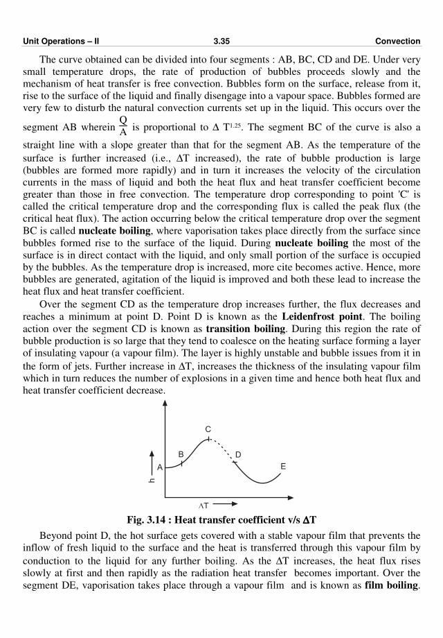
Unit Operations – II 3.35 Convection
The curve obtained can be divided into four segments : AB, BC, CD and DE. Under very
small temperature drops, the rate of production of bubbles proceeds slowly and the
mechanism of heat transfer is free convection. Bubbles form on the surface, release from it,
rise to the surface of the liquid and finally disengage into a vapour space. Bubbles formed are
very few to disturb the natural convection currents set up in the liquid. This occurs over the
segment AB wherein Q
A is proportional to ∆ T1.25. The segment BC of the curve is also a
straight line with a slope greater than that for the segment AB. As the temperature of the
surface is further increased (i.e., ∆T increased), the rate of bubble production is large
(bubbles are formed more rapidly) and in turn it increases the velocity of the circulation
currents in the mass of liquid and both the heat flux and heat transfer coefficient become
greater than those in free convection. The temperature drop corresponding to point 'C' is
called the critical temperature drop and the corresponding flux is called the peak flux (the
critical heat flux). The action occurring below the critical temperature drop over the segment
BC is called nucleate boiling, where vaporisation takes place directly from the surface since
bubbles formed rise to the surface of the liquid. During nucleate boiling the most of the
surface is in direct contact with the liquid, and only small portion of the surface is occupied
by the bubbles. As the temperature drop is increased, more cite becomes active. Hence, more
bubbles are generated, agitation of the liquid is improved and both these lead to increase the
heat flux and heat transfer coefficient.
Over the segment CD as the temperature drop increases further, the flux decreases and
reaches a minimum at point D. Point D is known as the Leidenfrost point. The boiling
action over the segment CD is known as transition boiling. During this region the rate of
bubble production is so large that they tend to coalesce on the heating surface forming a layer
of insulating vapour (a vapour film). The layer is highly unstable and bubble issues from it in
the form of jets. Further increase in ∆T, increases the thickness of the insulating vapour film
which in turn reduces the number of explosions in a given time and hence both heat flux and
heat transfer coefficient decrease.
B
C
D
EA
DT
h
Fig. 3.14 : Heat transfer coefficient v/s ∆∆∆∆T
Beyond point D, the hot surface gets covered with a stable vapour film that prevents the
inflow of fresh liquid to the surface and the heat is transferred through this vapour film by
conduction to the liquid for any further boiling. As the ∆T increases, the heat flux rises
slowly at first and then rapidly as the radiation heat transfer becomes important. Over the
segment DE, vaporisation takes place through a vapour film and is known as film boiling.
Unit Operations – II 3.36 Convection
The relationship between ∆T and h (heat transfer coefficient) from A to E is shown in
Fig. 3.14. In film boiling, the rate of heat transfer is low for a large temperature drop and the
temperature drop is not utilised effectively. Hence, film boiling is not usually desired in
commercial heat transfer equipments and the heat transfer equipments are generally designed
for the temperature drop less than the critical temperature drop.
SOLVED EXAMPLES
Example 3.1 : A hot fluid enters a double pipe heat exchanger at a temperature of
423 K (150 oC) and is to be cooled to 367 K (94oC) by a cold fluid entering at 311 K (38oC)
and heated to 339 K (66oC). Shall they be directed in parallel or counter-current flow ?
Solution : (I) For counter current flow :
Th1 , 423 K Hot fluid
–––––––––––→367 K, Th2
Tc2 , 339 K
Cold fluid–––––––––––→311 K, Tc1
Th1 – temperature of hot fluid at inlet = 423 K
Th2 – temperature of hot fluid at outlet = 367 K
Tc1 – temperature of cold fluid at inlet = 311 K
Tc2 – temperature of cold fluid at outlet = 339 K
∆T2 = Th2 – Tc1
= 367 – 311 = 56 K
∆T1 = Th1 – Tc2
= 423 – 339 = 84 K
Log mean temperature difference (LMTD) for counter current flow is given by
∆Tlm = ∆T1 – ∆T2
ln (∆T1/∆T2) =
84 – 56
ln
84
56
= 69 K
LMTD (counter-current flow) = 69 K
(II) For parallel flow :
423 K hot fluid
–––––––→ 367 K
311 K cold fluid
–––––––→ 339 K
∆T2 = Th2 – Tc2
= 367 – 339 = 28 K
∆T1 = Th1 – Tc1
= 423 – 311 = 112 K
Log mean temperature difference for parallel flow is given by
∆Tlm = ∆T1 – ∆T2
ln
∆T1
∆T2
= 112 – 28
ln
112
28
LMTD (parallel flow) = 60.6 K ………… Ans.
Since the LMTD for the counter current flow is more than that for the co-current/parallel
flow, the fluids must be directed in the counter current fashion.
Unit Operations – II 3.37 Convection
Example 3.2 : Thermic fluid flowing at a rate of 5000 kg/h is to be cooled from
423 K (150oC) to 363 K (90oC) by circulating water at a rate of 15000 kg/h. If the water is
available at 303 K (30oC), find the outlet temperature of water.
Data : Specific heat of thermic fluid = 2.72 kJ/(kg·K)
Specific heat of water = 4.187 kJ/(kg·K)
Solution : Basis : 5000 kg/h of thermic fluid.
At steady state, the heat given out by the thermic fluid is equal to the heat gained by the
circulating water. Therefore,
Q = ·mt Cpt
(T1 – T2) = ·mw Cpw
(t2 – t1)
where, ·mt = 5000 kg/h (mass flow rate of thermic fluid)
Cpt = 2.72 kJ/(kg·K)
T1 = Th1 = Inlet temperature of thermic fluid
= 423 K
T2 = Th2 = Outlet temperature of thermic fluid
= 363 K
·mw = 15000 kg/h (mass flow rate of circulating water)
Cpw = 4.187 kJ/(kg·K)
t1 = Tc1 = Inlet temperature of water
= 303 K
t2 = Tc2 = Outlet temperature of water = ?
We have :
·mt Cpt
(T1 – T2) = ·mw Cpw
(t2 – t1)
5000 × 2.72 (423 – 363) = 15000 × 4.187 (t2 – 303)
Solving for t2 gives
t2 = 316 K (43oC)
Outlet temperature of water = 316 K (43°°°°C) … Ans.
Example 3.3 : Cold fluid is flowing through the heat exchanger at a rate of 15 m3/h.
It enters the heat exchanger at 303 K [30oC] and leaves at 328 K [55oC]. A hot thermic fluid
enters the heat exchanger at a rate of 21 m3/h at a temperature of 388 K [115oC]. Find the
area of heat transfer required assuming the flow to be counter current and overall heat
transfer coefficient be 3490 W/(m2·K).
Data : Density of cold fluid = 1000 kg/m3
Density of thermic fluid = 950 kg/m3
Specific heat of cold fluid = 4.187 kJ/(kg·K)
Specific heat of thermic fluid = 2.93 kJ/(kg·K)
Unit Operations – II 3.38 Convection
Solution : Basis : 21 m3/h of thermic fluid
·mt = mass flow rate of thermic fluid
= volumetric flow rate × density
= 21 × 950
= 19950 kg/h
Volumetric flow rate of cold fluid = 15 m3/h
Similarly, ·mc = mass flow rate of the cold fluid
= 15 × 1000
= 15000 kg/h
T1 = Inlet (initial) temperature of the thermic fluid = 388 K
T2 = Outlet temperature of the thermic fluid, K
t1 = Initial temperature of the cold fluid = 303 K
t2 = Outlet temperature of the cold fluid = 328 K
Let us calculate T2.
At steady state, the heat gained by the cold fluid is equal to heat given out by the thermic
fluid. Therefore,
Q = ·mt · Cpt
(T1 – T2) = ·mc · Cpc
(t2 – t1)
19950 × 2.93 × (388 – T2) = 15000 × 4.187 (328 – 303)
∴ T2 = 361.2 K (88.2oC)
For counter current flow :
388 K Thermic fluid––––––––––→ 361.2 K
328 K Cold fluid←–––––– 303 K
∴ ∆T1 = T1 – t2 = 388 – 328 = 60 K
∆T2 = T2 – t1 = 361.2 – 303 = 58.2 K
Let us calculate LMTD.
∴ ∆Tlm = LMTD
= (∆T2 – ∆T1)
ln
∆T2
∆T1
= 60 – 58.2
ln
60
58.2
= 59.1 K
Let us calculate the rate of heat transfer based on the thermic fluid.
Q = Rate of heat transfer
= ·mt · Cpt
(T1 – T2)
= 19950 × 2.93 × (388 – 361.2)
= 1566554 kJ/h
= 435154 J/s ≡ 435154 W
Unit Operations – II 3.39 Convection
Let us find the area of heat transfer.
We know : Q = U.A. ∆T lm
where U = overall heat transfer coefficient
= 3490 W/(m2·K)
∆Tlm = LMTD = 59.1 K
A = area of heat transfer in m2 = ?
Q = Rate of heat transfer
= 435154 W
∴ 435154 = 3490 × A × 59.1
A = Area of heat transfer
= 2.11 m2 … Ans.
Example 3.4 : Calculate the heat transfer area of a 1-2 heat exchanger from the
following data : Inlet and outlet temperatures of the hot fluid are 423 K (150oC) and
353 K (80oC) respectively. Inlet and outlet temperatures of the cold fluid are 303 K (30oC)
and 318 K (45oC) respectively.
∴ Overall heat transfer coefficient = 4100 W/(m2·K)
Heat loss = 407 kW
L.M.T.D. correction factor = 0.84
Solution : The rate of heat loss is given by
Q = U.A. FT ∆Tlm
Given : Q = 407 kW = 407 × 103 W
U = Overall heat transfer coefficient
= 4100 W/(m2·K)
A = Area of heat transfer, m2
∆Tlm = log mean temperature difference for counter current flow
FT = L.M.T.D. correction factor for 1-2 heat exchanger
= 0.84
Let us find LMTD for counter current flow.
423 K hot fluid
→ 353 K
318 K cold fluid← 303 K
∆T1 = Th1 – Tc2 = 423 – 318 = 105 K
∆T2 = Th2 – Tc1 = 353 – 303 = 50 K
Unit Operations – II 3.40 Convection
∆Tlm = LMTD
= ∆T1 – ∆T2
ln
∆T1
∆T2
= (105 – 50)
ln
105
50
= 74.13 K
We have : Q = U.A. FT · ∆Tlm
407 × 103 = 4100 × A × 0.84 × 74.13
A = 1.594 m2 ~– 1.6 m2
Area of heat transfer = 1.6 m2 … Ans.
Example 3.5 : Calculate the inside heat transfer coefficient for a fluid flowing at a rate
of 300 cm3/s through a 20 mm inside diameter tube of heat exchanger.
Data : Viscosity of flowing fluid = 0.8 (N.s)/m2
Density of flowing fluid = 1.1 g/cm3
Specific heat of fluid = 1.26 kJ/(kg·K)
Thermal conductivity of fluid = 0.384 W/(m·K)
Viscosity at wall temperature = 1.0 (N.s)/m2
Length of heat exchanger = 5 m
Solution : Basis : 300 cm3/s of volumetric flow rate of fluid
Volumetric flow rate = 300 cm3/s
= 300 × 10–6 m3/s
Density of the flowing fluid = 1.1 g/cm3
Density of the flowing fluid = 1100 kg/m3
Mass flow rate of the flowing fluid = 300 × 10–6 × 1100 = 0.33 kg/s
Inside diameter of the pipe = Di = 20 mm = 0.02 m
Area of pipe (cross section) = π/4 D2
i
= π/4 (0.02)2 = 3.14 × 10⁻⁴ m2
Velocity of flowing fluid = Volumetric flow rate
Cross section area
u = 300 × 10–6
3.14 × 10–4 = 0.955 m/s
Let us calculate NRe. NRe = Reynolds number
= Diuρ
µ

Unit Operations – II 3.41 Convection
where Di = 0.02 m
u = 0.955 m/s
ρ = 1100 kg/m3
µ = 0.8 (N.s)/m2 = 0.8 kg/(m.s)
NRe = 0.02 × 0.955 × 1100
0.8 = 26.26
As the Reynolds number is less than 2100, the flow is laminar.
Let us calculate NPr.
NPr = Cp µ
k
where, Cp = 1.26 kJ/(kg·K) = 1.26 × 10³ J/(kg·K)
µ = 0.8 kg/(m.s)
k = 0.384 W/(m·K)
NPr = 1.26 × 103 × 0.8
0.384 = 2625
NRe · NPr · D
L = 26.26 × 2625 ×
0.02
5 = 275.73
µw = 1.0 (N.s)/m2 = 1.0 kg/(m·s)
Let us calculate hi.
The empirical relation applicable for laminar flow is
NNu = 1.86
NRe · NPr · D
L
1/3
µ
µw
0.14
NNu = 1.86
(26.26) (2625) × 0.02
5
1/3
×
0.8
1.0
0.14
= 11.71
We have : NNu = hi Di
k
where hi is the inside heat transfer coefficient.
∴ 11.71 = hi × 0.02
0.384
hi = 1225 W/(m2·K) … Ans.
Example 3.6 : Calculate the heat transfer coefficient for fluid flowing through a tube
having inside diameter 40 mm at a rate of 5500 kg/h. Assume that the fluid is being heated.
Data : Properties of fluid at mean bulk temperature :
Viscosity of flowing fluid = 0.004 (N.s)/m2
Density of flowing fluid = 1.07 g/cm3
Specific heat of flowing fluid = 2.72 kJ/(kg.K)
Thermal conductivity of flowing fluid = 0.256 W/(m·K)
Make use of Dittus – Boelter equation.
Unit Operations – II 3.42 Convection
Solution : Basis : 5500 kg/h of fluid flowing through the tube
Mass flow rate = ·m = 5500 kg/h =
5500
3600 = 1.53 kg/s
Density of the fluid = ρ = 1.07 g/cm3 = 1070 kg/m3
Volumetric flow rate = ·m /ρ =
1.53
1070 = 1.43 × 10⁻³ m3/s
Cross-sectional area of the tube = π4
D2
i
where Di = 40 mm = 0.04 m
A = π4
(0.040) 2 = 1.256 × 10⁻³ m2
Let us calculate u.
Velocity of the flowing fluid = u = 1.43 × 10⁻³
1.256 × 10–3 = 1.14 m/s
Let us calculate NRe.
Reynolds number = NRe = Diuρ
µ
where Di = inside diameter of pipe
= 40 mm = 0.04 m
ρ = 1070 kg/m3
u = 1.14 m/s
µ = Viscosity
= 0.004 (N.s)/m2 = 0.004 kg/(m·s)
NRe = 0.04 × 1.14 × 1070
0.004 = 12198
Let us calculate NPr.
NPr = Cp · µ
k
Cp = 2.72 kJ/(kg·K) = 2.72 × 10³ J/(kg·K)
k = 0.256 W/(m·K)
µ = 0.004 kg/(m·s)
NPr = 2.72 × 103 × 0.004
0.256 = 42.5
As NRe is greater than 10000, the flow is turbulent.
Let us obtain hi.
The empirical relationship for turbulent flow, i.e., the Dittus–Boelter equation for heating
is
NNu = 0.023 (NRe)0.8 (NPr)0.4
Unit Operations – II 3.43 Convection
NNu = 0.023 (12198)0.8 (42.5)0.4 = 191.5
NNu = Nusselt number
hi Di
k = 191.5
where, hi = inside heat transfer coefficient
Di = inside diameter of pipe
= 0.04 m
k = thermal conductivity of fluid
= 0.256 W/(m·K)
hi (0.04)
0.256 = 191.5
hi = 1225.5 W/(m2·K) … Ans.
Example 3.7 : Calculate the overall heat transfer coefficient from the following data :
Inside heat transfer coefficient = 5800 W/(m2·K)
Outside heat transfer coefficient = 1750 W/(m2·K)
Outside diameter of tube = 30 mm
Inside diameter of tube = 20 mm
Thermal conductivity of metal wall = 46.52 W/(m·K)
Solution : The relationship among U, hi, ho and k/x is
1
U =
1
ho +
1
hi +
1
k/x … (1)
where U = overall heat transfer coefficient
ho = outside heat transfer coefficient
= 1750 W/(m2·K)
hi = inside heat transfer coefficient
= 5800 W/(m2·K)
k = thermal conductivity of the metal wall
= 46.52 W/(m·K)
x = thickness of the metal wall of tube
= (O.D. – I.D.) / 2
= (30 – 20)
2 = 5 mm = 0.005 m
Substituting the values in Equation (1) gives
1
U =
1
1750 +
1
5800 +
1
46.52
0.005
U = 1175 W/(m2·K)
Overall heat transfer coefficient = 1175 W/(m2·K) … Ans.
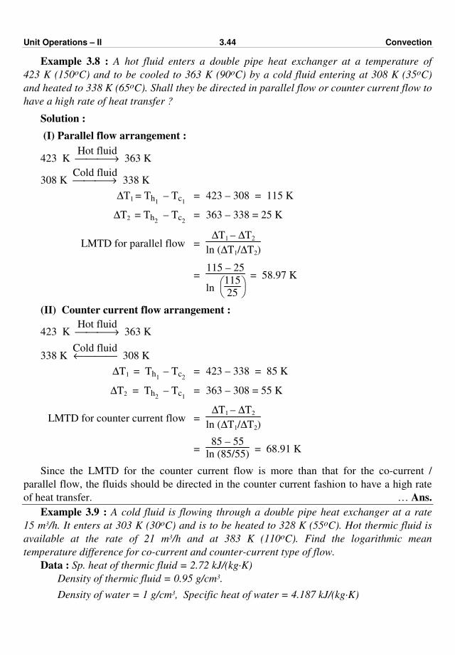
Unit Operations – II 3.44 Convection
Example 3.8 : A hot fluid enters a double pipe heat exchanger at a temperature of
423 K (150oC) and to be cooled to 363 K (90oC) by a cold fluid entering at 308 K (35oC)
and heated to 338 K (65oC). Shall they be directed in parallel flow or counter current flow to
have a high rate of heat transfer ?
Solution :
(I) Parallel flow arrangement :
423 K Hot fluid→ 363 K
308 K Cold fluid→ 338 K
∆T1 = Th1 – Tc1
= 423 – 308 = 115 K
∆T2 = Th2 – Tc2
= 363 – 338 = 25 K
LMTD for parallel flow = ∆T1 – ∆T2
ln (∆T1/∆T2)
= 115 – 25
ln
115
25
= 58.97 K
(II) Counter current flow arrangement :
423 K Hot fluid→ 363 K
338 K Cold fluid← 308 K
∆T1 = Th1 – Tc2
= 423 – 338 = 85 K
∆T2 = Th2 – Tc1
= 363 – 308 = 55 K
LMTD for counter current flow = ∆T1 – ∆T2
ln (∆T1/∆T2)
= 85 – 55
ln (85/55) = 68.91 K
Since the LMTD for the counter current flow is more than that for the co-current /
parallel flow, the fluids should be directed in the counter current fashion to have a high rate
of heat transfer. … Ans.
Example 3.9 : A cold fluid is flowing through a double pipe heat exchanger at a rate
15 m3/h. It enters at 303 K (30oC) and is to be heated to 328 K (55oC). Hot thermic fluid is
available at the rate of 21 m3/h and at 383 K (110oC). Find the logarithmic mean
temperature difference for co-current and counter-current type of flow.
Data : Sp. heat of thermic fluid = 2.72 kJ/(kg·K)
Density of thermic fluid = 0.95 g/cm3.
Density of water = 1 g/cm3, Specific heat of water = 4.187 kJ/(kg·K)
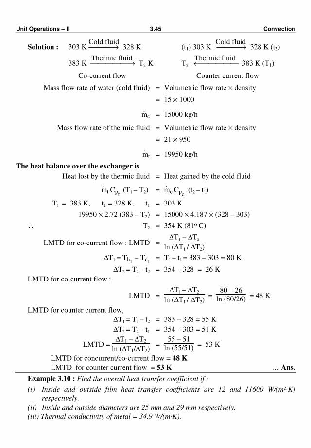
Unit Operations – II 3.45 Convection
Solution : 303 K Cold fluid→ 328 K (t1) 303 K
Cold fluid → 328 K (t2)
383 K Thermic fluid
→ T2 K T2
Thermic fluid ← 383 K (T1)
Co-current flow Counter current flow
Mass flow rate of water (cold fluid) = Volumetric flow rate × density
= 15 × 1000
·mc = 15000 kg/h
Mass flow rate of thermic fluid = Volumetric flow rate × density
= 21 × 950
·mt = 19950 kg/h
The heat balance over the exchanger is
Heat lost by the thermic fluid = Heat gained by the cold fluid
·mt Cpt
(T1 – T2) = ·mc Cpc
(t2 – t1)
T1 = 383 K, t2 = 328 K, t1 = 303 K
19950 × 2.72 (383 – T2) = 15000 × 4.187 × (328 – 303)
∴ T2 = 354 K (81o C)
LMTD for co-current flow : LMTD = ∆T1 – ∆T2
ln (∆T1 / ∆T2)
∆T1 = Th1 – Tc1
= T1 – t1 = 383 – 303 = 80 K
∆T2 = T2 – t2 = 354 – 328 = 26 K
LMTD for co-current flow :
LMTD = ∆T1 – ∆T2
ln (∆T1 / ∆T2) =
80 – 26
ln (80/26) = 48 K
LMTD for counter current flow,
∆T1 = T1 – t2 = 383 – 328 = 55 K
∆T2 = T2 – t1 = 354 – 303 = 51 K
LMTD = ∆T1 – ∆T2
ln (∆T1/∆T2) =
55 – 51
ln (55/51) = 53 K
LMTD for concurrent/co-current flow = 48 K
LMTD for counter current flow = 53 K … Ans.
Example 3.10 : Find the overall heat transfer coefficient if :
(i) Inside and outside film heat transfer coefficients are 12 and 11600 W/(m2·K)
respectively.
(ii) Inside and outside diameters are 25 mm and 29 mm respectively.
(iii) Thermal conductivity of metal = 34.9 W/(m·K).
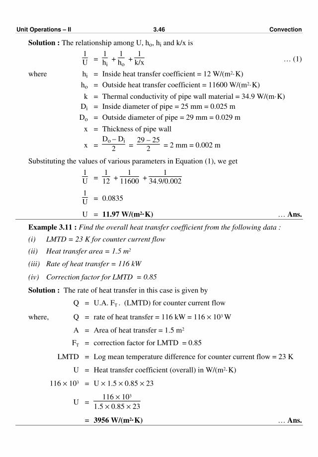
Unit Operations – II 3.46 Convection
Solution : The relationship among U, ho, hi and k/x is
1
U =
1
hi +
1
ho +
1
k/x … (1)
where hi = Inside heat transfer coefficient = 12 W/(m2·K)
ho = Outside heat transfer coefficient = 11600 W/(m2·K)
k = Thermal conductivity of pipe wall material = 34.9 W/(m·K)
Di = Inside diameter of pipe = 25 mm = 0.025 m
Do = Outside diameter of pipe = 29 mm = 0.029 m
x = Thickness of pipe wall
x = Do – Di
2 =
29 – 25
2 = 2 mm = 0.002 m
Substituting the values of various parameters in Equation (1), we get
1
U =
1
12 +
1
11600 +
1
34.9/0.002
1
U = 0.0835
U = 11.97 W/(m2·K) … Ans.
Example 3.11 : Find the overall heat transfer coefficient from the following data :
(i) LMTD = 23 K for counter current flow
(ii) Heat transfer area = 1.5 m2
(iii) Rate of heat transfer = 116 kW
(iv) Correction factor for LMTD = 0.85
Solution : The rate of heat transfer in this case is given by
Q = U.A. FT . (LMTD) for counter current flow
where, Q = rate of heat transfer = 116 kW = 116 × 103 W
A = Area of heat transfer = 1.5 m2
FT = correction factor for LMTD = 0.85
LMTD = Log mean temperature difference for counter current flow = 23 K
U = Heat transfer coefficient (overall) in W/(m2·K)
116 × 103 = U × 1.5 × 0.85 × 23
U = 116 × 103
1.5 × 0.85 × 23
= 3956 W/(m2·K) … Ans.

Unit Operations – II 3.47 Convection
Example 3.12 : Find the inside heat transfer coefficient using Sieder-Tate equation for
turbulent flow.
Data : I.d. of tube = 20 mm, NRe = 15745
Viscosity of fluid at bulk mean temperature = 550 × 10–5 Pa·s
Viscosity of fluid at average wall temperature = 900 × 10–6 Pa·s
Prandtl number = 36, Thermal conductivity of fluid = k = 0.25 W/(m·K)
Solution : The Sieder-Tate equation is
hi Di
k = 0.023 (NRe)0.8 (NPr)1/3
µ
µw
0.14 … (1)
where,
µ
µw
0.14
= Sieder-Tate correction factor
NRe = Reynolds number = 15745
NPr = Prandtl number = 36
hi = inside heat transfer coefficient, W/(m2·K)
Di = inside diameter of pipe = 20 mm = 0.002 m
k = Thermal conductivity of fluid = 0.25 W/(m·K)
µ = 550 × 10–6 Pa·s
µw = 900 × 10–6 Pa·s
Substituting the values in Equation (1), we get
hi (0.02)
0.25 = 0.023 × (15745)0.8 (36)1/3 ×
550 × 10–6
900 × 10–6
0.14
hi (0.02)
0.25 = 0.023 × 2278.84 × 3.3 × 0.933
hi (0.02)
0.25 = 161.37
hi = 2017
Inside heat transfer
coefficient = 2017 W/(m2·K) … Ans.
Example 3.13 : Water enters a two-fluid heat exchanger at 328 K and leaves at 358 K.
Hot gases enter at 578 K and leave at 433 K. If the total heat transfer area is 500 m2 and the
overall heat transfer coefficient is 700 W/(m2·K), determine the total heat transferred for
(i) parallel flow and
(ii) counter current flow of the two fluids.
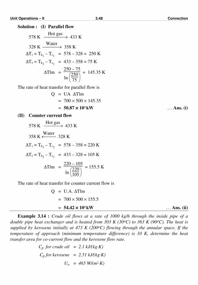
Unit Operations – II 3.48 Convection
Solution : (I) Parallel flow
578 K Hot gas
→ 433 K
328 K Water
→ 358 K
∆T1 = Th1 – Tc1 = 578 – 328 = 250 K
∆T2 = Th2 – Tc1 = 433 – 358 = 75 K
∆Tlm = 250 – 75
ln
250
75
= 145.35 K
The rate of heat transfer for parallel flow is
Q = UA ∆Tlm
= 700 × 500 × 145.35
= 50.87 ×××× 103 kW … Ans. (i)
(II) Counter current flow
578 K Hot gas
→ 433 K
358 K Water
← 328 K
∆T1 = Th1 – Tc2 = 578 – 358 = 220 K
∆T2 = Th2 – Tc1 = 433 – 328 = 105 K
∆Tlm = 220 – 105
ln
220
105
= 155.5 K
The rate of heat transfer for counter current flow is
Q = U.A. ∆Tlm
= 700 × 500 × 155.5
= 54.42 ×××× 103 kW … Ans. (ii)
Example 3.14 : Crude oil flows at a rate of 1000 kg/h through the inside pipe of a
double pipe heat exchanger and is heated from 303 K (30oC) to 363 K (90oC). The heat is
supplied by kerosene initially at 473 K (200oC) flowing through the annular space. If the
temperature of approach (minimum temperature difference) is 10 K, determine the heat
transfer area for co-current flow and the kerosene flow rate.
Cp for crude oil = 2.1 kJ/(kg·K)
Cp for kerosene = 2.51 kJ/(kg·K)
Uo = 465 W/(m2·K)
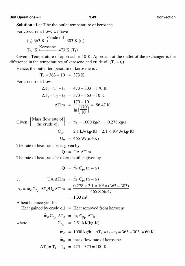
Unit Operations – II 3.49 Convection
Solution : Let T be the outlet temperature of kerosene.
For co-current flow, we have
(t2) 363 K Crude oil← 303 K (t1)
T2, K Kerosene← 473 K (T1)
Given : Temperature of approach = 10 K. Approach at the outlet of the exchanger is the
difference in the temperatures of kerosene and crude oil (T2 – t2).
Hence, the outlet temperature of kerosene is :
T2 = 363 + 10 = 373 K
For co-current flow :
∆T1 = T1 – t1 = 473 – 303 = 170 K
∆T2 = T2 – t2 = 373 – 363 = 10 K
∆Tlm = 170 – 10
ln
170
10
= 56.47 K
Given :
Mass flow rate of
the crude oil = ·mc = 1000 kg/h = 0.278 kg/s
Cpc = 2.1 kJ/(kg·K) = 2.1 × 10³ J/(kg·K)
Uo = 465 W/(m2·K)
The rate of heat transfer is given by
Q = UA ∆Tlm
The rate of heat transfer to crude oil is given by
Q = ⋅mc Cpc
(t2 – t1)
∴ UA ∆Tlm = ⋅mc Cpc
(t2 – t1)
Ao = ·mc Cpc
∆Tc/Uo ∆Tlm = 0.278 × 2.1 × 103 × (363 – 303)
465 × 56.47
= 1.33 m2
A heat balance yields :
Heat gained by crude oil = Heat removed from kerosene
·mc Cpc
∆Tc = ·mk Cpk
∆Tk
where Cpk = 2.51 kJ/(kg·K)
·mc = 1000 kg/h, ∆Tc = t2 – t1 = 363 – 303 = 60 K
·mk = mass flow rate of kerosene
∆Tk = T1 – T2 = 473 – 373 = 100 K

Unit Operations – II 3.50 Convection
·mk =
⋅m Cpc
∆Tc
Cpk ∆Tk
= 1000 × 2.1 × 60
2.51 × 100
= 502 kg/h
Mass flow rate of kerosene = 502 kg/h … Ans.
Example 3.15 : Methyl alcohol flowing in the inner pipe of a double pipe heat exchanger
is cooled with water flowing in the outer pipe. The inside and outside diameters of the inner
pipe are 26 mm and 35 mm, respectively. The thermal conductivity of steel is 50 W/(m·K).
The individual film coefficients and fouling factors are :
Alcohol coefficients = 250 W/(m2·K)
Water coefficients = 500 W/(m2·K)
Inside fouling factor = 0.86 × 10⁻³ (m2·K)/W
Outside fouling factor = 1.7 × 10⁻³ (m2·K)/W
Calculate the overall coefficients based on the outside area of the inner pipe including
dirt factors and excluding dirt factors.
Solution :
Inside diameter = Di = 26 mm = 0.026 m
Outside diameter = Do = 35 mm = 0.035 m
xw = 35 – 26
2 = 4.5 mm = 0.0045 m
Dw = log mean diameter
= Do – Di
ln
Do
Di
= 0.035 – 0.026
ln
0.035
0.026
= 0.0303 m
k for steel = 50 W/(m·K)
Overall heat transfer coefficient based on the outside area of inner pipe (Uo) is given by
1
U =
1
ho +
1
hi ·
Do
Di +
xw · Do
k · Dw + Rdo + Rdi
Do
Di
This equation includes dirt factors.
1
Uo =
1
500 +
0.035
0.026 ×
1
250 +
0.0045
50 ×
0.035
0.0303 + 1.7 × 10⁻³ + 0.86 × 10⁻³
0.035
0.026
Uo (inclusive of dirt factors) = 96.65 W/(m2·K) … Ans.
Uo excluding dirt factors is
1
Uo =
1
ho +
1
hi ×
Do
Di +
xw · Do
k · Dw
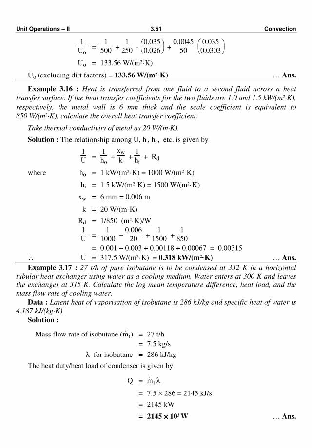
Unit Operations – II 3.51 Convection
1
Uo =
1
500 +
1
250 ·
0.035
0.026 +
0.0045
50
0.035
0.0303
Uo = 133.56 W/(m2·K)
Uo (excluding dirt factors) = 133.56 W/(m2·K) … Ans.
Example 3.16 : Heat is transferred from one fluid to a second fluid across a heat
transfer surface. If the heat transfer coefficients for the two fluids are 1.0 and 1.5 kW/(m2·K),
respectively, the metal wall is 6 mm thick and the scale coefficient is equivalent to
850 W/(m2·K), calculate the overall heat transfer coefficient.
Take thermal conductivity of metal as 20 W/(m·K).
Solution : The relationship among U, hi, ho, etc. is given by
1
U =
1
ho +
xw
k +
1
hi + Rd
where ho = 1 kW/(m2·K) = 1000 W/(m2·K)
hi = 1.5 kW/(m2·K) = 1500 W/(m2·K)
xw = 6 mm = 0.006 m
k = 20 W/(m·K)
Rd = 1/850 (m2·K)/W
1
U =
1
1000 +
0.006
20 +
1
1500 +
1
850
= 0.001 + 0.003 + 0.00118 + 0.00067 = 0.00315
∴ U = 317.5 W/(m2·K) = 0.318 kW/(m2·K) … Ans.
Example 3.17 : 27 t/h of pure isobutane is to be condensed at 332 K in a horizontal
tubular heat exchanger using water as a cooling medium. Water enters at 300 K and leaves
the exchanger at 315 K. Calculate the log mean temperature difference, heat load, and the
mass flow rate of cooling water.
Data : Latent heat of vaporisation of isobutane is 286 kJ/kg and specific heat of water is
4.187 kJ/(kg·K).
Solution :
Mass flow rate of isobutane (.
m1) = 27 t/h
= 7.5 kg/s
λ for isobutane = 286 kJ/kg
The heat duty/heat load of condenser is given by
Q = ·m1 λ
= 7.5 × 286 = 2145 kJ/s
= 2145 kW
= 2145 ×××× 103 W … Ans.
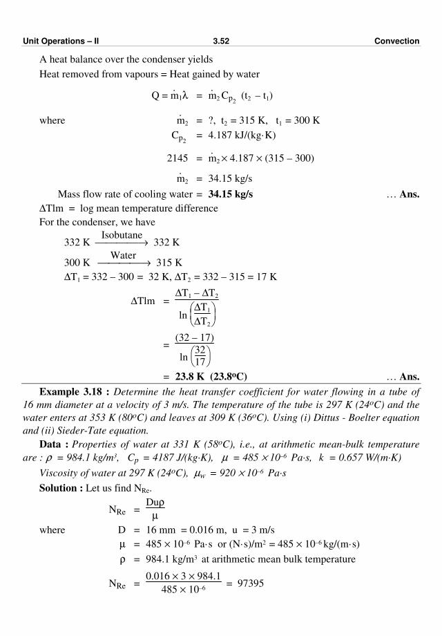
Unit Operations – II 3.52 Convection
A heat balance over the condenser yields
Heat removed from vapours = Heat gained by water
Q = ·m1λ =
·m2 Cp2
(t2 – t1)
where ·m2 = ?, t2 = 315 K, t1 = 300 K
Cp2 = 4.187 kJ/(kg·K)
2145 = ·m2 × 4.187 × (315 – 300)
·m2 = 34.15 kg/s
Mass flow rate of cooling water = 34.15 kg/s … Ans.
∆Tlm = log mean temperature difference
For the condenser, we have
332 K Isobutane
→ 332 K
300 K Water
→ 315 K
∆T1 = 332 – 300 = 32 K, ∆T2 = 332 – 315 = 17 K
∆Tlm = ∆T1 – ∆T2
ln
∆T1
∆T2
= (32 – 17)
ln
32
17
= 23.8 K (23.8oC) … Ans.
Example 3.18 : Determine the heat transfer coefficient for water flowing in a tube of
16 mm diameter at a velocity of 3 m/s. The temperature of the tube is 297 K (24oC) and the
water enters at 353 K (80oC) and leaves at 309 K (36oC). Using (i) Dittus - Boelter equation
and (ii) Sieder-Tate equation.
Data : Properties of water at 331 K (58oC), i.e., at arithmetic mean-bulk temperature
are : ρ = 984.1 kg/m3, Cp = 4187 J/(kg·K), µ = 485 × 10–6 Pa·s, k = 0.657 W/(m·K)
Viscosity of water at 297 K (24oC), µw = 920 × 10–6 Pa·s
Solution : Let us find NRe.
NRe = Duρ
µ
where D = 16 mm = 0.016 m, u = 3 m/s
µ = 485 × 10–6 Pa·s or (N·s)/m2 = 485 × 10–6 kg/(m·s)
ρ = 984.1 kg/m3 at arithmetic mean bulk temperature
NRe = 0.016 × 3 × 984.1
485 × 10–6 = 97395
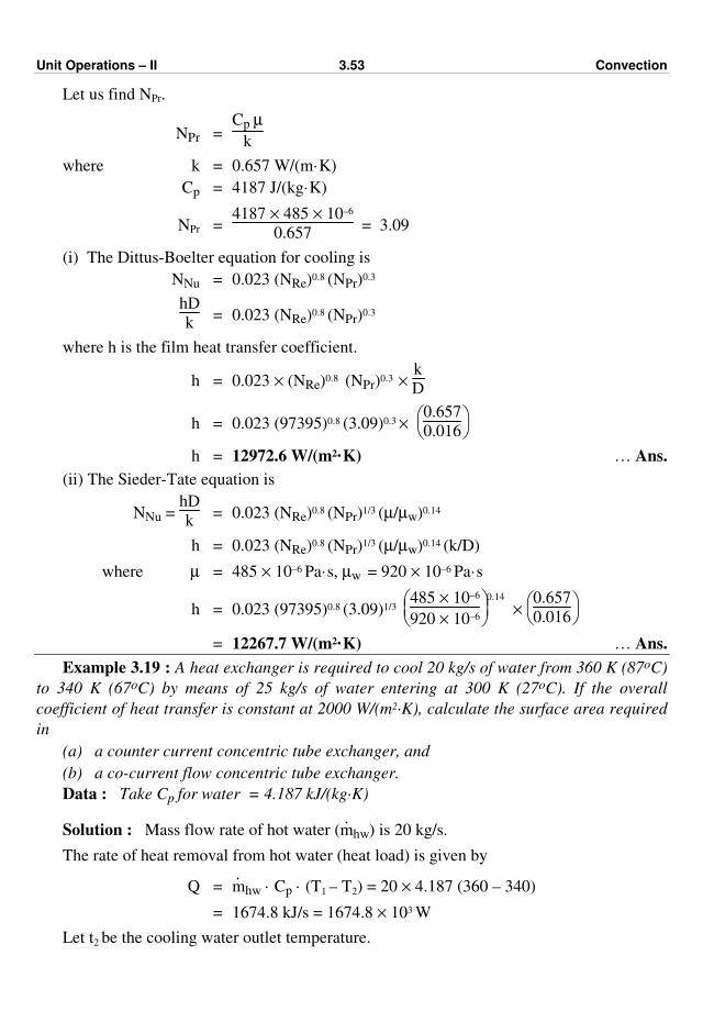
Unit Operations – II 3.53 Convection
Let us find NPr.
NPr = Cp µ
k
where k = 0.657 W/(m·K)
Cp = 4187 J/(kg·K)
NPr = 4187 × 485 × 10–6
0.657 = 3.09
(i) The Dittus-Boelter equation for cooling is
NNu = 0.023 (NRe)0.8 (NPr)0.3
hD
k = 0.023 (NRe)0.8 (NPr)0.3
where h is the film heat transfer coefficient.
h = 0.023 × (NRe)0.8 (NPr)0.3 × k
D
h = 0.023 (97395)0.8 (3.09)0.3 ×
0.657
0.016
h = 12972.6 W/(m2·K) … Ans.
(ii) The Sieder-Tate equation is
NNu = hD
k = 0.023 (NRe)0.8 (NPr)1/3 (µ/µw)0.14
h = 0.023 (NRe)0.8 (NPr)1/3 (µ/µw)0.14 (k/D)
where µ = 485 × 10–6 Pa·s, µw = 920 × 10–6 Pa·s
h = 0.023 (97395)0.8 (3.09)1/3
485 × 10–6
920 × 10–6
0.14
×
0.657
0.016
= 12267.7 W/(m2·K) … Ans.
Example 3.19 : A heat exchanger is required to cool 20 kg/s of water from 360 K (87oC)
to 340 K (67oC) by means of 25 kg/s of water entering at 300 K (27oC). If the overall
coefficient of heat transfer is constant at 2000 W/(m2·K), calculate the surface area required
in
(a) a counter current concentric tube exchanger, and
(b) a co-current flow concentric tube exchanger.
Data : Take Cp for water = 4.187 kJ/(kg·K)
Solution : Mass flow rate of hot water (.
mhw) is 20 kg/s.
The rate of heat removal from hot water (heat load) is given by
Q = ·mhw · Cp · (T1 – T2) = 20 × 4.187 (360 – 340)
= 1674.8 kJ/s = 1674.8 × 103 W
Let t2 be the cooling water outlet temperature.

Unit Operations – II 3.54 Convection
The rate of heat gained by cold water is given by
Q = ·mcw Cp (t2 – t1)
But rate of heat removal = rate of heat gained
∴ 1674.8 = 25 × 4.187 (t2 – 300)
t2 = 316 K (43o C)
(I) Counter current flow :
(360 K) T1 ––→ T2 (340 K)
(316 K) t2 ←––– t1 (300 K)
∆T1 = T1 – t2 = 360 – 316 = 44 K
∆T2 = T2 – t1 = 340 – 300 = 40 K
∆Tlm = (∆T1 – ∆T2) / ln (∆T1/∆T2)
∆Tlm = (44 – 40)
ln (44/40) = 41.9 K
The rate of heat transfer is given by
Q = U.A. ∆Tlm
A = Q
U · ∆Tlm
= 1674.8 × 103
2000 × 41.9
= 19.98 m2 … Ans. (a)
(II) Parallel / Co-current flow :
(360 K) T1 –––→ T2 (340 K)
(300 K) t1 –––→ t2 (316 K)
∆T1 = 360 – 300 = 60 K
∆T2 = 340 – 316 = 24 K
∆Tlm = ∆T1 – ∆T2
ln
∆T1
∆T2
= 60 – 24
ln
60
24
= 39.3 K
Unit Operations – II 3.55 Convection
Heat transfer area :
A = Q
U ∆Tlm
= 1674.8 × 103
2000 × 39.3
= 21.31 m2 … Ans. (b)
Thus, the heat transfer area required for co-current flow arrangement is more than that
required for counter current flow arrangement.
Example 3.20 : Fuel oil in a tank is to be heated from 288.5 K to 316 K by means of a
steam coil. The oil has a pour point below 288.5 K. This oil stands in the tank and
circulates only by natural convection. Exhaust steam is used and it leaves the coil at
atmospheric pressure but not cooled below 373 K. The film heat transfer coefficient for fuel
oil is 18.26 and the heat transfer coefficient for condensing steam is 4070 W/(m2·K). The
fouling factor for steam is 0.215 (m2·K)/W and for fuel oil is 0.123 (m2·K)/W. The coil is
required to heat 2250 kg/h of fuel oil of specific heat 3.35 kJ/(kg·K). The inside diameter of
the coil is 40 mm and the outside diameter is 48 mm. Calculate :
(a) the overall co-efficient of heat transfer,
(b) the heat transfer surface area.
Solution : The rate of sensible heat transfer to oil is given by
Q = .
m Cp ∆T
where .
m = 2250 kg/h
Cp = 3.35 kJ/(kg·K)
∆T = (316 – 288.5) = temperature rise of oil
Q = 2250 × 3.35 × (316 – 288.5)
= 20.73 × 10⁴ kJ/h
= 57578 J/s ≡ 57578 W
Given : Di = 40 mm = 0.04 m
Do = 48 mm = 0.048 m
hi (for steam) = 4070 W/(m2·K)
ho (for oil) = 18.26 W/(m2·K)
Rdo = 0.123 (m2·K)/W
Rdi = 0.215 (m2·K)/W
Unit Operations – II 3.56 Convection
The relationship among U, hi, ho etc., neglecting the metal wall resistance, based on the
outside diameter is
1
Uo =
1
ho +
1
hi
Do
Di + Rdo
+ Rdi
Do
Di
1
Uo =
1
18.26 +
1
4070
0.0480
0.040 + 0.123 + 0.215
0.0480
0.040
Uo = 2.3 W/(m2·K)
Steam temperature is constant and is equal to 373 K. Therefore,
∆T1 = 373 – 288.5 = 84.5 K
∆T2 = 373 – 316 = 57 K
∆Tlm = ∆T1 – ∆T2
ln (∆T1/∆T2)
= 84.5 – 57
ln (84.5/57)
= 69.85 K
The rate of heat transfer is given by
Q = Uo Ao ∆Tlm
Ao = Q
Uo ∆Tlm
Ao = 57578
2.3 × 69.85 = 358.4 m2
Heat transfer area = Ao = 358.4 m2 … Ans.
Example 3.21 : A heat exchanger is to be designed to heat 1720 kg/h of water from
293 K to 318 K with steam condensing on the outside surface of brass tubes of o.d. 25 mm
and i.d. 22.5 mm and 4 m long. The water velocity is 1.02 m/s, find the number of tubes.
ktube material = 111.65 W/(m·K)
Weight of steam condensed = 4500 kg/h
Latent heat of vaporization of water = 2230 kJ/kg
Temperature of steam = 383 K
Steam side film coefficient = 4650 W/(m2·K)
Physical properties of water at the mean temperature are as follows :
ρ = 995.7 kg/m3
Cp = 4.174 kJ/(kg·K)
k = 0.617 W/(m·K)
(kinematic viscosity) ν = 0.659 × 10⁻⁶ m2/s
Unit Operations – II 3.57 Convection
Solution :
Mass flow rate of water = .
m = 1720 kg/h
Cp of water = 4.174 kJ/(kg·K)
T1 = Initial temperature of water = 293 K
T2 = Final temperature of water = 318 K
Rate of heat transfer is equal to the rate of heat gained by water and is given by
Q = .
m Cp ∆T
= 1720 × 4.174 (318 – 293)
Q = 179482 kJ/h = 49856 J/s ≡ 49856 W
Let us calculate NRe.
NRe = Di u ρ
µ =
Di u
ν
as ν = µ
ρ, where ν is the kinematic viscosity
NRe = Di u
ν
where Di = 22.5 mm = 0.0225 m
u = 1.2 m/s
ν = 0.659 × 10⁻⁶ m2/s
NRe = 0.0225 × 1.2
0.659 × 10–6 = 40970
As NRe > 10000, the flow is turbulent and Dittus-Boelter equation is applicable.
Let us calculate NPr.
Cp = 4.174 kJ/(kg·K)
= 4.174 × 10³ J/(kg·K)
ν = Kinematic viscosity of water
µ = Viscosity of water
ν = µ/ρ
µ = ν × ρ
= 0.659 × 10–6 × 995.7
= 0.656 × 10⁻³ kg/(m·s)

Unit Operations – II 3.58 Convection
NPr = Prandtl number
= Cp µ
k
where k = 0.617 W/(m·K)
∴ NPr = 4.174 × 103 × 0.656 × 10–3
0.617 = 4.44
The Dittus-Boelter equation for heating is
NNu = 0.023 (NRe)0.8 (NPr)0.4
= 0.023 (40970)0.8 (4.44)0.4 = 204.5
NNu = hi Di
k = 204.5
hi = 204.5 × 0.617
0.0225 = 5607 W/(m2·K)
Di = 22.5 mm = 0.0225 m
Do = 25 mm = 0.025 m
Dw = log mean diameter
= Do – Di
ln (Do/Di)
= 0.025 – 0.0225
ln 0.025
0.0225
= 0.0237 m
The overall heat transfer coefficient based on the outside diameter [Uo] is given by
1
Uo =
1
ho +
1
hi ×
Do
Di +
xw
k
Do
Dw
where hi = 5607 W/(m2·K)
ho = 4650 W/(m2·K)
k = 111.65 W/(m·K)
xw = (Do – Di)/2
= 0.025 – 0.0225
2
= 1.25 × 10⁻³ m
Unit Operations – II 3.59 Convection
1
Uo =
1
4650 +
1
5607
0.025
0.0225 +
1.25 × 10⁻³
111.65
0.025
0.0237
∴ Uo = 2353 W/(m2·K)
Le us calculate ∆Tlm.
Temperature of condensing steam = 373 K. Therefore,
∆T1 = 373 – 293 = 90 K
∆T2 = 373 – 318 = 65 K
∆Tlm = 90 – 65
ln 90/65 = 76.8 K
The rate of heat transfer is given by
Q = Uo Ao ∆Tlm
∴ Ao = 49856
2353 × 76.8 = 0.276 m2
We have : Area of heat transfer = Ao = n π Do L
where n = number of tubes
∴ n = Ao/π Do L
= 0.276
π × 0.025 × 4 = 0.88
~– 1
∴ Number of tubes required = 1 … Ans.
Example 3.22 : Estimate the average value of convective film coefficient on the inside
surface of a tube of 50 mm i.d. meant for heating water. The mass flow rate of water is
25000 kg/h, which enters at a temperature of 293 K (20oC) and leaves at 333 K (60oC).
Calculate also the heat transferred per unit length of the tube if the wall temperature is 10 K
above the bulk temperature of the fluid.
Physical properties of water at the mean temperature of 313 K (40o C) are given below :
ρ = 992.2 kg/m3
k = 0.634 W/(m·K)
ν = 0.659 × 10⁻⁶ m2/s
and NPr = 4.31
Solution : Mass flow rate of water = ⋅
m = 25000 kg/h
Density of water = ρ = 992.2 kg/m3
Volumetric flow rate of water = ⋅
m/ρ = 25000
992.2 = 25.2 m3/h
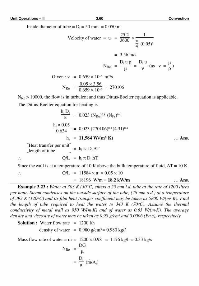
Unit Operations – II 3.60 Convection
Inside diameter of tube = Di = 50 mm = 0.050 m
Velocity of water = u = 25.2
3600 ×
1
π4
(0.05)2
= 3.56 m/s
NRe = Di u ρ
µ =
Di u
ν (as ν =
µ
ρ )
Given : ν = 0.659 × 10⁻⁶ m2/s
NRe = 0.05 × 3.56
0.659 × 10–6 = 270106
NRe > 10000, the flow is in turbulent and thus Dittus-Boelter equation is applicable.
The Dittus-Boelter equation for heating is
hi Di
k = 0.023 (NRe)0.8 (NPr)0.4
hi × 0.05
0.634 = 0.023 (270106)0.8 (4.31)0.4
hi = 11,584 W/(m2·K) … Ans.
Heat transfer per unit
length of tube = hi π Di ∆T
∴ Q/L = hi π Di ∆T
Since the wall is at a temperature of 10 K above the bulk temperature of fluid, ∆T = 10 K.
∴ Q/L = 11584 × π × 0.05 × 10
= 18196 W/m = 18.2 kW/m … Ans.
Example 3.23 : Water at 303 K (30oC) enters a 25 mm i.d. tube at the rate of 1200 litres
per hour. Steam condenses on the outside surface of the tube, (28 mm o.d.) at a temperature
of 393 K (120oC) and its film heat transfer coefficient may be taken as 5800 W/(m2·K). Find
the length of tube required to heat the water to 343 K (70oC). Assume the thermal
conductivity of metal wall as 950 W/(m·K) and of water as 0.63 W/(m·K). The average
density and viscosity of water may be taken as 0.98 g/cm3 and 0.0006 (Pa·s), respectively.
Solution : Water flow rate = 1200 l/h
density of water = 0.980 g/cm3 = 0.980 kg/l
Mass flow rate of water = .
m = 1200 × 0.98 = 1176 kg/h = 0.33 kg/s
NRe = DG
µ
= Di
µ (
.m/Ai)
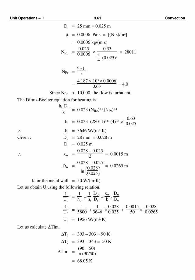
Unit Operations – II 3.61 Convection
Di = 25 mm = 0.025 m
µ = 0.0006 Pa·s = [(N·s)/m2]
= 0.0006 kg/(m·s)
NRe = 0.025
0.0006 ×
0.33
π4
(0.025)2
= 28011
NPr = Cp µ
k
= 4.187 × 103 × 0.0006
0.63 = 4.0
Since NRe > 10,000, the flow is turbulent
The Dittus-Boelter equation for heating is
hi Di
k = 0.023 (NRe)0.8 (NPr)0.4
hi = 0.023 (28011)0.8 (4)0.4 ×
0.63
0.025
∴ hi = 3646 W/(m2·K)
Given : Do = 28 mm = 0.028 m
Di = 0.025 m
∴ xw = 0.028 – 0.025
2 = 0.0015 m
Dw = 0.028 – 0.025
ln
0.028
0.025
= 0.0265 m
k for the metal wall = 50 W/(m·K)
Let us obtain U using the following relation.
1
Uo =
1
ho +
1
hi
Do
Di +
xw
k ·
Do
Dw
1
Uo =
1
5800 +
1
3646 ×
0.028
0.025 +
0.0015
50 ×
0.028
0.0265
Uo = 1956 W/(m2·K)
Let us calculate ∆Tlm.
∆T1 = 393 – 303 = 90 K
∆T2 = 393 – 343 = 50 K
∆Tlm = (90 – 50)
ln (90/50)
= 68.05 K
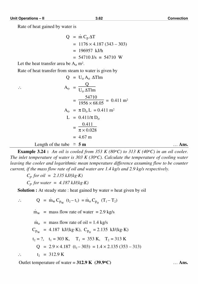
Unit Operations – II 3.62 Convection
Rate of heat gained by water is
Q = .
m Cp ∆T
= 1176 × 4.187 (343 – 303)
= 196957 kJ/h
= 54710 J/s ≡ 54710 W
Let the heat transfer area be Ao m2.
Rate of heat transfer from steam to water is given by
Q = Uo Ao ∆Tlm
∴ Ao = Q
Uo ∆Tlm
= 54710
1956 × 68.05 = 0.411 m2
Ao = π Do L = 0.411 m2
L = 0.411/π Do
= 0.411
π × 0.028
= 4.67 m
Length of the tube ~– 5 m … Ans.
Example 3.24 : An oil is cooled from 353 K (80oC) to 313 K (40oC) in an oil cooler.
The inlet temperature of water is 303 K (30oC). Calculate the temperature of cooling water
leaving the cooler and logarithmic mean temperature difference assuming flow to be counter
current, if the mass flow rate of oil and water are 1.4 kg/s and 2.9 kg/s respectively.
Cp for oil = 2.135 kJ/(kg·K)
Cp for water = 4.187 kJ/(kg·K)
Solution : At steady state : heat gained by water = heat given by oil
∴ Q = .
mw Cpw (t2 – t1) =
.mo Cpo
(T1 – T2)
.
mw = mass flow rate of water = 2.9 kg/s
.
mo = mass flow rate of oil = 1.4 kg/s
Cpw = 4.187 kJ/(kg·K), Cpo
= 2.135 kJ/(kg·K)
t2 = ?, t1 = 303 K, T1 = 353 K, T2 = 313 K
Q = 2.9 × 4.187 (t2 – 303) = 1.4 × 2.135 (353 – 313)
∴ t2 = 312.9 K
Outlet temperature of water = 312.9 K (39.9oC) … Ans.
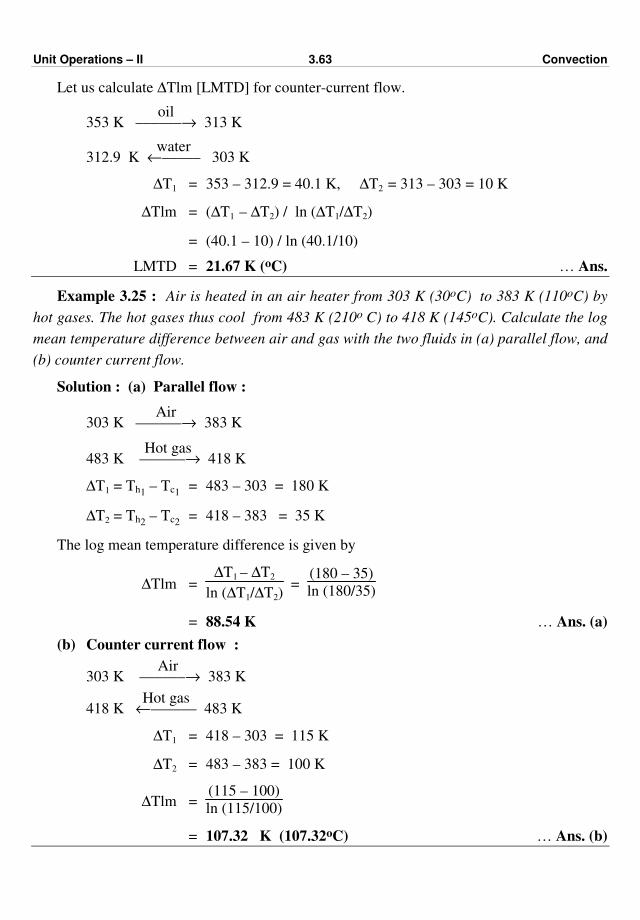
Unit Operations – II 3.63 Convection
Let us calculate ∆Tlm [LMTD] for counter-current flow.
353 K oil
––––––→ 313 K
312.9 K water
←––––– 303 K
∆T1 = 353 – 312.9 = 40.1 K, ∆T2 = 313 – 303 = 10 K
∆Tlm = (∆T1 – ∆T2) / ln (∆T1/∆T2)
= (40.1 – 10) / ln (40.1/10)
LMTD = 21.67 K (oC) … Ans.
Example 3.25 : Air is heated in an air heater from 303 K (30oC) to 383 K (110oC) by
hot gases. The hot gases thus cool from 483 K (210o C) to 418 K (145oC). Calculate the log
mean temperature difference between air and gas with the two fluids in (a) parallel flow, and
(b) counter current flow.
Solution : (a) Parallel flow :
303 K Air
––––––→ 383 K
483 K Hot gas
––––––→ 418 K
∆T1 = Th1 – Tc1 = 483 – 303 = 180 K
∆T2 = Th2 – Tc2 = 418 – 383 = 35 K
The log mean temperature difference is given by
∆Tlm = ∆T1 – ∆T2
ln (∆T1/∆T2) =
(180 – 35)
ln (180/35)
= 88.54 K … Ans. (a)
(b) Counter current flow :
303 K Air
––––––→ 383 K
418 K Hot gas
←–––––– 483 K
∆T1 = 418 – 303 = 115 K
∆T2 = 483 – 383 = 100 K
∆Tlm = (115 – 100)
ln (115/100)
= 107.32 K (107.32oC) … Ans. (b)

Unit Operations – II 3.64 Convection
Example 3.26 : A cooling coil is incorporated in a reaction vessel of which the contents
are kept uniformly at a temperature of 360 K by means of a stirrer. The inlet and outlet
temperatures of the cooling water are 280 K and 320 K respectively. Find out the outlet
temperature of water if the length of cooling coil were increased 5 times the original
assuming that the overall heat transfer coefficient to be constant over the length of the tube
and is independent of water temperature.
Solution : The rate of heat transfer is given by
Q = U A ∆Tlm
I. For initial conditions :
∆T1 = 360 – 280 = 80 K, ∆T2 = 360 – 320 = 40 K
The rate of heat transfer is
Q1 = .
m1 Cp1 (T2 – T1) = U1 A1 ∆Tlm (I)
.
m1 × 4.187 (320 – 280) = U1 A1 [(80 – 40) ln (80/20)]
.
m1 / U1 A1 = 0.345
II. For final conditions :
.
m2 = .
m1, U2 = U1 and A2 = 5 A1 (since it is given that L2 = 5 L1)
Let T be the outlet temperature of water in the final conditions.
Q2 = .
m2 × 4.187 (T – 280) = U2 A2 ∆Tlm (II) = U2 A2
(360 – 280) – (360 – T)
ln
360 – 280
360 – T
∴ Q2 = .
m1 × 4.187 (T – 280) = 5 U1 A1
(360 – 280) – (360 – T)
ln
360 – 280
360 – T
Substituting .
m1/U1A1 = 0.345 in the above equation yields
0.289 (T – 280) = (T – 280) / [ln 80/(360 – T)]
ln [80/(360 – T)] = 3.467
∴ T = outlet temperature of water = 357.5 K … Ans.
Example 3.27 : In an oil cooler, 60 g/s of hot oil enters a thin pipe of diameter of 25 mm.
An equal mass of cooling water flows through the annular space between pipe and large
concentric pipe. The oil and water are flowing in a counter current fashion. Calculate the
outlet temperature of water and area of heat transfer required from the following data :
Inlet temperature of oil = 420 K
Outlet temperature of oil = 320 K
Inlet temperature of water = 290 K
Oil side heat transfer coefficient = 1.6 kW/(m2·K)
Water side heat transfer coefficient = 3.6 kW/(m2·K)
Specific heat of oil = 2.0 kJ/(kg·K)
Specific heat of water = 4.18 kJ/(kg·K)
Metal wall resistance and scale resistance may be neglected.

Unit Operations – II 3.65 Convection
Solution :
Mass flow rate of oil = .
mo = 60 g/s
= 6.0 × 10⁻² kg/s
Rate of heat flow = Heat removed from oil = Q
= .
mo Cpo (T1 – T2)
= 6.0 × 10–2 × 2.0 × (420 – 320)
= 12 kJ/s
= 12 kW
Let us find the outlet temperature of water.
Given : .
mw = .
mo = 6.0 × 10⁻² kg/s
t1 = inlet temperature of water = 290 K, Cpw = 4.18 kJ/(kg·K)
A heat balance yields
Heat removed from oil = Heat gained by water
Q = .
mw Cpw (t2 – t1)
12 = 6.0 × 10–2 × 4.18 × (t2 – 290)
t2 = 338 K
Outlet temperature of water = 338 K … Ans.
Logarithmic mean temperature difference for the counter current flow is :
∆T1 = T1 – t2 = 420 – 338 = 82 K
∆T2 = T2 – t1 = 320 – 290 = 30 K
∆Tlm = 82 – 30
ln (82/30) = 51.7 K
Overall heat transfer coefficient is given by
1
U =
1
ho +
1
hi
= 1
1.6 +
1
3.6 = 1.108 kW/(m2·K) = 1108 W/(m2·K)
Let us calculate A. The rate of heat transfer is given by
Q = UA ∆Tlm
where Q = 12 kW = 12000 W, U = 1108 W/(m2⋅K) and ∆Tlm = 51.7 K

Unit Operations – II 3.66 Convection
∴ A = Q
U · ∆Tlm
A = 12000
1108 × 51.7
= 0.210 m2 … Ans.
Given : Do = 25 mm = 0.025 m
Let us find the length of tube, i.e., the length of heat transfer.
A = π Do L
L = A/π Do = 0.210 / (π × 0.025)
= 2.67 m … Ans.
Example 3.28 : Determine the heating surface of an economiser in which a primary
(hot gases) and a secondary fluid (water) are in counter current flow using the following
data :
Mass flow rate of gas = 1.22 kg/s
Specific heat of gas = 1.045 kJ/(kg·K)
Inlet temperature of gas = 693 K (420 oC)
Mass flow rate of water = 0.67 kg/s
Inlet temperature of water = 378 K (105 oC)
Rate of heat transfer from hot gas to water = 270 kW
Heat transfer coefficient from gases to water (i.e. U) = 80 W/(m2·K)
Solution : Let us find the outlet temperature of water.
Given : Q = 270 kW = 270 × 103 W = 270 kJ/s
For water : Rate of heat gained by water = Q = .
mw Cpw (t2 – t1)
∴ 270 = 0.67 × 4.187 (t2 – 378)
t2 = outlet temperature of water = 474 K
Let us find the outlet temperature of the hot gases.
For hot gas : The rate of heat removal from the hot gases is
Q = .
mh Cph (T1 – T2)
270 = 1.22 × 1.045 (693 – T2)
T2 = outlet temperature of the hot gases = 481.2 K
Let us find ∆Tlm (LMTD) for counter current flow.
693 K Hot gas–––––→ 481.2 K
474 K Water
←––––– 378 K
∆T1 = 693 – 474 = 219 K, ∆T2 = 481.2 – 378 = 103.2 K
∆Tlm = (219 – 103.2) / ln (219/103.2) = 153.9 K

Unit Operations – II 3.67 Convection
The rate of heat transfer is given by
Q = U A ∆Tlm
∴ A = Q/(U · ∆Tlm) = 270 × 103
80 × 153.9 = 21.93 m2
Heating surface of the economiser = 21.93 m2. … Ans.
Example 3.29 : Water is to be heated from 298 K (25oC) to 313 K (40oC) at a rate of
30 kg/s. Hot water is available at 353 K (80oC) at a rate of 24 kg/s for heating in a counter
current exchanger. Calculate the heat transfer area required, if the overall heat transfer
coefficient is 1220 W/(m2·K).
Solution : At steady state : Heat gained by cold water = Heat removed from hot water
∴ Q = .
mc Cpc (t2 – t1) =
.mh Cph
(T1 – T2)
.
mc = mass flow rate of cold water = 30 kg/s
.
mh = mass flow rate of hot water = 24 kg/s
Cpc = Cph
= 4.187 kJ/(kg·K)
t2 = 313 K, t1 = 298 K, T1 = 353 K, T2 = ?
Q = 30 × 4.187 × (313 – 298) = 1884.15 kJ/s
= 1884.15 × 103 J/s ≡ 1884.15 × 103 W
Q = Heat gained by cold water = Heat lost by hot water
1884.15 = 24 × 4.187 (353 – T2)
T2 = 334.2 K
The rate of heat transfer is given by
298 K Cold water
––––––––→ 313 K
334.2 K Hot water←–––––– 353 K
∆T1 = 353 – 313 = 40 K, ∆T2 = 334.2 – 298 = 36.2 K
∆Tlm for counter current flow = (40 – 36.2) / ln (40/36.2) = 38.1 K
The rate of heat transfer is given by
Q = U A ∆Tlm
A = Q/U · ∆Tlm = 1884.15 × 103
1220 × 38.1
= 40.53 m2
Heat transfer area required = 40.53 m2 … Ans.
Example 3.30 : Evaluate the inside heat transfer coefficient. Heavy oil flows at a rate of
0.5 kg/s through a tube of 19 mm inside diameter and is heated from 311 to 327 K by
condensing steam at 373 K.

Unit Operations – II 3.68 Convection
Data : Properties of oil at 319 K (mean/average oil temperature)
k for oil = 0.14 W/(m·K)
Cp for oil = 2.1 kJ/(kg·K)
µ for oil = 154 (mN·s)/m2
µ at mean wall temperature (346 K) = 87.0 (mN·s)/m2
Length of tube = 1.5 m
Solution : Mass flow rate of oil = .
m = 0.5 kg/s
Diameter of tube = 19 mm = 0.019 m
Mean temperature of oil = (311 + 327)/2 = 319 K
µ of oil at 319 K = 154 (mN·s)/m2
= 154 × 10–3 (N·s)/m2 [i.e. kg/(m·s)]
Cross sectional area of tube = π/4 × (0.019)2 = 2.835 × 10⁻⁴ m2
G = mass velocity = .
m /A = 0.5 / 2.835 × 10–4 = 1763.67 kg/(m2·s)
Let us calculate NRe.
NRe = Duρ
µ =
DG
µ =
0.019 × 1763.67
154 × 10–3 = 217.6
As NRe is less than 2100, the flow is laminar.
The Sieder-Tate equation for laminar flow is
hi Di
k = 2.0
.
m Cp
k L
1/3
µ
µw
0.14
where .
m = 0.5 kg/s, L = 1.5 m, k = 0.14 W/(m·K)
µ = 154 × 10–3 kg/(m·s)
µw = viscosity at the mean wall temperature [(373 + 319)/2] i.e. at 346 K
µw = 87 (mN·s)/m2 = 87 × 10–3 (N·s)/m2 = 87 × 10–3 kg/(m·s)
Cp = 2.1 kJ/(kg·K) = 2.1 × 10³ J/(kg·K)
hi × 0.019
0.14 = 2
0.5 × 2.1 × 103
0.14 × 1.5
1/3
154 × 10–3
87 × 10–3
0.14
∴ hi = 265.33 W/(m2·K)
Inside heat transfer coefficient = 265.33 W/(m2·K) … Ans.

Unit Operations – II 3.69 Convection
Example 3.31 : Pure iso-butane vapours are to be condensed at 331.7 K in a horizontal
tubular heat exchanger using water as a cooling medium. Determine the inside film heat
transfer coefficient based on the outside diameter of tube.
Outside diameter of tube = 19 mm
Wall thickness of tube = 1.6 mm
Inlet temperature of water = 301 K
Outlet temperature of water = 315 K
Water flow rate through each tube = 0.217 kg/s
Solution :
Water flow rate = ⋅
m = 0.217 kg/s
i.d. of tube = (19.0 – 2 × 1.6) = 15.7 mm = 0.0157 m
Cross sectional area for flow = Ai = π/4 × (0.0157)2 = 0.000194 m2
Water velocity through tube = u = .
m /ρ · Ai
= 0.217
1000 × 0.000194 = 1.12 m/s
Average temperature of water = T = (T1 + T2)/2 = (301 + 315)/2 = 308 K
The inside heat transfer coefficient (for water) may be calculated by
hi = 1063 (1 + 0.00293 × T) u0.8 / (di)0.20
= 1063 (1 + 0.00293 × 308) (1.12)0.8 / (0.0157)0.20
= 5084 W/(m2·K)
Inside heat transfer coefficient based on the outside diameter (hio) is calculated as
hio = hi
Di
Do = 5084 ×
0.0157
0.019
= 4201 W/(m2·K)
= 4.20 kW/(m2 ·K) … Ans.
Example 3.32 : A heat exchanger is required to cool 20 kg/s of hot water from 360 K to
335 K by means of cold water flowing at 25 kg/s. Inlet temperature of cold water is 300 K.
Overall heat transfer coefficient is 2 kW/(m2·K). Calculate the area of heat transfer required
in (a) a counter current flow heat exchanger and (b) in a 1–2 pass heat exchanger (cold
water flowing twice through heat exchanger).
Data : Specific heat of cold and hot water may be taken as 4.187 kJ/(kg·K)
and LMTD correction factor = 0.94
Solution : The heat load of the exchanger is the heat to be removed from water and is
given by
Q = .
m1 Cp1 (T1 – T2)

Unit Operations – II 3.70 Convection
where .
m1 = 20 kg/s, Cp1 = 4.187 kJ/(kg·K)
T1 = 360 K, T2 = 335 K
Q = 20 × 4.187 × (360 – 335)
Q = 2093.5 kJ/s = 2093.5 kW … heat given out by hot water.
For cold water :
t1 = inlet temperature of cold water = 300 K
.
m2 = mass flow rate of cold water = 25 kg/s
t2 = outlet temperature of cold water
At steady state, heat given out by the hot water is equal to heat gained by the cold water.
Therefore, Q = .
m2 Cp2 (t2 – t1)
2093.5 = 25 × 4.187 (t2 – 300)
Solving for t2 gives
t2 = 320 K
I. Case (a) : Counter-current flow heat exchanger
360 K Hot water––––––→ 335 K
320 K Cold water←––––––– 300 K
∆T1 = T1 – t2 = 360 – 320 = 40 K
∆T2 = T2 – t1 = 335 – 300 = 35 K
∆Tlm for counter current flow = (∆T1 – ∆T2)
ln (∆T1/∆T2)
∆Tlm = (40 – 35) / ln (40/35) = 37.4 K
Let us calculate the heat transfer area.
The rate of heat transfer is given by
Q = U A ∆Tlm
A = Q/U ∆Tlm
where Q = 2090 kW = 2090 × 103 W
U = 2.0 kW/(m2·K) = 2 × 10³ W/(m2·K)
∴ A = 2090 × 103
2.0 × 103 × 37.4
= 27.94 m2 … Ans. (a)
II. Case (b) : 1-2 pass heat exchanger.
∆Tlm = 37.4 K
LMTD correction factor = FT = 0.94
The rate of heat transfer in this case is given by
Q = U A FT ∆Tlm
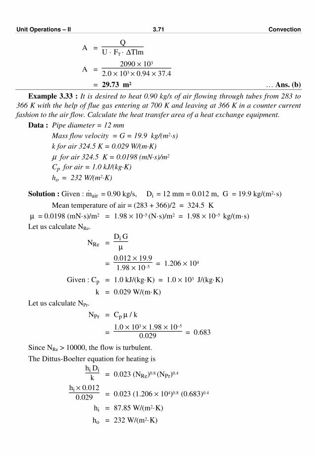
Unit Operations – II 3.71 Convection
A = Q
U · FT · ∆Tlm
A = 2090 × 103
2.0 × 103 × 0.94 × 37.4
= 29.73 m2 … Ans. (b)
Example 3.33 : It is desired to heat 0.90 kg/s of air flowing through tubes from 283 to
366 K with the help of flue gas entering at 700 K and leaving at 366 K in a counter current
fashion to the air flow. Calculate the heat transfer area of a heat exchange equipment.
Data : Pipe diameter = 12 mm
Mass flow velocity = G = 19.9 kg/(m2·s)
k for air 324.5 K = 0.029 W/(m·K)
µ for air 324.5 K = 0.0198 (mN·s)/m2
Cp for air = 1.0 kJ/(kg·K)
ho = 232 W/(m2·K)
Solution : Given : .
mair = 0.90 kg/s, Di = 12 mm = 0.012 m, G = 19.9 kg/(m2·s)
Mean temperature of air = (283 + 366)/2 = 324.5 K
µ = 0.0198 (mN·s)/m2 = 1.98 × 10⁻⁵ (N·s)/m2 = 1.98 × 10⁻⁵ kg/(m·s)
Let us calculate NRe.
NRe = Di G
µ
= 0.012 × 19.9
1.98 × 10–5 = 1.206 × 10⁴
Given : Cp = 1.0 kJ/(kg·K) = 1.0 × 10³ J/(kg·K)
k = 0.029 W/(m·K)
Let us calculate NPr.
NPr = Cp µ / k
= 1.0 × 103 × 1.98 × 10–5
0.029 = 0.683
Since NRe > 10000, the flow is turbulent.
The Dittus-Boelter equation for heating is
hi Di
k = 0.023 (NRe)0.8 (NPr)0.4
hi × 0.012
0.029 = 0.023 (1.206 × 10⁴)0.8 (0.683)0.4
hi = 87.85 W/(m2·K)
ho = 232 W/(m2·K)

Unit Operations – II 3.72 Convection
The overall heat transfer coefficient is given by
1
U =
1
hi +
1
ho
= 1
87.85 +
1
232 = 0.0114 + 0.0043 = 0.0157
U = 63.7 W/(m2·K)
The rate of heat addition to air is given by
Q = (.
m × Cp)air (t2 – t1)
Q = 0.9 × 1.0 × (366 – 283) = 74.7 kJ/s
= 74.7 × 10³ J/s ≡ 74.7 × 10³ W
Let us calculate LMTD for counter current flow.
283 K Air
––––––→ 366 K
366 K Flue gas
←–––––– 700 K
∆T1 = T1 – t2 = 700 – 366 = 334 K
∆T2 = T2 – t1 = 366 – 283 = 83 K
∆Tlm = (∆T1 – ∆T2)
ln (∆T1/∆T2)
= (334 – 83)
ln (334/83) = 180 K
Let us calculate the heat transfer area. The rate of heat transfer is given by
Q = U A ∆Tlm
A = Q/U · ∆Tlm
= 74.7 × 10³ / (63.7 × 180)
= 6.52 m2 … Ans.
Example 3.34 : A light motor oil is to be heated from 338.5 K (65.5oC) to
394.1 K (121.1oC). The pipe wall is at 449.7 K (176.7oC). The light motor oil flows through
a 10 mm pipe, 5 m long at a rate of 41 kg/h. Calculate the heat transfer coefficient using the
following data :
Data : Properties of oil at the average bulk temperature are :
Cp = 2.01 kJ/(kg·K), k = 0.142 W/(m·K)
µ = 4.65 × 10⁻³ kg/(m·s)
Viscosity of oil at the wall temperature = µw = 1.37 × 10⁻³ kg/(m·s)
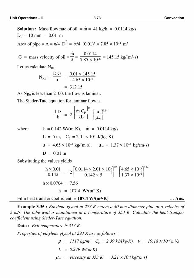
Unit Operations – II 3.73 Convection
Solution : Mass flow rate of oil = ⋅
m = 41 kg/h = 0.0114 kg/s
Di = 10 mm = 0.01 m
Area of pipe = A = π/4 D2
i = π/4 (0.01)2 = 7.85 × 10⁻⁵ m2
G = mass velocity of oil =
⋅m
a =
0.0114
7.85 × 10–6 = 145.15 kg/(m2·s)
Let us calculate NRe.
NRe = DiG
µ =
0.01 × 145.15
4.65 × 10–3
= 312.15
As NRe is less than 2100, the flow is laminar.
The Sieder-Tate equation for laminar flow is
hD
k = 2
.
m Cp
kL
1/3
µ
µw
0.14
where k = 0.142 W/(m·K), .
m = 0.0114 kg/s
L = 5 m, Cp = 2.01 × 10³ J/(kg·K)
µ = 4.65 × 10⁻³ kg/(m·s), µw = 1.37 × 10⁻³ kg/(m·s)
D = 0.01 m
Substituting the values yields
h × 0.01
0.142 = 2
0.0114 × 2.01 × 103
0.142 × 5
1/3
4.65 × 10⁻³
1.37 × 10⁻³
0.14
h × 0.0704 = 7.56
h = 107.4 W/(m2·K)
Film heat transfer coefficient = 107.4 W/(m2·K) … Ans.
Example 3.35 : Ethylene glycol at 273 K enters a 40 mm diameter pipe at a velocity of
5 m/s. The tube wall is maintained at a temperature of 353 K. Calculate the heat transfer
coefficient using Sieder-Tate equation.
Data : Exit temperature is 313 K.
Properties of ethylene glycol at 293 K are as follows :
ρ = 1117 kg/m3, Cp = 2.39 kJ/(kg·K), ν = 19.18 × 10⁻⁶ m2/s
k = 0.249 W/(m·K)
µw = viscosity at 353 K = 3.21 × 10⁻³ kg/(m·s)
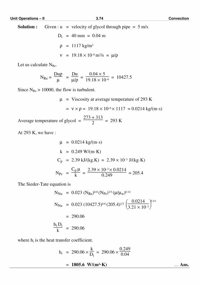
Unit Operations – II 3.74 Convection
Solution : Given : u = velocity of glycol through pipe = 5 m/s
Di = 40 mm = 0.04 m
ρ = 1117 kg/m3
ν = 19.18 × 10⁻⁶ m2/s = µ/ρ
Let us calculate NRe.
NRe = Duρ
µ =
Du
µ/ρ =
0.04 × 5
19.18 × 10–6 = 10427.5
Since NRe > 10000, the flow is turbulent.
µ = Viscosity at average temperature of 293 K
= ν × ρ = 19.18 × 10–6 × 1117 = 0.0214 kg/(m·s)
Average temperature of glycol = 273 + 313
2 = 293 K
At 293 K, we have :
µ = 0.0214 kg/(m·s)
k = 0.249 W/(m·K)
Cp = 2.39 kJ/(kg.K) = 2.39 × 10⁻³ J/(kg·K)
NPr = Cp µ
k =
2.39 × 10–3 × 0.0214
0.249 = 205.4
The Sieder-Tate equation is
NNu = 0.023 (NRe)0.8 (NPr)1/3 (µ/µw)0.14
NNu = 0.023 (10427.5)0.8 (205.4)1/3
0.0214
3.21 × 10⁻³
0.14
= 290.06
hi Di
k = 290.06
where hi is the heat transfer coefficient.
hi = 290.06 × k
Di = 290.06 ×
0.249
0.04
= 1805.6 W/(m2·K) … Ans.
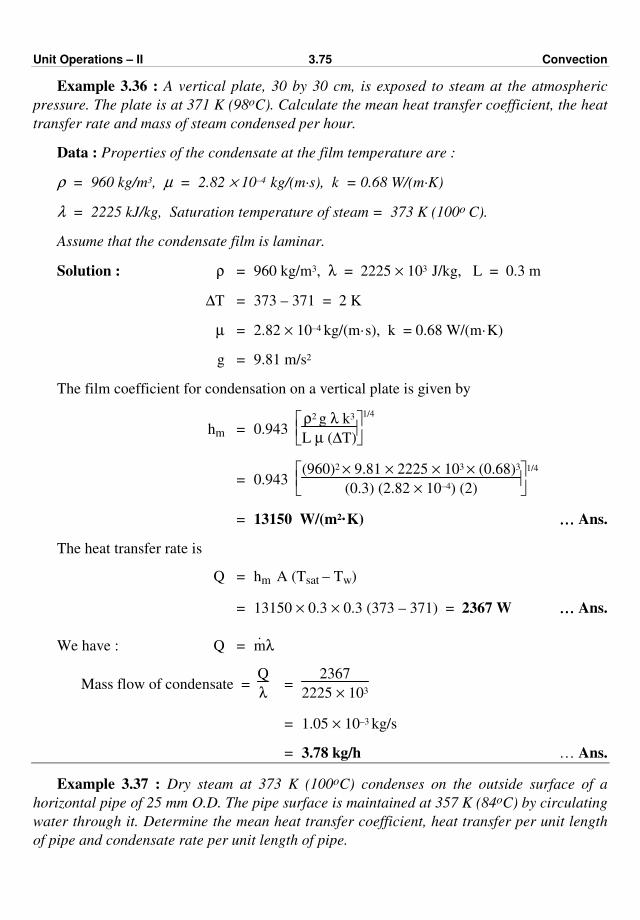
Unit Operations – II 3.75 Convection
Example 3.36 : A vertical plate, 30 by 30 cm, is exposed to steam at the atmospheric
pressure. The plate is at 371 K (98oC). Calculate the mean heat transfer coefficient, the heat
transfer rate and mass of steam condensed per hour.
Data : Properties of the condensate at the film temperature are :
ρ = 960 kg/m3, µ = 2.82 × 10⁻⁴ kg/(m·s), k = 0.68 W/(m·K)
λ = 2225 kJ/kg, Saturation temperature of steam = 373 K (100o C).
Assume that the condensate film is laminar.
Solution : ρ = 960 kg/m3, λ = 2225 × 103 J/kg, L = 0.3 m
∆T = 373 – 371 = 2 K
µ = 2.82 × 10⁻⁴ kg/(m·s), k = 0.68 W/(m·K)
g = 9.81 m/s2
The film coefficient for condensation on a vertical plate is given by
hm = 0.943
ρ2 g λ k3
L µ (∆T)
1/4
= 0.943
(960)2 × 9.81 × 2225 × 103 × (0.68)3
(0.3) (2.82 × 10⁻⁴) (2)
1/4
= 13150 W/(m2·K) ………… Ans.
The heat transfer rate is
Q = hm A (Tsat – Tw)
= 13150 × 0.3 × 0.3 (373 – 371) = 2367 W ………… Ans.
We have : Q = ⋅
mλ
Mass flow of condensate = Q
λ =
2367
2225 × 103
= 1.05 × 10⁻³ kg/s
= 3.78 kg/h … Ans.
Example 3.37 : Dry steam at 373 K (100oC) condenses on the outside surface of a
horizontal pipe of 25 mm O.D. The pipe surface is maintained at 357 K (84oC) by circulating
water through it. Determine the mean heat transfer coefficient, heat transfer per unit length
of pipe and condensate rate per unit length of pipe.
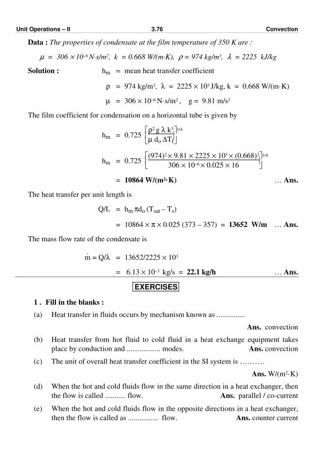
Unit Operations – II 3.76 Convection
Data : The properties of condensate at the film temperature of 350 K are :
µ = 306 × 10–6 N·s/m2, k = 0.668 W/(m·K), ρ = 974 kg/m3, λ = 2225 kJ/kg
Solution : hm = mean heat transfer coefficient
ρ = 974 kg/m3, λ = 2225 × 103 J/kg, k = 0.668 W/(m·K)
µ = 306 × 10–6 N·s/m2 , g = 9.81 m/s2
The film coefficient for condensation on a horizontal tube is given by
hm = 0.725
ρ2 g λ k3
µ do ∆Tf
1/4
hm = 0.725
(974)2 × 9.81 × 2225 × 103 × (0.668)3
306 × 10–6 × 0.025 × 16
1/4
= 10864 W/(m2·K) … Ans.
The heat transfer per unit length is
Q/L = hm πdo (Tsat – Ts)
= 10864 × π × 0.025 (373 – 357) = 13652 W/m … Ans.
The mass flow rate of the condensate is
⋅
m = Q/λ = 13652/2225 × 103
= 6.13 × 10⁻³ kg/s = 22.1 kg/h … Ans.
EXERCISES
1 . Fill in the blanks :
(a) Heat transfer in fluids occurs by mechanism known as ...............
Ans. convection
(b) Heat transfer from hot fluid to cold fluid in a heat exchange equipment takes
place by conduction and .................. modes. Ans. convection
(c) The unit of overall heat transfer coefficient in the SI system is ……….
Ans. W/(m2·K)
(d) When the hot and cold fluids flow in the same direction in a heat exchanger, then
the flow is called ........... flow. Ans. parallel / co-current
(e) When the hot and cold fluids flow in the opposite directions in a heat exchanger,
then the flow is called as ................ flow. Ans. counter current
Unit Operations – II 3.77 Convection
(f) Film heat transfer coefficients are higher for .......... condensation than for
filmwise condensation. Ans. dropwise
(g) In case of ........ boiling, vaporisation takes place directly from the surface.
Ans. nucleate
(h) The SI unit of film heat transfer coefficient is .......... Ans. W/(m2·K)
(i) The dirt factor / fouling factor has the units ........ in SI system. Ans. (m2·K)/W
(j) The ratio of Cp · µ to k is known as ....... number. Ans. Nusselt
(k) Thermal resistance in case of convection heat transfer has the units of ..........
Ans. (m2·K)/W
(l) In forced convection, the effect of liquid viscosity (for viscous liquids) is taken
into account in case of .......... equation. Ans. Sieder-Tate
2. Give the Dittus-Boelter equation for turbulent flow for heating.
3. Give the Dittus-Boelter equation for turbulent flow for cooling.
4. Give the Sieder-Tate equation used to calculate the film coefficient in case of
laminar flow.
5. Give the Sieder-Tate equation used to calculate the film coefficient in case of
turbulent flow.
6. What do you mean by film heat transfer coefficient ?
7. For a double pipe heat exchanger, give its equivalent diameter in terms of D1 and
D2, where D1 is the outside diameter of the inside pipe and D2 is the inside
diameter of the outside pipe.
8. What do you mean by natural convection ? Give example of heat transfer by
natural convection.
9. Define forced convection and give its example.
10. Compare natural convection with forced convection (Three points).
11. Compare parallel flow with counter current flow in heat exchangers (Three
points).
12. Define drop-wise condensation.
13. Compare drop-wise condensation with film-wise condensation (Three points).
14. Define co-current and counter current flow with neat sketches.
15. State the relationship between overall heat transfer coefficient and individual heat
transfer coefficients.
16. Write the relationship between U and hi, ho, xw/k and Rd.
17. Explain in brief heat transfer to boiling liquids.
18. Derive the relationship Q = UA ∆Tlm.
Unit Operations – II 3.78 Convection
19. Write in brief on dirt factor / fouling factor with respect to heat transfer.
20. State various resistances in series when heat flows from one fluid to another
through a solid wall in a heat exchange equipment.
(Ans. Resistances are : hot fluid film resistance, solid wall resistance, cold fluid
film resistance and dirt or fouling resistances.)
21. State different types of flow arrangements in heat exchanger.
22. What do you mean by counter current heat exchanger and cross flow heat
exchanger ?
23. Define the terms nucleate boiling and film boiling.
24. Give the physical significance of
(1) Reynolds number (2) Nusselt number and (3) Prandtl number.
ppp
(4.1)
CHAPTER FOUR
RADIATION
Heat transfer by radiation usually takes place simultaneously with heat transfer by
convection and conduction. The heat transfer by radiation is of much more importance at
high temperature levels as compared to the other two mechanisms. Direct fired kettles,
electric heaters, steam boilers, rotary kiln, etc. are the examples of chemical process
equipments where radiation is a major energy transfer mechanism.
Radiation : It refers to the transport of energy through space by electromagnetic waves.
It depends upon the electromagnetic waves as a means for transfer of energy from a
source to a receiver.
Radiant energy is of the same nature as the ordinary visible light. It travels in the straight
lines and it may be reflected from a surface. The electromagnetic waves with wavelength
ranging from 0.50 to 50 µm (microns, 1 µm = 10–6 m) are of importance to radiant-heat
transfer. Radiation of a single wavelength is called as monochromatic. Thermal radiation is
the energy emitted by a body due to its temperature and we restrict our discussion to this type
of radiation.
Typical examples of heat transfer by radiation :
(i) Transfer of heat from the sun to the earth.
(ii) Heat loss from an unlagged steam pipe.
(iii) Use of energy from the sun in solar heaters.
(iv) Heating of a cold room by a radiant electric heater.
In constrast to heat transfer by conduction and convection, radiation heat transfer does
not require an intervening medium (material or liquid) between two locations and the heat
can be transmitted by radiation mode across an absolute vacuum.
Radiation is the only significant mode of energy/heat transfer when no medium is
present (e.g., the heat leakage through the evacuated walls of a thermos flask).
Absorptivity, Reflectivity and Transmissivity : Any substance receives and gives off/emits energy in the form of electromagnetic waves.
When energy emitted by a heated body falls on a second body (i.e., thermal radiation falling
on a body), it will be partly absorbed, partly reflected back and partly transmitted through the
body. It is only the absorbed energy that appears as a heat in the body.
[incident radiation = heat absorbed + heat transmitted + heat reflected]
The proportions of the incident energy that are absorbed, reflected and transmitted
depend mainly on the characteristics of a receiver (Incident radiation = heat absorbed + heat
transmitted + heat reflected).
The fraction of the incident radiation on a body that is absorbed by the body is known as
the absorptivity and may be denoted by the letter 'a'.

Unit Operations – II 4.2 Radiation
The fraction of the incident radiation on a body that is reflected by the body is known as
the reflectivity and may be denoted by the letter 'r'.
Transmitted
Reflected Incident
Absorbed
Fig. 4.1 : Reflection, absorption and transmission of radiation
The fraction of the incident radiation on a body that is transmitted through the body is
known as the transmissivity and may be denoted by the letter 'ττττ'. The energy balance about
a body (a receiver) on which the total incident energy falling is unity (i.e., the sum of these
fractions is unity) is given as :
a + r + τ = 1.0 … (4.1)
A majority of engineering materials are opaque (i.e., for which the amount transmitted is
very negligible, τ = 0) and in such cases Equation (4.1) simplifies to :
a + r = 1.0 … for an opaque material/surface … (4.2)
If τ = 1, a = r = 0, then all the incident energy passes through the body and it is called
perfectly transparent, e.g., rock salt (NaCl), quartz and fluorite.
If r = 1, a = τ = 0, then all the incident energy is supposed to be entirely reflected by the
body and is specular. If a = 0, r + τ = 1, then the body is called as a white body (non-
absorbing), e.g., a piece of white chalk (white body).
(i) r = 0 represents a nonreflecting surface.
(ii) a = 1 represents a perfectly absorbing surface or a black surface.
(iii) τ = 1 represents a perfectly transparent surface.
(iv) r = 1 represents a perfect reflector.
Black Body :
A body for which a = 1, r = τ = 0, i.e., which absorbs all the incident radiant energy, is
called a black body. It neither reflects nor transmits but absorbs all the radiation incident on
it, so it is treated as an ideal radiation receiver. It is not necessary that the surface of the body
be black in colour. The black body radiates maximum possible amount of energy at a given
temperature and though perfectly black bodies do not exist in nature, some materials may
approach it. Lampblack is the nearest to a black body which absorbs 96 % of the visible light.
The concept of a black body is an idealisation with which the radiation characteristics of
real bodies are compared.
Both the absorptivity and emissivity of perfectly black body are unity.
Unit Operations – II 4.3 Radiation
Laws of Black Body Radiation :
Kirchhoff's Law :
This law sets up a relationship between the emissive power of a body/surface to its
absorptivity.
Consider that two bodies are kept into a furnace held at constant temperature of T K.
Assume that, of the two bodies one is a black body and the other is a non-black body, i.e., the
body having 'a' value less than one. Both the bodies will ultimately attain the temperature of
T K and the bodies neither become hotter nor cooler than the furnace. At this condition of
thermal equilibrium, each body absorbs and emits thermal radiation at the same rate. The
rate of absorption and emission for the black body will be different from that of the non-
black body.
Let the area of non-black body and black body be A1 and A2 respectively. Let 'I' be the
rate at which radiation falling on the bodies per unit area and E1 and Eb be the emissive
powers (emissive power is the total quantity of radiant energy emitted by a body per
unit area per unit time) of the non-black and black body respectively.
At thermal equilibrium, the absorption and emission rates are equal. Therefore,
Ia1 A1 = A1 E1 … (4.3)
∴ Ia1 = E1 … (4.4)
and Iab A2 = A2 Eb … (4.5)
Iab = Eb … (4.6)
From Equations (4.4) and (4.6), we get
E1
a1 =
Eb
ab … (4.7)
where a1, ab are the absorptivities of the non-black and black bodies, respectively.
If we introduce a second body (non-black) then for the second non-black body, we have
I A3 a2 = E2 A3 … (4.8)
Ia2 = E2 … (4.9)
where a2 and E2 are the absorptivity and emissive power of the second non-black body.
Combining Equations (4.4), (4.6) and (4.9), we get
E1
a1 =
E2
a2 =
Eb
ab = Eb … (4.10)
(As the absorptivity of the black body is 1.0)
Statement of Kirchhoff's law
It states that, at thermal equilibrium the ratio of the total emissive power to its
absorptivity is the same for all bodies. Equation (4.10) is the mathematical statement of
Kirchhoff's law.
Unit Operations – II 4.4 Radiation
The emissivity 'e' of any body is defined as the ratio of the total emissive power E of
the body to that of a black body Eb at the same temperature. The emissivity depends on
the temperature of the body only. The emissivity of a body is a measure of how it emits
radiant energy in comparison with a black body at the same temperature.
e = E
Eb … (4.11)
Since E
a is constant for all bodies
E
a =
Eb
ab … (4.12)
e = E
Eb =
a
ab … (4.13)
but ab = 1 (for black body)
∴ e = a … (4.14)
Thus, when any body is in thermal equilibrium with its surroundings, its emissivity and
absorptivity are equal. Equation (4.14) may be taken as the another statement of Kirchhoff's
law.
Monochromatic emissive power : It is the radiant energy emitted from a body per unit
area per unit time per unit wavelength about the wavelength λ. It is denoted by Eλ. It has the
units of W/(m2·µm).
Total emissive power : It is the total quantity of radiant energy of all wavelength
emitted by a body per unit area per unit time. It is denoted by the symbol E. It has the units of
W/m2 .
For the entire spectrum of radiation from a surface, it is the sum of all the
monochromatic radiations from the surface.
E = ⌡⌠0
∞
Eλ dλ … (4.15)
Monochromatic emissivity : It is the ratio of the monochromatic emissive power of a
body to that of a black body at the same wavelength and temperature.
eλ = Eλ
Eb‚ λ … (4.16)
Gray body :
A body having the same value of the monochromatic emissivity at all wavelengths is
called a gray body.
A gray body is the one of which emissivity is independent of wavelength.
[The word monochromatic indicates that the quantity being defined for a particular
wavelength / single wavelength. Monochromatic property refers to a single wavelength and
total property is the sum of monchromatic values of property. Monochromatic values are not
important to the direct solution of engineering problems.]
Unit Operations – II 4.5 Radiation
Laws of black body radiation :
Steafan-Boltzmann law : It states that the total energy emitted per unit area per unit time
by a black body is directly proportional to the fourth power of its absolute temperature.
Eb ∝ T4 … (4.17)
Eb = σ · T4
where T = Temperature in K
σ = Steafan-Boltzmann constant
= 5.67 × 10⁻⁸ W/(m2·K4)
For a non-black body,
E
Eb = e … (4.18)
E = e · Eb … (4.19)
Combining Equations (4.17) and (4.19), we get
E = e · σ · T4 … (4.20)
where 'e' is the emissivity of the non-black body.
The Steafan-Boltzmann equation is a fundamental relation for all the radiant energy
transfer calculations.
Planck's law :
This law gives a relationship between the monochromatic emissive power of a black
body, absolute temperature and the corresponding wavelength.
Eb‚ λ = 2π hc2 λ–5
ehc/kλT – 1 … (4.21)
where Eb‚ λ is the monochromatic emissive power of the black body / black surface,
W/(m2·µm), h is the Planck's constant, k is the Boltzmann constant, c is the speed of light,
T is the absolute temperature and λ is the wavelength of radiation.
Equation (4.21) can be written as
Eb, λ = C1 λ–5
( )eC2/λT – 1 … (4.22)
where C1 and C2 are constants.
C1 = 3.472 × 10⁻¹⁶ W·m2 and C2 = 0.01439 m·K
Wiens displacement law :
It states that the wavelength at which the maximum monochromatic emissive power is
obtained (i.e., λmax) is inversely proportional to the absolute temperature, or
T λmax = C … (4.23)
when λmax is in micrometers and T is in Kelvins, the value of constant C is equal to 2890.
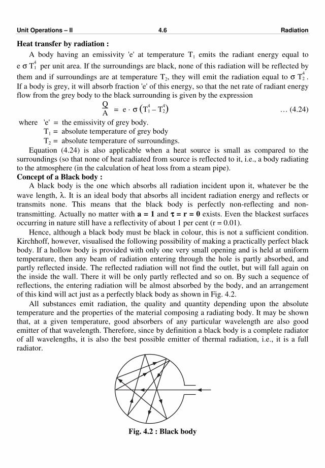
Unit Operations – II 4.6 Radiation
Heat transfer by radiation :
A body having an emissivity 'e' at temperature T1 emits the radiant energy equal to
e σ T4
1 per unit area. If the surroundings are black, none of this radiation will be reflected by
them and if surroundings are at temperature T2, they will emit the radiation equal to σ T4
2 .
If a body is grey, it will absorb fraction 'e' of this energy, so that the net rate of radiant energy
flow from the grey body to the black surrounding is given by the expression
Q
A = e · σ ( )T
4
1 – T4
2 … (4.24)
where 'e' = the emissivity of grey body.
T1 = absolute temperature of grey body
T2 = absolute temperature of surroundings.
Equation (4.24) is also applicable when a heat source is small as compared to the
surroundings (so that none of heat radiated from source is reflected to it, i.e., a body radiating
to the atmosphere (in the calculation of heat loss from a steam pipe).
Concept of a Black body : A black body is the one which absorbs all radiation incident upon it, whatever be the
wave length, λ. It is an ideal body that absorbs all incident radiation energy and reflects or
transmits none. This means that the black body is perfectly non-reflecting and non-
transmitting. Actually no matter with a = 1 and ττττ = r = 0 exists. Even the blackest surfaces
occurring in nature still have a reflectivity of about 1 per cent (r = 0.01).
Hence, although a black body must be black in colour, this is not a sufficient condition.
Kirchhoff, however, visualised the following possibility of making a practically perfect black
body. If a hollow body is provided with only one very small opening and is held at uniform
temperature, then any beam of radiation entering through the hole is partly absorbed, and
partly reflected inside. The reflected radiation will not find the outlet, but will fall again on
the inside the wall. There it will be only partly reflected and so on. By such a sequence of
reflections, the entering radiation will be almost absorbed by the body, and an arrangement
of this kind will act just as a perfectly black body as shown in Fig. 4.2.
All substances emit radiation, the quality and quantity depending upon the absolute
temperature and the properties of the material composing a radiating body. It may be shown
that, at a given temperature, good absorbers of any particular wavelength are also good
emitter of that wavelength. Therefore, since by definition a black body is a complete radiator
of all wavelengths, it is also the best possible emitter of thermal radiation, i.e., it is a full
radiator.
Fig. 4.2 : Black body
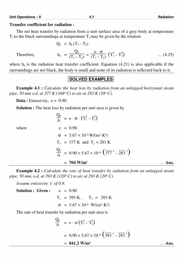
Unit Operations – II 4.7 Radiation
Transfer coefficient for radiation :
The net heat transfer by radiation from a unit surface area of a grey body at temperature
T1 to the black surroundings at temperature T2 may be given by the relation
Qr = hr (T1 – T2)
Therefore, hr = Qr
(T1 – T2) =
e · σ
(T1 – T2) ( )T
4
1 – T4
2 … (4.25)
where hr is the radiation heat transfer coefficient. Equation (4.21) is also applicable if the
surroundings are not black, the body is small and none of its radiation is reflected back to it.
SOLVED EXAMPLES
Example 4.1 : Calculate the heat loss by radiation from an unlagged horizontal steam
pipe, 50 mm o.d. at 377 K (104o C) to air at 283 K (10o C).
Data : Emissivity, e = 0.90.
Solution : The heat loss by radiation per unit area is given by
Qr
A = e · σ · ( )T
4
1 – T4
2
where e = 0.90
σ = 5.67 × 10⁻⁸ W/(m2·K4)
T1 = 377 K and T2 = 283 K
Qr
A = 0.90 × 5.67 × 10–8 ( )–––
377 4 –
–––283
4
= 704 W/m2 … Ans.
Example 4.2 : Calculate the rate of heat transfer by radiation from an unlagged steam
pipe, 50 mm, o.d. at 393 K (120o C) to air at 293 K (20o C).
Assume emissivity 'e' of 0.9.
Solution : Given : e = 0.90
T1 = 393 K , T2 = 293 K
σ = 5.67 × 10⁻⁸ W/(m2·K4)
The rate of heat transfer by radiation per unit area is
Qr
A = e · σ ( )T
4
1 – T4
2
= 0.90 × 5.67 × 10–8 ( )–––393
4 –
–––293
4
= 841.2 W/m2 … Ans.
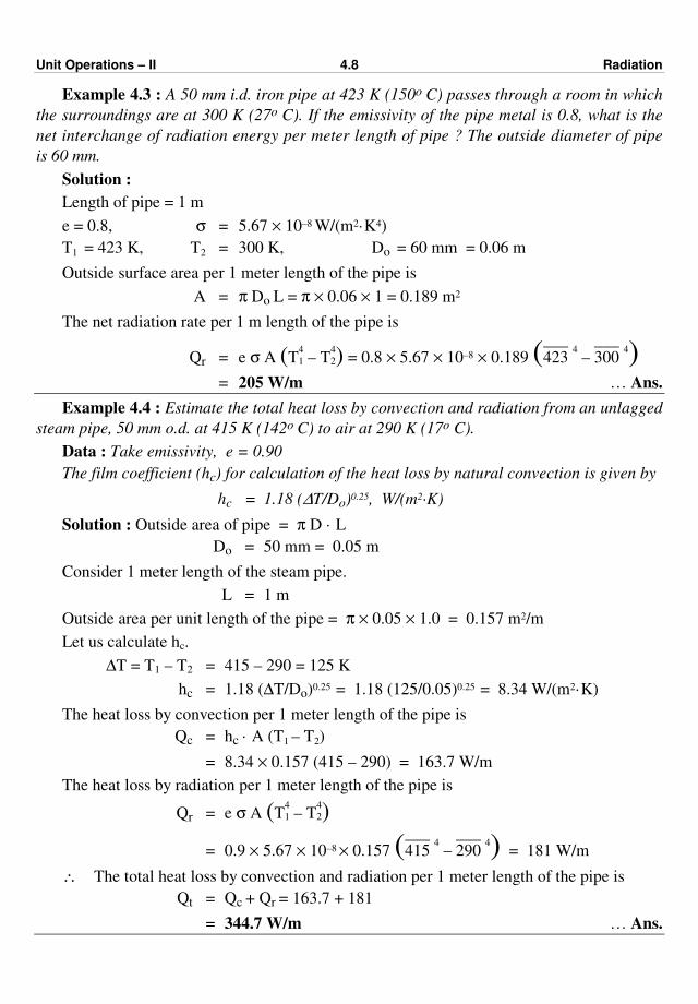
Unit Operations – II 4.8 Radiation
Example 4.3 : A 50 mm i.d. iron pipe at 423 K (150o C) passes through a room in which
the surroundings are at 300 K (27o C). If the emissivity of the pipe metal is 0.8, what is the
net interchange of radiation energy per meter length of pipe ? The outside diameter of pipe
is 60 mm.
Solution :
Length of pipe = 1 m
e = 0.8, σ = 5.67 × 10⁻⁸ W/(m2·K4)
T1 = 423 K, T2 = 300 K, Do = 60 mm = 0.06 m
Outside surface area per 1 meter length of the pipe is
A = π Do L = π × 0.06 × 1 = 0.189 m2
The net radiation rate per 1 m length of the pipe is
Qr = e σ A ( )T4
1 – T4
2 = 0.8 × 5.67 × 10–8 × 0.189 ( )–––423
4 –
–––300
4
= 205 W/m … Ans.
Example 4.4 : Estimate the total heat loss by convection and radiation from an unlagged
steam pipe, 50 mm o.d. at 415 K (142o C) to air at 290 K (17o C).
Data : Take emissivity, e = 0.90
The film coefficient (hc) for calculation of the heat loss by natural convection is given by
hc = 1.18 (∆T/Do)0.25, W/(m2·K)
Solution : Outside area of pipe = π D · L
Do = 50 mm = 0.05 m
Consider 1 meter length of the steam pipe.
L = 1 m
Outside area per unit length of the pipe = π × 0.05 × 1.0 = 0.157 m2/m
Let us calculate hc.
∆T = T1 – T2 = 415 – 290 = 125 K
hc = 1.18 (∆T/Do)0.25 = 1.18 (125/0.05)0.25 = 8.34 W/(m2·K)
The heat loss by convection per 1 meter length of the pipe is
Qc = hc · A (T1 – T2)
= 8.34 × 0.157 (415 – 290) = 163.7 W/m
The heat loss by radiation per 1 meter length of the pipe is
Qr = e σ A ( )T4
1 – T4
2
= 0.9 × 5.67 × 10–8 × 0.157 ( )–––415
4 –
–––290
4 = 181 W/m
∴ The total heat loss by convection and radiation per 1 meter length of the pipe is
Qt = Qc + Qr = 163.7 + 181
= 344.7 W/m … Ans.
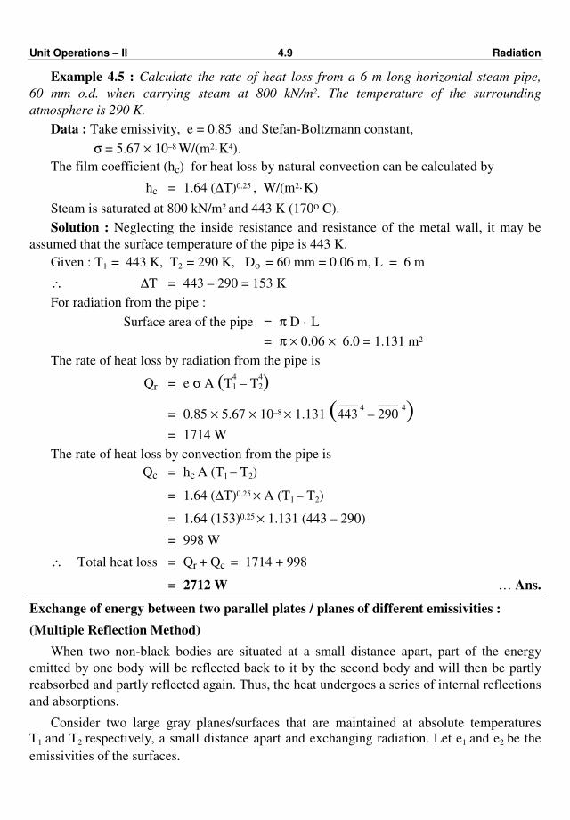
Unit Operations – II 4.9 Radiation
Example 4.5 : Calculate the rate of heat loss from a 6 m long horizontal steam pipe,
60 mm o.d. when carrying steam at 800 kN/m2. The temperature of the surrounding
atmosphere is 290 K.
Data : Take emissivity, e = 0.85 and Stefan-Boltzmann constant,
σ = 5.67 × 10⁻⁸ W/(m2·K4).
The film coefficient (hc) for heat loss by natural convection can be calculated by
hc = 1.64 (∆T)0.25 , W/(m2·K)
Steam is saturated at 800 kN/m2 and 443 K (170o C).
Solution : Neglecting the inside resistance and resistance of the metal wall, it may be
assumed that the surface temperature of the pipe is 443 K.
Given : T1 = 443 K, T2 = 290 K, Do = 60 mm = 0.06 m, L = 6 m
∴ ∆T = 443 – 290 = 153 K
For radiation from the pipe :
Surface area of the pipe = π D · L
= π × 0.06 × 6.0 = 1.131 m2
The rate of heat loss by radiation from the pipe is
Qr = e σ A ( )T4
1 – T4
2
= 0.85 × 5.67 × 10–8 × 1.131 ( )–––443
4 –
–––290
4
= 1714 W
The rate of heat loss by convection from the pipe is
Qc = hc A (T1 – T2)
= 1.64 (∆T)0.25 × A (T1 – T2)
= 1.64 (153)0.25 × 1.131 (443 – 290)
= 998 W
∴ Total heat loss = Qr + Qc = 1714 + 998
= 2712 W … Ans.
Exchange of energy between two parallel plates / planes of different emissivities :
(Multiple Reflection Method)
When two non-black bodies are situated at a small distance apart, part of the energy
emitted by one body will be reflected back to it by the second body and will then be partly
reabsorbed and partly reflected again. Thus, the heat undergoes a series of internal reflections
and absorptions.
Consider two large gray planes/surfaces that are maintained at absolute temperatures
T1 and T2 respectively, a small distance apart and exchanging radiation. Let e1 and e2 be the
emissivities of the surfaces.

Unit Operations – II 4.10 Radiation
Surface 2
Surface 1
se e21 se e (1 – e ) (1 – e )1 2 1 2
se (1 – e )1 2 se e (1 – e ) (1 – e )1 2 1 22
T2
T1
se1 se e (1 – e ) (1 – e )1 2 1 2se e (1 – e ) (1 – e )
2
1 2 1 2
2
Fig. 4.3 : Radiant heat exchanger between infinite parallel surfaces
(energy originating at surface-1 absorbed by surface-2)
Consider the energy radiated/emitted from the surface-1. Then, per unit area per unit time,
we have :
– energy radiated from surface 1 = σ · e1 T4
1 … (a)
– of this, energy absorbed by surface 2 = σ e1 T4
1 e2 … (b)
– and energy reflected by surface 2 = e1 T4
1 (1 – e2) … (c)
– of this, energy re-absorbed by surface 1 = σ e1 T4
1 (1 – e2) e1 … (d)
– and energy re-reflected by surface 1 = σ e1 T4
1 (1 – e2) (1 – e1) … (e)
– and of this, energy absorbed by surface 2 = σ e1 T4
1 (1 – e2) (1 – e1) e2 … (f)
Hence, as a result of each complete cycle of internal reflection, it is clear by comparing
(b) and (f) that the absorption is reduced by a factor (1 – e1) (1 – e2). As the energy suffers an
infinite number of reflections, we can write :
Total transfer of energy from surface 1 to surface 2 per unit area and unit time is
(Q/A)1–2 = σ · e1 e2 T4
1 [1 + (1 – e1) (1 – e2) + (1 – e1)2 (1 – e2)2 … to ∞]
= σ · e1 e2 T4
1 1
1 – (1 – e1) (1 – e2)
= σ · e1 e2
e1 + e2 – e1 e2 T
4
1
In a similar manner, considering the radiation emitted by the surface 2, it can be shown
that the total transfer of energy from surface 2 to surface 1 per unit area per unit time
(i.e., emitted by the surface 2 and absorbed by the surface 1) is
(Q/A)2–1 = e1 e2 σ
e1 + e2 – e1 e2 T
4
2
Thus, the net energy transferred per unit area per unit time is
Q
A12
= e1 e2 σ
e1 + e2 – e1 e2 ( )T
4
1 – T4
2
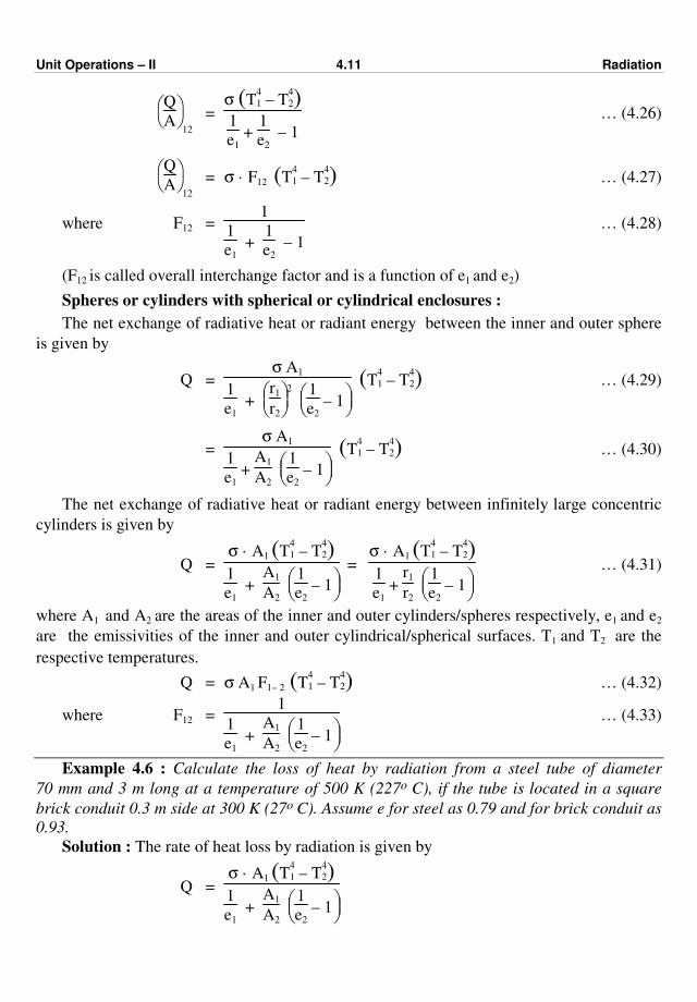
Unit Operations – II 4.11 Radiation
Q
A12
= σ ( )T
4
1 – T4
2
1
e1 +
1
e2 – 1
… (4.26)
Q
A12
= σ · F12 ( )T4
1 – T4
2 … (4.27)
where F12 = 1
1
e1 +
1
e2 – 1
… (4.28)
(F12 is called overall interchange factor and is a function of e1 and e2)
Spheres or cylinders with spherical or cylindrical enclosures :
The net exchange of radiative heat or radiant energy between the inner and outer sphere
is given by
Q = σ A1
1
e1 +
r1
r2
2
1
e2 – 1
( )T4
1 – T4
2 … (4.29)
= σ A1
1
e1 +
A1
A2
1
e2 – 1
( )T4
1 – T4
2 … (4.30)
The net exchange of radiative heat or radiant energy between infinitely large concentric
cylinders is given by
Q = σ · A1 ( )T
4
1 – T4
2
1
e1 +
A1
A2
1
e2 – 1
= σ · A1 ( )T
4
1 – T4
2
1
e1 +
r1
r2
1
e2 – 1
… (4.31)
where A1 and A2 are the areas of the inner and outer cylinders/spheres respectively, e1 and e2
are the emissivities of the inner and outer cylindrical/spherical surfaces. T1 and T2 are the
respective temperatures.
Q = σ A1 F1– 2 ( )T4
1 – T4
2 … (4.32)
where F12 = 1
1
e1 +
A1
A2
1
e2 – 1
… (4.33)
Example 4.6 : Calculate the loss of heat by radiation from a steel tube of diameter
70 mm and 3 m long at a temperature of 500 K (227o C), if the tube is located in a square
brick conduit 0.3 m side at 300 K (27o C). Assume e for steel as 0.79 and for brick conduit as
0.93.
Solution : The rate of heat loss by radiation is given by
Q = σ · A1 ( )T
4
1 – T4
2
1
e1 +
A1
A2
1
e2 – 1
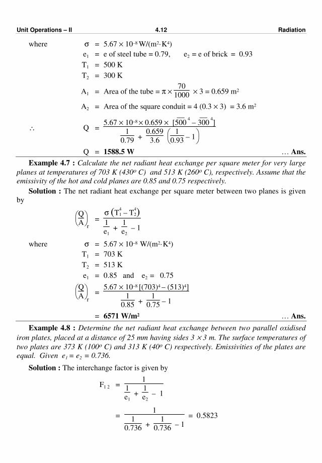
Unit Operations – II 4.12 Radiation
where σ = 5.67 × 10⁻⁸ W/(m2·K4)
e1 = e of steel tube = 0.79, e2 = e of brick = 0.93
T1 = 500 K
T2 = 300 K
A1 = Area of the tube = π × 70
1000 × 3 = 0.659 m2
A2 = Area of the square conduit = 4 (0.3 × 3) = 3.6 m2
∴ Q = 5.67 × 10–8 × 0.659 × [
––500
4 –
––300
4]
1
0.79 +
0.659
3.6
1
0.93 – 1
Q = 1588.5 W … Ans.
Example 4.7 : Calculate the net radiant heat exchange per square meter for very large
planes at temperatures of 703 K (430o C) and 513 K (260o C), respectively. Assume that the
emissivity of the hot and cold planes are 0.85 and 0.75 respectively.
Solution : The net radiant heat exchange per square meter between two planes is given
by
Q
Ar =
σ ( )T4
1 – T4
2
1
e1 +
1
e2 – 1
where σ = 5.67 × 10⁻⁸ W/(m2·K4)
T1 = 703 K
T2 = 513 K
e1 = 0.85 and e2 = 0.75
Q
Ar =
5.67 × 10⁻⁸ [(703)4 – (513)4]
1
0.85 +
1
0.75 – 1
= 6571 W/m2 … Ans.
Example 4.8 : Determine the net radiant heat exchange between two parallel oxidised
iron plates, placed at a distance of 25 mm having sides 3 × 3 m. The surface temperatures of
two plates are 373 K (100o C) and 313 K (40o C) respectively. Emissivities of the plates are
equal. Given e1 = e2 = 0.736.
Solution : The interchange factor is given by
F1 2 = 1
1
e1 +
1
e2 – 1
= 1
1
0.736 +
1
0.736 – 1
= 0.5823
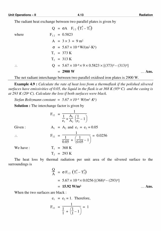
Unit Operations – II 4.13 Radiation
The radiant heat exchange between two parallel plates is given by
Q = σA F1 2 ( )T4
1 – T4
2
where F1 2 = 0.5823
A = 3 × 3 = 9 m2
σ = 5.67 × 10⁻⁸ W/(m2·K4)
T1 = 373 K
T2 = 313 K
∴ Q = 5.67 × 10–8 × 9 × 0.5823 × [(373)4 – (313)4]
= 2900 W … Ans.
The net radiant interchange between two parallel oxidised iron plates is 2900 W.
Example 4.9 : Calculate the rate of heat loss from a thermoflask if the polished silvered
surfaces have emissivities of 0.05, the liquid in the flask is at 368 K (95o C) and the casing is
at 293 K (20o C). Calculate the loss if both surfaces were black.
Stefan Boltzmann constant = 5.67 × 10⁻⁸ W/(m2 ·K4)
Solution : The interchange factor is given by
F12 = 1
1
e1 +
A1
A2
1
e2 – 1
Given : A1 = A2 and e1 = e2 = 0.05
∴ F12 = 1
1
0.05 +
1
0.05 – 1
= 0.0256
We have : T1 = 368 K
T2 = 293 K
The heat loss by thermal radiation per unit area of the silvered surface to the
surroundings is
Q
A = σ F1 2 ( )T
4
1 – T4
2
= 5.67 × 10–8 × 0.0256 [(368)4 – (293)4]
= 15.92 W/m2 … Ans.
When the two surfaces are black :
e1 = e2 = 1. Therefore,
F12 = 1
1
1 +
1
1 – 1
= 1
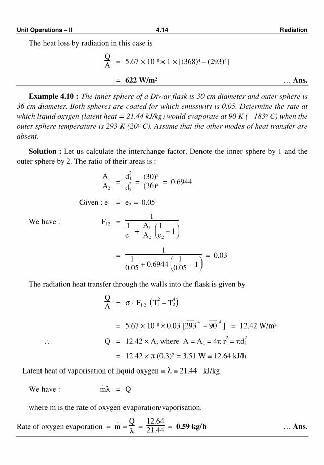
Unit Operations – II 4.14 Radiation
The heat loss by radiation in this case is
Q
A = 5.67 × 10–8 × 1 × [(368)4 – (293)4]
= 622 W/m2 … Ans.
Example 4.10 : The inner sphere of a Diwar flask is 30 cm diameter and outer sphere is
36 cm diameter. Both spheres are coated for which emissivity is 0.05. Determine the rate at
which liquid oxygen (latent heat = 21.44 kJ/kg) would evaporate at 90 K (– 183o C) when the
outer sphere temperature is 293 K (20o C). Assume that the other modes of heat transfer are
absent.
Solution : Let us calculate the interchange factor. Denote the inner sphere by 1 and the
outer sphere by 2. The ratio of their areas is :
A1
A2 =
d2
1
d2
2
= (30)2
(36)2 = 0.6944
Given : e1 = e2 = 0.05
We have : F12 = 1
1
e1 +
A1
A2
1
e2 – 1
= 1
1
0.05 + 0.6944
1
0.05 – 1
= 0.03
The radiation heat transfer through the walls into the flask is given by
Q
A = σ · F1 2 ( )T
2
1 – T4
2
= 5.67 × 10–8 × 0.03 [––
293 4
– ––90
4 ] = 12.42 W/m2
∴ Q = 12.42 × A, where A = A1 = 4π r2
1 = πd2
1
= 12.42 × π (0.3)2 = 3.51 W ≡ 12.64 kJ/h
Latent heat of vaporisation of liquid oxygen = λ = 21.44 kJ/kg
We have : ⋅
mλ = Q
where ⋅
m is the rate of oxygen evaporation/vaporisation.
Rate of oxygen evaporation = ⋅
m = Q
λ =
12.64
21.44 = 0.59 kg/h … Ans.
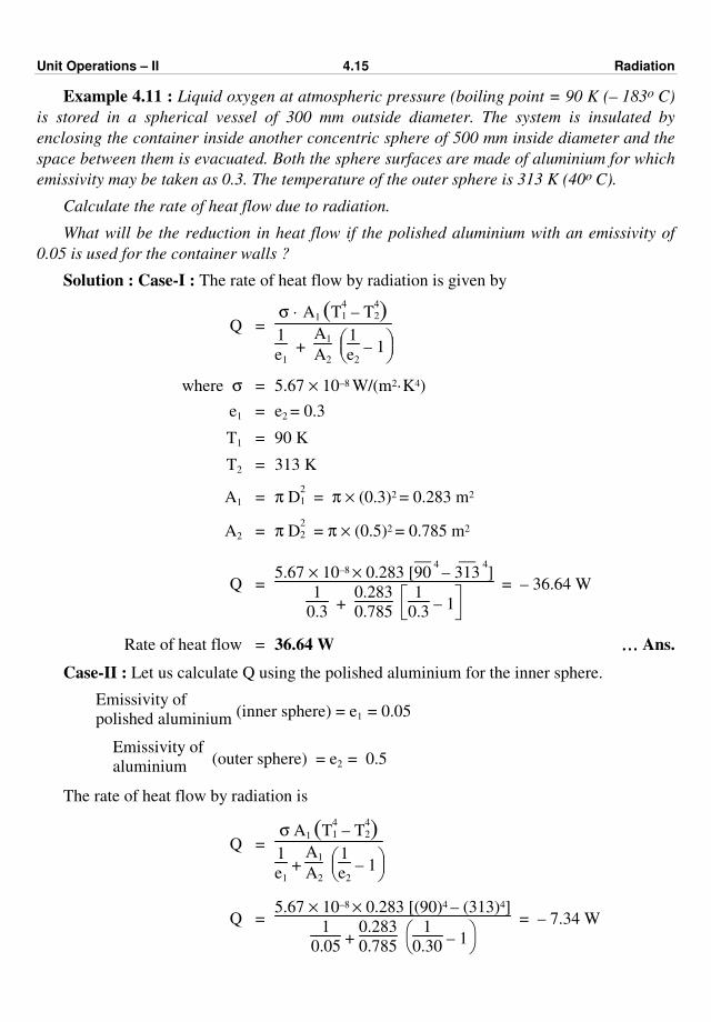
Unit Operations – II 4.15 Radiation
Example 4.11 : Liquid oxygen at atmospheric pressure (boiling point = 90 K (– 183o C)
is stored in a spherical vessel of 300 mm outside diameter. The system is insulated by
enclosing the container inside another concentric sphere of 500 mm inside diameter and the
space between them is evacuated. Both the sphere surfaces are made of aluminium for which
emissivity may be taken as 0.3. The temperature of the outer sphere is 313 K (40o C).
Calculate the rate of heat flow due to radiation.
What will be the reduction in heat flow if the polished aluminium with an emissivity of
0.05 is used for the container walls ?
Solution : Case-I : The rate of heat flow by radiation is given by
Q = σ · A1 ( )T
4
1 – T4
2
1
e1 +
A1
A2
1
e2 – 1
where σ = 5.67 × 10⁻⁸ W/(m2·K4)
e1 = e2 = 0.3
T1 = 90 K
T2 = 313 K
A1 = π D2
1 = π × (0.3)2 = 0.283 m2
A2 = π D2
2 = π × (0.5)2 = 0.785 m2
Q = 5.67 × 10–8 × 0.283 [
––90
4 –
––313
4]
1
0.3 +
0.283
0.785
1
0.3 – 1
= – 36.64 W
Rate of heat flow = 36.64 W ………… Ans.
Case-II : Let us calculate Q using the polished aluminium for the inner sphere.
Emissivity of
polished aluminium (inner sphere) = e1 = 0.05
Emissivity of
aluminium (outer sphere) = e2 = 0.5
The rate of heat flow by radiation is
Q = σ A1 ( )T
4
1 – T4
2
1
e1 +
A1
A2
1
e2 – 1
Q = 5.67 × 10–8 × 0.283 [(90)4 – (313)4]
1
0.05 +
0.283
0.785
1
0.30 – 1
= – 7.34 W
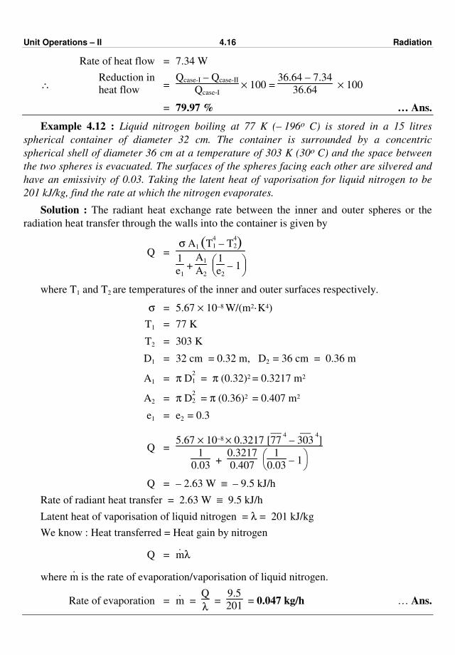
Unit Operations – II 4.16 Radiation
Rate of heat flow = 7.34 W
∴ Reduction in
heat flow = Qcase-I – Qcase-II
Qcase-I × 100 =
36.64 – 7.34
36.64 × 100
= 79.97 % … Ans.
Example 4.12 : Liquid nitrogen boiling at 77 K (– 196o C) is stored in a 15 litres
spherical container of diameter 32 cm. The container is surrounded by a concentric
spherical shell of diameter 36 cm at a temperature of 303 K (30o C) and the space between
the two spheres is evacuated. The surfaces of the spheres facing each other are silvered and
have an emissivity of 0.03. Taking the latent heat of vaporisation for liquid nitrogen to be
201 kJ/kg, find the rate at which the nitrogen evaporates.
Solution : The radiant heat exchange rate between the inner and outer spheres or the
radiation heat transfer through the walls into the container is given by
Q = σ A1 ( )T
4
1 – T4
2
1
e1 +
A1
A2
1
e2 – 1
where T1 and T2 are temperatures of the inner and outer surfaces respectively.
σ = 5.67 × 10⁻⁸ W/(m2·K4)
T1 = 77 K
T2 = 303 K
D1 = 32 cm = 0.32 m, D2 = 36 cm = 0.36 m
A1 = π D2
1 = π (0.32)2 = 0.3217 m2
A2 = π D2
2 = π (0.36)2 = 0.407 m2
e1 = e2 = 0.3
Q = 5.67 × 10–8 × 0.3217 [
––77
4 –
––303
4]
1
0.03 +
0.3217
0.407
1
0.03 – 1
Q = – 2.63 W ≡ – 9.5 kJ/h
Rate of radiant heat transfer = 2.63 W ≡ 9.5 kJ/h
Latent heat of vaporisation of liquid nitrogen = λ = 201 kJ/kg
We know : Heat transferred = Heat gain by nitrogen
Q = ⋅
mλ
where ⋅
m is the rate of evaporation/vaporisation of liquid nitrogen.
Rate of evaporation = ⋅
m = Q
λ =
9.5
201 = 0.047 kg/h … Ans.
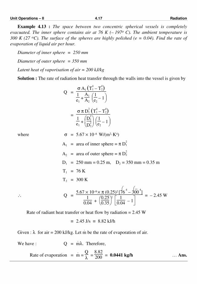
Unit Operations – II 4.17 Radiation
Example 4.13 : The space between two concentric spherical vessels is completely
evacuated. The inner sphere contains air at 76 K (– 197o C). The ambient temperature is
300 K (27 oC). The surface of the spheres are highly polished (e = 0.04). Find the rate of
evaporation of liquid air per hour.
Diameter of inner sphere = 250 mm
Diameter of outer sphere = 350 mm
Latent heat of vaporisation of air = 200 kJ/kg
Solution : The rate of radiation heat transfer through the walls into the vessel is given by
Q = σ A1 ( )T
4
1 – T4
2
1
e1 +
A1
A2
1
e2 – 1
= σ π D
2
1 ( )T4
1 – T4
2
1
e1 +
D
2
1
D2
2
1
e2 – 1
where σ = 5.67 × 10⁻⁸ W/(m2·K4)
A1 = area of inner sphere = π D2
1
A2 = area of outer sphere = π D2
2
D1 = 250 mm = 0.25 m, D2 = 350 mm = 0.35 m
T1 = 76 K
T2 = 300 K
∴ Q = 5.67 × 10⁻⁸ × π (0.25)2 [
76
4 –
–300
4]
1
0.04 +
0.25
0.35
2
1
0.04 – 1
= – 2.45 W
Rate of radiant heat transfer or heat flow by radiation = 2.45 W
≡ 2.45 J/s ≡ 8.82 kJ/h
Given : λ for air = 200 kJ/kg. Let ⋅
m be the rate of evaporation of air.
We have : Q = ⋅
mλ. Therefore,
Rate of evaporation = ⋅
m = Q
λ =
8.82
200 = 0.0441 kg/h … Ans.

Unit Operations – II 4.18 Radiation
EXERCISE
1. Fill in the blanks :
(a) Radiation refers to the transport of energy through space by ........... waves.
Ans. electromagnetic
(b) Heat can be transmitted by .......... mode across absolute vacuum. Ans. radiation
(c) The fraction of the incident radiation absorbed is known as ........ Ans. absorptivity
(d) For a perfectly black body absorptivity is equal to .......... Ans. one
(e) For a specular body the reflectivity is equal to ......... Ans. one
(f) As per Kirchhoff's law, at thermal equilibrium for all bodies the ratio of ..... to the
absorptivity will be the same. Ans. emissive power
(g) The emissivity 'e' of a body is equal to its ............. 'a'. Ans. absorptivity
(h) As per the Stefan-Boltzmann law the total energy emitted by a black body is directly
proportional to the fourth power of its absolute ......... Ans. temperature
(i) ............. Boltzmann equation is a fundamental relation for all radiant energy transfer
calculations. Ans. Stefan
(j) Emissivity of any body is the ratio of its ..... to that of a black body at the same
temperature. Ans. emissive power
2. Define the following terms :
(a) Radiation (b) Absorptivity (c) Emissivity (d) Opaque material (e) Gray body.
3. What do you mean by black body ?
4. Give examples of radiation heat transfer.
5. State Kirchhoff's law of radiation.
6. State Stefan-Boltzmann law of radiation.
7. Explain in brief the concept of black body.
8. Calculate the loss of heat per unit area from a steam pipe to the surrounding air by
radiation mode. Take emissivity of 0.90.
Data : Temperature of steam pipe = 398 K (125°C)
Temperature of air = 303 K (30°C) Ans. 851 W/m2
ppp
(5.1)
CHAPTER FIVE
HEAT EXCHANGE EQUIPMENTS
Various types of heat transfer equipments are used in the chemical industry depending
upon the applications involved (i.e., based on the service required), but their common task is
to transfer heat from a hot fluid to a cold fluid. The heat exchange equipments involve heat
energy transfer either by conduction-convection or by radiation mode. In the chemical
industry, shell and tube type heat exchangers constitute the bulk of unfired heat transfer
equipment.
A heat exchanger is a device used to effect the process of heat exchange between two
fluids that are at different temperatures. Recuperators (also called as surface heat
exchangers) are heat exchangers in which the fluids are separated by a metal wall, e.g., steam
boilers, heater, condensers, etc.
Based upon the function, heat transfer equipments can be referred as cooler, heater,
condenser, etc.
Cooler : It is a heat exchange equipment used to cool a process fluid (gas or liquid) by means of
water or atmospheric air. It involves the removal of sensible heat from the process fluid
(stream).
Condenser :
It is a heat exchange equipment used to condense a vapour or a mixture of vapours
(in the presence or absence of noncondensable gas). It involves the removal of latent heat
with the help of a suitable cooling medium, e.g., cooling tower water or chilled water.
Chiller :
It is a heat exchange equipment employed to cool a process fluid (stream) to a
temperature below that can be obtained by using water as a cooling medium. It employs a
refrigerant such as ammonia or freon as a cooling medium.
Exchanger :
It is a heat exchange equipment that is used to exchange the heat between hot and cold
process streams/fluids.
Heater :
It is a heat exchange equipment which imparts sensible heat to a process fluid (stream).
Condensing steam or dowtherm may be used as a heating medium.
It heats a process stream by condensing steam.
Reboiler :
It is a heat exchange equipment, used to meet the latent heat requirement at the bottom of
a distillation column. The heating medium may be either steam or a hot process fluid.
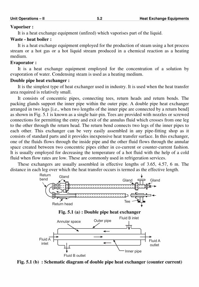
Unit Operations – II 5.2 Heat Exchange Equipments
Vaporiser :
It is a heat exchange equipment (unfired) which vaporises part of the liquid.
Waste - heat boiler :
It is a heat exchange equipment employed for the production of steam using a hot process
stream or a hot gas or a hot liquid stream produced in a chemical reaction as a heating
medium.
Evaporator :
It is a heat exchange equipment employed for the concentration of a solution by
evaporation of water. Condensing steam is used as a heating medium.
Double pipe heat exchanger :
It is the simplest type of heat exchanger used in industry. It is used when the heat transfer
area required is relatively small.
It consists of concentric pipes, connecting tees, return heads and return bends. The
packing glands support the inner pipe within the outer pipe. A double pipe heat exchanger
arranged in two legs [i.e., when two lengths of the inner pipe are connected by a return bend]
as shown in Fig. 5.1 is known as a single hair-pin. Tees are provided with nozzles or screwed
connections for permitting the entry and exit of the annulus fluid which crosses from one leg
to the other through the return head. The return bend connects two legs of the inner pipes to
each other. This exchanger can be very easily assembled in any pipe-fitting shop as it
consists of standard parts and it provides inexpensive heat transfer surface. In this exchanger,
one of the fluids flows through the inside pipe and the other fluid flows through the annular
space created between two concentric pipes either in co-current or counter-current fashion.
It is usually employed for decreasing the temperature of a hot fluid with the help of a cold
fluid when flow rates are low. These are commonly used in refrigeration services.
These exchangers are usually assembled in effective lengths of 3.65, 4.57, 6 m. The
distance in each leg over which the heat transfer occurs is termed as the effective length.
Tee
Gland Gland
Returnbend
Gland
Return head
Fig. 5.1 (a) : Double pipe heat exchanger
Annular space Outer pipe
Fluid B outletInner pipe
Fluid Ainlet
Fluid Aoutlet
Fluid B inlet
Fig. 5.1 (b) : Schematic diagram of double pipe heat exchanger (counter current)

Unit Operations – II 5.3 Heat Exchange Equipments
The major disadvantages of a double pipe heat exchanger are :
1. Small heat transfer surface in a large floor space as compared to other types (e.g.,
shell and tube heat exchanger).
2. Dismantling requires large time and
3. Maximum leakage points.
Apart from this, double pipe heat exchanger is very attractive where the total heat
transfer surface required is small, 9.29 m2 to 14 m2 or less. It is simple in construction, cheap
and easy to clean.
Shell and Tube Heat Exchanger :
For a variety of industrial services where large heat transfer surfaces are required, shell
and tube heat exchangers are commonly used. These heat exchange equipments can be
fabricated from a wide range of materials of construction.
A shell and tube heat exchanger consists of a number of parallel tubes, ends of which are
fixed in the tube sheets and the entire tube bundle is enclosed in a close fitting cylindrical
shell. In this exchanger, heat transfer surface is the one that is offered by tubes. One of the
fluid flows through the tubes, while the outer fluid flows through the space created between
tubes and shell, i.e., outside the tubes. These fluids are in thermal contact but are physically
separated by a metal wall of the tubes. Heat flows through the metal wall of the tubes from
the hot fluid to the cold fluid. The fluid flowing through the tubes is called the tube fluid/tube
side fluid, whereas the fluid flowing outside the tube is called the shell fluid/shell side fluid.
If none of the fluids condenses or evaporates, the unit is known as heat exchanger.
When one of the fluids condenses, then the unit is known as condenser or as heater
depending on whether the primary purpose of the unit is to condense one fluid or to heat the
other. Similarly such units may be called as cooler, evaporator, etc. based on a primary
purpose for which they are used.
Shell :
It is usually a cylindrical casing through which one of the fluids flows in one or more
passes. Shell is commonly made of carbon steel. It may be cut to the required length from a
standard pipe upto 60 cm diameter or fabricated from plates. The minimum thickness of shell
made of carbon steel varies from 5 mm to 11 mm depending upon the diameter.
Tubes :
Standard heat exchanger tubes used in many industrial processes may be of various sizes
and lengths. The outside diameter of tubes vary from 6 mm to 40 mm. The tubes with outside
diameters of 19 mm and 25 mm are very common. The tube lengths used are 0.5, 2.5, 3, 4, 5
and 6 meters. The wall thickness of tubes is usually expressed in terms of Birmingham Wire
Gauge (BWG). It depends upon the material of construction and diameter. For 19 or 25 mm
outside diameter tube of mild steel 10 or 12 BWG is common. The tubes that are placed in a
tube bundle inside the shell are either rolled or welded to the tube sheet. The tube side fluid
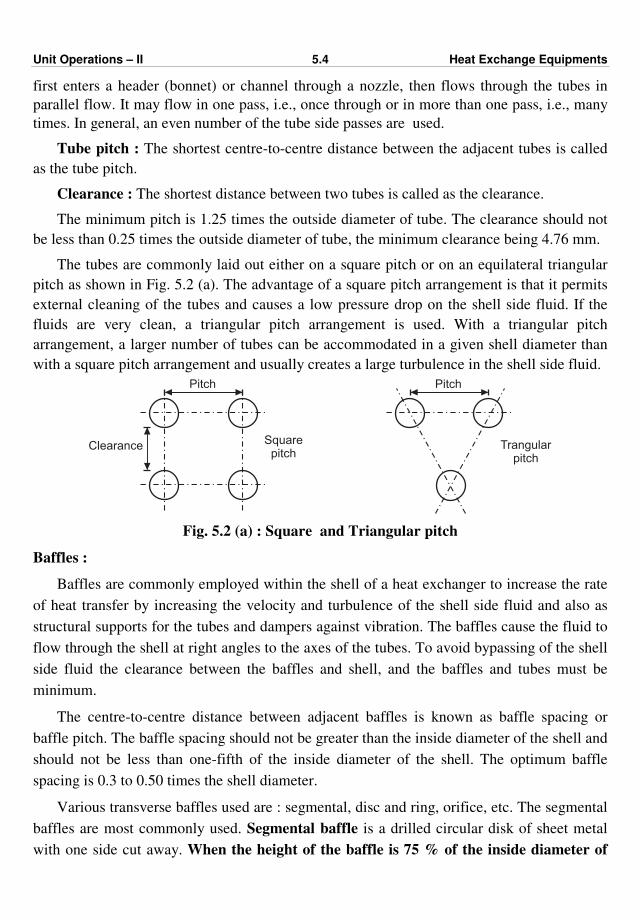
Unit Operations – II 5.4 Heat Exchange Equipments
first enters a header (bonnet) or channel through a nozzle, then flows through the tubes in
parallel flow. It may flow in one pass, i.e., once through or in more than one pass, i.e., many
times. In general, an even number of the tube side passes are used.
Tube pitch : The shortest centre-to-centre distance between the adjacent tubes is called
as the tube pitch.
Clearance : The shortest distance between two tubes is called as the clearance.
The minimum pitch is 1.25 times the outside diameter of tube. The clearance should not
be less than 0.25 times the outside diameter of tube, the minimum clearance being 4.76 mm.
The tubes are commonly laid out either on a square pitch or on an equilateral triangular
pitch as shown in Fig. 5.2 (a). The advantage of a square pitch arrangement is that it permits
external cleaning of the tubes and causes a low pressure drop on the shell side fluid. If the
fluids are very clean, a triangular pitch arrangement is used. With a triangular pitch
arrangement, a larger number of tubes can be accommodated in a given shell diameter than
with a square pitch arrangement and usually creates a large turbulence in the shell side fluid.
Squarepitch
Clearance
Pitch Pitch
Trangularpitch
Fig. 5.2 (a) : Square and Triangular pitch
Baffles :
Baffles are commonly employed within the shell of a heat exchanger to increase the rate
of heat transfer by increasing the velocity and turbulence of the shell side fluid and also as
structural supports for the tubes and dampers against vibration. The baffles cause the fluid to
flow through the shell at right angles to the axes of the tubes. To avoid bypassing of the shell
side fluid the clearance between the baffles and shell, and the baffles and tubes must be
minimum.
The centre-to-centre distance between adjacent baffles is known as baffle spacing or
baffle pitch. The baffle spacing should not be greater than the inside diameter of the shell and
should not be less than one-fifth of the inside diameter of the shell. The optimum baffle
spacing is 0.3 to 0.50 times the shell diameter.
Various transverse baffles used are : segmental, disc and ring, orifice, etc. The segmental
baffles are most commonly used. Segmental baffle is a drilled circular disk of sheet metal
with one side cut away. When the height of the baffle is 75 % of the inside diameter of
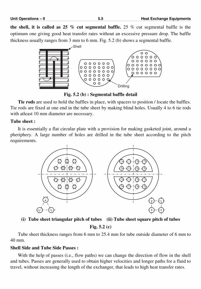
Unit Operations – II 5.5 Heat Exchange Equipments
the shell, it is called as 25 % cut segmental baffle. 25 % cut segmental baffle is the
optimum one giving good heat transfer rates without an excessive pressure drop. The baffle
thickness usually ranges from 3 mm to 6 mm. Fig. 5.2 (b) shows a segmental baffle.
Shell
Drilling
Fig. 5.2 (b) : Segmental baffle detail
Tie rods are used to hold the baffles in place, with spacers to position / locate the baffles.
Tie rods are fixed at one end in the tube sheet by making blind holes. Usually 4 to 6 tie rods
with atleast 10 mm diameter are necessary.
Tube sheet :
It is essentially a flat circular plate with a provision for making gasketed joint, around a
pheriphery. A large number of holes are drilled in the tube sheet according to the pitch
requirements.
(i) Tube sheet triangular pitch of tubes (ii) Tube sheet square pitch of tubes
Fig. 5.2 (c)
Tube sheet thickness ranges from 6 mm to 25.4 mm for tube outside diameter of 6 mm to
40 mm.
Shell Side and Tube Side Passes :
With the help of passes (i.e., flow paths) we can change the direction of flow in the shell
and tubes. Passes are generally used to obtain higher velocities and longer paths for a fluid to
travel, without increasing the length of the exchanger, that leads to high heat transfer rates.
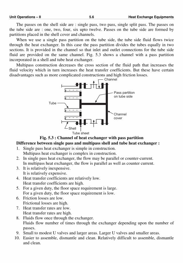
Unit Operations – II 5.6 Heat Exchange Equipments
The passes on the shell side are : single pass, two pass, single split pass. The passes on
the tube side are : one, two, four, six upto twelve. Passes on the tube side are formed by
partitions placed in the shell cover and channels.
When we use a single pass partition on the tube side, the tube side fluid flows twice
through the heat exchanger. In this case the pass partition divides the tubes equally in two
sections. It is provided in the channel so that inlet and outlet connections for the tube side
fluid are provided on the same channel. Fig. 5.3 shows a channel with a pass partition
incorporated in a shell and tube heat exchanger.
Multipass construction decreases the cross section of the fluid path that increases the
fluid velocity which in turn increases the heat transfer coefficients. But these have certain
disadvantages such as more complicated constructions and high friction losses. Channel
Pass partitionon tube side
Tube
Shell
Channelcover
Tube sheet Fig. 5.3 : Channel of heat exchanger with pass partition
Difference between single pass and multipass shell and tube heat exchanger :
1. Single pass heat exchanger is simple in construction.
Multipass heat exchanger is complex in construction.
2. In single pass heat exchanger, the flow may be parallel or counter-current.
In multipass heat exchanger, the flow is parallel as well as counter current.
3. It is relatively inexpensive.
It is relatively expensive.
4. Heat transfer coefficients are relatively low.
Heat transfer coefficients are high.
5. For a given duty, the floor space requirement is large.
For a given duty, the floor space requirement is low.
6. Friction losses are low.
Frictional losses are high.
7. Heat transfer rates are low.
Heat transfer rates are high.
8. Fluids flow once through the exchanger.
Fluids flow number of times through the exchanger depending upon the number of
passes.
9. Small to modest U valves and larger areas. Larger U valves and smaller areas.
10. Easier to assemble, dismantle and clean. Relatively difficult to assemble, dismantle
and clean.
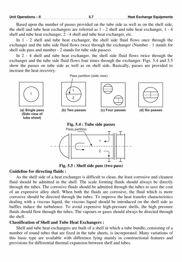
Unit Operations – II 5.7 Heat Exchange Equipments
Based upon the number of passes provided on the tube side as well as on the shell side,
the shell and tube heat exchangers are referred as 1 - 2 shell and tube heat exchanger, 1 - 4
shell and tube heat exchanger, 2 - 4 shell and tube heat exchanger, etc.
In 1 - 2 shell and tube heat exchanger, the shell side fluid flows once through the
exchanger and the tube side fluid flows twice through the exchanger (Number - 1 stands for
shell side pass and number - 2 stands for tube side passes).
In 2 - 4 shell and tube heat exchanger, the shell side fluid flows twice through the
exchanger and the tube side fluid flows four times through the exchanger. Figs. 5.4 and 5.5
show the passes on tube side as well as on shell side. Basically, passes are provided to
increase the heat recovery.
(a) Single pass(Side view oftube sheet)
(b) Two passes (c) Four passes (d) Six passes
11
2
Pass partition (side view)
Fig. 5.4 : Tube side passes Pass partition
1
2
Fig. 5.5 : Shell side pass (two pass)
Guideline for directing fluids :
As the shell side of a heat exchanger is difficult to clean, the least corrosive and cleanest
fluid should be admitted in the shell. The scale forming fluids should always be directly
through the tubes. The corrosive fluids should be admitted through the tubes to save the cost
of an expensive alloy shell. When both the fluids are corrosive, the fluid which is more
corrosive should be directed through the tubes. To improve the heat transfer characteristics
dealing with a viscous liquid, the viscous liquid should be introduced on the shell side as
baffles induce the turbulence. To avoid expensive high-pressure shells, the high pressure
fluids should flow through the tubes. The vapours or gases should always be directed through
the shell.
Classification of Shell and Tube Heat Exchangers :
Shell and tube heat exchangers are built of a shell in which a tube bundle, consisting of a
number of round tubes that are fixed in the tube sheets, is incorporated. Many variations of
this basic type are available with difference lying mainly in constructional features and
provisions for differential thermal expansion between shell and tubes.

Unit Operations – II 5.8 Heat Exchange Equipments
These exchangers are classified as :
1. Fixed tube sheet heat exchanger.
2. Floating head heat exchanger.
(a) Internal floating head and (b) Outside packed floating head
3. U-tube type heat exchanger and
4. Reboiler / Kettel type heat exchanger
(i) with internal floating head or (ii) with U-tube (hair pin).
The main components of all these exchangers are shell, shell cover, tubes, tube sheets,
channel, channel cover, nozzles (inlet/outlet), pass partitions, baffles, tie rods and
spacers.
Fixed tube-sheet exchanger :
This is the simplest form of heat exchanger wherein the tube sheets are welded to a shell
at both the ends. The shell is equipped with two nozzles. The tube sheets usually extend
beyond the shell and serve as flanges for the attachments of the channels on either side as
shown in Fig. 5.6. In a fixed tube type construction, the shell and tube sheet materials must
be weldable to each other. The channels on either sides are covered by means of channel
covers and are provided with nozzle connections for the entry and exist of the tube side fluid.
The shell side passes more than two are rarely used but as such there is no limitation on the
tube side passes.
In the another variation of fixed tube sheet heat exchanger shown in Fig. 5.7, a tube side
header (i.e., a channel) may be welded to the tube sheet and channels on the either sides are
closed with removable covers. In order to account for the differential expansion between
shell and tubes occurring because of differences in the thermal properties of materials of the
shell and tubes, expansion joints such as expansion bellows are used on the shell
(to eliminate excessive stresses caused by the thermal expansion).
ChannelShell fluid
inlet Tie rodBaffle
Fixedtubesheet
Tube Shell
Tube fluidinlet
Shell fluidoutlet
Channel
Channelcover
Tube fluidoutlet
Fig. 5.6 : Fixed tube sheet heat exchanger
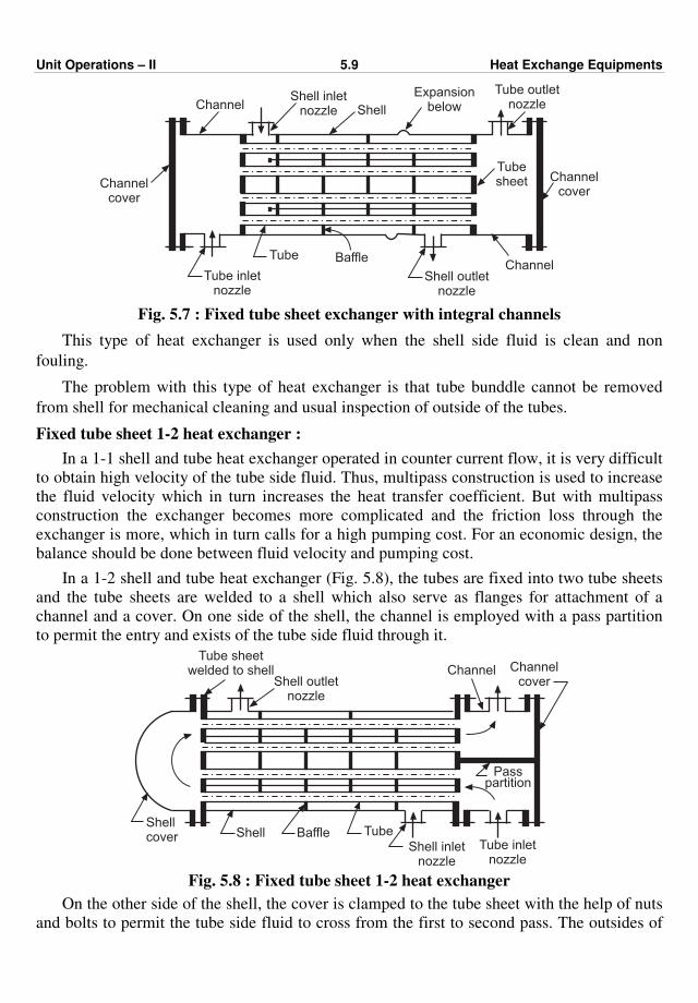
Unit Operations – II 5.9 Heat Exchange Equipments
ChannelShell inlet
nozzle
Tubesheet
Tube Baffle
Tube inletnozzle
Channel
Channelcover
Tube outletnozzleShell
Channelcover
Expansionbelow
Shell outletnozzle
Fig. 5.7 : Fixed tube sheet exchanger with integral channels
This type of heat exchanger is used only when the shell side fluid is clean and non
fouling.
The problem with this type of heat exchanger is that tube bunddle cannot be removed
from shell for mechanical cleaning and usual inspection of outside of the tubes.
Fixed tube sheet 1-2 heat exchanger :
In a 1-1 shell and tube heat exchanger operated in counter current flow, it is very difficult
to obtain high velocity of the tube side fluid. Thus, multipass construction is used to increase
the fluid velocity which in turn increases the heat transfer coefficient. But with multipass
construction the exchanger becomes more complicated and the friction loss through the
exchanger is more, which in turn calls for a high pumping cost. For an economic design, the
balance should be done between fluid velocity and pumping cost.
In a 1-2 shell and tube heat exchanger (Fig. 5.8), the tubes are fixed into two tube sheets
and the tube sheets are welded to a shell which also serve as flanges for attachment of a
channel and a cover. On one side of the shell, the channel is employed with a pass partition
to permit the entry and exists of the tube side fluid through it.
ChannelShell outlet
nozzle
Passpartition
TubeShellShell inlet
nozzle
Tube sheetwelded to shell
Baffle
Channelcover
Shellcover
Tube inletnozzle
Fig. 5.8 : Fixed tube sheet 1-2 heat exchanger
On the other side of the shell, the cover is clamped to the tube sheet with the help of nuts
and bolts to permit the tube side fluid to cross from the first to second pass. The outsides of
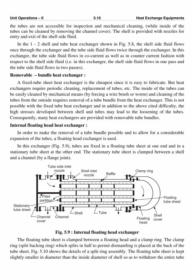
Unit Operations – II 5.10 Heat Exchange Equipments
the tubes are not accessible for inspection and mechanical cleaning, (while inside of the
tubes can be cleaned by removing the channel cover). The shell is provided with nozzles for
entry and exit of the shell side fluid.
In the 1 - 2 shell and tube heat exchanger shown in Fig. 5.8, the shell side fluid flows
once through the exchanger and the tube side fluid flows twice through the exchanger. In this
exchanger, the tube side fluid flows in co-current as well as in counter current fashion with
respect to the shell side fluid (i.e. in this exchanger, the shell side fluid flows in one pass and
the tube side fluid flows in two passes).
Removable – bundle heat exchanger :
A fixed-tube sheet heat exchanger is the cheapest since it is easy to fabricate. But heat
exchangers require periodic cleaning, replacement of tubes, etc. The inside of the tubes can
be easily cleaned by mechanical means (by forcing a wire brush or worm) and cleaning of the
tubes from the outside requires removal of a tube bundle from the heat exchanger. This is not
possible with the fixed tube heat exchanger and in addition to the above cited difficulty, the
high stresses developed between shell and tubes may lead to the loosening of the tubes.
Consequently, many heat exchangers are provided with removable tube bundles.
Internal floating head heat exchanger :
In order to make the removal of a tube bundle possible and to allow for a considerable
expansion of the tubes, a floating head exchanger is used.
In this exchanger (Fig. 5.9), tubes are fixed in a floating tube sheet at one end and in a
stationary tube sheet at the other end. The stationary tube sheet is clamped between a shell
and a channel (by a flange joint).
Clamp ringShell inletnozzle
TubeShell
Tube side inletnozzle
Floatingtube sheet
Floatinghead
Shellcover
Baffle
Passpartition
Channelcover
Channel
Stationarytube sheet
Fig. 5.9 : Internal floating head exchanger
The floating tube sheet is clamped between a floating head and a clamp ring. The clamp
ring (split backing ring) which splits in half to permit dismantling is placed at the back of the
tube sheet. Fig. 5.10 shows the details of a split ring assembly. The floating tube sheet is kept
slightly smaller in diameter than the inside diameter of shell so as to withdraw the entire tube

Unit Operations – II 5.11 Heat Exchange Equipments
bundle from the channel end. The channel is provided with inlet and outlet connections for
the tube side fluid. The shell is closed by a shell cover or bonnet on a floating head side.
Shell cover at the floating head end is larger than the other end so as to enable the tubes to be
placed as near as possible to the edge of the fixed tube sheet. The tube sheet along with the
floating head is free to move and thus, this exchanger takes into account differential thermal
expansion between shell and tubes.
Floatinghead cover
Splitring
Tubesheet
Fig. 5.10 : Split-ring assembly
It is widely used in chemical industries and petroleum refineries. It is suitable for severe
duties associated with high pressures and temperatures and also with dirty fluids.
Advantages :
(i) The tube bundle of the exchanger is removable for inspection and mechanical
cleaning of the tubes (from outside).
(ii) It eliminates differential expansion problems.
U-tube heat exchanger :
A U-tube 1-2 heat exchanger (shown in Fig. 5.11) consists of U-shaped tubes, both the
ends of which are fixed to a single stationary tube sheet. At one end of a shell, a channel is
provided with pass partition and is used for entry and exit of the tube side fluid. At the
opposite end of the shell, there is a cover which is integral with it. The shell is provided with
two nozzles for entry and exit of the shell side fluid. The tube sheet is clamped between shell
and channel flanges. The entire tube bundle can be removed from the shell from the channel
end. The differential thermal expansion between shell and tubes is absorbed by U-bends.
Each tube can expand or contract freely without affecting the other tubes. As there is a
limitation of bending tubes of a very short radius, the number of tube holes in the tube sheet
of a given diameter with this exchanger are less than those with a fixed tube sheet exchanger.
In this exchanger, the tube side fluid enters through the channel, it flows first through one
arm of the U - shaped tubes, it comes at the other end, travels down through the bend, flows
through the other arm of the U-shaped tubes and ultimately leaves the exchanger through an
outlet provided on the channel. During its passage through the exchanger, it exchanges heat
with the shell side fluid.
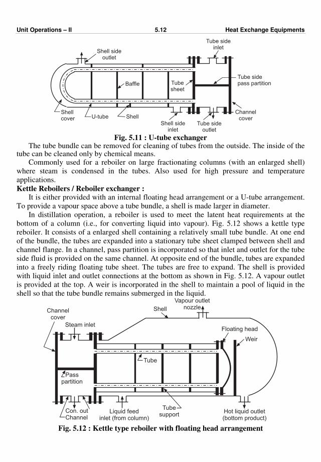
Unit Operations – II 5.12 Heat Exchange Equipments
Shell sideoutlet
U-tube
Shell sideinlet
Shell
Tube sideinlet
Shellcover
Tube sideoutlet
Tube sidepass partitionTube
sheetBaffle
Channelcover
Fig. 5.11 : U-tube exchanger
The tube bundle can be removed for cleaning of tubes from the outside. The inside of the tube can be cleaned only by chemical means. Commonly used for a reboiler on large fractionating columns (with an enlarged shell)
where steam is condensed in the tubes. Also used for high pressure and temperature
applications.
Kettle Reboilers / Reboiler exchanger : It is either provided with an internal floating head arrangement or a U-tube arrangement.
To provide a vapour space above a tube bundle, a shell is made larger in diameter.
In distillation operation, a reboiler is used to meet the latent heat requirements at the
bottom of a column (i.e., for converting liquid into vapour). Fig. 5.12 shows a kettle type
reboiler. It consists of a enlarged shell containing a relatively small tube bundle. At one end
of the bundle, the tubes are expanded into a stationary tube sheet clamped between shell and
channel flange. In a channel, pass partition is incorporated so that inlet and outlet for the tube
side fluid is provided on the same channel. At opposite end of the bundle, tubes are expanded
into a freely riding floating tube sheet. The tubes are free to expand. The shell is provided
with liquid inlet and outlet connections at the bottom as shown in Fig. 5.12. A vapour outlet
is provided at the top. A weir is incorporated in the shell to maintain a pool of liquid in the
shell so that the tube bundle remains submerged in the liquid.
Floating head
Tubesupport
Steam inlet
Hot liquid outlet(bottom product)
Shell
Passpartition
Con. outChannel
Liquid feedinlet (from column)
Weir
Vapour outletnozzle
Channelcover
Tube
Fig. 5.12 : Kettle type reboiler with floating head arrangement
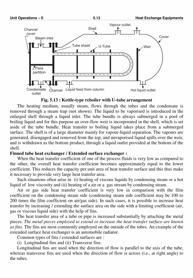
Unit Operations – II 5.13 Heat Exchange Equipments
CoverSteam inlet
Hot liquid outlet
Shell
Passpartition
Condensateoutlet
Channel
Weir
Vapour outlet
Channelcover
U-TubeTube sheet
Liquid feed from column
Fig. 5.13 : Kettle-type reboiler with U-tube arrangement
The heating medium, usually steam, flows through the tubes and the condensate is
removed through a steam trap (not shown). The liquid to be vaporised is introduced in the
enlarged shell through a liquid inlet. The tube bundle is always submerged in a pool of
boiling liquid and for this purpose an over-flow weir is incorporated in the shell, which is set
aside of the tube bundle. Heat transfer to boiling liquid takes place from a submerged
surface. The shell is of a large diameter mainly for vapour-liquid separation. The vapours are
generated, disengaged and removed from the top, and unvaporised liquid spills over the weir,
and is withdrawn as the bottom product, through a liquid outlet provided at the bottom of the
shell.
Finned tube heat exchanger / Extended surface exchanger : When the heat transfer coefficient of one of the process fluids is very low as compared to
the other, the overall heat transfer coefficient becomes approximately equal to the lower
coefficient. This reduces the capacity per unit area of heat transfer surface and this thus make
it necessary to provide very large heat transfer area.
Such situations often arise in (i) heating of viscous liquids by condensing steam or a hot
liquid of low viscosity and (ii) heating of a air or a gas stream by condensing steam.
Air or gas side heat transfer coefficient is very low in comparison with the film
coefficient on the condensing steam side (condensing steam side coefficient may be 100 to
200 times the film coefficient on air/gas side). In such cases, it is possible to increase heat
transfer by increasing / extending the surface area on the side with a limiting coefficient (air,
gas or viscous liquid side) with the help of fins.
The heat transfer area of a tube or pipe is increased substantially by attaching the metal
pieces. The metal pieces employed to extend or increase the heat transfer surface are known
as fins. The fins are most commonly employed on the outside of the tubes. An example of the
extended surface heat exchanger is an automobile radiator.
Common types of fins / extended surfaces are :
(i) Longitudinal fins and (ii) Transverse fins.
Longitudinal fins are used when the direction of flow is parallel to the axis of the tube,
whereas transverse fins are used when the direction of flow is across (i.e., at right angle) to
the tubes.
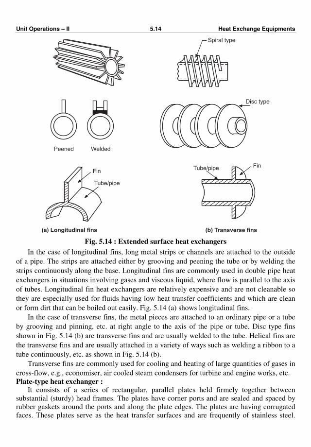
Unit Operations – II 5.14 Heat Exchange Equipments
Spiral type
Peened Welded
Fin
Tube/pipe
Tube/pipe Fin
Disc type
(a) Longitudinal fins (b) Transverse fins
Fig. 5.14 : Extended surface heat exchangers
In the case of longitudinal fins, long metal strips or channels are attached to the outside
of a pipe. The strips are attached either by grooving and peening the tube or by welding the
strips continuously along the base. Longitudinal fins are commonly used in double pipe heat
exchangers in situations involving gases and viscous liquid, where flow is parallel to the axis
of tubes. Longitudinal fin heat exchangers are relatively expensive and are not cleanable so
they are especially used for fluids having low heat transfer coefficients and which are clean
or form dirt that can be boiled out easily. Fig. 5.14 (a) shows longitudinal fins.
In the case of transverse fins, the metal pieces are attached to an ordinary pipe or a tube
by grooving and pinning, etc. at right angle to the axis of the pipe or tube. Disc type fins
shown in Fig. 5.14 (b) are transverse fins and are usually welded to the tube. Helical fins are
the transverse fins and are usually attached in a variety of ways such as welding a ribbon to a
tube continuously, etc. as shown in Fig. 5.14 (b).
Transverse fins are commonly used for cooling and heating of large quantities of gases in
cross-flow, e.g., economiser, air cooled steam condensers for turbine and engine works, etc.
Plate-type heat exchanger : It consists of a series of rectangular, parallel plates held firmely together between
substantial (sturdy) head frames. The plates have corner ports and are sealed and spaced by
rubber gaskets around the ports and along the plate edges. The plates are having corrugated
faces. These plates serve as the heat transfer surfaces and are frequently of stainless steel.

Unit Operations – II 5.15 Heat Exchange Equipments
Corrugated plates provide a high degree of turbulence even at low flow rates. In general,
a gap between plates is 1.3 to 1.5 mm. It is provided with inlet and outlet nozzles for fluids
at the ends.
In this exchanger, a hot fluid passes between alternate pairs of plates, transferring heat to
a cold fluid in the adjacent spaces.
The plates can be readily separated for cleaning and the heat transfer area can be
increased by simply adding more plates.
Advantages of plate heat exchanger : It being very compact requires a very small floor
space, low pressure drop, absence of inter leakage of fluids, ease in dismantling for the
inspection and cleaning of plates, high heat transfer coefficients, and provide a large heat
transfer areas in a small volume.
Plate heat exchangers are competitive with shell-and-tube exchangers where the
corrosion resistant materials are required. Since with these units the large surface is available
for a given duty, the operation with a small temperature difference is possible. Thus, for heat
sensitive materials and where a close temperature control is required, these units are used.
These are commonly used in dairy and brewery industries, where close control of
temperature is a valuable feature.
Plate exchangers are relatively effective with viscous fluids with viscosities upto about
30 kg/(m·s) (300 Poise). These can be used upto temperature of 423 K (150oC) and pressure
of 900 kN/m2. The weakness of these units is the necessity of long gaskets.
Fig. 5.15 shows a typical plate type unit.
Plate
In
Out
Head frame
Out
In
(a) (b)
Fixed endframe
Coldfluid in
Hot fluidout
Hot fluidin
Cold fluidout
++
++
++
++
Blind flange
Movable endframe
(c) (d)
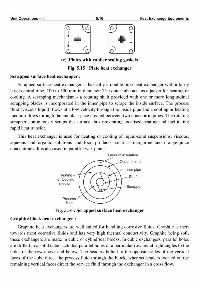
Unit Operations – II 5.16 Heat Exchange Equipments
(e) Plates with rubber sealing gaskets
Fig. 5.15 : Plate heat exchanger
Scrapped surface heat exchanger :
Scrapped surface heat exchanger is basically a double pipe heat exchanger with a fairly
large central tube, 100 to 300 mm in diameter. The outer tube acts as a jacket for heating or
cooling. A scrapping mechanism - a rotating shaft provided with one or more longitudinal
scrapping blades is incorporated in the inner pipe to scrape the inside surface. The process
fluid (viscous liquid) flows at a low velocity through the inside pipe and a cooling or heating
medium flows through the annular space created between two concentric pipes. The rotating
scrapper continuously scraps the surface thus preventing localised heating and facilitating
rapid heat transfer.
This heat exchanger is used for heating or cooling of liquid-solid suspensions, viscous,
aqueous and organic solutions and food products, such as margarine and orange juice
concentrates. It is also used in paraffin wax plants.
Heatingor Coolingmedium
Processfluid
Scrapper
Shaft
Inner pipe
Outside pipe
Layer of insulation
Fig. 5.16 : Scrapped surface heat exchanger
Graphite block heat exchanger :
Graphite heat exchangers are well suited for handling corrosive fluids. Graphite is inert
towards most corrosive fluids and has very high thermal conductivity. Graphite being soft,
these exchangers are made in cubic or cylindrical blocks. In cubic exchangers, parallel holes
are drilled in a solid cube such that parallel holes of a particular row are at right angles to the
holes of the row above and below. The headers bolted to the opposite sides of the vertical
faces of the cube direct the process fluid through the block, whereas headers located on the
remaining vertical faces direct the service fluid through the exchanger in a cross flow.
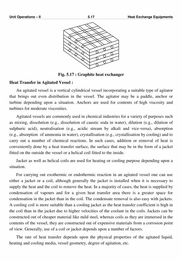
Unit Operations – II 5.17 Heat Exchange Equipments
Fig. 5.17 : Graphite heat exchanger
Heat Transfer in Agitated Vessel :
An agitated vessel is a vertical cylindrical vessel incorporating a suitable type of agitator
that brings out even distribution in the vessel. The agitator may be a paddle, anchor or
turbine depending upon a situation. Anchors are used for contents of high viscosity and
turbines for moderate viscosities.
Agitated vessels are commonly used in chemical industries for a variety of purposes such
as mixing, dissolution (e.g., dissolution of caustic soda in water), dilution (e.g., dilution of
sulphuric acid), neutralisation (e.g., acidic stream by alkali and vice-versa), absorption
(e.g., absorption of ammonia in water), crystallisation (e.g., crystallisation by cooling) and to
carry out a number of chemical reactions. In such cases, addition or removal of heat is
conveniently done by a heat transfer surface, the surface that may be in the form of a jacket
fitted on the outside the vessel or a helical coil fitted to the inside.
Jacket as well as helical coils are used for heating or cooling purpose depending upon a
situation.
For carrying out exothermic or endothermic reaction in an agitated vessel one can use
either a jacket or a coil, although generally the jacket is installed when it is necessary to
supply the heat and the coil to remove the heat. In a majority of cases, the heat is supplied by
condensation of vapours and for a given heat transfer area there is a greater space for
condensation in the jacket than in the coil. The condensate removal is also easy with jackets.
A cooling coil is more suitable than a cooling jacket as the heat transfer coefficient is high in
the coil than in the jacket due to higher velocities of the coolant in the coils. Jackets can be
constructed out of cheaper material like mild steel, whereas coils as they are immersed in the
contents of the vessel, they are constructed out of expensive materials from a corrosion point
of view. Generally, use of a coil or jacket depends upon a number of factors.
The rate of heat transfer depends upon the physical properties of the agitated liquid,
heating and cooling media, vessel geometry, degree of agitation, etc.

Unit Operations – II 5.18 Heat Exchange Equipments
Helicalcoil
Baffle
Agitator
Jacket
Vessel
Fig. 5.18 : Agitated vessel with jacket and helical coil
Film coefficients for jacket and coil :
(i) Coil :
hi-inside film coefficient is given by
hD
k = 0.023
Duρ
µ
0.8
Cp µ
k
a … (5.1)
where a = 0.4 for heating and 0.3 for cooling.
This equation is applicable for a straight tube.
For a coil, hi is given by
hi (coil) = hi (straight tube)
1 + 3.5 D
Dc … (5.2)
where D is the inside diameter of coil and Dc is the diameter of helix (coil diameter).
The agitator Reynolds number is given by
NRe, a = D
2
a Nρ
µ
For heating or cooling liquids in a baffled agitated vessel equipped with a helical coil and
a turbine agitator, hc is given by the following equation :
hc Dc
k = 0.17
D
2
a N ρ
µ
0.67
Cp µ
k
0.37
Da
Dt
Dc
Dt
0.5
µ
µw
0.24
… (5.3)
where Da = impeller diameter
Dt = vessel diameter
N = r.p.m.
and hc is the film coefficient between the coil surface and the liquid (the content of the
vessel).
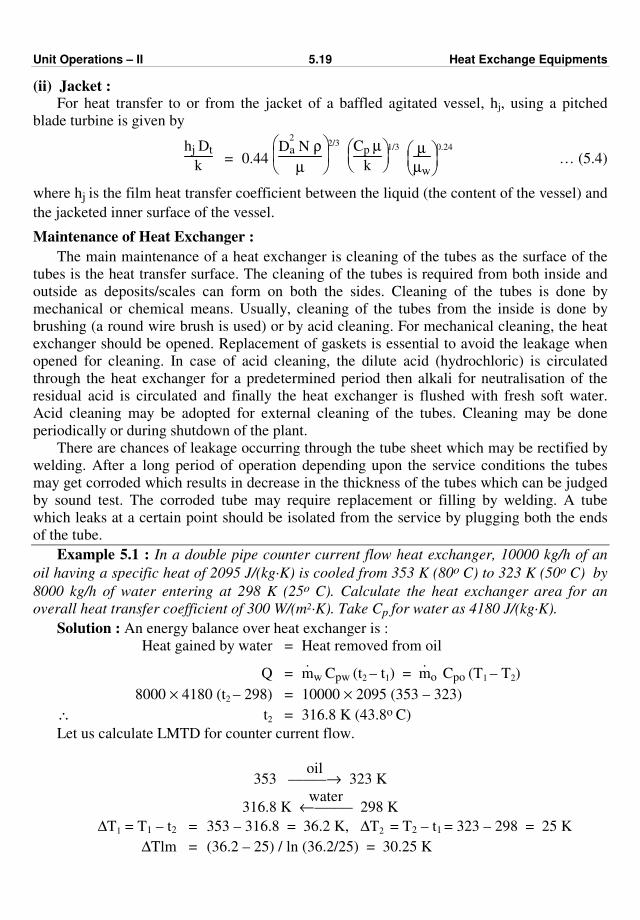
Unit Operations – II 5.19 Heat Exchange Equipments
(ii) Jacket : For heat transfer to or from the jacket of a baffled agitated vessel, hj, using a pitched
blade turbine is given by
hj Dt
k = 0.44
D
2
a N ρ
µ
2/3
Cp µ
k
1/3
µ
µw
0.24
… (5.4)
where hj is the film heat transfer coefficient between the liquid (the content of the vessel) and
the jacketed inner surface of the vessel.
Maintenance of Heat Exchanger :
The main maintenance of a heat exchanger is cleaning of the tubes as the surface of the
tubes is the heat transfer surface. The cleaning of the tubes is required from both inside and
outside as deposits/scales can form on both the sides. Cleaning of the tubes is done by
mechanical or chemical means. Usually, cleaning of the tubes from the inside is done by
brushing (a round wire brush is used) or by acid cleaning. For mechanical cleaning, the heat
exchanger should be opened. Replacement of gaskets is essential to avoid the leakage when
opened for cleaning. In case of acid cleaning, the dilute acid (hydrochloric) is circulated
through the heat exchanger for a predetermined period then alkali for neutralisation of the
residual acid is circulated and finally the heat exchanger is flushed with fresh soft water.
Acid cleaning may be adopted for external cleaning of the tubes. Cleaning may be done
periodically or during shutdown of the plant.
There are chances of leakage occurring through the tube sheet which may be rectified by
welding. After a long period of operation depending upon the service conditions the tubes
may get corroded which results in decrease in the thickness of the tubes which can be judged
by sound test. The corroded tube may require replacement or filling by welding. A tube
which leaks at a certain point should be isolated from the service by plugging both the ends
of the tube.
Example 5.1 : In a double pipe counter current flow heat exchanger, 10000 kg/h of an
oil having a specific heat of 2095 J/(kg·K) is cooled from 353 K (80o C) to 323 K (50o C) by
8000 kg/h of water entering at 298 K (25o C). Calculate the heat exchanger area for an
overall heat transfer coefficient of 300 W/(m2·K). Take Cp for water as 4180 J/(kg·K).
Solution : An energy balance over heat exchanger is :
Heat gained by water = Heat removed from oil
Q = ⋅
mw Cpw (t2 – t1) = ⋅
mo Cpo (T1 – T2)
8000 × 4180 (t2 – 298) = 10000 × 2095 (353 – 323)
∴ t2 = 316.8 K (43.8o C)
Let us calculate LMTD for counter current flow.
353 oil
–––––→ 323 K
316.8 K water
←––––– 298 K
∆T1 = T1 – t2 = 353 – 316.8 = 36.2 K, ∆T2 = T2 – t1 = 323 – 298 = 25 K
∆Tlm = (36.2 – 25) / ln (36.2/25) = 30.25 K
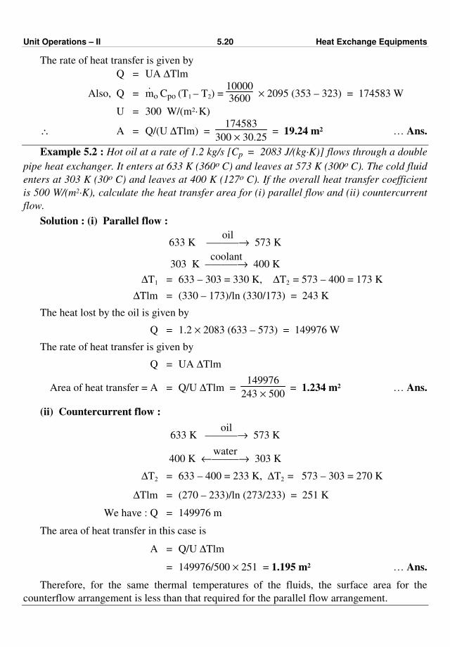
Unit Operations – II 5.20 Heat Exchange Equipments
The rate of heat transfer is given by
Q = UA ∆Tlm
Also, Q = ⋅
mo Cpo (T1 – T2) = 10000
3600 × 2095 (353 – 323) = 174583 W
U = 300 W/(m2·K)
∴ A = Q/(U ∆Tlm) = 174583
300 × 30.25 = 19.24 m2 … Ans.
Example 5.2 : Hot oil at a rate of 1.2 kg/s [Cp = 2083 J/(kg·K)] flows through a double
pipe heat exchanger. It enters at 633 K (360o C) and leaves at 573 K (300o C). The cold fluid
enters at 303 K (30o C) and leaves at 400 K (127o C). If the overall heat transfer coefficient
is 500 W/(m2·K), calculate the heat transfer area for (i) parallel flow and (ii) countercurrent
flow.
Solution : (i) Parallel flow :
633 K oil
––––––→ 573 K
303 K coolant
––––––→ 400 K
∆T1 = 633 – 303 = 330 K, ∆T2 = 573 – 400 = 173 K
∆Tlm = (330 – 173)/ln (330/173) = 243 K
The heat lost by the oil is given by
Q = 1.2 × 2083 (633 – 573) = 149976 W
The rate of heat transfer is given by
Q = UA ∆Tlm
Area of heat transfer = A = Q/U ∆Tlm = 149976
243 × 500 = 1.234 m2 … Ans.
(ii) Countercurrent flow :
633 K oil
––––––→ 573 K
400 K water
←–––––→ 303 K
∆T2 = 633 – 400 = 233 K, ∆T2 = 573 – 303 = 270 K
∆Tlm = (270 – 233)/ln (273/233) = 251 K
We have : Q = 149976 m
The area of heat transfer in this case is
A = Q/U ∆Tlm
= 149976/500 × 251 = 1.195 m2 … Ans.
Therefore, for the same thermal temperatures of the fluids, the surface area for the
counterflow arrangement is less than that required for the parallel flow arrangement.
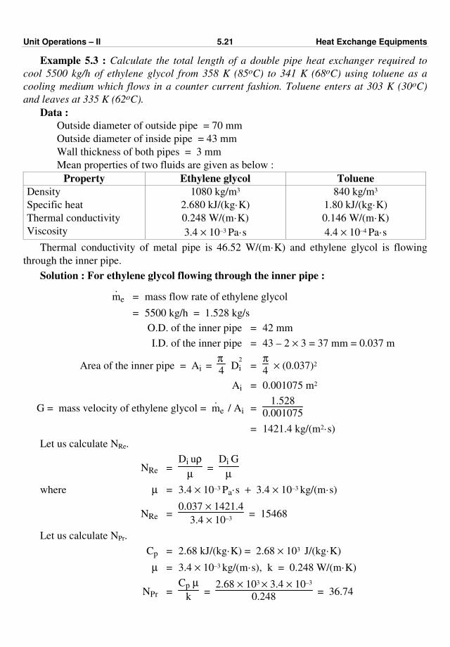
Unit Operations – II 5.21 Heat Exchange Equipments
Example 5.3 : Calculate the total length of a double pipe heat exchanger required to
cool 5500 kg/h of ethylene glycol from 358 K (85oC) to 341 K (68oC) using toluene as a
cooling medium which flows in a counter current fashion. Toluene enters at 303 K (30oC)
and leaves at 335 K (62oC).
Data :
Outside diameter of outside pipe = 70 mm
Outside diameter of inside pipe = 43 mm
Wall thickness of both pipes = 3 mm
Mean properties of two fluids are given as below :
Property Ethylene glycol Toluene
Density
Specific heat
Thermal conductivity
Viscosity
1080 kg/m3
2.680 kJ/(kg·K)
0.248 W/(m·K)
3.4 × 10⁻³ Pa·s
840 kg/m3
1.80 kJ/(kg·K)
0.146 W/(m·K)
4.4 × 10⁻⁴ Pa·s
Thermal conductivity of metal pipe is 46.52 W/(m·K) and ethylene glycol is flowing
through the inner pipe.
Solution : For ethylene glycol flowing through the inner pipe :
⋅
me = mass flow rate of ethylene glycol
= 5500 kg/h = 1.528 kg/s
O.D. of the inner pipe = 42 mm
I.D. of the inner pipe = 43 – 2 × 3 = 37 mm = 0.037 m
Area of the inner pipe = Ai = π 4
D2
i = π4
× (0.037)2
Ai = 0.001075 m2
G = mass velocity of ethylene glycol = ⋅
me / Ai = 1.528
0.001075
= 1421.4 kg/(m2·s)
Let us calculate NRe.
NRe = Di uρ
µ =
Di G
µ
where µ = 3.4 × 10⁻³ Pa·s + 3.4 × 10⁻³ kg/(m·s)
NRe = 0.037 × 1421.4
3.4 × 10–3 = 15468
Let us calculate NPr.
Cp = 2.68 kJ/(kg·K) = 2.68 × 10³ J/(kg·K)
µ = 3.4 × 10⁻³ kg/(m·s), k = 0.248 W/(m·K)
NPr = Cp µ
k =
2.68 × 103 × 3.4 × 10–3
0.248 = 36.74
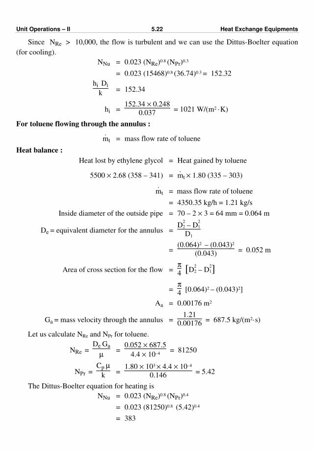
Unit Operations – II 5.22 Heat Exchange Equipments
Since NRe > 10,000, the flow is turbulent and we can use the Dittus-Boelter equation
(for cooling).
NNu = 0.023 (NRe)0.8 (NPr)0.3
= 0.023 (15468)0.8 (36.74)0.3 = 152.32
hi Di
k = 152.34
hi = 152.34 × 0.248
0.037 = 1021 W/(m2 ·K)
For toluene flowing through the annulus :
⋅
mt = mass flow rate of toluene
Heat balance :
Heat lost by ethylene glycol = Heat gained by toluene
5500 × 2.68 (358 – 341) = ⋅
mt × 1.80 (335 – 303)
⋅
mt = mass flow rate of toluene
= 4350.35 kg/h = 1.21 kg/s
Inside diameter of the outside pipe = 70 – 2 × 3 = 64 mm = 0.064 m
De = equivalent diameter for the annulus = D
2
2 – D2
1
D1
= (0.064)2 – (0.043)2
(0.043) = 0.052 m
Area of cross section for the flow = π4
[ ]D2
2 – D2
1
= π4
[0.064)2 – (0.043)2]
Aa = 0.00176 m2
Ga = mass velocity through the annulus = 1.21
0.00176 = 687.5 kg/(m2·s)
Let us calculate NRe and NPr for toluene.
NRe = De Ga
µ =
0.052 × 687.5
4.4 × 10–4 = 81250
NPr = Cp µ
k =
1.80 × 103 × 4.4 × 10–4
0.146 = 5.42
The Dittus-Boelter equation for heating is
NNu = 0.023 (NRe)0.8 (NPr)0.4
= 0.023 (81250)0.8 (5.42)0.4
= 383
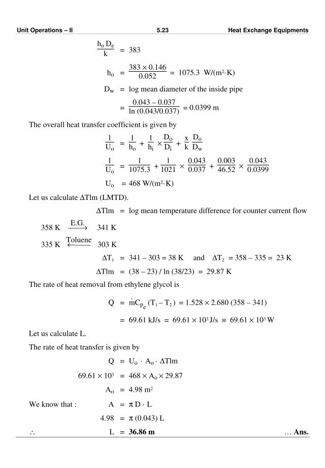
Unit Operations – II 5.23 Heat Exchange Equipments
ho De
k = 383
ho = 383 × 0.146
0.052 = 1075.3 W/(m2·K)
Dw = log mean diameter of the inside pipe
= 0.043 – 0.037
ln (0.043/0.037) = 0.0399 m
The overall heat transfer coefficient is given by
1
Uo =
1
ho +
1
hi ×
Do
Di +
x
k
Do
Dw
1
Uo =
1
1075.3 +
1
1021 ×
0.043
0.037 +
0.003
46.52 ×
0.043
0.0399
Uo = 468 W/(m2·K)
Let us calculate ∆Tlm (LMTD).
∆Tlm = log mean temperature difference for counter current flow
358 K E.G.
–––→ 341 K
335 K Toluene←–––– 303 K
∆T1 = 341 – 303 = 38 K and ∆T2 = 358 – 335 = 23 K
∆Tlm = (38 – 23) / ln (38/23) = 29.87 K
The rate of heat removal from ethylene glycol is
Q = ⋅
mCpe (T1 – T2 ) = 1.528 × 2.680 (358 – 341)
= 69.61 kJ/s = 69.61 × 10³ J/s ≡ 69.61 × 10³ W
Let us calculate L.
The rate of heat transfer is given by
Q = Uo · Ao · ∆Tlm
69.61 × 103 = 468 × Ao × 29.87
Ao = 4.98 m2
We know that : A = π D · L
4.98 = π (0.043) L
∴ L = 36.86 m … Ans.
Unit Operations – II 5.24 Heat Exchange Equipments
EXERCISE
1. Fill in the blanks :
(a) The centre-to-centre distance between baffles is known as baffle ........
Ans. spacing or pitch
(b) The shortest centre-to-centre distance between the adjacent tubes is known as the
........... Ans. tube pitch
(c) The heat transfer equipment which consists of two concentric pipes is called as
............ heat exchanger. Ans. double pipe
(d) External cleaning of the tubes is easy in case of ..... pitch arrangement than
triangular pitch arrangement of tube lay-out. Ans. square
(e) In 1-2 shell and tube heat exchanger the ..... side fluid flows once through
exchanger while ...... side fluid flows twice through exchanger. Ans. shell, tube
(f) For external cleaning of the tubes, tube bundle can be taken out of the shell in a
........ heat exchanger.
(g) The ........ baffles are the drilled plate with heights equal to 75% of the inside
diameter of the shell. Ans. segmental
(h) Kettle reboilers generally incorporates a ......... head arrangement or a ................
arrangement as a heating element. Ans. floating, U-tube
(i) The metal pieces examployed to extend or increase the heat transfer surface are
called................ Ans. fins
(j) In case of .......... fins, long metal strips are attached to the outside of the pipe.
Ans. longitudinal
2. Define the following terms :
(a) condenser (b) cooler (c) vaporiser (d) heater (e) reboiler (f) chiller
3. Give the classification of shell and tube heat exchanger.
4. Explain in brief double pipe heat exchanger.
5. Draw a neat sketch of fixed tube sheet heat exchanger and label its parts.
6. Explain in brief plate heat exchanger.
7. Explain in brief scrapped surface heat exchanger.
8. Draw a neat sketch of kettle reboiler and explain its construction.
9. Draw a neat sketch of floating heat exchanger and explain its construction.
10. What do you mean by the term fins ? Draw neat sketches of longitudinal and
transverse fins.
11. Explain in brief finned tube heat exchanger.
12. Draw a neat sketch of U-tube heat-exchanger and explain briefly its construction.
13. Draw a neat sketch of kettle reboiler and explain in brief its working.
14. Draw a neat sketch of 1-2 shell and tube heat exchanger and label its parts.
15. State the advantages of a floating head heat exchanger.
16. State the advantages of a double pipe heat exchanger and its drawbacks.
ppp
(6.1)
CHAPTER SIX
EVAPORATION
Evaporation is an operation in which a weak solution/liquor is concentrated by
vaporising a portion of the solvent.
The weak liquor/solution to be concentrated is composed of a non-volatile solute and a
volatile solvent.
In this operation, the solvent to be evaporated is generally water and the concentrated
solution/thick liquor is the desired product. The vapour generated usually has no value, it is
condensed and discarded.
It differs from drying in that the residue obtained is a liquid rather than a solid.
It differs from distillation in that the vapour is usually a single component rather than a
mixture of components.
It differs from crystallisation in that the purpose is to concentrate a solution rather than to
form and build crystals.
Evaporation is generally followed by crystallisation and drying.
Evaporation is carried by supplying heat to a solution to vaporise the solvent. The
common heating medium (heat source) is generally a low pressure steam but in some
situations other sources that might be used are : solar energy, fuel, electricity, hot oil and
flue-gas.
In an evaporation operation, heat is utilized to :
(i) increase the temperature of the solution to its boiling point (sensible heat) and
(ii) supply the latent heat of vaporisation of the solvent.
In this operation, rate processes that occur are : heat transfer from a heating medium to a
solution through the solid surface and simultaneous heat and mass transfer from a liquid to a
vapour phase. Irrespective of this, the operation can usually be considered in terms of heat
transfer from a heater to the solution (heat transfer to boiling liquids) for the design of
evaporators.
A wide variation in properties of the solution to be concentrated requires judgement and
experience in the design and operation of evaporators. Some of the properties of evaporating
liquids that have effects on the process of evaporation are :
(i) Concentration : The viscosity and density of the solution increase with increase in
concentration of the solution. The boiling point of the solution increases considerably as the
concentration increases so that it may be much higher than B.P. of water at the same
pressure.
Unit Operations – II 6.2 Evaporation
(ii) Foaming : Some materials have a tendency to foam that causes heavy entrainment
(the carry over of a portion of the liquid by the rising vapour is called an entrainment) and
thus the loss of solution.
(iii) Scale : Some solutions deposit scale on the heat transfer surfaces. This causes
reduction of the heat transfer coefficient and hence the rate of heat transfer. Therefore, it is
necessary to clean the tubes after definite intervals of service.
(iv) Temperature sensitivity : Some materials such as pharmaceuticals and food
products get thermally degraded when heated to moderate temperatures even for short
periods. For concentrating such materials special techniques are to be used which reduce the
temperature of operation and also the time of heating.
(v) Corrosiveness : Whenever contamination and corrosion is a problem, special
materials such as copper, nickel, stainless steels may be used, otherwise mild steel is
normally used for evaporators. Other liquid properties which must be considered in the
design are specific heat, freezing point, toxicity, etc.
The selection of an evaporator for a particular application is based on the analysis of the
factors such as the properties of the solution to be concentrated, operating cost, capacity,
hold-up and residence time. High product viscosity, heat sensitivity, scale formation and
deposition are the major problems that are occurred during the operation of evaporators and
those should be taken into account while designing evaporators for a new installation.
Usually, the desired product of an evaporation operation is the concentrated solution
(thick liquor), but occasionally the evaporated solvent is the primary product as in the
evaporation of sea water to obtain potable water.
Common examples of evaporation are :
Concentration of aqueous solutions of sodium chloride, sodium hydroxide, glycerol,
sugars, milk, fruit juices, etc.
Performance of tubular evaporators :
The performance of a steam heated tubular evaporator is evaluated in terms of
(i) capacity and (ii) economy
Capacity : The capacity of an evaporator is defined as the number of kilogram of water
vaporised / evaporated per hour.
The rate of heat transfer Q, through the heating surface of an evaporator, is defined as the
product of the area of heat transfer surface A, the overall heat transfer coefficient U, and the
overall temperature drop ∆T.
Q = U · A ∆T … (6.1)
where ∆T is the temperature difference between the heating medium and the boiling
solution (saturation temperature of steam minus the boiling point of solution).
Unit Operations – II 6.3 Evaporation
If the feed solution is at the boiling temperature corresponding to the pressure in the
vapour space of an evaporator, then all the heat that is transferred through the heating surface
is available for evaporation (i.e., for converting liquid to vapour) and the capacity is
proportional to the heat transfer rate. If the cold feed solution is fed to the evaporator, heat is
required to increase its temperature to the boiling point and it may be a quite large and thus,
the capacity for a given rate of heat transfer will be reduced accordingly as heat used to
increase the temperature to the boiling point is not available for evaporation. When the feed
solution to the evaporator is at a temperature higher than the boiling point corresponding to
the pressure in the vapour space, a portion of the feed evaporates adiabatically and the
capacity is greater than that corresponding to the heat transfer rate. This process is called
flash evaporation.
Evaporator economy : The economy of an evaporator is defined as the number of
kilogram of water evaporated per kilogram of steam fed to the evaporator. It is also called as
steam economy.
In a single-effect evaporator the amount of water evaporated per kg of steam fed is
always less than one and hence economy is less than one. The fact that the latent heat of
evaporation of water decreases as the pressure increases tends to make the ratio of water
vapour produced, i.e., water evaporated per kg of steam condensed less than unity.
The economy of an evaporator can be increased by reusing the vapour produced.
The methods of increasing the economy are :
(i) use of multiple effect evaporation system
(ii) vapour recompression.
In a multiple effect evaporation system, the vapour produced in the first effect is fed to
the steam chest of the second-effect as a heating medium in which boiling takes place at low
pressure and temperature and so on. Thus in a triple-effect evaporator, 1 kg of steam fed to
the first-effect evaporates approximately 2.5 kg of water.
Another method to increase the economy of an evaporator is to use principle of thermo
compression. Here, the vapour from the evaporator is compressed to increase its temperature
so that it will condense at a temperature higher enough to make possible its use as a heating
medium in the same evaporator.
Boiling point elevation :
In actual practice, the boiling point of a solution is affected by a boiling point elevation
and a liquid head.
As the vapour pressure of most aqueous solutions is less than that of water at any given
temperature, the boiling point of a solution is higher than that of pure water at a given
pressure. The difference between the boiling point of a solution and that of pure water
at any given pressure is known as the boiling point rise/elevation of the solution. The
boiling point elevation is small for dilute solutions and large for concentrated solutions of
inorganic salts.
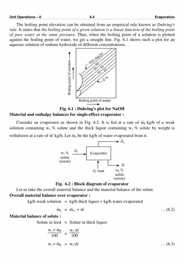
Unit Operations – II 6.4 Evaporation
The boiling point elevation can be obtained from an empirical rule known as Duhring's
rule. It states that the boiling point of a given solution is a linear function of the boiling point
of pure water at the same pressure. Thus, when the boiling point of a solution is plotted
against the boiling point of water, we get a straight line. Fig. 6.1 shows such a plot for an
aqueous solution of sodium hydroxide of different concentrations.
70%NaO
H
60
50 40
30 20
0%
Boili
ng p
oin
t of solu
tion
Boiling point of water
Fig. 6.1 : Duhring's plot for NaOH
Material and enthalpy balances for single-effect evaporator :
Consider an evaporator as shown in Fig. 6.2. It is fed at a rate of ·mf kg/h of a weak
solution containing w1 % solute and the thick liquor containing w2 % solute by weight is
withdrawn at a rate of ·m' kg/h. Let
·mv be the kg/h of water evaporated from it.
w %
solids1
(solute)
Q. heat w %
solids(solute)
2
mv
m'
mf Evaporator
Fig. 6.2 : Block diagram of evaporator
Let us take the overall material balance and the material balance of the solute.
Overall material balance over evaporator :
kg/h weak solution = kg/h thick liquor + kg/h water evaporated
·mf = ·mv + ·m' … (6.2)
Material balance of solute :
Solute in feed = Solute in thick liquor
w1 × ·mf
100 =
w2 ·m'
100
w1 × ·mf = w2 ·m' … (6.3)
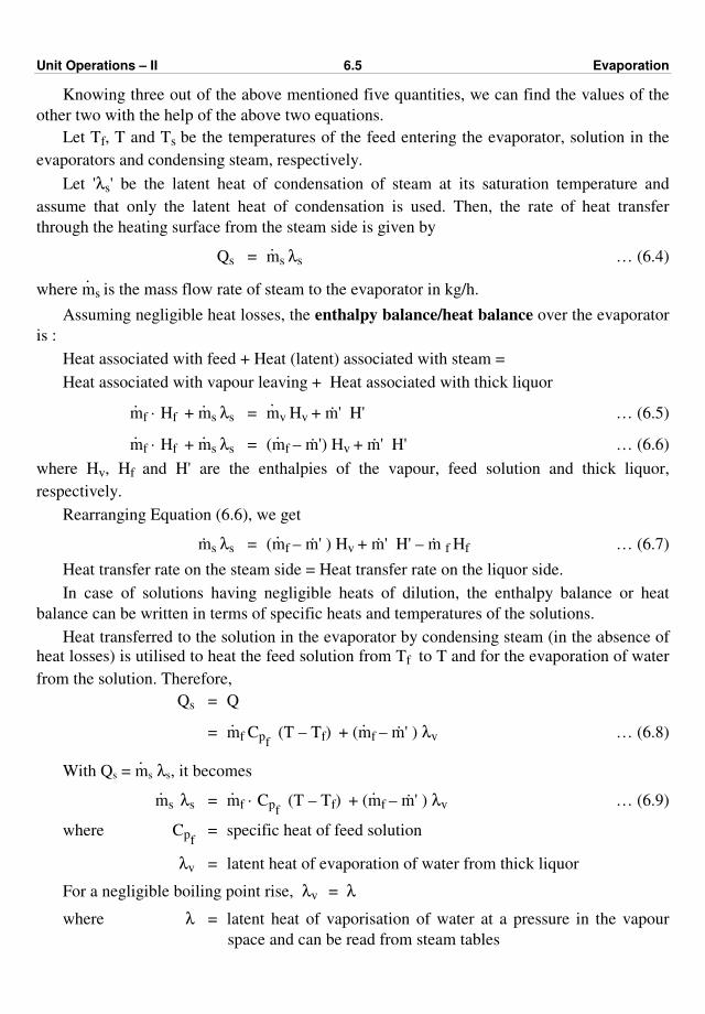
Unit Operations – II 6.5 Evaporation
Knowing three out of the above mentioned five quantities, we can find the values of the
other two with the help of the above two equations.
Let Tf, T and Ts be the temperatures of the feed entering the evaporator, solution in the
evaporators and condensing steam, respectively.
Let 'λs' be the latent heat of condensation of steam at its saturation temperature and
assume that only the latent heat of condensation is used. Then, the rate of heat transfer
through the heating surface from the steam side is given by
Qs = ·ms λs … (6.4)
where ·ms is the mass flow rate of steam to the evaporator in kg/h.
Assuming negligible heat losses, the enthalpy balance/heat balance over the evaporator
is :
Heat associated with feed + Heat (latent) associated with steam =
Heat associated with vapour leaving + Heat associated with thick liquor
·mf · Hf + ·ms λs = ·mv Hv + ·m' H' … (6.5)
·mf · Hf + ·ms λs = ( ·mf – ·m') Hv + ·m' H' … (6.6)
where Hv, Hf and H' are the enthalpies of the vapour, feed solution and thick liquor,
respectively.
Rearranging Equation (6.6), we get
·ms λs = ( ·mf – ·m' ) Hv + ·m' H' – ·m f Hf … (6.7)
Heat transfer rate on the steam side = Heat transfer rate on the liquor side.
In case of solutions having negligible heats of dilution, the enthalpy balance or heat
balance can be written in terms of specific heats and temperatures of the solutions.
Heat transferred to the solution in the evaporator by condensing steam (in the absence of
heat losses) is utilised to heat the feed solution from Tf to T and for the evaporation of water
from the solution. Therefore,
Qs = Q
= ·mf Cpf (T – Tf) + ( ·mf – ·m' ) λv … (6.8)
With Qs = ·ms λs, it becomes
·ms λs = ·mf · Cpf (T – Tf) + ( ·mf – ·m' ) λv … (6.9)
where Cpf = specific heat of feed solution
λv = latent heat of evaporation of water from thick liquor
For a negligible boiling point rise, λv = λ
where λ = latent heat of vaporisation of water at a pressure in the vapour
space and can be read from steam tables
Unit Operations – II 6.6 Evaporation
With this Equation (6.9) becomes
·ms λs = ·mf Cpf (T – Tf) + ( ·mf – ·m' ) λ … (6.10)
·ms λs = ·mf · Cpf (T – Tf) + ·m λ … (6.11)
The boiling point of a solution (T) corresponding to a pressure in the vapour space can be
obtained by knowing the boiling point elevation and boiling point of pure water at that
pressure, e.g. if T' is the boiling point of water at a certain pressure of the operation and 'P' is
the boiling point elevation, then
T = T' + P
The heat transfer surface/area of an evaporator is calculated with the help of the
following equation :
Q = U · A · ∆T … (6.12)
Q = ·ms λs = U · A · ∆T … (6.13)
where U = overall heat transfer coefficient
A = area of heat transfer
and ∆T = temperature difference
∆T = Ts – T
∆T = Condensing steam temperature – Boiling point of solution
When 'Q' is in W, 'U' is in W/(m2·K) and '∆T' is in K, then 'A' will be in m2.
λs = Specific enthalpy of saturated steam
– Specific enthalpy of saturated water (i.e., of condensate)
Evaporator Types :
Evaporators used in the chemical process industries can be classified as :
(i) Natural circulation evaporators.
(ii) Forced circulation evaporators.
Natural circulation evaporators are commonly used for simpler evaporation operations
singly or in multiple effect, e.g., horizontal tube evaporator, vertical tube evaporator etc.,
whereas forced circulation evaporators are commonly used for salting, viscous and scale
forming solutions. The forced circulation units may be provided with an external horizontal
or vertical heating element.
Open pan evaporator / Jacketed pan evaporator :
The simplest method of concentrating a solution makes use of jacketed pans. Such a type
of evaporator is particularly suitable when small quantities are to be handled. In an
open/jacketed pan evaporator, condensing steam is fed to a jacket for evaporating a part of
the solvent.

Unit Operations – II 6.7 Evaporation
Steam
JacketCondensate
Pan
Product Fig. 6.3 : Jacketed pan evaporator
Pan is made of a single sheet of metal (for small sizes) or several sheets joined by
welding / brazing. A jacket is welded to the pan. The jacket is provided with a steam inlet at
the top, while a condensate drain is provided at its bottom. The pan is provided with an outlet
at the bottom for draining its contents. The jacket is usually constructed out of mild steel,
while the pan is constructed out of mild steel, stainless steel, copper or aluminium as per
process requirements.
The solution to be concentrated is taken into the pan and steam is admitted in the jacket.
Evaporation is carried out for a predetermined time to achieve a desired concentration level.
The thick liquor is then drained from the outlet.
Horizontal tube evaporator : It consists of a vertical cylindrical shell incorporating a horizontal square tube bundle at the lower portion of the shell. Channels are provided on either ends of the tube bundle for introduction of steam and withdrawal of condensate. The shell is closed by dished heads at both the ends. A vapour outlet is provided on the top cover and a thick liquor outlet is provided at the bottom. Feed point is located at a convenient point. In this evaporator, steam is inside the tube and the liquor to be concentrated surrounds the tubes. Steam which is admitted through one of the steam chests/channels and flows through the tubes. Steam gets condensed by transferring its latent heat and the condensate is removed from the outlet provided at the bottom of the opposite steam chest. This type of evaporator is shown in Fig. 6.4.
Feed
Condensate
Thick liquor
Steam
Vapour
Steam chest
Tube
Evaporator body
Fig. 6.4 : Horizontal tube evaporator
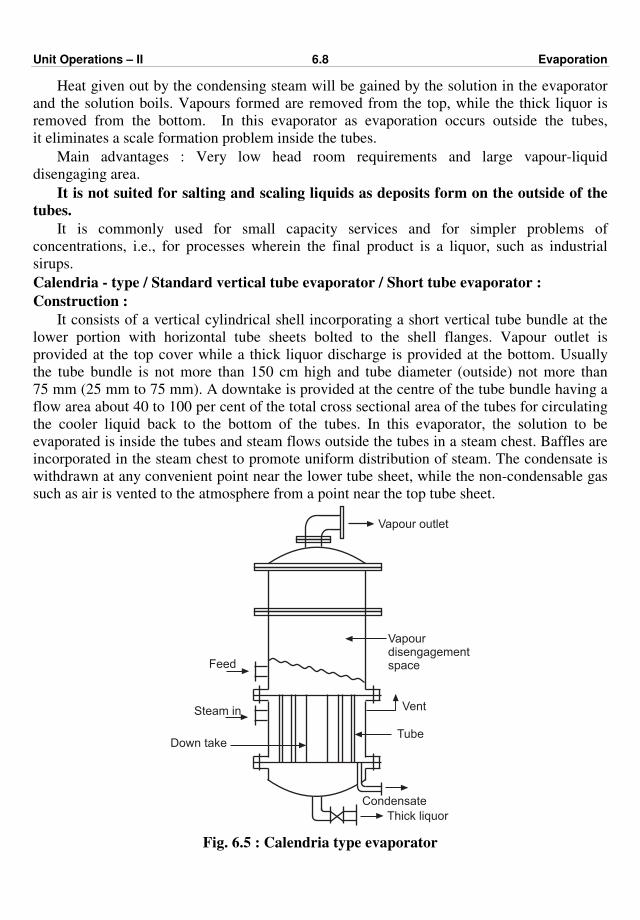
Unit Operations – II 6.8 Evaporation
Heat given out by the condensing steam will be gained by the solution in the evaporator
and the solution boils. Vapours formed are removed from the top, while the thick liquor is
removed from the bottom. In this evaporator as evaporation occurs outside the tubes,
it eliminates a scale formation problem inside the tubes.
Main advantages : Very low head room requirements and large vapour-liquid
disengaging area.
It is not suited for salting and scaling liquids as deposits form on the outside of the
tubes.
It is commonly used for small capacity services and for simpler problems of
concentrations, i.e., for processes wherein the final product is a liquor, such as industrial
sirups.
Calendria - type / Standard vertical tube evaporator / Short tube evaporator :
Construction :
It consists of a vertical cylindrical shell incorporating a short vertical tube bundle at the
lower portion with horizontal tube sheets bolted to the shell flanges. Vapour outlet is
provided at the top cover while a thick liquor discharge is provided at the bottom. Usually
the tube bundle is not more than 150 cm high and tube diameter (outside) not more than
75 mm (25 mm to 75 mm). A downtake is provided at the centre of the tube bundle having a
flow area about 40 to 100 per cent of the total cross sectional area of the tubes for circulating
the cooler liquid back to the bottom of the tubes. In this evaporator, the solution to be
evaporated is inside the tubes and steam flows outside the tubes in a steam chest. Baffles are
incorporated in the steam chest to promote uniform distribution of steam. The condensate is
withdrawn at any convenient point near the lower tube sheet, while the non-condensable gas
such as air is vented to the atmosphere from a point near the top tube sheet.
Vapour outlet
Vapourdisengagementspace
Vent
TubeDown take
Steam in
Feed
Condensate
Thick liquor
Fig. 6.5 : Calendria type evaporator
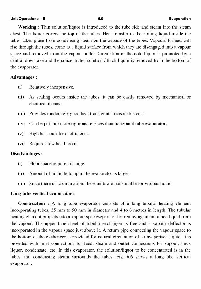
Unit Operations – II 6.9 Evaporation
Working : Thin solution/liquor is introduced to the tube side and steam into the steam
chest. The liquor covers the top of the tubes. Heat transfer to the boiling liquid inside the
tubes takes place from condensing steam on the outside of the tubes. Vapours formed will
rise through the tubes, come to a liquid surface from which they are disengaged into a vapour
space and removed from the vapour outlet. Circulation of the cold liquor is promoted by a
central downtake and the concentrated solution / thick liquor is removed from the bottom of
the evaporator.
Advantages :
(i) Relatively inexpensive.
(ii) As scaling occurs inside the tubes, it can be easily removed by mechanical or
chemical means.
(iii) Provides moderately good heat transfer at a reasonable cost.
(iv) Can be put into more rigorous services than horizontal tube evaporators.
(v) High heat transfer coefficients.
(vi) Requires low head room.
Disadvantages :
(i) Floor space required is large.
(ii) Amount of liquid hold up in the evaporator is large.
(iii) Since there is no circulation, these units are not suitable for viscous liquid.
Long tube vertical evaporator :
Construction : A long tube evaporator consists of a long tubular heating element
incorporating tubes, 25 mm to 50 mm in diameter and 4 to 8 metres in length. The tubular
heating element projects into a vapour space/separator for removing an entrained liquid from
the vapour. The upper tube sheet of tubular exchanger is free and a vapour deflector is
incorporated in the vapour space just above it. A return pipe connecting the vapour space to
the bottom of the exchanger is provided for natural circulation of a unvaporised liquid. It is
provided with inlet connections for feed, steam and outlet connections for vapour, thick
liquor, condensate, etc. In this evaporator, the solution/liquor to be concentrated is in the
tubes and condensing steam surrounds the tubes. Fig. 6.6 shows a long-tube vertical
evaporator.

Unit Operations – II 6.10 Evaporation
Thickliquor
Na
tura
l circu
latio
no
f u
ne
va
po
rate
dliq
uidSteam
Heatingelement
Tube
Condensate
Feed
Deflector
Vapour space
Vapour outlet
Fig. 6.6 : Long-tube vertical evaporator
Working :
In this evaporator, feed enters the bottom of the tubes, gets heated by the condensing
steam, starts to boil part way up the tubes and a mixture of vapour and liquid issues from the
top of tubes and finally impinges at a high velocity on a deflector. The deflector acts both as
a primary separator and a foam breaker. Some part of the separated liquid is removed as a
product and the remaining part is returned to the bottom of the evaporator.
This type of evaporator is widely used for handling of foamy, frothy liquors.
It is used for the production of condensed milk and concentrating a black liquor in the
pulp and paper industry.
Forced Circulation Evaporators :
Whenever we are dealing with concentration problems involving solutions of high
viscosities or of scale forming tendencies we have to make use of forced circulation
evaporators as increasing the velocity of flow of liquor through tubes increases remarkably
the liquid film heat transfer coefficients and the high velocity resulting by use of a centrifugal
pump prevents the formation of excessive deposits on the heat transfer surfaces. In a natural
circulation evaporator, the liquid enters the tube at a velocity of 0.3 to 1 metre per second,
whereas in a forced circulation evaporator, the velocity is of the order of 2 to 6 metres per
second. In the forced circulation evaporator, smaller diameter tubes are used compared to
those in the natural circulation evaporator, generally not larger than 50 mm.
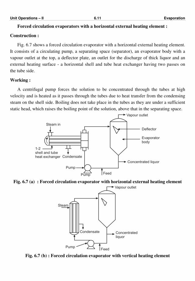
Unit Operations – II 6.11 Evaporation
Forced circulation evaporators with a horizontal external heating element :
Construction :
Fig. 6.7 shows a forced circulation evaporator with a horizontal external heating element.
It consists of a circulating pump, a separating space (separator), an evaporator body with a
vapour outlet at the top, a deflector plate, an outlet for the discharge of thick liquor and an
external heating surface - a horizontal shell and tube heat exchanger having two passes on
the tube side.
Working :
A centrifugal pump forces the solution to be concentrated through the tubes at high
velocity and is heated as it passes through the tubes due to heat transfer from the condensing
steam on the shell side. Boiling does not take place in the tubes as they are under a sufficient
static head, which raises the boiling point of the solution, above that in the separating space.
Steam in
Vapour outlet
Concentrated liquor
FeedPump
Condensate
1-2shell and tubeheat exchanger
Pump
Deflector
Evaporatorbody
Fig. 6.7 (a) : Forced circulation evaporator with horizontal external heating element
Condensate
Steam
Vapour outlet
Concentratedliquor
FeedPump
Fig. 6.7 (b) : Forced circulation evaporator with vertical heating element
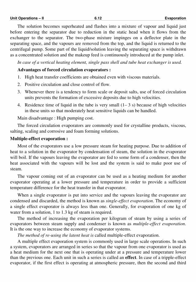
Unit Operations – II 6.12 Evaporation
The solution becomes superheated and flashes into a mixture of vapour and liquid just
before entering the separator due to reduction in the static head when it flows from the
exchanger to the separator. The two-phase mixture impinges on a deflector plate in the
separating space, and the vapours are removed from the top, and the liquid is returned to the
centrifugal pump. Some part of the liquid/solution leaving the separating space is withdrawn
as a concentrated solution and the makeup feed is continuously introduced at the pump inlet.
In case of a vertical heating element, single pass shell and tube heat exchanger is used.
Advantages of forced circulation evaporators :
1. High heat transfer coefficients are obtained even with viscous materials.
2. Positive circulation and close control of flow.
3. Whenever there is a tendency to form scale or deposit salts, use of forced circulation
units prevents the formation of excessive deposits due to high velocities.
4. Residence time of liquid in the tube is very small (1– 3 s) because of high velocities
in these units so that moderately heat sensitive liquids can be handled.
Main disadvantage : High pumping cost.
The forced circulation evaporators are commonly used for crystalline products, viscous,
salting, scaling and corrosive and foam forming solutions.
Multiple-effect evaporation :
Most of the evaporators use a low pressure steam for heating purpose. Due to addition of
heat to a solution in the evaporator by condensation of steam, the solution in the evaporator
will boil. If the vapours leaving the evaporator are fed to some form of a condenser, then the
heat associated with the vapours will be lost and the system is said to make poor use of
steam.
The vapour coming out of an evaporator can be used as a heating medium for another
evaporator operating at a lower pressure and temperature in order to provide a sufficient
temperature difference for the heat transfer in that evaporator.
When a single evaporator is put into service and the vapours leaving the evaporator are
condensed and discarded, the method is known as single-effect evaporation. The economy of
a single effect evaporator is always less than one. Generally, for evaporation of one kg of
water from a solution, 1 to 1.3 kg of steam is required.
The method of increasing the evaporation per kilogram of steam by using a series of
evaporators between steam supply and condenser is known as multiple-effect evaporation.
It is the one way to increase the economy of evaporator systems.
The method of re-using the latent heat is called multiple-effect evaporation.
A multiple effect evaporation system is commonly used in large scale operations. In such
a system, evaporators are arranged in series so that the vapour from one evaporator is used as
a heat medium for the next one that is operating under at a pressure and temperature lower
than the previous one. Each unit in such a series is called an effect. In case of a tripple-effect
evaporator, if the first effect is operating at atmospheric pressure, then the second and third
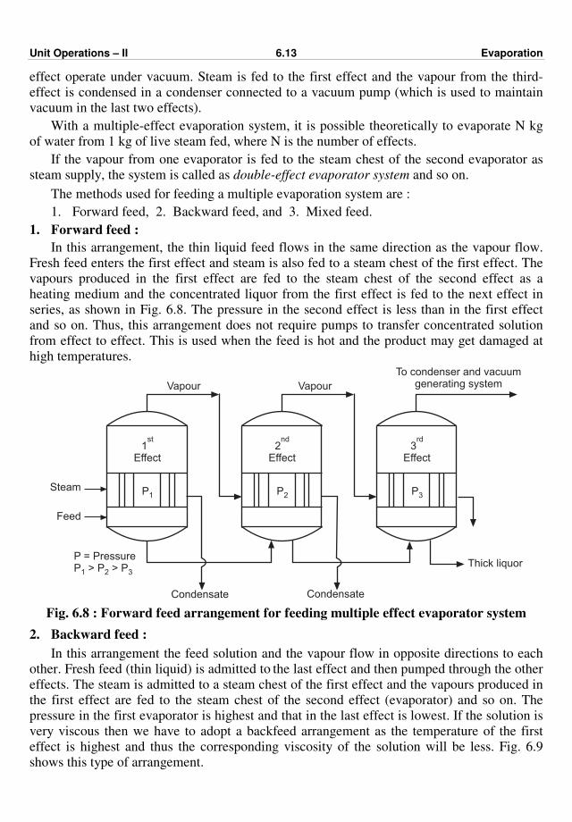
Unit Operations – II 6.13 Evaporation
effect operate under vacuum. Steam is fed to the first effect and the vapour from the third-
effect is condensed in a condenser connected to a vacuum pump (which is used to maintain
vacuum in the last two effects).
With a multiple-effect evaporation system, it is possible theoretically to evaporate N kg
of water from 1 kg of live steam fed, where N is the number of effects.
If the vapour from one evaporator is fed to the steam chest of the second evaporator as
steam supply, the system is called as double-effect evaporator system and so on.
The methods used for feeding a multiple evaporation system are :
1. Forward feed, 2. Backward feed, and 3. Mixed feed.
1. Forward feed :
In this arrangement, the thin liquid feed flows in the same direction as the vapour flow.
Fresh feed enters the first effect and steam is also fed to a steam chest of the first effect. The
vapours produced in the first effect are fed to the steam chest of the second effect as a
heating medium and the concentrated liquor from the first effect is fed to the next effect in
series, as shown in Fig. 6.8. The pressure in the second effect is less than in the first effect
and so on. Thus, this arrangement does not require pumps to transfer concentrated solution
from effect to effect. This is used when the feed is hot and the product may get damaged at
high temperatures.
Steam
Feed
1Effect
st
P1
Vapour
2Effect
nd
P2
3Effect
rd
P3
Vapour
To condenser and vacuumgenerating system
P = PressureP > P > P1 2 3
Condensate Condensate
Thick liquor
Fig. 6.8 : Forward feed arrangement for feeding multiple effect evaporator system
2. Backward feed :
In this arrangement the feed solution and the vapour flow in opposite directions to each
other. Fresh feed (thin liquid) is admitted to the last effect and then pumped through the other
effects. The steam is admitted to a steam chest of the first effect and the vapours produced in
the first effect are fed to the steam chest of the second effect (evaporator) and so on. The
pressure in the first evaporator is highest and that in the last effect is lowest. If the solution is
very viscous then we have to adopt a backfeed arrangement as the temperature of the first
effect is highest and thus the corresponding viscosity of the solution will be less. Fig. 6.9
shows this type of arrangement.
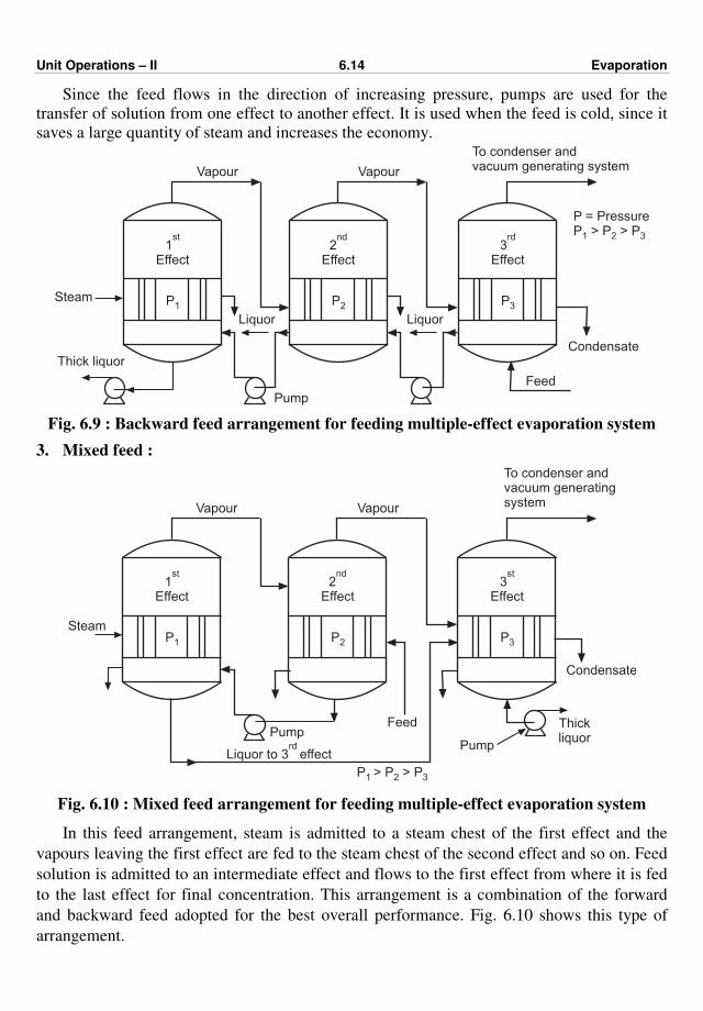
Unit Operations – II 6.14 Evaporation
Since the feed flows in the direction of increasing pressure, pumps are used for the
transfer of solution from one effect to another effect. It is used when the feed is cold, since it
saves a large quantity of steam and increases the economy.
Steam
Thick liquor
1Effect
st
P1
Vapour
2Effect
nd
P2
3Effect
rd
P3
Vapour
To condenser andvacuum generating system
Pump
Liquor Liquor
Feed
Condensate
P = PressureP > P > P1 2 3
Fig. 6.9 : Backward feed arrangement for feeding multiple-effect evaporation system
3. Mixed feed :
Steam
1Effect
st
P1
Vapour
2Effect
nd
P2
3Effect
st
P3
Vapour
To condenser andvacuum generatingsystem
Pump
Liquor to 3rd
effect
Thickliquor
Pump
Feed
P P P1 2 3> >
Condensate
Fig. 6.10 : Mixed feed arrangement for feeding multiple-effect evaporation system
In this feed arrangement, steam is admitted to a steam chest of the first effect and the
vapours leaving the first effect are fed to the steam chest of the second effect and so on. Feed
solution is admitted to an intermediate effect and flows to the first effect from where it is fed
to the last effect for final concentration. This arrangement is a combination of the forward
and backward feed adopted for the best overall performance. Fig. 6.10 shows this type of
arrangement.

Unit Operations – II 6.15 Evaporation
Comparison of forward feed and backward feed arrangements :
1. In the forward feed, the flow of the solution to be concentrated is parallel to the
steam/vapour flow.
1. In the backward feed, the flow of the solution to be concentrated is in opposite
direction to that of steam/vapour (counter current).
2. Forward feed arrangement does not need pumps for moving the solution from effect
to effect as vacuum is maintained in the last effect.
2. Backward feed arrangement needs pumps for moving the solution from effect to
effect as transfer of the solution is to be done from the evaporator operating at a low
pressure to that operating at a higher pressure.
3. In the forward feed as heating of the cold feed solution is done in the first effect, less
vapour is produced per kilograms of steam fed, resulting into a lower economy.
3. In the backward feed, the solution is heated in each effect which usually results in a
better economy than that with a forward feed.
4. With a forward feed, the most concentrated solution is in the last effect wherein the
temperature is the lowest and the viscosity is the highest. These conditions lead to
reduction in the capacity of the system as a whole due to low overall coefficient in
the last effect in case of thick liquors which are very viscous.
4. In the case of backward feed, the concentrated solution is in the first effect wherein
the temperature is the highest as steam is admitted to that effect and the viscosity is
the lowest, thus the overall coefficient can be moderately high inspite of high
viscosity.
5. In the case of forward feed, the maintenance charges and power cost are less.
5. In the case of backward feed, the maintenance charges and power cost are more for
the same duty.
6. The forward feed arrangement is less effective thermally.
6. The backward feed arrangement is more effective thermally. (At high feed
temperatures).
7. Forward feed is more economical in steam.
7. At low values of feed temperature, backward feed arrangement gives higher
economy.
8. Forward feed is very common (largely used) as it is simple to operate.
8. Backward feed is not common as it necessitates the use of pump between effects.
The choice of optimum number of effects will be determined by an economic balance
between the savings in steam obtained by using a multiple-effect evaporation system and the
additional investment cost resulting from the added heat transfer area.
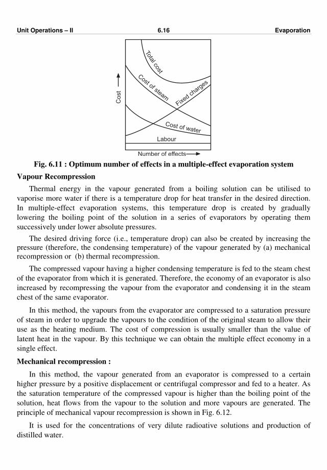
Unit Operations – II 6.16 Evaporation
Total cost
Cost of steam
Fixed
charg
es
Cost
Cost of water
Labour
Number of effects
Fig. 6.11 : Optimum number of effects in a multiple-effect evaporation system
Vapour Recompression
Thermal energy in the vapour generated from a boiling solution can be utilised to
vaporise more water if there is a temperature drop for heat transfer in the desired direction.
In multiple-effect evaporation systems, this temperature drop is created by gradually
lowering the boiling point of the solution in a series of evaporators by operating them
successively under lower absolute pressures.
The desired driving force (i.e., temperature drop) can also be created by increasing the
pressure (therefore, the condensing temperature) of the vapour generated by (a) mechanical
recompression or (b) thermal recompression.
The compressed vapour having a higher condensing temperature is fed to the steam chest
of the evaporator from which it is generated. Therefore, the economy of an evaporator is also
increased by recompressing the vapour from the evaporator and condensing it in the steam
chest of the same evaporator.
In this method, the vapours from the evaporator are compressed to a saturation pressure
of steam in order to upgrade the vapours to the condition of the original steam to allow their
use as the heating medium. The cost of compression is usually smaller than the value of
latent heat in the vapour. By this technique we can obtain the multiple effect economy in a
single effect.
Mechanical recompression :
In this method, the vapour generated from an evaporator is compressed to a certain
higher pressure by a positive displacement or centrifugal compressor and fed to a heater. As
the saturation temperature of the compressed vapour is higher than the boiling point of the
solution, heat flows from the vapour to the solution and more vapours are generated. The
principle of mechanical vapour recompression is shown in Fig. 6.12.
It is used for the concentrations of very dilute radioative solutions and production of
distilled water.
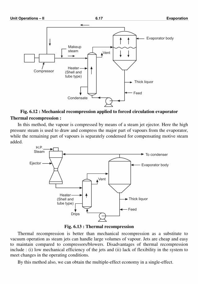
Unit Operations – II 6.17 Evaporation
Condensate
Heater(Shell andtube type)
Vent
Makeupsteam
Compressor
Thick liquor
Feed
Evaporator body
Fig. 6.12 : Mechanical recompression applied to forced circulation evaporator
Thermal recompression :
In this method, the vapour is compressed by means of a steam jet ejector. Here the high
pressure steam is used to draw and compress the major part of vapours from the evaporator,
while the remaining part of vapours is separately condensed for compensating motive steam
added.
H.P.Steam
Ejector
Heater(Shell andtube type)
Drips
Vent
Thick liquor
Feed
Evaporator body
To condenser
Fig. 6.13 : Thermal recompression
Thermal recompression is better than mechanical recompression as a substitute to
vacuum operation as steam jets can handle large volumes of vapour. Jets are cheap and easy
to maintain compared to compressors/blowers. Disadvantages of thermal recompression
include : (i) low mechanical efficiency of the jets and (ii) lack of flexibility in the system to
meet changes in the operating conditions.
By this method also, we can obtain the multiple-effect economy in a single-effect.

Unit Operations – II 6.18 Evaporation
Choice of steam pressure : In any evaporation operation, generally, a low pressure steam is used. We cannot use a
high pressure steam that gives a larger temperature drop that consequently decrease the size
and therefore the cost of the evaporator, since it is much more valuable as a source of power
than as a source of heat. High pressure steam has a lower latent heat than a low pressure
steam and hence the low pressure steam delivers more latent heat than the high pressure
steam for evaporation of the solvent. Also the construction of the evaporator to hold the high
pressure steam would be much more expensive (since it demands heavy thickness) than the
construction to hold the low pressure steam.
Pressure in the vapour space : It is always desirable to have a larger temperature drop between the condensing steam
and the boiling point of a solution because as the temperature drop increases, the heating
surface and in turn the cost of the evaporator decreases. By making use of a condenser and a
vacuum pump, the pressure in the vapour space of the evaporator is made less than
atmospheric. So by operating the evaporator at a pressure less than atmospheric, i.e.,
operating under a vacuum results in decrease in the boiling point of the solution which in
turn leads to a larger value of temperature drop that decreases the required heat transfer
surface.
It is not necessary to operate the evaporators under vacuum, but as it is economical to
feed them with steam at a relatively moderate pressure, a vacuum is necessary in order to get
an economical temperature drop (∆T). There are certain cases where the operation under
vacuum is necessary, for example, while dealing with heat sensitive materials (they may get
decomposed/degraded if boiled at higher temperatures). Evaporators operating at high
pressures requires much more expensive construction than when operating at lower
pressures. Basically evaporators are operated under vacuum to obtain a larger temperature
drop (∆T).
Evaporator accessories : These are devices that must be supplied with every evaporator.
(i) condensers (ii) vacuum pump / steam jet ejector.
There are two types of condensers :
(i) Surface condensers and (ii) Contact condensers : parallel current, counter current etc.
In a surface condenser, the vapour to be condensed and the cooling medium are separated
by a metal wall, whereas in a contact condenser the vapour and the cooling medium/liquid
are mixed directly.
Parallel-current condenser : It is the one in which the non-condensed gases leave at a
temperature of the exit cooling water.
Counter-current condenser : It is the one in which the non-condensed gases leave at a
temperature of the entering cooling water.
Wet condenser : It is the one in which the non-condensed gases and cooling water are
removed by the same pump.
Dry condenser : It is the one in which the non-condensed gases and cooling water are
removed by separate pumps.
Barometric condenser : It is the one that is placed high enough so that water escape
from it by a barometric leg.
Low level condenser : It is the one in which water is removed by a pump.

Unit Operations – II 6.19 Evaporation
In practice parallel current condensers are almost always wet condensers, while counter-
current condensers are always dry.
Materials of construction for evaporators : Evaporator bodies are generally fabricated
from mild steel as it is least expensive and easy to fabricate. For corrosive solutions,
materials like monel, inconel and stainless steel are used. The tubes are made of copper,
stainless steel and the tube sheet may be of cast bronze, nickel clad steel or stainless steel.
SOLVED EXAMPLES
Example 6.1 : Calculate the boiling point elevation of a solution and the driving force
for heat transfer using the following data :
Data : Solution boils at a temperature of 380 K (107 oC) and the boiling point of water
at a pressure in the vapour space is 373 K (100 oC)
Temperature of condensing steam is 399 K (126o C).
Solution : Boiling point of the solution = T = 380 K
Boiling point of water = T' = 373 K
Boiling point elevation = T – T' = 380 – 373 K
= 7 K (or oC) … Ans.
Saturation temperature of the condensing steam = Ts = 399 K
Driving force for heat transfer = Ts – T = 399 – 380
= 19 K … Ans.
Note : Whenever the pressure at which steam is available and pressure prevailing in the
vapour space of an evaporator are given, then the steam table should be referred to find the
temperature of steam, latent heat of condensation of steam based on a given steam pressure
and the latent heat of evaporation of water, i.e., latent heat of vapour based on a pressure
prevailing in the vapour space of the evaporator.
Example 6.2 : An evaporator operating at atmospheric pressure (101.325 kPa) is fed at
the rate of 10000 kg/h of weak liquor containing 4 % caustic soda. Thick liquor leaving the
evaporator contains 25% caustic soda. Find the capacity of the evaporator.
Solution :
Basis : 10,000 kg/h of weak liquor entering the evaporator.
Let .
m' be the kg/h of thick liquor leaving the evaporator.
Material balance of caustic soda :
Caustic soda in the feed = Caustic soda in the thick liquor
0.04 × 10000 = 0.25 × .
m'
.
m' = 1600 kg/h
Overall material balance :
kg/h of feed = kg/h water evaporated + kg/h of thick liquor
10000 = kg/h water evaporated + 1600
water evaporated = 10000 – 1600 = 8400 kg/h
∴ Capacity of the evaporator = 8400 kg/h … Ans.
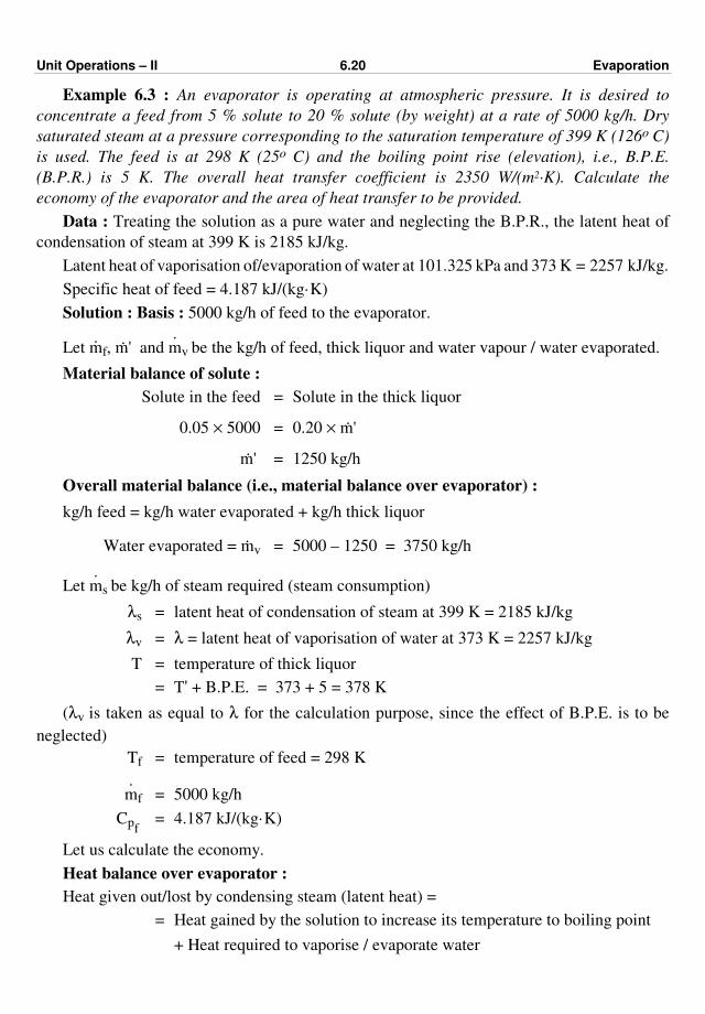
Unit Operations – II 6.20 Evaporation
Example 6.3 : An evaporator is operating at atmospheric pressure. It is desired to
concentrate a feed from 5 % solute to 20 % solute (by weight) at a rate of 5000 kg/h. Dry
saturated steam at a pressure corresponding to the saturation temperature of 399 K (126o C)
is used. The feed is at 298 K (25o C) and the boiling point rise (elevation), i.e., B.P.E.
(B.P.R.) is 5 K. The overall heat transfer coefficient is 2350 W/(m2·K). Calculate the
economy of the evaporator and the area of heat transfer to be provided.
Data : Treating the solution as a pure water and neglecting the B.P.R., the latent heat of
condensation of steam at 399 K is 2185 kJ/kg.
Latent heat of vaporisation of/evaporation of water at 101.325 kPa and 373 K = 2257 kJ/kg.
Specific heat of feed = 4.187 kJ/(kg·K)
Solution : Basis : 5000 kg/h of feed to the evaporator.
Let .
mf, .
m' and ⋅
mv be the kg/h of feed, thick liquor and water vapour / water evaporated.
Material balance of solute :
Solute in the feed = Solute in the thick liquor
0.05 × 5000 = 0.20 × .
m'
.
m' = 1250 kg/h
Overall material balance (i.e., material balance over evaporator) :
kg/h feed = kg/h water evaporated + kg/h thick liquor
Water evaporated = .
mv = 5000 – 1250 = 3750 kg/h
Let ⋅
ms be kg/h of steam required (steam consumption)
λs = latent heat of condensation of steam at 399 K = 2185 kJ/kg
λv = λ = latent heat of vaporisation of water at 373 K = 2257 kJ/kg
T = temperature of thick liquor
= T' + B.P.E. = 373 + 5 = 378 K
(λv is taken as equal to λ for the calculation purpose, since the effect of B.P.E. is to be
neglected)
Tf = temperature of feed = 298 K
⋅
mf = 5000 kg/h
Cpf = 4.187 kJ/(kg·K)
Let us calculate the economy.
Heat balance over evaporator :
Heat given out/lost by condensing steam (latent heat) =
= Heat gained by the solution to increase its temperature to boiling point
+ Heat required to vaporise / evaporate water
Unit Operations – II 6.21 Evaporation
⋅
ms λs = ⋅
mf Cpf (T – Tf) + ·mv λ
⋅
ms × 2185 = 5000 × 4.187 (378 – 298) + 3750 × 2257
⋅
ms = 4640.1 kg/h
Steam consumption = 4640.1 kg/h
Economy of the evaporator = kg/h water evaporated
kg/h steam consumed
= 3750
4640.1 = 0.808
kg evaporation
kg steam … Ans.
Let us calculate the heat transfer area.
Rate of heat transfer = Q = ⋅
ms λs
= 4640.1 × 2185
= 10138619 kJ/kg
= 10138619 × 1000
3600
= 2816283 J/s ≡ 2816283 W
Ts = saturation temperature of steam = 399 K
Temperature driving force = ∆T = Ts – T
= 399 – 378
= 21 K (21o C)
U = 2350 W/(m2·K)
We have : Q = UA ∆T
∴ A = Q/U ∆T = 2816283 / (2350 × 21)
= 57.07 m2
Heat transfer area to be provided = 57.07 m2 … Ans.
Example 6.4 : A solution containing 10 % solids is to be concentrated to a level of
50 % solids. Steam is available at a pressure of 0.20 MPa [saturation temperature of
393 K (120o C)]. Feed rate to the evaporator is 30000 kg/h. The evaporator is working at
reduced pressure such that boiling point is 323 K (50o C). The overall heat transfer
coefficient is 2.9 kW/(m2·K). Estimate the steam economy and heat transfer surface for :
(i) Feed introduced at 293 K (20o C)
(ii) Feed introduced at 308 K (35o C).
Data : Specific heat of feed = 3.98 kJ/(kg·K)
Latent heat of condensation of steam at 0.20 MPa = 2202 kJ/kg
Latent heat of vaporisation of water at 323 K (i.e. at pressure in the vapour space
= 2383 kJ/kg).
Unit Operations – II 6.22 Evaporation
Solution : Basis : 30000 kg/h feed to the evaporator.
Let ·mf, ·m' and ·mv be the mass flow rate of feed, thick liquor and water vapour
respectively.
Material balance of solids :
Solids in the feed = Solids in the thick liquor
0.10 × 30000 = 0.05 ·m'
·m' = 6000 kg/h
Overall material balance :
kg/h feed = kg/h water evaporated + kg/h thick liquor
Water evaporated = ⋅
mv = 30000 – 6000 = 24000 kg/h
(I) Feed at 293 K (Tf) :
⋅
ms = mass flow rate of steam in kg/h
⋅
mf = 30000 kg/h, ⋅
mv = 24000 kg/h
Cpf = 3.98 kJ/(kg·K)
Ts = saturation temperature of steam = 393 K
T = boiling point of solution = 323 K
λs = latent heat of condensation of steam at 0.20 MPa
= 2202 kJ/kg
λ = latent heat of vaporisation of water at 323 K = 2383 kJ/kg
Enthalpy balance over evaporator (assuming no heat loss) :
Heat gained out by steam = Heat gained by solution (sensible heat)
+ Heat required to evaporate water
Q = ⋅
ms λs = ⋅
mf · Cpf (T – Tf) +
⋅mv λ
⋅
ms × 2202 = 30000 × 3.98 × (323 – 293) + 24000 × 2383
Solving, we get
⋅
ms = 27599.5 kg/h
Steam consumption = 27599.5 kg/h
The steam economy is given by
Steam economy = kg/h water evaporated / kg/h steam consumed
= 24000
27599.5 = 0.87 kg evaporation/kg steam … Ans. (i)

Unit Operations – II 6.23 Evaporation
Heat load of evaporator = Rate of heat transfer = Q = ·ms λs
Q = 27599.5 × 2202
= 60774099 kJ/h
= 60774099 × 1000
3600
= 16881694 J/s ≡ 16881694 W
∴ ∆T = Ts – T = 393 – 323 = 70 K
U = 2.9 kW/(m2·K) = 2900 W/(m2·K)
The rate of heat transfer is given by
Q = U A ∆T
∴ A = Q / U ∆T
= 16881694
2900 × 70 = 83.16 m2
Heat transfer area required = 83.16 m2 … Ans. (i)
(II) Feed at 308 K :
Heat balance over evaporator :
⋅
ms λs = ⋅
mf Cpf [T – Tf] + ⋅
mvλ
⋅
ms × 2202 = 30000 × 3.98 × (323 – 308) + 24000 × 2383
⋅
ms = 26786 kg/h
Steam consumption = 26786 kg/h
Economy of evaporator = 24000
26786
= 0.896 … Ans. (ii)
Heat load of evaporator = Rate of heat transfer = Q = ⋅
ms λs
= 267866 × 2202
= 58982772 kJ/h
= 58982772 × 1000
3600
= 16384103 J/s ≡ 16384103 W
We have : Q = U A ∆T
A = Q/(U · ∆T)
= 16384103
2900 × 70 = 80.71 m2
Heat transfer area required = 80.71 m2 … Ans. (ii)

Unit Operations – II 6.24 Evaporation
As the feed temperature goes down, economy decreases and since ∆T and U do not
change, the area of heat transfer increases due to increase in the heat load.
Tf = 308 K ⇒ Economy = 0.896, Area = 80.71 m2
Tf = 293 K ⇒ Economy = 0.87, Area = 83.16 m2
Example 6.5 : An evaporator is to be fed with 5000 kg/h solution containing 10 % solute
by weight. The feed at 313 K (40o C) is to be concentrated to the solution containing 40 %
solute by weight under an absolute pressure of 101.325 kPa. Steam is available at an
absolute pressure of 303.975 kPa [saturation temperature of 407 K (134o C)]. The overall
heat transfer coefficient is 1750 W/(m2·K).
Calculate :
(i) the heat transfer area that should be provided
(ii) the economy of the evaporator.
Data : Cp of feed = 4.187 kJ/(kg·K)
Treat the solution as a pure water for the purpose of calculation of enthalpies.
Temperature, K Enthalpy, kJ/kg
Vapour Liquid
313 K
373 K
407 K
2676
2725
170
419
563
Solution : Basis : 5000 kg/h of feed to the evaporator.
Let ·mf, ·m' be the kg/h of feed and thick liquor respectively.
Material balance of solute :
Solute in the feed = Solute in the thick liquor
0.10 × 5000 = 0.40 × ·m'
·m' = 1250 kg/h
Overall material balance :
kg/h feed = kg/h water evaporated + kg/h thick liquor
Water evaporated = 5000 – 1500
⋅
mv = 3750 kg/h
Let Hf, H', Hv be the enthalpies of feed, thick liquor and water vapour, respectively.
λs = latent heat of condensing steam
= specific enthalpy of saturated steam – specific enthalpy of saturated water
= Enthalpy of water vapour – Enthalpy of liquid water at 407 K
= 2725 – 563 = 2162 kJ/kg
Unit Operations – II 6.25 Evaporation
Pressure in the evaporator = 101.325 kPa
Boiling point of solution = Boiling point of water at 101.325 kPa
= 373 K
Hv = Enthalpy of water vapour at 373 K
= 2676 kJ/kg
H' = enthalpy of product (thick liquor) at 373 K
= 419 kJ/kg
Hf = enthalpy of feed at 313 K
= 170 kJ/kg
Heat balance over evaporator :
⋅
mf Hf + ⋅
ms λs = ⋅
mv · Hv + ·m' H'
Enthalpy of (feed) + (steam) = Enthalpy of (water vapour) + (thick liquor)
5000 × 170 + ⋅
ms × 2162 = 3750 × 2676 + 1250 × 419
⋅
ms = 4490.6 kg/h
Steam consumption = 4490.6 kg/h
Steam economy of
the evaporator = kg/h water evaporated
kg/h steam consumed
= 3750
4490.6 = 0.835 ………… Ans. (ii)
Alternatively :
Q = ⋅
ms λs = ⋅
mf Cpf (T – Tf) + (
⋅mf – ·m') λv
⋅
mf – ·m' = 5000 – 1250 = 3750 kg/h
λv = latent heat of evaporation of water at pressure in the evaporator
(i.e., at 373 K)
= 2676 – 419 = 2257 kJ/kg
Cpf = 4.187 kJ/(kg·K)
⋅
ms × 2162 = 5000 × 4.187 × (373 – 313) + 3750 × 2257
⋅
ms = 4495 kg/h … almost same as the previously calculated.
Ts = Saturation temperature of condensing steam = 407 K
Unit Operations – II 6.26 Evaporation
T = B.P. of solution = 373 K
∆T = Ts – T = 407 – 373 = 34 K
U = 1750 W/(m2·K)
The rate of heat transfer is given by
Q = ·ms λs = U · A ∆T
Q = 4490.6 × 2162 = 9708677.2 kJ/h = 2696855 J/h ≡ 2696855 W = AU∆T
∴ A = Q
U ∆T =
2696855
1750 × 34 = 45.32 m2
Heat transfer area to be provided = 45.32 m2 … Ans.
Example 6.6 : A single effect evaporator is fed with 5000 kg/h of solution containing
1 % solute by weight. Feed temperature is 303 K (30o C) and is to be concentrated to a
solution of 2 % solute by weight. The evaporation is at atmospheric pressure (101.325 kPa)
and area of evaporator is 69 m2. Saturated steam is supplied at 143.3 kPa as a heating
medium. Calculate the steam economy and the overall heat transfer coefficient.
Data :
Enthalpy of feed at 303 K = 125.79 kJ/kg
Enthalpy of vapour at 101.325 kPa = 2676.1 kJ/kg
Enthalpy of saturated steam at 143.3 kPa = 2691.5 kJ/kg
Saturation temperature of steam = 383 K (110o C)
Boiling point of saturation = 373 K
Enthalpy of product = 419.04 kJ/kg
Enthalpy of saturated water at 383 K = 461.30 kJ/kg
Solution : Basis : 5000 kg/h of feed to the evaporator.
Let ·m', ·mv be the flow rate of product and water vapour.
Material balance of solute :
0.01 × 5000 = 0.02 × .
m'
·m' = 2500 kg/h
Overall material balance :
Feed = water evaporated + thick liquor
Water evaporated = 5000 – 2500 = 2500 kg/h
Assuming no heat loss, the heat/enthalpy balance is :
⋅
mf Hf + ⋅
ms λs = ·m' H' + ·mv Hv
where ⋅
mf = 5000 kg/h,
·m' = 2500 kg/h,
⋅
mv = 2500 kg/h

Unit Operations – II 6.27 Evaporation
Hf, H', Hv are the enthalpies of feed, thick liquor and water vapour respectively.
Hf = 125.79 kJ/kg
H' = 419.04 kJ/kg, Hv = 2676.1 kJ/kg
λs = latent heat of condensing steam
= enthalpy of saturated steam – enthalpy of saturated water
= 2691.5 – 461.30 = 2230.2 kJ/kg
5000 × 125.79 + ⋅
ms (2230.2) = 2500 × 419.04 + 2500 × 2676.1
⋅
ms = 3187.56 kg/h
Steam consumption = steam flow rate = 3187.56 kg/h
Steam economy = kg/h water evaporated
kg/h steam required =
2500
3187.56
= 0.784 … Ans.
Rate of heat transfer = ⋅
ms λs
= 3187.56 × 2230.2
= 71088963 kJ/h
= 71088963 × 1000
3600 = 1974693.4 J/s (i.e. W)
∆T = Ts – T = 383 – 373 = 10 K
Let us calculate U.
We know that : Q = U A ∆T
U = Q/(A ∆T)
U = 1974693.4
69 × 10 = 2862 W/(m2·K)
Overall heat transfer coefficient = 2862 W/(m2·K) … Ans.
Example 6.7 : If the evaporator pressure is reduced to 38.58 kPa, what would be the
change in heat transfer area ? Use the same steam pressure and overall heat transfer
coefficient as in Example 6.6.
Data :
Boiling point of water / solution at 38.58 kPa = 348 K
Enthalpy of water vapour = 2635.3 kJ/kg
Enthalpy of product = 313.93 kJ/kg
Solution : Enthalpy balance over evaporator :
⋅
mf Hf + ⋅
ms λs = ·m' H' + ⋅
mv Hv
5000 × 125.79 + ⋅
ms × 2230.2 = 2500 × 313.93 + 2500 × 2635.3
⋅
ms = 2320.18 kg/h
Unit Operations – II 6.28 Evaporation
We have : Q = ⋅
ms λs = 2320.18 × 2230.2
= 5174465.4 kJ/h
= 5174465.4 × 1000
3600 = 1437351.5 J/s ≡ 1437351.5 W
We know that : Q = U A ∆ T
where U = 2862 W/(m2·K)
∆T = 383 – 348 = 35 K
A = Q / (U · ∆T)
= 1437351.5
2862 × 35 = 14.35 m2 … Ans.
Heat transfer area in this case is 14.35 m2.
The heat transfer area decreases from 69 m2 to 14.35 m2.
In this case, a condenser and vacuum pump should be used.
Example 6.8 : If the feed rate is increased to 6000 kg/h, what would be the mass flow
rate of product, water evaporated and product concentration ? Use the same area, value of
U, steam pressure, evaporator pressure and feed temperature as in Example 6.6.
Solution : Basis : 6000 kg/h of feed to the evaporator.
Heat balance over evaporator :
⋅
mf Hf + ⋅
ms λs = ·m' H' + ⋅
mv Hv … (1)
6000 × 125.79 + 3187.56 × 2230.2 = ·m' × 419.04 + ·mv × 2676.1
Overall material balance :
⋅
mf = ·m' + ⋅
mv
∴ 6000 = ·m' + ⋅
mv
·m' = 6000 –
⋅mv
Substituting for ⋅
m', Equation (1) gives
6000 × 125.79 + 3187.56 × 2230.2 = (6000 – ⋅
mv) × 419.04 + ⋅
mv × 2676.1
⋅
mv = 2370.1 kg/h
∴ ·m' = ·mf – ·mv = 6000 – 2370.1 = 3629.9 kg/h
Water evaporated = 2370.1 kg/h
Mass flow rate of product = 3629.9 kg/h … Ans.
Let x be the wt. % solute in the product.
Unit Operations – II 6.29 Evaporation
Material balance of solids :
0.01 × 6000 = x
100 × 3629.9
x = 1.653
Concentration of product/thick liquor = 1.653% by weight … Ans.
Example 6.9 : A single effect evaporator is to concentrate 20000 kg/h of a solution
having a concentration of 5 % salt to a concentration of 20 % salt by weight. Steam is fed to
the evaporator at a pressure corresponding to the saturation temperature of 399 K (126o C).
The evaporator is operating at atmospheric pressure and the boiling point rise is 7 K.
Calculate the heat load and steam economy.
Data : Feed temperature = 298 K (25o C)
Specific heat of feed = 4.0 kJ/(kg·K)
Latent heat of condensation of steam at 399 K = 2185 kJ/kg
Latent heat of vaporisation of water at 373 K = 2257 kJ/kg
Solution : Basis : 20000 kg/h of solution to the evaporator.
Evaporator is operating at atmospheric pressure, i.e., at 101.325 kPa. The boiling point of
pure water at 101.325 kPa is 373K (100o C).
Let ·mf, ·m' and
⋅mv be the flow rates of feed, thick liquor and water vapour, respectively.
Material balance of salt :
Salts in the feed = Salts in the thick liquor
0.05 × 20000 = 0.20 × ·m'
·m' = 5000 kg/h
Overall material balance over evaporator :
Feed = Water evaporated + Thick liquor
Water evaporated = ⋅
mv = 20000 – 5000
⋅
mv = 15000 kg/h
λs = 2185 kJ/kg
λv = λ = 2257 kJ/kg
Cpf = 4.0 kJ/(kg·K)
Tf = 298 K
Boiling point of the solution = T = T' + B.P.R.
= 373 + 7 = 380 K
Unit Operations – II 6.30 Evaporation
Temperature of
condensing steam = Saturation temperature of steam
= 399 K
Heat balance over evaporator :
Heat load = Q
Q = ⋅
ms λs = ⋅
mf Cpf (T – Tf) +
⋅mv · λ
·ms × 2185 = 20000 × 4.0 (380 – 298) + 15000 × 2257
⋅
ms = 18496.6 kg/h
Steam consumption = 18496.6 kg/h
Economy of evaporator = 15000
18496.6
= 0.811 … Ans.
Heat load of evaporator :
Q = ⋅
ms λs
= 18496.6 × 2185
= 4041507.1 kJ/h
= 4041507.1 × 1000
3600
= 1122641 J/s
Heat load = 1122641 W … Ans.
Calculation of Multiple-Effect Evaporators
Assumptions generally made in the calculation procedure are :
(i) equal heat transfer rate in each of the effects,
(ii) equal heat transfer surface in each of the effects, and
(iii) equal evaporation in each of the effects.
In actual practice, however, the above cited assumptions cannot hold good
simultaneously. With equal heat load, a trial and error procedure is adopted to get equal heat
transfer area in each effect. The actual evaporation in each effect is obtained by subsequent
calculations.
Consider a tripple-effect evaporator.
Let Q1, Q2 and Q3 be the heat transmitted in the first, second and third-effect respectively.
∆T1, ∆T2 and ∆T3 are the corresponding temperature drops.
Unit Operations – II 6.31 Evaporation
U1, U2 and U3 be the overall heat transfer coefficient in the first, second and third-effect,
respectively.
A1, A2 and A3 be the heat transfer surface of the first, second and third-effect,
respectively.
For a tripple effect evaporator, we have
Q1 = Q2 = Q3
U1 A1 ∆T1 = U2 A2 ∆T2 = U3 A3 ∆T3 … (1)
To obtain the economy in the construction of evaporators, heat transfer areas in all
effects are equal.
Therefore, with A1 = A2 = A3, we get
U1 ∆T1 = U2 ∆ T2 = U3 ∆T3 … (2)
It follows from the Equation (2) that the temperature drops in the multiple effect
evaporator system are approximately inversely proportional to the heat transfer coefficients.
∆T2 = U1
U2 ∆T1 … (3)
∆T3 = U1
U3 ∆T1 … (4)
where, ∆T = overall temperature drop over the system
∆T = ∆T1 + ∆T2 + ∆T3
∆T = ∆T1 [1 + U1/U2 + U1/U3] … (5)
Also ∆T = Ts – Tv3 … (6)
where Ts = saturation temperature of condensing (first effect) steam corresponding to steam
pressure. Tv3 = temperature of the vapour corresponding to the pressure in the vapour space
of third-effect. With equation (6) overall temperature drop is calculated. With the help of
equations (3), (4) and (5) and values of U1, U2 and U3, the temperature drops in each of the
effects are calculated and hence the temperature distribution in each of the effects.
First effect Second effect Third effect
Steam
Liquor
Vapour
∆T
BPR/BPE
Ts
TL1
Tv1
Ts – TL1
TL1 – Tv1
Tv1
TL2
Tv2
Ts – TL2
TL2 – Tv2
Tv2
TL3
Tv3
Ts – TL3
TL3 – Tv3
Knowing the temperature distribution, enthalpies of various streams are obtained.
Evaporation in each effect and steam consumption are computed with the help of
material balance and energy balance equations.
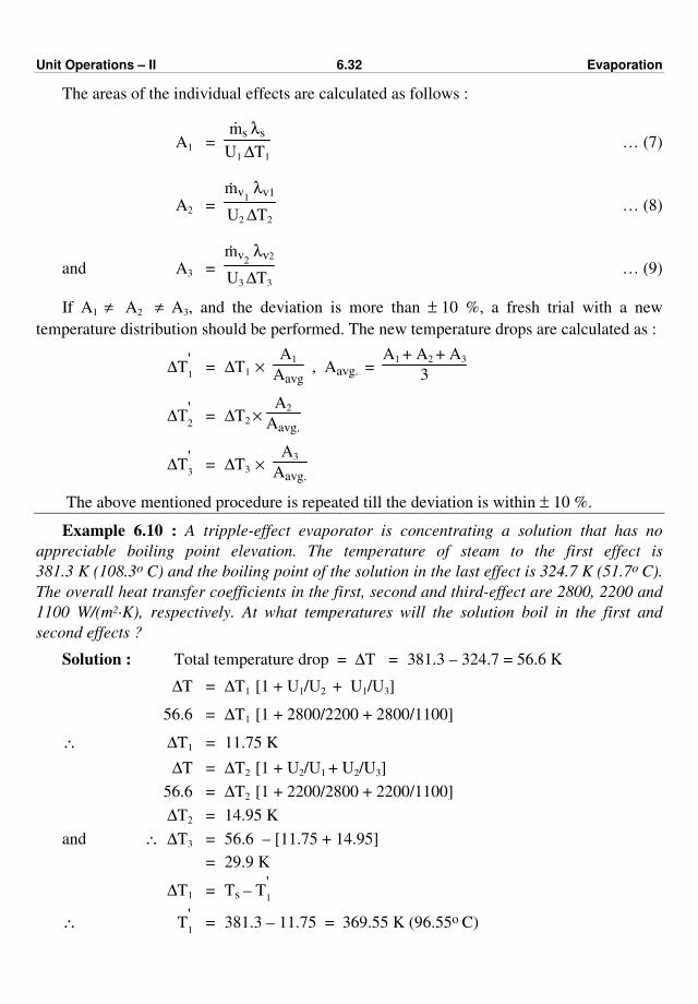
Unit Operations – II 6.32 Evaporation
The areas of the individual effects are calculated as follows :
A1 =
.ms λs
U1 ∆T1
… (7)
A2 =
.mv1
λv1
U2 ∆T2
… (8)
and A3 =
.mv2
λv2
U3 ∆T3
… (9)
If A1 ≠ A2 ≠ A3, and the deviation is more than ± 10 %, a fresh trial with a new
temperature distribution should be performed. The new temperature drops are calculated as :
∆T'1 = ∆T1 ×
A1
Aavg , Aavg. =
A1 + A2 + A3
3
∆T'2 = ∆T2 ×
A2
Aavg.
∆T'3 = ∆T3 ×
A3
Aavg.
The above mentioned procedure is repeated till the deviation is within ± 10 %.
Example 6.10 : A tripple-effect evaporator is concentrating a solution that has no
appreciable boiling point elevation. The temperature of steam to the first effect is
381.3 K (108.3o C) and the boiling point of the solution in the last effect is 324.7 K (51.7o C).
The overall heat transfer coefficients in the first, second and third-effect are 2800, 2200 and
1100 W/(m2·K), respectively. At what temperatures will the solution boil in the first and
second effects ?
Solution : Total temperature drop = ∆T = 381.3 – 324.7 = 56.6 K
∆T = ∆T1 [1 + U1/U2 + U1/U3]
56.6 = ∆T1 [1 + 2800/2200 + 2800/1100]
∴ ∆T1 = 11.75 K
∆T = ∆T2 [1 + U2/U1 + U2/U3]
56.6 = ∆T2 [1 + 2200/2800 + 2200/1100]
∆T2 = 14.95 K
and ∴ ∆T3 = 56.6 – [11.75 + 14.95]
= 29.9 K
∆T1 = Ts – T'1
∴ T'1 = 381.3 – 11.75 = 369.55 K (96.55o C)

Unit Operations – II 6.33 Evaporation
∆T2 = T'1 – T
'2
T'2 = 369.55 – 14.95
= 354.6 K (81.6 oC)
Boiling point in the first effect = 369.55 K (96.55o C) ………… Ans.
Boiling point in the second effect = 354.6 K (81.6o C) ………… Ans.
Example 6.11 : A double-effect evaporator is used to concentrate 10,000 kg/h of
caustic soda solution from 9% to 47% by wt. NaOH. For this purpose, a backward feed
arrangement is used. The feed enters the evaporator at 309 K (36o C). Process steam at
686.616 kPa.g is available and in the second effect a vacuum of 86.66 kPa is maintained.
Design a suitable forced circulation system with equal heating surface in both the effects.
Calculate the steam consumption and evaporation in each effect. Neglect boiling point rise.
The overall heat transfer coefficients in the first and second effects are 2326 and
1744.5 W/(m2·K), respectively. Take a specific heat of 3.77 kJ/(kg·K), for all caustic streams.
Solution : 10,000 kg/h of feed.
ms.ls
Steam
Firsteffect
mv1Hv1
Secondeffect
mv2
Hv2
m1, H'2m'2
H'2Product
47% NaOH
Feed, . Hm
9% NaOHf f
Fig. 6.14
Overall material balance :
⋅
mf = ⋅
m'1 +
⋅mv1 +
⋅mv2
Material balance of solute :
0.09 × 10000 = 0.47 × .
m'1
⋅
m'1 = 1915 kg/h
Steam pressure = 686.616 kPa.g.
= 686.616 + 101.325 = 787.941 kPa
Hence, saturation temperature, Ts = 442.7 K (169.7 oC)
Vacuum in the second effect = 86.660 kPa
Absolute pressure in the second effect = 101.325 – 86.660
= 14.665 kPa

Unit Operations – II 6.34 Evaporation
Corresponding temperature = 326.3 K (53.3 oC)
∴ Overall temperature drop = ∆T = 442.7 – 326.3
= 116.4 K (oC)
Assuming heat loads to be equal in both the effects,
Q1 ~– Q2
U1A1 ∆T1 = U2 A2 ∆T2
For equal heat transfer surface,
U1 ∆T1 = U2 ∆T2
∆T1 = U2
U1 ∆T2 =
2326
1744.5 ∆T2 = 0.75 ∆T2
∆T = ∆T1 + ∆T2 = 0.75 ∆T2 + ∆T2
116.4 = 1.75 ∆T2
∴ ∆T2 = 66.5 K, and ∆T1 = 49.9 K
Since there is no B.P.R.
∆T1 = Ts – Tv1
where Tv1 – temperature in the vapour space of first effect
Tv1 = Ts – ∆T1 = 442.7 – 49.9
Tv1 = 392.8 K (119.8 oC)
Tv2 = Tv1 – ∆T2
= 392.8 – 66.5 = 326.3 K (53.3 oC)
Enthalpies of various streams :
Hf = feed enthalpy
Hf = 3.768 × (309 – 273)
= 135.66 kJ/kg
H'1 = enthalpy of the final product
= 3.768 (392.8 – 273)
= 451.4 kJ/kg
H'2 = enthalpy of the intermediate product
= 3.768 (326.3 – 273) = 200.83 kJ/kg
For steam at 442.7 K (169.7 oC), λs = 2048.7 kJ/kg
For vapour at 392.8 K (119.8 oC)
Hv1 = 2705.22 kJ/kg, λv1 = 2202.8 kJ/kg
For vapour at 326.3 K (53.3 oC)
Hv2 = 2597.61 kJ/kg
λv2 = 2377.8 kJ/kg
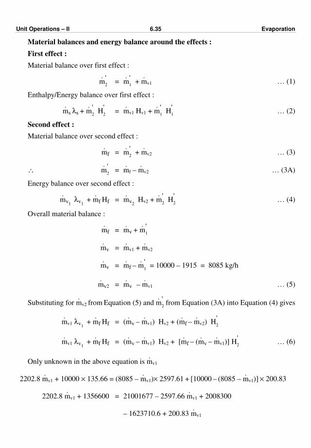
Unit Operations – II 6.35 Evaporation
Material balances and energy balance around the effects :
First effect : ����
Material balance over first effect :
⋅
m'2 =
⋅m
'1 +
⋅mv1 … (1)
Enthalpy/Energy balance over first effect :
⋅
ms λs + ⋅
m'2 H
'2 =
⋅mv1 Hv1 +
⋅m
'1 H
'1 … (2)
Second effect :
Material balance over second effect :
⋅
mf = ⋅
m'2 +
⋅mv2 … (3)
∴ ⋅
m'2 =
⋅mf –
⋅mv2 … (3A)
Energy balance over second effect :
⋅
mv1 λv1
+ ⋅
mf Hf = ⋅
mv2 Hv2 +
⋅m
'2 H
'2 … (4)
Overall material balance :
⋅
mf = ⋅
mv + ⋅
m'1
⋅
mv = ⋅
mv1 + ⋅
mv2
⋅
mv = ⋅
mf – ⋅
m'1 = 10000 – 1915 = 8085 kg/h
⋅
mv2 = ⋅
mv – ⋅
mv1 … (5)
Substituting for ⋅
mv2 from Equation (5) and ⋅
m'2 from Equation (3A) into Equation (4) gives
⋅
mv1 λv1 +
⋅mf Hf = (
⋅mv –
⋅mv1) Hv2 + (
⋅mf –
⋅mv2) H
'2
⋅
mv1 λv1 +
⋅mf Hf = (
⋅mv –
⋅mv1) Hv2 + [
⋅mf – (
⋅mv –
⋅mv1)] H
'2 … (6)
Only unknown in the above equation is ⋅
mv1
2202.8 ⋅
mv1 + 10000 × 135.66 = (8085 – ⋅
mv1)× 2597.61 + [10000 – (8085 – ⋅
mv1)] × 200.83
2202.8 ⋅
mv1 + 1356600 = 21001677 – 2597.66 ⋅
mv1 + 2008300
– 1623710.6 + 200.83 ⋅
mv1
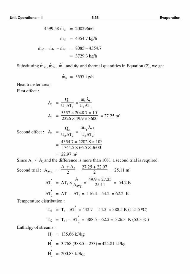
Unit Operations – II 6.36 Evaporation
4599.58 ⋅
mv1 = 20029666
⋅
mv1 = 4354.7 kg/h
⋅
mv2 = ⋅
mv – ⋅
mv1 = 8085 – 4354.7
= 3729.3 kg/h
Substituting ⋅
mv1, ⋅
mv2, ⋅
m'1 and ·mf and thermal quantities in Equation (2), we get
⋅
ms = 5557 kg/h
Heat transfer area :
First effect :
A1 = Q1
U1 ∆T1
=
.ms λs
U1 ∆T1
A1 = 5557 × 2048.7 × 103
2326 × 49.9 × 3600 = 27.25 m2
Second effect : A2 = Q2
U2 ∆T2
=
.mv1
λv1
U2 ∆T2
= 4354.7 × 2202.8 × 103
1744.5 × 66.5 × 3600
= 22.97 m2
Since A1 ≠ A2 and the difference is more than 10%, a second trial is required.
Second trial : Aavg = A1 + A2
2 =
27.25 + 22.97
2 = 25.11 m2
∆T'1 = ∆T1 ×
A1
Aavg =
49.9 × 27.25
25.11 = 54.2 K
∆T'2 = ∆T – ∆T1 = 116.4 – 54.2 = 62.2 K
Temperature distribution :
Tv1 = Ts – ∆T'1 = 442.7 – 54.2 = 388.5 K (115.5 oC)
Tv2 = Tv1 – ∆T'2 = 388.5 – 62.2 = 326.3 K (53.3 oC)
Enthalpy of streams :
Hf = 135.66 kJ/kg
H'1 = 3.768 (388.5 – 273) = 424.81 kJ/kg
H'2 = 200.83 kJ/kg
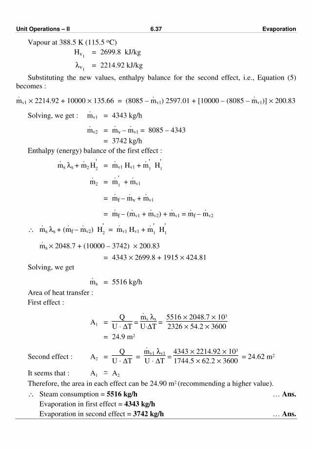
Unit Operations – II 6.37 Evaporation
Vapour at 388.5 K (115.5 oC)
Hv1 = 2699.8 kJ/kg
λv1 = 2214.92 kJ/kg
Substituting the new values, enthalpy balance for the second effect, i.e., Equation (5)
becomes :
⋅mv1 × 2214.92 + 10000 × 135.66 = (8085 –
⋅mv1) 2597.01 + [10000 – (8085 –
⋅mv1)] × 200.83
Solving, we get : ⋅
mv1 = 4343 kg/h
⋅
mv2 = ⋅
mv – ⋅
mv1 = 8085 – 4343
= 3742 kg/h
Enthalpy (energy) balance of the first effect :
⋅
ms λs + ⋅
m2 H'2 =
⋅mv1 Hv1 +
⋅m
'1 H
'1
⋅
m2 = ⋅
m'1 +
⋅mv1
= ⋅
mf – ⋅
mv + ⋅
mv1
= ⋅
mf – (⋅
mv1 + ⋅
mv2) + ⋅
mv1 = ⋅
mf – ⋅
mv2
∴ ⋅
ms λs + (⋅
mf – ⋅
mv2) H'2 =
⋅mv1 Hv1 +
⋅m
'1 H
'1
⋅
ms × 2048.7 + (10000 – 3742) × 200.83
= 4343 × 2699.8 + 1915 × 424.81
Solving, we get
⋅
ms = 5516 kg/h
Area of heat transfer :
First effect :
A1 = Q
U ⋅ ∆T =
⋅ms λs
U⋅∆T =
5516 × 2048.7 × 103
2326 × 54.2 × 3600
= 24.9 m2
Second effect : A2 = Q
U ⋅ ∆T =
⋅mv1 λv1
U ⋅ ∆T =
4343 × 2214.92 × 103
1744.5 × 62.2 × 3600 = 24.62 m2
It seems that : A1 ~– A2
Therefore, the area in each effect can be 24.90 m2 (recommending a higher value).
∴ Steam consumption = 5516 kg/h … Ans.
Evaporation in first effect = 4343 kg/h
Evaporation in second effect = 3742 kg/h … Ans.
Unit Operations – II 6.38 Evaporation
EXERCISES
1. Fill in the blanks :
(a) The weak liquor to be fed to the evaporator is composed of a non-volatile
......... and a ....... solvent. Ans. solute, volatile
(b) In most of the evaporation operation ........ are condensed and discarded.
Ans. water vapour
(c) .......... is carried out by supplying heat to a solution to vaporise the solvent.
Ans. Evaporation
(d) In case of evaporation generally the ........... is the valuable product.
Ans. concentrated solution / thick liquor
(e) In the .......... feed system, vapour and liquor flow in counter current fashion.
Ans. backward
(f) Economy of a single-effect evaporator is always less than ........ Ans. one
(g) Economy of a multiple effect evaporator system is always .... than one.
Ans. more or greater
(h) In ............ evaporator, the velocity of liquid entering the tube is of the order of
2 to 6 m/s. Ans. forced circulation
(i) ......... tube vertical evaporator is commonly used for handling solutions that
tend to foam. Ans. Long
(j) In case of Calendria type evaporator the solution to be evaporated is ......... the
tubes and steam flows ........... the tubes in the steam chest. Ans. inside, outside
2. Define the following terms :
(i) evaporation (ii) boiling point elevation (iii) capacity of an evaporator and
(iv) economy of an evaporator.
3. Why the economy of single effect evaporator is less than one ?
4. State the method of increasing the economy of an evaporator.
5. What do you mean by multiple-effect evaporation system ?
6. What do you mean by double-effect evaporator ?
7. State the method of feeding multiple-effect evaporation system.
8. Compare forward feed arrangement with backward feed arrangement in case of a
multiple effect evaporation system.
9. State the advantages of forced circulation evaporators and its application.
10. Explain the construction with a neat sketch of standard vertical tube evaporator.
11. Draw neat diagrams of forward feed arrangement and backward feed arrangement
for feeding multiple effect evaporation system.
12. State some examples of evaporation operation.
13. Draw a neat sketch of long tube evaporator and explain briefly its construction and
working.
14. Explain in brief forced circulation evaporator with an external horizontal heating
surface with reference to its construction and working.
15. Explain in brief vapour recompression with a neat sketch.
ppp
(7.1)
CHAPTER SEVEN
DIFFUSION
In a mixture consisting of two or more components, if the concentrations of the
components vary from point to point, then there is a natural tendency for each component to
migrate/move from regions of high concentration to those of low concentration. The process
of transfer of mass as a result of the concentration difference of a component in a mixture or
two phases in contact is called mass transfer.
The operations carried out for separating the components of a mixture, involving the
transfer of material from one homogeneous phase to another, utilising the difference in
vapour pressure, solubility or diffusivity and in which the driving force for transfer is a
concentration difference are called as mass transfer operations.
In case of evaporation of water from a pool of water into a stream of air flowing over the
water surface, molecules of water vapour diffuse through those of the air at the surface into
the main portion of air stream, as a result of which they are carried away with the air flowing.
In this case, mass transfer is a result of a concentration difference or gradient, the diffusing
substance (water) moving from a region of high concentration to a region of low
concentration. Hence, the driving force for mass transfer is a concentration difference just as
a temperature difference in heat transfer.
Fractional distillation (one of the methods of separation) depends on the difference in
vapour pressures of different components at the same temperature (volatility), while gas
absorption depends on the difference in solubility of gases in a selective solvent. Liquid-
liquid extraction and leaching depend on the difference in solubility in a liquid solvent.
Mass transfer operations include separation techniques such as distillation, gas
absorption, liquid extraction, drying, crystallisation, etc.
In mass transfer operations, mass transfer may occur :
(a) In one direction, e.g., gas absorption.
(b) In opposite directions (i.e., in both directions), e.g., distillation.
(c) With simultaneous heat transfer, e.g., drying and crystallisation.
(d) With a simultaneous chemical reaction, e.g., gas absorption accompanied by a
chemical reaction (absorption of CO2 in an aqueous solution of KOH)
(e) With the exchange of one or more components.
(f) Isothermally (i.e., at constant T) and non-isothermally.
The phenomena those must exist in mass transfer operations are :
(a) At least two phases must come in contact with each other.
(b) Materials must flow from one phase to the other.
(c) A part of the total flow of material must occur by molecular diffusion.
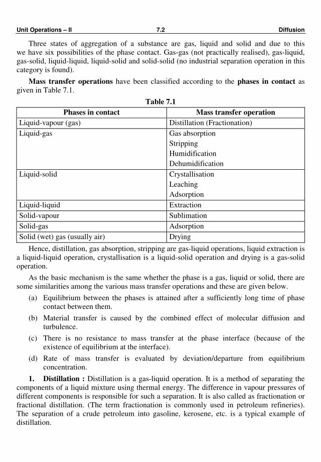
Unit Operations – II 7.2 Diffusion
Three states of aggregation of a substance are gas, liquid and solid and due to this
we have six possibilities of the phase contact. Gas-gas (not practically realised), gas-liquid,
gas-solid, liquid-liquid, liquid-solid and solid-solid (no industrial separation operation in this
category is found).
Mass transfer operations have been classified according to the phases in contact as
given in Table 7.1.
Table 7.1
Phases in contact Mass transfer operation
Liquid-vapour (gas) Distillation (Fractionation)
Liquid-gas
Gas absorption
Stripping
Humidification
Dehumidification
Liquid-solid
Crystallisation
Leaching
Adsorption
Liquid-liquid Extraction
Solid-vapour Sublimation
Solid-gas Adsorption
Solid (wet) gas (usually air) Drying
Hence, distillation, gas absorption, stripping are gas-liquid operations, liquid extraction is
a liquid-liquid operation, crystallisation is a liquid-solid operation and drying is a gas-solid
operation.
As the basic mechanism is the same whether the phase is a gas, liquid or solid, there are
some similarities among the various mass transfer operations and these are given below.
(a) Equilibrium between the phases is attained after a sufficiently long time of phase
contact between them.
(b) Material transfer is caused by the combined effect of molecular diffusion and
turbulence.
(c) There is no resistance to mass transfer at the phase interface (because of the
existence of equilibrium at the interface).
(d) Rate of mass transfer is evaluated by deviation/departure from equilibrium
concentration.
1. Distillation : Distillation is a gas-liquid operation. It is a method of separating the
components of a liquid mixture using thermal energy. The difference in vapour pressures of
different components is responsible for such a separation. It is also called as fractionation or
fractional distillation. (The term fractionation is commonly used in petroleum refineries).
The separation of a crude petroleum into gasoline, kerosene, etc. is a typical example of
distillation.
Unit Operations – II 7.3 Diffusion
Consider a binary liquid mixture. For this, we have : C = 2, P = 2.
∴ F = 2 (phase rule : F = C – P + 2). In this case there are four variables; temperature,
pressure, composition of A in the liquid and vapour phases. If the pressure is fixed, then
according to the phase rule only one variable, e.g., the liquid phase concentration can be
varied and the temperature and vapour phase concentration follow and thus the system is
defined completely. Here the equilibrium data are presented in temperature-composition
diagrams at constant pressure or by plotting vapour phase composition against liquid phase
composition. Such a plot is called the equilibrium curve.
2. Gas absorption : Gas absorption is a gas-liquid operation. It is a method of
separating one or more constituents of a gas mixture by contacting it with a suitable liquid
solvent. The necessary condition is the difference in solubility of the constituents in a given
solvent. The washing of ammonia from a ammonia-air mixture by means of water is a typical
example of gas absorption.
Consider that a gas mixture contains two components and one component is transferred.
Thus, we have C = 3, P = 2 and ∴ F = 3. There are four variables : temperature pressure,
and the concentration of A in liquid and gas phases. If the temperature and pressure are fixed,
one concentration may be chosen as the remaining independent variable that may be varied
and the other concentration follows. A plot of equilibrium concentration in the gas phase v/s
concentration in the liquid phase gives an equilibrium relationship between the phases.
3. Liquid extraction : Liquid extraction is a liquid-liquid operation. It is a method of
separating the constituents of a liquid mixture by treating it with a suitable solvent that
preferentially dissolves one or more of the constituents of the mixture. It is also called as
solvent extraction. It is used as a separation technique only when distillation is ineffective
and difficult. The separation of penicillin from fermentation mixtures is a typical example of
application of liquid extraction.
4. Crystallisation : It is a liquid-solid operation and used to obtain materials in the
form of attractive and uniform crystals of good purity. Crystallisation is the formation of
solid particles within a homogeneous liquid phase.
5. Drying : Drying is a gas-solid operation. In general, it is the removal of moisture of
a substance.
In case of drying, there are two phases and three components. C = 3, P = 2, ∴ F = 3.
The variables are : temperature, pressure, the concentration of water in the solid and the
gas phases. If the temperature and pressure are fixed, one concentration may be taken as the
remaining independent variable and the other concentration follows. These two
concentrations can be plotted as the equilibrium curve.
DIFFUSION It is the movement of an individual component through a mixture from a region of higher
concentration to a region of lower concentration at fixed temperature and pressure with or
without the help of an external force.
A mixture which is non-uniform initially will be ultimately brought to uniformity
(a mixture is everywhere uniform in the concentration of its constituents) by diffusion since
the concentration gradient which acts as a driving force for diffusion tends to move the
component in such a direction as to equalise concentrations and destroy the gradient. If we
maintain the concentration gradient by constantly supplying the diffusing component to the
Unit Operations – II 7.4 Diffusion
high concentration end and removing it at the low concentration end, then the flow of
diffusing component is continuous. This movement is utilised in mass transfer operations.
When diffusion results from the random movement/motion of the molecules, it is called
molecular diffusion. As the molecular diffusion requires actual migration of molecules, the
rate of mass transfer is higher in gases than liquids and very slow in solids. When the
movement of the molecules occurs with the help of an external force (e.g., mechanical
stirring and convective movement of the fluid), then it is called eddy or turbulent diffusion.
The molecular diffusion is a slow process, whereas the eddy diffusion is a fast process. The
molecular diffusion is the mechanism of a stationary fluid, i.e., a fluid at rest and fluids in
laminar flow. In case of fluids in turbulent flow, the mechanism of mass transfer is by eddy
diffusion. The transfer of material in the presence of a concentration gradient is classified as
molecular transfer and eddy transfer. Molecular transfer of mass occurs in stationary fluids or
fluids in laminar flow whereas eddy transfer occurs in fluids under turbulent conditions.
Role of diffusion in mass transfer : Diffusion may occur in one phase or in both phases in all the mass transfer operations.
In case of distillation, the more volatile component diffuses through the liquid phase to the
interface between the phases (liquid and vapour phases) and away from the interface into the
vapour phase. The less volatile component diffuses in the opposite direction and passes from
the vapour phase to the liquid phase. In case of gas absorption, the solute gas diffuses
through the gas phase to the interface and then through the liquid phase (liquid solvent
phase) from the interface between the phases. In case of crystallisation, the solid solute
diffuses through the mother liquor (liquid phase) to the crystals and deposit on the solid
surfaces. In case of drying operation, liquid water (moisture) diffuses through the solid
towards the surface of the solid, evaporates and diffuses as a vapour into the gas phase
(drying medium). In case of liquid-liquid extraction, the liquid solute diffuses through the
raffinate phase and then into the extract phase (solvent phase) from the interface between
the phases.
Molecular Diffusion :
Concentrations, velocities and fluxes :
Let us consider two chemical species A and B are placed in two compartments that are
separated by a impermeable partition. Now, assume that the partition is suddenly removed so
that the species A will diffuse into B and the species B will diffuse in A and this will
continue at a constantly decreasing rate until the mixture becomes everywhere uniform in the
concentration of its constituents, i.e., of A and B. The process is one of molecular diffusion
in which the species are diffused in one another as a result of the random motion of
molecules. The rate of diffusion is governed by Fick's law and before dealing with this law,
we will define the above mentioned terms based on the combination of such species. We
make it clear here that by the word solution we mean a mixture of species of the same phase
– gas in gas, liquid in liquid, etc., i.e., one phase - a gaseous, a liquid or a solid mixture.
Concentration :
There are various ways to express the concentration of the various species in a
multicomponent system/mixture. We limit our discussion to mass concentration, molar/
concentration, mass fraction and mole fraction.
Unit Operations – II 7.5 Diffusion
Mass concentration : The mass concentration of a species A in a solution is the mass of
species A per unit volume of the solution (mixture). It is equivalent to the density of A and
denoted by the symbol ρA.
For a binary mixture/solution of A and B,
ρA + ρB = ρ … (7.1)
where ρ is the mass density of the solution.
Molar concentration : The molar concentration of a species A in a solution is the
number of moles of species A per unit volume of the solution.
CA = ρA
MA … (7.2)
where MA is the molecular weight of component A. The unit of molar concentration in the
SI system is kmol/m3.
Hence, for a binary mixture of A and B, the total molar concentration of the mixture is
given by
C = CA + CB … (7.3)
Mass fraction : The mass fraction x'A of a species A in a solution may be defined as the
ratio of the mass concentration of species A to the mass density of the solution.
x'A =
ρA
ρ … (7.4)
Mole fraction : The mole fraction (xA) of a species A in a solution may be defined as the
ratio of the molar concentration of A to the molar concentration of the solution.
xA = CA
C … (7.5)
For a binary system of A and B, we have
x'A + x
'B = 1
and xA + xB = 1
In the gas phase, concentrations are usually expressed in terms of partial pressures.
For an ideal gas A, pAV = nART
CA = nA
V =
pA
RT … (7.6)
where pA is the partial pressure of species A in the mixture, nA is the number of moles of A in
the mixture, V is the molar volume of the mixture, T is the temperature (absolute), and R is
the univeral gas constant.
xA in terms of pA is given as :
xA = CA
C =
pA/RT
P/RT =
pA
P … (7.7)
where P is the total pressure exerted by the gas mixture.
Also, we have C = CA + CB = pA
RT +
pB
RT =
P
RT … (7.8)

Unit Operations – II 7.6 Diffusion
Velocities :
In a diffusing mixture, various chemical species are moving at different velocities as they
may have different mobilities. The bulk velocity of the mixture would be some sort of an
average velocity. Let ui be the velocity of the ith species with respect to the stationary
coordinate system. Then, for a mixture of n species, the local mass average velocity u is
defined by
u =
n
∑i = 1
ρi ui
n
∑i = 1
ρi
… (7.9)
ρu is the local rate at which mass passes through a unit cross-section when it is placed
perpendicular to u.
For a binary system of A and B components, we can write
u = ρA uA + ρB uB
ρ … (7.10)
The local molar average velocity of the mixture, U, is defined by
U =
n
∑i = 1
Ci ui
n
∑i = 1
Ci
… (7.11)
Cu is the local rate at which moles pass through a unit cross-section which is placed
perpendicular to U.
For a binary system of A and B, we can write
U = CAuA + CB uB
C … (7.12)
Let us define two diffusion velocities relative to/with respect to the two bulk velocities
(mass and molar average velocities of the mixture).
The mass diffusion velocity of a species is the velocity of that species relative to the local
mass average velocity of the mixture.
Mass diffusion velocity of species i w.r.t. u = ui – u
Mass diffusion velocity of species A w.r.t. u = uA – u.
The molar diffusion velocity of a species is the velocity of species with respect to/relative
to the local molar average velocity of the mixture.
Molar diffusion velocity of species i w.r.t. U = ui – U … (7.13)
Molar diffusion velocity of species A w.r.t. U = uA – U … (7.14)
Mass flow rate : It is the quantity of material flow in mass units per unit time (e.g., kg/s)
Molar flow rate : It is the quantity of material flow in molar units per unit time
(e.g., kmol/s).

Unit Operations – II 7.7 Diffusion
Flux : The mass transfer flux of a given species (vector quantity) is defined as the
amount of that species, in either mass or, molar units, that crosses a unit area per unit time.
We will define four types of fluxes, two with reference to fixed coordinates in space and two
with respect to local mass average velocity and local molar average velocity (w.r.t.
coordinates moving with mass average velocity and molar average velocity).
Mass flux : The mass flux of a species i is defined as the mass of species i that passes
through a unit area per unit time.
The mass flux relative to stationary/fixed coordinates is given by
ni = ρi ui … (7.15)
The mass flux relative to the mass average velocity u is given by
ji = ρi (ui – u) … (7.16)
Molar flux : It is defined as the moles of species i that passes through a unit area per unit
time.
The molar flux relative to stationary coordinates is given by
Ni = Ci ui … (7.17)
The molar flux relative to the molar average velocity U is given by
Ji = Ci (ui – U) … (7.18)
It is true that any one of the above mentioned notation used for the flux is adequate for all
diffusion problems, but each has certain advantages. In process calculations, it is usually
desirable to refer to a coordinate system fixed in an equipment so the flux Ni is used in
engineering. The fluxes ji and Ji are the usual measures of rates of diffusion and are useful in
formulating the equations of change for multicomponent systems.
For a binary system of A and B :
The mass fluxes of A and B relative to stationary coordinates are :
nA = ρA uA … (7.19)
nB = ρB uB … (7.20)
The mass fluxes of A and B relative to mass average velocity are :
jA = ρA (uA – u) … (7.21)
jB = ρB (uB – u) … (7.22)
The molar fluxes of A and B with respect to stationary coordinates are :
NA = CA uA … (7.23)
NB = CB uB … (7.24)
The molar fluxes of A and B relative to molar average velocity U are :
JA = CA (uA – U) … (7.25)
JB = CB (uB – U) … (7.26)

Unit Operations – II 7.8 Diffusion
JA and JB are the diffusion flux of components A and B. The various fluxes can be
interrelated as,
nA = ρA uA
= ρA (u + uA – u)
= ρA u + ρA (uA – u)
= ρA u + ji … (7.27)
We have, x'A =
ρA
ρ ∴ ρA = x
'A ρ
nA = x'A (ρu) + ji
Since, ∑ ni = ∑ ρi ui = ρv
∴ nA = x'A ∑ ni + ji … (7.28)
Similarly, NA = CA uA
= CA (U + uA – U)
= CA U + CA (uA – U)
NA = CA U + JA … (7.29)
NA = xA (CU) + JA
∑ Ni = ∑ Ci ui = CU
NA = xA (∑ Ni) + JA … (7.30)
Fick's law of diffusion :
A relation between the flux of the diffusing substance and the concentration gradient
responsible for molecular diffusion-mass transfer was first proposed by FICK in 1855 and is
therefore referred to as Fick's first law of diffusion.
The flux of a diffusing component A (diffusion flux of A) in z direction in a binary mixture
of A and B is proportional to the concentration gradient.
Therefore, the Fick's law of diffusion for species/component A in a binary mixture of A
and B for steady state diffusion in z direction can be expressed as
JA = – DAB · dCA
dz … (7.31)
where JA is the molar flux of A in the z direction relative to the molar average velocity [moles
per unit area per unit time, kmol/(m2.s)].
CA is the molar concentration of A [moles of A per unit volume, kmol/m3]
dCA
dz is the concentration gradient in the z-direction.
DAB is a proportionality constant, known as the molecular diffusivity or diffusion
coefficient for component A diffusing through B, m2/s and z is the distance in the direction of
diffusion, m.
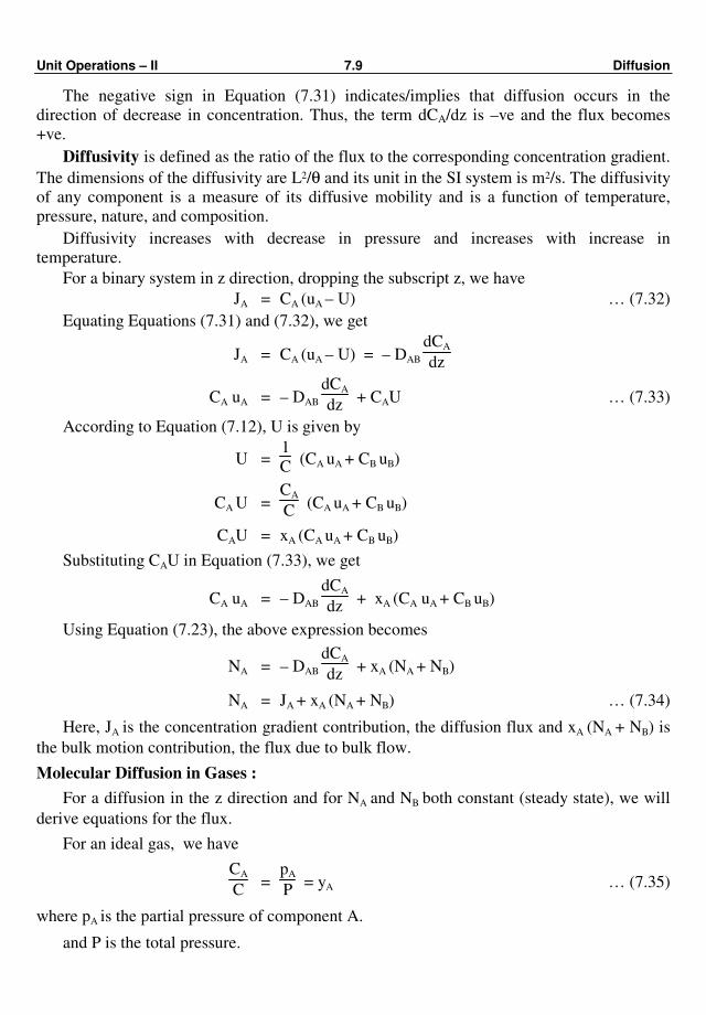
Unit Operations – II 7.9 Diffusion
The negative sign in Equation (7.31) indicates/implies that diffusion occurs in the
direction of decrease in concentration. Thus, the term dCA/dz is –ve and the flux becomes
+ve.
Diffusivity is defined as the ratio of the flux to the corresponding concentration gradient.
The dimensions of the diffusivity are L2/θ and its unit in the SI system is m2/s. The diffusivity
of any component is a measure of its diffusive mobility and is a function of temperature,
pressure, nature, and composition.
Diffusivity increases with decrease in pressure and increases with increase in
temperature.
For a binary system in z direction, dropping the subscript z, we have
JA = CA (uA – U) … (7.32)
Equating Equations (7.31) and (7.32), we get
JA = CA (uA – U) = – DAB
dCA
dz
CA uA = – DAB
dCA
dz + CAU … (7.33)
According to Equation (7.12), U is given by
U = 1
C (CA uA + CB uB)
CA U = CA
C (CA uA + CB uB)
CAU = xA (CA uA + CB uB)
Substituting CAU in Equation (7.33), we get
CA uA = – DAB
dCA
dz + xA (CA uA + CB uB)
Using Equation (7.23), the above expression becomes
NA = – DAB
dCA
dz + xA (NA + NB)
NA = JA + xA (NA + NB) … (7.34)
Here, JA is the concentration gradient contribution, the diffusion flux and xA (NA + NB) is
the bulk motion contribution, the flux due to bulk flow.
Molecular Diffusion in Gases :
For a diffusion in the z direction and for NA and NB both constant (steady state), we will
derive equations for the flux.
For an ideal gas, we have
CA
C =
pA
P = yA … (7.35)
where pA is the partial pressure of component A.
and P is the total pressure.
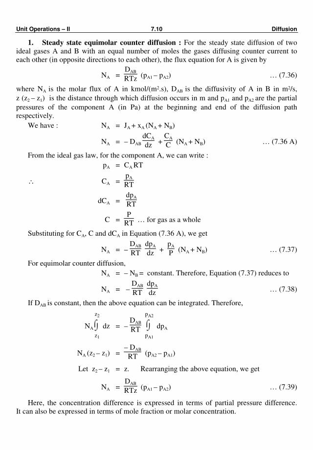
Unit Operations – II 7.10 Diffusion
1. Steady state equimolar counter diffusion : For the steady state diffusion of two
ideal gases A and B with an equal number of moles the gases diffusing counter current to
each other (in opposite directions to each other), the flux equation for A is given by
NA = DAB
RTz (pA1 – pA2) … (7.36)
where NA is the molar flux of A in kmol/(m2.s), DAB is the diffusivity of A in B in m2/s,
z (z2 – z1) is the distance through which diffusion occurs in m and pA1 and pA2 are the partial
pressures of the component A (in Pa) at the beginning and end of the diffusion path
respectively.
We have : NA = JA + xA (NA + NB)
NA = – DAB
dCA
dz +
CA
C (NA + NB) … (7.36 A)
From the ideal gas law, for the component A, we can write :
pA = CA RT
∴ CA = pA
RT
dCA = dpA
RT
C = P
RT … for gas as a whole
Substituting for CA, C and dCA in Equation (7.36 A), we get
NA = – DAB
RT
dpA
dz +
pA
P (NA + NB) … (7.37)
For equimolar counter diffusion,
NA = – NB = constant. Therefore, Equation (7.37) reduces to
NA = – DAB
RT
dpA
dz … (7.38)
If DAB is constant, then the above equation can be integrated. Therefore,
NA ⌡⌠
z1
z2
dz = – DAB
RT ⌡⌠
pA1
pA2
dpA
NA (z2 – z1) = – DAB
RT (pA2 – pA1)
Let z2 – z1 = z. Rearranging the above equation, we get
NA = DAB
RTz (pA1 – pA2) … (7.39)
Here, the concentration difference is expressed in terms of partial pressure difference.
It can also be expressed in terms of mole fraction or molar concentration.
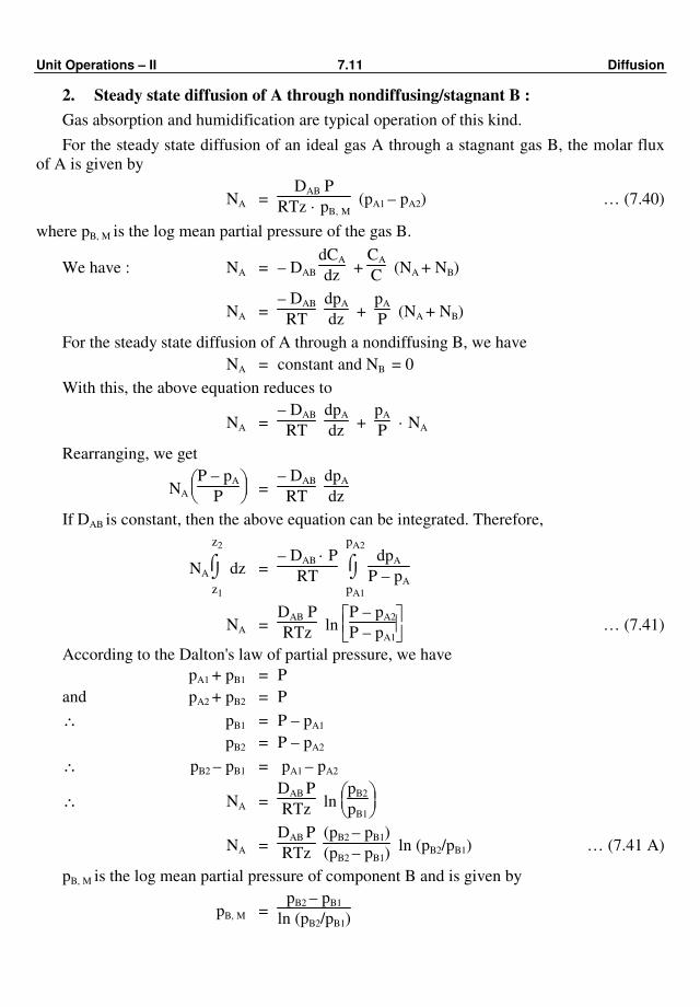
Unit Operations – II 7.11 Diffusion
2. Steady state diffusion of A through nondiffusing/stagnant B :
Gas absorption and humidification are typical operation of this kind.
For the steady state diffusion of an ideal gas A through a stagnant gas B, the molar flux
of A is given by
NA = DAB P
RTz · pB‚ M (pA1 – pA2) … (7.40)
where pB, M is the log mean partial pressure of the gas B.
We have : NA = – DAB
dCA
dz +
CA
C (NA + NB)
NA = – DAB
RT
dpA
dz +
pA
P (NA + NB)
For the steady state diffusion of A through a nondiffusing B, we have
NA = constant and NB = 0
With this, the above equation reduces to
NA = – DAB
RT
dpA
dz +
pA
P · NA
Rearranging, we get
NA
P – pA
P =
– DAB
RT
dpA
dz
If DAB is constant, then the above equation can be integrated. Therefore,
NA ⌡⌠
z1
z2
dz = – DAB · P
RT ⌡⌠
pA1
pA2
dpA
P – pA
NA = DAB P
RTz ln
P – pA2
P – pA1 … (7.41)
According to the Dalton's law of partial pressure, we have
pA1 + pB1 = P
and pA2 + pB2 = P
∴ pB1 = P – pA1
pB2 = P – pA2
∴ pB2 – pB1 = pA1 – pA2
∴ NA = DAB P
RTz ln
pB2
pB1
NA = DAB P
RTz
(pB2 – pB1)
(pB2 – pB1) ln (pB2/pB1) … (7.41 A)
pB, M is the log mean partial pressure of component B and is given by
pB, M = pB2 – pB1
ln (pB2/pB1)
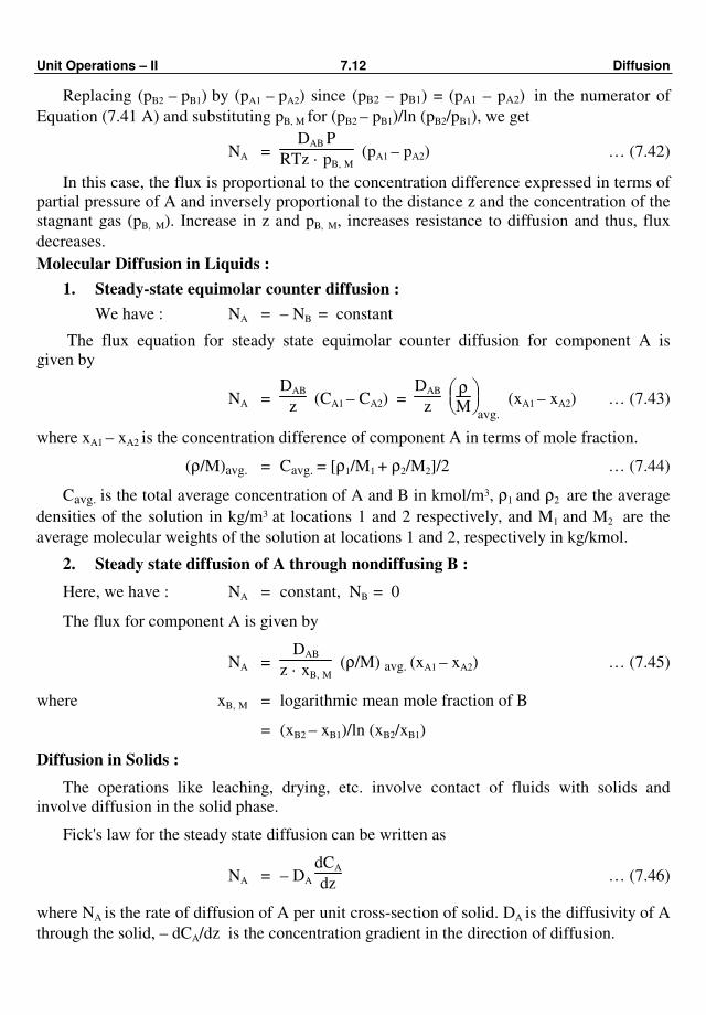
Unit Operations – II 7.12 Diffusion
Replacing (pB2 – pB1) by (pA1 – pA2) since (pB2 – pB1) = (pA1 – pA2) in the numerator of
Equation (7.41 A) and substituting pB, M for (pB2 – pB1)/ln (pB2/pB1), we get
NA = DAB P
RTz · pB‚ M (pA1 – pA2) … (7.42)
In this case, the flux is proportional to the concentration difference expressed in terms of
partial pressure of A and inversely proportional to the distance z and the concentration of the
stagnant gas (pB, M). Increase in z and pB, M, increases resistance to diffusion and thus, flux
decreases.
Molecular Diffusion in Liquids :
1. Steady-state equimolar counter diffusion :
We have : NA = – NB = constant
The flux equation for steady state equimolar counter diffusion for component A is
given by
NA = DAB
z (CA1 – CA2) =
DAB
z
ρ
Mavg.
(xA1 – xA2) … (7.43)
where xA1 – xA2 is the concentration difference of component A in terms of mole fraction.
(ρ/M)avg. = Cavg. = [ρ1/M1 + ρ2/M2]/2 … (7.44)
Cavg. is the total average concentration of A and B in kmol/m3, ρ1 and ρ2 are the average
densities of the solution in kg/m3 at locations 1 and 2 respectively, and M1 and M2 are the
average molecular weights of the solution at locations 1 and 2, respectively in kg/kmol.
2. Steady state diffusion of A through nondiffusing B :
Here, we have : NA = constant, NB = 0
The flux for component A is given by
NA = DAB
z · xB‚ M (ρ/M) avg. (xA1 – xA2) … (7.45)
where xB‚ M = logarithmic mean mole fraction of B
= (xB2 – xB1)/ln (xB2/xB1)
Diffusion in Solids :
The operations like leaching, drying, etc. involve contact of fluids with solids and
involve diffusion in the solid phase.
Fick's law for the steady state diffusion can be written as
NA = – DA
dCA
dz … (7.46)
where NA is the rate of diffusion of A per unit cross-section of solid. DA is the diffusivity of A
through the solid, – dCA/dz is the concentration gradient in the direction of diffusion.
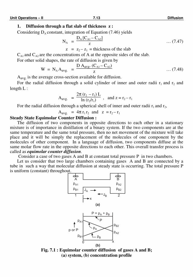
Unit Operations – II 7.13 Diffusion
1. Diffusion through a flat slab of thickness z :
Considering DA constant, integration of Equation (7.46) yields
NA = DA [CA1 – CA2]
z … (7.47)
z = z2 – z1 = thickness of the slab
CA1 and CA2 are the concentrations of A at the opposite sides of the slab.
For other solid shapes, the rate of diffusion is given by
W = NA Aavg. = D Aavg. (CA1 – CA2)
z … (7.48)
Aavg. is the average cross-section available for diffusion.
For the radial diffusion through a solid cylinder of inner and outer radii r1 and r2 and
length L :
Aavg. = 2π (r2 – r1) L
ln (r2/r1) , and z = r2 – r1
For the radial diffusion through a spherical shell of inner and outer radii r1 and r2,
Aavg. = 4π r1 r2 and z = r2 – r1
Steady State Equimolar Counter Diffusion : The diffusion of two components in opposite directions to each other in a stationary mixture is of importance in distillation of a binary system. If the two components are at the same temperature and the same total pressure, then no net movement of the mixture will take place and it will be simply the replacement of the molecules of one component by the molecules of other component. In a language of diffusion, two components diffuse at the same molar flow rate in the opposite directions to each other. This overall transfer process is called as equimolar counter diffusion. Consider a case of two gases A and B at constant total pressure P in two chambers. Let us consider that two large chambers containing gases A and B are connected by a tube in such a way that molecular diffusion at steady state is occurring. The total pressure P is uniform (constant) throughout.
A B
pA1
pB1
pA2
pB2JA
JBx
1 2
P = p + pBA
P
p or PpA
pB
pB2
pA1
pA2
0 x
pB1
(a)
(b) Fig. 7.1 : Equimolar counter diffusion of gases A and B;
(a) system, (b) concentration profile
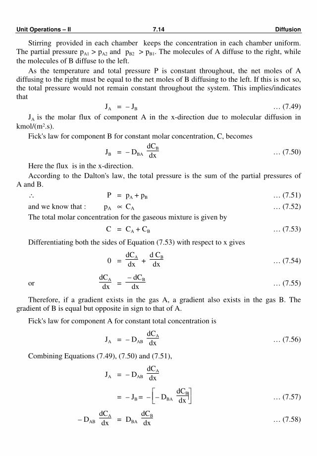
Unit Operations – II 7.14 Diffusion
Stirring provided in each chamber keeps the concentration in each chamber uniform.
The partial pressure pA1 > pA2 and pB2 > pB1. The molecules of A diffuse to the right, while
the molecules of B diffuse to the left.
As the temperature and total pressure P is constant throughout, the net moles of A
diffusing to the right must be equal to the net moles of B diffusing to the left. If this is not so,
the total pressure would not remain constant throughout the system. This implies/indicates
that
JA = – JB … (7.49)
JA is the molar flux of component A in the x-direction due to molecular diffusion in
kmol/(m2.s).
Fick's law for component B for constant molar concentration, C, becomes
JB = – DBA dCB
dx … (7.50)
Here the flux is in the x-direction.
According to the Dalton's law, the total pressure is the sum of the partial pressures of
A and B.
∴ P = pA + pB … (7.51)
and we know that : pA ∝ CA … (7.52)
The total molar concentration for the gaseous mixture is given by
C = CA + CB … (7.53)
Differentiating both the sides of Equation (7.53) with respect to x gives
0 = dCA
dx +
d CB
dx … (7.54)
or dCA
dx =
– dCB
dx … (7.55)
Therefore, if a gradient exists in the gas A, a gradient also exists in the gas B. The
gradient of B is equal but opposite in sign to that of A.
Fick's law for component A for constant total concentration is
JA = – DAB dCA
dx … (7.56)
Combining Equations (7.49), (7.50) and (7.51),
JA = – DAB dCA
dx
= – JB = –
– DBA dCB
dx … (7.57)
– DAB dCA
dx = DBA
dCB
dx … (7.58)
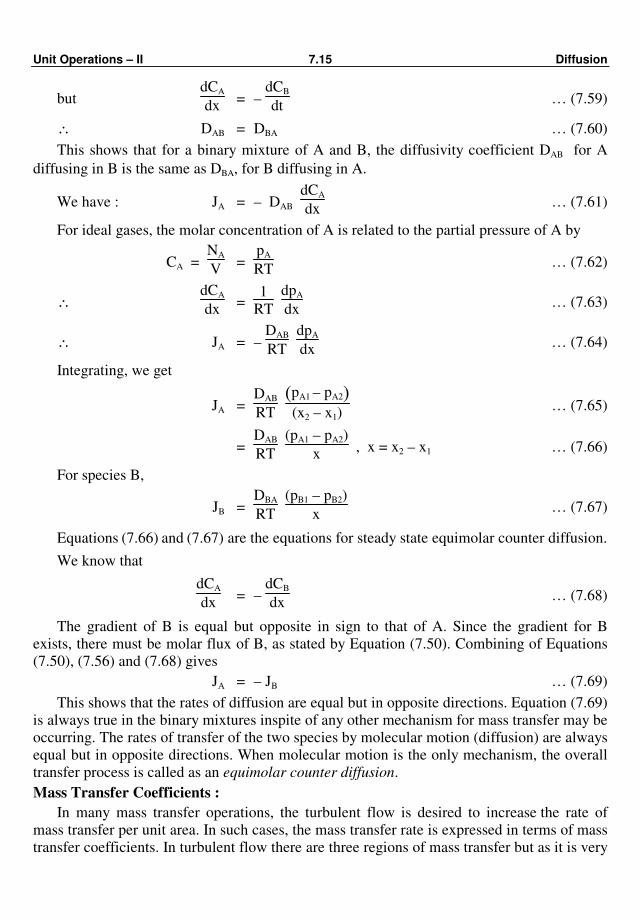
Unit Operations – II 7.15 Diffusion
but dCA
dx = –
dCB
dt … (7.59)
∴ DAB = DBA … (7.60)
This shows that for a binary mixture of A and B, the diffusivity coefficient DAB for A
diffusing in B is the same as DBA, for B diffusing in A.
We have : JA = – DAB dCA
dx … (7.61)
For ideal gases, the molar concentration of A is related to the partial pressure of A by
CA = NA
V =
pA
RT … (7.62)
∴ dCA
dx =
1
RT
dpA
dx … (7.63)
∴ JA = – DAB
RT
dpA
dx … (7.64)
Integrating, we get
JA = DAB
RT ( )pA1 – pA2
(x2 – x1) … (7.65)
= DAB
RT
(pA1 – pA2)
x , x = x2 – x1 … (7.66)
For species B,
JB = DBA
RT
(pB1 – pB2)
x … (7.67)
Equations (7.66) and (7.67) are the equations for steady state equimolar counter diffusion.
We know that
dCA
dx = –
dCB
dx … (7.68)
The gradient of B is equal but opposite in sign to that of A. Since the gradient for B
exists, there must be molar flux of B, as stated by Equation (7.50). Combining of Equations
(7.50), (7.56) and (7.68) gives
JA = – JB … (7.69)
This shows that the rates of diffusion are equal but in opposite directions. Equation (7.69)
is always true in the binary mixtures inspite of any other mechanism for mass transfer may be
occurring. The rates of transfer of the two species by molecular motion (diffusion) are always
equal but in opposite directions. When molecular motion is the only mechanism, the overall
transfer process is called as an equimolar counter diffusion.
Mass Transfer Coefficients :
In many mass transfer operations, the turbulent flow is desired to increase the rate of
mass transfer per unit area. In such cases, the mass transfer rate is expressed in terms of mass
transfer coefficients. In turbulent flow there are three regions of mass transfer but as it is very
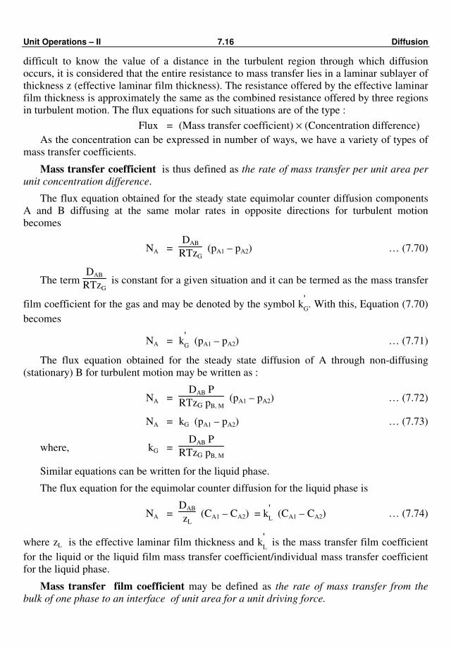
Unit Operations – II 7.16 Diffusion
difficult to know the value of a distance in the turbulent region through which diffusion
occurs, it is considered that the entire resistance to mass transfer lies in a laminar sublayer of
thickness z (effective laminar film thickness). The resistance offered by the effective laminar
film thickness is approximately the same as the combined resistance offered by three regions
in turbulent motion. The flux equations for such situations are of the type :
Flux = (Mass transfer coefficient) × (Concentration difference)
As the concentration can be expressed in number of ways, we have a variety of types of
mass transfer coefficients.
Mass transfer coefficient is thus defined as the rate of mass transfer per unit area per
unit concentration difference.
The flux equation obtained for the steady state equimolar counter diffusion components
A and B diffusing at the same molar rates in opposite directions for turbulent motion
becomes
NA = DAB
RTzG (pA1 – pA2) … (7.70)
The term DAB
RTzG is constant for a given situation and it can be termed as the mass transfer
film coefficient for the gas and may be denoted by the symbol k'G. With this, Equation (7.70)
becomes
NA = k'G (pA1 – pA2) … (7.71)
The flux equation obtained for the steady state diffusion of A through non-diffusing
(stationary) B for turbulent motion may be written as :
NA = DAB P
RTzG pB, M (pA1 – pA2) … (7.72)
NA = kG (pA1 – pA2) … (7.73)
where, kG = DAB P
RTzG pB, M
Similar equations can be written for the liquid phase.
The flux equation for the equimolar counter diffusion for the liquid phase is
NA = DAB
zL (CA1 – CA2) = k
'L (CA1 – CA2) … (7.74)
where zL is the effective laminar film thickness and k'L is the mass transfer film coefficient
for the liquid or the liquid film mass transfer coefficient/individual mass transfer coefficient
for the liquid phase.
Mass transfer film coefficient may be defined as the rate of mass transfer from the
bulk of one phase to an interface of unit area for a unit driving force.

Unit Operations – II 7.17 Diffusion
The flux equations for transfer of A through non-transferring B (i.e., diffusion of A
through non-diffusing B) in terms of the driving force expressed in terms of concentration
and molefraction are :
NA = ky (yA1 – yA2), NA = kC (CA1 – CA2) for gases … (7.75)
NA = kx (xA1 – xA2), NA = kL (CA1 – CA2) for liquids … (7.76)
Similar equations for equimolecular counter diffusion are :
NA = k'y (yA1 – yA2), NA = k
'c (CA1 – CA2) for gases … (7.77)
NA = k'x (xA1 – xA2), NA = k
'c (CA1 – CA2) for liquids … (7.78)
In two film concepts, z is the effective thickness of the film.
Relation between film coefficients :
Gases : k'c
P
RT = k
'c C = kc
pB, M
RT = k
'G P = k
'y = kv yB, m = kG pB, M = kG yB, M · P
pB, M = (pB1 – pB2)/ln (pB1 / pB2) , yB, M = (yB1 – yB2)/ln (yB1 / yB2),
Liquids : k'L C = k
'L ρ/M = k
'c C = k
'x = kx xB, M = kL xB, M C
Overall Mass Transfer Coefficient :
The overall mass transfer coefficients are measured on the basis of the gas phase or the
liquid phase driving force.
The flux equation in terms of the overall mass transfer coefficient and the overall driving
force for diffusion of A through non-diffusion B is given by
NA = KG (pA – p*A) … (7.79)
KG is the overall gas phase mass transfer coefficient in kmol/(m2⋅s) and (pA – p
*A) is the
overall driving force for the gas phase in terms of partial pressure.
p*A is the partial pressure of solute A over the solution having a composition of the bulk
liquid of CA. (Partial pressure of A in the gas phase that would be in equilibrium with CA, the
concentration of A in the bulk liquid phase.)
The flux can also be written as :
NA = Ky (yA – y*A) … (7.80)
Similarly,
NA = KL (C*A – CA) … (7.81)
where KL is the overall liquid phase mass transfer coefficient and is based on the
concentration difference driving force for the liquid phase. C*A is the concentration of solute
A in the liquid phase that would be in equilibrium with pA, partial pressure of A in the bulk
gas phase.
Mass transfer (film) coefficients in terms of the driving force in each phase are given by
NA = kG (pA – pAi) = kL (CAi – CA) … (7.82)
The overall driving force for the gas phase is
pA – p*A = (pA – pAi) + (pAi – p
*A ) … (7.83)
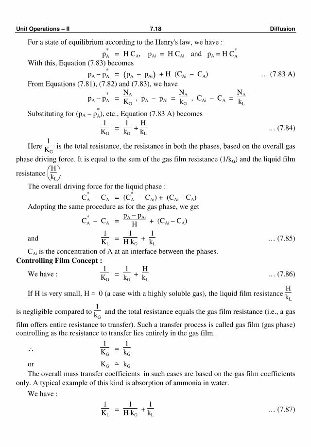
Unit Operations – II 7.18 Diffusion
For a state of equilibrium according to the Henry's law, we have :
p*A = H CA, pAi = H CAi and pA = H C
*A
With this, Equation (7.83) becomes
pA – p*A = ( )pA – pAi + H (CAi – CA) … (7.83 A)
From Equations (7.81), (7.82) and (7.83), we have
pA – p*A =
NA
KG , pA – pAi =
NA
kG , CAi – CA =
NA
kL
Substituting for (pA – p*A), etc., Equation (7.83 A) becomes
1
KG =
1
kG +
H
kL … (7.84)
Here 1
KG is the total resistance, the resistance in both the phases, based on the overall gas
phase driving force. It is equal to the sum of the gas film resistance (1/kG) and the liquid film
resistance
H
kL.
The overall driving force for the liquid phase :
C*A – CA = (C
*A – CAi) + (CAi – CA)
Adopting the same procedure as for the gas phase, we get
C*A – CA =
pA – pAi
H + (CAi – CA)
and 1
KL =
1
H kG +
1
kL … (7.85)
CAi is the concentration of A at an interface between the phases.
Controlling Film Concept :
We have : 1
KG =
1
kG +
H
kL … (7.86)
If H is very small, H –~ 0 (a case with a highly soluble gas), the liquid film resistance H
kL
is negligible compared to 1
kG and the total resistance equals the gas film resistance (i.e., a gas
film offers entire resistance to transfer). Such a transfer process is called gas film (gas phase)
controlling as the resistance to transfer lies entirely in the gas film.
∴ 1
KG =
1
kG
or KG –~ kG
The overall mass transfer coefficients in such cases are based on the gas film coefficients
only. A typical example of this kind is absorption of ammonia in water.
We have :
1
KL =
1
H kG +
1
kL … (7.87)
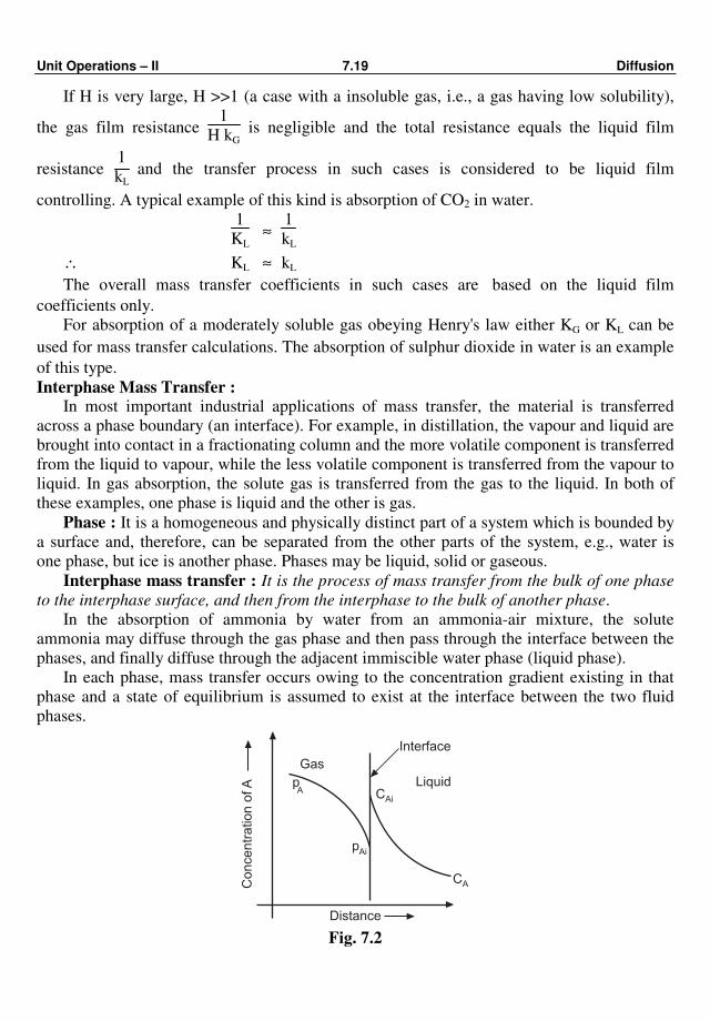
Unit Operations – II 7.19 Diffusion
If H is very large, H >>1 (a case with a insoluble gas, i.e., a gas having low solubility),
the gas film resistance 1
H kG is negligible and the total resistance equals the liquid film
resistance 1
kL and the transfer process in such cases is considered to be liquid film
controlling. A typical example of this kind is absorption of CO2 in water.
1
KL ≈
1
kL
∴ KL ≈ kL
The overall mass transfer coefficients in such cases are based on the liquid film
coefficients only.
For absorption of a moderately soluble gas obeying Henry's law either KG or KL can be
used for mass transfer calculations. The absorption of sulphur dioxide in water is an example
of this type.
Interphase Mass Transfer : In most important industrial applications of mass transfer, the material is transferred
across a phase boundary (an interface). For example, in distillation, the vapour and liquid are
brought into contact in a fractionating column and the more volatile component is transferred
from the liquid to vapour, while the less volatile component is transferred from the vapour to
liquid. In gas absorption, the solute gas is transferred from the gas to the liquid. In both of
these examples, one phase is liquid and the other is gas.
Phase : It is a homogeneous and physically distinct part of a system which is bounded by
a surface and, therefore, can be separated from the other parts of the system, e.g., water is
one phase, but ice is another phase. Phases may be liquid, solid or gaseous.
Interphase mass transfer : It is the process of mass transfer from the bulk of one phase
to the interphase surface, and then from the interphase to the bulk of another phase.
In the absorption of ammonia by water from an ammonia-air mixture, the solute
ammonia may diffuse through the gas phase and then pass through the interface between the
phases, and finally diffuse through the adjacent immiscible water phase (liquid phase).
In each phase, mass transfer occurs owing to the concentration gradient existing in that
phase and a state of equilibrium is assumed to exist at the interface between the two fluid
phases.
Interface
LiquidCAi
CA
pAi
pA
Gas
Concentr
ation o
fA
Distance
Fig. 7.2
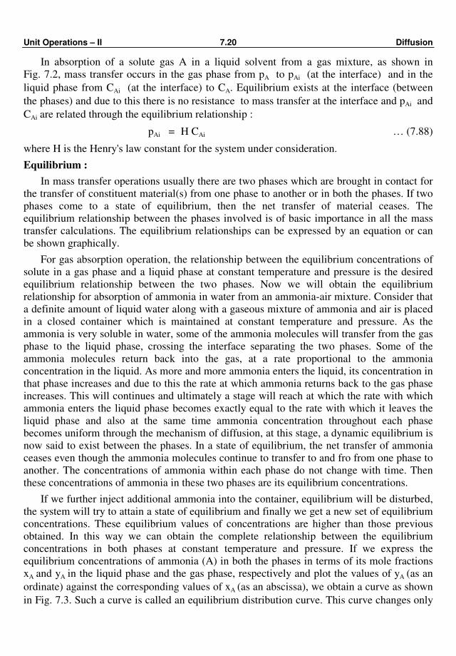
Unit Operations – II 7.20 Diffusion
In absorption of a solute gas A in a liquid solvent from a gas mixture, as shown in
Fig. 7.2, mass transfer occurs in the gas phase from pA to pAi (at the interface) and in the
liquid phase from CAi (at the interface) to CA. Equilibrium exists at the interface (between
the phases) and due to this there is no resistance to mass transfer at the interface and pAi and
CAi are related through the equilibrium relationship :
pAi = H CAi … (7.88)
where H is the Henry's law constant for the system under consideration.
Equilibrium :
In mass transfer operations usually there are two phases which are brought in contact for
the transfer of constituent material(s) from one phase to another or in both the phases. If two
phases come to a state of equilibrium, then the net transfer of material ceases. The
equilibrium relationship between the phases involved is of basic importance in all the mass
transfer calculations. The equilibrium relationships can be expressed by an equation or can
be shown graphically.
For gas absorption operation, the relationship between the equilibrium concentrations of
solute in a gas phase and a liquid phase at constant temperature and pressure is the desired
equilibrium relationship between the two phases. Now we will obtain the equilibrium
relationship for absorption of ammonia in water from an ammonia-air mixture. Consider that
a definite amount of liquid water along with a gaseous mixture of ammonia and air is placed
in a closed container which is maintained at constant temperature and pressure. As the
ammonia is very soluble in water, some of the ammonia molecules will transfer from the gas
phase to the liquid phase, crossing the interface separating the two phases. Some of the
ammonia molecules return back into the gas, at a rate proportional to the ammonia
concentration in the liquid. As more and more ammonia enters the liquid, its concentration in
that phase increases and due to this the rate at which ammonia returns back to the gas phase
increases. This will continues and ultimately a stage will reach at which the rate with which
ammonia enters the liquid phase becomes exactly equal to the rate with which it leaves the
liquid phase and also at the same time ammonia concentration throughout each phase
becomes uniform through the mechanism of diffusion, at this stage, a dynamic equilibrium is
now said to exist between the phases. In a state of equilibrium, the net transfer of ammonia
ceases even though the ammonia molecules continue to transfer to and fro from one phase to
another. The concentrations of ammonia within each phase do not change with time. Then
these concentrations of ammonia in these two phases are its equilibrium concentrations.
If we further inject additional ammonia into the container, equilibrium will be disturbed,
the system will try to attain a state of equilibrium and finally we get a new set of equilibrium
concentrations. These equilibrium values of concentrations are higher than those previous
obtained. In this way we can obtain the complete relationship between the equilibrium
concentrations in both phases at constant temperature and pressure. If we express the
equilibrium concentrations of ammonia (A) in both the phases in terms of its mole fractions
xA and yA in the liquid phase and the gas phase, respectively and plot the values of yA (as an
ordinate) against the corresponding values of xA (as an abscissa), we obtain a curve as shown
in Fig. 7.3. Such a curve is called an equilibrium distribution curve. This curve changes only
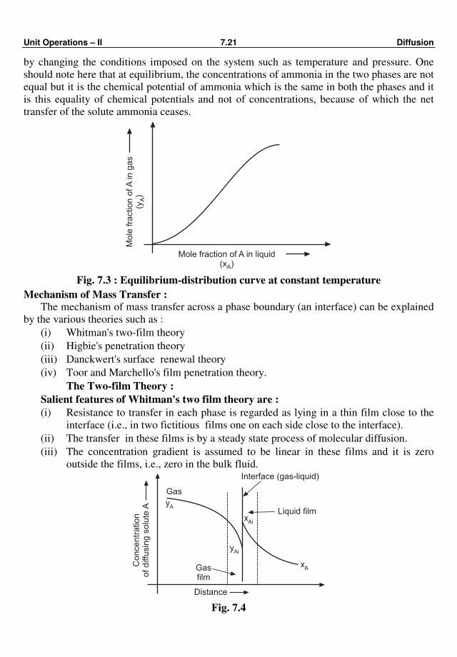
Unit Operations – II 7.21 Diffusion
by changing the conditions imposed on the system such as temperature and pressure. One
should note here that at equilibrium, the concentrations of ammonia in the two phases are not
equal but it is the chemical potential of ammonia which is the same in both the phases and it
is this equality of chemical potentials and not of concentrations, because of which the net
transfer of the solute ammonia ceases.
Mole fraction of A in liquid(x )A
Mo
le f
ractio
n o
fA
in g
as
(y)
A
Fig. 7.3 : Equilibrium-distribution curve at constant temperature
Mechanism of Mass Transfer : The mechanism of mass transfer across a phase boundary (an interface) can be explained
by the various theories such as :
(i) Whitman's two-film theory
(ii) Higbie's penetration theory
(iii) Danckwert's surface renewal theory
(iv) Toor and Marchello's film penetration theory.
The Two-film Theory :
Salient features of Whitman's two film theory are :
(i) Resistance to transfer in each phase is regarded as lying in a thin film close to the
interface (i.e., in two fictitious films one on each side close to the interface).
(ii) The transfer in these films is by a steady state process of molecular diffusion.
(iii) The concentration gradient is assumed to be linear in these films and it is zero
outside the films, i.e., zero in the bulk fluid. Interface (gas-liquid)
Liquid film
yAi
Gas
Co
nce
ntr
atio
no
f d
iffu
sin
g s
olu
teA
Distance
yA
xAi
Gasfilm
xA
Fig. 7.4

Unit Operations – II 7.22 Diffusion
(iv) The theory assumes that the turbulence in the bulk fluid vanishes at the interface of
the films.
(v) The film capacity is negligible, i.e., the time taken for a concentration gradient to
establish is small compared to the time of transfer.
Consider a solute gas (A) diffusing from a gas phase into a liquid phase. There must be a
concentration gradient in the direction of mass transfer within each phase. This is shown in
Fig. 7.4 graphically in terms of distance through the phases.
The concentration of A in the bulk of gas phase is yA molefraction, and it falls to yAi at
the interface. The concentration of A in the liquid phase falls from xAi at the interface
between the phases to xA in the bulk liquid. The bulk concentrations yA and xA are not in
equilibrium because otherwise the solute will not be diffused from the gas to the liquid
phase.
Whitman assumed that the resistance to transfer of A lies in two hypothetical films, one
on each side of the interface, in which the transfer is entirely by molecular diffusion. There is
no resistance to transfer across the interface and as a result the concentrations
yAi and xAi are the equilibrium values.
For steady state mass transfer, the rate of transfer of A to the interface must be equal to
the rate at which A is transferred from the interface to the bulk of liquid phase so that there is
no accumulation or depletion of A at the interface.
Therefore, we can write the mass transfer flux of A or rate of transfer of A in terms of
mass transfer coefficients and concentration changes occurring in the phases involved.
NA = ky (yA – yAi)
= kx (xAi – xA) … (7.89)
The differences in y's and x's are the driving forces for mass transfer.
Rearranging Equation (7.89), we get
kx
ky =
yA – yAi
xAi – xA … (7.90)
yA – yAi
xA – xAi = –
kx
ky … (7.91)
Fig. 7.5 shows typical values of the concentrations of the bulk phases (P) and at the
interface (Q).
Concentr
ation
of solu
teA
in g
as
yA
yAi
yA*
P
Q
xA xAi
Slope =– k
kx
y
Equilibrium curve = f(x )yAi Ai
Concentrationof solute A in liquid
Fig. 7.5

Unit Operations – II 7.23 Diffusion
In experimental determinations of the rate of transfer of the solute A, it is possible to
measure only the bulk concentrations of the solute A and to measure the interface
concentrations is ordinarily impossible. The equilibrium-distribution curve shown in Fig. 7.5
is unique at fixed T and P, so y*A in equilibrium with xA is a good measure of xA. Therefore,
the entire two phase mass transfer effects can be measured in terms of overall mass transfer
coefficient, Ky, i.e., the rate of mass transfer can also be set equal to the overall coefficient Ky
times the driving force ( )yA – y*A , where y
*A is the composition of the solute A in the gas
phase which is in equilibrium with xA.
NA = Ky ( )yA – y*A … (7.92)
1
Ky =
yA – y*A
NA =
(yA – yAi) + (yAi – y*A)
NA
1
Ky =
yA – yAi
NA +
yAi – y*A
NA
1
Ky =
1
ky +
yAi – y*A
kx (xAi – xA)
1
Ky =
1
ky +
m
kx … (7.93)
where, m = slope = ( )yAi – y*A / ( )xAi – xA
1/Ky is the overall resistance to mass transfer and 1/ky and m/kx are the resistances in the
liquid and gas films. The resistances in two phases are added to get an overall resistance and
hence it is also called as two resistance theory.
On the similar line, x*A is a measure of yA and it can be easily shown that
1
Kx =
1
m ky +
1
kx … (7.94)
The Penetration Theory :
The penetration theory was proposed by Higbie. The main features of this theory are :
1. As the time of exposure of fluid for mass transfer generally being short,
development/establishment of the concentration gradient of the film theory (the
characteristic of a steady state) is not possible.
2. The transfer is largly because of fresh material brought to the interface by the eddies.
3. A process of unsteady state transfer occurs for a fixed period at the freshly exposed
surface.
4. Each fluid element (eddy) resides for the same length of time period at the surface.
According to this theory, the mass transfer coefficient is proportional to the square
root of the diffusivity.

Unit Operations – II 7.24 Diffusion
Surface Renewal Theory :
According to this theory (proposed by Danckwerts) :
1. The eddies of the fluid at the surface are exposed to varying lengths of time.
2. On the basis of exposure-time histories, an age distribution for the surface elements is
calculated.
3. The mass transfer coefficient is proportional to the square root of the diffusivity
regardless of the nature of the surface renewal rate.
Counter current and Cocurrent Mass Transfer : Mass transfer processes that involve two fluid streams are frequently carried out
continuously by passing the fluid streams either in a counter current or a cocurrent fashion in
a column or device. The average driving force for a given situation will be larger in the
countercurrent operation than in the cocurrent operation and because of which a smaller size
equipment is needed for a given set of flow conditions for the countercurrent operation and
thus, the counter current flow is more common.
Examples of counter current mass transfer processes are :
(i) Distillation in packed column : In this case, a vapour stream (thermally created) is
moving up against the downward flow of a liquid reflux. At steady state, a state of
dynamic equilibrium is set up. The more volatile component under the action of a
concentration gradient is transferred from the liquid phase to the interface and then
from the interface into the vapour phase. The less volatile component is transferred
in the opposite direction and passes through the vapour into the liquid. Here
equimolar counter diffusion takes place since the molar latent heats of vaporisation
of two components are essentially the same.
(ii) Absorption in packed column : In this case, a solute gas together with a carrier
gas moves up against the downward flow of a liquid (solvent). The solute gas
diffuses through the gas phase to the interface where it dissolves and is then
transferred into the bulk of the liquid.
(iii) Liquid-liquid extraction in packed/spray column : In this case, both the streams
are liquid. The lighter liquid rises through the denser one. The solute diffuses from
the raffinate phase to the interface and away from the interface into the extract
phase.
Examples of Cocurrent Flow :
The cocurrent flow of gas and liquid streams usually in the downward direction through a
packed column is used for – catalytic chemical reaction between components of fluids,
diffusional operation when a gas to be dissolved in a liquid is a pure substance and for
diffusional operation accompanying a chemical reaction, e.g., in the absorption of hydrogen
sulfide in a sodium hydroxide solution. The cocurrent flow produces a separation effect
equivalent to that obtained with only one theoretical stage so used for such cases only. With
cocurrent flow there is no flooding and there is no upper limit for permissible phase flow
rates. The cocurrent flow is rarely used in the absence of a chemical reaction.
Analogies among Heat, Mass and Momentum Transfer :
Depending upon the fluid flow conditions, the mechanism of transfer process can be
classified as molecular transport (characteristic of stream line flow) and combined molecular
and eddy transfer (characteristic of total flow regime). There are similarities in governing

Unit Operations – II 7.25 Diffusion
equations for molecular transport as well as for turbulent transport and we can say that we
have analogies among these transport processes. A great deal of effort has been taken in
developing analogies (similarities) among these three transport processes for turbulent
transfer.
General Molecular Transport Equation :
The molecular transport of momentum, heat and mass is characterised by the same
general equation of the type :
Rate of a transfer process = Driving force
Resistance … (7.95)
Molecular transport or molecular diffusion equations for momentum, heat and
mass transfer :
These equations are applicable to laminar flow as molecular transport is a characteristic
of laminar/stream line flow.
Newton's law for momentum transport, i.e., Newton's equation for molecular diffusion
of momentum for constant density is
τzx = – µ
ρ
d (ux ρ)
dz … (7.96)
τzx = – ν d (ux ρ)
dz … (7.97)
where τzx is the momentum transferred per unit time per unit area, where the momentum has
the units of (kg.m)/s. [It is also called as the momentum flux], µ is viscosity and ρ is the
density of fluid. ν is the kinematic viscosity and also called as the diffusivity of momentum
and has the units of m2/s.
Fourier's law for heat transport, i.e., Fourier's equation for molecular diffusion of heat
for constant ρ and Cp is
qz
A = – α
d (ρ CpT)
dz … (7.98)
where qz
A is the heat transferred per unit time per unit area and is called as heat flux and has
the units of W/m2 [J/(m2.s)]. α is the thermal diffusivity or diffusivity of heat in m2/s.
Fick's law of molecular mass transport or Fick's equation for molecular diffusion of mass
for constant total concentration in a fluid is
JAz = – DAB dCA
dz
= – DAB d(ρA/MA)
dz … (7.99)
where JAz is the molar flux of component A in the z direction due to molecular diffusion in
kmol A/(m2.s), DAB is the molecular diffusivity of molecule A in B or mass diffusivity in
m2/s. CA is the molar concentration of A in kmol/m3.
Unit Operations – II 7.26 Diffusion
These three equation states, respectively, that (a) the momentum transport occurs
because of a gradient in momentum concentration, (b) the energy transport occurs because of
a gradient in energy concentration, and (c) the mass transport occurs because of a gradient in
mass concentration.
Turbulent diffusion equations for momentum, heat and mass transfer :
For combined molecular and eddy transfer, the relations for momentum, heat and mass
are :
For turbulent momentum transfer for constant density, we have
τzx = – (µ/ρ + εM) d(ux ρ)
dz … (7.100)
τzx = – (ν + εM) d (ρ ux)
dz … (7.101)
For turbulent heat transfer for constant ρ and Cp, we have
qz
A = – (α + εH)
d(ρ Cp T)
dz … (7.102)
For turbulent mass transfer for constant total molar concentration, we have
JAz = – (DAB + εD) dCA
dz … (7.103)
In the above equations, εm is the turbulent or eddy diffusivity of momentum in m2/s, εH is
the turbulent or eddy diffusivity of heat or eddy thermal diffusivity in m2/s and εM is the
turbulent or eddy diffusivity of mass in m2/s. Again, these equations are quite similar or
analogous to each other.
Equations (7.97), (7.98) and (7.99) for momentum, heat and mass transfer are similar to
each other and to the general molecular transport Equation (7.95). All these equations have a
flux on the left hand side which is momentum, heat or mass transferred per unit time per unit
area and a diffusivity of momentum, heat and mass (i.e., transport properties, ν, α and DAB)
all in m2/s, and a derivative of the concentration of a property with respect to the distance on
the right hand side. In all the above cases, the flux is proportional to the driving force. These
three molecular transport equations are mathematically identical. Thus, we say that we have
an analogy or similarity among them. Even though there is a mathematical analogy among
them, the actual physical mechanisms occurring is totally different.
The mass diffusivity DAB, the kinematic viscosity, ν and thermal diffusivity, α are
analogous as seen from the above equations.
The similarity in nature of transfer of these three processes are referred to as analogy.
Considering similarities between the governing equations of heat, mass and momentum
transfer, it is to be expected that the correlations for heat transfer coefficients and mass
transfer coefficients would also be similar. Various quantitative relations are available to
describe the analogical behaviour. The simplest and oldest is due to Reynolds.
Unit Operations – II 7.27 Diffusion
The Reynolds Analogy :
Reynolds was first to note similarities in transport processes and relates turbulent
momentum and heat transfer.
The basic assumption of the Reynolds analogy is that the ratio of two molecular
diffusivities equals to that of two eddy diffusivities.
ν
α = NPr =
εM
εH
… (7.104)
For turbulent flow conditions, the Reynolds analogy equations are :
The statement of Reynolds analogy between heat and momentum transfer is :
h
Cp u ρ =
h
Cp G = NSt =
f
2 … (7.105)
The statement of Reynolds analogy between mass and momentum transfer is :
k
'c
u =
f
2 … (7.106)
Therefore, the complete Reynolds analogy is
h
Cp u ρ =
k'c
u =
f
2 … (7.107)
NSt = NStm =
f
2 … (7.108)
where f is the Fanning friction factor (a measure of skin friction), u is the average velocity of
fluid, k'c is the convective mass transfer coefficient, h is the convective heat transfer
coefficient.
Equation (7.107) agrees well with the experimental data (correlates data) for gases in
turbulent flow if the Schmidt and Prandtl numbers are about unity and only the skin friction
is present in a flow past a flat plate or inside pipe. The equations do not correlate the data for
liquids in turbulent flow nor for any fluids in laminar flow, i.e., in such cases the analogy is
not valid.
Although the Reynolds analogy is of limited utility, the significant conclusion that may
be drawn is the mechanisms for momentum, heat and mass are identical at NPr = NSc = 1.0.
If a measure of the skin friction, i.e., the fanning friction factor is known, the analogy
may be used to find the heat transfer coefficient from the mass transfer coefficient and
vice-versa.
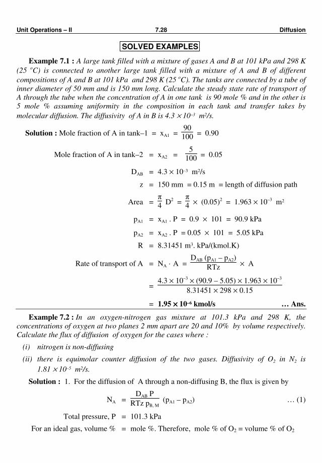
Unit Operations – II 7.28 Diffusion
SOLVED EXAMPLES
Example 7.1 : A large tank filled with a mixture of gases A and B at 101 kPa and 298 K
(25 oC) is connected to another large tank filled with a mixture of A and B of different
compositions of A and B at 101 kPa and 298 K (25 oC). The tanks are connected by a tube of
inner diameter of 50 mm and is 150 mm long. Calculate the steady state rate of transport of
A through the tube when the concentration of A in one tank is 90 mole % and in the other is
5 mole % assuming uniformity in the composition in each tank and transfer takes by
molecular diffusion. The diffusivity of A in B is 4.3 × 10⁻³ m2/s.
Solution : Mole fraction of A in tank–1 = xA1 = 90
100 = 0.90
Mole fraction of A in tank–2 = xA2 = 5
100 = 0.05
DAB = 4.3 × 10⁻³ m2/s
z = 150 mm = 0.15 m = length of diffusion path
Area = π
4 D2 =
π
4 × (0.05)2 = 1.963 × 10⁻³ m2
pA1 = xA1 . P = 0.9 × 101 = 90.9 kPa
pA2 = xA2 . P = 0.05 × 101 = 5.05 kPa
R = 8.31451 m3. kPa/(kmol.K)
Rate of transport of A = NA · A = DAB (pA1 – pA2)
RTz × A
= 4.3 × 10–3 × (90.9 – 5.05) × 1.963 × 10–3
8.31451 × 298 × 0.15
= 1.95 ×××× 10–6 kmol/s … Ans.
Example 7.2 : In an oxygen-nitrogen gas mixture at 101.3 kPa and 298 K, the
concentrations of oxygen at two planes 2 mm apart are 20 and 10% by volume respectively.
Calculate the flux of diffusion of oxygen for the cases where :
(i) nitrogen is non-diffusing
(ii) there is equimolar counter diffusion of the two gases. Diffusivity of O2 in N2 is
1.81 × 10⁻⁵ m2/s.
Solution : 1. For the diffusion of A through a non-diffusing B, the flux is given by
NA = DAB P
RTz pB, M (pA1 – pA2) … (1)
Total pressure, P = 101.3 kPa
For an ideal gas, volume % = mole %. Therefore, mole % of O2 = volume % of O2
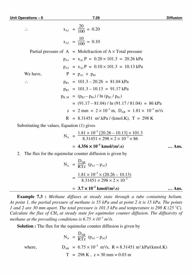
Unit Operations – II 7.29 Diffusion
∴ xA1 = 20
100 = 0.20
xA2 = 10
100 = 0.10
Partial pressure of A = Molefraction of A × Total pressure
pA1 = xA1 P = 0.20 × 101.3 = 20.26 kPa
pA2 = xA2 P = 0.10 × 101.3 = 10.13 kPa
We have, P = pA1 + pB1
∴ pB1 = 101.3 – 20.26 = 81.04 kPa
pB2 = 101.3 – 10.13 = 91.17 kPa
pB, M = (pB2 – pB1) / ln (pB2 / pB1)
= (91.17 – 81.04) / ln (91.17 / 81.04) = 86 kPa
z = 2 mm = 2 × 10⁻³ m, DAB = 1.81 × 10⁻⁵ m2/s
R = 8.31451 m3.kPa / (kmol.K), T = 298 K
Substituting the values, Equation (1) gives
NA = 1.81 × 10⁻⁵ [20.26 – 10.13] × 101.3
8.31451 × 298 × 2 × 10–3 × 86
= 4.356 ×××× 10–5 kmol/(m2.s) … Ans.
2. The flux for the equimolar counter diffusion is given by
NA = DAB
RTz (pA1 – pA2)
= 1.81 × 10–5 × (20.26 – 10.13)
8.31451 × 298 × 2 × 10–3
= 3.7 ×××× 10–5 kmol/(m2.s) … Ans.
Example 7.3 : Methane diffuses at steady state through a tube containing helium.
At point 1, the partial pressure of methane is 55 kPa and at point 2 it is 15 kPa. The points
1 and 2 are 30 mm apart. The total pressure is 101.3 kPa and temperature is 298 K (25 oC).
Calculate the flux of CH4 at steady state for equimolar counter diffusion. The diffusivity of
methane at the prevailing conditions is 6.75 × 10⁻⁵
m2/s.
Solution : The flux for the equimolar counter diffusion is given by
NA = DAB
RTz (pA1 – pA2)
where, DAB = 6.75 × 10⁻⁵ m2/s, R = 8.31451 m3.kPa/(kmol.K)
T = 298 K , z = 30 mm = 0.03 m

Unit Operations – II 7.30 Diffusion
pA1 = 55 kPa, pA2 = 15 kPa
NA = 6.75 × 10⁻⁵ (55 – 15)
8.31451 × 298 × 0.03
= 3.63 ×××× 10–5 kmol / (m2.s) … Ans.
Example 7.4 : Ammonia gas (A) diffuses through a non-diffusing nitrogen gas (B) under
steady state conditions. The partial pressure of A at location 1 is 1.5 × 10⁴ Pa and that at
location 2 is 5 × 10³ Pa (Pascal). The locations 1 and 2 are 0.15 m apart. The total pressure
is 1.103 × 10⁵ Pa and temperature is 298 K. Calculate the flux of diffusion of ammonia. Also
calculate the flux of diffusion for equimolar counter diffusion considering that nitrogen is
also diffusing. The diffusivity of ammonia at the prevailing conditions is 2.30 × 10⁻⁵
m2/s.
Solution : 1. The flux equation for the diffusion of A through a non-diffusing B is
given by
NA = DAB P
RTz pB, M (pA1 – pA2)
where DAB = 2.30 × 10⁻⁵ m2/s
P = 1.103 × 10⁵ Pa
pA1 = 1.5 × 10⁴ Pa
pA2 = 5 × 10³ Pa
pB1 = P – pA1 = 1.103 × 10⁵ – 1.5 × 104 = 8.63 × 10⁴ Pa
pB2 = P – pA2 = 1.103 × 10⁵ – 5 × 103 = 9.63 × 10⁴ Pa
pB, M = pB2 – pB1
ln (pB2 / pB1)
= (9.63 × 10⁴ – 8.63 × 10⁴)
ln (9.63 × 10⁴/8.63 × 104)
= 9.121 × 10⁴ Pa
T = 298 K, z = 0.15 m
R = 8.31451 m3. kPa/(kmol.K) = 8314.51 m3.Pa / (kmol.K)
NA = 2.30 × 10–5 × 1.103 × 105 (1.5 × 10⁴ – 5 × 10³)
8314.51 × 298 × 0.15 × 9.121 × 104
= 7.484 ×××× 10–7 kmol/(m2.s) … Ans.
2. The flux equation for the equimolar counter diffusion is given by
NA = DAB
RTz (pA1 – pA2)
= 2.30 × 10⁻⁵ (1.5 × 10⁴ – 5 × 10³)
8314.51 × 298 × 0.15
= 6.19 ×××× 10–7 kmol/(m2.s) … Ans.

Unit Operations – II 7.31 Diffusion
Example 7.5 : Hydrochloric acid (A) at 283 K diffuses through a thin film of water (B).
The film is 4 mm thick. The concentration of A at location 1, on one boundary of the film, is
12 weight % (density ρ1 = 1060.7 kg/m3) and at location 2, on the other boundary, is
4 weight % (density ρ2 = 1020.15 kg/m3). The diffusivity of HCl in water is 2.5 × 10⁻⁹
m2/s.
Calculate the flux of diffusion of A assuming water to be stagnant (i.e., non-diffusing).
Solution : Molecular weight of HCl = 36.5, Molecular weight of H2O = 18
At location 1 : Mole fraction of HCl (A)
xA1 = 12/36.5
12/36.5 + (100 – 12)/18
= 0.063
We have : xA1 + xB1 = 1
∴ xB1 = 1 – 0.063
= 0.937
Average molecular weight at location-1 is
M1 = 100
12/36.5 + (100 – 12)/18
= 19.166 kg/kmol
OR : In 100 kg of HCl – water mixture, there are 12 kg of HCl and 100 – 12 = 88 kg of H2O
at location-1 (as at location-1, HCl concentration is 12 weight %).
moles of HCl = 12
36.5 = 0.3287 kmol, moles of H2O =
88
18 = 4.8888 kmol
Total moles of the mixture = 0.3287 + 4.8888 = 5.2175 kmol
∴ xA1 = Moles of HCl
Total moles =
0.3287
5.2175 = 0.063
M1 = kg of mixture / kmol of mixture
= 100
5.2175 = 19.166 kg/kmol
At location–2, the molefraction of HCl is
xA2 = 4/36.5
(4/36.5) + (100 – 4)/18
= 0.1096
0.1096 + 5.3333 = 0.0201
xB2 = 1 – 0.0201
= 0.9799
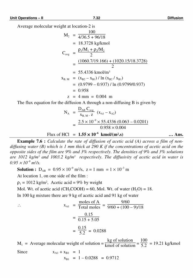
Unit Operations – II 7.32 Diffusion
Average molecular weight at location-2 is
M2 = 100
4/36.5 + 96/18
= 18.3728 kg/kmol
Cavg = ρ1/M1 + ρ2/M2
2
= (1060.7/19.166) + (1020.15/18.3728)
2
= 55.4336 kmol/m3
xB, M = (xB2 – xB1) / ln (xB2 / xB1)
= (0.9799 – 0.937) / ln (0.9799/0.937)
= 0.958
z = 4 mm = 0.004 m
The flux equation for the diffusion A through a non-diffusing B is given by
NA = DAB Cavg
xB, M . z (xA1 – xA2)
= 2.5 × 10–9 × 55.4336 (0.063 – 0.0201)
0.958 × 0.004
Flux of HCl = 1.55 ×××× 10–6 kmol/(m2.s) … Ans.
Example 7.6 : Calculate the rate of diffusion of acetic acid (A) across a film of non-
diffusing water (B) which is 1 mm thick at 290 K if the concentrations of acetic acid on the
opposite sides of the film are 9% and 3% respectively. The densities of 9% and 3% solutions
are 1012 kg/m3 and 1003.2 kg/m3 respectively. The diffusivity of acetic acid in water is
0.95 × 10⁻⁹
m2/s.
Solution : DAB = 0.95 × 10⁻⁹ m2/s, z = 1 mm = 1 × 10⁻³ m
At location 1, on one side of the film :
ρ1 = 1012 kg/m2, Acetic acid = 9% by weight
Mol. Wt. of acetic acid (CH3COOH) = 60, Mol. Wt. of water (H2O) = 18.
In 100 kg mixture there are 9 kg of acetic acid and 91 kg of water
∴ xA1 = moles of A
Total moles =
9/60
9/60 + (100 – 9)/18
= 0.15
0.15 + 5.05
= 0.15
5.2 = 0.0288
M1 = Average molecular weight of solution = kg of solution
kmol of solution =
100
5.2 = 19.21 kg/kmol
Since xA1 + xB1 = 1
xB1 = 1 – 0.0288 = 0.9712
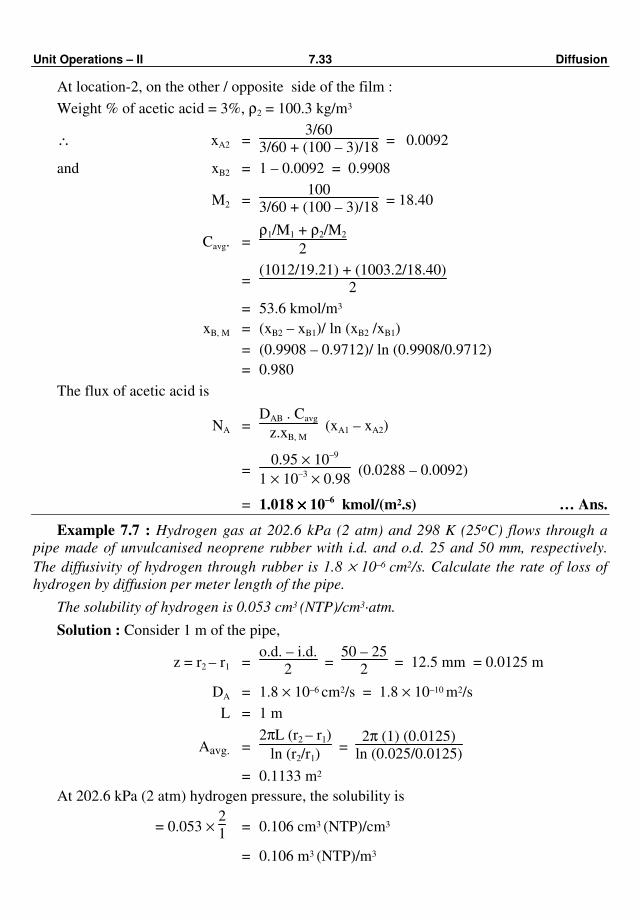
Unit Operations – II 7.33 Diffusion
At location-2, on the other / opposite side of the film :
Weight % of acetic acid = 3%, ρ2 = 100.3 kg/m3
∴ xA2 = 3/60
3/60 + (100 – 3)/18 = 0.0092
and xB2 = 1 – 0.0092 = 0.9908
M2 = 100
3/60 + (100 – 3)/18 = 18.40
Cavg. = ρ1/M1 + ρ2/M2
2
= (1012/19.21) + (1003.2/18.40)
2
= 53.6 kmol/m3
xB, M = (xB2 – xB1)/ ln (xB2 /xB1)
= (0.9908 – 0.9712)/ ln (0.9908/0.9712)
= 0.980
The flux of acetic acid is
NA = DAB . Cavg
z.xB, M (xA1 – xA2)
= 0.95 × 10⁻⁹
1 × 10–3 × 0.98 (0.0288 – 0.0092)
= 1.018 ×××× 10–6 kmol/(m2.s) … Ans.
Example 7.7 : Hydrogen gas at 202.6 kPa (2 atm) and 298 K (25oC) flows through a
pipe made of unvulcanised neoprene rubber with i.d. and o.d. 25 and 50 mm, respectively.
The diffusivity of hydrogen through rubber is 1.8 × 10⁻⁶ cm2/s. Calculate the rate of loss of
hydrogen by diffusion per meter length of the pipe.
The solubility of hydrogen is 0.053 cm3 (NTP)/cm3·atm.
Solution : Consider 1 m of the pipe,
z = r2 – r1 = o.d. – i.d.
2 =
50 – 25
2 = 12.5 mm = 0.0125 m
DA = 1.8 × 10⁻⁶ cm2/s = 1.8 × 10⁻¹⁰ m2/s
L = 1 m
Aavg. = 2πL (r2 – r1)
ln (r2/r1) =
2π (1) (0.0125)
ln (0.025/0.0125)
= 0.1133 m2
At 202.6 kPa (2 atm) hydrogen pressure, the solubility is
= 0.053 × 2
1 = 0.106 cm3 (NTP)/cm3
= 0.106 m3 (NTP)/m3

Unit Operations – II 7.34 Diffusion
∴ CA1 at the inner surface of the pipe = 0.106
22.4 × 1 = 4.73 × 10⁻³ kmol H2/m3
At the outer surface, CA2 = 0
The rate of loss of hydrogen per 1 m length of the pipe is
w = NA · Aavg. = DA · Aavg. [CA1 – CA2]/z
= 1.8 × 10–10 × 0.1133 (4.73 × 10⁻³ – 0)/0.0125
= 7.72 ×××× 10–2 kmol H2/s per m … Ans.
Some Important Definitions :
1. Gram mole : It is defined as the mass in grams of a substance that is numerically
equal to its molecular weight.
In this book, gram mole and kilogram mole are specified as mol and kmol respectively.
2. Weight fraction : It is the ratio of the weight of the individual component to
the total weight of the system. It is denoted by the symbol x'.
For two component system : x'A + x
'B = 1.0.
Weight % of A = Weight fraction of A × 100
3. Mole fraction : It is the ratio of the moles of the individual component to the total
moles of the system. It is denoted by the symbol x.
For a binary system of A and B : xA + xB = 1.0.
Mole % of A = mole fraction of A × 100.
4. More volatile component : It is the component with a lower boiling point or with a
higher vapour pressure at a given temperature (in a binary system). It is also called as the
lighter component.
In case of distillation, the compositions of vapour and liquid phases are expressed in
terms of mole fraction of the more volatile component.
5. Less volatile component : In a binary system, it is the component with a higher
boiling point or with a lower vapour pressure at a given temperature. It is also called as the
heavier component.
6. Vapour pressure : The vapour pressure of a liquid is defined as the absolute
pressure at which the liquid and its vapour are in equilibrium at a given temperature.
7. Partial pressure : The partial pressure of a component gas that is present in a
mixture of gases in the pressure that would be exerted by that component if it alone were
present in the same volume and at the same temperature as the mixture.
8. Ideal gas law : The ideal gas law is given by
PV = nRT
if P is in kPa, V in m3, n in kmol and T in K then R will be in m3·kPa/(kmol·K).
R (universal gas constant) = 8.31451 m3 · kPa/(kmol·K)
Unit Operations – II 7.35 Diffusion
9. Dalton's law : Mathematically, Dalton's law is given by
P = pA + pB + pC + …
where P is the total pressure exerted by a gas mixture and pA, pB, pC … are the partial
pressures of component gases A, B, C, …. present in the mixture.
10. Raoult's law : It states that the equilibrium partial pressure of component A is equal
to the product of the vapour pressure and the mole fraction of A in the liquid phase.
∴ pA = p0
A · xA
pA is also related to yA by the following equation
pA = yA · P
yA is the mole fraction of A in the gas phase.
11. Henry's law : Mathematically Henry's law is given as,
pA = H xA
where H is the Henry's law constant.
Henry's law expresses the relationship between the concentration of a gas dissolved in a
liquid and the equilibrium partial pressure of the gas above the liquid surface.
12. Gibb's phase rule : It is the relationship that governs all heterogeneous equilibria. It
is given by
F = C – P + 2
where C = number of components
P = number of phases
F is the number of degrees of freedom or number of intensive variables (temperature,
pressure, composition) that must be specified so that remaining variables will be fixed
automatically and the system will be defined completely.
EXERCISES
1. Give the mathematical statement of Fick's law of diffusion and give the meaning of
each terms involved in it.
2. Define :
(i) Mass fraction,
(ii) Mole fraction,
(iii) Molar concentration,
(iv) Mass average velocity, and
(v) Molar average velocity.
3. Define : Mass flux and Molar flux and give the expressions for Mass and Molar
fluxes relative to the mass average velocity and molar average velocity.
Unit Operations – II 7.36 Diffusion
4. Define Diffusion, Molecular diffusion, Eddy/turbulent diffusion and explain briefly
the role of diffusion in mass transfer.
5. Explain briefly analogy between heat, mass and momentum.
6. Explain briefly Reynolds analogy.
7. Show that for equimolar counter diffusion, DAB = DBA.
8. State the Fick's law of diffusion.
9. Give the mathematical expression for analogy between heat, mass and momentum
transport for laminar and turbulent flow. Give the meaning of each term.
10. Define mass transfer coefficient. Give its SI unit.
11. What do you mean by interphase mass transfer ?
12. State salient features of two-film theory.
13. Explain the controlling film concept.
ppp
(8.1)
CHAPTER EIGHT
DISTILLATION
Distillation is a unit operation in which the constituents of a liquid mixture (solution)
are separated using thermal energy. Basically, the difference in vapour pressures
(volatilities) of different constituents at the same temperature is responsible for such a
separation. This unit operation is also termed as fractional distillation or fractionation.
With this technique it is possible to separate the liquid mixture into its components in almost
pure form and due to this distillation is the most important of all the mass transfer operations.
In distillation, the phases involved are : liquid and vapour (the vapour phase is created by
supplying heat to the liquid) and mass is transferred from both the phases to one another, by
vaporisation from the liquid phase and by condensation from the vapour phase. The net effect
is an increase in composition of the more volatile component in the vapour (phase) and that
of the less volatile component in the liquid. The basic requirement for a separation of
components by distillation is that the composition of the vapour be different from the
composition of the liquid with which it is in equilibrium - the vapour is always richer in the
more volatile component than the liquid from which it is formed. If the vapour composition
is the same as the liquid composition, distillation technique will not effect a separation.
Distillation is commonly used in chemical and petroleum industries as a means of
separating the liquid mixture into its component parts. Separation of ethanol and water
mixture, production of absolute alcohol from 95% ethanol using benzene, separation of
petroleum crude into gasoline, kerosene, fuel oils, etc. are the typical examples of
distillation.
Evaporation is concerned with the separation of a solution containing a non-volatile
solute and a volatile solvent, whereas distillation is concerned with the separation of solution
where all the components are appreciably volatile. Thus, the separation of a brine into salt
and water is a evaporation, whereas the separation of a mixture of alcohol and water into its
components is a distillation.
Boiling Point :
For any given pressure, a pure liquid when heated will boil or vaporise at a certain single
temperature known as the boiling point of the liquid. It is the temperature of a liquid at which
the vapour pressure of a liquid equals the prevailing pressure. The boiling point of a liquid
increases with increase in pressure and vice versa. The normal boiling of a liquid is the
temperature at which its boiling takes place under a pressure of 1 atm. Boiling points
at a given pressure vary greatly for different liquids. For example, the boiling point of
water is 373 K (100o C), that of toluene is 383.6 K (110.6o C) and that of methanol is
337.7 K (64.7o C) at one atmosphere (101.325 kPa).
Unit Operations – II 8.2 Distillation
In a binary mixture (a two component system), the component with a lower boiling point,
i.e., the component with a higher vapour pressure at a given temperature is termed as the
more volatile or lighter, while the component with a higher boiling point or with a lower
vapour pressure at a given temperature is termed as the less volatile or heavier.
Thus, in case of a binary mixture of methanol and water, methanol (B.P. = 64.7°C) is a
more volatile component and water (B.P. = 100°C) is a less volatile component, since the
vapour pressure of methanol is higher than that of water at any given temperature. The whole
mixture of methanol and water will boil somewhere between 337.7 K (64.7o C) and
373 K (100o C) at atmospheric pressure (101.325 kPa).
Vapour pressure :
The vapour pressure of a liquid is the pressure exerted by the vapour at equilibrium
condition – the conditions at which the rate of vaporisation equals the rate of condensation.
Equilibrium :
• It is a static condition in which the net transfer of material between the phases ceases
for a given set of operating conditions that exists for all combinations of phases.
• Equilibrium refers to the absence of any tendency for a change to take place and thus
represent an end point of any naturally occurring process.
Driving force :
When two phases, which are not at equilibrium are brought into intimate contact, the
phases will tend to approach equilibrium due to a tendency for change to take place. The
difference between the existing condition and equilibrium condition is the driving force
which causes a change. A concentration difference is the driving force for mass transfer
analogous to a temperature difference for heat transfer.
Equilibrium stage :
It is one in which the two phases not at equilibrium are brought into contact, time is
provided to attain equilibrium, the phases are separated and streams leave the stage in
equilibrium. For a given set of operating conditions, an equilibrium stage gives the maximum
possible composition change, so it is also known as the ideal or theoretical stage. In actual
practice, equilibrium is not achieved and hence stage efficiencies are always less than 100
percent.
Vapour - Liquid Equilibrium :
The basic data for distillation are the equilibria existing between the vapour and liquid
phases of a system under consideration. The equilibrium in vapour-liquid systems is
governed by phase rule. In a binary mixture subjected to distillation, we have :
C (components) = 2, P (phases) = 2. So, according to the phase rule [F = C – P + 2], the
degrees of freedom (F) or the number of intensive variables that must be fixed to define the
equilibrium state of the system (here F = 2). In distillation, there are four variables :
temperature, pressure, vapour phase composition and liquid phase composition. Thus, if the
pressure is fixed then only one variable say, for example, the liquid phase composition can be
changed independently and the temperature and vapour phase composition follow and thus
the system is completely defined.
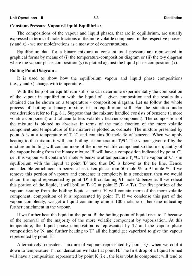
Unit Operations – II 8.3 Distillation
Constant-Pressure Vapour-Liquid Equilibria :
The compositions of the vapour and liquid phases, that are in equilibrium, are usually
expressed in terms of mole fractions of the more volatile component in the respective phases
(y and x) - we use molefractions as a measure of concentrations.
Equilibrium data for a binary mixture at constant total pressure are represented in
graphical forms by means of (i) the temperature-composition diagram or (ii) the x-y diagram
where the vapour phase composition (y) is plotted against the liquid phase composition (x).
Boiling Point Diagram :
It is used to show how the equilibrium vapour and liquid phase compositions
(i.e., y and x) change with temperature.
With the help of an equilibrium still one can determine experimentally the composition
of the vapour in equilibrium with the liquid of a given composition and the results thus
obtained can be shown on a temperature - composition diagram. Let us follow the whole
process of boiling a binary mixture in an equilibrium still. For the situation under
consideration refer to Fig. 8.1. Suppose that the mixture handled consists of benzene (a more
volatile component) and toluene (a less volatile / heavier component). The composition of
the mixture is plotted as abscissa in terms of the mole fraction of the more volatile
component and temperature of the mixture is plotted as ordinate. The mixture presented by
point A is at a temperature of T1oC and contains 50 mole % of benzene. When we apply
heating to the mixture it will start boiling at temperature T2oC. The vapour given off by the
mixture on boiling will contain more of the more volatile component so the first quantity of
the vapour issuing from the binary mixture 'B' will have a composition indicated by point 'C',
i.e., this vapour will contain 91 mole % benzene at temperature T2 oC. The vapour at 'C' is in
equilibrium with the liquid at point 'B' and thus BC is known as the tie line. Hence,
considerable enrichment in benzene has taken place from 50 mole % to 91 mole %. If we
remove this portion of vapours and condense it completely in a condenser, then we would
obtain the liquid represented by point 'D' still containing 91 mole % benzene. If we reheat
this portion of the liquid, it will boil at T3 oC at point E (T3 < T2). The first portion of the
vapours issuing from the boiling liquid at point 'E' will contain more of the more volatile
component, composition of it is represented by point 'F'. If we condense this part of the
vapour completely, we get a liquid containing almost 100 mole % of benzene indicating
further enrichment in the vapour.
If we further heat the liquid at the point 'B' the boiling point of liquid rises to T' because
of the removal of the majority of the more volatile component by vaporisation. At this
temperature, the liquid phase composition is represented by 'L' and the vapour phase
composition by 'N' and further heating to T" all the liquid get vaporised to give the vapour
represented by point 'H'.
Alternatively, consider a mixture of vapours represented by point 'Q', when we cool it
down to temperature T", condensation will start at point H. The first drop of a liquid formed
will have a composition represented by point K (i.e., the less volatile component will tend to
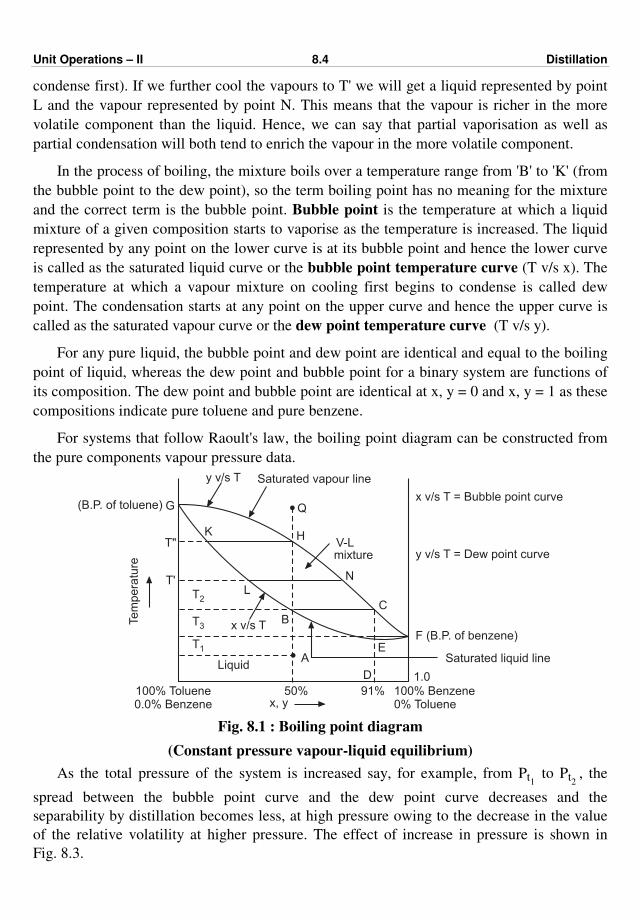
Unit Operations – II 8.4 Distillation
condense first). If we further cool the vapours to T' we will get a liquid represented by point
L and the vapour represented by point N. This means that the vapour is richer in the more
volatile component than the liquid. Hence, we can say that partial vaporisation as well as
partial condensation will both tend to enrich the vapour in the more volatile component.
In the process of boiling, the mixture boils over a temperature range from 'B' to 'K' (from
the bubble point to the dew point), so the term boiling point has no meaning for the mixture
and the correct term is the bubble point. Bubble point is the temperature at which a liquid
mixture of a given composition starts to vaporise as the temperature is increased. The liquid
represented by any point on the lower curve is at its bubble point and hence the lower curve
is called as the saturated liquid curve or the bubble point temperature curve (T v/s x). The
temperature at which a vapour mixture on cooling first begins to condense is called dew
point. The condensation starts at any point on the upper curve and hence the upper curve is
called as the saturated vapour curve or the dew point temperature curve (T v/s y).
For any pure liquid, the bubble point and dew point are identical and equal to the boiling
point of liquid, whereas the dew point and bubble point for a binary system are functions of
its composition. The dew point and bubble point are identical at x, y = 0 and x, y = 1 as these
compositions indicate pure toluene and pure benzene.
For systems that follow Raoult's law, the boiling point diagram can be constructed from
the pure components vapour pressure data.
N
C
G
T"
T'
Te
mp
era
ture
Saturated vapour liney v/s T
Q
HK
L
V-Lmixture
T2
T3
T1
x v/s TB
LiquidA
E
D 1.0
F (B.P. of benzene)
y v/s T = Dew point curve
x v/s T = Bubble point curve
Saturated liquid line
(B.P. of toluene)
100% Toluene0.0% Benzene
50% 91% 100% Benzene0% Toluenex, y
Fig. 8.1 : Boiling point diagram
(Constant pressure vapour-liquid equilibrium)
As the total pressure of the system is increased say, for example, from Pt1 to Pt2 , the
spread between the bubble point curve and the dew point curve decreases and the
separability by distillation becomes less, at high pressure owing to the decrease in the value
of the relative volatility at higher pressure. The effect of increase in pressure is shown in
Fig. 8.3.
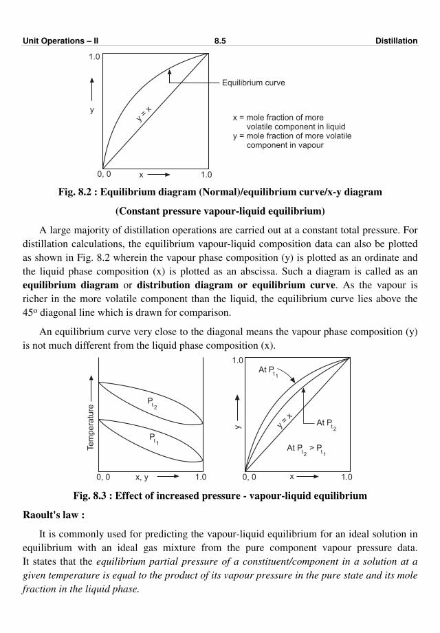
Unit Operations – II 8.5 Distillation
y
1.0
0, 0 1.0
y =
x
x
Equilibrium curve
x = mole fraction of morevolatile component in liquid
y = mole fraction of more volatilecomponent in vapour
Fig. 8.2 : Equilibrium diagram (Normal)/equilibrium curve/x-y diagram
(Constant pressure vapour-liquid equilibrium)
A large majority of distillation operations are carried out at a constant total pressure. For
distillation calculations, the equilibrium vapour-liquid composition data can also be plotted
as shown in Fig. 8.2 wherein the vapour phase composition (y) is plotted as an ordinate and
the liquid phase composition (x) is plotted as an abscissa. Such a diagram is called as an
equilibrium diagram or distribution diagram or equilibrium curve. As the vapour is
richer in the more volatile component than the liquid, the equilibrium curve lies above the
45o diagonal line which is drawn for comparison.
An equilibrium curve very close to the diagonal means the vapour phase composition (y)
is not much different from the liquid phase composition (x).
0, 0 1.0x, y
Tem
pera
ture
Pt2
Pt1
0, 0 1.0x
1.0At P
t1
At Pt2y y
= x
At P > Pt2 t1
Fig. 8.3 : Effect of increased pressure - vapour-liquid equilibrium
Raoult's law :
It is commonly used for predicting the vapour-liquid equilibrium for an ideal solution in
equilibrium with an ideal gas mixture from the pure component vapour pressure data.
It states that the equilibrium partial pressure of a constituent/component in a solution at a
given temperature is equal to the product of its vapour pressure in the pure state and its mole
fraction in the liquid phase.

Unit Operations – II 8.6 Distillation
Thus, for a binary (two component) system, if pA is the equilibrium partial pressure of A,
poA is the vapour pressure of 'A' in the pure state and xA is the mole fraction of 'A' in the
liquid phase, then
pA = poA xA … (8.1)
and pB = poB xB … (8.2)
= poB (1 – xA) as xA + xB = 1
pB = equilibrium partial pressure of B
xB = mole fraction of B in liquid phase
poB = vapour pressure of pure B.
Dalton's Law :
It states that the total pressure exerted by a gas/vapour mixture is equal to the sum of the
partial pressures of the components present in it. Thus, it expresses the additive nature of the
partial pressures.
Mathematically, for a binary system :
P = pA + pB … (8.3)
where P is the total pressure.
For an ideal gas or vapour, the partial pressure is related to mole fraction of the
component in gas or vapour phase by the relation :
Partial pressure = Mole fraction × Total pressure
Thus, for component 'A'
pA = yA · P … (8.4)
where yA is the mole fraction of 'A' in the vapour phase.
Knowing the vapour pressures of components 'A' (more volatile component) and 'B' at
various values of temperatures, x - y data can be generated for an ideal solution as follows :
pA = poA · xA … (8.5)
pB = poB · (1 – xA) … (8.6)
pA = yA · P … (8.7)
pB = yB · P … (8.8)
From Equations (8.5) and (8.7), we get
poA · xA = yA · P … (8.9)
yA = p
oA
P · xA … (8.10)
Similarly, yB = p
oB
P · xB … (8.11)
We have, yB + yB = 1 and xB = 1 – xA
yA + yB = 1

Unit Operations – II 8.7 Distillation
Substituting for yA and yB from Equations (8.10) and (8.11), and xB in terms of xA, the
above equation becomes
p
oA
P · xA +
poB
P (1 – xA) = 1 … (8.12)
poA · xA + p
oB – p
oB · xA = P … (8.13)
∴ xA ( )poA – p
oB = P – p
oB … (8.14)
Rearranging gives
xA = P – p
oB
poA – p
oB
… (8.15)
Knowing xA, the corresponding equilibrium value of the vapour phase concentration (yA)
is obtained with the help of Equation (8.10).
Relative volatility :
Volatility of A : It is defined as the ratio of the partial pressure of 'A' to the mole
fraction of 'A' in the liquid phase.
Volatility of A = pA
xA … (8.16)
Similarly, Volatility of B = pB
xB … (8.17)
The relative volatility of a component A with respect to a component B is the ratio of the
volatility of 'A' (the more volatile component) to the volatility of 'B'. It is also known as the
volatility of 'A' with respect to 'B' and is denoted by the symbol αAB.
∴ αAB = pA xB
xA · pB … (8.18)
but PyA = pA and PyB = pB
∴ αAB = yA · xB
yB · xA … (8.19)
αAB = yA / yB
xA / xB … (8.20)
Thus, the relative volatility is the ratio of the concentration ratio of A to B in the vapour
phase to that in the liquid phase.
αAB = yA xB
yB · xA
We have, yB = 1 – yA … (8.21)
xB = 1 – xA … (8.22)
∴ αAB = yA (1 – xA)
(1 – yA) · xA … (8.23)

Unit Operations – II 8.8 Distillation
αAB (1 – yA) xA = yA (1 – xA)
αAB xA – αAB yA xA = yA – yA xA
αAB · xA = yA + yA xA (αAB – 1)
αAB xA = yA [1 + (αAB – 1) xA] … (8.24)
∴ yA = αAB · xA
1 + (αAB – 1) xA
… (8.25)
Dropping subscripts, we get
y = αx
1 + (α – 1) x … (8.26)
From the above equation knowing 'α' for a given binary system x – y data (equilibrium
data) can be generated by taking x = 0, 0.1 …… to 1 and evaluating the corresponding values
of 'y' (equilibrium vapour phase composition).
For an ideal system, volatility is equal to the vapour pressure of the pure component.
The relative volatility of A with respect to B is also defined as the ratio of the vapour
pressure of A to the vapour pressure of B at the same temperature. Therefore,
Relative volatility = αAB = p
oA
poB
… (8.27)
Relative volatility is a measure of the separability by distillation (i.e., it is a measure of
the ease with which the components are separated). When αααα = 1, separation by distillation is
not possible. The separation by distillation is possible for relative volatility values greater
than one. Larger the value of the relative volatility, the easier is the separation by distillation.
METHODS OF DISTILLATION - BINARY SYSTEMS :
Basically, distillation is carried out in two ways :
1. The liquid mixture to be separated is heated to create a vapour. The vapour formed is
condensed in a condenser and withdrawn as product. As there is no reflux, products
of relatively low purities are obtained.
2. The liquid mixture to be separated is heated to create a vapour, the vapour formed is
condensed in a condenser. A part of the condensed liquid is returned to the
distillation still (as reflux) and the remaining part is withdrawn as product. In this
method, the liquid and vapour are brought into intimate contact for a number of times
and almost pure product can be achieved. The part of the condensed liquid returned
to the distillation unit is called reflux and the operation is called rectification or
fractionation. The term rectification originated in the alcohol industry, whereas the
term fractionation is popular in the petroleum industry.
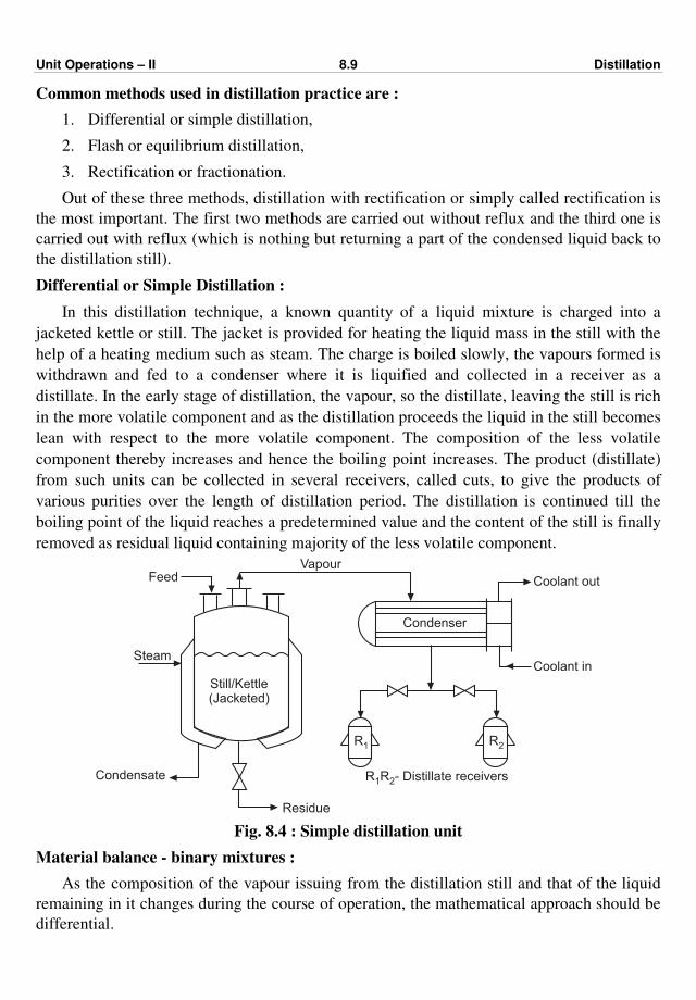
Unit Operations – II 8.9 Distillation
Common methods used in distillation practice are :
1. Differential or simple distillation,
2. Flash or equilibrium distillation,
3. Rectification or fractionation.
Out of these three methods, distillation with rectification or simply called rectification is
the most important. The first two methods are carried out without reflux and the third one is
carried out with reflux (which is nothing but returning a part of the condensed liquid back to
the distillation still).
Differential or Simple Distillation :
In this distillation technique, a known quantity of a liquid mixture is charged into a
jacketed kettle or still. The jacket is provided for heating the liquid mass in the still with the
help of a heating medium such as steam. The charge is boiled slowly, the vapours formed is
withdrawn and fed to a condenser where it is liquified and collected in a receiver as a
distillate. In the early stage of distillation, the vapour, so the distillate, leaving the still is rich
in the more volatile component and as the distillation proceeds the liquid in the still becomes
lean with respect to the more volatile component. The composition of the less volatile
component thereby increases and hence the boiling point increases. The product (distillate)
from such units can be collected in several receivers, called cuts, to give the products of
various purities over the length of distillation period. The distillation is continued till the
boiling point of the liquid reaches a predetermined value and the content of the still is finally
removed as residual liquid containing majority of the less volatile component.
Still/Kettle(Jacketed)
Steam
Feed
Condensate
Residue
Vapour
Condenser
R1 R2
Coolant out
Coolant in
R R1 2- Distillate receivers
Fig. 8.4 : Simple distillation unit
Material balance - binary mixtures :
As the composition of the vapour issuing from the distillation still and that of the liquid
remaining in it changes during the course of operation, the mathematical approach should be
differential.
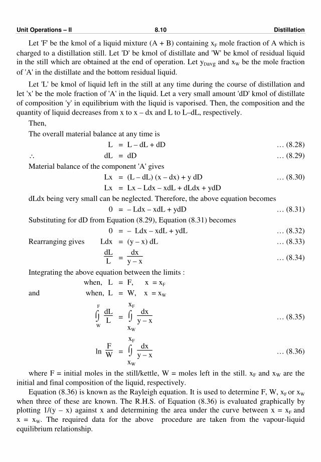
Unit Operations – II 8.10 Distillation
Let 'F' be the kmol of a liquid mixture (A + B) containing xF mole fraction of A which is
charged to a distillation still. Let 'D' be kmol of distillate and 'W' be kmol of residual liquid
in the still which are obtained at the end of operation. Let yDavg and xW be the mole fraction
of 'A' in the distillate and the bottom residual liquid.
Let 'L' be kmol of liquid left in the still at any time during the course of distillation and
let 'x' be the mole fraction of 'A' in the liquid. Let a very small amount 'dD' kmol of distillate
of composition 'y' in equilibrium with the liquid is vaporised. Then, the composition and the
quantity of liquid decreases from x to x – dx and L to L–dL, respectively.
Then,
The overall material balance at any time is
L = L – dL + dD … (8.28)
∴ dL = dD … (8.29)
Material balance of the component 'A' gives
Lx = (L – dL) (x – dx) + y dD … (8.30)
Lx = Lx – Ldx – xdL + dLdx + ydD
dLdx being very small can be neglected. Therefore, the above equation becomes
0 = – Ldx – xdL + ydD … (8.31)
Substituting for dD from Equation (8.29), Equation (8.31) becomes
0 = – Ldx – xdL + ydL … (8.32)
Rearranging gives Ldx = (y – x) dL … (8.33)
dL
L =
dx
y – x … (8.34)
Integrating the above equation between the limits :
when, L = F, x = xF
and when, L = W, x = xW
⌡⌠W
F
dL
L = ⌡⌠
xW
xF
dx
y – x … (8.35)
ln F
W = ⌡⌠
xW
xF
dx
y – x … (8.36)
where F = initial moles in the still/kettle, W = moles left in the still. xF and xW are the
initial and final composition of the liquid, respectively.
Equation (8.36) is known as the Rayleigh equation. It is used to determine F, W, xF or xW
when three of these are known. The R.H.S. of Equation (8.36) is evaluated graphically by
plotting 1/(y – x) against x and determining the area under the curve between x = xF and
x = xW. The required data for the above procedure are taken from the vapour-liquid
equilibrium relationship.
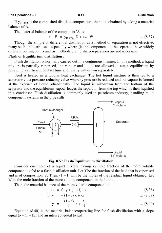
Unit Operations – II 8.11 Distillation
If yD, avg. is the composited distillate composition, then it is obtained by taking a material
balance of A.
The material balance of the component 'A' is
xF · F = yD, avg. D + xW · W … (8.37)
Though the simple or differential distillation as a method of separation is not effective,
many such units are used, especially where (i) the components to be separated have widely
different boiling points and (ii) methods giving sharp separations are not necessary.
Flash or Equilibrium distillation :
Flash distillation is normally carried out in a continuous manner. In this method, a liquid
mixture is partially vaporised, the vapour and liquid are allowed to attain equilibrium by
providing a sufficient contact time and finally withdrawn separately.
Feed is heated in a tubular heat exchanger. The hot liquid mixture is then fed to a
separator via a pressure reducing valve whereby pressure is reduced and the vapour is formed
at the expense of liquid adiabatically. The liquid is withdrawn from the bottom of the
separator and the equilibrium vapour leaves the separator from the top which is then liquified
in a condenser. Flash distillation is commonly used in petroleum industry, handling multi
component systems in the pipe stills.
Heat exchanger
Feed
1 molexF
P.R.V.
Vapour'f' mole, y
Separator
Liquid(1-f) mole, x
Fig. 8.5 : Flash/Equilibrium distillation
Consider one mole of a liquid mixture having xF mole fraction of the more volatile
component, is fed to a flash distillation unit. Let 'f be the fraction of the feed that is vaporised
and is of composition 'y'. Then, (1 – f) will be the moles of the residual liquid obtained. Let
'x' be the mole fraction of the more volatile component in the liquid.
Then, the material balance of the more volatile component is
xF = f · y + (1 – f) · x … (8.38)
f · y = – (1 – f) x + xF … (8.39)
y = – (1 – f)
f x +
xF
f … (8.40)
Equation (8.40) is the material balance/operating line for flash distillation with a slope
equal to – (1 – f)/f and an intercept equal to xF/f.
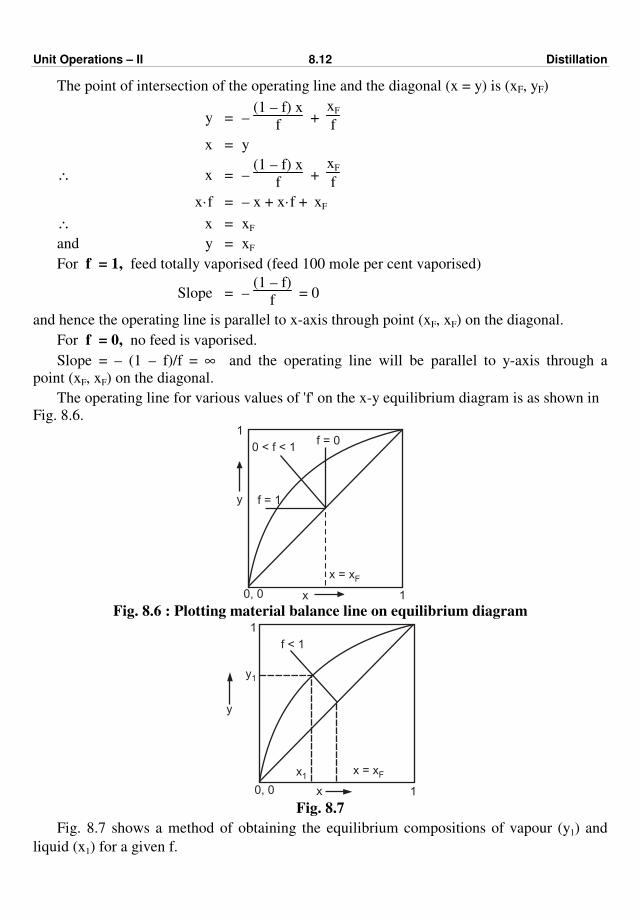
Unit Operations – II 8.12 Distillation
The point of intersection of the operating line and the diagonal (x = y) is (xF, yF)
y = – (1 – f) x
f +
xF
f
x = y
∴ x = – (1 – f) x
f +
xF
f
x·f = – x + x·f + xF
∴ x = xF
and y = xF
For f = 1, feed totally vaporised (feed 100 mole per cent vaporised)
Slope = – (1 – f)
f = 0
and hence the operating line is parallel to x-axis through point (xF, xF) on the diagonal.
For f = 0, no feed is vaporised.
Slope = – (1 – f)/f = ∞ and the operating line will be parallel to y-axis through a
point (xF, xF) on the diagonal.
The operating line for various values of 'f' on the x-y equilibrium diagram is as shown in
Fig. 8.6. 1
y f = 1
0, 0 x 1
x = xF
f = 00 < f < 1
Fig. 8.6 : Plotting material balance line on equilibrium diagram
y1
1
f < 1
y
x1x = xF
x 10, 0
Fig. 8.7
Fig. 8.7 shows a method of obtaining the equilibrium compositions of vapour (y1) and
liquid (x1) for a given f.
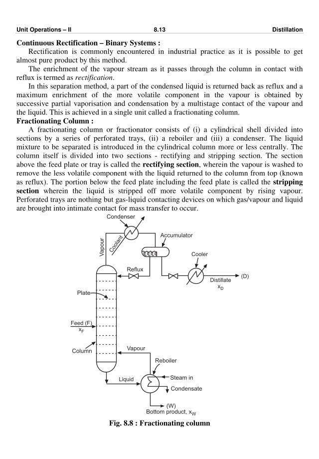
Unit Operations – II 8.13 Distillation
Continuous Rectification – Binary Systems : Rectification is commonly encountered in industrial practice as it is possible to get
almost pure product by this method.
The enrichment of the vapour stream as it passes through the column in contact with
reflux is termed as rectification.
In this separation method, a part of the condensed liquid is returned back as reflux and a
maximum enrichment of the more volatile component in the vapour is obtained by
successive partial vaporisation and condensation by a multistage contact of the vapour and
the liquid. This is achieved in a single unit called a fractionating column.
Fractionating Column : A fractionating column or fractionator consists of (i) a cylindrical shell divided into
sections by a series of perforated trays, (ii) a reboiler and (iii) a condenser. The liquid
mixture to be separated is introduced in the cylindrical column more or less centrally. The
column itself is divided into two sections - rectifying and stripping section. The section
above the feed plate or tray is called the rectifying section, wherein the vapour is washed to
remove the less volatile component with the liquid returned to the column from top (known
as reflux). The portion below the feed plate including the feed plate is called the stripping
section wherein the liquid is stripped off more volatile component by rising vapour.
Perforated trays are nothing but gas-liquid contacting devices on which gas/vapour and liquid
are brought into intimate contact for mass transfer to occur.
Feed (F)xF
Liquid
Vapour
Condenser
Accumulator
Reflux
Plate
Vapour
Reboiler
Steam in
Condensate
(W)Bottom product, xW
Column
Cooler
Coo
lant
(D)Distillate
xD
Fig. 8.8 : Fractionating column
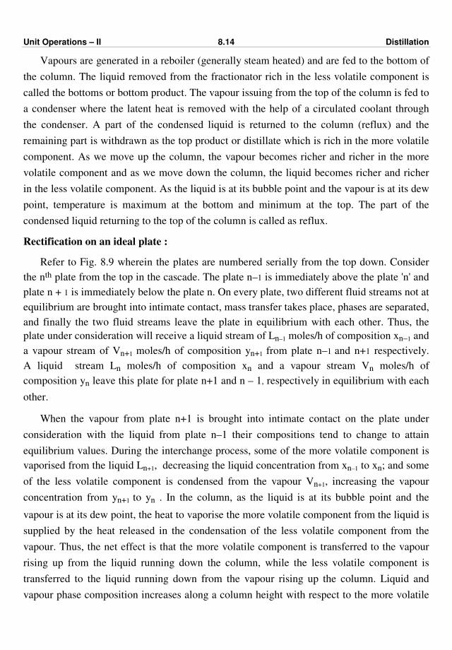
Unit Operations – II 8.14 Distillation
Vapours are generated in a reboiler (generally steam heated) and are fed to the bottom of
the column. The liquid removed from the fractionator rich in the less volatile component is
called the bottoms or bottom product. The vapour issuing from the top of the column is fed to
a condenser where the latent heat is removed with the help of a circulated coolant through
the condenser. A part of the condensed liquid is returned to the column (reflux) and the
remaining part is withdrawn as the top product or distillate which is rich in the more volatile
component. As we move up the column, the vapour becomes richer and richer in the more
volatile component and as we move down the column, the liquid becomes richer and richer
in the less volatile component. As the liquid is at its bubble point and the vapour is at its dew
point, temperature is maximum at the bottom and minimum at the top. The part of the
condensed liquid returning to the top of the column is called as reflux.
Rectification on an ideal plate :
Refer to Fig. 8.9 wherein the plates are numbered serially from the top down. Consider
the nth plate from the top in the cascade. The plate n–1 is immediately above the plate 'n' and
plate n + 1 is immediately below the plate n. On every plate, two different fluid streams not at
equilibrium are brought into intimate contact, mass transfer takes place, phases are separated,
and finally the two fluid streams leave the plate in equilibrium with each other. Thus, the
plate under consideration will receive a liquid stream of Ln–1 moles/h of composition xn–1 and
a vapour stream of Vn+1 moles/h of composition yn+1 from plate n–1 and n+1 respectively.
A liquid stream Ln moles/h of composition xn and a vapour stream Vn moles/h of
composition yn leave this plate for plate n+1 and n – 1, respectively in equilibrium with each
other.
When the vapour from plate n+1 is brought into intimate contact on the plate under
consideration with the liquid from plate n–1 their compositions tend to change to attain
equilibrium values. During the interchange process, some of the more volatile component is
vaporised from the liquid Ln+1, decreasing the liquid concentration from xn–1 to xn; and some
of the less volatile component is condensed from the vapour Vn+1, increasing the vapour
concentration from yn+1 to yn . In the column, as the liquid is at its bubble point and the
vapour is at its dew point, the heat to vaporise the more volatile component from the liquid is
supplied by the heat released in the condensation of the less volatile component from the
vapour. Thus, the net effect is that the more volatile component is transferred to the vapour
rising up from the liquid running down the column, while the less volatile component is
transferred to the liquid running down from the vapour rising up the column. Liquid and
vapour phase composition increases along a column height with respect to the more volatile
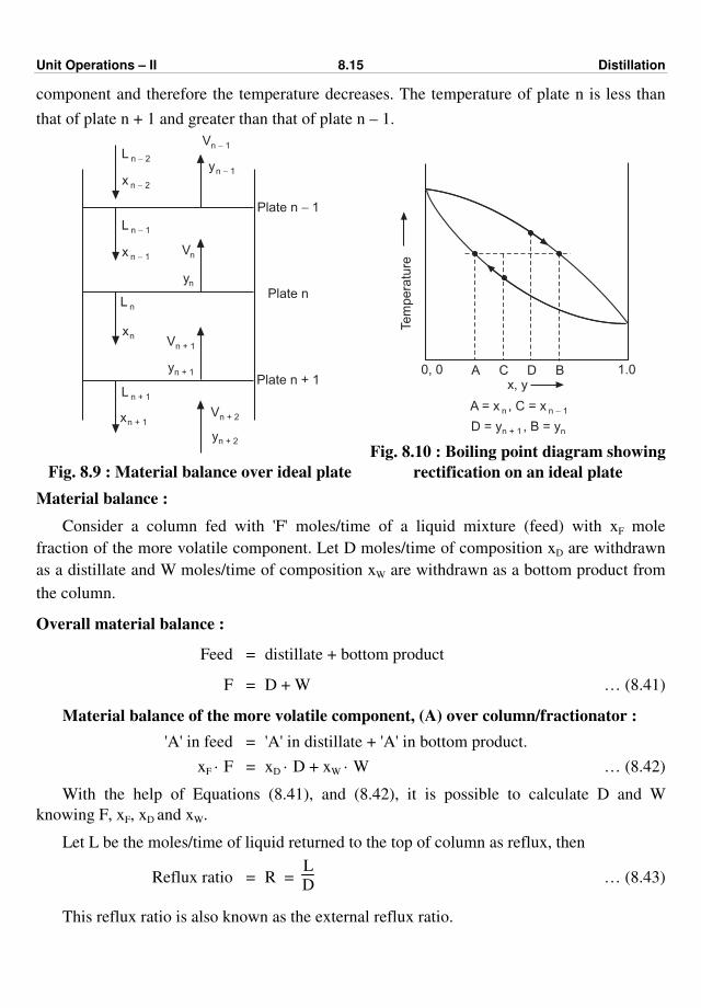
Unit Operations – II 8.15 Distillation
component and therefore the temperature decreases. The temperature of plate n is less than
that of plate n + 1 and greater than that of plate n – 1.
L n 2-
x n 2-
L n 1-
x n 1-
L n
xn
L n + 1
xn + 1
Vn + 1
yn + 1
Vn + 2
yn + 2
Vn 1-
yn 1-
Vn
yn
Plate n 1-
Plate n
Plate n + 1
Fig. 8.9 : Material balance over ideal plate
Tem
pera
ture
x, y0, 0 1.0A C D B
A = x , C = xn n 1-
D = y , = yn + 1 nB
Fig. 8.10 : Boiling point diagram showing
rectification on an ideal plate
Material balance :
Consider a column fed with 'F' moles/time of a liquid mixture (feed) with xF mole
fraction of the more volatile component. Let D moles/time of composition xD are withdrawn
as a distillate and W moles/time of composition xW are withdrawn as a bottom product from
the column.
Overall material balance :
Feed = distillate + bottom product
F = D + W … (8.41)
Material balance of the more volatile component, (A) over column/fractionator :
'A' in feed = 'A' in distillate + 'A' in bottom product.
xF · F = xD · D + xW · W … (8.42)
With the help of Equations (8.41), and (8.42), it is possible to calculate D and W
knowing F, xF, xD and xW.
Let L be the moles/time of liquid returned to the top of column as reflux, then
Reflux ratio = R = L
D … (8.43)
This reflux ratio is also known as the external reflux ratio.
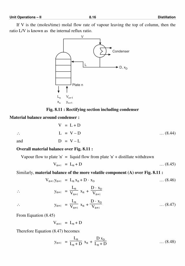
Unit Operations – II 8.16 Distillation
If V is the (moles/time) molal flow rate of vapour leaving the top of column, then the
ratio L/V is known as the internal reflux ratio.
Condenser
LD, xD
V
Plate n
Ln Vn+1
xn yn+1
Fig. 8.11 : Rectifying section including condenser
Material balance around condenser :
V = L + D
∴ L = V – D … (8.44)
and D = V – L
Overall material balance over Fig. 8.11 :
Vapour flow to plate 'n' = liquid flow from plate 'n' + distillate withdrawn
Vn+1 = Ln + D … (8.45)
Similarly, material balance of the more volatile component (A) over Fig. 8.11 :
Vn+1 yn+1 = Ln xn + D · xD … (8.46)
∴ yn+1 = Ln
Vn+1 xn +
D · xD
Vn+1
∴ yn+1 = Ln
Vn+1 xn +
D · xD
Vn+1 … (8.47)
From Equation (8.45)
Vn+1 = Ln + D
Therefore Equation (8.47) becomes
yn+1 = Ln
Ln + D xn +
D xD
Ln + D … (8.48)

Unit Operations – II 8.17 Distillation
Equation (8.48) is known as the material balance line or the operating line of the
rectifying section.
Reboiler
L', x'
V', y'
Plate m 1+
V , ym+1 m+1
W, xW
x , Lm m
Fig. 8.12 : Stripping section including reboiler
Overall material balance over Fig. 8.12 :
Liquid flow to plate – m + 1 = Vapour flow from plate – m + 1
+ Bottom product withdrawn
Lm = Vm+1 + W … (8.49)
Similarly,
Material balance of more volatile component (A) :
Lm · xm = Vm+1 ym +1 + W xW … (8.50)
Rearranging the equation (8.50)
ym+1 = Lm
Vm+1 xm –
WxW
Vm+1 … (8.51)
We know from equation (8.49), that Vm+1 = Lm – W.
∴ ym+1 = Lm
Lm – W xm –
WxW
Lm – W … (8.52)
Equation (8.52) is known as the material balance line or the operating line for the
stripping section.
Analysis of fractionating columns :
The theoretical/ideal stages/plates required for a given/specified degree of separation can
be obtained by :
1. McCabe – Thiele method.
2. Lewis – Sorel method.
McCabe – Thiele Method :
It is a graphical procedure of obtaining theoretical plates.
The assumptions made in this method are :
1. Constant molal heat of vaporisation.
2. No heat losses.
3. No heat of mixing.
Unit Operations – II 8.18 Distillation
The above cited assumptions leads to a concept of constant molal vapour flow and
constant molal liquid flow in any section of the column (i.e., the molal flow rates of vapour
and liquid are constant in any section of the column). In other words, for one mole of liquid
vaporised, one mole of vapour is condensed in any section (rectifying or stripping). Thus,
Vn = Vn+1, Ln = Ln+1 … etc.
The subscripts n, n + 1, m, m + 1 … etc. may be dropped and the operating lines then
plotted on the equilibrium diagram are straight.
Therefore, operating line for the rectifying section becomes
y = L
L + D x +
D xD
L + D … (8.53)
With R = L
D , Equation (8.53) becomes
y = R
R + 1 x +
xD
R + 1 … (8.54)
On the xy diagram, it is a straight line with a slope equal to R/(R + 1) and an intercept
equal to xD/(R + 1).
The point of intersection of the operating line for rectifying section and the diagonal y =
x is obtained as
y = R
R + 1 x +
xD
R + 1
Substituting y = x
∴ x = R
R + 1 x +
xD
R + 1
(R + 1) x = R · x + xD
∴ x = xD
and y = xD
Thus, the operating line of the rectifying section is to be drawn on the equilibrium
diagram through point (xD, xD) on the diagonal and with a slope equal to R/(R + 1) or an
intercept on the y-axis equal to xD/(R + 1).
The operating line of the stripping section by dropping the subscripts m, m + 1 becomes
y = L'
L' – W x –
W xW
L' – W … (8.55)
On the xy diagram, i.e., on the equilibrium diagram, it is a straight line with a slope of
L'/(L' – W) and an intercept of WxW/(L' – W).
The point of intersection of the operating line of the stripping section and the diagonal is
obtained as follows :
y = L'
L' – W x –
W xW
L – W
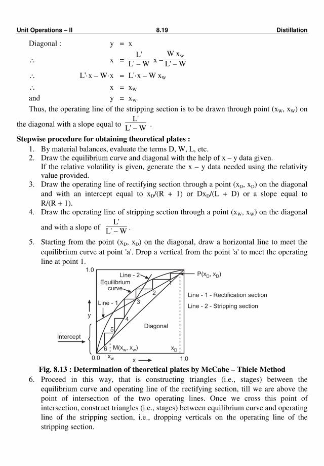
Unit Operations – II 8.19 Distillation
Diagonal : y = x
∴ x = L'
L' – W x –
W xw
L' – W
∴ L'·x – W·x = L'·x – W xW
∴ x = xW
and y = xW
Thus, the operating line of the stripping section is to be drawn through point (xW, xW) on
the diagonal with a slope equal to L'
L' – W .
Stepwise procedure for obtaining theoretical plates :
1. By material balances, evaluate the terms D, W, L, etc.
2. Draw the equilibrium curve and diagonal with the help of x – y data given.
If the relative volatility is given, generate the x – y data needed using the relativity
value provided.
3. Draw the operating line of rectifying section through a point (xD, xD) on the diagonal
and with an intercept equal to xD/(R + 1) or DxD/(L + D) or a slope equal to
R/(R + 1).
4. Draw the operating line of stripping section through a point (xW, xW) on the diagonal
and with a slope of L'
L' – W .
5. Starting from the point (xD, xD) on the diagonal, draw a horizontal line to meet the
equilibrium curve at point 'a'. Drop a vertical from the point 'a' to meet the operating
line at point 1.
y
x 1.0
1.0
4
3
2
1
5
M(x , x )w w
xw
xD
P(x , x )D D
Intercept
Line - 1 - Rectification section
Line - 2 - Stripping section
6
0.0
Diagonal
Line - 2
Line - 1
Equilibriumcurve
Fig. 8.13 : Determination of theoretical plates by McCabe – Thiele Method
6. Proceed in this way, that is constructing triangles (i.e., stages) between the
equilibrium curve and operating line of the rectifying section, till we are above the
point of intersection of the two operating lines. Once we cross this point of
intersection, construct triangles (i.e., stages) between equilibrium curve and operating
line of the stripping section, i.e., dropping verticals on the operating line of the
stripping section.
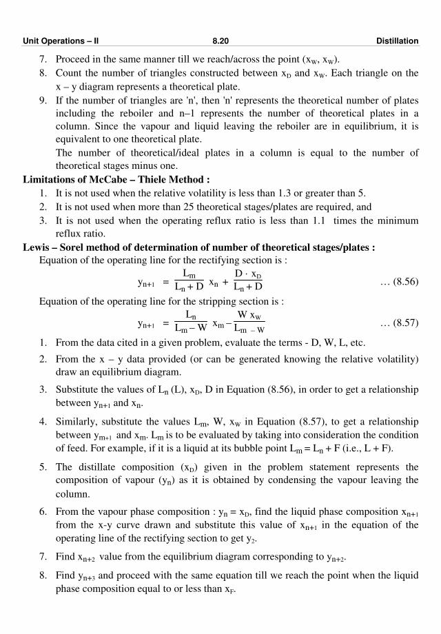
Unit Operations – II 8.20 Distillation
7. Proceed in the same manner till we reach/across the point (xW, xW).
8. Count the number of triangles constructed between xD and xW. Each triangle on the
x – y diagram represents a theoretical plate.
9. If the number of triangles are 'n', then 'n' represents the theoretical number of plates
including the reboiler and n–1 represents the number of theoretical plates in a
column. Since the vapour and liquid leaving the reboiler are in equilibrium, it is
equivalent to one theoretical plate.
The number of theoretical/ideal plates in a column is equal to the number of
theoretical stages minus one.
Limitations of McCabe – Thiele Method :
1. It is not used when the relative volatility is less than 1.3 or greater than 5.
2. It is not used when more than 25 theoretical stages/plates are required, and
3. It is not used when the operating reflux ratio is less than 1.1 times the minimum
reflux ratio.
Lewis – Sorel method of determination of number of theoretical stages/plates :
Equation of the operating line for the rectifying section is :
yn+1 = Lm
Ln + D xn +
D · xD
Ln + D … (8.56)
Equation of the operating line for the stripping section is :
yn+1 = Ln
Lm – W xm –
W xW
Lm – W … (8.57)
1. From the data cited in a given problem, evaluate the terms - D, W, L, etc.
2. From the x – y data provided (or can be generated knowing the relative volatility)
draw an equilibrium diagram.
3. Substitute the values of Ln (L), xD, D in Equation (8.56), in order to get a relationship
between yn+1 and xn.
4. Similarly, substitute the values Lm, W, xW in Equation (8.57), to get a relationship
between ym+1 and xm. Lm is to be evaluated by taking into consideration the condition
of feed. For example, if it is a liquid at its bubble point Lm = Ln + F (i.e., L + F).
5. The distillate composition (xD) given in the problem statement represents the
composition of vapour (yn) as it is obtained by condensing the vapour leaving the
column.
6. From the vapour phase composition : yn = xD, find the liquid phase composition xn+1
from the x-y curve drawn and substitute this value of xn+1 in the equation of the
operating line of the rectifying section to get y2.
7. Find xn+2 value from the equilibrium diagram corresponding to yn+2.
8. Find yn+3 and proceed with the same equation till we reach the point when the liquid
phase composition equal to or less than xF.
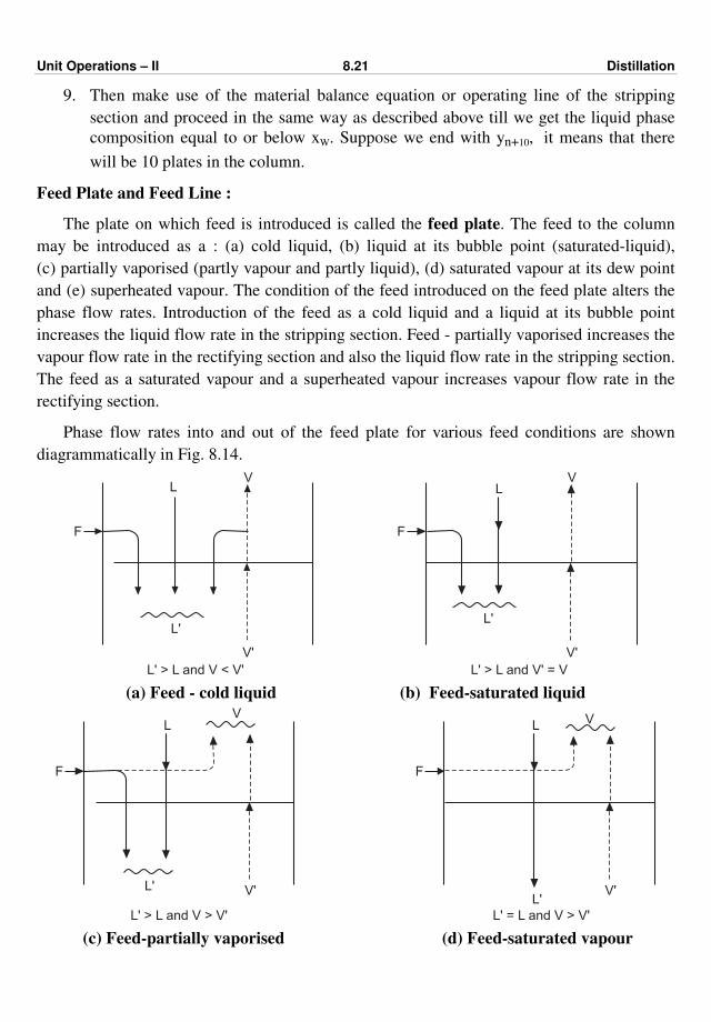
Unit Operations – II 8.21 Distillation
9. Then make use of the material balance equation or operating line of the stripping
section and proceed in the same way as described above till we get the liquid phase
composition equal to or below xW. Suppose we end with yn+10, it means that there
will be 10 plates in the column.
Feed Plate and Feed Line :
The plate on which feed is introduced is called the feed plate. The feed to the column
may be introduced as a : (a) cold liquid, (b) liquid at its bubble point (saturated-liquid),
(c) partially vaporised (partly vapour and partly liquid), (d) saturated vapour at its dew point
and (e) superheated vapour. The condition of the feed introduced on the feed plate alters the
phase flow rates. Introduction of the feed as a cold liquid and a liquid at its bubble point
increases the liquid flow rate in the stripping section. Feed - partially vaporised increases the
vapour flow rate in the rectifying section and also the liquid flow rate in the stripping section.
The feed as a saturated vapour and a superheated vapour increases vapour flow rate in the
rectifying section.
Phase flow rates into and out of the feed plate for various feed conditions are shown
diagrammatically in Fig. 8.14.
LV
L'
V'
L' > L and V' = V
F
LV
L'
V'
L' > L and V < V'
F
(a) Feed - cold liquid (b) Feed-saturated liquid
LV
L' V'
L' > L and V > V'
F
LV
L'V'
L' = L and V > V'
F
(c) Feed-partially vaporised (d) Feed-saturated vapour

Unit Operations – II 8.22 Distillation
L
L' V'
L' < L and V > V'
F
V
(e) Feed-superheated vapour
Fig. 8.14 : Flow through feed plate for various feed conditions
The phase flow rates shown are based on the fact that the column liquid is always at its
bubble point and vapour is always at its dew point. To calculate the change in phase flow
rates by the introduction of feed, a factor 'q' is introduced. The 'q' is a measure of the
thermal condition of the feed and is defined as the number of moles of saturated liquid
resulting in the stripping section for each mole of feed introduced. Thus for a feed F, we get :
L' = L + qF … (8.58)
and V = V' + (1 – q) F … (8.59)
The values of 'q' for various thermal conditions of the feed are :
(a) Cold liquid : q > 1
(b) Saturated liquid : q = 1
(c) Feed partially vapour (partially flashed, i.e., a vapour-liquid mixture) : 0 < q < 1
(d) Saturated vapour feed (feed at a dew point) : q = 0, and
(e) Superheated vapour feed : q < 0.
The value of q for any particular feed condition can be calculated from the following
relation.
q = Energy to convert 1 mole of feed to saturated vapour
Molal latent heat of vaporisation
The liquid flow in the stripping section is
L' = L + qF … (8.60)
∴ L' – L = qF … (8.61)
Similarly, the vapour flow in the rectifying section is
V = V' + (1 – q) F … (8.62)
∴ V – V' = (1 – q) F … (8.63)
V = L + D – (overall balance-upper section) … (8.64)
∴ Vy = Lx + DxD – (material balance of 'A') … (8.65)
and V' = L' – W – (overall balance-lower section) … (8.66)
V'y = L'x – WxW – (material balance of A) … (8.67)

Unit Operations – II 8.23 Distillation
Subtracting Equation (8.67) from Equation (8.65)
∴ y (V – V') = x (L – L') + D xD + W xW … (8.68)
But we know that :
xF·F = D·xD + W xW … (8.69)
∴ Equation (8.68) becomes
y (V – V') = x (L – L') + xF · F … (8.70)
Substituting the values of V – V' and L – L' from Equations (8.63) and (8.61) into
Equation (8.70) gives
y (1 – q) F = x (– qF) + xF·F … (8.71)
∴ y = – q
1 – q x +
xF
1 – q … (8.72)
Equation (8.72) is known as the feed line or q-line or q-line equation.
The point of intersection of the feed line and the diagonal (x = y) is :
y = x = – q
1 – q x +
xF
1 – q
∴ x = xF
and y = xF
The feed line passes through the point (xF, xF) on the diagonal and has a slope of – q
1 – q.
For q = 1, slope = × and hence, the feed line is parallel to y-axis through the point (xF, xF) on
the diagonal.
For q = 0, slope = 0 and hence, the feed line is parallel to the x-axis through the point
(xF, xF) on the diagonal.
Typical feed line or q-line constructions for the various values of 'q' are shown in
Fig. 8.15.
y
x
x = xF
q < 0
e
d
cb
aq > 1
q = 1
0<
q<
1
q = 0
a - cold feed
b - saturated liquid
c - partially vaporised
d - saturated vapour
e - superheated vapour
Fig. 8.15 : Effect of feed condition on feed line
Draw (1) the feed line on the equilibrium diagram, (2) the operating line of the rectifying
section as usual, it will cut the feed line at a certain point, then (3) operating line of the
stripping section can be easily plotted. This line is to be plotted through a point (xW, xW) on
the diagonal and it will pass through the point of intersection of the feed line with the
operating line of the rectifying section.
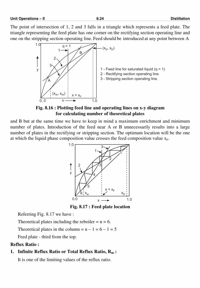
Unit Operations – II 8.24 Distillation
The point of intersection of 1, 2 and 3 falls in a triangle which represents a feed plate. The
triangle representing the feed plate has one corner on the rectifying section operating line and
one on the stripping section operating line. Feed should be introduced at any point between A
y
1.0
1.00, 0 x
q = 1
B1
2
3
A
(x , x )D D
x = xF(x , x )W W
1 - Feed line for saturated liquid (q = 1)
2 - Rectifying section operating line
3 - Stripping section operating line.
Fig. 8.16 : Plotting feed line and operating lines on x-y diagram
for calculating number of theoretical plates
and B but at the same time we have to keep in mind a maximum enrichment and minimum
number of plates. Introduction of the feed near A or B unnecessarily results into a large
number of plates in the rectifying or stripping section. The optimum location will be the one
at which the liquid phase composition value crosses the feed composition value xF.
y
x 1.0
1.0
4
3
2
5
xw xD6
0.0
x = xF
1
31
2
Fig. 8.17 : Feed plate location
Referring Fig. 8.17 we have :
Theoretical plates including the reboiler = n = 6.
Theoretical plates in the column = n – 1 = 6 – 1 = 5
Feed plate - third from the top.
Reflux Ratio :
1. Infinite Reflux Ratio or Total Reflux Ratio, R∞∞∞∞ :
It is one of the limiting values of the reflux ratio.
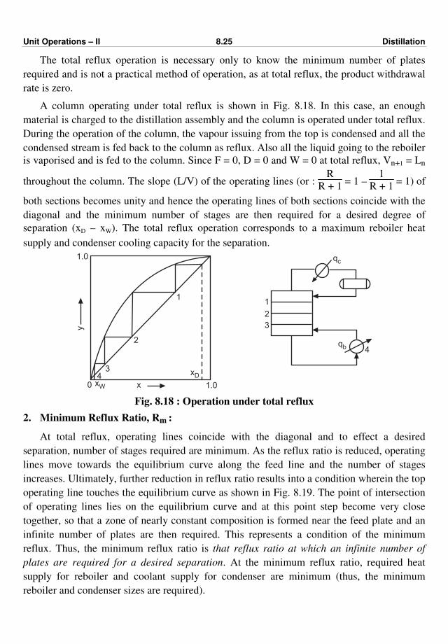
Unit Operations – II 8.25 Distillation
The total reflux operation is necessary only to know the minimum number of plates
required and is not a practical method of operation, as at total reflux, the product withdrawal
rate is zero.
A column operating under total reflux is shown in Fig. 8.18. In this case, an enough
material is charged to the distillation assembly and the column is operated under total reflux.
During the operation of the column, the vapour issuing from the top is condensed and all the
condensed stream is fed back to the column as reflux. Also all the liquid going to the reboiler
is vaporised and is fed to the column. Since F = 0, D = 0 and W = 0 at total reflux, Vn+1 = Ln
throughout the column. The slope (L/V) of the operating lines (or : R
R + 1 = 1 –
1
R + 1 = 1) of
both sections becomes unity and hence the operating lines of both sections coincide with the
diagonal and the minimum number of stages are then required for a desired degree of
separation (xD – xW). The total reflux operation corresponds to a maximum reboiler heat
supply and condenser cooling capacity for the separation.
x
y
4
1
2
3
1.0
0 xW
xD
1.0
1
2
3
4
qc
qb
Fig. 8.18 : Operation under total reflux
2. Minimum Reflux Ratio, Rm :
At total reflux, operating lines coincide with the diagonal and to effect a desired
separation, number of stages required are minimum. As the reflux ratio is reduced, operating
lines move towards the equilibrium curve along the feed line and the number of stages
increases. Ultimately, further reduction in reflux ratio results into a condition wherein the top
operating line touches the equilibrium curve as shown in Fig. 8.19. The point of intersection
of operating lines lies on the equilibrium curve and at this point step become very close
together, so that a zone of nearly constant composition is formed near the feed plate and an
infinite number of plates are then required. This represents a condition of the minimum
reflux. Thus, the minimum reflux ratio is that reflux ratio at which an infinite number of
plates are required for a desired separation. At the minimum reflux ratio, required heat
supply for reboiler and coolant supply for condenser are minimum (thus, the minimum
reboiler and condenser sizes are required).

Unit Operations – II 8.26 Distillation
1.0
y
x 1.00, 0
x = xF
Line - 1
Feed line
P
(x , )W xW
(x , )D xD
Line - 1operatingline for Rm
Fig. 8.19 : Minimum reflux ratio
Calculation of minimum reflux ratio (Rm) :
For liquid at its bubble point, the feed line is vertical (parallel to y-axis) and point 'C' lies
on the equilibrium curve and has the co-ordinates (xF, yF).
Draw the equilibrium curve and diagonal and draw the feed line, a vertical through the
point (xF, xF) on the diagonal. The point of intersection of the feed line with the equilibrium
curve is also a point of intersection of the operating lines at minimum reflux.
1.0
y
x 1.00, 0
P
C
A
yF
xF
xD
Fig. 8.20 : Method of obtaining Rm
Slope of the operating line AC, for the rectifying section, is given by
Rm
Rm + 1 =
xD – yF
xD – xF … (8.73)
Rm (xD – xF) = (Rm + 1) (xD – yF)
Rm · xD – Rm · xF = Rm xD – Rm yF + xD – yF
∴ Rm (yF – xF) = xD – yF
Rm = xD – yF
yF – xF … (8.74)
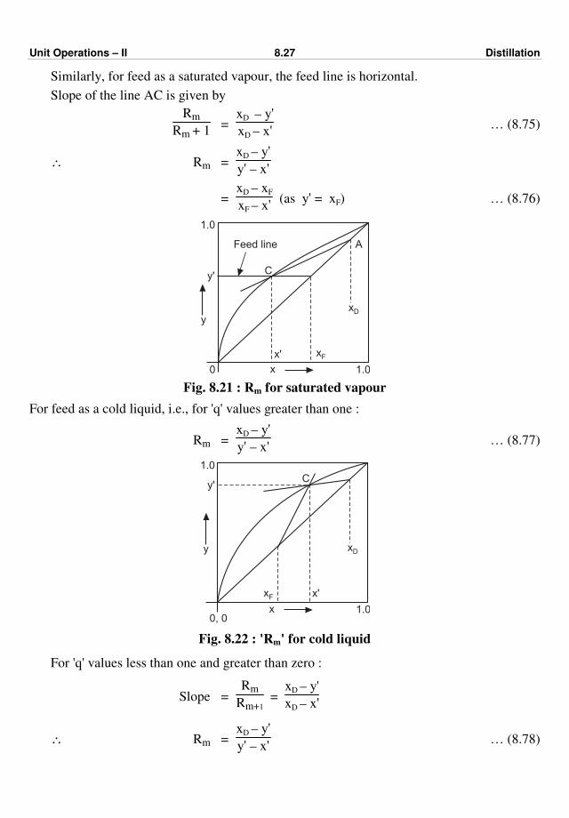
Unit Operations – II 8.27 Distillation
Similarly, for feed as a saturated vapour, the feed line is horizontal.
Slope of the line AC is given by
Rm
Rm + 1 =
xD – y'
xD – x' … (8.75)
∴ Rm = xD – y'
y' – x'
= xD – xF
xF – x' (as y' = xF) … (8.76)
y
y'
1.0
0 x
x' xF
1.0
Feed line
C
A
xD
Fig. 8.21 : Rm for saturated vapour
For feed as a cold liquid, i.e., for 'q' values greater than one :
Rm = xD – y'
y' – x' … (8.77)
y
1.0
0, 0x
x'xF
1.0
xD
y'C
Fig. 8.22 : 'Rm' for cold liquid
For 'q' values less than one and greater than zero :
Slope = Rm
Rm+1 =
xD – y'
xD – x'
∴ Rm = xD – y'
y' – x' … (8.78)

Unit Operations – II 8.28 Distillation
y
1.0
0, 0x
x' xF
1.0
xD
y'C
A
Fig. 8.23 : 'Rm' for feed-partially vapour
3. Optimum Reflux Ratio :
The optimum reflux ratio is defined as that reflux ratio at which the total cost of
operation (the sum of the fixed charges and the cost of heating and cooling) is minimum.
Any reflux ratio between infinite reflux ratio requiring a minimum number of plates and
minimum reflux ratio requiring an infinite number of plates is a workable system which
requires finite stages for a desired degree of separation. At minimum reflux ratio as infinite
number of plates are required, the fixed cost is also infinite while the cost of heat supply to
the reboiler and condenser coolant is minimum. As the reflux ratio is increased, the number
of plates decreases and the fixed cost decreases at first, passes through a minimum and then
increases as with a higher reflux ratio the diameter of the column and sizes of the reboiler
and condenser increases. The operating cost increases continuously with reflux ratio as it is
directly proportional to (R + 1). At total reflux, though the number of plates are minimum,
the cost of heat supply to reboiler and condenser coolant is maximum and also large capacity
RRm
Nm
N
Fig. 8.24 : Relation between reflux ratio and number of stages for distillation
reboiler and condenser are needed. The total cost which is the sum of the fixed cost and the
operating cost also decreases to a minimum and then increases with reflux ratio. The
optimum reflux ratio occurs at a point where the sum of the fixed cost and operating cost is
minimum. As a rough approximation, the optimum reflux ratio usually lies in the range of
1.1 to 1.5 times the minimum reflux ratio.
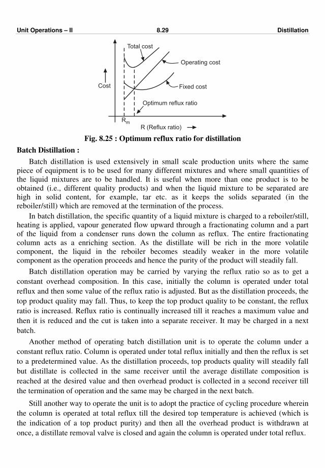
Unit Operations – II 8.29 Distillation
Cost
Total cost
Operating cost
Fixed cost
Optimum reflux ratio
R (Reflux ratio)
Rm
Fig. 8.25 : Optimum reflux ratio for distillation
Batch Distillation :
Batch distillation is used extensively in small scale production units where the same
piece of equipment is to be used for many different mixtures and where small quantities of
the liquid mixtures are to be handled. It is useful when more than one product is to be
obtained (i.e., different quality products) and when the liquid mixture to be separated are
high in solid content, for example, tar etc. as it keeps the solids separated (in the
reboiler/still) which are removed at the termination of the process.
In batch distillation, the specific quantity of a liquid mixture is charged to a reboiler/still,
heating is applied, vapour generated flow upward through a fractionating column and a part
of the liquid from a condenser runs down the column as reflux. The entire fractionating
column acts as a enriching section. As the distillate will be rich in the more volatile
component, the liquid in the reboiler becomes steadily weaker in the more volatile
component as the operation proceeds and hence the purity of the product will steadily fall.
Batch distillation operation may be carried by varying the reflux ratio so as to get a
constant overhead composition. In this case, initially the column is operated under total
reflux and then some value of the reflux ratio is adjusted. But as the distillation proceeds, the
top product quality may fall. Thus, to keep the top product quality to be constant, the reflux
ratio is increased. Reflux ratio is continually increased till it reaches a maximum value and
then it is reduced and the cut is taken into a separate receiver. It may be charged in a next
batch.
Another method of operating batch distillation unit is to operate the column under a
constant reflux ratio. Column is operated under total reflux initially and then the reflux is set
to a predetermined value. As the distillation proceeds, top products quality will steadily fall
but distillate is collected in the same receiver until the average distillate composition is
reached at the desired value and then overhead product is collected in a second receiver till
the termination of operation and the same may be charged in the next batch.
Still another way to operate the unit is to adopt the practice of cycling procedure wherein
the column is operated at total reflux till the desired top temperature is achieved (which is
the indication of a top product purity) and then all the overhead product is withdrawn at
once, a distillate removal valve is closed and again the column is operated under total reflux.

Unit Operations – II 8.30 Distillation
Vapour
Condenser
Accumulator
Distillate, D, xDReflux
Plate
Column
Vapour
Reboiler / Kettle
Steam
FeedF, xF
Condensate
Residue / Bottom product, W, xW
Column
Fig. 8.26 : Batch distillation unit
Azeotropes :
An azeotrope is a liquid mixture with an equilibrium vapour of the same composition as
the liquid. The dew point and bubble point are identical at azeotropic composition and the
mixture vaporises at a single temperature, so azeotropes are called constant boiling mixtures.
When an azeotrope is boiled, the vapour produced will have the same composition as the
liquid from which it is produced. Boiling of an ordinary solution takes place from the bubble
point to the dew point, whereas the boiling point of an azeotrope remains constant till the
entire liquid is vaporised. Close boiling components showing small deviations from ideality
may form an azeotrope. An azeotrope exhibits a maximum or a minimum boiling point
relative to the boiling points of pure liquids, thus are classified as maximum boiling and
minimum boiling azeotropes. The maximum boiling azeotrope occurs if the solution exhibits
negative deviation from ideality (Raoult's law) and the minimum boiling azeotrope occurs if
the solution exhibits positive deviation from ideality. Minimum boiling azeotrope will boil at
a temperature lower than the boiling points of pure components and maximum boiling
azeotrope will boil at higher temperature than the boiling points of the pure components. The
temperature–composition diagrams and equilibrium diagrams for liquid mixtures forming
azeotropes at constant pressure are shown in Fig. 8.27. Here we will see that the equilibrium
curve crosses the diagonal - which is an indication of the existence of an azeotrope, i.e., y = x
and the mixture will not be separated by ordinary distillation.
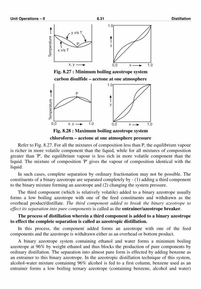
Unit Operations – II 8.31 Distillation
P
x v/s T
y v/s T
x, y
Tem
pera
ture
0,0 1.0
y
x
1.0
Fig. 8.27 : Minimum boiling azeotrope system
carbon disulfide – acetone at one atmosphere
0,0 1.0
y
x
1.0
P
x, y
Te
mp
era
ture
0,0 1.0
Fig. 8.28 : Maximum boiling azeotrope system
chloroform – acetone at one atmosphere pressure
Refer to Fig. 8.27. For all the mixtures of composition less than P, the equilibrium vapour
is richer in more volatile component than the liquid, while for all mixtures of composition
greater than 'P', the equilibrium vapour is less rich in more volatile component than the
liquid. The mixture of composition 'P' gives the vapour of composition identical with the
liquid.
In such cases, complete separation by ordinary fractionation may not be possible. The
constituents of a binary azeotrope are separated completely by - (1) adding a third component
to the binary mixture forming an azeotrope and (2) changing the system pressure.
The third component (which is relatively volatile) added to a binary azeotrope usually
forms a low boiling azeotrope with one of the feed constituents and withdrawn as the
overhead product/distillate. The third component added to break the binary azeotrope to
effect its separation into pure components is called as the entrainer/azeotrope breaker.
The process of distillation wherein a third component is added to a binary azeotrope
to effect the complete separation is called as azeotropic distillation.
In this process, the component added forms an azeotrope with one of the feed
components and the azeotrope is withdrawn either as an overhead or bottom product.
A binary azeotrope system containing ethanol and water forms a minimum boiling
azeotrope at 96% by weight ethanol and thus blocks the production of pure components by
ordinary distillation. The separation into almost pure form is effected by adding benzene as
an entrainer to this binary azeotrope. In the azeotropic distillation technique of this system,
alcohol-water mixture containing 96% alcohol is fed to a first column, benzene used as an
entrainer forms a low boiling ternary azeotrope (containing benzene, alcohol and water)
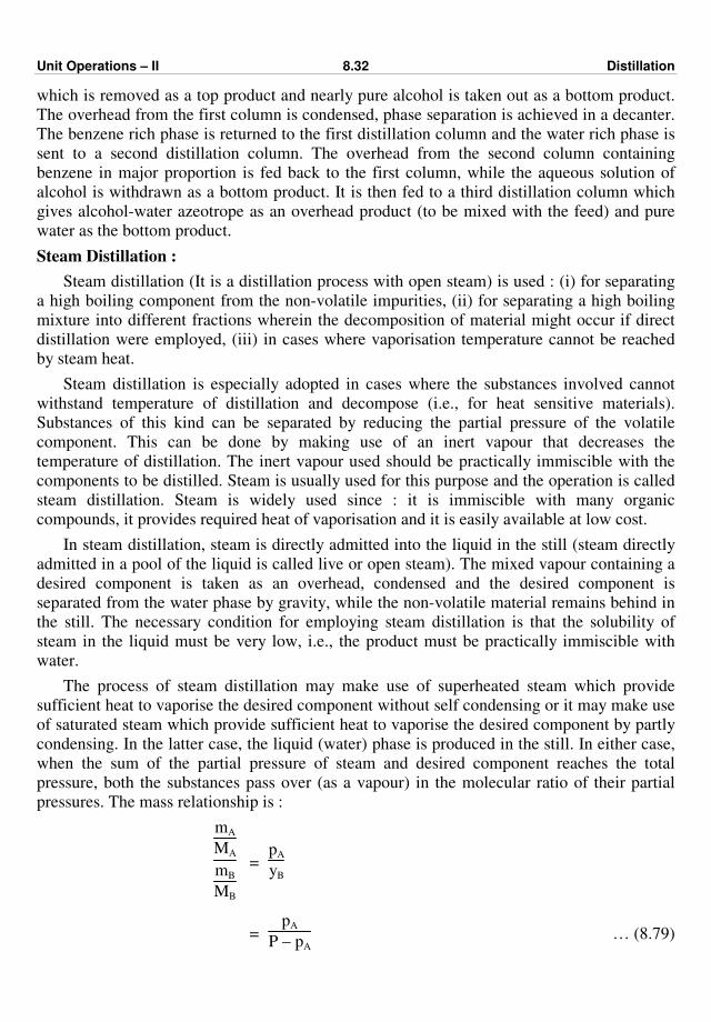
Unit Operations – II 8.32 Distillation
which is removed as a top product and nearly pure alcohol is taken out as a bottom product.
The overhead from the first column is condensed, phase separation is achieved in a decanter.
The benzene rich phase is returned to the first distillation column and the water rich phase is
sent to a second distillation column. The overhead from the second column containing
benzene in major proportion is fed back to the first column, while the aqueous solution of
alcohol is withdrawn as a bottom product. It is then fed to a third distillation column which
gives alcohol-water azeotrope as an overhead product (to be mixed with the feed) and pure
water as the bottom product.
Steam Distillation :
Steam distillation (It is a distillation process with open steam) is used : (i) for separating
a high boiling component from the non-volatile impurities, (ii) for separating a high boiling
mixture into different fractions wherein the decomposition of material might occur if direct
distillation were employed, (iii) in cases where vaporisation temperature cannot be reached
by steam heat.
Steam distillation is especially adopted in cases where the substances involved cannot
withstand temperature of distillation and decompose (i.e., for heat sensitive materials).
Substances of this kind can be separated by reducing the partial pressure of the volatile
component. This can be done by making use of an inert vapour that decreases the
temperature of distillation. The inert vapour used should be practically immiscible with the
components to be distilled. Steam is usually used for this purpose and the operation is called
steam distillation. Steam is widely used since : it is immiscible with many organic
compounds, it provides required heat of vaporisation and it is easily available at low cost.
In steam distillation, steam is directly admitted into the liquid in the still (steam directly
admitted in a pool of the liquid is called live or open steam). The mixed vapour containing a
desired component is taken as an overhead, condensed and the desired component is
separated from the water phase by gravity, while the non-volatile material remains behind in
the still. The necessary condition for employing steam distillation is that the solubility of
steam in the liquid must be very low, i.e., the product must be practically immiscible with
water.
The process of steam distillation may make use of superheated steam which provide
sufficient heat to vaporise the desired component without self condensing or it may make use
of saturated steam which provide sufficient heat to vaporise the desired component by partly
condensing. In the latter case, the liquid (water) phase is produced in the still. In either case,
when the sum of the partial pressure of steam and desired component reaches the total
pressure, both the substances pass over (as a vapour) in the molecular ratio of their partial
pressures. The mass relationship is :
mA
MA
mB
MB
= pA
yB
= pA
P – pA … (8.79)
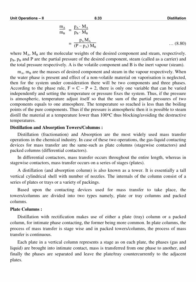
Unit Operations – II 8.33 Distillation
mA
mB =
pA · MA
pB · MB
= pA MA
(P – pA) MB … (8.80)
where MA, MB are the molecular weights of the desired component and steam, respectively.
pB, pB and P are the partial pressure of the desired component, steam (called as a carrier) and
the total pressure respectively. A is the volatile component and B is the inert vapour (steam).
mA, mB are the masses of desired component and steam in the vapour respectively. When
the water phase is present and effect of a non-volatile material on vaporisation is neglected,
then for the system under consideration there will be two components and three phases.
According to the phase rule, F = C – P + 2, there is only one variable that can be varied
independently and setting the temperature or pressure fixes the system. Thus, if the pressure
is atmospheric, temperature adjust itself so that the sum of the partial pressures of two
components equals to one atmosphere. The temperature so reached is less than the boiling
points of the pure components. Thus if the pressure is atmospheric then it is possible to steam
distill the material at a temperature lower than 100oC thus blocking/avoiding the destructive
temperatures.
Distillation and Absorption Towers/Columns :
Distillation (fractionation) and Absorption are the most widely used mass transfer
operations in the chemical industry. In case of these two operations, the gas-liquid contacting
devices for mass transfer are the same-such as plate columns (stagewise contactors) and
packed columns (differential contactors).
In differential contactors, mass transfer occurs throughout the entire length, whereas in
stagewise contactors, mass transfer occurs on a series of stages (plates).
A distillation (and absorption column) is also known as a tower. It is essentially a tall
vertical cylindrical shell with number of nozzles. The internals of the column consist of a
series of plates or trays or a variety of packings.
Based upon the contacting devices used for mass transfer to take place, the
towers/columns are divided into two types namely, plate or tray columns and packed
columns.
Plate Columns :
Distillation with rectification makes use of either a plate (tray) column or a packed
column, for intimate phase contacting, the former being more common. In plate columns, the
process of mass transfer is stage wise and in packed towers/columns, the process of mass
transfer is continuous.
Each plate in a vertical column represents a stage as on each plate, the phases (gas and
liquid) are brought into intimate contact, mass is transferred from one phase to another, and
finally the phases are separated and leave the plate/tray countercurrently to the adjacent
plates.
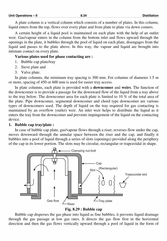
Unit Operations – II 8.34 Distillation
A plate column is a vertical column which consists of a number of plates. In this column,
liquid enters from the top, flows over every plate and from plate to plate via down comers.
A certain height of a liquid pool is maintained on each plate with the help of an outlet
weir. Gas/vapour enters in the column from the bottom inlet and flows upward through the
openings in the plate, it bubbles through the pool of liquid on each plate, disengages from the
liquid and passes to the plate above. In this way, the vapour and liquid are brought into
intimate contact on every plate.
Various plates used for phase contacting are :
1. Bubble cap plate/tray
2. Sieve plate and
3. Valve plate.
In plate columns, the minimum tray spacing is 300 mm. For columns of diameter 1.5 m
or more, spacing of 450 or 600 mm is used for easier tray access.
In plate columns, each plate is provided with a downcomer and weirs. The function of
the downcomer is to provide a passage for the downward flow of the liquid from a tray above
to the tray below. The downcomer area for each plate is limited to 10 % of the total area of
the plate. Pipe downcomer, segmental downcomer and chord type downcomer are various
types of downcomers used. The depth of liquid on the tray required for gas contacting is
maintained by an overflow (outlet) weir. An inlet weir helps to distribute the liquid as it
enters the tray from the downcomer and prevents impingement of the liquid on the contacting
device.
1. Bubble cap tray/plate :
In case of bubble cap plate, gas/vapour flows through a riser, reverses flow under the cap,
moves downward through the annular space between the riser and the cap, and finally it
bubbles into a pool of liquid through a series of slots (openings) provided along the periphery
of the cap in its lower portion. The slots may be circular, rectangular or trapezoidal in shape.
RiserTray plate
Slot
Cap
(Rectangular)
Clamping nut-bolt
Gas flow
Trapezoidal slot
Fig. 8.29 : Bubble cap
Bubble cap disperses the gas phase into liquid as fine bubbles, it prevents liquid drainage
through the gas passage at low gas rates. It directs the gas flow first in the horizontal
direction and then the gas flows vertically upward through a pool of liquid in the form of
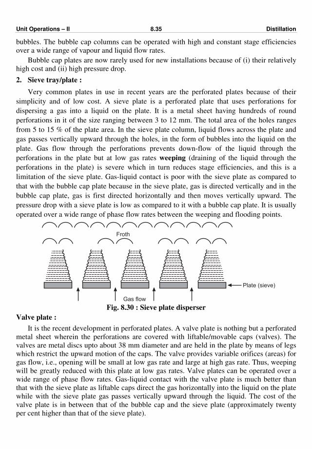
Unit Operations – II 8.35 Distillation
bubbles. The bubble cap columns can be operated with high and constant stage efficiencies
over a wide range of vapour and liquid flow rates.
Bubble cap plates are now rarely used for new installations because of (i) their relatively
high cost and (ii) high pressure drop.
2. Sieve tray/plate :
Very common plates in use in recent years are the perforated plates because of their
simplicity and of low cost. A sieve plate is a perforated plate that uses perforations for
dispersing a gas into a liquid on the plate. It is a metal sheet having hundreds of round
perforations in it of the size ranging between 3 to 12 mm. The total area of the holes ranges
from 5 to 15 % of the plate area. In the sieve plate column, liquid flows across the plate and
gas passes vertically upward through the holes, in the form of bubbles into the liquid on the
plate. Gas flow through the perforations prevents down-flow of the liquid through the
perforations in the plate but at low gas rates weeping (draining of the liquid through the
perforations in the plate) is severe which in turn reduces stage efficiencies, and this is a
limitation of the sieve plate. Gas-liquid contact is poor with the sieve plate as compared to
that with the bubble cap plate because in the sieve plate, gas is directed vertically and in the
bubble cap plate, gas is first directed horizontally and then moves vertically upward. The
pressure drop with a sieve plate is low as compared to it with a bubble cap plate. It is usually
operated over a wide range of phase flow rates between the weeping and flooding points.
Froth
Gas flow
Plate (sieve)
Fig. 8.30 : Sieve plate disperser
Valve plate :
It is the recent development in perforated plates. A valve plate is nothing but a perforated
metal sheet wherein the perforations are covered with liftable/movable caps (valves). The
valves are metal discs upto about 38 mm diameter and are held in the plate by means of legs
which restrict the upward motion of the caps. The valve provides variable orifices (areas) for
gas flow, i.e., opening will be small at low gas rate and large at high gas rate. Thus, weeping
will be greatly reduced with this plate at low gas rates. Valve plates can be operated over a
wide range of phase flow rates. Gas-liquid contact with the valve plate is much better than
that with the sieve plate as liftable caps direct the gas horizontally into the liquid on the plate
while with the sieve plate gas passes vertically upward through the liquid. The cost of the
valve plate is in between that of the bubble cap and the sieve plate (approximately twenty
per cent higher than that of the sieve plate).
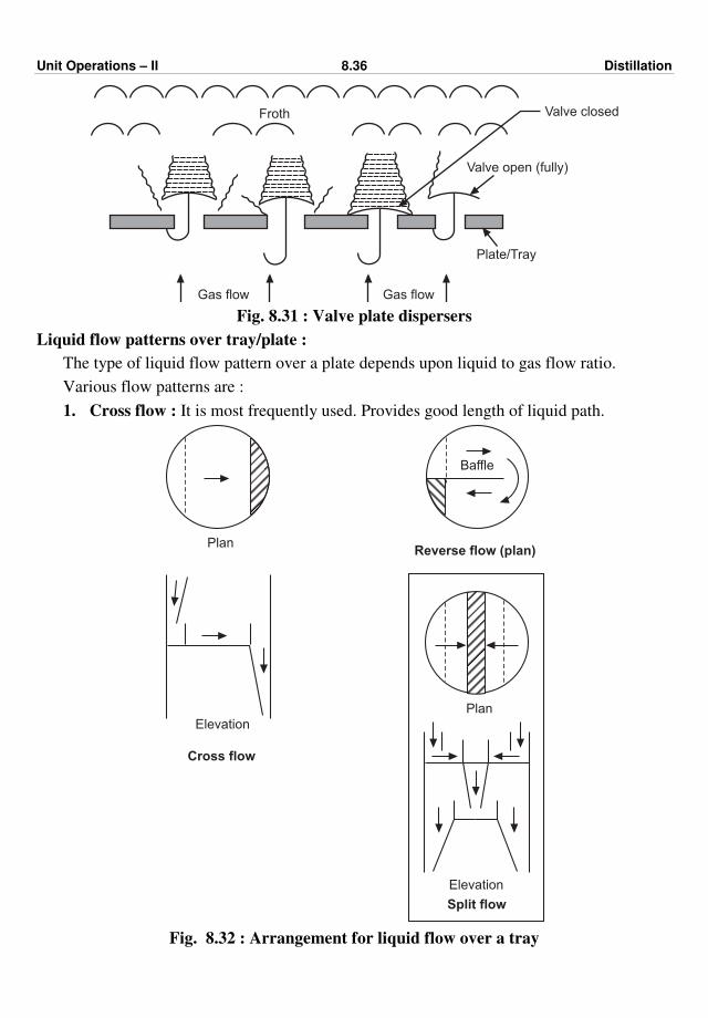
Unit Operations – II 8.36 Distillation
Plate/Tray
Valve open (fully)
Valve closedFroth
Gas flow Gas flow Fig. 8.31 : Valve plate dispersers
Liquid flow patterns over tray/plate :
The type of liquid flow pattern over a plate depends upon liquid to gas flow ratio.
Various flow patterns are :
1. Cross flow : It is most frequently used. Provides good length of liquid path.
Baffle
PlanReverse flow (plan)
Elevation
Cross flow
Split flow
Elevation
Plan
Fig. 8.32 : Arrangement for liquid flow over a tray
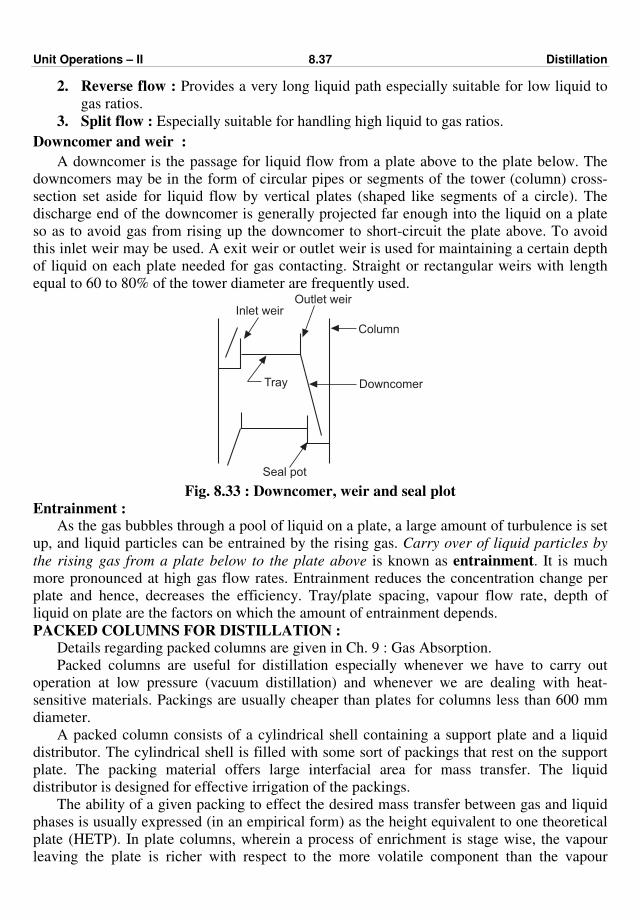
Unit Operations – II 8.37 Distillation
2. Reverse flow : Provides a very long liquid path especially suitable for low liquid to
gas ratios.
3. Split flow : Especially suitable for handling high liquid to gas ratios.
Downcomer and weir :
A downcomer is the passage for liquid flow from a plate above to the plate below. The
downcomers may be in the form of circular pipes or segments of the tower (column) cross-
section set aside for liquid flow by vertical plates (shaped like segments of a circle). The
discharge end of the downcomer is generally projected far enough into the liquid on a plate
so as to avoid gas from rising up the downcomer to short-circuit the plate above. To avoid
this inlet weir may be used. A exit weir or outlet weir is used for maintaining a certain depth
of liquid on each plate needed for gas contacting. Straight or rectangular weirs with length
equal to 60 to 80% of the tower diameter are frequently used.
Seal pot
Inlet weirOutlet weir
Column
DowncomerTray
Fig. 8.33 : Downcomer, weir and seal plot
Entrainment : As the gas bubbles through a pool of liquid on a plate, a large amount of turbulence is set
up, and liquid particles can be entrained by the rising gas. Carry over of liquid particles by
the rising gas from a plate below to the plate above is known as entrainment. It is much
more pronounced at high gas flow rates. Entrainment reduces the concentration change per
plate and hence, decreases the efficiency. Tray/plate spacing, vapour flow rate, depth of
liquid on plate are the factors on which the amount of entrainment depends.
PACKED COLUMNS FOR DISTILLATION : Details regarding packed columns are given in Ch. 9 : Gas Absorption.
Packed columns are useful for distillation especially whenever we have to carry out
operation at low pressure (vacuum distillation) and whenever we are dealing with heat-
sensitive materials. Packings are usually cheaper than plates for columns less than 600 mm
diameter.
A packed column consists of a cylindrical shell containing a support plate and a liquid
distributor. The cylindrical shell is filled with some sort of packings that rest on the support
plate. The packing material offers large interfacial area for mass transfer. The liquid
distributor is designed for effective irrigation of the packings.
The ability of a given packing to effect the desired mass transfer between gas and liquid
phases is usually expressed (in an empirical form) as the height equivalent to one theoretical
plate (HETP). In plate columns, wherein a process of enrichment is stage wise, the vapour
leaving the plate is richer with respect to the more volatile component than the vapour
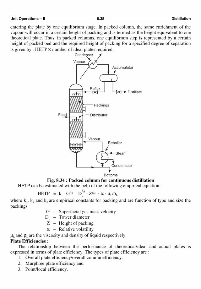
Unit Operations – II 8.38 Distillation
entering the plate by one equilibrium stage. In packed column, the same enrichment of the
vapour will occur in a certain height of packing and is termed as the height equivalent to one
theoretical plate. Thus, in packed columns, one equilibrium step is represented by a certain
height of packed bed and the required height of packing for a specified degree of separation
is given by : HETP × number of ideal plates required.
Packings
DistributorFeed
RefluxDistillate
Accumulator
Condenser
Steam
Reboiler
Bottoms
Vapour
Vapour
Condensate
Fig. 8.34 : Packed column for continuous distillation
HETP can be estimated with the help of the following empirical equation :
HETP = k1 · Gk2 · D
k3
t · Z1/3 · α · µL/ρL
where k1, k2 and k3 are empirical constants for packing and are function of type and size the
packings
G – Superfacial gas mass velocity
Dt – Tower diameter
Z – Height of packing
α – Relative volatility
µL and ρL are the viscosity and density of liquid respectively.
Plate Efficiencies : The relationship between the performance of theoretical/ideal and actual plates is
expressed in terms of plate efficiency. The types of plate efficiency are :
1. Overall plate efficiency/overall column efficiency.
2. Murphree plate efficiency and
3. Point/local efficiency.

Unit Operations – II 8.39 Distillation
Overall plate efficiency is the ratio of the number of ideal or theoretical plates (stages)
required to produce a given separation in the entire column to the number of actual plates
required to effect the same separation.
If the overall efficiency is 60% and 12 ideal plates are called for, then the actual plates
needed are 12/0.60 = 20
Murphree plate efficiency :
It applies to a individual plate in a column and is defined as the actual change in average
composition accomplished by a given plate divided by the change in average composition if
the vapour leaving the plate were in equilibrium with the liquid leaving the plate.
Point efficiency is defined in the same manner as the murphree plate efficiency but it
applies to a single location on a given plate.
SOLVED EXAMPLES
Example 8.1 : A mixture of benzene and toluene boils at 368 K (95o C) under a pressure
of 101.325 kPa. Determine the composition of the boiling liquid assuming that mixture obeys
Raoult's law.
At 368 K (95o C), the vapour pressure of benzene is 155.56 kPa and that of toluene is
63.98 kPa.
Solution : Let xA be the mole fraction of benzene in the liquid mixture.
We know that : xA = P – p
oB
poA – p
oB
where P = 101.325 kPa
poB = 63.98 kPa
poA = 155.56 kPa
xA = 101.325 – 63.98
155.56 – 63.98 = 0.408
Mole % of benzene in
the boiling liquid = 0.408 × 100 = 40.8 … Ans.
Example 8.2 : Calculate the equilibrium compositions of the liquid and the vapour
phases for a mixture of methyl alcohol and water at a temperature of 323 K (50o C) and
under a pressure of 40 kPa. Assume that both the liquid and vapour behave ideally.
Data : V.P. of methanol at 323 K (50o C) = 53.32 kPa
V.P. of water at 323 K (50o C) = 12.33 kPa.
Solution : Let xA and yA be the mole fraction of methyl alcohol in the liquid and vapour.
The partial pressure of methyl alcohol in the vapour phase is given by
pA = poA xA = 53.32 xA
Similarly, pB = partial pressure of water
= poB xB = 12.33 (1 – xA)
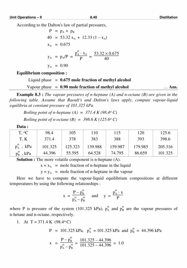
Unit Operations – II 8.40 Distillation
According to the Dalton's law of partial pressures,
P = pA + pB
40 = 53.32 xA + 12.33 (1 – xA)
xA = 0.675
yA = pA/P = p
oA · xA
P =
53.32 × 0.675
40
yA = 0.90
Equilibrium composition :
Liquid phase = 0.675 mole fraction of methyl alcohol
Vapour phase = 0.90 mole fraction of methyl alcohol … Ans.
Example 8.3 : The vapour pressures of n-heptane (A) and n-octane (B) are given in the
following table. Assume that Raoult's and Dalton's laws apply, compute vapour-liquid
equilibria at constant pressure of 101.325 kPa
Boiling point of n-heptane (A) = 371.4 K (98.4o C)
Boiling point of n-octane (B) = 398.6 K (125.6o C)
Data :
T, oC
T, K
poA , kPa
poB , kPa
98.4
371.4
101.325
44.396
105
378
125.323
55.595
110
383
139.988
64.528
115
388
159.987
74.795
120
393
179.985
86.659
125.6
398.6
205.316
101.325
Solution : The more volatile component is n-heptane (A).
x = xA = mole fraction of n-heptane in the liquid
y = yA = mole fraction of n-heptane in the vapour
Here we have to compute the vapour-liquid equilibrium compositions at different
temperatures by using the following relationships :
x = P – p
oB
poA – p
oB
and y = p
oA · x
P
where P is pressure of the system (101.325 kPa), poA and p
oB are the vapour pressures of
n-hetane and n-octane, respectively.
1. At T = 371.4 K (98.4o C)
P = 101.325 kPa, poA = 101.325 kPa and p
oB = 44.396 kPa
x = P – p
oB
poA – p
oB
= 101.325 – 44.396
101.325 – 44.396 = 1.0
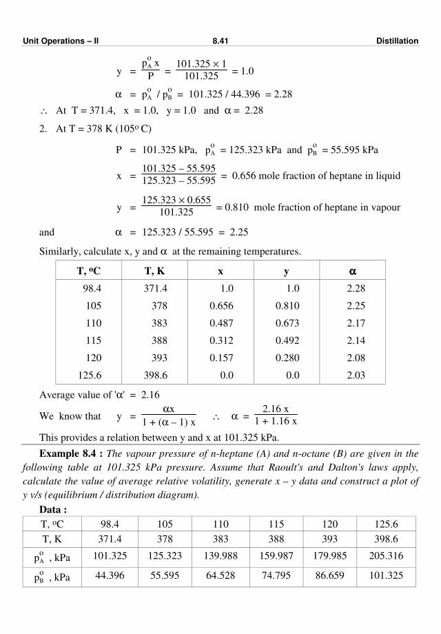
Unit Operations – II 8.41 Distillation
y = p
oA x
P =
101.325 × 1
101.325 = 1.0
α = poA / p
oB = 101.325 / 44.396 = 2.28
∴ At T = 371.4, x = 1.0, y = 1.0 and α = 2.28
2. At T = 378 K (105o C)
P = 101.325 kPa, poA = 125.323 kPa and p
oB = 55.595 kPa
x = 101.325 – 55.595
125.323 – 55.595 = 0.656 mole fraction of heptane in liquid
y = 125.323 × 0.655
101.325 = 0.810 mole fraction of heptane in vapour
and α = 125.323 / 55.595 = 2.25
Similarly, calculate x, y and α at the remaining temperatures.
T, oC T, K x y αααα
98.4
105
110
115
120
125.6
371.4
378
383
388
393
398.6
1.0
0.656
0.487
0.312
0.157
0.0
1.0
0.810
0.673
0.492
0.280
0.0
2.28
2.25
2.17
2.14
2.08
2.03
Average value of 'α' = 2.16
We know that y = αx
1 + (α – 1) x ∴ α =
2.16 x
1 + 1.16 x
This provides a relation between y and x at 101.325 kPa.
Example 8.4 : The vapour pressure of n-heptane (A) and n-octane (B) are given in the
following table at 101.325 kPa pressure. Assume that Raoult's and Dalton's laws apply,
calculate the value of average relative volatility, generate x – y data and construct a plot of
y v/s (equilibrium / distribution diagram).
Data :
T, oC 98.4 105 110 115 120 125.6
T, K 371.4 378 383 388 393 398.6
poA , kPa 101.325 125.323 139.988 159.987 179.985 205.316
poB , kPa 44.396 55.595 64.528 74.795 86.659 101.325
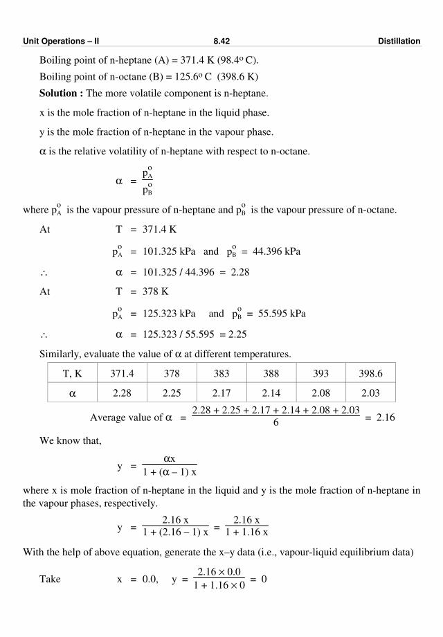
Unit Operations – II 8.42 Distillation
Boiling point of n-heptane (A) = 371.4 K (98.4o C).
Boiling point of n-octane (B) = 125.6o C (398.6 K)
Solution : The more volatile component is n-heptane.
x is the mole fraction of n-heptane in the liquid phase.
y is the mole fraction of n-heptane in the vapour phase.
α is the relative volatility of n-heptane with respect to n-octane.
α = p
oA
poB
where poA is the vapour pressure of n-heptane and p
oB is the vapour pressure of n-octane.
At T = 371.4 K
poA = 101.325 kPa and p
oB = 44.396 kPa
∴ α = 101.325 / 44.396 = 2.28
At T = 378 K
poA = 125.323 kPa and p
oB = 55.595 kPa
∴ α = 125.323 / 55.595 = 2.25
Similarly, evaluate the value of α at different temperatures.
T, K 371.4 378 383 388 393 398.6
α 2.28 2.25 2.17 2.14 2.08 2.03
Average value of α = 2.28 + 2.25 + 2.17 + 2.14 + 2.08 + 2.03
6 = 2.16
We know that,
y = αx
1 + (α – 1) x
where x is mole fraction of n-heptane in the liquid and y is the mole fraction of n-heptane in
the vapour phases, respectively.
y = 2.16 x
1 + (2.16 – 1) x =
2.16 x
1 + 1.16 x
With the help of above equation, generate the x–y data (i.e., vapour-liquid equilibrium data)
Take x = 0.0, y = 2.16 × 0.0
1 + 1.16 × 0 = 0

Unit Operations – II 8.43 Distillation
Take x = 0.10
y = 2.16 × 0.10
1 + 1.16 × 0.1 = 0.193 ≈ 0.19
Take x = 0.20
y = 2.16 × 0.20
1 + 1.16 × 0.20 = 0.351
Similarly, take x = 0.30, 0.40, 0.50 … 1.0 and evaluate corresponding values of y.
x 0 0.10 0.20 0.30 0.40 0.50 0.60 0.70 0.8 0.90 1.0
y 0 0.19 0.35 0.48 0.59 0.68 0.76 0.83 0.90 0.95 1.0
The x-y diagram is shown in Fig. Ex. 8.4.
0.1 0.2 0.3 0.4 0.5 0.6 0.7 0.8 0.9 1.0
x
0,0
0.1
0.2
0.3
0.4
0.5
0.6
0.7
0.8
0.9
1.0
y v/s x
y = x
y
Fig. Ex 8.4
Example 8.5 : For the system n-heptane and n-octane given in exercise 8.3, construct
T-x and T-y plots.
Solution : Boiling point of n-heptane (A) = 371.4 K (98.4o C)
Boiling point of n-octane (B) = 398.6 K (125.6o C)
On the ordinate through x = 0, y = 0, mark the boiling point of n-octane (398.6 K)
On the ordinate through x = 1, y = 1, mark the boiling point of n-heptane (371.4 K)
The T-x and T-y plots are shown in Fig. Ex 8.5.
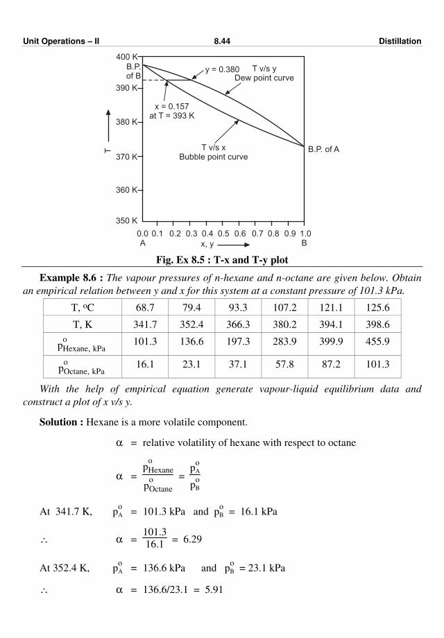
Unit Operations – II 8.44 Distillation
T
x, yA B
400 K
B.P.of B
390 K
380 K
370 K
360 K
350 K
0.0 0.1 0.2 0.3 0.4 0.5 0.6 0.7 0.8 0.9 1.0
B.P. of AT v/s xBubble point curve
x = 0.157at T = 393 K
y = 0.380 T v/s yDew point curve
Fig. Ex 8.5 : T-x and T-y plot
Example 8.6 : The vapour pressures of n-hexane and n-octane are given below. Obtain
an empirical relation between y and x for this system at a constant pressure of 101.3 kPa.
T, oC 68.7 79.4 93.3 107.2 121.1 125.6
T, K 341.7 352.4 366.3 380.2 394.1 398.6
po
Hexane‚ kPa 101.3 136.6 197.3 283.9 399.9 455.9
po
Octane‚ kPa 16.1 23.1 37.1 57.8 87.2 101.3
With the help of empirical equation generate vapour-liquid equilibrium data and
construct a plot of x v/s y.
Solution : Hexane is a more volatile component.
α = relative volatility of hexane with respect to octane
α = p
o
Hexane
po
Octane
= p
oA
poB
At 341.7 K, poA = 101.3 kPa and p
oB = 16.1 kPa
∴ α = 101.3
16.1 = 6.29
At 352.4 K, poA = 136.6 kPa and p
oB = 23.1 kPa
∴ α = 136.6/23.1 = 5.91
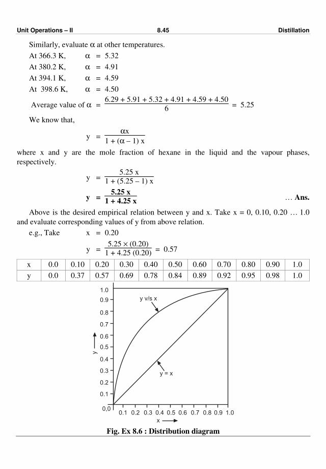
Unit Operations – II 8.45 Distillation
Similarly, evaluate α at other temperatures.
At 366.3 K, α = 5.32
At 380.2 K, α = 4.91
At 394.1 K, α = 4.59
At 398.6 K, α = 4.50
Average value of α = 6.29 + 5.91 + 5.32 + 4.91 + 4.59 + 4.50
6 = 5.25
We know that,
y = αx
1 + (α – 1) x
where x and y are the mole fraction of hexane in the liquid and the vapour phases,
respectively.
y = 5.25 x
1 + (5.25 – 1) x
y = 5.25 x
1 + 4.25 x … Ans.
Above is the desired empirical relation between y and x. Take x = 0, 0.10, 0.20 … 1.0
and evaluate corresponding values of y from above relation.
e.g., Take x = 0.20
y = 5.25 × (0.20)
1 + 4.25 (0.20) = 0.57
x 0.0 0.10 0.20 0.30 0.40 0.50 0.60 0.70 0.80 0.90 1.0
y 0.0 0.37 0.57 0.69 0.78 0.84 0.89 0.92 0.95 0.98 1.0
y v/s x
1.0
0.9
0.8
0.7
0.6
0.5
0.4
0.3
0.2
0.1
1.00.90.80.70.60.50.40.30.20.10,0
y
y = x
x
Fig. Ex 8.6 : Distribution diagram
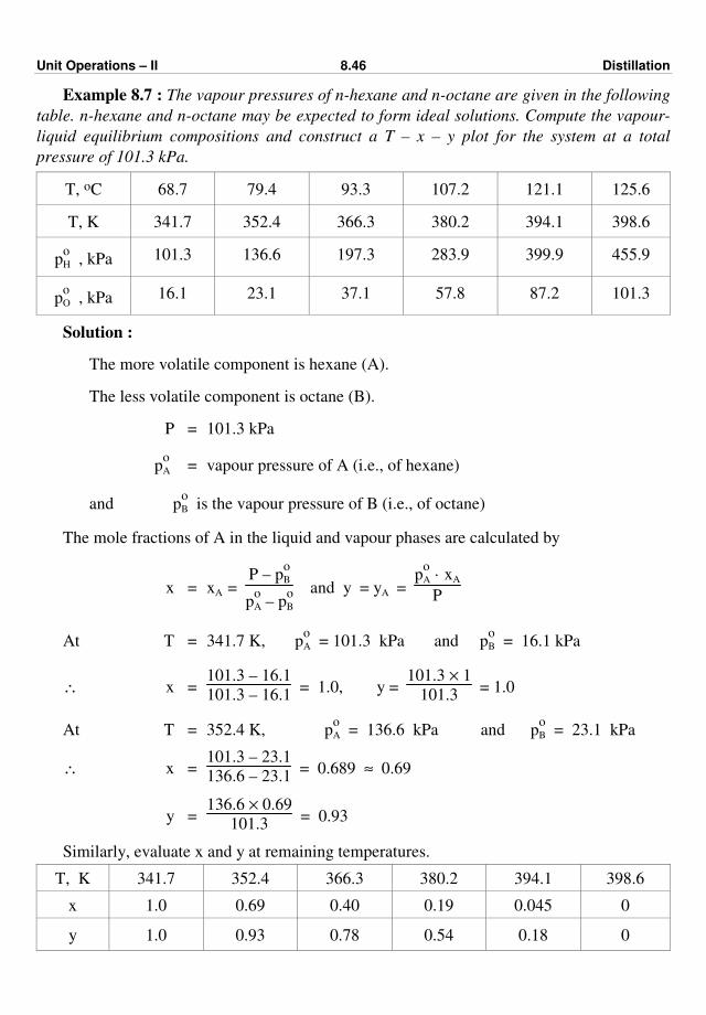
Unit Operations – II 8.46 Distillation
Example 8.7 : The vapour pressures of n-hexane and n-octane are given in the following
table. n-hexane and n-octane may be expected to form ideal solutions. Compute the vapour-
liquid equilibrium compositions and construct a T – x – y plot for the system at a total
pressure of 101.3 kPa.
T, oC 68.7 79.4 93.3 107.2 121.1 125.6
T, K 341.7 352.4 366.3 380.2 394.1 398.6
poH , kPa 101.3 136.6 197.3 283.9 399.9 455.9
poO , kPa 16.1 23.1 37.1 57.8 87.2 101.3
Solution :
The more volatile component is hexane (A).
The less volatile component is octane (B).
P = 101.3 kPa
poA = vapour pressure of A (i.e., of hexane)
and poB is the vapour pressure of B (i.e., of octane)
The mole fractions of A in the liquid and vapour phases are calculated by
x = xA = P – p
oB
poA – p
oB
and y = yA = p
oA · xA
P
At T = 341.7 K, poA = 101.3 kPa and p
oB = 16.1 kPa
∴ x = 101.3 – 16.1
101.3 – 16.1 = 1.0, y =
101.3 × 1
101.3 = 1.0
At T = 352.4 K, poA = 136.6 kPa and p
oB = 23.1 kPa
∴ x = 101.3 – 23.1
136.6 – 23.1 = 0.689 ≈ 0.69
y = 136.6 × 0.69
101.3 = 0.93
Similarly, evaluate x and y at remaining temperatures.
T, K 341.7 352.4 366.3 380.2 394.1 398.6
x 1.0 0.69 0.40 0.19 0.045 0
y 1.0 0.93 0.78 0.54 0.18 0
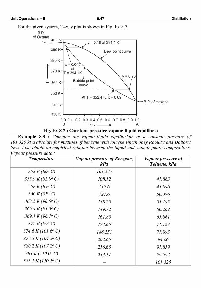
Unit Operations – II 8.47 Distillation
For the given system, T–x, y plot is shown in Fig. Ex 8.7.
T
x, y AB
400 K
B.P.of Octane
390 K
380 K
370 K
360 K
330 K
0.0 0.1 0.2 0.3 0.4 0.5 0.6 0.7 0.8 0.9 1.0
Bubble pointcurve
x = 0.045at
T = 394.1K
y = 0.18 at 394.1 K
Dew point curve
y = 0.93
350 K
340 K
At T = 352.4 K, x = 0.69
B.P. of Hexane
Fig. Ex 8.7 : Constant-pressure vapour-liquid equilibria
Example 8.8 : Compute the vapour-liquid equilibrium at a constant pressure of
101.325 kPa absolute for mixtures of benzene with toluene which obey Raoult's and Dalton's
laws. Also obtain an empirical relation between the liquid and vapour phase compositions.
Vapour pressure data :
Temperature Vapour pressure of Benzene, kPa
Vapour pressure of Toluene, kPa
353 K (80o C)
355.9 K (82.9o C)
358 K (85o C)
360 K (87o C)
363.5 K (90.5o C)
366.4 K (93.3o C)
369.1 K (96.1o C)
372 K (99o C)
374.6 K (101.6o C)
377.5 K (104.5o C)
380.2 K (107.2o C)
383 K (110.0o C)
383.1 K (110.1o C)
101.325
108.12
117.6
127.6
138.25
149.72
161.85
174.65
188.251
202.65
216.65
234.11
–
–
41.863
45.996
50.396
55.195
60.262
65.861
71.727
77.993
84.66
91.859
99.592
101.325

Unit Operations – II 8.48 Distillation
Solution : In the benzene – toluene mixture, the boiling point of pure benzene (A) is
353 K (80o C) and that of pure toluene (B) is 383.1 K (110.1o C). Thus, benzene is a more
volatile component. Let poA, p
oB and P be the vapour pressure of benzene, toluene and
constant total pressure. Let x and y be the equilibrium liquid phase and vapour phase
compositions.
i.e., x – mole fraction of benzene (more volatile component) in the liquid phase
y – mole fraction of benzene (more volatile component) in the vapour phase.
x and y can be calculated by using the following relations :
x = P – p
oB
poA – p
oB
and y = p
oA · x
P
P = 101.325 kPa
With the help of above two relations find x and y at each given temperature in the data.
For example,
1. At T = 358 K (85o C)
poA = 117.6 kPa and p
oB = 45.996 kPa
Therefore, x = P – p
oB
poA – p
oB
x = 101.325 – 45.996
117.6 – 45.996 = 0.773
and y = p
oA · x
P =
117.6 (0.773)
101.325 = 0.897
2. At T = 355.9 K
poA = 108.12 kPa
and poB = 41.863 kPa
x = 101.325 – 41.863
108.12 – 41.863 = 0.897
and y = 108.12 × 0.897
101.325 = 0.958
3. At T = 353 K
pA = 101.325 kPa
x = P – p
oB
poA – p
oB
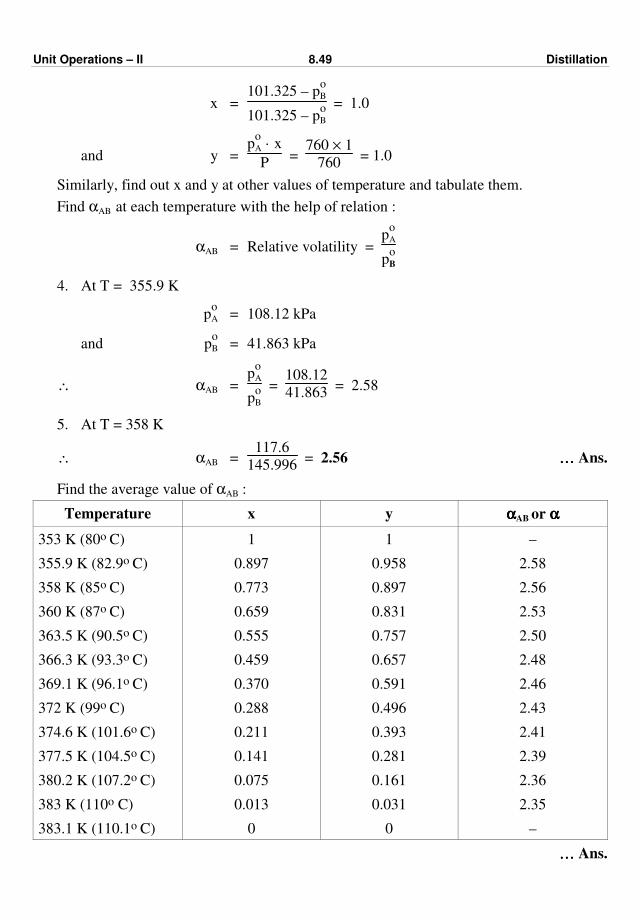
Unit Operations – II 8.49 Distillation
x = 101.325 – p
oB
101.325 – poB
= 1.0
and y = p
oA · x
P =
760 × 1
760 = 1.0
Similarly, find out x and y at other values of temperature and tabulate them.
Find αAB at each temperature with the help of relation :
αAB = Relative volatility = p
oA
poB
4. At T = 355.9 K
poA = 108.12 kPa
and poB = 41.863 kPa
∴ αAB = p
oA
poB
= 108.12
41.863 = 2.58
5. At T = 358 K
∴ αAB = 117.6
145.996 = 2.56 ………… Ans.
Find the average value of αAB :
Temperature x y ααααAB or αααα
353 K (80o C)
355.9 K (82.9o C)
358 K (85o C)
360 K (87o C)
363.5 K (90.5o C)
366.3 K (93.3o C)
369.1 K (96.1o C)
372 K (99o C)
374.6 K (101.6o C)
377.5 K (104.5o C)
380.2 K (107.2o C)
383 K (110o C)
383.1 K (110.1o C)
1
0.897
0.773
0.659
0.555
0.459
0.370
0.288
0.211
0.141
0.075
0.013
0
1
0.958
0.897
0.831
0.757
0.657
0.591
0.496
0.393
0.281
0.161
0.031
0
–
2.58
2.56
2.53
2.50
2.48
2.46
2.43
2.41
2.39
2.36
2.35
–
………… Ans.
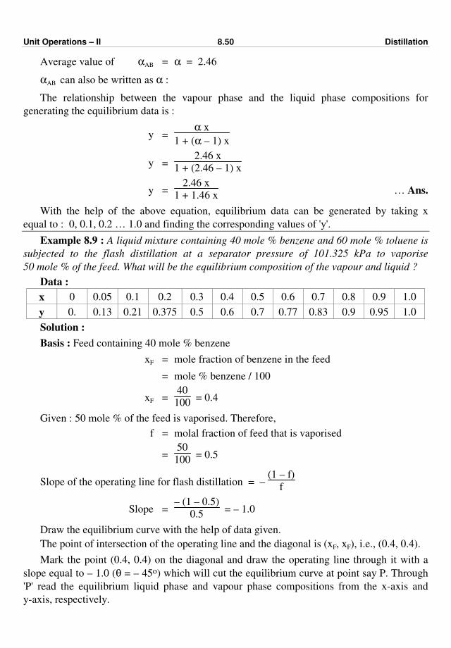
Unit Operations – II 8.50 Distillation
Average value of αAB = α = 2.46
αAB can also be written as α :
The relationship between the vapour phase and the liquid phase compositions for
generating the equilibrium data is :
y = α x
1 + (α – 1) x
y = 2.46 x
1 + (2.46 – 1) x
y = 2.46 x
1 + 1.46 x … Ans.
With the help of the above equation, equilibrium data can be generated by taking x
equal to : 0, 0.1, 0.2 … 1.0 and finding the corresponding values of 'y'.
Example 8.9 : A liquid mixture containing 40 mole % benzene and 60 mole % toluene is
subjected to the flash distillation at a separator pressure of 101.325 kPa to vaporise
50 mole % of the feed. What will be the equilibrium composition of the vapour and liquid ?
Data :
x 0 0.05 0.1 0.2 0.3 0.4 0.5 0.6 0.7 0.8 0.9 1.0
y 0. 0.13 0.21 0.375 0.5 0.6 0.7 0.77 0.83 0.9 0.95 1.0
Solution :
Basis : Feed containing 40 mole % benzene
xF = mole fraction of benzene in the feed
= mole % benzene / 100
xF = 40
100 = 0.4
Given : 50 mole % of the feed is vaporised. Therefore,
f = molal fraction of feed that is vaporised
= 50
100 = 0.5
Slope of the operating line for flash distillation = – (1 – f)
f
Slope = – (1 – 0.5)
0.5 = – 1.0
Draw the equilibrium curve with the help of data given.
The point of intersection of the operating line and the diagonal is (xF, xF), i.e., (0.4, 0.4).
Mark the point (0.4, 0.4) on the diagonal and draw the operating line through it with a
slope equal to – 1.0 (θ = – 45o) which will cut the equilibrium curve at point say P. Through
'P' read the equilibrium liquid phase and vapour phase compositions from the x-axis and
y-axis, respectively.
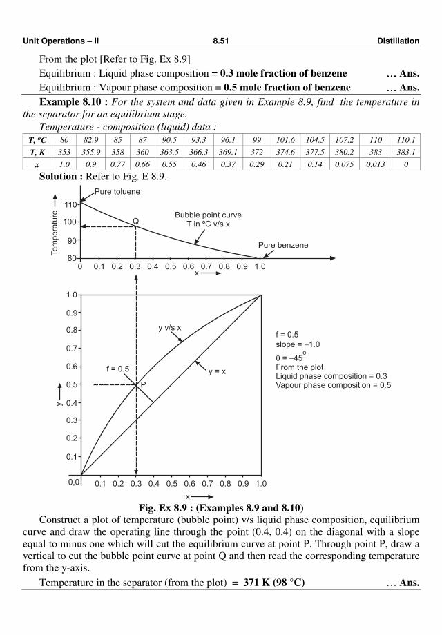
Unit Operations – II 8.51 Distillation
From the plot [Refer to Fig. Ex 8.9]
Equilibrium : Liquid phase composition = 0.3 mole fraction of benzene ………… Ans.
Equilibrium : Vapour phase composition = 0.5 mole fraction of benzene ………… Ans.
Example 8.10 : For the system and data given in Example 8.9, find the temperature in
the separator for an equilibrium stage.
Temperature - composition (liquid) data :
T, oC 80 82.9 85 87 90.5 93.3 96.1 99 101.6 104.5 107.2 110 110.1
T, K 353 355.9 358 360 363.5 366.3 369.1 372 374.6 377.5 380.2 383 383.1
x 1.0 0.9 0.77 0.66 0.55 0.46 0.37 0.29 0.21 0.14 0.075 0.013 0
Solution : Refer to Fig. E 8.9.
80
90
100
110
Te
mp
era
ture
Pure toluene
Q
0 0.1 0.2 0.3 0.4 0.5 0.6 0.7 0.8 0.9 1.0
Pure benzene
Bubble point curveT in ºC v/s x
x
0,0 0.1 0.2 0.3 0.4 0.5 0.6 0.7 0.8 0.9 1.0
x
P
f = 0.5 y = x
y v/s x
1.0
0.1
0.2
0.3
0.4
0.5
0.6
0.7
0.8
0.9
y
f = 0.5
slope = 1.0
= 45From the plotLiquid phase composition = 0.3Vapour phase composition = 0.5
-
q -o
Fig. Ex 8.9 : (Examples 8.9 and 8.10)
Construct a plot of temperature (bubble point) v/s liquid phase composition, equilibrium
curve and draw the operating line through the point (0.4, 0.4) on the diagonal with a slope
equal to minus one which will cut the equilibrium curve at point P. Through point P, draw a
vertical to cut the bubble point curve at point Q and then read the corresponding temperature
from the y-axis.
Temperature in the separator (from the plot) = 371 K (98 °C) … Ans.

Unit Operations – II 8.52 Distillation
Example 8.11 : A liquid mixture containing 40 mole % methanol and 60 mole % water is
fed to a differential distillation at atmospheric pressure, with 60 mole % of the liquid is
distilled. Find the composition of the composited distillate and the residue.
Equilibrium data :
x 0.05 0.1 0.2 0.3 0.4 0.5
y 0.27 0.42 0.57 0.66 0.73 0.78
Solution :
Basis : 100 kmol of feed
Let F, D, W be the kmol of the feed, distillate and residue, respectively.
Given : 60 mole % of the feed is distilled
∴ D = 0.60 × 100 = 60 kmol
We know F = D + W
100 = 60 + W
∴ W = 40 kmol
xF = mole fraction of methanol in the feed
xF = 40
100 = 0.4
xW = mole fraction of methanol in the residue left in the still
Rayleigh equation is :
ln
F
W = ⌡⌠
xW
xF
dx
y – x
R.H.S. of this equation is evaluated graphically by plotting 1/y–x as ordinate v/s x as
abscissa and measuring the area under the curve between the limits x = xF and x = xW.
L.H.S. of the Rayleigh equation = ln
F
W = ln
100
40 = 0.916
Plot 1/(y – x) v/s x and measure the area under the curve from xF = 0.50 till the area
equals 0.916 and then read the value of x representing xW (composition of the residue).
x 0.05 0.1 0.2 0.3 0.4 0.5
y 0.27 0.42 0.57 0.66 0.73 0.78
1/y – x 4.54 3.12 2.7 2.8 3.0 3.6
From Fig. Ex 8.11, xW = 0.075 mole fraction of methanol in the residue. … Ans.
yDavg – composited distillate composition.

Unit Operations – II 8.53 Distillation
Methanol material balance :
xF · F = yD, avg. · D + xW · W
0.40 × 100 = yD, avg. (60) + 0.075 × 40
yD, avg. = 0.62 … Ans.
Scale : Refer Fig. Ex 8.11.
x-axis : 20 mm = 0.1 units
y-axis : 20 mm = 1.0 units
ln F
W = ⌡⌠
xF
xW
dx
y – x
0.916 = Area (x-axis scale) (y-axis scale)
0.96 = Area
0.1
2 1
2
Area = 36.64 cm2
Measure the area under the curve from xF = 0.4 till we get : area = 36.64 cm2 and read xW
from the x-axis.
∴ From Fig. Ex 8.11, xW = 0.075 mole fraction of methanol in the residue.
xW = 0.075 … Ans.
8
7
6
5
4
3
2
1
0,0
1/(
yx)
-
1.00.90.80.70.60.50.40.30.20.1
x
Measure area
x = 0.075w x = 0.40F
Fig. Ex 8.11
Example 8.12 : 100 kmol/h of a feed containing 35 mole % methanol is to be
continuously distilled in a fractionating column to get 96.5 mole % methanol as a distillate
and 10 mole % methanol as a bottom product. Find the molal flow rates of the distillate and
the bottoms.
Unit Operations – II 8.54 Distillation
Solution : Basis : 100 kmol/h of feed
xF = mole fraction of methanol in the feed
= 36
100 = 0.36
xD = mole fraction of methanol in distillate
= 96.5
100 = 0.965
xW = mole fraction of methanol in bottoms
= 10
100 = 0.1
Let F, D and W be the molal flow rates, in kmol/h, of the feed, distillate and bottom
product, respectively.
Overall material balance :
F = D + W
Material balance of methanol :
xF · F = xD · D + xW · W
Substituting the values of F, xD, xW, and xF in above equations
100 = D + W
D = 100 – W
∴ 0.36 × 100 = 0.965 D + 0.1 W
36 = 0.965 (100 – W) + 0.1 W
∴ W = 69.95 kmol/h ………… Ans.
and D = 30.05 kmol/h … Ans.
Example 8.13 : A feed containing 40 mole % benzene and 60 mole % toluene is to be
distilled in a fractionating column to get a top product (distillate) containing 90 mole %
benzene and a bottom product containing not more than 10 mole % benzene. The reflux ratio
of 3 kmol per kmol of product is used. Assuming feed to be a liquid at its bubble point
(saturated liquid), find the number of theoretical plates required and the position of the feed
plate by Lewis-Sorel method.
Equilibrium data :
x 0 0.05 0.1 0.2 0.3 0.4 0.5 0.6 0.7 0.8 0.9 1
y 0 0.13 0.21 0.375 0.5 0.6 0.7 0.77 0.83 0.9 0.95 1
Solution : Basis : 100 kmol of feed to the column
Overall material balance :
F = D + W
F = 100 = D + W … (A)
Mole fraction of benzene in the feed = mole % benzene in the feed
100
xF = 0.4
Unit Operations – II 8.55 Distillation
Similarly, the mole fractions of benzene in the distillate and the residue are :
xD = 0.9 and xW = 0.1
Material balance of benzene :
xF · F = xD · D + xW · W
0.4 × 100 = 0.9 D + 0.1 W
40 = 0.9 D + 0.1 W
From Equation (A), D = 100 – W
∴ 40 = 0.9 (100 – W) + 0.1 W
Solving, we get W = 62.5 kmol
and D = 37.5 kmol
R = Reflux ratio = 3 = L
D
but L = Ln
∴ Ln = 3 D
Ln = 3 (37.5)
= 112.5 kmol
Ln + D = 112.5 + 37.5 = 150 kmol
The rectifying section operating line is
xn+1 = Ln
Ln + D xn +
D · xD
Ln + D
∴ yn+1 = 112.5 xn
150 +
37.5 × 0.9
150 … (B)
yn+1 = 0.75 xn + 0.225
Since the feed is a liquid at its bubble point, we have
Lm = Ln + F
= 112.5 + 100 = 212.5 kmol
and Lm – W = 212.5 – 62.5 = 150 kmol
The operating line of the stripping section is
ym+1 = Lm
Lm – W xm –
W
Lm – W xW
ym+1 = 212.5
150 xm –
62.5
150 × 0.1
ym+1 = 1.415 xm – 0.042 … (C)
Distillate composition = xD = 0.9
∴ yn = xD = 0.9
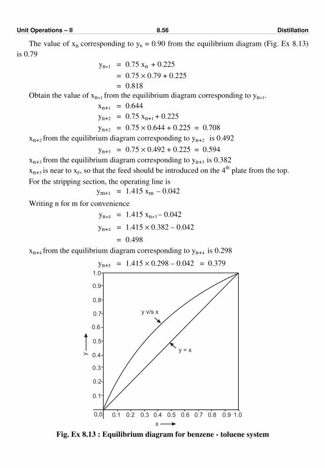
Unit Operations – II 8.56 Distillation
The value of xn corresponding to yn = 0.90 from the equilibrium diagram (Fig. Ex 8.13)
is 0.79
yn+1 = 0.75 xn + 0.225
= 0.75 × 0.79 + 0.225
= 0.818
Obtain the value of xn+1 from the equilibrium diagram corresponding to yn+1.
xn+1 = 0.644
yn+2 = 0.75 xn+1 + 0.225
yn+2 = 0.75 × 0.644 + 0.225 = 0.708
xn+2 from the equilibrium diagram corresponding to yn+2 is 0.492
yn+3 = 0.75 × 0.492 + 0.225 = 0.594
xn+3 from the equilibrium diagram corresponding to yn+3 is 0.382
xn+3 is near to xF, so that the feed should be introduced on the 4th
plate from the top.
For the stripping section, the operating line is
ym+1 = 1.415 xm – 0.042
Writing n for m for convenience
yn+4 = 1.415 xn+3 – 0.042
yn+4 = 1.415 × 0.382 – 0.042
= 0.498
xn+4 from the equilibrium diagram corresponding to yn+4 is 0.298
yn+5 = 1.415 × 0.298 – 0.042 = 0.379
0.1 0.2 0.3 0.4 0.5 0.6 0.7 0.8 0.9 1.0
x
0,0
0.1
0.2
0.3
0.4
0.5
0.6
0.7
0.8
0.9
1.0
y v/s x
y = x
y
Fig. Ex 8.13 : Equilibrium diagram for benzene - toluene system

Unit Operations – II 8.57 Distillation
xn+5 from the equilibrium diagram is 0.208
yn+6 = 1.4165 × 0.208 – 0.042 = 0.252
xn+6 from the equilibrium diagram is equal to 0.120
yn+7 = 1.415 × 0.120 – 0.042 = 0.127
xn+7 from the equilibrium diagram is equal to 0.048.
[As xn+6 = 0.12 greater than xW = 0.1, one more step is incorporated so that the liquid
phase composition obtained at any case should not be more than xW.]
Hence, there will be 7 plates in the column. … Ans.
Example 8.14 : A mixture of benzene and toluene containing 60 mole % benzene is
to be separated to give a product of 95 mole % benzene and a bottom product containing
10 mole % benzene. The feed enters a column at its bubble point. It is proposed to operate
the column with reflux ratio of 2.5. It is required to find the number of theoretical plates
needed and the position of feed plate. Equilibrium data :
x 0 0.05 0.1 0.2 0.3 0.4 0.5 0.6 0.7 0.8 0.9 1.0
y 0 0.13 0.21 0.375 0.5 0.6 0.7 0.77 0.83 0.9 0.95 1.0
Solution : Basis : Feed containing 60 mole % benzene
xF = mole fraction of benzene in the feed
= mole % benzene / 100
= 60
100 = 0.60
xD = mole fraction of benzene in the top product
= 95
100 = 0.95
xW = mole fraction of benzene in the bottom product
= 10
100 = 0.1
McCabe-Thiele method is used.
The operating line of the rectification section is having slope of R/R + 1, and intercept on
y-axis equal to xD/R + 1. The point of intersection of the operating line of the rectification
section and the diagonal is – (xD, xD).
Slope of the operating line = R/R + 1
where R = Reflux ratio = 2.5
∴ Slope = 2.5
2.5 + 1 = 0.714
Intercept = xD
R + 1 =
0.95
(2.5 + 1) = 0.271
With the help of given vapour-liquid equilibrium data, construct a plot of y v/s x.
Point of intersection of this operating line with the diagonal is
(xD, xD) ⇒ (0.95, 0.95)
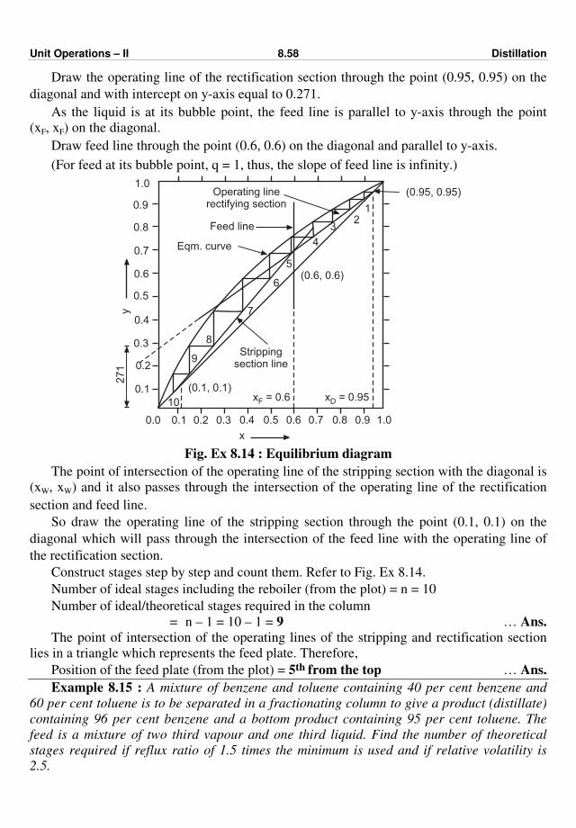
Unit Operations – II 8.58 Distillation
Draw the operating line of the rectification section through the point (0.95, 0.95) on the
diagonal and with intercept on y-axis equal to 0.271.
As the liquid is at its bubble point, the feed line is parallel to y-axis through the point
(xF, xF) on the diagonal.
Draw feed line through the point (0.6, 0.6) on the diagonal and parallel to y-axis.
(For feed at its bubble point, q = 1, thus, the slope of feed line is infinity.)
0.0 0.1 0.2 0.3 0.4 0.5 0.6 0.7 0.8 0.9 1.0
0.1
0.2
0.3
0.4
0.5
0.6
0.7
0.8
0.9
1.0
27
1y
10
9
8
7
(0.1, 0.1)
Eqm. curve
Feed line
Operating linerectifying section
(0.6, 0.6)6
5
4
32
1
Strippingsection line
x = 0.6F x = 0.95D
(0.95, 0.95)
x
Fig. Ex 8.14 : Equilibrium diagram
The point of intersection of the operating line of the stripping section with the diagonal is
(xW, xW) and it also passes through the intersection of the operating line of the rectification
section and feed line.
So draw the operating line of the stripping section through the point (0.1, 0.1) on the
diagonal which will pass through the intersection of the feed line with the operating line of
the rectification section.
Construct stages step by step and count them. Refer to Fig. Ex 8.14.
Number of ideal stages including the reboiler (from the plot) = n = 10
Number of ideal/theoretical stages required in the column
= n – 1 = 10 – 1 = 9 … Ans.
The point of intersection of the operating lines of the stripping and rectification section
lies in a triangle which represents the feed plate. Therefore,
Position of the feed plate (from the plot) = 5th from the top … Ans.
Example 8.15 : A mixture of benzene and toluene containing 40 per cent benzene and
60 per cent toluene is to be separated in a fractionating column to give a product (distillate)
containing 96 per cent benzene and a bottom product containing 95 per cent toluene. The
feed is a mixture of two third vapour and one third liquid. Find the number of theoretical
stages required if reflux ratio of 1.5 times the minimum is used and if relative volatility is
2.5.
Unit Operations – II 8.59 Distillation
Solution : Basis : Feed containing 40% benzene and 60% toluene (by wt.)
Molecular weight of benzene = 78
Molecular weight of toluene = 92
xF = mole fraction of benzene in the feed
=
40
78
40
78 +
60
92
= 0.44
Similarly, xD = mole fraction of benzene in the distillate
=
96
78
96
78 +
4
92
= 0.966
xW = mole fraction of benzene in the bottom product
=
5
78
5
78 +
95
92
= 0.058
Relative volatility = α = 2.5
With the help of relative volatility, generate x–y data and plot y v/s x.
For generating x-y data, assume x = 0, 0.1, 0.2, … 1 and find the corresponding values
of y from the relation :
y = α x
1 + (α – 1) x
For x = 0
y = 2.5 (0)
1 + (2.5 – 1) 0 = 0
For x = 0.1
y = 2.5 × 0.1
1 + (2.5 – 1) 0.1 = 0.22
Similarly, evaluate values of y for the remaining values of x.
x 0 0.1 0.2 0.3 0.4 0.5 0.6 0.7 0.8 0.9 1.0
y 0 0.22 0.385 0.52 0.625 0.714 0.79 0.85 0.91 0.96 1.0

Unit Operations – II 8.60 Distillation
Procedure for finding out minimum reflux ratio :
Given : Feed is 2/3rd vapour and 1/3rd liquid.
We have : q = fraction of the feed that is liquid
∴ q = 1
3 = 0.333
or q = 1 – f, where f - fraction of the feed that is vaporised
∴ q = 1 – 2
3 = 1 – 0.667 = 0.333
Slope of the feed line = –
q
1 – q
= (– 0.333)
(1 – 0.333) = – 0.5
Slope = tan θ = – 0.5
θ = – 26.56o
Intercept on y-axis = xF
1 – q
= 0.44
(1 – 0.333)
= 0.66
Draw a feed line through the point (0.44, 0.44) on the diagonal with slope equal to
– 0.5 (with an angle equal to – 26.56o) or with intercept equal to 0.66 which will cut the
equilibrium curve at point P. Through the point A (0.966, 0.966) on the diagonal, draw the
operating line A – P of the rectification section (dotted line) and read y' and x' from the
y-axis and x-axis, respectively. [Which represents the condition for a minimum reflux].
Minimum reflux ratio = Rm = xD – y'
y' – x'
from the plot, y' = 0.515, x' = 0.3
Rm = 0.966 – 0.515
0.515 – 0.3 = 2.1
Given : Operating reflux ratio = R = 1.5 Rm
R = 1.5 × 2.1 = 3.14
Operating line of rectification section :
Point A (0.966, 0.966) on the diagonal.
Intercept of the rectifying section operating line is
= xD
R + 1
= 0.966
3.14 + 1 = 0.232

Unit Operations – II 8.61 Distillation
Draw the operating line of the rectifying section on the x-y diagram through the
point A (0.966, 0.966) with intercept on y-axis equal to 0.232. Draw operating line of the
stripping section starting from the point (0.0581, 0.058) on the diagonal passing through the
point Q (the point of intersection of the feed line and rectifying section line).
Do step by step construction of stages between the equilibrium curve and the operating
lines starting from the point A upto point B and count the number of stages.
From the plot (Fig. Ex 8.15) :
Number of theoretical stages required including the reboiler = n = 10
Number of theoretical stages required in the column = n – 1 = 10 – 1 = 9 … Ans.
y
0.0 0.1 0.2 0.3 0.4 0.5 0.6 0.7 0.8 0.9 1.0
0.1
0.2
0.3
0.4
0.5
0.6
0.7
0.8
0.9
1.0
Feed line
y v/s x
P
QOperating line
y = x
xD
A(0.966, 0.966)1
2
3
4
5
6
78
9
(0.058,0.058) x = 0.44F
From the plot:
y' = 0.515
x = 0.30
Number of theoretical
plates including reboiler = 10
x
Fig. Ex 8.15 : Equilibrium Diagram
Example 8.16 : A methanol (A) – water (B) solution containing 50 % by weight
methanol at 300 K (27o C) is to be continuously rectified at 101.325 kPa at a rate of
5000 kg/h to provide a distillate containing 95 % methanol and a residue containing
1.0 % methanol (by weight). Calculate the flow rates of the distillate and residue on
(i) weight basis and (ii) mole basis.
Solution : Basis : (i) 5000 kg/h of methanol-water solution.
Let x'F , x
'D and x
'W
be the weight fractions of methanol in the feed, distillate and residue
respectively. Let F', D' and W' be the kg/h of the feed, distillate and residue, respectively.
Overall material balance :
F' = D' + W'
5000 = D' + W' ∴ W' = 5000 – D'
Material balance of methanol :
x'F F' = x
'D D' + x
'W
W'
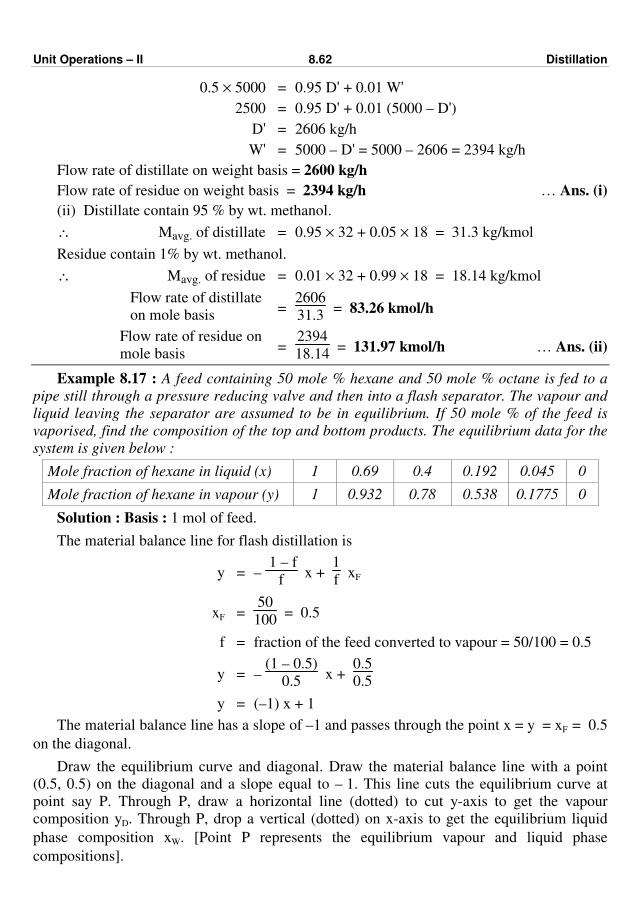
Unit Operations – II 8.62 Distillation
0.5 × 5000 = 0.95 D' + 0.01 W'
2500 = 0.95 D' + 0.01 (5000 – D')
D' = 2606 kg/h
W' = 5000 – D' = 5000 – 2606 = 2394 kg/h
Flow rate of distillate on weight basis = 2600 kg/h
Flow rate of residue on weight basis = 2394 kg/h … Ans. (i)
(ii) Distillate contain 95 % by wt. methanol.
∴ Mavg. of distillate = 0.95 × 32 + 0.05 × 18 = 31.3 kg/kmol
Residue contain 1% by wt. methanol.
∴ Mavg. of residue = 0.01 × 32 + 0.99 × 18 = 18.14 kg/kmol
Flow rate of distillate
on mole basis = 2606
31.3 = 83.26 kmol/h
Flow rate of residue on
mole basis = 2394
18.14 = 131.97 kmol/h … Ans. (ii)
Example 8.17 : A feed containing 50 mole % hexane and 50 mole % octane is fed to a
pipe still through a pressure reducing valve and then into a flash separator. The vapour and
liquid leaving the separator are assumed to be in equilibrium. If 50 mole % of the feed is
vaporised, find the composition of the top and bottom products. The equilibrium data for the
system is given below :
Mole fraction of hexane in liquid (x) 1 0.69 0.4 0.192 0.045 0
Mole fraction of hexane in vapour (y) 1 0.932 0.78 0.538 0.1775 0
Solution : Basis : 1 mol of feed.
The material balance line for flash distillation is
y = – 1 – f
f x +
1
f xF
xF = 50
100 = 0.5
f = fraction of the feed converted to vapour = 50/100 = 0.5
y = – (1 – 0.5)
0.5 x +
0.5
0.5
y = (–1) x + 1
The material balance line has a slope of –1 and passes through the point x = y = xF = 0.5
on the diagonal.
Draw the equilibrium curve and diagonal. Draw the material balance line with a point
(0.5, 0.5) on the diagonal and a slope equal to – 1. This line cuts the equilibrium curve at
point say P. Through P, draw a horizontal line (dotted) to cut y-axis to get the vapour
composition yD. Through P, drop a vertical (dotted) on x-axis to get the equilibrium liquid
phase composition xW. [Point P represents the equilibrium vapour and liquid phase
compositions].
Unit Operations – II 8.63 Distillation
From Fig. Ex. 8.17 :
Composition of vapour and liquid from the flash separator :
Composition of top product (vapour) = 0.69 × 100 = 69 mole % hexane.
Composition of bottom product (liquid) = 0.31 × 100 = 31 mole % hexane. ………… Ans.
y v/s x
1.0
0.9
0.8
0.7
0.6
0.5
0.4
0.3
0.2
0.1
1.00.90.80.70.60.50.40.30.20.10,0
y
y = x
x
P
x =0.31W x = 0.5F
Fig. Ex 8.17
Example 8.18 : A feed containing 60 mole % hexane and 40 mole % octane is fed to a
pipe still through a pressure reducing valve into a flash separator. The vapour and liquid
leaving the separator are assumed to be in equilibrium. If 50 mole % of the feed is vaporised,
find the composition of the top and bottom products. The equilibrium data is given below.
x, mole fraction of hexane in liquid 1.0 0.69 0.40 0.192 0.045 0
y, mole fraction of hexane in vapour 1.0 0.932 0.78 0.538 0.1775 0
Solution : Basis : 1 kmol of feed.
xF = mole fraction of n-hexane in the feed = 60
100 = 0.60
Feed is 50 mole % vaporised
∴ f = 50
100 = 0.5
f-fraction of feed converted to vapour = 0.5
1 = 0.5
Operating line for flash distillation is
y = – (1 – f)
f x +
xF
f
slope = – (1 – f)/f
= – (1.0 – 0.5)/0.5 = – 1
The point of intersection of the operating line with the diagonal is (0.6, 0.6).
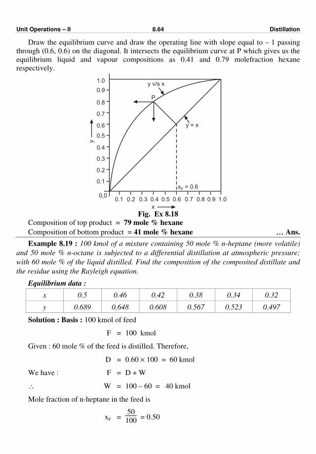
Unit Operations – II 8.64 Distillation
Draw the equilibrium curve and draw the operating line with slope equal to – 1 passing
through (0.6, 0.6) on the diagonal. It intersects the equilibrium curve at P which gives us the
equilibrium liquid and vapour compositions as 0.41 and 0.79 molefraction hexane
respectively.
y v/s x1.0
0.9
0.8
0.7
0.6
0.5
0.4
0.3
0.2
0.1
1.00.90.80.70.60.50.40.30.20.10,0
y
y = x
x
P
x = 0.6F
Fig. Ex 8.18
Composition of top product = 79 mole % hexane
Composition of bottom product = 41 mole % hexane ………… Ans.
Example 8.19 : 100 kmol of a mixture containing 50 mole % n-heptane (more volatile)
and 50 mole % n-octane is subjected to a differential distillation at atmospheric pressure;
with 60 mole % of the liquid distilled. Find the composition of the composited distillate and
the residue using the Rayleigh equation.
Equilibrium data :
x 0.5 0.46 0.42 0.38 0.34 0.32
y 0.689 0.648 0.608 0.567 0.523 0.497
Solution : Basis : 100 kmol of feed
F = 100 kmol
Given : 60 mole % of the feed is distilled. Therefore,
D = 0.60 × 100 = 60 kmol
We have : F = D + W
∴ W = 100 – 60 = 40 kmol
Mole fraction of n-heptane in the feed is
xF = 50
100 = 0.50
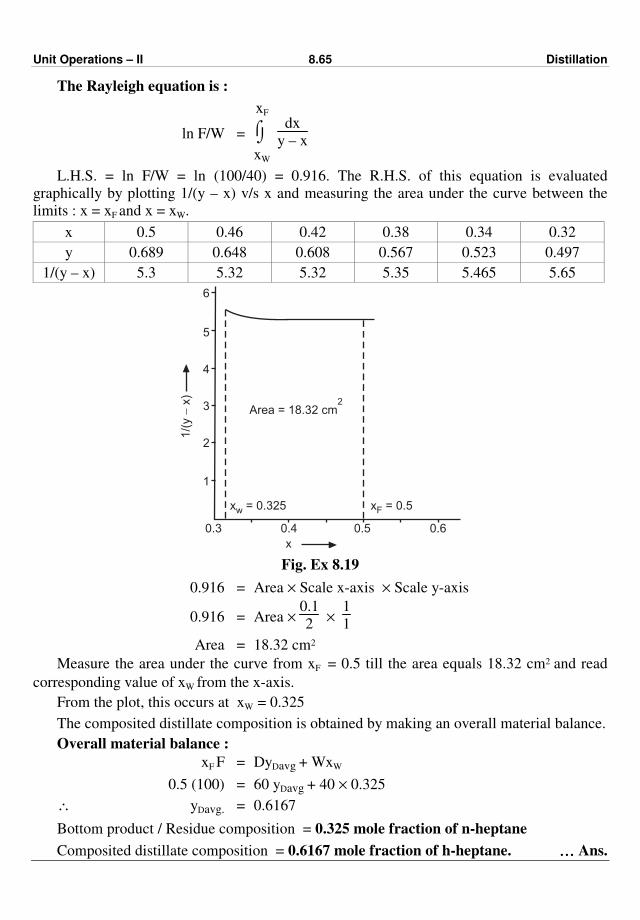
Unit Operations – II 8.65 Distillation
The Rayleigh equation is :
ln F/W = ⌡⌠
xW
xF
dx
y – x
L.H.S. = ln F/W = ln (100/40) = 0.916. The R.H.S. of this equation is evaluated
graphically by plotting 1/(y – x) v/s x and measuring the area under the curve between the
limits : x = xF and x = xW.
x 0.5 0.46 0.42 0.38 0.34 0.32
y 0.689 0.648 0.608 0.567 0.523 0.497
1/(y – x) 5.3 5.32 5.32 5.35 5.465 5.65
0.3 0.4 0.5 0.6
x = 0.5Fx = 0.325w
1
2
3
4
5
6
1/(
yx)
- Area = 18.32 cm2
x
Fig. Ex 8.19
0.916 = Area × Scale x-axis × Scale y-axis
0.916 = Area × 0.1
2 ×
1
1
Area = 18.32 cm2
Measure the area under the curve from xF = 0.5 till the area equals 18.32 cm2 and read
corresponding value of xW from the x-axis.
From the plot, this occurs at xW = 0.325
The composited distillate composition is obtained by making an overall material balance.
Overall material balance :
xF F = DyDavg + WxW
0.5 (100) = 60 yDavg + 40 × 0.325
∴ yDavg. = 0.6167
Bottom product / Residue composition = 0.325 mole fraction of n-heptane
Composited distillate composition = 0.6167 mole fraction of h-heptane. ………… Ans.
Unit Operations – II 8.66 Distillation
Example 8.20 : A fractionating column is designed to separate 15000 kg/h of a feed
containing 60% toluene and 40% benzene into an overhead product containing 97% benzene
and a waste containing 98% toluene. All % are by weight. Calculate the weights of the
product and waste product per hour.
Solution : Basis : 15000 kg/h of feed to the distillation column.
F' = 15000 kg/h
D' = product, kg/h
W' = waste product, kg/h
x'F = wt. fraction of benzene in the feed =
40
100 = 0.40
x'D = wt. fraction of benzene in the product =
97
100 = 0.97
x'W
= wt. fraction of benzene in the waste product = 2
100 = 0.02
Overall material balance :
F' = W' + D'
30,000 = W' + D'
W' = 15000 – D'
Material balance of benzene :
x'F F = x
'D D' + x
'W
W'
0.4 (15000) = 0.97 D' + 0.02 W'
Replacing W' by 15000 – D' gives
6000 = 0.97 D' + 0.02 (15000 – D')
∴ D' = 6000
W' = 15000 – 6000 = 9000 kg/h
Distillate/Product flow rate = 6000 kg/h
Bottom/Waste product flow rate = 9000 kg/h … Ans.
Example 8.21 : A liquid mixture has a relative volatility of 2.5. Compute the vapour-
liquid equilibria for the liquid mixture.
The above mentioned liquid mixture is fed to a distillation column for separation
purpose. Feed is a liquid at its bubble point containing 50 mole % of A (the more volatile
component). The product/distillate is to contain 95 mole % of A and residue is to contain
10 mole % of A. Reflux ratio is 2.5. Calculate the number of ideal plates required and the
position of feed plate.
Solution : Relative volatility = α = 2.5
y = α x
1 + (α – 1) x
y = 2.5 x
1 + (2.5 – 1) x =
2.5 x
1 + 1.5 x

Unit Operations – II 8.67 Distillation
Evaluate y at different values of x and tabulate.
For x = 0 ∴ y = 0
For x = 0.10
y = 2.5 × 0.1
1 + 1.5 × 0.1 = 0.217
x 0 0.1 0.2 0.3 0.4 0.5 0.6 0.7 0.8 0.9 1
y 0 0.217 0.385 0.52 0.62 0.714 0.79 0.85 0.91 0.96 1
xF = mole fraction of A in the feed = 50/100 = 0.50
Similarly, xD = 95
100 = 0.95
and xW = 10
100 = 0.10
Draw the equilibrium curve. Draw the operating lines. The operating line of the
rectification section has a point (xD, xD) on the diagonal.
Intercept of the operating line
of rectification section = xD
R + 1 =
0.95
2.5 + 1 = 0.2714
The point of intersection of the feed line with the diagonal is (xF, xF) i.e. (0.5, 0.5) and
this line is parallel to y-axis through it as the feed is a liquid at its bubble point.
Point of intersection of the operating line for the stripping section with the diagonal is
(xW, xW) i.e. (0.1, 0.1). First draw the operating line of the rectifying section through the point
(0.95, 0.95) on the diagonal and with an intercept on y-axis equal to 0.2714, then draw a feed
line through point (0.5, 0.5) on the diagonal and parallel to y-axis. Then draw the operating
line of stripping section through point (0.1, 0.1) on the diagonal and passing through the
intersection of the rectification section line and the feed line. Construct stages representing
ideal plates between the operating lines and equilibrium curve starting from (0.95, 0.95) till
we reach or cover point (0.1, 0.1) and count them.
0.0 0.1 0.2 0.3 0.4 0.5 0.6 0.7 0.8 0.9 1.0
0.1
0.2
0.3
0.4
0.5
0.6
0.7
0.8
0.9
1.0
y
10
9
8
7
(0.1, 0.1)
Feed line
6
5
4
3
2
1
Strippingsection line
x = 0.5F
xD
(0.95, 0.95)
y v/s x
Rectifyingsection line
y = x
I = 0.2714I = Intercept
x
Fig. Ex 8.21

Unit Operations – II 8.68 Distillation
From the plot :
Number of ideal plates including the reboiler = n = 8
Number of ideal plates in the column = n – 1 = 7.
Position of the feed plate = 5th from the top.
Example 8.22 : A rectification column is fed with 100 kmol/h of a mixture containing
50 mole % hexane and 50 mole % octane at 101.325 kPa absolute pressure. The feed is at its
boiling point. The distillate is to contain 90 mole % hexane and the bottoms 10 mole %
hexane. The reflux ratio is 3 : 1. Calculate the kmol/h distillate and kmol/h bottoms, and the
number of theoretical trays needed for this separation. The equilibrium data for this system
is given below.
Mole fraction of hexane in liquid, x 1.0 0.69 0.4 0.192 0.045 0
Mole fraction of hexane in vapour, y 1.0 0.932 0.78 0.538 0.1775 0
Solution : Basis : 100 kmol/h of feed mixture
F = 100 kmol/h
The feed contains 50 mole % hexane. Therefore,
xF = 0.5 mole fraction of hexane in the feed
Similarly, xD = 0.90
and xW = 0.10
Overall material balance :
F = D + W
Material balance of hexane :
xF F = xD D + xW W
0.5 × 100 = 0.9 D + 0.1 W
100 = D + W
W = 100 – D
50 = 0.9 D + 0.1 (100 – D)
Solving, we get
D = 50 kmol/h
∴ W = 100 – 50 = 50 kmol/h
Distillate = 50 kmol/h
Bottom product = 50 kmol/h ………… Ans.
Draw the equilibrium curve using the data provided.
xF = 0.5 mole fraction of hexane.
Since the feed is at its bubble point, the feed line is parallel to y-axis through (0.5, 0.5) on
the diagonal.
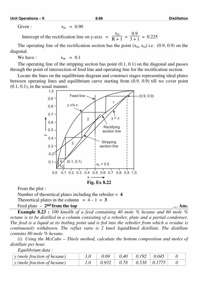
Unit Operations – II 8.69 Distillation
Given : xD = 0.90
Intercept of the rectification line on y-axis = xD
R + 1 =
0.9
3 + 1 = 0.225
The operating line of the rectification section has the point (xD, xD) i.e. (0.9, 0.9) on the
diagonal.
We have : xW = 0.1
The operating line of the stripping section has point (0.1, 0.1) on the diagonal and passes
through the point of intersection of feed line and operating line for the rectification section.
Locate the lines on the equilibrium diagram and construct stages representing ideal plates
between operating lines and equilibrium curve starting from (0.9, 0.9) till we cover point
(0.1, 0.1), in the usual manner.
0.0 0.1 0.2 0.3 0.4 0.5 0.6 0.7 0.8 0.9 1.0
0.1
0.2
0.3
0.4
0.5
0.6
0.7
0.8
0.9
1.0
y
10
(0.1, 0.1)
Feed line
4
3
2
Strippingsection line
x = 0.5F
(0.9, 0.9)
y v/s x
Rectifyingsection line
y = x
x
1
Fig. Ex 8.22
From the plot :
Number of theoretical plates including the reboiler = 4
Theoretical plates in the column = 4 – 1 = 3
Feed plate – 2nd from the top ………… Ans.
Example 8.23 : 100 kmol/h of a feed containing 40 mole % hexane and 60 mole %
octane is to be distilled in a column consisting of a reboiler, plate and a partial condenser.
The feed is a liquid at its boiling point and is fed into the reboiler from which a residue is
continuously withdrawn. The reflux ratio is 2 kmol liquid/kmol distillate. The distillate
contains 80 mole % hexane.
(i) Using the McCabe – Thiele method, calculate the bottom composition and moles of
distillate per hour.
Equilibrium data :
y (mole fraction of hexane) 1.0 0.69 0.40 0.192 0.045 0
y (mole fraction of hexane) 1.0 0.932 0.78 0.538 0.1775 0
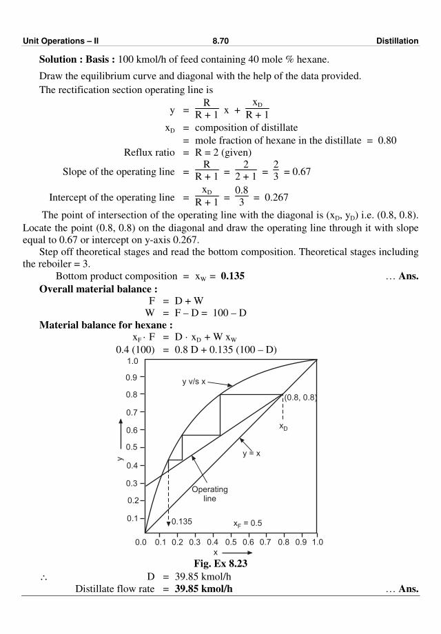
Unit Operations – II 8.70 Distillation
Solution : Basis : 100 kmol/h of feed containing 40 mole % hexane.
Draw the equilibrium curve and diagonal with the help of the data provided.
The rectification section operating line is
y = R
R + 1 x +
xD
R + 1
xD = composition of distillate
= mole fraction of hexane in the distillate = 0.80
Reflux ratio = R = 2 (given)
Slope of the operating line = R
R + 1 =
2
2 + 1 =
2
3 = 0.67
Intercept of the operating line = xD
R + 1 =
0.8
3 = 0.267
The point of intersection of the operating line with the diagonal is (xD, yD) i.e. (0.8, 0.8).
Locate the point (0.8, 0.8) on the diagonal and draw the operating line through it with slope
equal to 0.67 or intercept on y-axis 0.267.
Step off theoretical stages and read the bottom composition. Theoretical stages including
the reboiler = 3.
Bottom product composition = xW = 0.135 … Ans.
Overall material balance : F = D + W
W = F – D = 100 – D
Material balance for hexane : xF · F = D · xD + W xW
0.4 (100) = 0.8 D + 0.135 (100 – D)
0.0 0.1 0.2 0.3 0.4 0.5 0.6 0.7 0.8 0.9 1.0
0.1
0.2
0.3
0.4
0.5
0.6
0.7
0.8
0.9
1.0
y
0.135
Operatingline
x = 0.5F
xD
y v/s x
y = x
x
(0.8, 0.8)
Fig. Ex 8.23
∴ D = 39.85 kmol/h
Distillate flow rate = 39.85 kmol/h … Ans.
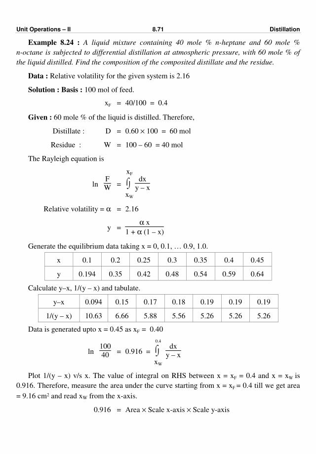
Unit Operations – II 8.71 Distillation
Example 8.24 : A liquid mixture containing 40 mole % n-heptane and 60 mole %
n-octane is subjected to differential distillation at atmospheric pressure, with 60 mole % of
the liquid distilled. Find the composition of the composited distillate and the residue.
Data : Relative volatility for the given system is 2.16
Solution : Basis : 100 mol of feed.
xF = 40/100 = 0.4
Given : 60 mole % of the liquid is distilled. Therefore,
Distillate : D = 0.60 × 100 = 60 mol
Residue : W = 100 – 60 = 40 mol
The Rayleigh equation is
ln F
W = ⌡⌠
xW
xF
dx
y – x
Relative volatility = α = 2.16
y = α x
1 + α (1 – x)
Generate the equilibrium data taking x = 0, 0.1, … 0.9, 1.0.
x 0.1 0.2 0.25 0.3 0.35 0.4 0.45
y 0.194 0.35 0.42 0.48 0.54 0.59 0.64
Calculate y–x, 1/(y – x) and tabulate.
y–x 0.094 0.15 0.17 0.18 0.19 0.19 0.19
1/(y – x) 10.63 6.66 5.88 5.56 5.26 5.26 5.26
Data is generated upto x = 0.45 as xF = 0.40
ln 100
40 = 0.916 = ⌡⌠
xW
0.4
dx
y – x
Plot 1/(y – x) v/s x. The value of integral on RHS between x = xF = 0.4 and x = xW is
0.916. Therefore, measure the area under the curve starting from x = xF = 0.4 till we get area
= 9.16 cm2 and read xW from the x-axis.
0.916 = Area × Scale x-axis × Scale y-axis

Unit Operations – II 8.72 Distillation
0.0 0.1 0.2 0.3 0.4 0.5 0.6 0.7 0.8 0.9 1.0
1/(
y–
x)
1
2
3
4
5
6
7
8
9
10
11
Area
x = 0.22W x = 0.40F
0.916 = Area, cm × ×2
Area = 9.16 cm2
0.1 unit1 cm
1 unit1 cm
x
Fig. Ex 8.24
From Fig. Ex 8.24 : xW = 0.22
Material balance for n-heptane :
F xF = W xW + D yDavg.
100 × 0.40 = 40 × 0.22 + 60 yDavg.
yDavg. = 40 – 8.8
60
= 3.12/60 = 0.52
Therefore, composition of composited distillate = 0.52 mole fraction of heptane.
Composition of residue = 0.22 mole fraction of heptane. … Ans.
Example 8.25 : A mixture of benzene and toluene containing 40 mole % benzene is to be
separated to give a top product of 90 mole % of benzene and a bottom product with not more
than 10 mole % benzene. Using an average value of 2.4 for the volatility of benzene relative
to toluene, calculate the number of theoretical plates required at total reflux.
Also calculate the minimum reflux ratio, if the feed is a liquid at its bubble point.
Solution : Let us generate the x-y data.
Given : Relative volatility = α = 2.4
We know that : y = α x
1 + (α – 1) x =
2.4 x
1 + 1.4 x

Unit Operations – II 8.73 Distillation
For x = 0, 0.1, 0.2 … 1.0, obtain the corresponding values of y and plot the equilibrium
diagram.
x 0 0.1 0.2 0.3 0.4 0.5 0.6 0.7 0.8 0.9 1.0
y 0 0.21 0.375 0.507 0.615 0.706 0.783 0.850 0.906 0.95 1.0
0,0 .1 .2 .3 .4 .5 .6 .7 .8 .9 1.0x
x = 0.4F(0.1, 0.1)
y = x
(0.9, 0.9)
1
2
3
4
5
60.1
0.2
0.3
0.4
0.5
0.6
0.7
0.8
0.9
1.0
P (x , y )F F
y v/s x
y
Fig. E 8.25
Feed contains 40 mole % benzene. Therefore, the mole fraction of benzene in the feed is
xF = 40
100 = 0.40
Similarly, xD = 90
100 = 0.90
and xW = 10
100 = 0.10
To find the plates at total reflux.
Start constructing stages representing ideal plate from the point (0.9, 0.9) till we cover
the point (0.1, 0.1) on the diagonal between the diagonal and equilibrium curve.
Number of plates including the reboiler = n = 6
Number of plates in the column = n – 1 = 6 – 1 = 5
Feed is a liquid at its bubble point. Therefore, draw a feed line through the point
(0.4, 0.4) on the diagonal and parallel to y-axis since for this condition of feed, the feed line
slope is infinity.
The feed line cuts the equilibrium curve at point P (xF, yF).
xF = 0.4, yF = 0.615

Unit Operations – II 8.74 Distillation
The minimum reflux ratio for a saturated feed is given by
Minimum reflux ratio = Rm
Rm = xD – yF
yF – xF
= 0.90 – 0.615
0.615 – 0.40 = 1.325 … Ans.
Example 8.26 : 1000 kmol/h of an ethanol–propanol mixture containing 65 mole percent
ethanol is to be separated in a continuous plate column operating at 101.325 kPa total
pressure. The desired terminal composition in terms of mole fraction of ethanol are
xD = 0.92 and xW = 0.07
The feed is saturated vapour and total condenser is used. When the reflux flow rate is
four times the amount of top product (distillate), find the number of theoretical plates
required for the separation.
Relative volatility of the ethanol-propanol system may be taken as 2.10.
Solution : Given : α = 2.10
Generate the equilibrium data using the relation :
y = α x
1 + (α – 1) x
y = 2.1 x
1 + 1.1 x
Take x = 0, 0.1, 0.2 … 1.0 and find the corresponding values of y.
x 0 0.1 0.2 0.3 0.4 0.5 0.6 0.7 0.8 0.9 1.0
y 0 0.19 0.34 0.47 0.58 0.67 0.76 0.83 0.89 0.95 1.0
Feed contains 65 mole % ethanol. Therefore,
xF = 65
100 = 0.65
Similarly, xD = 0.92 and xW = 0.07
The operating line of the rectification section has point (0.92, 0.92) on the diagonal.
Intercept of this operating line = xD
R + 1
Given : L = reflux fow rate = 4D
∴ L/D = R = 4
Intercept of this operating line = 0.92
4 + 1 = 0.184
Draw the operating line on the equilibrium diagram. Feed is a saturated vapour, therefore
a feed line is parallel to the x-axis and the point of intersection of it with the diagonal is
(0.65, 0.65). Draw the feed line.
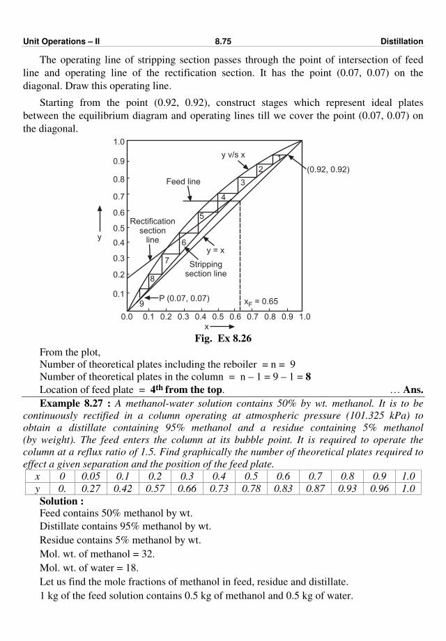
Unit Operations – II 8.75 Distillation
The operating line of stripping section passes through the point of intersection of feed
line and operating line of the rectification section. It has the point (0.07, 0.07) on the
diagonal. Draw this operating line.
Starting from the point (0.92, 0.92), construct stages which represent ideal plates
between the equilibrium diagram and operating lines till we cover the point (0.07, 0.07) on
the diagonal.
y
Feed line
(0.92, 0.92)
1
2
3
4
5
6
7
8
9P (0.07, 0.07)
0.1
0.2
0.3
0.4
0.5
0.6
0.7
0.8
0.9
1.0
0.0 0.1 0.2 0.3 0.4 0.5 0.6 0.7 0.8 0.9 1.0
x
y = x
Strippingsection line
Rectificationsection
line
x = 0.65F
y v/s x
Fig. Ex 8.26
From the plot,
Number of theoretical plates including the reboiler = n = 9
Number of theoretical plates in the column = n – 1 = 9 – 1 = 8
Location of feed plate = 4th from the top. … Ans.
Example 8.27 : A methanol-water solution contains 50% by wt. methanol. It is to be
continuously rectified in a column operating at atmospheric pressure (101.325 kPa) to
obtain a distillate containing 95% methanol and a residue containing 5% methanol
(by weight). The feed enters the column at its bubble point. It is required to operate the
column at a reflux ratio of 1.5. Find graphically the number of theoretical plates required to
effect a given separation and the position of the feed plate.
x 0 0.05 0.1 0.2 0.3 0.4 0.5 0.6 0.7 0.8 0.9 1.0
y 0. 0.27 0.42 0.57 0.66 0.73 0.78 0.83 0.87 0.93 0.96 1.0
Solution : Feed contains 50% methanol by wt.
Distillate contains 95% methanol by wt.
Residue contains 5% methanol by wt.
Mol. wt. of methanol = 32.
Mol. wt. of water = 18.
Let us find the mole fractions of methanol in feed, residue and distillate.
1 kg of the feed solution contains 0.5 kg of methanol and 0.5 kg of water.
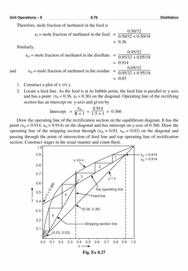
Unit Operations – II 8.76 Distillation
Therefore, mole fraction of methanol in the feed is
xF = mole fraction of methanol in the feed = 0.50/32
0.50/32 + 0.50/18
= 0.36
Similarly,
xD = mole fraction of methanol in the distillate = 0.95/32
0.95/32 + 0.05/18
= 0.914
and xW = mole fraction of methanol in the residue = 0.05/32
0.05/32 + 0.95/18
= 0.03
1. Construct a plot of x v/s y.
2. Locate a feed line. As the feed is at its bubble point, the feed line is parallel to y-axis
and has a point (xF = 0.36, xF = 0.36) on the diagonal. Operating line of the rectifying
section has an intercept on y-axis and given by
Intercept = xD
R + 1 =
0.914
1.5 + 1 = 0.366
Draw the operating line of the rectification section on the equilibrium diagram. It has the
point (xD = 0.914, xD = 0.914) on the diagonal and has intercept on y-axis of 0.366. Draw the
operating line of the stripping section through (xW = 0.03, xW = 0.03) on the diagonal and
passing through the point of intersection of feed line and top operating line of rectification
section. Construct stages in the usual manner and count them.
0.1
0.2
0.3
0.4
0.5
0.6
0.7
0.8
0.9
1.0
0.0 0.1 0.2 0.3 0.4 0.5 0.6 0.7 0.8 0.9 1.0
(0.36, 0.36)
Stripping section line
Feed line
Top operating line
y = x3
I=
0.3
66
y
5
4
(0.03, 0.03)6
x
1
2
y v/s x
x = 0.914D
y = 0.914D
Fig. Ex 8.27

Unit Operations – II 8.77 Distillation
From the plot, total plates including the reboiler = n = 6
Number of plates in the column = n – 1 = 6 – 1 = 5
Feed plate = 4th from the top … Ans.
Example 8.28 : A liquid mixture containing 35 mole % n-heptane and 65 mole %
n-octane (average relative volatility of 2.16) is subjected to a differential distillation
at atmospheric pressure (101.325 kPa), with 65 mole % of the liquid distilled. Estimate the
composition of the composited distillate and residue. Heptane is the more volatile
component.
Solution : Basis : 100 kmol of feed.
Given : 65% of the liquid feed is distilled. Therefore,
D = 0.65 × 100 = 65 kmol
Overall material balance :
F = D + W
∴ W = 100 – 65 = 35 kmol
xF = mole fraction of heptane in the feed = 0.35
xW = mole fraction of heptane in the residue
yD, avg. = mole fraction of heptane in the distillate
The Rayleigh equation is
ln
F
W = ⌡⌠
xW
xF
dx
y – x
LHS = ln
F
W = ln
100
35 = 1.05
Generate : x-y data with the help of α = 2.16
y = αx
1 + (α – 1) x =
2.16 x
1 + (2.16 – 1) x =
2.16 x
1 + 1.16 x
Since xF = 0.35, it is sufficient to generate the data upto x = 0.5.
Take x = 0.05, 0.10, 0.2 … 0.5 and evaluate corresponding values of y.
The RHS of the Rayleigh equation is to be evaluated graphically by plotting 1/(y – x)
against x.
x 0.05 0.10 0.20 0.30 0.40 0.50
y 0.10 0.190 0.35 0.48 0.59 0.68
1/(y – x) 20 11.11 6.67 5.55 5.26 5.55
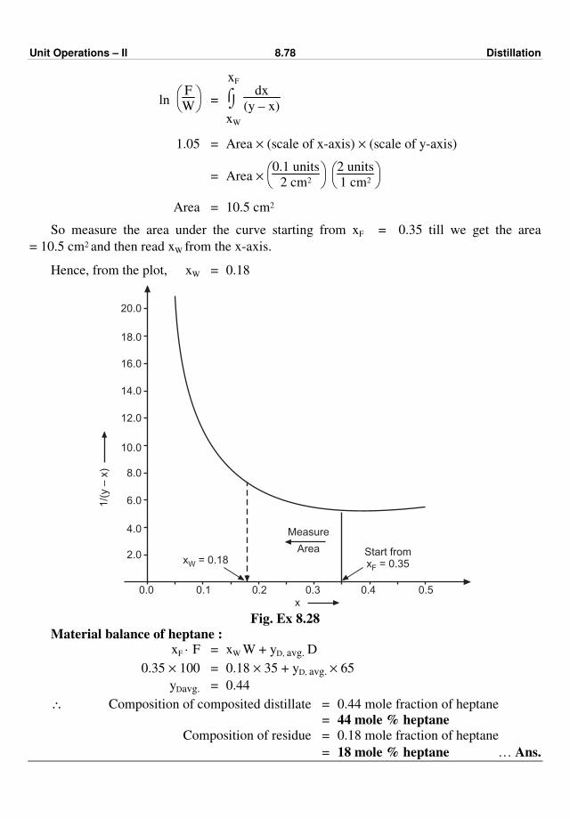
Unit Operations – II 8.78 Distillation
ln
F
W = ⌡⌠
xW
xF
dx
(y – x)
1.05 = Area × (scale of x-axis) × (scale of y-axis)
= Area ×
0.1 units
2 cm2
2 units
1 cm2
Area = 10.5 cm2
So measure the area under the curve starting from xF = 0.35 till we get the area
= 10.5 cm2 and then read xW from the x-axis.
Hence, from the plot, xW = 0.18
0.0 0.1 0.2 0.3 0.4 0.5
Measure
Area
x
2.0
4.0
6.0
8.0
10.0
12.0
14.0
16.0
18.0
20.0
1/(
y–
x)
x = 0.18W
Start fromx = 0.35F
Fig. Ex 8.28
Material balance of heptane : xF · F = xW W + yD, avg. D
0.35 × 100 = 0.18 × 35 + yD, avg. × 65
yDavg. = 0.44
∴ Composition of composited distillate = 0.44 mole fraction of heptane
= 44 mole % heptane
Composition of residue = 0.18 mole fraction of heptane
= 18 mole % heptane … Ans.

Unit Operations – II 8.79 Distillation
EXERCISES
1. Fill in the blanks :
(a) Separation by distillation is not possible when the relative volatility is equal to ..... .
Ans. one
(b) In ……… operation, mass transfer takes place in both the directions. Ans. transfer
(c) The ratio of a vapour pressure of A to the vapour pressure of B is called as ..........
of A with respect to B. Ans. relative volatility
(d) Relative volatility is a measure of separation by ........ Ans. distillation
(e) Distillation utilises the differences in ......... of different components to effect
separation. Ans. vapour pressures
(f) ......... diagrams, are used to see how the equilibrium vapour phase and liquid phase
compositions changes with temperature. Ans. Boiling point
(g) In boiling point diagram, the saturated vapour curve is called as ............ curve.
Ans. dew point
(h) Fractionating column is divided into two section, one is called the rectifying
section and the other is called the ......... section. Ans. stripping
(i) In case of fractionation, the plate on which the feed is introduced is called as .......
plate. Ans. feed
(j) In case of rectification, a part of the condensed liquid that is returned to the column
is called ............... Ans. reflux
(k) Plate column is a stage wise gas-liquid contactor whereas ........ is a differential or
continuous gas-liquid contactor. Ans. packed column
(l) In fractionating column, the liquid from tray above to tray below, flows via ......
Ans. downcomer
2. Define following terms :
(1) Distillation (2) Relative volatility (3) Reflux ratio (4) Volatility
(5) Rectifying section (6) Azeotrope.
3. Write in brief on two principal methods of distillation.
4. State Raoult's law and Dalton's law.
5. Explain briefly the boiling point diagram.
6. Define reflux ratio and write in brief on optimum reflux ratio.
7. When steam distillation is used ?
8. What do you mean by an azeotrope and azeotropic distillation ?
9. Write in brief with sketch on fractionating column.
10. Explain in brief McCabe-Thiele method used for obtaining theoretical plates
required for a given degree of separation.
11. Explain in brief Lewis-Sorel method used to obtain theoretical plates required for a
given degree of separation.
12. What do you mean by H.E.T.P ?
Unit Operations – II 8.80 Distillation
13. Give the equation of operating line for flash distillation and draw its sketch.
14. Draw a neat sketch of differential distillation and explain it in brief.
15. Draw a x–y plot and draw on this plot the operating lines in case of flash
distillation for f = 0, f = 1 and 0 < f < 1.0.
16. Draw a feed line on the equilibrium diagram for various values of 'q', q = 0, q = 1,
q > 1 and 0 < q < 1.
17. Derive the equation of q-line : y = [– q/(1 – q)] · x + xF/(1 – q).
18. Explain in brief
(a) bubble cap tray/plate and (ii) sieve plate
19. Derive the Rayleigh's equation.
20. Explain in brief the rectification on an ideal plate.
ppp
(9.1)
CHAPTER NINE
GAS ABSORPTION
In gas absorption, a gas phase contacts a liquid phase and mass is transferred from the
gas phase to the liquid phase (liquid solvent).
Gas absorption refers to an operation in which a gas mixture is contacted with a liquid
to preferentially dissolve one or more soluble components of the gas mixture in the liquid.
This unit operation is also termed as scrubbing. The differences in solubility of gases in a
given solvent are utilised to effect such a separation. Gas absorption is the second most
important mass transfer operation encountered in the chemical industry and is used for the
recovery or removal of the solute gas.
In absorption, the soluble component of a gas mixture is called as the solute gas, the
insoluble component is called as the inert gas or carrier gas and the liquid used for absorption
purpose is called as the solvent or absorbent. Under a given set of operating conditions, the
volatility of the solvent used is very low, so it is essentially immiscible in the gas phase. A
typical example of gas absorption is the removal of ammonia from a mixture of ammonia
and air using water as a solvent. Here, since ammonia is soluble in water, air is almost
insoluble and water does not vapourise to an appreciable extent in the gas mixture at ambient
temperature, the only transfer is of ammonia from the gas phase to the liquid phase.
The reverse of absorption is called desorption or stripping. It is an operation in which a
dissolved gas from a solution (a liquid) is removed from the liquid by contacting it with an
inert gas (i.e., a stripping medium). Therefore, the removal of sulfur dioxide from flue gases
by alkaline solutions is an example of absorption, whereas the removal of the volatile
components of oil by steam is an example of stripping.
The absorption may be a purely physical phenomenon - physical absorption, e.g.,
absorption of ammonia from a mixture of ammonia and air by water or it may be
accompanied by a chemical reaction (the transfer of a solute component to the liquid phase
and then reaction of this solute with a constituent of the liquid), e.g., absorption of NO2 in
water to produce nitric acid. Gas absorption is exothermic in nature, so this operation
demands a cooling provision and is normally carried out at low temperatures (since the
solubility of a solute gas in a given solvent is high at low temperatures).
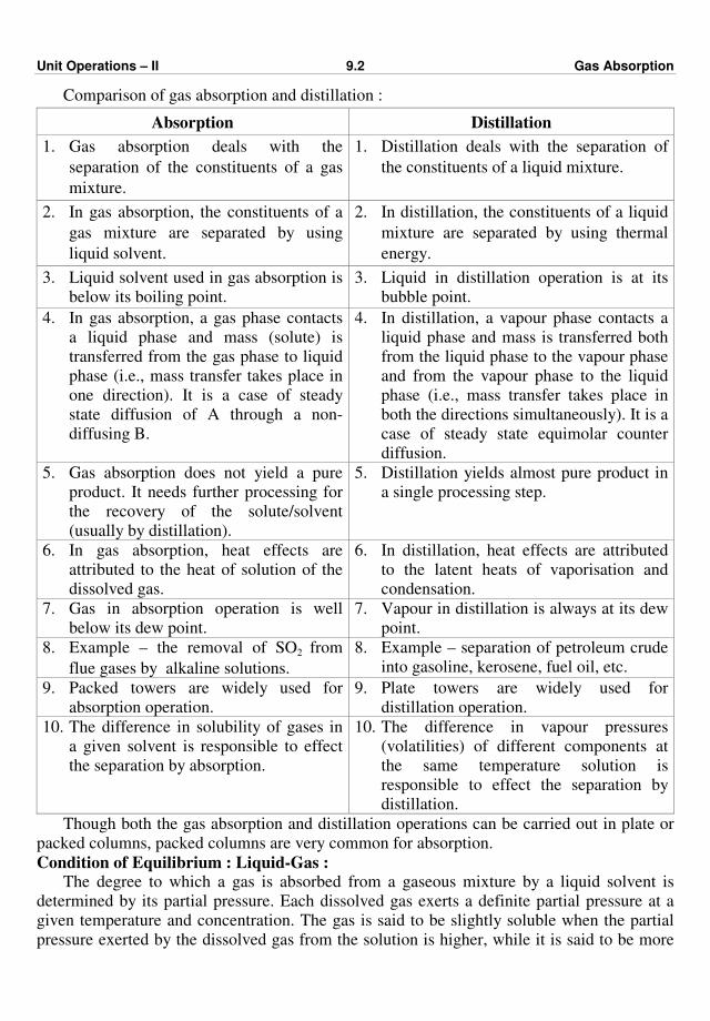
Unit Operations – II 9.2 Gas Absorption
Comparison of gas absorption and distillation :
Absorption Distillation
1. Gas absorption deals with the
separation of the constituents of a gas
mixture.
1. Distillation deals with the separation of
the constituents of a liquid mixture.
2. In gas absorption, the constituents of a
gas mixture are separated by using
liquid solvent.
2. In distillation, the constituents of a liquid
mixture are separated by using thermal
energy.
3. Liquid solvent used in gas absorption is
below its boiling point.
3. Liquid in distillation operation is at its
bubble point.
4. In gas absorption, a gas phase contacts
a liquid phase and mass (solute) is
transferred from the gas phase to liquid
phase (i.e., mass transfer takes place in
one direction). It is a case of steady
state diffusion of A through a non-
diffusing B.
4. In distillation, a vapour phase contacts a
liquid phase and mass is transferred both
from the liquid phase to the vapour phase
and from the vapour phase to the liquid
phase (i.e., mass transfer takes place in
both the directions simultaneously). It is a
case of steady state equimolar counter
diffusion.
5. Gas absorption does not yield a pure
product. It needs further processing for
the recovery of the solute/solvent
(usually by distillation).
5. Distillation yields almost pure product in
a single processing step.
6. In gas absorption, heat effects are
attributed to the heat of solution of the
dissolved gas.
6. In distillation, heat effects are attributed
to the latent heats of vaporisation and
condensation.
7. Gas in absorption operation is well
below its dew point.
7. Vapour in distillation is always at its dew
point.
8. Example – the removal of SO2 from
flue gases by alkaline solutions.
8. Example – separation of petroleum crude
into gasoline, kerosene, fuel oil, etc.
9. Packed towers are widely used for
absorption operation.
9. Plate towers are widely used for
distillation operation.
10. The difference in solubility of gases in
a given solvent is responsible to effect
the separation by absorption.
10. The difference in vapour pressures
(volatilities) of different components at
the same temperature solution is
responsible to effect the separation by
distillation.
Though both the gas absorption and distillation operations can be carried out in plate or
packed columns, packed columns are very common for absorption.
Condition of Equilibrium : Liquid-Gas : The degree to which a gas is absorbed from a gaseous mixture by a liquid solvent is
determined by its partial pressure. Each dissolved gas exerts a definite partial pressure at a
given temperature and concentration. The gas is said to be slightly soluble when the partial
pressure exerted by the dissolved gas from the solution is higher, while it is said to be more
Unit Operations – II 9.3 Gas Absorption
soluble when the partial pressure exerted by the dissolved gas from the solution of given
concentration is lower. Thus, oxygen is slightly soluble, while ammonia is highly soluble in
water. With water as a solvent, ammonia is very soluble gas, sulphur dioxide is moderately
soluble gas and oxygen is slightly soluble gas.
A given quantity of liquid will dissolve any amount of a slightly or more soluble gas
depending upon the partial pressure of the dissolved gas in the gas phase in contact with the
liquid. A slightly soluble (insoluble gas) gas requires a higher partial pressure of the gas in
contact with the liquid to yield the solution of a desired concentration, while a very soluble
gas requires very low partial pressure to give the solution of the same concentration.
Equilibrium condition will be reached when the partial pressure of solute gas in the gas
phase is equal to its partial pressure from the liquid phase. The equilibrium condition thus
fixes the upper limit for operation of an absorption unit.
The solubility of a gas (the concentration of a dissolved gas in the liquid at a given
temperature and pressure) is not substantially affected by the total pressure over the system
but gets influenced by the temperature. Generally, the solubility of a gas in a given solvent
decreases with increase in temperature.
In a majority of cases, the gas absorption results with the evolution of heat and solubility
falls off if provisions are not made to remove the heat evolved. Usually adequate cooling
arrangements are provided to keep the temperature sufficiently low to achieve a good rate of
absorption.
For dilute solutions of most gases, the equilibrium relationship is given by Henry's law :
pA = H · xA … (9.1)
where pA is partial pressure of the solute gas A in the gas phase
xA is mole fraction of the solute gas A in the liquid phase (the
concentration of A in terms of mole fraction)
H is the Henry's law constant.
Please refer to Equilibrium - Chapter 7 for Equilibrium in gas absorption.
Selection criteria for solvent in gas absorption :
While selecting a particular solvent for absorption operation, the following properties of
the solvent are considered :
1. Gas solubility :
The solubility of a solute gas in a solvent should be high, i.e., the solvent should have a
high capacity for dissolving the desired solute gas so that the less amount of the solvent will
be required for a given absorption duty. In general, for good solubility, a solvent of chemical
nature similar to that of the solute to be absorbed must be searched out and used.
The solvent selected should have a high solubility for the solute to be absorbed.
2. Volatility :
As the gas leaving an absorption unit is generally saturated with the solvent, there will be
a loss of the solvent with the gas leaving the unit operation. Hence, to minimise the solvent
loss (in the gas leaving), the solvent should be less volatile, i.e., it should have a low vapour
pressure under given operating conditions.
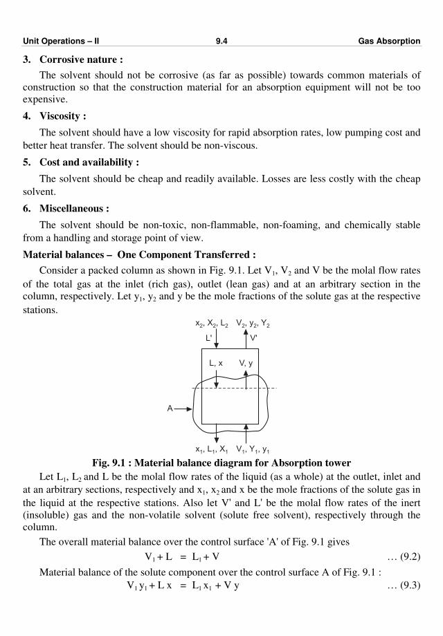
Unit Operations – II 9.4 Gas Absorption
3. Corrosive nature :
The solvent should not be corrosive (as far as possible) towards common materials of
construction so that the construction material for an absorption equipment will not be too
expensive.
4. Viscosity :
The solvent should have a low viscosity for rapid absorption rates, low pumping cost and
better heat transfer. The solvent should be non-viscous.
5. Cost and availability :
The solvent should be cheap and readily available. Losses are less costly with the cheap
solvent.
6. Miscellaneous :
The solvent should be non-toxic, non-flammable, non-foaming, and chemically stable
from a handling and storage point of view.
Material balances – One Component Transferred :
Consider a packed column as shown in Fig. 9.1. Let V1, V2 and V be the molal flow rates
of the total gas at the inlet (rich gas), outlet (lean gas) and at an arbitrary section in the
column, respectively. Let y1, y2 and y be the mole fractions of the solute gas at the respective
stations.
x , X , L2 2 2 V , y , Y2 2 2
L' V'
L, x V, y
A
x , L , X1 1 1 V , Y , y1 1 1 Fig. 9.1 : Material balance diagram for Absorption tower
Let L1, L2 and L be the molal flow rates of the liquid (as a whole) at the outlet, inlet and
at an arbitrary sections, respectively and x1, x2 and x be the mole fractions of the solute gas in
the liquid at the respective stations. Also let V' and L' be the molal flow rates of the inert
(insoluble) gas and the non-volatile solvent (solute free solvent), respectively through the
column.
The overall material balance over the control surface 'A' of Fig. 9.1 gives
V1 + L = L1 + V … (9.2)
Material balance of the solute component over the control surface A of Fig. 9.1 :
V1 y1 + L x = L1 x1 + V y … (9.3)

Unit Operations – II 9.5 Gas Absorption
The overall material balance over the entire column is
V1 + L2 = V2 + L1 … (9.4)
The material balance of the solute over the entire column is
V1 y1 + L2 x2 = L1 x1 + V2 y2 … (9.5)
where y is the mole fraction of the solute in the gas phase
and (1 – y) is the mole fraction of the inert gas in the gas phase
Therefore, V' = V (1 – y) = V1 (1 – y1) = V2 (1 – y2) … (9.6)
Similarly, (1 – x) be the mole fraction of the solute free solvent in the liquid phase.
∴ L' = L (1 – x) = L1 (1 – x1) = L2 (1 – x2) … (9.7)
Equation (9.3) becomes
V'
y1
1 – y1 + L'
x
1 – x = L'
x1
1 – x1 + V'
y
1 – x … (9.8)
∴ V'
y1
1 – y1 –
y
1 – y = L'
x1
1 – x1 –
x
1 – x … (9.9)
Let Y and X be the mole ratio defined as :
Y = y
1 – y
= moles solute per mole of solute-free gas (inert gas)
X = x
1 – x moles solute per mole of solute-free solvent.
(As in 1 mole of a gas mixture, there will be y moles of the solute gas and (1 – y) moles
of the inert gas (insoluble gas).
Equation (9.9) is the equation of the operating line for absorption operation in terms of
mole fraction and is a curve on x - y co-ordinates.
Equation (9.9) in terms of mole ratio is :
V' [Y1 – Y] = L' [X1 – X] … (9.10)
Equation (9.10) is the equation of the operating line for absorption operation. It is a
straight line on x - y co-ordinates with a slope equal to L'/V' and passes through point
(X1, Y1). The line also passes through point (X2, Y2).
Material balance of the solute gas component over the entire tower/column in terms of
L', V' and mole ratios is :
V' [Y1 – Y2] = L' [X1 – X2] … (9.11)
If the solvent used is pure/fresh, x2 = 0 and X2 = 0, then the above equation becomes
V' [Y1 – Y2] = L' (X1) … (9.12)
Minimum Liquid Gas Ratio : Refer to Fig. 9.2.

Unit Operations – II 9.6 Gas Absorption
Consider that the values of the terms V', Y1, Y2 and X2 are fixed by a process requirement
and the value of L' is decreased through the absorption tower. The operating line on X, Y
coordinates passes through the point (X2, Y2) and has a slope equal to L'/V'. As the liquid
flow rate is decreased, the slope of the operating line decreases (operating line shifts toward
the equilibrium curve) and the exist liquid composition (with respect to the solute) increases
from X'1 to X
"1 as indicated by line AC. A reduction in the liquid flow rate reduces the
driving force for mass transfer and absorption becomes more and more difficult. Further
reduction in the liquid flow rate leads to a situation wherein the upper end of the operating
line touches the equilibrium curve as indicated by line AD and the exist liquid composition is
then in equilibrium with the inlet gas. Thus, the driving force for mass transfer becomes zero
at the bottom of the tower, required time of contact for the desired concentration change
becomes infinite, and an infinitely tall tower is required. The value of L'/V' corresponding to
this situation (corresponding to the line AD) represents a minimum liquid-gas ratio. If tower
is to operate practically, the liquid flow rate should be greater than that corresponding to the
minimum L'/V' ratio.
Low values of L'/V' ratio result into taller tower and hence there is an increase in the
fixed cost but the recovery cost of the solute will be low (due to small quantities of liquid).
High values of L'/V' ratio result into small tower due to favourable driving force, and hence,
there is a decrease in the fixed cost but the recovery cost of the solute will be higher.
Therefore, while selecting L'/V' ratio, a balance must be made between the fixed and the
recovery costs. In general, the operating liquid flow rate for the absorber is usually 1.1 to 1.5
times the minimum.
Y
B C DY1
molessolutemolesinertgas
Y2 A
X2
(L'/V
')
Operatingline forminimumL'/V' ratio
Equilibriumcurve
X'1 X''1 X1
Xmolessolutemolessolvent
Fig. 9.2 : Minimum liquid-gas ratio for absorption
Pressure drop in packed columns :
In packed columns operated in a counter current fashion, the liquid fed at the top flows
downward under the influence of gravity/gravitational force and the gas fed at the bottom of
the column is moved upward by a fluid moving machinery such as a blower or fan. So as to
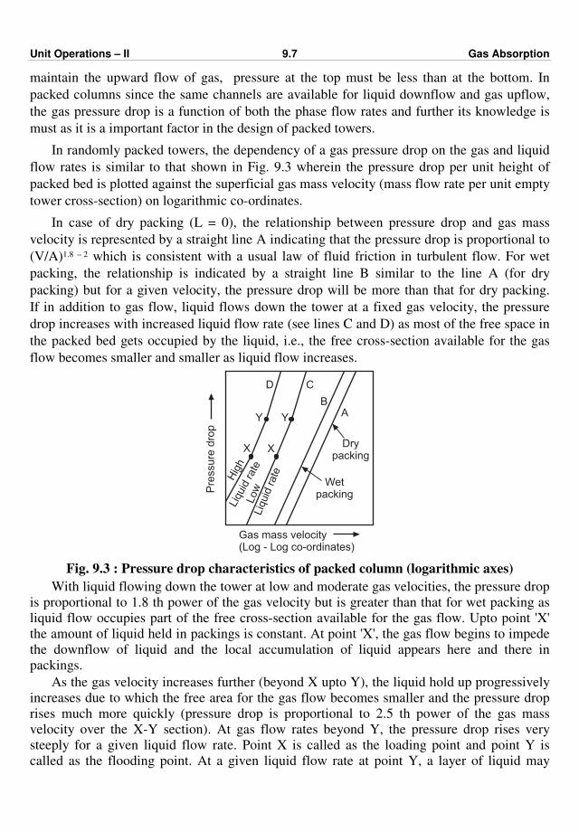
Unit Operations – II 9.7 Gas Absorption
maintain the upward flow of gas, pressure at the top must be less than at the bottom. In
packed columns since the same channels are available for liquid downflow and gas upflow,
the gas pressure drop is a function of both the phase flow rates and further its knowledge is
must as it is a important factor in the design of packed towers.
In randomly packed towers, the dependency of a gas pressure drop on the gas and liquid
flow rates is similar to that shown in Fig. 9.3 wherein the pressure drop per unit height of
packed bed is plotted against the superficial gas mass velocity (mass flow rate per unit empty
tower cross-section) on logarithmic co-ordinates.
In case of dry packing (L = 0), the relationship between pressure drop and gas mass
velocity is represented by a straight line A indicating that the pressure drop is proportional to
(V/A)1.8 – 2 which is consistent with a usual law of fluid friction in turbulent flow. For wet
packing, the relationship is indicated by a straight line B similar to the line A (for dry
packing) but for a given velocity, the pressure drop will be more than that for dry packing.
If in addition to gas flow, liquid flows down the tower at a fixed gas velocity, the pressure
drop increases with increased liquid flow rate (see lines C and D) as most of the free space in
the packed bed gets occupied by the liquid, i.e., the free cross-section available for the gas
flow becomes smaller and smaller as liquid flow increases.
Pre
ssu
re d
rop
Gas mass velocity(Log - Log co-ordinates)
Drypacking
Wetpacking
D C
Y Y
BA
X X
Hig
hLiq
uid
rate
Liq
uid
rate
Low
Fig. 9.3 : Pressure drop characteristics of packed column (logarithmic axes)
With liquid flowing down the tower at low and moderate gas velocities, the pressure drop
is proportional to 1.8 th power of the gas velocity but is greater than that for wet packing as
liquid flow occupies part of the free cross-section available for the gas flow. Upto point 'X'
the amount of liquid held in packings is constant. At point 'X', the gas flow begins to impede
the downflow of liquid and the local accumulation of liquid appears here and there in
packings.
As the gas velocity increases further (beyond X upto Y), the liquid hold up progressively
increases due to which the free area for the gas flow becomes smaller and the pressure drop
rises much more quickly (pressure drop is proportional to 2.5 th power of the gas mass
velocity over the X-Y section). At gas flow rates beyond Y, the pressure drop rises very
steeply for a given liquid flow rate. Point X is called as the loading point and point Y is
called as the flooding point. At a given liquid flow rate at point Y, a layer of liquid may
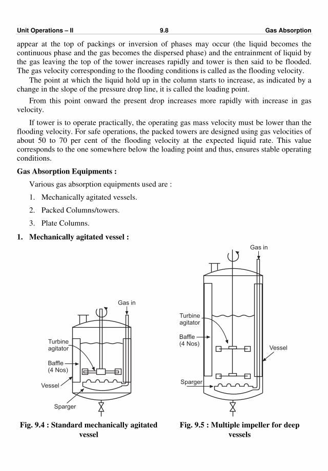
Unit Operations – II 9.8 Gas Absorption
appear at the top of packings or inversion of phases may occur (the liquid becomes the
continuous phase and the gas becomes the dispersed phase) and the entrainment of liquid by
the gas leaving the top of the tower increases rapidly and tower is then said to be flooded.
The gas velocity corresponding to the flooding conditions is called as the flooding velocity.
The point at which the liquid hold up in the column starts to increase, as indicated by a
change in the slope of the pressure drop line, it is called the loading point.
From this point onward the present drop increases more rapidly with increase in gas
velocity.
If tower is to operate practically, the operating gas mass velocity must be lower than the
flooding velocity. For safe operations, the packed towers are designed using gas velocities of
about 50 to 70 per cent of the flooding velocity at the expected liquid rate. This value
corresponds to the one somewhere below the loading point and thus, ensures stable operating
conditions.
Gas Absorption Equipments :
Various gas absorption equipments used are :
1. Mechanically agitated vessels.
2. Packed Columns/towers.
3. Plate Columns.
1. Mechanically agitated vessel :
Gas in
Turbineagitator
Baffle(4 Nos)
Vessel
Sparger
Vessel
Gas in
Turbineagitator
Baffle(4 Nos)
Sparger
Fig. 9.4 : Standard mechanically agitated
vessel
Fig. 9.5 : Multiple impeller for deep
vessels
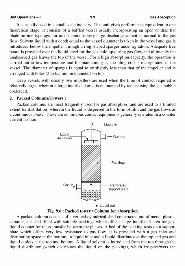
Unit Operations – II 9.9 Gas Absorption
It is usually used in a small scale industry. This unit gives performance equivalent to one
theoretical stage. It consists of a baffled vessel usually incorporating an open or disc flat
blade turbine type agitator as it maintains very large discharge velocities normal to the gas
flow. Solvent liquid with a depth equal to the vessel diameter is taken in the vessel and gas is
introduced below the impeller through a ring shaped sparger under agitation. Adequate free
board is provided over the liquid level for the gas hold up during gas flow and ultimately the
unabsorbed gas leaves the top of the vessel. For a high absorption capacity, the operation is
carried out at low temperature and for maintaining it, a cooling coil is incorporated in the
vessel. The diameter of sparger is equal to or slightly less than that of the impeller and is
arranged with holes (3 to 6.5 mm in diameter) on top.
Deep vessels with usually two impellers are used when the time of contact required is
relatively large, wherein a large interfacial area is maintained by redispersing the gas bubble
coalesced.
2. Packed Columns/Towers :
Packed columns are most frequently used for gas absorption (and are used to a limited
extent for distillation) wherein the liquid is dispersed in the form of film and the gas flows as
a continuous phase. These are continuous contact equipments generally operated in a counter
current fashion.
Liquid out
Liquid in
Gas in
Liquiddistributor Gas out
Packings
Perforatedsupport plate
Fig. 9.6 : Packed tower / Column for absorption
A packed column consists of a vertical cylindrical shell constructed out of metal, plastic,
ceramic, etc. and filled with suitable packings which offer a large interfacial area for gas-
liquid contact for mass transfer between the phases. A bed of the packing rests on a support
plate which offers very low resistance to gas flow. It is provided with a gas inlet and
distributing space at the bottom, a liquid inlet and a liquid distributor at the top and gas and
liquid outlets at the top and bottom. A liquid solvent is introduced from the top through the
liquid distributor (which distributes the liquid on the packing), which irrigates/wets the
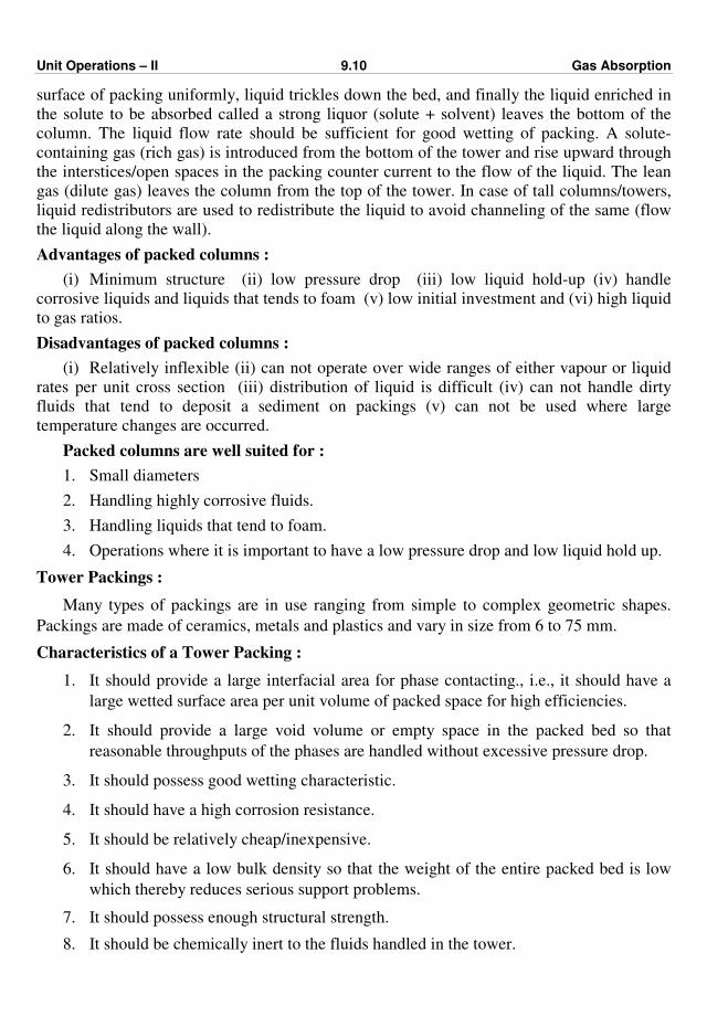
Unit Operations – II 9.10 Gas Absorption
surface of packing uniformly, liquid trickles down the bed, and finally the liquid enriched in
the solute to be absorbed called a strong liquor (solute + solvent) leaves the bottom of the
column. The liquid flow rate should be sufficient for good wetting of packing. A solute-
containing gas (rich gas) is introduced from the bottom of the tower and rise upward through
the interstices/open spaces in the packing counter current to the flow of the liquid. The lean
gas (dilute gas) leaves the column from the top of the tower. In case of tall columns/towers,
liquid redistributors are used to redistribute the liquid to avoid channeling of the same (flow
the liquid along the wall).
Advantages of packed columns :
(i) Minimum structure (ii) low pressure drop (iii) low liquid hold-up (iv) handle
corrosive liquids and liquids that tends to foam (v) low initial investment and (vi) high liquid
to gas ratios.
Disadvantages of packed columns :
(i) Relatively inflexible (ii) can not operate over wide ranges of either vapour or liquid
rates per unit cross section (iii) distribution of liquid is difficult (iv) can not handle dirty
fluids that tend to deposit a sediment on packings (v) can not be used where large
temperature changes are occurred.
Packed columns are well suited for :
1. Small diameters
2. Handling highly corrosive fluids.
3. Handling liquids that tend to foam.
4. Operations where it is important to have a low pressure drop and low liquid hold up.
Tower Packings :
Many types of packings are in use ranging from simple to complex geometric shapes.
Packings are made of ceramics, metals and plastics and vary in size from 6 to 75 mm.
Characteristics of a Tower Packing :
1. It should provide a large interfacial area for phase contacting., i.e., it should have a
large wetted surface area per unit volume of packed space for high efficiencies.
2. It should provide a large void volume or empty space in the packed bed so that
reasonable throughputs of the phases are handled without excessive pressure drop.
3. It should possess good wetting characteristic.
4. It should have a high corrosion resistance.
5. It should be relatively cheap/inexpensive.
6. It should have a low bulk density so that the weight of the entire packed bed is low
which thereby reduces serious support problems.
7. It should possess enough structural strength.
8. It should be chemically inert to the fluids handled in the tower.
Unit Operations – II 9.11 Gas Absorption
Types of packings :
In order to obtain the efficient gas-liquid contact, many different types of packings are
available ranging from simple to complex geometrical shapes but are generally classified as
random packings and regular packings. If the packings are simply dumped into the tower
during installation and fall in a random fashion (the individual pieces are not arranged in any
particular pattern), they are called random packings. The packings arranged in a particular
pattern are called stacked packings.
Pall ring Cross partition ring Intalox saddle
Super intalox packing Intalox saddle
Lessing ring Raschig ring Fig. 9.7 : Tower Packings
In case of randomly packed installations for obtaining the high and uniform voidage and
preventing breakage, a tower is first filled with liquid (usually water) and packings are then
dumped into it. Most common random packings used in industrial towers are Raschig rings,
Pall rings, Hy-pak, Berl saddles, Intalox saddles, Super intalox saddles, etc. As Pall rings,
Unit Operations – II 9.12 Gas Absorption
and Intalox saddles permit a more economical tower design they are replacing older Raschig
rings and Berl saddles. Pall rings are made out of metal or plastic (poly propylene) and have
the same general form as Raschig rings with height equal to diameter, however portions of
the original cylinder wall are cut with the projections bent inward leaving holes in the wall.
They are generally available in sizes ranging from 16 to 50 mm (5/8 to 2 in).
Berl saddles and Intalox saddles are available in range 6 to 50 mm and are formed out of
plastic or ceramics. They provide more gas-liquid contacting area than the Raschig rings.
Raschig rings are hollow cylinders with their length equal to outside diameter and
usually formed out of ceramic, carbon and metal. They are generally available in a size
ranging from 6 to 100 mm
1
4 to 4 in . They are simple in construction and relatively cheap
as compared to other packings. When a single web is added to the inside of the Raschig ring,
the packing is called Lessing ring and when a cross web is added to the Raschig ring, then
the packing formed is called cross partition ring. Added webs provide additional active
surface. They are normally available in a size ranging from 75 to 150 mm (3 to 6 in) and
usually used as stacked packings. Stacked packings offer lower pressure drops for the gas
than random packings for equivalent phase flow rates.
Channeling in Packed Columns : The tendency of the liquid to segregate towards the walls of a packed column and to flow
along the walls (a region of the greatest void space) is termed as channeling, which leads to
low mass transfer efficiencies. Thus, with a good initial liquid distribution in randomly
packed columns, channeling can be minimised by providing a tower diameter to packing size
ratio greater than 8, i.e., the diameter of the tower should be at least eight times the packing
size (or the packing size smaller than at least one-eighth of the tower diameter).
In packed columns, the region of greatest void space is the region near the wall of the
column since the packing material cannot nest tightly with the plane wall as it does with
itself. It is a natural tendency for the fluid to move toward the region of greatest void space
during its flow.
Height Equivalent to an Equilibrium stage (Theoretical Plate) :
The height equivalent to a theoretical plate (HETP) is the height of a section of packing
that will give the same separation as that achieved with one theoretical plate. The HETP is
determined experimentally and is characteristic of each packing. It depends upon the type
and size of the packing, flow rates of fluids and concentration. The height of a packed
column (i.e., the height of packing) required to effect a given degree separation is calculated
by multiplying the number of theoretical plates required to achieve the same degree of
separation by HETP.
Liquid distribution :
For maximum active surface area, the packing should be wetted completely by the
descending liquid and this can be achieved by its proper distribution. For efficient column
operation, uniform distribution of the liquid at the top of the packed bed is essential. A liquid
distributor is a device that spreads the liquid uniformly across the top of the packing. Several
types of liquid distributors used are : (1) Perforated pipe distributor; (2) Orifice-type
distributor; (3) Trough-type distributor; and (4) Weir-riser distributor.

Unit Operations – II 9.13 Gas Absorption
Support Plate :
Orifice type distributorWelding ring support plate
Trough type distributor Support plate
Liquid Liquid
Cap type / Gas injection type
Gas
Gas riser
Perforated pipe distributor Wire mesh support (a) Liquid distributor (b) Support plate for packed towers
Fig. 9.8 : Liquid distributors and support plate
In packed columns, the packing support must be sufficiently strong as it carries the
weight of the entire packed bed and at the same time it must have a large free area for
passage of the gas and liquid phases so as to offer a very low resistance to flow of the phases.
Relative merits of plate and packed towers/columns :
The selection of a particular kind of contactor-plate or packed tower for a given mass
transfer operation, generally rests on the cost and profit considerations but in many cases the
choice can be made on the basis of quantitative analysis of relative merits and demerits of the
plate or packed tower. For selecting the right type of contactor for a given mass transfer duty,
the following merits and demerits should be considered.
1. Plate columns operate over a wide range of liquid flow rates without flooding.
Unit Operations – II 9.14 Gas Absorption
2. Plate columns by repeatedly mixing and separation provide a more positive contact
between fluid phases, whereas packed columns may lead to backmixing or by
passing.
3. Because of the difficulties arising in the dispersion of liquid in a packed tower, a
plate tower is more reliable and needs less safety factors at low liquid to gas mass
velocity ratios.
4. Side streams are very easily taken out from plate towers.
5. For plate towers, design information is generally more readily available and it is
more reliable than it for packed towers.
6. Whenever liquid mixtures containing dispersed solids are to be handled, plate towers
should be preferred as cleaning of the plate is very easy.
7. Whenever intermediate cooling arrangement is required to remove the heat of a
solution or reaction, plate towers are preferred. Cooling coils are easily incorporated
in plate towers.
8. For a given duty, the total weight of a dry plate tower is normally less than the weight
of a packed tower but weight of both towers is approximately the same if the liquid
holdup in the plate tower during the operation is taken into account.
9. For a column diameter more than 1200 mm, packed towers are seldom designed and
for a column diameter less than 600 mm, packings are cheaper than plates.
10. For liquids having tendency to foam, packed towers are usually preferred.
11. High values of liquid-gas ratio are best handled in packed towers.
12. Liquid hold-up is considerably low in packed towers so they are used in cases where
liquid deterioration might occur with high temperatures (i.e., used for handling heat-
sensitive liquids).
13. The pressure drop through a packed tower is usually low which makes the packed
tower particularly desirable for vacuum distillation operations.
14. Packed towers may be more economical than plate towers when highly corrosive
fluids are to be handled because of corrosion resistant ceramic/plastic packings.
15. Plate towers are often preferred when large temperature changes are involved, as in
distillation, thermal expansion or contraction of the equipment component may crush
the packing.
Packed columns and plate columns are the commonly used equipments for gas-liquid
operations such as distillation and gas absorption. They are also used for liquid extraction.
Comparison of packed column and plate column :
Packed columns are differential contactors wherein mass transfer occurs throughout the
length of the contactor and equilibrium is not reached at any point between the phases in
contact, whereas plate columns are stagewise contactors wherein mass transfer occurs
intermittently/stagewise and equilibrium is established between the phases at a number of
discrete stages. In packed columns, packings are used as gas-liquid contacting devices,
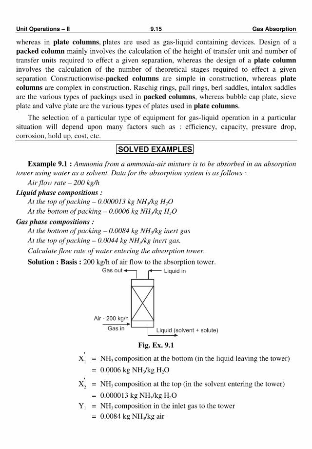
Unit Operations – II 9.15 Gas Absorption
whereas in plate columns, plates are used as gas-liquid containing devices. Design of a
packed column mainly involves the calculation of the height of transfer unit and number of
transfer units required to effect a given separation, whereas the design of a plate column
involves the calculation of the number of theoretical stages required to effect a given
separation Constructionwise-packed columns are simple in construction, whereas plate
columns are complex in construction. Raschig rings, pall rings, berl saddles, intalox saddles
are the various types of packings used in packed columns, whereas bubble cap plate, sieve
plate and valve plate are the various types of plates used in plate columns.
The selection of a particular type of equipment for gas-liquid operation in a particular
situation will depend upon many factors such as : efficiency, capacity, pressure drop,
corrosion, hold up, cost, etc.
SOLVED EXAMPLES
Example 9.1 : Ammonia from a ammonia-air mixture is to be absorbed in an absorption
tower using water as a solvent. Data for the absorption system is as follows :
Air flow rate – 200 kg/h
Liquid phase compositions :
At the top of packing – 0.000013 kg NH3/kg H2O
At the bottom of packing – 0.0006 kg NH3/kg H2O
Gas phase compositions :
At the bottom of packing – 0.0084 kg NH3/kg inert gas
At the top of packing – 0.0044 kg NH3/kg inert gas.
Calculate flow rate of water entering the absorption tower.
Solution : Basis : 200 kg/h of air flow to the absorption tower.
Air - 200 kg/h
Gas in Liquid (solvent + solute)
Gas out Liquid in
Fig. Ex. 9.1
X'1 = NH3 composition at the bottom (in the liquid leaving the tower)
= 0.0006 kg NH3/kg H2O
X'2 = NH3 composition at the top (in the solvent entering the tower)
= 0.000013 kg NH3/kg H2O
Y1 = NH3 composition in the inlet gas to the tower
= 0.0084 kg NH3/kg air
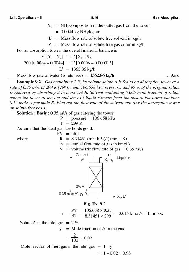
Unit Operations – II 9.16 Gas Absorption
Y2 = NH3 composition in the outlet gas from the tower
= 0.0044 kg NH3/kg air
L' = Mass flow rate of solute free solvent in kg/h
V' = Mass flow rate of solute free gas or air in kg/h
For an absorption tower, the overall material balance is
V' [Y1 – Y2] = L' [X1 – X2]
200 [0.0084 – 0.0044] = L' [0.0006 – 0.000013]
L' = 1362.86 kg/h
Mass flow rate of water (solute free) = 1362.86 kg/h … Ans.
Example 9.2 : Gas containing 2 % by volume solute A is fed to an absorption tower at a
rate of 0.35 m3/s at 299 K (26o C) and 106.658 kPa pressure, and 95 % of the original solute
is removed by absorbing it in a solvent B. Solvent containing 0.005 mole fraction of solute
enters the tower at the top and the exit liquid streams from the absorption tower contains
0.12 mole A per mole B. Find out the flow rate of the solvent entering the absorption tower
on solute-free basis.
Solution : Basis : 0.35 m3/s of gas entering the tower.
P = pressure = 106.658 kPa
T = 299 K
Assume that the ideal gas law holds good.
PV = nRT
where R = 8.31451 (m3 · kPa)/ (kmol · K)
n = molal flow rate of gas in kmol/s
V = volumetric flow rate of gas = 0.35 m3/s
2% A
0.35 m /s V', y , Y3
1 1X , L'1
Gas outLiquid in
X , x2 2
L'
V'
Fig. Ex. 9.2
n = PV
RT =
106.658 × 0.35
8.31451 × 299 = 0.015 kmol/s = 15 mol/s
Solute A in the inlet gas = 2 %
y1 = Mole fraction of A in the gas
= 2
100 = 0.02
Mole fraction of inert gas in the inlet gas = 1 – y1
= 1 – 0.02 = 0.98
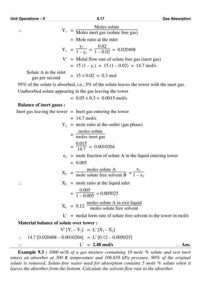
Unit Operations – II 9.17 Gas Absorption
∴ Y1 = Moles solute
Moles inert gas (solute free gas)
= Mole ratio at the inlet
Y1 = y1
1 – y1 =
0.02
1 – 0.02 = 0.020408
V' = Molal flow rate of solute free gas (inert gas)
= 15 (1 – y1) = 15 (1 – 0.02) = 14.7 mol/s
Solute A in the inlet
gas per second = 15 × 0.02 = 0.3 mol
95% of the solute is absorbed, i.e., 5% of the solute leaves the tower with the inert gas.
Unabsorbed solute appearing in the gas leaving the tower
= 0.05 × 0.3 = 0.0015 mol/s
Balance of inert gases :
Inert gas leaving the tower = Inert gas entering the tower
= 14.7 mol/s
Y2 = mole ratio at the outlet (gas phase)
= moles solute
moles inert gas
= 0.015
14.7 = 0.0010204
x2 = mole fraction of solute A in the liquid entering tower
= 0.005
X2 = moles solute A
mole solute free solvent B =
x2
1 – x2
∴ X2 = mole ratio at the liquid inlet
= 0.005
1 – 0.005 = 0.005025
X1 = 0.12 moles solute A in exit liquid
moles solute free solvent
L' = molal form rate of solute free solvent to the tower in mol/s
Material balance of solute over tower :
V' [Y1 – Y2] = L' [X1 – X2]
∴ 14.7 [0.020408 – 0.0010204] = L' [0.12 – 0.005025]
∴ L' = 2.48 mol/s … Ans.
Example 9.3 : 1000 m3/h of a gas mixture containing 10 mole % solute and rest inert
enters an absorber at 300 K temperature and 106.658 kPa pressure. 90% of the original
solute is removed. Solute-free water used for absorption contains 5 mole % solute when it
leaves the absorber from the bottom. Calculate the solvent flow rate to the absorber.
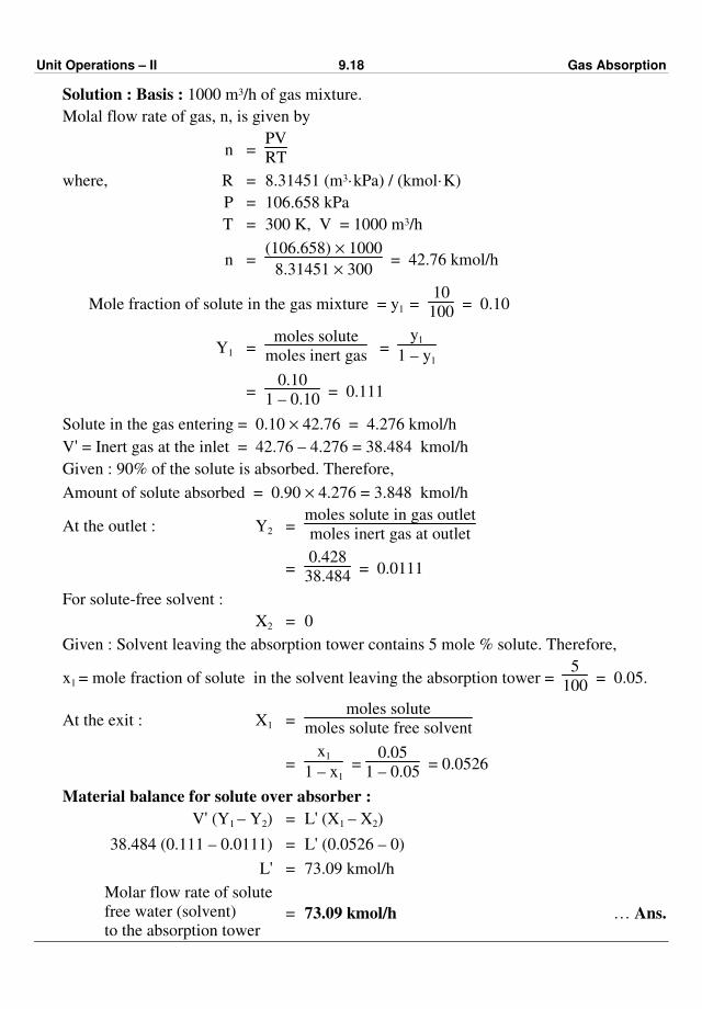
Unit Operations – II 9.18 Gas Absorption
Solution : Basis : 1000 m3/h of gas mixture.
Molal flow rate of gas, n, is given by
n = PV
RT
where, R = 8.31451 (m3·kPa) / (kmol·K)
P = 106.658 kPa
T = 300 K, V = 1000 m3/h
n = (106.658) × 1000
8.31451 × 300 = 42.76 kmol/h
Mole fraction of solute in the gas mixture = y1 = 10
100 = 0.10
Y1 = moles solute
moles inert gas =
y1
1 – y1
= 0.10
1 – 0.10 = 0.111
Solute in the gas entering = 0.10 × 42.76 = 4.276 kmol/h
V' = Inert gas at the inlet = 42.76 – 4.276 = 38.484 kmol/h
Given : 90% of the solute is absorbed. Therefore,
Amount of solute absorbed = 0.90 × 4.276 = 3.848 kmol/h
At the outlet : Y2 = moles solute in gas outlet
moles inert gas at outlet
= 0.428
38.484 = 0.0111
For solute-free solvent :
X2 = 0
Given : Solvent leaving the absorption tower contains 5 mole % solute. Therefore,
x1 = mole fraction of solute in the solvent leaving the absorption tower = 5
100 = 0.05.
At the exit : X1 = moles solute
moles solute free solvent
= x1
1 – x1 =
0.05
1 – 0.05 = 0.0526
Material balance for solute over absorber :
V' (Y1 – Y2) = L' (X1 – X2)
38.484 (0.111 – 0.0111) = L' (0.0526 – 0)
L' = 73.09 kmol/h
Molar flow rate of solute
free water (solvent)
to the absorption tower = 73.09 kmol/h … Ans.

Unit Operations – II 9.19 Gas Absorption
Example 9.4 : Benzene is to be recovered from cool gas by scrubbing it with wash oil as
an absorbent. The coal gas contains 2 % by volume of benzene and is to be fed at a rate of
855 m3/h and 95 % removal of benzene is required. The operating temperature and pressure
are 299.7 K (26.7o C) and 106.658 kPa. The wash oil has an average molecular weight of
260 and contains 0.005 mole fraction benzene as it enters the absorber. Calculate the
minimum circulation rate of the wash oil. The equilibrium relationship at the given
conditions is given by
Y
1 + Y = 0.125
X
1 + X
where, Y – moles benzene/mole dry coal gas.
X – moles benzene/mole benzene free wash oil.
Solution : Basis : 855 m3/h of coal gas.
Assuming ideal gas behaviour, the molal flow rate of coal gas is given by
n = PV
RT
where V is the volumetric flow rate of coal gas.
P = 106.658 kPa,
T = 299.7 K, V = 855 m3/h
R = 8.31451 m3·kPa
kmol·K
n = (106.658) × 855
8.31451 × 299.7
= 36.59 kmol/h
Molal flow rate of the gas at the inlet = V1 = n = 36.59 kmol/h
y1 = mole fraction of benzene in the coal gas
= 2/100 = 0.02
V' = V1 (1 – y1)
= 36.59 (1 – 0.02) = 35.86 kmol/h
Molal flow rate of benzene-free coal gas = 35.86 kmol/h
At the inlet : Y1 = moles benzene
moles dry coal gas
= y1
1 – y1 =
0.02
1 – 0.02
= 0.0204 kmol benzene/kmol benzene-free gas
95% of benzene is removed by absorption.
At the outlet : Y2 = (1 – 0.95) Y1
= 0.05 Y1 = 0.05 × 0.0204
= 0.00102 moles benzene
moles benzene free gas
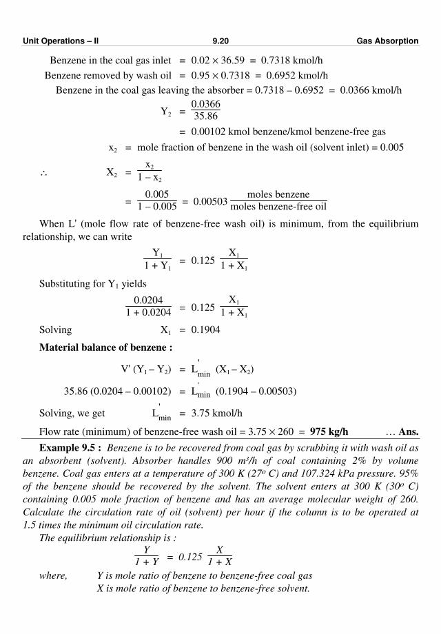
Unit Operations – II 9.20 Gas Absorption
Benzene in the coal gas inlet = 0.02 × 36.59 = 0.7318 kmol/h
Benzene removed by wash oil = 0.95 × 0.7318 = 0.6952 kmol/h
Benzene in the coal gas leaving the absorber = 0.7318 – 0.6952 = 0.0366 kmol/h
Y2 = 0.0366
35.86
= 0.00102 kmol benzene/kmol benzene-free gas
x2 = mole fraction of benzene in the wash oil (solvent inlet) = 0.005
∴ X2 = x2
1 – x2
= 0.005
1 – 0.005 = 0.00503
moles benzene
moles benzene-free oil
When L' (mole flow rate of benzene-free wash oil) is minimum, from the equilibrium
relationship, we can write
Y1
1 + Y1 = 0.125
X1
1 + X1
Substituting for Y1 yields
0.0204
1 + 0.0204 = 0.125
X1
1 + X1
Solving X1 = 0.1904
Material balance of benzene :
V' (Y1 – Y2) = L'min
(X1 – X2)
35.86 (0.0204 – 0.00102) = L'
min (0.1904 – 0.00503)
Solving, we get L'min
= 3.75 kmol/h
Flow rate (minimum) of benzene-free wash oil = 3.75 × 260 = 975 kg/h … Ans.
Example 9.5 : Benzene is to be recovered from coal gas by scrubbing it with wash oil as
an absorbent (solvent). Absorber handles 900 m3/h of coal containing 2% by volume
benzene. Coal gas enters at a temperature of 300 K (27o C) and 107.324 kPa pressure. 95%
of the benzene should be recovered by the solvent. The solvent enters at 300 K (30o C)
containing 0.005 mole fraction of benzene and has an average molecular weight of 260.
Calculate the circulation rate of oil (solvent) per hour if the column is to be operated at
1.5 times the minimum oil circulation rate.
The equilibrium relationship is :
Y
1 + Y = 0.125
X
1 + X
where, Y is mole ratio of benzene to benzene-free coal gas
X is mole ratio of benzene to benzene-free solvent.
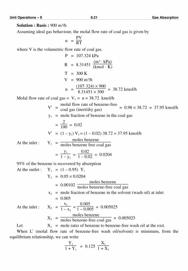
Unit Operations – II 9.21 Gas Absorption
Solution : Basis : 900 m3/h
Assuming ideal gas behaviour, the molal flow rate of coal gas is given by
n = PV
RT
where V is the volumetric flow rate of coal gas.
P = 107.324 kPa
R = 8.31451 (m3 · kPa)
(kmol · K)
T = 300 K
V = 900 m3/h
n = (107·324) × 900
8.31451 × 300 = 38.72 kmol/h
Molal flow rate of coal gas = V1 = n = 38.72 kmol/h
V' = molal flow rate of benzene-free
coal gas (inert/dry gas) = 0.98 × 38.72 = 37.95 kmol/h
y1 = mole fraction of benzene in the coal gas
= 2
100 = 0.02
V' = (1 – y1) V1 = (1 – 0.02) 38.72 = 37.95 kmol/h
At the inlet : Y1 = moles benzene
moles benzene free coal gas
= y1
1 – y1 =
0.02
1 – 0.02 = 0.0204
95% of the benzene is recovered by absorption
At the outlet : Y2 = (1 – 0.95) Y1
Y2 = 0.05 × 0.0204
= 0.00102 moles benzene
moles benzene-free coal gas
x2 = mole fraction of benzene in the solvent (wash oil) at inlet
= 0.005
At the inlet : X2 = x2
1 – x2 =
0.005
1 – 0.005 = 0.005025
X2 = moles benzene
moles benzene-free coal gas = 0.005025
Let X1 = mole ratio of benzene to benzene-free wash oil at the exit.
When L' (molal flow rate of benzene-free wash oil/solvent) is minimum, from the
equilibrium relationship, we can write
Y1
1 + Y1 = 0.125
X1
1 + X1
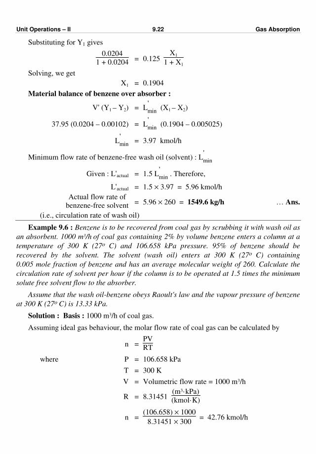
Unit Operations – II 9.22 Gas Absorption
Substituting for Y1 gives
0.0204
1 + 0.0204 = 0.125
X1
1 + X1
Solving, we get
X1 = 0.1904
Material balance of benzene over absorber :
V' (Y1 – Y2) = L'min
(X1 – X2)
37.95 (0.0204 – 0.00102) = L'min
(0.1904 – 0.005025)
L'min
= 3.97 kmol/h
Minimum flow rate of benzene-free wash oil (solvent) : L'min
Given : L'actual = 1.5 L'min
. Therefore,
L'actual = 1.5 × 3.97 = 5.96 kmol/h
Actual flow rate of
benzene-free solvent = 5.96 × 260 = 1549.6 kg/h … Ans.
(i.e., circulation rate of wash oil)
Example 9.6 : Benzene is to be recovered from coal gas by scrubbing it with wash oil as
an absorbent. 1000 m3/h of coal gas containing 2% by volume benzene enters a column at a
temperature of 300 K (27o C) and 106.658 kPa pressure. 95% of benzene should be
recovered by the solvent. The solvent (wash oil) enters at 300 K (27o C) containing
0.005 mole fraction of benzene and has an average molecular weight of 260. Calculate the
circulation rate of solvent per hour if the column is to be operated at 1.5 times the minimum
solute free solvent flow to the absorber.
Assume that the wash oil-benzene obeys Raoult's law and the vapour pressure of benzene
at 300 K (27o C) is 13.33 kPa.
Solution : Basis : 1000 m3/h of coal gas.
Assuming ideal gas behaviour, the molar flow rate of coal gas can be calculated by
n = PV
RT
where P = 106.658 kPa
T = 300 K
V = Volumetric flow rate = 1000 m3/h
R = 8.31451 (m3·kPa)
(kmol·K)
n = (106.658) × 1000
8.31451 × 300 = 42.76 kmol/h
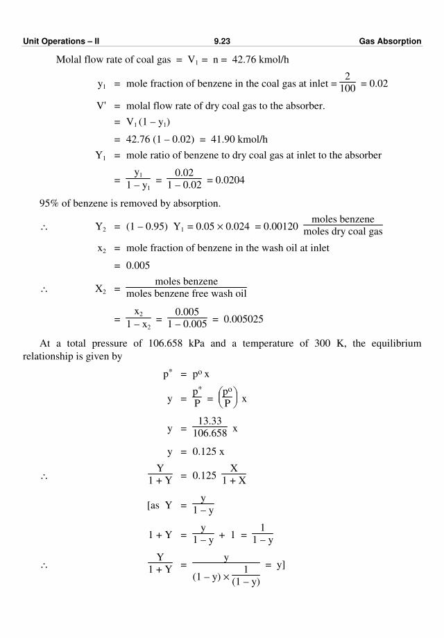
Unit Operations – II 9.23 Gas Absorption
Molal flow rate of coal gas = V1 = n = 42.76 kmol/h
y1 = mole fraction of benzene in the coal gas at inlet = 2
100 = 0.02
V' = molal flow rate of dry coal gas to the absorber.
= V1 (1 – y1)
= 42.76 (1 – 0.02) = 41.90 kmol/h
Y1 = mole ratio of benzene to dry coal gas at inlet to the absorber
= y1
1 – y1 =
0.02
1 – 0.02 = 0.0204
95% of benzene is removed by absorption.
∴ Y2 = (1 – 0.95) Y1 = 0.05 × 0.024 = 0.00120 moles benzene
moles dry coal gas
x2 = mole fraction of benzene in the wash oil at inlet
= 0.005
∴ X2 = moles benzene
moles benzene free wash oil
= x2
1 – x2 =
0.005
1 – 0.005 = 0.005025
At a total pressure of 106.658 kPa and a temperature of 300 K, the equilibrium
relationship is given by
p* = po x
y = p*
P =
po
P x
y = 13.33
106.658 x
y = 0.125 x
∴ Y
1 + Y = 0.125
X
1 + X
[as Y = y
1 – y
1 + Y = y
1 – y + 1 =
1
1 – y
∴ Y
1 + Y =
y
(1 – y) × 1
(1 – y)
= y]
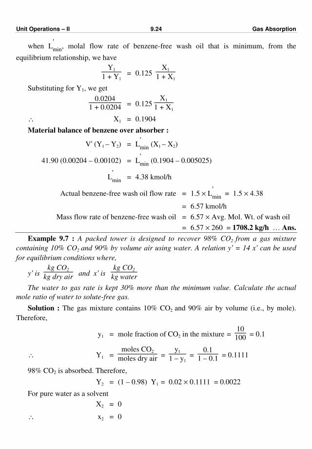
Unit Operations – II 9.24 Gas Absorption
when L'min
, molal flow rate of benzene-free wash oil that is minimum, from the
equilibrium relationship, we have
Y1
1 + Y1 = 0.125
X1
1 + X1
Substituting for Y1, we get
0.0204
1 + 0.0204 = 0.125
X1
1 + X1
∴ X1 = 0.1904
Material balance of benzene over absorber :
V' (Y1 – Y2) = L'min
(X1 – X2)
41.90 (0.00204 – 0.00102) = L'min
(0.1904 – 0.005025)
L'min
= 4.38 kmol/h
Actual benzene-free wash oil flow rate = 1.5 × L'min
= 1.5 × 4.38
= 6.57 kmol/h
Mass flow rate of benzene-free wash oil = 6.57 × Avg. Mol. Wt. of wash oil
= 6.57 × 260 = 1708.2 kg/h … Ans.
Example 9.7 : A packed tower is designed to recover 98% CO2 from a gas mixture
containing 10% CO2 and 90% by volume air using water. A relation y' = 14 x' can be used
for equilibrium conditions where,
y' is kg CO2
kg dry air and x' is
kg CO2
kg water
The water to gas rate is kept 30% more than the minimum value. Calculate the actual
mole ratio of water to solute-free gas.
Solution : The gas mixture contains 10% CO2 and 90% air by volume (i.e., by mole).
Therefore,
y1 = mole fraction of CO2 in the mixture = 10
100 = 0.1
∴ Y1 = moles CO2
moles dry air =
y1
1 – y1 =
0.1
1 – 0.1 = 0.1111
98% CO2 is absorbed. Therefore,
Y2 = (1 – 0.98) Y1 = 0.02 × 0.1111 = 0.0022
For pure water as a solvent
X2 = 0
∴ x2 = 0
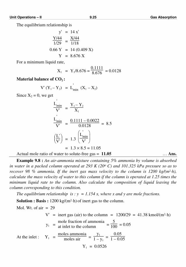
Unit Operations – II 9.25 Gas Absorption
The equilibrium relationship is
y' = 14 x'
Y/44
1/29 =
X/44
1/18
0.66 Y = 14 (0.409 X)
Y = 8.676 X
For a minimum liquid rate,
X1 = Y1/8.676 = 0.1111
8.676 = 0.0128
Material balance of CO2 :
V' (Y1 – Y2) = L'min
(X1 – X2)
Since X2 = 0, we get
L
'min
V' =
Y1 – Y2
X1
L
'min
V' =
0.1111 – 0.0022
0.0128 = 8.5
L'
V' = 1.3
L
'min
V'
= 1.3 × 8.5 = 11.05
Actual mole ratio of water to solute-free gas = 11.05 … Ans.
Example 9.8 : An air-ammonia mixture containing 5% ammonia by volume is absorbed
in water in a packed column operated at 293 K (20o C) and 101.325 kPa pressure so as to
recover 98 % ammonia. If the inert gas mass velocity to the column is 1200 kg/(m2·h),
calculate the mass velocity of water to this column if the column is operated at 1.25 times the
minimum liquid rate to the column. Also calculate the composition of liquid leaving the
column corresponding to this condition.
The equilibrium relationship is : y = 1.154 x, where x and y are mole fractions.
Solution : Basis : 1200 kg/(m2·h) of inert gas to the column.
Mol. Wt. of air = 29
V' = inert gas (air) to the column = 1200/29 = 41.38 kmol/(m2·h)
y1 = mole fraction of ammonia
at inlet to the column = 5
100 = 0.05
At the inlet : Y1 = moles ammonia
moles air =
y1
1 – y1 =
0.05
1 – 0.05
Y1 = 0.0526

Unit Operations – II 9.26 Gas Absorption
98% of ammonia is absorbed. Therefore,
At the outlet : Y2 = moles ammonia
moles air = (1 – 0.98) Y1
= (1 – 0.98) × 0.0526 = 0.001
The equilibrium relationship is
y = 1.154 x
∴ Y
1 + Y = 1.154
X
1 + X
At inlet to the column since water is pure, X2 = 0
At minimum liquid rate :
Y1
1 + Y1 = 1.154
X1
1 + X1
Substituting for Y1 gives
0.0526
1 + 0.0526 = 1.154
X1
1 + X1
X1 = 0.0453
Material balance of ammonia over column :
V' (Y1 – Y2) = L'min
(X1 – X2)
41.38 (0.0526 – 0.001) = L'min
(0.0453 – 0)
∴ L'min
= 41.73 kmol/(m2·h)
L'actual
= 1.25 L'min
= 1.25 × 41.73 = 58.9 kmol/(m2·h)
Actual mass velocity of water to the column
= 58.9 × 18 = 938.92 kg/(m2·h)
Let X'1 be the liquid composition corresponding to this condition.
Hence, 41.38 (0.0526 – 0.001) = 58.9 X'1
Solving X'1 = 0.0363
Composition of liquid leaving the column in terms of mole ratio = 0.0363 ………… Ans.

Unit Operations – II 9.27 Gas Absorption
Example 9.9 : A mixture of acetone vapour and air containing 5% acetone by volume is
to be freed of its acetone content by scrubbing it with water in an absorber. The flow rate of
the gas mixture 700 m3/h of acetone-free air measured at N.T.P. and water flow rate is
1500 kg/h. The absorber operates at an average temperature of 293 K (20 oC) and a
pressure of 101 kPa. 98% of the acetone is absorbed.
The equilibrium relationship for the acetone vapour-water system is : – Y* = 1.68 X.
where Y* = kg mole acetone/kg mole dry air
X = kg mole acetone/kg mole water.
Calculate the quantity of acetone absorbed per hour and the mean driving force for
absorption.
Hint : ∆Ylm = ∆Y1 – ∆Y2
ln (∆Y1/∆Y2)
∆Y1 and ∆Y2 are the driving forces at the top and bottom of the tower. ∆Y = Y – Y*
Solution : Flow rate of acetone-free air
= 700 m3/h N.T.P.
= 700/22.4 = 31.25 kmol/h
[Since 1 kmol of an ideal gas occupies a volume of 22.4 m3]
Flow rate of acetone-free water
= 1500 kg/h
= 1500/18 = 83.33 kmol/h
The mole fraction of acetone in the mixture is
y1 = 5/100 = 0.05
Y1 = y1/(1 – y1) = 0.05
1 – 0.05 = 0.0526
Given : 98% of the acetone is scrubbed. Therefore, we can write
Y2 = (1 – 0.98) Y1 = 0.02 Y1 = 0.02 × 0.0526
Y2 = 0.00105
Water entering the absorber is pure and therefore,
X2 = 0.0
Let us obtain X1.
Solute material balance over absorber :
V' (Y1 – Y2) = L' (X1 – X2)
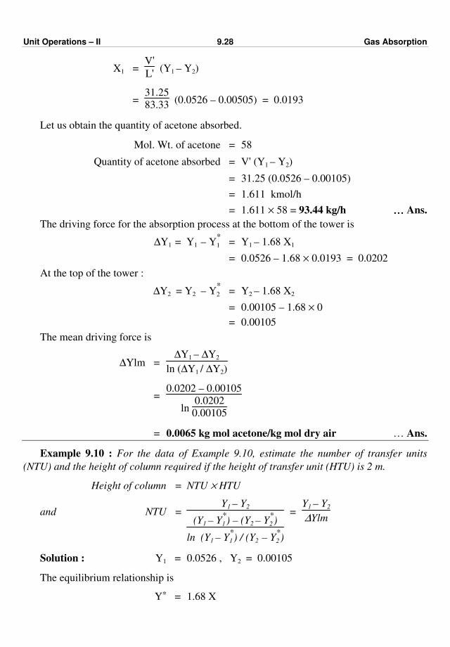
Unit Operations – II 9.28 Gas Absorption
X1 = V'
L' (Y1 – Y2)
= 31.25
83.33 (0.0526 – 0.00505) = 0.0193
Let us obtain the quantity of acetone absorbed.
Mol. Wt. of acetone = 58
Quantity of acetone absorbed = V' (Y1 – Y2)
= 31.25 (0.0526 – 0.00105)
= 1.611 kmol/h
= 1.611 × 58 = 93.44 kg/h ………… Ans.
The driving force for the absorption process at the bottom of the tower is
∆Y1 = Y1 – Y*1 = Y1 – 1.68 X1
= 0.0526 – 1.68 × 0.0193 = 0.0202
At the top of the tower :
∆Y2 = Y2 – Y*2 = Y2 – 1.68 X2
= 0.00105 – 1.68 × 0
= 0.00105
The mean driving force is
∆Ylm = ∆Y1 – ∆Y2
ln (∆Y1 / ∆Y2)
= 0.0202 – 0.00105
ln 0.0202
0.00105
= 0.0065 kg mol acetone/kg mol dry air … Ans.
Example 9.10 : For the data of Example 9.10, estimate the number of transfer units
(NTU) and the height of column required if the height of transfer unit (HTU) is 2 m.
Height of column = NTU × HTU
and NTU = Y1 – Y2
(Y1 – Y*
1) – (Y2 – Y*
2)
ln (Y1 – Y*
1) / (Y2 – Y*
2)
= Y1 – Y2
∆Ylm
Solution : Y1 = 0.0526 , Y2 = 0.00105
The equilibrium relationship is
Y* = 1.68 X
Unit Operations – II 9.29 Gas Absorption
∴ Y*1 = 1.68 X1 = 1.68 × 0.0193 = 0.0324
Y*2 = 1.68 X2 = 1.68 × 0 = 0.0
NTU = (0.0526 – 0.00105)
(0.0526 – 0.0324) – (0.00105 – 0)
ln (0.0526 – 0.0324) / (0.00105)
= 7.95 ≈ 8
Height of packed column = NTU × HTU = 8 × 2 = 16 m … Ans.
EXERCISES
1. Fill in the blanks :
(a) In gas absorption, mass transfer takes place from the ...... phase to the liquid phase.
Ans. gas
(b) ....... used for gas absorption should be less volatile to avoid its loss in a lean gas.
Ans. Solvent
(c) ............. are continuous gas-liquid contactors and ................. are stage-wise
contactors. Ans. Packed columns, plate columns
(d) Operating velocity in packed columns should be 50 to 70% of the .......... velocity.
Ans. flooding
(e) Packing size should not be more than 1/8th of the column ............. Ans. diameter
(f) Absorption of NO2 in water to produce nitric acid is an example of absorption with
............ Ans. chemical reaction.
(g) The tendency of the liquid to segregate towards the walls and to flow along the
walls is termed as ................ Ans. channeling
2. Define gas absorption. What for it is carried out industrially ? Give suitable
examples.
3. What factors should be considered while selecting solvent for gas absorption ?
4. State the desirable characteristics of packings.
5. List various types of packings used in industry and state their materials of
construction.
6. Explain briefly the hydrodynamics / press drop characteristics of a packed column.
7. Compare plate and packed columns for merits and demerits.
8. Draw a neat sketch of packed column and write its construction and functioning.
9. What do you mean by HETP ? State the factors on which HETP depends.
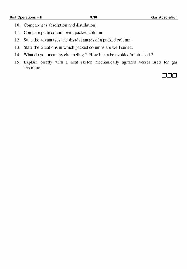
Unit Operations – II 9.30 Gas Absorption
10. Compare gas absorption and distillation.
11. Compare plate column with packed column.
12. State the advantages and disadvantages of a packed column.
13. State the situations in which packed columns are well suited.
14. What do you mean by channeling ? How it can be avoided/minimised ?
15. Explain briefly with a neat sketch mechanically agitated vessel used for gas
absorption.
ppp

(10.1)
CHAPTER TEN
LIQUID-LIQUID EXTRACTION
The techniques of removing one component from a solid or liquid by means of a liquid
solvent fall into two categories, the first one is called as leaching or solid extraction and the
second as liquid extraction. Leaching is used to dissolve soluble matter from its mixture with
an insoluble solid (Leaching is an operation in which a particular component of the solid is
leached out with the help of a solvent), whereas liquid extraction is used to separate two
miscible liquids using a solvent which preferentially dissolves one of them. In this chapter,
our discussion is restricted to liquid extraction – the extraction of the liquid phase with a
solvent.
When a mixture of liquids is not easily separable by distillation, i.e., when the separation
by distillation is ineffective or very difficult, liquid extraction is used. Close boiling mixtures
or substances that cannot withstand the temperature of distillation, even under vacuum
[i.e., substances that are thermally unstable (heat sensitive)] may often be separated by
extraction. In this operation, a solvent is added to the liquid-mixture. As a result, two
immiscible layers are formed, both containing varying amounts of different components. The
isolated layers are then separated using density difference as extract phase and raffinate
phase. For the recovery of the solvent for re-use, extraction is followed often by distillation
or evaporation.
Liquid-liquid extraction (liquid extraction) refers to an operation in which the
constituents of a liquid mixture are separated by contacting it with a suitable insoluble liquid
solvent, which preferentially dissolves one or more constituents. This operation is sometimes
also termed as solvent extraction. Extraction utilises the differences in solubility of
constituents/components to effect a separation. In this operation, a solute in a liquid solution
is removed by contacting the solution with another liquid solvent. The solvent is relatively
immiscible with the solution. In liquid extraction, the feed solution to be handled represents
one phase and the solvent to be used to effect separation represents the second phase. In this
operation, the two immiscible phases in contact are both liquid and so is a liquid-liquid
operation. The mass transfer of the solute (liquid) takes place from the feed solution to the
solvent phase.
Distillation and extraction both are used for separation of the constituents of a liquid
mixture based on relative merits/demerits of the individual methods.

Unit Operations – II 10.2 Liquid-Liquid Extraction
Difference between distillation and extraction.
Distillation Extraction
1. Distillation/fractionation is an operation
in which the constituents of a liquid
mixture are separated by using thermal
energy.
1. Extraction is an operation in which the
constituents of a liquid mixture are
separated by using an insoluble liquid
solvent.
2. Distillation utilises the difference in
vapour pressures of different
components at the same temperature to
effect a separation.
2. Extraction utilises the differences in
solubility of different components to
effect a separation.
3. In distillation, relative volatility is used
as a measure of the degree of separation.
3. In extraction, selectivity is used as a
measure of the degree of separation.
4. In distillation, a new phase is created by
addition of heat.
4. In extraction, a new insoluble liquid
phase is created by addition of solvent to
the original mixture.
5. In distillation, mixing and separation of
phases is easy and rapid.
5. In extraction, phases are hard to mix and
harder to separate.
6. Distillation/fractionation gives almost
pure products.
6. Extraction itself does not give pure
products and needs further processing.
7. It does not offer more flexibility in the
choice of operating conditions.
7. It does offer more flexibility in the
choice of operating conditions.
8. It requires thermal energy. 8. It requires mechanical energy (for
mixing and separation).
9. It needs heating and cooling provisions. 9. It does not need heating and cooling
provisions.
10. It is a primary choice for separation of
the components of a liquid mixture.
10. It is a secondary choice for separation of
the components of a liquid mixture.
11. Extractive distillation is the extraction of
the vapour phase with solvent.
11. Liquid extraction is the extraction of the
liquid phase with solvent.
Applications of Liquid Extraction :
Whenever separation by both distillation and extraction is possible, the choice is usually
distillation irrespective of heating and cooling requirements. In extraction, the solvent should
be recovered for reuse and hence extraction is usually followed by distillation for the
recovery of the solvent. This combined operation is more complicated and more expensive
than ordinary distillation. But whenever separation of the components of a liquid mixture is
very difficult or ineffective by distillation, extraction can be thought of as an alternate
process (alternative) to it (distillation).
Thus, (i) whenever very large amount of latent heats are required (as in the case with
very dilute solutions where water must be vaporised, the latent heats of organic liquids are
substantially lower than that of water), (ii) whenever we are dealing with a liquid mixture
forming an azeotrope / close boiling mixtures and (iii) whenever we are dealing with
substances that are thermally degradable/heat sensitive, separation by distillation is

Unit Operations – II 10.3 Liquid-Liquid Extraction
expensive, ineffective and difficult. In such cases, extraction is attractive and preferred. For
example, (i) Recovery of acetic acid from dilute aqueous solutions is done more
economically by extraction followed by distillation than distillation alone because of high
latent heat of vaporisation of water (distillation would be possible but extraction reduces
substantially the amount of water to be vaporised) (ii) Long chain fatty acids can be removed
from vegetable oils economically by extraction with liquid propane than by a high vacuum
distillation technique. (iii) Separation of petroleum products are having approximately the
same boiling range. The separation of aromatics from lube oil fractions using furfural as a
solvent and (iv) Recovery of penicillin from the fermentation broth using butyl acetate.
Steps and terminology in Liquid Extraction :
A typical liquid-liquid extraction utilising the difference in solubilities of the components
of a liquid mixture may be consisting of the following steps :
1. Contacting the feed with a solvent.
2. Separation of the resulting phases, and
3. Removal / Recovery of solvent(s) from each phase.
In liquid-liquid extraction operation, the liquid solution and a insoluble solvent are
brought into intimate contact, the constituents of the liquid mixture are distributed between
the phases resulting into some degree of separation (which can be improved by a multistage
contact), and then the phases are separated from one another based on density difference. For
example, acetone may be preferentially extracted from a solution in water with the help of
chloroform and the resulting chloroform phase is found to contain large part of acetone, but
little water.
In extraction operation, the solution which is to be extracted is called the feed and the
liquid with which the feed is contacted for the extraction of solute (i.e., to bring about the
extraction) is called as the solvent. The solvent lean, residual liquid solution from which
solute is removed is called as the raffinate (also termed as the raffinate phase/layer) and the
solvent-rich product of the operation, containing the extracted solute, is called as the extract
(also termed as the extract phase/layer). The extract phase contains the desired product in a
larger proportion.
Solvent
Liquid solutionExtract
Raffinate
Contactingand
separation
Thus, if we contact a solution of acetic acid in water with a solvent such as ethylacetate,
then the two phases/layers will result. The extract (ester layer/organic layer) will contain
most of the acetic acid in ethylacetate with some water. While the raffinate (aqueous layer)
will contain weaker acetic acid solution with a small amount of ethylacetate. The amount of
water in the extract and ethyl acetate in the raffinate depends upon their solubilities into one
another.
Unit Operations – II 10.4 Liquid-Liquid Extraction
Distribution coefficient : In dilute solutions at equilibrium, the ratio of the concentrations of the solute in the two
phases is called the distribution coefficient or distribution constant K. It is given by K = CE / CR
where CE and CR are the concentrations of the solute in the extract and the raffinate phases
respectively.
The distribution coefficient can also be given in terms of weight fraction of the solute in
the two phases in contact at equilibrium.
K' = xE/xR
where xE is the weight fraction of the solute in the extract and xR is the weight fraction of the
solute in the raffinate.
Ternary Systems :
The addition of a new solvent to a binary liquid mixture yields different types of mixtures
or systems.
(i) The solvent may be completely immiscible with the feed solvent. This is the ideal
case.
(ii) The solvent may be partially miscible with the feed solvent, forming one pair of
partially miscible liquid. If A is the feed solvent, C is the solute and B is the
extracting solvent, then C dissolves in A and B completely while A and B dissolve
only to a limited extent in each other. This is the most common type of system.
(iii) A homogeneous solution may be formed, then the solvent selected is not suitable
and should be rejected.
(iv) The solvent may lead to the formation of two or three partially miscible liquids. A
and C are completely soluble, while A and B, and B and C dissolve only to a
limited extent in each other (two pairs partially miscible). It is observed
occasionally and not desired.
Triangular Diagrams :
In liquid-liquid extraction, when the solvent is partially miscible with the original solvent
(diluent), the solubility and equilibrium relations are often shown on a triangular diagram.
The composition of ternary systems can be shown by a point lying inside an equilateral
triangle.
Consider a system consisting of C (acetone), A (water) and B (methyl isobutyl ketone) at
25o C wherein acetone is the solute, water is the diluent and methyl isobutyl ketone is the
solvent for extracting the solute. This system is shown in Fig. 10.1. In this system, the
(acetone) solute 'C' is completely miscible with the two solvents A(water) and B(MIK) and
the two solvents A - B are partially miscible with each other. Apex C represents 100%
acetone and apexes A and B represent 100% water and 100% Methyl Isobutyl Ketone
respectively. Along line BC, concentration of A is zero and the same is true for B and C
along AC and AB. The ternary system represented by point 'P' consists of three components

Unit Operations – II 10.5 Liquid-Liquid Extraction
C, A and B in the ratio of perpendiculars PL, PJ and PK respectively. The distances AD and
BE represent the solubility of solvent B in A and that of A in B, respectively. Every mixture
of MIK and water of composition lying between points D and E forms two liquid layers, and
for calculating mass ratio of these two-layers, centre of gravity principle is applicable. When
acetone is added to the two phase/layer mixture of MIK and water, acetone gets distributed
between the phases/layers, and compositions of phases/layers follow the raffinate phase and
extract phase solubility curves. The curved line ERF indicates composition of saturated MIK
layer and the curved line DQF indicates the composition of saturated water layer. The area
under the binodal solubility curve represented by the curved line DQFRE represents a two -
phase region that will split up into two layers in equilibrium with each other. Equilibrium
composition of the two phases lie on this curve. These two layers have composition
represented by points Q and R and QR is a tie - line. The line joining equilibrium
compositions of the two phases is called the tie line. The points of tie lines must be found by
experiment. The point F on the binodal solubility curve represents a single phase which does
not split into two phases (i.e. at this point, phases become identical) and corresponds to a tie
line of zero length and is known as a plait point. The plait point must be found by experiment
and at a given temperature and pressure it is fixed. It is not necessary that the plait point be at
the peak of the binodal curve and tie lines be parallel. In the system under consideration
wherein C is the solute and B is the extraction solvent, the separation will increase as the
plait point approaches A and tie lines increase in slope. All points outside the binodal curve
represent single phase mixtures.
If a solution of composition X is mixed with another solution of composition Y, then the
mixture obtained will have a composition represented by point Z on the line XY, such that
XZ
ZY =
Amount of Y
Amount of X
Q
A D L EB
JK
FP
R
XZ Y
C
Fig. 10.1 : Equilibrium relationship of distribution of acetone between Water and MIK
The percentage of solute in the extract phase (B - phase) may be plotted against the
percentage of solute in the raffinate phase (A - phase), which is in equilibrium with it over
the entire composition range. Such a plot is shown in Fig. 10.2.
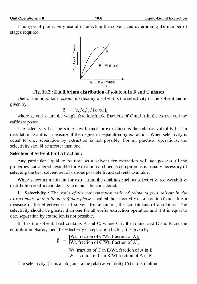
Unit Operations – II 10.6 Liquid-Liquid Extraction
This type of plot is very useful in selecting the solvent and determining the number of
stages required.
% C
in B
Phase
% C in A Phase
F - Plait point
F
Fig. 10.2 : Equilibrium distribution of solute A in B and C phases
One of the important factors in selecting a solvent is the selectivity of the solvent and is
given by
β = [xC/xA]E / [xC/xA]R
where xA and xB are the weight fractions/mole fractions of C and A in the extract and the
raffinate phase.
The selectivity has the same significance in extraction as the relative volatility has in
distillation. So it is a measure of the degree of separation by extraction. When selectivity is
equal to one, separation by extraction is not possible. For all practical operations, the
selectivity should be greater than one.
Selection of Solvent for Extraction :
Any particular liquid to be used as a solvent for extraction will not possess all the
properties considered desirable for extraction and hence compromise is usually necessary of
selecting the best solvent out of various possible liquid solvents available.
While selecting a solvent for extraction, the qualities such as selectivity, recoverability,
distribution coefficient, density, etc. must be considered.
1. Selectivity : The ratio of the concentration ratio of solute to feed solvent in the
extract phase to that in the raffinate phase is called the selectivity or separation factor. It is a
measure of the effectiveness of solvent for separating the constituents of a solution. The
selectivity should be greater than one for all useful extraction operation and if it is equal to
one, separation by extraction is not possible.
If B is the solvent, feed contains A and C, where C is the solute, and E and R are the
equilibrium phases, then the selectivity or separation factor, β is given by
β = [Wt. fraction of C/Wt. fraction of A]E
[Wt. fraction of C/Wt. fraction of A]R
= Wt. fraction of C in E/Wt. fraction of A in E
Wt. fraction of C in R/Wt.fraction of A in R
The selectivity (β) is analogous to the relative volatility (α) in distillation.

Unit Operations – II 10.7 Liquid-Liquid Extraction
2. Recoverability : As the solvent should be recovered for reuse frequently by
distillation, it should not form an azeotrope with the extracted solute for low cost recovery,
the relative volatility of the mixture formed should be high.
The latent heat of vaporisation of the solvent selected should be small whenever the
solvent is to be vaproised.
3. Distribution coefficient : Higher values (>1) of the distribution coefficient are
generally desirable as less solvent will then be required for a given extraction duty.
4. Density : The difference in densities of the saturated liquid phases should be larger
for ease is physical separation.
5. Insolubility of solvent : The solvent insoluble in the original liquid solvent should
be preferred. It should have a high solubility for the solute to be extracted as then small
amounts of the solvent are required.
6. Interfacial tension : Interfacial tension should be high for coalescence of emulsions
to occur more readily, as the same is of a greater importance than dispersion.
7. The solvent should be stable chemically. It should be inert towards the components
of the system.
8. It should not be corrosive towards common materials of construction.
9. The solvent should be cheap.
10. The solvent should be non-toxic and non-flammable.
11. The solvent should have a low viscosity, freezing point, vapour pressure for ease in
handling and storage.
Extraction Equipments :
In liquid-liquid extraction operation, the two phases must be brought into intimate
contact for mass transfer to occur and then the phases are separated. This operation may be
carried out batchwise or continuously. Whenever we are dealing with simple systems and
quantities to be handled are small, batchwise procedure is adopted and when large quantities
are to be handled and several contacts are required, continuous operation becomes
economical.
Most of the extraction equipments are operated continuously with either successive stage
contacts (stagewise contactors) or differential contacts (differential contactors).
Industrial extraction equipments are classified as :
1. Stage-type extractors and
2. Differential (continuous contact) extractors.
Mixer-settler (single and multistage), plate column, pulsed sieve plate column, etc. are
examples of stage-type extractor.
Packed column, spray column, pulsed packed column, rotating disc contactors, etc. are
examples of differential extractor.
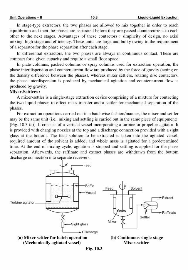
Unit Operations – II 10.8 Liquid-Liquid Extraction
In stage-type extractors, the two phases are allowed to mix together in order to reach
equilibrium and then the phases are separated before they are passed countercurrent to each
other to the next stages. Advantages of these contactors : simplicity of design, no axial
mixing, high stage and efficiency. These units are large and bulky owing to the requirement
of a separator for the phase separation after each stage.
In differential extractors, the two phases are always in continuous contact. These are
compact for a given capacity and require a small floor space.
In plate columns, packed columns or spray columns used for extraction operation, the
phase interdispersion and countercurrent flow are produced by the force of gravity (acting on
the density difference between the phases), whereas mixer settlers, rotating disc contactors,
the phase interdispersion is produced by mechanical agitation and countercurrent flow is
produced by gravity.
Mixer-Settlers :
A mixer-settler is a single-stage extraction device comprising of a mixture for contacting
the two liquid phases to effect mass transfer and a settler for mechanical separation of the
phases.
For extraction operations carried out in a batchwise fashion/manner, the mixer and settler
may be the same unit (i.e., mixing and settling is carried out in the same piece of equipment).
[Fig. 10.3 (a)]. It consists of a vertical vessel incorporating a turbine or propeller agitator. It
is provided with charging nozzles at the top and a discharge connection provided with a sight
glass at the bottom. The feed solution to be extracted is taken into the agitated vessel,
required amount of the solvent is added, and whole mass is agitated for a predetermined
time. At the end of mixing cycle, agitation is stopped and settling is applied for the phase
separation. Afterwards, the raffinate and extract phases are withdrawn from the bottom
discharge connection into separate receivers.
Feed
Sight glass
Discharge
Turbine agitator
Baffle
Vessel
Feed Solvent
Extract
Raffinate
Settler
Mixer
(a) Mixer settler for batch operation
(Mechanically agitated vessel)
(b) Continuous single-stage
Mixer-settler
Fig. 10.3
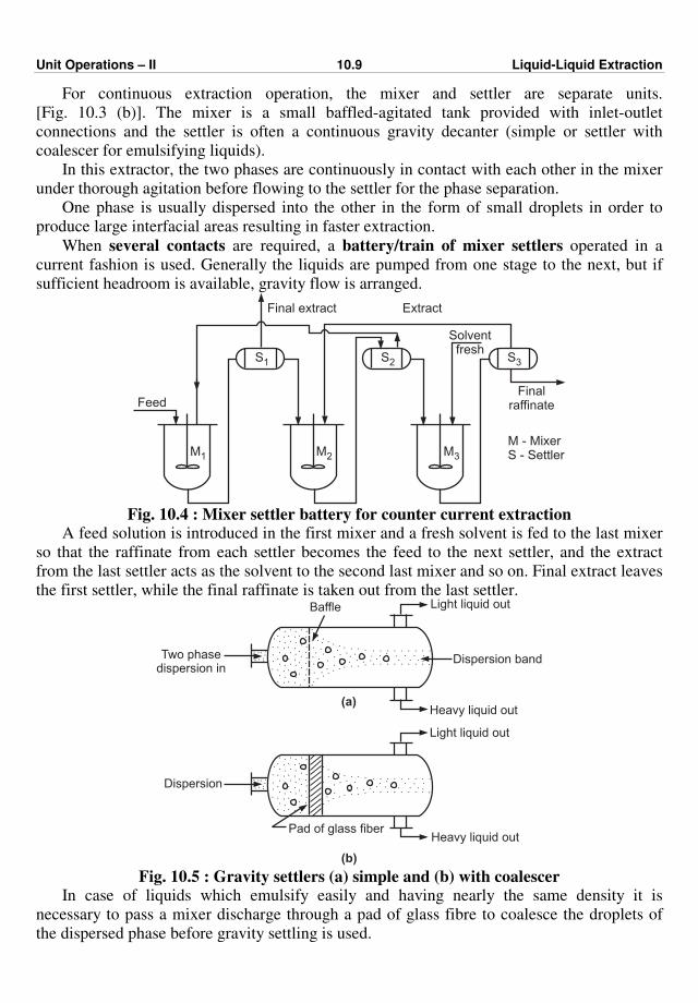
Unit Operations – II 10.9 Liquid-Liquid Extraction
For continuous extraction operation, the mixer and settler are separate units.
[Fig. 10.3 (b)]. The mixer is a small baffled-agitated tank provided with inlet-outlet
connections and the settler is often a continuous gravity decanter (simple or settler with
coalescer for emulsifying liquids).
In this extractor, the two phases are continuously in contact with each other in the mixer
under thorough agitation before flowing to the settler for the phase separation.
One phase is usually dispersed into the other in the form of small droplets in order to
produce large interfacial areas resulting in faster extraction.
When several contacts are required, a battery/train of mixer settlers operated in a
current fashion is used. Generally the liquids are pumped from one stage to the next, but if
sufficient headroom is available, gravity flow is arranged.
S1 S2
Final extract Extract
Solventfresh
S3
Finalraffinate
M - MixerS - SettlerM1 M2 M3
Feed
Fig. 10.4 : Mixer settler battery for counter current extraction
A feed solution is introduced in the first mixer and a fresh solvent is fed to the last mixer
so that the raffinate from each settler becomes the feed to the next settler, and the extract
from the last settler acts as the solvent to the second last mixer and so on. Final extract leaves
the first settler, while the final raffinate is taken out from the last settler. Baffle
Heavy liquid out
Dispersion band
(a)
Two phasedispersion in
Heavy liquid outPad of glass fiber
Dispersion
(b)
Light liquid out
Light liquid out
Fig. 10.5 : Gravity settlers (a) simple and (b) with coalescer In case of liquids which emulsify easily and having nearly the same density it is
necessary to pass a mixer discharge through a pad of glass fibre to coalesce the droplets of
the dispersed phase before gravity settling is used.
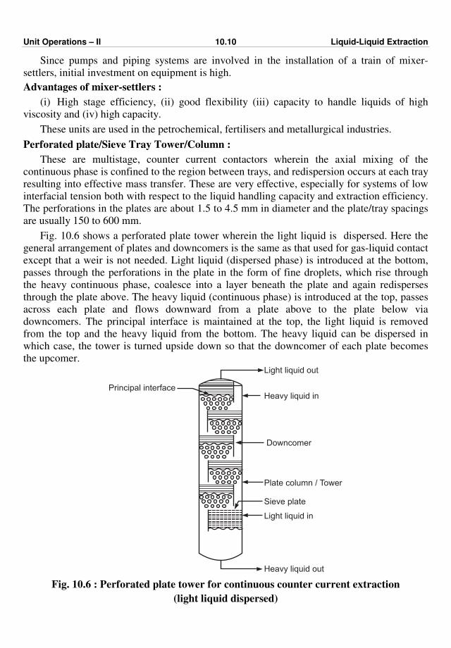
Unit Operations – II 10.10 Liquid-Liquid Extraction
Since pumps and piping systems are involved in the installation of a train of mixer-
settlers, initial investment on equipment is high.
Advantages of mixer-settlers :
(i) High stage efficiency, (ii) good flexibility (iii) capacity to handle liquids of high
viscosity and (iv) high capacity.
These units are used in the petrochemical, fertilisers and metallurgical industries.
Perforated plate/Sieve Tray Tower/Column :
These are multistage, counter current contactors wherein the axial mixing of the
continuous phase is confined to the region between trays, and redispersion occurs at each tray
resulting into effective mass transfer. These are very effective, especially for systems of low
interfacial tension both with respect to the liquid handling capacity and extraction efficiency.
The perforations in the plates are about 1.5 to 4.5 mm in diameter and the plate/tray spacings
are usually 150 to 600 mm.
Fig. 10.6 shows a perforated plate tower wherein the light liquid is dispersed. Here the
general arrangement of plates and downcomers is the same as that used for gas-liquid contact
except that a weir is not needed. Light liquid (dispersed phase) is introduced at the bottom,
passes through the perforations in the plate in the form of fine droplets, which rise through
the heavy continuous phase, coalesce into a layer beneath the plate and again redisperses
through the plate above. The heavy liquid (continuous phase) is introduced at the top, passes
across each plate and flows downward from a plate above to the plate below via
downcomers. The principal interface is maintained at the top, the light liquid is removed
from the top and the heavy liquid from the bottom. The heavy liquid can be dispersed in
which case, the tower is turned upside down so that the downcomer of each plate becomes
the upcomer.
Heavy liquid out
Light liquid in
Sieve plate
Plate column / Tower
Downcomer
Heavy liquid in
Light liquid out
Principal interface
Fig. 10.6 : Perforated plate tower for continuous counter current extraction
(light liquid dispersed)
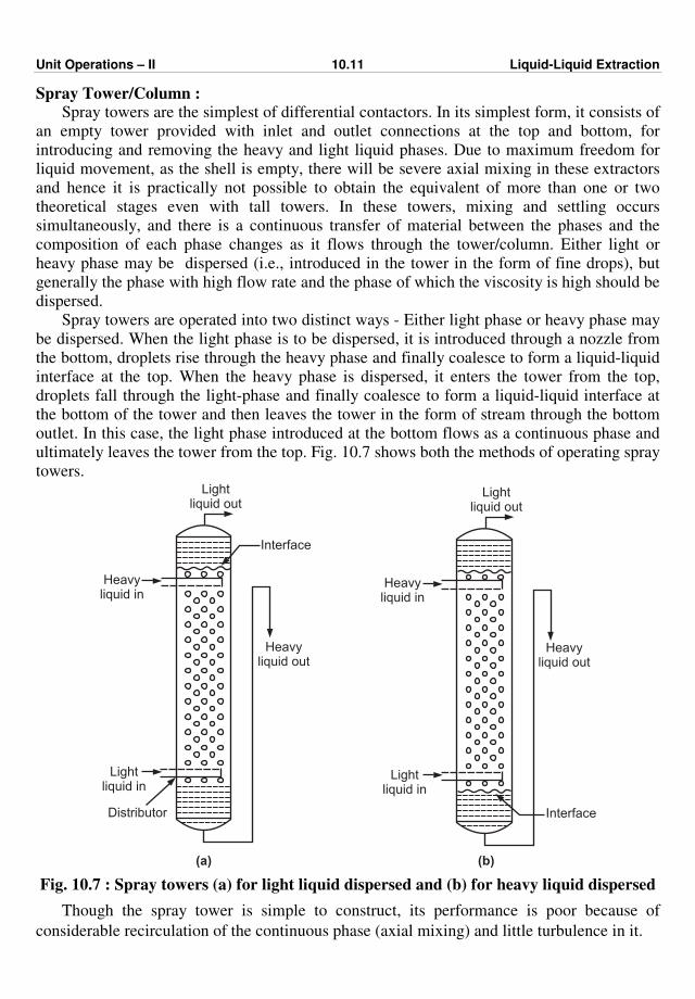
Unit Operations – II 10.11 Liquid-Liquid Extraction
Spray Tower/Column : Spray towers are the simplest of differential contactors. In its simplest form, it consists of
an empty tower provided with inlet and outlet connections at the top and bottom, for
introducing and removing the heavy and light liquid phases. Due to maximum freedom for
liquid movement, as the shell is empty, there will be severe axial mixing in these extractors
and hence it is practically not possible to obtain the equivalent of more than one or two
theoretical stages even with tall towers. In these towers, mixing and settling occurs
simultaneously, and there is a continuous transfer of material between the phases and the
composition of each phase changes as it flows through the tower/column. Either light or
heavy phase may be dispersed (i.e., introduced in the tower in the form of fine drops), but
generally the phase with high flow rate and the phase of which the viscosity is high should be
dispersed.
Spray towers are operated into two distinct ways - Either light phase or heavy phase may
be dispersed. When the light phase is to be dispersed, it is introduced through a nozzle from
the bottom, droplets rise through the heavy phase and finally coalesce to form a liquid-liquid
interface at the top. When the heavy phase is dispersed, it enters the tower from the top,
droplets fall through the light-phase and finally coalesce to form a liquid-liquid interface at
the bottom of the tower and then leaves the tower in the form of stream through the bottom
outlet. In this case, the light phase introduced at the bottom flows as a continuous phase and
ultimately leaves the tower from the top. Fig. 10.7 shows both the methods of operating spray
towers.
Distributor
Heavyliquid in
Lightliquid in
Heavyliquid out
Lightliquid out
Interface
Heavyliquid in
Lightliquid in
Heavyliquid out
Lightliquid out
Interface
(a) (b)
Fig. 10.7 : Spray towers (a) for light liquid dispersed and (b) for heavy liquid dispersed
Though the spray tower is simple to construct, its performance is poor because of
considerable recirculation of the continuous phase (axial mixing) and little turbulence in it.
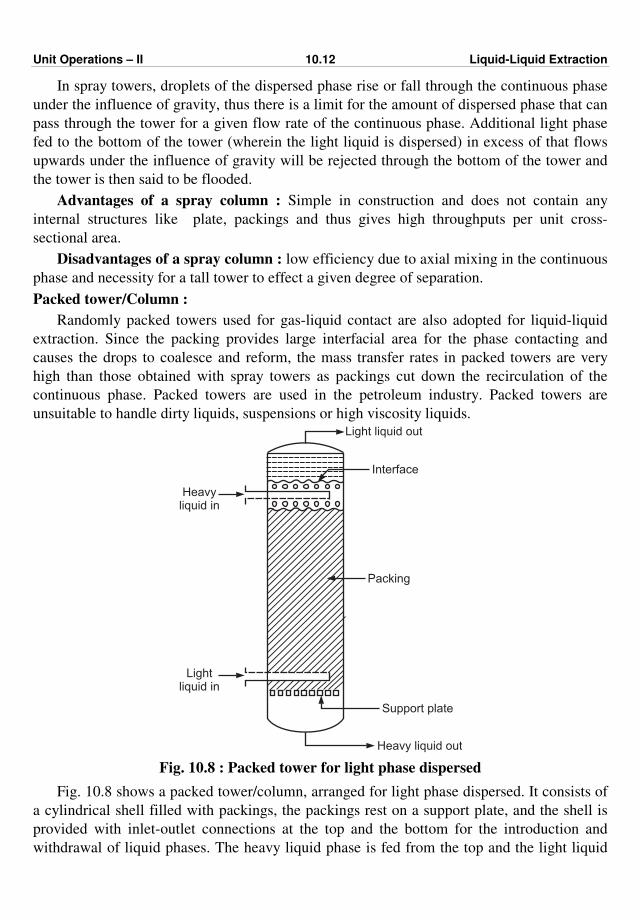
Unit Operations – II 10.12 Liquid-Liquid Extraction
In spray towers, droplets of the dispersed phase rise or fall through the continuous phase
under the influence of gravity, thus there is a limit for the amount of dispersed phase that can
pass through the tower for a given flow rate of the continuous phase. Additional light phase
fed to the bottom of the tower (wherein the light liquid is dispersed) in excess of that flows
upwards under the influence of gravity will be rejected through the bottom of the tower and
the tower is then said to be flooded.
Advantages of a spray column : Simple in construction and does not contain any
internal structures like plate, packings and thus gives high throughputs per unit cross-
sectional area.
Disadvantages of a spray column : low efficiency due to axial mixing in the continuous
phase and necessity for a tall tower to effect a given degree of separation.
Packed tower/Column :
Randomly packed towers used for gas-liquid contact are also adopted for liquid-liquid
extraction. Since the packing provides large interfacial area for the phase contacting and
causes the drops to coalesce and reform, the mass transfer rates in packed towers are very
high than those obtained with spray towers as packings cut down the recirculation of the
continuous phase. Packed towers are used in the petroleum industry. Packed towers are
unsuitable to handle dirty liquids, suspensions or high viscosity liquids.
Heavyliquid in
Lightliquid in
Support plate
Heavy liquid out
Interface
Light liquid out
Packing
Fig. 10.8 : Packed tower for light phase dispersed
Fig. 10.8 shows a packed tower/column, arranged for light phase dispersed. It consists of
a cylindrical shell filled with packings, the packings rest on a support plate, and the shell is
provided with inlet-outlet connections at the top and the bottom for the introduction and
withdrawal of liquid phases. The heavy liquid phase is fed from the top and the light liquid
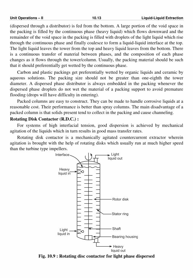
Unit Operations – II 10.13 Liquid-Liquid Extraction
(dispersed through a distributor) is fed from the bottom. A large portion of the void space in
the packing is filled by the continuous phase (heavy liquid) which flows downward and the
remainder of the void space in the packing is filled with droplets of the light liquid which rise
through the continuous phase and finally coalesce to form a liquid-liquid interface at the top.
The light liquid leaves the tower from the top and heavy liquid leaves from the bottom. There
is a continuous transfer of material between phases, and the composition of each phase
changes as it flows through the tower/column. Usually, the packing material should be such
that it should preferentially get wetted by the continuous phase.
Carbon and plastic packings get preferentially wetted by organic liquids and ceramic by
aqueous solutions. The packing size should not be greater than one-eighth the tower
diameter. A dispersed phase distributor is always embedded in the packing whenever the
dispersed phase droplets do not wet the material of a packing support to avoid premature
flooding (drops will have difficulty in entering).
Packed columns are easy to construct. They can be made to handle corrosive liquids at a
reasonable cost. Their performance is better than spray columns. The main disadvantage of a
packed column is that solids present tend to collect in the packing and cause channeling.
Rotating Disk Contactor (R.D.C.) :
For systems of high interfacial tension, good dispersion is achieved by mechanical
agitation of the liquids which in turn results in good mass transfer rates.
Rotating disk contactor is a mechanically agitated countercurrent extractor wherein
agitation is brought with the help of rotating disks which usually run at much higher speed
than the turbine type impellers.
Heavyliquid in
Lightliquid out
Heavyliquid out
Interface
Lightliquid in
Bearing housing
Shaft
Stator ring
Rotor disk
Fig. 10.9 : Rotating disc contactor for light phase dispersed
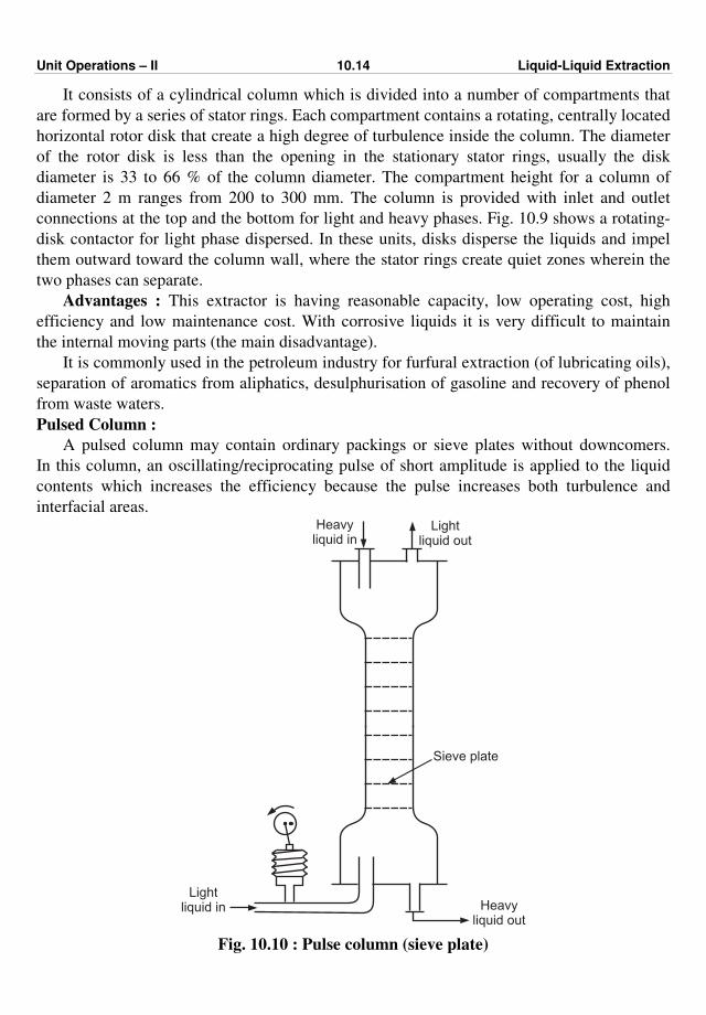
Unit Operations – II 10.14 Liquid-Liquid Extraction
It consists of a cylindrical column which is divided into a number of compartments that
are formed by a series of stator rings. Each compartment contains a rotating, centrally located
horizontal rotor disk that create a high degree of turbulence inside the column. The diameter
of the rotor disk is less than the opening in the stationary stator rings, usually the disk
diameter is 33 to 66 % of the column diameter. The compartment height for a column of
diameter 2 m ranges from 200 to 300 mm. The column is provided with inlet and outlet
connections at the top and the bottom for light and heavy phases. Fig. 10.9 shows a rotating-
disk contactor for light phase dispersed. In these units, disks disperse the liquids and impel
them outward toward the column wall, where the stator rings create quiet zones wherein the
two phases can separate.
Advantages : This extractor is having reasonable capacity, low operating cost, high
efficiency and low maintenance cost. With corrosive liquids it is very difficult to maintain
the internal moving parts (the main disadvantage).
It is commonly used in the petroleum industry for furfural extraction (of lubricating oils),
separation of aromatics from aliphatics, desulphurisation of gasoline and recovery of phenol
from waste waters.
Pulsed Column :
A pulsed column may contain ordinary packings or sieve plates without downcomers.
In this column, an oscillating/reciprocating pulse of short amplitude is applied to the liquid
contents which increases the efficiency because the pulse increases both turbulence and
interfacial areas.
Heavyliquid out
Lightliquid out
Heavyliquid in
Lightliquid in
Sieve plate
Fig. 10.10 : Pulse column (sieve plate)
Unit Operations – II 10.15 Liquid-Liquid Extraction
A reciprocating pump is a common mechanically pulsing device which pulses the entire
contents of the column at a frequent intervals, owing to which a rapid reciprocating motion
of relatively small amplitude is superimposed on usual flow of the liquid phases. Bellows or
diaphrams of steel, teflon, etc. are also used as pulsing devices.
A pulsed sieve plate column consists of a vertical column with a large number of sieve
plates without downcomers. The perforations in the plates of such columns are smaller than
nonpulsing columns (1.5 to 3 mm diameter). Pulsing amplitudes of 5 to 25 mm are generally
recommended with frequencies of 100 to 260 cycles/minute. The pulsation causes the light
liquid to be dispersed into the heavy phase on the upward stroke and the heavy liquid phase
to jet into the light phase on the downward stroke. The column has no moving parts, low
axial mixing and high extraction efficiency.
A pulsed packed column consists of a vertical column filled with packings.
In pulse columns (either sieve plate or packed) the height required for a given number of
theoretical contacts is often less than one-third that needed in a nonpulsing column.
Pulse columns are extensively used for processing radioactive solutions in atomic-energy
work. They are also used in petrochemical and metallurgical industries.
SOLVED EXAMPLES
Example 10.1 : Picric acid is to be extracted with benzene from its solution. If the
aqueous solution contains 0.2 mol of picric acid 1 per litre, calculate the volume of benzene
with which 1 litre of the solution must be extracted in order to form a benzene solution
containing 0.02 mol of picric acid per litre (Neglect the difference between the volume of the
solution and that of pure solvent). Also calculate the percent recovery of picric acid from the
aqueous solution.
K = distribution coefficient = CE/CR = 0.505
where CE = concentration of picric acid in benzene, mol per litre of solution
CR = concentration of picric acid in water, mol per litre of solution
Solution : Basis : 1 litre original aqueous solution. It contains 0.2 mol of picric acid.
Given : K = 0.505 = CE/CR
Final concentration of picric acid
in the aqueous solution = CR = CE/K = 0.02
0.505
= 0.0396 mol/l
Picric acid in the final benzene solution = 0.20 – 0.0396
= 0.16 mol
Benzene required = 0.16
0.02
= 8 l per l of aqueous solution … Ans.
% extraction of picric acid = 0.16
0.20 × 100
= 80 % … Ans.
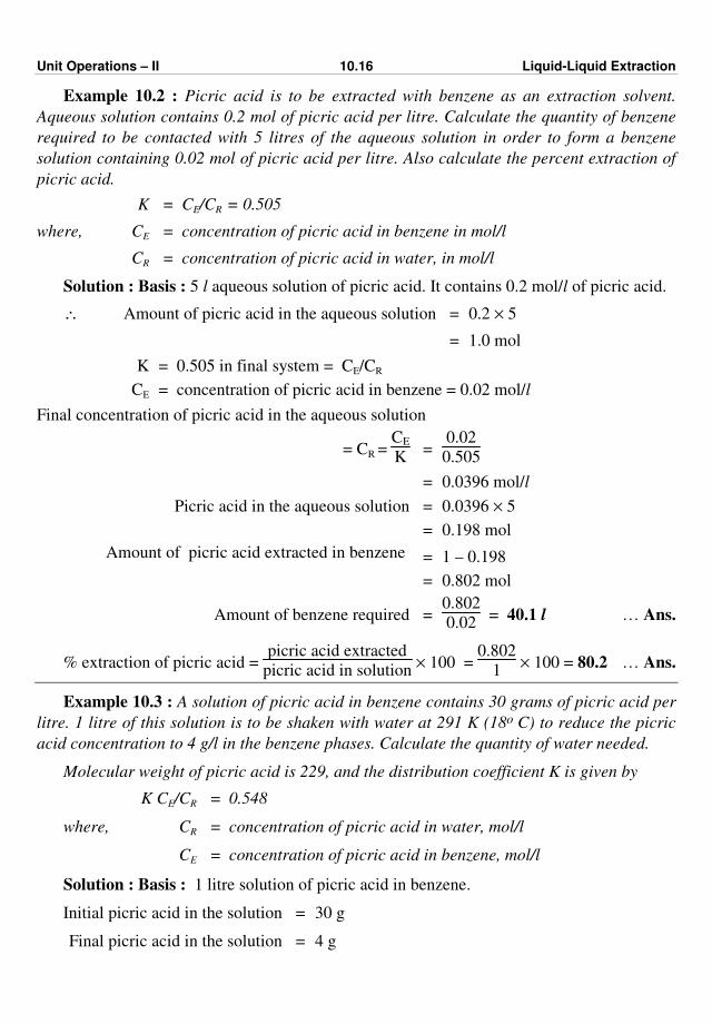
Unit Operations – II 10.16 Liquid-Liquid Extraction
Example 10.2 : Picric acid is to be extracted with benzene as an extraction solvent.
Aqueous solution contains 0.2 mol of picric acid per litre. Calculate the quantity of benzene
required to be contacted with 5 litres of the aqueous solution in order to form a benzene
solution containing 0.02 mol of picric acid per litre. Also calculate the percent extraction of
picric acid.
K = CE/CR = 0.505
where, CE = concentration of picric acid in benzene in mol/l
CR = concentration of picric acid in water, in mol/l
Solution : Basis : 5 l aqueous solution of picric acid. It contains 0.2 mol/l of picric acid.
∴ Amount of picric acid in the aqueous solution = 0.2 × 5
= 1.0 mol
K = 0.505 in final system = CE/CR
CE = concentration of picric acid in benzene = 0.02 mol/l
Final concentration of picric acid in the aqueous solution
= CR = CE
K =
0.02
0.505
= 0.0396 mol/l
Picric acid in the aqueous solution = 0.0396 × 5
= 0.198 mol
Amount of picric acid extracted in benzene = 1 – 0.198
= 0.802 mol
Amount of benzene required = 0.802
0.02 = 40.1 l … Ans.
% extraction of picric acid = picric acid extracted
picric acid in solution × 100 =
0.802
1 × 100 = 80.2 … Ans.
Example 10.3 : A solution of picric acid in benzene contains 30 grams of picric acid per
litre. 1 litre of this solution is to be shaken with water at 291 K (18o C) to reduce the picric
acid concentration to 4 g/l in the benzene phases. Calculate the quantity of water needed.
Molecular weight of picric acid is 229, and the distribution coefficient K is given by
K CE/CR = 0.548
where, CR = concentration of picric acid in water, mol/l
CE = concentration of picric acid in benzene, mol/l
Solution : Basis : 1 litre solution of picric acid in benzene.
Initial picric acid in the solution = 30 g
Final picric acid in the solution = 4 g
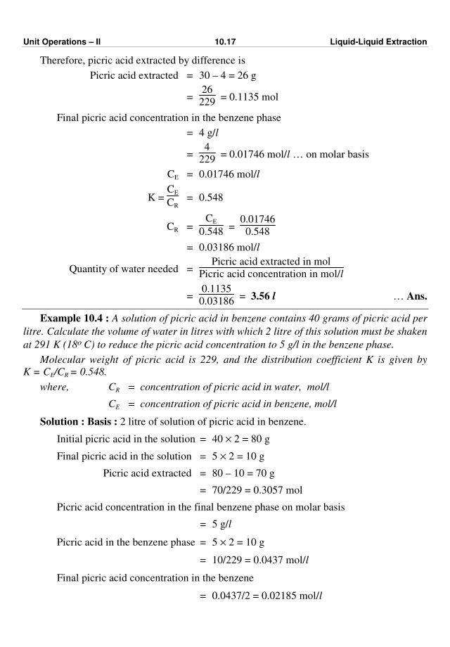
Unit Operations – II 10.17 Liquid-Liquid Extraction
Therefore, picric acid extracted by difference is
Picric acid extracted = 30 – 4 = 26 g
= 26
229 = 0.1135 mol
Final picric acid concentration in the benzene phase
= 4 g/l
= 4
229 = 0.01746 mol/l … on molar basis
CE = 0.01746 mol/l
K = CE
CR = 0.548
CR = CE
0.548 =
0.01746
0.548
= 0.03186 mol/l
Quantity of water needed = Picric acid extracted in mol
Picric acid concentration in mol/l
= 0.1135
0.03186 = 3.56 l … Ans.
Example 10.4 : A solution of picric acid in benzene contains 40 grams of picric acid per
litre. Calculate the volume of water in litres with which 2 litre of this solution must be shaken
at 291 K (18o C) to reduce the picric acid concentration to 5 g/l in the benzene phase.
Molecular weight of picric acid is 229, and the distribution coefficient K is given by
K = CE/CR = 0.548.
where, CR = concentration of picric acid in water, mol/l
CE = concentration of picric acid in benzene, mol/l
Solution : Basis : 2 litre of solution of picric acid in benzene.
Initial picric acid in the solution = 40 × 2 = 80 g
Final picric acid in the solution = 5 × 2 = 10 g
Picric acid extracted = 80 – 10 = 70 g
= 70/229 = 0.3057 mol
Picric acid concentration in the final benzene phase on molar basis
= 5 g/l
Picric acid in the benzene phase = 5 × 2 = 10 g
= 10/229 = 0.0437 mol/l
Final picric acid concentration in the benzene
= 0.0437/2 = 0.02185 mol/l
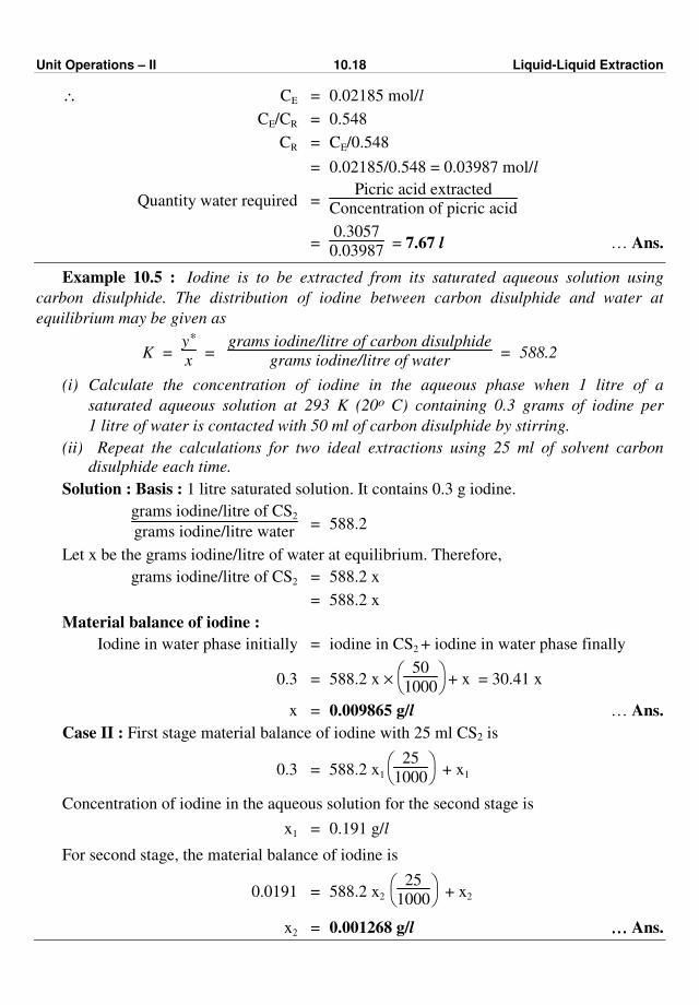
Unit Operations – II 10.18 Liquid-Liquid Extraction
∴ CE = 0.02185 mol/l
CE/CR = 0.548
CR = CE/0.548
= 0.02185/0.548 = 0.03987 mol/l
Quantity water required = Picric acid extracted
Concentration of picric acid
= 0.3057
0.03987 = 7.67 l … Ans.
Example 10.5 : Iodine is to be extracted from its saturated aqueous solution using
carbon disulphide. The distribution of iodine between carbon disulphide and water at
equilibrium may be given as
K = y*
x =
grams iodine/litre of carbon disulphide
grams iodine/litre of water = 588.2
(i) Calculate the concentration of iodine in the aqueous phase when 1 litre of a
saturated aqueous solution at 293 K (20o C) containing 0.3 grams of iodine per
1 litre of water is contacted with 50 ml of carbon disulphide by stirring.
(ii) Repeat the calculations for two ideal extractions using 25 ml of solvent carbon
disulphide each time.
Solution : Basis : 1 litre saturated solution. It contains 0.3 g iodine.
grams iodine/litre of CS2
grams iodine/litre water = 588.2
Let x be the grams iodine/litre of water at equilibrium. Therefore,
grams iodine/litre of CS2 = 588.2 x
= 588.2 x
Material balance of iodine :
Iodine in water phase initially = iodine in CS2 + iodine in water phase finally
0.3 = 588.2 x ×
50
1000 + x = 30.41 x
x = 0.009865 g/l … Ans.
Case II : First stage material balance of iodine with 25 ml CS2 is
0.3 = 588.2 x1
25
1000 + x1
Concentration of iodine in the aqueous solution for the second stage is
x1 = 0.191 g/l
For second stage, the material balance of iodine is
0.0191 = 588.2 x2
25
1000 + x2
x2 = 0.001268 g/l ………… Ans.
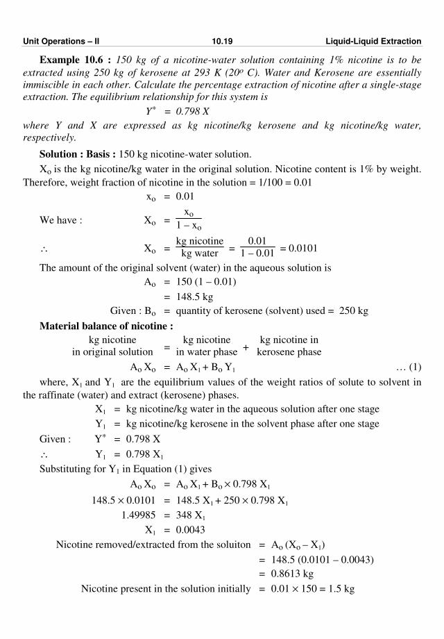
Unit Operations – II 10.19 Liquid-Liquid Extraction
Example 10.6 : 150 kg of a nicotine-water solution containing 1% nicotine is to be
extracted using 250 kg of kerosene at 293 K (20o C). Water and Kerosene are essentially
immiscible in each other. Calculate the percentage extraction of nicotine after a single-stage
extraction. The equilibrium relationship for this system is
Y* = 0.798 X
where Y and X are expressed as kg nicotine/kg kerosene and kg nicotine/kg water,
respectively.
Solution : Basis : 150 kg nicotine-water solution.
Xo is the kg nicotine/kg water in the original solution. Nicotine content is 1% by weight.
Therefore, weight fraction of nicotine in the solution = 1/100 = 0.01
xo = 0.01
We have : Xo = xo
1 – xo
∴ Xo = kg nicotine
kg water =
0.01
1 – 0.01 = 0.0101
The amount of the original solvent (water) in the aqueous solution is
Ao = 150 (1 – 0.01)
= 148.5 kg
Given : Bo = quantity of kerosene (solvent) used = 250 kg
Material balance of nicotine :
kg nicotine
in original solution = kg nicotine
in water phase + kg nicotine in
kerosene phase
Ao Xo = Ao X1 + Bo Y1 … (1)
where, X1 and Y1 are the equilibrium values of the weight ratios of solute to solvent in
the raffinate (water) and extract (kerosene) phases.
X1 = kg nicotine/kg water in the aqueous solution after one stage
Y1 = kg nicotine/kg kerosene in the solvent phase after one stage
Given : Y* = 0.798 X
∴ Y1 = 0.798 X1
Substituting for Y1 in Equation (1) gives
Ao Xo = Ao X1 + Bo × 0.798 X1
148.5 × 0.0101 = 148.5 X1 + 250 × 0.798 X1
1.49985 = 348 X1
X1 = 0.0043
Nicotine removed/extracted from the soluiton = Ao (Xo – X1)
= 148.5 (0.0101 – 0.0043)
= 0.8613 kg
Nicotine present in the solution initially = 0.01 × 150 = 1.5 kg

Unit Operations – II 10.20 Liquid-Liquid Extraction
% extraction of nicotine = Nicotine extracted
Nicotine in the original solution × 100
= 0.8613
1.5 × 100
= 57.42 … Ans.
Example 10.7 : The picric acid is to be extracted with benzene. If the aqueous solution
contains 0.20 mol of picric acid per litre, calculate the volume of benzene with which 1 litre
of this solution must be extracted to form a benzene solution containing 0.01 mol of picric
acid per litre. Also calculate the percentage recovery of picric acid from the aqueous
solution.
K = distribution coefficient at 288 K (15 oC)
K = CE/CR = 0.705
where, CR = concentration of picric acid in water in mol/l
CE = concentration of picric acid in benzene in mol/l
Solution : Basis : 1 litre original aqueous solution. It contains 0.2 mol of picric acid.
K = 0.705 in final system = CE/CR
CE = concentration of picric acid in benzene = 0.01 mol/l
Benzene required = Picric acid in benzene phase in mol
Concentration of picric acid in benzene phase in mol/l
Final concentration of picric
acid in the aqueous solution = 0.01
0.705
= 0.01418 mol/l
[CR = CE/K]
Picric acid in the final benzene solution = 0.20 – 0.01418
= 0.18582 mol
∴ Benzene required = 0.18582
0.01
= 18.582 l ………… Ans.
% extraction of picric acid = picric acid extracted
picric acid in the original solution × 100
= 0.18582
0.2 × 100 = 92.91 ………… Ans.
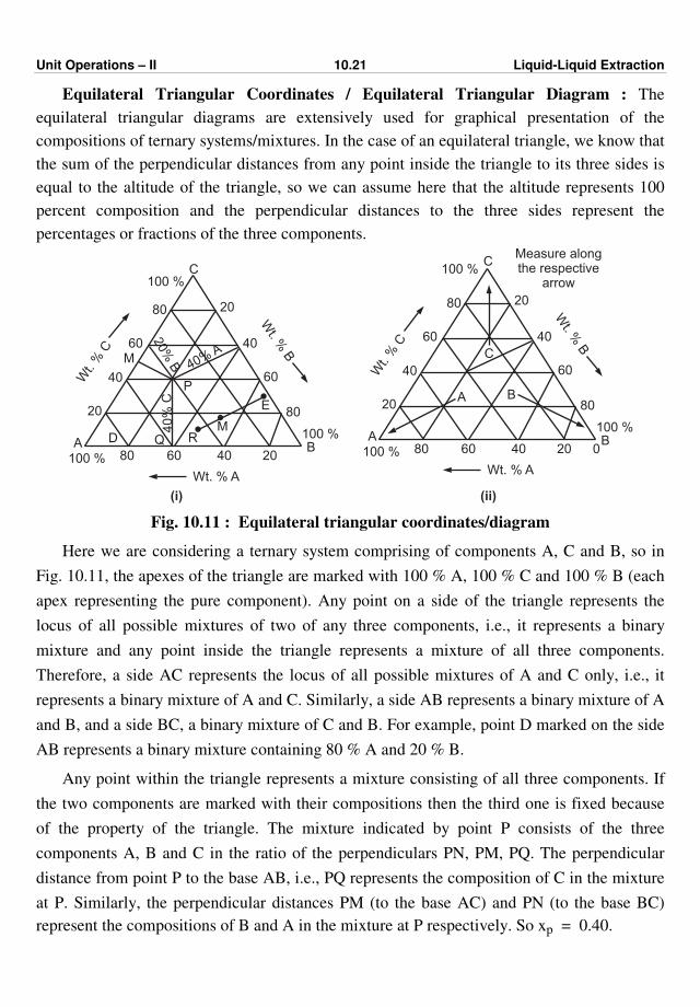
Unit Operations – II 10.21 Liquid-Liquid Extraction
Equilateral Triangular Coordinates / Equilateral Triangular Diagram : The
equilateral triangular diagrams are extensively used for graphical presentation of the
compositions of ternary systems/mixtures. In the case of an equilateral triangle, we know that
the sum of the perpendicular distances from any point inside the triangle to its three sides is
equal to the altitude of the triangle, so we can assume here that the altitude represents 100
percent composition and the perpendicular distances to the three sides represent the
percentages or fractions of the three components.
Wt.
%C
100 %C
A B100 %
100 % 80 60 40 20
Wt. % A
20
40
60
80
Wt. %
B
20
40
60
80
BA
C
0
Measure alongthe respective
arrow
(ii)
Wt.
%C
100 %C
A B100 %
100 % 80 60 40 20
Wt. % A
E
RQ
20
40
60
80
Wt. %
B
40%A
20%
B
P
40%
C
D
20
40
60
80
M
(i)
M
Fig. 10.11 : Equilateral triangular coordinates/diagram
Here we are considering a ternary system comprising of components A, C and B, so in
Fig. 10.11, the apexes of the triangle are marked with 100 % A, 100 % C and 100 % B (each
apex representing the pure component). Any point on a side of the triangle represents the
locus of all possible mixtures of two of any three components, i.e., it represents a binary
mixture and any point inside the triangle represents a mixture of all three components.
Therefore, a side AC represents the locus of all possible mixtures of A and C only, i.e., it
represents a binary mixture of A and C. Similarly, a side AB represents a binary mixture of A
and B, and a side BC, a binary mixture of C and B. For example, point D marked on the side
AB represents a binary mixture containing 80 % A and 20 % B.
Any point within the triangle represents a mixture consisting of all three components. If
the two components are marked with their compositions then the third one is fixed because
of the property of the triangle. The mixture indicated by point P consists of the three
components A, B and C in the ratio of the perpendiculars PN, PM, PQ. The perpendicular
distance from point P to the base AB, i.e., PQ represents the composition of C in the mixture
at P. Similarly, the perpendicular distances PM (to the base AC) and PN (to the base BC)
represent the compositions of B and A in the mixture at P respectively. So xp = 0.40.
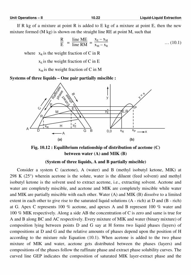
Unit Operations – II 10.22 Liquid-Liquid Extraction
If R kg of a mixture at point R is added to E kg of a mixture at point E, then the new
mixture formed (M kg) is shown on the straight line RE at point M, such that
R
E =
line ME
line RM =
xE – xM
xM – xR … (10.1)
where xR is the weight fraction of C in R
xE is the weight fraction of C in E
xM is the weight fraction of C in M
Systems of three liquids – One pair partially miscible :
P
y = x
xPxR x
E,R
0,0
y
yE*
yE*xR H
DAG B
A
M
R
C
P
Raffi
nate
phase B
Ext
ract
phas
e
E
(a) (b)
Fig. 10.12 : Equilibrium relationship of distribution of acetone (C)
between water (A) and MIK (B)
(System of three liquids, A and B partially miscible)
Consider a system C (acetone), A (water) and B (methyl isobutyl ketone, MIK) at
298 K (25°) wherein acetone is the solute, water is the diluent (feed solvent) and methyl
isobutyl ketone is the solvent used to extract acetone, i.e., extracting solvent. Acetone and
water are completely miscible, and acetone and MIK are completely miscible while water
and MIK are partially miscible with each other. Water (A) and MIK (B) dissolve to a limited
extent in each other to give rise to the saturated liquid solutions (A - rich) at D and (B - rich)
at G. Apex C represents 100 % acetone, and apexes A and B represent 100 % water and
100 % MIK respectively. Along a side AB the concentration of C is zero and same is true for
A and B along BC and AC respectively. Every mixture of MIK and water (binary mixture) of
composition lying between points D and G say at H forms two liquid phases (layers) of
compositions at D and G and the relative amounts of phases depend upon the position of H
according to the mixture rule Equation (10.1). When acetone is added to the two phase
mixture of MIK and water, acetone gets distributed between the phases (layers) and
compositions of the phases follow the raffinate phase and extract phase solubility curves. The
curved line GEP indicates the composition of saturated MIK layer-extract phase and the

Unit Operations – II 10.23 Liquid-Liquid Extraction
curved line DRP indicates the composition of saturated water layer-raffinate phase. The area
under the binodal solubility curve represented by curved line DRPEG represents a two phase
region that will split into two phases/layers in equilibrium with each other. Any mixture
outside this curve will be a homogeneous solution of one liquid phase. The equilibrium
compositions of two phases will lie on this curve. Any mixture underneath the curve at point
M will split into two saturated liquid phases of equilibrium compositions indicated by points
R and E. The line joining the equilibrium compositions of two phases (raffinate and extract)
i.e. line RE is called as a tie line. The tie line is one which connects together two phases in
equilibrium with each other. The points of a tie line must be found by experiment. The point
P on the binodal solubility curve represents a single phase which does not split into two
phases (i.e., at this point, phases become identical) and at this point A-rich and B-rich curves
merge; so the point P corresponds to a tie line of zero length and is known as a plait point. At
a given temperature and pressure point P is fixed. It is not necessary that the plait point be at
the peak of the binodal solubility curve and tie lines be parallel. In the system under
consideration wherein C is the solute and B is the extraction solvent, the separation will
increase as the plait point approaches A and tie lines increase in slope.
From Fig. 10.12, it is clear that % of C in E (extract) is greater than in R (raffinate) and
so in this case the distribution of C favours the B-rich phase (extract phase). This is shown on
the distribution diagram wherein the composition of C in the extract phase is plotted against
the composition of C in the raffinate phase (composition expressed in terms of weight
fraction). In Fig. 10.12 (b), the point E, R lies above the diagonal y = x indicating that y* is
always greater than x.
Thus, the distribution coefficient y*/x is greater than unity. When the concentration of C
at the ends of tie lines are plotted on the x - y diagram, we get the distribution curve as
shown in Fig. 10.12 (b).
For the ternary systems of the type described above, the mutual solubility of A and B
increases with increase in temperature and at one particular critical solution temperature they
get dissolved completely. So liquid extraction operations that depend upon formation of
insoluble liquid phases must be carried below such temperatures.
EXERCISES
1. Define liquid extraction and state briefly the fields of application of extraction.
2. Define the following terms with reference to extraction
(i) feed, (ii) solvent (iii) raffinate and (iv) extract.
3. Explain in briefly the selection criteria for solvent to be used for liquid-liquid
extraction.
4. Define selectivity and state what it indicates ?
Unit Operations – II 10.24 Liquid-Liquid Extraction
5. Explain in brief, triangular diagram for a ternary system with one pair partially
miscible.
6. Give the construction and working of a batch operated mixer-settler with a neat
sketch.
7. Explain briefly the mixer-settler assembly operated in a counter current fashion
with a sketch. State advantages of mixer-settlers.
8. Explain in brief the construction and operation of a sieve plate column for
extraction.
9. Write briefly on classification of extraction equipments.
10. Discuss in brief with a neat sketch the following equipments used for liquid-liquid
extraction.
(a) packed column, (b) spray column, (c) pulsed column.
11. Explain the construction of rotating-disk contactor with its neat sketch.
12. Differentiate between distillation and extraction.
ppp

(11.1)
CHAPTER ELEVEN
CRYSTALLISATION
In this chapter, our discussion is restricted to crystallisation from solution.
Crystallisation is an operation in which solid particles are formed from a liquid solution.
It is a solid-liquid operation used to separate a solute from its solution in the form of
crystals. In this operation, mass is transferred from the liquid phase (solution) to a pure solid
crystalline phase.
Crystallisation is an important operation in the chemical industry as the number of
salable products have to be in the form of crystals. This operation gives almost pure product
in the form of crystals of a desired size ranging from relatively impure solutions in a single
processing step. From the energy point of view, crystallisation requires much less energy for
separation as compared to other purification methods (e.g., distillation). It may be carried out
at relatively low temperatures and on a scale ranging from a few grams to thousands of tons
per day.
Crystallisation usually involves : (i) concentration of solution (by evaporating a part of
the solvent) and (ii) cooling of solution until the concentration of solute becomes higher than
its solubility at the prevailing temperature. The solute then comes out of the solution
(i.e., precipitates) in the form of pure crystals.
The performance of crystallisation process is evaluated in terms of size, shape, structure,
yield and purity of crystals. So in commercial crystallisation, the size and shape of crystals
are as important as the yield and purity of crystals.
Solubility :
The solubility of a solute in a given solvent is the concentration of the solute in a
saturated solution at a given temperature.
The concentration of a solute in a saturated solution is called the solubility of the solute
in the solvent.
The solubility of a solute in a given solvent depends on the nature of the solute, the
nature of the solvent and the prevailing temperature (solubility mainly depends on
temperature). Solubility data are generally given as parts by weight of anhydrous solute
material per 100 parts by weight of the solvent, e.g., the solubility of MgSO4 in water at
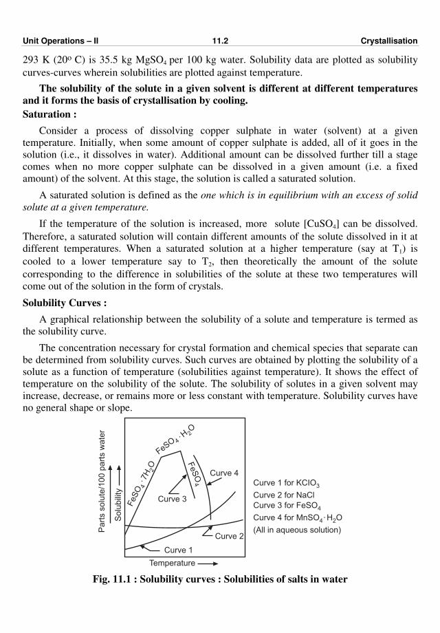
Unit Operations – II 11.2 Crystallisation
293 K (20o C) is 35.5 kg MgSO4 per 100 kg water. Solubility data are plotted as solubility
curves-curves wherein solubilities are plotted against temperature.
The solubility of the solute in a given solvent is different at different temperatures
and it forms the basis of crystallisation by cooling.
Saturation :
Consider a process of dissolving copper sulphate in water (solvent) at a given
temperature. Initially, when some amount of copper sulphate is added, all of it goes in the
solution (i.e., it dissolves in water). Additional amount can be dissolved further till a stage
comes when no more copper sulphate can be dissolved in a given amount (i.e. a fixed
amount) of the solvent. At this stage, the solution is called a saturated solution.
A saturated solution is defined as the one which is in equilibrium with an excess of solid
solute at a given temperature.
If the temperature of the solution is increased, more solute [CuSO4] can be dissolved.
Therefore, a saturated solution will contain different amounts of the solute dissolved in it at
different temperatures. When a saturated solution at a higher temperature (say at T1) is
cooled to a lower temperature say to T2, then theoretically the amount of the solute
corresponding to the difference in solubilities of the solute at these two temperatures will
come out of the solution in the form of crystals.
Solubility Curves :
A graphical relationship between the solubility of a solute and temperature is termed as
the solubility curve.
The concentration necessary for crystal formation and chemical species that separate can
be determined from solubility curves. Such curves are obtained by plotting the solubility of a
solute as a function of temperature (solubilities against temperature). It shows the effect of
temperature on the solubility of the solute. The solubility of solutes in a given solvent may
increase, decrease, or remains more or less constant with temperature. Solubility curves have
no general shape or slope.
Part
s s
olu
te/1
00 p
art
s w
ate
r
Solu
bili
ty
Temperature
Curve 1
Curve 2
Curve 3
Curve 4
FeS
O4
FeSO 4. H
O2
. 7H
O2
FeS
O4
Curve 1 for KCIO
Curve 2 for NaCl
3
Curve 3 for FeSO
Curve 4 for MnSO . H O
(All in aqueous solution)
4
4 2
Fig. 11.1 : Solubility curves : Solubilities of salts in water
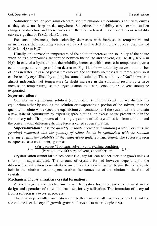
Unit Operations – II 11.3 Crystallisation
Solubility curves of potassium chlorate, sodium chloride are continuous solubility curves
as they show no sharp breaks anywhere. Sometime, the solubility curve exhibit sudden
changes of direction and these curves are therefore referred to as discontinuous solubility
curves, e.g., that of FeSO4, Na2SO4, etc.
For some substances, their solubility decreases with increase in temperature and
in such cases their solubility curves are called as inverted solubility curves (e.g., that of
MnSO4 · H2O in H2O).
Usually, an increase in temperature of the solution increases the solubility of the solute
when no true compounds are formed between the solute and solvent, e.g., KClO3, KNO3 in
H2O. In case of a hydrated salt, the solubility increases with increase in temperature over a
certain temperature range and then decreases. Fig. 11.1 shows solubility curves for a number
of salts in water. In case of potassium chlorate, the solubility increases with temperature so it
can be readily crystallised by cooling its saturated solution. The solubility of NaCl in water is
almost independent of temperature (a slight increase in the solubility results by a large
increase in temperature), so for crystallisation to occur, some of the solvent should be
evaporated.
Supersaturation :
Consider an equilibrium solution (solid solute + liquid solvent). If we disturb this
equilibrium either by cooling the solution or evaporating a portion of the solvent, then the
quantity of solute will exceed the equilibrium concentration and the system will try to attain
a new state of equilibrium by expelling (precipitating) an excess solute present in it in the
form of crystals. This process of forming crystals is called crystallisation from solution and
the concentration difference driving force is called supersaturation.
Supersaturation : It is the quantity of solute present in a solution (in which crystals are
growing) compared with the quantity of solute that is in equilibrium with the solution
(i.e., the equilibrium solubility at the temperature under consideration). The supersaturation
is expressed as a coefficient, given as
s = (Parts solute / 100 parts solvent) at prevailing condition
(Parts solute / 100 parts solvent) at equilibrium ≥ 1.0
Crystallisation cannot take place/occur (i.e., crystals can neither form nor grow) unless a
solution is supersaturated. The amount of crystals formed however depend upon the
difference in saturation concentration since once the crystallisation begins the extra solute
held in the solution due to supersaturation also comes out of the solution in the form of
crystals.
Mechanism of crystallisation / crystal formation :
A knowledge of the mechanism by which crystals form and grow is required in the
design and operation of an equipment used for crystallisation. The formation of a crystal
from a solution is a two-step process.
The first step is called nucleation (the birth of new small particles or nuclei) and the
second one is called crystal growth (growth of crystals to macroscopic size).
Unit Operations – II 11.4 Crystallisation
The generation of a new solid phase (i.e., new small particles) either on an inert material
in the solution or in the solution itself is called nucleation. The increase in size of these
nuclei with a layer-by-layer addition of solute is called crystal growth. Supersaturation is the
common driving force for nucleation and crystal growth. Crystals can neither form nor grow
unless a solution is supersaturated.
The number of nuclei formed and the rate of growth of crystals depend upon the
temperature of operation. The number of nuclei and growth rate of crystals increase with
increase in temperature upto a certain point and then decreases. The temperature
corresponding to a maximum number of nuclei formation is different than the temperature at
which a growth rate is maximum.
If initially a large number of nuclei is formed, then the yield of the process contains many
small or tiny crystals and if a few nuclei are formed initially (at the start), then the yield of
the process contains large size crystals. Slow cooling results in the formation of a less
number of nuclei and hence large size crystals are formed (as the material deposits on a
relatively few nuclei), whereas rapid cooling results in the/leads to the formation of a large
number of nuclei, giving the yield containing a large number of tiny crystals.
Methods of Supersaturation :
Unless a solution is supersaturated, neither nucleation nor crystal growth occurs
(i.e., crystals can neither form nor grow). Thus, for crystallisation to occur, supersaturation
can be generated by any one of the following methods :
(a) By cooling a concentrated, hot solution through indirect heat exchange.
(b) By evaporating a part of the solvent/By evaporating a solution.
(c) By adiabatic evaporation and cooling (i.e., by vacuum cooling) : by flashing of a
feed solution adiabatically to a lower temperature and inducing/causing
crystallisation by simultaneous cooling and evaporation of the solvent.
(d) By adding a new substance (i.e., a third substance) which reduces the solubility of
the original solute, i.e., by salting.
(e) By chemical reaction with a third substance.
When the solubility of the solute increases with increase in temperature, a saturated
solution becomes supersaturated, i.e., supersaturation is generated by cooling and
temperature reduction. This is the case with many inorganic salts and organic substances
(e.g. potassium nitrate, potassium chlorate, oxalic acid, etc.). When the solubility of the
solute is relatively independent of temperature (as is the case with common salt (NaCl) in
H2O), supersaturation is generated by evaporating a part of the solvent. When the solubility
of the solute is very high then neither cooling nor evaporation helps and supersaturation may
be generated by adding a new substance (a third component). The added component may get
mixed physically with the original solvent to form a mixed solvent in which the solubility of
the solute is reduced. This technique is called salting. The third component added may react
with the original solute and form an insoluble substance. This technique is called
precipitation and it is used in wet quantitative analysis. The rapid creation of very large
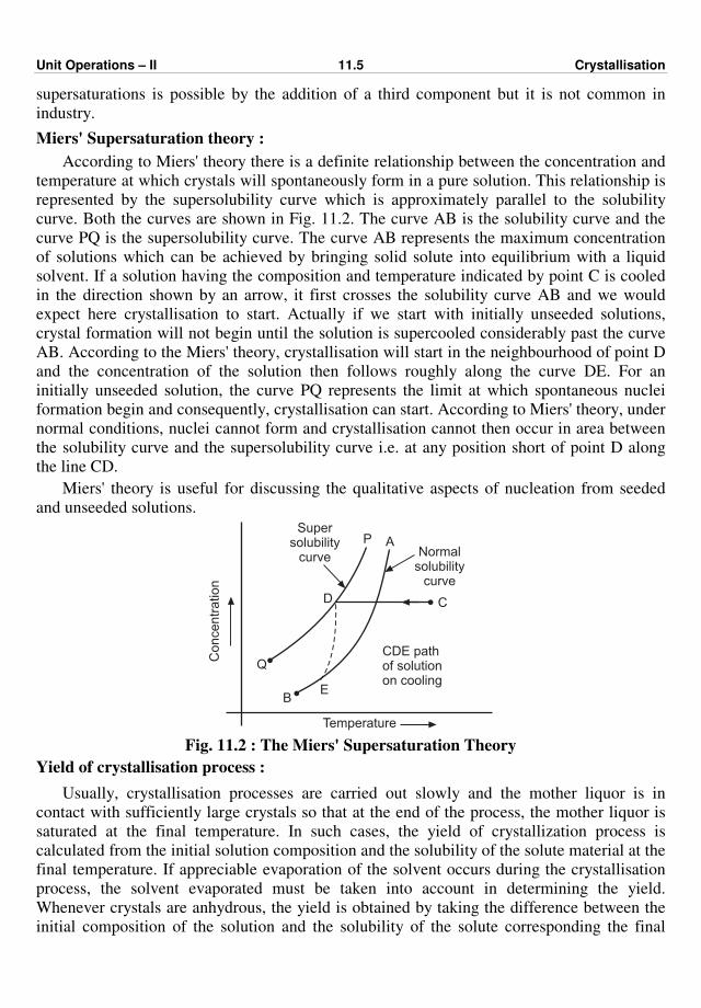
Unit Operations – II 11.5 Crystallisation
supersaturations is possible by the addition of a third component but it is not common in
industry.
Miers' Supersaturation theory :
According to Miers' theory there is a definite relationship between the concentration and
temperature at which crystals will spontaneously form in a pure solution. This relationship is
represented by the supersolubility curve which is approximately parallel to the solubility
curve. Both the curves are shown in Fig. 11.2. The curve AB is the solubility curve and the
curve PQ is the supersolubility curve. The curve AB represents the maximum concentration
of solutions which can be achieved by bringing solid solute into equilibrium with a liquid
solvent. If a solution having the composition and temperature indicated by point C is cooled
in the direction shown by an arrow, it first crosses the solubility curve AB and we would
expect here crystallisation to start. Actually if we start with initially unseeded solutions,
crystal formation will not begin until the solution is supercooled considerably past the curve
AB. According to the Miers' theory, crystallisation will start in the neighbourhood of point D
and the concentration of the solution then follows roughly along the curve DE. For an
initially unseeded solution, the curve PQ represents the limit at which spontaneous nuclei
formation begin and consequently, crystallisation can start. According to Miers' theory, under
normal conditions, nuclei cannot form and crystallisation cannot then occur in area between
the solubility curve and the supersolubility curve i.e. at any position short of point D along
the line CD.
Miers' theory is useful for discussing the qualitative aspects of nucleation from seeded
and unseeded solutions.
Concentr
ation
D
P A
Q
BE
Supersolubility
curve Normalsolubility
curve
C
CDE pathof solutionon cooling
Temperature
Fig. 11.2 : The Miers' Supersaturation Theory
Yield of crystallisation process :
Usually, crystallisation processes are carried out slowly and the mother liquor is in
contact with sufficiently large crystals so that at the end of the process, the mother liquor is
saturated at the final temperature. In such cases, the yield of crystallization process is
calculated from the initial solution composition and the solubility of the solute material at the
final temperature. If appreciable evaporation of the solvent occurs during the crystallisation
process, the solvent evaporated must be taken into account in determining the yield.
Whenever crystals are anhydrous, the yield is obtained by taking the difference between the
initial composition of the solution and the solubility of the solute corresponding the final
Unit Operations – II 11.6 Crystallisation
temperature of the process. In cases where material precipitates as a hydrated salt, we have to
take into account the water of crystallisation (in crystals), as this water is not available for
retaining solute in the solution. Under these circumstances, the key to the calculations of
yields is to express all the compositions in terms of hydrated salt and excess water (free
water), as the excess water remains constant during crystallisation operation and the
compositions or amounts thus expressed on the basis of excess water can be deducted in
order to obtain the correct results.
The percentage yield of a crystallisation process is the amount of the solute crystallised/
expressed as a percentage of the amount of the solute present in the feed solution.
Crystal form :
The constituent particles of a crystal are arranged in an orderly and repetitive manner.
The constituent particles may be atoms, molecules or ions. They are arranged in orderly three
dimensional arrays called space lattices. Crystals are classified according to the angle
between the faces and this is the area of the science of crystallography. Different forms of
crystals based upon the angle between faces and lengths of axes are : cubic, tetragonal,
orthorhombic, hexagonal, monoclinic, triclinic and trigonal.
Caking of Crystals :
Caking of crystalline materials is caused by a small amount of dissolution occuring at the
surface of crystals and subsequent re-evaporation of the solvent. Due to caking, the crystals
can get very tightly bonded together.
Since the vapour pressure of a saturated solution of a crystalline solid is less than that of
pure water at a given temperature, condensation can take place on the surface of the crystals
even though the atmospheric relative humidity is less than 100 percent. The solution thus
formed enters into/penetrates into the pack of crystals as a result of capillary action of the
small gaps between the crystals and caking can result due to subsequent evaporation of
moisture when the atmospheric humidity falls. Crystalline materials can also cake at a
constant relative humidity, as the vapour pressure of a solution is less in a small capillary as
compared to it in a large capillary as a result of temperature effect. As condensation occurs,
the small particles get first dissolved and therefore average size of capillaries increases and
the vapour pressure of the solution may increase sufficiently for evaporation to take place.
When the particle size is non-uniform, a crystalline material will cake more rapidly as the
porosity of a bed of particles of mixed sizes is less and fine particles are more readily
soluble. Thus, the tendency of crystalline materials to cake can be reduced by forming
crystals of relatively large and uniform sizes or by adding a water repellent agent, such as
stearic acid.
Magma : It is a two-phase mixture of mother liquor and crystals that occupies the
crystalliser and withdrawn as a product.
In order to reduce the load on a crystalliser, evaporation may be carried out to remove the
excess solvent from a solution. Crystallisation is generally followed by filtration for the
separation of crystals from the mother liquor.
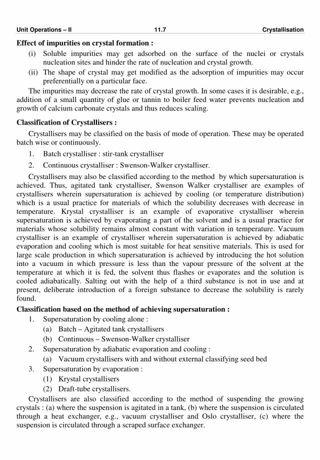
Unit Operations – II 11.7 Crystallisation
Effect of impurities on crystal formation :
(i) Soluble impurities may get adsorbed on the surface of the nuclei or crystals
nucleation sites and hinder the rate of nucleation and crystal growth.
(ii) The shape of crystal may get modified as the adsorption of impurities may occur
preferentially on a particular face.
The impurities may decrease the rate of crystal growth. In some cases it is desirable, e.g.,
addition of a small quantity of glue or tannin to boiler feed water prevents nucleation and
growth of calcium carbonate crystals and thus reduces scaling.
Classification of Crystallisers :
Crystallisers may be classified on the basis of mode of operation. These may be operated
batch wise or continuously.
1. Batch crystalliser : stir-tank crystalliser
2. Continuous crystalliser : Swenson-Walker crystalliser.
Crystallisers may also be classified according to the method by which supersaturation is
achieved. Thus, agitated tank crystalliser, Swenson Walker crystalliser are examples of
crystallisers wherein supersaturation is achieved by cooling (or temperature distribution)
which is a usual practice for materials of which the solubility decreases with decrease in
temperature. Krystal crystalliser is an example of evaporative crystalliser wherein
supersaturation is achieved by evaporating a part of the solvent and is a usual practice for
materials whose solubility remains almost constant with variation in temperature. Vacuum
crystalliser is an example of crystalliser wherein supersaturation is achieved by adiabatic
evaporation and cooling which is most suitable for heat sensitive materials. This is used for
large scale production in which supersaturation is achieved by introducing the hot solution
into a vacuum in which pressure is less than the vapour pressure of the solvent at the
temperature at which it is fed, the solvent thus flashes or evaporates and the solution is
cooled adiabatically. Salting out with the help of a third substance is not in use and at
present, deliberate introduction of a foreign substance to decrease the solubility is rarely
found.
Classification based on the method of achieving supersaturation :
1. Supersaturation by cooling alone :
(a) Batch – Agitated tank crystallisers
(b) Continuous – Swenson-Walker crystalliser
2. Supersaturation by adiabatic evaporation and cooling :
(a) Vacuum crystallisers with and without external classifying seed bed
3. Supersaturation by evaporation :
(1) Krystal crystallisers
(2) Draft-tube crystallisers.
Crystallisers are also classified according to the method of suspending the growing
crystals : (a) where the suspension is agitated in a tank, (b) where the suspension is circulated
through a heat exchanger, e.g., vacuum crystalliser and Oslo crystalliser, (c) where the
suspension is circulated through a scraped surface exchanger.
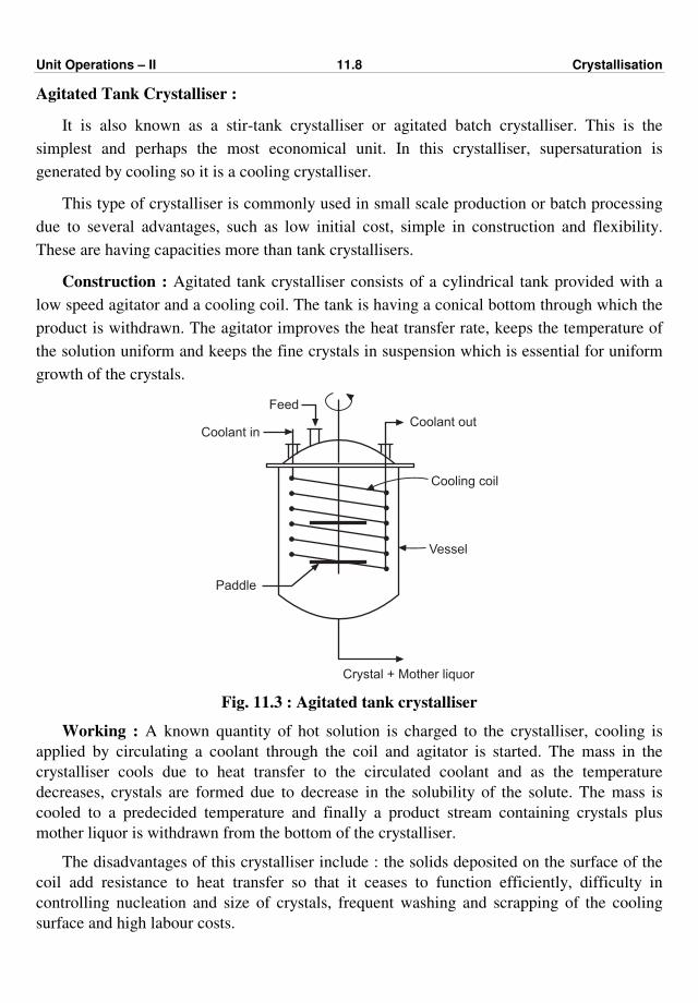
Unit Operations – II 11.8 Crystallisation
Agitated Tank Crystalliser :
It is also known as a stir-tank crystalliser or agitated batch crystalliser. This is the
simplest and perhaps the most economical unit. In this crystalliser, supersaturation is
generated by cooling so it is a cooling crystalliser.
This type of crystalliser is commonly used in small scale production or batch processing
due to several advantages, such as low initial cost, simple in construction and flexibility.
These are having capacities more than tank crystallisers.
Construction : Agitated tank crystalliser consists of a cylindrical tank provided with a
low speed agitator and a cooling coil. The tank is having a conical bottom through which the
product is withdrawn. The agitator improves the heat transfer rate, keeps the temperature of
the solution uniform and keeps the fine crystals in suspension which is essential for uniform
growth of the crystals.
Feed
Coolant inCoolant out
Cooling coil
Paddle
Vessel
Crystal + Mother liquor
Fig. 11.3 : Agitated tank crystalliser
Working : A known quantity of hot solution is charged to the crystalliser, cooling is
applied by circulating a coolant through the coil and agitator is started. The mass in the
crystalliser cools due to heat transfer to the circulated coolant and as the temperature
decreases, crystals are formed due to decrease in the solubility of the solute. The mass is
cooled to a predecided temperature and finally a product stream containing crystals plus
mother liquor is withdrawn from the bottom of the crystalliser.
The disadvantages of this crystalliser include : the solids deposited on the surface of the
coil add resistance to heat transfer so that it ceases to function efficiently, difficulty in
controlling nucleation and size of crystals, frequent washing and scrapping of the cooling
surface and high labour costs.
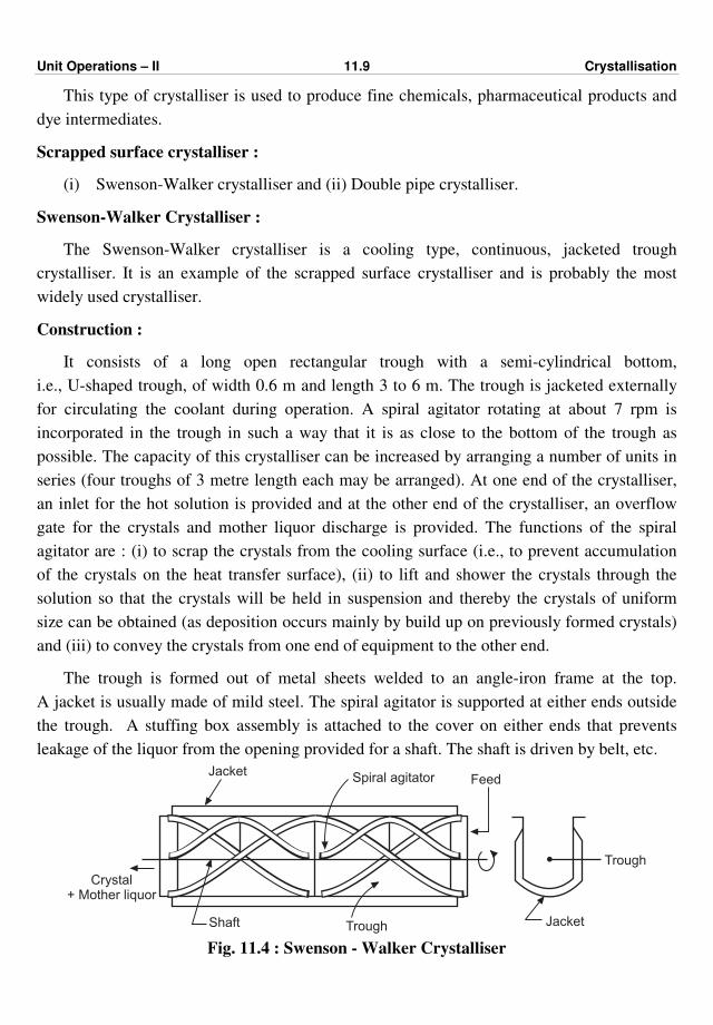
Unit Operations – II 11.9 Crystallisation
This type of crystalliser is used to produce fine chemicals, pharmaceutical products and
dye intermediates.
Scrapped surface crystalliser :
(i) Swenson-Walker crystalliser and (ii) Double pipe crystalliser.
Swenson-Walker Crystalliser :
The Swenson-Walker crystalliser is a cooling type, continuous, jacketed trough
crystalliser. It is an example of the scrapped surface crystalliser and is probably the most
widely used crystalliser.
Construction :
It consists of a long open rectangular trough with a semi-cylindrical bottom,
i.e., U-shaped trough, of width 0.6 m and length 3 to 6 m. The trough is jacketed externally
for circulating the coolant during operation. A spiral agitator rotating at about 7 rpm is
incorporated in the trough in such a way that it is as close to the bottom of the trough as
possible. The capacity of this crystalliser can be increased by arranging a number of units in
series (four troughs of 3 metre length each may be arranged). At one end of the crystalliser,
an inlet for the hot solution is provided and at the other end of the crystalliser, an overflow
gate for the crystals and mother liquor discharge is provided. The functions of the spiral
agitator are : (i) to scrap the crystals from the cooling surface (i.e., to prevent accumulation
of the crystals on the heat transfer surface), (ii) to lift and shower the crystals through the
solution so that the crystals will be held in suspension and thereby the crystals of uniform
size can be obtained (as deposition occurs mainly by build up on previously formed crystals)
and (iii) to convey the crystals from one end of equipment to the other end.
The trough is formed out of metal sheets welded to an angle-iron frame at the top.
A jacket is usually made of mild steel. The spiral agitator is supported at either ends outside
the trough. A stuffing box assembly is attached to the cover on either ends that prevents
leakage of the liquor from the opening provided for a shaft. The shaft is driven by belt, etc.
Jacket
Trough
FeedSpiral agitatorJacket
Shaft
Crystal+ Mother liquor
Trough Fig. 11.4 : Swenson - Walker Crystalliser
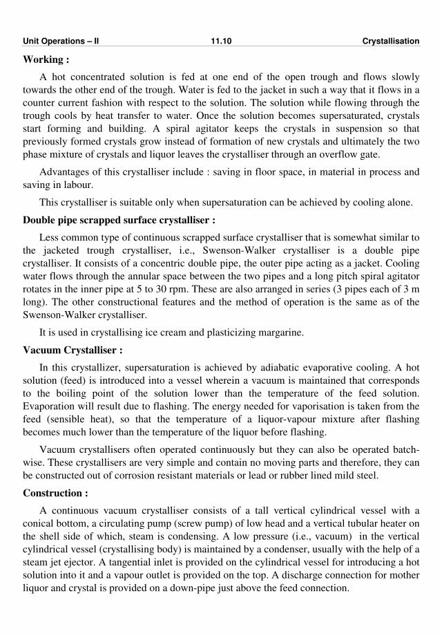
Unit Operations – II 11.10 Crystallisation
Working :
A hot concentrated solution is fed at one end of the open trough and flows slowly
towards the other end of the trough. Water is fed to the jacket in such a way that it flows in a
counter current fashion with respect to the solution. The solution while flowing through the
trough cools by heat transfer to water. Once the solution becomes supersaturated, crystals
start forming and building. A spiral agitator keeps the crystals in suspension so that
previously formed crystals grow instead of formation of new crystals and ultimately the two
phase mixture of crystals and liquor leaves the crystalliser through an overflow gate.
Advantages of this crystalliser include : saving in floor space, in material in process and
saving in labour.
This crystalliser is suitable only when supersaturation can be achieved by cooling alone.
Double pipe scrapped surface crystalliser :
Less common type of continuous scrapped surface crystalliser that is somewhat similar to
the jacketed trough crystalliser, i.e., Swenson-Walker crystalliser is a double pipe
crystalliser. It consists of a concentric double pipe, the outer pipe acting as a jacket. Cooling
water flows through the annular space between the two pipes and a long pitch spiral agitator
rotates in the inner pipe at 5 to 30 rpm. These are also arranged in series (3 pipes each of 3 m
long). The other constructional features and the method of operation is the same as of the
Swenson-Walker crystalliser.
It is used in crystallising ice cream and plasticizing margarine.
Vacuum Crystalliser :
In this crystallizer, supersaturation is achieved by adiabatic evaporative cooling. A hot
solution (feed) is introduced into a vessel wherein a vacuum is maintained that corresponds
to the boiling point of the solution lower than the temperature of the feed solution.
Evaporation will result due to flashing. The energy needed for vaporisation is taken from the
feed (sensible heat), so that the temperature of a liquor-vapour mixture after flashing
becomes much lower than the temperature of the liquor before flashing.
Vacuum crystallisers often operated continuously but they can also be operated batch-
wise. These crystallisers are very simple and contain no moving parts and therefore, they can
be constructed out of corrosion resistant materials or lead or rubber lined mild steel.
Construction :
A continuous vacuum crystalliser consists of a tall vertical cylindrical vessel with a
conical bottom, a circulating pump (screw pump) of low head and a vertical tubular heater on
the shell side of which, steam is condensing. A low pressure (i.e., vacuum) in the vertical
cylindrical vessel (crystallising body) is maintained by a condenser, usually with the help of a
steam jet ejector. A tangential inlet is provided on the cylindrical vessel for introducing a hot
solution into it and a vapour outlet is provided on the top. A discharge connection for mother
liquor and crystal is provided on a down-pipe just above the feed connection.
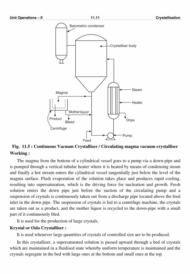
Unit Operations – II 11.11 Crystallisation
Barometric condenser
Crystalliser body
Steam
Heater
Drips
Pump
Product
Magma
Motherliquor
Bleed
Centrifuge
Feed
Fig. 11.5 : Continuous Vacuum Crystalliser / Circulating magma vacuum crystalliser
Working :
The magma from the bottom of a cylindrical vessel goes to a pump via a down-pipe and
is pumped through a vertical tubular heater where it is heated by means of condensing steam
and finally a hot stream enters the cylindrical vessel tangentially just below the level of the
magma surface. Flash evaporation of the solution takes place and produces rapid cooling,
resulting into supersaturation, which is the driving force for nucleation and growth. Fresh
solution enters the down pipe just before the suction of the circulating pump and a
suspension of crystals is continuously taken out from a discharge pipe located above the feed
inlet in the down pipe. The suspension of crystals is fed to a centrifuge machine, the crystals
are taken out as a product, and the mother liquor is recycled to the down-pipe with a small
part of it continuously bled.
It is used for the production of large crystals.
Krystal or Oslo Crystalliser :
It is used whenever large quantities of crystals of controlled size are to be produced.
In this crystalliser, a supersaturated solution is passed upward through a bed of crystals
which are maintained in a fluidised state whereby uniform temperature is maintained and the
crystals segregate in the bed with large ones at the bottom and small ones at the top.
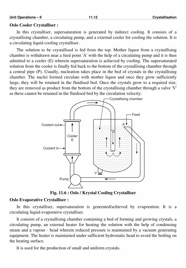
Unit Operations – II 11.12 Crystallisation
Oslo Cooler Crystalliser :
In this crystalliser, supersaturation is generated by indirect cooling. It consists of a
crystallising chamber, a circulating pump, and a external cooler for cooling the solution. It is
a circulating liquid cooling crystalliser.
The solution to be crystallised is fed from the top. Mother liquor from a crystallising
chamber is withdrawn near a feed point 'A' with the help of a circulating pump and it is then
admitted to a cooler (E) wherein supersaturation is achieved by cooling. The supersaturated
solution from the cooler is finally fed back to the bottom of the crystallising chamber through
a central pipe (P). Usually, nucleation takes place in the bed of crystals in the crystallising
chamber. The nuclei formed circulate with mother liquor and once they grow sufficiently
large, they will be retained in the fluidised bed. Once the crystals grow to a required size,
they are removed as product from the bottom of the crystallising chamber through a valve 'V'
as these cannot be retained in the fluidised bed by the circulation velocity.
V
Feed
A
Crystallising chamber
Coolant out
Coolant in
CoolerE
Pump
P
Fig. 11.6 : Oslo / Krystal Cooling Crystalliser
Oslo Evaporative Crystalliser :
In this crystalliser, supersaturation is generated/achieved by evaporation. It is a
circulating liquid evaporative crystalliser.
It consists of a crystallising chamber containing a bed of forming and growing crystals, a
circulating pump, an external heater for heating the solution with the help of condensing
steam and a vapour - head wherein reduced pressure is maintained by a vacuum generating
equipment. The heater is maintained under sufficient hydrostatic head to avoid the boiling on
the heating surface.
It is used for the production of small and uniform crystals.
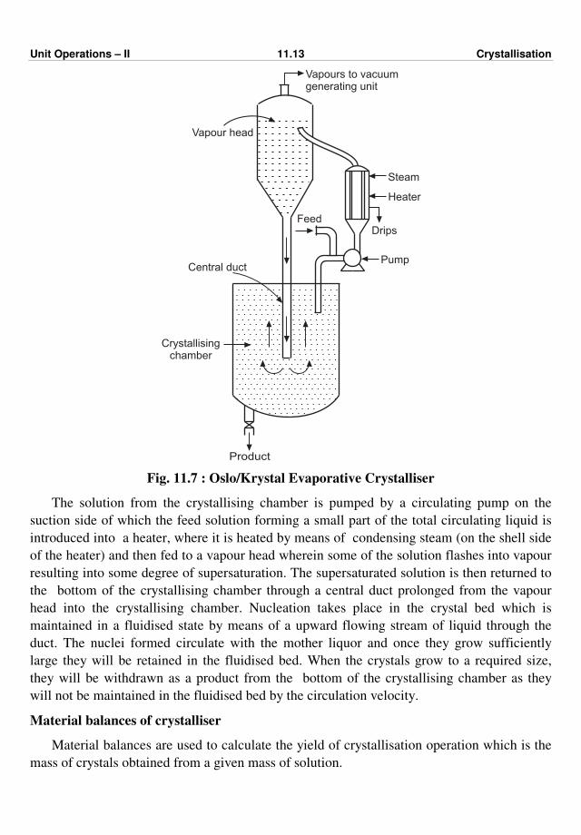
Unit Operations – II 11.13 Crystallisation
Product
Vapour head
Steam
Heater
DripsFeed
Vapours to vacuumgenerating unit
PumpCentral duct
Crystallisingchamber
Fig. 11.7 : Oslo/Krystal Evaporative Crystalliser
The solution from the crystallising chamber is pumped by a circulating pump on the
suction side of which the feed solution forming a small part of the total circulating liquid is
introduced into a heater, where it is heated by means of condensing steam (on the shell side
of the heater) and then fed to a vapour head wherein some of the solution flashes into vapour
resulting into some degree of supersaturation. The supersaturated solution is then returned to
the bottom of the crystallising chamber through a central duct prolonged from the vapour
head into the crystallising chamber. Nucleation takes place in the crystal bed which is
maintained in a fluidised state by means of a upward flowing stream of liquid through the
duct. The nuclei formed circulate with the mother liquor and once they grow sufficiently
large they will be retained in the fluidised bed. When the crystals grow to a required size,
they will be withdrawn as a product from the bottom of the crystallising chamber as they
will not be maintained in the fluidised bed by the circulation velocity.
Material balances of crystalliser
Material balances are used to calculate the yield of crystallisation operation which is the
mass of crystals obtained from a given mass of solution.
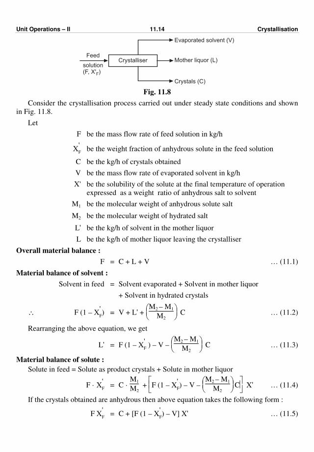
Unit Operations – II 11.14 Crystallisation
Feed
solution(F, X' )F
Evaporated solvent (V)
Mother liquor (L)
Crystals (C)
Crystalliser
Fig. 11.8
Consider the crystallisation process carried out under steady state conditions and shown
in Fig. 11.8.
Let
F be the mass flow rate of feed solution in kg/h
X'F be the weight fraction of anhydrous solute in the feed solution
C be the kg/h of crystals obtained
V be the mass flow rate of evaporated solvent in kg/h
X' be the solubility of the solute at the final temperature of operation
expressed as a weight ratio of anhydrous salt to solvent
M1 be the molecular weight of anhydrous solute salt
M2 be the molecular weight of hydrated salt
L' be the kg/h of solvent in the mother liquor
L be the kg/h of mother liquor leaving the crystalliser
Overall material balance :
F = C + L + V … (11.1)
Material balance of solvent :
Solvent in feed = Solvent evaporated + Solvent in mother liquor
+ Solvent in hydrated crystals
∴ F (1 – X'F) = V + L' +
M2 – M1
M2 C … (11.2)
Rearranging the above equation, we get
L' = F (1 – X'F ) – V –
M2 – M1
M2 C … (11.3)
Material balance of solute :
Solute in feed = Solute as product crystals + Solute in mother liquor
F · X'F = C ·
M1
M2 +
F (1 – X'F) – V –
M2 – M1
M2 C X' … (11.4)
If the crystals obtained are anhydrous then above equation takes the following form :
F X'F = C + [F (1 – X
'F) – V] X' … (11.5)
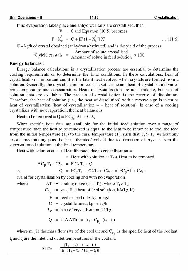
Unit Operations – II 11.15 Crystallisation
If no evaporation takes place and anhydrous salts are crystallised, then
V = 0 and Equation (10.5) becomes
F · X'F = C + [F (1 – X
'F)] X' … (11.6)
C – kg/h of crystal obtained (anhydrous/hydrated) and is the yield of the process.
% yield crystals = Amount of solute crystallised
Amount of solute in feed solution × 100
Energy balances :
Energy balance calculations in a crystallisation process are essential to determine the
cooling requirements or to determine the final conditions. In these calculations, heat of
crystallisation is important and it is the latent heat evolved when crystals are formed from a
solution. Generally, the crystallisation process is exothermic and heat of crystallisation varies
with temperature and concentration. Heats of crystallisation are not available, but heat of
solution data are available. The process of crystallisation is the reverse of dissolution.
Therefore, the heat of solution (i.e., the heat of dissolution) with a reverse sign is taken as
heat of crystallisation (heat of crystallisation = – heat of solution). In case of a cooling
crystalliser with no evaporation, the heat balance is
Heat to be removed = Q = F CpF ∆T + C λc
When specific heat data are available for the initial feed solution over a range of
temperature, then the heat to be removed is equal to the heat to be removed to cool the feed
from the initial temperature (T1) to the final temperature (T2, such that T1 > T2) without any
crystal precipitating plus the heat liberated/evolved due to formation of crystals from the
supersaturated solution at the final temperature.
Heat with solution at T1 + Heat liberated due to crystallisation =
= Heat with solution at T2 + Heat to be removed
F Cp T1 + Cλc = F Cp T2 + Q
∴ Q = FCpT1 – FCpT2 + CλC = FCp∆T + CλC
(valid for crystallisation by cooling and with no evaporation)
where ∆T = cooling range (T1 – T2), where T1 > T2
CpF = specified heat of feed solution, kJ/(kg·K)
F = feed or feed rate, kg or kg/h
C = crystal formed, kg or kg/h
λC = heat of crystallisation, kJ/kg
Q = U A ∆Tlm = .
m c · Cpc (t2 – t1)
where .
m c is the mass flow rate of the coolant and Cpc is the specific heat of the coolant,
t1 and t2 are the inlet and outlet temperatures of the coolant.
∆Tlm = (T1 – t2) – (T2 – t1)
ln [(T1 – t2) / (T2 – t1)]
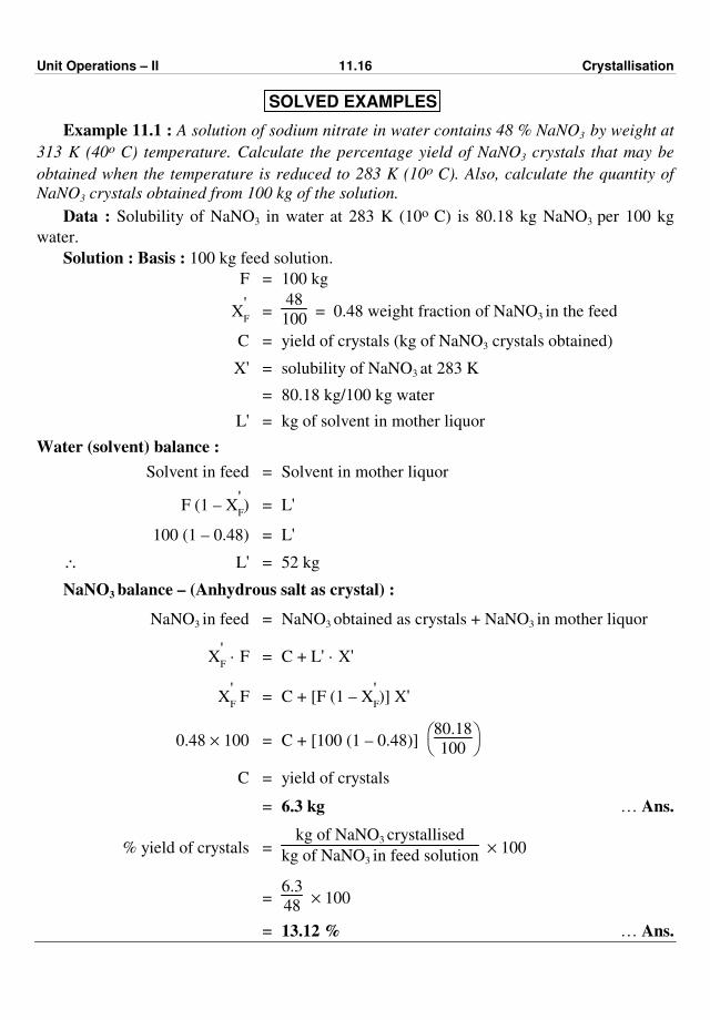
Unit Operations – II 11.16 Crystallisation
SOLVED EXAMPLES
Example 11.1 : A solution of sodium nitrate in water contains 48 % NaNO3 by weight at
313 K (40o C) temperature. Calculate the percentage yield of NaNO3 crystals that may be
obtained when the temperature is reduced to 283 K (10o C). Also, calculate the quantity of
NaNO3 crystals obtained from 100 kg of the solution.
Data : Solubility of NaNO3 in water at 283 K (10o C) is 80.18 kg NaNO3 per 100 kg
water.
Solution : Basis : 100 kg feed solution.
F = 100 kg
X'F =
48
100 = 0.48 weight fraction of NaNO3 in the feed
C = yield of crystals (kg of NaNO3 crystals obtained)
X' = solubility of NaNO3 at 283 K
= 80.18 kg/100 kg water
L' = kg of solvent in mother liquor
Water (solvent) balance :
Solvent in feed = Solvent in mother liquor
F (1 – X'F) = L'
100 (1 – 0.48) = L'
∴ L' = 52 kg
NaNO3 balance – (Anhydrous salt as crystal) :
NaNO3 in feed = NaNO3 obtained as crystals + NaNO3 in mother liquor
X'F · F = C + L' · X'
X'F F = C + [F (1 – X
'F)] X'
0.48 × 100 = C + [100 (1 – 0.48)]
80.18
100
C = yield of crystals
= 6.3 kg … Ans.
% yield of crystals = kg of NaNO3 crystallised
kg of NaNO3 in feed solution × 100
= 6.3
48 × 100
= 13.12 % … Ans.
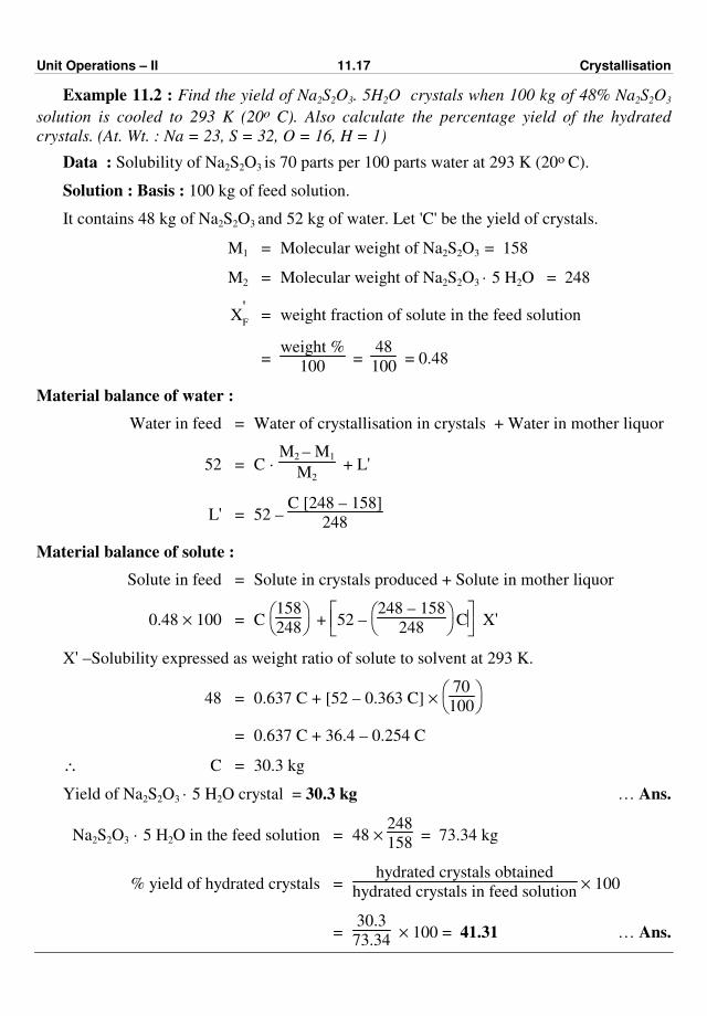
Unit Operations – II 11.17 Crystallisation
Example 11.2 : Find the yield of Na2S2O3. 5H2O crystals when 100 kg of 48% Na2S2O3
solution is cooled to 293 K (20o C). Also calculate the percentage yield of the hydrated
crystals. (At. Wt. : Na = 23, S = 32, O = 16, H = 1)
Data : Solubility of Na2S2O3 is 70 parts per 100 parts water at 293 K (20o C).
Solution : Basis : 100 kg of feed solution.
It contains 48 kg of Na2S2O3 and 52 kg of water. Let 'C' be the yield of crystals.
M1 = Molecular weight of Na2S2O3 = 158
M2 = Molecular weight of Na2S2O3 · 5 H2O = 248
X'F = weight fraction of solute in the feed solution
= weight %
100 =
48
100 = 0.48
Material balance of water :
Water in feed = Water of crystallisation in crystals + Water in mother liquor
52 = C · M2 – M1
M2 + L'
L' = 52 – C [248 – 158]
248
Material balance of solute :
Solute in feed = Solute in crystals produced + Solute in mother liquor
0.48 × 100 = C
158
248 +
52 –
248 – 158
248 C X'
X' –Solubility expressed as weight ratio of solute to solvent at 293 K.
48 = 0.637 C + [52 – 0.363 C] ×
70
100
= 0.637 C + 36.4 – 0.254 C
∴ C = 30.3 kg
Yield of Na2S2O3 · 5 H2O crystal = 30.3 kg … Ans.
Na2S2O3 · 5 H2O in the feed solution = 48 × 248
158 = 73.34 kg
% yield of hydrated crystals = hydrated crystals obtained
hydrated crystals in feed solution × 100
= 30.3
73.34 × 100 = 41.31 … Ans.
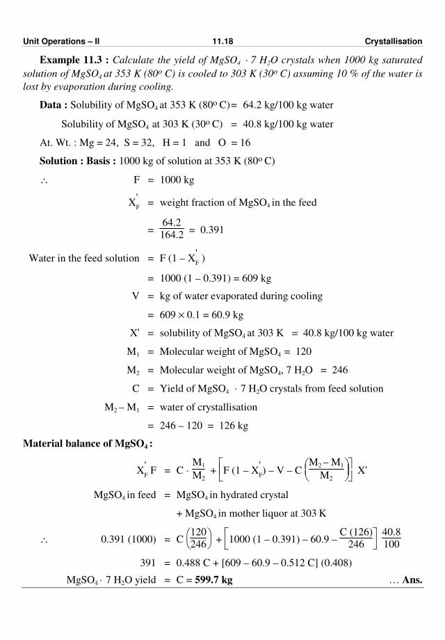
Unit Operations – II 11.18 Crystallisation
Example 11.3 : Calculate the yield of MgSO4 · 7 H2O crystals when 1000 kg saturated
solution of MgSO4 at 353 K (80o C) is cooled to 303 K (30o C) assuming 10 % of the water is
lost by evaporation during cooling.
Data : Solubility of MgSO4 at 353 K (80o C) = 64.2 kg/100 kg water
Solubility of MgSO4 at 303 K (30o C) = 40.8 kg/100 kg water
At. Wt. : Mg = 24, S = 32, H = 1 and O = 16
Solution : Basis : 1000 kg of solution at 353 K (80o C)
∴ F = 1000 kg
X'F = weight fraction of MgSO4 in the feed
= 64.2
164.2 = 0.391
Water in the feed solution = F (1 – X'F )
= 1000 (1 – 0.391) = 609 kg
V = kg of water evaporated during cooling
= 609 × 0.1 = 60.9 kg
X' = solubility of MgSO4 at 303 K = 40.8 kg/100 kg water
M1 = Molecular weight of MgSO4 = 120
M2 = Molecular weight of MgSO4, 7 H2O = 246
C = Yield of MgSO4 · 7 H2O crystals from feed solution
M2 – M1 = water of crystallisation
= 246 – 120 = 126 kg
Material balance of MgSO4 :
X'F F = C ·
M1
M2 +
F (1 – X'F) – V – C
M2 – M1
M2 X'
MgSO4 in feed = MgSO4 in hydrated crystal
+ MgSO4 in mother liquor at 303 K
∴ 0.391 (1000) = C
120
246 +
1000 (1 – 0.391) – 60.9 – C (126)
246
40.8
100
391 = 0.488 C + [609 – 60.9 – 0.512 C] (0.408)
MgSO4 · 7 H2O yield = C = 599.7 kg … Ans.

Unit Operations – II 11.19 Crystallisation
Example 11.4 : A hot solution containing 25 % by weight Na2CO3 is cooled to
293 K (20 oC) and crystals of Na2CO3 · 10 H2O are precipitated. At 293 K (20 oC), the
solubility is 21.5 kg anhydrous Na2CO3 per 100 kg of total water. Calculate the yield of
hydrated Na2CO3 crystals obtained if 5 % of the original water in the system evaporates on
cooling and the quantity of mother liquor based on 5000 kg of the hot solution.
At. Wt. : Na = 23, C = 12, O = 16, H = 1.
Solution : Basis : 5000 kg of hot solution of Na2CO3.
It contains :
Na2CO3 = 0.25 × 5000 = 1250 kg
Water = 0.75 × 5000 = 3750 kg
M1 = Mol. Wt. of Na2CO3 = 106
M2 = Mol. Wt. of Na2CO3 · 10 H2O = 286
M2 – M1 = water of crystallisation = 10 H2O = 180
∴ F = 5000 kg
X'F = weight fraction of Na2CO3 in the feed solution
= 25
100 = 0.25
Given : 5% of water is evaporated. Therefore,
V = kg of water evaporated during cooling
= 0.05 × 3750 = 187.5 kg
Material balance of water :
Water in feed = Water of crystallisation
+ Water in mother liquor + Water evaporated
0.75 (5000) = C
M2 – M1
M2 + L' + 187.5
3750 = C
286 – 106
286 + L' + 187.5
3562.5 = C
180
286 + L'
L' = 3562.5 – C
180
286
Material balance of solute :
Solute in feed = Solute in crystals produced + Solute in mother liquor
X'F F = C
M1
M2 + L' X'
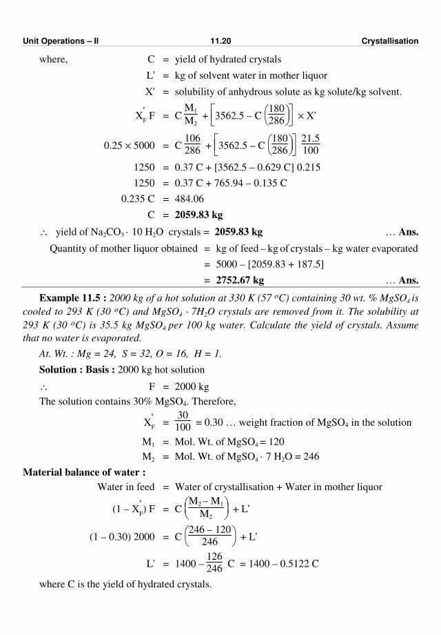
Unit Operations – II 11.20 Crystallisation
where, C = yield of hydrated crystals
L' = kg of solvent water in mother liquor
X' = solubility of anhydrous solute as kg solute/kg solvent.
X'F F = C
M1
M2 +
3562.5 – C
180
286 × X'
0.25 × 5000 = C 106
286 +
3562.5 – C
180
286
21.5
100
1250 = 0.37 C + [3562.5 – 0.629 C] 0.215
1250 = 0.37 C + 765.94 – 0.135 C
0.235 C = 484.06
C = 2059.83 kg
∴ yield of Na2CO3 · 10 H2O crystals = 2059.83 kg … Ans.
Quantity of mother liquor obtained = kg of feed – kg of crystals – kg water evaporated
= 5000 – [2059.83 + 187.5]
= 2752.67 kg … Ans.
Example 11.5 : 2000 kg of a hot solution at 330 K (57 oC) containing 30 wt. % MgSO4 is
cooled to 293 K (30 oC) and MgSO4 · 7H2O crystals are removed from it. The solubility at
293 K (30 oC) is 35.5 kg MgSO4 per 100 kg water. Calculate the yield of crystals. Assume
that no water is evaporated.
At. Wt. : Mg = 24, S = 32, O = 16, H = 1.
Solution : Basis : 2000 kg hot solution
∴ F = 2000 kg
The solution contains 30% MgSO4. Therefore,
X'F =
30
100 = 0.30 … weight fraction of MgSO4 in the solution
M1 = Mol. Wt. of MgSO4 = 120
M2 = Mol. Wt. of MgSO4 · 7 H2O = 246
Material balance of water :
Water in feed = Water of crystallisation + Water in mother liquor
(1 – X'F) F = C
M2 – M1
M2 + L'
(1 – 0.30) 2000 = C
246 – 120
246 + L'
L' = 1400 – 126
246 C = 1400 – 0.5122 C
where C is the yield of hydrated crystals.
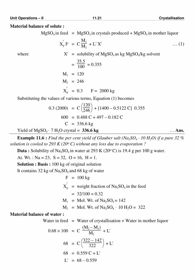
Unit Operations – II 11.21 Crystallisation
Material balance of solute :
MgSO4 in feed = MgSO4 in crystals produced + MgSO4 in mother liquor
X'F F = C
M1
M2 + L' X' … (1)
where X' = solubility of MgSO4 as kg MgSO4/kg solvent
= 35.5
100 = 0.355
M1 = 120
M2 = 246
X'F = 0.3 F = 2000 kg
Substituting the values of various terms, Equation (1) becomes
0.3 (2000) = C
120
246 + [1400 – 0.5122 C] 0.355
600 = 0.488 C + 497 – 0.182 C
C = 336.6 kg
Yield of MgSO4 · 7 H2O crystal = 336.6 kg … Ans.
Example 11.6 : Find the per cent yield of Glauber salt (Na2SO4 · 10 H2O) if a pure 32 %
solution is cooled to 293 K (20o C) without any loss due to evaporation ?
Data : Solubility of Na2SO4 in water at 293 K (20o C) is 19.4 g per 100 g water.
At. Wt. : Na = 23, S = 32, O = 16, H = 1.
Solution : Basis : 100 kg of original solution
It contains 32 kg of Na2SO4 and 68 kg of water
F = 100 kg
X'F = weight fraction of Na2SO4 in the feed
= 32/100 = 0.32
M1 = Mol. Wt. of Na2SO4 = 142
M2 = Mol. Wt. of Na2SO4 · 10 H2O = 322
Material balance of water :
Water in feed = Water of crystallisation + Water in mother liquor
0.68 × 100 = C (M2 – M1)
M2 + L'
68 = C
322 – 142
322 + L'
68 = 0.559 C + L'
L' = 68 – 0.559
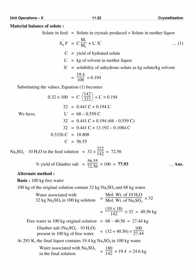
Unit Operations – II 11.22 Crystallisation
Material balance of solute :
Solute in feed = Solute in crystals produced + Solute in mother liquor
X'F F = C
M1
M2 + L' X' … (1)
C = yield of hydrated solute
L' = kg of solvent in mother liquor
X' = solubility of anhydrous solute as kg solute/kg solvent
= 19.4
100 = 0.194
Substituting the values, Equation (1) becomes
0.32 × 100 = C
142
322 + L' × 0.194
32 = 0.441 C + 0.194 L'
We have, L' = 68 – 0.559 C
32 = 0.441 C + 0.194 (68 – 0.559 C)
32 = 0.441 C + 13.192 – 0.1084 C
0.3326 C = 18.808
C = 56.55
Na2SO4 · 10 H2O in the feed solution = 32 × 322
142 = 72.56
% yield of Glauber salt = 56.55
72.56 × 100 = 77.93 … Ans.
Alternate method :
Basis : 100 kg free water
100 kg of the original solution contain 32 kg Na2SO4 and 68 kg water.
Water associated with
32 kg Na2SO4 in 100 kg solution = Mol. Wt. of 10 H2O
Mol. Wt. of Na2SO4 × 32
= (10 × 18)
142 × 32 = 40.56 kg
Free water in 100 kg original solution = 68 – 40.56 = 27.44 kg
Glauber salt (Na2SO4 · 10 H2O)
present in 100 kg of free water = (32 + 40.56) ×
100
27.44
At 293 K, the final liquor contains 19.4 kg Na2SO4 in 100 kg water.
Water associated with Na2SO4
in the final solution =
180
142 × 19.4 = 24.6 kg
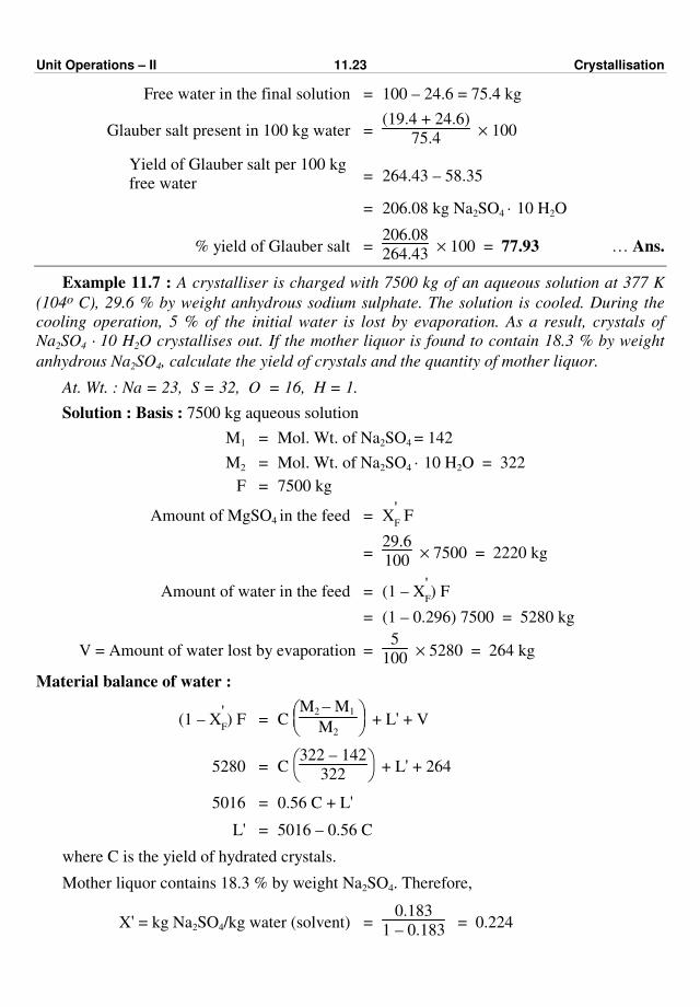
Unit Operations – II 11.23 Crystallisation
Free water in the final solution = 100 – 24.6 = 75.4 kg
Glauber salt present in 100 kg water = (19.4 + 24.6)
75.4 × 100
Yield of Glauber salt per 100 kg
free water = 264.43 – 58.35
= 206.08 kg Na2SO4 · 10 H2O
% yield of Glauber salt = 206.08
264.43 × 100 = 77.93 … Ans.
Example 11.7 : A crystalliser is charged with 7500 kg of an aqueous solution at 377 K
(104o C), 29.6 % by weight anhydrous sodium sulphate. The solution is cooled. During the
cooling operation, 5 % of the initial water is lost by evaporation. As a result, crystals of
Na2SO4 · 10 H2O crystallises out. If the mother liquor is found to contain 18.3 % by weight
anhydrous Na2SO4, calculate the yield of crystals and the quantity of mother liquor.
At. Wt. : Na = 23, S = 32, O = 16, H = 1.
Solution : Basis : 7500 kg aqueous solution
M1 = Mol. Wt. of Na2SO4 = 142
M2 = Mol. Wt. of Na2SO4 · 10 H2O = 322
F = 7500 kg
Amount of MgSO4 in the feed = X'F F
= 29.6
100 × 7500 = 2220 kg
Amount of water in the feed = (1 – X'F) F
= (1 – 0.296) 7500 = 5280 kg
V = Amount of water lost by evaporation = 5
100 × 5280 = 264 kg
Material balance of water :
(1 – X'F) F = C
M2 – M1
M2 + L' + V
5280 = C
322 – 142
322 + L' + 264
5016 = 0.56 C + L'
L' = 5016 – 0.56 C
where C is the yield of hydrated crystals.
Mother liquor contains 18.3 % by weight Na2SO4. Therefore,
X' = kg Na2SO4/kg water (solvent) = 0.183
1 – 0.183 = 0.224

Unit Operations – II 11.24 Crystallisation
Material balance of Na2SO4 :
X'F F = C
M1
M2 + L' X'
2220 = 142
322 C + 0.224 L'
2220 = 0.441 C + 0.224 L'
We have L' = 5016 – 0.56 C
∴ 2220 = 0.441 C + 0.224 (5016 – 0.56 C)
Solving, we get C = 3474.5 kg
Overall material balance :
Feed = Hydrated crystals + Mother liquor + Water evaporated
7500 = 3474.5 + Mother liquor + 264
∴ Amount of mother liquor = 3761.5 kg
Yield of Na2SO4 · 10 H2O crystals = 3474.5 kg … Ans.
Example 11.8 : A saturated solution of MgSO4 at 353 K (80o C) is cooled to 303 K
(30o C) in a crystalliser. During cooling, 4 % solution is lost by evaporation of water.
Estimate the quantity of the original saturated solution to be fed to the crystalliser per
1000 kg of MgSO4 · 7 H2O crystals.
Data : Solubility of MgSO4 at 303 K (30o C) = 40.8 kg/100 kg water
Solubility of MgSO4 at 353 K (80o C) = 64.2 kg/100 kg water
At. Wt. : Mg = 24, S = 32, O = 16, and H = 1.0
Solution : Basis : 100 kg of feed solution
M1 = Mol. Wt. of MgSO4 = 120
M2 = Mol. Wt. of Mg SO4 · 7 H2O = 246
M2 – M1 = Mol. Wt. of 7 H2O = 126
Solubility of MgSO4 at 353 K = 64.2 kg/100 kg water
Solubility of MgSO4 at 303 K = 40.8 kg/100 kg water
MgSO4 in the feed solution = 64.2
164.2 × 100 = 39.1 kg
Loss of solution by evaporation = 0.04 × 100 = 4 kg
Solute balance for hydrated salt :
F · X'F = C ·
M1
M2 +
F (1 – X'F) – V –
M2 – M1
M2 C X'
Unit Operations – II 11.25 Crystallisation
where F = 100 kg
X'F = 39.1/100 = 0.391
V = 4 kg
X' = 40.8
100 = 0.408
100 × 0.391 = 120
246 C +
100 (1 – 0.391) – 4 –
246 – 120
246 C × 0.408
39.1 = 0.4878 C + [60.9 – 4 – 0.512 C] × 0.408
0.2788 C = 15.89
C = 56.99 kg yield of crystals
C is the kg of hydrated crystals obtained.
For 56.99 kg of crystals, 100 kg of feed solution is required.
∴ For a yield of 1000 kg crystals‚
the charge to the crystalliser = 100
56.99 × 1000
(i.e., quantity of the feed solution) = 1754.56 kg … Ans.
Example 11.9 : A solution of sodium nitrate in water contains 48% NaNO3 by weight at
313 K temperature. Calculate the percentage yield of NaNO3 crystals that may be obtained
when temperature is reduced to 283 K. Solubility of NaNO3 at 283 K is 80.18 kg/100 kg
water.
Solution : Basis : 100 kg of feed solution.
Instead of using notation for various streams and the other terms as used before, we will
solve this problem by writing material balances and solving them simultaneously.
Let x be the kg of NaNO3 crystals obtained and y be the kg of mother liquor obtained.
Overall material balance :
Feed solution = crystals + mother liquor
100 = x + y … (1)
Feed solution contains 48% by weight NaNO3.
The solubility of NaNO3 at 283 K is 80.18 kg per 100 kg water.
It means that 180.18 kg (100 + 80.18) mother liquor contains 80.18 kg NaNO3.
Material balance of NaNO3 :
NaNO3 in feed solution = NaNO3 crystals + NaNO3 in mother liquor
0.48 × 100 = x + 80.18
180.18 y
48 = x + 0.445 y … (2)

Unit Operations – II 11.26 Crystallisation
Solving Equations (1) and (2) simultaneously gives
x + y = 100
x = 100 – y
48 = x + 0.445 y
48 = (100 – y) + 0.445 y
∴ 0.555 y = 52
y = 93.7 kg
x + 93.7 = 100
x = 6.3 kg
Yield of NaNO3 crystals from 100 kg solution = 6.3 kg
NaNO3 in the feed solution = 48 kg
% yield of NaNO3 crystals = 6.3
48 × 100
= 13.12 … Ans.
Note : You can adopt the same procedure to solve the previous problems.
Example 11.10 : Calculate the yield of MgSO4 · 7H2O crystals when 1000 kg saturated
solution of MgSO4 at 353 K is cooled to 303 K assuming 10% of water is lost by evaporation
during cooling.
Data : Solubility of MgSO4 at 353 K = 64.2 kg/100 kg water
Solubility of MgSO4 at 303 K = 40.8 kg/100 kg water
Mol. Wt. of MgSO4 = 120, Mol. Wt. of MgSO4 · 7 H2O = 246
Solution : Basis : 1000 kg of saturated solution at 353 K.
Let us solve this problem without using notation.
Let x be the kg of MgSO4 · 7 H2O crystals obtained, y be the kg of mother liquor
obtained.
Saturated solution = 1000 kg
Solubility at 353 K = 64.2 kg/100 kg water
i.e., 164.2 kg (100 + 64.2) of saturated solution contains 64.2 kg of MgSO4 and 100 kg of
water.
Water in the saturated solution = 100
164.2 × 1000
= 609 kg
MgSO4 in the saturated solution = 1000 – 609 = 391 kg
Water lost by evaporation = 10% of original water
Water lost by evaporation = 0.10 (609) = 60.9 kg
Unit Operations – II 11.27 Crystallisation
Overall material balance :
Feed solution = crystals + mother liquor + water lost by evaporation
1000 = x + y + 60.9
x + y = 939.1 … (1)
Solubility of MgSO4 at 303 K = 40.8 kg/100 kg water
i.e., 140.8 kg of mother liquor contains 40.8 kg of MgSO4 and 100 kg water.
We have :
1 kmol MgSO4 · 7H2O ≡ 1 kmol MgSO4
246 kg MgSO4 · 7H2O ≡ 120 kg MgSO4
i.e., 246 kg MgSO4 ⋅ 7H2 contain 120 kg MgSO4.
Material balance of MgSO4 :
MgSO4 in feed solution = MgSO4 in crystals + MgSO4 in mother liquor
391 = 120
246 × x +
40.8
140.8 y
391 = 0.488 x + 0.2898 y … (2)
Solving Equations (1) and (2) simultaneously gives
x + y = 939.1
y = 939.1 – x
391 = 0.488 x + 0.2898 (939.1 – x)
∴ x = 599.64 kg (crystals obtained)
599.64 + y = 939.1 ∴ y = 339.46 kg
Yield of MgSO4 · 7 H2O crystals = 599.64 kg … Ans.
EXERCISE
1. Fill in the blanks :
(a) ............ and ........... are the phases involved in crystallisation. Ans. Liquid, solid
(b) In crystallisation from solution, simultaneous ................ and mass transfer takes
place. Ans. heat
(c) In crystallisation, mass transfer occurs from the solution to ....... phase. Ans. solid
(d) ............... is the driving force for crystallisation. Ans. supersaturation
(e) For common salt (NaCl) ...... is independent of variation in temperature.
Ans. solubility
(f) Solubility is generally expressed as parts by weight ......... per ......... parts by weight
solvent. Ans. solute, 100
Unit Operations – II 11.28 Crystallisation
(g) For solutes whose solubility increases within increase in temperature, supersaturation
is achieved by .......... alone. Ans. cooling
(h) For solutes whose solubility remains more or less constant with temperature,
supersaturation is achieved by .......... of a part of the solvent. Ans. evaporation
(i) Vacuum crystalliser is used for ........... sensitive materials. Ans. heat
(j) ............ and crystal growth are the two basic steps in the overall process of
crystallisation. Ans. Nucleation.
2. Define the following terms :
(a) crystallisation (b) solubility (c) nucleation
(d) crystal growth (e) supersaturation.
3. Explain in brief solubility curves.
4. State various methods of generating supersaturation.
5. Give the classification of crystallisers.
6. Discuss in brief crystal formation.
7. Explain in brief with a neat sketch Swenson-Walker crystalliser.
8. Explain with a neat sketch Oslo-cooling crystalliser.
9. Draw a neat sketch of agitated tank crystalliser.
10. Draw a neat sketch of vacuum crystalliser and explain its construction.
ppp
(12.1)
CHAPTER TWELVE
DRYING
Drying refers to an operation in which the moisture of a substance (usually solid) is
removed by thermal means (i.e., with the help of thermal energy).
Drying usually refers to the removal of relatively small amounts of water from a solid or
nearly solid material. It involves the transfer of liquid from a wet solid into an unsaturated
gas phase (drying medium).
During drying operation, mass and heat transfer occur simultaneously. Heat is transferred
from the the bulk of the gas phase (drying medium) to the solid phase and mass is transferred
from the solid phase to the gas phase in the form of liquid and vapour through various
resistances. The material (liquid) that is transferred is the solute and transfer takes place as
the gas phase is always unsaturated with respect to the solute material.
In drying, relatively small amounts of water or other liquid is removed from a solid or
semi-solid material (using thermal energy), whereas in evaporation relatively large amount of
water is removed from solutions. Drying involves the removal of water at a temperature
below the boiling point, while evaporation involves the removal of water as vapour at its
boiling point. Drying involves circulation of a hot air or other gas over a solid material for
the removal of water, whereas evaporation involves use of steam heat for the removal of
water. To obtain products almost in the dried form is the purpose of drying operation, while
to obtain concentrated solutions is the main purpose of evaporation.
As the removal of moisture by thermal means is more costly than mechanical means
(e.g., filtration), the moisture content of material must be reduced to the minimum possible
level by the latter means before the material is fed to drying equipments.
In most of the drying operations, the heat (required to evaporate water) is provided by hot
air or any other gas-drying medium.
Drying is frequently the last operation in manufacturing processes and is usually carried
after evaporation, filtration, or crystallisation.
This operation is carried out in food, chemical, agricultural, pharmaceutical and textile
industries.
Drying operation is carried out for the reasons given below :
(i) For reducing the transport cost.
(ii) For purifying a crystalline product so that the solvent adhering to the crystals is
removed.
Unit Operations – II 12.2 Drying
(iii) For making a material more suitable for handling and storage. Handling and
storage of dry solids is easy.
(iv) To meet the market specifications of solid products set by the customers.
(v) For providing definite properties to materials.
(vi) In some cases for preventing corrosion arising due to the presence of moisture. Dry
chlorine gas is not corrosive but traces of moisture make it very corrosive.
(vii) Sometimes it is an essential part of the process (e.g., drying of paper in paper
making).
General Definitions :
The moisture content of a wet material may be expressed on the wet or dry basis.
Moisture content, wet basis :
The moisture content of a wet feed material, on wet basis, is defined as the ratio of the
weight of the moisture to the weight of the wet feed material. If X is the kg moisture
associated with one kg of dry solids, then
Moisture content (wet basis) = X
1 + X
The weight percent moisture of a wet feed material, on wet basis, is defined as the weight
of the moisture expressed as a percentage of the weight of the wet feed material (i.e., wet
solid).
Weight % moisture content (wet basis) = kg moisture
kg wet solid × 100 = 100
X
1 + X
Moisture content, dry basis :
The moisture of a wet feed material, on dry basis, is defined as the ratio of the weight of
the moisture to the weight of the dry solids present in the wet feed material. If the feed
material contains X kg moisture and 1 kg of dry solids, then
Moisture content (dry basis) = kg moisture
kg dry solid =
X
1 = X
Percentage moisture content on dry basis = 100 X
Equilibrium moisture content (X*) :
It is the moisture content of a substance that is in equilibrium with its vapour in the gas
phase under the specified humidity and temperature of the hot gas or air. It represents the
limiting moisture content to which a given material can be dried under constant drying
conditions.
It is the moisture content of a substance which is in equilibrium with a given partial
pressure of the vapour.
Bound Moisture content :
It is the moisture content in a material which exerts a vapour pressure less than that of
the pure liquid at the same temperature.
Unit Operations – II 12.3 Drying
Unbound moisture content :
It is the moisture held by a material in excess of the equilibrium moisture content
corresponding to saturation humidity. It is primarily held in the voids of solid.
It is the moisture content in a material which exerts an equilibrium vapour pressure
equal to that of the pure liquid at the same temperature.
Free moisture content :
It is the moisture contained by a material in excess of the equilibrium moisture content
(X – X*). At a given temperature and humidity, it is the moisture content of a material that
can be removed by drying. It may include bound and unbound moisture.
Critical moisture content :
It is the moisture content of a material at which the constant rate period ends and the
falling rate period starts. This moisture content is a function of constant drying rate, material
properties and particle size.
Constant rate period :
It is that part of the drying process during which the rate of drying expressed as the
moisture evaporated per unit time per unit area of drying surface remains constant.
Falling rate period :
It is that part of the drying process during which the rate of drying varies with time and
the instantaneous drying rate expressed as the amount of moisture evaporated per unit time
per unit area of drying surface continuously decreases.
Properties of air-water system :
The moisture removed (from a wet solid) during drying operation gets added in the hot
gas or air which in turn depends upon the temperature and humidity of the gas or air.
Usually, in drying operation the hot air is used as a drying medium, so it is essential to know
some of the properties of the air-water vapour system.
Relative humidity (R.H.) :
It is a measure of the degree of saturation of air at the dry bulb temperature.
It is defined as the ratio of the partial pressure of water vapour in the air water-vapour
mixture to the vapour pressure of pure water at the temperature of the mixture, expressed on
a percentage basis.
% R.H. = (pA/poA) × 100
where pA = partial pressure of water vapour in the mixture
poA = vapour pressure of pure water
when pA = poA, air is said to be saturated with water vapour.
The relative humidity is defined as the ratio of the actual water vapour content of air to
the water vapour content of the fully saturated air at the same temperature, expressed on a
percentage basis.

Unit Operations – II 12.4 Drying
Humidity (H)/Absolute humidity :
It is the ratio of the mass of water vapour to the mass of dry air present in the air-water
vapour mixture under any given set of conditions.
H = kg of water vapour
kg of dry air =
18
29
pA
P – pA = 0.62 Hm
Hm is the molal humidity.
Dry bulb temperature :
The temperature of the air-water vapour mixture recorded by a thermometer whose bulb
is kept dry is called dry bulb temperature.
Wet bulb temperature :
The temperature of the air-water vapour recorded by a thermometer whose bulb is kept
wet by wrapping a wet cloth in the open air is called wet bulb temperature.
Since the latent heat of vaporisation required for natural evaporation of water from the
cloth will be supplied from the bulb, the temperature of the bulb decreases. The evaporation
is continued until the air surrounding the bulb becomes saturated. Some of the heat will flow
from the surrounding air to the bulb by temperature difference, even then the temperature of
bulb will not rise as that heat gets consumed in evaporation of water. At one particular point,
the temperature becomes constant and is recorded as wet bulb temperature.
When the air is more unsaturated, then the difference between dry bulb temperature and
wet bulb temperature is more and is less for a more humid air. The relative humidity of the
air is found out from a psychrometric chart knowing wet bulb and dry bulb temperatures.
Saturation humidity :
It is the humidity of air when it is fully saturated with water vapour. It is denoted by the
symbol Hs.
Hs = 18
29 ( )p
oA/P – p
oA
Percentage humidity/Percentage saturation :
It is the ratio of the actual humidity (H) to the saturation humidity (Hs).
Percentage humidity = pA (P – poA )/p
oA (P – pA) × 100
Dew point :
When the air-water vapour mixture is cooled, at some temperature it becomes saturated
and further cooling results in the condensation of water vapour. The temperature at which
the condensation will first occur is known as dew point [i.e., it is temperature at which a
given air-water vapour mixture is saturated.] Dew point is lower or equal to the dry-bulb
temperature. For saturated air, the dew point, wet bulb and dry bulb temperatures are
identical.
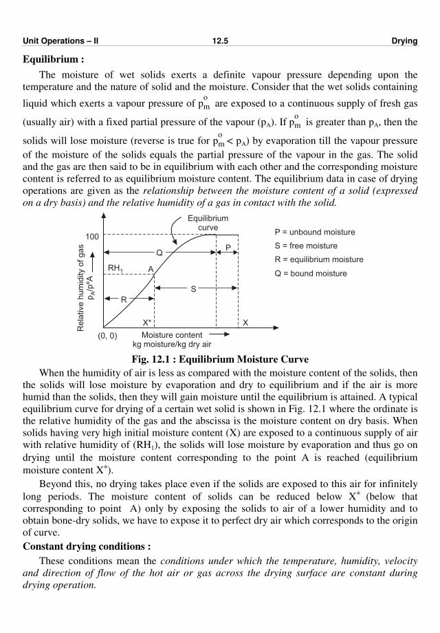
Unit Operations – II 12.5 Drying
Equilibrium :
The moisture of wet solids exerts a definite vapour pressure depending upon the
temperature and the nature of solid and the moisture. Consider that the wet solids containing
liquid which exerts a vapour pressure of po
m are exposed to a continuous supply of fresh gas
(usually air) with a fixed partial pressure of the vapour (pA). If po
m is greater than pA, then the
solids will lose moisture (reverse is true for po
m < pA) by evaporation till the vapour pressure
of the moisture of the solids equals the partial pressure of the vapour in the gas. The solid
and the gas are then said to be in equilibrium with each other and the corresponding moisture
content is referred to as equilibrium moisture content. The equilibrium data in case of drying
operations are given as the relationship between the moisture content of a solid (expressed
on a dry basis) and the relative humidity of a gas in contact with the solid.
PQ
S
R
RH1 A
P = unbound moisture
S = free moisture
R = equilibrium moisture
Q = bound moisture
X
(0, 0) Moisture contentkg moisture/kg dry air
Equilibriumcurve
100
X*
Rela
tive h
um
idity o
f gas
p/p
ºAA
Fig. 12.1 : Equilibrium Moisture Curve
When the humidity of air is less as compared with the moisture content of the solids, then
the solids will lose moisture by evaporation and dry to equilibrium and if the air is more
humid than the solids, then they will gain moisture until the equilibrium is attained. A typical
equilibrium curve for drying of a certain wet solid is shown in Fig. 12.1 where the ordinate is
the relative humidity of the gas and the abscissa is the moisture content on dry basis. When
solids having very high initial moisture content (X) are exposed to a continuous supply of air
with relative humidity of (RH1), the solids will lose moisture by evaporation and thus go on
drying until the moisture content corresponding to the point A is reached (equilibrium
moisture content X*).
Beyond this, no drying takes place even if the solids are exposed to this air for infinitely
long periods. The moisture content of solids can be reduced below X* (below that
corresponding to point A) only by exposing the solids to air of a lower humidity and to
obtain bone-dry solids, we have to expose it to perfect dry air which corresponds to the origin
of curve.
Constant drying conditions :
These conditions mean the conditions under which the temperature, humidity, velocity
and direction of flow of the hot air or gas across the drying surface are constant during
drying operation.
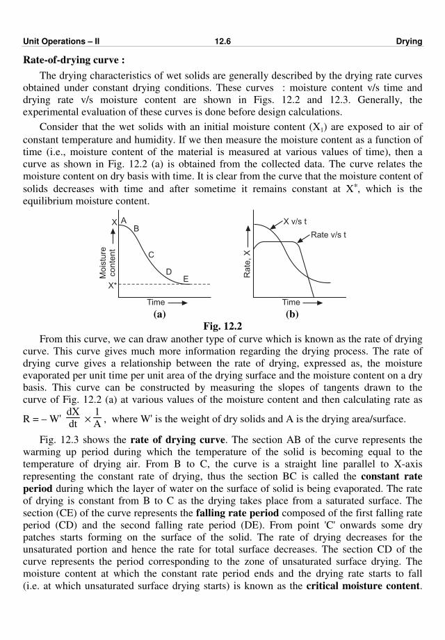
Unit Operations – II 12.6 Drying
Rate-of-drying curve :
The drying characteristics of wet solids are generally described by the drying rate curves
obtained under constant drying conditions. These curves : moisture content v/s time and
drying rate v/s moisture content are shown in Figs. 12.2 and 12.3. Generally, the
experimental evaluation of these curves is done before design calculations.
Consider that the wet solids with an initial moisture content (X1) are exposed to air of
constant temperature and humidity. If we then measure the moisture content as a function of
time (i.e., moisture content of the material is measured at various values of time), then a
curve as shown in Fig. 12.2 (a) is obtained from the collected data. The curve relates the
moisture content on dry basis with time. It is clear from the curve that the moisture content of
solids decreases with time and after sometime it remains constant at X*, which is the
equilibrium moisture content.
X AB
C
DE
X*
Mois
ture
conte
nt
Time Time
Rate
, X
X v/s t
Rate v/s t
(a) (b)
Fig. 12.2
From this curve, we can draw another type of curve which is known as the rate of drying
curve. This curve gives much more information regarding the drying process. The rate of
drying curve gives a relationship between the rate of drying, expressed as, the moisture
evaporated per unit time per unit area of the drying surface and the moisture content on a dry
basis. This curve can be constructed by measuring the slopes of tangents drawn to the
curve of Fig. 12.2 (a) at various values of the moisture content and then calculating rate as
R = – W' dX
dt ×
1
A , where W' is the weight of dry solids and A is the drying area/surface.
Fig. 12.3 shows the rate of drying curve. The section AB of the curve represents the
warming up period during which the temperature of the solid is becoming equal to the
temperature of drying air. From B to C, the curve is a straight line parallel to X-axis
representing the constant rate of drying, thus the section BC is called the constant rate
period during which the layer of water on the surface of solid is being evaporated. The rate
of drying is constant from B to C as the drying takes place from a saturated surface. The
section (CE) of the curve represents the falling rate period composed of the first falling rate
period (CD) and the second falling rate period (DE). From point 'C' onwards some dry
patches starts forming on the surface of the solid. The rate of drying decreases for the
unsaturated portion and hence the rate for total surface decreases. The section CD of the
curve represents the period corresponding to the zone of unsaturated surface drying. The
moisture content at which the constant rate period ends and the drying rate starts to fall
(i.e. at which unsaturated surface drying starts) is known as the critical moisture content.
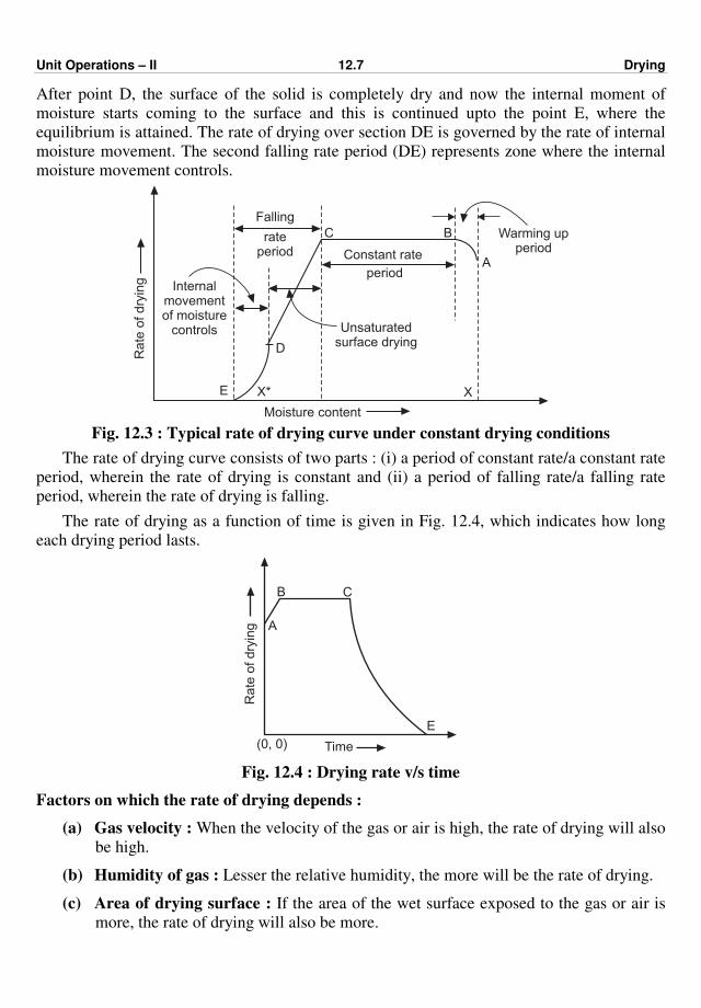
Unit Operations – II 12.7 Drying
After point D, the surface of the solid is completely dry and now the internal moment of
moisture starts coming to the surface and this is continued upto the point E, where the
equilibrium is attained. The rate of drying over section DE is governed by the rate of internal
moisture movement. The second falling rate period (DE) represents zone where the internal
moisture movement controls.
Ra
te o
f d
ryin
g
Moisture content
E X* X
D
Internalmovementof moisture
controls
Falling
rateperiod
C
Constant rate
period
B
A
Unsaturatedsurface drying
Warming upperiod
Fig. 12.3 : Typical rate of drying curve under constant drying conditions
The rate of drying curve consists of two parts : (i) a period of constant rate/a constant rate
period, wherein the rate of drying is constant and (ii) a period of falling rate/a falling rate
period, wherein the rate of drying is falling.
The rate of drying as a function of time is given in Fig. 12.4, which indicates how long
each drying period lasts.
Time
E
(0, 0)
Ra
te o
f d
ryin
g
B C
A
Fig. 12.4 : Drying rate v/s time
Factors on which the rate of drying depends :
(a) Gas velocity : When the velocity of the gas or air is high, the rate of drying will also
be high.
(b) Humidity of gas : Lesser the relative humidity, the more will be the rate of drying.
(c) Area of drying surface : If the area of the wet surface exposed to the gas or air is
more, the rate of drying will also be more.
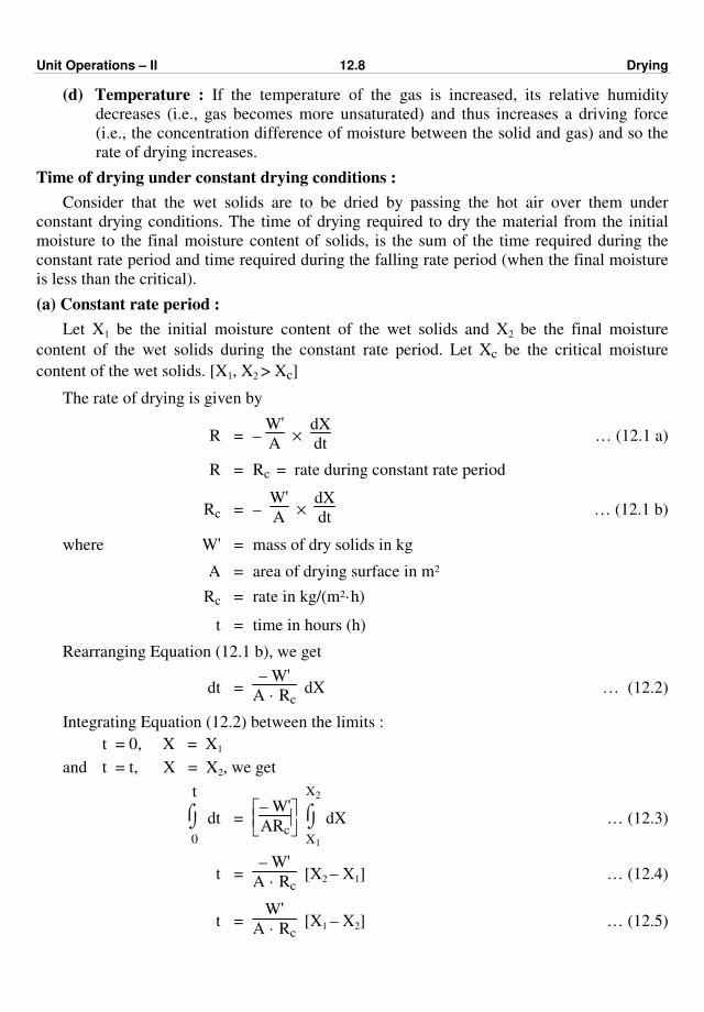
Unit Operations – II 12.8 Drying
(d) Temperature : If the temperature of the gas is increased, its relative humidity
decreases (i.e., gas becomes more unsaturated) and thus increases a driving force
(i.e., the concentration difference of moisture between the solid and gas) and so the
rate of drying increases.
Time of drying under constant drying conditions :
Consider that the wet solids are to be dried by passing the hot air over them under
constant drying conditions. The time of drying required to dry the material from the initial
moisture to the final moisture content of solids, is the sum of the time required during the
constant rate period and time required during the falling rate period (when the final moisture
is less than the critical).
(a) Constant rate period :
Let X1 be the initial moisture content of the wet solids and X2 be the final moisture
content of the wet solids during the constant rate period. Let Xc be the critical moisture
content of the wet solids. [X1, X2 > Xc]
The rate of drying is given by
R = – W'A
× dX
dt … (12.1 a)
R = Rc = rate during constant rate period
Rc = – W'A
× dX
dt … (12.1 b)
where W' = mass of dry solids in kg
A = area of drying surface in m2
Rc = rate in kg/(m2·h)
t = time in hours (h)
Rearranging Equation (12.1 b), we get
dt = – W'
A · Rc dX … (12.2)
Integrating Equation (12.2) between the limits :
t = 0, X = X1
and t = t, X = X2, we get
⌡⌠
0
t
dt =
– W'
ARc ⌡⌠
X1
X2
dX … (12.3)
t = – W'
A · Rc [X2 – X1] … (12.4)
t = W'
A · Rc [X1 – X2] … (12.5)
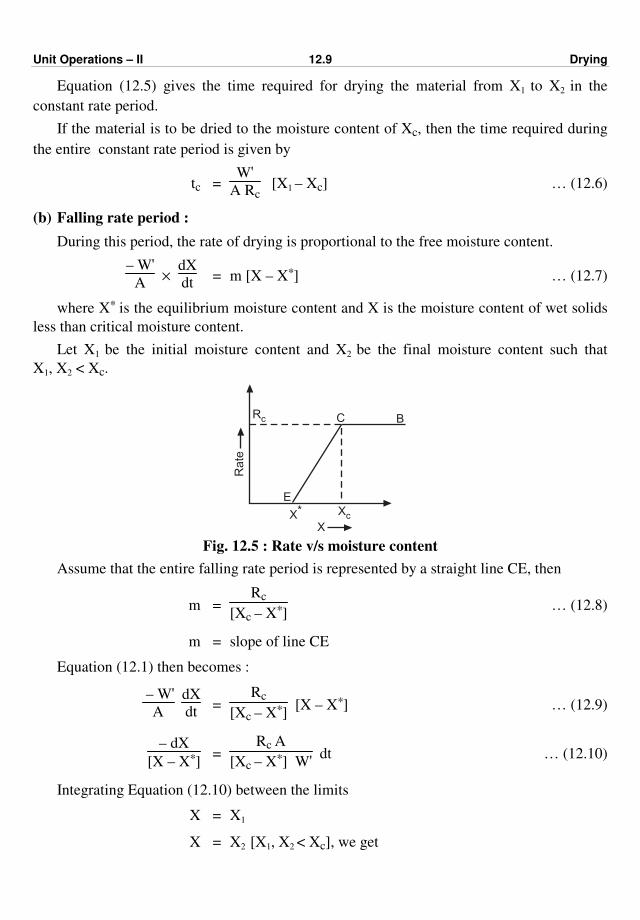
Unit Operations – II 12.9 Drying
Equation (12.5) gives the time required for drying the material from X1 to X2 in the
constant rate period.
If the material is to be dried to the moisture content of Xc, then the time required during
the entire constant rate period is given by
tc = W'
A Rc [X1 – Xc] … (12.6)
(b) Falling rate period :
During this period, the rate of drying is proportional to the free moisture content.
– W'
A ×
dX
dt = m [X – X*] … (12.7)
where X* is the equilibrium moisture content and X is the moisture content of wet solids
less than critical moisture content.
Let X1 be the initial moisture content and X2 be the final moisture content such that
X1, X2 < Xc.
E
XcX*
X
Ra
te
Rc C B
Fig. 12.5 : Rate v/s moisture content
Assume that the entire falling rate period is represented by a straight line CE, then
m = Rc
[Xc – X*] … (12.8)
m = slope of line CE
Equation (12.1) then becomes :
– W'
A
dX
dt =
Rc
[Xc – X*] [X – X*] … (12.9)
– dX
[X – X*] =
Rc A
[Xc – X*] W' dt … (12.10)
Integrating Equation (12.10) between the limits
X = X1
X = X2 [X1, X2 < Xc], we get
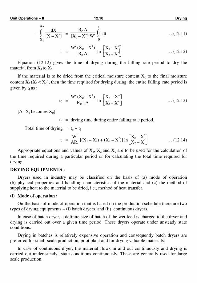
Unit Operations – II 12.10 Drying
– ⌡⌠
X1
X2
dX
[X – X*] =
Rc A
[Xc – X*] W' ⌡⌠
0
t
dt … (12.11)
t = W' (Xc – X*)
Rc A ln
X1 – X*
X2 – X* … (12.12)
Equation (12.12) gives the time of drying during the falling rate period to dry the
material from X1 to X2.
If the material is to be dried from the critical moisture content Xc to the final moisture
content X2 (X2 < Xc), then the time required for drying during the entire falling rate period is
given by tf as :
tf = W' (Xc – X*)
Rc · A ln
Xc – X*
X2 – X* … (12.13)
[As X1 becomes Xc]
tf = drying time during entire falling rate period.
Total time of drying = tc + tf
t = W'
ARc [(X1 – Xc) + (Xc – X
*)] ln
Xc – X
*
X2 – X* … (12.14)
Appropriate equations and values of X1, X2 and Xc are to be used for the calculation of
the time required during a particular period or for calculating the total time required for
drying.
DRYING EQUIPMENTS :
Dryers used in industry may be classified on the basis of (a) mode of operation
(b) physical properties and handling characteristics of the material and (c) the method of
supplying heat to the material to be dried, i.e., method of heat transfer.
(i) Mode of operation :
On the basis of mode of operation that is based on the production schedule there are two
types of drying equipments – (i) batch dryers and (ii) continuous dryers.
In case of batch dryer, a definite size of batch of the wet feed is charged to the dryer and
drying is carried out over a given time period. These dryers operate under unsteady state
conditions.
Drying in batches is relatively expensive operation and consequently batch dryers are
preferred for small-scale production, pilot plant and for drying valuable materials.
In case of continuous dryer, the material flows in and out continuously and drying is
carried out under steady state conditions continuously. These are generally used for large
scale production.
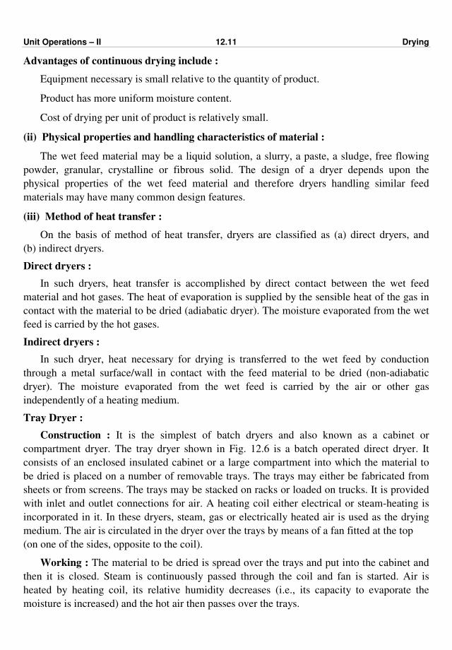
Unit Operations – II 12.11 Drying
Advantages of continuous drying include :
Equipment necessary is small relative to the quantity of product.
Product has more uniform moisture content.
Cost of drying per unit of product is relatively small.
(ii) Physical properties and handling characteristics of material :
The wet feed material may be a liquid solution, a slurry, a paste, a sludge, free flowing
powder, granular, crystalline or fibrous solid. The design of a dryer depends upon the
physical properties of the wet feed material and therefore dryers handling similar feed
materials may have many common design features.
(iii) Method of heat transfer :
On the basis of method of heat transfer, dryers are classified as (a) direct dryers, and
(b) indirect dryers.
Direct dryers :
In such dryers, heat transfer is accomplished by direct contact between the wet feed
material and hot gases. The heat of evaporation is supplied by the sensible heat of the gas in
contact with the material to be dried (adiabatic dryer). The moisture evaporated from the wet
feed is carried by the hot gases.
Indirect dryers :
In such dryer, heat necessary for drying is transferred to the wet feed by conduction
through a metal surface/wall in contact with the feed material to be dried (non-adiabatic
dryer). The moisture evaporated from the wet feed is carried by the air or other gas
independently of a heating medium.
Tray Dryer :
Construction : It is the simplest of batch dryers and also known as a cabinet or
compartment dryer. The tray dryer shown in Fig. 12.6 is a batch operated direct dryer. It
consists of an enclosed insulated cabinet or a large compartment into which the material to
be dried is placed on a number of removable trays. The trays may either be fabricated from
sheets or from screens. The trays may be stacked on racks or loaded on trucks. It is provided
with inlet and outlet connections for air. A heating coil either electrical or steam-heating is
incorporated in it. In these dryers, steam, gas or electrically heated air is used as the drying
medium. The air is circulated in the dryer over the trays by means of a fan fitted at the top
(on one of the sides, opposite to the coil).
Working : The material to be dried is spread over the trays and put into the cabinet and
then it is closed. Steam is continuously passed through the coil and fan is started. Air is
heated by heating coil, its relative humidity decreases (i.e., its capacity to evaporate the
moisture is increased) and the hot air then passes over the trays.
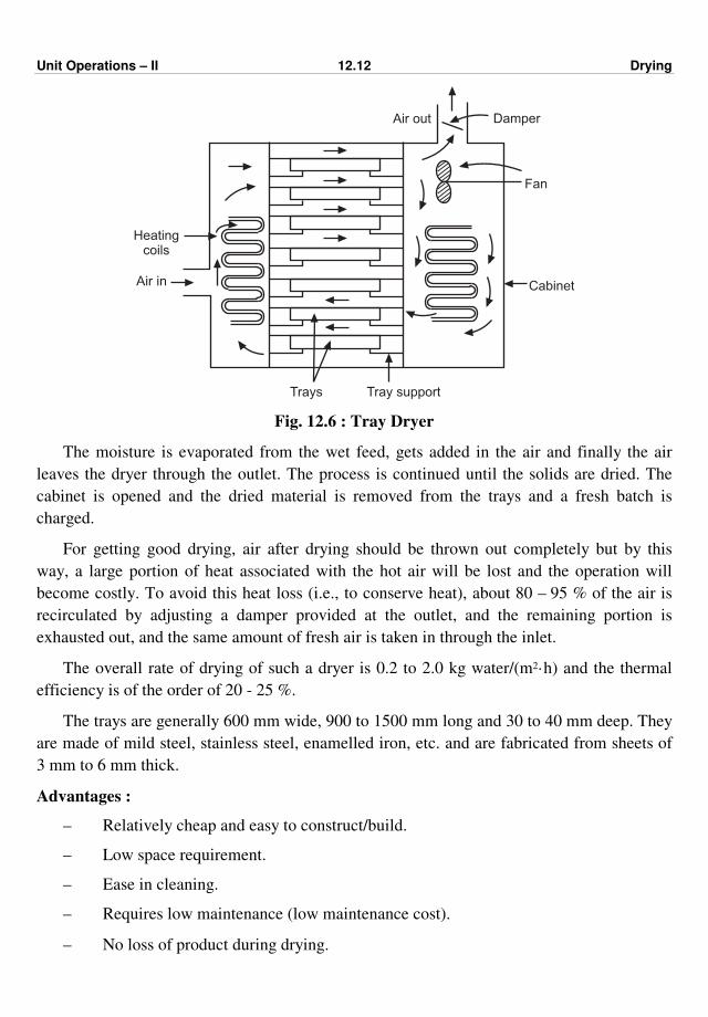
Unit Operations – II 12.12 Drying
Heatingcoils
Air in
Trays Tray support
Cabinet
Fan
DamperAir out
Fig. 12.6 : Tray Dryer
The moisture is evaporated from the wet feed, gets added in the air and finally the air
leaves the dryer through the outlet. The process is continued until the solids are dried. The
cabinet is opened and the dried material is removed from the trays and a fresh batch is
charged.
For getting good drying, air after drying should be thrown out completely but by this
way, a large portion of heat associated with the hot air will be lost and the operation will
become costly. To avoid this heat loss (i.e., to conserve heat), about 80 – 95 % of the air is
recirculated by adjusting a damper provided at the outlet, and the remaining portion is
exhausted out, and the same amount of fresh air is taken in through the inlet.
The overall rate of drying of such a dryer is 0.2 to 2.0 kg water/(m2·h) and the thermal
efficiency is of the order of 20 - 25 %.
The trays are generally 600 mm wide, 900 to 1500 mm long and 30 to 40 mm deep. They
are made of mild steel, stainless steel, enamelled iron, etc. and are fabricated from sheets of
3 mm to 6 mm thick.
Advantages :
– Relatively cheap and easy to construct/build.
– Low space requirement.
– Ease in cleaning.
– Requires low maintenance (low maintenance cost).
– No loss of product during drying.
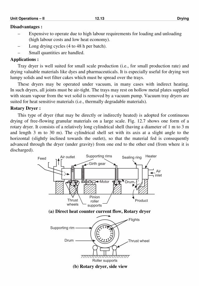
Unit Operations – II 12.13 Drying
Disadvantages :
– Expensive to operate due to high labour requirements for loading and unloading
(high labour costs and low heat economy).
– Long drying cycles (4 to 48 h per batch).
– Small quantities are handled.
Applications :
Tray dryer is well suited for small scale production (i.e., for small production rate) and
drying valuable materials like dyes and pharmaceuticals. It is especially useful for drying wet
lumpy solids and wet filter cakes which must be spread over the trays.
These dryers may be operated under vacuum, in many cases with indirect heating.
In such dryers, all joints must be air-tight. The trays may rest on hollow metal plates supplied
with steam vapour from the wet solid is removed by a vacuum pump. Vacuum tray dryers are
suited for heat sensitive materials (i.e., thermally degradable materials).
Rotary Dryer :
This type of dryer (that may be directly or indirectly heated) is adopted for continuous
drying of free-flowing granular materials on a large scale. Fig. 12.7 shows one form of a
rotary dryer. It consists of a relatively long cylindrical shell (having a diameter of 1 m to 3 m
and length 3 m to 30 m). The cylindrical shell set with its axis at a slight angle to the
horizontal (slightly inclined towards the outlet), so that the material fed is consequently
advanced through the dryer (under gravity) from one end to the other end (from where it is
discharged).
Supporting rimsAir outletFeed
Thrustwheels
Pinionroller
supports
DrumMotor
Product
Airinlet
Sealing ring Heater
Girth gear
(a) Direct heat counter current flow, Rotary dryer
Drum Thrust wheel
Roller supports
Supporting rim
Flights
(b) Rotary dryer, side view
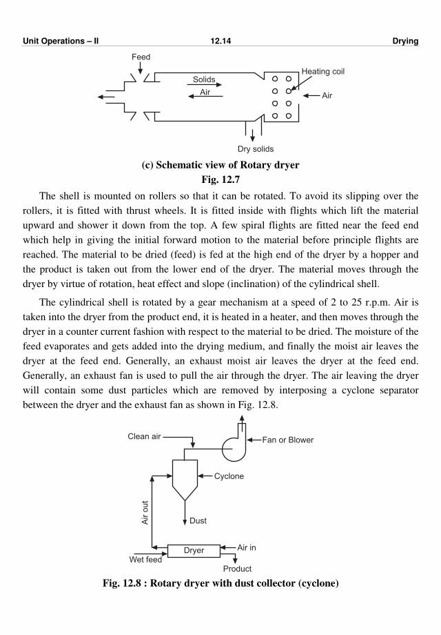
Unit Operations – II 12.14 Drying
Dry solids
Air
Heating coilSolids
Air
Feed
(c) Schematic view of Rotary dryer
Fig. 12.7
The shell is mounted on rollers so that it can be rotated. To avoid its slipping over the
rollers, it is fitted with thrust wheels. It is fitted inside with flights which lift the material
upward and shower it down from the top. A few spiral flights are fitted near the feed end
which help in giving the initial forward motion to the material before principle flights are
reached. The material to be dried (feed) is fed at the high end of the dryer by a hopper and
the product is taken out from the lower end of the dryer. The material moves through the
dryer by virtue of rotation, heat effect and slope (inclination) of the cylindrical shell.
The cylindrical shell is rotated by a gear mechanism at a speed of 2 to 25 r.p.m. Air is
taken into the dryer from the product end, it is heated in a heater, and then moves through the
dryer in a counter current fashion with respect to the material to be dried. The moisture of the
feed evaporates and gets added into the drying medium, and finally the moist air leaves the
dryer at the feed end. Generally, an exhaust moist air leaves the dryer at the feed end.
Generally, an exhaust fan is used to pull the air through the dryer. The air leaving the dryer
will contain some dust particles which are removed by interposing a cyclone separator
between the dryer and the exhaust fan as shown in Fig. 12.8.
Fan or BlowerClean air
Cyclone
Air in
Product
DryerWet feed
Air o
ut
Dust
Fig. 12.8 : Rotary dryer with dust collector (cyclone)
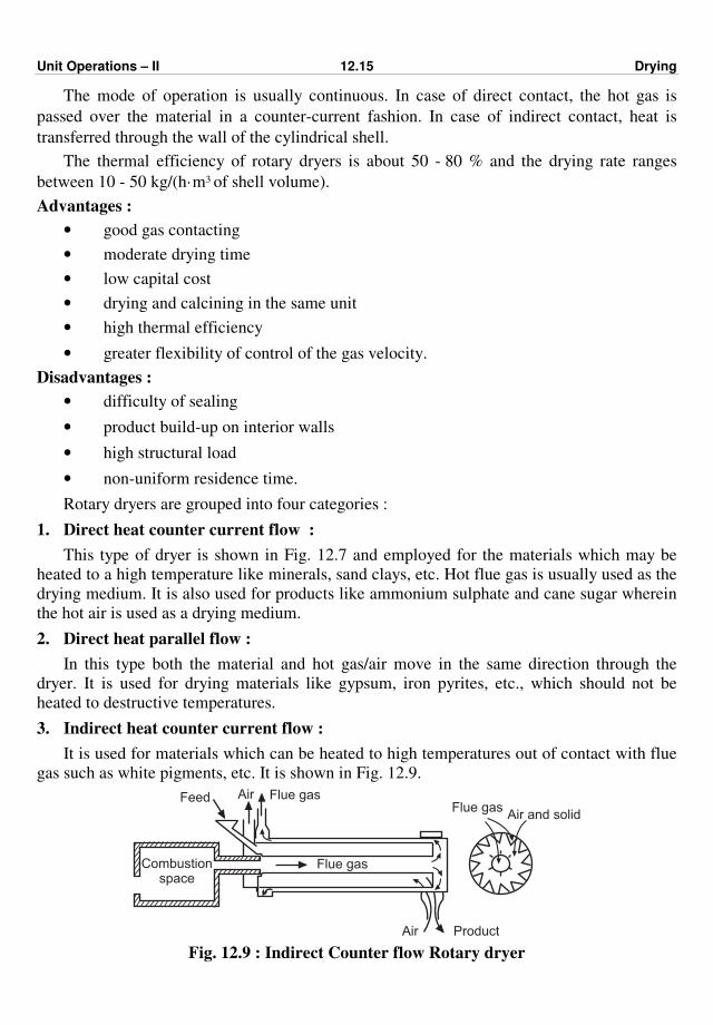
Unit Operations – II 12.15 Drying
The mode of operation is usually continuous. In case of direct contact, the hot gas is
passed over the material in a counter-current fashion. In case of indirect contact, heat is
transferred through the wall of the cylindrical shell.
The thermal efficiency of rotary dryers is about 50 - 80 % and the drying rate ranges
between 10 - 50 kg/(h·m3 of shell volume).
Advantages :
• good gas contacting
• moderate drying time
• low capital cost
• drying and calcining in the same unit
• high thermal efficiency
• greater flexibility of control of the gas velocity.
Disadvantages :
• difficulty of sealing
• product build-up on interior walls
• high structural load
• non-uniform residence time.
Rotary dryers are grouped into four categories :
1. Direct heat counter current flow :
This type of dryer is shown in Fig. 12.7 and employed for the materials which may be
heated to a high temperature like minerals, sand clays, etc. Hot flue gas is usually used as the
drying medium. It is also used for products like ammonium sulphate and cane sugar wherein
the hot air is used as a drying medium.
2. Direct heat parallel flow :
In this type both the material and hot gas/air move in the same direction through the
dryer. It is used for drying materials like gypsum, iron pyrites, etc., which should not be
heated to destructive temperatures.
3. Indirect heat counter current flow :
It is used for materials which can be heated to high temperatures out of contact with flue
gas such as white pigments, etc. It is shown in Fig. 12.9.
Combustionspace
Feed Air Flue gas
Flue gas
Air Product
Flue gasAir and solid
Fig. 12.9 : Indirect Counter flow Rotary dryer
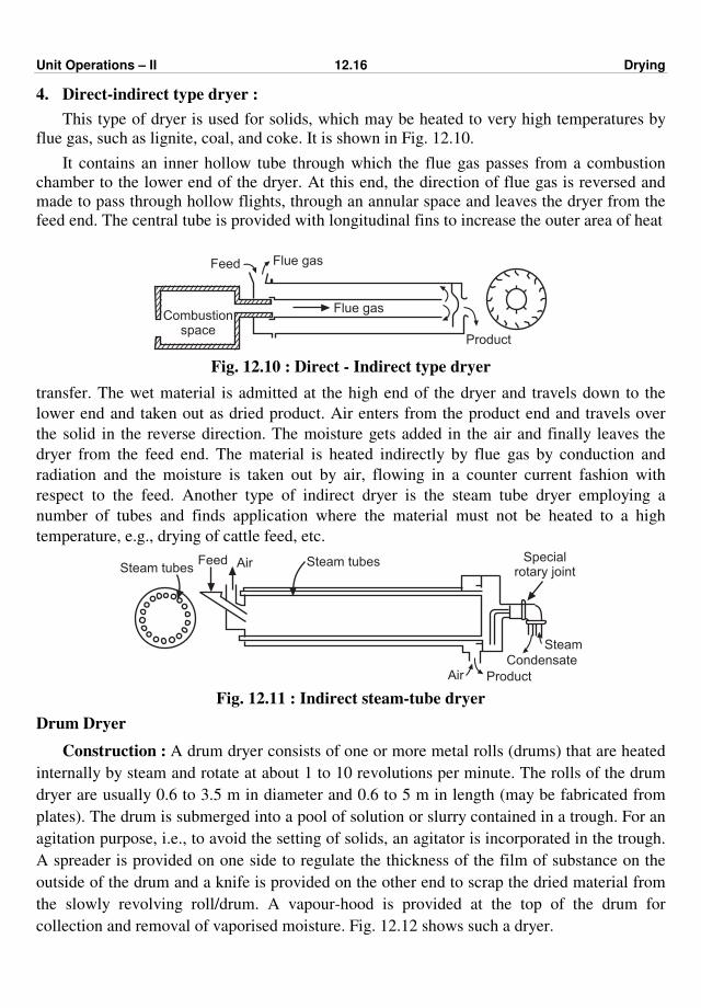
Unit Operations – II 12.16 Drying
4. Direct-indirect type dryer :
This type of dryer is used for solids, which may be heated to very high temperatures by
flue gas, such as lignite, coal, and coke. It is shown in Fig. 12.10.
It contains an inner hollow tube through which the flue gas passes from a combustion
chamber to the lower end of the dryer. At this end, the direction of flue gas is reversed and
made to pass through hollow flights, through an annular space and leaves the dryer from the
feed end. The central tube is provided with longitudinal fins to increase the outer area of heat
Combustionspace
Feed Flue gas
Flue gas
Product
Fig. 12.10 : Direct - Indirect type dryer
transfer. The wet material is admitted at the high end of the dryer and travels down to the
lower end and taken out as dried product. Air enters from the product end and travels over
the solid in the reverse direction. The moisture gets added in the air and finally leaves the
dryer from the feed end. The material is heated indirectly by flue gas by conduction and
radiation and the moisture is taken out by air, flowing in a counter current fashion with
respect to the feed. Another type of indirect dryer is the steam tube dryer employing a
number of tubes and finds application where the material must not be heated to a high
temperature, e.g., drying of cattle feed, etc.
Steam tubes
Steam
Condensate
ProductAir
Specialrotary joint
Steam tubesAirFeed
Fig. 12.11 : Indirect steam-tube dryer
Drum Dryer
Construction : A drum dryer consists of one or more metal rolls (drums) that are heated
internally by steam and rotate at about 1 to 10 revolutions per minute. The rolls of the drum
dryer are usually 0.6 to 3.5 m in diameter and 0.6 to 5 m in length (may be fabricated from
plates). The drum is submerged into a pool of solution or slurry contained in a trough. For an
agitation purpose, i.e., to avoid the setting of solids, an agitator is incorporated in the trough.
A spreader is provided on one side to regulate the thickness of the film of substance on the
outside of the drum and a knife is provided on the other end to scrap the dried material from
the slowly revolving roll/drum. A vapour-hood is provided at the top of the drum for
collection and removal of vaporised moisture. Fig. 12.12 shows such a dryer.
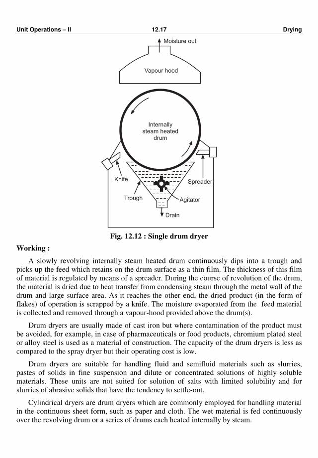
Unit Operations – II 12.17 Drying
Internallysteam heated
drum
Vapour hood
Moisture out
Knife
Trough
Drain
Agitator
Spreader
Fig. 12.12 : Single drum dryer
Working :
A slowly revolving internally steam heated drum continuously dips into a trough and
picks up the feed which retains on the drum surface as a thin film. The thickness of this film
of material is regulated by means of a spreader. During the course of revolution of the drum,
the material is dried due to heat transfer from condensing steam through the metal wall of the
drum and large surface area. As it reaches the other end, the dried product (in the form of
flakes) of operation is scrapped by a knife. The moisture evaporated from the feed material
is collected and removed through a vapour-hood provided above the drum(s).
Drum dryers are usually made of cast iron but where contamination of the product must
be avoided, for example, in case of pharmaceuticals or food products, chromium plated steel
or alloy steel is used as a material of construction. The capacity of the drum dryers is less as
compared to the spray dryer but their operating cost is low.
Drum dryers are suitable for handling fluid and semifluid materials such as slurries,
pastes of solids in fine suspension and dilute or concentrated solutions of highly soluble
materials. These units are not suited for solution of salts with limited solubility and for
slurries of abrasive solids that have the tendency to settle-out.
Cylindrical dryers are drum dryers which are commonly employed for handling material
in the continuous sheet form, such as paper and cloth. The wet material is fed continuously
over the revolving drum or a series of drums each heated internally by steam.
Unit Operations – II 12.18 Drying
Spray Dryer :
It is a continuous direct contact dryer employed for drying of solutions, slurries, and
pastes. In this dryer, a liquid solution or slurry is introduced in the form of very fine droplets
into a stream of hot gas inside a large drying chamber, thereby a large contact area becomes
available for perfect drying. The moisture of feed is evaporated and gets added into the hot
gas.
Construction : Fig. 12.13 shows a typical spray dryer. The essential components of the
dryer are : a drying chamber (a vertical cylindrical chamber with a short conical bottom),
where the feed material is contacted with a hot gas (air), a heater for heating the fresh air
sucked by a fan or blower, cyclone separators for dust separation and collection, a pneumatic
conveying duct and blowers, which are assembled as shown in Fig. 12.13. The material is
usually spread in the form of a mist of fine droplets by spray nozzles or high speed rotating
spray discs into a hot gas stream inside the chamber as shown in Fig. 12.13.
Working : The feed is pumped to the top of the dryer (drying chamber) where it is
disintegrated into small droplets by an atomiser. The large quantity of fresh air is taken in by
a fan, it is heated in a heater and finally fed below the atomiser in the drying chamber. As the
surface area of drops is very large, the liquid portion of these drops rapidly evaporates and
before they touch the bottom of the drying chamber they are completely dried. This
dried product (in the form of dry powder) is taken out and conveyed to a cyclone dust
collector-2 by a stream of air. The major portion of the air is taken out through the air outlet
duct which mostly contains dust and is sent to a cyclone-1. The solids collected by the
cyclone-1 are fed to a pneumatic conveying duct. The air leaving the cyclone - 2 may contain
some dust and therefore it is sent to the cyclone - 1, for further separation, by the fan. The air
from the cyclone -1 is thrown out to the atmosphere by a blower. The dried product from the
cyclone-2 is collected in a dry product collector.
An atomiser is a device which causes the liquid to be disintegrated into the fine drops.
The atomisers commonly used are :
1. Pressure nozzles which make use of pressure energy for atomisation.
2. Two fluid nozzles wherein air or steam at a certain pressure is used to tear a liquid
into droplets, i.e., they make use of gas energy and
3. Rotating discs make use of centrifugal energy for atomisation. Spray nozzles (type -1
and type - 2) are relatively inflexible in operation and also subject to erosion and tear.
The rotating discs (may be plane, vaned or cup-shaped) rotate at a speed of about
3000 to 12000 r.p.m. The feed introduced at the centre of disc is centrifugally
accelerated to the periphery and ultimately thrown in an umbrella-shaped spray. The
rotating discs are very flexible in their operating characteristics and can handle thick
slurries without danger of clogging.

Unit Operations – II 12.19 Drying
Heater
Compressed airPneumatic
conveying duct
Dryproductcollector
Cyclone-2
Fan
Feed Atomiser
Feed
Fan
Air in
Cyclone-1air outlet
duct
Fig. 12.13 : Spray Dryer
In this dryer, care must be taken to ensure that the droplets or wet particles of solids do
not strike and stick to the solid surfaces before complete drying. So as to avoid this, large
drying chambers are used.
Advantages :
• very short drying times (2 – 20 s)
• handle heat sensitive products
• control of a product particle size
• rapid dehydration.
• relatively low operating costs, particularly in large capacity units.
Disadvantages :
• low solids content
• relatively large units
• maintenance of atomiser
• inefficient in (its) energy use
• product built-up on interior walls.
Applications :
These dryers are common in dairy industry, food industry, detergent industry, chemical
and dyes industry.
Spray dryers are widely used for products such as milk powder, detergents, dyes, coffee,
pharmaceuticals, etc.
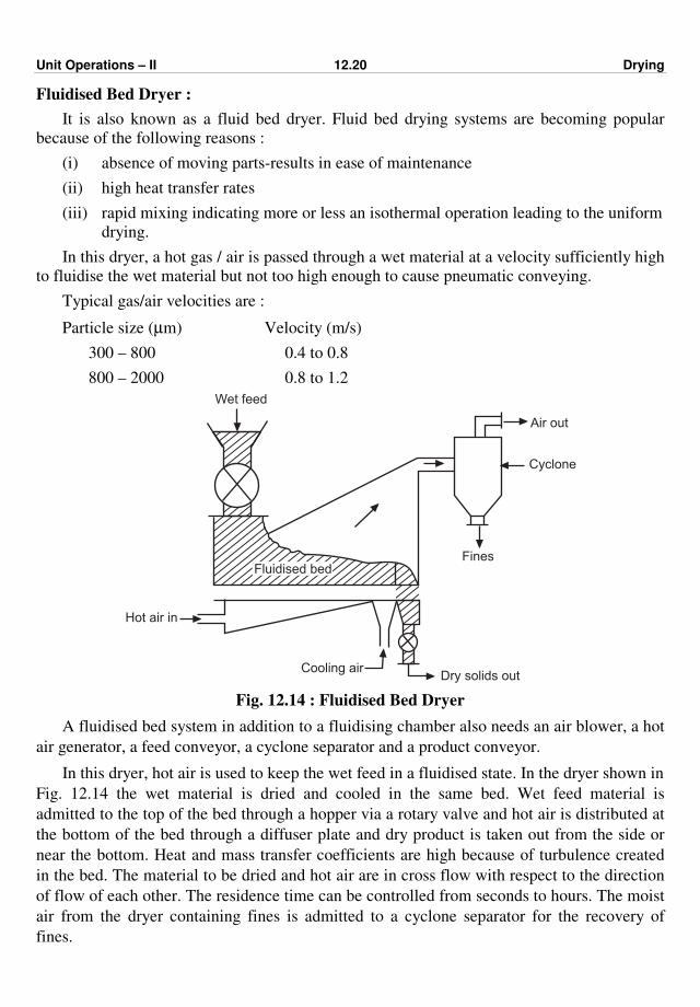
Unit Operations – II 12.20 Drying
Fluidised Bed Dryer :
It is also known as a fluid bed dryer. Fluid bed drying systems are becoming popular
because of the following reasons :
(i) absence of moving parts-results in ease of maintenance
(ii) high heat transfer rates
(iii) rapid mixing indicating more or less an isothermal operation leading to the uniform
drying.
In this dryer, a hot gas / air is passed through a wet material at a velocity sufficiently high
to fluidise the wet material but not too high enough to cause pneumatic conveying.
Typical gas/air velocities are :
Particle size (µm) Velocity (m/s)
300 – 800 0.4 to 0.8
800 – 2000 0.8 to 1.2
Air out
Cyclone
Wet feed
Hot air in
Cooling airDry solids out
FinesFluidised bed
Fig. 12.14 : Fluidised Bed Dryer
A fluidised bed system in addition to a fluidising chamber also needs an air blower, a hot
air generator, a feed conveyor, a cyclone separator and a product conveyor.
In this dryer, hot air is used to keep the wet feed in a fluidised state. In the dryer shown in
Fig. 12.14 the wet material is dried and cooled in the same bed. Wet feed material is
admitted to the top of the bed through a hopper via a rotary valve and hot air is distributed at
the bottom of the bed through a diffuser plate and dry product is taken out from the side or
near the bottom. Heat and mass transfer coefficients are high because of turbulence created
in the bed. The material to be dried and hot air are in cross flow with respect to the direction
of flow of each other. The residence time can be controlled from seconds to hours. The moist
air from the dryer containing fines is admitted to a cyclone separator for the recovery of
fines.
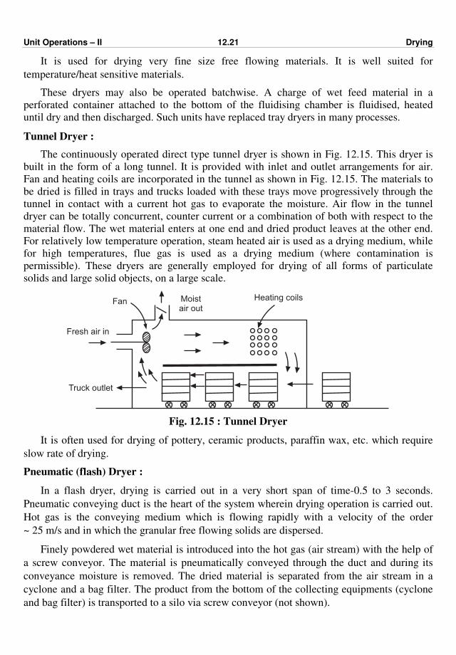
Unit Operations – II 12.21 Drying
It is used for drying very fine size free flowing materials. It is well suited for
temperature/heat sensitive materials.
These dryers may also be operated batchwise. A charge of wet feed material in a
perforated container attached to the bottom of the fluidising chamber is fluidised, heated
until dry and then discharged. Such units have replaced tray dryers in many processes.
Tunnel Dryer :
The continuously operated direct type tunnel dryer is shown in Fig. 12.15. This dryer is
built in the form of a long tunnel. It is provided with inlet and outlet arrangements for air.
Fan and heating coils are incorporated in the tunnel as shown in Fig. 12.15. The materials to
be dried is filled in trays and trucks loaded with these trays move progressively through the
tunnel in contact with a current hot gas to evaporate the moisture. Air flow in the tunnel
dryer can be totally concurrent, counter current or a combination of both with respect to the
material flow. The wet material enters at one end and dried product leaves at the other end.
For relatively low temperature operation, steam heated air is used as a drying medium, while
for high temperatures, flue gas is used as a drying medium (where contamination is
permissible). These dryers are generally employed for drying of all forms of particulate
solids and large solid objects, on a large scale.
Fan Moistair out
Fresh air in
Truck outlet
Heating coils
Fig. 12.15 : Tunnel Dryer
It is often used for drying of pottery, ceramic products, paraffin wax, etc. which require
slow rate of drying.
Pneumatic (flash) Dryer :
In a flash dryer, drying is carried out in a very short span of time-0.5 to 3 seconds.
Pneumatic conveying duct is the heart of the system wherein drying operation is carried out.
Hot gas is the conveying medium which is flowing rapidly with a velocity of the order
~ 25 m/s and in which the granular free flowing solids are dispersed.
Finely powdered wet material is introduced into the hot gas (air stream) with the help of
a screw conveyor. The material is pneumatically conveyed through the duct and during its
conveyance moisture is removed. The dried material is separated from the air stream in a
cyclone and a bag filter. The product from the bottom of the collecting equipments (cyclone
and bag filter) is transported to a silo via screw conveyor (not shown).

Unit Operations – II 12.22 Drying
Air out
6
5
4
Dry solid out
2
1
Air in 3
Wet feed
Fig. 12.16 : Pneumatic (Flash) dryer
1 : drying duct 2 : Heater 3; 6 : blower, 4 : cyclone and 5 : bag filter
Due to very short residence time these dryers are used for drying of heat sensitive
materials.
SOLVED EXAMPLES
Example 12.1 : Wet solids are to be dried from 80 % to 5 % moisture (wet basis).
Calculate the amount of moisture to be evaporated per 100 kg of the dried product.
Solution : Basis : 100 kg dried product obtained.
dry solids in the product = 0.95 × 100 = 95 kg
moisture in the product = 0.05 × 100 = 5 kg
Let x be the kg of wet solids,
moisture in the wet solid = 80 %
Material balance of solids :
solids in wet solid feed = solids in dried product
0.20 x = 95
x = 475 kg
Moisture in the wet solid = 0.80 × 475 = 380 kg
Amount of moisture to be evaporated per 100 kg of the dried product is
= moisture in wet feed – moisture in dried product
= 380 – 5 = 375 kg … Ans.
Example 12.2 : Find out the rate of drying and moisture content from the following
data :
Weight of wet saw dust Weight of saw dust after drying Time (h)
250 g
250 g
230 g
215 g
0.5
0.75
Dimension of tray = 10 cm × 10 cm
Weight of dry saw dust on tray = 150 g
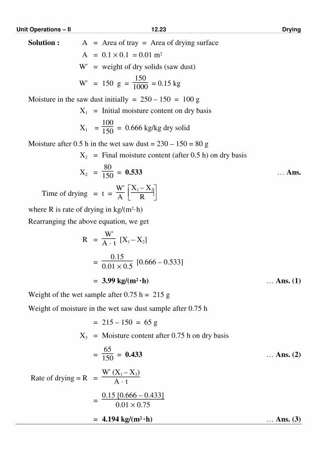
Unit Operations – II 12.23 Drying
Solution : A = Area of tray = Area of drying surface
A = 0.1 × 0.1 = 0.01 m2
W' = weight of dry solids (saw dust)
W' = 150 g = 150
1000 = 0.15 kg
Moisture in the saw dust initially = 250 – 150 = 100 g
X1 = Initial moisture content on dry basis
X1 = 100
150 = 0.666 kg/kg dry solid
Moisture after 0.5 h in the wet saw dust = 230 – 150 = 80 g
X2 = Final moisture content (after 0.5 h) on dry basis
X2 = 80
150 = 0.533 … Ans.
Time of drying = t = W'A
X1 – X2
R
where R is rate of drying in kg/(m2·h)
Rearranging the above equation, we get
R = W'
A · t [X1 – X2]
= 0.15
0.01 × 0.5 [0.666 – 0.533]
= 3.99 kg/(m2 ·h) … Ans. (1)
Weight of the wet sample after 0.75 h = 215 g
Weight of moisture in the wet saw dust sample after 0.75 h
= 215 – 150 = 65 g
X3 = Moisture content after 0.75 h on dry basis
= 65
150 = 0.433 … Ans. (2)
Rate of drying = R = W' (X1 – X3)
A · t
= 0.15 [0.666 – 0.433]
0.01 × 0.75
= 4.194 kg/(m2 ·h) … Ans. (3)

Unit Operations – II 12.24 Drying
Example 12.3 : A batch of wet solids is to be dried from 35 % to 10 % moisture under
constant drying conditions in five hours. If the equilibrium moisture content is 4 % and the
critical moisture content is 14 %. Estimate the time required to dry the solids to 6 %
moisture under the same drying conditions. All moisture content are on the wet basis.
Solution : Case-I :
Initial moisture = 35 %
Final moisture = 10 %
Critical moisture = 14 %
and Equilibrium moisture = 4 %
Time required for drying the solids from 35 % to 10 % moisture = 5 h
It is clear from the values of the moisture content given above (final moisture and critical
moisture) that the period of five hours will be the time required during the constant rate
period plus the time required during the falling rate period.
Let x = wt. fraction of moisture in the solids = (wt. %)/100
X1 = Initial moisture content on dry basis
= x1
1 – x1 =
0.35
1 – 0.35 = 0.5385
Xc = Critical moisture content on dry basis
= xc
1 – xc =
0.14
1 – 0.14 = 0.1628
X* = Equilibrium moisture content
= x*
1 – x* = 0.04
1 – 0.04 = 0.0417
X2 = Final moisture content (in the falling rate period)
= x2
1 – x2 =
0.1
1 – 0.1 = 0.111
t = Time of drying
= tc + tf
The time required for drying is given by
t = W'
A · Rc [X1 – Xc] +
W' (Xc – X*)
Rc · A ln
Xc – X*
X2 – X*
where Rc = rate of drying in constant rate period
W' = kg of dry solids
A = area of drying surface.
The above equation can be written as
t = W'
A · Rc
(X1 – Xc) + (Xc – X*) ln
Xc – X*
X2 – X* … (1)

Unit Operations – II 12.25 Drying
Substituting the values of t, X1, X2, Xc and X*, we get
5 = W'
Rc · A
(0.5385 – 0.1628) + (0.1628 – 0.0417) ln
0.1628 – 0.0417
0.111 – 0.0417
∴ W'
Rc · A = 11.28
Case-II : The final moisture in this case is given as 6 %
∴ X2 = Final moisture content on dry basis
= 0.06
1 – 0.06 = 0.0638
Using Equation (1) and substituting the values of the various terms involved, the time for
drying the solids from 35 % to 6 % moisture is
t = W'
Rc · A
(X1 – Xc) + (Xc – X*) ln
Xc – X*
X2 – X*
t = (11.28)
(0.5385 – 0.1628) + (0.1628 – 0.0417) ln
0.1628 – 0.0417
0.0638 – 0.0417
t = 6.56 h … Ans.
Example 12.4 : A 100 kg bath of granular solids containing 30 % moisture is to be dried
in a tray dryer to 16 % moisture by passing a current of air at 350 K tangentially across its
surface at a velocity of 1.8 m/s. If the constant rate of drying under these conditions is
0.7 × 10⁻³ kg/(m2·s) and the critical moisture content is 15 %, calculate the time required for
drying the solids.
Drying surface = 0.03 m2/kg dry weight.
Solution : Moisture content data for the constant rate period is
Initial moisture = 30 % … on wet basis
Final moisture = 16 %
Critical moisture = 15 %
As the final moisture is greater than the critical moisture, we are in the constant rate
period. The equation for calculating the time of drying during the constant rate period is
t = W'A
X1 – X2
Rc
where W' = weight of dry solids
A = Area of drying surface (surface area available for drying)
and X1 and X2 are the initial and final moisture contents (dry basis), respectively.
X1 = Initial moisture content (dry basis)
= 0.3
1 – 0.3 = 0.428
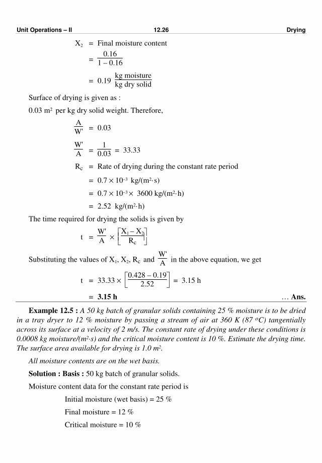
Unit Operations – II 12.26 Drying
X2 = Final moisture content
= 0.16
1 – 0.16
= 0.19 kg moisture
kg dry solid
Surface of drying is given as :
0.03 m2 per kg dry solid weight. Therefore,
A
W' = 0.03
W'A
= 1
0.03 = 33.33
Rc = Rate of drying during the constant rate period
= 0.7 × 10⁻³ kg/(m2·s)
= 0.7 × 10–3 × 3600 kg/(m2·h)
= 2.52 kg/(m2·h)
The time required for drying the solids is given by
t = W'A
×
X1 – X2
Rc
Substituting the values of X1, X2, Rc and W'
A in the above equation, we get
t = 33.33 ×
0.428 – 0.19
2.52 = 3.15 h
= 3.15 h … Ans.
Example 12.5 : A 50 kg batch of granular solids containing 25 % moisture is to be dried
in a tray dryer to 12 % moisture by passing a stream of air at 360 K (87 oC) tangentially
across its surface at a velocity of 2 m/s. The constant rate of drying under these conditions is
0.0008 kg moisture/(m2·s) and the critical moisture content is 10 %. Estimate the drying time.
The surface area available for drying is 1.0 m2.
All moisture contents are on the wet basis.
Solution : Basis : 50 kg batch of granular solids.
Moisture content data for the constant rate period is
Initial moisture (wet basis) = 25 %
Final moisture = 12 %
Critical moisture = 10 %
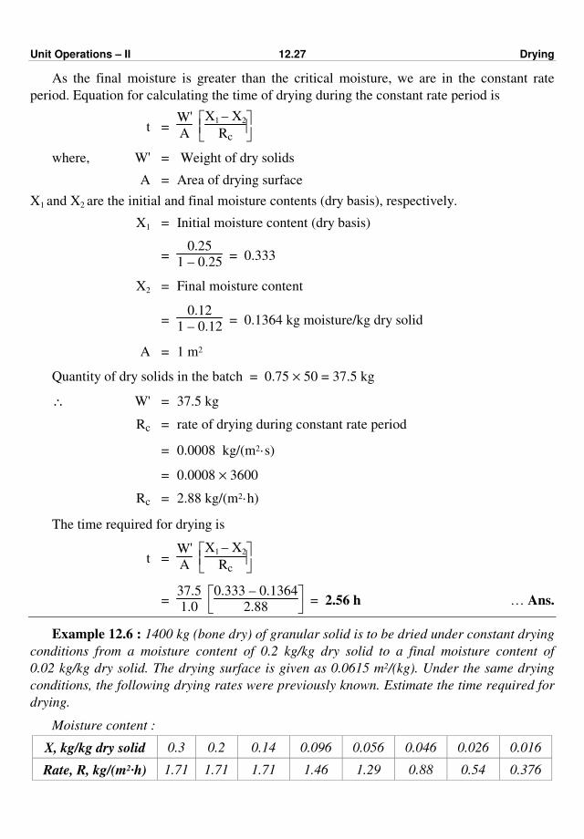
Unit Operations – II 12.27 Drying
As the final moisture is greater than the critical moisture, we are in the constant rate
period. Equation for calculating the time of drying during the constant rate period is
t = W'A
X1 – X2
Rc
where, W' = Weight of dry solids
A = Area of drying surface
X1 and X2 are the initial and final moisture contents (dry basis), respectively.
X1 = Initial moisture content (dry basis)
= 0.25
1 – 0.25 = 0.333
X2 = Final moisture content
= 0.12
1 – 0.12 = 0.1364 kg moisture/kg dry solid
A = 1 m2
Quantity of dry solids in the batch = 0.75 × 50 = 37.5 kg
∴ W' = 37.5 kg
Rc = rate of drying during constant rate period
= 0.0008 kg/(m2·s)
= 0.0008 × 3600
Rc = 2.88 kg/(m2·h)
The time required for drying is
t = W'A
X1 – X2
Rc
= 37.5
1.0
0.333 – 0.1364
2.88 = 2.56 h … Ans.
Example 12.6 : 1400 kg (bone dry) of granular solid is to be dried under constant drying
conditions from a moisture content of 0.2 kg/kg dry solid to a final moisture content of
0.02 kg/kg dry solid. The drying surface is given as 0.0615 m2/(kg). Under the same drying
conditions, the following drying rates were previously known. Estimate the time required for
drying.
Moisture content :
X, kg/kg dry solid 0.3 0.2 0.14 0.096 0.056 0.046 0.026 0.016
Rate, R, kg/(m2·h) 1.71 1.71 1.71 1.46 1.29 0.88 0.54 0.376
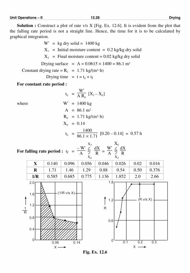
Unit Operations – II 12.28 Drying
Solution : Construct a plot of rate v/s X [Fig. Ex. 12.6]. It is evident from the plot that
the falling rate period is not a straight line. Hence, the time for it is to be calculated by
graphical integration.
W' = kg dry solid = 1400 kg
X1 = Initial moisture content = 0.2 kg/kg dry solid
X2 = Final moisture content = 0.02 kg/kg dry solid
Drying surface = A = 0.0615 × 1400 = 86.1 m2
Constant drying rate = Rc = 1.71 kg/(m2·h)
Drying time = t = tc + tf
For constant rate period :
tc = W'
A Rc [X1 – Xc]
where W' = 1400 kg
A = 86.1 m2
Rc = 1.71 kg/(m2·h)
Xc = 0.14
tc = 1400
86.1 × 1.71 [0.20 – 0.14] = 0.57 h
For falling rate period : tf = – W'
A ⌡⌠
Xc
X2
dX
R =
W'A
⌡⌠
X2
Xc
dX
R
X 0.140 0.096 0.056 0.046 0.026 0.02 0.016
R 1.71 1.46 1.29 0.88 0.54 0.50 0.376
1/R 0.585 0.685 0.775 1.136 1.852 2.0 2.66
1R
1.2
1.6
0.8
0.4
2.0
0
(1/R v/s X)
R
(R v/s X)
1.8
1.2
0.6
0 0.1 0.2 0.3
X
0.140.06
X Fig. Ex. 12.6
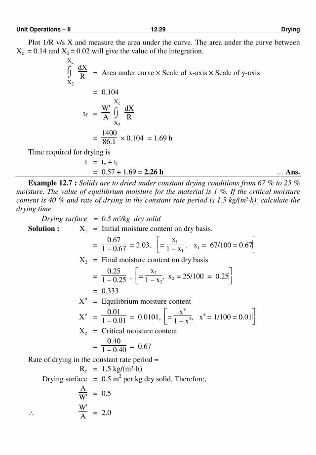
Unit Operations – II 12.29 Drying
Plot 1/R v/s X and measure the area under the curve. The area under the curve between
Xc = 0.14 and X2 = 0.02 will give the value of the integration.
⌡⌠
X2
Xc
dX
R = Area under curve × Scale of x-axis × Scale of y-axis
= 0.104
tf = W'A
⌡⌠
X2
Xc
dX
R
= 1400
86.1 × 0.104 = 1.69 h
Time required for drying is
t = tc + tf
= 0.57 + 1.69 = 2.26 h … Ans.
Example 12.7 : Solids are to dried under constant drying conditions from 67 % to 25 %
moisture. The value of equilibrium moisture for the material is 1 %. If the critical moisture
content is 40 % and rate of drying in the constant rate period is 1.5 kg/(m2·h), calculate the
drying time
Drying surface = 0.5 m2/kg dry solid
Solution : X1 = Initial moisture content on dry basis.
= 0.67
1 – 0.67 = 2.03,
= x1
1 – x1 ‚ x1 = 67/100 = 0.67
X2 = Final moisture content on dry basis
= 0.25
1 – 0.25 ,
= x2
1 – x2, x2 = 25/100 = 0.25
= 0.333
X* = Equilibrium moisture content
X* = 0.01
1 – 0.01 = 0.0101,
= x*
1 – x*, x* = 1/100 = 0.01
Xc = Critical moisture content
= 0.40
1 – 0.40 = 0.67
Rate of drying in the constant rate period =
Rc = 1.5 kg/(m2·h)
Drying surface = 0.5 m2 per kg dry solid. Therefore,
A
W' = 0.5
∴ W'A
= 2.0
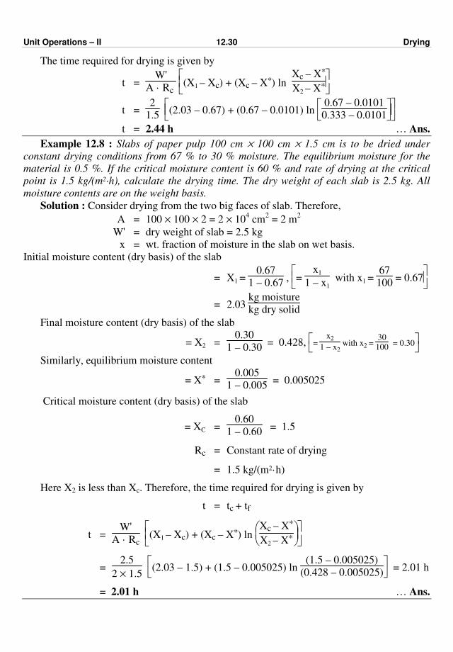
Unit Operations – II 12.30 Drying
The time required for drying is given by
t = W'
A · Rc
(X1 – Xc) + (Xc – X*) ln Xc – X*
X2 – X*
t = 2
1.5
(2.03 – 0.67) + (0.67 – 0.0101) ln
0.67 – 0.0101
0.333 – 0.0101
t = 2.44 h … Ans.
Example 12.8 : Slabs of paper pulp 100 cm × 100 cm × 1.5 cm is to be dried under
constant drying conditions from 67 % to 30 % moisture. The equilibrium moisture for the
material is 0.5 %. If the critical moisture content is 60 % and rate of drying at the critical
point is 1.5 kg/(m2·h), calculate the drying time. The dry weight of each slab is 2.5 kg. All
moisture contents are on the weight basis.
Solution : Consider drying from the two big faces of slab. Therefore,
A = 100 × 100 × 2 = 2 × 104 cm
2 = 2 m
2
W' = dry weight of slab = 2.5 kg
x = wt. fraction of moisture in the slab on wet basis.
Initial moisture content (dry basis) of the slab
= X1 = 0.67
1 – 0.67 ,
= x1
1 – x1 with x1 =
67
100 = 0.67
= 2.03 kg moisture
kg dry solid
Final moisture content (dry basis) of the slab
= X2 = 0.30
1 – 0.30 = 0.428,
=
x2
1 – x2 with x2 =
30
100 = 0.30
Similarly, equilibrium moisture content
= X* = 0.005
1 – 0.005 = 0.005025
Critical moisture content (dry basis) of the slab
= XC = 0.60
1 – 0.60 = 1.5
Rc = Constant rate of drying
= 1.5 kg/(m2·h)
Here X2 is less than Xc. Therefore, the time required for drying is given by
t = tc + tf
t = W'
A · Rc
(X1 – Xc) + (Xc – X*) ln
Xc – X*
X2 – X*
= 2.5
2 × 1.5
(2.03 – 1.5) + (1.5 – 0.005025) ln (1.5 – 0.005025)
(0.428 – 0.005025) = 2.01 h
= 2.01 h … Ans.
Unit Operations – II 12.31 Drying
EXERCISE
1. Fill in the blanks :
(a) ............ refers to the removal of moisture of a substance by thermal means.
Ans. Drying
(b) Removal of moisture by .......... means is more costly than mechanical means.
Ans. thermal
(c) The moisture content in excess of an equilibrium moisture content is called as ....
moisture content. Ans. free
(d) At ......... moisture content, the constant rate period ends and the falling rate period
starts. Ans. critical
(e) Rotating discs make use of ......... energy for atomisation. Ans. centrifugal
(f) For producing milk powder, ........... dryer is used. Ans. spray
(g) ........... dryer is commonly used for wet filter cakes and wet lumpy solids.
Ans. Tray
(h) Drying operation involves the transfer of solute material from the ........ phase to the
gas phase. Ans. solid
2. Define the following terms :
(i) critical moisture content, (ii) equilibrium moisture content, (iii) bound moisture
content and (iv) drying.
3. State the reasons for carrying drying operation industrially.
4. What do you mean by constant drying conditions ?
5. Draw a neat sketch of rate of drying curve and mention various zones on it.
6. Explain in brief rate of drying curve.
7. Draw plots of (i) relative humidity v/s moisture content and moisture content v/s
time.
8. What do you mean by constant rate period and falling rate period ?
9. State the factors on which the rate of drying depends. Explain in brief.
10. Draw a neat sketch of tray dryer and explain its construction.
Unit Operations – II 12.32 Drying
11. Give the advantages, disadvantages and applications of
(i) Tray dryer (ii) Spray dryer.
12. Exlain in brief rotary dryer with respect to its construction and working.
13. Draw a neat sketch of spray dryer and explain its working.
14. How dryers are classified ?
15. Explain in brief fluidised bed dryer.
16. Explain in brief pneumatic (flash) dryer with its sketch.
ppp

(A.1)
APPENDICES
APPENDIX-I
TRY YOURSELF
1. The materials A and B have thermal conductivities as k1 and k2, respectively where
k1 is greater than k2, state which of these materials has a higher resistance to heat
transfer for a given thickness ?
2. Give the unit of thermal conductivity in the SI system.
3. Is thermal conductivity a function of temperature ?
4. Heat flow is inversely proportional to temperature difference. State whether this
statement is correct or not and if not, correct it.
5. Is there temperature variation with time at steady state in a brick walled furnace at
any location ?
6. The pipe has inside diameter of D1 and outside diameter of D2. Express its log mean
radius in terms of D1 and D2 ?
7. In forced convection, heat transfer coefficients are higher than those in natural
convection. State whether this statement is true or false.
8. Name the three resistances in series in case of heat transfer from a hot fluid to a cold
fluid separated by the metal wall.
9. What will happen to the value of heat transfer coefficient, if the velocity of flowing
fluid is increased from u1 to u2 (u2 > u1).
10. Coolants with specific heats of CPA and CP
B are available where CP
A > CP
B . For a
given duty and for the same terminal temperatures of coolants, state which fluid
needs higher mass flow rate through a exchanger.
11. If heat exchanger is put into service for a long time, which is designed without
taking into account fouling what will be the effect on temperatures of the hot and
cold fluids ?
12. If heat exchanger is put into service for long time which is designed based on the
clean overall coefficient, will it transfer the required amount of heat and if not.
Justify your answer.
13. In heat exchange process if one of the fluids is viscous, state whether it should be
directed, on the shell side or tube side of a heat exchanger.
14. In heat exchange process if one of the fluids is corrosive, state whether it should be
directed on the shell side or the tube side of shell and tube heat exchanger.
15. For which heat duty condensers and cooler are used ?
16. What for baffles are incorporated in a shell and tube heat exchanger ?
17. Why the heat transfer coefficients are low in case of film wise condensation ?
18. Which type of surface leads to condensation to proceed in a dropwise manner ?

Unit Operations – II A.2 Appendices
19. State which of the following exchanger has more ability to recover heat:
(1) Parallel flow exchanger.
(2) Counter current flow apparatus.
20. Is it possible in parallel flow for the hot fluid temperature to fall below the outlet
temperature of the cold fluid. If not, state the type of flow in which it is possible.
21. In parallel flow, theoretically, the lowest temperature attainable by the hot fluid is
that of outlet temperature of the cold fluid. If this were obtained what do you think
of heat transfer surface requirement and its feasibility ?
22. What do you understand by nucleate boiling and film boiling ?
23. Why film boiling is not desired in commercial equipments ?
24. Mention whether film heat transfer coefficient is higher in nucleate boiling or in film
boiling ?
25. Which type of pitch arrangement will offer a larger heat transfer surface in a given
shell diameter ?
26. If frequent cleaning is required, which type of pitch arrangement should be adopted
for laying tubes in the tubesheet ?
27. Which type of flow arrangement do you suggest to limit the maximum temperature
of cooler fluid ?
28. Why pipes carrying steam are insulated ?
29. State whether cleaning of the tubes from inside or from outside is easy ?
30. State with which of the following exchanger, the heat recovery will be maximum ?
(1) 1-1 shell and tube exchanger,
(2) 1-2 shell and tube exchanger,
(3) 2-4 shell and tube exchanger.
31. What do you mean by the term "fins" ?
32. In heating of gases or oil say by condensing steam, finned tube units are employed.
Why ?
33. In finned tube units, state whether the fluid having very low heat transfer coefficient
as compared to the other should be directed on the fin side or the other side.
34. Is it possible to take out a tube bundle outside of the shell and clean it in case of
(i) fixed tube sheet exchanger
(ii) U-tube exchanger
(iii) floating head heat exchanger.
35. The problem of differential expansion is eliminated in floating head heat
exchangers. State whether this statement is correct or not ?
36. Does the presence of non condensable gas in the condensing vapour decrease the
film heat transfer coefficient ?
37. State two methods of increasing the steam economy of evaporation system.

Unit Operations – II A.3 Appendices
38. If the condensate formed does not wet the surface, which type condensation do you
expect to occur ?
39. Unlike conduction and convection, energy transfer by radiation does not need
physical contact. State whether this statement is true or false.
40. At high temperature levels, heat loss by radiation from a unlagged steam pipe is very
high as compared heat loss by conduction and convection. State whether this
statement is true or false.
41. Driving force for heat transfer is a temperature difference or gradient. What is the
driving force in case of mass transfer ?
42. Boiling point of the solution is 380 K (107o C) at atmospheric pressure in the vapour
space. What is the boiling point elevation of the solution ?
43. State the operation in which equimolal counter diffusion takes place.
44. Mention the law for mass transfer like Fourier's law for heat transfer.
45. What happens to the product purity if boil-up rate is suddenly increased ?
46. Why actual stages are more than theoretical stages ?
47. State whether a packed column is a continuous contactor or stage wise contactor.
48. Mention the condition which limits the mass transfer.
49. What is the effect of increasing the total pressure on separation by distillation ?
50. State whether the bubble point and dew point are identical for a pure component or
not.
51. State the phases involved in case of
(i) distillation, (ii) crystallization and (iii) drying.
52. State direction of solute transfer in gas absorption.
53. Which factor is a measure of separation by distillation ?
54. What will happen to the boiling point temperature if pressure starts building in
simple distillation still ?
55. What will happen if vaporisation rate is increased above that for which a condenser
is designed in case of distillation. The vent is provided on the condenser.
56. What is the upper limit for bubble point of a binary mixture at a given pressure ?
57. State whether plate or packed column is usually preferred for batch distillation
operation.
58. What is the upper limit for packing size in case of a packed column.
59. In dealing with liquid mixtures containing solids, whether we should go for
continuous process or batch process of distillation to keep the solids separated.
60. Whether cleaning is easy with plate or packing ?
61. What is the common driving force for nucleation and growth of crystals ?
62. Whether cooling should be fast or slow for obtaining large size crystals ?

Unit Operations – II A.4 Appendices
63. Suggest suitable dryer for
(i) milk powder
(ii) wet lumpy solids
(iii) free flowing materials.
64. State whether fluidised bed dryers can be used for heat sensitive materials or not.
65. The solvent used for gas absorption should be non-volatile. Why ?
66. To conserve the heat energy, a major portion of hot air is recirculated in the tray
dryer. State whether this statement is true or false ?
67. What for flights are incorporated in a rotary dryer ?
68. State unit-operations involving simultaneous heat and mass transfer.
69. Why the orifices should be cleaned from time to time in case of spray dryers using
pressure nozzles ?
70. What happens if dryers are not insulated ?
71. Suppose in drying operation, wet bulb temperature of the outgoing air increases.
State what it indicates and state whether the outgoing flow should be increased or
not ?
72. Like relative volatility in distillation, state the factor which is a measure of
separation by liquid-liquid extraction.
73. What do you mean by an azeotrope.
74. Extraction followed by distillation can be thought more economical than distillation
alone in case of a dilute solution of acetic acid. State whether this statement is true
or false ?
75. State the method of achieving supersaturation in case of solutes of which solubility
increases with increase in temperature.
76. Why dispersed phase distributor should be embedded in packings in case of
extraction in a packed column ?
77. State the nature of solutions for which forced circulation evaporators are commonly
employed.
78. In spray tower used for extraction, true counter current is not observed. State
whether it is true or false.
79. In Swenson-Walker crystalliser, what is the role of a spiral agitator ?
80. In steam distillation, if the pressure is atmospheric a boiling temperature is always
less than 373 K (100o C). State whether it is true or false.
ANSWERS (TRY YOURSELF)
1. Material B of thermal conductivity k2.
2. W/(m·K).
3. Yes.
4. No. Heat flow is directly proportional to the temperature difference.
5. No.
Unit Operations – II A.5 Appendices
6. 1
2
(D2 – D1)
ln
D2
D1
7. True.
8. Resistance of the hot fluid film, resistance of the metal wall, and resistance of the
cold fluid film.
9. Film heat transfer coefficients will increase form h1 to h2 (h2 > h1, h2 corresponds
to u2).
10. Coolant having specific heat of CPB
.
11. Temperature of the hot fluid increases and that of the cold fluid falls.
12. No. After a long time in service, scale or dirt deposits on the heat transfer surface
which will add to thermal resistance, the value of U will be reduced and required
amount of heat will be no longer transferred.
13. Viscous fluid should be directed on the shell side.
14. Corrosive fluid should be directed through the tubes.
15. Condensers are employed to remove latent heat and coolers are employed to remove
sensible heat.
16. Baffles reduce the flow area and direct the fluid across the tube bundle which leads
to generation of turbulence in the shell side fluid, thus increasing shell side heat
transfer coefficient.
17. Due to the resistance of condensate film to the heat passing through it, film heat
transfer coefficients are low.
18. Oily and greasy surface, surface on which dirt is present.
19. Counter current flow heat exchanger.
20. No. Counter current flow.
21. LMTD would be zero and as Q and U are finite, surface required would be infinite,
and it is not feasible practically.
22. When vaporisation takes place directly from the surface, it is called nucleate boiling
and when vaporisation takes place through blanketing a film of gas, it is called as
film boiling.
23. Heat transfer rate is much low for large temperature drop and temperature drop is
not utilised effectively.
24. Film heat transfer coefficient is higher in nucleate boiling.
25. Triangular pitch arrangement.
26. Square pitch arrangement.
27. Parallel flow arrangement
28. To avoid heat loss by radiation, convection and conduction i.e. to conserve heat.
29. Cleaning of the tubes from inside is easy.
Unit Operations – II A.6 Appendices
30. 2 – 4 shell and tube exchanger.
31. The metal pieces attached to ordinary tube or pipe to extend (or increase) the heat
transfer surface are called fins.
32. In heating of gas or oil by condensing steam, gas or oil heat transfer coefficient is
very small. Compared that of steam and heat transfer will be controlled by it. So as
to make h × A on the gas side approximately equal to h × A on condensing steam
side, gas or oil surface should be extended with fins. In finned tube units, gas or oil
side surface is extended by fins, hence finned tube units are used for heating of gas
or oil by condensing steam.
33. Fluid having very low film transfer coefficient should be directed on the fin side.
34. (i) No. (ii) Yes. (iii) Yes.
35. This statement is correct.
36. Yes.
37. (i) Multiple effect evaporation (ii) Vapour recompression.
38. Dropwise condensation.
39. This statement is True.
40. This statement is True.
41. Concentration difference.
42. 380 – 373 = 10 K = boiling point elevation of the solution.
43. Distillation.
44. Fick's law.
45. Product purity goes down.
46. While calculating the ideal stages according to the definition of ideal stage, it is
assumed that equilibrium exists between the vapour and liquid leaving the each
stage which is not generally achieved in actual practice, so actual stages are more
than ideal stages.
47. Packed column is a continuous contactor.
48. Equilibrium condition.
49. As the total pressure is increased, the relative volatility decreases and separation
becomes difficult.
50. Bubble point and dew point are identical for a pure component, and are equal to the
boiling point of the pure component at the given pressure.
51. (1) Vapour - liquid (2) Solid - liquid (3) Solid - gas.
52. From gas phase to liquid solvent phase.
53. Relative volatility.
54. Boiling point increases.
55. Vapour loss through vent provided on the condenser.
Unit Operations – II A.7 Appendices
56. Boiling point of a less volatile component at a given system pressure.
57. Packed column (due to low liquid hold-up).
58. Packing size should not be greater than one - eighth of the column diameter.
59. Batch distillation process.
60. Cleaning is easy with plate column.
61. Supersaturation.
62. Cooling should be slow.
63. (i) Spray dryer. (ii) Tray dryer. (iii) Rotary dryer.
64. Yes.
65. The gas leaving the absorption tower is usually saturated with solvent, so to
minimise the loss of solvent with the gas, the solvent should be non- volatile (i.e.
solvent should have low vapour pressure).
66. True.
67. Flights lift the material and shower it down through the current of hot air, otherwise
material to be dried may only slip or roll over the dryer shell.
68. (i) Crystallization (ii) Drying.
69. To avoid clogging.
70. Dryers are insulated to conserve heat and if not insulated, dew may form from inside
of dryer and it may fall on the dried product.
71. Increase in the humidity of outgoing air. The air flow should be increased.
72. Selectivity.
73. An azeotrope is a constant boiling mixture.
74. True.
75. Supersaturation by cooling.
76. If the material of the packing support does not get wet by the dispersed phase
droplets and if the distributor is placed outside the packing, the drop will face
difficulty in entering packing and premature flooding results. For this reason the
distributor is embedded the packing.
77. For viscous, scale forming and salting solutions.
78. True.
80. A spiral agitator prevents the deposition of crystals on a cooling surface, keeps
crystals in suspension (by lifting and showering) to yield crystals of uniformed size
and conveys them from one end to the other end of the crystallizer.
80. True.
ppp
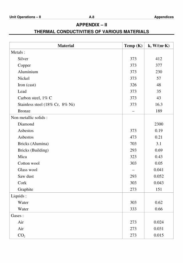
Unit Operations – II A.8 Appendices
APPENDIX – II
THERMAL CONDUCTIVITIES OF VARIOUS MATERIALS
Material Temp (K) k, W/(m·K)
Metals :
Silver
Copper
Aluminium
Nickel
Iron (cast)
Lead
Carbon steel, 1% C
Stainless steel (18% Cr, 8% Ni)
Bronze
373
373
373
373
326
373
373
373
–
412
377
230
57
48
35
43
16.3
189
Non metallic solids :
Diamond
Asbestos
Asbestos
Bricks (Alumina)
Bricks (Building)
Mica
Cotton wool
Glass wool
Saw dust
Cork
Graphite
373
473
703
293
323
303
–
293
303
273
2300
0.19
0.21
3.1
0.69
0.43
0.05
0.041
0.052
0.043
151
Liquids :
Water
Water
303
333
0.62
0.66
Gases :
Air
Air
CO2
273
273
273
0.024
0.031
0.015

Unit Operations – II A.9 Appendices
APPENDIX – III
STEAM TABLES
NOTATION USED
p = Absolute pressure in mm Hg, kPa or MPa
t = Saturation temperture in oC
T = Sautration temperature in K
h = Specific enthalpy of saturated or compressed water in kJ/kg
H = Specific enthalpy of saturated steam in kJ/kg
λ = Latent heat of vaporization of saturated water in kJ/kg
Table 1 : Properteis of saturated water and saturated steam up to atmospheric pressure
p
mm Hg
p
kPa
t oC
T
K
h
kJ/kg
H
kJ/kg
λλλλ
kJ/kg
1
2
3
0.133
0.267
0.400
– 19.302
– 10.902
– 5.693
253.848
262.248
267.457
– 82.56
– 46.30
– 24.12
2466.0
2481.5
2491.1
2548.6
2527.8
2515.2
4
5
6
7
8
9
10
11
12
13
14
15
16
17
18
19
20
21
22
0.533
0.667
0.800
0.933
1.067
1.200
1.333
1.467
1.600
1.733
1.867
2.000
2.133
2.266
2.400
2.533
2.666
2.800
2.933
– 1.854
1.210
3.772
5.980
7.926
9.667
11.246
12.691
14.025
15.265
16.423
17.511
18.538
19.509
20.432
21.311
22.150
22.954
23.724
271.296
274.360
276.922
279.130
281.076
282.817
284.396
285.841
287.175
288.415
289.573
290.661
291.688
292.659
293.582
294.461
295.300
296.104
296.874
– 7.87
5.06
15.84
25.13
33.29
40.60
47.22
53.27
58.86
64.05
68.90
73.45
77.74
81.81
85.67
89.34
92.85
96.21
99.43
2498.1
2503.8
2508.5
2512.5
2516.1
2619.3
2522.2
2524.8
2527.3
2529.5
2531.7
2533.6
2535.5
2537.3
2539.0
2540.6
2542.1
2543.6
2545.0
2506.0
2498.7
2492.6
2487.4
2482.8
2478.7
2475.0
2471.6
2468.4
2465.4
2462.8
2460.2
2457.8
2455.5
2453.3
2451.2
2449.2
2447.4
2445.5
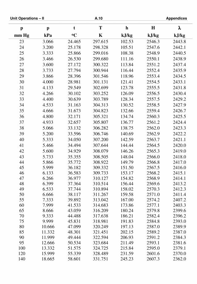
Unit Operations – II A.10 Appendices
p
mm Hg
p
kPa
t
oC
T
K
h
kJ/kg
H
kJ/kg
λλλλ
kJ/kg
23
24
25
26
27
28
29
30
31
32
33
34
35
36
37
38
39
40
41
42
3.066
3.200
3.333
3.466
3.600
3.733
3.866
4.000
4.133
4.266
4.400
4.533
4.666
4.800
4.933
5.066
5.200
5.333
5.466
5.600
24.465
25.178
25.866
26.530
27.172
27.794
28.396
28.981
29.549
30.102
30.639
31.163
31.673
32.171
32.657
33.132
33.596
34.050
34.494
34.929
297.615
298.328
299.016
299.680
300.322
300.944
301.546
301.131
302.699
303.252
303.789
304.313
304.823
305.321
305.807
306.282
306.746
307.200
307.644
308.079
102.53
105.51
108.38
111.16
113.84
116.44
118.96
121.41
123.78
126.09
128.34
130.52
132.66
134.74
136.77
138.75
140.69
142.59
144.44
146.26
2546.3
2547.6
2548.9
2550.1
2551.2
2552.4
2553.4
2554.5
2555.5
2556.5
2557.5
2558.5
2559.4
2560.3
2561.2
2562.0
2562.9
2563.7
2564.5
2565.3
2443.8
2442.1
2440.5
2438.9
2437.4
2435.9
2434.5
2433.1
2431.8
2430.4
2429.2
2427.9
2426.7
2425.5
2424.4
2423.3
2422.2
2421.1
2420.0
2419.0
43
44
45
46
47
48
49
50
55
60
65
70
75
80
85
90
95
100
120
140
5.733
5.866
5.999
6.133
6.266
6.399
6.533
6.666
7.333
7.999
8.666
9.333
9.999
10.666
11.332
11.999
12.666
13.332
15.999
18.665
35.355
35.772
36.182
36.583
36.977
37.364
37.744
38.117
39.892
41.533
43.059
44.488
45.831
47.099
48.301
49.444
50.534
51.575
55.339
58.601
308.505
308.922
309.332
309.733
310.127
310.514
310.894
311.267
313.042
314.683
316.209
317.638
318.981
320.249
321.451
322.594
323.684
324.725
328.489
331.751
148.04
149.79
151.50
153.17
154.82
156.44
158.02
159.58
167.00
173.86
180.24
186.21
191.83
197.13
202.15
206.93
211.49
215.84
231.59
245.23
2566.0
2566.8
2567.5
2568.2
2568.9
2569.6
2570.3
2571.0
2574.2
2577.1
2579.8
2582.4
2584.8
2587.0
2589.2
2591.2
2593.1
2595.0
2601.6
2607.3
2418.0
2417.0
2416.0
2415.1
2414.1
2413.2
2412.3
2411.4
2407.2
2403.3
2399.6
2396.2
2393.0
2389.9
2387.0
2384.3
2381.6
2379.1
2370.0
2362.0
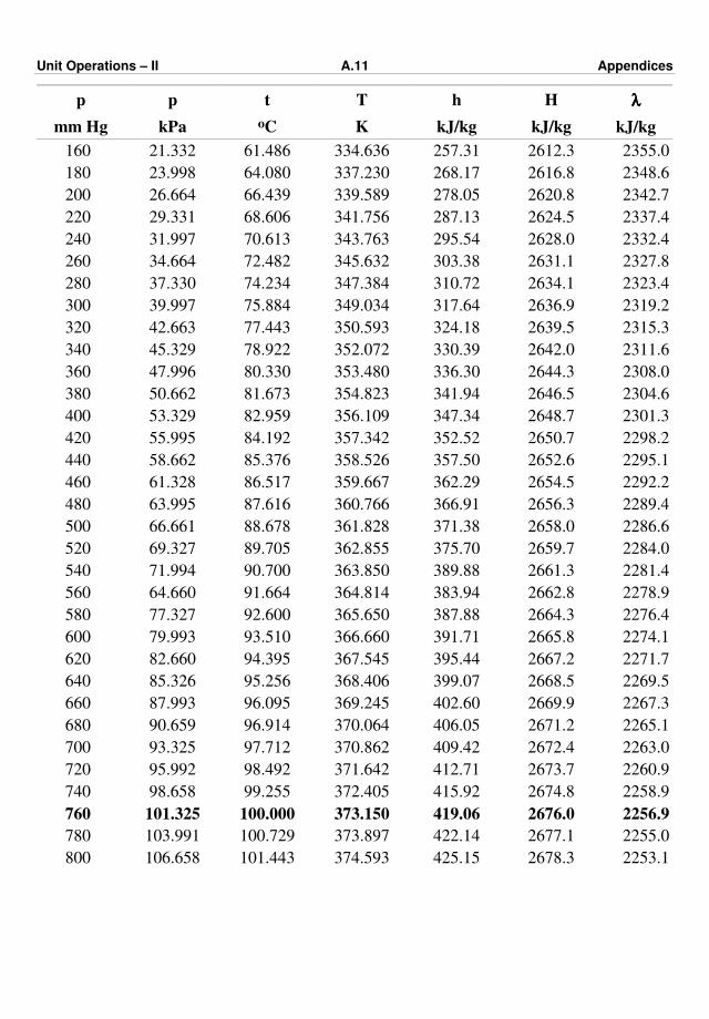
Unit Operations – II A.11 Appendices
p
mm Hg
p
kPa
t
oC
T
K
h
kJ/kg
H
kJ/kg
λλλλ
kJ/kg
160
180
200
220
240
260
280
300
320
340
360
380
400
420
440
460
480
500
520
540
21.332
23.998
26.664
29.331
31.997
34.664
37.330
39.997
42.663
45.329
47.996
50.662
53.329
55.995
58.662
61.328
63.995
66.661
69.327
71.994
61.486
64.080
66.439
68.606
70.613
72.482
74.234
75.884
77.443
78.922
80.330
81.673
82.959
84.192
85.376
86.517
87.616
88.678
89.705
90.700
334.636
337.230
339.589
341.756
343.763
345.632
347.384
349.034
350.593
352.072
353.480
354.823
356.109
357.342
358.526
359.667
360.766
361.828
362.855
363.850
257.31
268.17
278.05
287.13
295.54
303.38
310.72
317.64
324.18
330.39
336.30
341.94
347.34
352.52
357.50
362.29
366.91
371.38
375.70
389.88
2612.3
2616.8
2620.8
2624.5
2628.0
2631.1
2634.1
2636.9
2639.5
2642.0
2644.3
2646.5
2648.7
2650.7
2652.6
2654.5
2656.3
2658.0
2659.7
2661.3
2355.0
2348.6
2342.7
2337.4
2332.4
2327.8
2323.4
2319.2
2315.3
2311.6
2308.0
2304.6
2301.3
2298.2
2295.1
2292.2
2289.4
2286.6
2284.0
2281.4
560
580
600
620
640
660
680
700
720
740
760
780
800
64.660
77.327
79.993
82.660
85.326
87.993
90.659
93.325
95.992
98.658
101.325
103.991
106.658
91.664
92.600
93.510
94.395
95.256
96.095
96.914
97.712
98.492
99.255
100.000
100.729
101.443
364.814
365.650
366.660
367.545
368.406
369.245
370.064
370.862
371.642
372.405
373.150
373.897
374.593
383.94
387.88
391.71
395.44
399.07
402.60
406.05
409.42
412.71
415.92
419.06
422.14
425.15
2662.8
2664.3
2665.8
2667.2
2668.5
2669.9
2671.2
2672.4
2673.7
2674.8
2676.0
2677.1
2678.3
2278.9
2276.4
2274.1
2271.7
2269.5
2267.3
2265.1
2263.0
2260.9
2258.9
2256.9
2255.0
2253.1

Unit Operations – II A.12 Appendices
Table 2 : Properties of saturated water and Dry steam from 0.10 to 14 MPa a
P
MPa
t
°°°°C
T
K
h
kJ/kg
H
kJ/kg λλλλ
kJ/kg
0.10
0.11
0.12
0.13
0.14
0.15
0.16
0.17
0.18
0.19
0.20
0.21
0.22
0.23
0.24
0.25
0.26
0.27
0.28
0.29
99.63
102.32
104.81
107.13
109.32
111.37
113.32
115.17
116.93
118.62
120.23
121.78
123.27
124.71
126.09
127.43
128.73
129.98
131.20
132.39
372.78
375.47
377.96
380.28
382.47
384.52
386.47
388.32
390.08
391.77
393.38
394.93
396.42
397.86
399.24
400.58
401.88
403.13
404.35
405.54
417.51
428.84
439.36
449.19
458.42
467.13
475.38
483.22
490.70
497.85
504.70
511.28
517.62
523.73
529.63
535.34
540.87
546.24
551.44
556.50
2675.4
2679.6
2683.4
2687.0
2690.3
2693.4
2696.2
2699.0
2701.5
2704.0
2706.3
2708.5
2710.6
2712.6
2714.5
2716.4
2718.2
2719.9
2721.5
2723.1
2257.9
2250.9
2244.1
2237.8
2231.9
2226.2
2220.9
2215.7
2210.8
2206.1
2201.6
2197.2
2193.0
2188.9
2184.9
2181.0
2177.3
2173.6
2170.1
2166.6
0.30
0.31
0.32
0.33
0.34
0.35
0.36
0.37
0.38
0.39
0.40
0.41
0.42
0.43
0.44
0.45
0.46
0.47
0.48
0.49
133.54
134.66
135.75
136.82
137.86
138.87
139.86
140.83
141.78
142.71
143.62
144.52
145.39
146.25
147.09
147.92
148.73
149.53
150.31
151.08
406.69
407.81
408.90
409.97
411.01
412.02
413.01
413.98
414.93
415.86
416.77
417.67
418.54
419.40
420.24
421.07
421.88
422.68
423.46
424.23
561.43
566.23
570.90
575.46
579.92
584.27
588.53
592.69
596.76
600.76
604.67
608.51
612.27
615.97
619.60
623.16
626.67
630.11
633.50
636.83
2724.7
2726.1
2727.6
2729.0
2730.3
2731.6
2732.9
2734.1
2735.3
2736.5
2737.6
2738.7
2739.8
2740.9
2741.9
2742.9
2743.9
2744.8
2745.7
2746.6
2163.2
2159.9
2156.7
2153.5
2150.4
2147.4
2144.4
2141.4
2138.6
2135.7
2133.0
2130.2
2127.5
2124.9
2122.3
2119.7
2117.2
2114.7
2112.2
2109.8

Unit Operations – II A.13 Appendices
P
MPa
t
°°°°C
T
K
h
kJ/kg
H
kJ/kg λλλλ
kJ/kg
0.50
0.52
0.54
0.56
0.58
0.60
0.62
0.64
0.66
0.68
0.70
0.72
0.74
0.76
0.78
0.80
0.82
0.84
0.86
0.88
151.84
153.33
154.76
156.16
157.52
158.84
160.12
161.38
162.60
163.79
164.96
166.10
167.21
168.30
169.37
170.41
171.44
172.45
173.44
174.41
424.99
426.48
427.91
429.31
430.67
431.99
433.27
434.53
435.75
436.94
438.11
439.25
440.36
441.45
442.52
443.56
444.59
445.60
446.59
447.56
640.12
646.53
652.76
658.81
664.69
670.42
676.01
681.46
686.78
691.98
697.06
702.03
706.90
711.67
716.35
720.94
725.43
729.85
734.19
738.45
2747.5
2749.3
2750.9
2752.5
2754.0
2755.5
2756.9
2758.2
2759.5
2760.8
2762.0
2763.2
2764.3
2765.4
2766.4
2767.5
2768.5
2769.4
2770.4
2771.3
2107.4
2102.7
2098.1
2093.7
2089.3
2085.0
2080.9
2076.8
2072.7
2068.8
2064.9
2061.1
2057.4
2053.7
2050.1
2046.5
2043.0
2039.6
2036.2
2032.8
0.90
0.92
0.94
0.96
0.98
1.00
1.05
1.10
1.15
1.20
1.25
1.30
1.35
1.40
1.45
1.50
1.55
1.60
1.65
1.70
175.36
176.29
177.21
178.12
179.01
179.88
182.02
184.07
186.05
187.96
189.81
191.61
193.35
195.04
196.69
198.29
199.85
201.37
202.86
204.31
448.51
449.44
450.36
451.27
452.16
453.03
455.17
457.22
459.20
461.11
462.96
464.76
466.50
468.19
469.84
471.44
473.00
474.52
476.01
477.46
742.64
746.76
750.82
754.81
758.74
762.61
772.03
781.12
789.92
798.43
806.69
814.70
822.49
830.07
837.46
844.66
851.69
858.56
865.28
871.84
2772.1
2773.0
2773.8
2774.6
2775.4
2776.2
2778.0
2779.7
2781.3
2782.7
2784.1
2785.4
2786.6
2787.8
2788.9
2789.9
2790.8
2791.7
2792.6
2793.4
2029.5
2026.2
2023.0
2019.8
2016.7
2013.6
2005.9
1998.5
1991.3
1984.3
1977.4
1970.7
1964.2
1957.7
1951.4
1945.2
1939.2
1933.2
1927.3
1921.5

Unit Operations – II A.14 Appendices
P
MPa
t
°°°°C
T
K
h
kJ/kg
H
kJ/kg λλλλ
kJ/kg
1.75
1.80
1.85
1.90
1.95
2.00
2.05
2.10
2.15
2.20
2.25
2.30
2.35
2.40
2.45
2.50
2.55
2.60
2.65
2.70
205.72
207.11
208.47
209.80
211.10
212.37
213.63
214.63
216.06
217.24
218.41
219.55
220.68
221.78
222.87
223.94
225.00
226.04
227.06
228.07
478.87
480.26
481.62
482.95
484.25
485.52
486.78
488.00
489.21
490.39
491.56
492.70
493.83
494.93
496.02
497.09
498.15
499.19
500.21
501.22
878.27
884.57
890.75
896.81
902.75
908.59
914.32
919.96
925.50
930.95
936.32
941.60
946.80
951.93
956.98
961.96
966.87
971.72
976.50
981.22
2794.1
2794.8
2795.5
2796.1
2796.7
2797.2
2797.7
2798.2
2798.6
2799.1
1799.4
2799.8
2800.1
2800.4
2800.7
2800.9
2801.2
2801.4
2801.6
2801.7
1915.9
1910.3
1904.7
1899.3
1893.9
1888.6
1883.4
1878.2
1873.1
1868.1
1863.1
1858.2
1853.3
1848.5
1843.7
1839.0
1834.3
1829.6
1825.1
1820.5
2.75
2.80
2.85
2.90
2.95
3.00
3.10
3.20
3.30
3.40
3.50
3.60
3.70
3.80
3.90
4.00
4.20
4.40
4.60
4.80
229.07
230.05
231.01
231.97
232.91
233.84
235.67
237.45
239.18
240.88
242.54
244.16
245.75
247.31
248.84
250.33
253.24
256.05
258.75
261.37
502.22
503.20
504.16
505.12
506.06
506.99
508.82
510.60
512.33
514.03
515.69
517.31
518.90
520.46
521.99
523.48
526.39
529.20
531.90
534.52
985.88
990.48
995.03
999.52
1003.96
1008.35
1016.99
1025.43
1033.70
1041.81
1049.76
1057.56
1065.21
1072.74
1080.13
1087.40
1101.60
1115.38
1128.76
1141.78
2801.9
2802.0
2802.1
2802.2
2802.2
2802.3
2802.3
2802.3
2802.3
2802.1
2802.0
2801.7
2801.4
2801.1
2800.8
2800.3
2799.4
2798.3
2797.0
2795.7
1816.0
1811.5
1807.1
1802.6
1798.3
1793.9
1785.4
1776.9
1768.6
1760.3
1752.2
1744.2
1736.2
1728.4
1720.6
1712.9
1697.8
1682.9
1668.3
1653.9
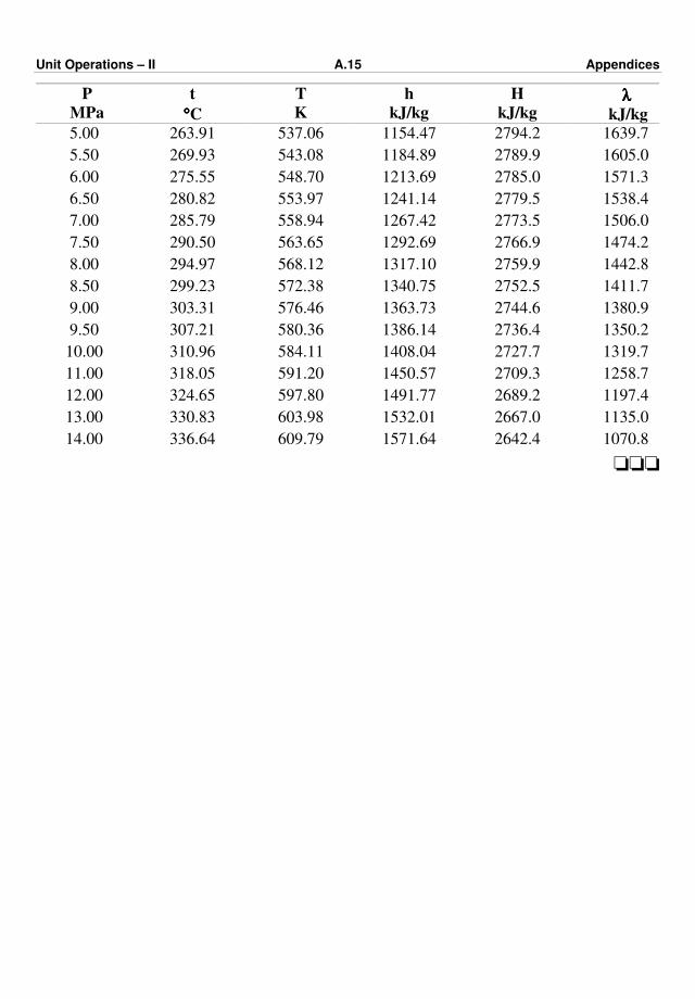
Unit Operations – II A.15 Appendices
P
MPa
t
°°°°C
T
K
h
kJ/kg
H
kJ/kg λλλλ
kJ/kg
5.00
5.50
6.00
6.50
7.00
7.50
8.00
8.50
9.00
9.50
10.00
11.00
12.00
13.00
14.00
263.91
269.93
275.55
280.82
285.79
290.50
294.97
299.23
303.31
307.21
310.96
318.05
324.65
330.83
336.64
537.06
543.08
548.70
553.97
558.94
563.65
568.12
572.38
576.46
580.36
584.11
591.20
597.80
603.98
609.79
1154.47
1184.89
1213.69
1241.14
1267.42
1292.69
1317.10
1340.75
1363.73
1386.14
1408.04
1450.57
1491.77
1532.01
1571.64
2794.2
2789.9
2785.0
2779.5
2773.5
2766.9
2759.9
2752.5
2744.6
2736.4
2727.7
2709.3
2689.2
2667.0
2642.4
1639.7
1605.0
1571.3
1538.4
1506.0
1474.2
1442.8
1411.7
1380.9
1350.2
1319.7
1258.7
1197.4
1135.0
1070.8
ooo


![[PPT]Operations research: An Introduction - Dr. Manoj … · Web viewSyllabi PAPER 6 (ii) : OPERATIONS RESEARCH UNIT-I Operations Research—Meaning, Significance and Scope. Introduction](https://static.documents.pub/doc/80x56/5af27fb47f8b9a8b4c9042ad/pptoperations-research-an-introduction-dr-manoj-viewsyllabi-paper-6-ii.jpg)


