2 Unit Quaternions: A Mathematical Tool for Modeling, Path Planning and Control of Robot Manipulators Ricardo Campa and Karla Camarillo Instituto Tecnológico de la Laguna Mexico 1. Introduction Robot manipulators are thought of as a set of one or more kinematic chains, composed by rigid bodies (links) and articulated joints, required to provide a desired motion to the manipulator’s end–effector. But even though this motion is driven by control signals applied directly to the joint actuators, the desired task is usually specified in terms of the pose (i.e., the position and orientation) of the end–effector. This leads to consider two ways of describing the configuration of the manipulator, at any time (Rooney & Tanev, 2003): via a set of joint variables or pose variables. We call these configuration spaces the joint space and the pose space, respectively. But independently of the configuration space employed, the following three aspects are of interest when designing and working with robot manipulators: • Modeling: The knowledge of all the physical parameters of the robot, and the relations among them. Mathematical (kinematic and dynamic) models should be extracted from the physical laws ruling the robot’s motion. Kinematics is important, since it relates joint and pose coordinates, or their time derivatives. Dynamics, on the other hand, takes into account the masses and forces that produce a given motion. • Task planning: The process of specifying the different tasks for the robot, either in pose or joint coordinates. This may involve from the design and application of simple time trajectories along precomputed paths (this is called trajectory planning), to complex computational algorithms taking real–time decisions during the execution of a task. • Control: The elements that allow to ensure the accomplishment of the specified tasks in spite of perturbances or unmodeled dynamics. According to the type of variables used in the control loop, we can have joint space controllers or pose space controllers. Robot control systems can be implemented either at a low level (e.g. electronic controllers in the servo–motor drives) or via sophisticated high–level programs in a computer. Fig. 1 shows how these aspects are related to conform a robot motion control system. By motion control we refer to the control of a robotic mechanism which is intended to track a desired time–varying trajectory, without taking into account the constraints given by the environment, i.e., as if moving in free space. In such a case the desired task (a time function along a desired path) is generated by a trajectory planner, either in joint or pose variables. The motion controller can thus be designed either in joint or pose space, respectively. www.intechopen.com
Transcript
2
Unit Quaternions: A Mathematical Tool for Modeling, Path Planning and Control of Robot
Manipulators
Ricardo Campa and Karla Camarillo Instituto Tecnológico de la Laguna
Mexico
1. Introduction
Robot manipulators are thought of as a set of one or more kinematic chains, composed by rigid bodies (links) and articulated joints, required to provide a desired motion to the manipulator’s end–effector. But even though this motion is driven by control signals applied directly to the joint actuators, the desired task is usually specified in terms of the pose (i.e., the position and orientation) of the end–effector. This leads to consider two ways of describing the configuration of the manipulator, at any time (Rooney & Tanev, 2003): via a set of joint variables or pose variables. We call these configuration spaces the joint space and the pose space, respectively. But independently of the configuration space employed, the following three aspects are of interest when designing and working with robot manipulators:
• Modeling: The knowledge of all the physical parameters of the robot, and the relations among them. Mathematical (kinematic and dynamic) models should be extracted from the physical laws ruling the robot’s motion. Kinematics is important, since it relates joint and pose coordinates, or their time derivatives. Dynamics, on the other hand, takes into account the masses and forces that produce a given motion.
• Task planning: The process of specifying the different tasks for the robot, either in pose or joint coordinates. This may involve from the design and application of simple time trajectories along precomputed paths (this is called trajectory planning), to complex computational algorithms taking real–time decisions during the execution of a task.
• Control: The elements that allow to ensure the accomplishment of the specified tasks in spite of perturbances or unmodeled dynamics. According to the type of variables used in the control loop, we can have joint space controllers or pose space controllers. Robot control systems can be implemented either at a low level (e.g. electronic controllers in the servo–motor drives) or via sophisticated high–level programs in a computer.
Fig. 1 shows how these aspects are related to conform a robot motion control system. By motion control we refer to the control of a robotic mechanism which is intended to track a desired time–varying trajectory, without taking into account the constraints given by the environment, i.e., as if moving in free space. In such a case the desired task (a time function along a desired path) is generated by a trajectory planner, either in joint or pose variables. The motion controller can thus be designed either in joint or pose space, respectively.
www.intechopen.com
Robot Manipulators
22
Figure 1. General scheme of a robot motion control system
Most of industrial robot manipulators are driven by brushless DC (BLDC) servoactuators. A BLDC servo system is composed by a permanent–magnet synchronous motor, and an electronic drive which produces the required power signals (Krause et al., 2002). An important feature of BLDC drives is that they contain several nested control loops, and they can be configured so as to accept as input for their inner controllers either the motor’s desired position, velocity or torque. According to this, a typical robot motion controller (such as the one shown in Fig. 1) which is expected to include a position tracking control loop, should provide either velocity or torque reference signals to each of the joint actuators’ inner loops. Thus we have kinematic and dynamic motion controllers, respectively. On the other hand, it is a well–known fact that the number of degrees of freedom required to completely define the pose of a rigid body in free space is six, being three for position and three for orientation. In order to do so, we need to attach a coordinate frame to the body and then set the relations between this moving frame and a fixed one (see Fig. 2). Position is well
described by a position vector 3p∈{ , but in the case of orientation there is not a
generalized method to describe it, and this is mainly due to the fact that orientation
constitutes a three–dimensional manifold, 3M , which is not a vector space, but a Lie group.
Figure 2. Position and orientation of a rigid body
Minimal representations of orientation are defined by three parameters, e.g., Euler angles. But in spite of their popularity, Euler angles suffer the drawbacks of representation singularities and inconsistency with the task geometry (Natale, 2003). There are other
nonminimal parameterizations of orientation which use a set of 3 k+ parameters, related by
k holonomic constraints, in order to keep the required three degrees of freedom. Common
examples are the rotation matrices, the angle–axis pair and the Euler parameters. For a list of these and other nonminimal parameterizations of orientation see, e.g., (Spring, 1986). This work focuses on Euler parameters for describing orientation. They are a set of four parameters with a unit norm constraint, so that they can be considered as points lying on the
surface of the unit hypersphere 3 4S ⊂ { . Therefore, Euler parameters are unit quaternions, a
subset of the quaternion numbers, first described by Sir W. R. Hamilton in 1843, as an extension to complex numbers (Hamilton, 1844).
www.intechopen.com
Unit Quaternions: A Mathematical Tool for Modeling, Path Planning and Control of Robot Manipulators
23
The use of Euler parameters in robotics has increased in the latter years. They are an alternative to rotation matrices for defining the kinematic relations among the robot’s joint variables and the end–effector’s pose. The advantage of using unit quaternions over rotation matrices, however, appears not only in the computational aspect (e.g., reduction of floating–point operations, and thus, of processing time) but also in the definition of a proper orientation error for control purposes. The term task space control (Natale, 2003) has been coined for referring to the case of pose control when the orientation is described by unit quaternions, in opposition to the traditional operational space control, which employs Euler angles (Khatib, 1987). Several works have been done using this approach (see, e.g., Lin, 1995; Caccavale et al., 1999; Natale, 2003; Xian et al., 2004; Campa et al., 2006). The aim of this work is to show how unit quaternions can be applied for modeling, path planning and control of robot manipulators. After recalling the main properties of quaternion algebra in Section 2, we review some quaternion–based algorithms that allow to obtain the kinematics and dynamics of serial manipulators (Section 3). Section 4 deals with path planning, and describes two algorithms for generating curves in the orientation manifold. Section 5 is devoted to task–space control. It starts with the specification of the pose error and the control objective, when orientation is given by unit quaternions. Then, two common pose controllers (the resolved motion rate controller and the resolved acceleration controller) are analyzed. Even though these controllers have been amply studied in literature, the Lyapunov stability analysis presented here is novel since it uses a quaternion–based space–state approach. Concluding remarks are given in Section 6.
Throughout this paper we use the notation { }m Aλ and { }M Aλ to indicate the smallest and
largest eigenvalues, respectively, of a symmetric positive definite matrix ( )A x for all
nx ∈ { . The Euclidean norm of vector x is defined as = Tx x x . Also, for a given matrix
A , the spectral norm AE E is defined as { }T
MA A Aλ=E E .
2. Euler Parameters
For the purpose of this work, an n –dimensional manifold Mn m⊆ { , with n m≤ , can be
easily understood as a subset of the Euclidean space m{ containing all the points whose
coordinates 1 2 mx x … x, , , satisfy r m n= − holonomic constraint equations of the form
1 2( ) 0i mx x … xγ , , , = ( 1 2i … r= , , , ). As a typical example of an n –dimensional manifold we have
the generalized unit (hyper)sphere 1Sn n+⊂ { , defined as
1S { 1}n nx x+= ∈ : = .{ E E
It is well–known that the configuration space of a rigid–body’s orientation is a tree–
dimensional manifold, 3M m⊂ { , where m is the number of parameters employed to
describe the orientation. Thus we have minimal ( 3m = ) and non–minimal ( 3m > )
parameterizations of the orientation, being the most common the following:
Given the fixed and body coordinate frames (Fig. 2), Euler angles indicate the sequence of rotations around one of the frame’s axes required to make them coincide with those of the other frame. There are several conventions of Euler angles (depending of the sequence of axes to rotate), but all of them have inherently the problem of singular points, i.e., orientations for which the set of Euler angles is not uniquely defined (Kuipers, 1999). Euler also showed that the relative orientation between two frames with a common origin is equivalent to a single rotation of a minimal angle around an axis passing through the origin. This is known as the Euler’s rotation theorem, and implies that other way of describing
orientation is by specifying the minimal angle θ ∈{ and a unit vector 2 3Su∈ ⊂ {
indicating the axis of rotation. This parameterization, known as the angle/axis pair, is non–minimal since we require four parameters and one holonomic constraint, i.e., the unit norm condition of u .
The angle/axis parameterization, however, has some drawbacks that make difficult its
application. First, it is easy to see that the pairs T
Tuθ⎡ ⎤⎣ ⎦ and 2ST
Tuθ⎡ ⎤− − ∈ ×⎣ ⎦ { both give
the same orientation (in other words, 2S×{ is a double cover of the orientation manifold).
But the main problem is that the angle/axis pair has a singularity when 0θ = , since in such
case u is not uniquely defined.
A most proper way of describing the orientation manifold is by means of an orthogonal
rotation matrix SO(3)R∈ , where the special orthogonal group, defined as
3 3SO(3) { det( ) 1}TR R R I R×= ∈ : = , ={
is a 3–dimensional manifold requiring nine parameters, that is, 3 3 3 9M SO(3) ×≡ ⊂ ≡{ { (it is
easy to show that the matrix equation TR R I= is in fact a set of six holonomic constraints,
and det( ) 1R = is one of the two possible solutions). Furthermore, being SO(3) a
multiplicative matrix group, it means that the composition of two rotation matrices is also a rotation matrix, or
1 2 1 2SO(3) SO(3)R R R R, ∈ ⇒ ∈ .
A group which is also a manifold is called a Lie group. Rotation matrices are perhaps the most extended method for describing orientation, mainly due to the convenience of matrix algebra operations, and because they do not have the problem of singular points, but rotation matrices are rarely used in control tasks due to the difficulty of extracting from them a suitable vector orientation error.
Quaternion numbers (whose set is named H after Hamilton) are considered the immediate extension to complex numbers. In the same way that complex numbers can be seen as arrays
of two real numbers (i.e. 2≡ {C ) with all basic arithmetic operations defined, quaternions
become arrays of four real numbers ( 4≡ {H ). It is useful however to group the last three
components of a quaternion as a vector in 3{ . Thus [ ]Ta b c d ∈H , and T
Ta v⎡ ⎤ ∈⎣ ⎦ H ,
with 3v∈{ , are both valid representations of quaternions ( a is called the scalar part, and v
www.intechopen.com
Unit Quaternions: A Mathematical Tool for Modeling, Path Planning and Control of Robot Manipulators
25
the vector part, of the quaternion). Given two quaternions 1 2,z z ∈H , where [ ]1 1 1
TTz a v=
and [ ]2 2 2
TTz a v= , the following quaternion operations are defined:
• Conjugation:
1*
1
1
az
v
⎡ ⎤= ∈⎢ ⎥−⎣ ⎦ H
• Inversion:
11
1 21
zz
z
∗− = ∈
E EH
where the quaternion Euclidean norm is defined as usual 21 1 1 1 11
TT a v vz z z= = +E E .
• Addition/subtraction:
1 2
1 2
1 2
a az z
v v
±⎡ ⎤± = ∈⎢ ⎥±⎣ ⎦ H
• Multiplication:
1 21 2
1 2
2 1 1 21 2 ( )
Ta a v vz z
a a Sv v v v
⎡ ⎤−⊗ = ∈⎢ ⎥
+ +⎣ ⎦ H (1)
where ( )S ⋅ is a matrix operator such that, for all 3
1 2 3
Tx x x x⎡ ⎤⎢ ⎥⎣ ⎦= ∈{ produces a skew–
symmetric matrix, given by:
3 2
13
2 1
0
( ) 0
0
x x
S x x x
x x
−⎡ ⎤⎢ ⎥= − .⎢ ⎥⎢ ⎥−⎣ ⎦
Skew–symmetric matrices have several useful properties, such as the following (for all 3x y z, , ∈ { ):
( ) ( ) ( )TS x S x S x= − = − , (2)
( )( ) ( ) ( )S x y z S x y S x z+ = + , (3)
( ) ( )S x y S y x= − , (4)
( ) 0S x x = , (5)
( ) 0TS x yy = , (6)
( ) ( )T TS y z S x yx z= , (7)
( ) ( ) T TS x S y y yIx x= − . (8)
www.intechopen.com
Robot Manipulators
26
Note that, by (4), quaternion multiplication is not commutative, that is, 1 2 2 1z z z z⊗ ≠ ⊗ .
• Division: Due to the non–commutativity of the quaternion multiplication, dividing 1z
by 2z can be either
* *11 11 2 2
11 2 22 2
2 2
or .− −⊗ ⊗⊗ = , ⊗ =
E E E Ez z z z
z z z zz z
Euler parameters are another way of describing the orientation of a rigid body. They are
four real parameters, here named η , 1ε , 2ε , 3ε ∈{ , subject to a unit norm constraint, so
that they are points lying on the surface of the unit hypersphere 3 4S ⊂ { . Euler parameters
are also unit quaternions. Let 3Sξ η ε⎡ ⎤= ∈⎣ ⎦TT , with 3
1 2 3
Tε ε ε ε⎡ ⎤⎢ ⎥⎣ ⎦= ∈{ , be a unit
quaternion. Then the unit norm constraint can be written as
2 1ξ η ε ε= + = .E E T (9)
An important property of unit quaternions is that they form a multiplicative group (in fact, a Lie group) using the quaternion multiplication defined in (1). More formally:
The proof of (10) relies in showing that the multiplication result has unit norm, by using (9) and some properties of the skew–symmetric operator. Given the angle/axis pair for a given orientation, the Euler parameters can be easily obtained, since (Sciavicco & Siciliano, 2000):
cos sin2 2
uθ θ
η ε⎛ ⎞ ⎛ ⎞= , = .⎜ ⎟ ⎜ ⎟⎝ ⎠ ⎝ ⎠ (11)
And it is worth noticing that the Euler parameters solve the singularity of the angle/axis
pair when 0θ = . If a rotation matrix { } SO(3)ijR r= ∈ is given, then the corresponding Euler
Conversely, given the Euler parameters 3Sη ε⎡ ⎤ ∈⎣ ⎦TT for a given orientation, the
corresponding rotation matrix SO(3)R∈ can be found as (Sciavicco & Siciliano, 2000):
2( ) ( ) 2 ( ) 2T TR I Sη ε η ε ε η ε εε, = − + + . (13)
However, note in (13) that ( ) ( )R Rη ε η ε, = − ,− , meaning that 3S is a double cover of SO(3) .
That is to say that every given orientation 3Mφ ∈ corresponds to one and only one rotation
www.intechopen.com
Unit Quaternions: A Mathematical Tool for Modeling, Path Planning and Control of Robot Manipulators
27
matrix, but maps into two unit quaternions, representing antipodes in the unit hypersphere (Gallier, 2000):
3SO(3) S⎡ ⎤
∈ ⇔ ± ∈ .⎢ ⎥⎣ ⎦Rη
ε (14)
Also from (13) we can verify that ( ) ( )TR Rη ε η ε,− = , and, as 3ST
Tη ε⎡ − ⎤ ∈⎣ ⎦ is the conjugate
(or inverse) of 3ST
Tη ε⎡ ⎤ ∈⎣ ⎦ , then we have that
3SO(3) S
∗⎡ ⎤ ⎡ ⎤∈ ⇔ ± = ± ∈ .⎢ ⎥ ⎢ ⎥−⎣ ⎦ ⎣ ⎦
TRη η
ε ε
Another important fact is that quaternion multiplication is equivalent to the rotation matrix
multiplication. Thus, if 3
1 2Sξ ξ± ,± ∈ are the Euler parameters corresponding to the rotation
matrices 1 2 SO(3)R R, ∈ , respectively, then:
1 2 1 2⇔ ± ⊗ .R R ξ ξ (15)
Moreover, the premultiplication of a vector 3v∈{ by a rotation matrix SO(3)R∈ produces
a transformed (rotated) vector 3w Rv= ∈{ . The same transformation can be performed with
quaternion multiplication using w vξ ξ ∗= ⊗ ⊗ , where 3Sξ ∈ is the unit quaternion
corresponding to R and quaternions v , ∈w H are formed adding a null scalar part to the
corresponding vectors ( 0T
Tv v⎡ ⎤= ⎣ ⎦ , 0T
Tw w⎡ ⎤= ⎣ ⎦ ). In sum
3 4
1 1
∗∈ ⇔ ⊗ ⊗ ∈ .{ {Rv vξ ξ (16)
In the case of a time–varying orientation, we need to establish a relation between the time
derivatives of Euler parameters 4T
Tξ η ε⎡ ⎤= ∈⎣ ⎦$ $ $ { and the angular velocity of the rigid body
3ω ∈{ . That relation is given by the so–called quaternion propagation rule (Sciavicco &
Siciliano, 2000):
1( )
2Eξ ξ ω= .$ (17)
where
4 3( ) ( )( )
T
E EI S
εξ η εη ε
×⎡ − ⎤= , = ∈ .⎢ ⎥
−⎣ ⎦ { (18)
By using properties (2), (8) and the unit norm constraint (9) it can be shown that
( ) ( )TE E Iξ ξ = , so that ω can be resolved from (17) as
2 ( )TEω ξ ξ= $ (19)
www.intechopen.com
Robot Manipulators
28
3. Robot Kinematics and Dynamics
Serial robot manipulators have an open kinematic chain, i.e., there is only one path from one end (the base) to the other (the end–effector) of the robotic chain (see Fig. 3). A serial manipulator with n joints, either translational (prismatic) or rotational, has n degrees of
freedom (dof). This section deals only with the modeling of serial manipulators. As explained in (Craig, 2005), any serial robot manipulator can be described by using four
parameters for each joint, that is, a total of 4n parameters for a n –dof manipulator. Denavit
and Hartenberg (Denavit & Hartenberg, 1955) proposed a general method to establish those
parameters in a systematic way, by defining 1n + coordinate frames, one per each link,
including the base. The four Denavit–Hartenberg (or simply D–H) parameters for the i -th
joint can then be extracted from the relation between frame 1i − and frame i , as follows:
ia : Distance from axis 1iz − to iz , along axis ix .
iα : Angle between axes 1iz − and iz , about axis ix .
id : Distance from axis 1ix − to ix , along axis 1iz − .
iθ : Angle between axes 1ix − and ix , about axis 1iz − .
Note that there are three constant D–H parameters for each joint; the other one ( iθ for
rotational joints, id for translational joints) describes the motion produced by such i -th
joint. To follow the common notation, let iq be the variable D–H parameter corresponding
to the i –th joint. Then the so–called joint configuration space is specified by the vector
1 2
T n
nq q q q⎡ ⎤⎢ ⎥⎣ ⎦= ∈ ,A {
while the pose (position and orientation) of the end–effector frame with respect to the base frame (see Fig. 3), denoted here by x , is given by a point in the 6–dimensional pose
configuration space 3 3M×{ , using whichever of the representations for 3M m⊂ { . That is
3 3 3M mp
xφ
+⎡ ⎤= ∈ × ⊂ .⎢ ⎥⎣ ⎦ { {
Figure 3. A 4-dof serial robot manipulator
www.intechopen.com
Unit Quaternions: A Mathematical Tool for Modeling, Path Planning and Control of Robot Manipulators
29
3.1 Direct Kinematics
The direct kinematics problem consists on expressing the end–effector pose x in terms of
q . That is, to find a function (called the kinematics function) 3 3: Mnh → ×{ { such that
( )
( ) .( )
p qx h q
qφ⎡ ⎤
= = ⎢ ⎥⎣ ⎦ (20)
Traditionally, direct kinematics is solved from the D–H parameters using homogeneous matrices (Denavit & Hartenberg, 1955). A homogeneous matrix combines a rotation matrix
and a position vector in an extended 4 4× matrix. Thus, given 3p∈ { and SO(3)R∈ , the
corresponding homogeneous matrix T is
4 4SE(3)0 1T
R pT ×⎡ ⎤
= ∈ ⊂ .⎢ ⎥⎣ ⎦ { (21)
SE(3) is known as the special Euclidean group and contains all homogeneous matrices of the
form (21). It is a group under the standard matrix multiplication, meaning that the product
of two homogeneous matrices 1 2 SE(3)T T, ∈ is given by
2 1 2 1 22 1 1 22 1 SE(3)
0 1 0 1 0 1T T T
R R R R Rp p p pT T
+⎡ ⎤ ⎡ ⎤ ⎡ ⎤= = ∈ .⎢ ⎥ ⎢ ⎥ ⎢ ⎥⎣ ⎦ ⎣ ⎦ ⎣ ⎦ (22)
In terms of the D–H parameters, the relative position vector and rotation matrix of the i -th
frame with respect to the previous one are (Sciavicco & Siciliano, 2000):
1 1 3SO(3)
0
i i i ii i
i i i i i i
ii
i
i i
ii i
i
C S C S S a C
R S C C C S aSp
S C d
θ α θ αθ θ
θ θ α θ α θ
αα
⎡ ⎤⎢ ⎥⎢ ⎥⎢ ⎥⎢ ⎥⎢ ⎥⎢ ⎥⎢ ⎥⎢ ⎥⎢ ⎥⎢ ⎥⎢ ⎥⎣ ⎦
⎡ ⎤⎢ ⎥⎢ ⎥− − ⎢ ⎥⎢ ⎥⎢ ⎥⎢ ⎥⎢ ⎥⎣ ⎦
−
= − ∈ , = ∈ .{ (23)
where xC , xS stand for cos( )x , sin( )x , respectively.
The original method proposed by (Denavit & Hartenberg, 1955) uses the expressions in (23)
to form relative homogeneous matrices 1i
iT− (each depending on iq ), and then the
composition rule (22) to compute the homogeneous matrix of the end–effector with respect
to the base frame, ( ) SE(3)T q ∈ :
0 1 1
1 2
( ) ( )( ) SE(3)
0 1
n
nT
R q p qT q T T T−⎡ ⎤
= = ∈ .⎢ ⎥⎣ ⎦ A
This leads to the following general expressions for the pose of the end–effector, in terms of
( )p q and ( )R q
0 1 1
1 2( ) n
nR q R R R−= A (24)
0 1 2 1 0 1 3 2 2 1 0
1 2 1 1 2 2 11 2 1( ) n n n n
n nn np q R R R R R R … Rp p p p
− − − −− − −= + + + +A A (25)
An alternative method for computing the direct kinematics of serial manipulators using quaternions, instead of homogeneous matrices, was proposed recently by (Campa et al.,
www.intechopen.com
Robot Manipulators
30
2006). The method is inspired in one found in (Barrientos et al. 1997), but it is more general,
and gives explicit expressions for the position 3( )p q ∈{ and orientation 3 4( ) Sqξ ∈ ⊂ { in
terms of the original D–H parameters.
Let us start from the expressions for 1i
iR− and 1i
ip
− in (23). We can use (12) and some
trigonometric identities to obtain the corresponding quaternion 1i
Then, we can apply properties (15) and (16) iteratively to obtain expressions equivalent to (24) and (25):
0 1 1
1 2
0 1 2 1 0 1 2
1 2 1 1 2 1
0 1 3 2 0 1 3 0 1 0 * 0
1 2 2 1 1 2 2 1 2 1 1
( )
( ) ( ) ( )
( ) ( ) .
n
n
n n n
n n n
n n n
n n n
q
p q p
p p p
ξ ξ ξ ξ
ξ ξ ξ ξ ξ ξ
ξ ξ ξ ξ ξ ξ ξ ξ
−
− − − ∗− −
− − − ∗− − −
= ⊗ ⊗ ⊗ ,
= ⊗ ⊗ ⊗ ⊗ ⊗ ⊗ ⊗ ⊗ +
⊗ ⊗ ⊗ ⊗ ⊗ ⊗ ⊗ ⊗ + + ⊗ +
A
A A
A A …
( )qξ is the unit quaternion (Euler parameters) expressing the orientation of the end–effector
with respect to the base frame. The position vector ( )p q is the vector part of the quaternion
( )p q .
An advantage of the proposed method is that the position and orientation parts of the pose are processed separately, using only quaternion multiplications, which are computationally more efficient than homogeneous matrix multiplications. Besides, the result for the orientation part is given directly as a unit quaternion, which is a requirement in task space controllers (see Section 5). The inverse kinematics problem, on the other hand, consists on finding explicit expressions for computing the joint coordinates, given the pose coordinates, that is equivalent to find the
inverse funcion of h in (20), mapping 3 3M×{ to n{ :
1( )q xh−= . (26)
The inverse kinematics, however, is much more complex than direct kinematics, and is not derived in this work.
3.2 Differential Kinematics
Differential kinematics gives the relationship between the joint velocities and the corresponding end–effector’s linear and angular velocities (Sciavicco & Siciliano, 2000).
www.intechopen.com
Unit Quaternions: A Mathematical Tool for Modeling, Path Planning and Control of Robot Manipulators
31
Thus, if = ∈$ {nd
dtq q is the vector of joint velocities, 3v∈{ is the linear velocity, and 3ω ∈{
is the angular velocity of the end–effector, then the differential kinematics equation is given by
( )
( )( )
p
o
J qvq J q q
J qω
⎡ ⎤⎡ ⎤= =⎢ ⎥⎢ ⎥⎣ ⎦ ⎣ ⎦ $ $ (27)
where matrix 6( ) nJ q ×∈ { is the geometric Jacobian of the manipulator, which depends on its
configuration. ( )pJ q , 3( ) n
oJ q ×∈{ are the components of the geometric Jacobian producing
the translational and rotational parts of the motion. Now consider the time derivative of the generic kinematics function (20):
( )
( )( )
( )A
p q
qh qx q q J q q
qq
q
φ
∂⎡ ⎤⎢ ⎥∂∂ ⎢ ⎥= = = .⎢ ⎥∂∂ ⎢ ⎥∂⎣ ⎦$ $ $ $ (28)
Matrix (3 )( ) m n
AJ q + ×∈{ is known as the analytic Jacobian of the robot, and it relates the joint
velocities with the time derivatives of the pose coordinates (or pose velocities).
In the particular case of using Euler parameters for the orientation, 3 4( ) ( ) Sq qφ ξ= ∈ ⊂ { ,
and 7( ) ( ) n
A AJ q J qξ
×= ∈{ , i.e.
( )A
px J q q
ξξ⎡ ⎤
= = .⎢ ⎥⎣ ⎦$
$ $$ (29)
The linear velocity v of the end–effector is simply the time derivative of the position vector
p (i.e. v p= $ ); instead, the angular velocity ω is related with ξ$ by (19). So, we have
( )R
v pJ q
ξω ξ⎡ ⎤ ⎡ ⎤
=⎢ ⎥ ⎢ ⎥⎣ ⎦ ⎣ ⎦$$ (30)
where the representation Jacobian, for the case of using Euler parameters, is defined as
6 70
( )0 2 ( ( ))
R T
IJ q
E qξ ξ
⎡ ⎤⎢ ⎥ ×⎢ ⎥⎢ ⎥⎣ ⎦= ∈{ (31)
with matrix ( )E ξ as in (18). Also notice, by combining (27), (29), and (30), that
( ) ( ) ( )R AJ q J q J qξ ξ
=
Whichever the Jacobian matrix be (geometric, analytic, representation), it is often required to find its inverse mapping, although this is possible only if such a matrix has full rank. In the
case of a matrix n mJ ×∈{ , with n m> , then there exists a left pseudoinverse matrix of J , † m nJ ×∈{ , defined as
( )
1† T TJ J J J
−=
www.intechopen.com
Robot Manipulators
32
such that † m mJ J I ×= ∈ { . On the contrary, if n m< , then there exist a right pseudoinverse
matrix of J , † m nJ ×∈{ , defined as
1† T TJ J JJ
−⎛ ⎞⎜ ⎟⎝ ⎠=
such that † n nJ J I ×= ∈{ . It is easy to show that in the case n m= (square matrix) then † † 1J J J −= = .
3.3 Lagrangian Dynamics
Robot kinematics studies the relations between joint and pose variables (and their time derivatives) during the motion of the robot’s end–effector. These relations, however, are established using only a geometric point of view. The effect of mechanical forces (either external or produced during the motion itself) acting on the manipulator is studied by robot dynamics. As pointed out by (Sciavicco & Siciliano, 2000), the derivation of the dynamic model of a manipulator plays an important role for simulation, analysis of manipulator structures, and design of control algorithms. There are two general methods for derivation of the dynamic equations of motion of a manipulator: one method is based on the Lagrange formulation and is conceptually simple and systematic; the other method is based on the Newton–Euler formulation and allows obtaining the model in a recursive form, so that it is computationally more efficient. In this section we consider the application of the Lagrangian formulation for obtaining the robot dynamics in the case of using Euler parameters for describing the orientation. This approach is not new, since it has been employed for modeling the dynamics of rigid bodies (see, e.g., Shivarama & Fahrenthold, 2004; Lu & Ren, 2006, and references therein). An important fact is that Lagrange formulation allows to obtain the dynamic model independently of the coordinate system employed to describe the motion of the robot. Let us consider a serial robot manipulator with n degrees of freedom. Then we can choose any set
of m n k= + coordinates, say mρ ∈{ , with 0k ≥ holonomic constraints of the form
( ) 0iγ ρ = ( 1 2i … k= , , , ), to obtain the robot’s dynamic model. If 0k = we talk of independent
or generalized coordinates, if 1k ≥ we have dependent or constrained coordinates.
The next step is to express the total (kinetic and potential) energy of the mechanical system
in terms of the chosen coordinates. Let ( )ρ ρ, $K be the kinetic energy, and ( )ρU the
potential energy of the system; then the Lagrangian function ( )ρ ρ, $L is defined as
( ) ( ) ( )ρ ρ ρ ρ ρ, = , −$ $L K U
The Lagrange’s dynamic equations of motion, for the general case (with constraints), are expressed by
( ) ( ) ( )⎧ ⎫ ⎛ ⎞∂ , ∂ , ∂
− = +⎨ ⎬ ⎜ ⎟∂ ∂ ∂⎩ ⎭ ⎝ ⎠
$ $$
T
d
dtρ
ρ ρ ρ ρ γ ρλτ
ρ ρ ρ
L L (32)
where mρτ ∈ { is the vector of (generalized or constrained) forces associated with each of
the coordinates ρ , vector ( )γ ρ is defined as
www.intechopen.com
Unit Quaternions: A Mathematical Tool for Modeling, Path Planning and Control of Robot Manipulators
33
γ ρ
γ ρ γ ργ ρ
ρ
γ ρ
×
⎡ ⎤⎢ ⎥∂⎢ ⎥= ∈ , ∈⎢ ⎥ ∂⎢ ⎥⎣ ⎦
{ {B
1
2
( )
( ) ( )( ) so that
( )
k k m
k
and kλ ∈{ is the vector of k Lagrange multipliers, which are employed to reduce the
dimension of the system, producing only n independent equations in terms of a new set nr∈{ of generalized coordinates. In sum, a general constrained system such as (32), with n kρ +∈{ , can be transformed in an unconstrained system of the form
( ) ( )
r
d r r r r
dt r rτ
∂ , ∂ ,⎧ ⎫− =⎨ ⎬
∂ ∂⎩ ⎭$ $
$L L
(33)
Moreover, as explained by (Spong et al., 2006), equation (33) can be rewritten as:
( ) ( ) ( )r r rrM r r C r r r rg τ+ , + =$$ $ $
where ( ) n n
rM r ×∈{ is a symmetric positive definite matrix known as the inertia matrix,
( ) n n
rC r r ×, ∈$ { is the matrix of centripetal and Coriolis forces, and ( ) n
rrg ∈{ is the vector of
forces due to gravity. These matrices satisfy the following useful properties (Kelly et al., 2005):
• Inertia matrix is directly related to kinetic energy by
1
( ) ( )2
Trr r M r rr, =$ $$K (34)
• For a given robot, matrix ( )rC r r, $ is not unique, but it can always be chosen so that
( ) 2 ( )r rM r C r r− ,$ $ be skew–symmetric, that is
( ) 2 ( ) 0 nT
r rM r C r r x x r rx ⎡ ⎤− , = , ∀ , , ∈⎣ ⎦$ $ $ { (35)
• The vector of gravity forces is the gradient of the potential energy, that is
( )
( )r
rrg
r
∂=
∂
U (36)
Now consider the total mechanical energy of the robot ( ) ( ) ( )r r r r r, = , +$ $E K U . Using
properties (34)–(36), it can be shown that the following relation stands
( ) T
rr r r τ, = .$ $ $E (37)
And, as the rate of change of the total energy in a system is independent of the generalized coordinates, we can use (37) as a way of convert generalized forces between two different generalized coordinate systems.
www.intechopen.com
Robot Manipulators
34
For an n –dof robot manipulator, it is common to express the dynamic model in terms of the
joint coordinates, i.e. nr q≡ ∈{ , this leads us to the well–known equation (Kelly et al., 2005):
Subindexes have been omitted in this case for simplicity; τ is the vector of joint forces (and
torques) applied to each of the robot joints.
Now consider the problem of modeling the robot dynamics of a non–redundant ( 6n ≤ )
manipulator, in terms of the pose coordinates of the end–effector, given by
3 3 7ST
T Tx p ξ⎡ ⎤= ∈ × ⊂⎣ ⎦ { { . Notice that in this case we have holonomic constraints. If 6n =
then the only constraint is given by (9), so that:
2( ) 1Txγ η ε ε= + − ;
If 6n < then the pose coordinates require 6 n− additional constraints to form the vector 7( ) nxγ −∈{ The equations of motion would be
7( )( ) ( ) ( ) ( )
T
x x x xx
xM x x C x x x x x x xg
x
γτ λ τ
∂+ , + = + , , , , ∈ ,
∂$$ $ $ $ $$ { (39)
where matrices ( )xM x , ( )xC x x, , ( )xxg can be computed from ( )M q , ( )C q q, , ( )g q in (38)
using a procedure similar to the one presented in (Khatib, 1987) for the case of operational space. We get
1
1
1
† †
( )
† † † † †
( )
†
( )
( ) ( ( ) ) ( ) ( )
( ) ( ( ) ) ( ( ) ) ( ) ( ( ) ) ( ) ( )
( ) ( ( ) ) ( )
T
x A Aq h x
T Tx AA A A A
q h x
T
Axq h x
M x J q M q J q
C x x J q C q J q x J q J q M q qJ
x J q g qg
ξ ξ
ξξ ξ ξ ξ
ξ
−
−
−
=
=
=
=
, = , +
=
$ $$
where ( )AJ qξ
is the analytic Jacobian in (29). To obtain the previous equations we are
assuming, according to (37), that
( )TT T T
x A xq x J qqξ
τ τ τ= =$ $ $
so that
1
†
( )( ( ) )Tx A
q h xJ q
ξττ
−== .
Equation (39) expresses the dynamics of a robot manipulator in terms of the pose
coordinates ( p , ξ ) of the end–effector. In fact, these are a set of seven equations which can
be reduced to n , by using the 7 n− Lagrange multipliers and choosing a subset of n
www.intechopen.com
Unit Quaternions: A Mathematical Tool for Modeling, Path Planning and Control of Robot Manipulators
35
generalized coordinates taken from x . This procedure, however, can be far complex, and
sometimes unsolvable in analytic form. In theory, we can use (32) to find a minimal system of equations in terms of any set of generalized coordinates. For example, we could choose the scalar part of the Euler
parameters in each joint, iη , ( 1 2i … n= , , , ) as a possible set of coordinates. To this end, it is
useful to recall that the kinetic energy of a free–moving rigid body is a function of the linear and angular velocities of its center of mass, v and ω , respectively, and is given by
1 1
( )2 2
T Tv mv v Hω ω ω, = + ,K (40)
where m is the mass, and H is the matrix of moments of inertia (with respect to the center
of mass) of the rigid body. The potential energy depends only on the coordinates of the center of mass, p , and is given by
( ) ,T
p m pg=U
where g is the vector of gravity acceleration. Now, using (30), (31), we can rewrite (40) as
1
( ) 2 ( ) ( )2
TT Tp m p E HEpξ ξ ξ ξ ξξ, , = +$ $$$ $$K (41)
Considering this, we propose the following procedure to compute the dynamic model of robot manipulators in terms of any combination of pose variables in task space:
1. Using (41), find the kinetic and potential energy of each of the manipulator’s links, in terms of the pose coordinates, as if they were independent rigid bodies. That is,
for link i , compute ( )i ii ip ξ ξ, , $$K and ( ).i i
pU
2. Still considering each link as an independent rigid body, compute the total Lagrangian function of the n –dof manipulator as
1
( , , ) ( ) ( )n
i i iii i
i
p p p pξ ξ ξξ=
⎡ ⎤, = , , −⎣ ⎦∑$ $$ $L K U
where 7nρ ∈{ is a vector containing the pose coordinates of each link, i.e.
ρξ
⎡ ⎤⎢ ⎥ ⎡ ⎤⎢ ⎥= , = ⎢ ⎥⎢ ⎥ ⎣ ⎦⎢ ⎥⎣ ⎦B
1
2with i
i
i
n
x
pxx
x
3. Now use (9), for each joint, and the knowledge of the geometric relations between
links to find 6n holonomic constraints, in order to form vector 6( ) .nγ ρ ∈{
4. Write the constrained equations of motion for the robot, i. e. (32).
5. Finally, solve for the 6n Lagrange multipliers, and get de reduced (generalized)
system in terms of the chosen n generalized coordinates.
www.intechopen.com
Robot Manipulators
36
This procedure, even if not simple (specially for robots with 3n > ) can be useful when
requiring explicit equations for the robot dynamics in other than joint coordinates.
4. Path Planning
The minimal requirement for a manipulator is the capability to move from an initial posture to a final assigned posture. The transition should be characterized by motion laws requiring the actuators to exert joint forces which do not violate the saturation limits and do not excite typically unmodeled resonant modes of the structure. It is then necessary to devise planning algorithms that generate suitably smooth trajectories (Sciavicco & Siciliano, 2000). To avoid confusion, a path denotes simply a locus of points either in joint or pose space; it is a pure geometric description of motion. A trajectory, on the other hand, is a path on which a time law is specified (e.g., in terms of velocities and accelerations at each point of the path). This section shows a couple of methods for designing paths in the task space, i.e., when using Euler parameters for describing orientation. Generally, the specification of a path for a given motion task is done in pose space. It is much easier for the robot’s operator to define a desired position and orientation of the end–effector than to compute the required joint angles for such configuration. A time–varying
position ( )p t is also easy to define, but the same is not valid for orientation, due to the
difficulty of visualizing the orientation coordinates. Of the four orientation parameterizations mentioned in Section 2, perhaps the more intuitive is the angle/axis pair. To reach a new orientation from the actual one, employing a minimal
displacement, we only need to find the required axis of rotation 2Su∈# and the
corresponding angle to rotate θ ∈# { . Given the Euler parameters for the initial orientation,
[ ] 3Sη ε ∈T
To o
, and the desired orientation, [ ] 3Sη ε ∈T
Td d
, it can be shown, using (11) and
quaternion operations, that (Campa & de la Torre, 2006):
# ( ) ( )2arccos
( )
d o o dT o do do d
d o o do d
Su
S
η ηε ε ε εθ η η ε εη ηε ε ε ε
− += + , =
− +#
E E (42)
We can use expressions in (42) to define the minimal path between the initial and final
orientations. A velocity profile can be employed for θ# in order to generate a suitable ( )tθ .
However, during a motion along such a path, it is important that #u remains fixed. Also
notice that when the desired orientation coincides with the initial (i.e., o dη η= , o dε ε= ), then
# 0θ = and u# is not well defined.
Now consider the possibility of finding a path between a given set of points in the task space using interpolation curves. The simplest way of doing so is by means of linear interpolation.
Let the initial pose be given by T
T T
oop ξ⎡ ⎤⎣ ⎦ and the final pose by T
T T
ddp ξ⎡ ⎤⎣ ⎦ , and assume, for
simplicity, that the time required for the motion is normalized, that is, we need to find a
Unit Quaternions: A Mathematical Tool for Modeling, Path Planning and Control of Robot Manipulators
37
For the position part of the motion, the linear interpolation is simply given by
( ) (1 )o d
p t t tp p= − +
but for the orientation part we can not apply the same formula, because, as unit quaternions
do not form a vector space, then such ( )tξ would not be a unit quaternion anymore.
Shoemake (1985) solved this by defining a spherical linear interpolation, or simply slerp, which is given by the following expression
sin([1 ] ) sin( )
( )sin( )
o dt t
tξ ξ
ξ− Ω + Ω
=Ω
(43)
where 1cos ( )T
o dξ ξ−Ω = .
It is possible to show (Dam et al., 1998) that such ( )tξ in (43) satisfies that 3( ) Stξ ∈ , for all
0 1t≤ ≤ . (Dam et al., 1998) is also a good reference for understanding other types of
interpolation using quaternions, including the so called spherical spline quaternion interpolation or squad, which produces smooth curves joining a series of points in the orientation manifold. Even though these algorithms have been used in the fields of computer graphics and animation for years, as far as the authors’ knowledge, there are few works using them for motion planning in robotics.
5. Task-space Control
As pointed out by (Sciavicco & Siciliano, 2000), the joint space control is sufficient in those cases where it is required motion control in free space; however, for the most common applications of interaction control (robot interacting with the environment) it is better to use the so–called task space control (Natale,2003). Thus, in the later years, more research has been done in this kind of control schemes. Euler parameters have been employed in the later years for the control of generic rigid bodies, including spaceships and underwater vehicles. The use of Euler parameters in robot control begins with Yuan (1988) who applied them to a particular version of the resolved–acceleration control (Luh et al., 1980). More recently, several works have been published on this topic (see, e.g., Lin, 1995; Caccavale et al., 1999; Natale, 2003; Xian et al., 2004; Campa et al., 2006, and references therein). The so–called hierarchical control of manipulators is a technique that solves the problem of motion control in two steps (Kelly & Moreno-Valenzuela, 2005): first, a task space kinematic control is used to compute the desired joint velocities from the desired pose trajectories; then, those desired velocities become the inputs for an inner joint velocity control loop (see Fig. 4). This two–loop control scheme was first proposed by Aicardi et al. (1995) in order to solve the pose control problem using a particular set of variables to describe the end–effector orientation. The term kinematic controller (Caccavale et al., 1999) refers to that kind of controller whose output signal is a joint velocity and is the first stage in a hierarchical scheme. On the other hand dynamic controller is employed here for those controllers also including a position controller but producing joint torque signals.
www.intechopen.com
Robot Manipulators
38
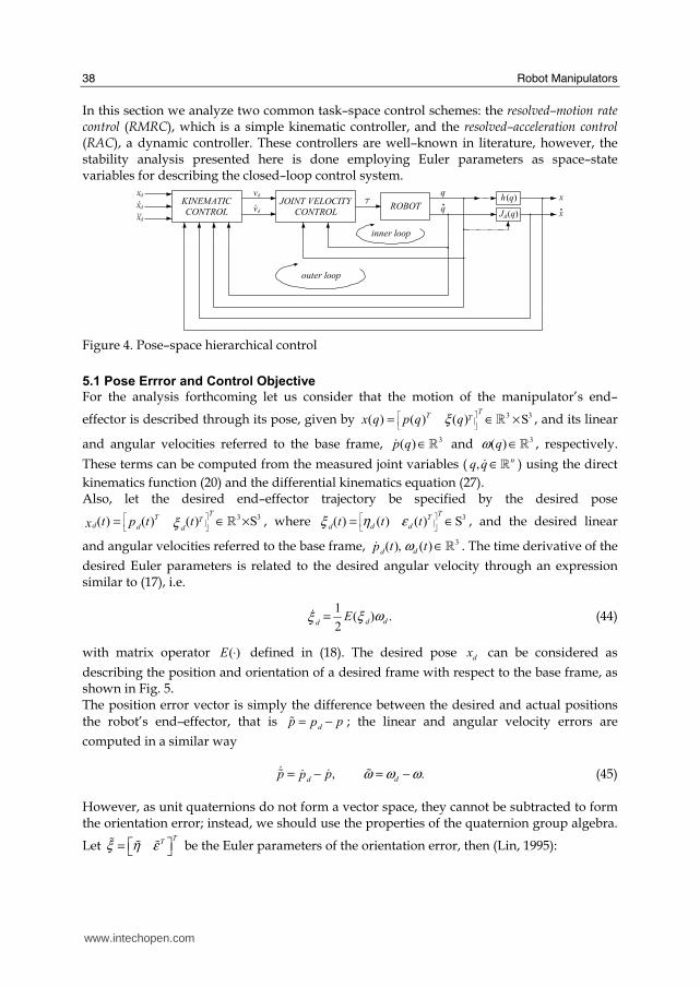
In this section we analyze two common task–space control schemes: the resolved–motion rate control (RMRC), which is a simple kinematic controller, and the resolved–acceleration control (RAC), a dynamic controller. These controllers are well–known in literature, however, the stability analysis presented here is done employing Euler parameters as space–state variables for describing the closed–loop control system.
Figure 4. Pose–space hierarchical control
5.1 Pose Errror and Control Objective
For the analysis forthcoming let us consider that the motion of the manipulator’s end–
effector is described through its pose, given by 3 3( ) ( ) ( ) ST
T Tx q p q qξ⎡ ⎤⎢ ⎥⎣ ⎦= ∈ ×{ , and its linear
and angular velocities referred to the base frame, 3( )p q ∈$ { and 3( )qω ∈{ , respectively.
These terms can be computed from the measured joint variables ( , ∈$ {nq q ) using the direct
kinematics function (20) and the differential kinematics equation (27). Also, let the desired end–effector trajectory be specified by the desired pose
3 3( ) ( ) ( ) ST
T Td d dt t tpx ξ
⎡ ⎤⎢ ⎥⎣ ⎦= ∈ ×{ , where 3( ) ( ) ( ) ST
T
d ddt t tη εξ ⎡ ⎤⎢ ⎥⎣ ⎦= ∈ , and the desired linear
and angular velocities referred to the base frame, 3( ) ( )ddt tp ω, ∈$ { . The time derivative of the
desired Euler parameters is related to the desired angular velocity through an expression similar to (17), i.e.
1( )
2ddd
E ωξξ = .$ (44)
with matrix operator ( )E ⋅ defined in (18). The desired pose dx can be considered as
describing the position and orientation of a desired frame with respect to the base frame, as shown in Fig. 5. The position error vector is simply the difference between the desired and actual positions
the robot’s end–effector, that is d
p pp= −# ; the linear and angular velocity errors are
computed in a similar way
ddp pp ω ω ω= − , = − .$ ## $$ (45)
However, as unit quaternions do not form a vector space, they cannot be subtracted to form the orientation error; instead, we should use the properties of the quaternion group algebra.
Let T
Tξ η ε⎡ ⎤= ⎣ ⎦# # # be the Euler parameters of the orientation error, then (Lin, 1995):
www.intechopen.com
Unit Quaternions: A Mathematical Tool for Modeling, Path Planning and Control of Robot Manipulators
39
d
d
d
η ηξ ξ ξ
εε
∗ ⎡ ⎤ ⎡ ⎤= ⊗ = ⊗⎢ ⎥ ⎢ ⎥−⎣ ⎦⎣ ⎦
#
and applying (1) we get (Sciavicco & Siciliano, 2000):
3S( )
Tdd
d dd S
η ηη ε εξ
ε η η ε εε ε
⎡ ⎤+⎡ ⎤= = ∈ .⎢ ⎥⎢ ⎥ − +⎣ ⎦ ⎣ ⎦
###
(46)
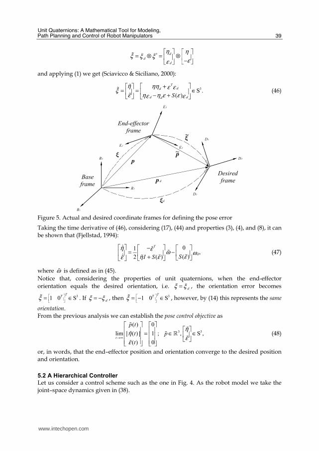
Figure 5. Actual and desired coordinate frames for defining the pose error
Taking the time derivative of (46), considering (17), (44) and properties (3), (4), and (8), it can be shown that (Fjellstad, 1994):
01
( )2 ( )
T
dSI S
η ε ω ωεη εε
⎡ ⎤ ⎡ − ⎤ ⎡ ⎤= − ,⎢ ⎥ ⎢ ⎥ ⎢ ⎥+ ⎣ ⎦⎣ ⎦⎣ ⎦
$# # #$ ## ## (47)
where ω# is defined as in (45).
Notice that, considering the properties of unit quaternions, when the end-effector
orientation equals the desired orientation, i.e. d
ξ ξ= , the orientation error becomes
31 0 ST
Tξ ⎡ ⎤⎢ ⎥⎣ ⎦= ∈# . If d
ξ ξ= − , then 31 0 ST
Tξ ⎡ ⎤⎢ ⎥⎣ ⎦= − ∈# , however, by (14) this represents the same
orientation. From the previous analysis we can establish the pose control objective as
or, in words, that the end–effector position and orientation converge to the desired position and orientation.
5.2 A Hierarchical Controller
Let us consider a control scheme such as the one in Fig. 4. As the robot model we take the joint–space dynamics given in (38).
www.intechopen.com
Robot Manipulators
40
The RMRC is a kinematic controller first proposed by Whitney (1969) to handle the problem
of motion control in operational space via joint velocities (rates). Let 6
dx x, ∈{ be the actual
and desired operational coordinates, respectively, so that dx x x= −# is the pose error in
operational space. The RMRC controller is given by
[ ]†( )d A d xJ q x K xv = +$ # (49)
where † 6( ) n
AJ q ×∈{ is the left pseudoinverse of the analytic Jacobian in (28), n n
xK×∈{ is a
positive definite matrix, and ndv ∈{ is the vector of (resolved) desired joint velocities. In
fact, in the ideal case where dx x= , then 0x =# and we have the inverse analytic Jacobian
mapping. In the case of using Euler parameters, then T
T Tx p ξ⎡ ⎤= ⎣ ⎦ ,
TT T
d ddpx ξ⎡ ⎤= ⎣ ⎦ , and we
can use (Campa et al., 2006):
†( )pd
d
d o
K ppv J q
Kω ε
+⎡ ⎤= ⎢ ⎥+⎣ ⎦
#$#
(50)
which has a similar structure than (49) but now we employ the geometric Jacobian instead
of the analytic one, and the orientation error is taken as ε# (the vector part of the unit
quaternion ξ# ), which becomes zero when the actual orientation coincides with the desired
one. 3 3
p oK K ×, ∈{ are positive definite gain matrices for the position and orientation parts,
respectively. In order to apply the proposed control law it is necessary to assume that the manipulator
does not pass through singular configurations —where ( )J q losses rank— during the
execution of the task. Also it is convenient to assume that the submatrices of ( )J q , ( )pJ q
and ( )oJ q , are bounded, i.e., there exist positive scalars pJ
k and oJ
k such that, for all nq∈{
we have
( ) and ( )p op J o JJ q k J q k≤ , ≤ .E E E E (51)
Finally, for the joint velocity controller in Fig. 4 we use the same structure proposed in (Aicardi et al., 1995):
( )[ ] ( ) ( )d vM q K v C q q q g qvτ = + + , +# $ $$ (52)
where n n
vK×∈{ is a positive definite gain matrix, ∈# {nv is the joint velocity error, given by
dv v q= − ,# $ (53)
and dv$ can be precomputed from (50) as
[ ]
† †( ) ( ) 1( ) ( )
2
⎡ ⎤++⎡ ⎤ ⎢ ⎥= + ⎡ ⎤⎢ ⎥ ⎢ ⎥+ + + −⎣ ⎦ ⎢ ⎥⎢ ⎥⎣ ⎦⎣ ⎦
$#$$#$$$# $ # # # #
pdpd
d
d o d o d
K ppK pp
v J q J qK K I S Sω ε ω η ε ω ε ω
(54)
www.intechopen.com
Unit Quaternions: A Mathematical Tool for Modeling, Path Planning and Control of Robot Manipulators
41
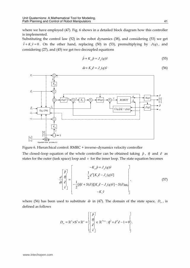
where we have employed (47). Fig. 6 shows in a detailed block diagram how this controller is implemented. Substituting the control law (52) in the robot dynamics (38), and considering (53) we get
0vv K v+ =$# # . On the other hand, replacing (50) in (53), premultiplying by ( )J q , and
considering (27), and (45) we get two decoupled equations
Unit Quaternions: A Mathematical Tool for Modeling, Path Planning and Control of Robot Manipulators
43
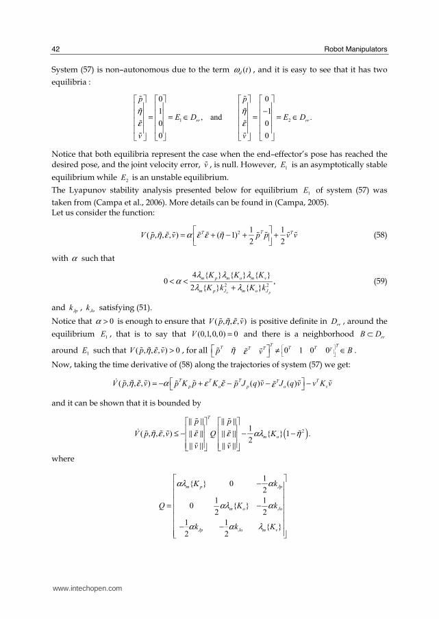
If α satisfies condition (59), then Q is positive definite matrix and ( )V p vη ε, , ,$ # ## # is negative
definite function in rrD , around 1E , that is, (0 1 0 0) 0V , , , =$ and there is a neighborhood
rrB D⊂ around 1E such that ( ) 0η ε, , , <$ # ## #V p v , for all 0 1 0 0TT T TT T T Bp vη ε ⎡ ⎤⎢ ⎥⎣ ⎦⎡ ⎤ ≠ ∈⎣ ⎦## # # .
Thus, according to classical Lyapunov theory (see e.g. (Khalil, 2002)), we can conclude that
the equilibrium 1E is asymptotically stable in rrD . This implies that, starting from an initial
condition near 1E in rrD , the control objective (48) is fulfilled.
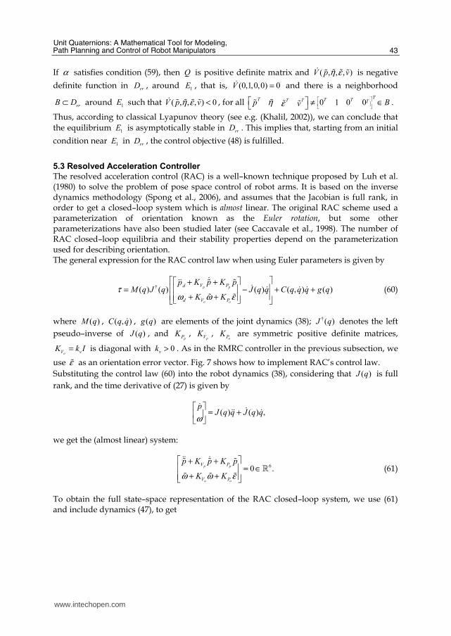
5.3 Resolved Acceleration Controller
The resolved acceleration control (RAC) is a well–known technique proposed by Luh et al. (1980) to solve the problem of pose space control of robot arms. It is based on the inverse dynamics methodology (Spong et al., 2006), and assumes that the Jacobian is full rank, in order to get a closed–loop system which is almost linear. The original RAC scheme used a parameterization of orientation known as the Euler rotation, but some other parameterizations have also been studied later (see Caccavale et al., 1998). The number of RAC closed–loop equilibria and their stability properties depend on the parameterization used for describing orientation. The general expression for the RAC control law when using Euler parameters is given by
where Mdω stands for the supremum of the norm dω .
Let us notice that the position part of system is a second–order linear system, and it is easily proved that this part, considering (63), is asymptotically stable (see, e.g., the proof of the computed–torque controller in (Kelly et al., 2005)). Regarding the orientation part, it should be noticed that
2
1
21( ) ( 1)
{ }2o
T
o
m P
VK
βε εη ε ω η
β λω ω−
−⎡ ⎤⎡ ⎤ ⎡ ⎤, , ≥ − + .⎢ ⎥⎢ ⎥ ⎢ ⎥−⎣ ⎦ ⎣ ⎦⎣ ⎦
# #E E E E# # # ## #E E E E
Thus, given (64), we have that ( )oV η ε ω, ,# # # is a positive definite function in 3 3S ×{ , around
1E , that is to say that (1 0 0) 0oV , , = , and there is a neighborhood 3 3S raB D⊂ × ⊂{ , around
1E , such that ( ) 0oV η ε ω, , ># # # , for all 1 0 0T T
T T T T Bη ε ω ⎡ ⎤⎢ ⎥⎣ ⎦⎡ ⎤ ≠ ∈⎣ ⎦# # # .
The time derivative of ( )oV η ε ω, ,# # # along the trajectories of system (62) results in
1 1( ) ( )
2o o o o
T T T
o P P V V dK K K I K SV η ε ω βε ε ω βη ω βε ω ω−⎡ ⎤ ⎡ ⎤, , = − − − − + ,⎢ ⎥ ⎣ ⎦⎣ ⎦$ # # # # # # # # # #
where properties (4) to (7) on ( )S ε# have been evoked. Hence, we have
( )21 1( ) { } 1
2 2 o
T
o m PQ KVε ε
η ε ω βλ ηω ω
⎡ ⎤ ⎡ ⎤, , ≤ − − − ,⎢ ⎥ ⎢ ⎥⎣ ⎦ ⎣ ⎦
# #E E E E$ # # # ## #E E E E
www.intechopen.com
Robot Manipulators
46
where
M
1
M
{ }
2 { }
o
o
dm P v
dv v m P
K kQ
k k K
βλ β ω
β λ βω−
⎡ ⎤⎡ ⎤− +⎣ ⎦⎢ ⎥= ,⎢ ⎥⎡ ⎤− + −⎣ ⎦⎣ ⎦
the property ( )S x x= has ben considered, and the fact ( )2 21ε η= − was employed to
get the last term.
A condition for ( )oV η ε ω, ,$ # # # to be negative definite in 3 3S R× is that 0Q > , which is true if β
satisfies (5). Thus, ( )oV η ε ω, ,$ # # # is negative definite in 3 3S R× , around 1E , that is to say that
(1 0 0) 0oV , , =$ , and there is a neighborhood 3 3S raB D⊂ × ⊂R , around 1E , such that
( ) 0oV η ε ω, , <$ # # # , for all 1 0 0T T
T T T T Bη ε ω ⎡ ⎤⎢ ⎥⎣ ⎦⎡ ⎤ ≠ ∈⎣ ⎦# # # .
Thus, we can conclude that the equilibrium 1E is asymptotically stable in raD . This implies
that, starting from an initial condition near 1E in raD , the control objective (48) is fulfilled.
6. Conclusion
Among the different parameterizations of the orientation manifold, Euler parameters are of interest because they are unit quaternions, and form a Lie group. This chapter was intended to recall some of the properties of the quaternion algebra, and to show the usage of Euler parameters for modeling, path planning and control of robot manipulators. For many years, the Denavit–Hartenberg parameters have been employed for obtaining the direct kinematic model of robotic mechanisms. Instead of using homogeneous matrices for handling the D-H parameters, we proposed an algorithm that uses the quaternion multiplication as basis, thus being computationally more efficient than matrix multiplication. In addition, we sketched a general methodology for obtaining the dynamic model of serial manipulators when Euler parameters are employed. The so–called spherical linear interpolation (or slerp) is a method for interpolating curves in the orientation manifold. We reviewed such an algorithm, and proposed its application for motion planning in robotics. Finally, we studied the stability of two task space controllers that employ unit quaternions as state variables; such analysis allows us to conclude that both controllers are suitable for motion control tasks in pose space. As a conclusion, even though Euler parameters are still not very known, it is our believe that they constitute a useful tool, not only in the robotics field, but wherever the description of objects in 3-D space is required. More research should be done in these topics.
7. Acknowledgement
This work was partially supported by DGEST and CONACYT (grant 60230), Mexico.
8. References
Aicardi, M.; Caiti, A.; Cannata, G. & Casalino, G. (1995). Stability and robustness analysis of a two layered hierarchical architecture for the closed loop control of robots in the
www.intechopen.com
Unit Quaternions: A Mathematical Tool for Modeling, Path Planning and Control of Robot Manipulators
47
operational space, Proceedings of the IEEE International Conference on Robotics and Automation, pp. 2771–2778, Nagoya, Japan, May 1995.
Barrientos, A.; Peñín, L. F.; Balaguer, C. & Aracil, R. (1997). Fundamentos de Robótica, McGraw-Hill, Madrid.
Caccavale, F.; Natale, C.; Siciliano, B. & Villani, L. (1998) Resolved–acceleration control of robot manipulators: A critical review with experiments. Robotica, Vol. 16, pp. 565–573.
Caccavale, F.; Siciliano, B. & Villani, L. (1999). The role of Euler parameters in robot control, Asian Journal of Control, Vol. 1, pp. 25–34.
Campa, R. (2005). Control de Robots Manipuladores en Espacio de Tarea. Doctoral thesis (in Spanish), CICESE Research Center, Ensenada, Mexico, March 2005.
Campa, R. & de la Torre, H. (2006). On the representations of orientation for pose control tasks in robotics. Proceedings of the VIII Mexican Congress on Robotics Mexico, D.F., October 2006.
Campa, R.; Camarillo, K. & Arias, L. (2006). Kinematic modeling and control of robot manipulators via unit quaternions: Application to a spherical wrist. Proceedings of the 45th IEEE Conference on Decision and Control, San Diego, CA, December 2006.
Craig, J. J. (2005) Introduction to Robotics: Mechanics and Control, Pearson Prentice–Hall, USA, 2005.
Dam, E. B.; Koch, M. & Lillholm, M. (1998) Quaternions, Interpolation and Animation. Technical report DIKU-TR-98/5, University of Copenhagen, Denmark.
Denavit, J. & Hartenberg, E. (1955) A kinematic notation for lower–pair mechanisms based on matrices. Journal of Applied Mechanics, Vol. 77, pp. 215–221.
Fjellstad, O. E. (1994). “Control of unmanned underwater vehicles in six degrees of freedom: a quaternion feedback approach”, Dr.ing. thesis, Norwegian Institute of Technology, Norway.
Gallier, J. (2000). Geometric Methods and Applications for Computer Science and Engineering. Springer–Verlag, New York.
Hamilton, W. R. (1844). On a new species of imaginary quantities connected with a theory of quaternions. Proceedings of the Royal Irish Academy. Vol. 2, pp. 424-434. (http://www.maths.tcd.ie/pub/HistMath/People/Hamilton/Quatern1).
Kelly, R. & Moreno–Valenzuela, J. (2005). Manipulator Motion Control in Operational Space Using Joint Velocity Inner Loop, Automatica, Vol. 41, pp. 1423-1432.
Kelly, R.; Santibáñez, V. & Loría, A. (2005) Control of Robot Manipulators in Joint Space, Springer-Verlag, London.
Khalil, H. K. (2002) Nonlinear Systems, Prentice–Hall, New Jersey.. Khatib, O. (1987). A unified approach for motion and force control of robot manipulators:
The operational space formulation. IEEE Journal of Robotics and Automation. Vol. 3, pp. 43–53.
Krause, P. C.; Wasynczuk, O. & Sudhoff S. D. (2002). Analysis of Electric Machinery and Drive Systems. Wiley-Interscience.
Kuipers, J. B. (1999). Quaternions and rotation sequences. Princeton University Press. Princeton, NJ.
Lin, S. K. (1995) Robot control in Cartesian space, In: Progress in Robotics and Intelligent Systems, Zobrit, G. W. & Ho, C. Y. (Ed.), pp. 85–124, Ablex, New Jersey.
www.intechopen.com
Robot Manipulators
48
Lu, Y. J. & Ren G. X. (2006) A symplectic algorithm for dynamics of rigid–body. Applied Mathematics and Dynamics, Vol. 27, No. 1, pp. 51-57.
Luh, J. Y. S., Walker M. W., Paul R. P. C. (1980). Resolved–acceleration control of mechanical manipulators. IEEE Transactions on Automatic Control. Vol. 25, pp. 486–474.
Natale, C. (2003). Interaction Control of Robot Manipulators: Six degrees–of–freedom Tasks, Springer, Germany.
Rooney, J. & Tanev, T. K. (2003). Contortion and formation structures in the mappings between robotic jointspaces and workspaces. Journal of Robotic Systems, Vol. 20, No. 7, pp. 341–353.
Sciavicco, L. & Siciliano, B. (2000). Modelling and Control of Robot Manipulators, Springer–Verlag, London.
Shivarama, R. & Fahrenthold, E. P. (2004) Hamilton’s equation with Euler parameters for rigid body dynamics modeling Journal of Dynamics Systems, Measurement and Control Vol. 126, pp. 124-130.
Shoemake, K. (1985) Animating rotation with quaternion curves, ACM SIGGRAPH Computer Graphics Vol. 19, No. 3, pp. 245-254.
Spong, M. W.; Hutchinson, S. & Vidyasagar, M. (2006) Robot Modeling and Control, John Wiley and Sons, USA, 2006.
Spring, K. W. (1986). Euler parameters and the use of quaternion algebra in the manipulation of finite rotations: A review. Mechanism and Machine Theory, Vol. 21, No. 5, pp. 365-373.
Whitney, D. E. (1969). Resolved motion rate control of manipulators and human prostheses. IEEE Transactions on Man-Machine Systems, Vol. 10, no. 2, pp. 47-53.
Xian, B.; de Queiroz, M. S.; Dawson, D. & Walker, I. (2004). Task–space tracking control of robot manipulators via quaternion feedback. IEEE Transactions on Robotics and Automation. Vol. 20, pp. 160–167.
Yuan, J. S. C. (1988). Closed-loop manipulator control using quaternion feedback. IEEE Journal of Robotics and Automation. Vol. 4, pp. 434–440.
www.intechopen.com
Robot ManipulatorsEdited by Marco Ceccarelli
ISBN 978-953-7619-06-0Hard cover, 546 pagesPublisher InTechPublished online 01, September, 2008Published in print edition September, 2008
InTech ChinaUnit 405, Office Block, Hotel Equatorial Shanghai No.65, Yan An Road (West), Shanghai, 200040, China
Phone: +86-21-62489820 Fax: +86-21-62489821
In this book we have grouped contributions in 28 chapters from several authors all around the world on theseveral aspects and challenges of research and applications of robots with the aim to show the recentadvances and problems that still need to be considered for future improvements of robot success in worldwideframes. Each chapter addresses a specific area of modeling, design, and application of robots but with an eyeto give an integrated view of what make a robot a unique modern system for many different uses and futurepotential applications. Main attention has been focused on design issues as thought challenging for improvingcapabilities and further possibilities of robots for new and old applications, as seen from today technologiesand research programs. Thus, great attention has been addressed to control aspects that are stronglyevolving also as function of the improvements in robot modeling, sensors, servo-power systems, andinformatics. But even other aspects are considered as of fundamental challenge both in design and use ofrobots with improved performance and capabilities, like for example kinematic design, dynamics, visionintegration.
How to referenceIn order to correctly reference this scholarly work, feel free to copy and paste the following:
Ricardo Campa and Karla Camarillo (2008). Unit Quaternions: A Mathematical Tool for Modeling, PathPlanning and Control of Robot Manipulators, Robot Manipulators, Marco Ceccarelli (Ed.), ISBN: 978-953-7619-06-0, InTech, Available from:http://www.intechopen.com/books/robot_manipulators/unit_quaternions__a_mathematical_tool_for_modeling__path_planning_and_control_of_robot_manipulators


![Quadratic Split Quaternion Polynomials: …...been done for quaternions in [6] and for split quaternions in [2]. Results for generalized quaternions, including split quaternions, can](https://static.documents.pub/doc/80x56/5ea3ed9b0e257f05c666f8d7/quadratic-split-quaternion-polynomials-been-done-for-quaternions-in-6-and.jpg)


