TKK Dissertations 169 Espoo 2009 UNIT-WAVE RESPONSE-BASED MODELING OF ELECTROMECHANICAL NOISE AND VIBRATION OF ELECTRICAL MACHINES Doctoral Dissertation Helsinki University of Technology Faculty of Electronics, Communications and Automation Department of Electrical Engineering Janne Roivainen
Transcript
TKK Dissertations 169Espoo 2009
UNIT-WAVE RESPONSE-BASED MODELING OF ELECTROMECHANICAL NOISE AND VIBRATION OF ELECTRICAL MACHINESDoctoral Dissertation
Helsinki University of TechnologyFaculty of Electronics, Communications and AutomationDepartment of Electrical Engineering
Janne Roivainen
TKK Dissertations 169Espoo 2009
UNIT-WAVE RESPONSE-BASED MODELING OF ELECTROMECHANICAL NOISE AND VIBRATION OF ELECTRICAL MACHINESDoctoral Dissertation
Janne Roivainen
Dissertation for the degree of Doctor of Science in Technology to be presented with due permission of the Faculty of Electronics, Communications and Automation for public examination and debate in Auditorium S4 at Helsinki University of Technology (Espoo, Finland) on the 26th of June, 2009, at 12 noon.
Helsinki University of TechnologyFaculty of Electronics, Communications and AutomationDepartment of Electrical Engineering
Teknillinen korkeakouluElektroniikan, tietoliikenteen ja automaation tiedekuntaSähkötekniikan laitos
Distribution:Helsinki University of TechnologyFaculty of Electronics, Communications and AutomationDepartment of Electrical EngineeringP.O. Box 3000FI - 02015 TKKFINLANDURL: http://sahkotekniikka.tkk.fi/Tel. +358-9-4511Fax +358-9-451 2991E-mail: [email protected]
Monograph Article dissertation (summary + original articles)
Faculty Faculty of Electronics, Communications, and Automation
Department Department of Electrical Engineering
Field of research Electrical machines
Opponent(s) Professor Seamus Garvey, University of Nottingham, UK
Supervisor Professor Antero Arkkio
Instructor Timo Holopainen, D.Sc. (Tech.)
Abstract The primary aim of the thesis is to develop a method for the rapid electromechanical sound power calculation of electrical machines to be used in industry. The core idea is that the numerical simulation of sound radiation is carried out only once. Then, a number of characterizing curves, known as unit-wave responses, are extracted from the results and stored. Finally, the unit-wave responses, together with the magnetic excitation force waves, are used for fast sound power estimation. An experimental method for the determination of unit-wave responses is also developed, which serves especially the process of model verification. The secondary aim is to study the items crucial for the modeling of the sound radiation of electrical machines, such as the effect of tangential force waves on the vibration response, the correlation of force waves in the case of a DTC converter supply, the effect of impregnation on the material properties of the stator core, and the feasibility of the approximate methods for sound power calculation. The most important results of the work done in the thesis include the following: 1) the unit-wave-based sound power calculation performs well, provided that force waves with different wave numbers are weakly correlated, which was verified for the case of a machine supplied by a DTC converter; 2) tangential force waves may have a remarkable effect on the response, which is observed as either an increased or decreased response level, depending on the phase difference of the radial and tangential force waves; 3) the VPI impregnation affects the structural material properties of the stator core considerably, which manifests itself as increased stiffness and decreased damping of the stator core, and 4) the high-frequency boundary element method seems appropriate for the fast and approximate sound power calculation of electrical machinery.
Tiedekunta Elektroniikan, tietoliikenteen ja automaation tiedekunta
Laitos Sähkötekniikan laitos
Tutkimusala Sähkömekaniikka
Vastaväittäjä(t) Prof. Seamus Garvey, University of Nottingham, Englanti
Työn valvoja Prof. Antero Arkkio
Työn ohjaaja TkT Timo Holopainen
Tiivistelmä Työn päätavoitteena on kehittää teollisuuden tarpeisiin soveltuva magneettisen äänitehon laskentamenetelmä. Perusajatuksena on suorittaa varsinainen numeerinen mallinnus vain kerran ja siten, että tuloksista on muodostettavissa konerakenteen akustisia ominaisuuksia kuvaavat yksikköaaltovasteet. Tallennettujen yksikköaaltovasteiden avulla ääniteho voidaan laskea mielivaltaiselle magneettisten voima-aaltojen yhdistelmälle. Työssä esitellään myös menetelmä yksikköaaltovasteiden mittaamiseksi. Mitattujen yksikköaaltovasteiden avulla voidaan selvittää vastaavan matemaattisen mallin oikeellisuus. Työn toisena tavoitteena on tutkia ja ymmärtää sähkökoneen magneettisen äänen laskentaan liittyviä ilmiöitä, kuten tangentiaalivoima-aaltojen vaikutus laskettuihin värähtelyvasteisiin, DTC-taajuusmuuttajalla syötetyn koneen eri aaltolukuisten voima-aaltojen välinen tilastollinen korrelaatio, tyhjökyllästyksen vaikutus staattoripaketin rakennedynaamisiin ominaisuuksiin sekä akustisten likimääräismenetelmien soveltuvuus sähkökoneen äänitehon laskentaan. Työn tuloksena havaittiin seuraavaa: 1) yksikköaaltovasteisiin perustuva äänitehon laskenta on riittävän tarkka, mikäli eri aaltolukuisten voima-aaltojen korrelaatio on heikko, mikä työssä on osoitettukin DTC-taajuusmuuttajasyöttöisen sähkökoneen tapauksessa 2) tangentiaalisten voima-aaltojen vaikutus värähtelyvasteeseen voi olla merkittävä, mikä ilmenee joko vasteen suurenemisena tai pienenemisenä radiaalisen sekä tangentiaalisen voima-aallon vaihe-erosta riippuen 3) tyhjökyllästys jäykistää staattoripakettia sekä pienentää sen häviökerrointa 4) suurtaajuusreunaelementtimenetelmä soveltuu sähkökoneiden äänitehon likimääräislaskentaan hyvin.
No, I won’t go, I will never leave this place Since I feed on that sunshine on your face
And I believe you’ll never tear my soul apart I want to be close to your heart
8
Preface This thesis is the outcome of the research work in the field of vibro-acoustics of rotating electrical machines, carried out at ABB Oy, Machines, Helsinki, Finland during the last decade. Although not comprehensive, this work reports the most important issues discovered by the author during his assignment in ABB. The research work was carried out mainly at ABB Oy, Machines and at several customer locations around the world. The writing of this thesis took place in Helsinki University of Technology (HUT), Faculty of Electronics, Communication and Automation, Laboratory of Electromechanics. Because it is a known truth that a person cannot achieve anything remarkable without the support from the other people, I would like to credit all the people involved with the success of the thesis. I would like to express my gratitude to Emeritus Professor Tapani Jokinen, who encouraged me to embark the post-graduate studies, to my supervising team: Professor Antero Arkkio, Dr. Timo Holopainen/ABB and Mr. Jari Pekola/ABB, and to the head of the laboratory, Professor Asko Niemenmaa. The following people at Technical Research Centre of Finland (VTT) and at HUT have supported me in the form of technical discussion, instruction, and text reviewing over the years and should be acknowledged: Dr. Anouar Belahcen/HUT, Mr. Kari Kantola/HUT, Mr. Paul Klinge/VTT, Mr. Jukka Tanttari/VTT, and Dr. Seppo Uosukainen/VTT. I am very grateful to Mr. Jukka Järvinen/ABB, Mr. Antti Mäkinen/ABB, Tommi Ryyppö/ABB, and Mr. Kari Saarinen/VTT for their work in the field of numerical modeling in this thesis. I would like to thank Mr. Simon Gill at Ruth Vilmi Online Education Ltd for the excellent language checking. The support of ABB Oy, Machines and the financial support of Academy of Finland (Suomen Akatemia) are deeply and gratefully acknowledged. Finally, I thank my mate Arja, my father Osmo, and my sisters Aino and Päivi for being there and especially my mother Lea, who has given me care and support throughout the years. Tuusula, May 2009 Janne Roivainen
9
Contents Abstract 3 Tiivistelmä 5 Preface 8 Contents 9 List of abbreviations 12 List of symbols 13 1 Introduction 17 1.1 Audible noise of rotating electrical machines 17 1.1.1 Noise of magnetic origin 19 1.2 Overview of electromagnetic noise calculation methods 23 1.2.1 Calculation of magnetic forces 25 1.2.2 Calculation of structural vibration 26 1.2.3 Calculation of sound radiation 29 1.3 Aim of the work 32 1.4 Scientific contribution 32 1.5 Outline of the thesis 33 1.6 Literature review of vibro-acoustical research on rotating electrical machines 34 1.6.1 General publications 34 1.6.2 Magnetic forces 35 1.6.3 Structural dynamics of machine structures 35 1.6.4 Material properties of machine structures 37 1.6.5 Sound radiation from electrical machines 37 1.6.6 Effect of frequency converter supply on noise 38 1.6.7 Electromagnetic-vibroacoustical analysis 39 2 Unit-wave response 41 2.1 Introduction 41 2.2 Unit-wave response and frequency response function 42 2.3 Calculation of unit-wave response 44 2.4 Noise and vibration estimation with unit-wave response 45 2.4.1 Direct response 46 2.4.2 Squared response 46 2.4.3 Squared response for weak force wave correlation 47 2.5 Measuring unit-wave response 48
10
3 Magnetic forces 51 3.1 Overview of force calculation method 51 3.1.1 Magnetic field equations 51 3.1.2 Tooth force calculation with Maxwell stress tensor 54 3.1.3 Post-processing of tooth forces 57 3.2 Effect of tangential forces on yoke-bending excitation 61 3.2.1 Types of tangential excitation 61 3.2.2 Combined effect of tangential and radial tooth forces 62 3.3 Effect of DTC converter supply on magnetic forces 64 3.4 Statistical dependence of force waves 69 3.4.1 Background 69 3.4.2 Description of the measurements and force calculation 69 3.4.3 Results and discussion 73 4 Structural dynamics of an electrical machine 77 4.1 Forced structural response: modal superposition 77 4.1.1 Introduction 77 4.1.2 Free response analysis of a damped structure 78 4.1.3 Forced response analysis 79 4.2 Stator material parameters 81 4.2.1 Modeling the stator as a thick orthotropic cylinder with free ends 82 4.2.2 Experimental estimation of natural frequencies and mode shapes 86 4.2.3 Fitting the thick cylinder model to the experimental data 92 4.2.4 Fitting the 3-D solid FEM model to the experimental data 97 4.2.5 Discussion 101 4.3 Effect of tangential forces on stator-yoke vibration response: a simulation study 102 4.3.1 Description of the FE models used in the simulation 102 4.3.2 Total radial bending force 104 4.3.3 Numerical simulations and results 107 4.3.4 Discussion 116 5 Sound power calculation using unit-wave responses 119 5.1 Sound power calculation methods 119 5.1.1 Introduction 119 5.1.2 Boundary element method 119 5.1.3 High-frequency boundary element method 123 5.1.4 Plate approximation method 124 5.1.5 Basic method 126 5.2 Comparison of sound power calculation methods 126 5.2.1 Introduction 126 5.2.2 Description of the numerical model 127 5.2.3 Calculation procedures 129 5.2.4 Comparison of results and discussion 132 5.3 Observations on the unit-wave response-based sound power calculation 135 5.3.1 Introduction 135 5.3.2 Validity of the unit-wave response-based sound power calculation 136
11
5.3.3 Effect of tangential force waves and modal filtering on the calculated sound power 140 5.4 Discussion 142 6 Experimental determination of unit-wave response 145 6.1 Introduction 145 6.2 Description of the measurement method 146 6.2.1 Pre-processing of the response signals 146 6.2.2 Pre-processing of the excitation forces 148 6.2.3 Generation of unit-wave response curves 150 6.3 Effect of sweep rate on the accuracy of the results 153 6.3.1 Introduction 153 6.3.2 Effect of sweep rate on measurement results 154 6.4 Case study: the unit-wave response of a synchronous motor 155 6.4.1 Introduction 155 6.4.2 Description of the measurements 155 6.4.3 Description of the numerical simulations 158 6.4.4 Results and discussion 160 6.5 Discussion 162 7 Summary and Discussion 163 7.1 Summary 163 7.2 Significance of the research 165 7.3 Open issues and future work 167 References 169 A Study on the errors related to the build-up of structural resonance 179 A.1 Numerical study of structural eigenmode build-up 179 A.2 Errors related to the build-up of an eigenmode 182 A.3 Discussion 184
12
List of abbreviations 1-D One-dimensional 2-D Two-dimensional 3-D Three-dimensional ABB Asea Brown Boveri AC Alternating current BEM Boundary element method CHIEF Combined Kirchhoff-Helmholtz integral-equation formulation DC Direct current DTC Direct torque control FCSMEK Finite element program for computation of magnetic fields FEM Finite element method HFBEM High-frequency boundary element method RMS Root mean square SEA Statistical energy analysis RPM Revolutions per minute UWR Unit-wave response VPI Vaporized pressure impregnation
13
List of symbols A magnetic vector potential, surface area, coefficient matrix a general geometric dimension B magnetic flux density b slot pitch, coefficient column vector C viscous damping coefficient matrix, integration path, elasticity matrix c speed of sound, viscous damping coefficient, Kirchhoff-Helmholtz coefficient D dynamic stiffness matrix, electric flux density, differential operator, diameter E expected value operator, electric field strength, Young’s modulus F force, force spectrum f frequency, frequency span, force, force density G autospectrum, gain factor, shear modulus, free space Green’s function g autospectrum H magnetic field strength, hysteretic or structural damping matrix h height, thickness, modal damping factor matrix I identity matrix i index J current density j imaginary unit, index K stiffness matrix, integer k acoustic wave number, index, coefficient, modal stiffness matrix L length, decibel level, differential operator l length M mass matrix, integer m mass, index, modal mass matrix N integer, total number of nodes, number of rows, number of turns in winding n integer, normal vector P power, Cartesian position vector p pole-pair number, pressure or traction Q slot number, generalized force q generalized coordinate, volume velocity R radius, radiation resistance matrix r wave number, radial coordinate, Cartesian position vector S surface or boundary integration area, surface area, sweep rate T time span, window length, torque t time U RMS value of voltage u unit vector, voltage, displacement, x-component of displacement V integration volume, volume v velocity W unit-wave response matrix, time window, width w z-component of displacement, width x free variable, displacement y general response Z radiation impedance matrix
14
z specific acoustic impedance � angle, phase angle � slot pitch angle � Kronecker’s delta, Dirac’s delta function � electric permittivity, normalized random error, mechanical strain φ electric scalar potential, phase angle � square root of coherence function, phase difference � loss factor for hysteretic or structural damping � angular coordinate of cylindrical coordinate system � surface pressure distribution complex angular frequency, eigenvalue magnetic permeability � magnetic reluctivity, Poisson number θ phase difference � mass density, charge density electrical conductivity, acoustic radiation efficiency, mechanical stress � Maxwell stress tensor υ surface normal velocity distribution � angular frequency � viscous damping ratio � difference, frequency bin count, resolution � mass normalized eigenvector Λ eigenvalue matrix Π weighted average normalizing function Ψ eigenvector, beam function Subscripts 0 in vacuum or air a acoustic domain b total radial bending bar rotor bar C converter harmonics c core calc calculated conv total converter dir direction e effective g global F force H harmonic in inner
15
iron iron l local lim limit magn magnetic max maximum meas measured mech mechanical min minimum n normal out outer P plate r radial, wave number, index ϕ circumferential rot rotational rel relative ref reference S sinusoidal, surface, stator T tooth tooth the bottom of a tooth t tangential Y yoke W power, wave Wtot total power Wmagn magnetic power w winding Superscripts g global H Hermitian transpose l local r radial T transpose t tangential * complex conjugate Special notation X Fourier transform (column-wise) or complex matrix
X 2-D Fourier transform of matrix X
16
Notes on font types Vectors and vector fields are typed in bold italics, for example A. Matrices, column vectors, and row vectors are typed in bold, for example K, u, and uT. Trademarks COMSOL Multiphysics is a registered trademark of COMSOL, Inc. DTC is a registered trademark of ABB Oy. MATLAB is a registered trademark of MathWorks, Inc. ME’scopeVES is a registered trademark of Vibrant Technology, Inc. MTS I-DEAS Pro is a registered trademark of the MTS Systems Corporation. NX I-DEAS is a registered trademark of UGS Corp. PULSE is a registered trademark of Brüel & Kjær. SYSNOISE is a registered trademark of LMS Numerical Technologies nv.
17
1 Introduction The demands on modern electrical machines are continuously increasing. Electrical motors are more frequently used in variable-speed drives and thus their operation at resonant speeds has become a critical aspect, together with the increased audible noise and vibration. Simultaneously, the machines should be lighter, noiseless, and more reliable and user-friendly. During recent years, the electrical machine markets have shown a growing interest in high-frequency vibration and noise issues. High frequency in this context means a frequency range from 300 to 8000 Hz. In particular, the process industry and shipyards specify limits for airborne and structure-borne noise for their applications. This poses a challenge for electrical machinery manufacturers in the form of demanding vibration and noise performance characteristics. This fact has to be taken into account in the electrical machine design process. An electrical machine converts mechanical energy to electrical energy, or vice versa. The magnetic field in the air gap of the machine generates the tangential forces required for the torque production. In addition, the field produces other force components that interact with the machine structure and create unwanted vibration and noise. Furthermore, the use of a frequency converter supply creates additional components in the magnetic forces and thus increases the acoustic noise level remarkably. The increase in the A-weighted sound power level can be as high as 15 dB (Belmans & Hameyer 1998). The simulation of the electromagnetic sound power emission of an electrical machine is a three-stage process. First, the magnetic force waves in the air gap are calculated. Then a structure-dynamical model of the electrical machine is created. At this stage, the structural response, usually the vibration velocity, is calculated for the magnetic excitation forces given. Finally, the radiated sound power is calculated. The sound power simulation process that has been described is numerically heavy and time-consuming and thus cannot be considered as an everyday or practical approach to electrical machine design. Furthermore, there is no commercial simulation software available for this specific task. As a result, a new approach is required in order to carry out electromagnetic sound power calculation in a realistic time frame and with realistic effort. In this thesis, a simplified methodology for electromagnetic sound power estimation based on unit-wave responses is presented, studied, and discussed.
1.1 Audible noise of rotating electrical machines The total sound power emission from an electrical machine can be considered as a combination of three uncorrelated noise sources acting together (Timár 1989). These sources are magnetic, cooling, and mechanical or rotational noise sources. An acoustical block model for an electrical machine is presented in Figure 1.1. Magnetic noise is due to the temporal and spatial variations of the magnetic force distribution in the air gap.
18
The operation of the cooling fan creates the bulk of the cooling noise. Rotational noise is generated when: 1) an unsmooth body (rotor) rotates in a cavity that has obstacles and discontinuities, and 2) the shaft and the bearings interact. The magnitude of each source depends heavily on the machine type. The following list presents the major issues affecting each of the sources in an electrical machine: Magnetic noise Pmagn
• shaft load • voltage, current, frequency, and supply type • winding parameters • slot geometry • saturation, eccentricity, etc.
Cooling noise Pcool
• fan type: axial, radial, or mixed flow • rotational speed and fan diameter • airflow velocity • cooling method; closed vs. open, water vs. air
Mechanical or rotational noise Prot
• type of cooling: closed or open • type of bearings • speed
CO O LING M EDI UM FLO W
CO O LING FAN
= airborne = structure-borne A rrows:
SO UR CE (ACTIV E )
B LO CKS : RO TO R-
BE AR ING I NTERA CTIO N
RO TO R RO TA TI ON
S TATO R CO RE
RO TO R & SHA FT
MA G NETI C S TRES S
S TATO R FRA ME
A SS EM BLY FOU ND.
S O UND RA DIA TIO N
PA TH & RES PO NS E (P AS SIV E ) SO UND
R ADI ATIO N SO UND
RADI ATIO N S OUN D
RAD IATIO N S O UND
RA DIA TIO N
S O UND RA DIA TIO N
S O UND RA DIA TIO N
CO O LING S TRUCTURE
CO O LING FA N
BE A RING SHI EL DS
Figure 1.1: Acoustical block model of an electrical machine.
19
The total sound power level LWtot of an electrical machine in decibels can be expressed as
magn cool rotWtot 10
ref
10 log
P P PL
P
+ +� �= � �
� � (1.1)
Here Pref = 1 pW is the reference sound power. Equation 1.1 shows that the total sound power level of an electrical machine is the result of all of the sources. The equation is useful in considering the reduction of the total sound power of an electrical machine. The reduction measures should first be applied to the most dominant source. The following examples clarify this concept:
• For a 2-pole directly-cooled squirrel-cage induction machine, the cooling noise produces 99% of the total sound power, which means that neither the loading nor the converter supply will increase the total sound power level of the machine.
• For an 8-pole totally-closed machine with water cooling, the magnetic noise dominates the total noise output heavily and thus the loading and/or the converter supply will increase the sound power level significantly.
• With a sinusoidal supply, loading the machine can increase the magnetic sound output significantly but with a frequency converter supply, the increase of the noise output is usually much smaller (Wang et al. 2002).
Finally, if the question of how much a certain noise reduction measure affects the total sound power level of the machine is to be answered, one has to know the sound power levels of each of the three sources. If, for example, one faces a situation where the magnetic noise equals the cooling noise, attention should be paid to both of the noise sources in order to achieve satisfactory noise reduction results. If only one of the sources is cancelled out, a maximum reduction of only 3 dB is to be expected. 1.1.1 Noise of magnetic origin A magnetic field in the air gap of an electrical machine is needed to produce the desired torque. The main quantity for the magnetic field is the flux density. A simulated flux density distribution of a small squirrel-cage induction motor is shown in Figure 1.2. In an ideal electrical machine, there exists only the so-called fundamental flux density distribution or fundamental wave BS1 with a frequency equal to the supply frequency ωS1 and the wave number r is equal to the machine pole-pair number p. However, since a real electrical machine has slots and distributed windings, is eccentric, and is magnetically saturated to some extent, the flux density is added with undesired harmonics. As a result, the total flux density distribution in the air gap becomes a sum of rotating flux density waves with various frequencies ωSi and wave numbers ri (Heller & Hamata 1977):
20
( ) ( )S1 S1 S Sj jS S1 S
2...
( , ) Re e e i i ip t r ti
i
t ϕ ω α ϕ ω αϕ − + − +
=
� �= + � �
B B B (1.2)
where BS is the flux density distribution caused by sinusoidal supply, � is the phase angle, and � is the cylindrical coordinate.
Figure 1.2: Simulated flux density distribution of a 15-kW four-pole squirrel-cage induction motor in no-load condition. It should be noted that the flux density distribution expression in Equation 1.2 has a radial and a tangential component. In other words, flux density is a vector field. The harmonics (i �2) create extra losses and sometimes vibration and noise. The harmonic content of the flux density is further increased by introducing a frequency converter supply, which makes the situation even worse. Since the distorted supply voltage contains high-frequency components, each creates a flux density distribution with a wave number equal to the machine pole-pair number but with a frequency different from the supply fundamental. The supply voltage distortion does not create any flux density waves at the new wave numbers; it only adds flux density waves with different frequencies. In this case, Equation 1.2 has to be rewritten in the form
( )C Cjconv S C S C
1...
( , ) ( , ) ( , ) ( , ) Re e k k kr tk
k
t t t t ϕ ω αϕ ϕ ϕ ϕ − +
=
� �= + = + � � B B B B B (1.3)
where Bconv is the flux density distribution caused by the frequency converter supply and BC is the flux density harmonics caused by the frequency converter supply. Thus, in addition to the creation of torque, a large number of radial and tangential forces are also generated as a side product. The reluctance force density dF in cylindrical coordinates acting on the stator surface can be calculated from the following equation based on the Maxwell stress tensor (Belahcen & Arkkio 2000):
21
( ) ( )2 2
0
1d d
� 2 r r r
LB B B B rϕ ϕ ϕ ϕ� �= − + � �
F u u (1.4)
where L is the axial length of the air gap, r is the radius of the air gap, �0 is the permeability of the vacuum (air), Br is the radial flux density, B� is the tangential or circumferential flux density, and ur, u� are radial and circumferential unit vectors. Usually, the integration of Equation 1.4 is carried out stator tooth-wise. The result is a radial and a tangential tooth force, together with the total torque acting on each tooth. This approach can be justified by the fact that the forces are much higher in amplitude in the region of the tip of the tooth than at its root (Belahcen 1999). Numerical magnetic field solvers can use Equation 1.4 directly to calculate the forces acting on the stator teeth. For analytical calculations, Equation 1.4 is simplified because only the radial flux density component is usually calculated using those methods. This principle is justified for unloaded machines to some extent but not for the loaded case, because the tangential flux density usually becomes larger with loading. Nevertheless, this approach simplifies the equations and still shows the main aspects of force generation in rotating electrical machines. If the tangential flux density is set to zero, Equation 1.4 becomes
2
0
d d2�
rr r
BLr ϕ=F u (1.5)
If Equation 1.2 is rewritten in terms of radial fundamental BS1r and harmonics BSHr like
S S1 SH r r rB B B= + (1.6) and by inserting Equation 1.6 into Equation 1.5, one gets
( )2S1 SH
0
d d2�
r rr r
B BLr ϕ
+=F u (1.7)
As the flux density is expressed as a sum of the cosine waves rotating in the air gap, the resulting radial tooth force distribution Fr is also a sum of waves
( ) ,, cos( )r r i i i i
i
F t F r tϕ ϕ ω φ= + + (1.8)
where ri is the wave number of force wave i and �i is the frequency of force wave i in the stator coordinate system. As mentioned, the radial tooth force distribution is in fact a sum of rotating waves with different wave numbers and speeds (frequencies for static observer in stator frame of reference). To illustrate the wave nature of the radial forces, the waves with wave numbers ri = 2, 3, and 6 are shown in Figure 1.3.
22
-0.5
0
0.5-0.4
-0.2
0
0.2
0.4
0
0.2
0.4
0.6
0.8
1
-0.4
-0.2
0
0.2
0.4
0.6-0.5
0
0.50
0.2
0.4
0.6
0.8
1
-0.5
0
0.5-0.5
0
0.5
0
0.2
0.4
0.6
0.8
1
Figure 1.3: Rotating force waves, from left to right ri = 2, 3, and 6. As an example, the radial forces of an induction machine at no-load, supplied from a sinusoidal voltage source, are calculated with an analytical method (Maliti 2000) and the results are shown in Figure 1.4. The figure is informative, as all of the essential features are shown. The y-axis presents the wave numbers of the force waves and, as one can see, there also exist negative wave numbers, which in this case means that they rotate in the opposite direction with respect to the rotor of the machine.
Figure 1.4: Radial tooth force wave number frequency distribution of an induction motor. The color scale is in decibels referenced to 1 N. The rotating force components try to deflect the structure they act on; in other words, they make the machine stator, frame, and foundation vibrate. The level of vibration depends on three factors:
1) The frequency, wave number, and amplitude of the force wave. 2) The existence of any proper or suitable structural mode at the exciting
frequency. 3) The structural damping of the stator, frame, and foundation.
23
The conditions for a high vibration level and thus noise radiation are met if the shape and frequency of the force wave match any of the structural mode shape and natural frequency. In this case, only the damping properties of the structure limit the vibration level. The higher the damping, the lower the vibration levels, and vice versa. In welded steel frame machines, the side plates of the frame are usually the main radiators of magnetic noise. The bearing shields or machine ends rarely radiate remarkable levels of sound power. In some cases, the foundation also radiates sound. It should be noted here that only the surface normal vibration velocity can create sound waves. In-plane vibration cannot generate sound waves since the surrounding air transmits shear stresses poorly. An estimate for the sound power level radiated by a vibrating surface can be calculated from Equation 1.9 (Cremer et al. 1987):
20 n
W 10ref
10log
A c vL
P
σρ� �� �=� �� �� �
(1.9)
where LW is the sound power level, A is the area of the radiator, σ is the radiation efficiency (Cremer et al. 1987), ρ is the density of air, c0 is the speed of sound, and �|vn|2� is the spatially averaged mean-squared normal velocity RMS. Looking at Equation 1.9, it can be observed that the most effective way to reduce the radiated sound is to reduce the normal vibration of the surface. Because the vibration velocity is directly proportional to the radial tooth force amplitude, which in turn is proportional to the square of flux density B, the following holds (Timár & Lai 1994):
( ) ( )4 4Wmagn 10 Wmagn 1010 log or 10 logL B L U� � (1.10)
The symbol U represents the supply voltage. Equation 1.9 simply states that if, for example, the terminal voltage of the machine is reduced by 50%, both the sound power and pressure levels will be reduced by 12 dB. 1.2 Overview of electromagnetic noise calculation
methods In principle, all the activities around electromagnetic noise are somehow linked to the block diagram shown in Figure 1.5. The vibro-acoustical part of the block diagram (mechanical and acoustical) is common to all areas of machinery acoustics. The stator and rotor cores are the only exceptions, since they are made out of steel laminations. The laminated nature of these components sometimes makes the structural analysis difficult because their material parameters are orthotropic (Garvey et al. 1999c; Wang 1998) and depend on manufacturing practices such as the axial pre-stressing of the core before the laminated stacks are joined together (Dias Jr 1999; Watanabe et al. 1983). Variations in temperature pose another challenge as the material properties of the resin used in the impregnation of the windings are known to depend on the temperature
24
(Watanabe et al. 1983). The generation mechanisms of the magnetic forces at the air-iron boundaries and in the iron itself are unique to electrical machines and in order to understand them better, a lot of scientific research and development has been done on the topic over the years. The issues mentioned above make the noise of electrical machines a well-defined research topic in its own right in the field of machinery acoustics.
ELECTRO-MAGNETICPROCESS
MECHANICALPROCESS
ACOUSTICALPROCESSU
pmagn vmech
Lw
Coupling Coupling
Figure 1.5: Electromagnetic noise generation process (Gieras et al. 2006). Generally speaking, one is interested in how much sound power Lw is produced with a given input voltage U to the system in Figure 1.5. The answer can be found by simply measuring the sound power of the system under stationary conditions. If the sound power level is too high, it has to be reduced by modifying the system in some way. One way of reducing the noise output would be to make changes to the system and measure the sound power again, which is the well-known trial-and-error method. The method requires a large number of test runs and it is known not to be an efficient way of controlling noise. More efficient ways include the use of mathematical models to simulate the effect of modifications on the noise output. Mathematical models help in understanding the physical nature of sound power generation. By using either analytical or numerical models to describe the electromagnetic process, one can understand the inter-relations between the input voltage and magnetic stress or pressure pmagn through electromagnetic process parameters such as the slot number or the skewing of the rotor slots. The same holds true for the vibro-acoustical part of the system. The simulations can show how the surface normal velocity vmech is related to pmagn through mechanical process parameters such as plate thicknesses. The simulations of an acoustical process model reveal whether the use of perforated plates on the surface of the machine will reduce the sound power level, for example. It is then the responsibility of the manufacturer of the machine to decide which of the available modifications will be put into practice. The magnetic field and structure of the machine are coupled together. In cases where the rotor deflections are large, the effects of coupling can be observed clearly, which complicates the modeling task. In some cases, the surrounding fluid may couple the structural vibration and fluid loading together, which is known as fluid-structure interaction. In this thesis, however, these coupling effects are ignored.
25
1.2.1 Calculation of magnetic forces As an electrical machine operates, there will be forces and torques acting on its structure. The shaft torque is naturally the one to be maximized and all the other forces and torques are considered as parasitic in nature, i.e., they do not participate in the process of feeding active power to the desired process. Three types of magnetic forces exist in an electrical machine:
1. The reluctance force, which acts on the boundaries of materials with different magnetic properties.
2. The Lorentz force, which acts on currents in the magnetic field. 3. The magnetostrictive force, which acts inside the iron core.
The air gap between the stator and rotor is the region where the reluctance force acts, and the tooth tips especially serve as an interface for the forces to deliver parasitic energy to the structure. The forces depend on the geometry of the slots, the length of the air gap, the winding arrangements, the degree of saturation, etc. The reluctance force is the most important excitation type, since its magnitude is usually the largest when compared with the other two forces. The Lorentz force acts on the windings of the machine, but since the flux density in a slot is small, the force remains quite negligible. Thus, this force type is not included in this thesis. Magnetostriction can play an important role in the excitation of structures (Belahcen 2006; Delaere et al. 2000; Garvey & Glew 1999a; Låftman 1995) but because of its complexity and because this thesis is not about force calculation it is also ignored. Since the reluctance force or stress is a 3-D vector and the air gap is cylindrical, a division into radial, tangential/circumferential, and axial components is reasonable. The radial components are usually the greatest in magnitude and they originate from the magnetic field trying to close the air gap. The magnitudes of the tangential components are usually smaller than those of the radial ones, but the static component (r = 0), which has a non-zero value when integrated around the rotor circumference produces the desired torque. Axial forces are usually negligible. In summary, in order to achieve the desired torque performance, additional radial and circumferential components are also introduced. When the mechanical design of an electrical machine is under consideration, one of the key points of interest is whether the structure can withstand all the forces acting on it. One source of stress is the magnetic forces acting on the machine, and it would be desirable to estimate their magnitudes. Sometimes, even a small magnetic force component, which is harmless to the structure, can be annoying to the user of the machine if it creates acoustic noise or vibration. The force component is dynamic in nature and has a certain spatial distribution around the air gap. The radial and tangential
26
force components are usually responsible for the creation of sound, and thus their properties play a key role in magnetic noise generation. A number of methods are available for calculating the magnetic force in the air gap. Conformal mapping and Fourier wave decomposition, also known as the rotating field theory, are the most traditional methods for force estimation. Their common feature is that they are analytic since they can often express the force distribution in a closed form. The finite element method (FEM) and reluctance networks represent a more modern approach to the estimation of magnetic force or traction and they can be considered to be numerical because of the need for large matrix computation involved in the solution. All the methods mentioned above usually assume 2-D geometry, because the axial phenomena are traditionally considered negligible and since the computation resources needed are huge with 3-D models. In the case of axial variation of eccentricity, such as a tilted rotor, the magnetic force also adopts variation in the axial direction. The advantages of using traditional methods, especially Fourier wave decomposition, are that they keep track of the origins of each component of the magnetic force, are computationally light and fast, and serve educational aspects very well. The drawback of these methods is that they can model only global effects and thus the accuracy of the estimation is somewhat degraded. For example, the saturation of the tooth-tip region is very difficult to model analytically. Analytical methods usually assume that
• The machine is 2-dimensional. • Saturation affects the effective air gap. • The material characteristics of iron parts are assumed to be linear and of zero
reluctance. • The magnetic field consists only of a radial component. • Skin effects and other eddy-current effects are excluded. • The supply is a symmetric three-phase sinusoidal current source.
Numerical methods are more accurate and can handle non-linearity and localized effects such as local saturation, and can operate directly in the time domain without any assumptions of time-harmonicity, but the price that is paid for this is the demand for high computing power and the degradation of physical insight. 1.2.2 Calculation of structural vibration Time-varying forces acting on a structure cause vibration. If the forces are time-harmonic, their amplitudes, spatial distribution, and frequency determine how much vibration is observed. Every structure has an infinite number of natural frequencies and related mode shapes. If the excitation frequency matches one of the natural frequencies of the structure and if the excitation pattern and the mode shape are similar, then even low excitation levels can create large vibration amplitudes. This modal behavior of
27
structures has been of interest to a large number of researchers for the last hundred years. The equations of motion for a continuous elastic structure are partial differential equations, which can be solved for simple geometries such as a rod, beam, membrane, plate, cylinder, sphere, and so forth (Cremer et al. 1987). The trial function has to respect the boundary conditions in order to be a proper solution. For example, the equation of motion for an un-damped thin plate in bending, i.e. only movement in the direction normal to the plate surface, is (Soedel 1993):
2
2
d ( , , )( , , ) ( , , )
d z
w x y tLw x y t m p x y t
t+ = (1.11)
In Equation 1.11, L is a differential operator, w is a displacement in the normal direction (z-direction) of the plate, m is the surface mass density, and pz is the pressure or force density distribution acting on the plate surface. If the forcing term on the right-hand side of Equation 1.11 is set to zero, the equation of motion becomes a free vibration problem in which time-harmonic motion with angular frequency ω is assumed
2( , ) ( , ) 0Lw x y mw x yω− = (1.12) The solutions to Equation 1.12 can exist only at certain values of ω. These values are the natural frequencies or eigenvalues of the system (Newland 1989). Nowadays, there are many ways to analyze structural vibration but the following are perhaps the most used and popular:
1. Analytical methods for simple geometries. 2. Deterministic numerical methods such as FEM. 3. Statistical Energy Analysis (SEA). 4. Hybrid FEM/SEA methods.
The analytical methods are the oldest tools for the vibration analysis of structures. The early vibration analyses of electrical machines (Erdelyi 1955) treated the stator as a ring, for which the natural frequencies were calculated. The design rule was to avoid hitting these frequencies with magnetic excitation. Later on, the stator and frame were treated as a 3-D cylinder (Verma & Girgis 1981a). This approach is still sometimes used (Wang & Lai 2000a) because the analysis becomes simple and fast. The analytical methods are suitable for both the free and forced vibration analysis of the structure. With the rapid development of computers, deterministic numerical methods are almost de facto tools for vibration analyses today. The formulation of the equations of motion into a form suitable for numerical calculation is done through variational calculus. The most popular method is FEM, which is also widely used in electrical machine vibration analysis. Deterministic numerical methods can be applied to almost any kind of problem, i.e., they can be used directly in the time domain for nonlinear problems, they
28
can be used for free and forced response analyses, etc. One drawback of the deterministic numerical vibration analysis methods is that they usually require large computing resources for reasonable solution times. Even though it is an accurate and useful computational method of electrical machine vibration analysis, FEM is suitable only for problems at lower frequencies or for problems which deal with the so-called global behavior of structures. Low frequencies in this context are related to the dimensions of the structure and to the solution wavelength. If the excitations in the problem have energy at higher frequencies, FEM might not be an appropriate tool for solving the problem. The reasons for this are the following (Fahy & Walker 2004):
• At higher frequencies, the local modes are being excited, and these typically have short wavelength characteristics, i.e. the deformation patterns are highly complex and detailed. This leads to a requirement for an extremely fine model mesh. In order to avoid spatial aliasing, the mesh density should be approximately ten node points per wavelength. At some point, it becomes impractical to use FEM for the calculation of modes, for example.
• The other problem is the increase of modal density as a function of frequency. This means that the modes start to overlap each other, leading to significant errors if the damping in the structure is not evenly distributed. Naturally, the high modal density itself causes problems for the storage of results and increases solution times.
• The natural frequencies and mode shapes become more sensitive to structural details as the frequency is increased. This means that the model needs more and more detailed material parameters, joint properties, boundary conditions, etc. Finally, the problem cannot be solved any more, no matter how massive the computing resources available are.
If vibration analysis has to be carried out at high frequencies, one has to give up the requirement of deterministic models. SEA has been widely used to study the high-frequency behavior of structures (Delaere et al. 1999a; Lyon & DeJong 1995; Wang 1998; Wang & Lai 2005). In SEA, the structure is divided into subsystems component-wise, i.e., one side plate of an electrical machine is one subsystem, the stator as a whole is another, and so on. The primary variables are the vibration energies and powers of the subsystems. The SEA has similarities to the diffusion equation in heat problems, i.e., the energy level differences tend to even out. The analysis results are the average quantities in subsystems, such as the averaged squared normal velocity of a plate. There are no node-wise results available such as vibration amplitude and phase. Contrary to FEM, SEA works well at high frequencies but fails at low frequencies. The frequency limit depends heavily on the problem. The most recent method in vibration analysis is the Hybrid FEM/SEA method (Langley et al. 2005; Langley 2007; Shorter & Langley 2005a, b). In this method, the subsystems with low modal density or a long wavelength are modeled with FEM, whereas the subsystems with high modal density or a short wavelength are handled with statistical
29
methods such as SEA. The equations of motion with viscous damping are written as (Fahy & Walker 2004):
2( j )ω ω+ − = =K C M q Dq F (1.13) Equation 1.13 is partitioned in the form
g ggg gl
l lgl llT
� �� � � �=
� � � �� �
D D q FD D q F
(1.14)
In Equation 1.14, the sub- or superscript g refers to a global or long wavelength component and l refers to a local or short wavelength component. D is the dynamic stiffness matrix and q is the vector of generalized coordinates describing the motion of the system. Equation 1.14 is the basis for a simultaneous solution combining FEM with some statistical method. 1.2.3 Calculation of sound radiation A vibrating surface can radiate sound. More specifically, it is the surface-normal vibration that acts as a boundary condition for sound radiation problems. In this thesis, only the radiation into infinite space is dealt with. Thus, no interior problems, scattering, or suchlike are studied or discussed. A time-harmonic acoustic wave in free space that has no sources obeys the Helmholtz equation (Morse & Ingard 1968):
2 2
0
0, c
p k p kω∇ + = = (1.15)
where p is the sound pressure, k is the wave number, ω is the angular frequency, and c0 is the speed of sound in the fluid in question. A normal velocity boundary condition is given as the Neumann condition, the pressure boundary condition is given as the Dirichlet boundary condition, and surface acoustic impedance is specified with the Robin boundary condition (Kirkup 1998). For simple geometries such as an infinite plane, cylinder, sphere, elliptical cylinder, and so on, Equation 1.15 can be solved analytically using specific functions for the given problem geometry. For example, spherical problems are solved through the use of Legendre functions and cylindrical problems with combinations of Bessel functions known as Hankel functions (Williams et al. 1987). Wang and Lai (2001, 2000b) modeled the sound radiation of an induction motor using analytical expressions for a cylindrical sound radiation problem. An earlier work in this area (Ellison & Moore 1968) modeled an electrical machine as a sphere for sound power calculation. The integral form of Equation 1.15 is written as (Herrin et al. 2006):
30
0 n S
j
( )( ) ( ) j ( ) d
e( )
4�
S
kr
G rc P p P v G r p S
n
G rr
ρ ω
−
∂� �= + ∂� �
=
� (1.16)
Figure 1.6: Description of the quantities in Equation 1.16 (Herrin et al. 2006). Equation 1.16 is also known as the Kirchhoff-Helmholtz integral equation for sound radiation (Kirkup 1998). In Equation 1.16, ρ0 is the density of fluid, vn is the surface normal velocity distribution, ps is the surface sound pressure distribution, and G(r) is the free-field Green’s function. The coefficient c(P) is equal to 1 for P in the acoustic domain, and equals 1/2 if P is located on a smooth boundary (Herrin et al. 2006). If both vn and ps are known, the evaluation of Equation 1.16 is straightforward. Usually, only vn is known and ps has to be solved either with some numerical method or, if the problem geometry is simple, with an analytical method. If the boundary S is a flat plate lying on an infinite plane, Equation 1.16 reduces to Rayleigh's second integral (Langley 2007):
0 n( ) 2 j ( )dS
p P v G r Sρ ω= � (1.17)
Equation 1.17 is widely used in approximate methods for sound power calculation (Seybert & Herrin 1999). In the roughest approximations, Equation 1.17 is directly applied to any kind of a vibrating body, thus neglecting the requirement for flatness (Seybert & Herrin 1999). The power of the approximation methods based on the Rayleigh integral is that even if the sound pressure field calculated with Equation 1.17 is not correct, the sound power emission can provide acceptable results, since the sound power is proportional to the surface integral of the squared far-field pressure; it is a known fact that integration smooths information through summing.
Radiating body
31
If the sound radiation resides at high frequencies, Equation 1.16 can be approximated by using the following expression to estimate the sound pressure on the surface S
S 0 0 np c vρ≈ (1.18) Equation 1.18 is inserted into Equation 1.16 and the sound power estimation can be carried out. The method is known as high-frequency BEM (HFBEM), as presented by Herrin et al. (2006). The boundary element method (BEM) is the most widely used numerical method for calculating sound radiation from vibrating bodies (Ciskowski & Brebbia 1991). In BEM, the problem can be infinite, i.e., no outer boundaries for the problem are required. The Sommerfeld radiation condition is automatically fulfilled with BEM. The sound radiation problem can also be solved with finite elements but in this case a control surface is required at some distance from the radiating surface S, since FEM needs a bounded geometry for the definition of the problem. The Sommerfeld radiation condition has to be fulfilled with special types of elements at the control surface (Fahy & Walker 2004). Moreover, FEM requires the whole volume between S and the control surface to be meshed. In BEM, only the radiating surface needs to be meshed (Kirkup 1998). In BEM, the formulation of the problem starts with Equation 1.16, which is then discretized element-wise at the boundary S. The solution procedure has the following steps:
1. Assuming that the normal velocity is given, the unknown sound pressures on a surface S are solved. The procedure is called boundary integral equation solving. Mixed boundary conditions are also possible.
2. Once the boundary pressures are known, the far-field pressures at specified points can be calculated using the discretized version of Equation 1.16. The sound power calculation can also be carried out directly with vn and ps.
BEM is computationally heavy, since the system has to be solved for all frequencies of interest; the system matrices are usually full, unsymmetric (direct method), and complex. Like structural FEM, BEM is not a good tool for high-frequency sound radiation problems because the mesh density will become too high at higher frequencies. BEM is an appropriate method at frequencies at which the acoustic wavelength is of the order of the radiating body. Statistical methods such as SEA can also be used for high-frequency radiation problems. In SEA, Equation 1.9 is exploited directly, since it includes the mean-squared velocity as an input, which is directly available from the SEA results. The radiation efficiency in Equation 1.9 is usually calculated by the use of analytical expressions (Lyon & DeJong 1995; Wang & Lai 2000b)
32
1.3 Aim of the work This thesis serves five purposes. The first aim is to develop a methodology to simulate vibration and sound power emission from electrical machinery using unit-wave responses. The use of unit-wave responses provides the designer of an electrical machine with a much deeper insight into the vibro-acoustical behavior of the system that is being dealt with. The unit-wave response also facilitates a more efficient re-use of the vibro-acoustical simulation models. The unit-wave response can be thought of as the “fingerprint” of the structure of an electrical machine. The second aim is to create a method to determine the unit-wave response experimentally. The goal is to be able to use the existing magnetic configuration of the machine for estimating the unit-wave response. Thus, no special winding arrangement is needed in the measurement process. The third aim concentrates on investigating the phenomenon of reluctance force excitation at the iron-air interface. In particular, the effects of tangential forces on the vibro-acoustical response are studied in depth. An attempt to expand the work of Garvey (1999b) is made. The fourth aim is to study the material properties of a stator of an electrical machine. The knowledge of correct stator material parameters is crucial for the successful simulation of noise. Special attention is paid to the material damping and to the effect of vaporized pressure impregnation (VPI) on the material properties of the stator core. The fifth aim concentrates on studying approximate methods to estimate the sound power emission of electrical machines, especially welded steel-frame machines.
1.4 Scientific contribution The scientific contribution is comprised of the following items: 1. A method for the simple and fast modeling of the vibro-acoustical behavior of
electrical machines. 2. Unit-wave response-based sound power estimation. 3. A method for the experimental determination of the unit-wave response. 4. Error curves for correction of the curve-fit errors involved in speed ramp
measurements. 5. Tangential tooth forces either increase or reduce the vibration of the stator yoke,
depending on the phase difference between the radial and tangential force wave. 6. In the case of a DTC converter supply, the correlation between the force waves with
different wave numbers is weak. 7. A method for the extraction of complex stator material parameters.
33
8. VPI impregnation increases the stiffness and reduces the damping of the stator core. 9. The high-frequency boundary element method is suitable for the approximate
estimation of the sound power of welded steel electrical machines. 1.5 Outline of the thesis This chapter is intended to serve as an introduction to the field of the vibro-acoustics of electrical machinery. This chapter also includes a literature review of the essential work carried out by others. Chapter 2 introduces the concept of unit-wave response. It also presents a procedure for calculating the vibro-acoustical response of an electrical machine, such as the mean-squared normal velocities of the machine surface. Chapter 3 describes the magnetic force calculation method used in this thesis. It also includes a treatise on tangential force coupling with yoke radial bending by the use of analytical formulation. Furthermore, the nature of a DTC converter supply is discussed, since it is very likely that the force waves created by the DTC converter supply are weakly correlated with each other. This simplifies the use of the unit-wave response for response calculation. Chapter 4 describes the calculation method used in the thesis to predict the vibration of the machine structure. The method is known as a modal superposition principle. A study of the effect of tangential forces on the stator vibration is made using numerical simulations. The validity of the analytical formulation presented in Chapter 3 is tested thereby. The complex material properties of the stator are extracted using an experimental modal analysis and thick cylinder model based on the Rayleigh-Ritz method. There is special interest in the effect of VPI impregnation on the material properties of the stator core. The validity of the thick cylinder model is investigated by comparing the calculated results with the results obtained from a full 3-D solid model of the same stator. Chapter 5 concentrates on issues related to the calculation of sound power emission from an electrical machine. The direct formulation of the boundary element method is presented briefly. A review of approximate methods is made and they are tested by comparing the sound power level calculated by commercial BEM to the sound power level obtained with the methods reviewed. A comparison is also made between the sound power level calculated through unit-wave responses and the sound power level obtained directly. Chapter 6 presents a method to determine the unit-wave response experimentally by sweeping the machine speed with a constant flux and at no-load conditions. The errors introduced by the sweep measurements are also studied. Chapter 7 includes the discussion and conclusions based on the results obtained in this thesis.
34
1.6 Literature review of vibro-acoustical research on rotating electrical machines
The electromagnetic noise of electrical machines has perhaps been studied ever since the discovery of the electro-magneto-mechanical energy conversion, which means a time span of more than a century. The subject is also very broad, as discussed in the previous sections, so a division of the previous research into different classes is necessary. The vibro-acoustical research work is classified as follows:
1. General texts, papers, and reviews of machinery noise dealing with all the noise sources in electrical machinery.
2. Calculation of the magnetic forces in the air gap and in iron parts. 3. Investigations of the structural dynamics of electrical machines 4. Estimation of stator material properties, such as Young’s modulus, shear
modulus, Poisson’s number, and damping factors. 5. Modeling of sound radiation from a machine structure. 6. Effect of frequency converter supply on magnetic noise. 7. Full electromagnetic-vibro-acoustical analysis (simulation & measurements).
1.6.1 General publications Ellison and Moore (1968) published a paper in which the noise of electrical machines was discussed and qualitatively analyzed in depth. The paper also has a good bibliography of the research work carried out on the subject before 1968. The well known book by Yang (1981) added more of a quantitative approach to the calculation of the magnetic noise of electrical machines. Yang used the rotating field theory in his work to calculate the magnetic reluctance forces in the air gap and utilized a cylindrical solution of the Helmholtz equation for sound radiation. The book edited by Timár (1989) can be considered as an expanded version of Yang’s book. Timár also introduced the important concepts of random signal analysis, such as the quantity called coherence. It is also crucial in this context to mention the book about noise measurements of electrical machinery by Yang & Ellison (1985). The article by Finley (1991) discusses noise issues in electrical machines and it also contains a list of measures for reducing the noise from an electrical machine. Later on, Finley published articles on general problems with electrical machines, such as starting torque problems, bearings, vibration, temperature issues, and so on. The papers also include short discussions of machinery noise (Finley & Burke 1994; Finley et al. 1999). Vijayraghavan and Krishnan (1999) published a paper with an approach similar to Ellison and Moore (1968) with an updated bibliography. In his review article Nau (2000) also discussed the effect of a frequency converter on the magnetic noise and he also gave a list of measures to be taken in order to reduce noise levels in electrical machinery.
35
The most recent comprehensive work on noise in electrical machines is the book written by Gieras et al. (2006). It discusses the use of analytical and numerical methods in the calculation of magnetic noise in machines. SEA is also introduced in the book. 1.6.2 Magnetic forces A great amount of effort has been put into the calculation of magnetic fields and the reluctance forces they produce in the air gap of an electrical machine, since the reluctance forces are the main origin of magnetic noise. The importance of proper slot combination was understood quite early (Chapman 1922). He listed rules for slot combinations in squirrel-cage motors. Verma and Balan (1994) used the rotating field theory together with the Maxwell stress expression to derive the forces acting on the stator surface, and they also described the multiple armature reaction in an understandable way. Gerling (1994) studied the effect of different formulations of a permeance wave on the calculated radial force in the air gap. Akiyama et al. (1996) studied the use of uneven rotor slot pitch and its effect on radial forces using FEM, and they came up with encouraging results. Belahcen et al. (1999) calculated the forces acting on the stator surface and carried out 2-D FFT from the time-space domain to the wave number-frequency domain. They used time-stepping FEM together with Maxwell stress in their analysis. Belahcen & Arkkio (2000) also compared the principle of virtual work and Maxwell stress in force calculation. In addition, they calculated the forces acting on the stator teeth, thus reducing the amount of data needed to describe the forces. It was also shown that the forces located in the tooth-tip region are much larger than those in other parts of the tooth. As a continuation of the earlier work, Belahcen (2001) published a review paper on the methods used for the calculation of the forces. In his paper, he found that nodal force methods can give better estimates for forces than the Maxwell stress method. Maliti (2000) performed an in-depth analysis of radial force calculation through the use of rotational field theory. He also studied the effect of eccentricity on magnetic noise. Delaere et al. (2003) used 2-D FEM to study the effect of the ferromagnetic slot wedges of the rotor on the stator vibration and noise. They showed that the ferromagnetic wedges reduce the harmonic content in the stator current and thus can bring the magnetic noise levels down. 1.6.3 Structural dynamics of machine structures Verma and Girgis (1981a) modeled the teeth, windings, stator, and frame of an electrical machine using the Rayleigh-Ritz method. The main goal of the work was to predict the natural frequencies and mode shapes of the system. To test their model, they performed extensive experimental modal analyses for eight different machine components and found a reasonable correlation between the calculations and measurements (Verma & Girgis 1981b, c).
36
Watanabe et al. (1983) published a paper in which they studied the properties of medium-sized stators. They looked into the effect of the axial clamping force, teeth, windings, wedges, impregnation, and temperature on the modal properties of stators. They found out that the teeth introduce rotational inertia, the clamping force has a small effect on modes, the wedges and impregnation stiffen the stator, and that the temperature affects the damping more than the elastic properties of the stator. Verma et al. (1987a, b) calculated the eigenproperties of a thick isotropic cylinder with the Rayleigh-Ritz method. They also carried out an experimental modal analysis for a steel cylinder with the same dimensions as the modeled one. The correlation between the measurements and simulation was found to be good. The idea behind the work was to model the stator yoke of an electrical machine as a thick cylinder. Garvey (1988) studied the use of substructuring methods and special element types for analyzing the structural behavior of a large DC machine with 3-D FEM. He also did experiments to extract the material parameters of joints and laminated (stacked) components specific to electrical machines. Garvey & LeFlem (1999b) published an important paper about tangential forces and their effect on the stator vibration response. In the paper, it was shown that the tangential forces acting on the tips of the stator teeth can have an effect on the vibration responses. Furthermore, the method of sweeping a unit amplitude force wave through the frequencies of interest was used. Benbouzid et al. (1993) investigated the structural behavior of a stator with 3-D FEM. They simulated the modal properties of the stator with different configurations similar to those of Watanabe et al. (1983) and the results also showed similar behavior. The only exception was that a 3-D model was used instead of a 2-D model. Chang & Yacamini (1996) simulated the effect of imperfections on the symmetrical behavior of a ring. They also performed an experimental modal analysis on a machine stator frame configuration. The result of the work was that every slot or discontinuity in a cylindrical structure introduces more modes. Wang & Williams (1996) classified the modes of a thick isotropic cylinder both numerically (3-D FEM) and experimentally. They also studied the effect of the dimensions on the eigenproperties of the cylinder. They then continued to study the behavior of a laminated cylinder, resembling a stator (Wang & Williams 1997), and came up with the result that an axial lamination destroys some of the modes existing in a homogeneous cylinder, leaving only the pure radial modes. Colby et al. (1996) used 2-D FEM to calculate the eigenproperties of the stator of a four-phase switched reluctance motor. They also derived a simple equation to calculate the natural frequencies of the stator. The simulation results were verified by experimental results and a good agreement was found. Experimental modal testing is usually carried out with excitation being introduced point-wise, such as shaker or impact hammer excitation. The approach excites almost every mode in the structure, which is usually desirable. In the case of electrical machines, however, this is not always a desired result, since the magnetic forces are
37
distributed along the air gap and do not excite all the modes. This behavior was noticed by Verma & Balan (1998) and so they used a distributed excitation inside a stator in order to imitate the real conditions of an electrical machine. Using a distributed electromagnetic excitation, they were able to isolate modes with different circumferential wave numbers. They found that r = 2 excitation also excites a mode shape with the wave number four and vice versa, for example. Delaere et al. (1999a) determined the internal and coupling loss factors for a small electrical motor experimentally. These factors are vital for SEA. They found out that the insertion of windings increases the internal loss factor by 5 dB, for example. The effect of clamping force on the structural behavior of a stator was studied by Dias (1999). He discovered that the axially uniform modes are not sensitive to a clamping force, whereas the other modes were slightly affected by a clamping force. He also found that damping increases as the clamping force is increased. Even in the era of 3-D FEM tools, it is sometimes useful to use traditional approaches, such as Love’s equations for cylindrical shells. Estimation of the eigenproperties of cylindrical shells with different boundary conditions based on axial beam functions and without simplifying Love’s equations was carried out by Wang & Lai (2000a). They verified the results with FEM and found a good agreement between the two approaches. Obviously, in some cases, the traditional formulation can be used to model an electrical machine stator. Zhu et al. (2003) studied the effect of stator eigenproperties on the vibration and noise levels and came up with the conclusion that resonance conditions in the stator can create high vibration and noise levels. They also noticed that the resonances could be seen in the response autospectra of vibration and noise. This feature is in fact the basis for operational modal analysis. 1.6.4 Material properties of machine structures Wang (1998) investigated the extraction of stator material properties by using experimental modal analysis for stator stiffness and a power injection method for damping properties. He concluded that the stator has to be modeled as an orthotropic system; this was also discussed by Wang & Lai (1999). Similar results were obtained by Garvey et al. (1999c). Tang et al. (2004) determined the equivalent isotropic Young’s modulus for a stator with ultrasonic techniques. 1.6.5 Sound radiation from electrical machines A number of researchers have used an analytical cylindrical expansion for calculating the sound power emission of electrical machines. The approach assumes that the radiating cylinder is infinite, but only a section in the axial direction is assumed to vibrate. The length of the section usually equals the length of the machine. Naturally, the end effects of the cylinder are therefore neglected. Erdelyi (1955), Zhu & Howe (1994), Wang (1998), and Wang & Lai (2000b, 2001) used the same approach to model
38
sound radiation from a machine structure. Ellison & Moore (1969) suggested that for a short machine it is possible to use a spherical sound radiation model using Legendre functions. Wang (1998) used BEM to predict the sound power levels of the motor he was studying. The problems associated with BEM that were discussed earlier were also noted by him. 1.6.6 Effect of frequency converter supply on noise Belmans et al. (1991) studied the effect of a constant-frequency PWM converter on the magnetic forces and noise. They concluded that, at some frequencies, the increase in noise was not as large as expected, which they assumed to be due to a variation in the damping properties of the machine structure. Garcia-Otero & Devaney (1994) investigated different switching schemes for reducing the magnetic noise of constant-frequency PWM drives. They were able to achieve a noise reduction of 8 dB by using an optimized switching strategy. Yacamini & Chang (1995) compared the noise levels of a machine with a sinusoidal supply at no-load and load to the case with a converter supply at no-load and load. It was concluded that loading increases the noise in the sinusoidal case and the introduction of the converter increases the noise even more. Malfait et al. (1994) tested an IGBT constant-power PWM drive and they discovered that the higher the switching frequency, the lower the noise to be expected. Belmans & Hameyer (1998) discussed the magnetic noise and presented a table of slot number rules introduced by earlier researchers in the field. They also pointed out that the mechanical design plays an important role in noise creation. The role of switching frequency was also acknowledged. Lo et al. (2000) compared two different constant PWM switching strategies against the sinusoidal case. They showed that manufacturing tolerances cause variations in the noise levels produced. An increase in the r = 0 force waves with an inverter supply was also observed. Xu et al. (2000) compared the noise of constant PWM, random PWM, and DTC drives. They discovered that random PWM and DTC produce a similar, wideband noise spectrum without any distinct peaks in it. The differences in overall levels were quite insignificant. The role of the bandwidth of flux and torque hysteresis was found to be important from the noise point of view. Muñoz (2001) modeled the noise radiation of a constant PWM-driven machine with FEM and BEM. He recognized the importance of structural damping and quadrature axis modulation to the noise generated. He also suggested that sound intensity methods should be used more frequently in the experimental determination of sound power. Leleu et al. (2005) discovered that an optimized constant PWM drive can produce less noise than a random PWM. Yoshida et al. (2005) suggested a modified current control method to reduce the commutation noise of switched reluctance motors.
39
1.6.7 Electromagnetic-vibroacoustical analysis Henneberger et al. (1992) calculated the vibration of an electrical machine frame with a 2-D FEM model. They used the Maxwell force as an excitation and used the direct solution of the equations of motions. Verdyck et al. (1993) created a structural model of an electrical machine by experimental modal analysis and used that model to predict vibrations. They introduced a method to estimate the generalized force by using the mode shapes and flux linkages. The method is based on the principle that the work done in deflecting the stator structure equals the net change in magnetic energy. The method was described in detail later in a paper by Verdyck and Belmans (1994). Timár & Lai (1994) studied the noise of variable speed drives and derived equations for estimating the changes of noise versus speed. They used analytical methods and pointed out that the noise can vary remarkably, especially when passing through a structural resonance. Belmans (1994) studied the possibilities of using computer-based tools for the simulation of magnetic noise in electrical machines. He also described the main mechanisms creating vibration and noise, together with basic equations to assess their importance in the total vibration and noise scheme. Hadj-Amor et al. (1995) studied the optimization of machine design parameters with respect to noise. The outcome was that a machine that is optimized for low noise would be expensive and heavy. Wang (1998) carried out an extensive vibroacoustic analysis for an inverter-driven induction motor. He used numerical (FEM, BEM) and analytical methods and expanded his analysis by using SEA to predict the sound power level emitted. He also verified the calculation results with measurements. The agreement between the predicted and measured sound power levels was found to be reasonably good. The work carried out was also reported by Wang & Lai (1999) in a condensed form. The work was continued with more emphasis on the accurate calculation of the magnetic forces (Wang et al. 2004) Delaere et al. (1999b) modeled the vibration of an electrical machine using 2-D electromagnetic FEM and 2-D structural FEM. They used modal participation factors to study the sensitivity of the stator to different types of excitation patterns. They also carried out vibration measurements to check the quality of the prediction. Ishibashi et al. (2003) performed a full 3-D vibro-acoustical calculation of the noise radiated from a small squirrel-cage induction motor. They used 2-D FEM to solve the magnetic forces, 3-D FEM for the vibration response calculation with mode summation, and BEM for the calculation of the radiated noise. They used an isotropic material model for the stator. The agreement between the measured and calculated noise levels was good. McDevitt et al. (2004) applied 2-D Fourier decomposition to the calculated Maxwell stress to estimate the effect of the r = 0 force wave on the sound power of an electrical machine. They calculated the sensitivity of the machine structure to different types of force waves by sweeping unit amplitude force waves through the frequencies of interest and calculating the averaged vibration velocities on the machine surface. They then used BEM to calculate the sound power emitted by the r = 0 force wave alone. Fengge et al. (2005) analyzed the vibration modes of a large induction motor with numerical
40
methods. They calculated the vibration response with windings and without windings and concluded that the vibration levels are highly dependent on the structural properties of the machine. They used FEM for both the magnetic (2-D) and mechanical (3-D) calculation tasks. Yu & Tang (2006) calculated the vibration responses of a permanent magnet machine. They studied the effect of eccentricity on the magnetic force, using 3-D FEM to calculate the complex eigenmodes of the stator with viscous damping using an augmented form of the equations of motions. They then used the mode summation principle to calculate the vibration responses as a function of frequency. Once again it was concluded that hitting a proper eigenmode of the stator can result in high vibration levels. Schlensok et al. (2007) studied the behavior of the stator and frame. They first used analytical expressions for the stator modes and continued with a numerical method. They then compared the results and found a reasonable agreement. It was also deduced once again that the lower-order modes are the most harmful ones regarding the stator vibration. Sun et al. (2007) used 3-D structural FEM to compare different cooling rib configurations for lower surface vibration and thus noise. They concluded that orienting the ribs in the circumferential direction instead of the standard axial orientation can reduce the noise levels. However, the amount of reduction of noise levels was not reported.
41
2 Unit-wave response This chapter is about the unit-wave response. First, the concept of the unit-wave response is presented in Sections 2.1 and 2.2. Second, the issues related to the calculation of the unit-wave response, such as the force scaling, are discussed in Section 2.3. Then the method of using the unit-wave response for response calculation is formulated in Section 2.4. Finally, an experimental method for the determination of the unit-wave response is introduced. Regarding the scientific contribution of this thesis, Sections 2.2-2.5 are of the most importance and they relate to Items 1, 2, and 3 in Section 1.4.
2.1 Introduction In the design of an electrical machine, the noise- or vibration-related critical speeds are of great importance. With constant speed machine design, the main design rule is to avoid any matching between the magnetic force patterns and structural resonances at the rated speed. As the magnetic force distribution in the air gap can be described as a sum of rotating waves with different wave numbers and propagation speeds, it is desirable to determine the sensitivity of the machine stator and frame structure to the excitation the force waves produce. The speed or frequency of a force wave depends on the rotational speed and thus the supply frequency of the machine. The wave number depends on the winding and slot parameters. Thus, as the rotational speed is varied, only the frequency of the force waves changes. The quantity describing the sensitivity of the structure to different force wave excitations is the unit-wave response. The unit-wave response expresses either the characteristic vibration in certain parts of the machine, or the radiated sound power level as a function of a unit-traction wave with the wave number r versus frequency. The difference between the traditional frequency response function with a point excitation and the unit-wave response is that the excitation is a wave distribution instead of a point force. This feature is of advantage in the study of the vibro-acoustics of electrical machinery. The unit-wave response concept bears similarities to the earlier work done by Garvey & Le Flem (1999b) and McDevitt et al. (2004). Garvey and Le Flem studied the vibrational sensitivity of stators to tangential force excitation at the tooth tip by simulating a frequency sweep of force waves with different wave numbers through the frequencies of interest. McDevitt et al. (2004) studied the effect of structural modifications on the magnetic noise of an induction motor using unit force waves with different wave numbers. They used numerical models, and special interest was paid to the r = 0 force wave excitation. The unit-wave response can be both simulated and to some extent also determined experimentally. This chapter describes the calculation of the unit-wave response in
42
detail. The method used for calculating forced responses through the use of unit-wave responses is also presented. The measurement of unit-wave responses is discussed further in Chapter 6.
2.2 Unit-wave response and frequency response function
Figure 2.1 shows a simply supported cylinder with a unit radial traction (pressure) wave distribution of r = 2 (Equation 2.1). The cylinder is modeled with thin shell elements and the 99 lowest modes are calculated numerically. The pressure wave is swept through the frequencies of interest, which means 0-1400 Hz in this case. During the sweep, the quantity of interest is determined, which in this case is the squared averaged normal velocity of the cylinder surface, as shown in Figure 2.2. From Figure 2.2, it can be observed that there exist two critical frequencies for the radial pressure wave with wave number r = 2 excitation. The first frequency is around 313 Hz and the second is approximately at 1123 Hz. Obviously, r = 2 force wave excitation at those frequencies should be avoided. If a radial point excitation near the axial center of the cylinder is used instead, and the corresponding frequency response function determined, the situation will be totally different, as shown in Figure 2.3. From the point-excitation response curve shown in Figure 2.3, one cannot say anything about the force wave sensitivities. With a point excitation, the majority of the structural modes are excited. This is the reason why the unit-wave response is useful for studying structural and acoustical issues in electrical machines. The cylinder above behaves very much like a machine stator and the r = 2 radial force wave is actually in the form of the real magnetic force wave in the air gap. A similar analysis could be carried out for waves with r = 3, 4, 5, and 6, for example.
Figure 2.1: The unit radial force wave for r=2.
43
0 500 1000 150010 -2
10 -1
100
101
Unit Wave Response
Frequency [Hz]
Hv [m
m/s
/N]
Figure 2.2: The unit-wave response for r = 2, i.e. the squared mean normal velocity of cylinder surface per unit force wave.
0 200 400 600 800 1000 1200 140010-2
10-1
100Mobility
Frequency [Hz]
Hv [m
m/s
/N]
Figure 2.3: The radial point excitation response, i.e. the squared mean-normal velocity of the cylinder surface per unit force.
44
The use of unit-wave response for studying magnetic force-structure-noise interactions is advantageous for the following reasons:
• The unit-wave response “picks out” the relevant modes corresponding to a certain type of excitation pattern. In this case, only 2 modes out of 99 were relevant.
• Further, using generalized forces in the decision as to which modes to include in the response calculation speeds up the process.
• At higher frequencies, the point-excitation response situation becomes even worse since the modal density of the system increases with an increase in frequency. This feature is important in experimental procedures.
• The use of unit-wave responses can speed up the response calculation with real excitations since the unit-wave responses can be calculated or measured beforehand and stored for later use. This improves the reusability of simulation models.
• In particular, if the force waves are uncorrelated, the total mean-squared response can be calculated by the direct superposition of the mean-squared responses of force waves.
• The unit-wave response is independent of the simulation method used. It can be created with analytical or numerical procedures.
• For example, the unit-wave response is useful in studying the effect of different slot combinations or supply types on responses. Naturally, it is assumed that the slot number changes are small enough not to affect the structural properties of the stator.
2.3 Calculation of unit-wave response The model-based calculation of the unit-wave response is a forced response calculation task. Like any other response calculation it can be created either by modal superposition or by direct calculation (Newland 1989). Here, modal superposition is used for the calculation of the unit-wave response. Usually, the mode shapes are determined by some FE software and the geometry, mesh, nodes, and corresponding mass normalized eigenvectors are thus available. As the stator in the model obeys some kind of cylindrical symmetry, the stator FE mesh and nodes can be expressed in terms of cylindrical coordinates. The unit tooth force components can be created by
S( ) cos( )i iF r k rϕ= (2.1) where Fi is the radial or tangential force at the stator node i, kS is the scaling factor, r is the wave number of the force wave, and ϕi is the angular coordinate for stator node i. The time dependence has been left out since the forces and displacements are time-harmonic. The scaling factor kS is determined by the fact that, usually, the magnetic field solvers provide the force in two dimensions, i.e. the axial coordinate is neglected. In other
45
words, the tooth forces are line sources. Because the number of structural FE nodes in the stator is not set to any constant number, the scaling has to be carried out. The scaling is based on the fact that the absolute sum of the tooth line forces has to be equal to the absolute sum of the nodal forces as
S S
S
T, S1 1 1 1 S
1 S SS
1
2( ) ( ) ) )
2)
)
cos( cos(
cos(
cos(
Q QN N
i j ii j i j
Q
jN
ii
F r F r k r rjQ
rjQ Q
kNr
πϕ
π
ϕ
= = = =
=
=
� �
= ≈
= =
(2.2)
where FT,j is the radial or tangential tooth force at the tooth j, QS is the stator slot number, and N is the total number of FE nodes in the stator. The corresponding response at a position to a given excitation pattern can be calculated with modal superposition (Ewins 2001):
, , ,2 2
1 1
( ) ( , ) ( )( , )
(1 j )
N M
m dir i dir i m dir idir
m mi m
Fu
ωω
ω η ω= =
Φ Φ=
+ − r r rr (2.3)
,
,
where
is the displacement at a given node in direction is the th mass normalised eigenvector
is the force at stator node in a given direction is the frequency of ex
dir
m dir
i dir
u dirm
F iω
Φ
citation is the th eigenfrequency is the th modal damping factor
is the coordinate vector for response node is the coordinate vector for excitation node
is ,
m
m
i
mm
idir x y
ωηrr
or z
A hysteretic material damping model is used in Equation 2.3. If some other type of damping modeling is to be used, the denominator of Equation 2.3 has to be changed correspondingly. 2.4 Noise and vibration estimation with unit-wave
response Once the desired unit-wave responses are determined, the response calculation will be straightforward. The excitation forces need to be given in the wave number-frequency domain and the response is obtained by multiplying the unit-wave response with the corresponding force wave spectrum. Using unit-wave responses for direct response
46
calculation may not seem so tempting, which is true, because many unit-wave responses need to be calculated and stored, i.e., one unit-wave response per degree-of-freedom. Here the term “direct response” means that the response is either an RMS- or peak-valued quantity. In the case of squared responses, the same holds true, with an exception that if the force waves are weakly correlated, the total mean-squared response of a component such as a side plate or the total sound power can be approximated effectively. Naturally, the corresponding unit-wave response should now be in the form of power per unit force. As an example, the number of unit-wave response spectra needed for sound power estimation equals the number of distinct wave numbers existing in the magnetic force in the air gap. 2.4.1 Direct response The direct response calculation is carried out by summing the responses of each force wave. In the case of deterministic models, such as the FE model, the response might be the surface normal vibration velocity or the sound pressure at node i, for example. In this context, the wave number of a force wave is designated as j, meaning that the index refers directly to the wave number. If a force wave with a certain index does not exist, it is simply set to zero or neglected in the calculation procedure. Thus, for node i, the response is
W,
1
( ) ( )f ( )M
i ij j
j
y f W f f=
= (2.4)
where yi is a general response (pressure, displacement, etc.), Wij is an element of the unit-wave response matrix W, which is conjugate symmetric, and fW,j is the element of the force wave vector fW. All the quantities in Equation 2.4 are complex. Furthermore, each quantity is a 3-D array (N, M, K), where N is the number of response nodes of interest, M is the number of force waves, and K is the number of frequency bins. Using matrix notation, Equation 2.4 becomes
W1 1
( ) ( ) ( )N N M M
f f f× × ×
=y W f 2.5)
For the sake of clarity, the frequency dependence will be dropped out in the matrix notation from now on. 2.4.2 Squared response The calculation of the squared response calls for a quantity called the one-sided force wave cross-spectral matrix GF. The diagonal of GF holds the auto-spectra of the force waves and the upper and lower triangular segments consist of the cross-spectra of the force waves. The force wave cross-spectral matrix is also conjugate symmetric. The elements of GF are calculated as (Bendat & Piersol 1986):
47
F, W, W, W, 0 W, 01
1 22 lim ( , ) ( , ) ( , ) ( , )
n
jk j k j kTl
G E F f T F f T F f T F f TT n
∗ ∗
→∞ =
� � � �= ≈� � � � (2.6)
where FW,j is the spectrum of force wave j, E is the expected value operator, T is the time for the Fourier transform, n is the number of averages, T0 stands for the practical record length for the discrete Fourier transform, and * means the complex conjugate. In the deterministic case of a stationary sinusoidal or constant-frequency PWM supply, the averaging can be neglected, i.e. n = 1. For DTC or a random PWM supply, however, the statistical principles have to be respected and n > 1. By using random signal analysis methods, Equation 2.6 becomes more or less general. The squared response yi
2 at node i is calculated as
2F,
1 1
1, , =
0,
M M
i ik im mj kj ikm j
i ky W G W
i kδ δ∗
= =
=�= � ≠�
(2.7)
Using matrix notation, Equation 2.7 is written as
Hyy F
1
diagN M M NM MN
× ×××
� �= � �g W G W (2.8)
where gyy is the auto-spectrum vector of responses and H denotes a Hermitian transpose. The diag(…) operator picks out the diagonal of a matrix and converts it to a column vector. 2.4.3 Squared response for weak force wave correlation In some conditions Equation 2.8 can be approximated with a simpler formulation. When this is the case, it is also possible to calculate the total squared response by a simple power summation principle. Equation 2.6 can be re-written by using the coherence function �2. The expression for coherence is (Bendat & Piersol 1986):
2
2( )
( )( ) ( )
jkjk
jj kk
G ff
G f G fγ = (2.9)
Then, Equation 2.9 is solved for the cross-spectrum and inserted in Equation 2.6
2F, (cos jsin )jk jk jk jj kkG G Gγ α α= = +G (2.10)
where � is the phase angle of the cross-spectrum. Power summation can be used to some extent if the force wave cross-spectral matrix becomes diagonal. This means that the upper and lower triangular segment cross terms
48
are small compared to the diagonal. The force wave cross-spectral matrix becomes diagonally dominated if
• There exists only one significant force wave at a given frequency, which is common for the case of a sinusoidally supplied machine. In principle, the condition for the existence of a single force wave can also be met with a constant-frequency PWM converter. However, because of the increase in the harmonic force wave components, the required condition is very unlikely to be met.
• The force wave components are in phase quadrature with each other when the machine is supplied from a deterministic source.
• One of the force wave components is driving the system at resonance, which means that the other force wave components become negligible.
• The machine is supplied from a non-deterministic source, such as a random PWM or DTC-based frequency converter. Those force wave components which are due to the voltage distortion are weakly correlated, as shown in Section 3.4.
The diagonal dominance enables the mean-squared responses of subsystems in a structural model to be calculated. For example, a side plate of a welded steel frame machine forms a subsystem. Another example could be the sound power emission resulting from a single force wave. Finally, the total space-averaged mean-squared response equals the sum of the individual force wave space-averaged mean-squared responses. Thus, assuming that a subsystem has N nodes, the space-averaged mean-
squared response of the surface normal velocity2
nv is
T2 H
n F
1 1 1 1
1diag diag
M N N M M MM M
vN × × ×× × ×
� �� �= � � � �W W G (2.11)
2.5 Measuring unit-wave response An experimental determination of the unit-wave response can be carried out if the magnetic force spectrograms and order analysis data of the response signals are available for a particular electrical machine. As it is almost impossible to measure the air gap magnetic forces of a standard machine, the simulated forces are used in the procedure. The amplitude accuracy of the unit-wave response depends heavily on the following:
• Accuracy of the force simulation. • Force wave number uniqueness, i.e., how many different force waves exist at a
certain harmonic order. • Acceleration time of the measurement speed ramp. • Accuracy of the tangential tooth force conversion to a stator yoke-bending force. • Accuracy of the order analysis.
49
As the measurement is carried out by using the real forces of the machine air gap itself, the unit-wave response curves cannot be estimated for force wave numbers that do not exist in the machine. For synchronous machines, for example, the force wave number r obeys the following rule
r np= (2.12) where n = 0, ±1, ±2, ±3… and p is the pole-pair number of the machine. The unit-wave response determination starts from the measurement of response signals (acceleration, sound pressure, etc.) during a slow speed ramp. The following aspects should be considered before the measurements:
• The machine has to be supplied from a sinusoidal voltage source. • The magnetic flux and load should be kept constant during the measurements. • The speed measurement data have to be in raw tacho-pulse format. • A measurement system capable of measuring long time series is needed. • The ramp time has to be long enough. • In some cases, such as machines with permanent magnets, the retardation time
has to be increased by increasing the rotor inertia.
In order to carry out the order analysis for the response signals and thus determine the unit-wave response, the following data are needed from the speed ramp and force calculation:
1. A full gapless time data history of the response signals. 2. A full time data history of the tacho signal. 3. Radial and tangential tooth force component time series from the simulations.
The experimental determination of the unit-wave response is studied in detail in Chapter 6.
50
51
3 Magnetic forces This chapter is about the magnetic force excitation caused by the Maxwell stresses. First, the basic equations governing the quasistatic magnetic fields are shown and then the reluctance force calculation with the aid of the Maxwell stress tensor is presented. The post-processing of the calculated tooth forces into a wave number-frequency spectrogram is also presented. A study of the effect of tangential forces on stator yoke vibration is carried out with a simplified model. The main features of the impact of the DTC converter supply on the tooth forces are briefly considered. Finally, a study using simulations with a measured voltage input is made, in which the goal is to find out whether the tooth forces of a DTC converter-driven motor are correlated with each other. The outcome of the study is that they are weakly correlated. Regarding the scientific contribution of this thesis, Sections 3.2-3.4 are of the greatest importance and they relate to Items 5 and 6 in Section 1.4.
3.1 Overview of force calculation method This section briefly describes the methods used to calculate and post-process the magnetic forces in the air gap of an electrical machine. The magnetic force calculations in this thesis are carried out mainly with software based on 2-D FEM. The software, which is known as FCSMEK, was developed in the Department of Electrical Engineering at Helsinki University of Technology. The software uses a time-stepping method and changing rotor mesh in solving the field variables. The software calculates the tooth forces at each time step by using the Maxwell stress tensor. The tooth-force time series are then imported to MATLAB, where they are post-processed into the wave number-frequency domain. 3.1.1 Magnetic field equations The behavior of an electromagnetic field is described with Maxwell equations
t∂∇× −∂BE = (3.1)
t∂∇×∂DH = J + (3.2)
ρ∇ ⋅ =D (3.3) 0∇ ⋅ =B (3.4)
where E is the electric field strength, B is the magnetic flux density, H is the magnetic field strength, J is the current density, D is the electric flux density, and ρ is the charge density. The material equations for coupling the field variables are
52
ε=D E (3.5)
1µν
=B H = H (3.6)
σ=J E (3.7) where � is the electric permittivity, is the electric conductivity, is the magnetic permeability, and � is the magnetic reluctivity. The material parameters above are scalar quantities for isotropic materials. In the case of an anisotropic material, they are tensors. The material parameters can also be dependent on the value of a field variable itself, e.g., the magnetic field in a ferromagnetic material can cause saturation, which reduces the permeability. The general solution of Maxwell equations is an electromagnetic wave. In some circumstances, however, the equations can be simplified. If the frequencies of interest are low or if the problem dimensions are very small compared to the wavelength, the polarization and displacement currents become negligible and the time derivative of the electric flux density in Equation 3.2 equals zero. This holds quite well for electrical machines. The simplification leads to quasi-static Maxwell equations, which are also known as the eddy-current formulation. The magnetic vector potential A is defined as (Arkkio 1987; Kanerva 2005):
∇×B = A (3.8) Inserting Equations 3.8 and 3.6 into Equation 3.2 leads to
( )ν∇× ∇× A = J (3.9) The 2-D formulation means that A and J are parallel to the z-axis, if the solution plane is the x-y plane. This is also to say that the vector equations can be transformed to scalar equations, by setting
( ), zA x yA = u (3.10)
( ), zJ x yJ = u (3.11) where uz denotes a unit vector in the z-axis direction. Equation 3.9 becomes
( )A Jν−∇ ⋅ ∇ = (3.12) In order to include the effect of conducting areas, such as rotor bars in an induction machine, in the analysis of magnetic fields, the current density in Equation 3.12 needs a coupling to the magnetic vector potential. In the general case, combining Equations 3.1 and 3.8 gives
53
t∂∇× − ∇×∂
E = A (3.13)
which can be satisfied if the current density is defined as
tσ σ φ∂− − ∇
∂AJ = (3.14)
where φ is the electric scalar potential. The first term on the right-hand side describes the effect of eddy currents. For a cage induction machine with a solid bar rotor, for example, the gradient of φ can be expressed for a single bar in the axial direction as
bar bar
barz z
u uz l
φ ∂∇ = −∂
= u u (3.15)
where ubar is the voltage across the rotor bar and lbar is the length of the rotor bar. Thus, the current density in each rotor bar is
barbar
bar
uAJ
t lσ σ∂− +
∂= (3.16)
For stator phase windings, which consist of several coils in series in the slots, the eddy-current term in Equation 3.16 is neglected. The reasons for this are that the area of each conductor is much smaller compared to the rotor bar and also that the calculation model would become extremely complex. Thus, the stator winding current density Jw is
w ww
w
N iJ
S= (3.17)
where Nw is the number of turns in the winding, iw is the current in a single conductor, and Sw is the area of the coil cross-section. The calculation method used in this work neglects the effects of magnetic hysteresis and eddy currents in laminated iron parts. The saturation of iron is included by letting the reluctivity � be a nonlinear function of the flux density B. In the solid conductive parts of the machine, such as the shaft and pole shoes in a salient pole synchronous machine, the eddy currents are taken into account. Finally, with the described definitions, the model formulation takes the form
54
( )
w w
w
bar
bar
0 in air and laminated iron core
in phase windings
in rotor bars
in conductive or solid iron
N iS
A uAt l
At
νσ σ
σ
�����−∇ ⋅ ∇ � ∂− +� ∂�� ∂−� ∂�
= (3.18)
The formulation also needs the equations for the rotor and stator windings, end windings, and for the external circuitry, e.g., the circuit model of a frequency converter. After completion, the model is discretized using the standard FEM procedures. The solution, i.e. the magnetic vector potential at the mesh nodes, is calculated with the time-stepping method and the rotor mesh is changed at each time step. The field solution for each rotor position is calculated with an iterative method, such as the Newton-Raphson method, since the iron core is non-linear material with respect to magnetic fields. The details of the calculation method are presented in the work of Arkkio (1987). 3.1.2 Tooth force calculation with Maxwell stress tensor The primary solution variable in the software is the magnetic vector potential. Since the calculation of the tooth force requires knowledge of the flux densities in the machine, the conversion of the vector potential to flux density in the Cartesian coordinate system is carried out as
x y
A Ay x
∂ ∂−∂ ∂
B = u u (3.19)
In general, the total force F acting on a body enclosed by the volume V is calculated by integrating the force density f over the volume in question.
dV
V= �F f (3.20)
It should be emphasized that there are no restrictions on the selection of the volume other than that it should enclose the body totally. In the case of magnetic reluctance forces, the volume integration in iron parts is avoided by defining the volumetric force density as the divergence of the Maxwell stress tensor ττττ acting on the volume surface S defined in the surrounding air or other linear material.
= ∇ ⋅f � (3.21)
55
The definition above is also justified for the reason that the nature of the volumetric forces inside non-linear material, such as iron, is not well understood yet. Using flux densities, the Maxwell stress tensor is expressed in Cartesian coordinates as (Carpenter 1959; Coulomb 1983)
2 212
2 212
0 2 212
1�
x x y x z
y x y y z
z x z y z
B B B B B B
B B B B B BB B B B B B
� �− = − −� �
� (3.22)
Equation 3.21 is useful in converting the volume integration in Equation 3.20 to surface integration by using the Gauss theorem. Inserting Equation 3.21 into Equation 3.20 and using the Gauss theorem, the total force becomes
d d dV V S
V V S= = ∇ ⋅ = ⋅� � �F f � � n (3.23)
where S is the surface enclosing the volume V and n is the unit normal vector on the surface S. It is often physically more meaningful to express the flux density distribution in terms of normal and tangential components
n n t tB B= +B u u (3.24) where Bn is the normal flux density component, un is the unit normal vector at the integration surface, and ut is the unit tangential vector in the direction of the tangential flux density component Bt. The tooth force calculation in an electrical machine uses Equation 3.23 for each tooth in question. In the 2-D case, the integration surface becomes a curve. The integration path C for a single tooth is shown in Figure 3.1. The reluctance forces at integration segment Ciron are assumed to be zero, which means that the integration is carried out at the iron-air or iron-winding boundaries only.
Figure 3.1: The integration path for tooth force calculation.
56
Once the flux densities at each node point in the path C are known, the integration is carried out by
( )2 2T n t n n t t
0 0
1 1d
2� �C
L B B B B C� �
= − + � ��F u u (3.25)
where L is the axial length of the air gap. The tooth force is usually expressed in cylindrical coordinates as
T r rF Fϕ ϕ= +F u u (3.26) where ur is the radial unit vector and u� is the tangential (circumferential) unit vector. In this thesis, the point of action of the tooth force is assumed to be located at point P, as shown in Figure 3.1. The effective tangential or circumferential tooth force component is determined through the tooth torque calculation. The tooth torque is calculated as
( )( ) ( )2T n n
0 0
1 1d
� 2�C
L B C� �
= × ⋅ − × � ��T r B B u r u (3.27)
where r is the distance vector from point O to the integration point on curve C. The effective tangential tooth force component F�,e is calculated as
T,e
T
Fhϕ = −T
(3.28)
where TT is the vectoral magnitude of the tooth torque. In general
,eF Fϕ ϕ≠ (3.29) The reason for the condition expressed by Equation 3.29 is that the radial Maxwell stress component distribution at the tooth tip is not necessarily symmetrical, i.e., it also contributes to the creation of tooth torque. The radial tooth force component in Equation 3.26 does not need correction and so the tooth force is rewritten as
T ,er rF Fϕ ϕ= +F u u (3.30) Belahcen & Arkkio (2000) calculated and plotted the nodal forces on the iron surfaces of the stator, from which it can be seen that the largest nodal forces are located in the neighborhood of the stator tooth tip.
57
3.1.3 Post-processing of tooth forces The tooth force calculation method presented in the previous section is performed numerically, meaning that the resulting tooth forces are in a matrix format. As the magnetic field solver works directly in the time domain, the tooth forces are in the form of time series. The radial and effective tangential forces are expressed using matrix notation:
S S
r t and N Q N Q× ×F F (3.31)
where r stands for radial and t for tangential, N is the number of time steps, and QS is the stator slot number. An example of a tooth force time series on a single tooth is shown in Figure 3.2.
0.18 0.19 0.2 0.21 0.22 0.23 0.24-6000
-5000
-4000
-3000
-2000
-1000
0
1000
2000
Time [s]
For
ce [N
]
RadialTangential
Figure 3.2: The radial and tangential tooth force time history. The tooth forces are manipulated further by using the discrete Fourier transform. The outcome of the process depends on the dimensions of the Fourier transform. A very basic way to transform the time history into the frequency domain is to carry out the transform column-wise. Proper anti-alias filtering and time windowing have to be performed on the time data prior to its transforming in order to reduce aliasing and spectral leakage. In this thesis, the Hanning window is used, which is defined as (Randall 1987):
58
2
0
1 cos(2 )( )
1 cos(2 )T
tT
TW tt
dtT
π
π
� �− � �=� �− � ��
(3.32)
where T is the length of the time history data. The window is scaled so that the RMS value is preserved in the Fourier transform. The 1-D discrete Fourier transform of the
tooth forcerkjF for tooth j is defined as
2�1 jr r
0
1( ) e
nkNN
kj n njn
W tN
− −
=
= F F (3.33)
where k refers to the frequency index. The frequency span f is calculated as
1 1 , = ,
2 2N N
f k f k fT N t
� �= ∆ − ∆ = = ∆� �� (3.34)
where �t is the time interval between the time steps in the force calculation. Usually, the components with negative frequencies are folded on the positive frequency bins, which results in a one-sided spectrum. The one-sided radial force spectrum for a single tooth is shown in Figure 3.3.
0 500 1000 1500 2000 2500 3000 3500 4000
10-2
100
102
104
Frequency [Hz]
Forc
e [N
], P
eak
Figure 3.3: The radial tooth force magnitude spectrum of a single tooth.
59
Since the spectrum in Figure 3.3 is for a single tooth only, one cannot say anything about the distribution of the force at a given frequency. For this reason it is useful to plot each tooth force component in the way shown in Figure 3.4. The plot is generated by taking the real parts of the tooth force components at a given frequency and then the radial and tangential forces are combined by vector addition. This type of plot can also be considered as a “snapshot” of the force distribution at a certain time instant. Taking the real part of Equation 3.33 is the same as if one were looking at the force field at a time instant t = 0 s.
-1 -0.5 0 0.5 1
-1
-0.5
0
0.5
1
Figure 3.4: The tooth forces of a large squirrel-cage induction motor at a frequency of 919 Hz at time instant t=0 s. The plot in Figure 3.4 shows the force distribution at a certain frequency, and if more than one force wave exists at the same frequency, the plot will show their spatial superposition. If more accurate information on the wave numbers is required, the tooth
force spectral matrix r
F defined in Equation 3.33 will need more processing. Thinking in matrix dimensions, the 1-D Fourier transform in Equation 3.33 operated along the vertical dimension of the matrix, i.e., the time data were transformed to frequency data that kept the teeth separated. If a second 1-D Fourier transform is carried out in a horizontal direction (Belahcen 1999; Hubert & Friedrich 2002), a transform from the spatial tooth angle domain to the wave number domain takes place. The wave-frequency
tooth force spectral matrix r
F is calculated as
SS
2�1 jr r
0S
1e
jrQQ
kr kj
jQ
− −
=
= F F (3.35)
60
where subscript r refers to the wave number, which is calculated as
S S 2 2
Q Qr � �= − � �
� (3.36)
It should be noted that only integer values of r are allowed, since only full waves can exist in the air gap. The windowing is not used any more because of the cylindrical periodicity of the spatial quantities. Usually, the negative wave number components are not folded on the positive ones, since their physical meaning is that they rotate in the opposite direction. Naturally, this could have been defined for frequencies too, but in this thesis, the frequencies are always considered positive and the direction of rotation of a force wave is expressed by the sign of the wave number. Figure 3.5 shows an example of a wave number-frequency plot. The force is expressed in decibel level, which means
2
F 10 ref2ref
10log , 1 Nrr
FL F
F
� �= � � =
� �� �
(3.37)
For example, 1 N equals 0 dB, 10 N equals 20 dB, 100 N equals 40 dB, and so forth.
Figure 3.5: The radial tooth force magnitude level in decibels, the wave number-frequency domain presentation.
61
Looking at Equation 3.36, it is evident that the maximum wave number that can exist in an electrical machine with an integer number of slots per pole and phase is always half of the stator slot number QS. This fact has to be taken into account if rotating field theory (analytical method) is used for force wave estimation. The paper by Weh (1964) discusses the matter in detail. This limiting factor in the signal analysis of sampled time histories is known as the Nyquist criterion.
3.2 Effect of tangential forces on yoke-bending excitation
3.2.1 Types of tangential excitation From the stator yoke radial vibration point of view, the effective tangential tooth forces can be classified as
• Tooth force waves with wave number r = 0 • Tooth force waves with wave numbers |r| � 1
Force waves with r = 0 are also known as zero-mode or zero-order waves. The static component (� = 0 rad/s) creates the shaft torque of an electrical machine, while the time-varying components known as torque pulsation can act as an excitation for the harmful torsional vibration of the machinery shaft lines. A zero-order force wave is shown in Figure 3.6. The force is plotted as a radial one for the sake of clarity.
Figure 3.6: The zero-order tangential force wave. The arrows are plotted in a radial direction for the sake of clarity. Even if the zero-order wave bends the teeth, its effect on the yoke bending is negligible. Sometimes the zero-order wave can cause high vibration levels in the machine housing through the machine feet-foundation coupling. In particular, the global structural modes
62
with rotational mode shapes can sometimes be responsible for vibration problems, if the torque pulsation frequency matches the corresponding natural frequency of the mode. Usually, the shaft-torque spectrum of an electrical machine is calculated differently, compared to the tooth force calculation presented in this chapter. Equation 3.27 is still used, but in this case the integration path C is a circle located in the air gap and r is the vectorial distance from the shaft centerline to the integration point on C. The higher-order force waves with |r| � 1 can participate together with radial waves in bending the stator yoke because there is variation in the magnitudes of the tangential tooth force components around the air gap. As the total sum of the higher-order tangential tooth forces equals zero, they do not contribute to the creation of shaft torque. Since the higher-order tangential force waves are capable of generating stator yoke-bending vibration, causing magnetic noise, their effect on the yoke vibration is studied further in the following section and in Chapter 4, Section 4.3. 3.2.2 Combined effect of tangential and radial tooth forces The calculation of forced response quantities, such as vibration or sound power, needs the tooth forces as an input to the calculation procedure. If the stator is modeled using FEM with solid elements, i.e. the teeth are included in the model, the insertion of tooth forces is straightforward; The tooth forces are scaled according to the number of nodes per tooth tip (see Section 2.3), and transformed to the structural model coordinate system. Sometimes, the stator is modeled either by FEM using shell elements or with some analytical method. In this case, the stator is considered as a cylinder with proper material properties. For example, a large, multi-pole synchronous machine stator is sometimes modeled as a cylinder since the ratio of the yoke thickness to the stator diameter is very small. When this is the case, the insertion of tangential forces is not straightforward any more. One solution is to convert the tooth-bending torque caused by the effective tangential tooth force to a radial force couple acting on the middle surface of the stator yoke (see Figure 3.7). This approach does not need the rotational degrees of freedom of the shell model of the stator, which means that they can be left out from the calculation. A simplified formulation for the conversion of the effective tangential tooth force to a radial yoke force couple is presented here with the following assumptions:
• The force couple is concentrated at points a slot pitch apart from each other, at the bottom of a slot, located radially at the middle surface of the yoke.
• The yoke thickness hY is of the order of the tooth width. • The yoke curvature effect is negligible. • The inertia of the tooth is not considered. • The windings are removed.
63
Figure 3.7: Simplified stator geometry for force couple definition. The tangential gain factor Gt is derived by setting the tooth torque and force couple torque equivalent:
t t r t r t t t
SY T YT t S
S S
2� 2,
2 4�
i i i i i
aaF bF F F G F
bRh h h
a h b G QQ R
= ⇔ = =
+= + = � = (3.38)
See Figure 3.7 for the definition of the symbols used in the derivation above. Using complex notation and leaving out the time dependency due to time harmonicity, the effective tangential and radial tooth force waves are expressed as
( )
( )
t
r
jt t
jr r
e
e
r
rr
F
F
ϕ φϕ
ϕ φ
+
+
=
=
F u
F u (3.39)
The angular variable � takes only values related to tooth positions around the air gap of the machine. The tangential tooth force wave generates two radial force waves with opposite magnitude signs and a phase difference of a slot pitch angle � = b/RS. Summing the waves together results in a force-couple radial wave Ftr
( ) ( )t 2 2j jj S
tr t t t t e (e e ) 2 jsin , 12 2
r rrr z
QrG F G r
β βϕ φ β−+ � �= − = − × ≤ ≤� �� �
F u u F (3.40)
The vector cross-product above is used to convert u� to ur. Finally, the total radial bending force wave Fb is formed as
64
b r tr =F F + F (3.41) The physical force wave is formed by including the time dependency and taking the real part of Equation 3.41
( )
( ) ( ) ( )
( ) ( )
jb r tr
b r tr
tr r r t t t t
e
Re Re Re
cos 2 sin sin2
t
r
rF r t G F r t
ω
βϕ φ ω ϕ φ ω
= +
= =
� �� �+ − + + −� � � �� �� �� � � �� �� �
F F F
F F + F
u
(3.42)
The wave numbers rt and rr are used, because the radial and effective tangential force waves do not necessarily rotate in the same direction, and thus
t r t r or r r r r= = − (3.43) On the basis of Equation 3.42, the following observations are made:
• A zero-order tangential force wave does not contribute to yoke bending. • The tangential component can either increase or reduce the radial component,
depending on the phase difference between the force waves. • In certain conditions, the total radial bending force wave vanishes. • An additional pulsating force wave is generated if the radial and tangential force
waves rotate in opposite directions.
3.3 Effect of DTC converter supply on magnetic forces
In the document IEC TS 60034-25, ed.2, Annex C, 2007 it is stated that an increase of 5 to 10 dB in A-weighted magnetic noise level is to be expected as a result of a DTC frequency converter supply. This is an outcome of the voltage harmonics produced by the converter. Compared to a constant-frequency PWM drive, the DTC-controlled drive behaves very differently, since it does not have a constant modulation frequency. This results in the forces being stochastic with broadband harmonics, while the constant-frequency PWM drive produces deterministic forces with distinct and constant frequency harmonics. The problem one has with constant-frequency PWM technology is that the distinct force harmonics are large in amplitude and if any of those forces matches a suitable structural resonance frequency and shape, high vibration and noise levels are observed. The solution for this is to change the modulation frequency gradually until one has an adequate mismatch between the exciting harmonic force and the resonance frequency of the structure.
65
With DTC technology, the situation is totally different. As a result of the statistical nature of the drive, no high-amplitude distinct-frequency forces exist any more; instead, a medium-amplitude wide-band force distribution can be observed. In other words, the excitation energy is spread across the frequencies in question. This fact is an advantage as regards to the noise. However, as finite force components exist at almost every frequency of interest, more structural resonances are brought alive. Although the forces are not large, they do result in increased vibration and noise levels. From a theoretical point of view, there is also a remarkable difference between the constant-frequency PWM and DTC, since the force spectrum of a constant-frequency PWM has a stationary amplitude and phase characteristics, whereas the force spectrum of DTC has a non-stationary amplitude and phase characteristics. Thus, the concept of phase becomes obsolete, which calls for an auto-spectrum representation of the DTC forces. It should be noted, however, that those harmonic force components which are related to the fundamental flux density are still deterministic. Once the machine is fed with a DTC frequency converter, high-frequency components are added to the supply voltage. An example of a typical behavior of the modulation frequency of an ABB DTC converter is shown in Figure 3.8. The data were measured during a test run carried out for a large synchronous machine. The measurement time was 900 s and the number of switching actions per 250 ms was recorded while the machine was running under no-load conditions. Looking at Figure 3.8, it is obvious that the switching frequency histogram is similar to the probability distribution of a random variable. As the supply voltage contains higher-frequency components, each one of them creates a flux density distribution with the pole-pair number equal to the machine pole-pair number but with a frequency different from the supply fundamental. The supply voltage distortion does not create any flux density waves with new pole-pair numbers; it only adds flux density waves with various frequencies. Equation 1.2 is rewritten, but for the sake of simplicity, the harmonics caused by the machine itself (slots, windings, saturation, etc.) are left out, keeping only the fundamental flux density. This action is justified by the fact that the most dominant tooth force components are generated by multiplication of the machine fundamental flux by the high-frequency flux fundamentals as a result of voltage ripple. Thus, the converter fundamental voltage creates the basic fundamental flux density wave for torque creation, i.e., the same wave as with a sinusoidal supply:
( ) ( )S1 S1 S Sj j
S S1 S2...
( , ) Re e e i i ip t r ti
i
t ϕ ω α ϕ ω αϕ − + − +
=
� �= + � �
B B B (3.44)
Because of the ripple in the supply voltage, each of the high-frequency voltage components generates a similar flux density wave as in Equation 3.44 at the frequency k�S1
( )S1 C,jC, C,( , ) Re e kp k t
k kt ϕ ω αϕ − +� �=� �
B B (3.45)
66
0.6 0.7 0.8 0.9 1 1.1 1.2 1.3 1.40
500
1000
1500
2000
2500
3000
fs, Normalized
Nr.
of O
ccur
ence
s
Figure 3.8: The switching-frequency histogram of an ABB DTC converter driving a synchronous machine at no-load. In Equation 3.45, k is an integer for a constant-frequency PWM converter but a real number for a DTC converter. It should be noted that the wave number equals the pole-pair number. In order to calculate the radial force waves the basic fundamental and the
wave with order k create together, Equation 1.7 is modified as
( )2
S, C, ,S,C,
0
d d2�
r k rk r
B BLr ϕ
+=F u (3.46)
Continuing only with the numerator to carry out the squaring operation gives
( )2 2 2S, C, , S, S, C, , C, ,2r k r r r k r k rB B B B B B+ = + + (3.47)
The middle- or cross-term is interesting since it involves the basic fundamental flux density, which is naturally large in amplitude. By using the trigonometric formula for the multiplication of cosine functions, one gets
[ ]1cos( ) cos( ) cos( ) cos( )
2A a B b AB a b a b= + + − (3.48)
Thus
67
S1 S1 C,S, C, , S, C, ,
S1 S1 C,
cos(2 (1 ) ) ...ˆ ˆ2 cos( (1 ) )
kr k r r k r
k
p kB B B B
k
ϕ ω α αω α α
− + + + +� �= − − + − � �
(3.49)
Equation 3.49 shows that each high-frequency flux density fundamental produces force waves with wave numbers r = 0 and r = 2p when it is multiplied by the basic fundamental flux density wave. This phenomenon is already well known from constant-frequency PWM converters. With a DTC converter, these force waves are present in a large frequency range since the switching frequency is not constant. Loosely speaking, the multiplier k and phase lag �C,k can be considered as random variables for the analysis of DTC converter tooth forces. Obviously, a large number of other types of force waves exist because the harmonics in Equation 1.2 were neglected prior to the calculation of the forces presented above. Nevertheless, the phenomenon discussed can be clearly seen both in numerical force simulations and in vibration and noise measurements. Because the r = 0 and r = 2p force waves in a DTC converter-fed machine have a broadband spectral content, the stator-frame structural 0- and 2p-modes are usually excited to some extent. The typical influence of a DTC converter on the radiated sound of a squirrel-cage induction motor is shown in Figure 3.9. The measurements were carried out according to ISO-3745 in a semi-anechoic chamber. The original measurement distance was 3.5 meters on a hemispherical surface, but the results shown are converted to an effective distance of 1 meter. Both sound pressure-level spectra are the averages of 10 microphone positions.
Figure 3.9: Typical effect of DTC converter supply on sound pressure level of a squirrel-cage induction machine at no-load.
68
The calculated radial tooth forces of a large synchronous machine with different supply types are shown in Figure 3.10. The pole-pair number p of the machine is 4, which can be seen from the upper spectrogram as remarkable components exist at the wave numbers 0, –8, and 8. This verifies the issues discussed earlier. The broadband nature of the tooth forces of a DTC converter-supplied machine can also be seen clearly from Figure 3.10.
Figure 3.10: The effect of DTC converter supply on the radial tooth forces of a large synchronous machine at no-load. Upper: DTC supply, lower: Sinusoidal supply.
69
3.4 Statistical dependence of force waves 3.4.1 Background In order to find out whether the response calculation method described in Section 2.4.3 can be used together with a DTC converter-driven machine, a combined measurement and force simulation task was carried out. The task consisted of voltage and current measurements of a DTC converter-driven cage induction machine together with tooth force calculation with FCSMEK. The idea was to use the real, measured voltages as an input for the time-stepping simulation and thus to calculate the coherence between the tooth force waves. The DTC voltage measurements were carried out at six different instants in time and six different tooth force calculations were carried out. 3.4.2 Description of the measurements and force calculation A 37-kW cage induction motor was used for the test. It has the following rated values: Voltage: 415 V (star connection) Frequency: 50 Hz Power: 37 kW Speed: 1475 rpm Current: 70 A Power factor: 0.80 Pole-pair number 2 The motor was equipped with a straight bar rotor and the slot numbers are 48 for the stator and 38 for the rotor. The motor was driven by an ABB ACS-800 DTC converter and it was running at no-load conditions at a speed of 1000 rpm. The electrical quantities were as follows Voltage: 281 V, Line current: 29.5 A, Frequency: 33.34 Hz. The voltages were measured with high-voltage probes from each phase with respect to common ground. The line-to-line voltages were then calculated by subtracting the phase-to-earth voltages of the corresponding phases. The line currents were measured with hall-based current sensors. An oscilloscope was used for the data capture. A total of seven measurements were performed on the running machine. The first six measurements were taken with a DTC converter supply and the last measurement with a sinusoidal supply for comparison purposes. The measurement time was 10 seconds and the sampling frequency 200 kHz. The magnitude spectra of the measured voltage and current are shown in Figures 3.11 and 3.12. Welch’s method was used for the spectrum estimation and the FFT window length was 100000 samples with Hanning windowing and 50% overlap.
70
The speed time history during the force calculation is shown in Figure 3.13. The DTC simulation was started by supplying the model with sinusoidal voltage in order to let the transients decay before switching over to the DTC voltage supply. During the initial sinusoidal run, the calculation step was 100 steps per fundamental period and a total of 30 periods adding up to a total of 3000 time steps. After the sinusoidal run, the voltage input to the model was switched to the measured voltage time history. The data was down-sampled to 20 kHz prior to the DTC simulation. The DTC simulation had 601 time steps per period and 27045 steps in total. The simulation input voltage time histories are shown in Figure 3.14 and 3.15. The simulated current wave form is shown in Figure 3.16.
101 102 103 104 10510-1
100
101
102
103
Frequency [Hz]
Line
-to-L
ine
Vol
tage
[VR
MS]
Figure 3.11: The magnitude spectrum of the measured line-to-line voltage.
71
101 102 103 104 10510-3
10-2
10-1
100
101
102
Frequency [Hz]
Line
Cur
rent
[AR
MS]
Figure 3.12: The magnitude spectrum of the measured line current.
0 0.5 1 1.5 2 2.5980
985
990
995
1000
1005
1010
1015
1020
Time [s]
Spe
ed [r
pm
]
Figure 3.13: The rotation speed time history during the simulation run. The DTC supply voltage is switched on at a time instant of 0.9 seconds.
72
0 0.5 1 1.5 2 2.5-800
-600
-400
-200
0
200
400
600
800
Time [s]
Line
-to-
Lin
e V
olta
ge [V
]
Figure 3.14: The measured line-to-line voltage used in the simulation.
0.8 0.85 0.9 0.95 1-800
-600
-400
-200
0
200
400
600
800
Time [s]
Line
-to-
Lin
e V
olta
ge [V
]
Figure 3.15: The zoomed version of Figure 3.14. The sampling frequency is brought down to 20 kHz.
73
0.8 0.85 0.9 0.95 1-60
-40
-20
0
20
40
60
Time [s]
Ph
ase
curr
ent [
A]
Figure 3.16: The simulated line current during switchover to DTC converter supply. 3.4.3 Results and discussion The simulations were carried out for six different voltage-input measurements in the case of DTC simulation. The seventh or last simulation was carried out with a sinusoidal supply using the same step size and time interval as in the DTC simulations. The radial tooth forces for the sinusoidal supply and the average of the six simulation runs with the DTC supply are shown in Figure 3.17. Figure 3.17 shows once again the broadband nature of the radial tooth forces when the machine is supplied with the DTC converter. In particular, the tooth forces with wave numbers r = 0, r = –4 and r = 4 = 2p dominate the spectrogram. Finally, the coherence function of the radial tooth forces was calculated by using Equation 2.9. The number of averages in this case was six. The coherence map of the radial tooth force pairs is shown in Figure 3.18. The maximum limit for the wave-number pair was set to 8, since no special behavior whatsoever on the part of the coherence function was observed at the higher wave numbers. On the basis of the study carried out, it can be said that the tooth force waves are poorly correlated with each other.
74
Figure 3.17: The calculated radial tooth forces of the motor at no-load. Upper: Sinusoidal supply, Lower: DTC supply.
75
Figure 3.18: The coherence map of the radial tooth forces of a DTC converter-driven motor. The higher values of coherence below 2000 Hz and with the waves (–6,6) and (–8,4) are due to the forces which originate from the machine design itself, meaning that they exist even with a sinusoidal supply. The higher coherence value for the waves (–6,6) also suggests the existence of a standing or pulsating wave at the frequencies in question. Finally, it should be kept in mind that the coherence function is a statistical quantity. This means that the accuracy of the estimate depends on the number of averages n used. The normalized random error � of the coherence estimate 2
ijγ between force waves i and j is approximated as (Bendat & Piersol 1986):
( ) ( )22
2 1ˆ ij
ijij n
γε γ
γ
−≈ (3.50)
Applying Equation 3.50, using the data from Figure 3.18 as �ij � 0.2 and n = 6, one obtains
( )2ˆ 1.0327ijε γ =
76
which means that the coherence estimate is poor. Since Equation 3.50 is only valid for small values of random error, such as 0.2 or so, the random error obtained in this case is only a rough estimate. As the computer simulations are time-consuming, the number of averages cannot be large. If a better coherence estimate is needed, the simulation approach has to be changed accordingly. This might call for the use of analytical models, for example.
77
4 Structural dynamics of an electrical machine
This chapter discusses the issues related to the structural dynamics of an electrical machine. First, the equations of motions governing the vibrations of an electrical machine are shown and the modal analysis is explained. Then the modal expansion or modal superposition method used in this thesis for response calculation is presented, together with the concept of modal filtering. The issues related to the stator material properties are studied by means of experimental modal analysis, a thick cylinder model, and a 3-D FEM solid model. The goal is to extract the stator material parameters through fitting the modeling results to the measurement data. Finally, the effects of tangential forces on the stator yoke vibration are studied through simulations. The validity of the results obtained in Section 3.2 is also studied. Regarding the scientific contribution of this thesis, Sections 4.2 and 4.3 are of the greatest importance and they relate to Items 5, 7, and 8 in Section 1.4.
4.1 Forced structural response: modal superposition 4.1.1 Introduction A mathematical model of the structural dynamics of an entity needs information on the geometry and material parameters, such as the mass density, elasticity, and damping. In this thesis, the formulation of the equations of motions is presented using a discretized model of the system. This is justified for the reason that the bulk of the modeling today is carried out using FEM. Thus, the equations of motions are written in matrix form, resulting in (Newland 1989; Ewins 2001; Fahy & Walker 2004):
( ) ( ) ( ) j ( ) ( )t t t t t+ + + =Mu Cu Ku Hu f�� � (4.1) where M is the mass matrix, K is the stiffness matrix, and C and H are the damping matrices. The excitation column vector f on the right-hand side describes the forces at each degrees-of-freedom. Equation 4.1 is formulated using the displacement u, where a dot above a quantity means the first-time derivative and a double dot a second derivative with respect to time. The C matrix stands for viscous damping and H for structural or hysteretic damping (Garibaldi & Onah 1996). The model described by Equation 4.1 is called a spatial model of a structure (Ewins 2001). Equation 4.1 can be solved directly, either with a given force input in the form of a time series or with the assumption of time harmonicity, enabling one to switch over to phasor presentation of the quantities. Furthermore, in the case of a structurally damped system,
78
Equation 4.1 can be solved only for time-harmonic excitation. If the number of degrees-of-freedom of the model is large, a direct solution can become hard to obtain. For the reason mentioned, Equation 4.1 can be solved using modal analysis, first by calculating the eigenvalues and eigenvectors of the system and then using the modal superposition principle to obtain the desired result. In this thesis, the following assumptions hold:
• The system is linear. • Time harmonicity is assumed. • The viscous damping matrix C is set to zero, resulting in a first-order
system (Ewins 2001). • The modal superposition principle is adopted.
4.1.2 Free response analysis of a damped structure Modal analysis of a damped structure If the viscous damping matrix C, together with the excitation, is set to zero and time-harmonic displacements are assumed, Equation 4.1 becomes a homogeneous equation:
j
2 j
( ) ( ) j ( ) ( )( ) 0
( ) e
j e 0
t
t
t t t t
t
t λ
λλ
� + + =� =�� =�
� �� + − =�
Mu Ku Hu ffu u
K H M u
��
(4.2)
The hysteretic damping matrix H is formed by using the complex parameters of elasticity, for example:
(1 j )E E η→ + (4.3) where E is Young’s modulus and � is the loss factor. Equation 4.2 has non-trivial solutions (Ewins 2001)
2det [ j ] 0λ+ − =K H M (4.4)
which leads to a generalized complex eigenvalue problem, that can be stated as
2 -1 H[ j ]λ+ − = =K H M ��� ��� (4.5) where � is the diagonal eigenvalue matrix and � is the eigenvector matrix with eigenvectors as columns. Use is also made of the fact that since the system matrices K, M, and H are symmetric, the following holds true (Newland 1989):
1 H− =� � (4.6) The eigenvalues (diagonal element at row j in �) are
79
2 2[1 j ]
2�
is the eigenfrequency of mode
is the modal loss factor of mode
j j j
j j
j
j
f
f j
j
λ ω ηω
η
= +
= (4.7)
The eigenvectors are also complex, meaning that the equations of motions can be diagonalized even with unequally distributed damping (Fahy & Walker 2004), which is key to the modal superposition principle. Orthogonality and normalization of the modes One of the goals of modal analysis is to decouple the equations of motions into separate single-degree-of-freedom vibrating systems, which can be accomplished as the eigenvectors are orthogonal. This leads to (Ewins 2001):
[ ][ ] [ ]
[ ] [ ]
H
H j j
j
=
+ = +
+ =-1
� M� m
� K H � k h
m k h �
(4.8)
where [m] and [k+jh] are the diagonal modal mass and complex modal stiffness matrices. For the response calculations, the eigenvectors are scaled with respect to the modal mass
[ ]=12-
� � m (4.9) where � stands for a mass normalized eigenvector matrix. Using the mass normalized eigenvectors, the following holds:
[ ]H
H j
=+ =
� M� I� K H � �
(4.10)
Equation 4.10 will be used in the derivation of the vibration-response calculation using the modal superposition. 4.1.3 Forced response analysis Harmonic excitation Setting the viscous damping matrix C to zero and assuming a time-harmonic excitation at the angular frequency �, Equation 4.1 is rewritten as
80
j
j
2 j j
( ) ( ) j ( ) ( )
( ) e
( ) e
j e e
t
t
t t
t t t t
t
t
ω
ω
ω ωω
+ + =�� =�� =�
� �� + − =�
Mu Ku Hu ff fu u
K H M u f
��
(4.11)
Then, using a transformation (Fahy & Walker 2004)
=u �q (4.12) where q is a vector of the generalized coordinates (Thomson & Dahleh 1998) or modal participation factors (Soedel 1993), Equation 4.11 becomes
2j ω� �+ − =� K� H� M� q f (4.13)
The time dependence is dropped out from Equation 4.13 for the sake of convenience. Pre-multiplying Equation 4.13 by H
� gives
( )H 2 H Hj ω� �+ − = =� � K H � � M� q � f Q (4.14)
where Q is the generalized force (Thomson & Dahleh 1998). Using the results of Equation 4.10, Equation 4.14 is written as
2ω� �− =� � I q Q (4.15)
The multiplier of q is a diagonal matrix, which means that the inversion is straightforward. Thus
12ω−
� �= −� q � I Q (4.16)
Finally, using Equation 4.12, the transformation back to the displacement vector u is calculated as
12 Hω−
� �= −� u � � I � f (4.17)
As a matter of interest, Equation 2.3 is a direct application of Equation 4.17 at a specified degree-of-freedom or at a node to a specified direction.
81
Modal filtering A closer inspection of the generalized force Q suggests that it can be used as a filtering criterion for the selection of modes to include in the response calculation (Thomson & Dahleh 1998). Depending on the force excitation pattern, some modes are excited more than others. An extreme case is the one in which an element i of Q gets a zero value, meaning that the mode in question does not participate at all in the response. Thus, the filtering action can be carried out on the basis of
limi Q>Q (4.18) where iQ is the magnitude of element i of Q. The generalized force is normalized by dividing Q by its maximum value. Depending on the accuracy demands, the threshold value Qlim is set accordingly. The effect of modal filtering on the response is studied further in Chapter 5.
4.2 Stator material parameters This section is about determining the structural parameters of an electrical machine stator by fitting the models to measured data. The fitting is carried out by comparing the calculated and measured eigenvalues and eigenvectors. Since the use of a 3-D solid FEM model requires a lot of memory and the solution time is long, there is a need for a simpler and faster method for the extraction of the stator material parameters. Thus, the determination of parameters is carried out by using two different approaches. The first is to model the stator as a thick cylinder using the Rayleigh-Ritz method and the second approach is to use a full 3-D solid FEM model to extract the material parameters. The objective is to find out the differences between the two methods and to decide if the simple thick cylinder model is adequate for the task at hand. In addition, the effect of VPI impregnation on the material parameters of the stator core is studied by measurements and using the thick cylinder model. In all of the cases, the end windings are taken into account only as an added mass in the core, since the full modeling of the end windings lies beyond the scope of this work. The study is organized into the following tasks:
1. Development of the thick cylinder model by using the Rayleigh-Ritz method. 2. Experimental modal analysis of three different configurations: dry core (before
impregnation), impregnated core, and fully assembled stator (core and windings).
3. Fitting the thick cylinder model to the experimental data. 4. Fitting the 3-D solid FEM model to the experimental data. 5. Results and discussion.
82
4.2.1 Modeling the stator as a thick orthotropic cylinder with free ends The stator core of an AC electrical machine is an axially laminated cylindrical structure composed of insulated thin steel layers stacked on each other. The reason for the lamination is to reduce the eddy-current losses in the core. After the addition of the windings and resin impregnation, the stator is complete. A typical stator core and a fully assembled stator are shown in Figure 4.1.
Figure 4.1: The stator core (left) and the fully assembled stator (right). The lamination makes the structural analysis of the stator quite complicated (Wang & Williams 1997). The micromechanical nature and processes at the laminate boundary pose a real challenge. In this thesis, however, the approach is practical since the interest is more in how the stator behaves globally than in what exactly is happening between the laminates. It is assumed that the stator core and complete stator behave as if they were made of homogenous, orthotropic material that can be unambiguously characterized by its elasticity matrix (Garvey et al. 1999c). The majority of texts written on cylindrical structures deal with a thin cylinder with simply supported ends (Arnold & Warburton 1953; Yu 1955; Dong 1968; Stavsky & Loewy 1971; Leissa 1973; Soedel 1983; Soedel 1993; Wang & Lai 2000a). This is obvious because the Love simplification for a thin isotropic cylinder with simply supported ends leads to a closed-form extraction of the modal parameters. The yoke thickness-to-radius ratio for an electrical machine stator is sometimes above 0.2, which means that the stator cannot be assumed to be thin. The inclusion of shear and rotational inertia, as in Timoshenko beam theory (Soedel 1982), leads to a closed-form solution only for simply supported cylinders. For the reasons mentioned, the Rayleigh-Ritz method seems to be a promising candidate for the extraction of the natural frequencies and mode shapes of a thick orthotropic cylinder with free ends. The formulation in this section is based on the principles and methods outlined by Mirsky (1964), Endo (1972), Cheung & Wu (1972), Singal & Williams (1988), So & Leissa (1997), and Loy & Lam (1999).
83
Effective dimensions The cross-section of a typical stator is presented in Figure 4.2. A thick cylinder is described by its effective properties: length Le, radius Re, thickness he, mass density ρe, and elasticity matrix C. Therefore, a transformation from physical dimensions and mass densities to effective values is needed. In the modeling task presented here, the following transformations are used:
( ) ( ) c1 1e e out tooth e out tooth e4 2
Y
, , , m
L L R D D h D DV
ρ= = + = − = (4.19)
for the stator core and
( ) ( ) S1 1e,S e,S out e,S tooth e,S out e,S tooth e,S4 2
Y,S
, , , m
L L R D k D h D k DV
ρ= = + = − = (4.20)
for the fully assembled stator (core and windings) where L is the length of the stator core, mc is the mass of the core, VY is the volume of the stator yoke, mS is the mass of the complete stator, and VY,S is the volume of the stator yoke in a case in which the effective thickness coefficient ke,S � 1. The purpose of ke,S is to account for the stiffening effect of the windings in the stator slots. The value of ke,S is obtained through fitting the model to the measured data.
Dout
Din
Dtooth
Stator yoke
Stator tooth
Figure 4.2: A cross-section of a stator core. Formulation of the Rayleigh-Ritz model Using cylindrical coordinates, where z is the axial, � is the circumferential, and r is the radial coordinate of a point in the cylinder and defining the displacements as u being the axial, v being the circumferential, and w being the radial displacement, the deformations of the cylinder can be expressed as (Loy & Lam 1999):
84
( ) ( )( ) ( )( ) ( )
( )
( )( )
j
j
j
2 31 2 3 4
2 31 2 3 4
1 2
, , , cos
, , , sin
, , , cos
dwhere , ,
d, and
, with 0,1,2...
tr z
tr z
tr z
mr z
r z m
r z m
u z r t u u n e
v z r t v v n e
w z r t w w n e
zu a a r a r a r u
zv b b r b r b r v z
w c c r w z n,m
λ
λ
λ
ϕ ϕ
ϕ ϕ
ϕ ϕψ
ψψ
=
=
=
= + + + =
= + + + =
= + = =
(4.21)
In Equation 4.21, � is the complex angular frequency, t is the time, and ψm(z) is the beam function for a transversely vibrating beam with free ends at the beam mode m. The normalized version of ψm(z) is (Fahy & Walker 2004):
( )e
1 , 0
2( ) 3 1 , 1
cosh( ) cos( ) sinh( ) sin( ) , 1
m
m m m m m
m
zz m
L
k z k z k z k z m
ψ
σ
� =�
��= − =� � � ��
� + − + >�
(4.22)
where the normalization is carried out as
e2
0
( )d 1L
m z zψ =� (4.23)
and
1e e2
e e e
�( ) cosh( ) cos( ) and
sinh( ) sin( )m m
m mm m
m k L k Lk
L k L k Lσ− −= =
− (4.24)
Equation 4.21 can be written in matrix form as
=u Na (4.25) where
[ ] [ ]T T1 2 3 4 1 2 3 4 1 2 , u v w a a a a b b b b c c= =u a (4.26)
( ) ( )
2 3
2 3
j j
0 0 0 0 0 0
0 0 0 0 0 0
0 0 0 0 0 0 0 0
with cos e and sin e
z z z z
z z z z
z z
t t
u A ru A r u A r u A
B r B r B r B
A r A
v v v v
w w
A n B nλ λϕ ϕ
=
� �� �� �� ��
= =
N (4.27)
85
The stress-strain relationship for orthotropic material is given by (Cheung & Wu 1972):
C�� = (4.28) where
T T, zz rr r zr z zz rr r zr zϕϕ ϕ ϕ ϕϕ ϕ ϕσ σ σ σ σ σ ε ε ε ε ε ε� � � �= =� � � � (4.29)
The non-zero entries of the symmetric elasticity matrix C are given as (Cheung & Wu 1972):
( )( )( )
( )( )( )
111
122
133
112 21
113 31
123 32
44 r 55 66
1
1
1
, ,
with , , ,
1
z r r
zr rz
r z z
z r r rz
z rz z r
r rz z
zr z
ij j ji i
rz zr z z r
C E
C E
C E
C C E
C C E
C C E
C G C G C G
� E � E i j z r
ϕ ϕχ
ϕχ
ϕ ϕχ
ϕ ϕχ
ϕ ϕχ
ϕ ϕ ϕχ
ϕ ϕ
ϕ ϕ
ν ν
ν ν
ν ν
ν ν ν
ν ν ν
ν ν ν
ϕχ ν ν ν ν ν
= −
= −
= −
= = +
= = +
= = +
= = =
= =
= − − − r r rz z r z rzϕ ϕ ϕ ϕ ϕ ϕν ν ν ν ν ν ν− −
(4.30)
The strain displacement relation for small strains (engineering strain) is expressed in matrix form as (Loy & Lam 1999):
=� Du (4.31) where the differential matrix operator is defined as
�������
�
�������
�
�
∂∂
∂∂
∂∂
∂∂−
∂∂
∂∂
∂∂
∂∂
∂∂
=
01
0
01
00
000
T
zrrr
zrrr
rrz
ϕ
ϕ
ϕ
D (4.32)
Substituting 4.25 into 4.31 gives
DNa� = (4.33)
86
The equations of motions are formed by using the complex parameters of elasticity in Equation 4.30
(1 j )E E η→ + (4.34) where E is the Young’s modulus and � is the loss factor. Rewriting Equation 4.2
[ ]
2
j ( )
( ) 0
0
t
t
λ
� + + =��
=��
� �� − =�
Mu K H u ff
K M u
��
(4.35)
leads to a generalized complex eigenvalue problem, which can be stated as
2 H[ ]λ− =K M ��� (4.36) where M and K are, in this case
( ) ( )e e e e
TTe
, ,2� , ,2�
d d d and d d dL h L h
r r z r r zρ ϕ ϕ= =��� ���M N N K DN C DN (4.37)
K and C are the complex stiffness matrix and complex matrix of elasticity. M and K are obtained through the energy minimization principle, which states that at a natural frequency the conservative energies cancel each other out, leaving only the non-conservative energy, such as dissipation. The calculation of eigenvalue decomposition in Equation 4.36 yields the natural frequencies fn,m, modal damping factors �n,m, and coefficients of mode shapes Ψn,m for the cylinder. 4.2.2 Experimental estimation of natural frequencies and mode shapes The starting point for retrieving the bulk material properties of the stator is to carry out experimental modal analysis. Here the modal testing was carried out for three different configurations:
1. The dry core (before impregnation) with Le = 0.510 m, Re = 0.317 m, he = 0.045 m, mc = 557 kg, and QS = 54.
2. The impregnated core (dry core after impregnation). 3. The fully assembled stator (slightly different core and windings, impregnated)
with core dimensions of Le = 0.632 m, Re = 0.314 m, he = 0.051 m, mS = 962 kg, and QS = 54.
87
The measurement setup The cores in Configurations 1 and 2 were installed vertically on soft rubber pads in order to approximate the free-free boundary conditions (Figure 4.3). The fully assembled stator in Configuration 3 was hung as shown in Figure 4.1. There were also rubber pads placed between the supporting beam and the inner surface of the stator. The measurement points are shown in Figure 4.3. It should be noted, however, that for Configuration 3 only 12 points were used around the stator end circle instead of the 16 points (1-16) in Figure 4.3.
��
��
��
��
��
��
��
��
�
�
�
�
� �
���
��
��
����
��
��� ���
������������ Figure 4.3: The test setup and measurement points in Configurations 1 and 2. The instrumentation and measurements The frequency response functions were obtained in the form of acceleration/force, which is also known as accelerance. The moving response method was used, i.e., the excitation position was kept constant and the responses were measured at each point. The impact hammer blow in the radial direction at Point 1 was used for excitation and the response was measured using a tri-axial accelerometer. The time average of five hits was used for each accelerance. The measurement frequency span for the dry core was 0-1250 Hz, that for the impregnated core 0-4000 Hz, and that for the fully assembled stator 0-1400 Hz. The analyzer used in the accelerance measurements was a PULSE 3560C/version 9, the impact hammer used was a Kistler 9724A2000, and the tri-axial accelerometer was an Endevco 66A12. The local coordinate system of the accelerometer was oriented in such a way that the local x direction was in the axial direction of the stator, the local y direction in the circumferential direction, and the local z direction in the radial direction. The measured driving point accelerances for the specified configurations are shown in Figures 4.4, 4.5, and 4.6. The driving-point accelerances in Figures 4.4 and 4.5 already show that the behavior of the core changes through impregnation.
88
200 400 600 800 1000 120010-3
10-2
10-1
100
1Z+, 1Z+
Frequency [Hz]
Acc
eler
ance
[ m
/(Ns^
2) ]
Figure 4.4: Driving-point accelerance of the dry core.
200 400 600 800 1000 120010-3
10-2
10-1
100
1Z+, 1Z+
Frequency [Hz]
Acc
eler
ance
[ m
/(Ns^
2) ]
Figure 4.5: Driving-point accelerance of the impregnated core.
89
200 400 600 800 1000 120010-4
10-3
10-2
10-1
1001Z+, 1Z+
Frequency [Hz]
Acc
eler
ance
[ m
/(Ns^
2) ]
Figure 4.6: Driving-point accelerance of the fully assembled stator. The modal analysis of the data and results The measured accelerances were exported from PULSE and imported to ME’scopeVES Visual Modal Pro modal analysis software. The global polynomial curve fitting method (Ewins 2001) was used to extract the structural modes. Due to the dimensions of the stator and the mass of the transducer (5.5 g), the mass loading effects were not included in the analysis. The extracted modes (shape, frequency, and modal loss factor) for each configuration are shown in Table 4.1. As the modal analysis software uses the viscous damping model in the curve-fitting process, the following conversion was made to the modal damping ratio �j obtained from the curve fitting (Newland 1989):
2j jη ζ= (4.38) where �j is the modal loss factor of mode j. The mode shapes for modes (2,0), (3,0) and (3,1) for the fully assembled stator are shown in Figures 4.7, 4.8, and 4.9, respectively. The notation (2,0) means that n = 2 and m = 0. For the definition of n and m, see Equations 4.21 and 4.22. Discussion On the basis of the experimental work carried out above, the following observations are made:
90
• As a result of the circumferential symmetry (repeated roots) and high modal
density and large damping values of the dry core and the fully assembled stator, the moving response method with impact hammer excitation (single reference) cannot produce accurate estimates of the hysteretic modal loss factors.
• The dry core is very loose for axial compression and shear, and shows high structural damping properties.
• The modal analysis for the dry core was very difficult, which appears in the low number of modes estimated.
• The impregnated core is much stiffer in the axial direction and has generally smaller damping factors than the dry core. It seems that the impregnated core approaches the behavior of solid homogeneous material.
• One effect of the insertion of the windings is that the damping increases remarkably compared to the impregnated core.
• The structural modes of the fully assembled stator are repeated at several frequencies, which can be seen from Table 4.1, where, for example, the mode (2,1) is repeated four times at different frequencies. The reason for the mode splitting is very probably the local modes of the end windings.
Table 4.1: Measured natural frequencies and damping values (hysteretic damping).
Figure 4.7: Mode (2,0) of the fully assembled stator.
Figure 4.8: Mode (3,0) of the fully assembled stator.
92
Figure 4.9: Mode (3,1) of the fully assembled stator. 4.2.3 Fitting the thick cylinder model to the experimental data Using the formulation outlined in Section 4.2.1, a MATLAB application was developed for calculating the natural frequencies, hysteretic modal loss factors, and corresponding mode shapes of a thick cylinder. The application was also equipped with a data-fitting capability in order to match the measured and calculated modes. The fitting was done in two steps. At first, the relative least-squares principle
2
, ,calc
, , ,meas
Min 1 n m
n m n m
f
f
� � �� �−� � �� � �� �� ��C
(4.39)
was used in fitting the un-damped model to the measured modes by variation of the real part of the elasticity matrix C . The optimum fit was found by using the classical Nelder-Mead Simplex search. Then another relative least-squares principle
2
, ,calc
, , ,meas
Min 1 n m
n m n m
ηη
� � �� �−� � �� � �� �� ��C
(4.40)
93
was used in fitting the damped model to the measured modes by variation of the imaginary part of the elasticity matrix C . The approach is justified if the loss factor of the system is small enough, which is true at least for the dry and impregnated core. The parameters that were not varied in the fitting process were: 1) the radial and circumferential Young’s moduli Er and Eϕ ( = 207 GPa), and 2) the Poisson number νϕ r ( = 0.3). In this way, the core was forced to behave like steel in the direction of the sheet laminate. Furthermore, the following restraints were applied:
• Gzr = Gzϕ • νzr = νzϕ • ηϕ = ηr • ηzr = ηzϕ
which are close to the transversely isotropic material model, with the exception that the requirement
12 1r
r
EG ϕ
ϕϕν
� �= � �+� ��
(4.41)
was removed. This is because of the rotational inertia of the teeth, which can be compensated for by using a lower value of Gϕ r. Thus, the elastic parameters that were varied during the fit are Ez, Gϕ r, Gzr, and νzr. All the measured modes were used in fitting each of the models. The only exception was the case of the fully assembled stator, where the mode (1,2) was removed from the fit (Table 4.4). The dry core The measured and calculated values are shown in Table 4.2. The torsional mode (0,1) was not used in the fit, because the model cannot estimate torsional modes. Table 4.2: The dry core: measured and calculated natural frequencies and damping values after fitting.
The impregnated core When fitting the impregnated core model to the measured modes, the same restraints as for the dry core were applied. The measured and calculated values are shown in Table 4.3. Table 4.3: The impregnated core: measured and calculated natural frequencies and damping values after fitting.
The fully assembled stator In addition to the dry and impregnated core cases, one more variable was introduced to the fitting procedure. The effective thickness of the yoke was included in the form of ke,s (Equation 4.20). At each step in the fitting procedure, the effective mass density was re-calculated in order to keep the total mass constant. The measured and calculated values for the fully assembled stator are shown in Table 4.4. The mode (1,2), which is shaded in the table, was left out from the fitting process, because the model could not estimate it correctly.
95
Table 4.4: The fully assembled stator: measured and calculated natural frequencies and damping values after fitting.
Results and discussion The estimated material parameters in each of the fitting processes are shown in Table 4.5. The quantities which are shaded in the table varied during the fitting process. A general remark should be made at this point, which deals with the measured modes for all of the cases; in order to estimate the material properties reliably, at least one mode for each type of deformation should have been measured. Following the classification of modes by Wang and Williams (1996), the following mode types should have been extracted experimentally:
In practice, it is almost impossible to extract all of the mode types experimentally, at least, with the impact hammer method with moving response. One reason for this is the high modal density at frequencies where the mode types 3 and 4 exist, for example. In this study, the majority of the measured modes fall into Type 1.
96
Table 4.5: The estimated parameters. Parameter Dry core Impregnated
The measured and calculated modes of the dry core are shown in Table 4.2. The calculation was carried out using the estimated parameters in Table 4.5. The measured and calculated modes match reasonably well. Looking at the quantities in Table 4.5, the following conclusions can be drawn:
• The axial Young’s modulus Ez is very small, as expected. • The shear modulus G�r deviates quite considerably from that of steel, which
is probably due to the absence of the rotatory inertia of the teeth in the model. By lowering G�r, the rotatory inertia of the teeth is compensated for.
• The estimated Poisson numbers are very small, which suggests the decoupling of the radial and circumferential deformation from the axial deformation.
• The axial loss factor �z is high compared with the other loss factors. • The shear loss factors �zr and �z� are surprisingly low, maybe because the
fitting process lacked a shear-dominated mode. The calculated modes of the impregnated core in Table 4.3 were also obtained by using the values in Table 4.5. As with the dry core, the calculated and measured modes correlate quite well. The following observations can be made:
• The axial Young’s modulus Ez is very high. As the teeth are missing from the model, two factors can cause an increase in the axial Young’s modulus: 1) the axial cross-sectional area of the real core is larger compared to the model, causing an increase in the axial stiffness; 2) the core is an axially
97
ribbed cylinder, which also increases the effective axial stiffness in bending (Cremer et al. 1987, p.303).
• The shear modulus G�r still deviates quite considerably from that of steel, which is obvious because of the fact presented earlier.
• The estimated Poisson numbers are much larger compared with the dry core, which can be explained by the intrusion of the VPI resin between the steel laminations.
• The estimated loss factors are smaller compared to the dry core, which is also probably due to the process of the VPI resin gluing the laminations together, making the core more homogeneous.
The fitting results for the fully assembled stator are not so promising. The first mode in Table 4.4 was left out from the fit, since it seemed to disturb the fitting of the other modes. One reason for this might be an error in the experimental modal analysis. On the other hand, it may be that the thick cylinder model is simply not adequate for describing the behavior of the fully assembled stator. The following should be noted:
• The axial Young’s modulus Ez is even higher. This is perhaps due to the insertion of windings and impregnation, which glues the windings to the teeth.
• The shear modulus G�r is increased considerably, which can also be explained by the presence of the windings.
• The estimated Poisson numbers are very low, compensating for the increase in the axial Young’s modulus, since the high axial stiffness couples to the radial and circumferential Young’s moduli through the Poisson effect.
• The shear loss factor ��r is extremely high compared to the other loss factors. This behavior is probably also due to the presence of the windings.
• The effective thickness did not change remarkably. • Some of the modes could not be explained by the thick cylinder model,
which suggests that the lack of end windings can cause problems. • However, since the m = 0 modes are the most relevant from the magnetic
excitation point of view, the model can be used for the fast and rough estimation of those modes. As can be seen from Table 4.4, those modes could be estimated with some accuracy.
• Finally, the model of the fully assembled stator starts to be merely a mathematical model, meaning that the underlying physics become obsolete, making the interpretation of the material parameters difficult indeed.
4.2.4 Fitting the 3-D solid FEM model to the experimental data The impregnated core and fully assembled stator were also modeled with the 3-D solid FEM. COMSOL Multiphysics Version 3.3 was used for the modeling task. The boundary conditions for both cases were free. The material parameters were found by manual fitting, i.e., by varying the parameters and re-calculating the modes until a reasonable match between the measured and calculated modes was found. The damping
98
effects were neglected, resulting in fully conservative models, i.e., only stiffness and inertia effects were included. The impregnated core The finite element mesh for the impregnated core is shown in Figure 4.10. The model used second-order hexahedral elements and the total number of degrees-of-freedom was 57024. As an example of the calculated modes, the mode (3,1) is shown in Figure 4.11. The measured and calculated values are shown in Table 4.6.
-0.4-0.200.20.4
-0.4
-0.3
-0.2
-0.1
0
0.1
0.2
0.3
0.4
00.2
0.4
Y
X
Z
Figure 4.10: FE mesh of the impregnated core. In fitting the model to the measured modes, the following restraints were applied:
• Ex = Ey • νzy = νzx = νxy • Gzy = Gzx
Thus, the parameters varied during the fitting process are Ex, Ez, Gxy, Gzx, and νzx. The density used in fitting (7700 kg/m3) was obtained by multiplying the standard density of steel (7860 kg/m3) by the assumed filling factor of 0.98.
Figure 4.11: Mode (3,1) of the impregnated core.
99
Table 4.6: Measured and calculated natural frequencies of the impregnated core after fitting.
The fully assembled stator The finite element mesh for the fully assembled stator is shown in Figure 4.12. The windings in the slots are shown in black. The model used second-order hexahedral elements and the total number of degrees-of-freedom was 64152. The measured and calculated values are shown in Table 4.7. Only the material parameters of the windings were varied during the fitting, since it was assumed that the core material parameters obtained from the impregnated core fitting do not change as a result of the insertion of the windings. The windings were assumed to be of isotropic material. The effective density of the windings was obtained by dividing the total mass of the windings by the total volume of the slots.
Figure 4.12: FE mesh of the fully assembled stator.
100
Table 4.7: Measured and calculated natural frequencies of the fully assembled stator after fit.
Results and discussion The estimated material parameters are shown in Table 4.8. The measured and calculated modes of the impregnated core are shown in Table 4.6. The calculation was carried out using the material parameters in Table 4.8. The measured and calculated modes match well. Looking at the quantities in Table 4.8, the following conclusions can be drawn:
• The axial Young’s modulus Ez is rather high, which could be explained by the intrusion of the VPI resin between the steel laminations.
• The shear modulus Gzy is close to that of steel, which is expected, since the rotatory inertia of the teeth is automatically included in the model.
Table 4.8: The estimated parameters. Only the mass density was fixed during the fitting.
Even in this case, the fitting results for the fully assembled stator are not so encouraging. The first mode in Table 4.7 causes problems, which was also observed in the case of the thick cylinder. Some remarks are listed below:
• The Young’s modulus of the windings is very low, suggesting that the deformation of the windings takes place mainly in the winding insulation layer.
• Some of the modes are also missing in the 3-D solid model, which might be due to the neglect of the end windings in the model, as proposed earlier.
• The behavior of the solid model is surprisingly similar to the behavior of the thick cylinder model.
• As with the thick cylinder model, since the m = 0 modes are the most relevant modes from the magnetic excitation point of view, the model can be used for the rough estimation of those modes.
4.2.5 Discussion The thick cylinder model provides reasonably good estimates of the modes in question. However, the measurements were needed in order to tune the material parameters, which means that the model cannot be built from scratch. Additionally, the difference between the physical geometry and the model geometry is a drawback, meaning that the estimated material parameters do not explain the material physics, since they are simply the mathematical result of a measurement data fit. It should also be noted, as the fit was performed using mainly modes where radial bending dominates, that the model cannot explain phenomena associated with axial compression, for example. This is not necessarily a problem, because the magnetic excitation mainly causes a bending-type motion in the yoke. The thick cylinder model is a good starting point for estimating the material parameters, provided that the absence of the teeth is taken into account. This means that the axial Young’s modulus Ez and the shear modulus G�r do need special attention. From the material parameter estimation point of view, the 3-D solid model obviously provides better estimates of the physical parameters in question. If the interest is in finding true material parameters, a 3-D solid model should be used. As can be seen from the results, different material parameters should be used for each of the models. Surprisingly, the end windings seem to play an important role in the structural behavior of the fully assembled stator. This is justified by the fact that both the models suffer from similar anomalies. To conclude: if an accurate model of the fully assembled stator is required, the end windings have to be included in the model in some way.
102
4.3 Effect of tangential forces on stator-yoke vibration response: a simulation study
In this section, the vibrational effect of the tangential forces acting on the tooth tips is studied through numerical simulations. The numerical method for the eigenvalue analysis is based on FEM and the vibration responses are calculated with modal superposition, as presented earlier in this chapter. The main goal of the simulations is to verify the total yoke-bending force wave formulation presented in Section 3.2. This formulation is also studied further in order to reach an understanding of the phenomena involved in the inclusion of tangential force components in the vibration response calculation. The simulations are carried out for two different stators with different geometrical dimensions. The verification of the total yoke-bending force wave formulation is carried out by calculating the responses first by the direct insertion of radial and tangential force waves and then by using the total radial bending force wave. Naturally, the responses obtained by the different methods should be equal. 4.3.1 Description of the FE models used in the simulation Two fully assembled stator FE models (core and windings) were generated for the study. The large stator imitates the behavior of a medium-sized synchronous machine with a large pole-pair number, while the small stator models the behavior of a medium-sized induction motor with a low pole-pair number. Table 4.9 lists the geometrical and calculation data related to the models. No end windings were included in the analysis. The FE meshes of the models are shown in Figures 4.13 and 4.14. COMSOL MultiPhysics Version 3.3 was used for the eigenvalue calculation task and the number of natural modes extracted was 150 for both the stators. In this case, the damping was neglected, which means the calculated eigenvectors are real. The stators were assumed to be freely supported. First-order hexahedral solid elements were used in the FE mesh. Using the first-order elements usually stiffens the structural model but in this study the issue is not relevant. The material parameters used for the model were the ones obtained in Section 4.2.4; see Table 4.8. Modal filtering was not used in this study. Table 4.9: The parameters of the stators used in the study.
Parameter Unit Symbol Large stator Small stator Outer diameter m Dout 1 0.6 Inner diameter m Din 0.8 0.38 Yoke thickness m hY 0.04 0.06 Tooth length m hT 0.06 0.05 Tooth width m wT 0.0157 0.0122 Length m L 0.5 0.6 Slot number - QS 80 48 Number of DOFs - - 30240 26208 Gain factor - Gt 2.122 2.264 Nodal scaling factor (Eq. 2.2) - kS 0.0556 0.0385
103
-0.5 0 0.5
-0.5
-0.4
-0.3
-0.2
-0.1
0
0.1
0.2
0.3
0.4
0.500.20.4
Y
X
Z
Figure 4.13: FE mesh of the large stator. The arrow indicates the location and direction of the displacement response in the simulations; see Section 4.3.3.
-0.3 -0.2 -0.1 0 0.1 0.2 0.3
-0.3
-0.2
-0.1
0
0.1
0.2
0.300.20.4
0.6
Y
X
Z
Figure 4.14: FE mesh of the small stator. The arrow indicates the location and direction of the displacement response in the simulations; see Section 4.3.3.
104
4.3.2 Total radial bending force As mentioned in Section 3.2, the tangential force waves can participate in the generation of the radial vibrations of the yoke; this was also discussed by Garvey and LeFlem (1999b). In particular, the loading of the machine can increase the magnitudes of the tangential force waves to substantial levels. As an example, the calculated radial and effective tangential tooth forces acting on a tooth of a medium-sized induction motor at no-load are shown in Figure 4.15. The pole-pair number of the machine is p = 7. The calculation is carried out with the FCSMEK program. The figure shows clearly that in some cases the tangential forces are of the same order of magnitude as the radial ones.
0 1000 2000 3000 4000 500010-2
10-1
100
101
102
103
Frequency [Hz]
Exc
itatio
n Fo
rce,
RM
S [N
]
RadialTangential
Figure 4.15: The radial and effective tangential tooth force spectrum of a medium-sized induction motor at no-load. Below, the issues considered in Section 3.2 are revisited and studied further. Since the tangential force waves can rotate in the opposite direction compared to their radial counterparts, some work is also carried out in order to clarify this feature. Recalling Equations 3.39, 3.40, 3.41, and 3.43, the total radial bending force wave Fb is
( ) ( )t tr r jj jtb r tr r t te j2 sin e e
2irr t
r
rF G F ϕ φϕ φ ωβ ++ −� � �= = − � � �
� �� F F + F u (4.42)
105
where �i is the angular frequency of force wave i. Rotation in the same direction For rt = rr, the total radial bending force becomes zero if
( ) ( )
( )
r tr r
r t 2 r
jj j jrr t t
j jrt t
e e j2 sin e e2
2 sin e e2
i i
r i
rr t t
r t
rF G F
rG F
π
ϕ φϕ φ ω ω
ϕ φ ω
β
β
++ − −
+ + −
�= =� � �
�� � �
(4.43)
which leads to a condition
rr t t
t rr
2 sin2
�
2
rF G F
r
β
φ φ
� �=� �
� � ��� = −��
(4.44)
In any other case, the tangential component either increases or reduces the radial component. Dropping the vector notation out and using the following insertions
r t 1 and 0 F F t ϕ= = = = (4.45) Equation 4.42 becomes
t tr r jj tb te j2 sin e
2rr r
F G φφ β �= − � � �
(4.46)
Figures 4.16 and 4.17 show the plots of Equation 4.46 for both stators. The magnitude of the complex total radial bending force bF is plotted versus the phase difference
�t = rr(φt −φr) of the force waves. The curves are generated for wave numbers r = 2, 4, 6, 8, and 10, respectively.
106
-200 -150 -100 -50 0 50 100 150 2000
0.5
1
1.5
2
2.5
3
γγγγ t [deg]
F
b [N
]
r = 2r = 4r = 6r = 8r = 10
Figure 4.16: Magnitude of the total radial bending force versus the phase difference for the large stator.
-200 -150 -100 -50 0 50 100 150 2000
0.5
1
1.5
2
2.5
3
3.5
4
γγγγ t [deg]
F
b [N
]
r = 2r = 4r = 6r = 8r = 10
Figure 4.17: Magnitude of the total radial bending force versus the phase difference for the small stator.
107
Rotation in opposite directions For rt = –rr, using an identity
r r r rj je e 1r rφ φ− = (4.47) Equation 4.42 is written as
( ) ( ) ( )r t rr r r r 2jjj j jrb r t te 2 sin e e e e
2irr r t
r
rF G F
πφ φϕ φ ϕ φ ωβ − −+ − + −� � �= + � � �� ��
F u (4.48)
then, leaving out the vector notation and using the following identity
( )r t r 2jjrt t r2 sin e e
2rr
G F F Aπφ φβ − − � = +�
� � (4.49)
Equation 4.48 becomes
( ) ( )
( )( ) ( )
( )( ) ( ) ( )
r r r r
r r
r t r r2
j jb r r
jjr r r
j jj rr r r t t r
e e
2 cos e e
2 cos e 2 sin e e2
i i
ii
i ii
r t r t
r tt
r t r tt
F F F A
F r A
rF r G F F
π
ϕ φ ω ϕ φ ω
ϕ φ ωω
ϕ φ ω ϕ φ ωω
ϕ φ
βϕ φ
+ − − + −
− + −−
� �− + + − − + −− �
= + � + � =�
+ + =
�+ + −� � �
(4.50)
As can be seen, Equation 4.50 has both the pulsational (first term) and the rotational component (the second and third terms). The total radial bending force becomes fully pulsational if the following conditions are met:
rr t t
t rr
2 sin2
�
2
rF G F
r
β
φ φ
� �� � � � ��� −��
=
= (4.51)
which are in fact the same as in Equation 4.44. Consequently, the pulsational component vanishes only if the tangential force component becomes zero. In all the other cases, both the components act on the yoke of a stator. 4.3.3 Numerical simulations and results The results of the eigenvalue analyses (150 modes), together with the FE meshes of both the stator models, were imported to MATLAB for further processing. An
108
application for forced response calculation through Equation 4.17 was developed in order to study the effects of tangential force waves on the response. The application was also equipped with the capability of calculating the response for the total radial bending force Fb (Equation 4.46). All the responses were calculated in the position shown in Figures 4.13 and 4.14 for each stator, i.e., the locations at the tips of the white arrows, respectively. Figures 4.16 and 4.17 were used as a guideline for the selection of the wave numbers for each case, i.e., the force waves on which the cancellation is likely to take place were selected for the simulation. As a result, the following force waves were selected:
• Small stator: r = 2 and 4 • Large stator: r = 2, 5, and 10
The hysteretic modal loss factor was set to a constant value of 0.1 for all the simulations. This was done in order to maintain an adequate clearance in the graphs. The excitation patterns were selected on the basis of Figure 4.16, resulting in values of �t as –90, 0, and 90. As an example, Figure 4.18 shows the real part of the tooth force wave patterns at the time instant t = 0 of the large stator for a given �t with r = 5.
Figure 4.18: The real part of the total force Fr + Ft for given �t. Left: �t = –90, Center: �t = 0, Right: �t = 90 degrees (r = 5). In the following figures (4.19-4.33), the red curve represents the response for the sum of the radial and tangential forces acting on the tips of the teeth, which can be considered as a reference. The green curve represents the case of the radial force acting alone on the tooth tip. The blue curve represents the case of the tangential force acting alone on the tooth tip. The black curve represents the total radial bending force. Thus, for Equation 4.46 to be valid, the red and black curves should be equal. All the excitations are scaled according to Equation 2.2, resulting in unit-wave responses. Unit-wave responses of small and large stator Figures 4.19 to 4.24 show the simulation results for both the small and large stator for r = 2. Figures 4.25 to 4.30 show the simulation results for both the small and large stator for r = 4 (small stator) and for r = 5 (large stator). Figures 4.31 to 4.33 show the simulation results for the large stator for r = 10.
109
0 500 1000 1500 200010-11
10-10
10-9
10-8
10-7
Frequency [Hz]
Dis
pla
cem
ent [
m]
Fr + Ft
Fr
Ft
Fb
Figure 4.19: The unit-wave responses of the small stator for r = 2 and �t = –90 deg.
0 100 200 300 400 50010-9
10-8
10-7
10-6
10-5
Frequency [Hz]
Dis
pla
cem
ent [
m]
Fr + Ft
Fr
Ft
Fb
Figure 4.20: The unit-wave responses of the large stator for r = 2 and �t = –90 deg.
110
0 500 1000 1500 200010-11
10-10
10-9
10-8
10-7
Frequency [Hz]
Dis
pla
cem
ent [
m]
Fr + Ft
Fr
Ft
Fb
Figure 4.21: The unit-wave responses of the small stator for r = 2 and �t = 0 deg.
0 100 200 300 400 50010-9
10-8
10-7
10-6
10-5
Frequency [Hz]
Dis
pla
cem
ent [
m]
Fr + Ft
Fr
Ft
Fb
Figure 4.22: The unit-wave responses of the large stator for r = 2 and �t = 0 deg.
111
0 500 1000 1500 200010-11
10-10
10-9
10-8
10-7
10-6
Frequency [Hz]
Dis
pla
cem
ent [
m]
Fr + Ft
Fr
Ft
Fb
Figure 4.23: The unit-wave responses of the small stator for r = 2 and �t = 90 deg.
0 100 200 300 400 50010-9
10-8
10-7
10-6
10-5
Frequency [Hz]
Dis
pla
cem
ent [
m]
Fr + Ft
Fr
Ft
Fb
Figure 4.24: The unit-wave responses of the large stator for r = 2 and �t = 90 deg.
112
0 500 1000 1500 2000 2500 3000 3500 400010-11
10-10
10-9
10-8
Frequency [Hz]
Dis
pla
cem
ent [
m]
Fr + Ft
Fr
Ft
Fb
Figure 4.25: The unit-wave responses of the small stator for r = 4 and �t = –90 deg.
0 500 1000 1500 200010-11
10-10
10-9
10-8
10-7
Frequency [Hz]
Dis
pla
cem
ent [
m]
Fr + Ft
Fr
Ft
Fb
Figure 4.26: The unit-wave responses of the large stator for r = 5 and �t = –90 deg.
113
0 500 1000 1500 2000 2500 3000 3500 400010-10
10-9
10-8
Frequency [Hz]
Dis
pla
cem
ent [
m]
Fr + Ft
Fr
Ft
Fb
Figure 4.27: The unit-wave responses of the small stator for r = 4 and �t = 0 deg.
0 500 1000 1500 200010-10
10-9
10-8
10-7
Frequency [Hz]
Dis
pla
cem
ent [
m]
Fr + Ft
Fr
Ft
Fb
Figure 4.28: The unit-wave responses of the large stator for r = 5 and �t = 0 deg.
114
0 500 1000 1500 2000 2500 3000 3500 400010-10
10-9
10-8
Frequency [Hz]
Dis
pla
cem
ent [
m]
Fr + Ft
Fr
Ft
Fb
Figure 4.29: The unit-wave responses of the small stator for r = 4 and �t = 90 deg.
0 500 1000 1500 200010-10
10-9
10-8
10-7
Frequency [Hz]
Dis
pla
cem
ent [
m]
Fr + Ft
Fr
Ft
Fb
Figure 4.30: The unit-wave responses of the large stator for r = 5 and �t = 90 deg.
115
0 500 1000 1500 2000 2500 3000 3500 400010-11
10-10
10-9
10-8
Frequency [Hz]
Dis
pla
cem
ent [
m]
Fr + Ft
Fr
Ft
Fb
Figure 4.31: The unit-wave responses of the large stator for r = 10 and �t = –90 deg.
0 500 1000 1500 2000 2500 3000 3500 400010-11
10-10
10-9
10-8
Frequency [Hz]
Dis
pla
cem
ent [
m]
Fr + Ft
Fr
Ft
Fb
Figure 4.32: The unit-wave responses of the large stator for r = 10 and �t = 0 deg
116
0 500 1000 1500 2000 2500 3000 3500 400010-11
10-10
10-9
10-8
Frequency [Hz]
Dis
pla
cem
ent [
m]
Fr + Ft
Fr
Ft
Fb
Figure 4.33: The unit-wave responses of the large stator for r = 10 and �t = 90 deg. 4.3.4 Discussion As can be observed from the simulation results, the tangential force waves do have an effect on the vibrational behavior of an electrical machine stator. Moreover, the effect is seen either as an amplification or attenuation of the response compared to the response caused by the radial force wave acting alone. The tendency of the effect of the tangential force wave to increase as the wave number gets larger can also be observed from the curves above. The attenuation of the radial force wave can also be seen from Figures 4.19 and 4.26. Contradicting the earlier assumptions, the tangential forces begin to dominate at lower wave numbers for the small stator compared with the large stator, which can be seen from Figures 4.25 and 4.26, for example. One reason for this behavior is that the mode shapes of the stator are different in the sense that the teeth of the small stator bend remarkably, even at lower wave numbers. The reason for this might be the greater thickness of the yoke of the small stator. This phenomenon is demonstrated further in Figures 4.34 and 4.35, where the modes sensitive to the r = 5 excitation pattern of both stators are shown. The visual comparison of the mode shapes reveals that the behavior of the teeth of the small stator differs from that of those of the large stator. The teeth of the small stator bend locally, meaning that they are not perpendicular to the yoke any more, whereas the teeth of the large stator seem to remain perpendicular to the yoke.
117
Figure 4.34: The eigenmode of the small stator for f=2896 Hz.
Figure 4.35: The eigenmode of the large stator for f=690 Hz. The numerical simulations carried out verify Equation 4.42 very well qualitatively. However, the results are not so encouraging quantitatively. Equation 4.42 works well for the case when amplification occurs, i.e., with a zero or positive phase difference, but
118
fails to predict the behavior correctly in the case of a negative phase difference. It is difficult to suggest the reason for this inaccuracy without further investigation. One explanation for the deviations might be the inclusion of the windings in the numerical simulations, while the windings were neglected in the derivation of Equation 3.38. Despite being a rough estimation of the effect of the tangential force wave on the response, the concept of the total radial bending force (Equation 4.42) describes the effect of the tangential force waves on the vibration response in a qualitative way well. Equation 4.42 is an example of an analytical expression, which usually has the benefit of being simple and self-explanatory. Finally, if the stator is modeled as a thick cylinder, either with orthotropic shell elements or with solid elements, i.e., the teeth are left out, the only way to include the effect of the tangential force waves is to use an approach similar to that expressed by Equation 4.42.
119
5 Sound power calculation using unit-wave responses
This chapter is about the sound power estimation of an electrical machine. First, the basic equations of acoustics are presented. Then the Kirchhoff-Helmholtz integral equation is shown, which is the starting point for the boundary element method formulation. The approximate methods for the estimation of the radiated sound power are also introduced. A comparison of the approximate sound power calculation methods is made with BEM as the reference method. Then the cross-power errors related to the use of the unit-wave response-based sound power calculation are studied. Finally, a study is made of the effect of tangential force waves and modal filtering on the calculated sound power. As regards the scientific contribution of this thesis, Sections 5.2 and 5.3 are of the greatest importance and they relate to Items 2 and 9 in Section 1.4.
5.1 Sound power calculation methods 5.1.1 Introduction This section describes the sound power calculation methods used in the comparison. The first method is based on the direct boundary element formulation, which is assumed to be the most accurate method. The second method is the high-frequency boundary element method as presented by Herrin et al. (2006). The third method is the plate approximation method, which is based on the use of the radiation resistance matrix of a flat plate on an infinite plane. The fourth and last method is the basic method, which is based on the use of radiation efficiency and mean-squared surface-normal velocity to predict sound power. All of the methods presented here are intended for the sound power calculation of an exterior sound radiation problem in which the radiation takes place in an infinite free space. 5.1.2 Boundary element method Helmholtz equation In linear acoustics, a time-harmonic sound pressure wave traveling in 3-D source-free lossless isotropic fluid obeys the Helmholtz equation (Morse & Ingard 1968):
120
( ) ( )2 2
0
, , 0, p k p kcωω ω∇ + = =r r (5.1)
where p(r,�) is the complex sound pressure, r is the position vector, k is the wave number, ω is the angular frequency, and c0 is the speed of sound in the fluid in question. A radiating body immersed in the domain Va is shown in Figure 5.1. The solution of Equation 5.1 depends on the boundary conditions at the surfaces Sv, Ss, Sp, and Sz. The non-homogeneous Neumann boundary condition of the radiation problem at Ss and Sv is also known as the normal velocity vn(r,�) condition (Fahy 2006):
( ) ( ) ( )s v
n s v0
,j, , , ( )
S S
pv X S S
n
ωω υ ω
ωρ∪
∂� �= = ∈ ∪� �∂� �
rr r r (5.2)
where �(r,�) is the given complex normal velocity distribution and �0 is the density of the fluid. X(r) presents a point defined by the vector r. The non-homogeneous Dirichlet boundary condition of the radiation problem at Sp is also known as the sound pressure condition:
( ) ( ) p, , , ( ) p X Sω κ ω= ∈r r r (5.3) where �(r,�) is the given sound pressure distribution. The Robin (Kirkup 1998) or mixed boundary condition at Sz is also known as the local impedance boundary condition:
( )( ) ( ) z
n
,, , ( )
,p
z X Sv
ωω
ω= ∈
rr r
r (5.4)
where z(r,�) is the given specific normal acoustic impedance.
121
Figure 5.1: Exterior radiation problem with various boundary conditions (Fahy 2006). The free-field Green’s function If the radiating body in Figure 5.1 is replaced by a point source at a position r0 described by the time-harmonic spatial Dirac delta function �(r – r0), Equation 5.1 becomes a non-homogeneous Helmholtz equation:
( ) ( ) ( )2 20, ,p k pω ω δ∇ + = − −r r r r (5.5)
The solution to Equation 5.5 also has to fulfill the Sommerfeld radiation condition, which means that as the dimensions of the domain Va are expanded towards infinity, the solution at the domain boundary Sa approaches zero. The Sommerfeld radiation condition can be stated as (Fahy 2006):
( , )lim j ( , ) 0
pkp
ω ω→∞
� �∂ + =� �∂� �r
rr rr
(5.6)
It can be shown (Morse & Ingard 1968, p. 319) that the solution respecting both Equations 5.5 and 5.6 is
( )0j
00
e, ,
4�
k
G ω− −
=−
r r
r rr r
(5.7)
Sa
X( r )
122
which is called the free-field Green’s function. The Green’s function is crucial in the development of the Kirchhoff-Helmholtz integral equation, since it is a known fact that any sound radiation problem can be expressed by the use of the weighted sum of Green’s functions and their normal derivatives distributed at the boundaries of a radiating body. Kirchhoff-Helmholtz integral equation The integral form of Equation 5.1 is often used in sound radiation calculation for several reasons, such as:
• It can be used for the sound radiation calculation of bodies of any shape • It can be discretized for numerical calculations more easily than Equation 5.1 • It utilizes the free-field Green’s function as a kernel, the properties of which
are well known There are many formulations for obtaining the integral form of Equation 5.1. The formulation used in this thesis is the so-called direct formulation, which requires a closed surface S. The details are not presented here, since the formulation can be found in several textbooks, such as Fahy (2006). For future needs, a position vector rS is defined, which locates a point X on the surface of the radiating body. Thus
S v s p z( ) , X S S S S S S� �∈ = ∪ ∪ ∪� �r (5.8)
Green’s second identity
( )2 2d dS V
S Vn nψ ϕϕ ψ ϕ ψ ψ ϕ∂ ∂� �− = ∇ − ∇ ∂ ∂� � (5.9)
is used in the formulation with the substitution
S( , , ) and ( , )G pψ ω ϕ ω= =r r r (5.10) Finally, the Kirchhoff-Helmholtz integral equation is expressed as (Fahy 2006):
S SS S
( , , ) ( , )( ) ( , ) ( , ) ( , , ) d
1 ( )( ) 0 ( )
1/ 2 ( )
S
a
a
a
G pc p p G S
n n
X Vc X V
X S
ω ωω ω ω∂ ∂� �= −� �∂ ∂� �
− ∈��= − ∉��− ∈�
r r rr r r r r
rr r
r
(5.11)
or alternatively, using Equation 5.2:
123
SS 0 S n S
( , , )( ) ( , ) ( , ) j ( , , ) ( , ) d
S
Gc p p G v S
nωω ω ρ ω ω ω∂� �= +� �∂� �
r rr r r r r r (5.12)
Equation 5.12 shows that if both the sound pressure and normal velocity distribution are known at the boundary S, the value of the sound pressure at the position r in the domain Va can be found by evaluating the integral on the right-hand side. Very often, the normal velocity distribution is given and the pressure distribution is unknown. In such a case, Equation 5.12 is called the boundary integral equation and the pressure has to be solved on the boundary with c(r) = –1/2. The boundary integral equation is usually solved numerically, which leads to BEM. In BEM, the boundary S is first discretized into elements with procedures similar to FEM, with the exception that the domain Va is not discretized. Then the boundary integral equation is discretized, resulting in matrix expressions for each term in the boundary integral equation (Ciskowski & Brebbia 1991; Kirkup 1998; Fahy 2006). If the normal velocity is given everywhere on S, the resulting matrix equation takes the form (Fahy & Walker 2004):
=Ap b (5.13) where p is the column vector of unknown nodal pressures. Equation 5.13 has to be assembled and solved for each frequency in question. Assembling the system matrices is challenging, because if r = rS, the free-field Green’s function becomes singular, which requires special attention. Another problem related to the exterior radiation problem is the non-uniqueness of the solution at certain frequencies, which has led to alternative approaches such as the Burton and Miller formulation and Schenk’s formulation, known as the CHIEF method (Kirkup 1998). Once the sound pressures at the boundary nodes are solved, the pressure in the domain Va can be calculated using Equation 5.12 with c(r) = –1, for example. The calculation of the radiated time-averaged sound power P(�) is carried out directly using the boundary pressures and normal velocities (Kirkup 1998):
S n S
1( ) Re ( , ) ( , ) d
2S
P p v Sω ω ω ∗� �= � � r r (5.14)
5.1.3 High-frequency boundary element method At high frequencies, the sound pressure and normal velocity distribution at the boundary S are related as (Herrin et al. 2006):
124
( ) ( )( )
SS 0 0
n S
,,
,p
z cv
ωω ρ
ω= ≈
rr
r (5.15)
If the boundary normal velocities are known, the boundary integral equation can be solved approximately by inserting the sound pressure obtained from Equation 5.15 into Equation 5.12. The far-field pressure can be approximated by setting c(r) = –1 and evaluating the integral on the right-hand side in Equation 5.16:
If the distance |r – rS| is large enough, e.g. several wavelengths at the lowest frequency in question, the radiated sound power can be calculated as (Herrin et al. 2006):
a
a a0 0
1 ( , ) ( , )( ) d , ( )
2S
p pP S X S
cω ωωρ
∗
= ∈ r r r (5.17)
where the calculation is assumed to take place at the boundary Sa (Figure 5.1). Equation 5.17 is based on the fact that at sufficiently long distances from the sound source the sound pressure wave approaches a plane wave. For a plane wave, the particle velocity has only a component perpendicular to the wave front and thus
( ) ( )n
0 0
,,
p
c
ωω
ρ=
rv r u (5.18)
where un is a unit vector oriented in the direction of the wave propagation. 5.1.4 Plate approximation method Radiation impedance matrix Z(�) If the Neumann boundary condition is applied everywhere at the boundary S, which is discretized into a total of N small elements or panels, the specific acoustic impedance Zij between the elements i and j is defined as (Arenas & Crocker 2001):
( ) ( )( )n
iij
j
pZ
q
ωω
ω= (5.19)
where pi(�) is the sound pressure at element i caused by the normal volume velocity qnj(�) of element j
125
n n ( , )dj
j j
S
q v Sω= r (5.20)
where Sj refers to element j. If the size of an element is small compared to the wavelength, the sound pressure across an element can be assumed to be constant. For i = j, the quantity is known as the acoustic self-impedance and for i�j it is called the acoustic transfer impedance. If Equation 5.19 is applied to all the element combinations, the result is an N×N radiation impedance matrix Z(�). The radiation impedance matrix has the following properties (Koopmann & Fahnline 1997; Arenas & Crocker 2001):
• It is a Hermitian matrix. • It depends only on the geometry of the boundary S and frequency �. • The diagonal of Z(�) holds the self-impedances of the elements and the
upper and lower triangular the transfer impedances. • The real part of Z(�) is the radiation resistance matrix R(�), which is a
symmetric and positive definite matrix. • For a radiating body of arbitrary shape, the radiation impedance matrix is
generated by the use of some numerical method, such as BEM. Radiation resistance matrix-based sound power calculation Using the definition of a radiation impedance matrix and Equation 5.14, it can be shown that the radiated sound power is (Koopmann & Fahnline 1997; Arenas & Crocker 2001):
n n n n
1 1 1 1
1 1( ) ( ) ( ) ( ) ( ) ( ) ( )
4 4
N N N N
ij i j ij i j
i j i j
P Z q q Z q qω ω ω ω ω ω ω∗ ∗ ∗
= = = =
= +�� �� (5.21)
Since Rij(�)=Re{ Zij(�)} and Rij(�)= Rji(�) because of the symmetry of R(�), Equation 5.21 becomes
[ ]
Hn n
1 1
T
n1 n2 nN
1 1( ) ( ) ( ) ( ) ( ) ( ) ( )
2 2
( ) ( ) ( ) ( )
N N
ij i j
i j
P R q q
q q q
ω ω ω ω ω ω ω
ω ω ω ω
∗
= =
= =
=
�� q R q
q �
(5.22)
Sound power of a plate on an infinite plane Since a great number of the practical sub-assemblies and components of machinery are geometrically flat and because the acoustical behavior of a flat plate on an infinite plane is well known, research work is still being done in the field of plate radiators (Langley 2007). Another reason for modeling the practical radiator as a plate is that the sound
126
power calculation, for example, is fast and straightforward, meaning that it can be used in real-time processes such as the active control of sound (Elliott & Johnson 1993; Langley 2007). If the plate approximation is accurate enough, it can be used in optimizing a design against sonic properties, which speeds up the iteration, as the use of full numerical procedures, such as BEM, can be avoided (Langley 2007). Thus, using Rayleigh’s second integral (Herrin et al. 2006):
[ ]P
0 P n P P( , ) 2 j ( , , ) ( , ) dS
p G v Sω ρ ω ω ω= − r r r r (5.23)
where SP refers to the plate surface, the radiation resistance matrix of a flat plate lying on an infinite plane discretized into N elements is (Elliott & Johnson 1993; Fahy 2006):
( ) ( )( )
( )
12 1N
2210
P0
N1
1 sinc sincsinc 1
( )4�
sinc 1
kr kr
kr
ckr
ω ρω
� �� �� �=� �� �� �� �
R
�
� �
� � � �
� �
(5.24)
where rij is the distance between elements i and j, respectively. 5.1.5 Basic method The simplest and most straightforward method for the sound power calculation of a radiating body is carried out by using the expression (Cremer et al. 1987):
( ) ( ) ( ) 2
0 0 n
12
P A c vω σ ω ρ ω= (5.25)
where A is the area of the radiator, σ(�) is the radiation efficiency, which typically has values between 0 and 1 (Cremer et al. 1987), and �|v(�)|2� is the spatially averaged mean-squared surface-normal peak velocity. The accuracy of the result depends heavily on the radiation efficiency used. In many cases, the sound power calculation is carried out by setting σ(�) � 1. Naturally, this approach gives “the worst case” approximation, i.e., it maximizes the estimation of radiated sound power.
5.2 Comparison of sound power calculation methods 5.2.1 Introduction In order to be able to compare the presented methods for sound power calculation, a simplified structural FE model of a medium-sized welded steel induction machine was
127
created. Then the unit-wave responses of the surface vibration displacements were calculated for the radial force waves r = 0, 2, and 4 by using the modal superposition principle presented in Section 4.1. The obtained displacement data were used as an input for the sound power calculation procedures. 5.2.2 Description of the numerical model The structural modeling and the undamped eigenvalue/mode analysis were carried out using COMSOL MultiPhysics Version 3.3. Figures 5.2 and 5.3 show the FE mesh used in the eigenvalue analysis. The dimensions of the model are 1.7 × 1.1 × 1 m (L×W×H) and the stator dimensions hY = 0.1, Dout = 0.86, and L = 0.82 m. The boundary condition used in the eigenvalue analysis was clamped machine feet, which imitates the normal installation of the machine (Figure 5.2). Table 5.1 shows the most relevant material and FE mesh details of the model. The total number of degrees-of-freedom of the model is 77613. The stator-flange connection was modeled as a line junction, see Figure 5.3. A total of 574 modes were calculated, covering the frequency range from 0-2906 Hz. As an example, the mode shape of mode 445 is shown in Figure 5.4. The surface displacements were calculated from 100 to 2600 Hz in steps of 20 Hz, resulting in a total of 126 displacement datasets. The feet of the machine were left out from the response calculation, since direct BEM was to be applied (Figure 5.5), and thus the number of surface nodes used in the calculation was 8447. The radial unit-force wave was used as an excitation and the number of calculation sweeps was three. The first sweep was calculated with the force wave number r = 0, the second with r = 2, and the third with r = 4. The maximum wave number was limited to four in order to avoid severe modal truncation errors. A hysteretic modal loss factor of 0.01 was used for all the modes. Table 5.1: The model details.
Parameter Stator Frame Ex [GPa] 207 200 Ey [GPa] 207 200 Ez [GPa] 800 200 ρρρρ [kg/m3] 12684 7850 Gxy [GPa] 400 75 Gzy [GPa] 33 75 Gzx [GPa] 33 75 ννννxy 0.3 0.33 ννννzy 0.007 0.33 ννννzx 0.007 0.33 Element Solid, tetrahedral Triangular shell, Argyris-type No. of Elements 4135 20684
128
Figure 5.2: The finite element mesh of the simplified model. The domains (machine feet) colored dark gray are clamped. The thickness of the side, top and bottom plates is 10 mm. The N-end and D-end plates are 25 mm thick each.
Figure 5.3: The interior finite element mesh of the simplified model. The radial forces were applied to the dark surface. The thickness of the stator support flanges is 25 mm.
129
Figure 5.4: Mode shape of mode 445, frequency 2403 Hz. 5.2.3 Calculation procedures Boundary Element Method (BEM) The 3×126×8447 displacement dataset, together with the FE mesh, were imported to SYSNOISE Rev. 5.6 (Figure 5.5). The BEM calculations were carried out at the VTT Technical Research Center of Finland (Saarinen 2008). The CHIEF method was used with 25 over-determination points inside the surface. The density value used was �0 = 1.21 kg/m3 and the value for the speed of sound c0 = 345 m/s. The analysis was carried out with the following options, taken from the SYSNOISE log file:
• BEM DIRECT • NODE • EXTERIOR • UNCOUPLED • UNBAFFLED
The calculation results obtained from SYSNOISE were the total radiated sound power for each case and the corresponding radiation efficiency.
130
Figure 5.5: Surface mesh used in BEM calculation. High-Frequency Boundary Element Method (HFBEM) The same displacements as used in BEM were used for the sound-power calculation using HFBEM, which was implemented in MATLAB. The conversion from displacement to velocity is defined as
( ) j ( )ω ω ω=v u (5.26) where u(�) is the displacement. Since the surface mesh contained only triangular elements, the volume velocity qnj of each element j was approximated as
( )3
n n
1
1( , ) d ,
3j
j j j l l j
lS
q v S Aω ω=
� �= ≈ ⋅� �
� �� �� r v r n (5.27)
where Aj is the area of element j, nj is the element unit normal vector located at the center of gravity of the element, and l is the local node index of the element. Using Equations 5.26 and 5.27, Equation 5.16 can be evaluated numerically, which gives
131
( )0 n
1
j( , ) j ( , , ) 1 1
Ni j j
i i i j ji j i jj
p G qk
ω ρ ω ω=
� �� �− ⋅� � ≈ − − +
− −� �� �� ��
r r nr r r
r r r r (5.28)
where pi(ri,�) is the sound pressure i at location ri, rj is the location of element j, and N is the number of the elements, which was 16890 in this case. Finally, the radiated sound power was evaluated using Equation 5.29. The sound pressures were evaluated on a spherical surface centered to the geometrical center of the machine model.
a
2a
0 0 0 01
( , ) ( , )1 ( , ) ( , )( ) d 2�
2
Mi i i i
iS
p pp pP S R
c cω ωω ωω
ρ ρ
∗∗
=
= ≈ � r rr r
(5.29)
In Equation 5.29, R is the radius of the calculation sphere and M is the number of evaluation points. In this case, the radius R was 15 m and M = 400. Plate approximation method The plate approximation method was implemented by dividing the mesh shown in Figure 5.5 into plate-like radiation groups. In this case, the total number of groups was six. The radiation groups are shown in Figures 5.6, 5.7, and 5.8. The sound power calculation was performed with MATLAB utilizing Equations 5.22 and 5.24. The total radiated sound power was obtained by adding all the radiation group sound powers together, which gives
( ) ( ) ( )6
HP,
1
1( )
2 i i i
i
P ω ω ω ω=
= �q R q (5.30)
In Equation 5.30, i stands for the radiation group index. The volume velocities qi(�) were obtained using Equation 5.27.
Figure 5.6: The left-hand side and right-hand side radiation groups.
132
Figure 5.7: The D-end (in front) and N-end radiation groups.
Figure 5.8: The top and bottom radiation groups. Basic method The basic method was applied in the same way as the plate approximation method, in other words by dividing the mesh into the same radiation groups as earlier. In this calculation case, the radiation index was set to unity; σ(�) = 1. Numerical evaluation of Equation 5.25 gives
( ) ( ) ( )H60 0
1
2
1
12
i i i
i
J
jj
A cP
A
ρ ω ωω
=
=
=Π
Π =
�
�
q q
(5.31)
In Equation 5.31, Ai is the total area of the radiation group i and J is the number of elements in the corresponding radiation group. 5.2.4 Comparison of results and discussion The results of the sound power calculations with different methods are presented in Figures 5.9, 5.10, and 5.11. The sound power is expressed in decibels using the conversion
133
( ) ( ) 12W 10 ref
ref
10log , 1 10 WP
L PP
ωω −� �
= = � �� �
(5.32)
The sound power reference value in Equation 5.32 is used in the following graphs, unless otherwise stated. The calculations were made using a standard PC (2 GB RAM, 2-GHz single-core processor) with Windows (Linux for BEM calculation) and the CPU solution times for each method are listed in Table 5.2 Table 5.2: Solution times.
Method Duration / Frequency Total duration BEM 10 minutes 21 hours HFBEM 4.8 seconds 10 minutes Plate approx. 57 seconds 2 hours Basic 0.17 seconds 22 seconds
500 1000 1500 2000 250005
101520253035404550556065707580
Frequency [Hz]
So
und
Po
wer
Lev
el [d
B, r
ef. 1
e-12
W]
BEMPlate approx.HFBEMBasic
Figure 5.9: The sound power unit-wave responses for r = 0. It is shown in Figure 5.9 that the plate approximation estimate for sound power has the largest deviations compared to BEM. Adding the fact that the method is also slow, it seems that the method is not suitable for the fast computation of sound power. HFBEM seems to give a satisfactory estimate, although it takes 10 minutes to finish the calculation task. As expected, the basic method does not do well at low frequencies, i.e., below 500 Hz. The reason is that the radiation efficiency tends to decrease towards low frequencies. Nevertheless, the method performs surprisingly well at higher frequencies.
134
500 1000 1500 2000 250015
20
25
30
35
40
45
50
55
60
65
70
75
80
85
Frequency [Hz]
So
und
Po
wer
Lev
el [d
B, r
ef. 1
e-12
W]
BEMPlate approx.HFBEMBasic
Figure 5.10: The sound power unit-wave responses for r = 2.
500 1000 1500 2000 250005
101520253035404550556065707580
Frequency [Hz]
So
und
Po
wer
Lev
el [d
B, r
ef. 1
e-12
W]
BEMPlate approx.HFBEMBasic
Figure 5.11: The sound power unit-wave responses for r = 4.
135
Looking at Figures 5.10 and 5.11, it can be observed that the same behavior continues; the plate approximation does not provide satisfactory results. The errors seem to be slightly smaller, which might be due to the fact that the r = 0 excitation does not rotate. This feature makes the radiation process highly symmetric, which might explain the larger errors with r = 0 excitation. Another reason for the problem with the plate approximation is that there are a lot of vibrations at the edges of the radiation groups (Figure 5.4). Edge vibrations disqualify the assumption of an infinite plate, which means that in real life the edge modes of different radiation groups are highly coupled. The other methods also seem to benefit from the rotating excitation bringing asymmetry to the sound radiation process, since the differences compared to BEM seem to be smaller for r = 2 and 4. To conclude: if the goal is to see the global behavior of the sound power radiation curves, the basic method should be used, since it is extremely fast compared to the others, but for more stringent accuracy requirements HFBEM should be used.
5.3 Observations on the unit-wave response-based sound power calculation
5.3.1 Introduction This section is devoted to studying the validity of the unit-wave response-based sound power calculation. As stated in Section 2.4.3, the squared response can be calculated correctly if the assumptions presented there hold. For the case of deterministic excitation, such as a sinusoidal voltage supply at constant speed, if there are waves of different wave numbers at the same frequency, remarkable errors can be observed. Another problematic case is when there are standing or pulsating force waves in the air gap. The errors are studied through simulations of the sound power emission generated by two different force waves at the same frequency. The other topics in this section are the study of the effect of the tangential force waves on sound power and the effect of modal filtering on the calculation performance and on the estimated sound power. The sound power calculations in this section are carried out by using the basic method with frequencies ranging from 100 to 2600 Hz in steps of 5 Hz and with �0 = 121 kg/m3 and c0 = 345 m/s. The same division into radiation groups as in the comparison case is also used here.
136
5.3.2 Validity of the unit-wave response-based sound power calculation
An example: squared sound pressure caused by two force waves Assuming that the complex sound pressure at point i is caused by two spectrally constant amplitude and phase force waves with wave numbers r and m, the sound pressure pi(�) is expressed as
( ) ( ) ( ), , i i r i mp p pω ω ω= + (5.33) where pi,r(�) and pi,m(�) are the sound pressures caused by force waves r and m. Since the sound power is proportional to the sound pressure squared (Equation 5.29), the following is written:
( ) ( ) ( ) ( ) ( ) ( ), , , , i i i r i m i r i mp p p p p pω ω ω ω ω ω∗ ∗ ∗� �� �= + +� �� � (5.34)
If the sound pressures are expressed in terms of unit-wave responses
( ) ( ) ( ) ( ) jj, ,f e , f e mr mr
i r ir r i m im mp W p W ααω ω ω ω= = (5.35) where Wir and Wim are the corresponding unit-wave responses, fr and fm are the spectrally constant force wave magnitudes, and r�r and m�m are the phase angles of the force waves, Equation 5.34 is rewritten as
( ) ( )
2 2 2 22 2, , , , , ,
j j j j j jj j
2 2 j j2 2
f f
e f e e f e e f e e f e
f f 2 f f e e
ir im m im m irr r
ir im r m im ir m r
i i i r i m i r i m i m i r ir r im m
m mr rir r im m im m ir r
r m m rir r im m ir im r m
p p p p p p p p W W
W W W W
W W W W
β β α β α βα α
β β α α β β α α
∗ ∗ ∗
− − − −
− + − − + −
= + + + = +
+ +
� �= + + +� �
(5.36)
where �ir and �im are the phase angles of the corresponding unit-wave responses. The frequency dependence in Equation 5.36 was dropped out for the sake of notational clarity. Using substitution
, r m ir imr mγ α α θ β β= − = − (5.37) Equation 5.36 becomes
( ) ( )2 2 j j2 2f f 2 f f e ei i ir r im m ir im r mp p W W W W θ γ θ γ+ − +∗ � �= + + +� � (5.38)
By using trigonometric formulas, Equation 5.38 is finally written as
[ ]2 22 2f f 2 f f cos cos sin sini i ir r im m ir im r mp p W W W W θ γ θ γ∗ = + + − (5.39)
137
The first two terms on the right-hand side in Equation 5.39 are the self-powers and the last term is the cross-power. It should be emphasized that the unit-wave response-based sound power calculation neglects the cross-power. This theoretical example using general farfield pressures shows that if there are two separate force waves which have the same frequency and magnitude of the same order, the cross-power is not zero and the calculated sound power is incorrect. Sound power generated by force waves r = 2 & m = 4 and r = 2 & m = –4 The calculated sound power resulting from the waves r = 2 and m = 4 is presented in Figure 5.12. The magnitudes of the force waves are set to unity; fr = fm = 1. The black curve represents the sum of the self-powers for each wave. The blue curve is generated by using Equation 5.39, which is in principle the same as summing the force waves together spatially prior to sound power calculation. The phase difference � of the force waves is 0, 90, and 180 degrees in the blue, red, and green curves, respectively. As can be seen, there are differences among the calculated sound powers, but the deviations are reasonably small, especially at frequencies below 1500 Hz. Similar behavior can be observed from Figure 5.13 for r = 2 and m = –4. The reason for the small deviations lies in the fact that the unit-wave responses are different in spectral shape; see Figures 5.10 and 5.11. The r = 2 unit-wave response curve dominates around 500 Hz, whereas the r = 4 response takes over at around 2200 Hz. The deviations are located at frequencies where the curves are of the same order of magnitude. Sound power generated by force waves r = 0 and m = 4 The calculated sound powers generated by force waves r = 0 and m = 4 are shown in Figure 5.14. The curves in the figure differ from each other more than in the case of r = 2 and m = 4. The reason for the large deviations can be explained to a large extent by looking at Figures 5.9 and 5.11; the sound power unit-wave responses are similar in spectral shape, which means that unit-force excitation for both curves results in sound powers of similar magnitudes. This means that the errors related to cross-power are more clearly visible. Considering the excitation patterns found in real electrical machines fed with a sinusoidal voltage supply (see the lower part of Figure 3.10, for example), there usually exists only one remarkable force wave at a given frequency. Furthermore, if there is more than one force component present at the same frequency, the situation is still tolerable, provided that the wave numbers are far apart from each other, e.g. r = 4 and m = 16. Finally, it should be kept in mind that the studies presented here are related to a sinusoidal voltage supply. For a DTC frequency converter supply, the situation is totally different, since it was shown in Section 3.4 that the force waves are weakly correlated, which means that the cross-power is negligible.
Figure 5.14: The sound power generated by force waves r = 0 and m = 4. Sound power generated by force waves r = 4 and m = –4 The last case deals with errors related to a pulsating force wave. The calculated sound power for the waves r = 4 and m = –4 is shown in Figure 5.15. As earlier, the magnitudes of the force waves are set to unity; fr = fm = 1. The phase difference � of the waves is 0 degrees, meaning that the pulsating wave has a magnitude of 2. The black curve is simply the sum of two unit-wave responses and the blue curve represents a situation where the absolute phase is r�r = m�m = 0 degrees and the calculation is carried out using Equation 5.39. Looking at the sound power curves around 2200 Hz, it can be observed that both the peaks exist for a unit-wave response-based result, whereas the lower peak is missing from the true zero phase pulsating force wave response, the blue curve. The red curve represents the case with r�r=m�m=�/2, which means that the pulsating force wave is rotated 90 degrees clockwise. The rotated force wave produces a totally different response compared to the earlier response with a non-rotated force wave, the blue curve. Furthermore, a lower peak exists in the response for the rotated wave. This is probably due to the fact that the symmetric structural modes usually found in cylindrical objects are separated into different frequencies because of the inclusion of the machine frame. Thus the non-rotated wave excites one symmetric mode and the rotated wave excites the other symmetric mode.
140
The behavior of the system as a result of pulsating force wave excitation leads to an interesting fact; namely, if there are pulsating force waves resulting from a contra-rotating tangential force wave, for example, the sound power of the machine depends on how the stator is positioned in the frame. This feature might result in differences in sound power levels between nominally identical machines (Karkosinski 1995).
500 1000 1500 2000 250010
15
20
25
30
35
40
45
50
55
60
65
70
75
80
Frequency [Hz]
So
und
Po
wer
Lev
el [d
B]
UWR 4 + UWR -42cos(4φφφφ )2cos(4φφφφ + ππππ/2)
Figure 5.15: The sound power generated by force waves r = 4 and m = –4. 5.3.3 Effect of tangential force waves and modal filtering on the
calculated sound power Effect of tangential force waves on the sound power The effect of the tangential force wave on the calculated sound power is studied by adding the component resulting from the tangential force to the radial force wave (Equation 4.46), which results in the total radial bending force being
t tr jjb te j2 sin e
2rr r
F G φφ β� �= − � �
(5.40)
In Equation 5.40, the magnitudes of both the force waves are set to unity; |Fr| = |Ft| = 1. Since the process chain of excitation-structural vibration-sound radiation is linear, the
141
inclusion of a tangential force wave merely results in a scaling of the calculated sound power, as shown in Figure 5.16. The phase difference �t shown in Figure 5.16 is the same as defined in Section 4.3.2.
500 1000 1500 2000 250010
15
20
25
30
35
40
45
50
55
60
65
70
75
80
Frequency [Hz]
So
und
Po
wer
Lev
el [d
B]
Fr
Fb , γγγγ t =-90
Fb , γγγγ t =0
Fb , γγγγ t =90
Figure 5.16: Effect of tangential force wave on the sound power for r = 4. Effect of modal filtering on sound power The use of modal filtering aims to reduce the computation time of the forced response. As expressed in Section 4.1.3, the filtering is carried out only at the excitation degree- of-freedom, i.e., only the components of the normalized generalized force Q exceeding the limit set by the user are included in the forced response calculation. This results in a reduction of the modal space used in the calculation. The effects of modal filtering on the calculated sound power for the force wave with r = 4 are shown in Figure 5.17. Table 5.3 lists the amount of the modal reduction and the corresponding calculation time. Table 5.3: Effects of modal filtering.
Figure 5.17 shows that using modal filtering is highly dependent on the objectives set in the calculation task; it removes the modes that are not participating significantly in the sound power emission and preserves the modes contributing most to the sound power. As can be seen in Figure 5.17, setting the filter limit should be done with care in order not to remove too many of the modes; this is naturally a decision to be taken by the user.
500 1000 1500 2000 250010
15
20
25
30
35
40
45
50
55
60
65
70
75
Frequency [Hz]
So
und
Po
wer
Lev
el [d
B]
No filterQLim = 0.01
QLim = 0.02
QLim = 0.05
QLim = 0.1
Figure 5.17: Effect of modal filtering on the sound power for r=4.
5.4 Discussion The unit-wave response-based sound power calculation can be used if the cross-power is negligible. Particularly, if an electrical machine is fed with a DTC frequency converter, the advantages of the approach based on the unit-wave response are evident. This is due to the fact that the excitation is broadband in nature, which calls for a large number of force waves to be included in the sound power calculation. Moreover, the sound power unit-wave responses themselves are valuable data for the designer of the machine, since the critical frequency regions can be detected easily from the unit-wave response curves. As a motivation for further work, it should be noted that if the phase angles shown in Equation 5.39 can be evaluated, a correction reflecting the cross-power can be applied in the final sound power calculation results.
143
HFBEM seems to be the most accurate method for approximate sound power calculation. The only drawback of the method is that the partial sound powers are unavailable because the calculation has to be done for the whole structure. The basic method does not have this limitation and it is an option if, for example, the partial sound power of the left-hand-side radiation group is required; see Figure 5.6.
144
145
6 Experimental determination of unit-wave response
This chapter is about measuring the unit-wave response. First, the method of measuring the unit-wave response is described. Then the errors related to sweep measurements are discussed thoroughly. Finally, a case study is carried out that measures the unit-wave responses of a synchronous machine together with a comparison between the simulated and the measured unit-wave responses. Regarding the scientific contribution of this thesis, Sections 6.2, 6.3 and 6.4 are of the greatest importance and they relate to Items 3 and 4 in Section 1.4. 6.1 Introduction As explained in Section 2.5, the experimental determination of the unit-wave response starts with the measurement of response signals, such as acceleration or sound pressure, during a slow speed ramp. The following aspects should be considered before the measurements are taken:
• The machine has to be supplied from a sinusoidal voltage supply. • The magnetic flux and slip in the case of an induction machine should be
kept constant during measurements. • The speed measurement data have to be in raw tacho pulse format, i.e., no
DC tacho is allowed. • A measurement system capable of measuring long time series is needed • The ramp time has to be long enough; see Section 6.3. • In some cases, for permanent magnet machines the retardation time has to be
increased by increasing the rotor inertia.
In order to carry out the order analysis for the response signals and thus determine the unit-wave responses, the following data are needed from the speed ramp measurements and force calculation:
1. Gapless time data history of the response signals. 2. A full time data history of the tacho signal. 3. Radial and tangential tooth force component time series from simulations.
146
6.2 Description of the measurement method 6.2.1 Pre-processing of the response signals The response signals need processing prior to unit-wave response analysis. An order analysis is carried out in order to track the speed-related harmonics. Since it is known that the frequency of the forces of a machine supplied from a sinusoidal voltage source follow the shaft speed linearly, the corresponding frequencies of the responses are also located at different speed harmonics. A typical acceleration response time history during the deceleration of a synchronous motor is shown in Figure 6.1. A traditional spectrogram with a constant sampling frequency, together with an order map with speed-dependent sampling frequency from the same time history as in Figure 6.1, is presented in Figures 6.2 and 6.3. The data in the figures are expressed in decibels with a reference of 1 �m/s2. The motivation for the use of order analysis is that it is a better method for extracting the harmonics related to shaft speed, since the tracking used in order analysis guarantees that the same amount of data is processed, regardless of the rotation speed. This means that the FFT window length is shorter at higher speeds and longer at lower speeds. Consequently, the sampling frequency is reduced at lower speeds and increased as the speed is increased. Finally, as a result of the analysis principle, the signal-to-noise ratio of the harmonic orders is increased. The description and details of the order analysis are presented in Randall (1987). In brief, the order analysis consists of the following signal-processing steps:
1. Detection of the rising and/or falling edges of the tacho signal and calculation of speed.
2. Use of the tacho-signal edges to track and synchronize the response signals. 3. Division of the responses into tacho-synchronized blocks, depending on the
order resolution desired. 4. Speed-controlled low-pass filtering of each block. 5. Resampling of each block with reference to current speed. 6. FFT calculation of each block. 7. Synchronous or power averaging for a number of specified blocks.
147
Figure 6.1: An example of an acceleration response time history during the deceleration of a synchronous motor.
Figure 6.2: Spectrogram of the signal in Figure 6.1.
148
Figure 6.3: Order map of the signal in Figure 6.1. 6.2.2 Pre-processing of the excitation forces The magnetic tooth forces from simulations are put through 2-D FFT in order to transform the time-space data into a frequency-wave number representation (see Section 3.1.3). Since the tangential tooth forces other than the wave number r = 0 are known to generate yoke bending, in addition to radial forces, a conversion from the tangential tooth force wave to the equivalent radial tooth force wave is needed. The sum of the radial and converted tangential tooth force waves is called the total radial bending force wave Fb. The equivalent radial bending force resulting from the tangential force is calculated by using Equation 3.40 and the total radial bending force wave is calculated using Equation 4.42. The total radial bending force is needed because the real forces acting on the system during the sweep measurements have both radial and tangential components. As an example, the frequency-wave number spectrogram of the total radial bending force of a synchronous motor is shown in Figure 6.4. If the magnetic flux is kept constant during the speed ramp and if it is assumed that the forces in the air gap stay constant in amplitude, only the frequencies of the force waves change as the rotational speed changes. If the frequency axis of the force spectrogram in Figure 6.4 is changed to orders instead, the presentation shown in Figure 6.5 is obtained. Looking at the total radial bending force in order-wave number format implies the constant spectral behavior of the force orders during the speed ramp, i.e., the orders do not change with respect to speed. The order map in Figure 6.5 is needed for the determination of the unit-wave response.
149
Figure 6.4: Spectrogram of the total radial bending force of a synchronous motor.
Figure 6.5: Order-based spectrogram of the total radial bending force of a synchronous motor.
150
6.2.3 Generation of unit-wave response curves After the pre-processing of the force and response data, the last step is the generation of unit-wave response curves. The process starts with the peak-picking of the dominant force components using the order map shown in Figure 6.5. Peak-picking is needed since the FE solution of the magnetic field is continuous in time and frequency and thus a finite force component exists at every frequency. The peak-picking procedure is shown in Figure 6.6, where the red dots mark the force components included in the determination of the unit-wave response. The rest of the force spectrum components are either computational noise or so small that they do not play any role in the structural vibration or sound radiation process. The peak-picking is carried out only for the wave numbers for which the unit-wave response curves are to be generated. Figure 6.6 shows a spectrum of the force wave with the wave number r = 0. As can be observed, there is a peak at order 120. Thus, the response order map is searched at order 120 (same as the force order; Figure 6.7). If no other remarkable force wave with a different wave number at order 120 exists, the peak of the response between 300 and 400 rpm in Figure 6.8 is probably due to the r = 0 total radial bending force wave passing through a structural mode i that has a large magnitude of the generalized force |Qi|; see Section 4.1.
0 50 100 150 200 250 30010-6
10-5
10-4
10-3
10-2
10-1
100
101
Order
Fb [N
RM
S]
Figure 6.6: The peak-picking procedure of r = 0 total radial bending force wave.
151
Figure 6.7: The order map of an acceleration signal of a synchronous motor.
100 200 300 400 500 600 7000
0.2
0.4
0.6
0.8
1
1.2
Speed [RPM]
Acc
eler
atio
n [m
/s2 R
MS
]
Figure 6.8: The slice plot of order 120 of the acceleration response.
152
-60 -40 -20 0 20 40 6010-4
10-3
10-2
10-1
100
101
Wavenumber
Fb [N
pea
k]
Figure 6.9: The slice plot of order 120 of the total radial bending force The order 120 slice plot of the force extracted from Figure 6.5 is shown in Figure 6.9. Even if there are force waves with different wave numbers present, their magnitudes are negligible, which means that their impact on the acceleration response is small. The unit-wave response is formed by scaling the response slice in Figure 6.8 by the value of the force component located at the position in which the wave number equals zero in Figure 6.9. The x-axis is converted to frequency by multiplying the order by the rotational speed of the shaft. The unit-wave response for the wave number r = 0 is shown in Figure 6.10.
153
200 400 600 800 1000 1200 140010-3
10-2
10-1
Frequency [Hz]
Acc
eler
ance
[m/N
s2 ]
Figure 6.10: The unit-wave response for r = 0.
6.3 Effect of sweep rate on the accuracy of the results 6.3.1 Introduction During the speed ramp measurements, one usually passes several structural resonances of the machine. Since no structural resonance can be excited in an infinitely short time (Newland 1989), there exists a limiting sweep rate in order to excite a structural mode. The same holds true for noise studies because the surface normal vibration generating sound radiation takes some time to build up. Another factor limiting the sweep speed is the frequency smearing in spectral measurements, which means that every sweep rate determines the minimum possible frequency resolution in the spectrum. Thus, if a very fine narrowband spectrum of the system being measured is required, the sweep rate has to be very low. This limiting factor is removed if order analysis is performed instead of direct FFT. The sweep rate S is defined as
2 12 1
2 1
( ) ( )t tt t
t tS ω ω− >
−= , (6.1)
154
where � is the shaft angular frequency. ISO 7626-2: 1990 “Vibration and shock - Experimental Determination of Mechanical Mobility - Part 2: Measurements using single-point translational excitation with an attached vibration exciter” discusses the finite response time of structural eigenmodes and defines a maximum excitation sweep speed or rate Smax (Hz/s) as a function of the resonance frequency fi and the corresponding damping ratio i of mode i
2 2max 3.6 i iS f ζ≤ (6.2)
Equation 6.2 guarantees that the amplitude error will be less than 5%. However, ISO 7626-2 does not state anything about frequency and damping ratio errors. Furthermore, it is not always possible to fulfill the requirement of Equation 6.2 and thus one needs to know how large the errors are in such cases. For this reason, the behavior of an SDOF system (single-degree-of-freedom) with different linear excitation sweep rates is studied numerically in Appendix A. 6.3.2 Effect of sweep rate on measurement results The sweep measurements introduce two sources of error:
• Smearing of frequencies of FFT spectra, which limit the high-frequency sweep rates.
• Build-up time of structural eigenmodes, which limits the low-frequency sweep rates.
Smearing can be considered as a limitation resulting from the measurement method used, since the definition of the Fourier transform assumes that the process is stationary. The build-up time of structural eigenmodes is due to the physical nature of the system under investigation; see Appendix A. Smearing of frequencies in spectra Smearing takes place because the system is undergoing a change during the gathering of data for FFT analysis. Since the Fourier transform is defined only for stationary processes, some degree of smearing is inevitable. To limit the smearing, the following rule should be considered:
maxn ST∆< (6.3)
where nmax is the order of the highest harmonic component, S is the sweep rate, T is the measurement time for a single FFT block, and � is the criterion for smearing; for example, if the smearing is to be limited within one frequency bin of the FFT, the
155
criterion gets the value 1. Equation 6.3 implies that if high-resolution spectra are required for some reason, the sweep rate has to be very low. It should also be noted here that the order analysis reduces the smearing. Errors related to the build-up of a structural eigenmode The error curves related to the build-up of a structural eigenmode as a function of the relative sweep rate Srel,i of mode i
rel,ii
SS
f= (6.4)
are generated, shown, and discussed in Appendix A.
6.4 Case study: the unit-wave response of a synchronous motor
6.4.1 Introduction The method presented in Sections 6.1 and 6.2 was tested on a real electrical machine. A large synchronous motor manufactured by ABB Oy/Machines, Helsinki, Finland was selected for the unit-wave response measurements. The motor has a pole-pair number p = 4, a shaft height of 1.12 m, and a nominal shaft power of 14 MW. The measurements were carried at no-load conditions and with a sinusoidal supply voltage. A structural FE model of the same motor was also created for comparison purposes. The unit-wave responses for the wave numbers used in the measurements were also simulated using the model created. Then the measured and simulated unit-wave responses were compared, which shows that the unit-wave responses can be determined experimentally with reasonable accuracy. 6.4.2 Description of the measurements The setup and measurement procedure The measurements were carried out on the test floor of ABB Oy/Machines, Helsinki. The motor was installed rigidly on a foundation without a prime mover. Accelerometers were attached to the outer shell of the stator using cyano-acrylate-based superglue in order to maintain an adequate measurement frequency range. Furthermore, the positions
156
of the transducers were selected according to the location of the axial stiffeners of the stator, ensuring a rigid radial contact with the stator yoke. The motor was supplied with a sinusoidal voltage supply in such a way that the flux remained constant during the speed ramp. The rotor excitation current of the motor was adjusted for the unity power factor. The motor was initially started to a speed of 75 rpm. After that the motor was slowly accelerated up to 720 rpm. At this point the terminal voltage and the rotor current were adjusted to the values specified. The data acquisition was started and the motor was brought down from 720 rpm (12 Hz) to 75 rpm (1.25 Hz) with a constant deceleration rate. The time for the sweep was set to 180 s. A total of one tacho pulse signal and six acceleration time histories were captured in real time. Figure 6.1 shows one of the acceleration time histories.
Figure 6.11: The transducer locations on the outer shell of the stator (see also Figure 6.14). The dotted line shows the location of the axial stiffener of the stator behind the outer shell of the stator. Instrumentation The measurements were performed using MTS I-Deas Pro 9 software and a Hewlett-Packard VXI front-end equipped with Hewlett-Packard E1432 digitizers. The sampling rate was 10 kHz. A Braun C118 Moviport optical tachometer was used to capture the speed pulses. The accelerometers used were of the type 4507 manufactured by Brüel & Kjær. Measurement data analysis The measured time histories and the calculated tooth forces were imported to MATLAB for order analysis and unit-wave response generation. The order map of the total radial bending force wave is shown in Figure 6.12. Each one of the six acceleration time histories was first processed into an order map and then the order maps were averaged together (see Figure 6.13). A total of four unit-wave response curves were extracted
157
from the order maps, as described in Sections 6.1 and 6.2. Table 6.1 shows the data used for the unit-wave response curve calculation. Since the relative sweep rates shown in Table 6.1 are small, the resulting mode build-up errors can be considered negligible (see Figures A.6-A.8 in Appendix A). The measured unit-wave responses are shown in Figures 6.16-6.18. Table 6.1: The analysis parameters.
Figure 6.12: The order map of the total radial bending force wave of the synchronous motor at no-load.
158
Figure 6.13: The averaged order map of the radial acceleration responses of the outer shell of the stator. 6.4.3 Description of the numerical simulations Numerical model The structural modeling and the undamped eigenvalue analysis were carried out using NX I-deas Version 5m1. A total of 1500 modes were calculated, covering the frequency range from 0-1800 Hz (Mäkinen 2008). Figure 6.14 shows the FE mesh used in the eigenvalue analysis. The main dimensions of the model are 4 × 2.5 × 2.5 m (L×W×H) and the stator dimensions are hY = 0.12, Dout = 1.820, and L = 1.350 m. The boundary condition used in the eigenvalue analysis was clamped machine feet, which imitates the normal installation of the machine (see Figure 6.14). Table 6.2 shows the most relevant material and FE mesh details of the model. The total number of degrees of freedom of the model is 50184.
159
Figure 6.14: The FE mesh of the model for the synchronous motor. The domains (machine feet) in dark gray are clamped. The stator is shown in dark red. The white arrows indicate the locations for both the response calculation and transducers. Since in this case the stator of the synchronous motor is equipped with radial cooling air ducts, the material parameters derived in Section 4.2 cannot be used. Thus, a similar stator to the one used in the model was measured and analyzed using the methodology presented in Section 4.2. The stator that was used for the material parameter extraction is shown in Figure 6.15. The derived material parameters are shown in Table 6.2.
Figure 6.15: The stator used for derivation of the material parameters for the FE model.
160
Table 6.2: The model details. Parameter Stator Frame Ex [GPa] 185 207 Ey [GPa] 185 207 Ez [GPa] 36 207 ρρρρ [kg/m3] 14500 7820 Gxy [GPa] 70 80 Gzy [GPa] 36 80 Gzx [GPa] 36 80 ννννxy 0.3 0.29 ννννzy 0.003 0.29 ννννzx 0.003 0.29 Element Thin shell, type 94 Thin shell, types 91 and 94 No. of Elements 780 11007
Simulation of the unit-wave responses The radial nodal accelerations at the locations shown in Figure 6.14 were calculated using the modal superposition method described in Section 4.1. The radial unit force wave was used as an excitation and the number of calculation sweeps was three. The first sweep was calculated with a force wave number r = 0, the second with r = 4, and the third with r = 8. A hysteretic modal loss factor of 0.03 was used for all the modes. Each sweep produced six unit-wave response curves, which were averaged together, resulting in a single curve. 6.4.4 Results and discussion The measured and simulated unit-wave responses for r = 0, 4, and 8 are shown in Figures 6.16-6.18. A reasonable agreement between the measured and simulated unit-wave responses can be observed from the curves below. The greatest difference between the curves is observed for the extensional mode r = 0, which implies values of Young’s moduli Ex and Ey that are too low. For the other two modes, where shearing and pure bending dominate, better results are achieved. This is probably due to the value of the shear modulus Gxy being too high. Finally, a slight asymmetry of the real structure seems to exist, which can be observed in the measured unit-wave response for r = 4. This fact might call for the readjustment of the simulation model.
161
200 400 600 800 1000 1200 140010-3
10-2
10-1
Frequency [Hz]
Acc
eler
ance
[m/N
s2 ]
Simulated, ηηηη =3%, r=0Measured, r=0
Figure 6.16: The measured and simulated unit-wave responses for r = 0.
200 400 600 800 1000 1200 140010-3
10-2
10-1
Frequency [Hz]
Acc
eler
ance
[m/N
s2 ]
Simulated, ηηηη =3%, r=4Measured, Order 124, r=4Measured, Order 116, r=4
Figure 6.17: The measured and simulated unit-wave responses for r = 4.
162
0 200 400 600 800 1000 1200 1400 160010-4
10-3
10-2
10-1
Frequency [Hz]
Acc
eler
ance
[m/N
s2 ]
Simulated, ηηηη =3%, r=8Measured, r=8
Figure 6.18: The measured and simulated unit-wave responses for r = 8.
6.5 Discussion The method used for the experimental determination of unit-wave response presented in this chapter can be considered as a complementary method to be used together with the traditional method of modal testing. Especially at high frequencies, where the modal density of the structure is higher, the measurement of the unit-wave response can provide additional information about the dynamics of the structure of the electrical machine. However, there are still matters that need further attention and study in future work. These matters include, to mention just a few:
• Do the forces stay constant during the sweep ramp? One factor affecting the forces in an induction machine is the slip, for example. If the forces change during the sweep ramp, then the solution to this is to calculate the forces at several speeds and to use an interpolation for the remaining speed points.
• The method presented in this chapter should also be tested for sound power. One way of doing this could be to use a multichannel measurement system with a reasonable number of microphones. Then the sound pressure data during the speed ramp should be acquired simultaneously from all the channels. Finally, the sound power data as a function of speed should be generated using some standard sound power determination method, such as ISO-3744.
163
7 Summary and discussion This chapter is devoted to the summary and discussion of the results of this thesis. First, the direct or traditional method and the method based on the unit-wave response for the calculation of the sound power of an electrical machine are compared, followed by a discussion of the experimental determination of the unit-wave response. The issues essential for the simulation of the sound radiation from the structure of an electrical machine, such as the total magnetic tooth force coupling, the material parameters of the machine stator, and the use of approximate methods for the calculation of sound power, are also addressed and discussed. Second, the significance of the work is evaluated with respect to the work done by others in this field. Finally, some notes on open issues and future work are provided.
7.1 Summary Following the direct method, the calculation of the sound power caused by magnetic force waves acting on the teeth of the stator of an electrical machine is a three-stage process. First, the radial and tangential magnetic tooth force waves in the air gap are calculated, usually by using 2-D FEM. Then a structural-dynamical model of an electrical machine is created. The mechanical modeling can be carried out with various ways, as discussed in Section 1.2.2. Irrespective of the modeling method chosen, the structural response, namely the outer surface normal vibration velocity, is calculated for the magnetic excitation forces given, since the sound radiation originates from the surface normal velocity. Finally, the radiated sound power is calculated by using some of the methods outlined in Sections 1.2.3 and 5.1. The described sound power simulation process, although theoretically exact, is numerically heavy and time-consuming, which means that the solution time ranges are more often hours than minutes. Thus, the direct method cannot be considered as a practical approach to electrical machine design or one for everyday use. The new unit-wave response-based method proposed in this thesis can speed up the sound power calculation task. First, the sound power unit-wave response curves are generated for each radial and tangential force wave number in question. The unit-wave responses are calculated by using the direct method described above and stored for later use. The total sound power is calculated by adding up the unit-wave responses, weighted by the corresponding force wave. In this way, the direct method is employed only once, which relieves the designer of the need to run a lengthy simulation in each case. Obviously, if the stator frame configuration is changed, a new set of unit-wave responses needs to be generated. Fortunately, in many design tasks, the stator and frame geometry are fixed and the focus is on the slot number combinations, which means that the unit-wave response-based method can be used effectively, provided that the changes in the slot numbers are not dramatic.
164
The only disadvantage of the method is the cross-power error. If there is more than one remarkable force wave active at the same frequency, the cross-power effect of the waves can produce errors in the estimated sound power. The cross-power effect is observed only if the separate force waves are statistically correlated, which is true for a machine supplied from a sinusoidal voltage source or from a converter with a fixed modulation frequency. In the case of a DTC converter-fed machine, the force waves are weakly correlated, which was verified in this work. If the direct method is used in calculating the sound power of a machine supplied from a DTC converter, several simulation runs are required, since the force waves resulting from converter voltage distortion are stochastic in nature. If the unit-wave response method is used instead, only the force waves need to be calculated, by averaging the results together from several simulation runs, which is highly advantageous. A method for the experimental determination of the unit-wave response was also developed in this work. The key idea of the method is to use the calculated tooth forces as the wave input to the machine, which makes the method feasible for already-manufactured machines without the need to install any special excitation system. The responses can be any swept time signals, such as accelerations and/or sound pressures, which are post-processed by using the standard order analysis methods. The method was tested for a large synchronous machine fed from a sinusoidal voltage supply at no-load and the results were compared with the simulated unit-wave responses of the same machine. The comparison results were found to be highly promising. Thus, the method can be considered as a complementary tool to the traditional modal testing, especially at high frequencies, where the modal density of the structure is high. The drawback of the method is that it relies on the accuracy of the calculated tooth forces, which can cause errors in the results. Furthermore, as the machine itself generates the excitation, the number of tooth force waves is limited; this depends on the pole-pair number of the machine and the winding design. A study of how the tooth forces are coupled to the structure was made. The motivation for the study comes from the fact that if the stator is modeled with shell elements, the insertion of tangential forces is somewhat complicated, since the teeth are absent from the structural model. Usually, the shell elements are used to model only the yoke and the effect of the teeth is included as increased mass and stiffness of the yoke. Thus, the torque experienced by the tooth as a result of tangential (and radial) force waves is converted into an equivalent force couple acting on the yoke middle surface by a simple analytical expression. In this way, the tangential forces can be included in the shell element model. The sum of the radial and converted tangential force waves is termed the total yoke-bending force wave. The analytical expression shows that the total yoke-bending force wave is either smaller or larger in magnitude than the radial force wave alone, depending on the phase difference between the radial and tangential force waves. Furthermore, if the tangential force wave rotates in the opposite direction compared to its radial counterpart, a standing force wave formation is observed. In order to study the accuracy of the analytical conversion expression, radial response simulations were performed for two freely supported stators with different geometrical dimensions. The stators were modeled with solid elements and the responses were calculated by using modal superposition. The outcome of the study was that the analytical expression is
165
qualitatively correct, meaning that the phenomena described above could be observed from the simulation results. However, the analytical expression is too simple for the accurate quantitative estimation of the response. The material parameters of the stator were investigated through experimental modal analysis and through numerical modal analysis. The primary aim was to extract material parameters for a thick cylinder model describing the stator. The secondary aim was to examine the effect of VPI impregnation on the material parameters of the stator core. The material parameters were extracted by minimizing the differences between the measured and calculated natural frequencies, mode shapes, and modal damping factors. The complex modal analysis of a thick orthotropic cylinder was performed using the Rayleigh-Ritz method, which also enables the orthotropic loss factor of the structure to be extracted. The minimization of the differences was carried out in two steps, first the fitting of the real part of the elasticity matrix and then the imaginary part of the elasticity matrix. In order to see the effect of the simplification of the model on the material parameters, a 3-D solid model of the stator was also created and fitted to the measurement results. The main result of the investigation was that the VPI impregnation stiffens the stator core axially and reduces the damping factors. It was also observed that being elastically orthotropic, the loss factor of the stator also depends on the orientation of the stator sheet. Finally, the material parameters obtained from fitting the thick cylinder differ remarkably from those obtained through fitting the 3-D solid model, which is evident, since the effect of the teeth and winding is included in the material parameters of the thick cylinder model. Although accurate, BEM is numerically heavy and thus the calculation time is long, a drawback that motivated a search for faster approximate methods for the calculation of the sound power of an electrical machine. A plate approximation method using radiation resistance, high-frequency BEM (HFBEM), and the basic method utilizing the radiation efficiency were tested against BEM with direct formulation. The test was carried out by creating a simplified structural model of a middle-sized induction motor with a welded steel frame for which the surface normal vibration unit-wave responses were calculated for various wave numbers. The vibration responses were used as a source of sound radiation for all the methods and the corresponding sound powers were calculated. BEM was considered as the reference method and on the basis of this the outcome of the comparison was that HFBEM delivered a good compromise between accuracy and solution time and should be seriously considered as an alternative method for the sound power estimation of welded steel electrical machines. Surprisingly, the basic method also delivered acceptable results. The plate approximation method failed to produce satisfactory results.
7.2 Significance of the research This work contributes to the calculation of the electromechanical noise of electrical machines. A new approach to the calculation of the sound power of electrical machines based on unit-wave responses is presented. The need for the new method originates from the fact that direct calculation, which is widely utilized in the research in this field,
166
is numerically heavy and time-consuming. In particular, the electrical machine industry needs a sound power calculation method for everyday use that is faster and more memory-efficient than the direct method. The process of simulating a sweep response of a vibration or noise with a given unit force wave has already been discussed and presented in the literature. However, the use of these responses for the calculation of the total sound power output of a machine with its real force wave distribution has not yet been presented in the literature. Furthermore, the experimental determination of the unit-wave responses using the existing forces in the air gap of an electrical machine has not been studied either. In addition, the error correction curves caused by the structural mode build-up error have not yet been published in the literature. Because the new method needs the unit-wave response curves, the curves have to be generated using direct calculation, which leads to the search for an approximate method for the sound power calculation of a vibrating body in order to speed up the process. The core idea is to replace BEM in the sound radiation calculation process with a faster and simpler method without sacrificing the accuracy of the results too much. In this work, HFBEM was found to be appropriate for the calculation task. HFBEM is well documented in the literature, but no research results concerning its use in calculating the sound power of a welded steel frame electrical machine have been published. The effect of the tangential force waves on the vibration and noise has been studied in the literature to some extent. However, there are still issues that have not been investigated in depth, such as the effect of phase and the direction of rotation of the tangential force wave on the total response. In this thesis, these issues were studied further and it was found that a proper phasing between the radial and tangential force waves causes a cancellation of the waves, for example. As a result, the tangential force waves should not be left out of the response calculation. In large, slowly rotating electrical machines the ratio of the stator yoke thickness to the stator diameter is very small, which in many cases leads to a structural model in which the stator is modeled with shell elements. If this is the case, another way to insert the tangential excitation into the model is needed, since the model lacks the stator teeth. In this work, a simple analytical conversion expression for the inclusion of the tangential force waves into a stator modeled with shell elements was derived. The expression became necessary because no such derivation exists in the literature dealing with electrical machinery noise. Finally, as the new sound power calculation method is at its best in the case of machines fed from a DTC converter, an answer to whether the force waves with different wave numbers are strongly or weakly correlated was sought. In this work, the correlation was found to be weak, which has not been reported earlier in the literature. The stator core of an electrical machine is not structurally isotropic. Moreover, the windings add complexity to the system from the modeling point of view. The outcome of this is that in order to succeed in simulating the responses, one cannot use isotropic material properties for the stator. Without exception, the only way to access the material parameters is to carry out experiments, such as modal testing. The subject of extracting the stator material parameters experimentally has been widely studied in the literature. The main focus has been on the elastic properties of the stator, such as the Young’s modulus. However, the structural dissipation characteristics of the stator have not
167
gained the attention they deserve. Furthermore, the effect of the vaporized pressure impregnation on the structural properties of the stator core has not been thoroughly studied in the literature. In this work, a method for extracting both the elastic and dissipation properties of the stator using complex modal analysis of a damped orthotropic thick cylinder, together with experimental modal analysis, is presented. The described model of the stator is suitable for large machines in which the ratio between the yoke thickness and the stator diameter is small. Finally, the effect of the vaporized pressure impregnation on the material properties of the stator core is studied and reported, a result that has not been reported in the literature.
7.3 Open issues and future work Rome was not built in a day. The same applies to the discipline of calculating the sound power of an electrical machine caused by magnetic forces. Although reasonably extensive, this work did not handle all the aspects of the sound power calculation of an electrical machine. There are still items left which need more attention. The following list addresses the items that are important from the noise calculation point of view and should be studied further:
• The end windings of the stator should be included in the models somehow. As observed in the modal testing of the stator, some modes could not be explained by the simple thick cylinder model.
• A better conversion expression for mapping the tangential force into the yoke-bending force couple is needed.
• A measurement method for unit-wave response using a constant modulation converter supply should be developed. This would enable the unit-wave response to be determined in situ, since it is easier to use a converter supply to generate sweep responses than to use a sinusoidal supply. The sinusoidal supply requires a large facility of driving generators, which limits the applicability of the method, especially in the high-power range of machines.
• The measurement method of the unit-wave response should also be tested for sound power.
• The method for the calculation of the sound power using unit-wave responses should be tested against the measured sound power.
• The sound-power calculation of an electrical machine using FEM with infinite elements should be tested.
• Since the stator and the frame of an electrical machine are modally different, the unit-wave response generation using the hybrid method presented in Section 1.2.2 should also be investigated. This approach is also justified for the reason that the magnetic excitation is distributed in a highly deterministic manner (waves).
168
169
References Akiyama, Y. & Nakamura, A. & Takaku, K. & Sugiura, O., 1996. Slot Ripple of Induction Motor and FEM Simulation on Magnetic Noise. Proceedings of The 31st Industry Applications Conference (IAS), IEEE Conference Record, Vol. 1, p.644-651. Arenas, J.P. & Crocker, M.J., 2001. Properties of the Resistance Matrix and Applications in Noise Control. Proceedings of the 8th International Congress of Sound and Vibration (ICSV 8), p.2599-2606. Arkkio, A., 1987. Analysis of Induction Motors Based on the Numerical Solution of the Magnetic Field and Circuit Equations. Ph. D. Helsinki University of Technology (HUT), Espoo. Arnold, R.N. & Warburton, G.B., 1953. The Flexural Vibrations of Thin Cylinders. Proceedings of the Institution of Mechanical Engineers, 167, p.62-74. Belahcen, A. et al., 1999. Radial Forces Calculation in a Synchronous Generator for Noise Analysis. Proceedings of the 3rd Chinese International Conference on Electrical Machines, Vol. 1, p.119-122. Belahcen, A. & Arkkio, A., 2000. Local Force Calculation for Vibration and Noise Analysis of a Synchronous Generator. Proceedings of 2nd International Seminar on Vibration and Acoustic Noise of Electrical Machinery (VANEM 2000), p.45-49. Belahcen, A., 2001. Review of the Methods for Local Forces Calculation in Electrical Apparatus. 10th International Symposium on Electromagnetic Fields in Electrical Engineering (ISEF 2001), Cracow, Poland, 20-22 September 2001, p.339-342. Belahcen, A., 2006. Vibrations of Rotating Electrical Machines Due to Magnetomechanical Coupling and Magnetostriction. IEEE Transactions on Magnetics, 42(4), p.971-974. Belmans, R. & Verdyck, D. & Geysen, W. & Findlay, R.D., 1991. Electro-Mechanical Analysis of the Audible Noise of an Inverter-Fed Squirrel-Cage Induction Motor. IEEE Transactions on Industry Applications, 27(3), p.539-544. Belmans, R., 1994. Recent Major Developments in CAE and Vibrations and Audible Noise Analysis of Rotating Electrical Machines. Leuven/Apeldoorn: Garant. Belmans, R. & Hameyer, K., 1998. Impact of Inverter Supply and Numerical Calculation Techniques in Audible Noise Problems. Proceedings of International Seminar on Vibrations and Acoustic Noise of Electric Machinery, Bethune, France, p.9-23.
170
Benbouzid, M.E.H. & Reyne, G. & Dérou, S. & Foggia, A., 1993. Finite Element Modeling of a Synchronous Machine: Electromagnetic Forces and Mode Shapes. IEEE Transactions on Magnetics, 29(2), p.2014-2018. Bendat, J. & Piersol, A.G., 1986. Random data: Analysis and measurement procedures. 2nd ed. New York: Wiley & Sons. Carpenter, C.J., 1959. Surface-Integral Methods of Calculating Forces on Magnetized Iron Parts. The Institution of Electrical Engineers, Monograph No. 342, p.19-28. Chang, S.C. & Yacamini, R., 1996. Experimental Study of the Vibrational Behaviour of Machine Stators. IEE Proc.-Electr. Power Appl., 143(3), p.242-250. Chapman, F. T., 1922. The Production of Noise and Vibration by Certain Squirrel Cage Induction Motors. Journal of Institute of Electrical Engineers, 61, p.39-48. Cheung, Y.K. & Wu, C.I., 1972. Free Vibrations of Thick, Layered Cylinders Having Finite Length with Various Boundary Conditions. Journal of Sound and Vibration, 24(2), p.189-200. Ciskowski, R.D. & Brebbia, C.A. eds., 1991. Boundary Element Methods in Acoustics. London: Elsevier Applied Science. Colby, R.S. & Mottier, F.M. & Miller, J.E., 1996. Vibration Modes and Acoustic Noise in a Four-Phase Switched Reluctance Motor. IEEE Transactions on Industry Applications, 32(6), p.1357-1364. Coulomb, J.L., 1983. A Methodology for the Determination of Global Electromechanical Quantities from a Finite Element Analysis and its Application to the Evaluation of Magnetic Forces, Torques and Stiffness. IEEE Transactions on Magnetics, MAG-19(6), p.2514-2519. Cremer, L. & Heckl, M. & Ungar, E.E., 1987. Structure-Borne Sound. 2nd ed. Berlin: Springer Verlag. Delaere, K. et al., 1999a. Statistical Energy Analysis of Acoustic Noise and Vibration for Electric Motors: Transmission from Air Gap Field to Motor Frame. Conference Record of the 1999 IEEE Industry Applications Conference (Thirty-Fourth IAS Annual Meeting), Vol. 3, p.1897-1902. Delaere, K. et al., 1999b. Predicting the Stator Vibration Spectrum of Induction Machines Under Normal Operation. Proceedings of Inter-Noise 99 Conference, Vol. 1, p.1-6.
171
Delaere, K. & Heylen, W. & Belmans, R. & Hameyer, K., 2000. Weak Magnetomechanical Coupling Using Local Magnetostriction Forces. Proceedings of 2nd International Seminar on Vibration and Acoustic Noise of Electrical Machinery (VANEM 2000), p.45-49. Delaere, K. & Belmans, R. & Hameyer, K., 2003. Influence of Rotor Slot Wedges on Stator Currents and Stator Vibration Spectrum of Induction Machines: a Transient Finite Element Analysis. IEEE Transactions on Magnetics, 39(3), p.1492-1494. Dias Jr, M., 1999. The Effect of the Clamping Force on the Dynamic Behavior of a Stator Core. In: XVII International Modal Analysis Conference, 1999, Kissimee, Florida. Proceedings of the XVII International Modal Analysis Conference. Bethel-USA: SEM-Society of Experimental Mechanics, p.201-207. Dong, S.B., 1968. Free Vibration of Laminated Orthotropic Cylindrical Shells. The Journal of the Acoustical Society of America, 44(6), p.1628-1635. Elliott, S.J. & Johnson, M.E., 1993. Radiation Modes and the Active Control of Sound Power. The Journal of the Acoustical Society of America, 94(4), p.2194-2204. Ellison, A.J. & Moore, C.J., 1968. Acoustic Noise and Vibration of Rotating Electric Machines. Proc. IEE, 115(11), p.1633-1640. Ellison, A.J. & Moore, C.J., 1969. Calculation of Acoustic Power Radiated by Short Electric Machines. Acustica, 21(1969), p.10-15. Endo, M., 1972. Flexural Vibrations of a Ring with Arbitrary Cross Section. Bulletin of JSME, 15(82), p.446-454. Erdelyi, E., 1955. Predetermination of Sound Pressure Levels of Magnetic Noise of Polyphase Induction Motors. Proceedings of AIEE General Meeting, Paper 55-726 December. p.1269-1280. Ewins, D.J., 2001. Modal Testing, Theory, Practice, and Application. 2nd ed. Hertfordshire, England: Research Studies Press ltd. Fahy, F.J. & Walker, J. eds., 2004. Advanced Applications in Acoustics, Noise and Vibration. London: Spon Press. Fahy, F.J. & Gardonio, P., 2006. Sound and Structural Vibration: Radiation, Transmission and Response. 2nd ed. London: Academic Press. Fengge, Z. & Ningze, T. & Fengxiang, W., 2005. Analysis of vibration modes for large induction motor. Proceedings of the Eighth International Conference on Electrical Machines and Systems, ICEMS 2005, Vol. 1, p.64-67.
172
Finley, W.R., 1991. Noise in Induction Motors - Causes and Treatments. IEEE Transactions on Industry Applications, 27(6), p.1204-1213. Finley, W.R. & Burke, R.R., 1994. Troubleshooting Motor Problems. IEEE Transactions on Industry Applications, 30(5), p.1383-1397. Finley, W.R. & Hodowanec, M.M. & Holter, W.G., 1999. An Analytical Approach to Solving Motor Vibration Problems. IEEE Transactions on Industry Applications, 36(5), p.1467-1480. Garcia-Otero, S. & Devaney, M., 1994. Minimization of Acoustic Noise in Variable Speed Induction Motors Using a Modified PWM Drive. IEEE Transactions on Industry Applications, 30(1), p.111-115. Garibaldi, L. & Onah, H.N., 1996. Viscoelastic Material Damping Technology. Torino: Becchis Osiride. Garvey, S.D., 1988. The Prediction of Vibration in Large Electric Machines. Ph. D. The University of Aston in Birmingham. Garvey, S.D. & Glew, G.N., 1999a. Magnetostrictive Excitation of Vibration in Machines – A Modal Approach. Proceedings of Ninth International Conference on Electrical Machines and Drives, Publ. No. 468, p.169-173. Garvey, S.D. & Le Flem, G.D., 1999b. Tangential Forces Matter. Proceedings of Ninth International Conference on Electrical Machines and Drives, Publ. No. 468, p.174-178. Garvey, S.D. & Friswell, M.I. & Penny, J.E.T., 1999c. Identifying Equivalent Bulk Properties for Stator Cores of Large Electrical Machines. 2nd International Conference on Identification in Engineering Systems, Swansea, March 1999, p.557-567. Gerling, D., 1994. Comparison of Different Methods for Calculating the Air-Gap Field of Induction Motors. Archiv für Elektrotechnik, 77 (1994), p.101-106. Gieras, J.F. & Wang, C. & Lai, J.C., 2006. Noise of Polyphase Electric Motors. Boca Raton, Florida: CRC Press. Hadj-Amor, A. & Timár, P.L. & Poloujadoff, M., 1995. Induction Squirrel Cage Machine Design with Minimization of Electromagnetic Noise. IEEE Transactions on Energy Conversion, 10(4), p.681-687. Heller, B. & Hamata, V., 1977. Harmonic Field Effects in Induction Machines. Amsterdam: Elsevier. Henneberger, G. & Sattler, P.K. & Hadrys, W. & Shen, D., 1992. Procedure for the Numerical Computation of Mechanical Vibrations in Electrical Machines. IEEE Transactions on Magnetics, 28(2), p.1351-1354.
173
Herrin, D.W. & Martinus, F. & Wu, T.W. & Seybert, A.F., 2006. An Assessment of the High Frequency Boundary Element and Rayleigh Integral Approximations. Applied Acoustics, 67(8), p.819-833. Hubert, A. & Friedrich, G., 2002. Influence of power converter on induction motor acoustic noise: interaction between control strategy and mechanical structure. IEE Proc.-Electr. Power Appl., 149(2), p.93-100. Ishibashi, F. & Kamimoto, K. & Noda, S. & Itomi, K., 2003. Small Induction Motor Noise Calculation. IEEE Transactions on Energy Conversion, 18(3), p.357-361. Kanerva, S., 2005. Simulation of Electrical Machines, Circuits and Control Systems Using Finite Element Method and System Simulator. Ph. D. Helsinki University of Technology (HUT), Espoo. Karkosinski, D.R., 1995. Determination of Production Reasons of Vibration and Noise Level Scattering of Mass-Produced Induction Motors. Electric Machines and Power Systems, 23, p.319-328. Kirkup, S., 1998. The Boundary Element Method in Acoustics. West Yorkshire: Integrated Sound Software. Koopmann, G.H. & Fahnline, J.B., 1997. Designing Quiet Structures. London: Academic Press. Langley, R.S. & Shorter, P.J. & Cotoni, V., 2005. A hybrid FE-SEA method for the analysis of complex vibro-acoustic systems. Novem 2005, 18-21 April 2005, St. Raphael, France. Langley, R.S., 2007. Numerical Evaluation of the Acoustic Radiation from Planar Structures with General Baffle Conditions Using Wavelets. The Journal of the Acoustical Society of America, 121(2), p.766-777. Leissa, A.W., 1973. Vibration of Shells. Washington D.C.: NASA SP-288. Leleu, E. & Espanet, C. & Miraoui, A. & Siala, S., 2005. Reduction of Vibrations in an Induction Machine Supplied by High Power PWM Inverter. Proceedings of 2005 European Conference on Power Electronics and Applications. Lo, W.C. et al., 2000. Acoustic Noise Radiated by PWM-Controlled Induction Machine Drives. IEEE Transactions on Industrial Electronics, 47(4), p.880-889. Loy, C.T. & Lam, K.Y., 1999. Vibration of Thick Cylindrical Shells on the Basis of Three Dimensional Theory of Elasticity. Journal of Sound and Vibration, 226(4), p.719-737.
174
Låftman, L., 1995. The Contribution to Noise from Magnetostriction and PWM Inverter in an Induction Machine. Ph. D. Lund Institute of Technology, Sweden. Lyon, H.L. & DeJong, R.G., 1995. Theory and Application of Statistical Energy Analysis. 2nd ed. Boston: Butterworth-Heinemann. Malfait, A. & Reekmans, R. & Belmans, R. 1994. Audible Noise and Losses in Variable Speed Induction Motor Drives with IGBT Inverters-Influence of the Squirrel Cage Design and the Switching Frequency. Industry Applications Society Annual Meeting, 1994, Conference Record of the 1994 IEEE, Vol. 1, p.693-700. Maliti, K., 2000. Modeling and Analysis of Magnetic Noise in Squirrel-Cage Induction Motors. Ph. D. Royal Institute of Technology (KTH), Stockholm. McDevitt, T.E. & Campbell, R.L. & Jenkins, D.M., 2004. An Investigation of Induction Motor Zeroth-Order Magnetic Stresses, Vibration, and Sound Radiation. IEEE Transactions on Magnetics, 40(2), p.774-777. Mirsky, I., 1964. Vibrations of Orthotropic, Thick, Cylindrical Shells. The Journal of the Acoustical Society of America, Jan 36(1), p.41-51. Morse, P.M. & Ingard, K.U., 1968. Theoretical Acoustics. New Jersey: Princeton University Press. Muñoz, D.M., 2001. Acoustic Noise in Vector Controlled Induction Motor Drives. Lic. Tech. Lund University, Sweden. Mäkinen, A., 2008. [Modeling work carried out by the mentioned person] (Results and personal communication, November 2008) Nau, S.L., 2000. Acoustic Noise of Induction Electric Motor: Causes and Solutions. Proceedings of 2nd International Seminar on Vibration and Acoustic Noise of Electrical Machinery (VANEM 2000), p.173-178. Newland, D.E., 1989. Mechanical Vibration Analysis and Computation. New York: Dover Publications. Randall, R.B., 1987. Frequency Analysis. 3rd ed. Nærum, Denmark: Brüel & Kjær. Saarinen, K., 2008. [Modeling work carried out by the mentioned person] (Results and personal communication, October 2008) Seybert, A.F. & Herrin, D.W., 1999. The Prediction of Sound Radiation from Real Structures. Proceedings of the 6th International Congress of Sound and Vibration (ICSV 6), p.33-42.
175
Singal, R.K. & Williams, K., 1988. A Theoretical and Experimental Study of Vibrations of Thick Circular Cylindrical Shells and Rings. Journal of Vibration, Acoustics, Stress, and Reliability in Design, Transactions of the ASME, 110, p.533-537. Schlensok, C. et al., 2007. Structure-Dynamic Analysis of an Induction Machine depending on Stator-Housing Coupling. Proceedings of IEEE International Electric Machines & Drives Conference, 2007, IEMDC '07, Vol. 2, p.1540-1545. Shorter, P.J. & Langley, R.S., 2005a. On the Reciprocity Relationship Between Direct Field Radiation and Diffuse Reverberant Loading. The Journal of the Acoustical Society of America, 117(1), p.85-95. Shorter, P.J. & Langley, R.S., 2005b. Vibro-acoustic Analysis of Complex Systems. Journal of Sound and Vibration, 288(2005), p.669-699. So, J. & Leissa, A.W., 1997. Free Vibrations of Thick Hollow Circular Cylinders From Three-Dimensional Analysis. Journal of Vibration and Acoustics, Transactions of the ASME, 119, p.89-95. Soedel, W., 1982. On the Vibration of Shells with Timoshenko-Mindlin Type Shear Deflections and Rotatory Inertia. Journal of Sound and Vibration, 83(1), p.67-79. Soedel, W., 1983. Simplified Equations and Solutions for the Vibration of Orthotropic Cylindrical Shells. Journal of Sound and Vibration, 87(4), p.555-566. Soedel, W., 1993. Vibrations of Shells and Plates. 2nd ed. New York: Marcel Dekker. Stavsky, Y. & Loewy, R., 1971. On Vibrations of Heterogeneous Orthotropic Cylindrical Shells. Journal of Sound and Vibration, 15(2), p.235-256. Sun, J. & Zhan, Q. & Wang, S. & Ma, Z., 2007. A Novel Radiating Rib Structure in Switched Reluctance Motors for Low Acoustic Noise. IEEE Transactions on Magnetics, 43(9), p.3630-3637. Tang, Z. et al., 2004. Young’s Modulus for Laminated Machine Structures with Particular Reference to Switched Reluctance Motor Vibrations. IEEE Transactions on Industry Applications, 40(3), p.1625-1631. Thomson, W.T. & Dahleh, M.D., 1998. Theory of Vibration with Applications. 5th ed. New Jersey: Prentice-Hall. Timár, P.L. ed., 1989. Noise and Vibration of Electrical Machines. Amsterdam: Elsevier. Timár, P.L. & Lai, J.C.S., 1994. Acoustic Noise of Electromagnetic Origin in an Ideal Frequency-Converter-Driven Induction Motor. IEE Proc.-Electr. Power Appl., 141(6), p.341-346.
176
Verdyck, D. & Belmans, R. & Geysen, W., 1993. An Approach to Modelling of Magnetically Excited Forces in Electrical Machines. IEEE Transactions on Magnetics, 29(2), p.2032-2035. Verdyck, D. & Belmans, R., 1994. An Acoustic Model for a Permanent Magnet Machine: Modal Shapes and Magnetic Forces. IEEE Transactions on Industry Applications, 30(6), p.1625-1631. Verma, S.P. & Girgis, R.S., 1981a. Method for Accurate Determination of Resonant Frequencies and Vibration Behaviour of Stators of Electrical Machines. IEE Proceedings Part B: Electric Power Applications, 128(1) Jan, p.1-11. Verma, S.P. & Girgis, R.S., 1981b. Experimental Verification of Resonant Frequencies and Vibration Behaviour of Stators of Electrical Machines, Part 1-Models, Experimental Procedure and Apparatus. IEE Proceedings Part B: Electric Power Applications, 128(1) Jan, p.12-21. Verma, S.P. & Girgis, R.S., 1981c. Experimental Verification of Resonant Frequencies and Vibration Behaviour of Stators of Electrical Machines, Part 2-Experimental Investigations and Results. IEE Proceedings Part B: Electric Power Applications, 128(1) Jan, p.22-32. Verma, S.P. & Singal, R.K. & Williams, K., 1987a. Vibration Behaviour of Stators of Electrical Machines, Part I: Theoretical Study. Journal of Sound and Vibration, 115(1), p.1-12. Verma, S.P. & Singal, R.K. & Williams, K., 1987b. Vibration Behaviour of Stators of Electrical Machines, Part II: Experimental Study. Journal of Sound and Vibration, 115(1), p.13-23. Verma, S.P. & Balan, A., 1994. Determination of Radial-Forces in Relation to Noise and Vibration Problems of Squirrel-Cage Induction Motors. IEEE Transactions on Energy Conversion, 9(2), p.404-412. Verma, S.P. & Balan, A., 1998. Experimental Investigations on the Stators of Electrical Machines in Relation to Vibration and Noise Problems. IEE Proc.-Electr. Power Appl., 145(5), p.455-461. Vijayraghavan, P. & Krishnan, R., 1999. Noise in Electric Machines – A Review. IEEE Transactions on Industry Applications, 35(5), p.1007-1013. Wang, C., 1998. Vibro-acoustic Analysis of Inverter Driven Induction Motors. Ph. D. The University of New South Wales, Australia. Wang, C. & Lai, J.C.S., 1999. Vibration Analysis of an Induction Motor. Journal of Sound and Vibration, 224(4), p.733-756.
177
Wang, C. & Lai, J.C.S., 2000a. Prediction of Natural Frequencies of Finite Length Circular Cylindrical Shells. Applied Acoustics, 59, p.385-400. Wang, C. & Lai, J.C.S., 2000b. The Sound Radiation Efficiency of Finite Length Acoustically Thick Circular Cylindrical Shells Under Mechanical Excitation 1: Theoretical Analysis. Journal of Sound and Vibration, 232(2), p.431-447. Wang, C. & Lai, J.C.S., 2001. The Sound Radiation Efficiency of Finite Length Circular Cylindrical Shells Under Mechanical Excitation 2: Limitations of the Infinite Length Model. Journal of Sound and Vibration, 241(5), p.825-838. Wang, C. & Astfalck, A. & Lai, J.C.S., 2002. Sound power radiated from an inverter-driven induction motor: experimental investigation. IEE Proc.-Electr. Power Appl., 149(1), p.46-52. Wang, C. & Astfalck, A. & Lai, J.C.S., 2004. Sound power radiated from an inverter-driven induction motor II: numerical analysis. IEE Proc.-Electr. Power Appl., 151(3), p.341-348. Wang, C. & Lai, J.C.S., 2005. Sound power radiated from an inverter-driven induction motor. Part 3: statistical energy analysis. IEE Proc.-Electr. Power Appl., 152(3), p.619-626. Wang, H. & Williams, K., 1996. Vibrational Modes of Thick Cylinders of Finite Length. Journal of Sound and Vibration, 191(5), p.955-971. Wang, H. & Williams, K., 1997. Effect of laminations on the vibrational behaviour of electrical machine stators. Journal of Sound and Vibration, 202(5), p.703-715. Watanabe, S. et al., 1983. Natural Frequencies and Vibration Behaviour of Motor Stators. IEEE Transactions on Power Apparatus and Systems, PAS-102(4), p.949-956. Weh, H., 1964. Zur elektromagnetischen Schwingungsanregung bei Asynchronmaschinen. Elektrotechnische Zeitschrift (ETZ), 85(April), p.193-197. Williams, E.G. & Dardy, H.D. & Washburn, K.B., 1987. Generalized Nearfield Acoustical Holography for Cylindrical Geometry: Theory and Experiment. The Journal of the Acoustical Society of America, 81(2), p.389-407. Xu, L. & Zhu, Z.Q. & Howe, D., 2000. Acoustic Noise Radiated from Direct Torque Controlled Induction Motor Drives. IEE Proc.-Electr. Power Appl., 147(6), p.491-496. Yacamini, R. & Chang, S.C., 1995. Noise and Vibration from Induction Machines Fed from Harmonic Sources. IEEE Transactions on Energy Conversion, 10(2), p.286-292. Yang, S.J., 1981. Low-noise electrical motors. New York: Oxford University Press.
178
Yang, S.J. & Ellison, A.J., 1985. Machinery Noise Measurements. New York: Oxford University Press. Yoshida, A. & Tanaka, D. & Miki, I., 2005. A Study on the Reduction of Vibration and Acoustic Noise for Switched Reluctance Motor. Proceedings of the Eighth International Conference on Electrical Machines and Systems, ICEMS 2005, Vol. 1, p.520-523. Yu, S. & Tang, R., 2006. Electromagnetic and Mechanical Characterizations of Noise and Vibration in Permanent Magnet Synchronous Machines. IEEE Transactions on Magnetics, 42(4), p.1335-1338. Yu, Y., 1955. Free Vibrations of Thin Cylindrical Shells having Finite Lengths with Freely Supported and Clamped Edges. Journal of Applied Mechanics, December, p. 547-552. Zhu, Z.Q. & Howe, D., 1994. Improved Methods for Prediction of Electromagnetic Noise Radiated by Electrical Machines. IEE Proc.-Electr. Power Appl., 141(2), p.109-120. Zhu, Z.Q. et al., 2003. Significance of Vibration Modes in Noise and Vibration Generation of Switched Reluctance Motors. Proceedings of the Sixth International Conference on Electrical Machines and Systems, ICEMS 2003, Vol. 2, p.672-675.
179
A Study on the errors related to the build-up of structural resonance
A.1 Numerical study of structural eigenmode build-up To study the effect of the damping ratio, resonance frequency, and sweep rate on the accuracy of resonance peak detection, a speed ramp test was simulated with a simple spring-mass system (see Figure A.1). For mathematical convenience, the viscous damping model was used in the study. All the simulations were run with the same mass and stiffness, resulting in a constant resonance frequency of 20 Hz (M = 1 kg, K = 15791 N/m).
f(t)
x(t)
CK
M
Figure A.1: The SDOF system (single-degree-of-freedom) used in the simulations. The damping ratio and sweep rate were varied during the simulations. It is also assumed that the resonance frequency is approximately the same as the eigenfrequency of the system, which is justified if the system damping is low (Ewins 2001). The relative sweep rate Srel,i of mode i is defined as the primary sweep parameter
rel,ii
SS
f= (A.1)
Equation A.2 shows the equation of motion for the system forced with a linear excitation sweep f(t) with an amplitude of 1 N. Since an exact closed form solution of Equation A.2 is unknown (Newland 1989), the MATLAB initial value numerical solver ode45 based on a Runge-Kutta time integration algorithm was chosen for the simulations.
( )20
2
2
�
2 ( )
( ) sin t S t
d x dxM KM Kx f tdt dt
f t ω
ζ
+
+ + =
= (A.2)
180
In Equation A.2, x is the displacement, �0 is the starting frequency, and S is the sweep rate. Figures A.2, A.3, and A.4 show the most relevant results of the simulations. The curves are the envelopes of the underlying sinusoidal motion of the system. Figures A.2 and A.3 reveal that if the structural mode is well damped, the system tolerates higher sweep rates and vice versa. On the basis of the simulations made, the following observations can be made:
• The magnitude of the peak of the envelope curve of the response is always smaller than the exact value
• Using a positive sweep rate results in too high an estimation of the resonance frequency and a negative sweep rate does the opposite
• In principle, the responses of the system for different sweep directions are not symmetrical about the resonance frequency (Newland 1989). However, the differences are very small in practice; see Figure A.4.
19.5 20 20.5 210
0.005
0.01
0.015
0.02
0.025
0.03
Frequency [Hz]
Dis
pla
cem
ent [
m]
ExactSRel=0.0005
SRel=0.001
SRel=0.002
SRel=0.01
Figure A.2: The response of the system with different relative sweep rates for damping ratio = 0.1%.
181
19.5 20 20.5 210.5
1
1.5
2
2.5
3
3.5x 10⁻³
Frequency [Hz]
Dis
pla
cem
ent [
m]
ExactS
Rel=0.0005
SRel
=0.001
SRel
=0.002
SRel
=0.01
Figure A.3: The response of the system with different relative sweep rates for damping ratio = 1%.
17 18 19 20 21 22 230
0.5
1
1.5
2
2.5
3
3.5x 10⁻³
Frequency [Hz]
Dis
pla
cem
ent [
m]
ExactUpDown
Figure A.4: The effect of the sweep direction on the system response.
182
A.2 Errors related to the build-up of an eigenmode As an example, a motor with the pole pair number p = 2 is to be swept from 600 to 3000 rpm for unbalance response measurements on a floor that has an eigenmode around 35 Hz. If the sweep rate can be controlled, Equation 6.2, rewritten here as
2 2max 3.6 i iS f ζ≤ (A.3)
could be used to determine the maximum sweep rate. In this case, a good estimate for the damping ratio is 0.5%, and the use of Equation A.3 gives a maximum sweep rate of Smax = 0.11 Hz/s, which means that the speed ramp should last at least 363 s. In the case of coast-down measurements, the sweep rate cannot be controlled easily, which is to say that Equation A.3 is useless. Thus, in order to estimate the errors related to the sweep measurement, another approach has to be adopted. After each simulation run, the resulted displacement vs. frequency envelope graph was curve-fitted to the exact SDOF frequency response curve applying the principle of least squares through the use of the Nelder-Mead Simplex search (see Figure A.5). The exact frequency response curve was obtained by applying Laplace transform to Equation A.2 with the assumption of a constant frequency time-harmonic excitation with unit amplitude (Newland 1989). The curve-fitting results (frequency, amplitude, and damping ratio) were compared to the exact values. The errors for each case are plotted in Figures A.6, A.7, and A.8. A total of 48 cases were studied.
17 18 19 20 21 22 230
0.5
1
1.5
2
2.5
3
3.5x 10⁻³
Frequency [Hz]
Dis
plac
emen
t [m
]
ExactTrue responseFitted
Figure A.5: An example of curve fitting in the error analysis; Srel=0.0625, =1%.
183
10-3 10-2 10-110-1
100
101
102
Relative sweep rate SRel [Hz]
Abs
olut
e va
lue
of m
agni
tude
err
or [%
]
0.1 %0.2 %0.5 %1 %2 %
Figure A.6: Absolute value of the magnitude error as a function of relative sweep rate for different damping ratio values.
10-3 10-2 10-1
10-1
100
101
Relative sweep rate SRel [Hz]
Abs
olut
e va
lue
of re
sona
nce
freq
uenc
y er
ror [
%]
0.1 %0.2 %0.5 %1 %2 %
Figure A.7: Frequency error as a function of relative sweep rate for different damping ratio values.
184
10-3 10-2 10-110-2
10-1
100
101
102
103
104
Relative sweep rate SRel [Hz]
Ab
solu
te v
alu
e o
f dam
pin
g ra
tio e
rro
r [%
]
0.1 %0.2 %0.5 %1 %2 %
Figure A.8: Damping ratio error as a function of relative sweep rate for different damping ratio values.
A.3 Discussion Since the speed ramp measurements require some understanding of the system under investigation, i.e., the location of resonance frequencies and the related damping ratios, no simple rules for the error estimation are presented here. However, the issues observed in the simulated cases provide a good basis for planning a speed ramp measurement:
• Equation A.3 shows that a system with low frequency modes and low damping needs very slow sweep rates for good accuracy of the results
• Equation A.3 also shows that the acceptable sweep rate increases to the square of the resonance frequency and damping, meaning that a mode at 1000 Hz can be swept through much faster, for example
• The frequency estimation is the most insensitive to sweep rates, while the damping estimates degrade rapidly as the sweep rate is increased (Figures A.7 and A.8)
• The magnitude estimation errors fall somewhere between the frequency and damping errors (Figure A.6)
• The sweep direction affects the sign of the error of the frequency estimation (Figure A.4)
• The error curves in Figures A.6, A.7, and A.8 are normalized with respect to the resonance frequency, which means that the error curves can be utilized for various sweep rate-resonance frequency combinations
ISBN 978-951-22-9910-2ISBN 978-951-22-9911-9 (PDF)ISSN 1795-2239ISSN 1795-4584 (PDF)


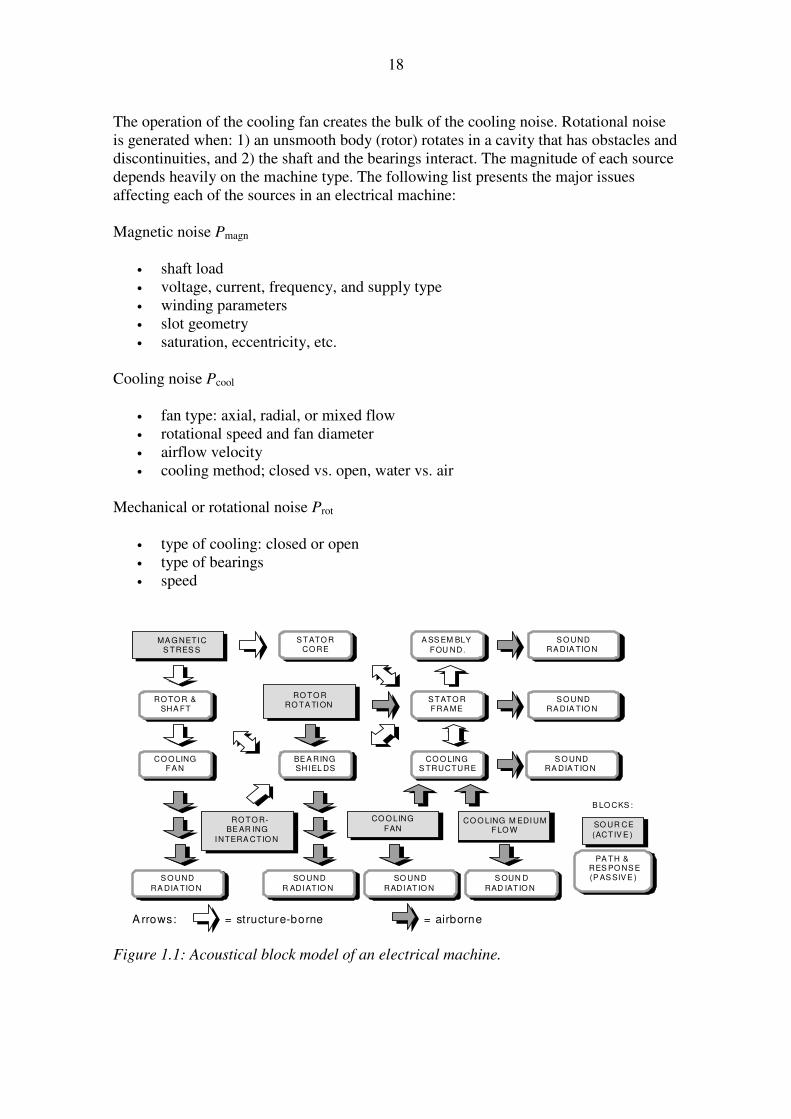
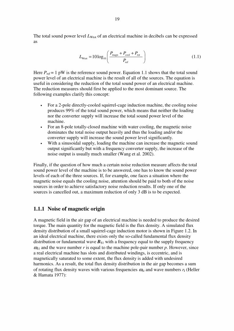

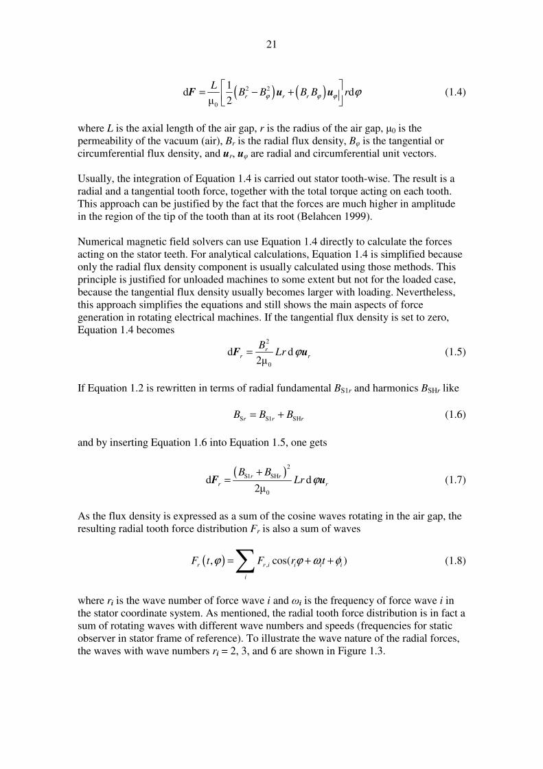


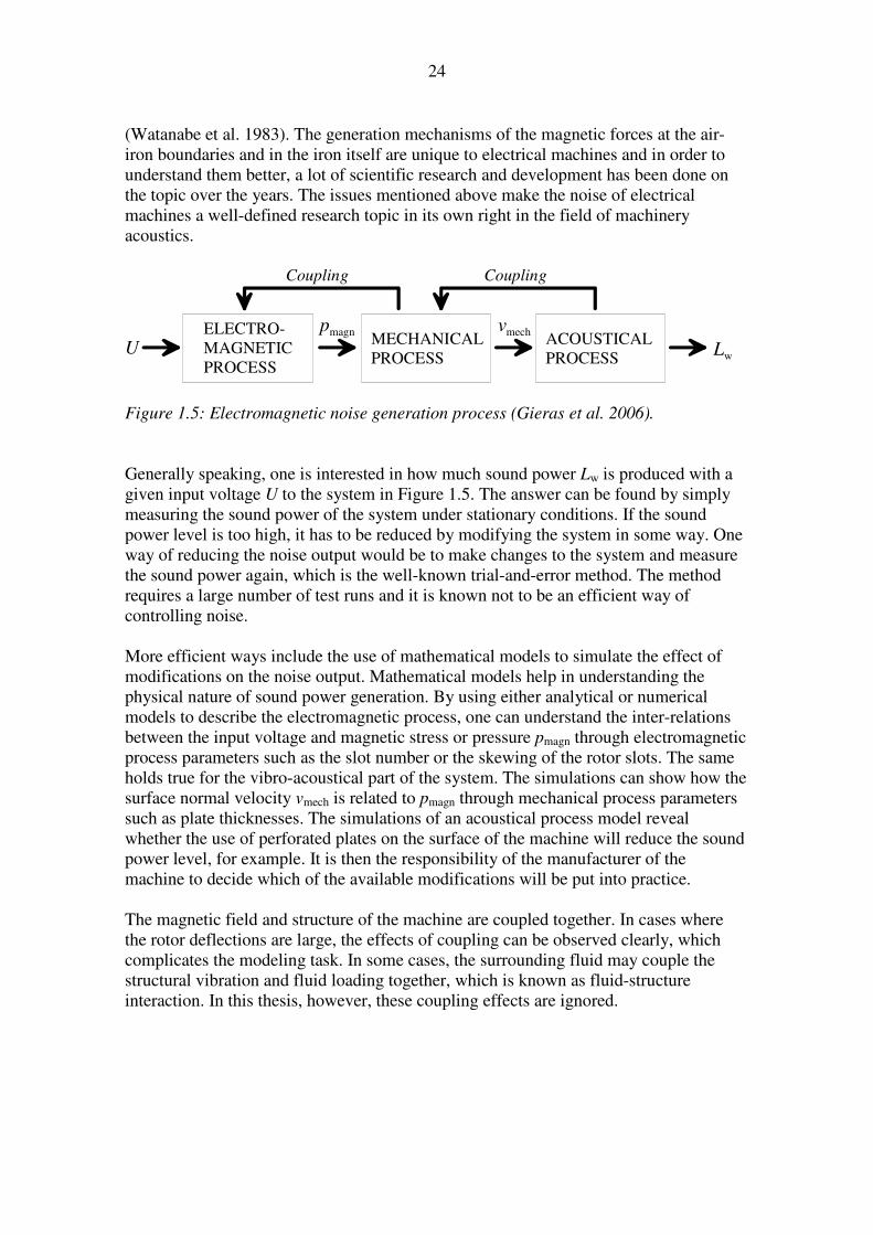


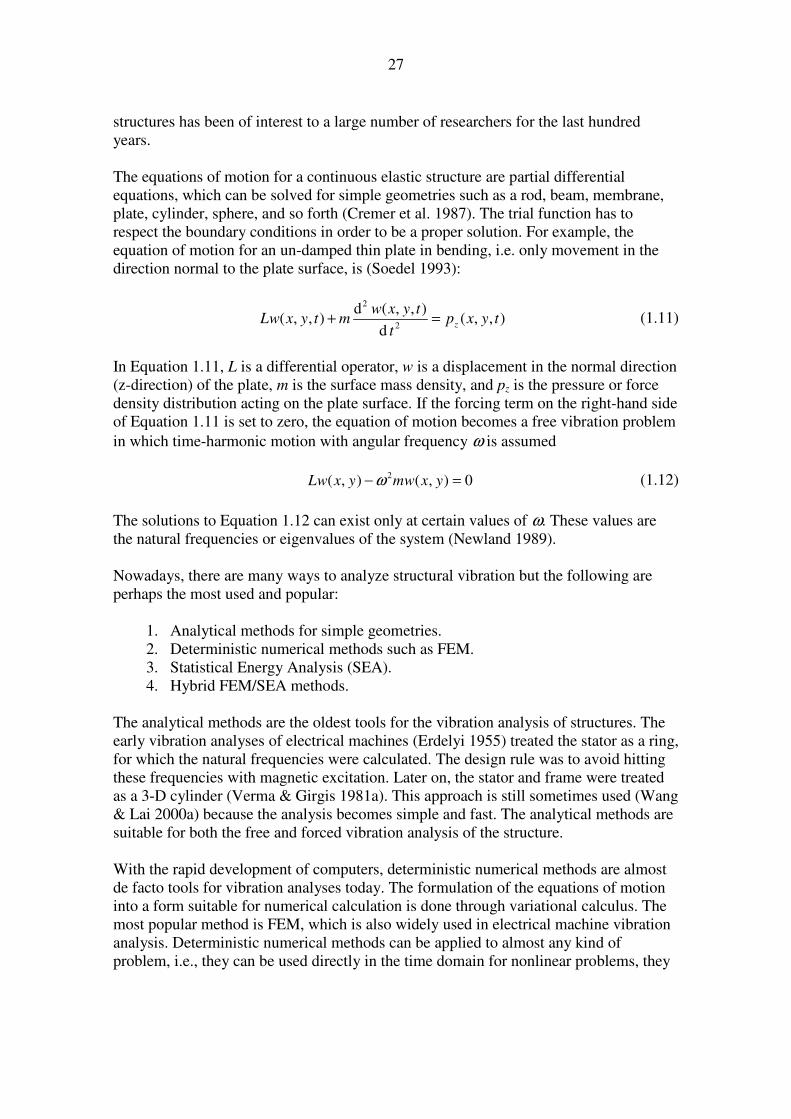


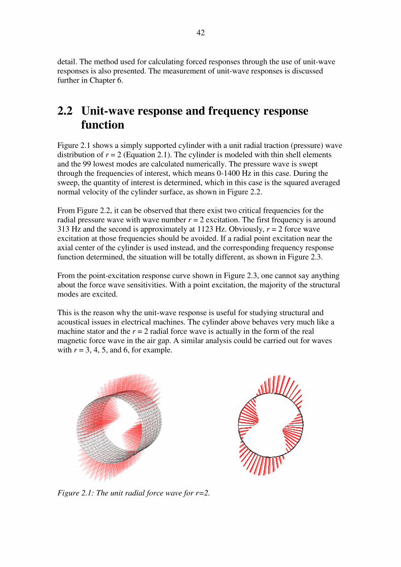


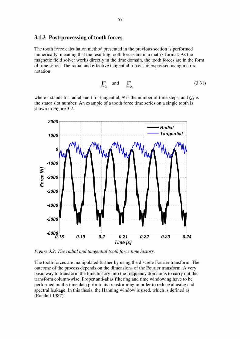

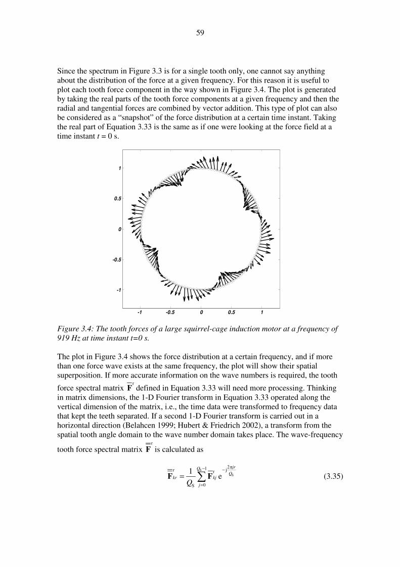


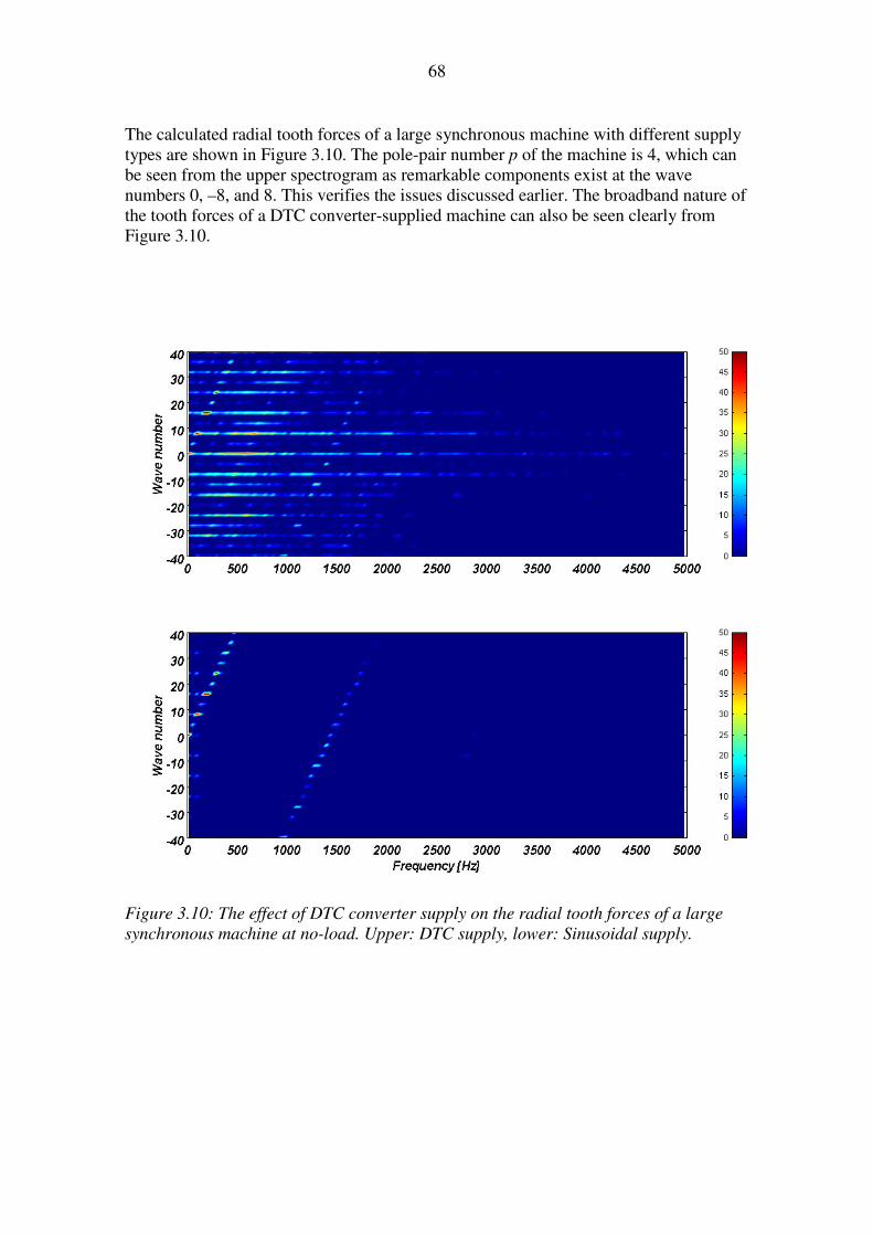
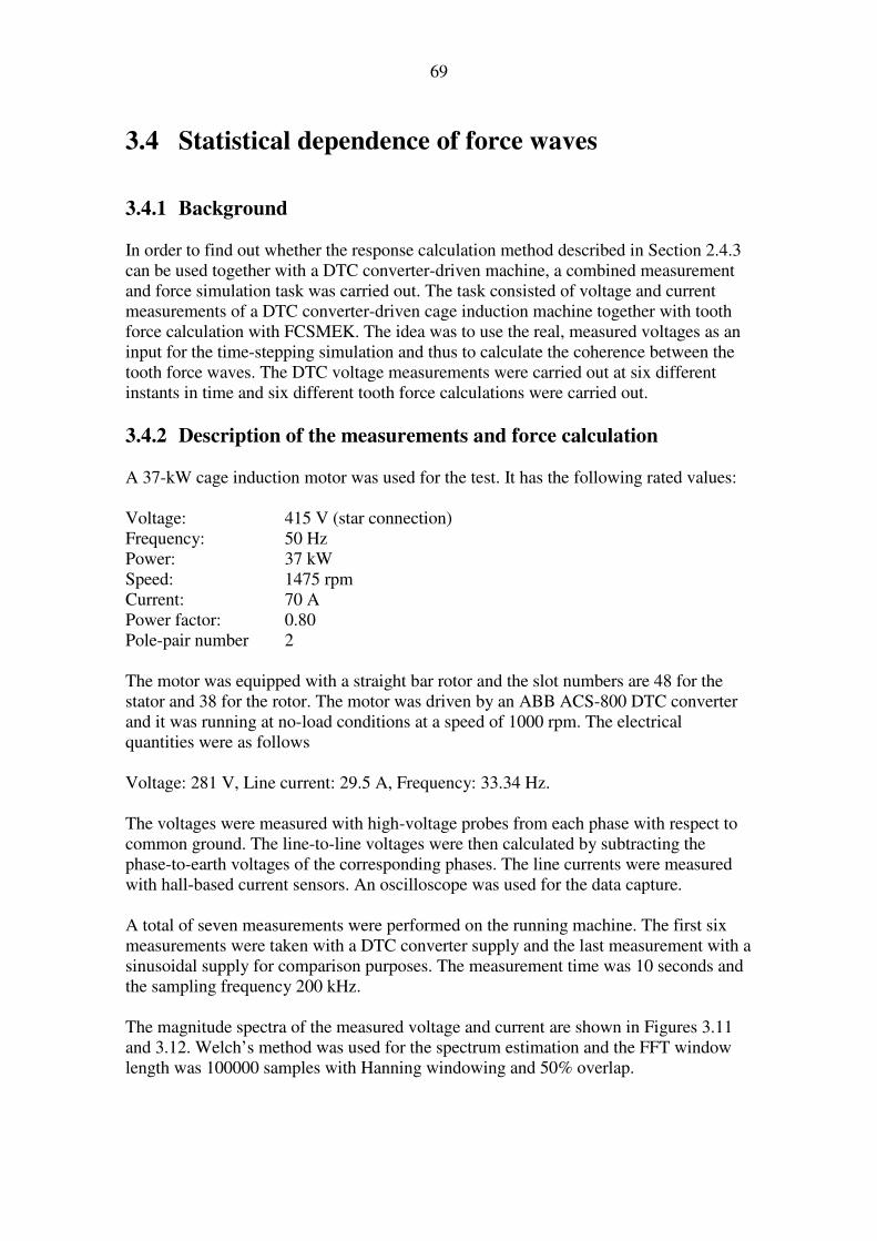


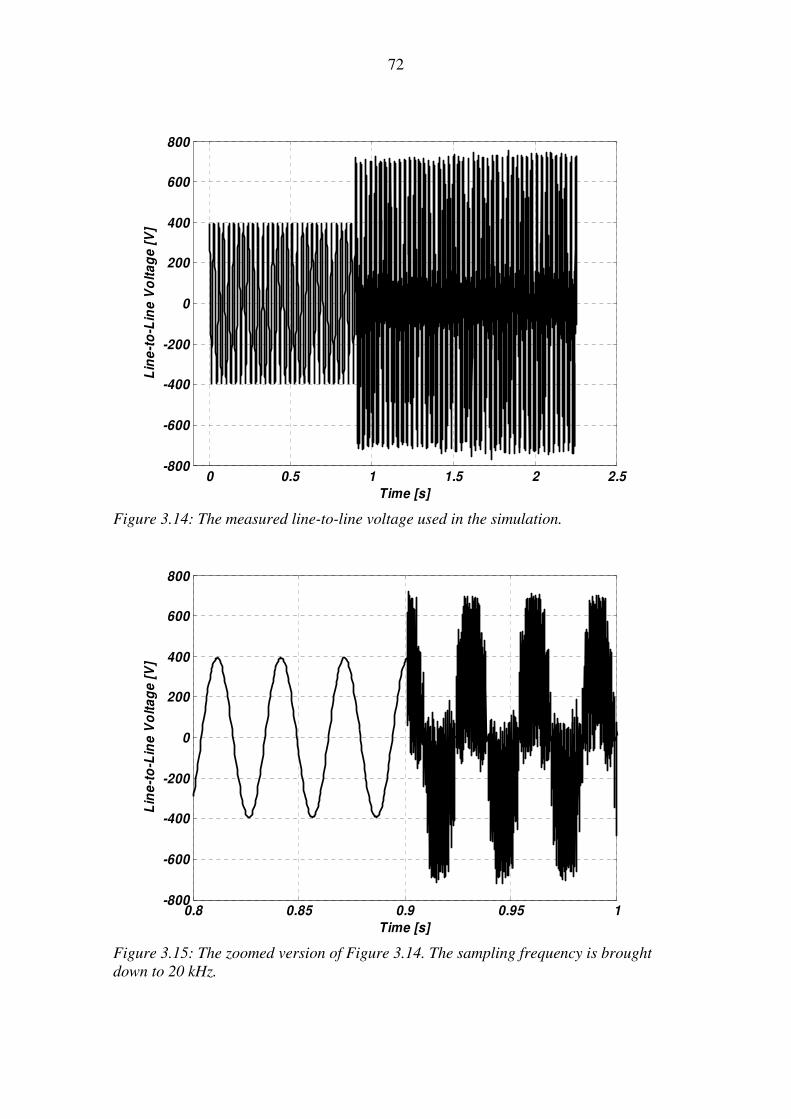


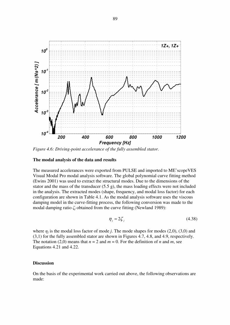


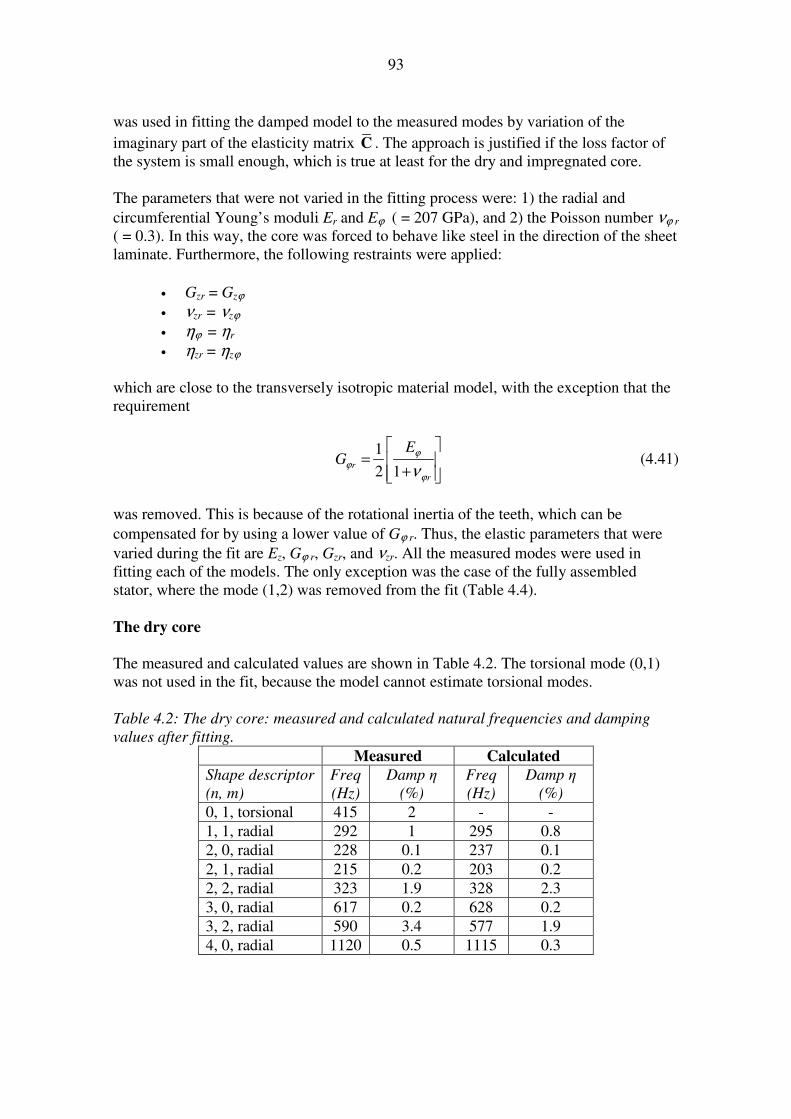


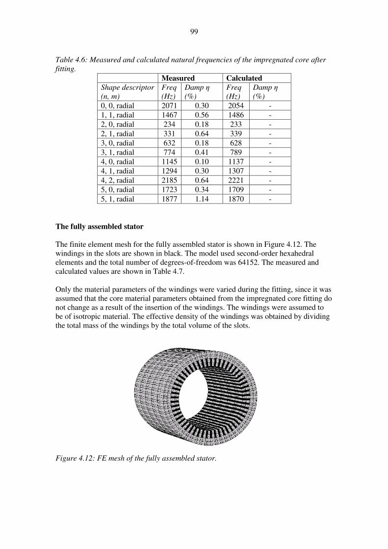
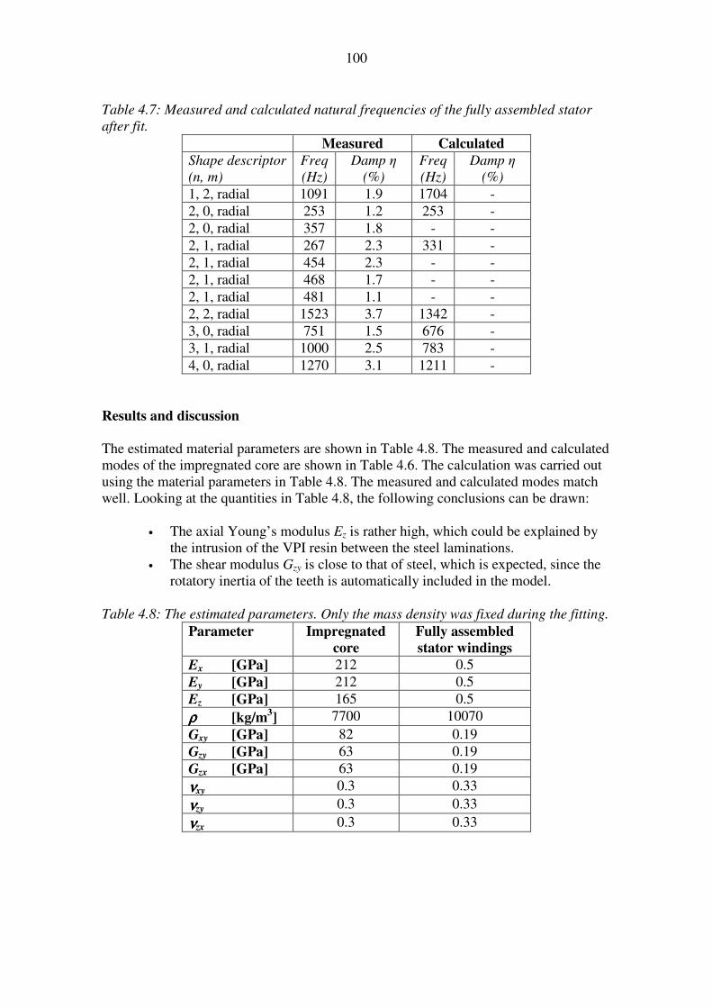


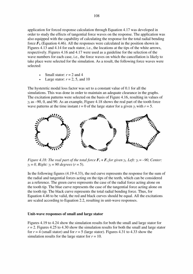


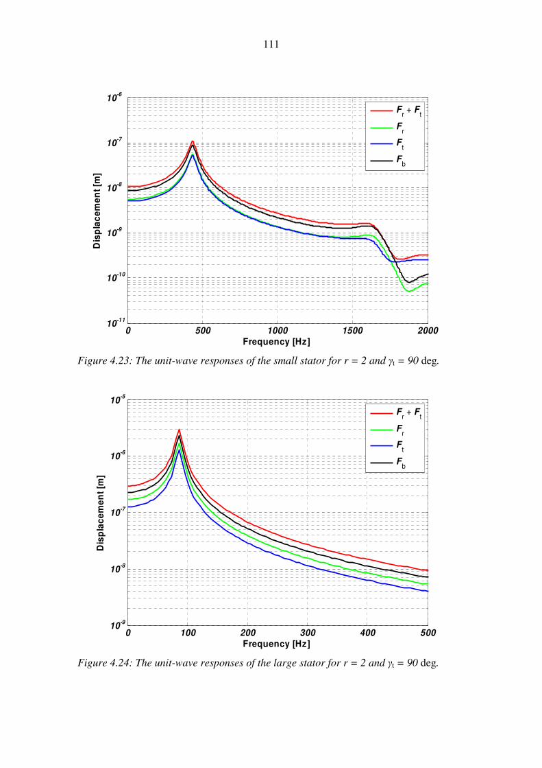


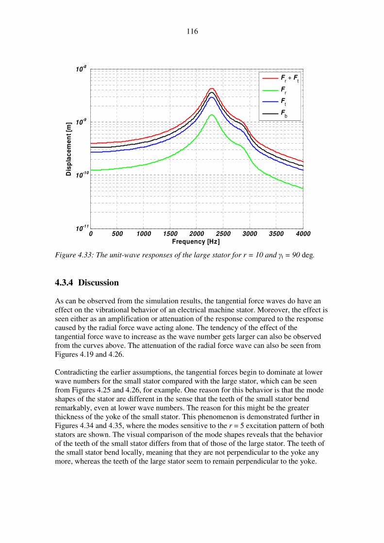
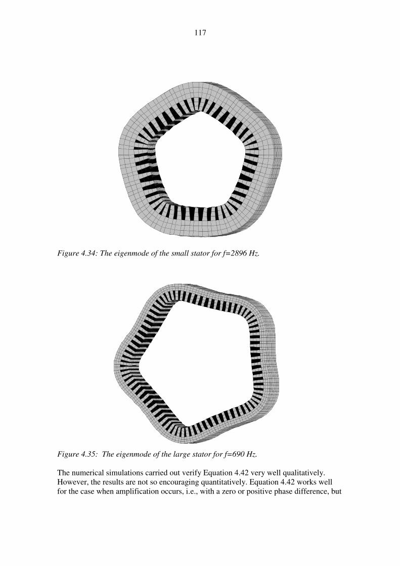

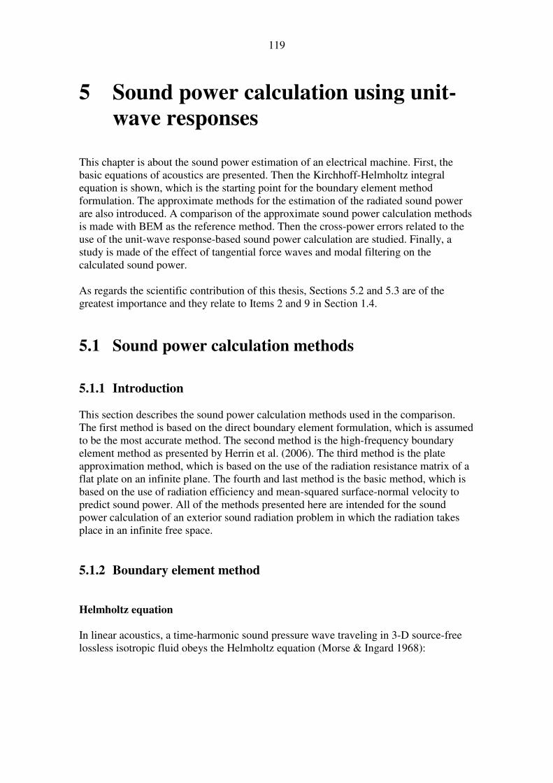


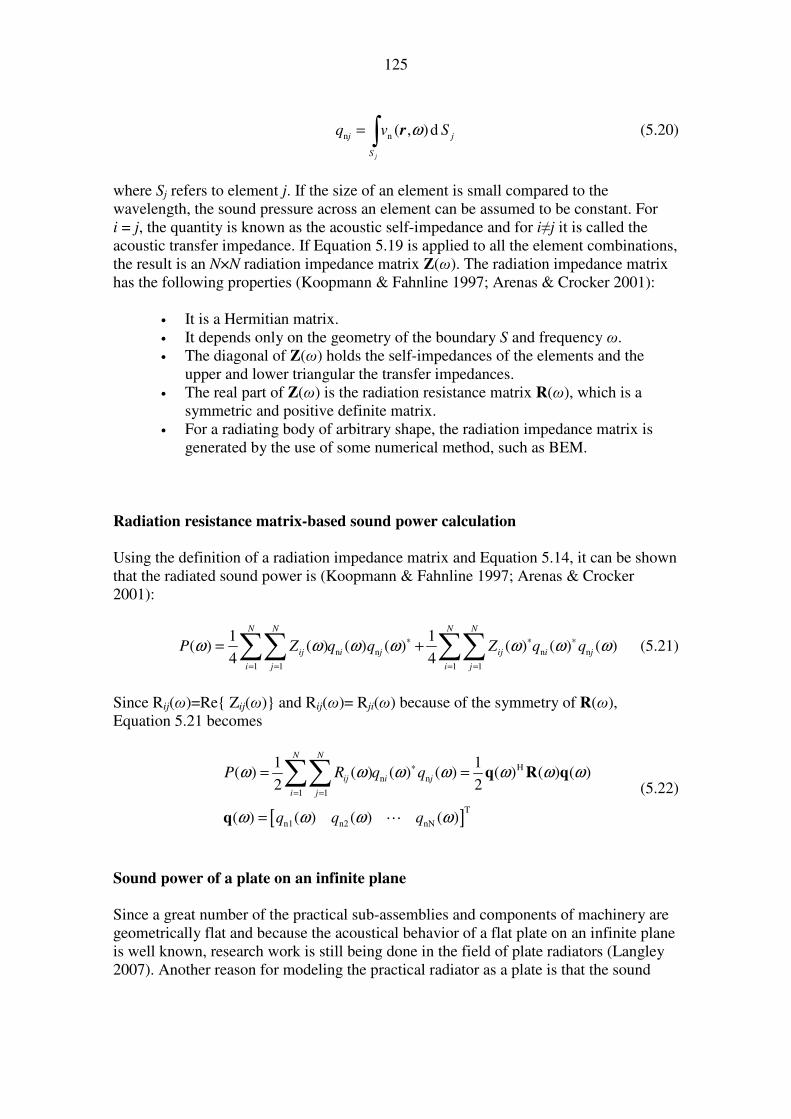
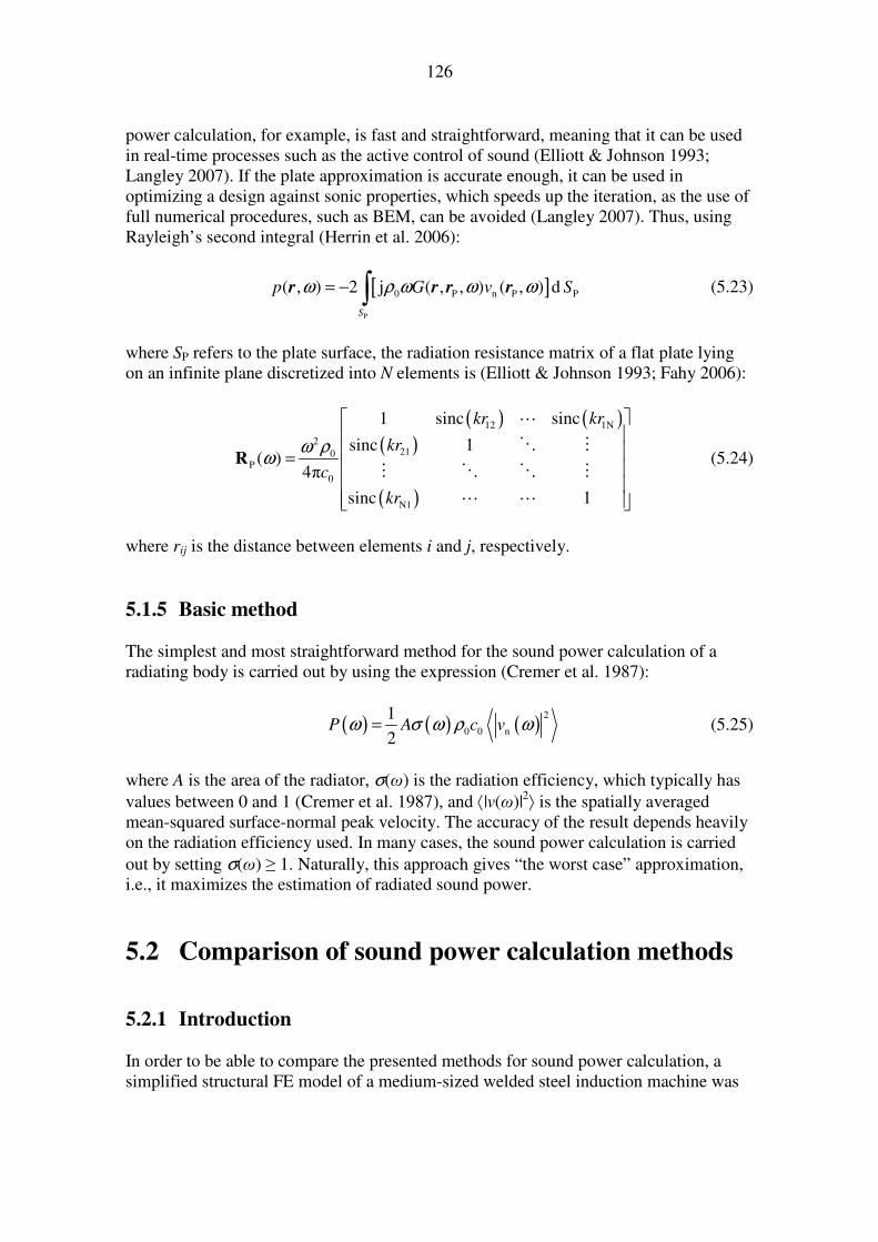
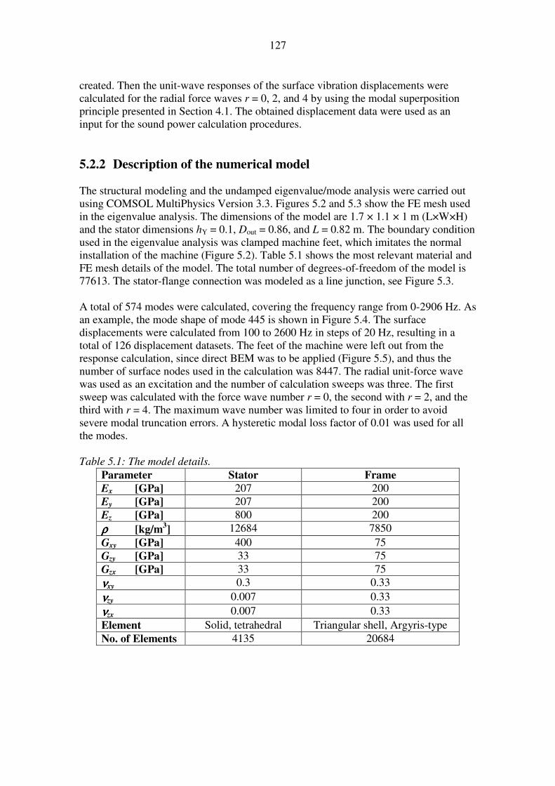


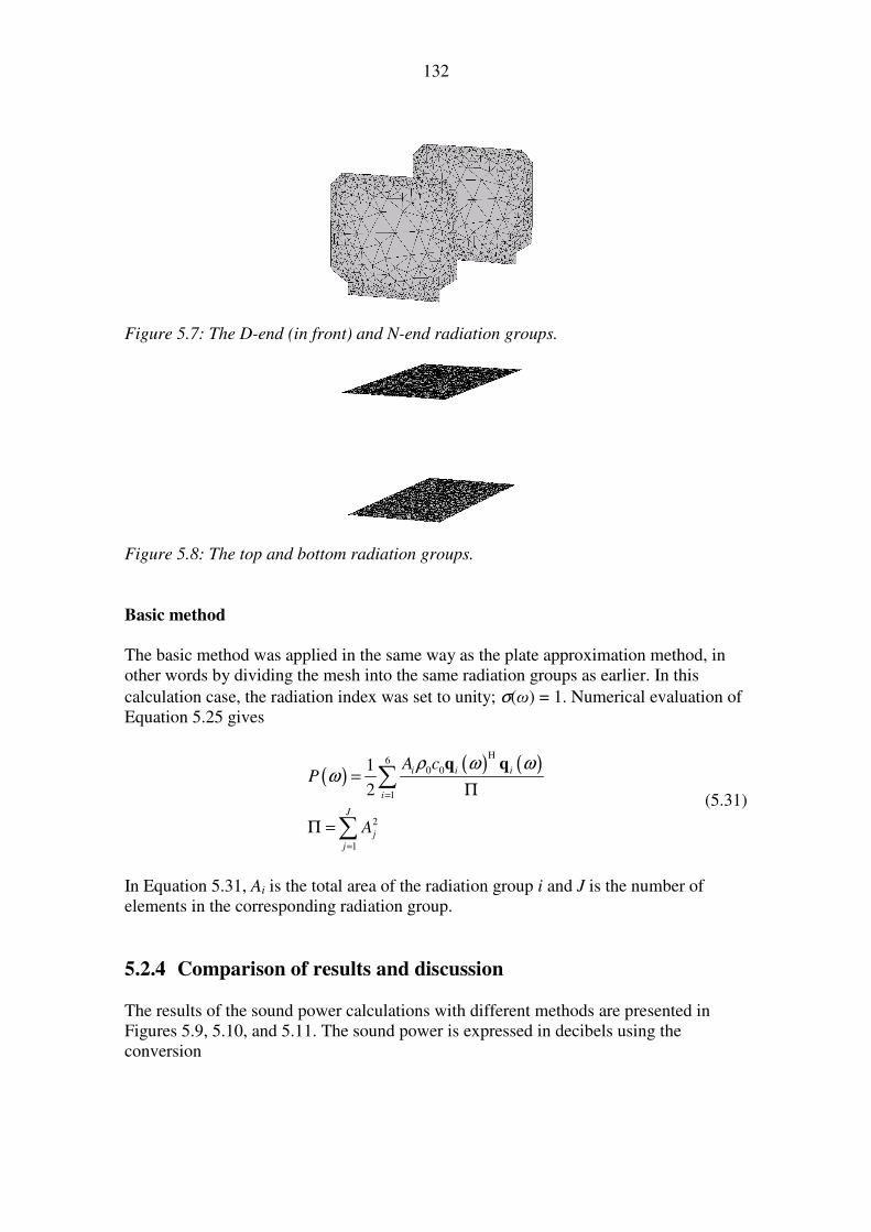
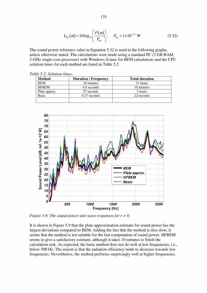


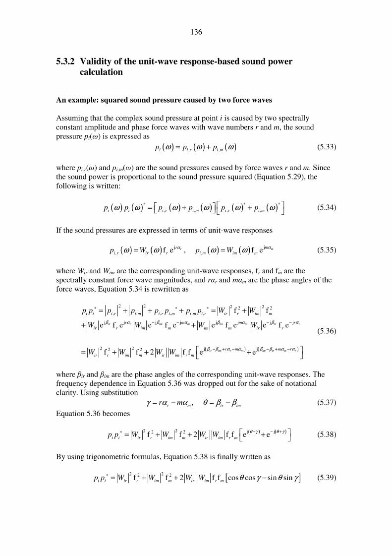

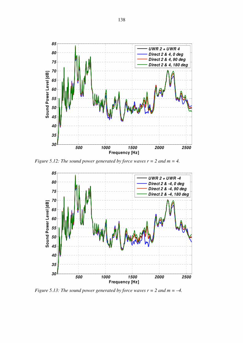


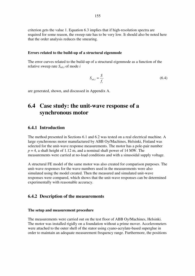

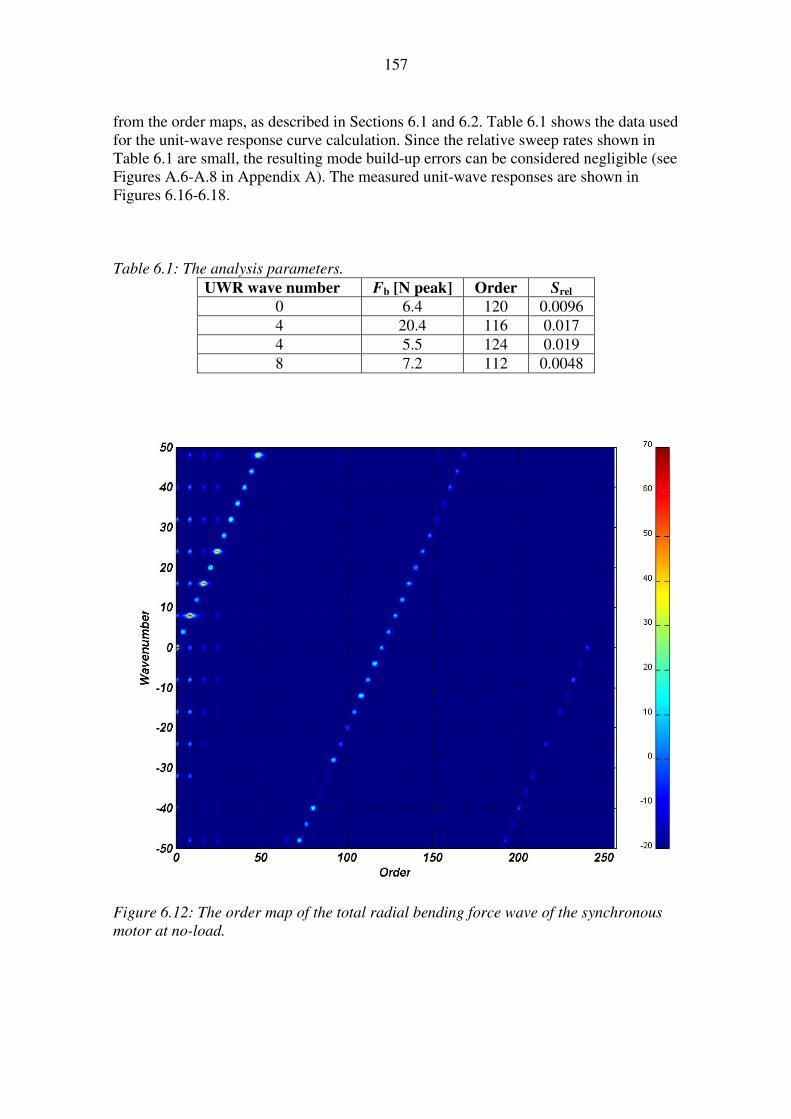


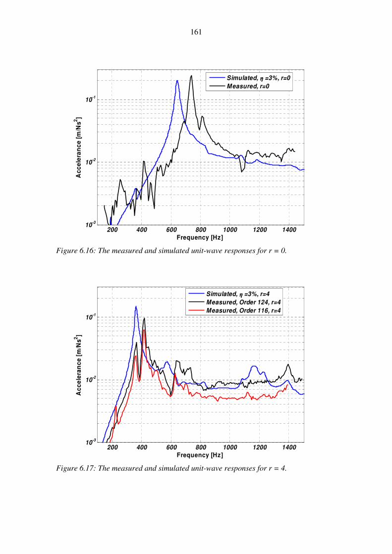


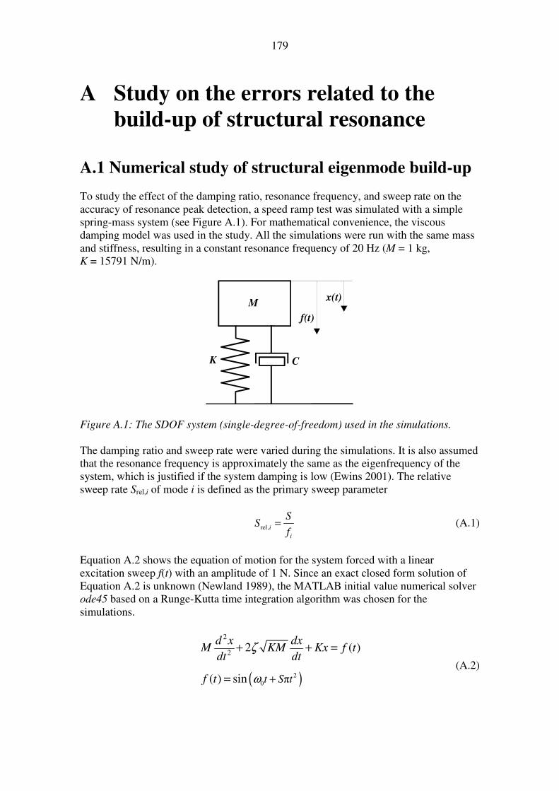


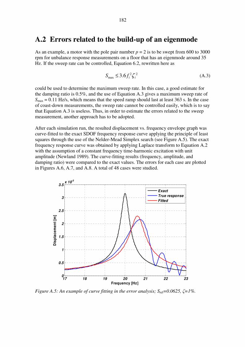


![Publication [IV] - TKK](https://static.documents.pub/doc/80x56/61f2fb971a17171fc95f7b67/publication-iv-tkk.jpg)


