July 12, 2010 January 29, 2001 January 29, 2001 January 29, 2001 January 29, 2001
United States: Selected Issues Paper This selected issues paper on United States was prepared by a staff team of the International Monetary Fund as background documentation for the periodic consultation with the member country. It is based on the information available at the time it was completed on July 12, 2010. The views expressed in this document are those of the staff team and do not necessarily reflect the views of the government of United States or the Executive Board of the IMF. The policy of publication of staff reports and other documents by the IMF allows for the deletion of market-sensitive information.
Copies of this report are available to the public from
International Monetary Fund Publication Services 700 19th Street, N.W. Washington, D.C. 20431
Prepared by Nicoletta Batini, Oya Celasun, Thomas Dowling, Marcello Estevão, Geoffrey Keim, Martin Sommer, and Evridiki Tsounta (all WHD)
Approved by Western Hemisphere Department
July 12, 2010
Contents Page
I. The Great Recession and Structural Unemployment ....................................................4 A. Introduction ...............................................................................................................4 B. Methodology .............................................................................................................5 C. Policy Implications ....................................................................................................7
II. Prospects for the U.S. Household Saving Rate ............................................................14 A. Introduction .............................................................................................................14 B. Experience of Nordic Economies ............................................................................14 C. Cross-Country Models of the Saving Rate ..............................................................15 D. What is the New Optimal Wealth Level? ...............................................................16 E. Conclusions .............................................................................................................16
III. Production and Jobs: Can We Have One Without the Other? .....................................22 A. Introduction .............................................................................................................22 B. How Does this Recession Compare to Previous Ones? ..........................................23 C. How Will the Recovery be Like? ............................................................................24 D. Conclusions and Policy Implications ......................................................................26
IV. The Financing of U.S. Federal Budget Deficits ...........................................................37 A. Introduction .............................................................................................................37 B. Post-Crisis Financing Patterns ................................................................................37 C. Baseline Projections of Demand for Treasury Debt ................................................38 D. A Model of Saving-Investment Flows ....................................................................39 E. Conclusions .............................................................................................................41
V. The U.S. Government’s Role in Reaching the American Dream ................................44 A. Introduction .............................................................................................................44 B. Impediments of the Current System ........................................................................45 C. Lessons from Other Countries.................................................................................46 D. Conclusions and Policy Implications ......................................................................48
2
VI. The U.S. Fiscal Gap: Who Will Pay and How? ...........................................................52 A. Introduction .............................................................................................................52 B. Methodology ...........................................................................................................52 C. Results .....................................................................................................................54 D. Conclusions .............................................................................................................56 A. What is the Fiscal Gap? ..........................................................................................63 B. What Are Generational Accounts? ..........................................................................63
Figures I. l. Increase in Skill Mismatch Index Since Onset of Recession .........................................9 I.2. Labor and Housing Market Dispersion ........................................................................10 I.3. Change in Foreclosure Rates, 2005–2009 ...................................................................11 I.4. Estimated Equilibrium Unemployment Rate at End-2009 by State ............................12 II.1. U.S. Household Saving Rate Adjustment Could be Protracted ...................................19 III.1. Real GDP Growth and the Change in the Unemployment Rate, 1902–2009 ..............28 III.2. Long-Term Unemployment Across U.S. Postwar Recessions ....................................28 III.3. Rolling Okun’s Law Coefficients and Growth Compatible with Stable
Unemployment, 1915–2009 .............................................................................29 III.4. Comparing the Steep Recessions and Job-Rich Recoveries ........................................30 III.5. Comparing the Most Recent Recessions and Jobless Recoveries ...............................31 III.6. Comparing the Great Depression and the Great Recession .........................................32 III.7. Stock Market Volatility versus Rolling Okun’s Law Coefficients ..............................33 III.8. Impulse Responses from a Tri-Variate SVAR.............................................................34 III.9. Unemployment Scenarios ............................................................................................35 V.1. Housing Finance in the United States and Other OECD Countries .............................50 VI.1. U.S. Debt in Percent of GDP (1930–2083)..................................................................60 VI.2. U.S. Federal Fiscal Overall (solid) and Primary Deficit (dotted) in Percent of GDP (1980–2083) .....................................................................................................60 VI.3. Total Revenues andTax Revenues in Percent of GDP—Advanced G-20 Countries ...61 Tables I.1. Explaining Changes in State-Level Unemployment Rates ............................................8 II.1. Household Saving Rate: Baseline Regression Results ................................................18 III.1. Estimating Labor Demand and Okun’s Law for a Panel of Countries ........................27 IV.1. Projections of Baseline Demand for U.S. Treasury Securities and the Impact of Excess Supply on Long-term Bond Yields..................................................42 V.1. United States and Canada: Housing Finance ...............................................................49 VI.1. Macroeconomic Assumptions Underlying Budget Projections ...................................57 VI.2 U.S. Fiscal Imbalance in Terms of the Present Discounted Value of GDP .................57 VI.3. Fiscal Imbalance in Terms of the Present Discounted Value of GDP, 3 Percent Discount Rate ...................................................................................................58 VI.4. Lifetime Net Taxes as a Share of Present Value of Labor Income under Different Scenarios, 3 Percent Discount Rate .................................................................58
3
VI.5. Impact on Fiscal Gap (as % of PVD of GDP) of Fiscal Adjustment by 2015 and of Cap on Medicare ..........................................................................................58 VI.6. Additional Percent Increase in Taxes and/or Cut in Transfers Necessary to Close the Fiscal Gap if Adjustment Starts in: ............................................................59 Appendices II.1. State-Space Model for Saving Rate and Wealth ..........................................................20 VI.1. Definition of Fiscal and Generational Gaps ................................................................63 Appendix Tables II.1. State-Space Model: Coefficient Estimates ..................................................................20
4
I. THE GREAT RECESSION AND STRUCTURAL UNEMPLOYMENT1, 2
This chapter examines the impact of regional skills mismatches and housing market hurdles on the national equilibrium rate of unemployment. The extreme regional disparities created by the crisis are associated with a 1 to 1¾ percentage points higher national equilibrium unemployment rate.
A. Introduction 1. The financial crisis has hit the U.S. labor market strongly, creating large regional disparities and unequally affecting different segments of the labor market. Not only have unemployment rates reached levels near post-World War peaks, but unemployment duration is at historic highs.3
The crisis affected some groups more severely, including men, youth, and low-skilled individuals and hit some sectors particularly hard, especially manufacturing, construction, and parts of the financial industry.
2. Such a high-magnitude shock—indeed the worst recession since the Great Depression—could have created structural labor market problems. In particular, some economic activities and states were much more affected by the crisis than others. The ability of the labor market to clear under these circumstances would depend on several factors, including: (i) the speed with which worker skills can be re-molded to changed demands; (ii) the flexibility of wages across the country and sectors; and (iii) the capital losses and credit constraints individuals would face if selling their houses or walking away from their underwater mortgages to migrate to more prosperous areas. Also, the monumental crisis has triggered decisive responses from the government, including increases in the generosity of unemployment insurance. While appropriate to cushion the recession, generous unemployment insurance benefits curb job-search intensity, thus cementing the upward pressures on equilibrium unemployment now and going forward if labor market slack is persistent. 3. This chapter shows that the crisis has created extreme disparities across states in terms of skill mismatches and housing market performance, which could have raised the national equilibrium unemployment rate by 1 to 1¾ percentage points. The analysis shows that the collapse in the housing market and the decline in the production of certain goods and services had a distinct regional pattern. More worrisome, we find that skill
1 Prepared by Thomas Dowling, Marcello Estevão, and Evridiki Tsounta.
2 Summary of forthcoming IMF Working Paper by Marcello Estevão and Evridiki Tsounta (both WHD). 3 There has been a trend increase in unemployment duration since the 1970s, partly explained by the passage of the baby boomers into their prime working years (Abraham and Shimmer, 2001), although the recent increase driven by the crisis is well beyond levels implied by the documented trend.
5
mismatches have been more acute in states with depressed housing markets—an interaction that is associated with even higher unemployment rates. Using a panel econometric model for the 50 states and the District of Columbia (controlling for the cyclical relationship between the unemployment rate, mismatches between supply and demand of labor skills, and housing market conditions) we find that the impact of skill mismatches and housing hurdles might have raised the national equilibrium rate of unemployment by 1 to 1¾ percentage points since 2007, with large regional variations in unemployment performance. However, our analysis does not directly imply that this structural increase in unemployment rates will persist; that depends on, among other factors, how quickly the skill mismatches and housing stress normalize.
B. Methodology 4. We construct an index for skill mismatches across the 50 states and the District of Columbia. The index captures how shrinking industries contribute to the swelling of a particular skill set among the unemployed, which may not necessarily be absorbed by expanding industries. The skill-mismatch index (SMI), following Peters (2000), measures the disparity between demand and supply at each skill level (according to educational attainment) in a state, with higher readings indicating greater mismatches. 5. Skill mismatches have risen sharply during this recession, with considerable heterogeneity across states (Figures 1 and 2). Mismatches are now near or at peak historical levels in numerous states, mostly the ones with a large manufacturing sector. States that had specific characteristics (e.g., Delaware—a financial hub; Hawaii—highly reliant on tourism; and Michigan—an auto hub) experienced disproportionate increases in skill mismatches. 6. The largest housing crash since the Great Depression has added to labor market frictions. The FHFA house-price index has declined by an average of 15 percent from its peak in 2007, with some states experiencing much larger declines (notably California, Florida and Nevada with declines of 35–50 percent), resulting in large disparities in the share of underwater mortgages.4 5 Foreclosure rates also suggest large dispersion in housing market conditions, with the national average at around 4½ percent, and foreclosure rates ranging from around 1 percent in Alaska and Wyoming to double-digit levels in Florida and Nevada (Figure 3).6
4 Our analysis is based on FHFA house prices given the better geographic coverage; our results remain robust to using Case-Shiller house-price indices.
Slower inter-state migration, likely related to the housing crash, seem to have
5 According to First American CoreLogic (2010), 70 percent of all mortgaged properties were underwater in Nevada at end 2010Q1, while less than 10 percent of the mortgaged properties in New York and Oklahoma had negative equity.
6 Foreclosure rates are strongly correlated with negative equity measures.
6
crimped the usual labor market adjustment mechanism in the United States (see Frey 2009 and Estevão and Tsounta, 2010). Even more worrisome, states that face housing market hurdles tend to also face disproportionately large increases in skills mismatches. 7. Econometric results confirm that regional skill mismatches and housing conditions could have raised unemployment rates. Table 1 shows that higher skill mismatches and foreclosure rates usually raise unemployment rates even after correcting for common cyclical factors. Skill mismatches would account for around 50 basis points of the increase in the national equilibrium unemployment rate since the end of 2007. A specification using the share of subprime mortgages in a state as an instrument for changes in foreclosure rates (to minimize any residual causality going from changes in unemployment rates to housing market conditions) confirm the findings. In addition, larger skill mismatches in states/years with bad housing conditions (and vice-versa) appear to be associated with higher unemployment rates than in the presence of milder housing cycles. 8. Our analysis suggests that increases in skill mismatches and deterioration in housing conditions explain a significant share of increased unemployment during the crisis. The specifications shown in Table 1 imply an increase in the national equilibrium unemployment rate (related to skill mismatches and housing conditions) between 2007 and 2009 ranging from 1 to 1¾ percentage points. Some states have experienced a large increase in structural unemployment factors (e.g., Florida, Arizona, Hawaii, and Nevada) while others have experienced only minor increases (e.g., D.C., West Virginia, Alabama, and the Dakotas) (Figure 4). A simple Hodrick-Prescott filter applied to state-level unemployment rate data and then aggregated at the national level using relative labor force shares as weights, produces a national equilibrium unemployment rate of about 5 percent in 2007—a level consistent with estimates by other analysts. Thus, the structural changes discussed here, imply an equilibrium unemployment rate in the United States of around 6½ percent in 2009. 9. Going forward, our estimates do not directly imply that this structural increase in unemployment rates will be persistent.7
7 Due to data limitations (the skills mismatch index begins in 1990) our analysis does not shed light on the persistence question, as the recessions of the early 1990s and early 2000s were shallow and did not post the same level of regional dislocation. The natural rate of unemployment has been on a decreasing trend since the mid-1970s (even during recessions), making persistence an important issue for future research.
The U.S. economy is quite flexible and it is possible that current skill mismatches in the labor market and structural problems in the housing markets would be cleared before too long. However, ongoing high mortgage delinquency rates and evidence of record-high rates of negative housing equity suggest that the woes in that sector may constrain labor mobility for a while. Also, the sharp rise in skill mismatches may have a deeper base than in previous downturns, as sector-specific shocks and the pressure to reallocate resources away from declining sectors to tradable goods sectors have been enormous.
7
C. Policy Implications 10. We find that equilibrium unemployment rates increased by about 1½ percentage points in the United States following the Great Recession, which calls for some policy action. The macroeconomic stimulus in the pipeline could be complemented by targeted policies to raise hiring and clear the housing market, though the fiscal costs of such policies should be closely evaluated given the concerns about the sustainability of the U.S. fiscal position. Priority could be given to subsidies to net hiring as academic research has shown such subsidies to be a more enduring way to raise employment rates, although these subsidies would need to be well targeted to limit redundancy and waste (Katz, 2010, and Estevão, 2007).8
8 Kitao, Sahin, and Song (2010) find that hiring subsidies and a payroll tax deduction can stimulate job creation in the short term but can cause a higher equilibrium unemployment rate in the long term.
Well-designed policies to enhance matching between vacancies and unemployed workers and to improve the skills of the unemployed could also help (Heckman, Lalonde, and Smith, 1999). Measures to raise the number of mortgage modifications, and if needed allowing mortgages to be renegotiated in courts (“cramdowns”), could also be important, as they would help to clear the housing markets more quickly.
8
(1) (2) (3) (4) (5) 2/ (6) 3/
Log-change in real GDP 4/ -0.05*** -0.05*** -0.04*** -0.04*** -0.05*** -0.03***(0.0) (0.0) (0.0) (0.0) (0.0) (0.0)
Log-change in skill mismatch index 3.2*** 2.6*** 2.4*** 1.7***(0.0) (0.0) (0.0) (0.0)
Log-change in skill mismatch*pp. change in foreclosure rate 1.9* 1.4(0.1) (0.6)
Time effects 5/ Yes Yes Yes Yes Yes Yes
Fixed state effects Yes Yes Yes Yes Yes Yes
Adj. R-squared 0.6 0.6 0.6 0.6 0.7 0.6
Number of states, including D.C. 51 51 51 51 51 51
Observations 918 918 918 918 918 867
Table 1. Explaining Changes in State-Level Unemployment Rates 1/
4/ The estimates are below those typically found in cross-country regressions (see Chapter III of this Selected Issues Paper), as expected when using a panel of U.S. states and time dummies. In this setup, changes in state GDP above and beyond the country average would pick up the ensuing labor mobility across states (a minor effect in cross-country regressions), which serves to equalize unemployment rates. State-by-state regressions, which would minimize (albeit not eliminate) this effect, produces an average Okun’s coefficient for the country as a whole of -0.22.
1/ Panel approach; annual data for the period 1990-2008 for 50 U.S. states plus the District of Columbia.
5/ Controls for business cycle variations and changes in national policies, e.g., policy interest rates.
3/ Instruments used: subprime share of mortgages (contemporaneous and 1-period lag), log-change of skill mismatch*share of subprime mortgages (contemporaneous and 1 lag).
*Significant at a 10 percent level of significance, **significant at a 5 percent level of significance, ***significant at a 1 percent level of significance.
Dependent variable: percentage-point change in unemployment rate
(numbers in parentheses are p-values)
OLS 2SLS
2/ Instruments used: subprime share of mortgages (contemporaneous and 1 period lag).
9
(in percent)
Figure 1. Increase in Skill Mismatch Index Since Onset of Recession(in percent)
Sources: Haver Analytics, U.S. Bureau of Labor Statistics, U.S. Census Bureau, and authors’ calculations.
Notes: 1st quartile [-11.1,5.7], 2nd quartile [6.3,11.6], 3rd quartile [12.3,16.9], 4th quartile [17.2,29.4]. Calculated as the percent change from 2007–2009. Annual levels are the simple average of 12 months.
○1st quartile (best)
●2nd quartile
●3rd quartile
●4th quartile (worst)
10
Figure 2. Labor and Housing Market Dispersion
Sources: Haver Analytics, Mortgage Bankers Association, U.S. Bureau of Labor Statistics, U.S. Census Bureau, U.S. Federal Housing Finance Agency House Price Index, and authors' calculations.1/ Weighted average annual percentage change in Skill Mismatch Index weighted by size of state labor force.
National simple average FHFA house price index, 1990=100, SA1 standard deviation
FHFA House Price Dispersion
11
Sources: Mortgage Bankers Association, and authors’ calculations.
Notes: 1st quartile [0.6,0.96], 2nd quartile [0.97,1.56], 3rd quartile [1.6,2.69], 4th quartile [2.7,11.7]. Calculated as the percentage point change from 2005-2009. Annual levels are the simple average of 12 months.
Figure 3. Change in Foreclosure Rates, 2005–2009(in percentage points)
○1st quartile (best)
●2nd quartile
●3rd quartile
●4th quartile (worst)
○1st quartile (best)
●2nd quartile
●3rd quartile
●4th quartile (worst)
12
Figure 4. Estimated Equilibrium Unemployment Rate at End-2009 By State 1/(in percent)
Sources: U.S. Bureau of Labor Statistics and authors' calculations.1/ Equilibrium unemployment rate in 2007 is estimated using an HP-f ilter for the period 1990-2007 for each state. The structural increase in the unemployment rate in 2008 and 2009 is the increase in the f itted unemployment rate value, as predicted by the model, f rom the increases in skills mismatches and housing hurdles. Note: States are ordered based on the cumulative structural increase in the period 2008-2009.
0
2
4
6
8
10
12
FL NV AZ CA HI MD DE ID NJ MI IN WI IL UT OR RI NM
REFERENCES Abraham, K.G. and R. Shimmer, 2001, “Changes in Unemployment Duration and Labor
Force Attachment,” NBER Working Paper No. 8513, National Bureau of Economic Research.
Estevão, M., 2007, “Labor Policies to Raise Employment,” IMF Staff Papers, Vol. 54, No.
1, pp. 113–138, March. Estevão, M. and E. Tsounta, 2010, “Is U.S. Structural Unemployment on the Rise?” IMF
Working Paper, forthcoming. First American CoreLogic, 2010, Negative Equity Report, May. Frey, W.H., 2009, “The Great American Migration Slowdown: Regional and Metropolitan
Dimensions,” Washington DC: Brookings Research Report, December. Government Accountability Office (2007), “Trade Adjustment Assistance: Changes to
Funding Allocation and Eligibility Requirements Could Enhance States’ Ability to Provide Benefits and Services,” GAO-07-701, Washington, DC: GAO.
Heckman, J., R. Lalonde, and J. Smith, 1999, “The Economics and Econometrics of Active
Labor Market Programs,” in O. Ashenfelter and D. Card (eds.), Handbook of Labor Economics, Elsevier Science.
Katz, L., 2010, “Long-Term Unemployment in the Great Recession,” Testimony Before the
Joint Economic Committee of the Congress of the United States, April 29. Kitao, S., A. Sahin, and J. Song, 2010, “Subsidizing Job Creation in the Great Recession,”
Federal Reserve Bank of New York Staff Reports, No. 451, May. Peters, D., 2000, “Manufacturing in Missouri: Skills-Mismatch,” ESA-0900-2. Research and
Planning, Missouri: Department of Economic Development, available at: http://www.missourieconomy.org/industry/manufacturing/mismatch.stm
This chapter assesses the prospects for U.S. personal saving in light of the sharp contraction of consumer spending during the financial crisis. Using two alternative econometric approaches, the paper finds that the saving rate may increase somewhat from current levels to about 4¾–5½ percent of disposable income in the medium term.
A. Introduction
1. During the early stages of the financial crisis, consumers sharply curtailed their spending. The saving rate jumped from 1 percent of disposable income in Q1/2008 to 5½ percent in Q2/2009 on the back of slumping asset prices, unprecedented uncertainty, and rapidly tightening credit conditions. Real personal consumption expenditures fell for two consecutive years during 2008–09—the first time since the Great Depression. However, with the diminishing tail risks and higher financial asset values, consumers have become somewhat less cautious in recent months. The saving rate has fallen to around 3–4 percent of disposable income, supporting a tentative recovery in consumer spending. Against this background, this Chapter examines the prospects for the U.S. household saving rate.
B. Experience of Nordic Economies
2. The historical record of Finland, Norway and Sweden provides a cautionary tale. Similarly to the United States, these economies experienced joint asset price and banking busts in the late 1980s. In the aftermath of the crises, the personal saving rate tended to remain elevated for many years (Figure 1). The trough-to-peak increase in saving was considerable—between 5–10 percentage points of disposable income.
3. In the United States, the run up in the saving rate has so far been smaller than in the Nordic economies. This may reflect a variety of factors. The extraordinary policy response in the U.S. quickly eliminated tail risks, and asset prices stabilized much faster than in Nordic economies, after about a year. The initial imbalances in the household sector were also by some measures less pronounced in the United States—the pre-crisis saving rates were negative in Nordic economies, between -2 and -4 percent of disposable income.2
4. However, the historical experience of Nordic countries also suggests that consumer deleveraging can take a long time—between 6 and 8 years. One notable feature of the U.S. developments so far is that household indebtedness has fallen little from its
1 Prepared by Martin Sommer with contributions from Jirka Slacalek.
2 In addition, the Nordic economies continued to be pummeled by external shocks (economic transition in the CEECs, exchange rate volatility), their inflexible economies went through a period of labor and product market liberalization, and domestic asset prices fell for at least 4 consecutive years.
15
historical peak (Figure 1), while lending standards remain very tight. This would point to the need to maintain the U.S. household savings at a much higher level than during the pre-crisis period.
C. Cross-Country Models of the Saving Rate
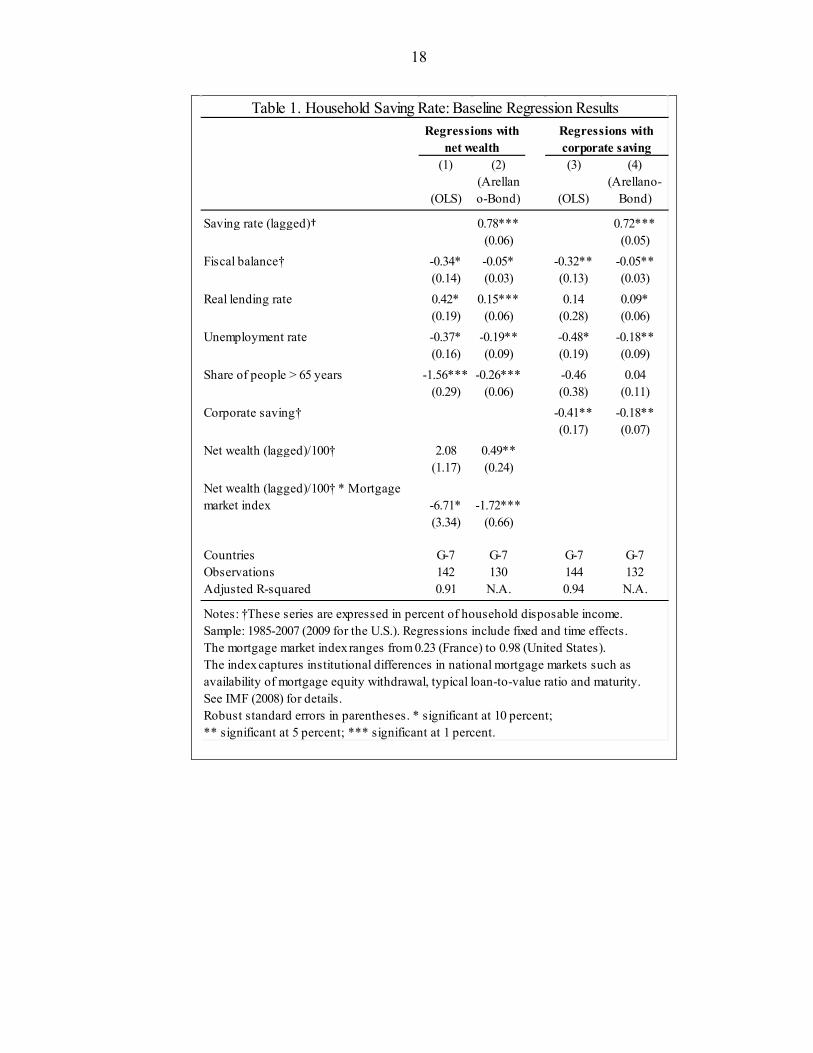
5. To assess prospects for household saving, staff estimated two alternative econometric models—panel regressions and a state-space system. The panel regressions link personal saving to a range of fundamentals such as wealth, corporate saving, interest rates, fiscal policy, and demographics (Table 1).3
6. The panel regressions suggest that the personal saving rate will remain elevated and could under plausible assumptions increase to about 4¾–5½ percent of disposable income in the medium term.
4
• Wealth. With future asset price growth likely subdued (and continued downside risks to house prices), consumers will need to save to rebuild their net wealth, which at 500 percent of disposable income remains well below the average of the past 20 years (533 pct of disposable income). This factor contributes over 2½ percentage points to the predicted net increase in the saving rate from 1¾ percent in 2007 to 4¾–5½ percent in 2018 when the economy returns back to potential (Figure 1).
• Fiscal policy and interest rates. Persistent large fiscal deficits will affect consumer behavior in two ways—higher interest rates will stimulate saving, while expectations of future tax increases may encourage some consumers to spend less relative to their current income. The higher prospective deficits and interest rates contribute over 2¼ percentage points to the predicted increase in the saving rate.
• Demographics. In contrast, retirement of the baby-boomer generation over the next several years could reduce the U.S. saving rate by more than 2 percentage points. That said, the demographic effects could be somewhat weaker in the current environment, as some employees will need to work beyond their normal retirement age to replenish the wealth lost from their defined-contribution pension plans.
• Cyclical effects. Cyclical factors such as the unemployment rate do not play a large role when decomposing the predicted changes in the saving rate between 2007 and 2018.5
3 The sample consists of the G-7 data over 1985–2007 (2009 for the United States).
However, the cyclical effects should boost the saving rate between now and
4 Deutsche Bank (2009) and Lee, Rabanal, and Sandri (2010) also find that the personal saving rate may settle above present levels in the medium term.
5 The unemployment rate is projected at close to 5 percent in both years.
16
the end of forecast period, as the unemployed who find a job in the future will be able to save more.
7. Uncertainty around the baseline saving rate projection is significant. For example, asset prices could rebound more strongly than expected, while robust foreign demand for the Treasury bonds could keep the yields and lending rates low. The households would then rebuild their balance sheets mostly through higher asset prices and the saving rate could be lower than under the baseline (Figure 1). Alternatively, ambitious fiscal consolidation could also reduce the household saving rate by limiting Ricardian effects and putting a ceiling on future interest rate increases.
D. What is the New Optimal Wealth Level?
8. Besides the uncertainty about future asset values, there is also little clarity about what consumers currently consider to be a “normal” level of assets, which provides them with an acceptable insurance against unexpected events. Staff therefore estimated an alternative model of U.S. “target wealth”, in which consumers tend to save more whenever the actual wealth is below the “target”, and vice versa (see Appendix). The target wealth is identified using a state-space model where the target wealth depends on the real interest rate and a statistical measure of uncertainty. Besides the deviation of actual wealth from the target, the household saving rate is also assumed to be affected by credit conditions and interest rates.
9. The model suggests that the target wealth has increased during the financial crisis. In the immediate pre-crisis period, the target net wealth was unusually low—well below 500 percent of disposable income—given the low interest rates and “great moderation”, i.e., an unusual drop in macroeconomic volatility. The large gap between actual and target wealth combined with loosening credit conditions explain why the saving rate fell so low during the 2000s (Figure 1). Since the onset of the crisis, the target wealth has increased considerably given large uncertainties, and could stabilize around 540–550 percent of disposable income once interest rates normalize. The medium-term saving rate predicted by the model is about 5¼ percent.
E. Conclusions
10. Despite the recent decline of the personal saving rate, households are not likely to return to their pre-crisis spending habits. While uncertainty has diminished and financial conditions have eased, the structural need to rebuild balance sheets, high fiscal deficits, and higher interest rates could raise the household saving rate in the medium term. The recent policy proposals to automatically set-up retirement plans and provide tax breaks for matching employer contributions could also boost saving (Economic Report of the President, 2010).
17
11. That said, the near-term dynamics of the saving rate is uncertain for a variety of reasons. In addition to the factors discussed above, the planned tax increases for upper-income households could reduce disposable income growth, thereby putting downward pressure on aggregate saving (but also on consumption). On the other hand, corporate profitability has remained strong and higher dividend payments could facilitate more saving in the near term. All in all, a significant decline in the saving rate appears unlikely and, given the expectations of slow recovery in the labor market, consumption growth will remain sluggish relative to the trends during previous recoveries.
Notes: †These series are expressed in percent of household disposable income.Sample: 1985-2007 (2009 for the U.S.). Regressions include fixed and time effects.The mortgage market index ranges from 0.23 (France) to 0.98 (United States).The index captures institutional differences in national mortgage markets such as availability of mortgage equity withdrawal, typical loan-to-value ratio and maturity. See IMF (2008) for details.Robust standard errors in parentheses. * significant at 10 percent;** significant at 5 percent; *** significant at 1 percent.
Table 1. Household Saving Rate: Baseline Regression ResultsRegressions with
net wealthRegressions with corporate saving
19
Figure 1. U.S. Household Saving Rate Adjustment Could Be Protracted
0
2
4
6
8
10
12
0
2
4
6
8
10
12
0 1 2 3 4 5 6 7
U.S. WEO projectionNorwaySwedenFinland
Note: Diamond corresponds to the first year of banking crisis. The first year of housing/stock market bust (t=0): Norway (1988), Sweden (1990), Finland (1989), United States (2007).
50
75
100
125
150
175
200
50
75
100
125
150
175
200
-6 -5 -4 -3 -2 -1 0 1 2 3 4 5 6 7 8
FinlandNorwaySwedenU.S.
Sources: IMF, World Economic Outlook; OECD; Norges Bank; Statistics Finland; Riksbank.
0
2
4
6
8
10
0
2
4
6
8
10
1985 1990 1995 2000 2005 2010 2015
Saving rateModel with net wealthModel with corporate saving
-4
-3
-2
-1
0
1
2
3
4
Note: Fiscal policy = contribution of the budget deficit; business cycle = contribution of the unemployment rate; demographics = contribution of population aged over 65 years, wealth effects = contribution of wealth-to-income ratio and wealth-to-income ratio interacted with mortgage market index.
Changein saving
rate
Fiscal policy(direct
channel)
Realinterest
rate
Businesscycle
Demographics
Wealtheffects
-6
-4
-2
0
2
4
6
Note: Fiscal policy = contribution of the budget deficit; usiness cycle = contribution of the unemployment rate; demographics = contribution of population aged over 65 years, wealth effects = contribution of wealth-to-income ratio and wealth-to-income ratio interacted with mortgage market index.
Changein saving
rate
Fiscal policy(direct
channel)
Realinterest
rate
Businesscycle
Demographics
Wealtheffects
300
400
500
600
700
300
400
500
600
700
1966Q3 1978Q3 1990Q3 2002Q3
95% Confidence Interval
68% Confidence Interval
ActualWealth
TargetWealth
Household Saving Rate after Banking and Housing Busts(pct point deviation from first year of housing/stock bust)
Household Debt in Percent of Disposable Income(pre-crisis peak at t=0: 100)
Saving Rate Projections Decomposition of the Decline in Saving Rate(1997-2007, percentage points)
Decomposition of the Predicted Increase in Saving Rate(2007-18, percentage points)
Estimate of Target Net Wealth
20
Appendix 1. State-Space Model For Saving Rate and Wealth In this specification, the saving rate depends on the deviation of household wealth from its (unobserved) target m-m*, credit conditions CC (approximated by banks’ willingness to extend consumer credit), and real interest rate r:
*t 0 m t ts = + ( - ) .s
t r t tm m ccCC rβ β γ γ ε+ + +
Consistent with the precautionary saving literature, the unobserved target wealth is modeled as a function of uncertainty δσ (measured by the Bloom’s index6
𝑚𝑡∗ = 𝛿𝜎 𝜎𝑡−12∗ + 𝛿𝑟 𝑟𝑡−1∗ + 𝜗𝑡𝑚
) and real interest rates:
It is assumed that the gap between actual and target wealth can be highly persistent:
*t = + .m
t tm m ε
1 = + .m mt t t
ε εε θ ε η− Realistically, the measured variables track the “true” underlying uncertainty and expected real interest rates (denoted by stars) only imperfectly:
2 2*= ,t t tσσ σ ε+
*
t = .rt tr r ε+
The resulting state-space system is estimated using the U.S. quarterly data during 1966–2009. The estimated coefficients are reported in the table below. Figure on the next page plots the estimated path for target household wealth.
Table 1. State-Space Model: Coefficient Estimates
β0 βm γCC γr δσ δr 10.046***
(0.825) -1.134***
(0.382) -6.905***
(1.020) 0.173
(0.176) 3.029*** (0.476)
0.293* (0.161)
Note: Standard errors are reported in parentheses. Star notation is the same as in Table 1.
6 The Bloom (2009) index combines information about stock market volatility, distribution of firm-level and industry-level growth rates, unemployment, and other relevant variables.
21
REFERENCES Bloom, Nicholas, 2009, “The Impact of Uncertainty Shocks,” Econometrica, 77(3), p. 623–
685. Economic Report of the President, 2010, “Saving and Investment”, Chapter 4 (Washington,
D.C.). Deutsche Bank, 2009, “Consumer Balance Sheet Adjustment: Half Way Done” (New York,
NY). International Monetary Fund, 2008, “The Changing Housing Cycle and The Implications for
Monetary Policy”, Chapter 3 of World Economic Outlook (Washington, D.C.). Lee, Jaewoo, Pau Rabanal, and Damiano Sandri, 2010, “U.S. Consumption after the 2008
Crisis”, IMF Staff Position Note 10/01, January (Washington, D.C.).
22
III. PRODUCTION AND JOBS: CAN WE HAVE ONE WITHOUT THE OTHER?1
This chapter examines whether the recovery will be accompanied by significant job creation or will be “jobless” like the previous two U.S. recoveries. It compares the recent recession with previous episodes and employs panel and time-series regressions to pin down the fundamental factors underlying the relationship between growth and (un)employment. The recent crisis has destroyed more jobs than any other post-Depression episode. However, if economic uncertainty recedes significantly, employment should rebound more strongly when compared to past jobless recoveries; although probably not strong enough to prevent a slow decline in the unemployment rate.
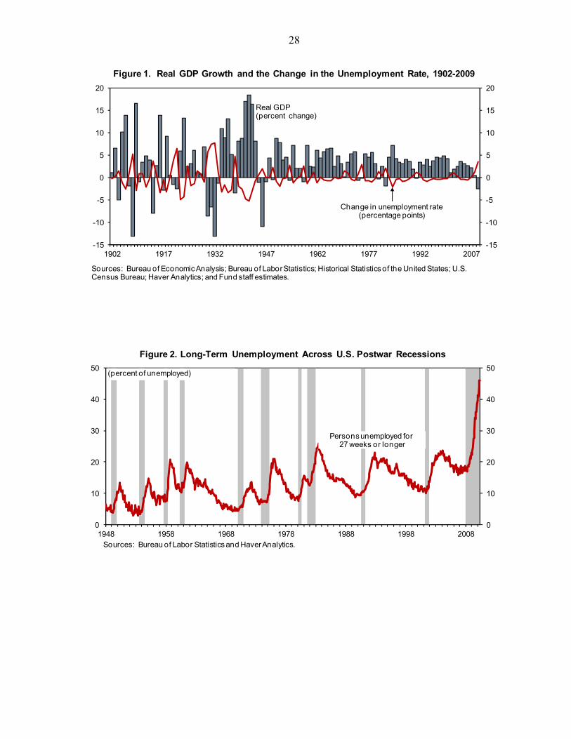
A. Introduction 1. The recent economic recession has had a severe impact on employment by historical standards and the recovery has not been “job rich” so far (Figure 1). The unemployment rate increased by over 5 percentage points since the onset of the crisis, reaching levels comparable to historic post-war records in the early-1980s recession. However, unlike past deep recessions and similarly to the previous two recessions, the unemployment rate has not improved much since the economic recovery started in the middle of 2009, and the duration of unemployment has actually increased (Figure 2). 2. These developments raise the specter of a “jobless recovery” going forward. Labor markets have changed significantly since the 1980s, with the past two recoveries being characterized by high productivity growth and little job creation. In addition, the current recession originated in a deep financial turmoil; a shock that historically has tended to have persistent impacts on job flows. These two facts suggest that jobs and unemployment may be slow to recover this time around as well. 3. This chapter argues that this recovery will be richer in jobs than the past two episodes if economic uncertainty declines significantly, although unemployment will probably remain elevated for a while. A comparison with past recessions shows that the recent episode produced a deeper labor adjustment than usual, including very weak labor cost growth. Econometric estimates show that the growth/(un)employment relationship has changed over time in the United States, with unemployment being more responsive to output changes during the recent crisis than in the previous 20 years. Shocks in financial conditions, relative labor costs, and economic uncertainty—measured here by stock market volatility—explain a good share of changes in the growth/(un)employment relationship, and suggest that rapid future employment gains will depend on a decisive reduction in uncertainty.
1 Prepared by Nicoletta Batini, Marcello Estevão, and Geoffrey Keim.
23
B. How Does this Recession Compare to Previous Ones? 4. The 2007 downturn followed a general pattern that places it in between the postwar recessions and the Great Depression (Figures 3–6). In particular:
• The current recession marked the largest postwar upswing in the unemployment rate and a similar upswing to that observed during the first phase (1930–1933) of the Great Depression. It also marked the largest postwar contraction in employment, but half the decline seen in the Great Depression.
• In the recent recession, more hours were lost relative to the ‘mild’ 1991 and 2001
downturns, but fewer hours (half) were lost relative to the Great Depression. The decline in total labor input followed the postwar trend with a 70:30 heads/hours split, contrary to the Great Depression during which more hours than persons were lost (with roughly a 40:60 heads/hours split).
• Unit labor costs have dropped more this time than in earlier downturns, although
less than in the Great Depression, a sign that wages are responding to the large flows into unemployment and to reductions in hiring rates. That bodes well for future employment growth vis-à-vis past recessions that faced weaker downward adjustments in labor costs.
5. As a result, the relationship between unemployment and growth was stronger during the recent recession than at any post-war recession (Figure 3). Increases in the rate of output growth have been associated consistently with a lower unemployment rate—with a ratio of 2½:1—and, statistically, this relationship has not shown structural breaks over 1900–2009 (in other words the ratio has not shifted permanently to higher or lower levels over time, hovering around its mean). However, this relationship has varied a lot in particular periods of time, and the current recession marks the second time in history following the Great Depression that the ratio shifted down drastically from its long-run average (implying a ratio of 1¾:1).2
A lower ratio suggests that—other things equal—each percentage point of growth above trend creates more jobs and vice versa.
2 These estimates are similar to Okun’s original estimates for the entire postwar era in the United States and are also close to Knotek’s (2007) updates of those estimates using data between 1948 Q2 and 2007 Q2.
24
C. How Will the Recovery be Like?
6. Turning to the recovery seen in the data, the initial evidence (2009 Q3-2010 Q1) points to similarities with the 1933–1934 recovery with respect to the behavior of unemployment and labor costs (Figures 3–6). In particular:
• Unemployment has continued to deteriorate in a way similar to the 1933–1934 recovery. To a lesser extent this also characterized other postwar recoveries, as unemployment is a lagging indicator of the cycle. Employment and the labor force however are adjusting more sluggishly this time around than during the Great Depression, likely reflecting differences in the type of shock behind each downturn.3
• Unit labor costs have declined sharply in 2009—also thanks to large increases in productivity—similarly to the Great Depression, but much less than in previous post-war recoveries.
7. To predict the path of recovery going forward, we focus on the relationship between employment and growth when economic uncertainty is high. In particular, we estimate a simple tri-variate SVAR relating changes in employment, real GDP growth, and stock market volatility (a proxy for economic uncertainty) using U.S. data from 1930 to 2009. As Figure 7 indicates, the highest-on-record spikes in volatility (in 1930 and 2008) coincide with lowest-on-record Okun’s ratios, suggesting that uncertainty about the economic environment is associated with more employment losses than during more certain times, given the same growth rate in real GDP. Impulse response functions from the SVAR (with shocks identified using the following Cholesky ordering: stock market volatility real GDP growthchanges in employment) reaffirm that an adverse shock to stock market volatility depresses employment growth, other things equal (Figure 8). 8. Our results show that the stronger-than-normal decline in employment per output lost between 2007 and 2008 reflected in great part mounting exceptional economic uncertainty at that time—as shown by the sharp increase in stock market volatility. With no recovery in sight and bad domestic and world macroeconomic news flowing in—an environment reminiscent of the 1930s, as acknowledged for example in Daly
3 As argued by many (e.g., Katz, 2010), the shock triggering the recent turmoil was different to the one in the Great Depression: (1) the recent shock has originated in the market for housing mortgages and thus hit the market for dwellings, generating a geographic lock-in effect that reduced mobility and job creation; (2) the shock penalized fast-growing areas; and finally (3) due to the specific type of credit crunch it generated, the recent shock proved particularly pernicious for start-ups in job-creating sectors.
25
and Hobijn (2010) and Krueger (2010)4
—firms opted for more firing and less hiring this time relative to previous recessions.
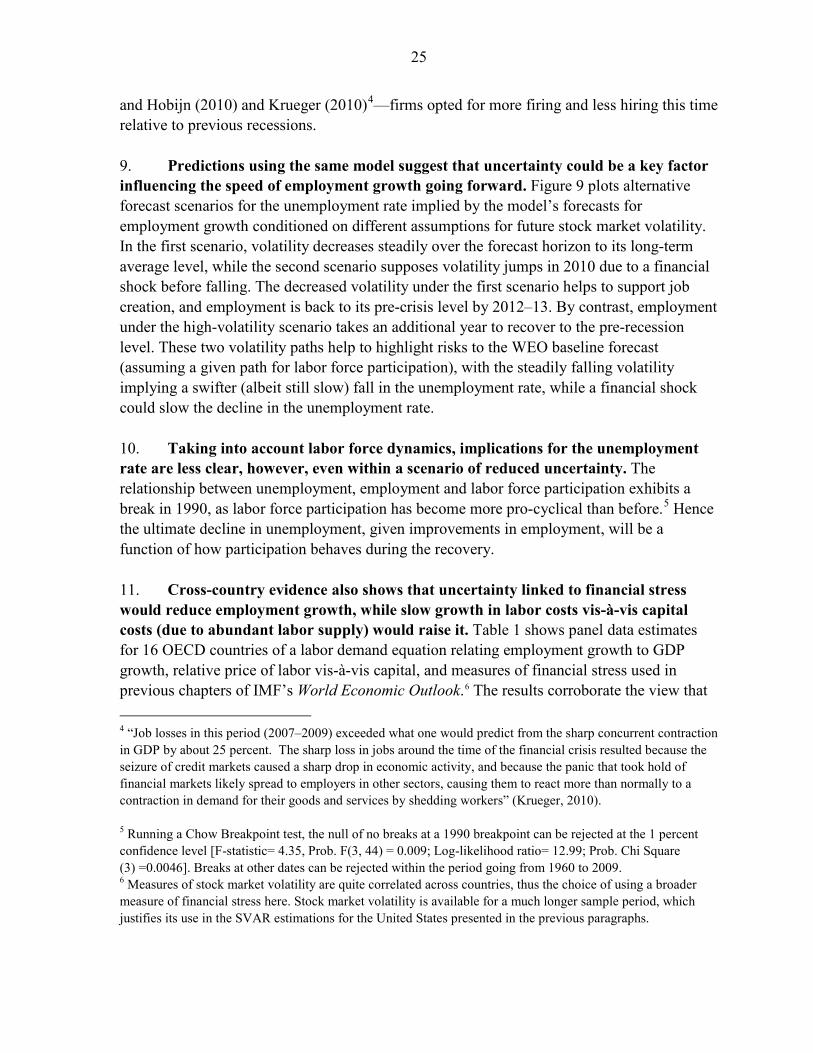
9. Predictions using the same model suggest that uncertainty could be a key factor influencing the speed of employment growth going forward. Figure 9 plots alternative forecast scenarios for the unemployment rate implied by the model’s forecasts for employment growth conditioned on different assumptions for future stock market volatility. In the first scenario, volatility decreases steadily over the forecast horizon to its long-term average level, while the second scenario supposes volatility jumps in 2010 due to a financial shock before falling. The decreased volatility under the first scenario helps to support job creation, and employment is back to its pre-crisis level by 2012–13. By contrast, employment under the high-volatility scenario takes an additional year to recover to the pre-recession level. These two volatility paths help to highlight risks to the WEO baseline forecast (assuming a given path for labor force participation), with the steadily falling volatility implying a swifter (albeit still slow) fall in the unemployment rate, while a financial shock could slow the decline in the unemployment rate. 10. Taking into account labor force dynamics, implications for the unemployment rate are less clear, however, even within a scenario of reduced uncertainty. The relationship between unemployment, employment and labor force participation exhibits a break in 1990, as labor force participation has become more pro-cyclical than before.5
Hence the ultimate decline in unemployment, given improvements in employment, will be a function of how participation behaves during the recovery.
11. Cross-country evidence also shows that uncertainty linked to financial stress would reduce employment growth, while slow growth in labor costs vis-à-vis capital costs (due to abundant labor supply) would raise it. Table 1 shows panel data estimates for 16 OECD countries of a labor demand equation relating employment growth to GDP growth, relative price of labor vis-à-vis capital, and measures of financial stress used in previous chapters of IMF’s World Economic Outlook.6
4 “Job losses in this period (2007–2009) exceeded what one would predict from the sharp concurrent contraction in GDP by about 25 percent. The sharp loss in jobs around the time of the financial crisis resulted because the seizure of credit markets caused a sharp drop in economic activity, and because the panic that took hold of financial markets likely spread to employers in other sectors, causing them to react more than normally to a contraction in demand for their goods and services by shedding workers” (Krueger, 2010).
The results corroborate the view that
5 Running a Chow Breakpoint test, the null of no breaks at a 1990 breakpoint can be rejected at the 1 percent confidence level [F-statistic= 4.35, Prob. F(3, 44) = 0.009; Log-likelihood ratio= 12.99; Prob. Chi Square (3) =0.0046]. Breaks at other dates can be rejected within the period going from 1960 to 2009. 6 Measures of stock market volatility are quite correlated across countries, thus the choice of using a broader measure of financial stress here. Stock market volatility is available for a much longer sample period, which justifies its use in the SVAR estimations for the United States presented in the previous paragraphs.
26
weak wage growth vis-à-vis the cost of capital and a reduction in financial stress would raise employment growth for a given GDP path. Estimates of a modified Okun’s Law equation—in which relative labor costs and measures of financial stress work as shifters in the relationship between GDP growth and the unemployment rate—show that unemployment would also decline faster for a given rate of GDP growth under weak wage growth and reduced financial stress.
D. Conclusions and Policy Implications
12. Overall, the analysis in this chapter points to a faster recovery in employment than observed in the “jobless recoveries” of the early 1990s and early 2000s. The basic reason for this conclusion can be put simply: as opposed to the other two episodes, employment has reacted very strongly to declines in production during the recession—probably because of the sharp increase in economic uncertainty. Going ahead, and also because of the large supply of available labor and the resulting sluggish labor costs, there are equilibrating pressures to hire more people for a given unit of production than during past shallow recessions. 13. However, some specific factors may dampen the rebound in employment, justifying additional policy support to job creation. The current episode has seen a surge in involuntary part-time employment—implying hours may grow ahead of “bodies” in the upturn—and ongoing economic shocks (more recently from Europe) are keeping uncertainty high. Tax incentives for net hiring could nudge firms to contract more labor for each unit of output being produced. Indeed, as discussed in Katz (2010), evidence for the United States suggests that firms respond to short-run reduction in marginal wage costs by moderately expanding employment (e.g., Card, 1990). Other evidence suggests that a net job creation tax credit would be an effective way to raise employment (Bartik and Bishop, 2009, and Congressional Budget Office, 2010). Estevão (2007) shows that subsidies to direct hiring by the private sector have been the best alternative among a set of active labor market policies to raise employment rates sustainably across a panel of OECD countries. To minimize economic distortions, subsidies should be temporary, though, and be unwound once unemployment rates get closer to structural levels. In addition, given the fiscal situation in the United States, any increase in spending in this area should be offset by a reduction in outlays in other areas or an increase in fiscal revenue.
27
(1) (2)Change in the number of
workersChange in unemployment
rate
Real GDP growth 0.526*** -0.449***(0.0492) (0.0328)
Hourly wage inflation - capital inflation differential -0.134*** 0.0375***(0.0225) (0.0141)
Lending rate 0.102** 0.00254(0.0450) (0.0295)
Financial stress index -0.0877 0.0356(0.0568) (0.0358)
Financial stress index, lagged one year -0.107* 0.0382(0.0594) (0.0374)
Financial stress index, lagged two years -0.143*** 0.0718**(0.0488) (0.0302)
Constant -2.619*** 1.735***(0.800) (0.486)
Dummy variables for countries Yes YesDummy variables for years Yes Yes
Number of observations 233 223R-squared 0.751 0.762
Table 1. Estimating Labor Demand and Okun's Law for a Panel of Countries
Notes: Standard errors are shown in parentheses. ***, **, and * denote significance at the 1 percent, 5 percent, and 10 percent levels, respectively. The dependent variable in equation (1) is the annual percent change in the number of workers, and in equation (2), the dependent variable is the first difference of the unemployment rate. The regressors included the percent change in real GDP, the difference between the hourly wage inflation rate (hourly wages were computed as the aggregate wage bill divided by aggregate hours) minus the inflation rate on capital goods (capital goods prices were measured as the implicit deflator on gross fixed capital formation), the bank lending rate, and a financial stress index, which is a weighted average of banking-related financial indicators, securities-market indicators, and exchange rate volatility (a higher value for index indicates increased stress in financial markets). Each equation also included country dummy variables to capture country fixed effects as well as year dummies. The sample included 11 advanced economies over 1983-2004.
28
Figure 1. Real GDP Growth and the Change in the Unemployment Rate, 1902-2009
Sources: Bureau of Economic Analysis; Bureau of Labor Statistics; Historical Statistics of the United States; U.S. Census Bureau; Haver Analytics; and Fund staff estimates.
-15
-10
-5
0
5
10
15
20
-15
-10
-5
0
5
10
15
20
1902 1917 1932 1947 1962 1977 1992 2007
Real GDP(percent change)
Change in unemployment rate(percentage points)
Figure 2. Long-Term Unemployment Across U.S. Postwar Recessions
Sources: Bureau of Labor Statistics and Haver Analytics.
0
10
20
30
40
50
0
10
20
30
40
50
1948 1958 1968 1978 1988 1998 2008
(percent of unemployed)
Persons unemployed for 27 weeks or longer
29
Figure 3. Rolling Okun's Law Coefficients and Growth Compatible with Stable Unemployment, 1915-2009
Sources: Bureau of Economic Analysis; Bureau of Labor Statistics; Historical Statistics of the United States; U.S. Census Bureau; and Fund staff estimates.
-0.8
-0.6
-0.4
-0.2
0.0
-2
0
2
4
6
1915 1930 1945 1960 1975 1990 2005
GDP growth consistent withstable unemployment (percent; left)
Coefficients from Rolling Okun's Law Regressions (right)
30
Figure 4. Comparing the Steep Recessions and Job-Rich Recoveries
Sources: Bureau of Economic Analysis, Bureau of Labor Statistics, and Fund staff estimates.
-5
0
5
10
15GDP Decline
Employment Decline
Hours Decline
Change in Unemployment Rate
Change in Labor Force Participation Rate
Unit labor costs
1957
1973
1981
2007
-15
-10
-5
0
5GDP Decline
Employment Decline
Hours Decline
Change in Unemployment Rate
Change in Labor Force Participation Rate
Unit labor costs
1958
1975
1982
2009
Contractions (Peak to Trough)
Recoveries (Trough to Three Quarters Later)
31
Figure 5. Comparing the Most Recent Recessions and Jobless Recoveries
-4
0
4
8GDP Decline
Employment Decline
Hours Decline
Change in Unemployment Rate
Change in Labor Force Participation Rate
Unit labor costs
1990
2001
2007
-6
-3
0
3
6GDP Decline
Employment Decline
Hours Decline
Change in Unemployment Rate
Change in Labor Force Participation Rate
Unit labor costs
1991
2001
2009
* Unemployment is scaled by a factor of 10.Sources: Bureau of Economic Analysis, Bureau of Labor Statistics, and Fund staff estimates.
Contractions (Peak to Trough)
Recoveries (Trough to Three Quarters Later)
32
Figure 6. Comparing the Great Depression and the Great Recession
Source: Bureau of Economic Analysis; Bureau of Labor Statistics; Kendrick (1961); Haver Analytics; and Fund staff estimates.
-30
-15
0
15
30GDP Decline
Employment Decline
Hours Decline
Change in Unemployment Rate
Change in Labor Force Participation Rate
Unit labor costs
1929
2007
-12
-8
-4
0
4GDP Decline
Employment Decline
Hours Decline
Change in Unemployment Rate
Change in Labor Force Participation Rate
Unit labor costs
1933-4
2009
Contractions (Peak to Trough)
Recoveries (1933-34 and 2009Q2-2010Q1)
33
Figure 7. Stock Market Volatility versus Rolling Okun's Law Coefficients
Sources: Bloomberg, LP and Fund staff estimates.
-0.8
-0.6
-0.4
-0.2
0.0
0
1
2
3
4
1928 1943 1958 1973 1988 2003
Stock market volatility
Coefficients from Rolling Okun's Law Regressions (right)
34
-0.2
0.0
0.2
0.4
0.6
-0.2
0.0
0.2
0.4
0.6
1 2 3 4 5 6 7 8 9 10
Figure 8. Impulse Responses from a Tri-Variate SVAR
Sources: Bureau of Economic Analysis; Bureau of Labor Statistics; Historical Statistics of the United States; U.S. Census Bureau; Bloomberg, LP; Haver Analytics; and Fund staff estimates.
-2
-1
0
1
2
-2
-1
0
1
2
1 2 3 4 5 6 7 8 9 10
+/- 2 StandardErrors
-4
-2
0
2
4
6
-4
-2
0
2
4
6
1 2 3 4 5 6 7 8 9 10
Response of employment growth to a one standard deviation shock to stock market volatility.
Response of real GDP growth to a one standarddeviation shock to stock market volatility
Response of stock market volatility to a one standard deviation shock to stock market volatility.
35
Figure 9. Unemployment Scenarios
Sources: Bureau of Labor Statistics; Bloomberg, LP; Haver Analytics; and Fund staff estimates.
0
1
2
3
0
1
2
3
2000 2002 2004 2006 2008 2010 2012 2014
(standard deviation of daily stock market returns)
Scenariowith Shock and High Volatility
Scenariowith FallingVolatility
3
6
9
12
3
6
9
12
2000 2002 2004 2006 2008 2010 2012 2014
(percent)
Scenariowith Shock and High Volatility
Scenariowith FallingVolatility
WEOBaseline
Unemployment Rate Forecasts
Financial Volatility Scenarios
AverageVolatility
1929-2006
36
REFERENCES
Bartik, Timothy, and John Bishop, 2009, “The Job Creation Tax Credit: Dismal Employment Projections Call for Quick, Efficient, and Effective Response,” EPI Briefing Paper #248.
Card, David, 1990, “Unexpected Inflation, Real Wages, and Employment Determination in
Union Contracts,” American Economic Review, 79, September. Congressional Budget Office, 2010, Policies for Increasing Economic Growth and
Employment in 2010 and 2011, January. Daly, Mary and Bart Hobijn (2010), “Okun’s Law and the Unemployment Surprise of 2009,”
FRBSF Economic Letter, 2010-07, Federal Reserve Bank of San Francisco, March. Estevão, Marcello, 2007, “Labor Policies to Raise Employment,” Staff Papers, Vol. 54, No.
1, pp. 113–138, March. Katz, Lawrence, 2010, Unemployment in the Great Recession: Structural Problems and
Policy Responses, Testimony for the Joint Economic Committee
, U.S. Congress, February.
Knotek, Edward S., II, 2007, “How Useful Is the Okun’s Law?” Economic Review, Federal Reserve Bank of Kansas City, fourth quarter, pp. 73–103.
Krueger, Alan, 2010, Statement before the Joint Economic Committee, U.S. Department of
Treasury, May 5. Okun, Arthur, 1962, “Potential GNP: Its Measurement and Significance,” Proceedings of the
Business and Economics Statistics Section, American Statistical Association, pp. 98–104.
37
IV. THE FINANCING OF U.S. FEDERAL BUDGET DEFICITS1
This chapter examines the potential effect of prospective increases in U.S. federal government debt on long-term bond yields. We present estimates of medium-term demand for U.S. Treasury debt and examine the portfolio adjustments that would be implied by high debt supply. We also investigate the implications of high public deficits for U.S. saving and investment flows using an econometric model. Based on standard empirical estimates of the impact of debt on interest rates, our results suggest that the increase in debt alone could add 50 to 150 basis points to the longer-term borrowing costs of the U.S. federal government.
A. Introduction
1. Who will finance the U.S. federal deficit in the medium term? The publicly-held debt of the federal government is expected to increase to 64 percent of GDP in 2010 from 36 percent in 2007. The federal budget deficit is expected to continue rising in the medium term on current policy proposals, which would bring the ratio of federal debt to GDP to levels not seen since the 1950s—on staff’s economic projections, to about 80 percent of GDP by 2015. Although the demand for debt has been brisk recently, the salient question is who will finance the future debt and at what cost once safe haven considerations subside.
B. Post-Crisis Financing Patterns
2. The post-crisis period has seen an increase in domestic holdings of Treasury debt. While domestic residents have historically accounted for the dominant share of holdings, the decade leading up to the crisis saw an increasing share of foreign purchases, in particular from emerging markets. In a reversal of this trend, about half of the net debt issuance in 2008–09 was purchased by U.S. residents, in particular the financial system in 2008, and households, nonprofits, and hedge funds in 2009.
1 Prepared by Oya Celasun and Martin Sommer.
U.S. Households
1/14%
U.S. Financial Sector 2/
33%
Federal Reserve
1%
China16%
Money Centers 3/
8%
Japan7%
Other21%
Net Purchases of U.S. Federal Publicly Held Debt in 2008–09
Sources: U.S. Department of the Treasury, Treasury International Capital System; Board of Governors of the Federal Reserve System, Flow of Funds Accounts; and Fund staff estimates.1/ Includes hedge funds and nonprofits.2/ Banks, Mutual Funds, Pension Funds, Insurers.3/ Barbados, the Bahamas, Bermuda, Cayman Islands, Netherlands Antilles, Panama, Hong Kong, Ireland, Luxembourg, Switzerland, and United Kingdom.
38
3. Going forward, foreign demand is unlikely to keep up with the supply of debt, implying that domestic residents will need to absorb an increasing share of debt issuance. Foreign purchases of U.S. Treasury securities would likely be determined largely by the prospective purchasers’ external surpluses, in particular official reserve accumulation, and motives to stabilize currencies against the U.S. dollar versus other currencies. Given limits on sustained expansions of foreign demand, domestic holdings of Treasury securities would have to increase. Among domestic holders, households and banks currently have the largest amounts of total gross financial assets and therefore the largest capacity to purchase federal debt securities, followed by pension funds and insurance companies. Households could potentially absorb further purchases given the likely increase in their saving rate, although a further portfolio allocation by the U.S. financial sector toward Treasury debt is uncertain against the ongoing deleveraging of banks and improving prospects for returns on private assets.
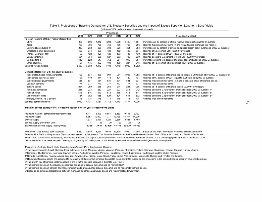
C. Baseline Projections of Demand for Treasury Debt 4. The future supply of debt is likely to exceed overall ex-ante demand by a significant margin. We project hypothetical demand paths on the basis of projections of domestic and foreign financial assets and other macroeconomic quanta (using World Economic Outlook projections of GDP, official reserves, external current and capital accounts) and assuming a return to pre-crisis asset allocation patterns (Table 1). In particular, we assume the following baseline demand paths for foreign residents during 2010–15:
• China continues to purchase Treasuries at a rate of 36 percent of its official reserve accumulation (close to the average ratio of purchases to reserve accumulation in 2000–07),
• Oil and other commodity exporters bring their purchases (as shares of current account surpluses or foreign asset purchases) to their 2000–07 averages by 2015,
• Other countries’ holdings return to 2000–07 averages as shares of GDP.
Under these conservative assumptions, foreign holdings would increase by three percent of GDP over the period 2010–15, while the gap between overall projected debt issuance and foreign holdings would increase by about 23 percent of GDP by 2015. At the same time, ex-
China: Current Account, International Reserves, and U.S. Treasury Holdings
Sources: U.S. Department of the Treasury, Treasury International Capital System; Haver Analytics; and IMF, World Economic Outlook.
0
100
200
300
400
500
600
700
800
0
100
200
300
400
500
600
700
800
2000 2005 2010 2015
Current Account
Change in Holdings
Change in Reserve Assets
(billions of dollars)
39
ante demand from domestic residents could decline by about 6 percent of GDP under the following assumptions: • The Federal Reserve and state and local governments do not increase their
nominal holdings (given the plan to gradually reduce the size of the Fed’s balance sheet and ongoing retrenchment by state and local governments),1
• Pension funds, insurers, and banks reduce their holdings to 2000–07 average shares of financial assets on the normalization of business conditions and risk appetite.
• Households keep their holdings at their current share of financial assets, which is somewhat higher than 2000–07 averages, but possibly sustainable on increased risk aversion after the wealth losses during the crisis. Household financial assets would rise in line with the staff’s projection of the personal saving rate.
Putting these demand projections together would imply 29 percent of GDP in “excess supply” of Treasury securities. 5. Higher real interest rates would likely be needed to encourage purchases of the future debt issuance in excess of the hypothetical path of demand. Assuming a yield impact of 2–5 basis points for each additional percentage point of GDP in excess debt supply would suggest an increase in yields in the range of 60–150 basis points in the medium term.2
D. A Model of Saving-Investment Flows
This effect would come on top of the increases due to rising short term interest rates (on the gradual exit of monetary policy from very low policy rates), and the normalization of the term premium excluding the debt effect. The staff’s baseline medium-term projection for the 10-year Treasury bond yield is about 6½ percent. An upside risk to this estimate could stem from a projected increase in closely-substitutable GSE-backed debt of roughly US$3.5 trillion between 2009 and 2015 on the basis of staff’s residential fixed investment forecast.
6. To supplement the above analysis of prospective demand based on portfolio choices of the key buyers of Treasury debt, staff has also estimated an econometric
1 The Fed’s holdings exceed seven percent of 2015 GDP—the historic average size of its balance sheet, implying that it could have an unchanged nominal portfolio of Treasury debt while shrinking its assets.
2 The empirical literature finds that a one percentage point in GDP increase in the public debt to GDP ratio increases long term bond yields by 2–5 basis points (see Laubach (2009) and Engen and Hubbard (2005). In this exercise, we apply this elasticity to a projected measure of excess supply of debt to take into account the sources of demand that would potentially offset the yield impact of increasing supply.
40
model of saving and investment flows using the national accounts data.3 This approach helps weigh the supply of savings by households and corporations against the demand for loanable funds by private and public sectors. The model can be used to test the frequently-discussed hypothesis that sluggish recovery in private demand will ease the upward pressures on long-term government bond yields. The econometric results suggest that while this hypothesis could hold in the near term, private investment will gradually pick up, diminishing the private sector surplus available for financing of the budget deficits. The dynamics of public deficits will then become critical for the path of interest rates and overall saving-investment balances:4
Near-term prospects
7. The general government net borrowing is projected by staff to drop from almost 11 percent of GDP in 2010 to 5½ percent in 2012 on expiring fiscal stimulus, diminishing slack in the economy, and initial steps toward fiscal consolidation planned by the authorities. Under the staff’s baseline assumption of the 10-year T-bond yield at 3½ percent in 2010 and 4¾ percent in 2011, the overall domestic saving-investment balance would have a tendency to remain broadly stable around current levels (-3½ percent of GDP), since strengthening private investment would be funded by reduced public dissaving and high household saving as consumers continue to rebuild their balance sheets.
Medium-term dynamics
8. In the absence of deeper fiscal consolidation in the medium term, however, the improvement in public saving will not last given pressures from population aging, health care spending, and higher debt. On current policies, the general government deficit is projected by staff to increase to 6 percent of GDP in 2015 and continue rising thereafter. Meanwhile, investment rates will return to historical norms. The econometric model suggests that interest rates materially lower than the staff’s medium-term baseline of around 6½ percent would imply a gradual deterioration of the saving-investment gap toward the levels seen during the bubble years, deepening the current account deficit and raising demand for external funding. However, such a scenario with lower interest rates could only materialize if availability of external saving was ample and investor appetite for government bonds relative to higher-yielding instruments such as equities remained strong—unlikely when the recovery is fully underway and the global economy is on a trajectory toward a more balanced growth.
3 The analytical framework will be presented in a forthcoming Working Paper.
4 The sum of private and public saving minus private and public investment.
41
E. Conclusions 9. In sum, analysis both on the basis of investor portfolios and saving-investment balances suggest that, on current policies, the sizeable projected increases in U.S. public debt will likely put upward pressure on government borrowing costs in the medium term. That said, the near-term developments are highly uncertain as U.S. Treasury debt continues to enjoy a safe haven status. Early agreement on longer-term fiscal consolidation plans—including through the dedicated Fiscal Commission—would help to solidify this position and avoid an unnecessary increase in long-term interest rates.
42
2009 2010 2011 2012 2013 2014 2015Foreign Holders of U.S. Treasury Securities China 895 1,006 1,112 1,203 1,308 1,420 1,561 Purchases at 36 percent of official reserve accumulation (2000-07 average) Japan 766 766 766 766 766 766 766 Holdings fixed in nominal terms (in line with a floating exchange rate regime) Commodity producers 1/ 239 258 280 302 326 351 383 Purchases at 20 percent of private and public foreign asset purchases (2003-07 average) Emerging market countries 2/ 429 374 399 429 462 498 531 Holdings at 5 percent of GDP (2000-07 average) France, Germany, Italy 99 123 126 129 133 136 139 Holdings at 1.4 percent of GDP (2000-07 average) Money centers 3/ 684 754 660 627 663 702 739 Holdings decline to 0.9 percent of world GDP (2000-07 average) Oil exporters 4/ 412 523 647 762 854 919 957 Purchases decline to 8 percent of current account balances (2003-07 average) Other countries 167 175 182 190 199 207 216 Holdings at 1 percent of other countries' GDP (2000-07 average)Subtotal, foreign holders 3,689 3,980 4,172 4,409 4,710 4,999 5,292
Domestic Holders of U.S. Treasury Securities Households, hedge funds, nonprofits 795 834 866 904 954 1,003 1,055 Holdings at 1.8 percent of financial assets (equal to 2009 level, above 2000-07 average) 5/ Nonfinancial business sector 105 110 114 119 124 129 134 Holdings at 0.7 percent of GDP (equal to 2009 level and 2000-07 average) State and local governments 531 531 531 531 531 531 531 Holdings fixed in nominal terms (remains a constant share of financial assets) Monetary authority 777 777 777 777 777 777 777 Holdings fixed in nominal terms Banking sector 207 250 258 265 274 284 296 Holdings at 1.5 percent of financial assets (2000-07 average) 6/ Insurance companies 236 233 230 227 223 218 212 Holdings decline to 2.7 percent of financial assets (2000-07 average) 7/ Pension funds 513 516 513 512 515 516 514 Holdings decline to 4.1 percent of financial assets (2000-07 average) 8/ Money market funds 727 702 665 629 594 551 502 Holdings decline to 2.8 percent of financial assets (2000-07 average) 8/ Brokers, dealers, ABS issuers 178 178 178 178 178 178 178 Holdings fixed in nominal termsSubtotal, domestic holders 4,069 4,131 4,131 4,142 4,170 4,187 4,200
Impact of excess supply of U.S. Treasury Securities on ten-year Treasury bond yields2,009 2,010 2011 2012 2013 2014 2015
Memo item: GSE-backed debt securities 8,360 8,540 8,954 9,549 10,300 11,090 11,756 Based on the WEO forecast of residential fixed investment 9/Sources: U.S. Treasury Department, Treasury International Capital System; The Board of Governors of the Federal Reserve System, Flow of Funds Accounts ; and Fund staff estimates.
5/ Household financial assets are assumed to increase to 430 percent of personal disposable income by 2015 (based on the projections in the selected issues paper on household savings).6/ The growth rate of banking sector assets is in line with the baseline scenario in the 2010 U.S. FSAP.7/ The financial assets of the insurance sector are assumed to grow at the same rate as nominal GDP.8/ The financial assets of pension and money market funds are assumed grow at the same rate as household financial assets.9/ Based on an estimated relationship between mortgage issuances and house prices and residential fixed investment.
Table 1. Projections of Baseline Demand for U.S. Treasury Securities and the Impact of Excess Supply on Long-term Bond Yields
Projection Method
(billions of U.S. dollars unless otherwise indicated)
1/ Argentina, Australia, Brazil, Chile, Colombia, New Zealand, Peru, South Africa, Uruguay. 2/ The Czech Republic, Egypt, Hungary, India, Indonesia, Korea, Malaysia, Mexico, Morocco, Pakistan, Philippines, Poland, Romania, Singapore, Taiwan, Thailand, Turkey, Ukraine. 3/ Barbados, The Bahamas, Bermuda, Cayman Islands, Netherlands Antilles, Panama, Hong Kong, Ireland, Luxembourg, Switzerland, and the United Kingdom. 4/ Canada, Kazakhstan, Norway, Algeria, Iran, Iraq, Kuwait, Libya, Nigeria, Qatar, Saudi Arabia, United Arab Emirates, Venezuela, Russia, and Trinidad and Tobago.
Projections
Notes: GDP, current account balances, reserve accumulation, and capital outflows projections are from the World Economic Outlook. A one percentage point increase in the debt-to-GDP ratio is assumed to increase ten year Treasury bond yields by 2-5 basis points, in line with estimates by Laubach (2008) and Engen and Hubbard (2005).
43
REFERENCES Engen, Eric, and R. Glenn Hubbard, 2004, “Federal Government Debt and Interest Rates,” in
NBER Macroeconomics Annual 2004, ed. by M. Gertler and K. Rogoff, (Cambridge, Massachusetts: MIT Press).
Laubach, Thomas, 2009, “New Evidence on the Interest Rate Effects of Budget Deficits and
Debt,” Journal of the European Economic Association, Vol. 7, No. 4, pp. 858–885.
44
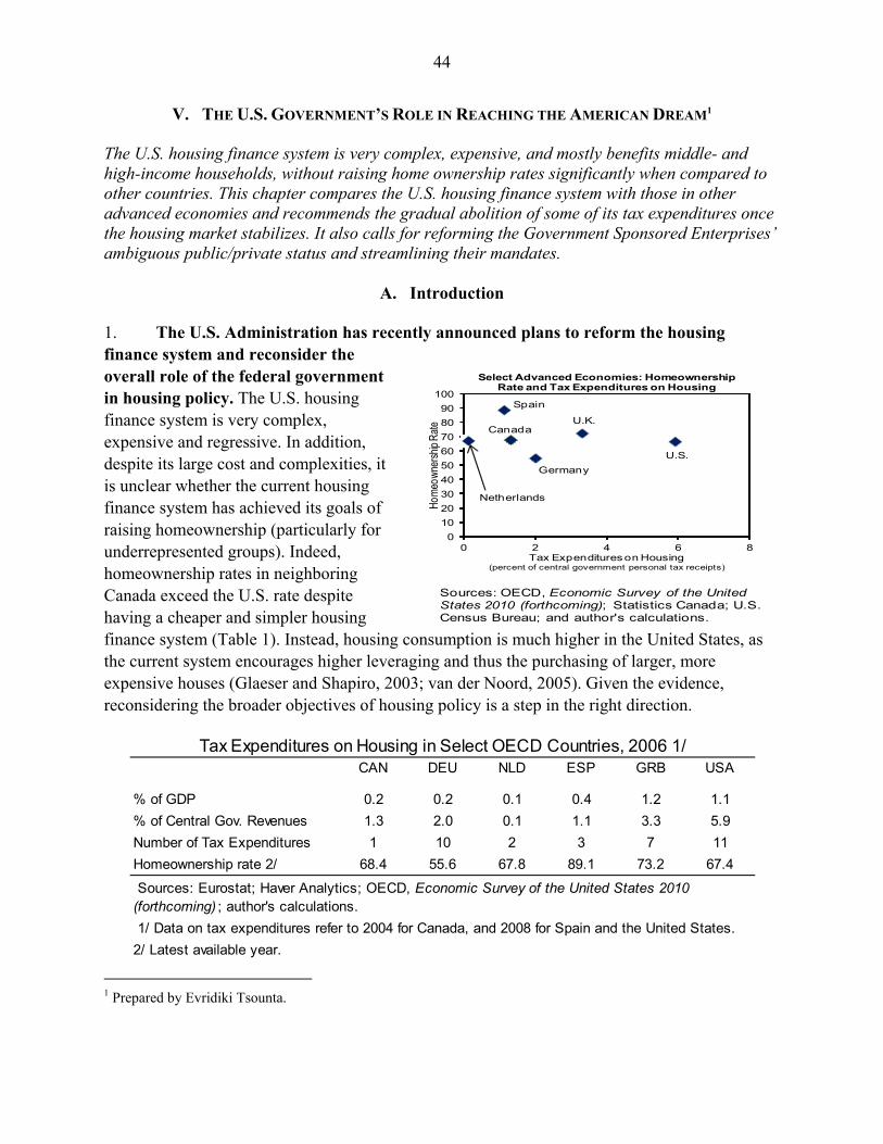
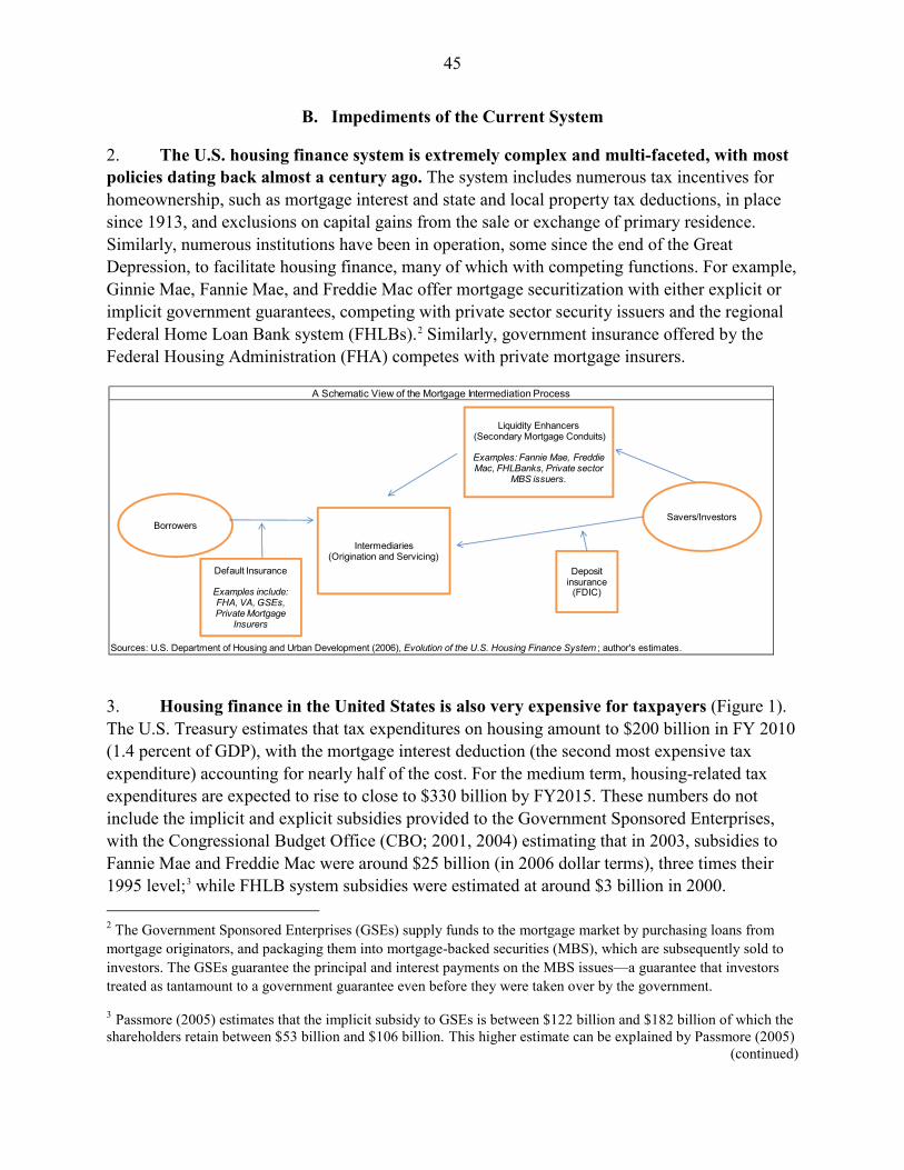
V. THE U.S. GOVERNMENT’S ROLE IN REACHING THE AMERICAN DREAM1
The U.S. housing finance system is very complex, expensive, and mostly benefits middle- and high-income households, without raising home ownership rates significantly when compared to other countries. This chapter compares the U.S. housing finance system with those in other advanced economies and recommends the gradual abolition of some of its tax expenditures once the housing market stabilizes. It also calls for reforming the Government Sponsored Enterprises’ ambiguous public/private status and streamlining their mandates.
A. Introduction
1. The U.S. Administration has recently announced plans to reform the housing finance system and reconsider the overall role of the federal government in housing policy. The U.S. housing finance system is very complex, expensive and regressive. In addition, despite its large cost and complexities, it is unclear whether the current housing finance system has achieved its goals of raising homeownership (particularly for underrepresented groups). Indeed, homeownership rates in neighboring Canada exceed the U.S. rate despite having a cheaper and simpler housing finance system (Table 1). Instead, housing consumption is much higher in the United States, as the current system encourages higher leveraging and thus the purchasing of larger, more expensive houses (Glaeser and Shapiro, 2003; van der Noord, 2005). Given the evidence, reconsidering the broader objectives of housing policy is a step in the right direction.
1 Prepared by Evridiki Tsounta.
CAN DEU NLD ESP GRB USA
% of GDP 0.2 0.2 0.1 0.4 1.2 1.1
% of Central Gov. Revenues 1.3 2.0 0.1 1.1 3.3 5.9
1/ Data on tax expenditures refer to 2004 for Canada, and 2008 for Spain and the United States.
2/ Latest available year.
Tax Expenditures on Housing in Select OECD Countries, 2006 1/
Sources: Eurostat; Haver Analytics; OECD, Economic Survey of the United States 2010 (forthcoming) ; author's calculations.
Sources: OECD, Economic Survey of the United States 2010 (forthcoming); Statistics Canada; U.S. Census Bureau; and author's calculations.
U.S.
U.K.Canada
Spain
Germany
0
10
20
30
40
50
60
70
80
90
100
0 2 4 6 8
Hom
eow
ners
hip R
ate
Tax Expenditures on Housing(percent of central government personal tax receipts)
Select Advanced Economies: Homeownership Rate and Tax Expenditures on Housing
Netherlands
45
B. Impediments of the Current System
2. The U.S. housing finance system is extremely complex and multi-faceted, with most policies dating back almost a century ago. The system includes numerous tax incentives for homeownership, such as mortgage interest and state and local property tax deductions, in place since 1913, and exclusions on capital gains from the sale or exchange of primary residence. Similarly, numerous institutions have been in operation, some since the end of the Great Depression, to facilitate housing finance, many of which with competing functions. For example, Ginnie Mae, Fannie Mae, and Freddie Mac offer mortgage securitization with either explicit or implicit government guarantees, competing with private sector security issuers and the regional Federal Home Loan Bank system (FHLBs).2
Similarly, government insurance offered by the Federal Housing Administration (FHA) competes with private mortgage insurers.
3. Housing finance in the United States is also very expensive for taxpayers (Figure 1). The U.S. Treasury estimates that tax expenditures on housing amount to $200 billion in FY 2010 (1.4 percent of GDP), with the mortgage interest deduction (the second most expensive tax expenditure) accounting for nearly half of the cost. For the medium term, housing-related tax expenditures are expected to rise to close to $330 billion by FY2015. These numbers do not include the implicit and explicit subsidies provided to the Government Sponsored Enterprises, with the Congressional Budget Office (CBO; 2001, 2004) estimating that in 2003, subsidies to Fannie Mae and Freddie Mac were around $25 billion (in 2006 dollar terms), three times their 1995 level;3
2 The Government Sponsored Enterprises (GSEs) supply funds to the mortgage market by purchasing loans from mortgage originators, and packaging them into mortgage-backed securities (MBS), which are subsequently sold to investors. The GSEs guarantee the principal and interest payments on the MBS issues—a guarantee that investors treated as tantamount to a government guarantee even before they were taken over by the government.
while FHLB system subsidies were estimated at around $3 billion in 2000.
3 Passmore (2005) estimates that the implicit subsidy to GSEs is between $122 billion and $182 billion of which the shareholders retain between $53 billion and $106 billion. This higher estimate can be explained by Passmore (2005)
(continued)
Sources: U.S. Department of Housing and Urban Development (2006), Evolution of the U.S. Housing Finance System ; author's estimates.
A Schematic View of the Mortgage Intermediation Process
Sources: OECD (2010), Economic Survey of the United States, forthcoming; U.S. Census Bureau; and author's calculations.
0
10
20
30
40
50
60
70
80
90
ESP GRC IRL BEL GBR AUS LUX CAN ITA USA FIN FRA AUT DNK SWE KOR DEU CHE
Homeownership Rates, latest available data(in percent)
4. These large fiscal costs end up benefiting middle- to high- income households (Figure 1). The majority of the tax measures are not well targeted, and they are largely enjoyed by upper income households that itemize deductions. The richer households benefit disproportionately since they face higher marginal income tax rates and usually have larger mortgages. However, their decision to buy a house is little influenced by government financial incentives, since on the margin they are not fiscally constrained on their decision to buy a house (Glaeser and Shapiro, 2003).
5. It is thus unclear whether subsidies affect homeownership rates, although they raise housing consumption. Data suggest that there is no strong correlation between homeownership rates and subsidies to housing, both across time and in cross country comparisons (Figure 1). In fact, U.S. tax expenditures on housing and homeownership rates have been negatively correlated in the last two decades, while homeownership rates are much higher in some countries (e.g., Australia, Canada, Spain) than in the United States, despite less generous subsidies and simpler housing finance systems; for instance, neither Canada nor Australia have a mortgage interest deduction. It appears on the other hand, that the mortgage interest deduction affects housing consumption (i.e., the size of the house) with Australian mortgages around 40 percent lower than the ones in the United States. Van den Noord (2005) shows that a tax system that favors homeownership through subsidies and tax deductions raises the equilibrium price of housing and price volatility, using a sample of euro area countries. In addition, Lehnert et al. (2008) find little evidence that GSEs lower interest rate spreads or raise homeownership.
C. Lessons from Other Countries
6. Experience from other countries indicates that considering a less complex and cheaper system for the United States is warranted. For example, other Anglo-Saxon countries such as Australia, Canada and the United Kingdom are enjoying higher homeownership rates considering the value embedded in all debt outstanding while the CBO only considers recent debt issuances during a given year.
47
than the United States, without having a mortgage interest deduction. Australia’s experience also indicates that public mortgage insurance is not necessary for a well-functioning housing finance system.4
Similarly, Canada’s explicit government guarantees on mortgage funding have shielded the system from the ambiguities related to the pre-crisis hybrid public/private status of the GSEs in the United States. In that respect, reforms to the GSE’s ambiguous public/private status, which proved unsustainable, could be considered, as well as streamlining their mandates and making explicit the guarantees on their business activities that provide public goods. Privatizing their retained portfolio, which bore little relation to the core bundling and guarantee businesses could also be considered.
7. Reforming tax incentives in housing finance has been successfully undertaken in many countries. The importance of subsidies to homeownership, notably of tax deductibility of interest payments, has decreased over time in many countries; for instance, the effective marginal tax rate at which mortgage interest tax relief can be claimed was reduced over time in Ireland from 47 percent to 20 percent and in Denmark from about 33.5 percent to 25.5 percent above a certain threshold, and has been progressively reduced in the United Kingdom over 12 years and completely eliminated in 2000, with minimal implications for the housing market and homeownership rates (Figure 1).5
8. In contrast, attempts thus far to reduce the generosity of the U.S. mortgage interest deduction have not borne fruit. In 2005, a bipartisan tax reform commission, proposed ending the mortgage interest deduction, but the plan stalled in Congress. In 2009, the Administration proposed cutting the deduction rate for itemized expenses for those making more than $250,000 to the rate paid by the middle class, but again it stalled in Congress; a similar proposal is pending again this year. Such reform would result in significant savings: the CBO (2009) recommended that by reducing the $1 million cap on the size of mortgage for which interest is deductible by $100,000 a year beginning in 2013 and ending at $500,000 in 2018, the Administration could generate $41.4 billion in additional revenues over 10 years. Alternatively, by changing the mortgage interest deduction to a 15 percent tax credit on mortgage interest for everyone with
4 The Australian Housing Loan Insurance Corporation (HLIC) was privatized in 1997, originally established to facilitate the development of an Australian secondary mortgage market. The privatization followed the recommendations of the Wallis Inquiry—a review of financial sector regulation undertaken to ensure that government policy would promote market outcomes (Australia, Ministry for Finance and Administration, 1997). The inquiry recommended that government guarantees be withdrawn from the HLIC to ensure that the mortgage market operated on competitively neutral terms. Following the privatization, homeownership rates were essentially unchanged. Now, the Australian mortgage market is made up of private insurers. 5 Beginning in 1983, the United Kingdom limited deductible interest on a maximum loan of £30,000—that became binding over time (Yelten, 2006). That limit was never raised, in spite of rising home prices, and the tax rate at which it was deductible was progressively phased down since 1993 from 25 percent to 10 percent before disappearing completely in 2000 (Gibb, Munro and Satsangi, 1999). In contrast, the corresponding ceiling for the United States is much more generous at $1 million plus home equity indebtedness of up to $100,000 with no upper limit on the tax rate.
48
mortgage amount below the declining limits in the aforementioned option, revenues would increase by $387.6 billion over 10 years. 9. The pace and timing of any adjustment need to bear in mind the state of the housing market. The disruptive experience in Sweden in the early 1990s and the favorable experience in the United Kingdom with gradual phasing out of interest relief for homeowners suggests that spreading out reforms of housing finance over time could avoid large disruptions to housing markets and minimize any adverse macro-financial implications. It is also important to choose a period when the housing market is in a relatively healthy state. For example, when Sweden first reduced the maximum deductible tax rate that could be applied to mortgage interest payments to 50 percent (from 80 percent) in 1985, the housing market was not hurt; indeed, real house prices experienced spectacular growth since the country was in the midst of strong economic growth. However, when the rate was subsequently reduced further to 30 percent in 1991—in the midst of one of Sweden’s worst recession—the housing market and economic activity tumbled (with nominal house prices declining by an average annual rate of 10¼ percent in 1992–93).
D. Conclusions and Policy Implications
10. The U.S. Administration is appropriately considering fundamental reforms to its housing finance system. The road to reform would be complicated given that most measures and institutions have been in place for almost a century. However, lessons could be learned from other countries that have successfully phased down government intervention in housing finance. In general, gradually moving away from the current complex, regressive and costly financing system would be desirable.
49
United States Canada
HomeownersExclusion of net imputed rental income √ √Deductibility of mortgage interest on owner-occupied homes √ ΧDeductibility of State and local property tax on owner-ocupied home √ ΧDeferral of income from instalment sales √ ΧCapital gains exclusion on home sales √ √Credit for homebuyer (temporary) √ √Exception of sales tax for purchase of resale homes Χ √
InvestorsExclusion of interest on rental housing bonds √ ΧExclusion of interest on owner occupied mortgage subsidy bonds √ ΧException from passibve loss rules for $25,000 of rental loss √ ΧCredit for low-income housing investments √ ΧAccelerated depreciation on rental housing (normal tax method) √ ΧDisccharge of mortgage indebtedness √ Χ
Public (Federal) FHA and VA CMHCPublic (state) Massachussettes ΧPrivate loan coverage 20-30% 90%
Ginnie Mae NHA MBSGSEs Χ√ √
GSEs Canada Mortgage Bonds √ √√ √
Sources: Finance Canada, personal contacts ; U.S. Office of Management and Budget (2010), Analytical Perspectives, Budget of the U.S. Government Fiscal Year 2011; and author's calculations.
Mortgage securitization with no government guarantee Corporate bonds issued by special facilities Corporate bonds issued by secondary market conduitsCorporate bonds issued by primary market lenders
Mortgage securitization with implicit government guarantee
Table 1. United States and Canada: Housing Finance
Tax Expenditures
Mortgage Insurance
Wholesale FundingMortgage securitization with explicit government guarantee
50
Figure 1. Housing Finance in the United States and Other OECD Countries
Sources: Australian Bureau of Statistics; Committee on the Budget, United States Senate (2008), Tax Expenditures: Compendium of Background Material on Individuals' Provisions; Haver Analytics;International Monetary Fund, World Economic Outlook; U.S. Census Bureau (1989), Historical Statistics: Colonial Times to 1970; U.S. Of f ice of Management and Budget (2010), Analytical Perspectives, Budget of the U.S. Government Fiscal Year 2011; Yelten (2006); and author's calculations.
40
45
50
55
60
65
70
75
1890 1940 1965 1975 1980 1985 1990 1995 2000 2005
U.S. Homeownership rate. 1890-2009(in percent)
0
0.2
0.4
0.6
0.8
1
1.2
1.4
1.6
1.8
2
1994 1997 2000 2003 2006 2009 2012 2015
Tax expenditures on Housing by Beneficiary(Fiscal Year, percent GDP)
Other tax expenditures to homeowners
Tax Expenditures to Investors
Mortgage Interest Deduction
0
5
10
15
20
25
30
35
40
45
50
Below $10
$10 to $20
$20 to $30
$30 to $40
$40 to $50
$50 to $75
$75 to $100
$100 to $200
$200 and over
Distribution by Income Class of the Mortgage Interest Tax Deduction, 2007(in percent)
(Thousands)
6062646668707274767880
1.0 1.2 1.4 1.6
Hom
e O
wne
rshi
p R
ate
(per
cent
)
Tax Expenditure on Housing (percent of GDP)
U.S. Home Ownership Rate and Tax Expenditures on Housing, 1994-2009
58
60
62
64
66
68
70
72
74
1971 1976 1981 1986 1991 1996 2001 2006
Homeownership Rates, 1971-2009
United States
Canada
Australia
0
5
10
15
20
25
30
35
40
45
50
45
55
65
75
85
95
1991 1995 1999 2002 2005
Maximum Applicable Income Tax Rate (right scale)
Homeownership Rate
Percent of Mortgages not Eligible for Deduction
United Kingdom: Mortgage Interest Deduction Eligibility, Applicable Tax Rate and Homeownership Rate
The U.S. homeownership rate remained essentially unchanged since the mid-1960s... ...despite rising subsidies, such as in mortgage
interest deductions...
...which are rather regressive......and are negative correlated with homeownership .
Australia and Canada, without mortgage deductions have higher homeownership rates that the United States...
...and the U.K. sucessfully eliminated its mortgage interest deduction.
51
REFERENCES
Australia, Ministry for Finance and Administration (1997), “Reform of the Australian Financial System,” Treasurer's Press Release No. 102, Canberra: Treasury.
Congressional Budget Office (CBO) (2001), Federal Subsidies and the Housing GSEs, Washington, DC: U.S. Government Printing Office.
-------- (2004), Updated Estimates of the Subsidies to the Housing GSEs, Washington, DC:
U.S. Government Printing Office. -------- (2009), Budget Options, Vol. 2, August.
Gibb, K., M. Munro and M. Satsangi (1999), Housing Finance in the UK: An Introduction, Palgrave Macmillan.
Glaeser, E.L. and J.M. Shapiro (2003), “The Benefits of the Home Mortgage Interest Deduction,” in Tax Policy and the Economy, Vol. 17, pp. 37–82, National Bureau of Economic Research.
Lehnert, A., W. Passmore and S.M. Sherlund (2008), “GSE’s, Mortgage Rates, and Secondary Market Activities, The Journal of Real Estate Finance and Economics, Vol. 36(3), pp. 343–63.
Passmore, W. (2005), “The GSE Implicit Subsidy and the Value of Government Ambiguity,” Real Estate Economics, Vol. 33.
Yelten, S. (2006), “House Prices In the Netherlands: Determinants, Concerns, and Considerations Related to Phasing Out the Tax Deductibility of Mortgage Interest Payments,” Kingdom of the Netherlands—Netherlands: Selected Issues, IMF Country Report No. 06/284, Washington, DC: International Monetary Fund.
Van den Noord, P. (2005), “Tax Incentives and House Price Volatility in the Euro Area: Theory and Evidence,” Économie Internationale, Vol. 101, pp. 29–45.
52
VI. THE U.S. FISCAL GAP: WHO WILL PAY AND HOW?1
This chapter quantifies the fiscal adjustment needed to stabilize debt/GDP over the very long run and also examines the generational imbalance (the difference in net taxes faced by current versus future generations). Both the fiscal and generational imbalances are large: we estimate an adjustment between 7 ¾ and 14 ½ percent of every future year’s GDP to restore sustainability and fiscal equity. A permanent cap on the growth of Medicare spending, along with the 2 ¾ percent of GDP adjustment advocated in the Staff Report, would eliminate 40 percent of the fiscal gap. The needed adjustment would rise if delayed.
A. Introduction 1. The United States is facing major fiscal and generational imbalances. The combination of high fiscal deficits, an aging population and rapid growth in government-provided healthcare benefits have put the fiscal accounts on an unsustainable path. Staff and Congressional Budget Office forecasts imply that U.S. debt will rise rapidly relative to GDP in the medium to long term (Figure 1).
B. Methodology 2. To measure the U.S. fiscal imbalance we compute the “fiscal gap”. Over a finite horizon, it measures the reduction in the deficit required so that the debt-to-GDP ratio in a particular year is the same as today. Over an infinite horizon, it measures the adjustment needed for the government to meet its intertemporal budget constraint, e.g., so that the present value of the excess of future expenditure and current liabilities over future receipts is zero. It has been argued that when fiscal pressures are concentrated in the long run, as in the United States, using the infinite horizon definition is preferable because finite horizon measures of the gap can underestimate the necessary adjustment (see Gokhale and Smetters, 2006). 3. To measure the U.S. generational imbalance we compute a set of generational accounts for all current and future U.S. generations. Generational accounts indicate the net present value amount that current and future generations are projected to pay to the government now and in the future. The accounts can be used to assess the fiscal burden current generations place on future generations, and thus offer a measure of the fiscal adjustments needed to make the fiscal structure generationally equitable (the Appendix offers details on the methodology used to compute the generational accounts).
1 Prepared by Nicoletta Batini, Giovanni Callegari and Julia Guerreiro. Laurence Kotlikoff served as a consultant on this project.
53
4. Two main fiscal scenarios are used (Figure 2):
• The staff’s baseline fiscal scenario (hereafter ‘Staff Scenario’), based on the IMF’s staff macroeconomic forecast (see Table 1).
• An alternative scenario (hereafter ‘Alternative Scenario’) based on the Congressional
Budget Office’s (CBO) June 2010 Alternative Long-Term Scenario. 5. Both the Staff and Alternative scenarios are based on CBO’s concept of “current policies”, in line with the 2010 CBO Alternative Long-Term Scenario. Both scenarios incorporate the budgetary impact of the Final Healthcare Legislation until 2020 as documented in CBO (2010d). Post 2020, the scenarios make identical assumptions about mandatory spending on health care, namely that several policies enacted in the Final Healthcare Legislation that would restrain growth in spending would not continue in effect (see CBO, 2010e). Both the Staff and Alternative Scenarios incorporate the limit beginning in 2015 on Medicare spending on a per capita basis, to a fixed growth rate, initially set at a mix of general inflation in the economy and inflation in the health sector (in line with CBO, 2010d). However, the scenarios do not incorporate the upper limit on Medicare spending to be set by the IPAB permanently at per capita gross domestic product growth plus one percentage point starting in 2018. Likewise, both scenarios assume that the extra revenues envisaged under a full enactment of the Final Healthcare Legislation will not increase as a share of GDP after 2020. These assumptions have a potentially large effect on the size of the fiscal gap because the full implementation of such policies—according to OMB estimates—could reduce the fiscal gap by some 2 to 3 percentage points of GDP. However, they reflect a view, incorporated in CBO’s Alternative Long-Term Scenario, that changes to the current law are likely to occur or that some provisions of law may be difficult to maintain for a long period. Finally, both scenarios assume that healthcare spending remains stable in terms of per capita GDP after 2083.
6. The main differences between the Staff and the Alternative Scenarios are: (1) the Staff Scenario is based on lower growth and higher real interest rate assumptions between 2011–2015, reflecting the staff’s assumption of a permanent output loss after the crisis, and higher debt financing costs in the medium term; (2) the Staff Scenario assumes, in line with the Administration’s FY2011 budget, that the tax cuts enacted in the Economic Growth and Tax Relief Reconciliation Act of 2001 (EGTRRA), the Jobs and Growth Tax Relief Reconciliation Act of 2003 (JGTRRA) expire only for higher income households, and an extension of some of the tax relief provisions in the American Recovery and Reinvestment Act of 2009 (ARRA, Public Law 111-5) in line with the Administration’s FY2011 budget (the CBO alternative scenario assumes that the EGTRRA and JGTRRA are made permanent).
54
C. Results 7. The U.S. fiscal gap associated with today’s federal fiscal policy is huge for plausible discount rates (Table 2). Using the same discount rate (3 percent) used by the Trustees of the Social Security Administration (2009) in their own Social Security-specific fiscal gap analysis and by CBO (2010e), and the infinite horizon definition, the U.S. fiscal gap is about 14 percent of the present discounted value of U.S. GDP under the Staff’s Scenario. This implies that closing the fiscal gap requires a permanent annual fiscal adjustment equal to about 14 percent of U.S. GDP, that is to say that fiscal revenues and spending would need to change so that the primary balance predicted under that scenario improves by this amount every year into the indefinite future starting next year.2
Using the Alternative Scenario the fiscal gap increases to about 14½ percent of the present discounted value of GDP (owing to the assumption that tax cuts are made permanent).
8. The fiscal gap under a finite horizon definition, or a larger discount factor, is smaller (but still sizeable) (Tables 2 and 3). Using a 6 percent discount factor reduces the gap to 7¾ to 8½ percent of GDP.3 Targeting a return to the 2008 federal debt-to-GDP ratio by 2083 under the Alternative Scenario, for example, implies a fiscal gap of about 8½ percent of GDP.4
9. The main drivers of the fiscal gap are rising healthcare costs that under current law will boost mandatory spending to above 18 percent of GDP by 2050.5
Since the federal government has historically collected about 18.4 percent of GDP in tax revenues, this means that mandatory programs may absorb all federal revenues sometime around 2050, or as early as 2026 when the cost of servicing the debt is added. As a result, future entitlement reforms will be necessary to restore fiscal sustainability.
2 Technically, the ratio of the fiscal gap to the present discounted value of GDP shows how much of the gap adjustment can be apportioned to each year from now to infinity to ensure intertemporal solvency. 3 A higher discount rate indicates a low propensity to save now for future consumption, a form of spending impatience, implying that the current government attaches more weight to the welfare of current generations relative to the welfare of future generations. In this sense, the discount rate is different than the cost of financing government borrowing that is embedded in our two fiscal scenarios. In general, the higher the discount rate, the lower the present value of future cash flows—hence a lower fiscal gap. 4 This number is close to the figure (8¾ percent of GDP) derived by CBO (2010) using a 75-year-horizon. The small difference is due to the fact that the CBO calculations employ a variable real interest rate, while Fund staff uses a constant rate throughout. 5 Population aging is also an important driver but far less than the increase in healthcare costs; the increase in healthcare costs is in turn due to various factors, the more important of which is technological change. This factor is summarized in CBO’s “excess growth component” of health-care costs growth (see CBO, 2010).
55
10. The gap remains large even excluding the adverse fiscal effects from the crisis (Table 2). The crisis had a sizeable fiscal impact in deficit terms over 2008, 2009, and 2010. However, its impact is ‘modest when compared to the wave of future liabilities.6
11. The U.S. generational imbalance is also large. Applying “generational accounting” to U.S. data indicates that—under the Staff’s Scenario—unless currently living Americans pay more in net taxes or unless government spending on current generations is curtailed, future Americans will face net tax rates that are about 14½–16½ percentage points of the present discounted value of labor income higher than those facing current newborn Americans under our scenarios (See Table 4).7
12. Implementing a fiscal adjustment equivalent to 2 ¾ percent of GDP by 2015 as suggested in the Staff Report reduces considerably the fiscal gap (Table 5). Were the adjustment to be followed by a permanent cap on Medicare spending, as mandated under the Final Healthcare Legislation to the Independent Payment Advisory Board and entailing the adoption of a rule that controls the excess growth in healthcare costs from Medicare, this would eliminate 40 percent of the fiscal gap, going a long way in eliminating the country’s fiscal problems (Table 5).
13. The fiscal adjustment would entail significant adjustments in taxes and/or transfers. Under the Staff’s Scenario, for example, the federal government can restore fiscal balance, conditional on the 2¾ percent of GDP fiscal adjustment by 2015 and the cap on Medicare spending by raising all taxes and cutting all transfer payments from 2015 onwards by 18 percent (Table 6). This would raise the U.S. tax revenue-to-GDP ratio to just below Germany’s, while still leaving it below that of many other advanced G-20 countries (Figure 3). A 5- or 10-year delay in the implementation of such residual fiscal adjustment would imply the need of ever larger additional increases in taxes/cut in transfers, equal to 19 and 21 percent, respectively (see Table 6).
6 To assess the impact of the crisis, individual and capital income taxes are set at the pre-crisis GDP ratio level for 2009–11. Unemployment compensation and food stamps are set at the pre-crisis GDP ratio for 2009–14. Discretionary spending is reduced in order to exclude fiscal stimulus and above-the line financial sector support above the line. Relatedly, IMF Staff Position Note SPN 2009/13 calculates that the PV of the impact of the financial crisis in only 7½ percent of the PV of age-related fiscal costs. 7 As Table 4 indicates, projected transfers to current generations, particularly health care, have become so substantial as to drive the lifetime net tax payment of current generations negative.
56
D. Conclusions 14. Sizeable fiscal actions would be needed to close the U.S. fiscal and generational imbalances. Under current policies, the United States federal debt is projected to grow rapidly due to a combination of large budget deficits before and during the crisis, as well as, over the medium term, demographic factors and healthcare inflation. As part of the medium term adjustment, the authorities would need to raise taxes and/or cut transfers substantially to avoid an undesirable escalation of the debt-to-GDP ratio. The longer the wait, the larger the necessary adjustment will be and the greater the burden on future generations.
Table 2. U.S. Fiscal Imbalance in Terms of the Present Discounted Value of GDP
Discount Rate 3% 6% Staff Scenario 13.9 8.3
No Financial Crisis 13.8 7.7
Alternative Scenario 14.4 8.6
No Financial Crisis 14.3 8.0
Source: Authors calculations. Note: All calculations are obtained taking present values as of fiscal-year-end 2009, and interpreting the policies in the FY 2010 Federal Budget as “current policies”.
58
Table 3. Fiscal Imbalance in Terms of the Present Discounted Value of GDP,
3 Percent Discount Rate
Staff
Scenario Alternative
Scenario
Finite horizon - Target: 2008 level of debt (44 percent of GDP)
25-year fiscal gap (2009-2033) 4.4 4.6 50-year fiscal gap (2009-2058) 6.1 6.7 75-year fiscal gap (2009-2083) 7.7 8.4
Memo: Infinite horizon - Full repayment of debt 13.9 14.4
Table 4. Lifetime Net Taxes as a Share of Present Value of Labor Income Under Different Scenarios, 3% Discount Rate Staff Scenario Alternative Scenario Zero year old -2.0 -2.0
Future new born 13.4 14.2
Table 5. Impact on Fiscal Gap (as % of PDV of GDP) of Fiscal Adjustment by 2015 and of Cap on Medicare
Discount Rate Staff Scenario 3% 6%
2 3/4 of GDP Adjustment on Taxes over 2010–15 11.2 5.9 2 3/4 of GDP Adjustment on Taxes over 2010–15 AND Medicare Cap 6.9 4.5 2 3/4 of GDP Adjustment on Taxes and 10.5 Transfers over 2010–15 5.7 2 3/4 of GDP Adjustment on Taxes and 6.5 Transfers over 2010–15 AND Medicare Cap 4.3
Table 6: Additional Percent Increase in Taxes and/or Cut in Transfers Necessary to Close the Fiscal Gap if Adjustment Starts In:1’ 3
2015 2020 2030 Raising taxes only on:
Individual income 60 63 70 Payroll income 119 128 146 Individual and payroll income 40 42 47
Raising all taxes2 34 36 41
2015 2020 2030
Raising all taxes and cutting transfers only on:
Social security 27 28 32 Medicare 25 27 29 Medicaid 28 30 33 Medicare and Medicaid 22 23 25
Raising all taxes and cutting all transfers 18 19 21
1 Applied to both current and future generations.
2 Including all other taxes like capital income, excise etc. 3 Under Staff Scenario, after 2¾ of GDP fiscal adjustment by 2015 and Medicare cap, to close fiscal gap computed using a 3 percent discount rate.
60
Figure 1. U.S. Debt in Percent of GDP (1930–2083) /1
Figure 2. U.S. Federal Fiscal Overall (solid) and Primary Deficit (dotted)
in Percent of GDP (1980–2083)
0
200
400
600
800
1,000
1,200
1,40019
30
1940
1950
1960
1970
1980
1990
2000
2010
2020
2030
2040
2050
2060
2070
2080
Alternative Scenario
Staf fScenario
-90
-80
-70
-60
-50
-40
-30
-20
-10
0
10
20
1930
1940
1950
1960
1970
1980
1990
2000
2010
2020
2030
2040
2050
2060
2070
2080
AlternativeScenario
Staf f Scenario
PB AlternativePB Staf f
61
Figure 3. Total Revenues and Tax Revenues in Percent of GDP—Advanced G-20 Countries
Sources: IMF, Government Finance Statistics, 2009; International Financial Statistics; and World Economic Outlook. 1/ 2006 data for Japan and 2007 data for all other countries.
0.0
10.0
20.0
30.0
40.0
50.0
60.0
Italy Australia Canada United Kingdom
France Germany United States
Japan Korea
Tax Revenues
Total revenues
62
REFERENCES
Auerbach, A. J., Gokhale, J. and L. J. Kotlikoff, 1991. Generational Accounting: A Meaningful Alternative to Deficit Accounting, NBER Chapters in Tax Policy and the Economy, Volume 5, pages 55-110 National Bureau of Economic Research, Inc.
CBO (2009a), “An Analysis of the President's Budgetary Proposals for Fiscal Year 2010”,
Congressional Budget Office, June 2009. CBO (2009b), “Economic and Budget Issue Brief”, Congressional Budget Office, December
2009. CBO (2010a), “The Budget and Economic Outlook: Fiscal Years 2010 to 2020”,
Congressional Budget Office, January 2010. CBO (2010b), “Budget and Economic Outlook: Historical Budget Data”, Congressional
Budget Office, January 2010. CBO (2010c), “An Analysis of the President's Budgetary Proposals for Fiscal Year 2011”,
Congressional Budget Office, March 2010. CBO (2010d), “H.R. 4872, Reconciliation Act of 2010 (Final Health Care Legislation)”,
Congressional Budget Office, March 2010. CBO (2010e), “The Long Term Budget Outlook”, Congressional Budget Office, June 2010. Gokhale, J. B. R. Page and J. Sturrock (1999), “Generational Accounts for the United States:
An Update”, in Generational Accounting Around the World, A. J. Auerbach, L. J. Kotlikoff and W. Leibfritz (eds).
Gokhale, J. and K. Smetters (2003). “Fiscal and Generational Imbalances: New Budget
Measures for New Budget Priorities”, AEI Press, Washington, D.C. IMF (2009), “The State of Public Finances Cross-Country Fiscal Monitor: November 2009”,
IMF Staff Position Note, November 2009.
63
APPENDIX 1. DEFINITION OF FISCAL AND GENERATIONAL GAPS
A. What is the Fiscal Gap?
The infinite-horizon fiscal gap measures, as a present value, a country’s excess of total expenditures—including those arising from its commitments to spend in the future—over available current and future resources. It is commonly defined as the current federal debt held by the public plus the present value in today’s dollars of all projected federal non-interest spending, minus all projected federal receipts. In symbols: FGt = PVEt − PVRt −At (1) Where FGt is the fiscal gap at time t, PVEt is the present value of projected expenditures under current policies at the end of period t. PVRt stands for the present value of projected receipts under current policies, and At are assets in hand at the end of period t. A non-zero fiscal gap implies that the federal government is violating its inter-temporal budget constraint, meaning that it will not be able to finance its expenditures at some point in the future. Independently of solvency considerations, as emphasized on April 27, 2010 by the Director of the Office of Management and Budget Peter Orszag in his testimony before the National Commission on Fiscal Responsibility and Reform, large fiscal gaps from persistent budget deficits lead to a crowding out of private capital. Reducing or eliminating fiscal gaps can thus lead to an increase in capital and an increase in potential growth, a point made, among others by Auerbach and Gale (2010), Reinhart and Rogoff (2009) and Kumar and Woo (2010).
B. What Are Generational Accounts?
Generational accounting—a concept originally developed by Laurence J. Kotlikoff, Alan J. Auerbach, and Jagadeesh Gokhale—answers the hypothetical question: if policy remained as it is for current generations for the rest of their lives, how much would they pay in net taxes and how much would future generations pay? A basic assumption is that there is no default and no free lunch-all net liabilities transferred forward must be paid for eventually. In this sense generational accounts differ from the fiscal gap, which is computed assuming no changes in current policies even if this implies a violation of the intertemporal budget constraint of the government.
Generational accounts indicate the net present value amount that current and future generations are projected to pay to the government now and in the future. The accounts can be used to assess the fiscal burden current generations are placing on future generations, and
64
thus represent an alternative to using the federal budget deficit to gauge intergenerational policy.1
Generational accounts can also be used to calculate the policy changes required for achieving a generationally balanced and therefore sustainable fiscal policy—one that implies equal lifetime net tax rates on today’s newborns and future generations. For further discussion, the reader is referred to Auerbach, Gokhale, and Kotlikoff (1991) or Auerbach and Kotlikoff (1999).
The calculation of generational accounts starts from the government’s intertemporal budget constraint, which implies that the sum of future government consumption spending has to be equal to the sum of all future net taxes (taxes minus transfers all in present value terms) plus current government net wealth. This can be expanded to detail the amount of government consumption and revenues apportioned to current and future generations, where the apportioning is done by summing each generational account across all current generations on one side, and on all future generations, on the other side. Specifically, a generational account is the present value of the remaining lifetime net payments (taxes minus transfers) of the average individual of each generation. In our analysis we distinguish between males and females, and we assume that each individual lives for 100 years. So we have 100 generations (0 to 100) per each gender. Omitting for simplicity gender notation, and following the notation used by Auerbach and Oreopoulos (1999), the government intertemporal budget constraint expressed using generational accounts then becomes:
Where N t,t-s is the account of the generation born in year t-s, and the index s runs from age 0 to the maximum length of life (year D); Gs is government consumption in year s, Wt
g denotes the government net wealth in year t—its assets minus its explicit debt; r is the pre-tax real interest rate. The first term on the left hand side of equation (2) sums together the generational accounts (i.e. the present value of the remaining lifetime net payments) of existing generations. The second term does the same for future generations, with s representing the number of years after year t that the generation is born.
Like more standard versions of the intertemporal budget constraint of the government, equation (2) suggests that intergenerational fiscal policy is a zero sum game: for a given present value of government consumption, lower taxes in present value terms on current generations imply a higher tax burden on future generations, in present value terms.
1 However, from a theoretical perspective, the measured deficit need bear no relationship to the underlying intergenerational stance of fiscal policy.
65
To compute the first and second term of equation (2) it is necessary to derive individual generational accounts, i.e. present values of lifetime net tax payments per each current and future generation. To do so, in turn, it is necessary to build a set of relative-age profiles for each sex (this is important because the average amount of any tax and transfer can vary greatly by sex as well as by age). Relative-age profiles by sex are derived using micro data from official survey. Below we list the data that we have used to build the profiles used in this analysis.
The profiles are basically distributions of the cumulative incidence of taxes and transfers on all individuals belonging to a particular age cohort. The profiles are “relative” because they are expressed relative to the incidence of taxes and transfers of a 40-year-old male, which acts as a numeraire to ensure profile comparability across age cohorts. The profiles are then transformed into per capita terms using demographic projections and used in conjunction with CBO’s long-term taxes and transfer projections to generate per capita lifetime net tax burdens by age and sex.
Since generational accounts reflect only taxes paid less transfers received, the accounts typically do not impute to particular generations the value of the government’s purchases of goods and services. Therefore, the accounts do not show the full net benefit or burden that any generation receives from government policy as a whole, although they can show a generation’s net benefit or burden from a particular policy change that affects only taxes and transfers. Thus generational accounting tells us which generations will pay for government spending, rather than telling us which generations will benefit from that spending. Another characteristic of generational accounting that should be understood at the outset is that, as its name suggests, it is an accounting exercise that does not incorporate induced behavioral effects or macroeconomics responses of policy changes.5
The generational gap is calculated by assuming that future generations (those born after the base year) pay, in the form of net taxes, all of the government’s bills left unpaid by current generations. This assumption ensures that the difference between generational accounts of the newborn generation and generational accounts of future generations reflects the policy adjustment required to satisfy the government’s intertemporal budget constraint.
66
To build the relative age/sex profiles of taxes and transfers we have used the following sources and methodologies:
1. Individual Income Taxes, FICA Taxes, Capital Income Taxes, Unemployment Compensation and Child Support, 2007
Source
: Current Population Survey, March 2008 Supplement. Data was extracted using Data Ferrett, the “Federal Electronic Research and Review Extraction Tool” (dataferrett.census.gov). Average values by age and sex are provided by Data Ferrett.
2. Food Stamps and General Welfare, 2007
Source
: Survey of Income and Program Participation, 2008. Data was extracted using Data Ferrett and average values by age and sex are the final output.
3. Excise Taxes, 2007
Sources
: Alcohol and tobacco products use in 2007 by age category are from the U.S. Department of Health and Human Services, Office of Applied Studies, 2007 National Survey on Drug Use & Health: Detailed Tables. Population data comes from the Census Bureau, National Population Projections 1999-2100, middle series data.
Methodology
: Department of Health and Human Services tables giving alcohol and tobacco products use per age groups are allocated by age according to the age group average. Consumption per thousand of male and female population at each age is calculated using total population from the Census Bureau to get per capita consumption profile for total population by sex. For age cohort “65 and over”, it was assumed that the consumption happens between 65 and 75 years of age (2/3 from age 65–69 and 1/3 from age 70–74), so that persons 75 and older do not smoke nor consume alcohol.
4. Social Security (OASDI), 2007
Sources
: Average benefits and number of beneficiaries data comes from the U.S. Social Security Administration, Office of Retirement and Disability Policy, Annual Statistical Supplement, 2008 (2008 report reflects data for year ending December 2007). Population data comes from U.S. Census Bureau intercensal estimates for July 1, 2007. Census Bureau 5-year age group population counts estimated as 1-year age groups using Beers' Interpolation.
Methodology: OASDI tables giving average benefits and number of different types of beneficiaries by age-sex groups are made into single year series for each sex. All beneficiaries receiving OASDI benefits are added up and multiplied by average annual
67
benefit to get aggregate benefits at each age and sex. Aggregate benefits at each age are divided by total population at each age to get per capita benefit profile for total population by sex.
5. Medicare and Medicaid, 2003
Sources: Medical Expenditure Panel Survey (MEPS), National Nursing Home Survey (NNHS), National Income and Product Accounts (NIPA), and National Health Expenditure (NHE).
Methodology
: Age shapes are estimated using survey or administrative data (MEPS and HHHS - single age shape used for Medicare and Medicaid. Sex profiles are generated applying to the age-profiles the same male/female per capita ratio of the profiles used in Gokhale, Page and Sturrock (1999).