Universidad Carlos III de Madrid and University of … · Universidad Carlos III de Madrid and...

arX

iv:0

802.

0021

v2 [

mat

h.ST

] 8

Jun

200

9

The Annals of Applied Statistics

2009, Vol. 3, No. 1, 319–348DOI: 10.1214/08-AOAS201c© Institute of Mathematical Statistics, 2009

TIME SERIES ANALYSIS VIA MECHANISTIC MODELS

By Carles Breto,1 Daihai He, Edward L. Ionides1,2,3

and Aaron A. King1,3

Universidad Carlos III de Madrid and University of Michigan

The purpose of time series analysis via mechanistic models is toreconcile the known or hypothesized structure of a dynamical sys-tem with observations collected over time. We develop a frameworkfor constructing nonlinear mechanistic models and carrying out infer-ence. Our framework permits the consideration of implicit dynamicmodels, meaning statistical models for stochastic dynamical systemswhich are specified by a simulation algorithm to generate samplepaths. Inference procedures that operate on implicit models are saidto have the plug-and-play property. Our work builds on recently de-veloped plug-and-play inference methodology for partially observedMarkov models. We introduce a class of implicitly specified Markovchains with stochastic transition rates, and we demonstrate its ap-plicability to open problems in statistical inference for biological sys-tems. As one example, these models are shown to give a fresh per-spective on measles transmission dynamics. As a second example, wepresent a mechanistic analysis of cholera incidence data, involvinginteraction between two competing strains of the pathogen Vibriocholerae.

1. Introduction. A dynamical system is a process whose state varies withtime. A mechanistic approach to understanding such a system is to writedown equations, based on scientific understanding of the system, which de-scribe how it evolves with time. Further equations describe the relationshipof the state of the system to available observations on it. Mechanistic timeseries analysis concerns drawing inferences from the available data about

Received June 2008; revised August 2008.1Supported in part by NSF Grant EF 0430120.2Supported in part by NSF Grant DMS-08-05533.3Supported in part by the RAPIDD program of the Science & Technology Directorate,

Department of Homeland Security, and the Fogarty International Center, National Insti-tutes of Health.

Key words and phrases. State space model, filtering, sequential Monte Carlo, maximumlikelihood, measles, cholera.

This is an electronic reprint of the original article published by theInstitute of Mathematical Statistics in The Annals of Applied Statistics,2009, Vol. 3, No. 1, 319–348. This reprint differs from the original in paginationand typographic detail.

1

http://arxiv.org/abs/0802.0021v2

http://www.imstat.org/aoas/

http://dx.doi.org/10.1214/08-AOAS201

http://www.imstat.org

http://www.imstat.org

http://www.imstat.org/aoas/

http://dx.doi.org/10.1214/08-AOAS201

2 C. BRETO, D. HE, E. L. IONIDES AND A. A. KING

the hypothesized equations [Brillinger (2008)]. Questions of general interestinclude the following. Are the data consistent with a particular model? If so,for what range of values of model parameters? Does one mechanistic modeldescribe the data better than another?

The defining principle of mechanistic modeling is that the model structureshould be chosen based on scientific considerations, rather than statisticalconvenience. Although linear Gaussian models give an adequate represen-tation of some processes [Durbin and Koopman (2001)], nonlinear behavioris an essential property of many systems. This leads to a need for statisti-cal modeling and inference techniques applicable to rather general classesof processes. In the absence of alternative statistical methodology, a com-mon approach to mechanistic investigations is to compare data, qualita-tively or via some ad-hoc metric, with simulations from the model. It isa challenging problem, of broad scientific interest, to increase the range ofmechanistic time series models for which formal statistical inferences, mak-ing efficient use of the data, can be made. Here, we develop a frameworkin which simulation of sample paths is employed as the basis for likelihood-based inference. Inferential techniques that require only simulation from themodel (i.e., for which the model could be replaced by a black box whichinputs parameters and outputs sample paths) have been called “equationfree” [Kevrekidis, Gear and Hummer (2004), Xiu, Kevrekidis and Ghanem(2005)]. We will use the more descriptive expression “plug and play.”

Plug-and-play inference techniques can be applied to any time seriesmodel for which a numerical procedure to generate sample paths is avail-able. We call such models implicit, meaning that closed-form expressions fortransition probabilities or sample paths are not required. The goal of thispaper is to develop plug-and-play inference for a general class of implicitlyspecified stochastic dynamic models, and to show how this capability enablesnew and improved statistical analyses addressing current scientific debates.In other words, we introduce and demonstrate a framework for time seriesanalysis via mechanistic models.

Here, we concern ourselves with partially observed, continuous-time, non-linear, Markovian stochastic dynamical systems. The particular combina-tion of properties listed above is chosen because it arises naturally whenconstructing a mechanistic model. Although observations will typically beat discrete times, mechanistic equations describing underlying continuoustime systems are most naturally described in continuous time. If all quanti-ties important for the evolution of the system are explicitly modeled, thenthe future evolution of the system depends on the past only through thecurrent state, that is, the system is Markovian. A stochastic model is pre-requisite for mechanistic time series analysis, since chance variability is re-quired to explain the difference between the data and the solution to noise-free deterministic equations. Statistical analysis is simpler if stochasticity

MECHANISTIC MODELS FOR TIME SERIES 3

can be confined to the observation process (the statistical problem becomesnonlinear regression) or if the stochastic dynamical system is perfectly ob-served [Basawa and Prakasa Rao (1980)]. Here we address the general casewith both forms of stochasticity. Despite considerable work on such mod-els [Anderson and Moore (1979), Liu (2001), Doucet, de Freitas and Gordon(2001), Cappe, Moulines and Ryden (2005)], statistical methodology whichis readily applicable for a wide range of models has remained elusive. Forexample, Markov chain Monte Carlo and Monte Carlo Expectation-Maximi-zation algorithms [Cappe, Moulines and Ryden (2005)] have technical dif-ficulties handling continuous time dynamic models [Beskos et al. (2006)];these two approaches also lack the plug-and-play property.

Several inference techniques have previously been proposed which arecompatible with plug-and-play inference from partially observed Markovprocesses. Nonlinear forecasting [Kendall et al. (1999)] is a method of simu-lated moments which approximates the likelihood. Iterated filtering is a re-cently developed method [Ionides, Breto and King (2006)] which provides away to calculate a maximum likelihood estimate via sequential Monte Carlo,a plug and play filtering technique. Approximate Bayesian sequential MonteCarlo plug-and-play methodologies [Liu and West (2001), Toni et al. (2008)]have also been proposed.

In Section 2 we introduce a new and general class of implicitly spec-ified models. Section 3 is concerned with inference methodology and in-cludes a review of the iterated filtering approach of Ionides, Breto and King(2006). Section 4 discusses the role of our modeling and inference frame-work for the analysis of biological systems. Two concrete examples are de-veloped, investigating measles (Section 4.1) and cholera (Section 4.2). Sec-tion 5 is a concluding discussion. The motivating examples in this paperhave led to an emphasis on modeling infectious diseases. However, the issueof mechanistic modeling of time series data occurs in many other contexts.Indeed, it is too widespread to give a comprehensive review and we in-stead list some examples: molecular biochemistry [Kou, Xie and Liu (2005)];wildlife ecology [Newman and Lindley (2006)]; cell biology [Ionides et al.(2004)]; economics [Fernandez-Villaverde and Rubio-Ramırez (2005)]; sig-nal processing [Arulampalam et al. (2002)]; data assimilation for numeri-cal models [Houtekamer and Mitchell (2001)]. The study of infectious dis-ease, however, has a long history of motivating new modeling and dataanalysis methodology [Kermack and McKendrick (1927), Bartlett (1960),Anderson and May (1991), Finkenstadt and Grenfell (2000),Ionides, Breto and King (2006), King et al. (2008b)]. The freedom to carryout formal statistical analysis based on mechanistically motivated, nonlin-ear, nonstationary, continuous time stochastic models is a new developmentwhich promises to be a useful tool for a variety of applications.


2. Compartment models with stochastic rates. Many mechanistic mod-els can be viewed in terms of flows between compartments [Jacquez (1996),Matis and Kiffe (2000)]. Here, we introduce a class of implicitly specifiedstochastic compartment models; widespread biological applications of thesemodels will be discussed in Section 4, with broader relevance and furthergeneralizations discussed in Section 5. The reader may choose initially topass superficially through the technical details of this section. We present ageneral model framework which is, at once, an example of an implicitly spec-ified mechanistic model, a necessary prelude to our following data analyses,and a novel class of Markov processes requiring some formal mathematicaltreatment.

A general compartment model is a vector-valued process X(t) = (X1(t), . . . ,Xc(t)) denoting the (integer or real-valued) counts in each of c compart-ments. The basic characteristic of a compartment model is that X(t) canbe written in terms of the flows Nij(t) from i to j, via a “conservation ofmass” identity:

Xi(t) = Xi(0) +∑

j 6=i

Nji(t)−∑

j 6=i

Nij(t).(1)

Each flow Nij is associated with a rate function µij = µij(t,X(t)). Thereare many ways to develop concrete interpretations of such a compartmentmodel. For the remainder of this section, we take Xi(t) to be nonnegativeinteger-valued, so X(t) models a population divided into c disjoint categoriesand µij is the rate at which each individual in compartment i moves to j.In this context, it is natural to require that {Nij(t),1 ≤ i ≤ c,1 ≤ j ≤ c} isa collection of nondecreasing integer-valued stochastic processes satisfyingthe constraint Xi(t)≥ 0 for all i and t. The conservation equation (1) makesthe compartment model closed in the sense that individuals cannot enteror leave the population. However, processes such as immigration, birth ordeath can be modeled via the introduction of additional source and sinkcompartments.

We wish to introduce white noise to model stochastic variation in therates (discussion of this decision is postponed to Sections 4 and 5). Werefer to white noise as the derivative of an integrated noise process withstationary independent increments [Karlin and Taylor (1981)]. The integralof a white noise process over an interval is thus well defined, even whenthe sample paths of the integrated noise process are not formally differen-tiable. Specifically, we introduce a collection of integrated noise processes{Γij(t),1 ≤ i≤ c,1 ≤ j ≤ c} with the properties:

(P1) Independent increments: The collection of increments {Γij(t2)−Γij(t1),1≤ i≤ c,1≤ j ≤ c} is presumed to be independent of {Γij(t4)−Γij(t3),1≤ i≤ c,1≤ j ≤ c} for all t1 < t2 < t3 < t4.


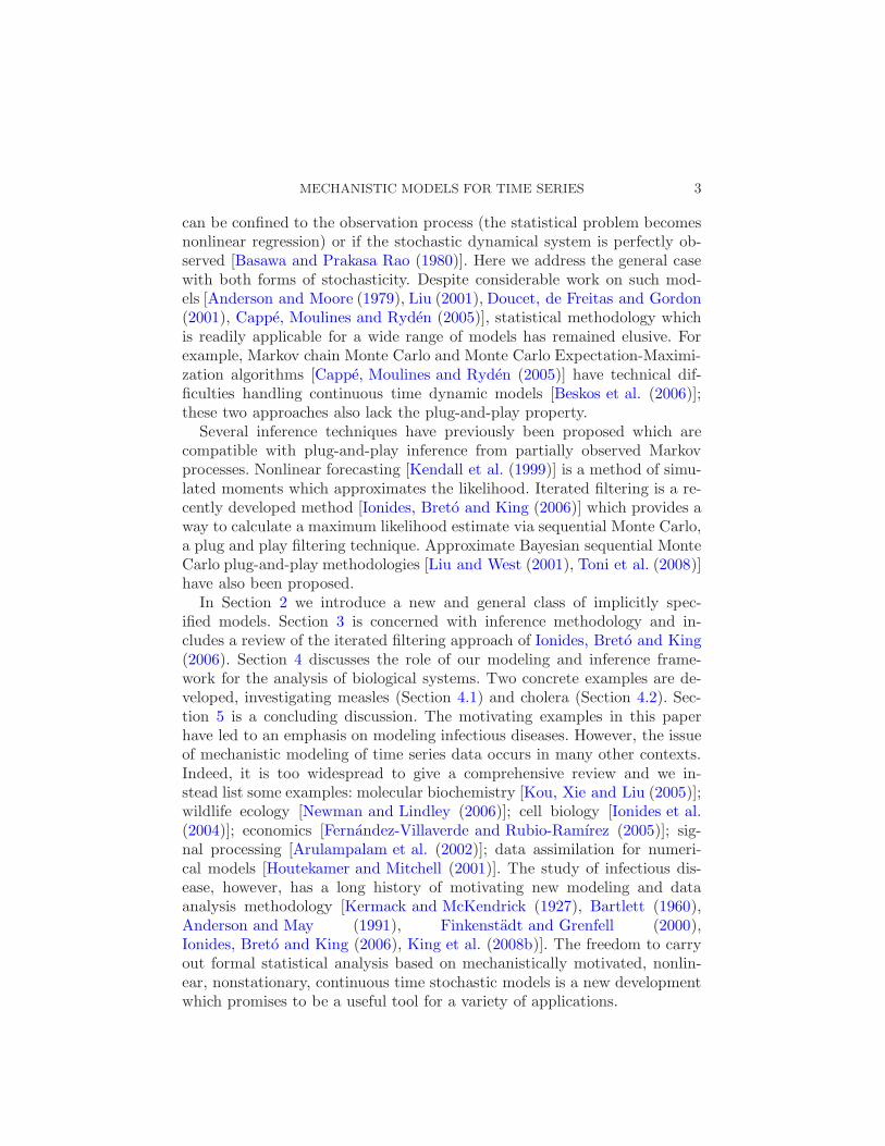
1. Divide the interval [0, T ] into N intervals of width δ = T/N2. Set initial value X(0)3. FOR n = 0 to N − 14. Generate noise increments {∆Γij = Γij(nδ + δ)− Γij(nδ)}5. Generate process increments

(∆Ni1, . . . ,∆Ni,i−1,∆Ni,i+1,∆Nic,Ri)∼Multinomial(Xi(nδ), pi1, . . . , pi,i−1,

pi,i+1, . . . , pic,1−∑

k 6=i pik)where pij = pij({µij(nδ,X(nδ))},{∆Γij}) is given in (3)

6. Set Xi(nδ + δ) = Ri +∑

j 6=i ∆Nji

7. END FOR

Fig. 1. Euler scheme for a numerical solution of the Markov chain specified by (2). Insteps 5 and 6, Ri counts the individuals who remain in compartment i during the currentEuler increment.

(P2) Stationary increments: The collection of increments {Γij(t2)−Γij(t1),1≤ i≤ c,1≤ j ≤ c} has a joint distribution depending only on t2 − t1.

(P3) Nonnegative increments: Γij(t2)− Γij(t1)≥ 0 for t2 > t1.

We have not assumed that different integrated noise processes Γij and Γkl

are independent; their increments could be correlated, or even equal. Theseintegrated noise processes define a collection of noise processes given byξij(t) = d

dtΓij(t). Since Γij(t) is increasing, ξij(t) is nonnegative and µijξij(t)

can be interpreted as a rate with multiplicative white noise. In this context,it is natural to assume the following:

(P4) Unbiased multiplicative noise: E[Γij(t)] = t.

At times, we may further assume one or more of the following properties:

(P5) Partially independent noises: For each i, {Γij(t)} is independent of{Γik(t)} for all j 6= k.

(P6) Independent noises: {Γij(t)} is independent of {Γkl(t)} for all pairs(i, j) 6= (k, l).

(P7) Gamma noises: Marginally Γij(t+δ)−Γij(t) ∼ Gamma(δ/σ2ij , σ

2ij), the

gamma distribution whose shape parameter is δ/σ2ij and scale param-

eter is σ2ij , with corresponding mean δ and variance δσ2

ij . We call σ2ij

an infinitesimal variance parameter [Karlin and Taylor (1981)].

The choice of gamma noise in (P7) gives a convenient concrete example. Awide range of Levy processes [Sato (1999)] could be alternatively employed.

We proceed to construct a compartment model as a continuous timeMarkov chain via the limit of coupled discrete-time multinomial processeswith random rates. Similar Euler multinomial schemes (without noise in


the rate function) are a standard numerical approach for studying popula-tion dynamics [Cai and Xu (2007)]. The representation of our model givenin (2) is implicit since numerical solution is available to arbitrary precisionvia evaluating the coupled multinomial processes in a discrete time-stepEuler scheme (described in Figure 1). Let ∆Nij = Nij(t + δ) − Nij(t) and∆Γij = Γij(t + δ)− Γij(t). We suppose that

P [∆Nij = nij, for all 1 ≤ i ≤ c,1 ≤ j ≤ c, i 6= j | X(t) = (x1, . . . , xc)]

= E

[

c∏

i=1

{

(

xi

ni1 · · ·nii−1nii+1 · · ·nicri

)

(

1−∑

k 6=i

pik

)ri∏

j 6=i

pnij

ij

}]

(2)

+ o(δ),

where ri = xi −∑

k 6=i nik,( nn1···nc

)

is a multinomial coefficient and

pij = pij({µij(t, x)},{∆Γij(t)})(3)

=

(

1− exp

{

−∑

k

µik∆Γik

})

µij∆Γij

/

∑

k

µik∆Γik,

with µij = µij(t, x). Theorem A.1, which is stated in Appendix A and provedin a supplement to this article [Breto et al. (2009)], shows that (2) definesa continuous time Markov chain when the conditions (P1)–(P5) hold. Afinite-state continuous time Markov chain is specified by its infinitesimaltransition probabilities [Bremaud (1999)], which are in turn specified by(2). Theorem A.2, also stated in Appendix A and proved in the supplement[Breto et al. (2009)], determines the infinitesimal transition probabilities re-sulting from (2) supposing the conditions (P1)–(P7). When the infinitesimaltransition probabilities can be calculated exactly, exact simulation methodsare available [Gillespie (1977)]. In practice, numerical schemes based on Eu-ler approximations may be preferable—Euler schemes for Markov chain com-partment models have been proposed based on Poisson [Gillespie (2001)],binomial [Tian and Burrage (2004)] and multinomial [Cai and Xu (2007)]approximations. Our choice of a model for which convenient numerical so-lutions are available (e.g., via the procedure in Figure 1) comes at the ex-pense of difficulty in computing analytic properties of the implicitly-definedcontinuous-time process. However, since the properties of the model will beinvestigated by simulation, via a plug-and-play methodology, the analyticproperties of the continuous-time process are of relatively little interest.

For the gamma noise in (P7), the special case where σij = 0 is taken tocorrespond to ξij(t) = 1. If σij = 0 for all i and j, then (2) becomes the Pois-son system widely used to model demographic stochasticity in populationmodels [Bremaud (1999), Bartlett (1960)]. We therefore call a process de-fined by (2) a Poisson system with stochastic rates. Constructions similar to


Theorem A.1 are standard for Poisson systems [Bremaud (1999)], but herecare is required to deal with the novel inclusion of white noise in the rateprocess. Our formulation for adding noise to Poisson systems can be seenas a generalization of subordinated Levy processes [Sato (1999)], though weare not aware of previous work on the more general Markov processes con-structed here. It is only the recent development of plug-and-play inferencemethodology that has led to the need for flexible Markov chain models withrandom rates.

2.1. Comments on the role of numerical solutions based on discretizations.In this section we have proposed employing a discrete-time approximationto a continuous-time stochastic process. Numerical solutions based on dis-cretizations of space and time are ubiquitous in the applied mathematicalsciences and engineering. A standard technique is to investigate whetherfurther reduction in the size of the discretization substantially affects theconclusions of the analysis. When sufficiently fine discretization is not com-putationally feasible, the numerical solutions may still have some value. Cli-mate modeling and numerical weather prediction are examples of this: suchsystems have important dynamic behavior at scales finer than any feasiblediscretization, but numerical models nevertheless have a scientific role toplay [Solomon et al. (2007)].

When numerical modeling is used as a scientific tool, conclusions aboutthe limiting continuous time model will be claimed based on properties ofthe model that are determined by simulation of realizations from the dis-cretized model. Such conclusions depend on the assumption that propertiesof the numerical solution which are stable as the numerical approximationtimestep, δ, approaches 0 should indeed be properties of the limiting con-tinuous time process. This need not always be true, which is one reason whyanalytic properties, such as Theorems A.1 and A.2, are valuable.

From another point of view, an argument for being content with a nu-merical approximation to (2) for sufficiently small δ is that there may beno scientific reason to prefer a true continuous time model over a fine dis-cretization. For example, when modeling year-to-year population dynamics,continuous time models of adequate simplicity for data analysis typicallywill not include diurnal effects. Thus, there is no particular reason to thinkthe continuous time model more credible than a discrete time model with astep of one day. One can think of a set of equations defining a continuoustime process, combined with a specified discretization, as a way of writingdown a discrete time model, rather than treating the continuous time modelas a gold standard against which all discretizations must be judged.

3. Plug-and-play inference methodology. We suppose now that the dy-namical system depends on some unknown parameter vector θ ∈ R

dθ , so that


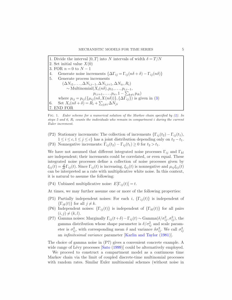
µij = µij(t, x, θ) and σij = σij(t, x, θ). Inference on θ is to be made based onobservations y1:N = (y1, . . . , yN ) made at times t1:N = (t1, . . . , tN ), with yn ∈R

dy . Conditionally on X(t1), . . . ,X(tN ), we suppose that the observationsare drawn independently from a density g(yn|X(tn), θ). Likelihood-based in-ference can be carried out for the framework of Section 2 using the iteratedfiltering methodology proposed by Ionides, Breto and King (2006), imple-mented as described in Figure 2. Iterated filtering is a technique to maximizethe likelihood for a partially observed Markov model, permitting calcula-tion of maximum likelihood point estimates, confidence intervals (via profilelikelihood, bootstrap or Fisher information) and likelihood ratio hypothesistests. Iterated filtering has been developed in response to challenges aris-ing in ecological and epidemiological data analysis [Ionides, Breto and King(2006, 2008), King et al. (2008b)], and appears here for the first time inthe statistical literature. We refer to Ionides, Breto and King (2006) for themathematical results concerning the iterated filtering algorithm in Figure 2.We proceed to review the methodology and its heuristic motivation, to dis-cuss implementation issues, and to place iterated filtering in the context ofalternative statistical methodologies.

For nonlinear non-Gaussian partially observed Markov models, the likeli-hood function can typically be evaluated only inexactly and at considerablecomputational expense. The iterated filtering procedure takes advantageof the partially observed Markov structure to enable computationally effi-cient maximization. A useful property of partially observed Markov mod-els is that, if the parameter θ is replaced by a random walk θ1:N , withE[θ0] = θ and E[θn|θn−1] = θn−1 for n > 1, the calculation of θn = E[θn|y1:n]and Vn = Var(θn|y1:n−1) is a well-studied and computationally convenient fil-tering problem [Kitagawa (1998), Liu and West (2001)]. Additional stochas-ticity of this kind is introduced in steps 4 and 12 of Figure 2. This leadsto time-varying parameter estimates, so θi(tn) in Figure 2 is an estimateof θi depending primarily on the data at and shortly before time tn. Theupdating rule in step 16, giving an appropriate way to combine these tem-porally local estimates, is the main innovative component of the procedure.Ionides, Breto and King (2006) showed that this algorithm converges to themaximum of the likelihood function, under sufficient regularity conditionsto justify a Taylor series expansion argument. Only the mean and varianceof the stochasticity added in steps 4 and 12 play a role in the limit as nincreases. The specific choice of the normal distribution for steps 4 and 12of Figure 2 is therefore unimportant, but does require that the parameterspace is unbounded. This is achieved by reparameterizing where necessary;we use a log transform for positive parameters and a logit transform forparameters lying in the interval [0,1].

Steps 2, 11 and 17 of Figure 2 concern the initial values of the state vari-ables. For stationary processes, one can think of these as unobserved random


MODEL INPUT: f(·), g(·|·), y1, . . . , yN , t0, . . . , tN

ALGORITHMIC PARAMETERS: integers J , L, M ;

scalars 0 < a < 1, b > 0; vectors X(1)I , θ(1);

positive definite symmetric matrices ΣI , Σθ.

1. FOR m = 1 to M2. XI(t0, j) ∼ N [X

(m)I , am−1ΣI ], j = 1, . . . , J

3. XF (t0, j) = XI(t0, j)4. θ(t0, j) ∼N [θ(m), bam−1Σθ]5. θ(t0) = θ(m)

6. FOR n = 1 to N7. XP (tn, j) = f(XF (tn−1, j), tn−1, tn, θ(tn−1, j),W )8. w(n, j) = g(yn|XP (tn, j), tn, θ(tn−1, j))9. draw k1, . . . , kJ such that

Prob(kj = i) = w(n, i)/∑

ℓ w(n, ℓ)10. XF (tn, j) = XP (tn, kj)11. XI(tn, j) = XI(tn−1, kj)12. θ(tn, j) ∼ N [θ(tn−1, kj), a

m−1(tn − tn−1)Σθ]13. Set θi(tn) to be the sample mean of {θi(tn−1, kj), j = 1, . . . , J}14. Set Vi(tn) to be the sample variance of {θi(tn, j), j = 1, . . . , J}15. END FOR16. θ

(m+1)i = θ

(m)i + Vi(t1)

∑Nn=1 V −1

i (tn)(θi(tn)− θi(tn−1))

17. Set X(m+1)I to be the sample mean of {XI(tL, j), j = 1, . . . , J}

18. END FOR

RETURNmaximum likelihood estimate for parameters, θ = θ(M+1)

maximum likelihood estimate for initial values, X(t0) = X(M+1)I

maximized conditional log likelihood estimates, ℓn(θ) = log(∑

j w(n, j)/J)

maximized log likelihood estimate, ℓ(θ) =∑

n ℓn(θ)

Fig. 2. Implementation of likelihood maximization by iterated filtering. N [µ,Σ] corre-sponds to a normal random variable with mean vector µ and covariance matrix Σ; X(tn)takes values in R

dx ; yn takes values in Rdy ; θ takes values in R

dθ and has components{θi, i = 1, . . . , dθ}; f(·) is the transition rule described in (4); g(·|·) is the measurementdensity for the observations y1:N .

variables drawn from the stationary distribution. However, for nonstation-ary processes (such as those considered in Sections 4.1 and 4.2, and anyprocess modeled conditional on measured covariates) these initial values aretreated as unknown parameters. These parameters require special attention,despite not usually being quantities of primary scientific interest, since the


information about them is concentrated at the beginning of the time series,whereas the computational benefit of iterated filtering arises from combin-ing information accrued through time. Steps 2, 11 and 17 implement a fixedlag smoother [Anderson and Moore (1979)] to iteratively update the initialvalue estimates. The value of the fixed lag (denoted by L in Figure 2) shouldbe chosen so that there is negligible additional information about the initialvalues after time tL. Choosing L too large results in slower convergence,choosing L too small results in bias.

Iterated filtering, characterized by the updating rule in step 16 of Fig-ure 2, can be implemented via any filtering method. The procedure inFigure 2 employs a basic sequential Monte Carlo filter which we foundto be adequate for the examples in Section 4 and also for previous dataanalyses [Ionides, Breto and King (2006), King et al. (2008b)]. Manyextensions and generalizations of sequential Monte Carlo have been pro-posed [Arulampalam et al. (2002), Doucet, de Freitas and Gordon (2001),Del Moral, Doucet and Jasra (2006)] and could be employed in an iteratedfiltering algorithm. If the filtering technique is plug-and-play, then likeli-hood maximization by iterated filtering also has this property. Basic sequen-tial Monte Carlo filtering techniques do have the plug-and-play property,since only simulations from the transition density of the dynamical systemare required and not evaluation of the density itself. Although sequentialMonte Carlo algorithms are usually written in terms of transition densities[Arulampalam et al. (2002), Doucet, de Freitas and Gordon (2001)], we em-phasize the plug-and-play property of the procedure in Figure 2 by specifyinga Markov process at a sequence of times t0 < t1 < · · · < tN via a recursivetransition rule,

X(tn) = f(X(tn−1), tn−1, tn, θ,W ).(4)

Here, it is understood that W is some random variable which is drawnindependently each time f(·) is evaluated. In the context of the plug-and-play philosophy, f(·) is the algorithm to generate a simulated sample pathof X(t) at the discrete times t1, . . . , tN given an initial value X(t0).

To check whether global maximization has been achieved, one can and

should consider various different starting values [i.e., θ(1) and X(1)I in Fig-

ure 2]. Attainment of a local maximum can be checked by investigation of the

likelihood surface local to an estimate θ. Such an investigation can also giverise to standard errors, and we describe here how this was carried out for theresults in Table 2. We write ℓ(θ) for the log likelihood function, and we call

a graph of ℓ(θ +zδi) against θi +z a sliced likelihood plot; here, δi is a vectorof zeros with a one in the ith position, and θ has components {θ1, . . . , θdθ

}.

If θ is located at a local maximum of each sliced likelihood, then θ is a localmaximum of ℓ(θ), supposing ℓ(θ) is continuously differentiable. We check


this by evaluating ℓ(θ + zijδi) for a collection {zij} defining a neighborhood

of θ. The likelihood is evaluated with Monte Carlo error, as described inFigure 2, with ΣI = 0, Σθ = 0 and M = 1. Therefore, it is necessary to makea smooth approximation to the sliced likelihood [Ionides (2005)] based onthe available evaluations. The size of the neighborhood (specified by {zij})and the size of the Monte Carlo sample (specified by J in Figure 2) shouldbe large enough that the local maximum for each slice is clearly identified.Computing sliced likelihoods requires moderate computational effort, linearin the dimension of θ. As a by-product of the sliced likelihood computation,one has access to the conditional log likelihood values, defined in Figure 2and written here as ℓnij = ℓn(θ + zijδi). Regressing ℓnij on zij for each fixed

i and n gives rise to estimates ℓni for the partial derivatives of the con-ditional log likelihoods. Standard errors of parameters are found from theestimated observed Fisher information matrix [Barndorff-Nielsen and Cox

(1994)], with entries given by Iik =∑

n ℓniℓnk. We prefer profile likelihoodcalculations, such as Figure 7, to derive confidence intervals for quantitiesof particular interest. However, standard errors derived from estimating theobserved Fisher information involve substantially less computation.

Parameter estimation for partially observed nonlinear Markov processeshas long been a challenging problem, and it is premature to expect a fullyautomated statistical procedure. The implementation of iterated filteringin Figure 2 employs algorithmic parameters which require some trial anderror to select. However, once the likelihood has been demonstrated to besuccessfully maximized, the algorithmic parameters play no role in the sci-entific interpretation of the results.

Other plug-and-play inference methodologies applicable to the models ofSection 2 have been developed. Nonlinear forecasting [Kendall et al. (1999)]has neither the statistical efficiency of a likelihood-based method nor thecomputational efficiency of a filtering-based method. The Bayesian sequen-tial Monte Carlo approximation of Liu and West (2001) combines likelihood-based inference with a filtering algorithm, but is not supported by theoret-ical guarantees comparable to those presented by Ionides, Breto and King(2006) for iterated filtering. A recently developed plug-and-play approachto approximate Bayesian inference [Sisson, Fan and Tanaka (2007)] has beenapplied to partially observed Markov processes [Toni et al. (2008)]. Other re-cent developments in Bayesian methodology for partially observed Markovprocesses include Newman et al. (2008), Cauchemez and Ferguson (2008),Cauchemez et al. (2008), Beskos et al. (2006), Polson, Stroud and Muller(2008), Boys, Wilkinson and Kirkwood (2008). This research has been mo-tivated by the inapplicability of general Bayesian software, such as WinBUGS[Lunn et al. (2000)], for many practical inference situations [Newman et al.(2008)].


A numerical implementation of iterated filtering is available via the soft-ware package pomp [King, Ionides and Breto (2008a)] which operates in thefree, open-source, R computing environment [R Development Core Team(2006)]. This package contains a tutorial vignette as well as further ex-amples of mechanistic time series models. The data analyses of Section 4were carried out using pomp, in which the algorithms in Figures 1 and 2 areimplemented via the functions reulermultinom and mif respectively.

4. Time series analysis for biological systems. Mathematical models forthe temporal dynamics of biological populations have long played a rolein understanding fluctuations in population abundance and interactionsbetween species [Bjornstad and Grenfell (2001), May (2004)]. When usingmodels to examine the strength of evidence concerning rival hypothesesabout a system, a model is typically required to capture not just the qualita-tive features of the dynamics but also to explain quantitatively all the avail-able observations on the system. A critical aspect of capturing the statisticalbehavior of data is an adequate representation of stochastic variation, whichis a ubiquitous component of biological systems. Stochasticity can also playan important role in the qualitative dynamic behavior of biological systems[Coulson, Rohani and Pascual (2004), Alonso, McKane and Pascual (2007)].Unpredictable event times of births, deaths and interactions between in-dividuals result in random variability known as demographic stochasticity(from a microbiological perspective, the individuals in question might becells or large organic molecules). The environmental conditions in whichthe system operates will fluctuate considerably in all but the best experi-mentally controlled situations, resulting in environmental stochasticity. Theframework of Section 2 provides a general way to build the phenomenon ofenvironmental stochasticity into continuous-time population models, via theinclusion of variability in the rates at which population processes occur. Toour knowledge, this is the first general framework for continuous time, dis-crete population dynamics which allows for both demographic stochasticity[infinitesimal variance equal to the infinitesimal mean; see Karlin and Taylor(1981) and Appendix B] and environmental stochasticity [infinitesimal vari-ance greater than the infinitesimal mean; see supporting online materialBreto et al. (2009)].

From the point of view of statistical analysis, environmental stochasticityplays a comparable role for dynamic population models to the role playedby over-dispersion in generalized linear models. Models which do not per-mit consideration of environmental stochasticity lead to strong assumptionsabout the levels of stochasticity in the system. This relationship is discussedfurther in Section 5. For generalized linear models, over-dispersion is com-monplace, and failure to account properly for it can give rise to misleadingconclusions [McCullagh and Nelder (1989)]. Phrased another way, including


sufficient stochasticity in a model to match the unpredictability of the datais essential if the model is to be used for forecasting, or predicting a quan-titative range of likely effects of an intervention, or estimating unobservedcomponents of the system.

We present two examples. First, Section 4.1 demonstrates the role of en-vironmental stochasticity in measles transmission dynamics, an extensivelystudied and relatively simple biological system. Second, Section 4.2 analyzesdata on competing strains of cholera to demonstrate the modeling frame-work of Section 2 and the inference methodology of Section 3 on a morecomplex system.

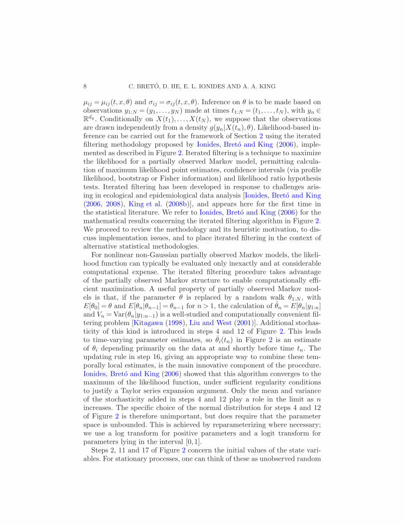
4.1. Environmental stochasticity in measles epidemics. The challengesof moving from mathematical models, which provide some insight into thesystem dynamics, to statistical models, which both capture the mechanisticbasis of the system and statistically describe the data, are welldocumented by a sequence of work on the dynamics of measles epidemics[Bartlett (1960), Anderson and May (1991), Finkenstadt and Grenfell (2000),Bjornstad, Finkenstadt and Grenfell (2002), Morton and Finkenstadt (2005),Cauchemez and Ferguson (2008)]. Measles is no longer a major developedworld health issue but still causes substantial morbidity and mortality, par-ticularly in sub-Saharan Africa [Grais et al. (2006), Conlan and Grenfell(2007)]. The availability of excellent data before the introduction ofwidespread vaccination has made measles a model epidemic system. Re-cent attempts to analyze population-level time series data on measles epi-demics via mechanistic dynamic models have, through statistical expedi-ency, been compelled to use a discrete-time dynamic model using timestepssynchronous with the reporting intervals [Finkenstadt and Grenfell (2000),Bjornstad, Finkenstadt and Grenfell (2002), Morton and Finkenstadt (2005)].Such discrete time models risk incorporating undesired artifacts [Glass,Xia and Grenfell (2003)]. The first likelihood-based analysis via continu-ous time mechanistic models, incorporating only demographic stochasticity,was published while this paper was under review [Cauchemez and Ferguson(2008)]. From another perspective, the properties of stochastic dynamic epi-demic models have been studied extensively in the context of continuoustime models with only demographic stochasticity [Bauch and Earn (2003),Dushoff et al. (2004), Wearing, Rohani and Keeling (2005)]. We go beyondprevious approaches, by demonstrating the possibility of carrying out mod-eling and data analysis via continuous time mechanistic models with bothdemographic and environmental stochasticity. For comparison with the workof Cauchemez and Ferguson (2008), we analyze measles epidemics occurringin London, England during the pre-vaccination era. The data, reported casesfrom 1948 to 1964, are shown in Figure 3.


Fig. 3. Biweekly recorded measles cases (solid line) and birth rate (dotted line, estimatedby smooth interpolation of annual birth statistics) for London, England.

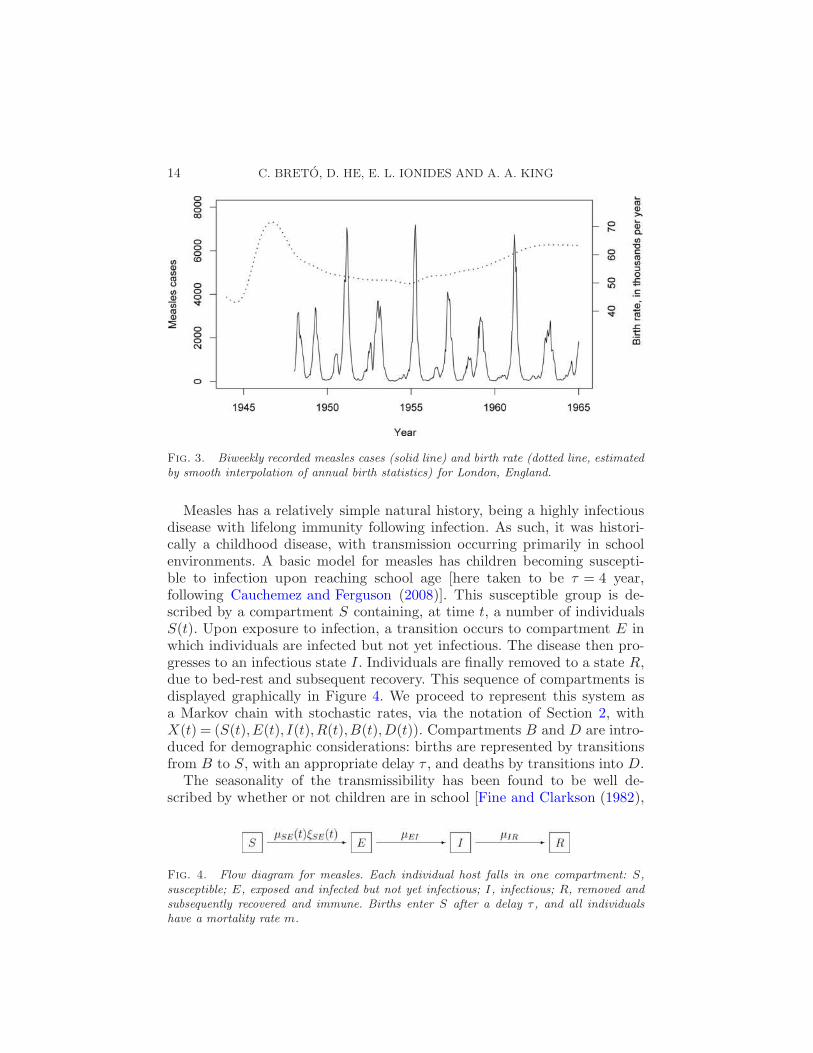
Measles has a relatively simple natural history, being a highly infectiousdisease with lifelong immunity following infection. As such, it was histori-cally a childhood disease, with transmission occurring primarily in schoolenvironments. A basic model for measles has children becoming suscepti-ble to infection upon reaching school age [here taken to be τ = 4 year,following Cauchemez and Ferguson (2008)]. This susceptible group is de-scribed by a compartment S containing, at time t, a number of individualsS(t). Upon exposure to infection, a transition occurs to compartment E inwhich individuals are infected but not yet infectious. The disease then pro-gresses to an infectious state I . Individuals are finally removed to a state R,due to bed-rest and subsequent recovery. This sequence of compartments isdisplayed graphically in Figure 4. We proceed to represent this system asa Markov chain with stochastic rates, via the notation of Section 2, withX(t) = (S(t),E(t), I(t),R(t),B(t),D(t)). Compartments B and D are intro-duced for demographic considerations: births are represented by transitionsfrom B to S, with an appropriate delay τ , and deaths by transitions into D.

The seasonality of the transmissibility has been found to be well de-scribed by whether or not children are in school [Fine and Clarkson (1982),

Fig. 4. Flow diagram for measles. Each individual host falls in one compartment: S,susceptible; E, exposed and infected but not yet infectious; I , infectious; R, removed andsubsequently recovered and immune. Births enter S after a delay τ , and all individualshave a mortality rate m.


Bauch and Earn (2003)]. Thus, we define a transmissibility function β(t) by

β(t) =

{

βH : (t) = 7–99, 116–199, 252–299, 308–355,

βL :d(t) = 356–6, 100–115, 200–251, 300–307,(5)

where d(t) is the integer-valued day (1–365) corresponding to the real-valuedtime t measured in years. This functional form allows reduced transmissionduring the Christmas vacation (days 356–365 and 1–6), Easter vacation(100–115), Summer vacation (200–251) and Autumn half-term (300–307).The rate of new infections is given the form

µSE = β(t)[I(t) + ω]α/P (t).(6)

Here, ω describes infection from measles cases outside the population understudy; α describes inhomogeneous mixing [Finkenstadt and Grenfell (2000)];P (t) is the total population size, which is treated as a known covariate viainterpolation from census data. Environmental stochasticity on transmissionis included via a gamma noise process ξSE(t) with infinitesimal variance pa-rameter σ2

SE ; transmission is presumed to be the most variable process inthe system, and other transitions are taken to be noise-free. The two otherdisease parameters, µEI and µIR, are treated as unknown constants. We sup-pose a constant mortality rate, µSD = µED = µID = µRD = m, and here wefix m = 1/50 year−1. The recruitment of school-age children is specified bythe process NBS(t) = ⌊

∫ t0 b(s− τ)ds⌋, where b(t) is the birth rate, presented

in Figure 3, and ⌊x⌋ is the integer part of x. We note that the constructionabove does not perfectly match the constraint S(t) + E(t) + I(t) + R(t) =P (t). For a childhood disease, such as measles, a good estimate of the birthrate is important, whereas the system is insensitive to the exact size of theadult population.

All transitions not mentioned above are taken to have a rate of zero.To complete the model specification, a measurement model is required. Bi-weekly aggregated measles cases are denoted by Cn = NIR(tn)−NIR(tn−1)with tn being the time, in years, of the nth observation. Reporting ratesρn are taken to be independent Gamma(1/φ, ρφ) random variables. Condi-tional on ρn, the observations are modeled as independent Poisson counts,Yn|ρn,Cn ∼ Poisson(ρnCn). Thus, Yn given Cn has a negative binomial dis-tribution with E[Yn|Cn] = ρCn and Var(Yn|Cn) = ρCn + φρ2C2

n. Note thatthe measurement model counts transitions into R, since individuals are re-moved from the infective pool (treated with bed-rest) once diagnosed. Themeasurement model allows for the possibility of both demographic stochas-ticity (i.e., Poisson variability) and environmental stochasticity (i.e., gammavariability on the rates).

A likelihood ratio test concludes that, in the context of this model, en-vironmental stochasticity is clearly required to explain the data: the log


likelihood for the full model was found to be −2504.9, compared to −2662.0for the restricted model with σSE = 0 (p < 10−6, chi-square test; resultsbased on a time-step of δ = 1 day in the Euler scheme of Figure 1 and aMonte Carlo sample size of J = 20000 when carrying out the iterated filter-ing algorithm in Figure 2). Future model-based scientific investigations ofdisease dynamics should consider environmental stochasticity when basingscientific conclusions on the results of formal statistical tests.

Environmental stochasticity, like over-dispersion in generalized linear mod-els, is more readily detected than scientifically explained. Teasing apartthe extent to which environmental stochasticity is describing model mis-specification rather than random phenomena in the system is beyond thescope of the present paper. The inference framework developed here willfacilitate both asking and answering such questions. However, this distinc-tion is not relevant to the central statistical question of whether a particularclass of scientifically motivated models requires environmental stochasticity(in the broadest sense of a source of variability above and beyond demo-graphic stochasticity) to explain the data. Models of biological systems arenecessarily simplifications of complex processes [May (2004)], and as such, itis a legitimate role for environmental stochasticity to represent and quantifythe contributions of unknown and/or unmodeled processes to the systemunder investigation.

The environmental stochasticity identified here has consequences for thequalitative understanding of measles epidemics. Bauch and Earn (2003) havepointed out that demographic stochasticity is not sufficient to explain thedeviations which historically occurred from periodic epidemics (at one, twoor three year cycles, depending on the population size and the birth-rate).Simulations from the fitted model with environmental stochasticity are ableto reproduce such irregularities (results not shown), giving a simple expla-nation of this phenomenon. This does not rule out the possibility that someother explanation, such as explicitly introducing a new covariate into themodel, could give an even better explanation.

In agreement with Cauchemez and Ferguson (2008), we have found thatsome combinations of parameters in our model are only weakly identifiable(i.e., they are formally identifiable, but have broad confidence intervals).Although this does not invalidate the above likelihood ratio test, it doescause difficulties interpreting parameter estimates. In the face of this prob-lem, Cauchemez and Ferguson (2008) made additional modeling assump-tions to improve identifiability of unknown parameters. Here, our goal is todemonstrate our modeling and inference framework, rather than to presenta comprehensive investigation of measles dynamics.

The analysis of Cauchemez and Ferguson (2008), together with other con-tributions by the same authors [Cauchemez et al. (2008, 2006)], representsthe state of the art for Markov chain Monte Carlo analysis of population


dynamics. Whereas Cauchemez and Ferguson (2008) required model-specificapproximations and analytic calculations to carry out likelihood-based infer-ence via their Markov chain Monte Carlo approach, our analysis is a routineapplication of the general framework in Sections 2 and 3. Our methodol-ogy also goes beyond that of Cauchemez and Ferguson (2008) by allowingthe consideration of environmental stochasticity, and the inclusion of thedisease latent period (represented by the compartment E) which has beenfound relevant to the disease dynamics [Finkenstadt and Grenfell (2000),Bjornstad, Finkenstadt and Grenfell (2002), Morton and Finkenstadt (2005)].Furthermore, our approach generalizes readily to more complex biologicalsystems, as demonstrated by the following example.

4.2. A mechanistic model for competing strains of cholera. All infec-tious pathogens have a variety of strains, and a good understanding ofthe strain structure can be key to understanding the epidemiology of thedisease, understanding evolution of resistance to medication, and devel-oping effective vaccines and vaccination strategies [Grenfell et al. (2004)].Previous analyses relating mathematical consequences of strain structureto disease data include studies of malaria [Gupta et al. (1994)], dengue[Ferguson, Anderson and Gupta (1999)], influenza [Ferguson, Galvani and Bush(2003), Koelle et al. (2006a)] and cholera [Koelle, Pascual and Yunus (2006b)].For measles, the strain structure is considered to have negligible importancefor the transmission dynamics [Conlan and Grenfell (2007)], another reasonwhy measles epidemics form a relatively simple biological system. In thissection, we demonstrate that our mechanistic modeling framework permitslikelihood based inference for mechanistically motivated stochastic modelsof strain-structured disease systems, and that the results can lead to freshscientific insights.

There are many possible immunological consequences of the presence ofmultiple strains, but it is often the case that exposure of a host to onestrain of a pathogen results in some degree of protection (immunity) from re-infection by that strain and, frequently, somewhat weaker protection (cross-immunity) from infection by other strains. Immunologically distinct strainsare called serotypes. In the case of cholera, there are currently two commonserotypes, Inaba and Ogawa. Koelle, Pascual and Yunus (2006b), followingthe multistrain modeling approach of Kamo and Sasaki (2002), constructeda mechanistic, deterministic model of cholera transmission and immunity toinvestigate the pattern of changes in serotype dominance observed in choleracase report data collected in an intensive surveillance program conducted bythe International Center for Diarrheal Disease Research, Bangladesh. Theyargued on the basis of a comparison of the data with features of typical tra-jectories of the dynamical model. Specifically, Koelle, Pascual and Yunus(2006b) found that the model would exhibit behavior which approximately


Fig. 5. Biweekly cholera cases obtained from hospital records of the International Centerfor Diarrheal Disease Research, Bangladesh for the district of Matlab, Bangladesh, 55 kmSE of Dhaka. Cases are categorized into serotypes, Inaba (dashed) and Ogawa (solid gray).Each serotype may be further classified into one of two biotypes, El Tor and Classical, whichare combined here, following Koelle et al. (2006b). The total population size of the district,in thousands, is shown as a dotted line.

matched the period of cycles in strain dominance only when the cross-immunity was high, that is, when the probability of cross-protection wasapproximately 0.95. In addition, they found that their model’s behavior de-pended very sensitively on the cross-immunity parameter. Here we employformal likelihood-based inference on the same data to assess the strength ofthe evidence in favor of these conclusions.

Fig. 6. Flow diagram for cholera, including interactions between the two major serotypes.Each individual host falls in one compartment: S, susceptible to both Inaba and Ogawaserotypes; I1, infected with Inaba; I2, infected with Ogawa; S1, susceptible to Inaba (butimmune to Ogawa); S2, susceptible to Ogawa (but immune to Inaba); I∗

1 , infected withInaba (but immune to Ogawa); I∗

2 , infected with Ogawa (but immune to Inaba); R, immuneto both serotypes. Births enter S, and all individuals have a mortality rate m.


We analyzed a time series consisting of 30 years of biweekly cholera inci-dence records (Figure 5). For each cholera case, the serotype of the infect-ing strain—Inaba or Ogawa—was determined. We formulated a stochasticversion of the model analyzed by Koelle, Pascual and Yunus (2006b). Themodel is shown diagrammatically in Figure 6, in which arrows represent pos-sible transitions, each labeled with the corresponding rate of flow. Table 1specifies the model formally, in the framework of Section 2, as a Markov chainwith stochastic rates. The parameters in the model have standard epidemio-logical interpretations [Anderson and May (1991), Finkenstadt and Grenfell(2000), Koelle and Pascual (2004)]: λ1 is the force of infection for the In-aba serotype, that is, the mean rate at which susceptible individuals becomeinfected; ξ1 is the stochastic noise on this rate; λ2 and ξ2 are the correspond-ing force of infection and noise for the Ogawa serotype; β(t) is the rate oftransmission between individuals, parameterized with a linear trend and asmooth seasonal component; ω gives the rate of infection from an environ-mental reservoir, independent of the current number of contagious individu-als; the exponent α allows for inhomogeneous mixing of the population; r isthe recovery rate from infection; γ measures the strength of cross-immunitybetween serotypes. In this model, as in Koelle, Pascual and Yunus (2006b),infection with a given serotype results in life-long immunity to reinfectionby that serotype. The argument for giving both strains common variabil-ity is that they are believed to be biologically similar except in regard toimmune response. The strains have independent noise components becausethe noise represents chance events, such as a contaminated feast or a singlecommunity water source which is transiently in a favorable condition forcontamination, and such events spread whichever strain is in the requiredplace at the required time.

To complete the model specification, we adopt an extension of the neg-ative binomial measurement model used for measles in Section 4.1. Bi-weekly aggregated cases for Inaba and Ogawa strains are denoted by Ci,n =NSIi(tn)−NSIi(tn−1) + NSiI

∗i(tn)−NSiI

∗i(tn−1) for i = 1,2 respectively and

tn = 1975 + n/24. Reporting rates ρ1,n and ρ2,n are taken to be indepen-dent Gamma(1/φ, ρφ) random variables. Conditional on ρ1,n and ρ2,n, theobservations are modeled as independent Poisson counts,

Yi,n|ρi,n,Ci,n ∼Poisson(ρi,nCi,n), i = 1,2.

Thus, Yi,n given Ci,n has a negative binomial distribution with E[Yi,n|Ci,n] =ρCi,n and Var(Yi,n|Ci,n) = ρCi,n + φρ2C2

i,n.Some results from fitting the model in Figure 6 via the method in Fig-

ure 2 are shown in Table 2. The two sets of parameter values θA and θB inTable 2 are maximum likelihood estimates, with θA having the additionalconstraints ρ = 0.067 and r = 38.4. These two constraints were imposed by


Table 1

Interpretation of Figure 6 via the multinomial process with random rates in (2), withX(t) = (S(t), I1(t), I2(t), S1(t), S2(t), I∗

1 (t), I∗2 (t), R(t), B(t), D(t)). Compartments B

and D are introduced for demographic considerations: births are formally treated astransitions from B to S and deaths as transitions into D. All transitions not listed above

have zero rate. ξ2(t) and ξ1(t) are independent gamma noise processes, each withinfinitesimal variance parameter σ2. Transition rates are noise-free unless specified

otherwise. Seasonality is modeled via a periodic cubic B-spline basis {si(t), i = 1, . . . ,6},where si(t) attains its maximum at t = (i− 1)/6. The population size P (t) is shown inFigure 5. The birth process is treated as a covariate, that is, the analysis is carried out

conditional on the process NBS(t) = ⌊P (t)− P (0) +∫ t

0mP (s)ds⌋, where ⌊x⌋ is the

integer part of x. There is a small stochastic discrepancy betweenS(t) + I1(t) + I2(t) + S1(t) + S2(t) + I∗

1 (t) + I∗2 (t) + R(t) and P (t). In principle, one

could condition on the demographic data by including a population measurementmodel—we saw no compelling reason to add this extra complexity for the current

purposes. Numerical solutions of sample paths were calculated using the algorithm inFigure 1, with δ = 2/365

λ1 = β(t)(I1(t) + I∗1 (t))α/P (t) + ω

λ2 = β(t)(I2(t) + I∗2 (t))α/P (t) + ω

log β(t) = b0(t− 1990) +∑6

i=1bisi(t)

µSI1 = λ1

µSI2 = λ2

µS1I∗

1= (1− γ)λ1

µS2I∗

2= (1− γ)λ2

µI1S2= µI2S1

= rµI∗

2R = µI∗

1R = r

µXjD = m for Xj ∈ {S, I1, I2, S1, S2, I∗1 , I∗

2 ,R}ξSI2 = ξS2I∗

2= ξ2(t)

ξSI1 = ξS1I∗

1= ξ1(t)

Koelle, Pascual and Yunus (2006b), based on previous literature. The fit-ted model with the additional constraints is qualitatively different from theunconstrained model, and we refer to the neighborhoods of these two pa-rameter sets as regimes A and B. Figure 7 shows a profile likelihood forcross-immunity in regime A; this likelihood-based analysis leads to substan-tially lower cross-immunity than the estimate of Koelle, Pascual and Yunus(2006b). In regime B, the cross-immunity is estimated as being complete(γ = 1), however, the corresponding standard error is large: cross-immunityis poorly identified in regime B since the much higher reporting rate (ρ =0.65) means that there are many fewer cases and so few individuals are everexposed to both serotypes.

These two regimes demonstrate two distinct uses of a statistical model—first, to investigate the consequences of a set of assumptions and, second,to challenge those assumptions. If we take for granted the published esti-mates of certain parameter values, the resulting parameter estimates θA arebroadly consistent with previous models for cholera dynamics in terms of


Table 2

Parameter estimates from both regimes. In both regimes, the mortality rate m is fixed at1/38.8 years−1. The units of r, b0 and ω are year−1; σ has units year1/2; and ρ, γ, φ, αand b1, . . . , b6 are dimensionless. ℓ is the average of two log-likelihood evaluations using a

particle filter with 120,000 particles. Optimization was carried out using the iteratedfiltering in Figure 2, with M = 30, a = 0.95 and J = 15,000. Optimization parameters

were selected via diagnostic convergence plots [Ionides, Breto and King (2006)]. Standarderrors (SEs) were derived via a Hessian approximation; this is relatively rapid to

compute and gives a reasonable idea of the scale of uncertainty, but profile likelihoodbased confidence intervals are more appropriate for formal inference

θA SEA θB SEB

r 38.42 – 36.91 3.88ρ 0.067 – 0.653 0.069γ 0.400 0.087 1.00 0.41σ 0.1057 0.0076 0.0592 0.0075φ 0.014 0.30 0.0004 0.024ω × 103 0.099 0.022 0.0762 0.0072α 0.860 0.015 0.864 0.017b0 −0.0275 0.0017 −0.0209 0.0015b1 4.608 0.098 3.507 0.083b2 5.342 0.074 3.733 0.091b3 5.723 0.075 4.448 0.055b4 5.022 0.076 3.534 0.065b5 5.508 0.064 4.339 0.053b6 5.804 0.059 4.274 0.039ℓ −3560.23 −3539.11

the fraction of the population which has acquired immunity to cholera andthe fraction of cases which are asymptomatic (a term applied to the ma-jority of unreported cases which are presumed to have negligible symptomsbut are nevertheless infectious). However, the likelihood values in Table 2call into question the assumptions behind regime A, since the data are bet-ter explained by regime B (p < 10−6, likelihood ratio test), for which theepidemiologically relevant cases are only the severe cases that are likely toresult in hospitalization. Unlike in regime A, asymptomatic cholera casesplay almost no role in regime B, since the reporting rate is an order of mag-nitude higher. The contrast between these regimes highlights a conceptuallimitation of compartment models: in point of fact, disease severity and levelof infectiousness are continuous, not discrete or binary as they must be inbasic compartment models. For example, differences in the level of morbid-ity required to be classified as “infected” result in re-interpretation of theparameters of the model, with consequent changes to fundamental modelcharacteristics such as the basic reproductive ratio of an infectious disease[Anderson and May (1991)]. Despite this limitation, it remains the case that


Fig. 7. Cross-immunity profile likelihood for regime A, yielding a 99% confidence inter-val for γ of (0.20, 0.61) based on a χ2 approximation [e.g., Barndorff-Nielsen and Cox(1994)]. Each point corresponds to an optimization carried out as described in the cap-tion of Table 2. Local quadratic regression implemented in R via loess with a span of 0.6[R Development Core Team (2006)] was used to estimate the profile likelihood, followingIonides (2005).

compartment models are a fundamental platform for current understandingof disease dynamics and so identification and comparison of different inter-pretations is an important exercise.

The existence of regime B shows that there is room for improvement in themodel by departing from the assumptions in regime A. Extending the modelto include differing levels of severity might permit a combination of the data-matching properties of B with the scientific interpretation of A. Other as-pects of cholera epidemiology [Sack et al. (2004), Kaper, Morris and Levine(1995)], not included in the models considered here, might affect the conclu-sions. For example, although we have followed Koelle, Pascual and Yunus(2006b) by assuming lifelong immunity following exposure to cholera, in re-ality this protection is believed to wane over time [King et al. (2008b)]. Itis plain, however, that any such model modification can be subsumed inthe modeling framework presented here and that effective inference for suchmodels is possible using the same techniques.

5. Discussion. This paper has focused on compartment models, a flexi-ble class of models which provides a broad perspective on the general topicof mechanistic models. The developments of this paper are also relevantto other systems. For example, compartment models are closely related tochemodynamic models, in which a Markov process is used to represent the


quantities of several chemical species undergoing transformations by chemi-cal reactions. The discrete nature of molecular counts can play a role, partic-ularly for large biological molecules [Reinker, Altman and Timmer (2006),Boys, Wilkinson and Kirkwood (2008)]. Our approach to stochastic transi-tion rates (Section 2) could readily be extended to chemodynamic models,and would allow for the possibility of over-dispersion in experimental sys-tems.

Given rates µij , one interpretation of a compartment model is to writethe flows as coupled ordinary differential equations (ODEs),

d

dtNij = µijXi(t).(7)

Data analysis via ODE models has challenges in its own right [Ramsay et al.(2007)]. One can include stochasticity in (7) by adding a slowly varyingfunction to the derivative [Swishchuk and Wu (2003)]. Alternatively, onecan add Gaussian white noise to give a set of coupled stochastic differentialequations (SDEs) [e.g., Øksendal (1998)]. For example, if {Wijk(t)} is acollection of independent standard Brownian motion processes, and σijk =σijk(t,X(t)), an SDE interpretation of a compartment model is given by

dNij = µijXi(t)dt +∑

k

σijk dWijk.

SDEs have some favorable properties for mechanistic modeling, such asthe ease with which stochastic models can be written down and inter-preted in terms of infinitesimal mean and variance [Ionides et al. (2004),Ionides, Breto and King (2006)]. However, there are several reasons to pre-fer integer-valued stochastic processes over SDEs for modeling populationprocesses. Populations consist of discrete individuals, and, when a popula-tion becomes small, that discreteness can become important. For infectiousdiseases, there may be temporary extinctions, or “fade-outs,” of the diseasein a population or sub-population. Even if the SDE is an acceptable ap-proximation to the disease dynamics, there are technical reasons to prefera discrete model. Standard methods allow exact simulation for continuoustime Markov chains [Bremaud (1999), Gillespie (1977)], whereas for a non-linear SDE this is at best difficult [Beskos et al. (2006)]. In addition, if anapproximate Euler solution for a compartment model is required, nonneg-ativity constraints can more readily be accommodated for Markov chainmodels, particularly when the model is specified by a limit of multinomialapproximations, as in (2). The most basic discrete population compartmentmodel is the Poisson system [Bremaud (1999)], defined here by

P [∆Nij = nij|X(t) = (x1, . . . , xc)](8)

=∏

i

∏

j 6=i

(µijxiδ)nij (1− µijxiδ) + o(δ).


The Poisson system is a Markov chain whose transitions consist of singleindividuals moving between compartments, that is, the infinitesimal proba-bility is negligible of either simultaneous transitions between different pairsof compartments or multiple transitions between a given pair of compart-ments. As a consequence of this, the Poisson system is “equidispersed,”meaning that the infinitesimal mean of the increments equals the infinites-imal variance (Appendix B). Overdispersion is routinely observed in data[McCullagh and Nelder (1989)], and this leads us to consider models such as(2) for which the infinitesimal variance can exceed the infinitesimal mean.For infinitesimally over-dispersed systems, instantaneous transitions of morethan one individual are possible. This may be scientifically plausible: acholera-infected meal or water-jug may lead to several essentially simul-taneous cases; many people could be simultaneously exposed to an influenzapatient on a crowded bus. Quite aside from this, if one wishes for what-ever reason to write down an over-dispersed Markov model, the inclusionof such possibilities is unavoidable. Simultaneity in the limiting continuoustime model can alternatively be justified by arguing that the model onlyclaims to capture macroscopic behavior over sufficiently long time intervals.

Note that the multinomial distribution used in (2) could be replaced byalternatives, such as Poisson or negative binomial. These alternatives aremore natural for unbounded processes, such as birth processes. For equidis-persed processes, that is, without adding white noise to the rates, the limitin (2) is the same if the multinomial is replaced by Poisson or negative bi-nomial. For overdispersed processes, these limits differ. In particular, thePoisson gamma and negative binomial gamma limits have unbounded jumpdistributions and so are less readily applicable to finite populations.

The approach in (2) of adding white noise to the transition rates differsfrom previous approaches of making the rates a slowly varying random func-tion of time, that is, adding low frequency “red noise” to the rates. Thereare several motivations for introducing models based on white noise. Mostsimply, adding white noise can lead to more parsimonious parameterization,since the intensity but not the spectral shape of the noise needs to be con-sidered. The Markov property of white noise is inherited by the dynamicalsystem, allowing the application of the extensive theory of Markov chains.White noise can also be used as a building block for constructing colorednoise, for example, by employing an autoregressive model for the param-eters. At least for the specific examples of measles and cholera studied inSection 4, high-frequency variability in the rate of infection helps to explainthe data (this was explicitly tested for measles; for our cholera models, Ta-ble 2 shows that the estimates of the environmental stochasticity parameterσ are many standard errors from zero). Although variability in rates will notalways be best modeled using white noise, there are many circumstances inwhich it is useful to be able to do so.


This article has taken a likelihood-based, non-Bayesian approach to sta-tistical inference. Many of the references cited follow the Bayesian paradigm.The examples of Section 4 and other recent work [Ionides, Breto and King(2006), King et al. (2008b)] show that iterated filtering methods enable rou-tine likelihood-based inference in some situations that have been challengingfor Bayesian methodology. Bayesian and non-Bayesian analyses will continueto provide complementary approaches to inference for time series analysisvia mechanistic models, as in other areas of statistics.

Time series analysis is, by tradition, data oriented, and so the quantityand quality of available data may limit the questions that the data can rea-sonably answer. This forces a limit on the number of parameters that can beestimated for a model. Thus, a time series model termed mechanistic mightbe a simplification of a more complex model which more fully describesreductionist scientific understanding of the dynamical system. As one exam-ple, one could certainly argue for including age structure or other populationinhomogeneities into Figure 6. Indeed, determining which additional modelcomponents lead to important improvement in the statistical description ofthe observed process is a key data analysis issue.

APPENDIX A: THEOREMS CONCERNING COMPARTMENTMODELS WITH STOCHASTIC RATES

Theorem A.1. Assume (P1)–(P5) and suppose that µij(t, x) is uni-formly continuous as a function of t. Suppose initial values X(0) = (X1(0),. . . ,Xc(0)) are given and denote the total number of individuals in the popu-lation by S =

∑

i Xi(0). Label the individuals 1, . . . , S and the compartments1, . . . , c. Let C(ζ,0) be the compartment containing individual ζ at timet = 0. Set τζ,0 = 0, and generate independent Exponential(1) random vari-ables Mζ,0,j for each ζ and j 6= C(ζ,0). We will define τζ,m,j , τζ,m, C(ζ,m),and Mζ,m,j recursively for m ≥ 1. Set

τζ,m,j = inf

{

t :

∫ t

τζ,m−1

µC(ζ,m−1),j(s,X(s))dΓC(ζ,m−1),j(s) > Mζ,m−1,j

}

.(9)

At time τζ,m = minj τζ,m,j , set C(ζ,m) = argminj τζ,m,j and for each j 6=C(ζ,m) generate an independent Exponential(1) random variable Mζ,m,j .Set

dNij(t) =∑

ζ,m

I{C(ζ,m− 1) = i,C(ζ,m) = j, τζ,m = t},

where I{·} is an indicator function, and set Xi(t) = Xi(0) +∫ t0

∑

j 6=i(dNji −dNij). X(t) is a Markov chain whose infinitesimal transition probabilitiessatisfy (2).


Note A.1. The random variables {Mζ,m,j} in Theorem A.1 are termedtransition clocks, with the intuition that X(t) jumps when one (or more)of the integrated transition rates in (9) exceeds the value of its clock. In amore basic construction of a Markov chain, one re-starts the clocks for eachindividual whenever X(t) makes a transition. The memoryless property ofthe exponential distribution makes this equivalent to the construction ofTheorem A.1, where clocks are restarted only for individuals who make atransition [Sellke (1983)]. Sellke’s construction is convenient for the proof ofTheorem A.1.

Note A.2. The trajectories of the individuals are coupled through thedependence of µ(t,X(t)) on X(t), and through the noise processes whichare shared for all individuals in a given compartment and may be dependentbetween compartments. Thus, to evaluate (9), it is necessary to keep trackof all individuals simultaneously. To check that the integral in (9) is welldefined, we note that X(s) depends only on {(τζ,m,C(ζ,m)) : τζ,m ≤ s, ζ =1, . . . , S,m = 1,2, . . .}. X(s) is thus a function of events occurring by time s,so it is legitimate to use X(s) when constructing events that occur at t > s.

Theorem A.2. Supposing (P1)–(P7), the infinitesimal transition prob-abilities given by (2) are

P [∆Nij = nij, for all i 6= j |X(t) = (x1, . . . , xc)]

=∏

i

∏

j 6=i

π(nij, xi, µij, σij) + o(δ),

where

π(n,x,µ,σ)(10)

= 1{n=0} + δ

(

xn

) n∑

k=0

(

nk

)

(−1)n−k+1σ−2 ln(1 + σ2µ(x− k)).

The full independence of {Γij} assumed in Theorem A.2 gives a formfor the limiting probabilities where multiple individuals can move simulta-neously between some pair of compartments i and j, but no simultaneoustransitions occur between different compartments. In more generality, thelimiting probabilities do not have this simple structure. In the setup forTheorem A.1, where Γij is independent of Γik for j 6= k, no simultaneoustransitions occur out of some compartment i into different compartmentsj 6= k, but simultaneous transitions from i to j and from i′ to j′ cannot beruled out for i 6= i′. The assumption in Theorem A.1 that Γij is independentof Γik for j 6= k is not necessary for the construction of a process via (2),


but simplifies the subsequent analysis. Without this assumption, a construc-tion similar to Theorem A.1 would have to specify a rule for what happenswhen an individual who has two simultaneous event times, that is, whenminj τζ,m,j is not uniquely attained. Although independence assumptionsare useful for analytical results, a major purpose of the formulation in (2) isto allow the practical use of models that surpass currently available math-ematical analysis. In particular, it may be natural for different transitionprocesses to share the same noise process, if they correspond to transitionsbetween similar pairs of states.

APPENDIX B: EQUIDISPERSION OF POISSON SYSTEMS

For the Poisson system in (8),

P [∆Nij = 0|X(t) = x] = 1− µijxiδ + o(δ),(11)

P [∆Nij = 1|X(t) = x] = µijxiδ + o(δ),(12)

where x = (x1, . . . , xc) and µij = µij(t, x). Since the state space of X(t) is fi-nite, it is not a major restriction to suppose that there is some uniform boundµij(t, x)xi ≤ ν, and that the terms o(δ) in (11), (12) are uniform in x andt. Then, P [∆Nij > k|X(t)] ≤ F (k, δν), where F (k,λ) =

∑∞j=k+1 λje−λ/j!. It

follows that

E[∆Nij |X(t) = x] =∞∑

k=0

P [∆Nij > k|X(t) = x] = µijxiδ + o(δ),

E[(∆Nij)2|X(t) = x] =

∞∑

k=0

(2k + 1)P [∆Nij > k|X(t) = x] = µijxiδ + o(δ),

and so Var(∆Nij |X(t) = x) = µijxiδ + o(δ). If the rate functions µij(t, x) arethemselves stochastic, with X(t) being a conditional Markov chain given{µij ,1 ≤ i ≤ c,1 ≤ j ≤ c}, a similar calculation applies so long as a uniformbound ν still exists. In this case,

E[∆Nij |X(t) = x] = δE[µij(t, x)xi] + o(δ),(13)

Var(∆Nij |X(t) = x) = δE[µij(t, x)xi] + o(δ).(14)

The necessity of the uniform bound ν is demonstrated by the inconsistencybetween (13), (14) and the result in Theorem A.2 for the addition of whitenoise to the rates.

Acknowledgments. This work was stimulated by the working groups on“Inference for Mechanistic Model” and “Seasonality of Infectious Diseases”at the National Center for Ecological Analysis and Synthesis, a Centerfunded by NSF (Grant DEB-0553768), the University of California, Santa


Barbara, and the State of California. We thank Mercedes Pascual for dis-cussions on multi-strain modeling. We thank the editor, associate editor andreferee for their helpful suggestions. The cholera data were kindly providedby the International Centre for Diarrheal Disease Research, Bangladesh.

SUPPLEMENTARY MATERIAL

Theorems concerning compartment models with stochastic rates (DOI:10.1214/08-AOAS201SUPP; .pdf). We present proofs of Theorems A.1 and A.2,which were stated in Appendix A.

REFERENCES

Alonso, D., McKane, A. J. and Pascual, M. (2007). Stochastic amplification in epi-demics. J. R. Soc. Interface 4 575–582.

Anderson, B. D. and Moore, J. B. (1979). Optimal Filtering. Prentice-Hall, EnglewoodCliffs, NJ.

Anderson, R. M. and May, R. M. (1991). Infectious Diseases of Humans. Oxford Univ.Press.

Arulampalam, M. S., Maskell, S., Gordon, N. and Clapp, T. (2002). A tutorial onparticle filters for online nonlinear, non-Gaussian Bayesian tracking. IEEE Transactionson Signal Processing 50 174–188.

Barndorff-Nielsen, O. E. and Cox, D. R. (1994). Inference and Asymptotics. Chap-man and Hall, London. MR1317097

Bartlett, M. S. (1960). Stochastic Population Models in Ecology and Epidemiology.Wiley, New York. MR0118550

Basawa, I. V. and Prakasa Rao, B. L. S. (1980). Statistical Inference for StochasticProcesses. Academic Press, London. MR0586053

Bauch, C. T. and Earn, D. J. D. (2003). Transients and attractors in epidemics. Proc.R. Soc. Lond. B 270 1573–1578.

Beskos, A., Papaspiliopoulos, O., Roberts, G. and Fearnhead, P. (2006). Exactand computationally efficient likelihood-based inference for discretely observed diffusionprocesses. J. R. Stat. Soc. Ser. B Stat. Methodol. 68 333–382. MR2278331

Bjornstad, O. N., Finkenstadt, B. F. and Grenfell, B. T. (2002). Dynamics ofmeasles epidemics: Estimating scaling of transmission rates using a time series SIRmodel. Ecological Monographs 72 169–184.

Bjornstad, O. N. and Grenfell, B. T. (2001). Noisy clockwork: Time series analysisof population fluctuations in animals. Science 293 638–643.

Boys, R. J., Wilkinson, D. J. and Kirkwood, T. B. L. (2008). Bayesian inference fora discretely observed stochastic kinetic model. Statist. Comput. 18 125–135.

Bremaud, P. (1999). Markov Chains: Gibbs Fields, Monte Carlo Simulation, and Queues.Springer, New York. MR1689633

Breto, C., He, D., Ionides, E. L. and King, A. A. (2009). Supplement to “Time seriesanalysis via mechanistic models.” DOI: 10.1214/08-AOAS201SUPP.

Brillinger, D. R. (2008). The 2005 Neyman lecture: Dynamic indeterminism in science.Statist. Sci. 23 48–64.

Cai, X. and Xu, Z. (2007). K-leap method for accelerating stochastic simulation of coupledchemical reactions. J. Chem. Phys. 126 074102.

Cappe, O., Moulines, E. and Ryden, T. (2005). Inference in Hidden Markov Models.Springer, New York. MR2159833

http://dx.doi.org/10.1214/08-AOAS201SUPP

http://www.ams.org/mathscinet-getitem?mr=1317097





http://dx.doi.org/10.1214/08-AOAS201SUPP



Cauchemez, S. and Ferguson, N. M. (2008). Likelihood-based estimation of continuous-time epidemic models from time-series data: Application to measles transmission in

London. J. R. Soc. Interface 5 885–897.Cauchemez, S., Temime, L., Guillemot, D., Varon, E., Valleron, A.-J.,

Thomas, G. and Boelle, P.-Y. (2006). Investigating heterogeneity in pneumococ-

cal transmission: A Bayesian MCMC approach applied to a follow-up of schools. J.Amer. Statist. Assoc. 101 946–958. MR2324106

Cauchemez, S., Valleron, A., Boelle, P., Flahault, A. and Ferguson, N. M.

(2008). Estimating the impact of school closure on influenza transmission from sentineldata. Nature 452 750–754.

Conlan, A. and Grenfell, B. (2007). Seasonality and the persistence and invasion ofmeasles. Proc. R. Soc. Ser. B Biol. 274 1133–1141.

Coulson, T., Rohani, P. and Pascual, M. (2004). Skeletons, noise and populationgrowth: The end of an old debate? Trends in Ecology and Evolution 19 359–364.

Del Moral, P., Doucet, A. and Jasra, A. (2006). Sequential Monte Carlo samplers.

J. R. Stat. Soc. Ser. B Stat. Methodol. 68 411–436. MR2278333Doucet, A., de Freitas, N. and Gordon, N. J., eds. (2001). Sequential Monte Carlo

Methods in Practice. Springer, New York.Durbin, J. and Koopman, S. J. (2001). Time Series Analysis by State Space Methods.

Oxford Univ. Press. MR1856951

Dushoff, J., Plotkin, J. B., Levin, S. A. and Earn, D. J. D. (2004). Dynamicalresonance can account for seasonality of influenza epidemics. Proc. Natl. Acad. Sci.

USA 101 16915–16916.Ferguson, N., Anderson, R. and Gupta, S. (1999). The effect of antibody-

dependent enhancement on the transmission dynamics and persistence of multiple-

strain pathogens. Proc. Natl. Acad. Sci. USA 96 187–205.Ferguson, N. M., Galvani, A. P. and Bush, R. M. (2003). Ecological and immunolog-

ical determinants of influenza evolution. Nature 422 428–433.Fernandez-Villaverde, J. and Rubio-Ramırez, J. F. (2005). Estimating dynamic

equilibrium economies: Linear versus nonlinear likelihood. J. Appl. Econometrics 20

891–910. MR2223416Fine, P. E. M. and Clarkson, J. A. (1982). Measles in England and Wales—I. An

analysis of factors underlying seasonal patterns. Int. J. Epid. 11 5–14.Finkenstadt, B. F. and Grenfell, B. T. (2000). Time series modelling of childhood

diseases: A dynamical systems approach. Appl. Statist. 49 187–205. MR1821321

Gillespie, D. T. (1977). Exact stochastic simulation of coupled chemical reactions. J.Phys. Chem. 81 2340–2361.

Gillespie, D. T. (2001). Approximate accelerated stochastic simulation of chemicallyreacting systems. J. Chem. Phys. 115 1716–1733.

Glass, K., Xia, Y. and Grenfell, B. T. (2003). Interpreting time-series analyses for

continuous-time biological models: Measles as a case study. J. Theoret. Biol. 223 19–25.MR2069237

Grais, R., Ferrari, M., Dubray, C., Bjornstad, O., Grenfell, B., Djibo, A.,

Fermon, F. and Guerin, P. (2006). Estimating transmission intensity for a measlesepidemic in Niamey, Niger: Lessons for intervention. Trans. R. Soc. Trop. Med. Hyg.

100 867–873.Grenfell, B. T., Pybus, O. G., Gog, J. R., Wood, J. L. N., Daly, J. M., Mum-

ford, J. A. and Holmes, E. C. (2004). Unifying the epidemiological and evolutionarydynamics of pathogens. Science 303 327–332.








Gupta, S., Trenholme, K., Anderson, R. and Day, K. (1994). Antigenic diversityand the transmission dynamics of Plasmodium falciparum. Science 263 961–963.

Houtekamer, P. L. and Mitchell, H. L. (2001). Data assimilation using an ensembleKalman filter technique. Monthly Weather Rev. 129 123–137.

Ionides, E. L. (2005). Maximum smoothed likelihood estimation. Statist. Sinica 15 1003–

1014. MR2234410Ionides, E. L., Breto, C. and King, A. A. (2006). Inference for nonlinear dynamical

systems. Proc. Natl. Acad. Sci. USA 103 18438–18443.Ionides, E. L., Breto, C. and King, A. A. (2008). Modeling disease dynamics: Cholera

as a case study. In Statistical Advances in the Biomedical Sciences (A. Biswas, S. Datta,

J. Fine and M. Segal, eds.) Chapter 8. Wiley, Hoboken, NJ. MR2407832Ionides, E. L., Fang, K. S., Isseroff, R. R. and Oster, G. F. (2004). Stochastic

models for cell motion and taxis. J. Math. Biol. 48 23–37. MR2035518Jacquez, J. A. (1996). Comparmental Ananlysis in Biology and Medicine, 3rd ed.

BioMedware, Ann Arbor, MI.

Kamo, M. and Sasaki, A. (2002). The effect of cross-immunity and seasonal forcing in amulti-strain epidemic model. Phys. D 165 228–241.

Kaper, J. B., Morris, J. G. and Levine, M. M. (1995). Cholera. Clin. Microbiol. Rev.8 48–86.

Karlin, S. and Taylor, H. M. (1981). A Second Course in Stochastic Processes. Aca-

demic Press, New York. MR0611513Kendall, B. E., Briggs, C. J., Murdoch, W. W., Turchin, P., Ellner, S. P.,

McCauley, E., Nisbet, R. M. and Wood, S. N. (1999). Why do populations cycle?A synthesis of statistical and mechanistic modeling approaches. Ecology 80 1789–1805.

Kermack, W. O. and McKendrick, A. G. (1927). A contribution to the mathematical

theory of epidemics. Proc. R. Soc. London Ser. A Math. Phys. Eng. Sci. 115 700–721.Kevrekidis, I. G., Gear, C. W. and Hummer, G. (2004). Equation-free: The computer-

assisted analysis of complex, multiscale systems. American Institute of Chemical Engi-neers J. 50 1346–1354.

King, A. A., Ionides, E. L. and Breto, C. M. (2008a). pomp: Sta-

tistical inference for partially observed Markov processes. Available athttp://cran.r-project.org/web/packages/pomp/.

King, A. A., Ionides, E. L., Pascual, M. and Bouma, M. J. (2008b). Inapparentinfections and cholera dynamics. Nature 454 877–880.

Kitagawa, G. (1998). A self-organising state-space model. J. Amer. Statist. Assoc. 93

1203–1215.Koelle, K., Cobey, S., Grenfell, B. and Pascual, M. (2006a). Epochal evolution

shapes the philodynamics of interpandemic influenza A (H5N2) in humans. Science314 1898–1903.

Koelle, K. and Pascual, M. (2004). Disentangling extrinsic from intrinsic factors in

disease dynamics: A nonlinear time series approach with an application to cholera.Amer. Nat. 163 901–913.

Koelle, K., Pascual, M. and Yunus, M. (2006b). Serotype cycles in cholera dynamics.Proc. R. Soc. Ser. B Biol. 273 2879–2886.

Kou, S. C., Xie, S. and Liu, J. S. (2005). Bayesian analysis of single-molecule experi-

mental data. Appl. Statist. 54 469–506. MR2137252Liu, J. and West, M. (2001). Combining parameter and state estimation in simulation-

based filtering. In Sequential Monte Carlo Methods in Practice (A. Doucet, N. de Freitasand N. J. Gordon, eds.) 197–224. Springer, New York. MR1847783





http://cran.r-project.org/web/packages/pomp/




Liu, J. S. (2001). Monte Carlo Strategies in Scientific Computing. Springer, New York.MR1842342

Lunn, D. J., Thomas, A., Best, N. and Speigelhalter, D. (2000). Winbugs—aBayesian modelling framework: Concepts, structure and extensibility. Statist. Comput.10 325–337.

Matis, J. H. and Kiffe, T. R. (2000). Stochastic Population Models. A CompartmentalPerspective. Springer, New York. MR1765331

May, R. M. (2004). Uses and abuses of mathematics in biology. Science 303 790–793.McCullagh, P. and Nelder, J. A. (1989). Generalized Linear Models, 2nd ed. Chapman

and Hall, London. MR0727836

Morton, A. and Finkenstadt, B. F. (2005). Discrete time modelling of disease incidencetime series by using Markov chain Monte Carlo methods. J. Roy. Statist. Soc. Ser. C

54 575–594. MR2137255Newman, K. B., Fernandez, C., Thomas, L. and Buckland, S. T. (2008). Monte

Carlo inference for state-space models of wild animal populations. Biometrics. Pre-

published Online.Newman, K. B. and Lindley, S. T. (2006). Accounting for demographic and environ-

mental stochasticity, observation error and parameter uncertainty in fish populationdynamic models. North American J. Fisheries Management 26 685–701.

Øksendal, B. (1998). Stochastic Differential Equations, 5th ed. Springer, New York.

MR1619188Polson, N. G., Stroud, J. R. and Muller, P. (2008). Practical filtering with sequential

parameter learning. J. R. Stat. Soc. Ser. B Stat. Methodol. 70 413–428.R Development Core Team (2006). R: A Language and Environment for Statistical

Computing. R Foundation for Statistical Computing, Vienna, Austria.

Ramsay, J. O., Hooker, G., Campbell, D. and Cao, J. (2007). Parameter estimationfor differential equations: A generalized smoothing approach. J. R. Stat. Soc. Ser. B

Stat. Methodol. 69 741–796. MR2368570Reinker, S., Altman, R. M. and Timmer, J. (2006). Parameter estimation in stochastic

biochemical reactions. IEE Proc. Sys. Biol. 153 168–178.

Sack, D. A., Sack, R. B., Nair, G. B. and Siddique, A. K. (2004). Cholera. Lancet363 223–233.

Sato, K. (1999). Levy Processes and Infinitely Divisible Distributions. Cambridge Univ.Press. MR1739520

Sellke, T. (1983). On the asymptotic distribution of the size of a stochastic epidemic. J.

Appl. Probab. 20 390–394. MR0698541Sisson, S. A., Fan, Y. and Tanaka, M. M. (2007). Sequential Monte Carlo without

likelihoods. Proc. Natl. Acad. Sci. USA 104 1760–1765. MR2301870Solomon, S., Qin, D., Manning, M., Chen, Z., Marquis, M., Averyt, K. B., Tig-

nor, M. and Miller, H. L., eds. (2007). Climate change 2007: The Physical Science

Basis: Contribution of Working Group I to the Fourth Assessment Report of the Inter-governmental Panel on Climate Change. Cambridge Univ. Press, New York.

Swishchuk, A. and Wu, J. (2003). Evolution of Biological Systems in Random Media:Limit Theorems and Stability. Kluwer Academic Publishers, Dordrecht. MR2031169

Tian, T. and Burrage, K. (2004). Binomial leap methods for simulating stochastic

chemical kinetics. J. Chem. Phys. 121 10356–10364.Toni, T., Welch, D., Strelkowa, N., Ipsen, A. and Stumpf, M. P. (2008). Approx-

imate Bayesian computation scheme for parameter inference and model selection indynamical systems. J. R. Soc. Interface. Pre-published online.












Wearing, H. J., Rohani, P. and Keeling, M. J. (2005). Appropriate models for themanagement of infectious diseases. PLoS Med. 2 e174.

Xiu, D., Kevrekidis, I. G. and Ghanem, R. (2005). An equation-free, multiscale ap-proach to uncertainty quantification. Computing in Science and Engineering 7 16–23.

C. Breto

Department of Statistics

Universidad Carlos III de Madrid

Getafe 28903

Madrid

Spain

E-mail: [email protected]

D. He

A. A. King

Department of Ecology

and Evolutionary Biology

University of Michigan

Ann Arbor, Michigan 48109-1048

USA

E-mail: [email protected]@umich.edu

E. L. Ionides

Department of Statistics

University of Michigan

Ann Arbor, Michigan 48109-1107

USA

E-mail: [email protected]

mailto:[email protected]




Date post:	05-Sep-2018
Category:	Documents
Upload:	lytruc
View:	216 times
Download:	0 times

Universidad Carlos III de Madrid and University of … · Universidad Carlos III de Madrid and...

Documents