UNIVERSIDAD SAN FRANCISCO DE QUITO -...

UNIVERSIDAD SAN FRANCISCO DE QUITO

USFQ

Colegio de Ciencias e Ingenierıa

Feasibility study for the measurement of acausal

particles with wrong displaced vertices at the LHC

Particle Physics

Proyecto de Investigacion

Raquel Estefanıa Quishpe Quishpe

Fısica

Trabajo de titulacion presentado como requisito para la obtencion del tıtulo de

Licenciada en Fısica

Quito, 21 de diciembre de 2015

UNIVERSIDAD SAN FRANCISCO DE QUITO USFQ

Colegio de Ciencias e Ingenierıa

HOJA DE CALIFICACION DE TRABAJO DE

TITULACION

Feasibility study for the measurement of acausal

particles with wrong displaced vertices at the LHC

Raquel Estefanıa Quishpe Quishpe

Calificacion:

Nombre del profesor, Tıtulo academico: Edgar Carrera, Ph D

Firma del profesor:

Quito, 21 de diciembre de 2015

Derechos de Autor

Por medio del presente documento certifico que he leıdo todas las Polıticas y

Manuales de la Universidad San Francisco de Quito USFQ, incluyendo la Polıtica de

Propiedad Intelectual USFQ, y estoy de acuerdo con su contenido, por lo que los dere-

chos de propiedad intelectual del presente trabajo quedan sujetos a lo dispuesto en esas

Polıticas.

Asimismo, autorizo a la USFQ para que realice la digitalizacion y publicacion de

este trabajo en el repositorio virtual, de conformidad a lo dispuesto en el Art. 144 de

la Ley Organica de Educacion Superior.

Firma del estudiante:

Nombres y apellidos: Raquel Estefanıa Quishpe Quishpe

Codigo: 00108072

Cedula de Identidad: 1722214176

Lugar y fecha: Quito, 21 de diciembre de 2015

1

RESUMEN

En Fısica de Partıculas, se han propuesto varias extensiones al Mınimo ModeloEstandar para resolver el problema de la jerarquıa. Muchas de estas teorıas suponen laexistencia de nuevas partıculas que podrıan ser detectadas en el LHC en su corrida 2 a√s =13 TeV. Una de ellas es el Modelo Estandar de Lee Wick, el cual busca estabilizar

la masa del Higgs contra terminos divergentes al introducir la presencia de partıculasacausales en la escala microscopica. Se propone la definicion de un nuevo parametrollamado pseudo parametro de impacto, el cual sera utilizado para la deteccion de es-tas partıculas acausales hipoteticas en el LHC. Para esto, se realizan simulaciones deMonte-Carlo para los estados finales con partıculas acausales y sus procesos de fondopara una luminosidad integrada de 100 fb−1. Se estudia la masa invariante para los dosjets mas fuertes de cada evento aplicando cortes estandar de analisis de datos previosen Fısica de Partıcula, e implementando un nuevo corte desarrollado para partıculasacausales, utilizando el pseudo parametro de impacto.

Palabras clave: Modelo Estandar, problema de la jerarquıa, Modelo Estandar deLee Wick, partıcula acausal, masa invariante, pseudo parametro de impacto.

2

ABSTRACT

In Particle Physics, many extensions to the Minimal Standard Model have beenproposed trying to solve the hierarchy problem. Most of those theories imply the ex-istence of new particles that could be detected in the LHC Run 2 at

√s =13 TeV.

One of them is the Lee Wick Standard Model, which aims to stabilize the Higgs massagainst divergent terms by introducing the presence of acausal particles at the micro-scopic scale. We propose the definition of a new parameter called the pseudo impactparameter, which will be used for the detection of these hypothetical acausal particlesat the LHC. For this, Monte-Carlo simulations of final states with acausal particlesand its causal backgrounds are performed for an integrated luminosity of 100 fb−1. Westudy the invariant mass for the two hardest jets of each event applying standard cutsfrom previous data analysis in Particle Physics, and implement a new cut developedfor acuasal particles, using the pseudo impact parameter.

Key words: Standard Model, hierarchy problem, Lee Wick Standard Model, acausalparticle, invariant mass, pseudo impact parameter.

3

AGRADECIMIENTOS

A todos los profesores a quienes tuve la oportunidad de conocer a lo largo de mi

carrera universitaria, quienes con sus conocimientos y experiencia lograron

motivarme para que logre culminar satisfactoriamente esta etapa de mi vida. En

especial a mi Director de Proyecto de Titulacion, Edgar Carrera, ya que gracias a sus

ensenanzas, orientacion y dedicacion, este proyecto pudo realizarse exitosamente.

A mi familia y amigos quienes me han apoyado incondicionalmente, en especial a mis

padres, ya que gracias a su esfuerzo y confianza pude estudiar la carrera que amo.

4

DEDICATORIA

A los fısicos que han trabajado en el desarrollo de la teorıa del Modelo Estandar de

Lee Wick, en especial a T.D. Lee y G.C. Wick, ya que sin sus ideas y aportes, este

proyecto no hubiese podido ser realizado.

5

Contents

1 Introduction 7

2 The Standard Model and its limitations 8

3 Lee-Wick Toy Model in QED 10

4 The LHC and the CMS Detector 13

5 Events generation and selection 15

5.1 Lee Wick Events Generation . . . . . . . . . . . . . . . . . . . . . . . . 16

5.2 Background Events Generation . . . . . . . . . . . . . . . . . . . . . . 22

5.2.1 Jets production from ZZ . . . . . . . . . . . . . . . . . . . . . . 22

5.2.2 Jets production from ZZ with causal displacements . . . . . . . 24

5.2.3 tt Production Events Generation . . . . . . . . . . . . . . . . . 24

6 Events Analysis 26

6.1 Pseudo Impact Parameter . . . . . . . . . . . . . . . . . . . . . . . . . 28

6.2 Invariant Mass . . . . . . . . . . . . . . . . . . . . . . . . . . . . . . . 32

7 Conclusions 35

8 Future Work 36

9 Appendices 38

9.1 Appendix I: Script for analysing LW acausal particles signal events. . . 38

9.2 Appendix II: Scripts for analysing background events of ZZ to 4 jet with

and without primary vertex displacements. . . . . . . . . . . . . . . . . 47

9.3 Appendix III: Scripts for analysing tt production background events. . 62

9.4 Appendix IV: Weight factors. . . . . . . . . . . . . . . . . . . . . . . . 68

9.5 Appendix V: Scripts used for plotting. . . . . . . . . . . . . . . . . . . 68

6

1 Introduction

The Standard Model (SM) describes the fundamental particles and their interac-

tions governed by the four fundamental forces. Even though the SM has had great

phenomenological success, it still cannot solve the hierarchy problem. Due to the hier-

archy problem, many extensions to the minimal SM have been proposed. For instance:

supersymmetry, extra-dimensions, little Higgs, etc. However, until now, the LHC has

not been able to find evidence of the validity of any of those theories.

Among the extensions to the minimal Standard Model that have been proposed,

there is a theory that was developed by Lee and Wick in the 70’s [1] [2]. One of the

facts that gives rise to the hierarchy problem is the extreme fine-tuning that the Higgs

mass requires in order to be kept small compared to the Planck scale. Therefore, the

Lee Wick (LW) theory proposes a modification to the SM which stabilizes the Higgs

mass against quadratically divergent radiative corrections1.

As a consequence of the modification made by Lee and Wick, acausal particles

appear in the theory, each of these particles is a partner of the fundamental particles

in the minimal SM, and share all the SM particles properties except their mass. The

mass of the LW particles is greater than the mass of the SM particles so that the LW

particles will decay fast enough to make the acausality effect happen in a very small

time scale, not affecting the macroscopic causality property. In [4] it is suggested that

the range of the LW particles mass should be Ml ≤ 450 GeV so that the acausal vertex

displacements can be detected in the LCH era.

In order to prove the existence of these LW particles, it is necessary to determine

a way to detect them. Since the acausal effect takes place in a microscopic scale, it

might be possible to propose an observable that shows a different behaviour for SM

particles and LW particles as a result of the microscopic violation of causality, such

as the transversal momentum, the invariant mass or the impact parameter. For this,

1This model suffers from unsettled issues such as quantum instability of the vacuum due to gravita-tional interaction. However, it still attracts a lot of attention in the literature for several phenomeno-logical reasons[3].

7

a simulation is developed to show how the LW particles would be seen in the Large

Hadron Collider (LHC) in the Compact Muon Solenoid (CMS) detector. The LW

signal obtained is compared to three different backgrounds. The invariant mass for

the simulated processes is analysed, and a new variable is defined, the pseudo impact

parameter, which will be a tool to determine a cut to identify acausal particles.

2 The Standard Model and its limitations

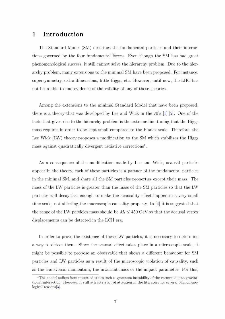
The SM describes the fundamental particles that matter is made of, and how they

interact. The main pillars of matter are fermions, and the force carriers are bosons.

The difference between fermions and bosons is their spins; fermions carry half-integer

spins, and bosons carry integer spins. Fermions are divided into two families, leptons

and quarks, each of which have 6 members with spin 12

(see Figure 1).

Figure 1: The fundamental particles in the Standard Model [5].

8

These building blocks of matter interact with each other through the four funda-

mental forces. Each force has one or more carriers:

Table 1: Fundamental forces in nature known so far.

Force Strength Theory MediatorStrong 10 Chromodynamics Gluon

Electromagnetic 10−2 Electrodynamics PhotonWeak 10−13 Flavordynamics W and Z bosons

Gravitational 10−42 Geometrodynamics Graviton

The SM is simple and powerful. There are complex mathematical expressions that

corroborate the validity of this model and allow theorists to make predictions with

great precision. Over the past five decades, thanks to development of new technology,

almost every theoretically predicted quantity has been successfully measured in parti-

cle physics laboratories. However, the model have some limitations at higher energies.

One of the major problems that the SM faces is that it does not include gravity, which

is one of the four fundamental forces. Also, the SM cannot explain why gravity is

much weaker than the other 3 fundamental forces. Another problem is the wide range

in mass for the elementary particles, e.g., the electron is about 200 times lighter than

the muon and 3500 times lighter than the tau. The same thing happens for quarks. So,

how is it possible to have such a wide spectrum of masses among the building blocks

of matter? Many theorists believe this is unnatural.

Furthermore, the equations of the SM establish relations between the fundamental

particles. For instance, the Higgs boson has a basic mass to which theorists add a

correction for each particle that interact with it, as a result, the heavier the particle,

the larger the correction. Therefore, theorists wonder how the measured Higgs boson

mass can be as small as it was found. In order to solve this riddle, theorists predict

that there might be other yet undiscovered particles that can change this picture, so

that the corrections made to the Higgs mass can be cancelled out by some other hy-

pothetical particle and lead to the low Higgs boson mass that has been measured.

Moreover, the SM only describes visible matter, which is a very small part of what

the Universe is made of. There is ample evidence showing that the Universe is mostly

9

made of dark energy and dark matter. Dark matter is completely different from the

ordinary matter that the SM model describes, so the SM cannot give a complete

picture of what the Universe is made of. Many of these limitations give rise to the

already-mentioned hierarchy problem, which has inspired the proposal of new theories

in Physics Beyond the Standard Model such as: Supersymmetry, Little Higgs, Lee

Wick Standard Model, etc.

3 Lee-Wick Toy Model in QED

Lee and Wick basically studied the possibility that a propagator2 corresponds to

a physical degree of freedom3. In order to briefly illustrate how the Lee-Wick (LW)

theory works, a toy model for a finite theory of Quantum Electrodynamics can be

described considering a one self-interacting scalar field Φ with a higher derivative term

[6], so that its Lagrangian density is4:

Lhd =1

2∂µΦ∂µΦ− 1

2M2(∂2Φ)2 − 1

2m2Φ2 − 1

3!gΦ3 , (1)

the propagator of Φ is:

D(p) =i

p2 − p4/M2 −m2. (2)

The higher derivative propagator has two poles, one corresponding to the massless

photon, and the other corresponding to a massive LW-photon. For M � m, this

propagator has poles at p2 ' m2 and also at p2 'M2, hence the propagator describes

more than one degree of freedom. In order to make these new degrees of freedom

2A propagator gives the amplitude for a particle to travel between two spacetime points.3In the LWSM, every field in the minimal SM has a higher derivative kinetic term that introduces

a corresponding massive LW resonance, which are additional free parameters in the theory and mustbe high enough to evade current experimental constraints

4In equation 1, m is the mass of a photon in QED, M is the mass of a LW-photon, and p isthe four-vector momentum of the propagator. The Lagrangian density shown in equation 1 can beexplained as: the first term is the kinetic term; the second term shows the interaction of the particlewith itself; the third term is the potential term; and the fourth is also and interaction term, whichshows that a particle comes in and two particles go out.

10

evident in the theory, an auxiliary scalar field5 Φ is introduced, so that the theory is:

L =1


2m2Φ2 − Φ∂2Φ +

1

2M2Φ2 − 1

3!gΦ3 . (3)

Computing the equation of motion of Φ, one gets:

∂L∂Φ− ∂µ

∂L∂(∂µΦ)

= 0

∂L∂Φ

= −∂2Φ + M2Φ

∂L∂(∂µΦ)

= 0

⇒ −∂2Φ + M2Φ = 0

Φ =∂2Φ

M2,

so by replacing Φ in equation 3, Lhd is obtained.

By defining Φ = Φ + Φ, there are two fields, a normal scalar field Φ which corre-

sponds to our SM toy theory, and a new field Φ, which will be the LW field. As a

result, the Lagrangian is:

L =1


2∂µΦ∂µΦ +

1

2M2Φ2 − 1

2m2(Φ− Φ)2 − 1

3!g(Φ− Φ)3 (4)

For simplicity, the mass m is neglected6, so that the propagator of Φ is given by:

D(p) =−i

p2 −M2. (5)

5The auxiliary LW fields will reproduce the higher derivative terms when integrated out[6].6In the LWSM, the mass M of LW particles must be heavier than the mass m of SM particles, so

m�M .

11

The LW field is associated with a nonpositive definite norm on the Hilbert space, as

seen in D(p). Hence, if this state were to be stable, unitarity of the S matrix 7 would

be violated. However, with a further analysis and by modifying the usual integration

contour in Feynman calculus as was proposed by Lee and Wick, it can be seen that

the width of the LW field differs in sign from the widths of usual particles, and as a

consequence, the unitarity of the theory is maintained. Thus the unusual sign of the

propagator is compensated by the unusual sign of the decay width [6].

This LW prescription is equivalent to imposing the boundary condition that there

are no outgoing exponentially growing modes. Therefore, these conditions cause vi-

olations of causality. As it was previously mentioned, it is believed that the acausal

effects in the LW theory occur only on microscopic scales, and show up as a peculiar

time ordering of events [6], i.e., the decay products of a LW particle appear at times

before the LW particle itself is created; this means that a wrong vertex displacement

is obtained.

After a proton-proton collision, as part of the products of the collision, there are

long-lived particles, which will decay after travelling a certain distance. The proton-

proton interaction point in space is known as the primary vertex (PV), and the point

in space where the long-lived particles decay, is the secondary vertex (SV). A wrong

vertex displacement is a vertex displacement in which the decay products coming from

the secondary vertex have a total momentum that points from the secondary to the

primary vertex [4]. On the other hand, in the case of the usual causal effect, i.e., SM

particles, for long-lived particles, the vertex displacement shows a behaviour where the

total momentum points from the secondary vertex but away from the primary vertex.

Additionally, short-lived causal particles have their decay products momentum coming

from the primary vertex.

7The S matrix is defined as the matrix element of the transition from one asymptotic set of statesto another. By taking the square of the S matrix, we can calculate the transition probabilities.

12

4 The LHC and the CMS Detector

The Large Hadron Collider (LHC) at CERN is the largest and the most energetic

hadron accelerator in the world. It lies at about 175 m underground in a tunnel with

a ring of superconducting magnets of 27 km in circumference, located beneath the

France-Switzerland border near Geneva, Switzerland. The collider tunnel contains two

adjacent parallel beam pipes that intersect at four points, each containing a beam,

which travel in opposite directions around the ring. In these intersection points, seven

detectors have been constructed. The main experiments at LHC are ATLAS, CMS,

ALICE and LHCb [7]. For our purpose we work with simulations of events in the CMS

detector.

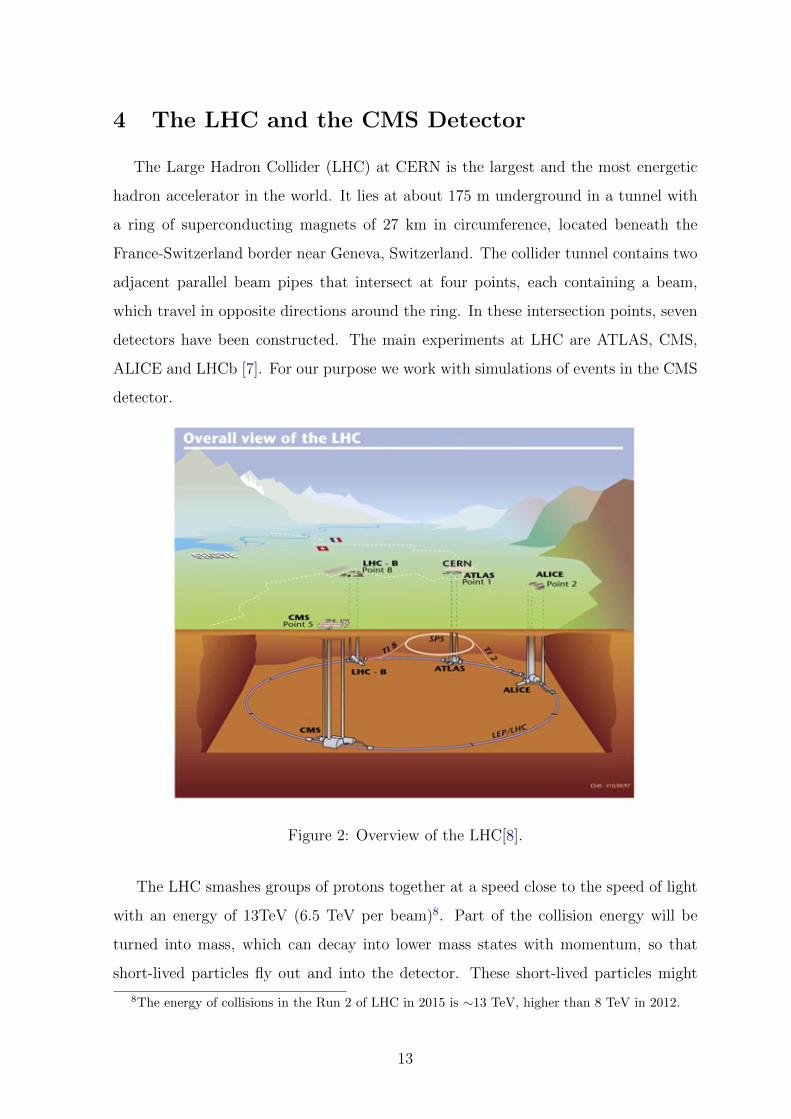
Figure 2: Overview of the LHC[8].

The LHC smashes groups of protons together at a speed close to the speed of light

with an energy of 13TeV (6.5 TeV per beam)8. Part of the collision energy will be

turned into mass, which can decay into lower mass states with momentum, so that

short-lived particles fly out and into the detector. These short-lived particles might

8The energy of collisions in the Run 2 of LHC in 2015 is ∼13 TeV, higher than 8 TeV in 2012.

13

be previously undetected particles, and thus new particles could be observed in the

Compact Muon Solenoid (CMS) particle detector. The new particles that are detected

could give clues about how nature behaves at fundamental level and, as a result, many

theoretical predictions can be confirmed.

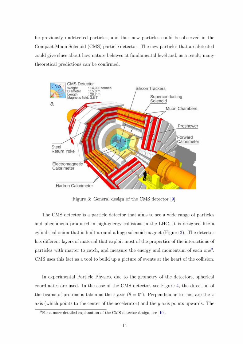
Figure 3: General design of the CMS detector [9].

The CMS detector is a particle detector that aims to see a wide range of particles

and phenomena produced in high-energy collisions in the LHC. It is designed like a

cylindrical onion that is built around a huge solenoid magnet (Figure 3). The detector

has different layers of material that exploit most of the properties of the interactions of

particles with matter to catch, and measure the energy and momentum of each one9.

CMS uses this fact as a tool to build up a picture of events at the heart of the collision.

In experimental Particle Physics, due to the geometry of the detectors, spherical

coordinates are used. In the case of the CMS detector, see Figure 4, the direction of

the beams of protons is taken as the z-axis (θ = 0◦). Perpendicular to this, are the x

axis (which points to the center of the accelerator) and the y axis points upwards. The

9For a more detailed explanation of the CMS detector design, see [10].

14

azimuthal angle, φ, lies in the transverse plane xy. The polar angle θ is replaced by a

quantity known as the pseudorapidity, η, which is defined as:

η = − ln ( tanθ

2) .

Figure 4: Coordinate system used in the CMS detector [11]. The z−axis is the directionof the beams.

Our analysis is based on the characteristics of the LHC in the Run 2. In the Run

2, the LHC collides protons at√s = 13 ∼ 14 TeV 10, with an instantaneous luminosity

L ∼ 1 · 1034 cm−2s−1, and bunch spacing of mostly 25 ns, so that the integrated

luminosity∫L dt is at ∼75−100 fb−1[12].

5 Events generation and selection

For the LW and background events generation, hadronization and detection simu-

lations, MadGraph [13], Pythia 6.420 [14] and Delphes 3.2.0 [15] are used respectively.

For the LW and background events simulation, the run card of MadGraph is modified

so that only events with |η| < 2.4 are generated11. This condition is set in order to

10s is a Mandelstam variable that encodes the energy, momentum, and angles of particles in ascattering process and is generally used in Particle Physics since it is Lorentz-invariant.

11As seen in section 4, due to the design of the CMS detector, particles coming as products ofproton-proton collisions will be localized mainly at the center of the detector, i.e., the particles with

15

ensure that the reconstructed jets come from hard collisions in CMS.

For the hadronization process held in Pythia, no modifications are made to the

default run card. Furthermore, effects like pile-up are not considered. The interac-

tion of decay products with the material in the CMS detector (Run 2) is simulated in

Delphes. In MadGraph, the default run card works with the CMS detector parame-

ters for Delphes, and no special conditions are needed for the hadronization process

in Pythia. Hence, Delphes and Pythia are run along with MadGraph instead of stan-

dalone, so that the events12 are generated for each process with LHC collisions at 13

TeV.

5.1 Lee Wick Events Generation

At first, the process that was intended to be generated is13:

qq → A,Z, B, W 3 → lee lee ,

where, in turn,

lee lee → Ze+Ze− → e+e−jjjj . (6)

However, this process requires to create a new model in MadGraph.

A model for the LWSM in MadGraph was created in [4]. In this model, the mass

term is changed in the range of Ml ≤ 450 GeV. Nevertheless, the events generated

with this model only show the LW particles invariant mass14 resonance and not the

acausal behaviour of the LW particles. Additionally, in [4], the simulations made did

not include the whole simulation chain, i.e., no simulations at the detector level were

made. Thus, it is not be possible to use this model for simulations and to compare

harder transverse momentum will be located at ∼ |η| < 2.4. Particles out of that area are neglectedfrom the analysis since they could be part of pile-up events.

12The normalized events in each process depend on the cross section obtained with MadGraph foreach process.

13Where q is a quark and q is an antiquark; A, Z, B, W 3 are gauge bosons; and lee and lee are LWleptons and antileptons respectively.

14See section 6.2.

16

them with real data obtained from CMS.

Since the only parameter that changes in the LW partners of each SM particle is

the mass, an analogue process to the one shown above was simulated:

qq → Z Z → jjjj . (7)

If the electron and positron from equation (6) were included as part of the decay

products in our process in equation (7), they will enhance the available handles for

detection, i.e., the process in equation (7) is harder to analyse than the one in equation

(6) would be.

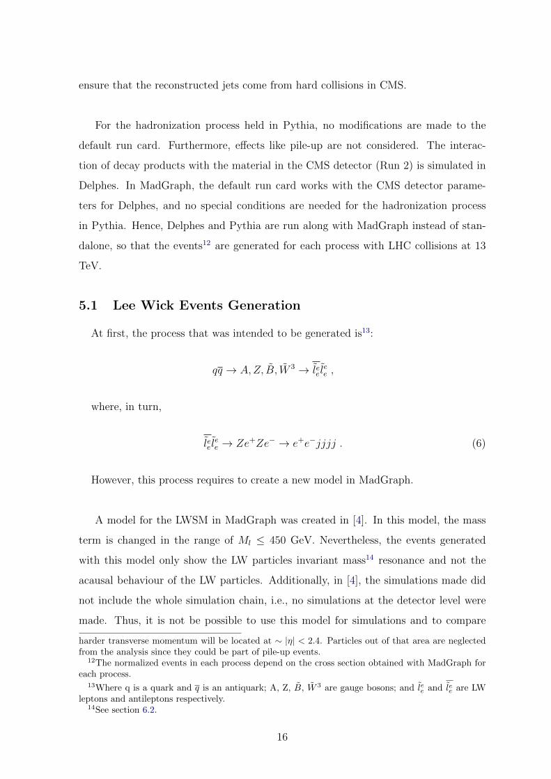
Figure 5: Feynman diagram for a LW process with LW-leptons simulated in MadGraph.The process generated was the one shown in equation (7) but with a mass of 300 GeV.

The process shown in equation (7), Figure 5, is chosen since it is similar to the

process we are intending to simulate in equation (6). In the LWSM theory, the LW

particles decay into SM particles so fast that it is not possible to observe them, but

their effects could be detected in the CMS detector. As a result, simulating a SM

process with heavier gauge bosons, 300 GeV, that decay into 4 jets, would give us LW

events as long as the vertex displacement and momentum is also modified to reproduce

the acausal effect.

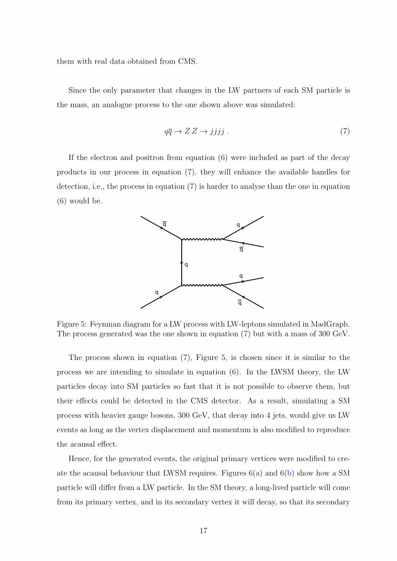
Hence, for the generated events, the original primary vertices were modified to cre-

ate the acausal behaviour that LWSM requires. Figures 6(a) and 6(b) show how a SM

particle will differ from a LW particle. In the SM theory, a long-lived particle will come

from its primary vertex, and in its secondary vertex it will decay, so that its secondary

17

(a) (b)

Figure 6: Vertex displacements and total momentum for causal and acausal particles.Primary (PV) and secondary (SV) vertices are shown for a (a) SM particle and a (b)LW particle.

vertex and the center of mass of its products have a total momentum with the same

direction as the total momentum of the particle in its primary vertex. On the other

hand, a LW particle will have a secondary vertex and its products with a center of

mass total momentum in opposite direction to the total momentum of the particle in

its primary vertex.

For the process shown in equation (7), 20000 events15 with an energy of 13TeV were

generated. In order to obtain a better approximation for the LW process, the Z boson

mass was modified in the parameters card of MadGraph, so that the new mass is 300

GeV with a total cross section16 of 66.7 fb [4].

Figure 7 shows a 3D view of a SM event in the CMS detector generated in MadGraph

with equation (7), and Figures 8 and 9 show a φ - and longitudinal-view, respectively,

of the same SM event in the detector before the modification to have a wrong vertex

displacement is made. To get both plots, the Event Display option of Delphes was used,

which is an Event Visualization Environment of the ROOT[16] package. In Figure 7,

it is seen that the number of jets obtained, depicted by the yellow cones, is greater

15The LW events generated had a total cross section of 66.7 fb, and the integrated luminosity that wewill work with is 100 fb−1. As a result, 20000 were generated in order to have a significant normalisedsignal to work with compared to the others, as it will be seen in the Events Analysis section.

16In [4], three LW-leptons are analysed, with 3 different masses: 300, 400 and 500 GeV. The LW-leptons that were chosen for the present analysis are the ones with mass of 300 GeV because theirtotal cross section is the largest among those three cases.

18

Figure 7: 3D view of an acausal event in the parametrized CMS detector for the LWprocess in equation (7) without modifications to get the acausal behaviour. The yellowcones represent the reconstructed jets, the blue lines are the particles tracks, and theblue and red rectangles are deposits of energy in the calorimeters.

Figure 8: φ−view of an acausal event in the parametrized CMS detector for the LWprocess in equation (7) without modifications to get the acausal behaviour. The yellowtriangles represent the reconstructed jets, the blue lines are the particles tracks, andthe blue and red rectangles are deposits of energy in the calorimeters.

19

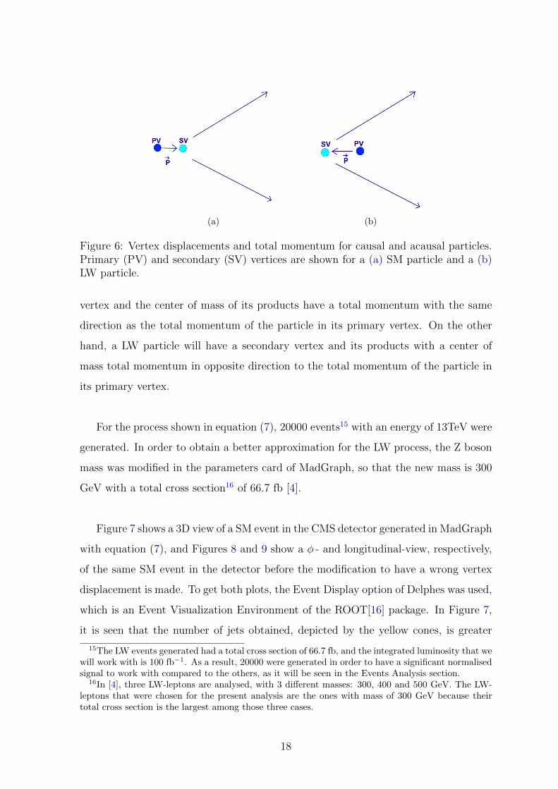
Figure 9: Longitudinal view of an acausal event in the parametrized CMS detector forthe LW process in equation (7) without modifications to get the acausal behaviour.Theyellow triangles represent the reconstructed jets and the blue lines are the particlestracks.

than the one that was initially generated with the run card at MadGraph. Also, in

Figures 7 and 8, one notices that there are 4 jets that form two pairs since they are

not too spatially apart from each other, and that the other 2 jets do not seem to be

spatially connected to each other or to the other jets. As a result, it can be said that

those 2 jets might have been generated from the underlying event17, or are not ener-

getic enough to be part of the main decay products of the process shown in equation (7).

The events obtained had as many as 11 jets, so in order to displace the primary

vertices, it was necessary to first identify the 4 jets that came from the LW particles (Z

bosons in the simulation). To find those 4 jets the following procedure was pursued:

• Since the simulation is made for the CMS detector, only jets with |η| < 2.4 are

considered to come from a LW particle.

• In the detector level simulation, the position coordinates of the jets and LW

17The underlying event is everything except the 4 outgoing hard scattered jets[17]. In real life, thiseffect will be enhanced due to pile up interactions.

20

particles, are zero or near zero, so it is necessary to modify them negligibly in

order to obtain the shortest distance from the LW particle primary vertex to each

jet trajectory. The position coordinates of the jets and LW particles are slightly

modified with a Gaussian distribution18.

• The 4 jets that are considered for the analysis are chosen as the ones that have

the largest transversal momentum in each event. Later, those 4 jets are matched

as a pair that come from the same particle mother by comparing their invariant

mass with the mass of the hypothetical LW particle.

• In order to find the origin of the jets, the center of mass between the pair of jets

that were previously selected is computed with:

−→P CM =

−→P1 P1 +

−→P2 P2

P1 + P2

PTCM=

√P 2XCM

+ P 2YCM

cos φCM

=PXCM

PTCM

(8)

sinh ηCM

=PZCM

PTCM

. (9)

The directions of the center of mass of the jets (in φ and η) are compared to

18Delphes, by default, does not work with primary and secondary vertices. In Delphes, most ofthe collisions occur at the center of the detector, so, mainly all the initial particles are located in theorigin. Also, since the particles that we work with decay really fast, the secondary vertex where thejets originate, are not separated from the particle that originated it. For instance, the Z boson witha half-life of the order of 10−25 s would make a displacement of ∼ 10−18 m. Since this displacementis too small, the data is automatically set to zero instead of a value of the order of 10−18 m. In orderto compute the pseudo impact parameter (see section 6.1), it is necessary to have the jets separatedfrom the particle primary vertex, so that the pseudo impact parameter is not zero. The scale taken isa value taken from the half-life of the particle and the CMS detector efficiency. This value is used togive a smearing to the PV and a point in the jet track. The same principle is used for displacing theprimary vertices and the jets positions in the backgrounds.

21

those of each LW particle with:

∆R =√

(∆φ)2 + (∆η)2 , (10)

the smallest ∆R is used to designate which LW particle produced the pair of jets.

• The LW particle is displaced in the direction of the center of mass of the two

jets that come from it. The displacement is made with a Gaussian distribution

so that it varies between 20 and 50 µm. This displacement was taken since in

[4] the wrong vertex displacements considered for the analysis are greater than

∆x = 20µm, which is consistent with the resolution of the CMS pixel tracker

detector.

• For the analysis, the new total momentum of the displaced LW particle is deter-

mined by computing the total momentum of the center of mass between the 2 jets

that originated from that LW particle. The direction of the new total momentum

is changed to be opposite to the original direction.

After this process19, a wrong displaced vertex is obtained for each LW particle,

which will be used for a further analysis.

5.2 Background Events Generation

For our analysis of the LW process, only three backgrounds are considered: 4

jets production from ZZ, 4 jets production from ZZ with causal displacements, and tt

production. For a more accurate and complete analysis, more backgrounds are needed,

but for simplicity, only three backgrounds are considered; these are representative of

the causal particle that can be encountered in the CMS.

5.2.1 Jets production from ZZ

The first background is the same process as the one done for the LW process in

equation (7), the only difference in the events generation is that the Z boson mass is

19Appendix I shows the script lwevents.C which was used to create a LW process by using the ZZprocess.

22

not modified in the run card of MadGraph.

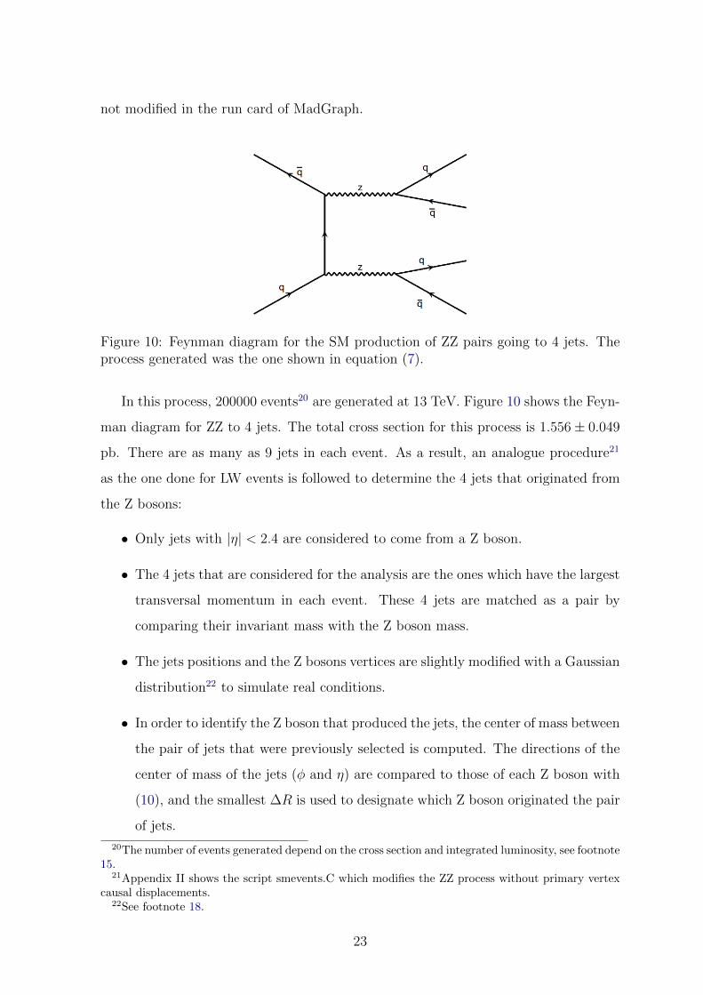
Figure 10: Feynman diagram for the SM production of ZZ pairs going to 4 jets. Theprocess generated was the one shown in equation (7).

In this process, 200000 events20 are generated at 13 TeV. Figure 10 shows the Feyn-

man diagram for ZZ to 4 jets. The total cross section for this process is 1.556± 0.049

pb. There are as many as 9 jets in each event. As a result, an analogue procedure21

as the one done for LW events is followed to determine the 4 jets that originated from

the Z bosons:

• Only jets with |η| < 2.4 are considered to come from a Z boson.

• The 4 jets that are considered for the analysis are the ones which have the largest

transversal momentum in each event. These 4 jets are matched as a pair by

comparing their invariant mass with the Z boson mass.

• The jets positions and the Z bosons vertices are slightly modified with a Gaussian

distribution22 to simulate real conditions.

• In order to identify the Z boson that produced the jets, the center of mass between

the pair of jets that were previously selected is computed. The directions of the

center of mass of the jets (φ and η) are compared to those of each Z boson with

(10), and the smallest ∆R is used to designate which Z boson originated the pair

of jets.

20The number of events generated depend on the cross section and integrated luminosity, see footnote15.

21Appendix II shows the script smevents.C which modifies the ZZ process without primary vertexcausal displacements.

22See footnote 18.

23

• The total momentum of the displaced Z boson is determined by the total mo-

mentum of the center of mass of the pair jets that were originated from it.

5.2.2 Jets production from ZZ with causal displacements

This background is simulated in order to show an hypothetical case representing any

causal process with long-lived particles. For simplicity, the process shown in equation 7

is simulated as in section 5.2.1, with the same number of events and total cross section.

For selecting the jets that we work with in this background, the same procedure as the

one shown in section 5.2.1 is followed. After that, the causal displacement is simulated

with a Gaussian distribution so that the secondary vertex displacement varies between

20 and 50 µm23. This displacement is taken to show the difference between the pseudo

impact parameter of a causal particle, and an acausal particle. The same displacement

as for the LW particles is taken but the direction of the momentum is preserved to

obtain a causal scenario.

5.2.3 tt Production Events Generation

The general tt production24 process considered is,

qq → t t→ bW+ bW− .

However, depending on the decay modes of the W± bosons, 2, 4 or 6 jets can be

obtained. Thus, 4 different processes for tt production are generated at 13 TeV. Figure

11 shows the Feynman diagrams for the different decays of the W± bosons. Table 2

shows the processes that were simulated, and the number of events generated for each

process.

The number of events produced for each process was determined depending on the

branching ratio of the process. In total, 10000 events were generated for tt production.

After the events generation, it is seen that more jets than the expected are obtained,

23Appendix II shows the script smevents.C which modifies the ZZ process with primary vertexcausal displacements.

24The tt production was considered as a background since it has been already widely studied, sotheir behaviour is predictable.

24

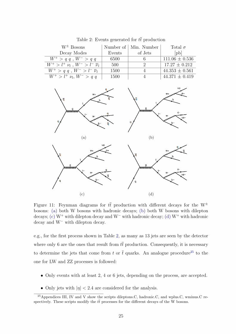
Table 2: Events generated for tt production

W± Bosons Number of Min. Number Total σDecay Modes Events of Jets [pb]

W+ > q q , W− > q q 6500 6 111.06 ± 0.536W+ > l+ νl , W− > l− νl 500 2 17.27 ± 0.212W+ > q q , W− > l− νl 1500 4 44.353 ± 0.561W+ > l+ νl, W

− > q q 1500 4 44.371 ± 0.419

(a) (b)

(c) (d)

Figure 11: Feynman diagrams for tt production with different decays for the W±

bosons: (a) both W bosons with hadronic decays; (b) both W bosons with dileptondecays; (c) W+ with dilepton decay and W− with hadronic decay; (d) W+ with hadronicdecay and W− with dilepton decay.

e.g., for the first process shown in Table 2, as many as 13 jets are seen by the detector

where only 6 are the ones that result from tt production. Consequently, it is necessary

to determine the jets that come from t or t quarks. An analogue procedure25 to the

one for LW and ZZ processes is followed:

• Only events with at least 2, 4 or 6 jets, depending on the process, are accepted.

• Only jets with |η| < 2.4 are considered for the analysis.

25Appendices III, IV and V show the scripts dileptons.C, hadronic.C, and wplus.C, wminus.C re-spectively. These scripts modify the tt processes for the different decays of the W bosons.

25

• The 2, 4 or 6 jets (depending on the process) with hardest transversal momentum

are selected. In order to determine the origin of each of the jets, ∆R is used in

comparison with the t and t quarks.

• The jets position coordinates, t and t quarks vertices are modified infinitesimally

with Gaussian distributions26.

• The coordinates and momentum of the t and t quarks are determined with the

center of mass of the jets that come from them.

6 Events Analysis

After the events selection process, the number of jets, which are used for computing

the invariant mass27 between the two hardest jets and the pseudo impact parameter28

is reduced. For the analysis, an integrated luminosity29 of 100 fb−1 was considered.

Since each process had a different cross section and number of events, it is necessary

to normalize the data generated. Table 3 shows the weight factor30 computed for each

process with:

Wf =σ

N

∫L dt , (11)

where σ is the cross section, L is the integrated luminosity, and N is the number

of events that were originally simulated.

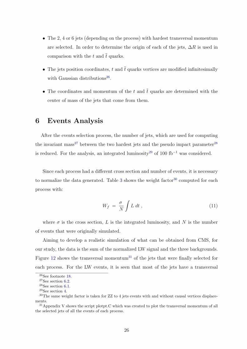
Aiming to develop a realistic simulation of what can be obtained from CMS, for

our study, the data is the sum of the normalized LW signal and the three backgrounds.

Figure 12 shows the transversal momentum31 of the jets that were finally selected for

each process. For the LW events, it is seen that most of the jets have a transversal

26See footnote 18.27See section 6.2.28See section 6.1.29See section 4.30The same weight factor is taken for ZZ to 4 jets events with and without causal vertices displace-

ments.31Appendix V shows the script plotpt.C which was created to plot the transversal momentum of all

the selected jets of all the events of each process.

26

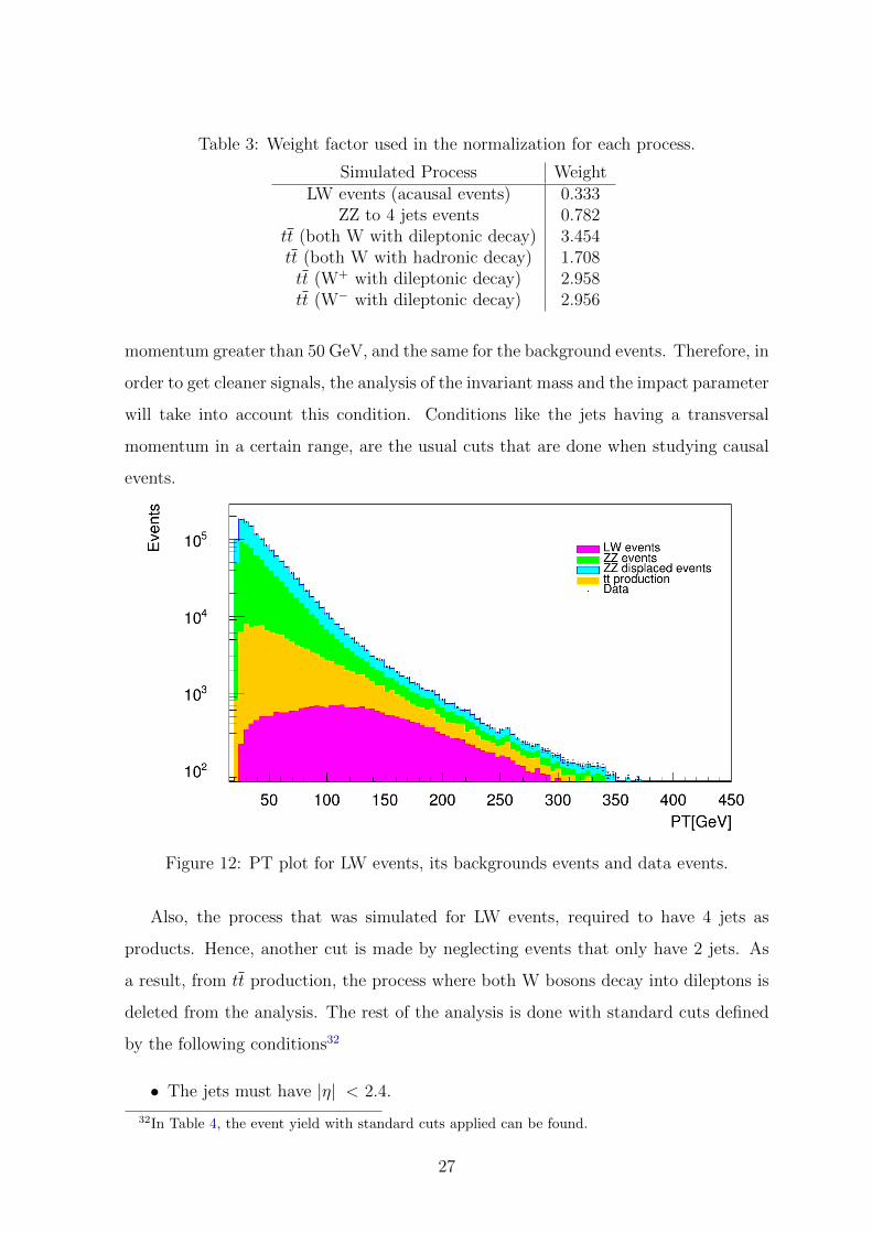
Table 3: Weight factor used in the normalization for each process.

Simulated Process WeightLW events (acausal events) 0.333

ZZ to 4 jets events 0.782tt (both W with dileptonic decay) 3.454tt (both W with hadronic decay) 1.708tt (W+ with dileptonic decay) 2.958tt (W− with dileptonic decay) 2.956

momentum greater than 50 GeV, and the same for the background events. Therefore, in

order to get cleaner signals, the analysis of the invariant mass and the impact parameter

will take into account this condition. Conditions like the jets having a transversal

momentum in a certain range, are the usual cuts that are done when studying causal

events.

Figure 12: PT plot for LW events, its backgrounds events and data events.

Also, the process that was simulated for LW events, required to have 4 jets as

products. Hence, another cut is made by neglecting events that only have 2 jets. As

a result, from tt production, the process where both W bosons decay into dileptons is

deleted from the analysis. The rest of the analysis is done with standard cuts defined

by the following conditions32

• The jets must have |η| < 2.4.

32In Table 4, the event yield with standard cuts applied can be found.

27

• Each event must have at least 4 jets.

• The jets transversal momentum must be greater than 50 GeV.

6.1 Pseudo Impact Parameter

In order to show the acausal behaviour of the LW events, a new variable, the pseudo

impact parameter, is computed. The impact parameter is defined as the distance of

closest approach of a track to the interaction point [18]. However, in this case, we

define a pseudo impact parameter which will be considered as the dot product between

the momentum of the particle mother that originated the jets−→P CM , and the vector

position of the point at which one gets the shortest distance from this particle mother

primary vertex to the track of each jet−→D . The pseudo impact parameter was defined

in that way so that it allows one to notice the effect that the wrong vertex displacement

have in the signal, especially because of the direction of the total linear momentum.

Figure 13: Vector of the shortest distance D from the primary vertex PV to the jetstrajectory

The same analysis procedure is used for the LW and background events. For sim-

plicity, it is assumed that the trajectory followed by the jets is linear. The directions

of the jet η and φ, and the modified jet position coordinates are used in order to de-

termine the linear equation of the jet trajectory. After that, the vector of the shortest

distance between the primary vertex of the particle that produced the jets, and the jet

trajectory is found (Figure 13)33.

33Appendix V shows an analogue structure of the script that was created to plot the pseudo impact

28

It is expected to see a significant change in the pseudo impact parameter−→D ·−→P CM

computed for the LW events and the background events. This is because for the LW

events, the primary vertices were displaced with a greater width than in the back-

grounds, and also, the PV was modified to be a wrong displaced vertex.

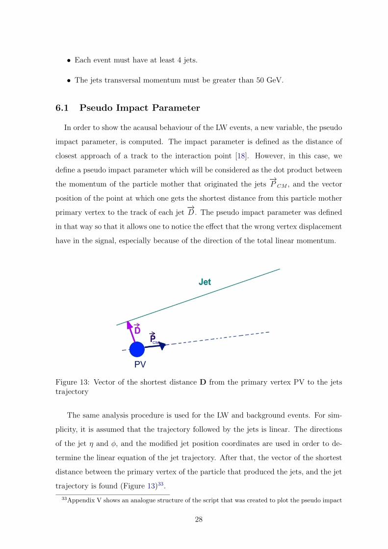
Figures 14, 15, 16 and 17 show the pseudo impact parameters for each process.

Clearly, it can be seen that for three backgrounds, ZZ to 4 jets and tt production,

which are SM processes, the behaviour of the pseudo impact parameter is symmetrical.

On the other hand for the LW process and the ZZ to 4 jets but with causal vertex

displacement, the histograms show an asymmetrical behaviour. Figure 18 shows the

three process together. For these events only the standard cuts have been made.

Figure 14: Pseudo impact parameter for events where ZZ pairs decay into 4 jets withoutprimary vertex displacement. The standard cuts mentioned before are already set.

By analysing the plots, one can infer the fact that due to the asymmetrical be-

haviour and the wrong vertex displacement for LW events, there is a region where the

LW signal predominates. The cut chosen is for−→D ·−→P CM <-10 GeV·mm 34. This cut in

parameter of the different signals that was computed with appendices I, II and III.34The script used for the cut in the pseudo impact parameter, is similar to the one shown in

Appendix V.

29

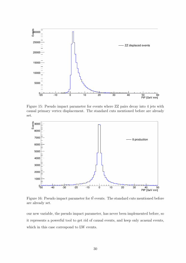
Figure 15: Pseudo impact parameter for events where ZZ pairs decay into 4 jets withcausal primary vertex displacement. The standard cuts mentioned before are alreadyset.

Figure 16: Pseudo impact parameter for tt events. The standard cuts mentioned beforeare already set.

our new variable, the pseudo impact parameter, has never been implemented before, so

it represents a powerful tool to get rid of causal events, and keep only acasual events,

which in this case correspond to LW events.

30

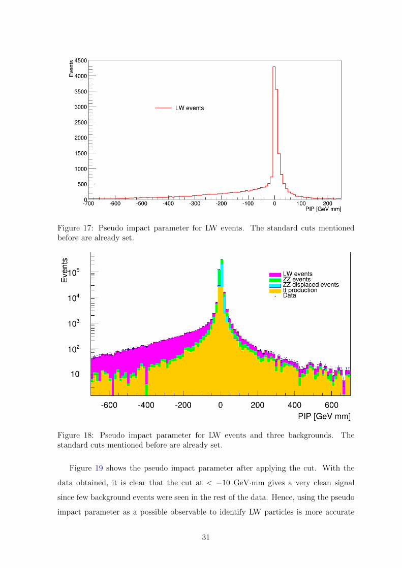
Figure 17: Pseudo impact parameter for LW events. The standard cuts mentionedbefore are already set.

Figure 18: Pseudo impact parameter for LW events and three backgrounds. Thestandard cuts mentioned before are already set.

Figure 19 shows the pseudo impact parameter after applying the cut. With the

data obtained, it is clear that the cut at < −10 GeV·mm gives a very clean signal

since few background events were seen in the rest of the data. Hence, using the pseudo

impact parameter as a possible observable to identify LW particles is more accurate

31

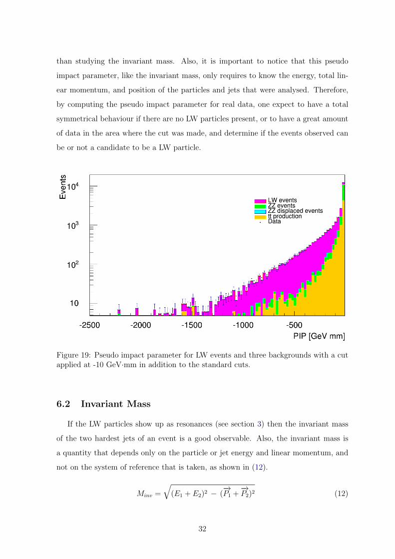
than studying the invariant mass. Also, it is important to notice that this pseudo

impact parameter, like the invariant mass, only requires to know the energy, total lin-

ear momentum, and position of the particles and jets that were analysed. Therefore,

by computing the pseudo impact parameter for real data, one expect to have a total

symmetrical behaviour if there are no LW particles present, or to have a great amount

of data in the area where the cut was made, and determine if the events observed can

be or not a candidate to be a LW particle.

Figure 19: Pseudo impact parameter for LW events and three backgrounds with a cutapplied at -10 GeV·mm in addition to the standard cuts.

6.2 Invariant Mass

If the LW particles show up as resonances (see section 3) then the invariant mass

of the two hardest jets of an event is a good observable. Also, the invariant mass is

a quantity that depends only on the particle or jet energy and linear momentum, and

not on the system of reference that is taken, as shown in (12).

Minv =

√(E1 + E2)2 − (

−→P1 +

−→P2)2 (12)

32

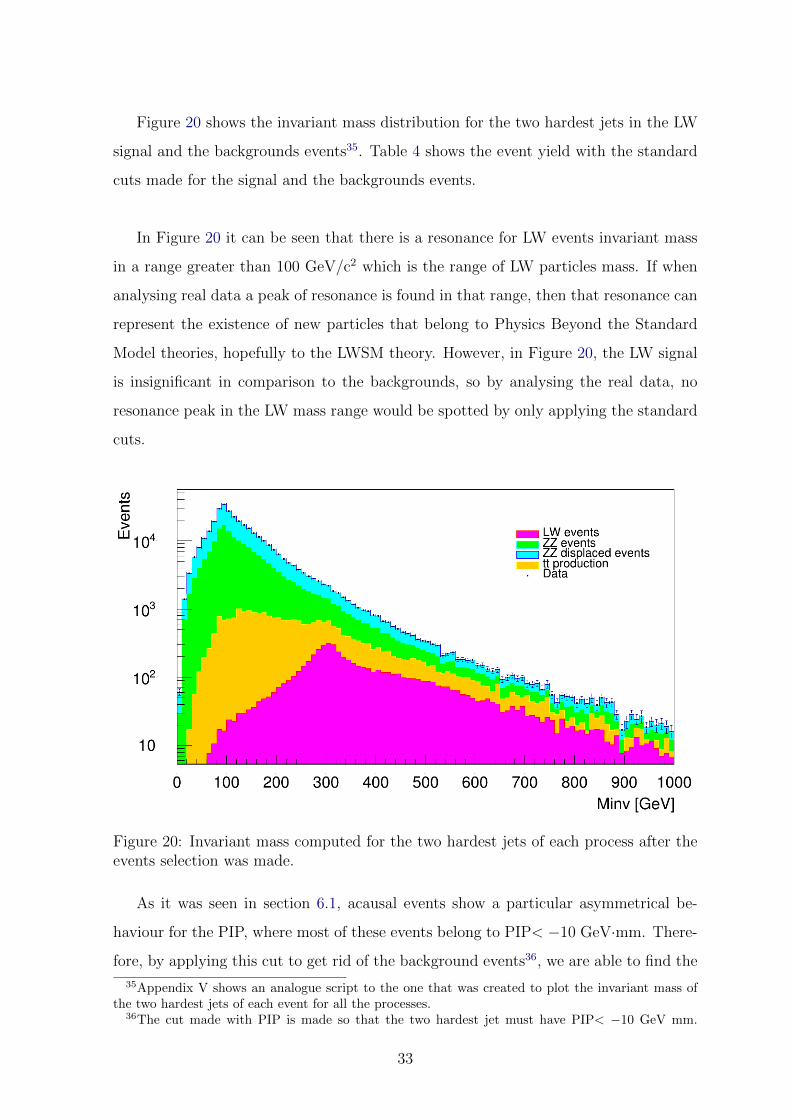
Figure 20 shows the invariant mass distribution for the two hardest jets in the LW

signal and the backgrounds events35. Table 4 shows the event yield with the standard

cuts made for the signal and the backgrounds events.

In Figure 20 it can be seen that there is a resonance for LW events invariant mass

in a range greater than 100 GeV/c2 which is the range of LW particles mass. If when

analysing real data a peak of resonance is found in that range, then that resonance can

represent the existence of new particles that belong to Physics Beyond the Standard

Model theories, hopefully to the LWSM theory. However, in Figure 20, the LW signal

is insignificant in comparison to the backgrounds, so by analysing the real data, no

resonance peak in the LW mass range would be spotted by only applying the standard

cuts.

Figure 20: Invariant mass computed for the two hardest jets of each process after theevents selection was made.

As it was seen in section 6.1, acausal events show a particular asymmetrical be-

haviour for the PIP, where most of these events belong to PIP< −10 GeV·mm. There-

fore, by applying this cut to get rid of the background events36, we are able to find the

35Appendix V shows an analogue script to the one that was created to plot the invariant mass ofthe two hardest jets of each event for all the processes.

36The cut made with PIP is made so that the two hardest jet must have PIP< −10 GeV mm.

33

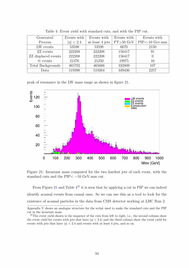
Table 4: Event yield with standard cuts, and with the PIP cut.

Generated Events with Events with Events with Events withProcess |η| < 2.4 at least 4 jets PT>50 GeV PIP<-10 Gev·mm

LW events 53598 53598 6670 2150ZZ events 222208 222208 156417 91

ZZ displaced events 222208 222208 156417 0tt events 21376 21250 19975 16

Total Backgrounds 465792 465666 332809 107Data 519390 519264 339436 2257

peak of resonance in the LW mass range as shown in figure 21.

Figure 21: Invariant mass computed for the two hardest jets of each event, with thestandard cuts and the PIP< −10 GeV·mm cut.

From Figure 21 and Table 437 it is seen that by applying a cut in PIP we can indeed

identify acausal events from causal ones. So we can use this as a tool to look for the

existence of acausal particles in the data from CMS detector working at LHC Run 2.

Appendix V shows an analogue structure for the script used to make the standard cuts and the PIPcut in the invariant mass.

37The event yield shown is the sequence of the cuts from left to right, i.e., the second column showthe event yield for events with jets that have |η| < 2.4; and the third column show the event yield forevents with jets that have |η| < 2.4 and events with at least 4 jets, and so on.

34

7 Conclusions

The Lee Wick Standard Model proposes a partial solution to the hierarchy prob-

lem38. The main feature of the LWSM is the possibility of acausal behaviour for LW

particles. As a result, it was intended to use this feature as a tool to determine a

cut in the data for certain observables such as invariant mass, and a pseudo impact

parameter, which was defined in order to emphasize the wrong vertex displacement

produced from LW particles.

The results show that for the pseudo impact parameter, the difference between SM

particles and LW particles is determinant. For the two SM backgrounds without causal

vertices displacements that were used, it was seen that the pseudo impact parameter

that was computed gives a symmetrical histogram; and in the case of the background

with causal vertices displacements an asymmetrical histogram was obtained with most

of the events at PIP> −10 GeV mm. However, for acausal particles, the pseudo impact

parameter gives an asymmetrical histogram, and most of the data are focused on neg-

ative values, PIP< −10 GeV mm. Therefore, a cut was determined at -10 GeV·m and

thus most of the events that remained belong to the LW signal. The PIP behaviour

that was found is crucial property for the LW process since it shows a relevant cut that

can be used for a further analysis of data coming from the LHC in the Run 2.

Furthermore, the analysis of the invariant mass of the two hardest jets in each

event showed that by only applying the standard cuts it was hard to spot new mass

resonances in the LW mass range, so it would not be feasible to find these acausal

particles with those conditions. Nevertheless, by implementing a new cut that focus

on the acausal behaviour, PIP< −10 GeV mm, we can get rid of background events,

and a resonance in invariant mass could be found in an easier way within the LW mass

range. Hence, the pseudo impact parameter is an important tool to identify acausal

particles at the LHC in the new era.

38The LWSM only leads with quadratic terms produced by the Higgs mass. For instance, it stillhave limitations at the gravitational force problem.

35

8 Future Work

In order to get a more realistic result, it is suggested to add more backgrounds to

the events simulations, for example, QCD. Also, other effects like pile-up and trigger

need to be taken into account in the events selection procedure. However, due to the

high discrimination power of the new cut given by the pseudo impact parameter, an

analyis of real data from the CMS experiment at LHC in the Run 2 can take advantage

of this new cut and look for data that can be identified as acausal particles in the real

world, which could belong to LWSM theory.

References

[1] T. Lee and G. Wick, “Negative metric and the unitarity of the s-matrix,” Nuclear

Physics B, vol. 9, pp. 209–243, Feb 1969.

[2] T. D. Lee and G. C. Wick, “Finite theory of quantum electrodynamics,” Phys.

Rev. D, vol. 2, pp. 1033–1048, Sep 1970.

[3] K. Bhattacharya, Y.-F. Cai, and S. Das, “Lee-wick radiation induced bouncing

universe models,” Phys. Rev. D, vol. 87,, p. 083511, Jan. 2013.

[4] E. Alvarez, L. D. Rold, C. Schat, and A. Szynkman, “Vertex displacements for

acausal particles: Testing the lee-wick standard model at the lhc,” JHEP, Aug.

2009.

[5] A. Purcell, “Go on a particle quest at the first cern webfest,

https://cds.cern.ch/journal/cernbulletin/2012/35/news%20articles/1473657,”

[6] B. Grinstein, D. O’Connell, and M. B. Wise, “The lee-wick standard model,”

Phys.Rev.D, Apr. 2007.

[7] CERN, “The large hadron collider, http://home.cern/topics/large-hadron-

collider,”

[8] WIGNER, “The wigner data centre and the cernwigner project,

http://wigner.mta.hu/wignerdc/index en.php,”

36

[9] L. Taylor, “Cms detector design, http://cms.web.cern.ch/news/cms-detector-

design,”

[10] T. C. Collaboration, S. Chatrchyan, G. Hmayakyan, V. Khachatryan, A. M. Sirun-

yan, W. Adam, T. Bauer, T. Bergauer, H. Bergauer, M. Dragicevic, and et al.,

“The CMS experiment at the CERN LHC,” Journal of Instrumentation, vol. 3,

pp. S08004–S08004, Aug 2008.

[11] T. Lenzi and G. D. Lentdecker, “Development and study of different muon track

reconstruction algorithms for the level-1 trigger for the cms muon upgrade with

gem detectors,” June 2013.

[12] J. Ellis, “The beautiful physics of lhc run 2,” Dec. 2014.

[13] J. Alwall, R. Frederix, S. Frixione, V. Hirschi, F. Maltoni, O. Mattelaer, H. S.

Shao, T. Stelzer, P. Torrielli, and M. Zaro, “The automated computation of tree-

level and next-to-leading order differential cross sections, and their matching to

parton shower simulations,” JHEP, vol. 07(2014)079, p. 07079, May 2014.

[14] T. Sjostrand, S. Mrenna, and P. Skands, “Pythia 6.4 physics and manual,” JHEP,

JHEP 0605:026,2006.

[15] S. Ovyn, X. Rouby, and V. Lemaitre, “Delphes, a framework for fast simulation

of a generic collider experiment,” Mar. 2009.

[16] R. Brun and F. Rademakers, “Root - an object oriented data analysis framework,”

Nuclear Instruments and Methods in Physics Research Section A: Accelerators,

Spectrometers, Detectors and Associated Equipment, vol. 389, 1997.

[17] R. D. Field, “The underlying event in hard scattering processes,” eConfC,

eConfC010630:P501,2001.

[18] S. Stone, B Decays. World Scientific, 1994.

37

9 Appendices

From the events generation, 6 .root files were obtained, 4 for tt events, 1 for LW

events and 1 for ZZ events. In order to do the events selection, the data stored in

each TTree was analysed by using the MakeClass option from ROOT [16]. MakeClass

generates an .h and a .C files from the .root file. For each TTree, the .h file was only

modified by adding some new functions in the constructor. On the other hand, the .C

file has the all the information about the vertices’ changes, selected transversal mo-

mentum, invariant mass, and pseudo impact parameter. So only the .C files are shown

in appendices I to V.

In appendices VI to IX, there are scripts for the plotting of the LW signal and the

backgrounds. These scripts are based on the data obtained from the files mentioned

above.

9.1 Appendix I: Script for analysing LW acausal particles sig-

nal events.

The following script, lwevents.C, works for LW events. It generates the wrong

vertex displacements, and computes the invariant mass and pseudo impact parameter.

For the pseudo impact parameter it is already considered the fact that only jets with

PT>50 GeV will be analysed.

// Author: Raquel Quishpe

#define lwevents_cxx

#include "lwevents.h"

#include <TH2.h>

#include <TStyle.h>

#include <TCanvas.h>

#include <TRandom.h>

#include "TMath.h"

#include <iostream >

#include <fstream >

using TMath ::ASinH;

using namespace TMath;

38

void lwevents ::data()

{

//The data() function will filter some data , and then displace

//the vertices of the mother particles and the positions of the

//jets that come from it. Since this is a LW process , the mother

// particle ’s vertices are wrongly displaced. The invariant mass

//for the hardest jets is computed. The pseudo impact parameter

//is computed. A cleaner invariant mass is computed.

if (fChain == 0) return;

Long64_t nentries = fChain ->GetEntriesFast ();

Long64_t nbytes = 0, nb = 0;

ofstream myfile1;

ofstream myfile2;

ofstream myfile3;

ofstream myfile4;

ofstream myfile5;

myfile1.open("ip_lw.dat");

myfile2.open("pt_lw.dat");

myfile3.open("im_lw.dat");

myfile4.open("cim_lw.dat");

myfile5.open("cut_ip_lw.dat");

// variables to count the number of jets after every filter

int count4jets =0;

int countip =0;

int countjets =0;

// variables to find the hardest jets and compute the

// invariant mass

float hardpt;

int ID[4];

int Jet_ID [4];

float invmass [6];

float Jet_E [4];

float dminv [6];

//LW particle ’s mass in GeV

39

float lw_mass = 300;

// variables for the PV and jets position and momentum

int Z_ID [4]; //0 from first Z, 1 from second Z

Float_t Z_PT [2];

Float_t Z_Phi [2];

Float_t Z_Eta [2];

Float_t Z_X [2];

Float_t Z_Y [2];

Float_t Z_Z [2];

Float_t LW_X [2];

Float_t LW_Y [2];

Float_t LW_Z [2];

// variables to change and exchange the vertex of the Z

Float_t d_sigma =30e-3; //20um

Float_t sigma=9e-3; //9um

Float_t z_sigma =9e-5;

Float_t Jet_X [4];

Float_t Jet_Y [4];

Float_t Jet_Z [4];

Float_t Small_X [4];

Float_t Small_Y [4];

Float_t Small_Z [4];

Float_t Small_LW_X [4];

Float_t Small_LW_Y [4];

Float_t Small_LW_Z [4];

Float_t fPx [2];

Float_t fPy [2];

Float_t fPz [2];

// variable to determine the impact parameter

Float_t LW_IP [4];

for (Long64_t jentry =0; jentry <nentries;jentry ++) {

Long64_t ientry = LoadTree(jentry);

if (ientry < 0) break;

nb = fChain ->GetEntry(jentry); nbytes += nb;

// if (Cut(ientry) < 0) continue;

for (int ijjet=0 ; ijjet <kMaxJet ; ijjet++ ){

if (Jet_PT[ijjet ]==0) continue;

countjets ++;

40

}

if (Jet_PT [3]==0) continue;

for (int jjjet=0 ; jjjet <kMaxJet ; jjjet++ ){

if (Jet_PT[jjjet ]==0) continue;

count4jets ++;

}

//let’s find the 4 hardest jets

hardpt = 0;

for (int ijet0=0 ; ijet0 <kMaxJet ; ijet0++ ){

if ( fabs(Jet_Eta[ijet0]) >2.4 ) continue;

if(Jet_PT[ijet0]>=hardpt){

hardpt = Jet_PT[ijet0];

ID[0] = ijet0;

}

}

hardpt = 0;



if (ijet1 == ID[0]) continue;



ID[1] = ijet1;

}

}

hardpt = 0;



if ( ijet2==ID[0] || ijet2==ID[1] ) continue;



ID[2] = ijet2;

}

}

hardpt = 0;



if ( ijet3==ID[0] || ijet3==ID[1] || ijet3==ID[2]) continue;


41


ID[3] = ijet3;

}

}

//let’s compute the invariant mass for every combination between the 4

jets

for(int ijet =0; ijet <4; ijet ++){

Jet_E[ijet]= Jet_PT[ID[ijet ]]* Jet_PT[ID[ijet ]]* cosh(Jet_Eta[ID[

ijet ]])*cosh(Jet_Eta[ID[ijet ]]) + Jet_Mass[ID[ijet ]]*

Jet_Mass[ID[ijet ]];

Jet_E[ijet]=sqrt(Jet_E[ijet]);

}

for(int k0=1; k0 <4; k0++){

invmass[k0 -1] = pow( ( Jet_PT[ID [0]]* cos(Jet_Phi[ID [0]]) +

Jet_PT[ID[k0]]* cos(Jet_Phi[ID[k0]]) ) , 2 ) + pow( (

Jet_PT[ID [0]]* sin(Jet_Phi[ID [0]]) + Jet_PT[ID[k0]]* sin(

Jet_Phi[ID[k0]]) ) , 2 ) + pow( ( Jet_PT[ID [0]]* sinh(

Jet_Eta[ID [0]]) + Jet_PT[ID[k0]]* sinh(Jet_Eta[ID[k0]]) ) ,

2 );

invmass[k0 -1] = pow( (Jet_E [0]+ Jet_E[k0]) , 2 ) - invmass[k0

-1];

invmass[k0 -1] = sqrt(invmass[k0 -1]);

dminv[k0 -1] = fabs(invmass[k0 -1]- lw_mass);

}

for(int k1=2; k1 <4; k1++){

invmass[k1+1] = pow( ( Jet_PT[ID [1]]* cos(Jet_Phi[ID [1]]) +





2 );

invmass[k1+1] = pow( (Jet_E [1]+ Jet_E[k1]) , 2 ) - invmass[k1

+1];

invmass[k1+1] = sqrt(invmass[k1+1]);

dminv[k1+1] = fabs(invmass[k1+1]- lw_mass);

}

invmass [5] = pow( ( Jet_PT[ID [2]]* cos(Jet_Phi[ID [2]]) + Jet_PT

[ID[3]]* cos(Jet_Phi[ID[3]]) ) , 2 ) + pow( ( Jet_PT[ID

42

[2]]* sin(Jet_Phi[ID[2]]) + Jet_PT[ID[3]]* sin(Jet_Phi[ID

[3]]) ) , 2 ) + pow( ( Jet_PT[ID[2]]* sinh(Jet_Eta[ID[2]])

+ Jet_PT[ID[3]]* sinh(Jet_Eta[ID[3]]) ) , 2 );

invmass [5] = pow( (Jet_E [2]+ Jet_E [3]) , 2 ) - invmass [5];

invmass [5] = sqrt(invmass [5]);

dminv [5] = fabs(invmass [5]- lw_mass);

//now let’s look for the smallest difference btw the invariant mass

//and the LW particle ’s mass

float s_dm=dminv [0];

int i_dm_1 =0;

for(int im=0; im <6; im++){

if(dminv[im]<=s_dm){

s_dm=dminv[im];

i_dm_1=im;

}

}

if(i_dm_1 ==0) { //

Jet_ID [0]=ID[0] ;

Jet_ID [1]=ID[1] ;

Jet_ID [2]=ID[2] ;

Jet_ID [3]=ID[3] ;

}//

if(i_dm_1 ==1) { //

Jet_ID [0]=ID[0] ;

Jet_ID [1]=ID[2] ;

Jet_ID [2]=ID[1] ;

Jet_ID [3]=ID[3] ;

}//

if(i_dm_1 ==2) { //

Jet_ID [0]=ID[0] ;

Jet_ID [1]=ID[3] ;

Jet_ID [2]=ID[1] ;

Jet_ID [3]=ID[2] ;

}//

if(i_dm_1 ==3) { //

Jet_ID [0]=ID[1] ;

43

Jet_ID [1]=ID[2] ;

Jet_ID [2]=ID[0] ;

Jet_ID [3]=ID[3] ;

}//

if(i_dm_1 ==4) { //

Jet_ID [0]=ID[1] ;

Jet_ID [1]=ID[3] ;

Jet_ID [2]=ID[0] ;

Jet_ID [3]=ID[2] ;

}//

if(i_dm_1 ==5) { //

Jet_ID [0]=ID[2] ;

Jet_ID [1]=ID[3] ;

Jet_ID [2]=ID[1] ;

Jet_ID [3]=ID[0] ;

}//

//let’s select the direction of the Z bosons based on the jets center

of mass

float px, py, pz;

//for the first Z

px = Jet_PT[Jet_ID [0]]* cos(Jet_Phi[Jet_ID [0]]) + Jet_PT[Jet_ID

[1]]* cos(Jet_Phi[Jet_ID [1]]);

py = Jet_PT[Jet_ID [0]]* sin(Jet_Phi[Jet_ID [0]]) + Jet_PT[Jet_ID

[1]]* sin(Jet_Phi[Jet_ID [1]]);

pz = Jet_PT[Jet_ID [0]]* sinh(Jet_Eta[Jet_ID [0]]) + Jet_PT[

Jet_ID [1]]* sinh(Jet_Eta[Jet_ID [1]]);

Z_PT [0] = sqrt( pow(px ,2) + pow(py ,2));

Z_Phi [0] = acos (px/Z_PT [0]);

Z_Eta [0] = ASinH (pz/Z_PT [0]);

//for the second Z









44


//let’s change the jets origin

for(int jeti =0; jeti <4; jeti ++){// ******

Jet_X[jeti] = gRandom -> Gaus(0,sigma);

Jet_Y[jeti] = gRandom -> Gaus(0,sigma);

Jet_Z[jeti] = gRandom -> Gaus(0,sigma);

}//end of jeti

//let’s change a little the vertex for the original model

for(int iz=0; iz <2; iz++){

float SMR;

SMR = gRandom -> Gaus(0,z_sigma);

Z_X[iz] = SMR*cos(Pi()-Z_Phi[iz])*sin(2* atan(exp(-(Pi()-Z_Eta[

iz]))));

Z_Y[iz] = SMR*sin(Pi()-Z_Phi[iz])*sin(2* atan(exp(-(Pi()-Z_Eta[

iz]))));

Z_Z[iz] = SMR*cos (2* atan(exp(-(Pi()-Z_Eta[iz]))));

}

//let’s get the acausal vertex

float d;

float theta;

int aux_mj;

while (d<20e-3){

d = gRandom -> Gaus(0,d_sigma);

}

for(int ia=0; ia <2; ia++){//****

fPx[ia] = d*cos(Z_Phi[ia])*sin(2* atan(exp(-Z_Eta[ia])));

fPy[ia] = d*sin(Z_Phi[ia])*sin(2* atan(exp(-Z_Eta[ia])));

fPz[ia] = d*cos (2* atan(exp(-Z_Eta[ia])));

LW_X[ia]=Z_X[ia]+fPx[ia];

LW_Y[ia]=Z_Y[ia]+fPy[ia];

LW_Z[ia]=Z_Z[ia]+fPz[ia];

}

for(int lwj =0; lwj <4; lwj++){//*****

LW_IP[lwj ]=0;

if(Jet_PT[Jet_ID[lwj ]]<50) continue;// comment for no cut

if(lwj ==0 || lwj ==1) aux_mj =0;

if(lwj ==2 || lwj ==3) aux_mj =1;

theta = 2*atan(exp(-Jet_Eta[Jet_ID[lwj]]));

45

Small_LW_X[lwj] = pow( LW_X[aux_mj] , 2) + pow( LW_Y[aux_mj] ,

2) + pow( LW_Z[aux_mj], 2 ) + LW_Y[aux_mj ]*( Jet_X[lwj]*

tan(Jet_Phi[Jet_ID[lwj]])-Jet_Y[lwj]) + LW_Z[aux_mj ]*(

Jet_X[lwj]/(cos(Jet_Phi[Jet_ID[lwj]])*tan(theta))-Jet_Y[

lwj]);

Small_LW_X[lwj] = Small_LW_X[lwj]/( LW_X[aux_mj ]+LW_Y[aux_mj ]*

tan(Jet_Phi[Jet_ID[lwj]])+LW_Z[aux_mj ]/(cos(Jet_Phi[Jet_ID

[lwj]])*tan(theta)));

Small_LW_Y[lwj] = Jet_Y[lwj] + (Small_LW_X[lwj] - Jet_X[lwj])*

tan(Jet_Phi[Jet_ID[lwj]]);

Small_LW_Z[lwj] = Jet_Z[lwj] + (Small_LW_X[lwj] - Jet_X[lwj])

/(cos(Jet_Phi[Jet_ID[lwj ]])*tan(theta));

LW_IP[lwj] = Small_LW_X[lwj]*( Z_PT[aux_mj ])*cos(Pi()-Z_Phi[

aux_mj ]) + Small_LW_Y[lwj ]*( Z_PT[aux_mj ])*sin(Pi()-Z_Phi[

aux_mj ]) +Small_LW_Z[lwj ]*( Z_PT[aux_mj ])*sinh(Pi()-Z_Eta[

aux_mj ]);

myfile1 <<LW_IP[lwj]<<endl;

countip ++;

}

// applying some cuts and storing some information in .dat

for(int pti =0; pti <4; pti++){

myfile2 <<Jet_PT[Jet_ID[pti]]<<endl;

}

myfile3 <<invmass [0]<<endl;

if(Jet_PT[Jet_ID [0]] >50 && Jet_PT[Jet_ID [1]] >50){


if(LW_IP [0]<=-10 && LW_IP [1] <=-10){


}

}

}//end of jentry

myfile1.close();

myfile2.close();

myfile3.close();

myfile4.close();

myfile5.close();

cout <<"original: "<<countjets <<endl;

cout <<"at least 4 jets: "<<count4jets <<endl;

46

cout <<"after ip: "<<countip <<endl;

}

9.2 Appendix II: Scripts for analysing background events of

ZZ to 4 jet with and without primary vertex displace-

ments.

The following script, smevents.C, works for the ZZ to 4 jets process in the SM. It

computes the invariant mass and impact parameter. For the impact parameter it is

already considered the fact that only jets with PT>50 GeV will be analysed. It also

reproduce the causal vertex displacement that is used for the second background.


#define smevents_cxx

#include "smevents.h"

#include <TH2.h>

#include <TStyle.h>



#include "TMath.h"


#include <fstream >



void smevents ::data()

{

//The data() function will filter some data , and then smear

//the vertices of the mother particles and the positions of the

//jets that come from it.

//The invariant mass for the hardest jets is computed. The pseudo

// impact parameter is computed. A cleaner invariant mass is computed.




ofstream myfile1;

47

ofstream myfile2;

ofstream myfile3;

ofstream myfile4;

ofstream myfile5;

myfile1.open("ip_sm.dat");

myfile2.open("pt_sm.dat");

myfile3.open("im_sm.dat");

myfile4.open("cim_sm.dat");

myfile5.open("cut_ip_sm.dat");


int count4jets =0;

int countip =0;

int countjets =0;


// invariant mass

float hardpt;

int ID[4];

int Jet_ID [4];

float invmass [6];

float Jet_E [4];

float dminv [6];

//Z boson mass in GeV

float Z_mass = 91.1876;


Float_t Z_PT [2];

Float_t Z_Phi [2];

Float_t Z_Eta [2];

Float_t Z_X [2];

Float_t Z_Y [2];

Float_t Z_Z [2];





Float_t Jet_X [4];

Float_t Jet_Y [4];

Float_t Jet_Z [4];


48



// variables to determine the impact parameter

Float_t SM_IP [4];








countjets ++;

}




count4jets ++;

}


hardpt = 0;





ID[0] = ijet0;

}

}

hardpt = 0;






ID[1] = ijet1;

}

}

hardpt = 0;


49





ID[2] = ijet2;

}

}

hardpt = 0;






ID[3] = ijet3;

}

}






}//end of ijet

for(int k0=1; k0 <4; k0++){






2 );


-1];


dminv[k0 -1] = fabs(invmass[k0 -1]- Z_mass);

}

for(int k1=2; k1 <4; k1++){




50



2 );


+1];


dminv[k1+1] = fabs(invmass[k1+1]- Z_mass);

}








dminv [5] = fabs(invmass [5]- Z_mass);

//now let’s look for the smallest one


int i_dm_1 =0;



s_dm=dminv[im];

i_dm_1=im;

}

}

if(i_dm_1 ==0) { //

Jet_ID [0]=ID[0] ;

Jet_ID [1]=ID[1] ;

Jet_ID [2]=ID[2] ;

Jet_ID [3]=ID[3] ;

}//

if(i_dm_1 ==1) { //

Jet_ID [0]=ID[0] ;

Jet_ID [1]=ID[2] ;

Jet_ID [2]=ID[1] ;

Jet_ID [3]=ID[3] ;

}//

if(i_dm_1 ==2) { //

51

Jet_ID [0]=ID[0] ;

Jet_ID [1]=ID[3] ;

Jet_ID [2]=ID[1] ;

Jet_ID [3]=ID[2] ;

}//

if(i_dm_1 ==3) { //

Jet_ID [0]=ID[1] ;

Jet_ID [1]=ID[2] ;

Jet_ID [2]=ID[0] ;

Jet_ID [3]=ID[3] ;

}//

if(i_dm_1 ==4) { //

Jet_ID [0]=ID[1] ;

Jet_ID [1]=ID[3] ;

Jet_ID [2]=ID[0] ;

Jet_ID [3]=ID[2] ;

}//

if(i_dm_1 ==5) { //

Jet_ID [0]=ID[2] ;

Jet_ID [1]=ID[3] ;

Jet_ID [2]=ID[1] ;

Jet_ID [3]=ID[0] ;

}//


of mass

float px, py, pz;

//for the first Z










//for the second Z

52















}//end of jeti



float SMR;



iz]))));


iz]))));


}

//let’s find the vector for the shortest distance and IP in the

original model SM

float theta;

int aux_mj;

for(int mj=0; mj <4; mj++){

SM_IP[mj]=0;

if(mj==0 || mj==1) aux_mj =0;

if(mj==2 || mj==3) aux_mj =1;

if(Jet_PT[Jet_ID[mj]]<50) continue;// comment for no cut

theta = 2*atan(exp(-Jet_Eta[Jet_ID[mj]]));

Small_X[mj] = pow( Z_X[aux_mj] , 2) + pow( Z_Y[aux_mj] , 2) +

pow( Z_Z[aux_mj], 2 ) + Z_Y[aux_mj ]*( Jet_X[mj]*tan(Jet_Phi

[Jet_ID[mj]])-Jet_Y[mj]) + Z_Z[aux_mj ]*( Jet_X[mj]/(cos(

53

Jet_Phi[Jet_ID[mj]])*tan(theta))-Jet_Y[mj]);

Small_X[mj] = Small_X[mj]/( Z_X[aux_mj ]+Z_Y[aux_mj ]*tan(Jet_Phi

[Jet_ID[mj]])+Z_Z[aux_mj ]/(cos(Jet_Phi[Jet_ID[mj]])*tan(

theta)));

Small_Y[mj] = Jet_Y[mj] + (Small_X[mj] - Jet_X[mj])*tan(

Jet_Phi[Jet_ID[mj]]);

Small_Z[mj] = Jet_Z[mj] + (Small_X[mj] - Jet_X[mj])/(cos(

Jet_Phi[Jet_ID[mj]])*tan(theta));

SM_IP[mj] = Small_X[mj]*Z_PT[aux_mj ]*cos(Z_Phi[aux_mj ]) +

Small_Y[mj]*Z_PT[aux_mj ]*sin(Z_Phi[aux_mj ]) +Small_Z[mj]*

Z_PT[aux_mj ]*sinh(Z_Eta[aux_mj ]);

myfile1 <<SM_IP[mj]<<endl;

countip ++;

}

// applying some cuts and storing some information in .dat



}




if(SM_IP [0]<=-10 && SM_IP [1] <=-10){


}

}

}//end of jentry

myfile1.close();

myfile2.close();

myfile3.close();

myfile4.close();

myfile5.close();




}

/* ************************************************************ */

void smevents :: causal ()

54

{

//The causal () function will filter some data , and then

//give the mother particles vertices a causal displace displacement

//after giving smearing the vertices of the mother particles and

//the positions of the jets that come from it.

//The invariant mass for the hardest jets is computed. The pseudo

// impact parameter is computed. A cleaner invariant mass is computed.




ofstream myfile1;

ofstream myfile2;

ofstream myfile3;

ofstream myfile4;

ofstream myfile5;

myfile1.open("ip_causal.dat");

myfile2.open("pt_causal.dat");

myfile3.open("im_causal.dat");

myfile4.open("cim_causal.dat");

myfile5.open("cut_ip_causal.dat");


int count4jets =0;

int countip =0;

int countjets =0;


// invariant mass

float hardpt;

int ID[4];

int Jet_ID [4];

float invmass [6];

float Jet_E [4];

float dminv [6];

//Z boson mass in GeV

float Z_mass = 91.1876;


Float_t Z_PT [2];

Float_t Z_Phi [2];

55

Float_t Z_Eta [2];

Float_t Z_X [2];

Float_t Z_Y [2];

Float_t Z_Z [2];

Float_t fPx [2];

Float_t fPy [2];

Float_t fPz [2];





Float_t Jet_X [4];

Float_t Jet_Y [4];

Float_t Jet_Z [4];




// variables to determine the impact parameter

Float_t SM_IP [4];








countjets ++;

}




count4jets ++;

}


hardpt = 0;




56


ID[0] = ijet0;

}

}

hardpt = 0;






ID[1] = ijet1;

}

}

hardpt = 0;






ID[2] = ijet2;

}

}

hardpt = 0;






ID[3] = ijet3;

}

}






}//end of ijet

for(int k0=1; k0 <4; k0++){

57






2 );


-1];


dminv[k0 -1] = fabs(invmass[k0 -1]- Z_mass);

}

for(int k1=2; k1 <4; k1++){






2 );


+1];


dminv[k1+1] = fabs(invmass[k1+1]- Z_mass);

}








dminv [5] = fabs(invmass [5]- Z_mass);

//now let’s look for the smallest one


int i_dm_1 =0;



s_dm=dminv[im];

i_dm_1=im;

58

}

}

if(i_dm_1 ==0) { //

Jet_ID [0]=ID[0] ;

Jet_ID [1]=ID[1] ;

Jet_ID [2]=ID[2] ;

Jet_ID [3]=ID[3] ;

}//

if(i_dm_1 ==1) { //

Jet_ID [0]=ID[0] ;

Jet_ID [1]=ID[2] ;

Jet_ID [2]=ID[1] ;

Jet_ID [3]=ID[3] ;

}//

if(i_dm_1 ==2) { //

Jet_ID [0]=ID[0] ;

Jet_ID [1]=ID[3] ;

Jet_ID [2]=ID[1] ;

Jet_ID [3]=ID[2] ;

}//

if(i_dm_1 ==3) { //

Jet_ID [0]=ID[1] ;

Jet_ID [1]=ID[2] ;

Jet_ID [2]=ID[0] ;

Jet_ID [3]=ID[3] ;

}//

if(i_dm_1 ==4) { //

Jet_ID [0]=ID[1] ;

Jet_ID [1]=ID[3] ;

Jet_ID [2]=ID[0] ;

Jet_ID [3]=ID[2] ;

}//

if(i_dm_1 ==5) { //

Jet_ID [0]=ID[2] ;

Jet_ID [1]=ID[3] ;

Jet_ID [2]=ID[1] ;

Jet_ID [3]=ID[0] ;

}//

59


of mass

float px, py, pz;

//for the first Z










//for the second Z















}//end of jeti



float SMR;



iz]))));


iz]))));


60

}

//let’s find the vector for the shortest distance and IP in the

original model SM

float theta;

int aux_mj;

float d;

while (d<20e-3){

d = gRandom -> Gaus(0,d_sigma);

}

for(int ia=0; ia <2; ia++){//****

fPx[ia] = d*cos(Z_Phi[ia])*sin(2* atan(exp(-Z_Eta[ia])));

fPy[ia] = d*sin(Z_Phi[ia])*sin(2* atan(exp(-Z_Eta[ia])));

fPz[ia] = d*cos (2* atan(exp(-Z_Eta[ia])));

Z_X[ia]=Z_X[ia]+fPx[ia];

Z_Y[ia]=Z_Y[ia]+fPy[ia];

Z_Z[ia]=Z_Z[ia]+fPz[ia];

}

for(int mj=0; mj <4; mj++){

SM_IP[mj]=0;

if(mj==0 || mj==1) aux_mj =0;

if(mj==2 || mj==3) aux_mj =1;

if(Jet_PT[Jet_ID[mj]]<50) continue;// comment for no cut

theta = 2*atan(exp(-Jet_Eta[Jet_ID[mj]]));

Small_X[mj] = pow( Z_X[aux_mj] , 2) + pow( Z_Y[aux_mj] , 2) +

pow( Z_Z[aux_mj], 2 ) + Z_Y[aux_mj ]*( Jet_X[mj]*tan(Jet_Phi

[Jet_ID[mj]])-Jet_Y[mj]) + Z_Z[aux_mj ]*( Jet_X[mj]/(cos(

Jet_Phi[Jet_ID[mj]])*tan(theta))-Jet_Y[mj]);

Small_X[mj] = Small_X[mj]/( Z_X[aux_mj ]+Z_Y[aux_mj ]*tan(Jet_Phi

[Jet_ID[mj]])+Z_Z[aux_mj ]/(cos(Jet_Phi[Jet_ID[mj]])*tan(

theta)));

Small_Y[mj] = Jet_Y[mj] + (Small_X[mj] - Jet_X[mj])*tan(

Jet_Phi[Jet_ID[mj]]);

Small_Z[mj] = Jet_Z[mj] + (Small_X[mj] - Jet_X[mj])/(cos(

Jet_Phi[Jet_ID[mj]])*tan(theta));

SM_IP[mj] = Small_X[mj]*Z_PT[aux_mj ]*cos(Z_Phi[aux_mj ]) +

Small_Y[mj]*Z_PT[aux_mj ]*sin(Z_Phi[aux_mj ]) +Small_Z[mj]*

Z_PT[aux_mj ]*sinh(Z_Eta[aux_mj ]);

myfile1 <<SM_IP[mj]<<endl;

61

countip ++;

}



}




if(SM_IP [0]<=-10 && SM_IP [1] <=-10){


}

}

}//end of jentry

myfile1.close();

myfile2.close();

myfile3.close();

myfile4.close();

myfile5.close();




}

9.3 Appendix III: Scripts for analysing tt production back-

ground events.

The following script, dileptons.C, works for tt events where the W bosons from the

process only decay to dileptons.


#define dileptons_cxx

#include "dileptons.h"

#include <TH2.h>

#include <TStyle.h>




#include <fstream >

62

#include "TMath.h"



using namespace std;

void dileptons ::pt()

{




float hardpt =0;

Int_t ID[2];

ofstream myfile1;

ofstream myfile2;

ofstream myfile3;

myfile1.open("pt_dileptons.dat");

myfile2.open("im_dileptons.dat");

myfile3.open("cim_dileptons.dat");






//only accept events that have at least 2 jets

if(Jet_PT [1]==0) continue;

// finding the 2 hardest jets

hardpt =0;

for(int j0=0; j0 <kMaxJet; j0++){

if (Jet_PT[j0 ]==0) continue;

if (fabs(Jet_Eta[j0]) >2.4) continue;

if (fabs(Jet_PT[j0]) >=hardpt){

hardpt = fabs(Jet_PT[j0]);

ID[0] = j0;

}

}

hardpt =0;


if (j1==ID[0]) continue;

63





ID[1] = j1;

}

}

for(int k=0; k<2; k++){

myfile1 <<Jet_PT[ID[k]]<<endl;

}

float hardinvm;

float jete1 , jete2;

jete1 = sqrt( pow( Jet_Mass[ID[0]] ,2 ) + pow( Jet_PT[ID[0]]* cosh(

Jet_Eta[ID [0]]) ,2 ) );

jete2 = sqrt( pow( Jet_Mass[ID[1]] ,2 ) + pow( Jet_PT[ID[1]]* cosh(

Jet_Eta[ID [1]]) ,2 ) );

hardinvm = sqrt( pow( jete1+jete2 ,2 ) - pow(( Jet_PT[ID[0]]* cos(

Jet_Phi[ID [0]])+Jet_PT[ID [1]]* cos(Jet_Phi[ID [1]])) ,2) - pow((

Jet_PT[ID[0]]* sin(Jet_Phi[ID [0]])+Jet_PT[ID [1]]* sin(Jet_Phi[ID

[1]])),2 ) - pow(( Jet_PT[ID[0]]* sinh(Jet_Eta[ID[0]])+Jet_PT[ID

[1]]* sinh(Jet_Eta[ID[1]])) ,2) );

myfile2 <<hardinvm <<endl;

if(Jet_PT[ID[0]] >50 || Jet_PT[ID[1]] >50){

myfile3 <<hardinvm <<endl;

}

}//end of nentries

myfile1.close();

myfile2.close();

myfile3.close();

}// end of pt()

// ******************************************************

void dileptons :: iparameter ()

{




float hardpt =0;

64

Int_t ID[2];

int countip =0;

int countjet =0;

int count2j =0;

float drt [4];

float aux_drt;

int aux_id;

int id[2];

float sx ,sy ,sz,ip,theta;

float x,y,z;

float vx ,vy ,vz;

Float_t j_sigma =9e-3; //9um for the jet component

Float_t t_sigma =9e-5;//for the t vertex

ofstream myfile;

myfile.open("ip_dileptons.dat");






for(int a=0; a<kMaxJet; a++){

countjet ++;

}

//only accept events that have at least 2 jets

if(Jet_PT [1]==0) continue;

for(int b=0; b<kMaxJet; b++){

count2j ++;

}

// finding the 2 hardest jets

hardpt =0;






ID[0] = j0;

}

}

65

hardpt =0;


if (j1==ID[0]) continue;





ID[1] = j1;

}

}

// setting the mother particle

for(int kj=0; kj <2; kj++){

drt[kj] = sqrt ( pow( (Jet_Phi[ID[kj]]- Particle_Phi [6]) , 2

) + pow( (Jet_Eta[ID[kj]]- Particle_Eta [6]) , 2 ) );

drt[kj+2] = sqrt ( pow( (Jet_Phi[ID[kj]]- Particle_Phi [7]) , 2

) + pow( (Jet_Eta[ID[kj]]- Particle_Eta [7]) , 2 ) );

}

aux_drt = drt [0];

for(int kn=0; kn <2; kn++){

if(drt[kn]<=aux_drt){

aux_drt = drt[kn];

aux_id = kn;

}

}

if ( aux_id ==0 || aux_id ==3 ){

id [0]=6;

id [1]=7;

}

if ( aux_id ==1 || aux_id ==2 ){

id [0]=7;

id [1]=6;

}

// displacing the vertices and computing ip

for(int k=0; k<2; k++){

x = gRandom ->Gaus(0,j_sigma);

y = gRandom ->Gaus(0,j_sigma);

z = gRandom ->Gaus(0,j_sigma);

vx = gRandom ->Gaus(0,t_sigma);

66

vy = gRandom ->Gaus(0,t_sigma);

vz = gRandom ->Gaus(0,t_sigma);

theta = 2*atan(exp(-Jet_Eta[ID[k]]));

sx = (vx*vx + vy*vy + vz*vz + vy*(x*tan(Jet_Phi[ID[k]])-y) +

vz*(x/(cos(Jet_Phi[ID[k]])*tan(theta))-z))/(vx + vy*tan(

theta) + vz/(cos(Jet_Phi[ID[k]])*tan(theta)));

sy = y + (sx -x)*tan(Jet_Phi[ID[k]]);

sz = z + (sx -x)/(cos(Jet_Phi[ID[k]])*tan(theta));

ip = sx*Particle_PT[id[k]]* cos(Particle_Phi[id[k]]) + sy*

Particle_PT[id[k]]* sin(Particle_PT[id[k]]) + sz*

Particle_PT[id[k]]* sinh(Particle_Eta[id[k]]);

myfile <<ip <<endl;

countip ++;

}

}//end of nentries

myfile.close();

cout <<"original: "<<countjet <<endl;

cout <<"after at least 2 jets: "<<count2j <<endl;


}// end of iparameter ()

void dileptons :: borrar ()

{





int countsm =0;






int aux=0;

67

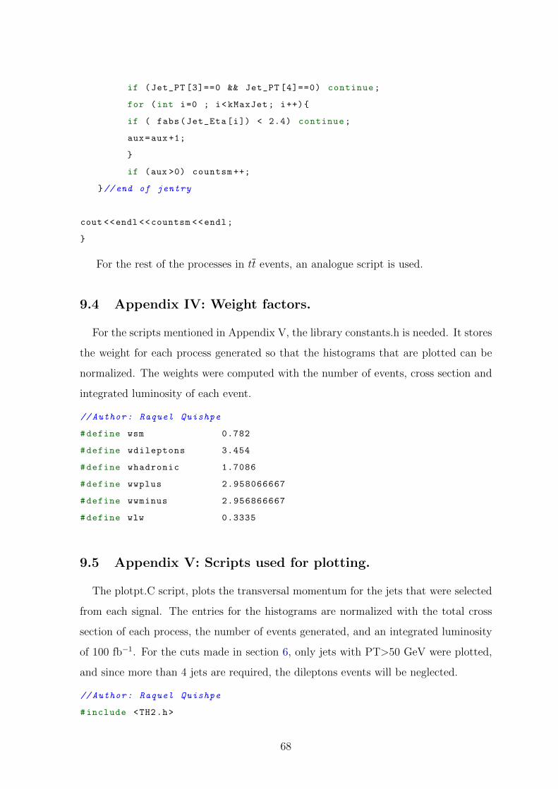
if (Jet_PT [3]==0 && Jet_PT [4]==0) continue;

for (int i=0 ; i<kMaxJet; i++){

if ( fabs(Jet_Eta[i]) < 2.4) continue;

aux=aux +1;

}

if (aux >0) countsm ++;

}//end of jentry

cout <<endl <<countsm <<endl;

}

For the rest of the processes in tt events, an analogue script is used.

9.4 Appendix IV: Weight factors.

For the scripts mentioned in Appendix V, the library constants.h is needed. It stores

the weight for each process generated so that the histograms that are plotted can be

normalized. The weights were computed with the number of events, cross section and

integrated luminosity of each event.


#define wsm 0.782

#define wdileptons 3.454

#define whadronic 1.7086

#define wwplus 2.958066667

#define wwminus 2.956866667

#define wlw 0.3335

9.5 Appendix V: Scripts used for plotting.

The plotpt.C script, plots the transversal momentum for the jets that were selected

from each signal. The entries for the histograms are normalized with the total cross

section of each process, the number of events generated, and an integrated luminosity

of 100 fb−1. For the cuts made in section 6, only jets with PT>50 GeV were plotted,

and since more than 4 jets are required, the dileptons events will be neglected.


#include <TH2.h>

68

#include <TStyle.h>


#include <constants.h>

#include <THStack.h>

void plotpt ()

{

// constructors for the plots

TCanvas *c1 = new TCanvas("c1","c1" ,600,400);

TH1F *h_data = new TH1F("h_data","h_data" ,100, 15, 450);

TH1F *h_SM_pt = new TH1F("h_SM_pt","h_SM_pt" ,100, 15, 450);

TH1F *h_LW_pt = new TH1F("h_LW_pt","h_LW_pt" ,100, 15, 450);

TH1F *h_tt_pt = new TH1F("h_tt_pt","h_tt_pt" ,100, 15, 450);

TH1F *h_causal_pt = new TH1F("h_causal_pt","h_causal_pt" ,100, 15,

450);

THStack *hs = new THStack("hs"," ");

h_data ->Sumw2();

//for ttbar events

//for dileptons

TFile *f1dil = new TFile("dileptons_events.root","RECREATE");

TTree *diltree = new TTree("dileptons_events","ptpact parameter data

for ttbar dileptons");

Long64_t dillines = diltree ->ReadFile("pt_dileptons.dat","ptdileptons"

);

Float_t ptdileptons;

diltree ->SetBranchAddress("ptdileptons",&ptdileptons);

Int_t dilentries = diltree ->GetEntriesFast ();

for(Int_t dilentry =0; dilentry <dilentries; dilentry ++){

diltree ->GetEntry(dilentry);

if (ptdileptons ==0) continue;

h_data ->Fill(ptdileptons ,wdileptons);

h_tt_pt ->Fill(ptdileptons ,wdileptons);

}

//for hadronic decay

TFile *f1had = new TFile("hadronic_events.root","RECREATE");

TTree *hadtree = new TTree("hadronic_events","ptpact parameter data

for ttbar hadronic");

69

Long64_t hadlines = hadtree ->ReadFile("pt_hadronic.dat","pthadronic");

Float_t pthadronic;

hadtree ->SetBranchAddress("pthadronic",&pthadronic);

Int_t hadentries = hadtree ->GetEntriesFast ();

for(Int_t hadentry =0; hadentry <hadentries; hadentry ++){

hadtree ->GetEntry(hadentry);

if(pthadronic ==0) continue;

h_data ->Fill(pthadronic ,whadronic);

h_tt_pt ->Fill(pthadronic ,whadronic);

}

//for wplus to leptons

TFile *f1wplus = new TFile("wplus_events.root","RECREATE");

TTree *wplustree = new TTree("wplus_events","ptpact parameter data for

ttbar wplus");

Long64_t wpluslines = wplustree ->ReadFile("pt_wplus.dat","ptwplus");

Float_t ptwplus;

wplustree ->SetBranchAddress("ptwplus",&ptwplus);

Int_t wplusentries = wplustree ->GetEntriesFast ();

for(Int_t wplusentry =0; wplusentry <wplusentries; wplusentry ++){

wplustree ->GetEntry(wplusentry);

h_data ->Fill(ptwplus ,wwplus);

h_tt_pt ->Fill(ptwplus ,wwplus);

}

//for wminus to leptons

TFile *f1wminus = new TFile("wminus_events.root","RECREATE");

TTree *wminustree = new TTree("wminus_events","ptpact parameter data

for ttbar wminus");

Long64_t wminuslines = wminustree ->ReadFile("pt_wminus.dat","ptwminus"

);

Float_t ptwminus;

wminustree ->SetBranchAddress("ptwminus" ,&ptwminus);

Int_t wminusentries = wminustree ->GetEntriesFast ();

for(Int_t wminusentry =0; wminusentry <wminusentries; wminusentry ++){

wminustree ->GetEntry(wminusentry);

if (ptwminus ==0) continue;

h_data ->Fill(ptwminus ,wwminus);

h_tt_pt ->Fill(ptwminus ,wwminus);

}

70

// ************************************

//for SM

TFile *f2 = new TFile("sm_events.root","RECREATE");

TTree *smtree = new TTree("sm_events","ptpact parameter data for SM");

Long64_t mlines = smtree ->ReadFile("pt_sm.dat","ptsm");

Float_t ptsm;

smtree ->SetBranchAddress("ptsm",&ptsm);

Int_t smentries = smtree ->GetEntriesFast ();

for(Int_t smentry =0; smentry <smentries; smentry ++){

smtree ->GetEntry(smentry);

if (ptsm ==0) continue;

h_data ->Fill(ptsm ,wsm);

h_SM_pt ->Fill(ptsm ,wsm);

}

//for SM causal

TFile *f2 = new TFile("causal_events.root","RECREATE");

TTree *causaltree = new TTree("causal_events","ptpact parameter data

for casual");

Long64_t mlines = causaltree ->ReadFile("pt_causal.dat","ptcausal");

Float_t ptcausal;

causaltree ->SetBranchAddress("ptcausal" ,&ptcausal);

Int_t causalentries = causaltree ->GetEntriesFast ();

for(Int_t causalentry =0; causalentry <causalentries; causalentry ++){

causaltree ->GetEntry(causalentry);

if (ptcausal ==0) continue;

h_data ->Fill(ptcausal ,wsm);

h_causal_pt ->Fill(ptcausal ,wsm);

}

//for LW

TFile *f3 = new TFile("lw_events.root","RECREATE");

TTree *lwtree = new TTree("lw_events","ptpact parameter data for LW");

Long64_t wlines = lwtree ->ReadFile("pt_lw.dat","ptlw");

Float_t ptlw;

lwtree ->SetBranchAddress("ptlw",&ptlw);

Int_t lwentries = lwtree ->GetEntriesFast ();

for(Int_t lwentry =0; lwentry <lwentries; lwentry ++){

lwtree ->GetEntry(lwentry);

if (ptlw ==0) continue;

71

h_data ->Fill(ptlw ,wlw);

h_LW_pt ->Fill(ptlw ,wlw);

}

TStyle *MyStyle = new TStyle("MyStyle","My Root Styles");

MyStyle ->SetStatColor (0);

MyStyle ->SetCanvasColor (0);

MyStyle ->SetPadColor (0);

MyStyle ->SetPadBorderMode (0);

MyStyle ->SetCanvasBorderMode (0);

MyStyle ->SetFrameBorderMode (0);

MyStyle ->SetOptStat (0);

MyStyle ->SetStatBorderSize (2);

MyStyle ->SetOptTitle (0);

MyStyle ->SetPadTickX (1);

MyStyle ->SetPadTickY (1);

MyStyle ->SetPadBorderSize (2);

MyStyle ->SetPalette (51, 0);

MyStyle ->SetPadBottomMargin (0.15);

MyStyle ->SetPadTopMargin (0.05);

MyStyle ->SetPadLeftMargin (0.15);

MyStyle ->SetPadRightMargin (0.25);

MyStyle ->SetTitleColor (1);

MyStyle ->SetTitleFillColor (0);

MyStyle ->SetTitleFontSize (0.05);

MyStyle ->SetTitleBorderSize (0);

MyStyle ->SetLineWidth (1);

MyStyle ->SetHistLineWidth (3);

MyStyle ->SetLegendBorderSize (0);

MyStyle ->SetNdivisions (502, "x");

MyStyle ->SetMarkerSize (0.8);

MyStyle ->SetTickLength (0.03);

MyStyle ->SetTitleOffset (1.5, "x");

MyStyle ->SetTitleOffset (1.5, "y");

MyStyle ->SetTitleOffset (1.0, "z");

MyStyle ->SetLabelSize (0.05 , "x");

MyStyle ->SetLabelSize (0.05 , "y");

MyStyle ->SetLabelSize (0.05 , "z");

MyStyle ->SetLabelOffset (0.03 , "x");

72

MyStyle ->SetLabelOffset (0.03 , "y");

MyStyle ->SetLabelOffset (0.03 , "z");

MyStyle ->SetTitleSize (0.05 , "x");

MyStyle ->SetTitleSize (0.05 , "y");

MyStyle ->SetTitleSize (0.05 , "z");

gROOT ->SetStyle("MyStyle");

h_LW_pt ->SetLineColor(kRed);

h_LW_pt ->SetFillColor(kMagenta);

h_LW_pt ->SetLineWidth (1);

h_LW_pt ->SetTitle ();

h_SM_pt ->SetLineColor(kCyan);

h_SM_pt ->SetFillColor(kGreen);

h_SM_pt ->SetLineWidth (1);

h_SM_pt ->SetTitle ();

h_tt_pt ->SetLineColor(kYellow);

h_tt_pt ->SetFillColor(kOrange);

h_tt_pt ->SetLineWidth (1);

h_tt_pt ->SetTitle ();

h_causal_pt ->SetLineColor(kBlue);

h_causal_pt ->SetFillColor(kCyan);

h_causal_pt ->SetLineWidth (1);

h_causal_pt ->SetTitle ();

h_data ->SetMarkerColor(kBlack);

h_data ->SetMarkerStyle (7);

h_data ->SetTitle ();

h_data ->GetYaxis ()->SetTitle("Events");

h_data ->GetXaxis ()->SetTitle("PT [GeV]");

hs->Add(h_LW_pt ,"sames");

hs->Add(h_tt_pt ,"sames");

hs->Add(h_SM_pt ,"sames");

hs->Add(h_causal_pt ,"sames");

c1->cd();

hs->Draw();

hs->GetXaxis ()->SetTitle("PT[GeV]");

hs->GetYaxis ()->SetTitle("Events");

hs->GetXaxis ()->SetNdivisions (510);

c1->Modify ();

h_data ->Draw("E1 sames P");

73

c1->Update ();

gPad ->SetLogy ();

leg = new TLegend (0.9 ,0.7 ,0.7 ,0.85);

leg ->SetFillStyle (1001);

leg ->SetFillColor(kWhite);

leg ->SetLineColor(kWhite);

leg ->SetLineWidth (2);

leg ->SetTextFont (42);

leg ->SetTextSize (0.038);

leg ->AddEntry("h_LW_pt","LW events","f");

leg ->AddEntry("h_SM_pt","ZZ events","f");

leg ->AddEntry("h_causal_pt","ZZ displaced events","f");

leg ->AddEntry("h_tt_pt","tt production","f");

leg ->AddEntry("h_data","Data","*P");

leg ->Draw("sames");

c1->Print("jetsPT.png");

cout <<"ttbar:"<<h_tt_pt ->Integral (0 ,10000) <<endl;

cout <<"LW:"<<h_LW_pt ->Integral (0 ,10000) <<endl;

cout <<"SM:"<<h_SM_pt ->Integral (0 ,10000) <<endl;

cout <<"causal:"<<h_causal_pt ->Integral (0 ,10000) <<endl;

cout <<"data:"<<h_data ->Integral (0 ,10000) <<endl;

}//end of plotpt ()

For the rest of the plots, i.e., invariant mass and pseudo impact parameter, a similar

script was used.

74

Date post:	07-Sep-2019
Category:	Documents
Upload:	others
View:	2 times
Download:	0 times

UNIVERSIDAD SAN FRANCISCO DE QUITO -...

Documents