UNIVERSIDADE DE SÃO PAULO Instituto de Ciências Matemáticas e de Computação ISSN 0103-2577 _______________________________ NON-AUTONOMOUS DISSIPATIVE SEMIDYNAMICAL SYSTEMS WITH IMPULSES E. M. BONOTTO D. P. DEMUNER N o 419 _______________________________ NOTAS DO ICMC SÉRIE MATEMÁTICA São Carlos – SP Jan./2016
Transcript
UNIVERSIDADE DE SÃO PAULO Instituto de Ciências Matemáticas e de Computação ISSN 0103-2577
In this paper, we describe the theory of non-autonomous dissipative semidyna-mical systems with impulses. We define the concept of a non-autonomous impulsivesemidynamical system and we study its topological properties. For dissipativitysystems we present results which deal with orbital stability, asymptotic stabilityand stability in the sense of Lyapunov-Barbashin. Also, we present some resultsthat give conditions for a non-autonomous dissipative impulsive system to admit aglobal attractor. Finally, we show that systems of impulsive differential equationsadmit a non-autonomous impulsive semidynamical system associated.
1 Introduction
In the last years, the theory of impulsive systems has been studied and developed inten-sively. This theory is very important since complex problems can be modeled by systemswith impulse conditions. The reader may find some important results and applications in[2, 3, 4], [12, 15] and [21, 22, 23], for instance.
Recently, the theory of dissipative impulsive semidynamical systems has started itsstudy. In [7], we define several types of dissipativity as point, compact, local and bounded.We define the center of Levinson for compact dissipative impulsive semidynamical sys-tems and we study its topological properties. Also, we present results giving necessaryand sufficient conditions to obtain dissipativity. In [8], we define some types of attrac-tors and we study some results which relate the concepts of attractors and dissipativesystems (point, bounded and compact). The theory of dissipative systems for continuousdynamical systems may be found in [9].
In this paper we develop the theory of non-autonomous dissipative semidynamicalsystems with impulses as in the sense of Cheban [9]. In the next lines, we describe theorganization of the paper and the main results.
∗Supported by FAPESP 2010/08994-7 and FAPESP 2012/16709-6.
1
In Section 2, we present the basis of the theory of impulsive semidynamical systemsas basic definitions and notations.
Section 3 deals with the continuity of a function which describes the times of meetingimpulsive sets.
In Section 4, we present additional useful definitions about autonomous dissipativesystems.
Section 5 concerns the main results. We divide this section in three subsections. InSubsection 5.1, we create the theory of non-autonomous semidynamical systems withimpulses. For these systems, we present the concept of dissipativity and we define someconcepts of stability as orbital stability, asymptotic stability and stability in the senseof Lyapunov-Barbashin. Also, we define the center of Levinson for a non-autonomousdissipative compact impulsive semidynamical system and we prove that this center isglobally asymptotically stable and globally asymptotically stable in the sense of Lyapunov-Barbashin provided this center satisfies a special condition.
In Subsection 5.2, we show some results which give necessary and sufficient conditionsfor a non-autonomous impulsive system to admit a global attractor.
Finally, in Subsection 5.3, we consider an impulsive differential equation with impulseeffects at variable times,
u′ = f(t, u),I : M → Rn, (1.1)
where f ∈ C(R × Rn,Rn), M ⊂ Rn is an impulsive set, I is an impulse function andwe show that system (1.1) admits a non-autonomous impulsive semidynamical systemassociated.
2 Preliminaries
Let X be a metric space and R+ be the set of non-negative real numbers. The triple(X, π,R+) is called a semidynamical system, if the function π : X×R+ → X is continuouswith π(x, 0) = x and π(π(x, t), s) = π(x, t + s) for all x ∈ X and t, s ∈ R+. We denotesuch system simply by (X, π). For every x ∈ X, we consider the continuous functionπx : R+ → X given by πx(t) = π(x, t) and we call it the motion of x.
Let (X, π) be a semidynamical system. Given x ∈ X, the positive orbit of x is givenby π+(x) = π(x, t) : t ∈ R+. Given A ⊂ X and ∆ ⊂ [0,+∞), we define
π+(A) =⋃x∈A
π+(x) and π(A,∆) =⋃
x∈A, t∈∆
π(x, t).
For t ≥ 0 and x ∈ X, we define F (x, t) = y ∈ X : π(y, t) = x and, for ∆ ⊂ [0,+∞)and D ⊂ X, we define F (D,∆) = ∪F (x, t) : x ∈ D and t ∈ ∆. Then a point x ∈ X iscalled an initial point if F (x, t) = ∅ for all t > 0.
2
Now we define the concept of semidynamical systems with impulse action. An impul-sive semidynamical system (X, π;MX , IX) consists of a semidynamical system, (X, π), anonempty closed subset MX of X such that for every x ∈ MX there exists εx > 0 suchthat
F (x, (0, εx)) ∩MX = ∅ and π(x, (0, εx)) ∩MX = ∅,and a continuous function IX : MX → X whose action we explain below in the descriptionof the impulsive trajectory of an impulsive system. The set MX is called the impulsiveset and the function IX is called the impulse function. We also define
M+(x) =
(⋃t>0
π(x, t)
)∩MX .
Let (X, π;MX , IX) be an impulsive semidynamical system. We define the functionφX : X → (0,+∞] by
φX(x) =
s, if π(x, s) ∈MX and π(x, t) /∈MX for 0 < t < s,
+∞, if M+(x) = ∅.
This means that φX(x) is the least positive time for which the trajectory of x meets MX
when M+(x) 6= ∅. Thus for each x ∈ X, we call π (x, φX(x)) the impulsive point of x.The impulsive trajectory of x in (X, π;MX , IX) is an X−valued function πx defined
on the subset [0, s) of R+ (s may be +∞). The description of such trajectory followsinductively as described in the following lines.
If M+(x) = ∅, then πx(t) = π(x, t) for all t ∈ R+ and φX(x) = +∞. However, ifM+(x) 6= ∅, there is the smallest positive number s0 such that π(x, s0) = x1 ∈ MX andπ(x, t) /∈MX for 0 < t < s0. Then we define πx on [0, s0] by
πx(t) =
π(x, t), 0 ≤ t < s0
x+1 , t = s0,
where x+1 = IX(x1) and φX(x) = s0. Let us denote x by x+
0 .Since s0 < +∞, the process now continues from x+
1 onwards. If M+(x+1 ) = ∅, then we
define πx(t) = π(x+1 , t − s0) for s0 ≤ t < +∞ and φX(x+
1 ) = +∞. When M+(x+1 ) 6= ∅,
there is the smallest positive number s1 such that π(x+1 , s1) = x2 ∈MX and π(x+
1 , t−s0) /∈MX for s0 < t < s0 + s1. Then we define πx on [s0, s0 + s1] by
πx(t) =
π(x+
1 , t− s0), s0 ≤ t < s0 + s1
x+2 , t = s0 + s1,
where x+2 = IX(x2) and φX(x+
1 ) = s1, and so on. Notice that πx is defined on eachinterval [tn, tn+1], where t0 = 0 and tn+1 =
∑ni=0 si for n = 0, 1, 2, . . .. Hence πx is defined
on [0, tn+1].
3
The process above ends after a finite number of steps, whenever M+(x+n ) = ∅ for some
n. However, it continues infinitely if M+(x+n ) 6= ∅, n = 0, 1, 2, . . . , and in this case the
function πx is defined in the interval [0, T (x)), where T (x) =∑∞
i=0 si.Let (X, π;MX , IX) be an impulsive semidynamical system. Given x ∈ X, the impulsive
positive orbit of x is defined by the set
π+(x) = π(x, t) : t ∈ [0, T (x)).
Analogously to the non-impulsive case, an impulsive semidynamical system satisfiesthe following standard properties: π(x, 0) = x for all x ∈ X and π(π(x, t), s) = π(x, t+ s)for all x ∈ X and for all t, s ∈ [0, T (x)) such that t + s ∈ [0, T (x)). See [6] for a proof ofit.
Given A ⊂ X and t ≥ 0, we define π+(A) =⋃x∈A
π+(x) and π(A, t) =⋃x∈A
π(x, t).
If π+(A) ⊂ A, we say that A is positively π−invariant. And, we say that A is minimalin (X, π;MX , IX) if A = π+(x) for all x ∈ A \MX , see [18].
In all this paper, for each x ∈ X, the motion π(x, t) will be defined for every t ≥ 0,that is, [0,+∞) denotes the maximal interval of definition of πx.
For details about the structure of these types of impulsive semidynamical systems, thereader may consult [5, 6, 7, 8], [10, 11], [13, 14] and [17, 18, 19].
3 Continuity of φX
Let (X, π) be a semidynamical system. Any closed set S ⊂ X containing x (x ∈ X)is called a section or a λ-section through x, with λ > 0, if there exists a closed set L ⊂ Xsuch that
(a) F (L, λ) = S;
(b) F (L, [0, 2λ]) is a neighborhood of x;
(c) F (L, µ) ∩ F (L, ν) = ∅, for 0 ≤ µ < ν ≤ 2λ.
The set F (L, [0, 2λ]) is called a tube or a λ-tube and the set L is called a bar. Let(X, π;MX , IX) be an impulsive semidynamical system. We now present the conditionsTC and STC for a tube.
Any tube F (L, [0, 2λ]) given by a section S through x ∈ X such that S ⊂ MX ∩F (L, [0, 2λ]) is called TC−tube on x. We say that a point x ∈ MX fulfills the TubeCondition and we write (TC), if there exists a TC−tube F (L, [0, 2λ]) through x. Inparticular, if S = MX ∩ F (L, [0, 2λ]) we have a STC−tube on x and we say that a pointx ∈MX fulfills the Strong Tube Condition (we write (STC)), if there exists a STC−tubeF (L, [0, 2λ]) through x.
The following theorem concerns the continuity of φX which is accomplished outsideMX for MX satisfying the condition TC. See [10, Theorem 3.8].
4
Theorem 3.1. Consider an impulsive semidynamical system (X, π;MX , IX). Assumethat no initial point in (X, π) belongs to the impulsive set MX and that each element ofMX satisfies the condition (TC). Then φX is continuous at x if and only if x /∈MX .
4 Additional definitions
Let us consider a metric space X with metric ρX . By BX(x, δ) we mean the openball with center at x ∈ X and radius δ > 0. Given A ⊂ X, let BX(A, δ) = x ∈ X :ρX(x,A) < δ where ρX(x,A) = infρX(x, y) : y ∈ A.
Given A and B nonempty bounded subsets of X, we denote by βX(A,B) the semi-deviation of A to B, that is, βX(A,B) = supρX(a,B) : a ∈ A. The Hausdorff distanceof A to B is given by
dH(A,B) = max
supa∈A
infb∈B
ρX(a, b), supb∈B
infa∈A
ρX(a, b)
.
Let (X, π; MX , IX) be an impulsive semidynamical system and A ⊂ X. The limit setof A ⊂ X in (X, π;MX , IX) is given by
L+X(A) = y ∈ X : there exist sequences xnn≥1 ⊂ A and tnn≥1 ⊂ R+
such that tnn→+∞−→ +∞ and π(xn, tn)
n→+∞−→ y
and the prolongation set of A ⊂ X is defined by
D+X(A) = y ∈ X : there are sequences xnn≥1 ⊂ X and tnn≥1 ⊂ R+ such that
ρX(xn, A)n→+∞−→ 0 and π(xn, tn)
n→+∞−→ y.
If A = x, we set L+X(x) = L+
X(x) and D+X(x) = D+
X(x).
The stable manifold of a set A ⊂ X in (X, π;MX , IX) is defined by
W sX(A) = x ∈ X : lim
t→+∞ρX(π(x, t), A) = 0.
A set A in (X, π;MX , IX) is said to be:
1. orbitally π−stable, if given ε > 0 there is δ = δ(ε) > 0 such that ρX(x,A) < δimplies ρX(π(x, t), A) < ε for all t ≥ 0;
2. π−attracting, if there exists γ > 0 such that BX(A, γ) ⊂ W sX(A);
3. asymptotically π−stable, if it is orbitally π−stable and π−attracting;
5
4. globally asymptotically π−stable, if it is asymptotically π−stable and W sX(A) = X;
5. uniform π−attracting, if there is γ > 0 such that limt→+∞
supx∈BX(A,γ)
ρX(π(x, t), A) = 0.
An impulsive system (X, π;MX , IX) is said to be:
6. point dissipative, if there exists a bounded subset K ⊂ X \MX such that for everyx ∈ X the convergence
limt→+∞
ρX(π(x, t), K) = 0 (4.1)
holds;
7. compact dissipative, if the convergence (4.1) takes place uniformly with respect tox on the compact subsets from X;
8. locally dissipative, if for any point x ∈ X there exists δx > 0 such that the conver-gence (4.1) takes place uniformly with respect to y ∈ BX(x, δx);
9. bounded dissipative, if the convergence (4.1) takes place uniformly with respect to xon every bounded subset from X.
Remark 4.1. IfK is compact in the above definition, the impulsive system (X, π;MX , IX)will be called k−dissipative.
Let (X, π;MX , IX) be compact k−dissipative and K be a nonempty compact set suchthat K ∩MX = ∅ and it is an attractor for all compact subsets of X. The set
J := L+X(K) = ∩π(K, t) : t ≥ 0
is called the center of Levinson of the compact k−dissipative system (X, π;MX , IX). Thereader may find properties of the center of Levinson in [7], see Theorem 3.1 for instance.
The next definition presents several concepts established in [8].
Definition 4.1. An impulsive semidynamical system (X, π;MX , IX):
a) satisfies the condition of Ladyzhenskaya, if for every bounded set B ⊂ X there existsa nonempty compact set KB ⊂ X, KB ∩MX = ∅, such that lim
t→+∞βX(π(B, t), KB) =
0;
b) is called π−asymptotically compact, if for every bounded positively π−invariant setB ⊂ X there exists a nonempty compact KB ⊂ X with KB ∩MX = ∅ such thatlimt→+∞
βX(π(B, t), KB) = 0;
c) is called completely continuous if for every bounded subset B ⊂ X there existl = l(B) > 0 such that π(B, l) is relatively compact and π(B, l) ∩MX = ∅;
6
d) is called weakly b−dissipative if there exist a nonempty bounded set B0 ⊂ X suchthat π+(x) ∩ B0 6= ∅ for every point x from X. In this case we will call B0 thebounded weak b−attractor of (X, π;MX , IX);
e) is called weakly k−dissipative if there exist a nonempty compact set K0 ⊂ X suchthat for every ε > 0 and x ∈ X there is τ = τ(x, ε) > 0 for which π(x, τ) ∈BX(K0, ε). In this case we will call K0 the compact weak k−attractor of(X, π;MX , IX).
The theory of dissipative systems in the continuous case can be found in [9].
5 The main results
In this section we present the main results of the paper. We divide this section in threesubsections. In Subsection 5.1, we construct the theory of non-autonomous dissipativesemidynamical systems with impulses and we study the theory of stability for these sys-tems. In Subsection 5.2, we define the concept of global attractor for a non-autonomousdissipative impulsive semidynamical system and we present conditions for this kind ofsystem to admit a global attractor. In the last subsection, we show that non-autonomoussystems of impulsive differential equations admit a non-autonomous semidynamical sys-tem with impulses associated.
Throughout this section we shall consider the following conditions for the impulsivesemidynamical system (X, π; MX , IX):
(H1) No initial point in (X, π) belongs to the impulsive set MX and each element ofMX satisfies the condition (STC), consequently φX is continuous on X \MX (seeTheorem 3.1).
(H2) MX ∩ IX(MX) = ∅.
Conditions (H1)-(H2) are motivated by several results in the theory of impulsive sys-tems which can be found, in particular, in [7, 8].
5.1 Non-autonomous semidynamical systems with impulses
In [9], the author defines the concept of non-autonomous dissipative dynamical systemsand he presents a systematic study of topological properties for these systems. In thissection, we construct this theory for impulsive semidynamical systems.
Let (X, π;MX , IX) and (Y, σ;MY , IY ) be impulsive semidynamical systems, where(X, ρX) and (Y, ρY ) are metric spaces. In the next definition we establish the concept ofa homomorphism between two impulsive semidynamical systems.
7
Definition 5.1. A mapping h : X → Y is called a homomorphism from the impul-sive semidynamical system (X, π;MX , IX) taking values in (Y, σ;MY , IY ), if the followingconditions hold:
a) h is continuous in X;
b) h is surjective;
c) h(π(x, t)) = σ(h(x), t) for all x ∈ X and for all t ≥ 0.
We cannot assure that h takes impulsive points in impulsive points. If h is a homeo-morphism, for instance, then h takes impulsive points in impulsive points, see [5].
In the sequel, we define the concept of a non-autonomous impulsive semidynamicalsystem with impulses.
Definition 5.2. The triple 〈(X, π;MX , IX), (Y, σ;MY , IY ), h〉, where h is a homomor-phism from (X, π;MX , IX) to (Y, σ;MY , IY ), is called a non-autonomous impulsive semi-dynamical system. The impulsive system (Y, σ;MY , IY ) is called a factor of the impulsivesystem (X, π;MX , IX) by the homomorphism h.
Next we define the concepts of dissipativity and center of Levinson for a non-autonomoussystems with impulses.
Definition 5.3. The non-autonomous impulsive semidynamical system
〈(X, π;MX , IX), (Y, σ;MY , IY ), h〉 (5.1)
is said to be point-wise (compact, local, bounded) dissipative if the autonomous impulsivesemidynamical system (X, π;MX , IX) possesses this property. Analogously, the system(5.1) is said to be k−dissipative if the system (X, π;MX , IX) is k−dissipative.
Definition 5.4. Let system (5.1) be compact k−dissipative and the set J be the centerof Levinson of (X, π;MX , IX). The set J is said to be the Levinson’s center of the non-autonomous system (5.1).
Let Bc(X) be the family of all bounded closed subsets from X equipped with theHausdorff distance. In the sequel, we present a special condition defined in [9].
Definition 5.5. A nonempty compact subset K ⊂ X satisfies the condition (C) in thesystem (5.1) if the mapping F : Y → Bc(X) defined by
F (y) = Ky = x ∈ K : h(x) = y,
is continuous in h(K).
Given a subset A ⊂ X and y ∈ Y , we define Ay = x ∈ A : h(x) = y.Example 5.1 shows a simple impulsive system which satisfies the condition (C).
8
Example 5.1. Consider the impulsive semidynamical system (X, π;MX , IX), where X =
MX and π((x1, x2), t) = (e−tx1, e−tx2) for all (x1, x2) ∈ R2 and t ≥ 0. Now, we consider
the system (Y, σ;MY , IY ), where Y = R, MY = 1, 3, IY (1) = 12, IY (3) = 3
2and
σ(y, t) = e−ty for all y ∈ Y and t ≥ 0. Let A = (x1, x2) ∈ R2 : x21 + x2
2 ≤ 4 and hbe the projection in the second coordinate. Then 〈(X, π;MX , IX), (Y, σ;MY , IY ), h〉 is anon-autonomous impulsive system and A satisfies the condition (C) in this system.
Next, we define some concepts of stability for non-autonomous systems with impulses.
Definition 5.6. A nonempty set K ⊂ X is said to be orbitally stable with respect to thenon-autonomous impulsive system (5.1) if for all y ∈ Y with Ky 6= ∅ we have:
a) Kσ(y,t) 6= ∅ for all t ≥ 0, and
b) for all ε > 0 there exists δ = δ(ε) > 0 such that if ρX(x,Ky) < δ (x ∈ X andy = h(x)) then ρX(π(x, t), Kσ(y,t)) < ε for all t ≥ 0.
Definition 5.7. If K ⊂ X is orbitally stable with respect to the non-autonomous impul-sive system (5.1) and
a) there is γ > 0 such that for all y ∈ Y with Ky 6= ∅ satisfying ρX(x,Ky) < γ, x ∈ Xy,
we have ρX(π(x, t), Kσ(y,t))t→+∞−→ 0, then K is said to be asymptotically orbitally
stable with respect to the system (5.1);
b) for all y ∈ Y such that Ky 6= ∅ implies ρX(π(x, t), Kσ(y,t))t→+∞−→ 0 for all x ∈ Xy,
then K is said to be globally asymptotically stable with respect to the system (5.1).
If system (5.1) is compact k−dissipative then its center of Levinson is orbitally stableas shown in the next result.
Theorem 5.1. Let system (5.1) be compact k−dissipative and J be its center of Levinsonsatisfying the condition (C). Then J is orbitally stable with respect to the system (5.1).
Proof. Suppose to the contrary that J is not orbitally stable with respect to the system(5.1). Since J is positively π−invariant the condition a) from the Definition 5.6 holds.
Then there are ε0 > 0, a sequence δnn≥1 ⊂ R+ with δnn→+∞−→ 0, a sequence xnn≥1 ⊂ X
with h(xn) = yn, Jyn 6= ∅, ρX(xn, Jh(xn)) < δn and tn ≥ 0 such that
ρX(π(xn, tn), Jσ(h(xn),tn)) ≥ ε0 (5.2)
for all n = 1, 2, 3 . . ..Since 〈(X, π;MX , IX), (Y, σ;MY , IY ), h〉 is compact k−dissipative, we may assume that
π(xn, tn)n→+∞−→ a and σ(h(xn), tn)
n→+∞−→ b,
9
with b = h(a).
Now, since π(xn, tn)n→+∞−→ a and ρX(xn, J)
n→+∞−→ 0 it follows that a ∈ D+X(J). But J
is orbitally π−stable (see Theorem 3.1, [7]), thus D+X(J) = J and a ∈ J . Hence, a ∈ Jb
because h(a) = b.On the other hand, since J satisfies the condition (C), when n approaches to +∞ in
(5.2) we get ρX(a, Jb) ≥ ε0 which is a contradiction as a ∈ Jb.Therefore, J is orbitally stable with respect to 〈(X, π;MX , IX), (Y, σ;MY , IY ), h〉.
Next, we define a concept of stability in the sense of Lyapunov-Barbashin.
Definition 5.8. A nonempty set K ⊂ X is called globally asymptotically stable in thesense of Lyapunov-Barbashin if h(K) = Y and the limit
limt→+∞
ρX(π(x, t), Kσ(h(x),t)) = 0
holds uniformly with respect to x on the compact subsets of X.
In Theorem 5.2, we present a result concerning the global asymptotic stability of theLevinson’s center of system (5.1).
Theorem 5.2. Let system (5.1) be compact k−dissipative and assume that its Levinson’scenter J satisfy the condition (C). Then the following conditions hold:
a) the set J is globally asymptotically stable with respect to system (5.1);
b) the set J is globally asymptotically stable in the sense of Lyapunov-Barbashin pro-vided h(J) = Y .
Proof. Let us prove item b) because the proof of item a) is similar. Suppose to thecontrary that there are a compact set K ⊂ X, ε0 > 0, xnn≥1 ⊂ K, tnn≥1 ⊂ R+ with
tnn→+∞−→ +∞ such that
ρX(π(xn, tn), Jσ(h(xn),tn)) ≥ ε0 (5.3)
for all n = 1, 2, . . ..Since (X, π;MX , IX) is compact k−dissipative, we may assume that
π(xn, tn)n→+∞−→ a and σ(h(xn), tn)
n→+∞−→ h(a).
Note that a ∈ L+X(K) ⊂ J . By the condition (C) we may pass the limit in (5.3)
as n → +∞ and we obtain ρX(a, Jh(a)) ≥ ε0 which is a contradiction because a ∈J ∩ h−1(h(a)) = Jh(a). Hence the result follows.
In the next result, we give sufficient conditions for an asymptotically orbitally stablecompact set to be asymptotically π−stable with respect to the system (X, π;MX , IX).But before that, we present an auxiliary result whose proof is similar to the proof ofLemma 2.3 from [9].
10
Lemma 5.1. Let A ⊂ X be a nonempty compact set. Assume that A satisfies the condi-tion (C) and h(A) = Y . Then for all δ > 0 there is γ = γ(δ) > 0 such that the followinginclusion
BX(A, γ) ⊂⋃y∈Y
By(A, δ)
holds, where By(A, δ) = x ∈ X : h(x) = y and ρX(x,Ay) < δ.
Theorem 5.3. Let A ⊂ X be nonempty, compact and asymptotically orbitally stable withrespect to the system (5.1). Assume that A satisfies the condition (C) and h(A) = Y .Then A is asymptotically π−stable with respect to the autonomous system (X, π;MX , IX).
Proof. Let ε > 0 be given. Then there exists δ1 = δ1(ε) > 0 such that if ρX(x,Ay) < δ1
(x ∈ X, y = h(x)) then ρX(π(x, t), Aσ(y,t)) < ε for all t ≥ 0. By Lemma 5.1, there isδ2 = δ2(δ1) > 0 such that BX(A, δ2) ⊂
⋃y∈Y By(A, δ1).
Let us show that A is orbitally π−stable. Let x ∈ X such that ρX(x,A) < δ2. Thenx ∈ Bh(x)(A, δ1) and therefore
ρX(π(x, t), Aσ(h(x),t)) < ε for all t ≥ 0.
Thus,ρX(π(x, t), A) ≤ ρX(π(x, t), Aσ(h(x),t)) < ε for all t ≥ 0.
Hence, A is orbitally π−stable.Now, let us show that A is π−attracting. Since A is asymptotically orbitally stable
with respect to the system (5.1), there is γ > 0 such that if x ∈ Xy and ρX(x,Ay) <
γ then ρX(π(x, t), Aσ(y,t))t→+∞−→ 0. By Lemma 5.1, there is δ = δ(γ) > 0 such that
BX(A, δ) ⊂⋃y∈Y By(A, γ). Thus, if x ∈ BX(A, δ) then ρX(π(x, t), A)
t→+∞−→ 0. The resultis proved.
In the sequel, we define the concept of a fiber of a stable manifold.
Definition 5.9. Let A ⊂ X be a nonempty set in the non-autonomous system (5.1) suchthat h(A) = Y . The set
W sy (A) =
x ∈ X : h(x) = y and lim
t→+∞ρX(π(x, t), Aσ(y,t)) = 0
is called a fiber of the stable manifold W s
X(A).
Lemma 5.2. Let A ⊂ X be a nonempty compact set, satisfying the condition (C) and
h(A) = Y . Then W sX(A) =
⋃y∈Y W
sy (A).
11
Proof. Let x ∈ W sX(A) then lim
t→+∞ρX(π(x, t), A) = 0. We claim that
limt→+∞
ρX(π(x, t), Aσ(h(x),t)) = 0.
In fact, suppose to the contrary that there are ε0 > 0 and a sequence tnn≥1 ⊂ R+
such that tnn→+∞−→ +∞ and ρX(π(x, tn), Aσ(h(x),tn)) ≥ ε0 for each n = 1, 2, . . .. Since A
is compact, we may suppose that π(x, tn)n→+∞−→ a ∈ A and σ(h(x), tn)
n→+∞−→ h(a). Bycondition (C) of A we have
ρX(π(x, tn), Aσ(h(x),tn))n→+∞−→ ρX(a,Ah(a)) = 0,
which is a contradiction. Hence, W sX(A) ⊂
⋃y∈Y
W sy (A). The other set inclusion follows
from the definition.
Assume that A is asymptotically π−stable with respect to the system (X, π;MX , IX).In Theorem 5.4, we present sufficient conditions for A to be asymptotically orbitally stablewith respect to the system (5.1).
Theorem 5.4. Let A ⊂ X be a nonempty compact set satisfying the condition (C).Assume that A is asymptotically π−stable with respect to the system (X, π;MX , IX) andh(A) = Y , then A is asymptotically orbitally stable with respect to the system (5.1).
Proof. First, let us prove that A is orbitally stable with respect to the system (5.1). Letε > 0 be given. By Lemma 5.1, there is γ = γ(ε) > 0 such that
BX(A, γ) ⊂⋃y∈Y
By(A, ε). (5.4)
Since A is orbitally π−stable, there is δ = δ(γ) > 0 such that ρX(w,A) < δ implies
ρX(π(w, t), A) < γ for all t ≥ 0. (5.5)
Now, let x ∈ X and y = h(x) such that ρX(x,Ay) < δ. Then
ρX(x,A) ≤ ρX(x,Ay) < δ,
and consequently by (5.5), we have ρX(π(x, t), A) < γ for all t ≥ 0. Using (5.4) we obtain
ρX(π(x, t), Aσ(y,t)) < ε for all t ≥ 0.
Hence, A is orbitally stable with respect to the system (5.1).
By hypothesis, we may obtain γ > 0 such that BX(A, γ) ⊂ W sX(A). Let x ∈ Xy with
ρX(x,Ay) < γ. Then ρX(x,A) ≤ ρX(x,Ay) < γ and hence x ∈ W sX(A). By Lemma 5.2
we have x ∈ W sy (A), that is, ρ(π(x, t), Aσ(y,t))
t→+∞−→ 0. Therefore, A is asymptoticallyorbitally stable with respect to system (5.1).
12
5.2 Attractors
In all this section, we consider a non-autonomous impulsive semidynamical system
〈(X, π;MX , IX), (Y, σ;MY , IY ), h〉, (5.6)
where (X, ρX) is a complete metric space, (Y, ρY ) is a compact metric space and (X, h, Y )is a locally trivial Banach fiber bundle (see [16]). Let | · | : X → R+ be a mapping definedby |x| = ρX(x, θh(x)) for all x ∈ X (θy is a null element of the space Xy, y ∈ Y ). Let Θbe its trivial section, i.e., Θ = θy : y ∈ Y .
According to our assumptions, the set
A(R) := x ∈ X : |x| ≤ R =⋃y∈Y
x ∈ Xy : ρX(x, θy) ≤ R
is bounded for all R > 0. In fact, since Y is compact and the Banach fiber bundle(X, h, Y ) is locally trivial, then its null section Θ = θy : y ∈ Y is compact. Hence,A(R) is bounded. This remark is described in [9].
Definition 5.10. A non-autonomous impulsive system 〈(X, π;MX , IX), (Y, σ;MY , IY ), h〉admits a global attractor if 〈(X, π;MX , IX), (Y, σ;MY , IY ), h〉 is compactly k−dissipativeand
limt→+∞
supx ∈ X|x| ≤ R
ρX(π(x, t), J) = 0
for any R > 0, where J is the center of Levinson of system (X, π;MX , IX).
The first result gives necessary and sufficient conditions for a non-autonomous impul-sive system to admit a global attractor.
Theorem 5.5. Consider the system (5.6) with (X, π;MX , IX) completely continuous.Then the following conditions are equivalent:
a) there exists r > 0 such that for any x ∈ X there will be τ = τ(x) > 0 and δ =δ(x) > 0 for which |π(y, t)| < r for all y ∈ BX(x, δ) and for all t ≥ τ ;
b) system (5.6) admits a global attractor.
Proof. Let us show that condition a) implies condition b). First, we prove that system(X, π;MX , IX) is compact k−dissipative. In fact, by the comments done in the beginningof this section, the set
A(r) := x ∈ X : |x| ≤ r =⋃y∈Y
x ∈ Xy : ρX(x, θy) ≤ r
is bounded. Consequently, by hypothesis, there is ` = `(A(r)) > 0 such that K :=π(A(r), `) is compact and K ∩MX = ∅.
13
Now, given x ∈ X, it follows by condition a) that there are τ = τ(x) > 0 andδ = δ(x) > 0 such that
|π(y, t)| ≤ r
for all y ∈ BX(x, δ) and for all t ≥ τ . It means that π(BX(x, δ), [τ,+∞)) ⊂ A(r).Thus, π(BX(x, δ), [τ + `,+∞)) ⊂ K. Hence, (X, π;MX , IX) is locally k−dissipative.Consequently, (X, π;MX , IX) is compact k−dissipative, see Lemma 3.7 in [7]. Let J beits center of Levinson.
Since A(R) is bounded for all R > 0 and the system (X, π;MX , IX) is completelycontinuous, there is `R > 0 such that W := π(A(R), `R) is compact and W ∩MX = ∅.By the compact k−dissipativity of (X, π;MX , IX) we have lim
t→+∞supx∈W
ρX(π(x, t), J) = 0.
Thenlimt→+∞
supx∈A(R)
ρX(π(x, t), J) = 0
and the result follows.Now, let us show that condition b) implies condition a). Let ε > 0 be given. Since J
is compact, there is r > 0 such that BX(J, ε) ⊂ A(r).On the other hand, given x ∈ X, there is R > 0 such that |x| < R. By condition b)
we havelimt→+∞
supy∈A(R)
ρX(π(y, t), J) = 0.
Since |x| < R then there is δ = δ(x) > 0 such that BX(x, δ) ⊂ A(R). Then,
limt→+∞
supy∈BX(x,δ)
ρX(π(y, t), J) = 0,
that is,limt→+∞
βX(π(BX(x, δ), t), J) = 0.
For the ε > 0 chosen above, there is τ > 0 such that
π(BX(x, δ), t) ⊂ BX(J, ε) ⊂ A(r) for all t ≥ τ
and we have condition a).
Let ΩX = ∪L+X(x) : x ∈ X. If we assume that system (X, π;MX , IX) satisfies the
condition of Ladyzhenskaya and D+X(ΩX)∩MX = ∅, then we can obtain the same equiv-
alence in Theorem 5.5, see the next result.
Theorem 5.6. Consider system (5.6) and assume that (X, π;MX , IX) satisfies the con-
dition of Ladyzhenskaya and D+X(ΩX) ∩MX = ∅. Then conditions a) and b) of Theorem
5.5 are equivalent.
14
Proof. It is enough to show that condition a) implies b). By the proof of Theorem 5.5, thecondition a) implies that system (X, π;MX , IX) is locally dissipative. Thus by Theorem3.12 from [8], (X, π;MX , IX) is bounded k−dissipative. Now, by Theorem 3.7 from [8],the system (X, π;MX , IX) is compact k−dissipative and its center of Levinson J attractsall the bounded subsets from X. Since A(R) is bounded for all R > 0, we have
limt→+∞
βX(π(A(R), t), J) = 0.
The result is proved.
Next, we suppose that the autonomous system (X, π;MX , IX) is π−asymptoticallycompact and we get necessary and sufficient conditions to obtain a global attractor forthe system (5.6).
Theorem 5.7. Consider system (5.6) and let (X, π;MX , IX) be π−asymptotically com-
pact and D+X(ΩX) ∩MX = ∅. Then the following conditions are equivalent:
a) there is a number R0 > 0 such that for all R > 0 there is l = l(R) > 0 satisfying|π(x, t)| ≤ R0 for all t ≥ l(R) and |x| ≤ R;
b) system (5.6) admits a global attractor.
Proof. It is enough to show that a) implies b). Let B0 ⊂ X be a bounded set. Then thereis R > 0 such that
B0 ⊂ A(R).
By condition a), there is l = l(R) > 0 such that |π(x, t)| ≤ R0 for all t ≥ l and |x| ≤R. In particular, W := π(B0, [l,+∞)) is bounded and positively π−invariant. Since(X, π;MX , IX) is π−asymptotically compact, there is a compact K = K(B0) such thatK ∩MX = ∅ and
limt→+∞
βX(π(W, t), K) = 0,
consequently,limt→+∞
βX(π(B0, t), K) = 0.
Hence, (X, π;MX , IX) satisfies the condition of Ladyzhenskaya and the result follows byTheorem 5.6.
If Y minimal and IY (MY ) ∩MY = ∅, we establish sufficient conditions for the system(5.6) to obtain a global attractor, see Theorem 5.8. But before that we show an auxiliaryresult.
Lemma 5.3. Let system (5.6) be such that Y is minimal and IY (MY )∩MY = ∅. Assumethat the following conditions hold:
15
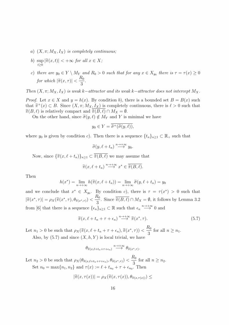
a) (X, π;MX , IX) is completely continuous;
b) supt≥0|π(x, t)| < +∞ for all x ∈ X;
c) there are y0 ∈ Y \MY and R0 > 0 such that for any x ∈ Xy0 there is τ = τ(x) ≥ 0
for which |π(x, τ)| < R0
3.
Then (X, π;MX , IX) is weak k−attractor and its weak k−attractor does not intercept MX .
Proof. Let x ∈ X and y = h(x). By condition b), there is a bounded set B = B(x) suchthat π+(x) ⊂ B. Since (X, π;MX , IX) is completely continuous, there is ` > 0 such thatπ(B, `) is relatively compact and π(B, `) ∩MX = ∅.
On the other hand, since σ(y, `) /∈MY and Y is minimal we have
y0 ∈ Y = σ+(σ(y, `)),
where y0 is given by condition c). Then there is a sequence tnn≥1 ⊂ R+ such that
σ(y, `+ tn)n→+∞−→ y0.
Now, since π(x, `+ tn)n≥1 ⊂ π(B, `) we may assume that
π(x, `+ tn)n→+∞−→ x∗ ∈ π(B, `).
Thenh(x∗) = lim
n→+∞h(π(x, `+ tn)) = lim
n→+∞σ(y, `+ tn) = y0
and we conclude that x∗ ∈ Xy0 . By condition c), there is τ = τ(x∗) > 0 such that
|π(x∗, τ)| = ρX(π(x∗, τ), θπ(x∗,τ)) <R0
3. Since π(B, `) ∩MX = ∅, it follows by Lemma 3.2
from [6] that there is a sequence εnn≥1 ⊂ R such that εnn→+∞−→ 0 and
π(x, `+ tn + τ + εn)n→+∞−→ π(x∗, τ). (5.7)
Let n1 > 0 be such that ρX(π(x, `+ tn + τ + εn), π(x∗, τ)) <R0
3for all n ≥ n1.
Also, by (5.7) and since (X, h, Y ) is local trivial, we have
θπ(x,`+tn+τ+εn)n→+∞−→ θπ(x∗,τ).
Let n2 > 0 be such that ρX(θπ(x,`+tn+τ+εn), θπ(x∗,τ)) <R0
3for all n ≥ n2.
Set n0 = maxn1, n2 and τ(x) := `+ tn0 + τ + εn0 . Then
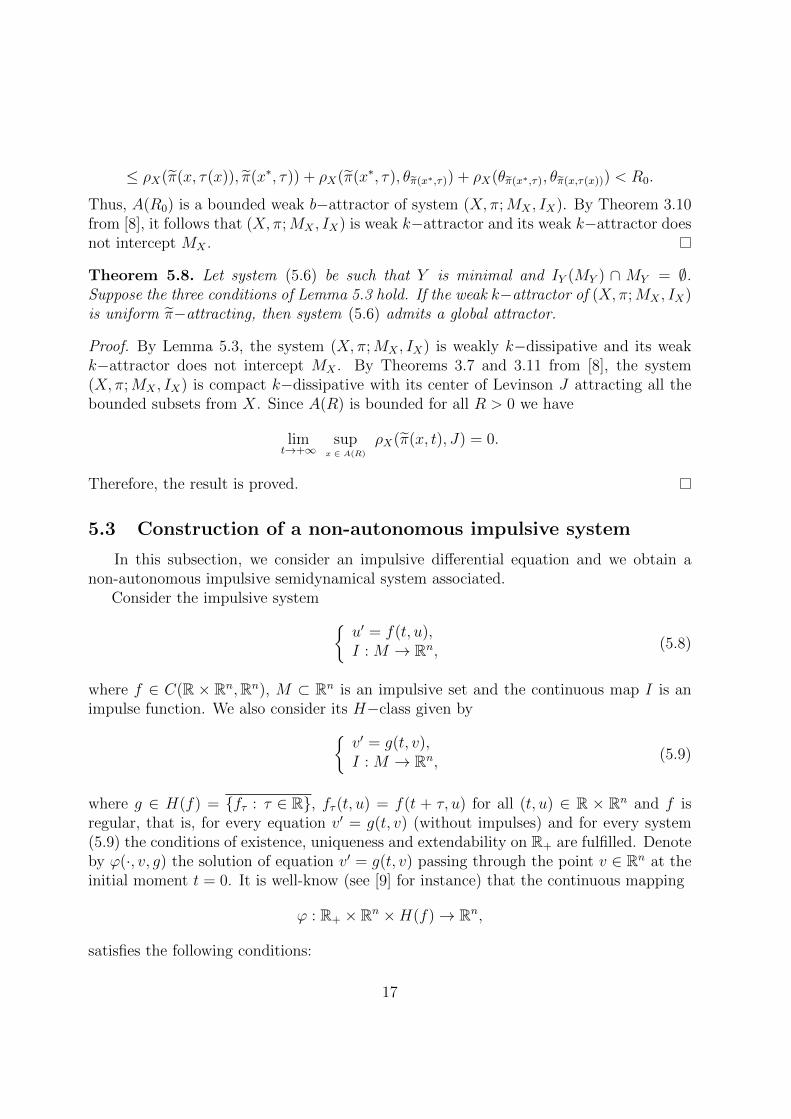
Thus, A(R0) is a bounded weak b−attractor of system (X, π;MX , IX). By Theorem 3.10from [8], it follows that (X, π;MX , IX) is weak k−attractor and its weak k−attractor doesnot intercept MX .
Theorem 5.8. Let system (5.6) be such that Y is minimal and IY (MY ) ∩ MY = ∅.Suppose the three conditions of Lemma 5.3 hold. If the weak k−attractor of (X, π;MX , IX)is uniform π−attracting, then system (5.6) admits a global attractor.
Proof. By Lemma 5.3, the system (X, π;MX , IX) is weakly k−dissipative and its weakk−attractor does not intercept MX . By Theorems 3.7 and 3.11 from [8], the system(X, π;MX , IX) is compact k−dissipative with its center of Levinson J attracting all thebounded subsets from X. Since A(R) is bounded for all R > 0 we have
limt→+∞
supx ∈ A(R)
ρX(π(x, t), J) = 0.
Therefore, the result is proved.
5.3 Construction of a non-autonomous impulsive system
In this subsection, we consider an impulsive differential equation and we obtain anon-autonomous impulsive semidynamical system associated.
Consider the impulsive system u′ = f(t, u),I : M → Rn, (5.8)
where f ∈ C(R × Rn,Rn), M ⊂ Rn is an impulsive set and the continuous map I is animpulse function. We also consider its H−class given by
v′ = g(t, v),I : M → Rn, (5.9)
where g ∈ H(f) = fτ : τ ∈ R, fτ (t, u) = f(t + τ, u) for all (t, u) ∈ R × Rn and f isregular, that is, for every equation v′ = g(t, v) (without impulses) and for every system(5.9) the conditions of existence, uniqueness and extendability on R+ are fulfilled. Denoteby ϕ(·, v, g) the solution of equation v′ = g(t, v) passing through the point v ∈ Rn at theinitial moment t = 0. It is well-know (see [9] for instance) that the continuous mapping
ϕ : R+ × Rn ×H(f)→ Rn,
satisfies the following conditions:
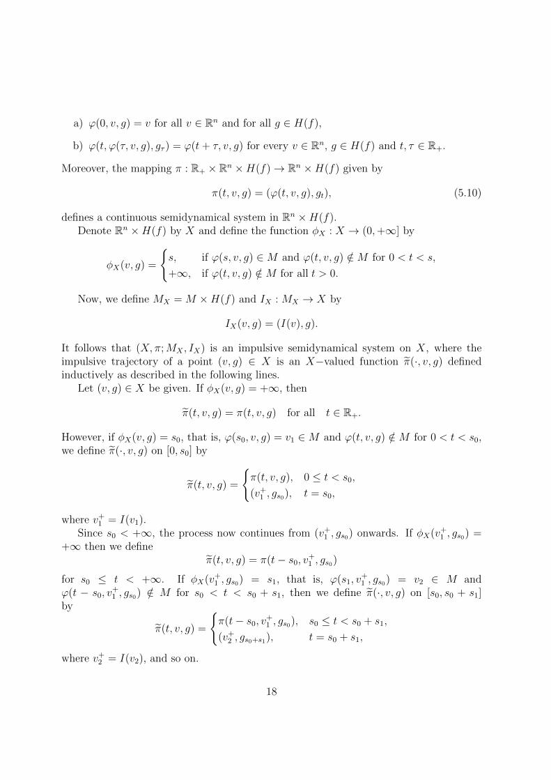
17
a) ϕ(0, v, g) = v for all v ∈ Rn and for all g ∈ H(f),
b) ϕ(t, ϕ(τ, v, g), gτ ) = ϕ(t+ τ, v, g) for every v ∈ Rn, g ∈ H(f) and t, τ ∈ R+.
Moreover, the mapping π : R+ × Rn ×H(f)→ Rn ×H(f) given by
π(t, v, g) = (ϕ(t, v, g), gt), (5.10)
defines a continuous semidynamical system in Rn ×H(f).Denote Rn ×H(f) by X and define the function φX : X → (0,+∞] by
φX(v, g) =
s, if ϕ(s, v, g) ∈M and ϕ(t, v, g) /∈M for 0 < t < s,
+∞, if ϕ(t, v, g) /∈M for all t > 0.
Now, we define MX = M ×H(f) and IX : MX → X by
IX(v, g) = (I(v), g).
It follows that (X, π;MX , IX) is an impulsive semidynamical system on X, where theimpulsive trajectory of a point (v, g) ∈ X is an X−valued function π(·, v, g) definedinductively as described in the following lines.
Let (v, g) ∈ X be given. If φX(v, g) = +∞, then
π(t, v, g) = π(t, v, g) for all t ∈ R+.
However, if φX(v, g) = s0, that is, ϕ(s0, v, g) = v1 ∈M and ϕ(t, v, g) /∈M for 0 < t < s0,we define π(·, v, g) on [0, s0] by
π(t, v, g) =
π(t, v, g), 0 ≤ t < s0,
(v+1 , gs0), t = s0,
where v+1 = I(v1).
Since s0 < +∞, the process now continues from (v+1 , gs0) onwards. If φX(v+
1 , gs0) =+∞ then we define
π(t, v, g) = π(t− s0, v+1 , gs0)
for s0 ≤ t < +∞. If φX(v+1 , gs0) = s1, that is, ϕ(s1, v
+1 , gs0) = v2 ∈ M and
ϕ(t − s0, v+1 , gs0) /∈ M for s0 < t < s0 + s1, then we define π(·, v, g) on [s0, s0 + s1]
by
π(t, v, g) =
π(t− s0, v
+1 , gs0), s0 ≤ t < s0 + s1,
(v+2 , gs0+s1), t = s0 + s1,
where v+2 = I(v2), and so on.
18
Let MY ⊂ H(f) be an impulsive set and IY : MY → H(f) be the identity IY (g) = g.Note in this case that the impulsive system (H(f), σ;MY , IY ) is a continuous semidynam-ical system. Then
〈(X, π;MX , IX), (H(f), σ;MY , IY ), h〉,where h is the projection in the second coordinate, is a non-autonomous impulsive semi-dynamical system associated to the system (5.8).
References
[1] S. M. Afonso, E. M. Bonotto, M. Federson and S. Schwabik, Discontinuous local semi-flows for Kurzweil equations leading to LaSalle’s invariance principle for differentialsystems with impulses at variable times, J. Diff. Equations, 250 (2011), 2969-3001.
[2] R. Ambrosino, F. Calabrese, C. Cosentino and G. De Tommasi, Sufficient condi-tions for finite-time stability of impulsive dynamical systems. IEEE Trans. Automat.Control, 54 (2009), 861-865.
[3] L. Barreira and C. Valls, Lyapunov regularity of impulsive differential equations, J.Diff. Equations, 249 (7), (2010), 1596-1619.
[4] B. Bouchard, Ngoc-Minh Dang and Charles-Albert Lehalle, Optimal Control of Trad-ing Algorithms: A General Impulse Control Approach, SIAM J. Finan. Math., 2(2011), 404-438.
[5] E. M. Bonotto and M. Federson, Topological conjugation and asymptotic stabilityin impulsive semidynamical systems. J. Math. Anal. Appl., 326 (2007), 869-881.
[6] E. M. Bonotto, Flows of characteristic 0+ in impulsive semidynamical systems, J.Math. Anal. Appl., 332 (1), (2007), 81-96.
[7] E. M. Bonotto and D. P. Demuner, Autonomous dissipative semidynamical systemswith impulses. Topological Methods in Nonlinear Analysis., v.41 (1), (2013), 1-38.
[8] E. M. Bonotto and D. P. Demuner, Attractors of impulsive dissipative semidynamicalsystems. Bulletin des Sciences Mathematiques, 137 (2013), 617-642.
[9] D. N. Cheban, Global attractors of non-autonomous dissipative dynamical systems,Interdiscip. Math. Sci., vol. 1, World Scientific Publishing, Hackensack, NJ, 2004.
[10] K. Ciesielski, On semicontinuity in impulsive dynamical systems, Bull. Polish Acad.Sci. Math., 52 (2004), 71-80.
[11] K. Ciesielski, On stability in impulsive dynamical systems, Bull. Polish Acad. Sci.Math., 52 (2004), 81-91.
19
[12] M. H. A. Davis, X. Guo and Guoliang Wu, Impulse Control of MultidimensionalJump Diffusions, SIAM J. Control Optim., 48 (2010), 5276-5293.
[14] C. Ding, Limit sets in impulsive semidynamical systems, Topol. Methods in NonlinearAnal., 43 (2014), 97-115.
[15] W. M. Haddad and Q. Hui, Energy dissipating hybrid control for impulsive dynamicalsystems. Nonlinear Anal., 69 (2008), 3232-3248.
[16] D. Husemoller, Fibre bundles. Springer-Verlag, Berlin-Heidelberg-New York, 1994.
[17] S. K. Kaul, On impulsive semidynamical systems, J. Math. Anal. Appl., 150 (1),(1990), 120-128.
[18] S. K. Kaul, On impulsive semidynamical systems II - recursive properties, NonlinearAnalysis: Theory, Methods & Applications, 7-8 (1991), 635-645.
[19] S. K. Kaul, Stability and asymptotic stability in impulsive semidynamical systems,J. Applied Math. and Stochastic Analysis, 7(4) (1994), 509-523.
[20] V. Lakshmikantham, D.D. Bainov, P.S. Simeonov, Theory of Impulsive DifferentialEquations, World Scientific, Singapore, 1989.
[21] Yang Jin and Zhao Min, Complex behavior in a fish algae consumption model withimpulsive control strategy. Discrete Dyn. Nat. Soc. Art., ID 163541, (2011), 17 pp.
[22] H. Ye, A. N. Michel and L. Hou, Stability analysis of systems with impulse effects,IEEE Transactions on Automatic Control, 43 (12), (1998), 1719-1723.
[23] Zhao L., Chen L. and Zhang Q., The geometrical analysis of a predator-prey modelwith two state impulses, Mathematical Biosciences, 238 (2), (2012), 55-64.
Everaldo de Mello Bonotto
Instituto de Ciencias Matematicas e de Computacao,Universidade de Sao Paulo, Caixa Postal 668, Sao Carlos SP, Brazil.