Universidade de São Paulo Escola Superior de Agricultura “Luiz de Queiroz” Mobile terrestrial laser scanner for site-specific management in orange crop André Freitas Colaço Thesis presented to obtain the degree of Doctor in Science. Area: Agricultural Systems Engineering Piracicaba 2016
Transcript
Universidade de São Paulo Escola Superior de Agricultura “Luiz de Queiroz”
Mobile terrestrial laser scanner for site-specific management in orange crop
André Freitas Colaço
Thesis presented to obtain the degree of Doctor in Science. Area: Agricultural Systems Engineering
Piracicaba 2016
André Freitas Colaço Agronomist
Mobile terrestrial laser scanner for site-specific management in orange crop
Advisor: Prof. Dr. JOSÉ PAULO MOLIN Co-advisor: Prof. Dr. ALEXANDRE ESCOLÀ AGUSTÍ
Thesis presented to obtain the degree of Doctor in Science. Area: Agricultural Systems Engineering
Piracicaba 2016
2
Dados Internacionais de Catalogação na Publicação
DIVISÃO DE BIBLIOTECA – DIBD/ESALQ/USP
Colaço, André Freitas
Mobile terrestrial laser scanner for site-specific management in orange crop / André Freitras Colaço. - - Piracicaba, 2016.
87 p.
Tese (Doutorado) - - USP / Escola Superior de Agricultura “Luiz de Queiroz”.
1. Sensor LiDAR 2. Geometria de copa 3. Tecnologia de taxa variada 4. Agricultura de precisão. I. Título
3
ACKNOWLEDGEMENTS
My sincere thankfulness,
To the University of São Paulo and the ‘Luiz de Queiroz’ College of Agriculture, for technical, social and scientific
education.
To Fapesp and Capes for providing financial means to my formation.
To Jacto and Citrosuco companies, for providing the equipment and experimental fields.
To Prof. José Paulo Molin, for guidance and opportunities throughout my academic life.
To Prof. Alexandre Escolà Agustí, the codirector of this project, for giving good ideas to this work. Also, for kindly
hosting me in Spain.
To all my friends in Lleida, the members of the Research Group in AgroICT and Precision Agriculture, especially to
Prof. Joan Ramón Rosell Polo for providing me a good experience at the University of Lleida.
To my friends and colleges from the Biosystems Engineering Department, Adriano A. Anselmi, Felippe H. S. Karp,
Gustavo Portz, Jeovano G. A. Lima, João Paulo S. Veiga, Leonardo F. Maldaner, Lucas R. Amaral, Marcos N.
Ferraz, Mark Spekken, Mateus T. Eitelwein, Natanael S. Vilanova, Nelson C. Franco Jr., Rodrigo G. Trevisan,
Tatiana F. Canata and Thiago L. Romanelli.
To my friends for life, Camila, Diego, Erik, Heitor, Leonardo, Mônica and Viviane.
To my family in blood and in law, for the incentive.
To my lovely Larissa, who makes me happy every day with her love and kind companionship.
To my parents, brother and sister, Ailton, Lucy, Rafael and Raquel, my role models to whom I own everything.
4
“The theory of emptiness…is the deep recognition that there is a fundamental disparity between the
way we perceive the world, including our own existence in it, and the way things actually are.”
Dalai Lama XIV, The Universe in a Single Atom: The Convergence of Science and Spirituality
LIST OF FIGURES ....................................................................................................................................................... 8
LIST OF TABLES ....................................................................................................................................................... 10
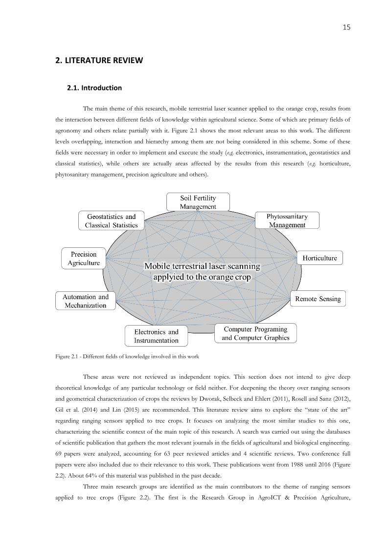
2. LITERATURE REVIEW ........................................................................................................................................... 15
2.1. Introduction .......................................................................................................................................................15 2.2. Ranging sensors applied to tree crops .............................................................................................................16 References ................................................................................................................................................................26
3. ORANGE CROP GEOMETRY AND 3D MODELING USING A MOBILE TERRESTRIAL LASER SCANNER ...................... 31
3.3.1. Description of the data acquisition and processing ................................................................................34 3.3.2. Demonstrating and testing the proposed methods ................................................................................41
3.4. Results and Discussion ......................................................................................................................................45 3.4.1. Point cloud generation - laboratory testing .............................................................................................45 3.4.2. Field scanning and 3D modeling ...............................................................................................................46 3.4.3. Mapping of canopy volume and height ...................................................................................................52
4.3.1. Field characteristics ...................................................................................................................................61 4.3.2. LiDAR data acquisition and processing ....................................................................................................62 4.3.3. Variability of canopy geometry and potential benefit of sensor-based variable rate applications ......62 4.3.4. Spatial variability of canopy geometry .....................................................................................................63 4.3.5. Relationship between tree geometry, soil attributes and historical yield .............................................64
4.4. Results and Discussion ......................................................................................................................................66 4.4.1. Variability of canopy geometry and potential benefit of sensor-based variable rate applications ......66 4.4.2. Spatial variability of canopy geometry .....................................................................................................72 4.4.3. Relationship between tree geometry and soil attributes and historical yield .......................................76
5. SUMMARY AND FINAL REMARKS ........................................................................................................................ 87
6
RESUMO
Sensor a laser na gestão localizada de pomares de laranja
Sensores baseados em tecnologia LiDAR (Light Detection and Ranging) têm o potencial de fornecer modelos tridimensionais de árvores, provendo informações como o volume e altura de copa. Essas informações podem ser utilizadas em diagnósticos e recomendações localizadas de fertilizantes e defensivos agrícolas. Este estudo teve como objetivo investigar o uso de sensores LiDAR na cultura da laranja, uma das principais culturas de porte arbóreo no Brasil. Diversas pesquisas têm desenvolvido sistemas LiDAR para culturas arbóreas. Porém, normalmente tais sistemas são empregados em plantas individuais ou em pequenas áreas. Dessa forma, diversos aspectos da aquisição e processamento de dados ainda devem ser desenvolvidos para viabilizar a aplicação em larga escala. O primeiro estudo deste documento (Capítulo 3) focou no desenvolvimento de um sistema LiDAR (Mobile Terrestrial Laser Scanner - MTLS) e nova metodologia de processamento de dados para obtenção de informações acerca da geometria das copas em pomares comerciais de laranja. Um sensor a laser e um receptor RTK-GNSS (Real Time Kinematics - Global Navigation Satellite System) foram instalados em um veículo para leituras em campo. O processamento de dados foi baseado na geração de uma nuvem de pontos, seguida dos passos de filtragem, classificação e reconstrução da superfície das copas. Um pomar comercial de laranja de 25 ha foi utilizado para a validação. O sistema de aquisição e processamento de dados foi capaz de produzir uma nuvem de pontos representativa do pomar, fornecendo informação sobre geometria das plantas em alta resolução. A escolha sobre o tipo de classificação da nuvem de pontos (em plantas individuais ou em seções transversais das fileiras) e sobre o algoritmo de reconstrução de superfície, foi discutida nesse estudo. O segundo estudo (Capítulo 4) buscou caracterizar a variabilidade espacial da geometria de copa em pomares comerciais. Entender tal variabilidade permite avaliar se a aplicação em taxas variáveis de insumos baseada em sensores LiDAR (aplicar quantias de insumos proporcionais ao tamanho das copas) é uma estratégia adequada para otimizar o uso de insumos. Cinco pomares comerciais foram avaliados com o sistema MTLS. De acordo com a variabilidade encontrada, a economia de insumos pelo uso da taxa variável foi estimada em aproximadamente 40%. O segundo objetivo desse estudo foi avaliar a relação entre a geometria de copa e diversos outros parâmetros dos pomares. Os mapas de volume e altura de copa foram comparados aos mapas de produtividade, elevação, condutividade elétrica do solo, matéria orgânica e textura do solo. As correlações entre geometria de copa e produtividade ou fatores de solo variaram de fraca até forte, dependendo do pomar. Quando os pomares foram divididos entre três classes com diferentes tamanhos de copas, o desempenho em produtividade e as características do solo foram distintas entre as três zonas, indicando que parâmetros de geometria de copa são variáveis úteis para a delimitação de unidades de gestão diferenciada em um pomar. Os resultados gerais desta pesquisa mostraram o potencial de sistemas MTLS para pomares de laranja, indicando como a geometria de copa pode ser utilizada na gestão localizada de pomares de laranja.
Palavras-chave: Sensor LiDAR; Geometria de copa; Tecnologia de taxa variada; Agricultura de precisão
7
ABSTRACT
Mobile terrestrial laser scanner for site-specific management in orange crop
Sensors based on LiDAR (Light Detection and Ranging) technology have the potential to provide accurate 3D models of the trees retrieving information such as canopy volume and height. This information can be used for diagnostics and prescriptions of fertilizers and plant protection products on a site-specific basis. This research aimed to investigate the use of LiDAR sensors in orange crops. Orange is one of the most important tree crop in Brazil. So far, research have developed and tested LiDAR based systems for several tree crops. However, usually individual trees or small field plots have been used. Therefore, several aspects related to data acquisition and processing must still be developed for large-scale application. The first study reported in this document (Chapter 3) aimed to develop and test a mobile terrestrial laser scanner (MTLS) and new data processing methods in order to obtain 3D models of large commercial orange groves and spatial information about canopy geometry. A 2D laser sensor and a RTK-GNSS receiver (Real Time Kinematics - Global Navigation Satellite System) were mounted on a vehicle. The data processing was based on generating a georeferenced point cloud, followed by the filtering, classification and surface reconstruction steps. A 25 ha commercial orange grove was used for field validation. The developed data acquisition and processing system was able to produce a reliable point cloud of the grove, providing high resolution canopy volume and height information. The choice of the type of point cloud classification (by individual trees or by transversal sections of the row) and the surface reconstruction algorithm is discussed in this study. The second study (Chapter 4) aimed to characterize the spatial variability of canopy geometry in commercial orange groves. Understanding such variability allows sensor-based variable rate application of inputs (i.e, applying proportional rates of inputs based on the variability of canopy size) to be considered as a suitable strategy to optimize the use of fertilizers and plant protection products. Five commercial orange groves were scanned with the developed MTLS system. According to the variability of canopy volume found in those groves, the input savings as a result of implementing sensor-based variable rate technologies were estimated in about 40%. The second goal of this study was to understand the relationship between canopy geometry and several other relevant attributes of the groves. The canopy volume and height maps of three groves were analyzed against historical yield maps, elevation, soil electrical conductivity, organic matter and clay content maps. The correlations found between canopy geometry and yield or soil maps varied from poor to strong correlations, depending on the grove. When classifying the groves into three classes according to canopy size, the yield performance and soil features inside each class was found to be significantly different, indicating that canopy geometry is a suitable variable to guide management zones delineation in one grove. Overall results from this research show the potential of MTLS systems and subsequent data analysis in orange crops indicating how canopy geometry information can be used in site-specific management practices.
Figure 2.1 Different fields of knowledge involved in this work ............................................................................................. 15
Figure 2.2: Sources of the reviewed papers and publication rate of different research groups ........................................ 16
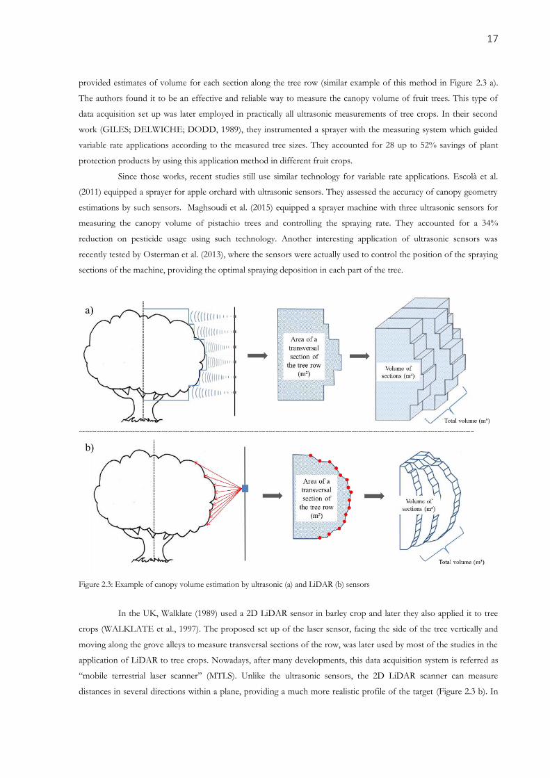
Figure 2.3: Example of canopy volume estimation by ultrasonic (a) and LiDAR (b) sensors .......................................... 17
Figure 2.4: Transformed LiDAR data into a distance image; adapted from Tumbo et al. (2002) and Wei and Salyani
Figure 2.6: Prototype sprayer with ultrasonic measuring system (a) and scheme of ultrasonic estimation of canopy
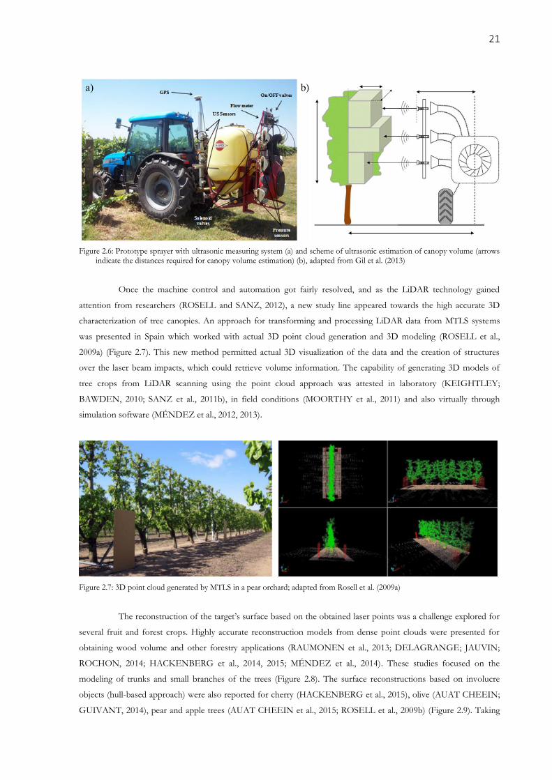
volume (arrows indicate the distances required for canopy volume estimation) (b), adapted from Gil et al. (2013) ... 21
Figure 2.7: 3D point cloud generated by MTLS in a pear orchard; adapted from Rosell et al. (2009a) .......................... 21
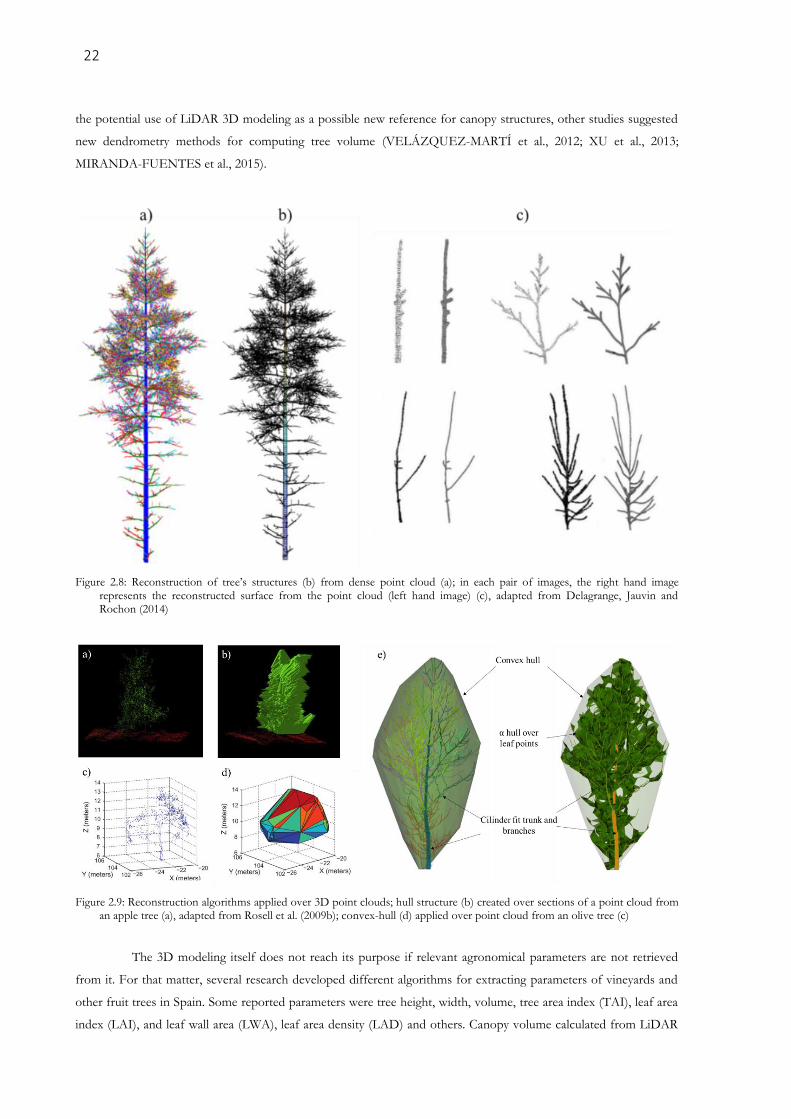
Figure 2.8: Reconstruction of tree’s structures (b) from dense point cloud (a); in each pair of images, the right hand
image represents the reconstructed surface from the point cloud (left hand image) (c), adapted from Delagrange,
Jauvin and Rochon (2014) ............................................................................................................................................................. 22
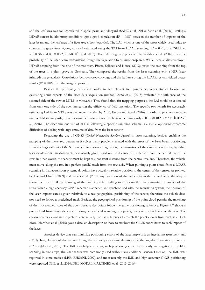
Figure 2.9: Reconstruction algorithms applied over 3D point clouds. Hull structure (b) created over sections of a
point cloud from an apple tree (a), adapted from Rosell et al. (2009b). Convex-hull (d) applied over point cloud from
an olive tree (c) ................................................................................................................................................................................. 22
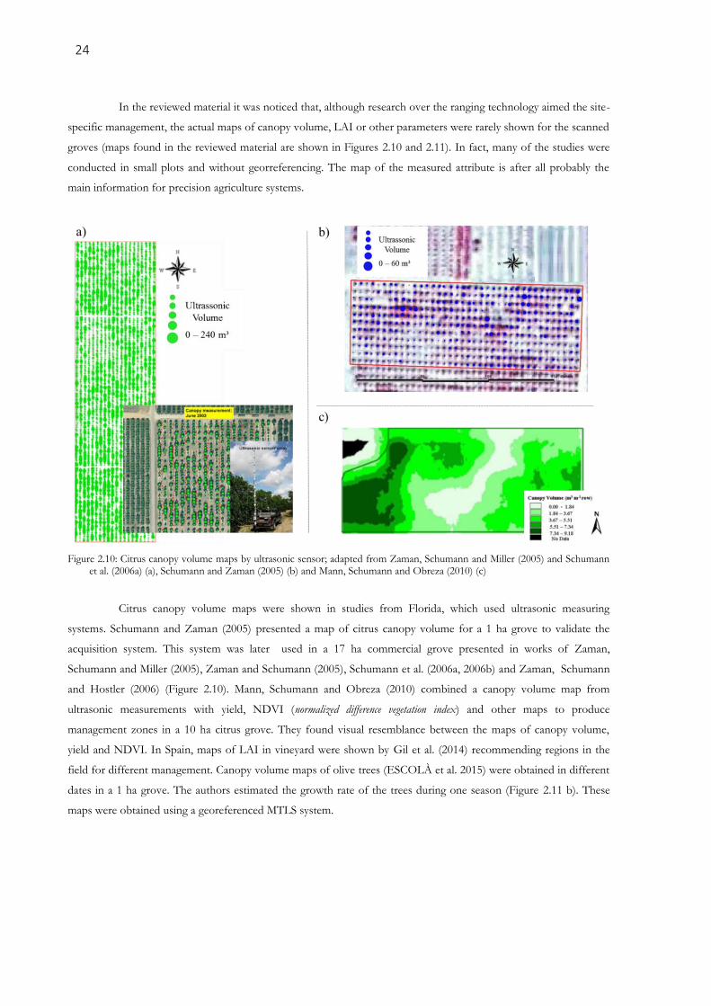
Figure 2.10: Citrus canopy volume maps by ultrasonic sensor; adapted from Zaman, Schumann and Miller (2005)
and Schumann et al. (2006a) (a), Schumann and Zaman (2005) (b) and Mann, Schumann and Obreza (2010) (c) ..... 24
Figure 2.11: Maps of LAI in vineyard (a) adapted from Gil et al. (2014) and canopy volume in an olive grove (b)
adapted from Escolà et al. (2015) ................................................................................................................................................. 25
Figure 3.1: LiDAR sensor Sick, LMS 200 (a) and angular range on 2D scanning plane (b) (adapted from SICK AG.,
Figure 3.2: LiDAR sensor and RTK-GNSS receiver mounted on an all-terrain vehicle (a); diagram of LiDAR sensor
displacement along the alleys (b) .................................................................................................................................................. 35
Figure 3.3: Output file from the data acquisition software containing information of the RTK-GNSS receiver and the
measured LiDAR distances in mm .............................................................................................................................................. 36
Figure 3.4: RTK base station (a); track of the vehicle for scanning both sides of the tree rows (b) ................................ 37
Figure 3.5: dx and dy deviations based on the angle α and dxy (a); dxy based on distance d and angle β (b) ................ 38
Figure 3.6: Original point cloud from one tree row (a); point cloud after the filtering process (b) ................................. 39
Figure 3.7: The x and y coordinates of a point cloud from orange trees (a); and clustering classification into groups
each representing one individual tree (b) .................................................................................................................................... 40
Figure 3.8: Top view of a point cloud; segmentation of the tree row (a); classified points in transversal sections (b). 41
Figure 3.9: 25 ha commercial orange grove scanned with the laser sensor .......................................................................... 42
Figure 3.10: Merging of adjacent sections of the row into segments equivalent to the tree spacing ............................... 44
Figure 3.11: Point clouds from objects scanned by a mobile terrestrial laser scanner mounted on an all-terrain
vehicle; cylinder (a), body of cone (b), square (c), triangle (d) and circle (e)......................................................................... 45
Figure 3.12: Point cloud derived from the developed terrestrial laser scanning system in a 25 ha commercial orange
grove .................................................................................................................................................................................................. 47
9
Figure 3.13: Convex-hull and alpha-shape algorithms to model orange trees by two approaches: clusters (individual
tree) and transversal sections of the row (0.26 m wide) ........................................................................................................... 48
Figure 3.14: Detail of the convex-hull and alpha-shape modeled over a single 0.26 m wide transversal section of a
tree row ............................................................................................................................................................................................. 49
Figure 3.15: Top view of the convex-hull modeling over transversal sections of an orange tree row ............................ 49
Figure 3.16: 3D canopy structure of a single tree modeled by different algorithms ........................................................... 50
Figure 3.17: Canopy volume computation by different algorithms for individual trees and by dividing each tree into
three, five, seven and ten transversal sections ............................................................................................................................ 51
Figure 3.18: Canopy volume of 25 individual trees computed by different methods ......................................................... 51
Figure 3.19: Shapefile resulted from data processing according to the method based on segmenting the row into
Figure 3.20: Shapefile resulted from the data processing method based on cluster analysis and single-tree
computation of canopy volume .................................................................................................................................................... 53
Figure 3.21: Canopy volume maps generated by two data processing methods: Alpha-shape modeled over individual
trees (Method 1); Convex-hull modeled over sections of the row (Method 2) ................................................................... 54
Figure 3.22: Canopy height maps generated by two data processing methods: Alpha-shape modeled over individual
trees (Method 1); Convex-hull modeled over sections of the row (Method 2) ................................................................... 55
Figure 3.23: Fuzzy similarity maps resulted from the comparison between maps of canopy volume (a) and canopy
height (b) generated by two different methods (cluster segmentation using alpha-shape reconstruction and
transversal section segmentation using convex-hull reconstruction) ..................................................................................... 55
Figure 4.1: Overview of the orange groves 1 to 5 used in the study ..................................................................................... 62
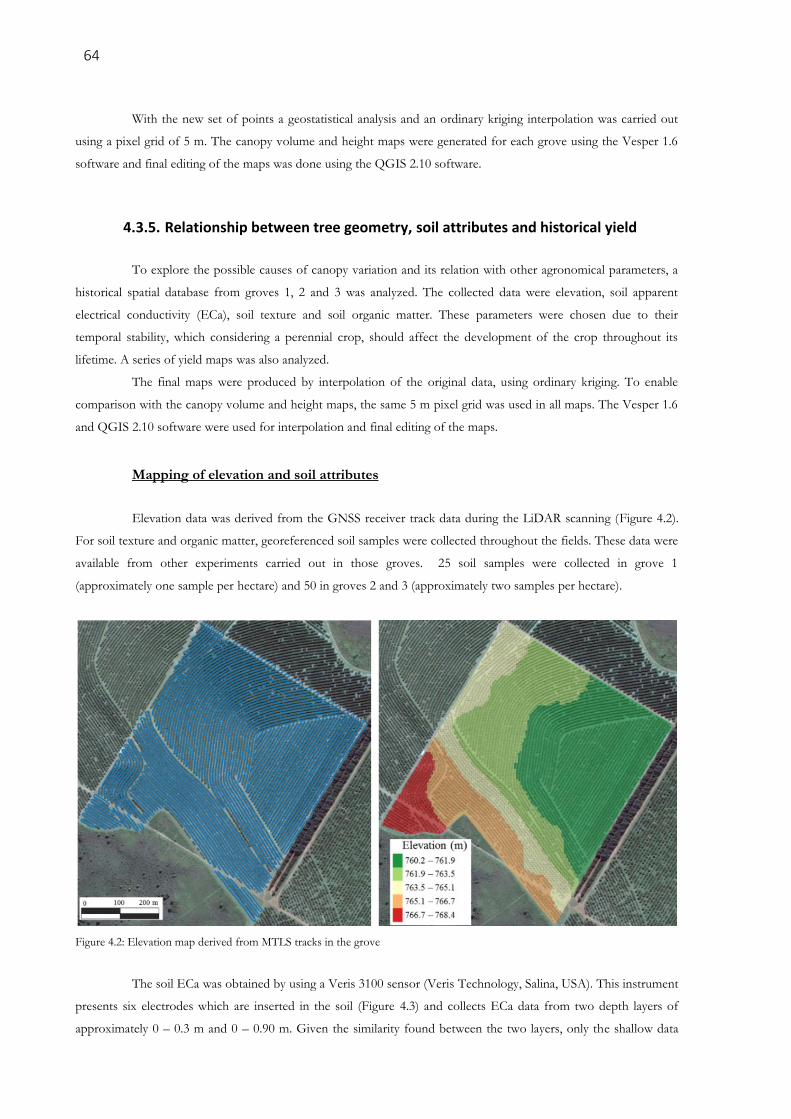
Figure 4.2: Elevation map derived from MTLS tracks in the grove ...................................................................................... 64
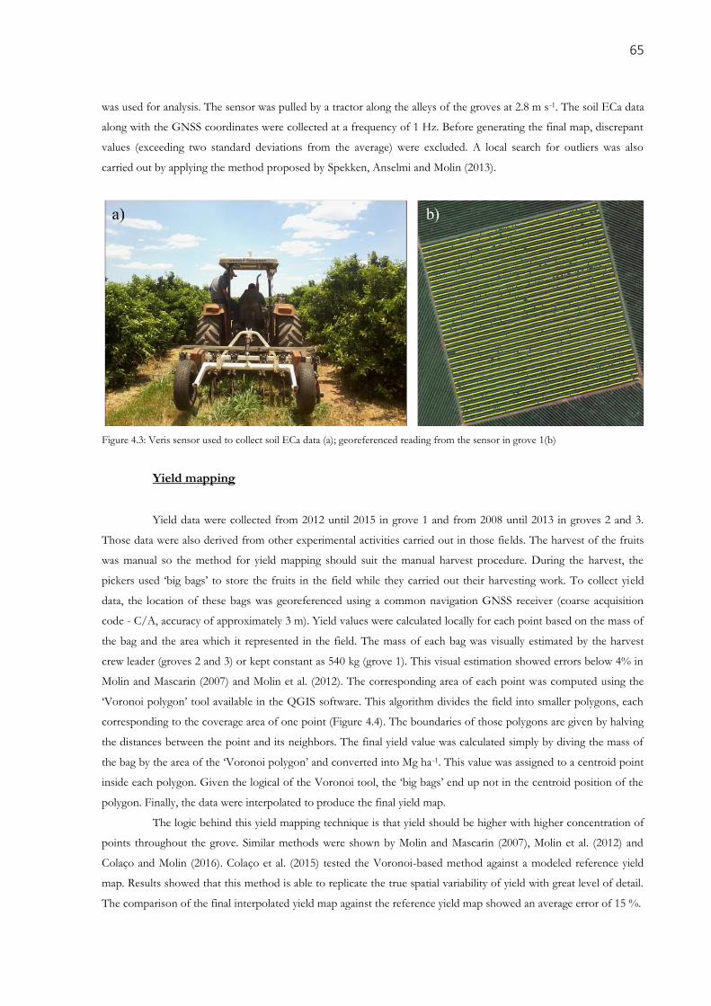
Figure 4.3: Veris sensor used to collect soil ECa data (a); georeferenced reading from the sensor in grove 1(b) ......... 65
Figure 4.4: Georeferenced big bags and computed ‘Voronoi’ polygon (a); calculation of local yield in each point ..... 66
Figure 4.5: Canopy volume (left) and height (right) histograms for 0.25 m sections along the crop rows ..................... 69
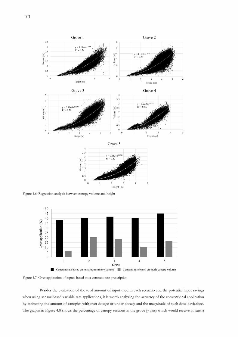
Figure 4.6: Regression analysis between canopy volume and height ..................................................................................... 70
Figure 4.7: Over application of inputs based on a constant rate prescription ..................................................................... 70
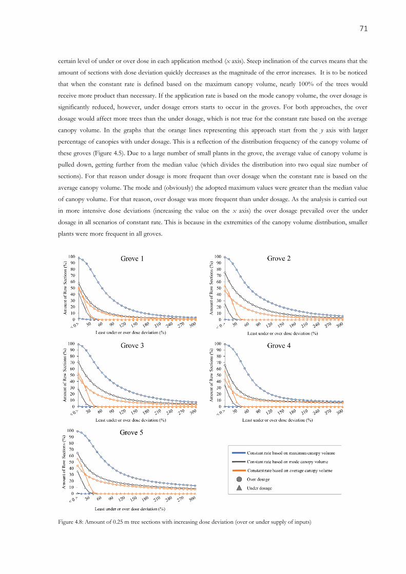
Figure 4.8: Amount of 0.25 m tree sections with increasing dose deviation (over or under supply of inputs) ............. 71
Figure 4.9: Variogram of canopy volume and canopy height in different groves ............................................................... 72
Figure 4.10: Canopy volume and height maps of in groves 1, 2 and 3.................................................................................. 74
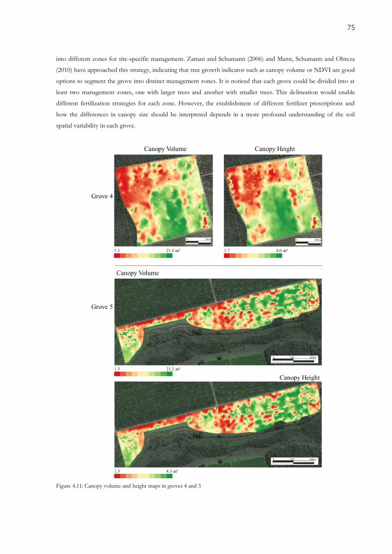
Figure 4.11: Canopy volume and height maps in groves 4 and 5 ........................................................................................... 75
Figure 4.12: Maps of soil attributes and historical yield in grove 1 ........................................................................................ 77
Figure 4.13: Maps of soil attributes and historical yield in grove 2 ........................................................................................ 78
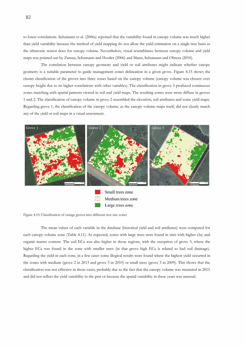
Figure 4.14: Maps of soil attributes and historical yield in grove 3 ........................................................................................ 80
Figure 4.15: Classification of orange groves into different tree size zones ........................................................................... 82
10
LIST OF TABLES
Table 3.1: Configuration used for the LiDAR sensor............................................................................................................... 42
Table 3.2: Object dimensions measured manually and by a mobile terrestrial laser scanner mounted on an all-terrain
vehicle and on a platform running over a rail ............................................................................................................................ 46
Table 3.3: Mean canopy volume of 25 individual trees by different methods and by dividing the trees into different
number of sections .......................................................................................................................................................................... 50
Table 3.4: Descriptive statistics of canopy volume and height for the two methods ......................................................... 54
Table 4.1: General characteristics of the orange groves used in this study ........................................................................... 61
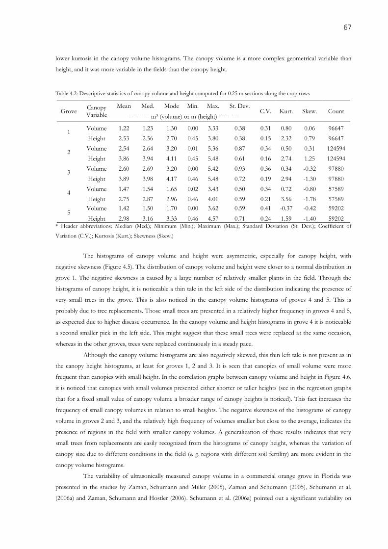
Table 4.2: Descriptive statistics of canopy volume and height computed for 0.25 m sections along the crop rows .... 67
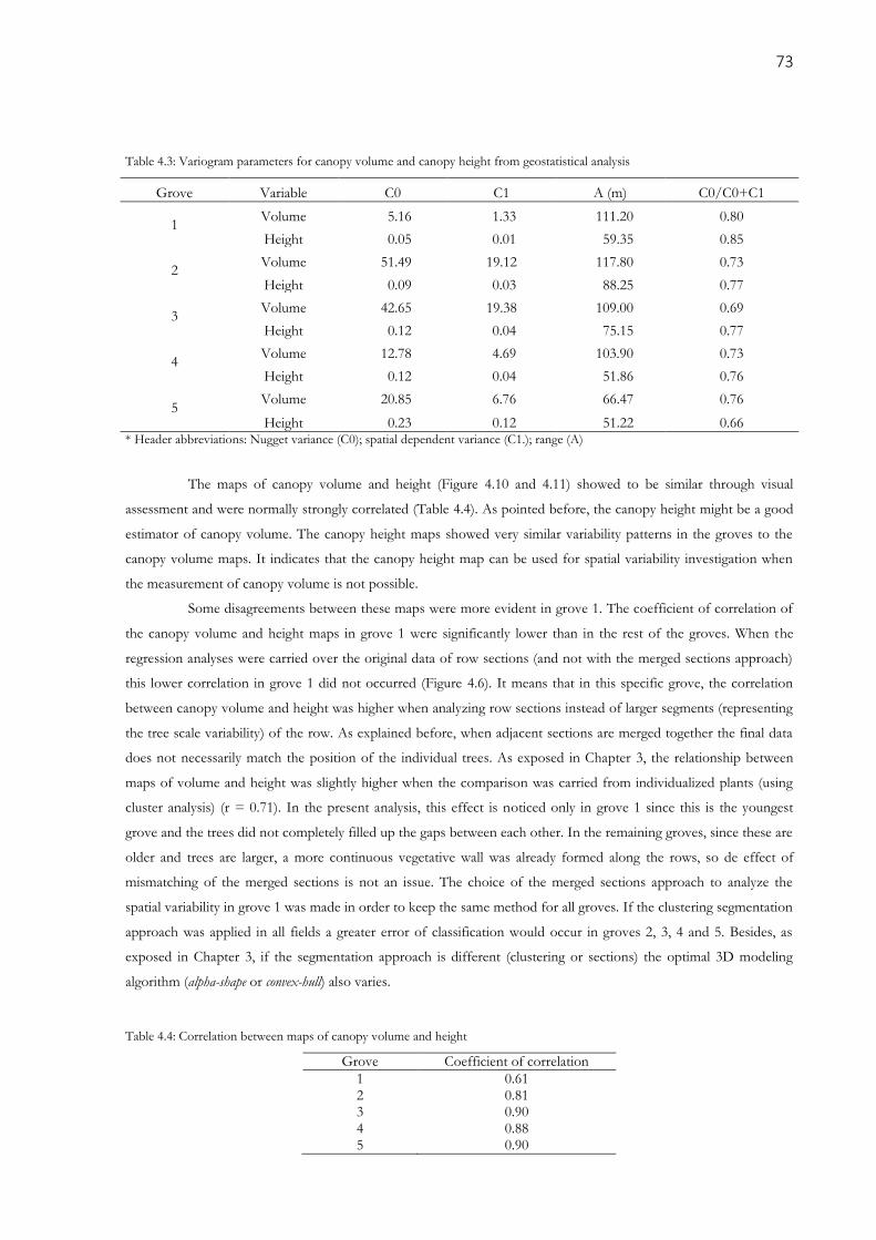
Table 4.3: Variogram parameters for canopy volume and canopy height from geostatistical analysis ............................ 73
Table 4.4: Correlation between maps of canopy volume and height ..................................................................................... 73
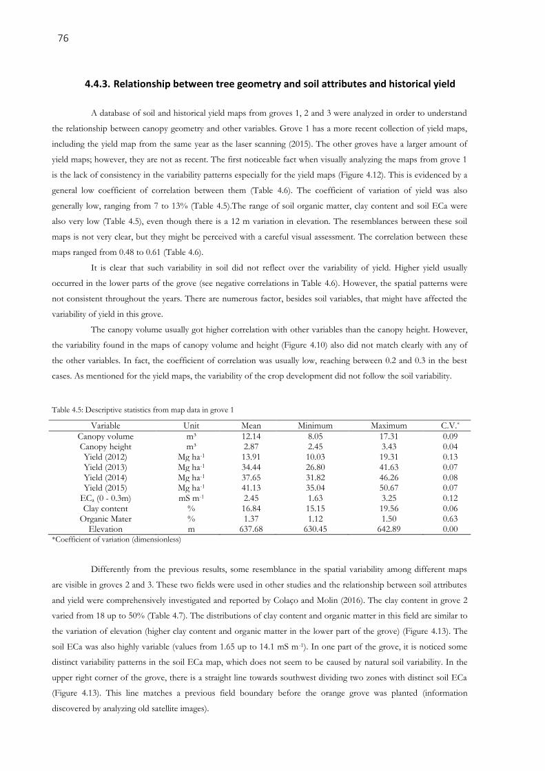
Table 4.5: Descriptive statistics from map data in grove 1 ...................................................................................................... 76
Table 4.6: Correlation matrix between different maps in grove 1 .......................................................................................... 77
Table 4.7: Descriptive statistics from map data in grove 2 ...................................................................................................... 78
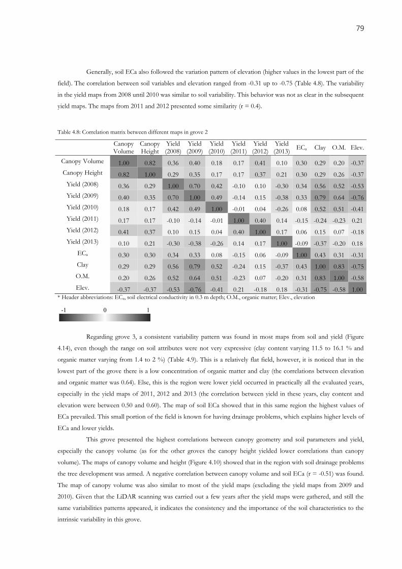
Table 4.8: Correlation matrix between different maps in grove 2 .......................................................................................... 79
Table 4.9: Descriptive statistics from map data in grove 3 ...................................................................................................... 80
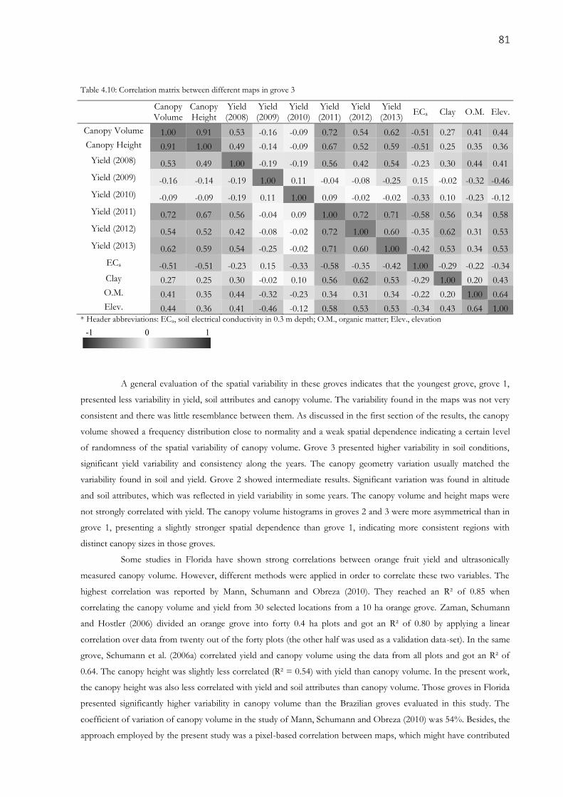
Table 4.10: Correlation matrix between different maps in grove 3 ........................................................................................ 81
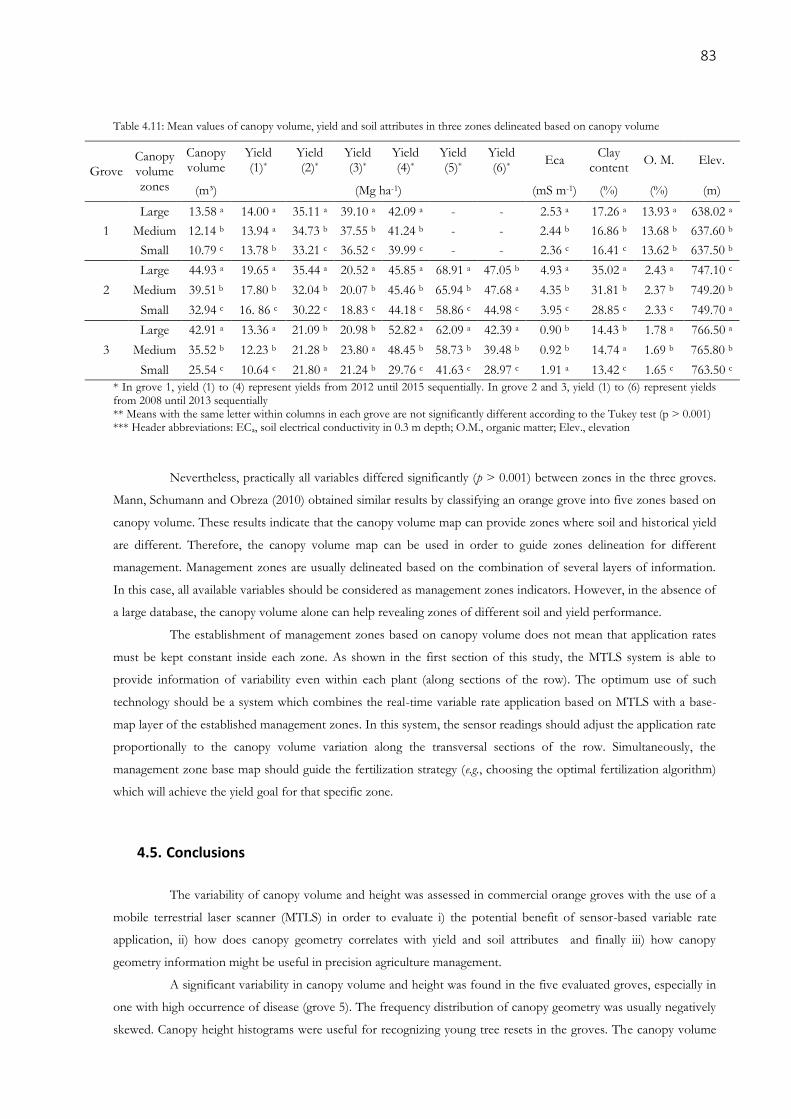
Table 4.11: Mean values of canopy volume, yield and soil attributes in three zones delineated based on canopy
R. Innovative LIDAR 3D Dynamic Measurement System to estimate fruit-tree leaf area. Sensors, New York, v.
11, n. 6, p. 5769–91, 2011a.
SANZ, R.; LLORENS, J.; ROSELL, J. R.; GREGORIO, E.; PALACÍN, J. Characterisation of the LMS200 laser
beam under the influence of blockage surfaces. Influence on 3D scanning of tree orchards. Sensors, New York,
v. 11, n. 3, p. 2751–72, 2011b.
SANZ, R.; ROSELL, J. R.; LLORENS, J.; GIL, E.; PLANAS, S. Relationship between tree row LIDAR-volume and
leaf area density for fruit orchards and vineyards obtained with a LIDAR 3D Dynamic Measurement System.
Agricultural and Forest Meteorology, Amsterdam, v. 171-172, p. 153–162. 2013.
SCHUMANN, A. W.; HOSTLER, K. H.; BUCHANON, S.; ZAMAN, Q. U. Relating citrus canopy size and yield to
precision fertilization. Proceedings of Florida State Horticultural Society, Tallahassee, v. 119, p. 148–154,
2006a.
SCHUMANN, A. W.; MILLER, W. M.; ZAMAN, Q. U.; HOSTLER, K. H.; BUCHANON, S.; CUGATI, S. A.
Variable rate granular fertilization of citrus groves: Spreader performance with single-tree prescription zones.
Applied Engineering in Agriculture, St. Joseph, v. 22, n. 1, p. 19–24, 2006b.
SCHUMANN, A. W.; ZAMAN, Q. U. Software development for real-time ultrasonic mapping of tree canopy size.
Computers and Electronics in Agriculture, Amsterdam, v. 47, n. 1, p. 25–40, 2005.
SOLANELLES, F.; ESCOLÀ, A.; PLANAS, S.; ROSELL, J. R.; CAMP, F.; GRÀCIA, F. An electronic control
system for pesticide application proportional to the canopy width of tree crops. Biosystems Engineering,
London, v. 95, n. 4, p. 473–481, 2006.
TUMBO, S. D.; SALYANI, M.; WHITNEY, J. D.; WHEATON, T. A.; MILLER, W. M. Investigation of laser and
ultrasonic ranging sensors for measurements of citrus canopy volume. Applied Engineering in Agriculture,
St. Joseph, v. 18, n. 3, p. 367–372, 2002.
VELÁZQUEZ-MARTÍ, B.; ESTORNELL, J.; LÓPEZ-CORTÉS, I.; MARTÍ-GAVILÁ, J. Calculation of biomass
volume of citrus trees from an adapted dendrometry. Biosystems Engineering, London, v. 112, n. 4, p. 285–
292, 2012.
WALKLATE, P. J. A laser scanning instrument for measuring crop geometry. Agricultural and Forest
Meteorology, Amsterdam, v. 46, p. 275–284, 1989.
WALKLATE, P. J.; CROSS, J. V. An examination of Leaf-Wall-Area dose expression. Crop Protection, Guildford,
v. 35, p. 132–134, 2012.
WALKLATE, P. J.; CROSS, J. V. Regulated dose adjustment of commercial orchard spraying products. Crop
Protection, Guildford, v. 54, p. 65–73, 2013.
WALKLATE, P. J.; CROSS, J. V.; PERGHER, G. Support system for efficient dosage of orchard and vineyard
spraying products. Computers and Electronics in Agriculture, Amsterdam, v. 75, n. 2, p. 355–362, 2011.
30
WALKLATE, P. J.; CROSS, J. V.; RICHARDSON, G. M.; BAKER, D. E. Optimising the adjustment of label-
recommended dose rate for orchard spraying. Crop Protection, Guildford, v. 25, n. 10, p. 1080–1086, 2006.
WALKLATE, P. J.; CROSS, J. V.; RICHARDSON, G. M.; MURRAY, R. A.; BAKER, D. E. Comparison of
different spray volume deposition models using LIDAR measurements of apple orchards. Biosystems
Engineering, London, v. 82, n. 3, p. 253–267, 2002.
WALKLATE, P. J.; RICHARDSON, G. M.; BAKER, D. E.; RICHARDS, P. A.; CROSS, J. V. Short-range LIDAR
measurement of top fruit tree canopies for pesticide applications research in the UK. (R. M. Narayanan, J. E.
Kalshoven, Jr., Eds.) In: ADVANCES IN LASER REMOTE SENSING FOR TERRESTRIAL AND
OCEANOGRAPHIC APPLICATIONS, Orlando. Proceedings... 1997. p. 143 - 151.
WEI, J.; SALYANI, M. Development of a laser scanner for measuring tree canopy characteristics: phase 1. Prototype
development. Transactions Of The Asabe, St. Josehp, v. 47, n. 6, p. 2101–2108, 2004.
WEI, J.; SALYANI, M. Development of a laser scanner for measuring tree canopy characteristics: Phase 2. Foliage
density measurement. Transactions Of The Asabe, St. Joseph, v. 48, n. 4, p. 1595–1602, 2005.
WHITNEY, J. D.; MILLER, W. M.; WHEATON, T. A.; SALYANI, M.; SCHUELLER, J. K. Precision farming
applications in Florida citrus. Applied Engineering in Agriculture, St. Joseph, v. 15, n. 5, p. 399–403, 1999.
XU, W.; SU, Z.; FENG, Z.; XU, H.; JIAO, Y.; YAN, F. Comparison of conventional measurement and LiDAR-
based measurement for crown structures. Computers and Electronics in Agriculture, Amsterdam, v. 98, p.
242–251, 2013.
ZAMAN, Q. U.; SALYANI, M. Effects of foliage density and ground speed on ultrasonic measurement of citrus
tree volume. Applied Engineering in Agriculture, St. Joseph, v. 20, n. 2, p. 173–178, 2004.
ZAMAN, Q. U.; SCHUMANN, A. W. Performance of an ultrasonic tree volume measurement system in
commercial citrus groves. Precision Agriculture, Dordrecht, v. 6, p. 467–480, 2005.
ZAMAN, Q. U.; SCHUMANN, A. W.; HOSTLER, H. K. Quantifying sources of error in ultrasonic measurements
of citrus orchards. Applied Engineering in Agriculture, St. Joseph, v. 23, n. 4, p. 449–453, 2007.
ZAMAN, Q. U.; SCHUMANN, A. W.; HOSTLER, K. H. Estimation of citrus fruit yield using ultrasonically-sensed
tree size. Applied Engineering in Agriculture, St. Joseph, v. 22, n. 1, p. 39–44, 2006.
ZAMAN, Q. U.; SCHUMANN, A. W.; MILLER, W. M. Variable rate nitrogen application in Florida citrus based on
ultrasonically-sensed tree size. Applied Engineering in Agriculture, St. Joseph, v. 21, n. 3, p. 331–336, 2005.
31
3. ORANGE CROP GEOMETRY AND 3D MODELING USING A MOBILE
TERRESTRIAL LASER SCANNER
ABSTRACT
Sensors based on LiDAR (Light Detection and Ranging) technology are sources of primary data, which, with appropriate data acquisition and processing, might produce information about geometrical attributes of tree crops. When this information is available in sufficient quantity and assigned to specific locations throughout the field, it can be used in site-specific management practices. Several research have developed acquisition and processing methods based on LiDAR sensor data for different tree crops. However, they usually apply such methods in individual trees or in small field plots. Besides, some challenges related to the data processing must be overcome. The main objective of this study was to develop a method of 3D modeling for canopy volume and height computation based on a mobile terrestrial laser scanner (MTLS) suited for large commercial orange groves. In addition, it aimed to demonstrate and compare variations over the data processing method. The data acquisition system was based on a 2D LiDAR sensor and a RTK-GNSS (Real Time Kinematics - Global Navigation Satellite System). The devices were mounted on an all-terrain vehicle. The sensor faced the side of the trees colleting distance values along a vertical transect of the row. The data processing started with the construction of a georeferenced point cloud. The point cloud was subsequently filtered and segmented by classifying points into transversal sections along the row or according to individual trees (using a cluster classification). The convex-hull and the alpha-shape reconstructions algorithms were tested in order to connect the outer points of the cloud and reproduce the shape of the tree crowns. The information of canopy volume and height retrieved from each section or individual tree was used to produce canopy volume and height maps. The data acquisition and processing methods were tested in a 25 ha commercial grove in São Paulo, Brazil. The developed MTLS was robust for field application. The data processing was also efficient when dealing with large amount of data. The system was able to accurately reproduce a 3D model of the crop in the format of a georeferenced point cloud. The alpha-shape algorithms were able to reproduce concave structures of the canopies yielding smaller canopy volumes than the convex-hull algorithm. However, when applied to sections of the row, undesirable concavities were formed in the areas between each section, leading to an underestimating the total canopy volume of the trees. For that reason this algorithm was only considered suitable for treating point clouds classified by individual trees, and not by sections. The convex-hull algorithm overestimated the canopy volume because it was unable to reproduce concave structures. However, this effect was reduced when slicing the row into transversal sections. The canopy volume and height maps produced by two methods (cluster segmentation followed by the alpha-shape reconstruction or the transversal section segmentation followed by the convex-hull reconstruction) were similar, showing the same patterns of spatial variability. The proposed MTLS system was able to produce useful information for the site-specific management in commercial orange groves.
Keywords: laser scanner; LiDAR; 3D surface reconstruction; convex-hull; alpha-shape
3.1. Introduction
The 3D modeling of canopies has become an important research topic among precision agriculture
studies, especially in tree crops. This technique provides with accurate information about canopy dimensions and
foliage density, which relates to the crop development and health. Among several available techniques, the LiDAR
(Light Detection and Ranging) scanning, either airborne or ground-based, has proven to be a viable option for modeling
geometrical features of tree crops. An advantage of the terrestrial acquisition systems, often referred as “terrestrial
32
laser scanner” (TLS), is that the sensors can be attached to spreaders and spraying machines. Therefore , it would not
require an extra operation in order to acquire the data from orchards or groves. Besides, this arrangement enables
variable-rate applications on a real-time basis.
Research groups have developed and tested several TLS systems and data processing methods in different
tree crops. Usually, 2D LiDAR sensors are mounted on a vehicle that moves along the alleys of the grove to
vertically scan the side of the tree rows. This setting, referred as “mobile terrestrial laser scanner” (MTLS), permits
the laser beam to impact the side of the rows in several points along a vertical transect, configuring a detailed profile
of the trees. 3D information is formed with the combination of subsequent 2D transects as the vehicle moves along
the grove alleys.
This type of MTLS was applied to citrus crops in Florida, USA, in early developments. The first studies
applied relatively simple data processing techniques to compute geometrical parameters of the trees. Tumbo et al.
(2002), Wei and Salyani (2004) and Lee and Ehsani (2009) used methods based on attributing local rectangular
coordinates to the laser beam impacts. They achieved this considering the polar coordinates from the sensor and the
vehicle movement along the side of the tree. From this 3D information, different algorithms were applied to retrieve
geometrical parameters from the trees. Those authors applied their methods in the measurement of individual trees
and compared that new approach with current methods based on ultrasonic sensors and manual measurements.
They concluded that LiDAR scanning could provide with more accurate information of the canopies than the
former available technologies.
However, due to the application of local coordinates to the laser data, the vehicle had to maintain a steady
linear track parallel to the tree row in order to keep a reference position of the sensor. Those systems also did not
permit a practical way of matching the two scanned sides of the trees. Thus, all geometrical computation was carried
out based on the assumption that the canopies were symmetrical and only one side of the trees was scanned.
Rosell et al. (2009) also proposed and demonstrated a MTLS system in several tree crops in Catalonia,
Spain. They used a similar acquisition system to the one developed in Florida, but developed innovative data
processing and manipulation. After the computation of local coordinates from the raw LiDAR sensor data, they
constructed point clouds, which could be treated and manipulated using computer aided design (CAD) software. Point
clouds from the two sides of the tree row could be manually matched trough the CAD software using a reference
object that was placed close to the target tree during the scanning of each side. The geometrical attributes of the
canopy were also obtained using the CAD tools and modeling. This type of data processing was also reported in
several other studies (ROSELL and SANZ, 2012).
A great improvement of the data acquisition and data processing was achieved when high accuracy GNSS
(Global Navigation Satellite System) positioning systems were incorporated in MTLS methods (DEL-MORAL-
MARTÍNEZ et al., 2015). The use of GNSS positioning solves most of the problems derived from the use of local
coordinates to the collected data. The synchronous acquisition of LiDAR sensor and GNSS data permits each laser
impact to be georeferenced and plotted in a common absolute geographical coordinate system. This system allows
independent scanning (e. g. the scanning of the two sides of the tree row) to be accurately put together. Else, the
vehicle do not need to keep a previously stablished path in order to maintain a reference position of the laser sensor.
After creating the point cloud, the 3D modeling of the canopies and the actual computation of
geometrical parameters of the trees must be carried out. Along with the leaf area index (LAI), the canopy volume is
one of the most important and studied parameters that can be derived from 3D modeling. The canopy height is also
an important parameter but its computation algorithm is not as complex as the aforementioned parameters. In order
33
to compute the canopy volume, two main approaches are possible. The first is a discretization-based method, which
creates a grid of small regular geometries (e.g. cubes or prisms) inside the point cloud structure. This approach is
referred as the “occupancy grid”. The second is a 3D surface reconstruction, which usually employs triangulation
algorithms to connect the outer points of the cloud and create the shape of the represented object. Auat Cheein and
Guivant (2014) have applied the convex-hull surface reconstruction to compute canopy volume of individual trees in a
small olive crop. Auat Cheein et al. (2015) applied the segmented convex-hull and the occupancy grid approaches in a
point cloud from four pear trees and over a virtual template object. Although a few drawbacks were pointed out,
both approaches proved to be effective on characterizing the trees canopies.
It is noticeable that, so far, most studies have performed MTLS and 3D modeling over small field plots or
over individualized trees in order to develop and test different data processing methods. The actual representation of
the crop geometrical features in the format of maps, which can be used to investigate spatial variability of the entire
grove and guide site-specific management, is rarely found on published research. Del-Moral-Martínez et al. (2016)
created LAI maps from MTLS in vineyards approaching several options for data acquisition and processing. Escolà
et al. (2015) also presented maps of canopy volume of olive trees in a 1 ha commercial grove.
The Brazilian orange groves present a great potential for MTLS application, but the data acquisition and
processing methods must be developed and tested for this environment. Some relevant features of this crop worth
mentioning are: Brazil is the largest world producer of oranges; this crop cover extensive areas in the country; its
agribusiness has great economic and social importance; there is a high level of agronomical management and use of
technology; this crop is highly demanding regarding energy and inputs; precision agriculture practices have shown a
potential to optimize the use of resources and provide economical and environmental benefits (COLAÇO and
MOLIN, 2016).
The research in the past few years have greatly improved the 3D modeling of tree crops based on MTLS
data. However, several aspects of this technique are yet to be solved, especially for the environment of the Brazilian
orange groves. As mentioned, most of the studies have not used large commercial fields in order to test the
acquisition system and data processing in more realistic environment. Thus, robust and replicable methods must be
designed for large fields and large data. When dealing with large data from continuous scanning, a segmentation of
the data into smaller batches should be carried out prior to the 3D modeling, e. g. each batch representing one tree or
a segment of the row. Different combinations of the type of segmentation and the 3D modeling algorithms must be
tested considering different configurations of the orange trees.
3.2. Objective
The main objective of this study is to develop a method of 3D modeling for canopy volume and height
computation in commercial orange groves based on a MTLS. Secondly, this study aims to demonstrate and compare
several variations on the proposed method (varying the type of cloud segmentation and 3D modeling algorithm).
The proposed data acquisition method and data processing must be able to reproduce the spatial variability of the
trees supplying information for site-specific management of the grove.
34
3.3. Materials and Methods
This section is divided into two main parts. The first part is devoted to describe the MTLS system used in
this study. In addition, it describes each step of the data processing, from producing a georeferenced point cloud, to
modeling the canopy structures and computing the canopy volume and height.
The second part describes how this method and its variations were tested and demonstrated in laboratory
and in field conditions.
3.3.1. Description of the data acquisition and processing
The method described in this study was developed to adapt to commercial orange groves in which the
trees were planted in straight rows. The crowns might be touching each other along the row, closing partially or
totally the gaps between plants.
The equipment and data acquisition
The LiDAR sensor used in this study was a terrestrial 2D laser scanner, model LMS 200 (Sick, Waldkirch,
Germany) (Figure 3.1 a). As any LiDAR-based technology, this sensor measures the distance between its center and
the nearest obstacle in a given direction. The distance is estimated based on the “time-of-flight” principle. The
sensor emits a laser beam, it travels until it reaches the target and it is then reflected back to the sensor. The time
between the emission and reception of the laser beam is directly related with the distance between the sensor and the
target. This LiDAR sensor is classified as an eye-safe sensor (safety class 1) emitting laser light in the infrared
wavelength (905 nm).
As a 2D laser scanner, this sensor calculates distances in several directions within a plane. This is achieved
due to an internal rotational mirror, which orientates the laser beam along the plane. For each rotation of the mirror
several distance measurements are collected in different directions. The angular range of the scan can be set to 100
or 180° (Figure 3.1 b). The angular resolution can be set to 1°, 0.5° or 0.25° (0.25° only permitted for 100° angular
range). The range of the sensor can be set to 8 m or to 80 m. The distance values can be obtained with a resolution
of 1 mm for a range of 8 m, or of 1 cm for range of 80 m. The specified distance error is ± 5 mm for a 8 m range.
35
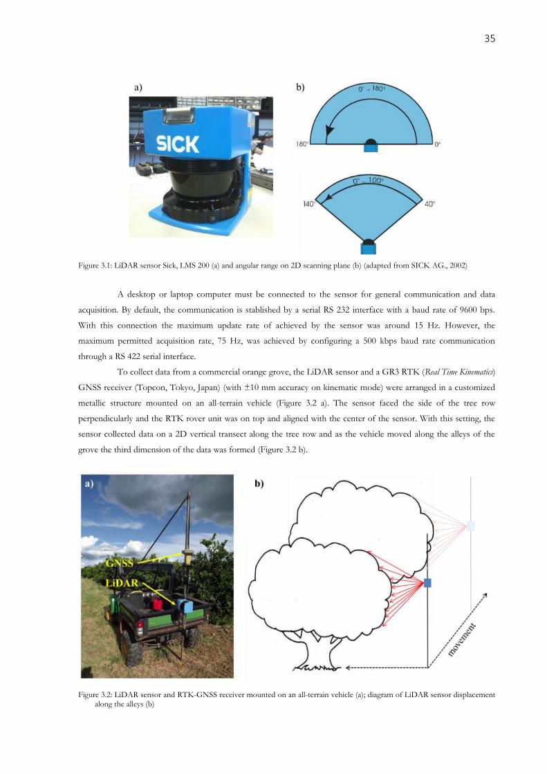
Figure 3.1: LiDAR sensor Sick, LMS 200 (a) and angular range on 2D scanning plane (b) (adapted from SICK AG., 2002)
A desktop or laptop computer must be connected to the sensor for general communication and data
acquisition. By default, the communication is stablished by a serial RS 232 interface with a baud rate of 9600 bps.
With this connection the maximum update rate of achieved by the sensor was around 15 Hz. However, the
maximum permitted acquisition rate, 75 Hz, was achieved by configuring a 500 kbps baud rate communication
through a RS 422 serial interface.
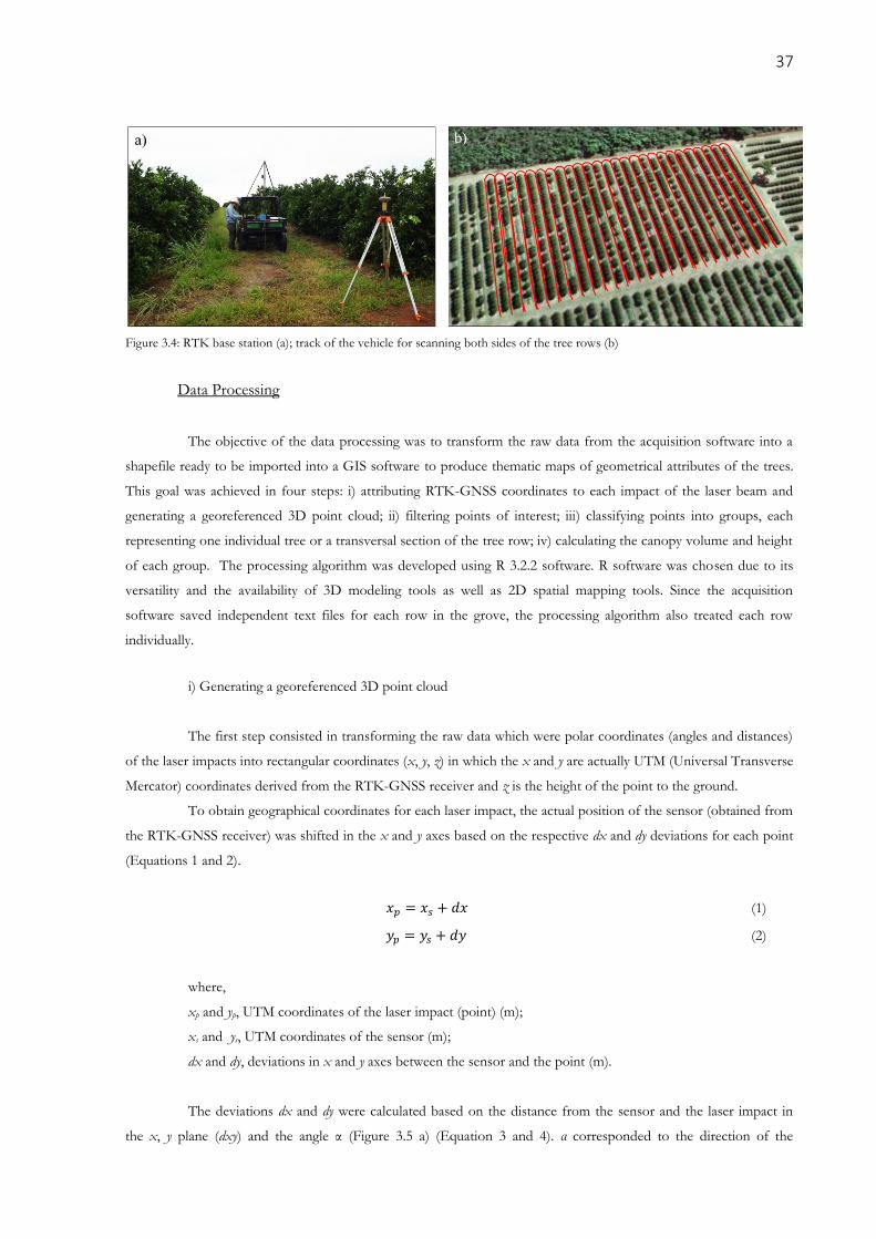
To collect data from a commercial orange grove, the LiDAR sensor and a GR3 RTK (Real Time Kinematics)
GNSS receiver (Topcon, Tokyo, Japan) (with ±10 mm accuracy on kinematic mode) were arranged in a customized
metallic structure mounted on an all-terrain vehicle (Figure 3.2 a). The sensor faced the side of the tree row
perpendicularly and the RTK rover unit was on top and aligned with the center of the sensor. With this setting, the
sensor collected data on a 2D vertical transect along the tree row and as the vehicle moved along the alleys of the
grove the third dimension of the data was formed (Figure 3.2 b).
Figure 3.2: LiDAR sensor and RTK-GNSS receiver mounted on an all-terrain vehicle (a); diagram of LiDAR sensor displacement
along the alleys (b)
36
To acquire data from the LiDAR sensor and the RTK-GNSS receiver synchronously a piece of software
was developed. The chosen programming environment was Processing 2, which uses the JAVA programming
protocol. All communication between the computer and the LiDAR sensor was carried out by a series of messages
that were sent to and from the device following a hexadecimal telegram code (SICK AG. 2003). The communication
with the RTK-GNSS receiver was carried out according to the NMEA (National Marine Electronics Association)
standard. The developed acquisition software started by configuring the communication ports and the baud-rate for
both the LiDAR sensor and the GNSS receiver to stablish communication with the devices. Afterwards, the sensors
was configured, setting its angular resolution and range. Finally, a command was sent to both devices to start
streaming the data.
The final output from the acquisition software was a text file containing information about time, GNSS
location (latitude, longitude and altitude) and distance values from the LiDAR sensor. Figure 3.3 is an example of
one output file where the lines represents each scan of the sensor and the columns labeled as A00, A01, until A180,
represent the measured distance at each angle from the scanner in the 2D transect.
The maximum data acquisition frequency of the GNSS receiver was 10 Hz whereas the LiDAR sensor
was 75 Hz. The software was synchronized with the LiDAR frequency, so during the acquisition process the GNSS
was linearly interpolated and assigned to the LiDAR data so that every scan had a distinct GNSS positioning.
Figure 3.3: Output file from the data acquisition software containing information of the RTK-GNSS receiver and the measured
LiDAR distances in mm
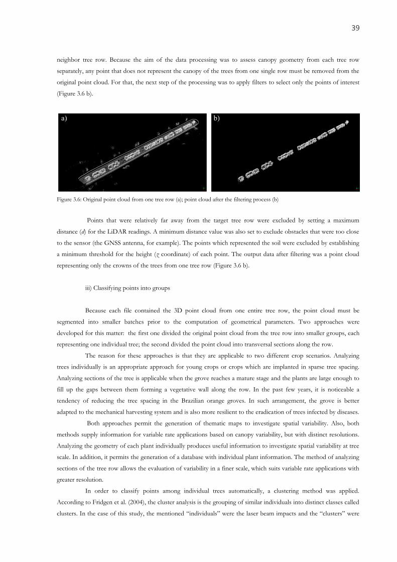
For data acquisition at the groves, the RTK-GNSS base unit was mounted at the highest corner of the
field. Before starting the acquisition, the RTK-GNSS base was kept fixing its position during 30 minutes. The data
collection was only carried out when the correction signal was actually being received by the RTK-GNSS rover unit.
During the measurements, the vehicle moved along the alleys at constant speed, scanning one side of the tree row at
a time (Figure 3.4). The data was saved separately for each tree row.
37
Figure 3.4: RTK base station (a); track of the vehicle for scanning both sides of the tree rows (b)
Data Processing
The objective of the data processing was to transform the raw data from the acquisition software into a
shapefile ready to be imported into a GIS software to produce thematic maps of geometrical attributes of the trees.
This goal was achieved in four steps: i) attributing RTK-GNSS coordinates to each impact of the laser beam and
generating a georeferenced 3D point cloud; ii) filtering points of interest; iii) classifying points into groups, each
representing one individual tree or a transversal section of the tree row; iv) calculating the canopy volume and height
of each group. The processing algorithm was developed using R 3.2.2 software. R software was chosen due to its
versatility and the availability of 3D modeling tools as well as 2D spatial mapping tools. Since the acquisition
software saved independent text files for each row in the grove, the processing algorithm also treated each row
individually.
i) Generating a georeferenced 3D point cloud
The first step consisted in transforming the raw data which were polar coordinates (angles and distances)
of the laser impacts into rectangular coordinates (x, y, z) in which the x and y are actually UTM (Universal Transverse
Mercator) coordinates derived from the RTK-GNSS receiver and z is the height of the point to the ground.
To obtain geographical coordinates for each laser impact, the actual position of the sensor (obtained from
the RTK-GNSS receiver) was shifted in the x and y axes based on the respective dx and dy deviations for each point
(Equations 1 and 2).
𝑥𝑝 = 𝑥𝑠 + 𝑑𝑥 (1)
𝑦𝑝 = 𝑦𝑠 + 𝑑𝑦 (2)
where,
xp and yp, UTM coordinates of the laser impact (point) (m);
xs and ys, UTM coordinates of the sensor (m);
dx and dy, deviations in x and y axes between the sensor and the point (m).
The deviations dx and dy were calculated based on the distance from the sensor and the laser impact in
the x, y plane (dxy) and the angle α (Figure 3.5 a) (Equation 3 and 4). α corresponded to the direction of the
38
measurement in relation to the North, counted clockwise. This angle is the subtraction of 90° from the vehicle
direction in relation to the North (the LiDAR sensor is arranged perpendicularly to the vehicle longitude, facing the
left side). The direction of the vehicle at a given moment is defined by the median values of direction from 30
consecutive points along the vehicle track. Finally, dxy was calculated based on the original polar coordinates of the
laser impacts (distance d and angle β) (Figure 3.5 b) (Equation 5). The z coordinate (point height) is also derived from
the polar coordinates as exposed in Equation 6.
Figure 3.5: dx and dy deviations based on the angle α and dxy (a); dxy based on distance d and angle β (b)
𝑑𝑥 = sen 𝛼 . 𝑑𝑥𝑦 (3)
𝑑𝑦 = cos 𝛼 . 𝑑𝑥𝑦 (4)
𝑑𝑥𝑦 = sen 𝛽 . 𝑑 (5)
𝑧𝑝 = 𝑧𝑠 − (cos 𝛽 . 𝑑) (6)
where,
dxy, the distance between the sensor and the laser impact in the x, y plane (m);
α, angle of the direction of the measurement in relation to the North (degrees);
β, angle from LiDAR scanning (0 to 180°);
d, the distance value from the LiDAR scanning (m);
zp, coordinate z (height) of the point (m);
zs, coordinate z (height) of the sensor (m).
ii) Filtering points of interest
After the transformation from polar to rectangular coordinates, the data is then given by a matrix of three
columns (x, y and z) and n lines, where n is the number of laser impacts. Those data can be visualized in the form of
a 3D point cloud using the CloudCompare 2.6.1 software. Figure 3.6 shows an example of an original point cloud
from a LiDAR scanning in one crop row. It is to be noticed a dotted line along the two sides of the tree row, which
are the laser beam hitting the GNSS antenna. Also, whenever there is a gap between the plants the laser reached the
39
neighbor tree row. Because the aim of the data processing was to assess canopy geometry from each tree row
separately, any point that does not represent the canopy of the trees from one single row must be removed from the
original point cloud. For that, the next step of the processing was to apply filters to select only the points of interest
(Figure 3.6 b).
Figure 3.6: Original point cloud from one tree row (a); point cloud after the filtering process (b)
Points that were relatively far away from the target tree row were excluded by setting a maximum
distance (d) for the LiDAR readings. A minimum distance value was also set to exclude obstacles that were too close
to the sensor (the GNSS antenna, for example). The points which represented the soil were excluded by establishing
a minimum threshold for the height (z coordinate) of each point. The output data after filtering was a point cloud
representing only the crowns of the trees from one tree row (Figure 3.6 b).
iii) Classifying points into groups
Because each file contained the 3D point cloud from one entire tree row, the point cloud must be
segmented into smaller batches prior to the computation of geometrical parameters. Two approaches were
developed for this matter: the first one divided the original point cloud from the tree row into smaller groups, each
representing one individual tree; the second divided the point cloud into transversal sections along the row.
The reason for these approaches is that they are applicable to two different crop scenarios. Analyzing
trees individually is an appropriate approach for young crops or crops which are implanted in sparse tree spacing.
Analyzing sections of the tree is applicable when the grove reaches a mature stage and the plants are large enough to
fill up the gaps between them forming a vegetative wall along the row. In the past few years, it is noticeable a
tendency of reducing the tree spacing in the Brazilian orange groves. In such arrangement, the grove is better
adapted to the mechanical harvesting system and is also more resilient to the eradication of trees infected by diseases.
Both approaches permit the generation of thematic maps to investigate spatial variability. Also, both
methods supply information for variable rate applications based on canopy variability, but with distinct resolutions.
Analyzing the geometry of each plant individually produces useful information to investigate spatial variability at tree
scale. In addition, it permits the generation of a database with individual plant information. The method of analyzing
sections of the tree row allows the evaluation of variability in a finer scale, which suits variable rate applications with
greater resolution.
In order to classify points among individual trees automatically, a clustering method was applied.
According to Fridgen et al. (2004), the cluster analysis is the grouping of similar individuals into distinct classes called
clusters. In the case of this study, the mentioned “individuals” were the laser beam impacts and the “clusters” were
40
the trees. Among several clustering algorithms available, the chosen algorithm was the k-means. This is a common
non-supervised partitioning algorithm, which is available in R software through the stats package. This algorithm
seeks to maximize the similarity between individuals inside the clusters and minimize it between the clusters.
This method requires the desired number of groups prior to the classification or an initial estimation of
the centers of each cluster. After classification, each group should represent one individual tree, so the number of
trees in one row should be known or estimated and then informed to the algorithm. To improve the accuracy of the
classification, the estimation of the centers of each cluster were informed to the algorithm. This estimation was based
on the spacing between the trees and the direction of the row. The algorithm used this information as an initial guess
of the cluster centers. The points were then classified (Figure 3.7) according to their position in space so the
information accounted by the algorithm was the x and y coordinates from each point.
Figure 3.7: The x and y coordinates of a point cloud from orange trees (a); and clustering classification into groups each representing one individual tree (b)
The second approach of grouping the points was based on segmenting the row perpendicularly to its
longitude, creating transversal sections with fixed width and length. The boundary lines of each transect were
automatically drawn using the R package sp which allows delineation of lines and polygons using geographical
information. The first step was to compute a linear regression with the x and y coordinates of the filtered point
cloud. This represented a central longitudinal line of the tree row. A deviation was applied from this central line to
both sides of the row. Finally, the row was segmented lengthwise based on a given distance (Figure 3.8) and the
points within each section were assigned the section identification number.
41
Figure 3.8: Top view of a point cloud; segmentation of the tree row (a); classified points in transversal sections (b)
iv) Calculating canopy volume and height
In order to compute geometrical attributes such as canopy volume, a 3D object was modeled over each
classified point cloud (cluster or section). Two 3D modeling algorithms available in the software R were tested in this
study: the convex-hull (package grDevices); and the alpha-shape (package alphashape3d). Both algorithms were designed to
produce the smallest involucre able to enclose a set of 3D point cloud. The first one produces a convex object and
the second permits an object with concavities. The level of concavity is defined by the index α (higher α produce less
concavity). The canopy volume was automatically retrieved by the algorithm. By its definition, the convex-hull should
produce larger object volumes and probably overestimate the canopy volume since each salient branch from the tree
will pull out the hull structure. On the other hand, the alpha-shape should better suit the irregularities from the canopy
reducing the effect of salient branches on the canopy volume computation, especially by setting a lower α index.
The canopy height was simply obtained by assessing the point of maximum height (z) within each group
(cluster or transversal section). The final output of the processing steps was a GIS shapefile containing the polygons
and the canopy volume and height information for each cluster or section boundaries.
3.3.2. Demonstrating and testing the proposed methods
Assessing the point cloud accuracy
Although the accuracy of the laser sensor is known and considered sufficient to produce accurate point
clouds, the overall data acquisition method and the arrangement of the LiDAR sensor, RTK-GNSS receiver and
vehicle might produce unknown errors over the point cloud. For this reason, a test procedure was carried out to
assess the accuracy of the point cloud generated by the proposed method.
Objects with regular geometry were selected as targets to be scanned by the LiDAR-based system. A
platform carrying the sensor and the RTK-GNSS receiver was designed to run over a rail at constant speed powered
by means of an electric motor. Such a testing set up was develop to minimize the effect of vibration during the data
acquisition. A second scanning over the objects was carried out with the actual all-terrain vehicle mounting the same
equipment as in the real reading in the groves. During the tests the vehicle moved over a leveled lawn.
42
The accuracy of the point cloud was assessed by simply comparing the dimensions of the objects in the
point cloud with the actual dimensions of the objects. The virtual dimensions (from the point clouds) were obtained
using a distance measurement tool available in the CloudCompare software.
Data acquisition in a commercial grove
In order to demonstrate the proposed methods for data acquisition and processing, a 25 ha orange grove
located in the state of São Paulo, Brazil, was scanned. The variety of the trees was “Valencia” grafted to “Swingle”
rootstock. Trees were planted in 2009 and were six years old at the time of this study. The spacing was 2.6 m
between trees and 6.8 m between rows. At the time of the readings, the tree canopies were already touching each
other along the row, partially closing the gaps between them (Figure 3.9). This grove was grown in a rain-fed system.
Figure 3.9: 25 ha commercial orange grove scanned with the laser sensor
The aforementioned equipment and data acquisition method were applied. The vehicle moved along the
alleys at 3.3 m s-1, scanning one side of the tree row at a time. The configuration of the sensor used is shown in Table
3.1.
Due to a 13 m gradient in elevation, this field was implemented with terraces on terrain contours for soil
conservation. The tree rows were planted as straight lines which occasionally crossed over the terraces. The areas
surrounding the terraces were more suited to errors during the readings due to the movement of the vehicle to cross
over them. These areas were subsequently excluded from the analysis.
Table 3.1: Configuration used for the LiDAR sensor
Communication Angle Distance Scan
frequency Protocol Baud Rate Range Resolution Range Resolution
Serial RS 422 500 kbps 0 – 180° 1° 8 m 1 mm 75 Hz
Modeling of 3D objects from the point cloud
As shown during the data processing description, several alternatives can be used during the processing of
a point cloud in order to model a 3D object over the points. To compare these possibilities, different methods to
43
create 3D objects were applied over a set of point clouds from 25 individual orange trees. These trees were extracted
from the original point cloud obtained from the entire field. The selection of these trees aimed to capture different
canopy sizes. The 3D objects were modeled over each plant individually and over transversal sections of 0.86 m, 0.52
m, 0.37 m and 0.26 m wide, which were equivalent to dividing the trees into three, five, seven or ten transversal
parts, respectively. The convex-hull and the alpha-shape algorithms were applied. Variations over the alpha-shape were
also tested by setting the index α to 0.25, 0.50 or 0.75.
The tree volumes from each method were compared against each other. The volume of each
individual tree was also computed by two methods based on manual measurement of the canopy dimensions. In the
first manual method, referred here as “cylinder-fit”, the canopy volume of a citrus tree is considered as two-thirds
the volume of the smallest cylinder able to enclosure the tree (Mendel, 1956). The second method, referred here as
“cube-fit”, is the current method adopted in most of the Brazilian groves. The volume of the tree is simply given by
the volume of a cube, which encloses the canopy. The dimension of this cube is given by multiplying the two widths
of the canopy (along the row axis and perpendicular to the row axis) with the height of the canopy. The dimensions
of the canopy for the manual methods were measured from the point cloud of each tree by using a distance
measurement tool available in the CloudCompare software.
These processing methods were also applied over a point cloud from a 26 m segment of a tree row. 3D
visualization of the modeling and general observations over the results were carried out.
Mapping of canopy volume and height in a commercial orange grove
To produce a map of canopy volume from the scanned grove, the point cloud was processed in two
different ways. The first method was based on computing the canopy volume for each individual tree (cluster) and
applying the alpha-shape algorithm with the index α set to 0.75. The second approach was based on dividing the rows
into sections of 0.26 m width and applying the convex-hull algorithm. These setting were chosen after evaluating the
results from the previous analysis, which tested several options for modeling the tree’s canopies.
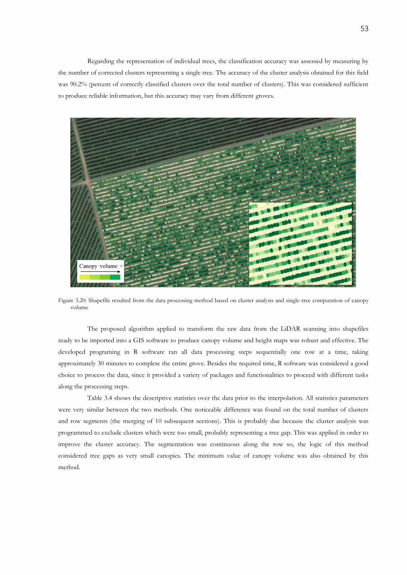
Because the trees were partially touching each other, some error in the cluster classification was expected.
The accuracy of this classification was assessed by visually recognizing 678 trees from the point cloud and comparing
them with the outcome of the cluster classification using the CloudCompare software.
The canopy volume and height maps were produced by importing the shapefiles from the data processing
output into the QGIS 2.10 software. A map of points, each representing one tree or a transversal section of the row,
was created by generating a centroid point within each polygon. Points close up to 10 m to the field boundary were
excluded. Due to maneuvering of the vehicle the point cloud might lose accuracy and the clustering algorithm was
more suited to errors in that region. In addition, the points within a 15 m buffer around the terraces in the field were
excluded. The point cloud lost accuracy in those regions because of the movement of the vehicle to cross over the
terraces.
To produce the final canopy volume and height maps, the points that represented each tree or section
were interpolated in a regular pixel grid in order to produce a continuous surface across the grove. Prior to the
interpolation, the values from the row sections were converted into values equivalent to individual trees, otherwise
the final map would represent volume of row sections and not of individual trees. Therefore, sections were merged
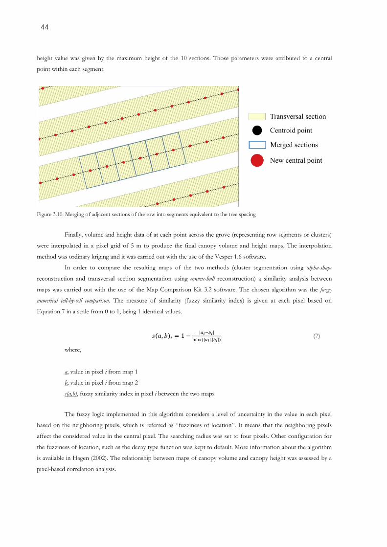
in groups of 10 along the row forming segments of 2.6 m of length, which was equivalent to the tree spacing (Figure
3.10). The canopy volume of each segment was given by adding the volume of the 10 sections inside it and the
44
height value was given by the maximum height of the 10 sections. Those parameters were attributed to a central
point within each segment.
Figure 3.10: Merging of adjacent sections of the row into segments equivalent to the tree spacing
Finally, volume and height data of at each point across the grove (representing row segments or clusters)
were interpolated in a pixel grid of 5 m to produce the final canopy volume and height maps. The interpolation
method was ordinary kriging and it was carried out with the use of the Vesper 1.6 software.
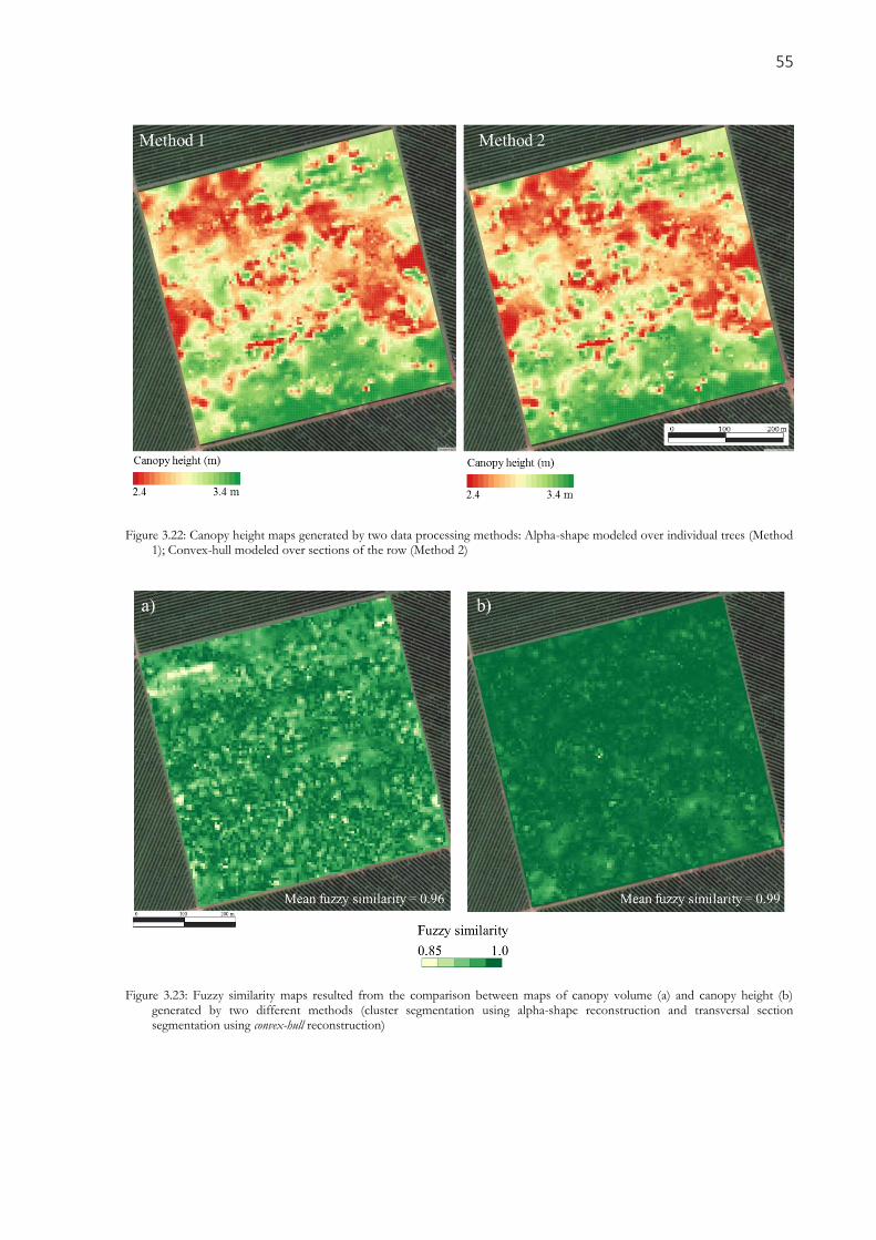
In order to compare the resulting maps of the two methods (cluster segmentation using alpha-shape
reconstruction and transversal section segmentation using convex-hull reconstruction) a similarity analysis between
maps was carried out with the use of the Map Comparison Kit 3.2 software. The chosen algorithm was the fuzzy
numerical cell-by-cell comparison. The measure of similarity (fuzzy similarity index) is given at each pixel based on
Equation 7 in a scale from 0 to 1, being 1 identical values.
𝑠(𝑎, 𝑏)𝑖 = 1 −|𝑎𝑖−𝑏𝑖|
max (|𝑎𝑖|,|𝑏𝑖|) (7)
where,
a, value in pixel i from map 1
b, value in pixel i from map 2
s(a,b), fuzzy similarity index in pixel i between the two maps
The fuzzy logic implemented in this algorithm considers a level of uncertainty in the value in each pixel
based on the neighboring pixels, which is referred as “fuzziness of location”. It means that the neighboring pixels
affect the considered value in the central pixel. The searching radius was set to four pixels. Other configuration for
the fuzziness of location, such as the decay type function was kept to default. More information about the algorithm
is available in Hagen (2002). The relationship between maps of canopy volume and canopy height was assessed by a
pixel-based correlation analysis.
45
3.4. Results and Discussion
3.4.1. Point cloud generation - laboratory testing
The accuracy of the point cloud derived from the developed MTLS was assessed by using template
objects as targets for scanning. Figure 3.11 shows the point clouds from a cylinder, a body of cone, a square, triangle
and circle shaped objects scanned by the MTLS mounted on the all-terrain vehicle (the same data acquisition setting
applied in the groves). These results seems coherent by a visual assessment. The same objects were also scanned with
the MTLS mounted on a platform running over a rail.
Figure 3.11: Point clouds from objects scanned by a mobile terrestrial laser scanner mounted on an all-terrain vehicle; cylinder (a),
body of cone (b), square (c), triangle (d) and circle (e)
The dimensions of the objects obtained by the two scanning systems are viewed in Table 3.2. It should be
noticed that, in order to simplify the design of such tests, the accuracy of the point cloud was evaluated based on the
obtained dimensions of the objects and not by assessing the actual positioning error of each laser beam impact (as it
would be ideal). Generally, both scanning systems provided very similar dimensions to the actual dimensions of the
objects, with, as expected, slightly better results when the MTLS was running over the rail. The overall average
difference between the laser measurements and the actual dimensions of the objects was 0.69 cm, reaching a
maximum of 5.77 cm (‘b’ dimension of the square with the MTLS mounted on the vehicle). The surface area and the
volume of the objects calculated from these measurements were also close to the actual areas and volumes.
46
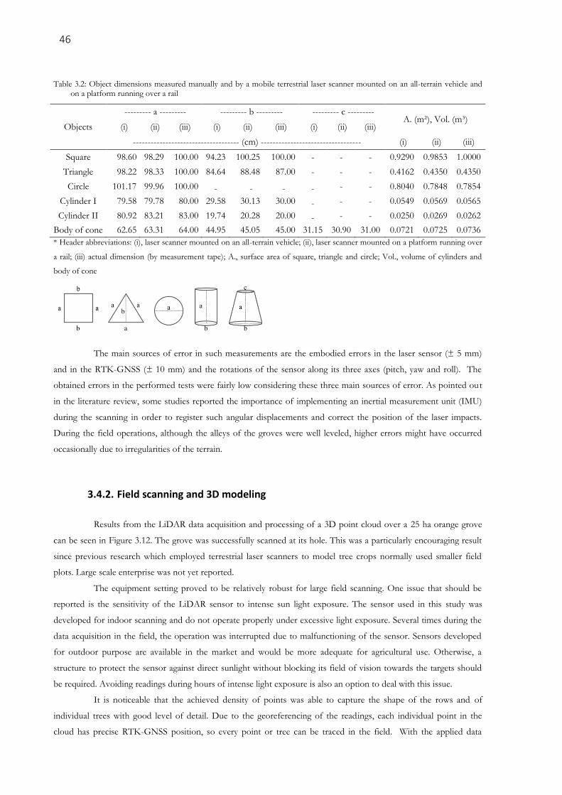
Table 3.2: Object dimensions measured manually and by a mobile terrestrial laser scanner mounted on an all-terrain vehicle and on a platform running over a rail
Objects
--------- a --------- --------- b --------- --------- c --------- A. (m²), Vol. (m³)
(i) (ii) (iii) (i) (ii) (iii) (i) (ii) (iii)
------------------------------------ (cm) ---------------------------------- (i) (ii) (iii)
Body of cone 62.65 63.31 64.00 44.95 45.05 45.00 31.15 30.90 31.00 0.0721 0.0725 0.0736
* Header abbreviations: (i), laser scanner mounted on an all-terrain vehicle; (ii), laser scanner mounted on a platform running over
a rail; (iii) actual dimension (by measurement tape); A., surface area of square, triangle and circle; Vol., volume of cylinders and
body of cone
The main sources of error in such measurements are the embodied errors in the laser sensor (± 5 mm)
and in the RTK-GNSS (± 10 mm) and the rotations of the sensor along its three axes (pitch, yaw and roll). The
obtained errors in the performed tests were fairly low considering these three main sources of error. As pointed out
in the literature review, some studies reported the importance of implementing an inertial measurement unit (IMU)
during the scanning in order to register such angular displacements and correct the position of the laser impacts.
During the field operations, although the alleys of the groves were well leveled, higher errors might have occurred
occasionally due to irregularities of the terrain.
3.4.2. Field scanning and 3D modeling
Results from the LiDAR data acquisition and processing of a 3D point cloud over a 25 ha orange grove
can be seen in Figure 3.12. The grove was successfully scanned at its hole. This was a particularly encouraging result
since previous research which employed terrestrial laser scanners to model tree crops normally used smaller field
plots. Large scale enterprise was not yet reported.
The equipment setting proved to be relatively robust for large field scanning. One issue that should be
reported is the sensitivity of the LiDAR sensor to intense sun light exposure. The sensor used in this study was
developed for indoor scanning and do not operate properly under excessive light exposure. Several times during the
data acquisition in the field, the operation was interrupted due to malfunctioning of the sensor. Sensors developed
for outdoor purpose are available in the market and would be more adequate for agricultural use. Otherwise, a
structure to protect the sensor against direct sunlight without blocking its field of vision towards the targets should
be required. Avoiding readings during hours of intense light exposure is also an option to deal with this issue.
It is noticeable that the achieved density of points was able to capture the shape of the rows and of
individual trees with good level of detail. Due to the georeferencing of the readings, each individual point in the
cloud has precise RTK-GNSS position, so every point or tree can be traced in the field. With the applied data
47
acquisition configuration (75 Hz scanning frequency at 3.3 m s-1 speed) the distance between each scan was around 4
cm. A total of approximately 2.3 million points were acquired for each row (approximately 12,100 point per plant).
The total grove accounted for approximately 175 million points, which corresponds to approximately 700 points per
m². Airborne LiDAR scanning applied over urban or forest areas usually produces point clouds with 0.5 to 5 points
per m². Escolà et al. (2015) reported a density of 8,000 points per m² using a multi-echo LiDAR device on a MTLS
on an olive grove.
To achieve a proper density of points in the scanned orange grove the vehicle movement was set to a
relatively low speed resulting in a low working efficiency for data acquisition. Nevertheless, this speed is compatible
with several mechanical operations in the grove such as spraying, which means that the LiDAR-based scanning
system could be attached to the machines in the field to collect data while performing other agricultural operations.
Figure 3.12: Point cloud derived from the developed terrestrial laser scanning system in a 25 ha commercial orange grove
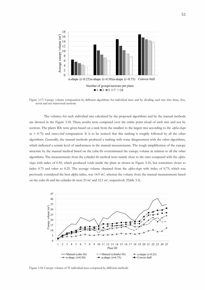
The results of the proposed 3D modeling algorithms applied to a segment of tree row of 26 m is showed
in Figure 3.13. It is noticeable how the convex-hull model apparently produced larger objects, which occurs because
salient branches enlarges the hull structure. As expected, salient branches were better represented by the alpha-shape
algorithm with lower α index. However, the index α should be appropriately set (not too high neither too low). A low
index might produce disconnected structures forming holes inside the canopy, which is not desirable. Because this
algorithm permits the representation of concave structures, it is reasonable to consider the alpha-shape a suited model
for representing the tree canopy. Likewise, it is noticeable that slicing the row into transversal sections instead of
maintaining the tree as a whole also helped the representation of the canopies with greater level of detail. The
48
segmentation of the trees was particularly important in the convex-hull model, because it reduced the effect of over
estimation caused by outer branches on the tree. This issue was more severe when the model was created over the
entire plant. The importance of segmenting the point cloud when applying the convex-hull algorithm to estimate
volume was also evidenced by Auat Cheein et al. (2015).
Figure 3.13: Convex-hull and alpha-shape algorithms to model orange trees by two approaches: clusters (individual tree) and transversal sections of the row (0.26 m wide)
However, when slicing the trees to produce 3D models of continuous canopies a problem with the alpha-
shape algorithm was evidenced. While the algorithm produced desirable concavities on the outer part of the canopy,
49
which helped detailing the silhouette of the canopy, it also created undesirable depressions in the transversal slicing
plane and in the bottom of the trees (Figure 3.14). When all the sections were put together, the concavities in the
transversal wall of the sections produced voids, which affected the final computation of canopy volume. The voids
between sections were also present in the convex-hull models but they were considered insignificant (Figure 3.15_.
They are inherent to the approach of slicing the rows and are directly related with the scanning frequency during the
data acquisition (which determines the spacing between scans). Because of the high scanning frequency, the space
between each scan was very narrow and so was the voids between the convex-hull objects (Figure 3.15). Thus, the
convex-hull algorithm was considered better than the alpha-shape to represent transversal sections of the row.
Figure 3.14: Detail of the convex-hull and alpha-shape modeled over a single 0.26 m wide transversal section of a tree row
Figure 3.15: Top view of the convex-hull modeling over transversal sections of an orange tree row
Nevertheless, the alpha-shape algorithm remained a better option when the model was applied over the
entire tree. The best index α should be the one which does not produce voids inside the canopy. In the Figure 3.16 it
is noticeable that this result was obtained when the index α was set to 0.75.
50
Figure 3.16: 3D canopy structure of a single tree modeled by different algorithms
The results from the measurements of 25 individual trees extracted from the scanned grove also
confirmed the observations made from the previous analysis (Table 3.3). The convex-hull model resulted in the highest
canopy volume, followed by the alpha-shape with higher index α. The canopy volume also decreased as the number of
slices of the trees increased. This decrease is higher in alpha-shape algorithm (Figure 3.17), probably due to the
increase of voids between sections as mentioned. When using the alpha-shape algorithm, there was a 2-fold range in
the volume computation by computing the volume of the tree as a whole or by dividing it into 10 sections (Table
3.3).
Table 3.3: Mean canopy volume of 25 individual trees by different methods and by dividing the trees into different number of sections
Method / Algorithm
Number of sections per tree
1 3 5 7 10
Mean canopy volume of 25 individual trees (m³)
Manual (cube-fit) 23.01 - - - -
Manual (cilinder-fit) 12.15 - - - -
Convex-hull 16.95 15.61 14.85 14.29 13.67
α-shape (α =0.75) 14.92 12.12 10.31 8.89 7.58
α-shape (α =0.50) 12.66 10.21 8.43 7.19 5.92
α-shape (α =0.25) 6.43 5.51 4.89 4.28 3.45
51
Figure 3.17: Canopy volume computation by different algorithms for individual trees and by dividing each tree into three, five, seven and ten transversal sections
The volumes for each individual tree calculated by the proposed algorithms and by the manual methods
are showed in the Figure 3.18. These results were computed over the entire point cloud of each tree and not by
sections. The plants IDs were given based on a rank from the smallest to the largest tree according to the alpha-shape
(α = 0.75) and convex-hull computation. It is to be noticed that this ranking is roughly followed by all the other
algorithms. Generally, the manual methods produced a ranking with some disagreement with the other algorithms,
which indicated a certain level of randomness in the manual measurements. The rough simplification of the canopy
structure by the manual method based on the cube-fit overestimated the canopy volume in relation to all the other
algorithms. The measurements from the cylinder-fit method were mainly close to the ones computed with the alpha-
shape with index of 0.50, which produced voids inside the plant as shown in Figure 3.16, but sometimes closer to
index 0.75 and other to 0.25. The average volume obtained from the alpha-shape with index of 0.75, which was
previously considered the best alpha index, was 14.9 m³, whereas the volume from the manual measurements based
on the cube-fit and the cylinder-fit were 23 m³ and 12.1 m³, respectively (Table 3.3).
Figure 3.18: Canopy volume of 25 individual trees computed by different methods
52
The difference in canopy volume obtained from different methods evidenced the importance of the
adoption of a reference method. The choice of the best method based on the one which is more close to a reference
is simply not possible since the “real” canopy volume is not known and cannot be measured without the
establishment of a standardized method. At this stage, it is reasonable to consider that the method of canopy volume
computation based on the terrestrial laser scanner and 3D modeling is clearly more capable of capturing the
geometry of the canopy than the current available manual methods. The proposed methods are also applicable in the
field and, for those reasons, could be adopted as a new standard method of canopy volume computation.
These first considerations about the 3D modeling methods led to the conclusions that, among the tested
options, the best algorithm for modeling the canopy of individual trees was the alpha-shape with index α set to 0.75,
because it permits the representation of salient structures from the canopy while keeping the canopy as a solid
without voids inside it. The convex-hull algorithm was a better option for modeling of sections of the trees, because it
produced minimum voids between the sections. The weakness of this algorithm, which is overestimating the
structure in outer parts of the tree, is less relevant when the tree is divided into sections.
3.4.3. Mapping of canopy volume and height
The final canopy volume and height maps were produced by two methods: by classifying the point cloud
into individual tress (cluster) and subsequently applying the alpha-shape algorithm (α = 0.75); and by dividing the rows
into sections of 0.26 m wide and further applying the convex-hull algorithm to model the canopies. The two data
processing methods produced shapefiles of polygons where each polygon contained the information of canopy
volume and height computed by the algorithms (Figure 3.19 and 3.20). The slicing of the rows produced
approximately ten polygons per tree (prior to interpolation every ten subsequent section were merged together to
produce the final map). Inside each polygon approximately 6 laser scans were found.
Figure 3.19: Shapefile resulted from data processing according to the method based on segmenting the row into transversal section
53
Regarding the representation of individual trees, the classification accuracy was assessed by measuring by
the number of corrected clusters representing a single tree. The accuracy of the cluster analysis obtained for this field
was 90.2% (percent of correctly classified clusters over the total number of clusters). This was considered sufficient
to produce reliable information, but this accuracy may vary from different groves.
Figure 3.20: Shapefile resulted from the data processing method based on cluster analysis and single-tree computation of canopy volume
The proposed algorithm applied to transform the raw data from the LiDAR scanning into shapefiles
ready to be imported into a GIS software to produce canopy volume and height maps was robust and effective. The
developed programing in R software ran all data processing steps sequentially one row at a time, taking
approximately 30 minutes to complete the entire grove. Besides the required time, R software was considered a good
choice to process the data, since it provided a variety of packages and functionalities to proceed with different tasks
along the processing steps.
Table 3.4 shows the descriptive statistics over the data prior to the interpolation. All statistics parameters
were very similar between the two methods. One noticeable difference was found on the total number of clusters
and row segments (the merging of 10 subsequent sections). This is probably due because the cluster analysis was
programmed to exclude clusters which were too small, probably representing a tree gap. This was applied in order to
improve the cluster accuracy. The segmentation was continuous along the row so, the logic of this method
considered tree gaps as very small canopies. The minimum value of canopy volume was also obtained by this
method.
54
Table 3.4: Descriptive statistics of canopy volume and height for the two methods
Canopy variable Method* Mean Minimum Maximum Coef. of
variation Observations
----- m³ (volume) or m (height) -----
Volume 1 11.94 1.29 26.50 0.20 9119
2 12.15 0.25 26.30 0.21 9669
Height 1 2.85 1.03 3.80 0.09 9119
2 2.86 0.95 3.80 0.09 9669
*Method 1: Alpha-shape modeling over individual trees
**Method 2: Convex-hull modeling over sections of the row
The two methods produced similar results for canopy volume and height. The final maps were visually
similar (Figure 3.21 and 3.22). The similarity between the maps assessed by the fuzzy similarity index was higher for
the canopy height (fuzzy similarity index = 0.99) than for the canopy volume (Figure 3.23). This is because both
methods applied the same rational to compute the height. The height of each cluster or section of the row was equal
to the height of the point with maximum height inside the cluster or section. The canopy volume maps were
computed by two different algorithms, so the fuzzy comparison resulted in slightly lower index (fuzzy similarity
index = 0.96).
Some relation between height and canopy volume was also expected. This correlation was higher when
the two parameters were computed using the cluster analysis (r = 0.71). The grouping of sections along the row did
not necessarily match with individual plants, so the correlation of height and volume was not as high (r = 0.61).
Generally, both methods resulted similarly. They were both able to represent the spatial variability of
canopy geometry in the grove. These maps are useful information for site-specific management, providing
information for variable rate applications or to divide the field into management zones.
Figure 3.21: Canopy volume maps generated by two data processing methods: Alpha-shape modeled over individual trees (Method 1); Convex-hull modeled over sections of the row (Method 2)
55
Figure 3.22: Canopy height maps generated by two data processing methods: Alpha-shape modeled over individual trees (Method 1); Convex-hull modeled over sections of the row (Method 2)
Figure 3.23: Fuzzy similarity maps resulted from the comparison between maps of canopy volume (a) and canopy height (b) generated by two different methods (cluster segmentation using alpha-shape reconstruction and transversal section segmentation using convex-hull reconstruction)
56
3.5. Conclusions
A methodology for 3D modeling and canopy geometry computation for orange groves was developed
using a terrestrial georeferenced laser scanning system based on a LiDAR sensor. Variations over the data processing
and 3D modeling algorithms were demonstrated and compared.
The method of data acquisition based on MTLS and 3D point cloud generation proved to produce
reliable georeferenced point clouds of a commercial orange grove. The data acquisition set up was robust for large
field scanning and could be implemented on current agricultural operations in the groves.
The convex-hull and alpha-shape (α = 0.75) 3D modeling algorithms worked best when implemented over
transversal sections of the row and over individualized plants, respectively. Nevertheless, the canopy volume and
height maps produced by these two methods showed similar spatial variability in the evaluated grove. However,
varying the type of segmentation of the cloud and the 3D modeling algorithms resulted in different values of canopy
volume indicating the need for a reference method to be adopted. Nevertheless, the mapping of canopy volume and
height by either cluster or section of the row resulted in similar maps.
The proposed data acquisition and processing systems were able to produce useful information for
precision agriculture management. The LiDAR scanning and the proposed data processing and mapping reproduced
the spatial variability in the grove in the format of thematic maps that can be used for variable rate applications and
to guide management zones delineations within the grove. All the software used is open-source and freely available
to any user.
References
AUAT CHEEIN, F. A. et al. Real-time approaches for characterization of fully and partially scanned canopies in
groves. Computers and Electronics in Agriculture, Amsterdam, v. 118, p. 361–371, out. 2015.
AUAT CHEEIN, F. A.; GUIVANT, J. SLAM-based incremental convex hull processing approach for treetop
volume estimation. Computers and Electronics in Agriculture, Amsterdam, v. 102, p. 19–30, mar. 2014.
COLAÇO, A. F.; MOLIN, J. P. Variable rate fertilization in citrus: a long term study. Precision Agriculture,
Dordrecht, 13 maio 2016.
DEL-MORAL-MARTÍNEZ, I. et al. Georeferenced Scanning System to Estimate the LeafWall Area in Tree Crops.
Sensors, New York, v. 15, n. 4, p. 8382–8405, 2015.
DEL-MORAL-MARTÍNEZ, I. et al. Mapping Vineyard Leaf Area Using Mobile Terrestrial Laser Scanners: Should
Rows be Scanned On-the-Go or Discontinuously Sampled? Sensors, New York, v. 16, n. 1, p. 119, 2016.
ESCOLÀ, A. MARTINEZ-CASASNOVAS, J. A.; RUFAT, J. ARBONÉS, A.; SANZ, R.; SEBÉ, F.; ARNÓ, J.;
MASIP, J.; PASCUAL, M.; GREGORIO, E.; RIBES-DASI, M.; VILLAR, J. M.; ROSELL-POLO, J. R. A
monile terrestrial laser scanner for tree crops: point cloud generation, information, extraction and validation in
an intensive olive orchard. In: EUROPEAN CONFERENCE ON PRECISION AGRICULTURE, 10., 2015,
Tel Aviv. Proceedings... Wageningen: Wageningen Academic Publishers, 2015. p. 337 - 344.
FRIDGEN, J. J. et al. Management zone analyst (MZA): Software for subfield management zone delineation.
Agronomy Journal, Madison, v. 96, p. 100–108, 2004.
HAGEN, A. Multi-method assessment of map similarity. In: AGILE CONFERENCE ON GEOGRAPHIC
INFORMATION SCIENCE, 5., 2002, Palma. Proceedings… 2002.
57
LEE, K. H.; EHSANI, R. A laser scanner based measurement system for quantification of citrus tree geometric.
Applied Engineering in Agriculture, St. Joseph, v. 25, n. 5, p. 777–788, 2009.
MENDEL, K. Rootstock-scion relationships in Shamouti trees on light soil. Ktavim, Rehovot, v.6, p.35-60, 1956.
ROSELL, J. R. et al. Obtaining the three-dimensional structure of tree orchards from remote 2D terrestrial LIDAR
scanning. Agricultural and Forest Meteorology, Amsterdam, v. 149, n. 9, p. 1505–1515, set. 2009.
ROSELL, J. R.; SANZ, R. A review of methods and applications of the geometric characterization of tree crops in
agricultural activities. Computers and Electronics in Agriculture, Amsterdam, v. 81, p. 124–141, fev. 2012.
SICK AG. Quick Manual for LMS communication setup - Hardware setup and measurement mode configuration.
Version 1.1. 2002
SICK AG. Telegrams for Operating/Configuring the LMS2XX Laser Measurement Systems. Firmware version
V.2.10/X1.14. 2003.
TUMBO, S. D. et al. Investigation of laser and ultrasonic ranging sensors for measurements of citrus canopy
volume. Applied Engineering in Agriculture, St. Joseph, v. 18, n. 3, p. 367–372, 2002.
WEI, J.; SALYANI, M. Development of a laser scanner for measuring tree canopy characteristics: phase 1. Prototype
development. Transactions Of The Asabe, St. Joseph, v. 47, n. 6, p. 2101–2108, 2004.
58
59
4. CANOPY VOLUME AND HEIGHT SPATIAL VARIABILITY AND SITE-SPECIFIC
APPLICATIONS IN COMMERCIAL ORANGE GROVES
ABSTRACT
One key aspect when designing new site-specific management practices is the comprehensive understanding over the spatial variability of the fields. LiDAR technology trough mobile terrestrial laser scanners (MTLS) is able to provide with useful information about spatial variability of tree crop geometry. However, a general characterization of canopy volume and height variability in orange crops was not yet broadly explored by research. Once canopy variability is acknowledged, the sensor-based or map-based variable rate application of inputs is a suited solution to deal with canopy size variability. The relationship between canopy geometry and other relevant variables to the variability of crop performance should also be investigated in order to enhance site-specific practices. Therefore, the objective of this study was to characterize the variability of canopy volume and height in commercial orange groves in Brazil. In addition, it aimed to investigate the relationship between geometrical parameters of the trees with soil attributes and historical fruit yield. Five commercial orange orchards in São Paulo, Brazil, ranging from 10 to 25 ha, were selected to be scanned with a develop MTLS system based on LiDAR sensor. The canopy volume and height were computed for every 0.25 m section of the rows. The values of canopy volume and height of every ten adjacent sections were merged together and then interpolated into a 5 m pixel grid. A descriptive statistics and geostatiscal analyses were carried out to investigate the variability in canopy geometry. The input savings from sensor-based variable rate applications were estimated. Three out of the five initial groves were selected and their historical yield and soil map database were investigated. A pixel-based correlation analysis was carried out between the canopy geometry, yield and soil maps. One final analysis was performed in order to verify whether canopy geometry maps are effective on guiding the delineation of management zones within the groves. The selected groves were divided into three zones of different tree sizes. The mean values of historical yield and soil attribute were assessed for each zone and compared. The canopy volume and height of 0.25 m sections showed a coefficient of variation ranging from 31 to 41% and from 15 to 24%, respectively. The potential input savings provided by sensor-based variable rate applications were around 40% when compared to constant rate application base on the grove’s maximum canopy volume. The canopy volume and height maps showed that these variables might significantly vary within short distances, but also large consistent regions of different tree sizes were recognized. The historical yield and soil database from the three selected groves showed that grove 1 was generally less variable with less temporal consistency then groves 2 and 3. Canopy geometry was more strongly related with yield and soil variables in groves 2 and 3 (R² up to 0.72). Nevertheless, the use of canopy volume and height information was successful on distinguishing zones of different yield performances and soil characteristics in all three groves. Given the variability found on canopy volume and height, this study proved the benefits of MTLS used for site-specific practices in commercial orange groves.
A general evaluation of the spatial variability in these groves indicates that the youngest grove, grove 1,
presented less variability in yield, soil attributes and canopy volume. The variability found in the maps was not very
consistent and there was little resemblance between them. As discussed in the first section of the results, the canopy
volume showed a frequency distribution close to normality and a weak spatial dependence indicating a certain level
of randomness of the spatial variability of canopy volume. Grove 3 presented higher variability in soil conditions,
significant yield variability and consistency along the years. The canopy geometry variation usually matched the
variability found in soil and yield. Grove 2 showed intermediate results. Significant variation was found in altitude
and soil attributes, which was reflected in yield variability in some years. The canopy volume and height maps were
not strongly correlated with yield. The canopy volume histograms in groves 2 and 3 were more asymmetrical than in
grove 1, presenting a slightly stronger spatial dependence than grove 1, indicating more consistent regions with
distinct canopy sizes in those groves.
Some studies in Florida have shown strong correlations between orange fruit yield and ultrasonically
measured canopy volume. However, different methods were applied in order to correlate these two variables. The
highest correlation was reported by Mann, Schumann and Obreza (2010). They reached an R² of 0.85 when
correlating the canopy volume and yield from 30 selected locations from a 10 ha orange grove. Zaman, Schumann
and Hostler (2006) divided an orange grove into forty 0.4 ha plots and got an R² of 0.80 by applying a linear
correlation over data from twenty out of the forty plots (the other half was used as a validation data-set). In the same
grove, Schumann et al. (2006a) correlated yield and canopy volume using the data from all plots and got an R² of
0.64. The canopy height was slightly less correlated (R² = 0.54) with yield than canopy volume. In the present work,
the canopy height was also less correlated with yield and soil attributes than canopy volume. Those groves in Florida
presented significantly higher variability in canopy volume than the Brazilian groves evaluated in this study. The
coefficient of variation of canopy volume in the study of Mann, Schumann and Obreza (2010) was 54%. Besides, the
approach employed by the present study was a pixel-based correlation between maps, which might have contributed
82
to lower correlations. Schumann et al. (2006a) reported that the variability found in canopy volume was much higher
than yield variability because the method of yield mapping do not allow the yield estimation on a single-tree basis as
the ultrasonic sensor does for canopy volume. Nevertheless, visual resemblance between canopy volume and yield
maps was pointed out by Zaman, Schumann and Hostler (2006) and Mann, Schumann and Obreza (2010).
The correlation between canopy geometry and yield or soil attributes might indicate whether canopy
geometry is a suitable parameter to guide management zones delineation in a given grove. Figure 4.15 shows the
cluster classification of the groves into three zones based on the canopy volume (canopy volume was chosen over
canopy height due to its higher correlations with other variables). The classification in grove 3 produced continuous
zones matching with spatial patterns viewed in soil and yield maps. The resulting zones were more diffuse in groves
1 and 2. The classification of canopy volume in grove 2 resembled the elevation, soil attributes and some yield maps.
Regarding grove 1, the classification of the canopy volume, as the canopy volume maps itself, did not clearly match
any of the yield or soil maps in a visual assessment.
Figure 4.15: Classification of orange groves into different tree size zones
The mean values of each variable in the database (historical yield and soil attributes) were computed for
each canopy volume zone (Table 4.11). As expected, zones with large trees were found in sites with higher clay and
organic matter content. The soil ECa was also higher in those regions, with the exception of grove 3, where the
higher ECa was found in the zone with smaller trees (in that grove high ECa is related to bad soil drainage).
Regarding the yield in each zone, in a few cases some illogical results were found where the highest yield occurred in
the zones with medium (grove 2 in 2013 and grove 3 in 2010) or small trees (grove 3 in 2009). This shows that the
classification was not effective in those cases, probably due to the fact that the canopy volume was measured in 2015
and did not reflect the yield variability in the past or because the spatial variability in these years was unusual.
83
Table 4.11: Mean values of canopy volume, yield and soil attributes in three zones delineated based on canopy volume
Grove Canopy volume zones
Canopy volume
Yield (1)*
Yield (2)*
Yield (3)*
Yield (4)*
Yield (5)*
Yield (6)*
Eca Clay
content O. M. Elev.
(m³) (Mg ha-1) (mS m-1) (%) (%) (m)
1
Large 13.58 a 14.00 a 35.11 a 39.10 a 42.09 a - - 2.53 a 17.26 a 13.93 a 638.02 a
Medium 12.14 b 13.94 a 34.73 b 37.55 b 41.24 b - - 2.44 b 16.86 b 13.68 b 637.60 b
Small 10.79 c 13.78 b 33.21 c 36.52 c 39.99 c - - 2.36 c 16.41 c 13.62 b 637.50 b
2
Large 44.93 a 19.65 a 35.44 a 20.52 a 45.85 a 68.91 a 47.05 b 4.93 a 35.02 a 2.43 a 747.10 c
Medium 39.51 b 17.80 b 32.04 b 20.07 b 45.46 b 65.94 b 47.68 a 4.35 b 31.81 b 2.37 b 749.20 b
Small 32.94 c 16. 86 c 30.22 c 18.83 c 44.18 c 58.86 c 44.98 c 3.95 c 28.85 c 2.33 c 749.70 a
3
Large 42.91 a 13.36 a 21.09 b 20.98 b 52.82 a 62.09 a 42.39 a 0.90 b 14.43 b 1.78 a 766.50 a
Medium 35.52 b 12.23 b 21.28 b 23.80 a 48.45 b 58.73 b 39.48 b 0.92 b 14.74 a 1.69 b 765.80 b
Small 25.54 c 10.64 c 21.80 a 21.24 b 29.76 c 41.63 c 28.97 c 1.91 a 13.42 c 1.65 c 763.50 c
* In grove 1, yield (1) to (4) represent yields from 2012 until 2015 sequentially. In grove 2 and 3, yield (1) to (6) represent yields from 2008 until 2013 sequentially ** Means with the same letter within columns in each grove are not significantly different according to the Tukey test (p > 0.001) *** Header abbreviations: ECa, soil electrical conductivity in 0.3 m depth; O.M., organic matter; Elev., elevation
Nevertheless, practically all variables differed significantly (p > 0.001) between zones in the three groves.
Mann, Schumann and Obreza (2010) obtained similar results by classifying an orange grove into five zones based on
canopy volume. These results indicate that the canopy volume map can provide zones where soil and historical yield
are different. Therefore, the canopy volume map can be used in order to guide zones delineation for different
management. Management zones are usually delineated based on the combination of several layers of information.
In this case, all available variables should be considered as management zones indicators. However, in the absence of
a large database, the canopy volume alone can help revealing zones of different soil and yield performance.
The establishment of management zones based on canopy volume does not mean that application rates
must be kept constant inside each zone. As shown in the first section of this study, the MTLS system is able to
provide information of variability even within each plant (along sections of the row). The optimum use of such
technology should be a system which combines the real-time variable rate application based on MTLS with a base-
map layer of the established management zones. In this system, the sensor readings should adjust the application rate
proportionally to the canopy volume variation along the transversal sections of the row. Simultaneously, the
management zone base map should guide the fertilization strategy (e.g., choosing the optimal fertilization algorithm)
which will achieve the yield goal for that specific zone.
4.5. Conclusions
The variability of canopy volume and height was assessed in commercial orange groves with the use of a
mobile terrestrial laser scanner (MTLS) in order to evaluate i) the potential benefit of sensor-based variable rate
application, ii) how does canopy geometry correlates with yield and soil attributes and finally iii) how canopy
geometry information might be useful in precision agriculture management.
A significant variability in canopy volume and height was found in the five evaluated groves, especially in
one with high occurrence of disease (grove 5). The frequency distribution of canopy geometry was usually negatively
skewed. Canopy height histograms were useful for recognizing young tree resets in the groves. The canopy volume
84
and height computed for each transversal section of the tree rows were strongly correlated, indicating that canopy
volume might be predicted by canopy height.
The simulation of sensor-based variable rate application of plant protection products or fertilizer showed
that this technology could provide about 40% savings on input and an improvement in the accuracy of such
applications.
The canopy geometry presented weak spatial dependence. The canopy volume maps showed variations
within short distances as well as in large regions in the groves with distinct canopy sizes. The correlations between
maps of canopy geometry and yield or soil attributes were usually low, especially in the youngest grove (grove 1) (R²
up to 0.41). In the older groves (groves 2 and 3), which presented higher variability in soil attributes, the correlations
between canopy volume and yield or soil parameters were higher, especially in grove 3 (R² up to 0.72). The patterns
of the spatial variability of canopy geometry matched with the variability in yield and soil maps in those groves.
The classification of the groves into zones based on the canopy volume was successful in distinguishing
regions in the groves with different soil features and yield performance, suggesting that canopy volume maps could
be useful for the delineation of management zones in orange groves.
This study showed a high potential of sensor-based variable rate application of inputs in Brazilian orange
groves due to the possibility of significant input savings by this technology. The canopy volume information showed
to be a useful information to the understanding of spatial variability in an orange grove as well as an important
variable for the site-specific management.
References
COLAÇO, A. F.; MOLIN, J. P. Variable rate fertilization in citrus: a long term study. Precision Agriculture,
Dordrecht, online, 2016.
COLAÇO, A. F.; TREVISAN, R. G.; KARP, F. H. S.; MOLIN, J. P. Yield mapping methods for hand harvested
crops. In: EUROPEAN CONFERENCE ON PRECISION AGRICULTURE, 10., 2015, Tel Aviv.
Proceedings... Wageningen: Wageningen Academic Publishers, 2015. p. 225 - 232
ESCOLÀ, A.; ROSELL, J. R.; PLANAS, S.; GIL, E.; POMAR, J.; CAMP, F.; LLORENS, J.; SOLANELLES, F.
Variable rate sprayer. Part 1 – Orchard prototype: Design, implementation and validation. Computers and
Electronics in Agriculture, Amsterdam, v. 95, p. 122–135, 2013.
FRIDGEN, J. J. et al. Management zone analyst (MZA): Software for subfield management zone delineation.
Agronomy Journal, Madison, v. 96, p. 100–108, 2004.
GIL, E.; ESCOLÀ, A.; ROSELL, J. R.; PLANAS, S.; VAL, L. Variable rate application of plant protection products
in vineyard using ultrasonic sensors. Crop Protection, Guildford, v. 26, n. 8, p. 1287–1297, 2007.
GIL, E.; LLORENS, J.; LLOP, J.; FÀBREGAS, X.; ESCOLÀ, A.; ROSELL, J. R. Variable rate sprayer. Part 2 –
Vineyard prototype: Design, implementation, and validation. Computers and Electronics in Agriculture,
Amsterdam, v. 95, p. 136–150, 2013.
MANN, K. K.; SCHUMANN, A. W.; OBREZA, T. a. Delineating productivity zones in a citrus grove using citrus
production, tree growth and temporally stable soil data. Precision Agriculture, Dordrecht, v. 12, n. 4, p. 457–
472, 2010.
MOLIN, J. P.; COLAÇO, A. F.; CARLOS, E. F.; MATTOS Jr., D. Yield mapping soil fertility and tree gaps in an
orange orchard. Revista Brasileira de Fruticultura, Jaboticabal, v. 34, n. 4, p. 1256-1265, 2012.
85
MOLIN, J. P.; MASCARIN, L. S.; Colheita de citros e obtenção de dados para mapeamento da produtividade
(Characterization of harvesting systems and development of yield mapping for citrus). Engenharia Agrícola,
Jaboticabal, v. 27, n. 1, p. 259-266, 2007.
SCHUMANN, A. W.; HOSTLER, K. H.; BUCHANON, S.; ZAMAN, Q. U. Relating citrus canopy size and yield to
precision fertilization. Proceedings of Florida State Horticultural Society, Tallahassee, v. 119, p. 148–154,
2006a.
SCHUMANN, A. W.; MILLER, W. M.; ZAMAN, Q. U.; HOSTLER, K. H.; BUCHANON, S.; CUGATI, S. A.
Variable rate granular fertilization of citrus groves: Spreader performance with single-tree prescription zones.
Applied Engineering in Agriculture, St. Joseph, v. 22, n. 1, p. 19–24, 2006b.
SPEKKEN, M.; ANSELMI, A. A.; MOLIN, J. P. A simple method for filtering spatial data. In: EUROPEAN
CONFERENCE ON PRECISION AGRICULTURE, 9., 2015, Lleida. Proceedings... Wageningen:
Wageningen Academic Publishers, 2013. p. 259-266.
ZAMAN, Q. U.; SCHUMANN, A. W. Performance of an ultrasonic tree volume measurement system in
commercial citrus groves. Precision Agriculture, Dordrecht, v. 6, p. 467–480, 2005.
ZAMAN, Q. U.; SCHUMANN, A. W.; HOSTLER, K. H. Estimation of citrus fruit yield using ultrasonically-sensed
tree size. Applied Engineering in Agriculture, St. Joseph, v. 22, n. 1, p. 39–44, 2006.
ZAMAN, Q. U.; SCHUMANN, A. W.; MILLER, W. M. Variable rate nitrogen application in Florida citrus based on
ultrasonically-sensed tree size. Applied Engineering in Agriculture, St. Joseph, v. 21, n. 3, p. 331–336, 2005.
ZAMAN, Q. U; SCHUMANN, A. W.; Nutrient management zones for citrus based on variation in soil properties
and tree performance. Precision Agriculture, Dordrecht, v. 7, p. 45–63, 2006.
86
87
5. SUMMARY AND FINAL REMARKS
Modern agriculture has acknowledged the importance of taking the spatial variability of agronomical
parameters into account in the management of crops. Sensors are the most promising solution to acquire data from
crops aiming for the site-specific diagnostics, prescriptions and interventions. Sensing systems based on LiDAR
technology have being developed in the past two decades for precision horticulture. These systems are able to
provide with information about tree geometrical attributes such as canopy volume and height. The present research
developed a mobile terrestrial laser scanner and new data processing methods in order to obtain 3D models of large
commercial orange groves in Brazil. The system was able to provide accurate information about the canopy
geometry and represent its spatial variability in the format of thematic maps supporting the decision making for site-
specific applications.
The spatial variability of canopy geometry in commercial orange groves was characterized, providing
enough information to elaborate scenarios and assumptions about the potential input savings of sensor-based
variable rate applications. A broad understanding was provided about how canopy size relates with other
agronomical variables traditionally used in precision agriculture studies. Suggestions were made on how to
incorporate sensor-based canopy geometry information into future site-specific management practices.
This research project showed unprecedented results over the application of mobile terrestrial laser
scanners in commercial orange groves. The first large scale scanning with such a system was reported. Viable
solutions to improve the current management of orange groves in Brazil were proposed.
This is the first research project of its nature in Brazil. Future studies in such production environment
should continuously enhance and optimize the data acquisition and processing systems towards its full applicability
for growers. Besides, this project should encourage similar investigation in other relevant tree crops in Brazil.