Page 1
Universidade Federal de PernambucoCentro de Ciências Exatas e da Natureza
Programa de Pós-Graduação em Estatística
ANA HERMÍNIA ANDRADE E SILVA
ESSAYS ON DATA TRANSFORMATION AND REGRESSION ANALYSIS
Recife2017
Page 2
ANA HERMÍNIA ANDRADE E SILVA
ESSAYS ON DATA TRANSFORMATION AND REGRESSION ANALYSIS
Doctoral thesis submitted to the Programade Pós-Graduação em Estatística, Departa-mento de Estatística, Universidade Federalde Pernambuco as a partial requirement forobtaining a Ph.D. in Statistics.
Advisor: Prof. Ph.D. Francisco Cribari Neto
Recife2017
Page 3
Catalogação na fonteBibliotecário Jefferson Luiz Alves Nazareno CRB 4-1758
S586e Silva, Ana Hermínia Andrade e. Essays on data transformation and regression analysis. / Ana Hermínia
Andrade e Silva – 2017. 119f.: fig., tab.
Orientador: Francisco Cribari Neto. Tese (Doutorado) – Universidade Federal de Pernambuco. CCEN.
Estatística, Recife, 2017. Inclui referências.
1. Estatística. 2. Monte Carlo, Método de. I. Cribari Neto, Francisco. (Orientador). II. Titulo.
310 CDD (22. ed.) UFPE-MEI 2017-58
Page 4
ANA HERMÍNIA ANDRADE E SILVA
ESSAYS IN DATA TRANSFORMATION AND REGRESSION ANALYSIS
Tese apresentada ao Programa de Pós-Graduação em Estatística daUniversidade Federal de Pernambuco,como requisito parcial para a obtenção dotítulo de Doutor em Estatística.
Aprovada em: 14 de fevereiro de 2017.
BANCA EXAMINADORA
Prof. Francisco Cribari NetoUFPE
Prof.ª Patrícia Leone Espinheira OspinaUFPE
Prof.ª Audrey Helen Maria de Aquino CysneirosUFPE
Prof. Marcelo Rodrigo Portela FerreiraUFPB
Prof. Eufrásio de Andrade Lima NetoUFPB
Page 5
To my loved husband Tiago Veras, I -dedicate.
Page 6
Acknowledgments• First off all, to God.
• To my adviser Francisco Cribari, for all the teaching, understanding and patience.You made me a much better professional.
• To my parents, João e Graça, for being my base.
• To my husband Tiago, for endure me and always see my best.
• To all my family, my parents, my brother Christiano, my sister in law, my nieces, mygrandparents (in memory to my grandparents José Lobo, Hermínia and Lourdes),which are my treasure.
• To my second family, Sandra, Laudevam e Lucas.
• To Sadraque, the brother that statistics gives to me, for 10 years of fellowship.
• To Vanessa, for been my best friend and my sister.
• To my friend/brother Marcelo, for understand me when even I do not understandmyself.
• To Diego e Marcel, for de support in Recife and the friendship.
• To my Blummie family, for all the love and smiles.
• To all my friends, for understanding my absence and listening to my complaints.
• To Friends Forever lalalala!, for being my center of doubts, laughter and strength.
• To Let’s Rock, for the sincere friendship.
• To professors of statistics department of UFPE, in particular to those who weremy masters: Alex Dias, Francisco Cribari, Raydonal Ospina, Audrey Cysneiros,Francisco Cysneiros, Klaus Vasconcellos and Gauss Cordeiro, for all the teaching.
• To my doctoral classmates, for the journey together, in particular to Sadraque andGustavo.
• To Valéria, for all help, affection and dedication.
• To professors of statistics department of UFPB, for always encouraging me to moveon.
• To colleagues of the economy and analysis department of UFAM.
• To the examiners, for the attention and dedication in examining this PhD disserta-tion.
• To Capes, for the financial assistance.
• To all who contributed in some way to this PhD dissertation.
Page 7
“In the great battles of life, the first step to victory is thedesire to win.”
—Mahatma Gandhi
Page 8
Abstract
In this PhD dissertation we develop estimators and tests on the parameters that in-
dex the Manly and Box-Cox transformations, which are used to transform the response
variable of the linear regression model. It is composed of four chapters. In Chapter
2 we develop two score tests for the Box-Cox and Manly transformations (Ts and T 0s ).
The main disadvantage of the Box-Cox transformation is that it can only be applied to
positive data. In contrast, Manly transformation can be applied to any real data. We
performed Monte Carlo simulations to evaluate the finite sample performances of the pro-
posed estimators and tests. The results show that the Ts test outperforms T 0s test, both
in size and in power. In Chapter 3, we present refinements for the score tests developed
in Chapter 2 using the fast double bootstrap. We performed Monte Carlo simulations
to evaluate the effectiveness of such a bootstrap scheme. The main result is that the
fast double bootstrap is superior to the standard bootstrap. In Chapter 4, we propose
seven nonparametric estimators for the parameters that index the Box-Cox and Manly
transformations, based on normality tests. We performed Monte Carlo simulations in
three cases. We compare performances of the nonparametric estimators with that of the
maximum likelihood estimator (MLE).
Keywords : Bootstrap. Box-Cox transformation. Fast double bootstrap. Manly transfor-
mation. Monte Carlo. Normality test. Score test.
Page 9
Resumo
Na presente tese de doutorado, apresentamos estimadores dos parâmetros que indexam
as transformações de Manly e Box-Cox, usadas para transformar a variável resposta do
modelo de regressão linear, e também testes de hipóteses. A tese é composta por qua-
tro capítulos. No Capítulo 2, desenvolvemos dois testes escore para a transformação de
Box-Cox e dois testes escore para a transformação de Manly (Ts e T 0s ), para estimar os
parâmetros das transformações. A principal desvantagem da transformação de Box-Cox
é que ela só pode ser aplicada a dados não negativos. Por outro lado, a transformação
de Manly pode ser aplicada a qualquer dado real. Utilizamos simulações de Monte Carlo
para avaliarmos os desempenhos dos estimadores e testes propostos. O principal resultado
é que o teste Ts teve melhor desempenho que o teste T 0s , tanto em tamanho quanto em
poder. No Capítulo 3 apresentamos refinamentos para os testes escore desenvolvidos no
Capítulo 2 usando o fast double bootstrap. Seu desempenho foi avaliado via simulações de
Monte Carlo. O resultado principal é que o teste fast double bootstrap é superior ao teste
bootstrap clássico. No Capítulo 4 propusemos sete estimadores não-paramétricos para
estimar os parâmetros que indexam as transformações de Box-Cox e Manly, com base em
testes de normalidade. Realizamos simulações de Monte Carlo em três casos. Compara-
mos os desempenhos dos estimadores não-paramétricos com o do estimador de máxima
verosimilhança (EMV). No terceiro caso, pelo menos um estimador não-paramétrico ap-
resenta desempenho superior ao EMV.
Paravras-chave: Bootstrap. Fast Double Bootstrap. Monte Carlo. Transformação de
Box-Cox. Transformação de Manly. Teste escore. Testes de normalidade.
Page 10
List of Figures
2.1 Box-Cox transformation with λ = 2, 1.5, 1, 0.5, 0,−0.5,−1,−1.5 and − 2,
line of the highest to the lowest, respectively. 28
2.2 Manly transformations with λ = 2, 1.5, 1, 0.5, 0,−0.5,−1,−1.5 and − 2,
line of the highest to the lowest, respectively. 30
2.3 Log-likelihood function. 33
2.4 Log-likelihood function and the score statistic. 35
2.5 Log-likelihood function and the Wald statistic. 36
2.6 Breaking distance versus speed. 52
2.7 Box-plots and histograms. 53
2.8 Fitted values versus observed values. 54
2.9 QQ-plots with envelopes. 56
2.10 Residual plots from Model 1. 56
2.11 Residual plots from Model 2. 57
2.12 Residual plots from Model 3. 57
2.13 Residual plots from Model 4. 58
4.1 Breaking distance versus speed. 106
4.2 Box-plots and histograms of the variables. 106
4.3 Fitted values versus observed values. 108
4.4 QQ-plots with envelopes. 109
4.5 Residual plots from Model 1. 110
4.6 Residual plots from Model 2. 110
4.7 Residual plots from Model 3. 111
4.8 Residual plots from Model 4. 111
4.9 Residual plots from Model 5. 112
4.10 Residual plots from Model 6. 112
Page 11
List of Tables
2.1 Null rejection rates, Box-Cox transformation, λ = −1. 45
2.2 Null rejection rates, Box-Cox transformation, λ = −0.5. 46
2.3 Null rejection rates, Box-Cox transformation, λ = 0. 46
2.4 Null rejection rates, Box-Cox transformation, λ = 0.5. 47
2.5 Null rejection rates, Box-Cox transformation, λ = 1. 47
2.6 Null rejection rates, Manly transformation, λ = 0. 48
2.7 Null rejection rates, Manly transformation, λ = 0.5. 48
2.8 Null rejection rates, Manly transformation, λ = 1. 49
2.9 Null rejection rates, Manly transformation, λ = 1.5. 49
2.10 Null rejection rates, Manly transformation, λ = 2. 50
2.11 Power of tests, Box-Cox transformation, T = 40 and λ0 = 1. 51
2.12 Power of tests, Manly transformation, T = 40 and λ0 = 1. 51
2.13 Descriptive statistics on breaking distance and speed. 52
2.14 Parameter estimates, p-values and R2. 54
2.15 Homoskedasticy and normality tests p-values. 55
3.1 Null rejetion rates, Box-Cox transformation, λ = −1. 68
3.2 Null rejetion rates, Box-Cox transformation, λ = −0.5. 69
3.3 Null rejetion rates, Box-Cox transformation, λ = 0. 69
3.4 Null rejetion rates, Box-Cox transformation, λ = 0.5. 70
3.5 Null rejetion rates, Box-Cox transformation, λ = 1. 70
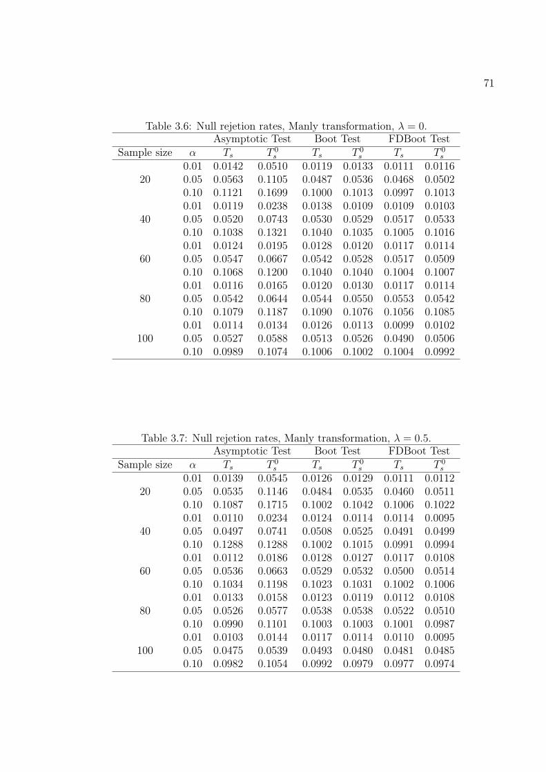
3.6 Null rejetion rates, Manly transformation, λ = 0. 71
3.7 Null rejetion rates, Manly transformation, λ = 0.5. 71
3.8 Null rejetion rates, Manly transformation, λ = 1. 72
3.9 Null rejetion rates, Manly transformation, λ = 1.5. 72
3.10 Null rejetion rates, Manly transformation, λ = 2. 73
3.11 Power of tests, Box-Cox transformation, T = 40 and λ0 = 1. 74
Page 12
3.12 Power of tests, Manly transformation, T = 40 and λ0 = 1. 74
4.1 Biases, variances, MSEs of the estimators of λ (Box-Cox transformation
parameter) when λ0 = −1 (Case 1). 88
4.2 Biases, variances, MSEs of the estimators of λ (Box-Cox transformation
parameter) when λ0 = −0.5 (Case 1). 88
4.3 Biases, variances, MSEs of the estimators of λ (Box-Cox transformation
parameter) when λ0 = 0 (Case 1). 89
4.4 Biases, variances, MSEs of the estimators of λ (Box-Cox transformation
parameter) when λ0 = 0.5 (Case 1). 89
4.5 Biases, variances, MSEs of the estimators of λ (Box-Cox transformation
parameter) when λ0 = 1 (Case 1). 90
4.6 Biases, variances, MSEs of the estimators of λ (Manly transformation pa-
rameter) when λ0 = 0 (Case 1). 90
4.7 Biases, variances, MSEs of the estimators of λ (Manly transformation pa-
rameter) when λ0 = 0.5 (Case 1). 91
4.8 Biases, variances, MSEs of the estimators of λ (Manly transformation pa-
rameter) when λ0 = 1 (Case 1). 91
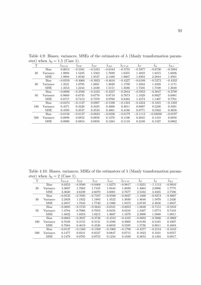
4.9 Biases, variances, MSEs of the estimators of λ (Manly transformation pa-
rameter) when λ0 = 1.5 (Case 1). 92
4.10 Biases, variances, MSEs of the estimators of λ (Manly transformation pa-
rameter) when λ0 = 2 (Case 1). 92
4.11 Biases, variances, MSEs of the estimators of λ (Box-Cox transformation
parameter) when λ0 = −1 (Case 2). 94
4.12 Biases, variances, MSEs of the estimators of λ (Box-Cox transformation
parameter) when λ0 = −0.5 (Case 2). 94
4.13 Biases, variances, MSEs of the estimators of λ (Box-Cox transformation
parameter) when λ0 = 0 (Case 2). 95
Page 13
4.14 Biases, variances, MSEs of the estimators of λ (Box-Cox transformation
parameter) when λ0 = 0.5 (Case 2). 95
4.15 Biases, variances, MSEs of the estimators of λ (Box-Cox transformation
parameter) when λ0 = 1 (Case 2). 96
4.16 Biases, variances, MSEs of the estimators of λ (Manly transformation pa-
rameter) when λ0 = 0 (Case 2). 96
4.17 Biases, variances, MSEs of the estimators of λ (Manly transformation pa-
rameter) when λ0 = 0.5 (Case 2). 97
4.18 Biases, variances, MSEs of the estimators of λ (Manly transformation pa-
rameter) when λ0 = 1 (Case 2). 97
4.19 Biases, variances, MSEs of the estimators of λ (Manly transformation pa-
rameter) when λ0 = 1.5 (Case 2). 98
4.20 Biases, variances, MSEs of the estimators of λ (Manly transformation pa-
rameter) when λ0 = 2 (Case 2). 98
4.21 Biases, variances, MSEs of the estimators of λ (Box-Cox transformation
parameter) when λ0 = −1 (Case 3). 100
4.22 Biases, variances, MSEs of the estimators of λ (Box-Cox transformation
parameter) when λ0 = −0.5 (Case 3). 100
4.23 Biases, variances, MSEs of the estimators of λ (Box-Cox transformation
parameter) when λ0 = 0 (Case 3). 101
4.24 Biases, variances, MSEs of the estimators of λ (Box-Cox transformation
parameter) when λ0 = 0.5 (Case 3). 101
4.25 Biases, variances, MSEs of the estimators of λ (Box-Cox transformation
parameter) when λ0 = 1 (Case 3). 102
4.26 Biases, variances, MSEs of the estimators of λ (Manly transformation pa-
rameter) when λ0 = 0 (Case 3). 102
4.27 Biases, variances, MSEs of the estimators of λ (Manly transformation pa-
rameter) when λ0 = 0.5 (Case 3). 103
Page 14
4.28 Biases, variances, MSEs of the estimators of λ (Manly transformation pa-
rameter) when λ0 = 1 (Case 3). 103
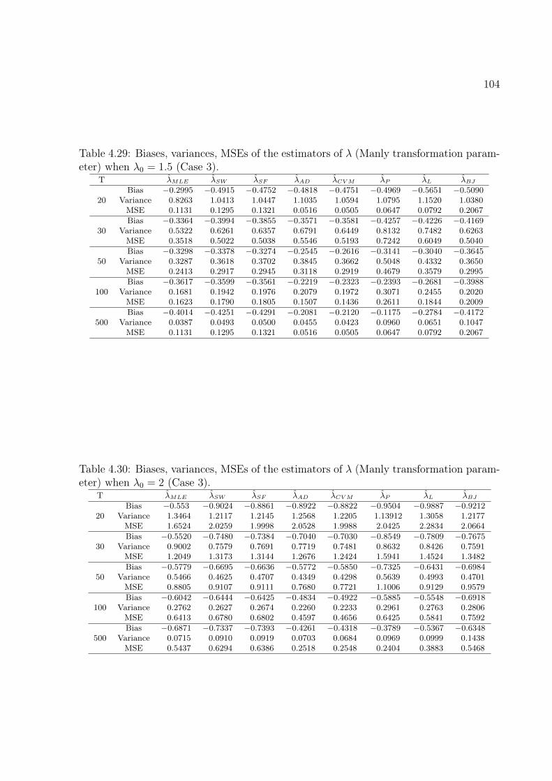
4.29 Biases, variances, MSEs of the estimators of λ (Manly transformation pa-
rameter) when λ0 = 1.5 (Case 3). 104
4.30 Biases, variances, MSEs of the estimators of λ (Manly transformation pa-
rameter) when λ0 = 2 (Case 3). 104
4.31 Descriptive statistics of breaking distance and speed. 105
4.32 Parameter estimates, p-values and R2. 107
4.33 Tests p-values. 109
Page 15
Contents
1 Introduction 17
2 Score tests for response variable transformation in the linear regression
model 20
2.1 Resumo 20
2.2 Abstract 21
2.3 Introduction 21
2.4 The linear regression model 22
2.5 Parameter estimation 24
2.5.1 Ordinary least squares 24
2.5.2 Maximum likelihood estimator 26
2.6 Transformations 27
2.7 Transformation data tests 31
2.7.1 Approximate tests 31
2.7.2 Score test for λ 36
2.8 Bootstrap hypothesis testing 42
2.9 Simulation results 43
2.9.1 Tests sizes 44
2.9.2 Tests powers 50
2.10 Application 51
2.11 Conclusions 58
3 Fast double bootstrap 59
3.1 Resumo 59
3.2 Abstract 60
3.3 Introduction 60
3.4 Score test for λ 61
Page 16
3.5 Double bootstrap and fast double bootstrap tests 62
3.6 Simulation results 66
3.6.1 Tests sizes 67
3.6.2 Tests powers 68
3.7 Conclusions 74
4 Estimators of the transformation parameter via normality tests 76
4.1 Resumo 76
4.2 Abstract 77
4.3 Introduction 77
4.4 Transformations 78
4.5 Some well-known normality tests 79
4.5.1 Shapiro-Wilk test 79
4.5.2 Shapiro-Francia test 80
4.5.3 Kolmogorov-Smirnov test 81
4.5.4 Lilliefors test 82
4.5.5 Anderson-Darling test 82
4.5.6 Cramér-Von Mises test 83
4.5.7 Pearson chi-square test 83
4.5.8 Bera-Jarque test 83
4.6 Simulation setup 84
4.7 Simulation results 86
4.7.1 Case 1: Estimation for a continuous variable 87
4.7.2 Case 2: Estimation for the response of linear model with normality
assumption 93
4.7.3 Case 3: Estimation for the response of linear model without nor-
mality assumption 99
4.8 Application 105
4.9 Conclusions 113
Page 17
5 Final Considerations 114
References 116
Page 18
CHAPTER 1
Introduction
Regression analysis is of paramount importance in many areas, such as engineering,
physics, economics, chemistry, medicine, among others. Even though the classic linear
regression model is commonly used in empirical analysis, its assumptions are not always
valid. For instance, the normality and homoskedasticy assumptions are oftentimes vio-
lated.
An alternative is to use transformations on the response variable. According to Box
and Tidwell (1962), variable transformation can be applied without harming the norma-
lity and homoskedasticy of the model’s errors. The most popular transformation is the
Box-Cox transformation (Box and Cox, 1964), because it covers the logarithmic transfor-
mation and also the no transformation case. The Box-Cox transformation, however, has
a limitation: it requires the variable only assumes positive values. There are transfor-
mations that can be used when the variable assumes negative values, such as the Manly
(1976) and Bickel and Doksum (1981) transformations.
17
Page 19
18In this PhD dissertation we consider data transformations. It consists of four chap-
ters. In Chapter 2 we develop two score tests for the Box-Cox and Manly transformations
(Ts and T 0s ). Monte Carlo simulations are performed to evaluate the proposed tests finite
sample behavior. We also consider bootstrap versions of the tests. The numerical evidence
shows that Ts outperforms T 0s test, both in terms of size and power. Additionally, the
bootstrap versions of the tests outperform their asymptotic counterparts. Furthermore,
as the sample size increases the performances of the tests become similar.
In Chapter 3 we seek to improve the accuracy of the score tests developed in Chap-
ter 2 using the fast double bootstrap. We perform Monte Carlo simulations to evaluate
the finite sample performances of the tests based on the fast double bootstrap. The
results show that the fast double bootstrap tests are superior to the standard bootstrap
tests, since it leads to tests with superior null and non null both is terms of size and power.
In Chapter 4 we consider estimators for the parameters that index the Box-Cox and
Manly transformations that are based on normality tests. We perform several Monte Carlo
simulations to evaluate the estimators finite sample performances. The finite sample per-
formances of the proposed estimators are compared to that of the maximum likelihood
estimator in three cases. First, to transform a non-normal variable, second to transform
the response variable of a linear regression model when the normality assumption is not
violated and third to transform the response variable of the linear regression model when
the normality assumption is violated.
This PhD dissertation was written using LATEX, which is a typesetting system that
includes features designed for the production of technical and scientific documentation
(Lamport, 1986). The numeric evaluations in Chapters 2 and 3 were carried out u-
sing the Ox matrix programming language. Ox is freely available for academic use at
http://www.doornik.com. Ox is an object-oriented matrix programming language with
Page 20
19a mathematical and statistical functions library and maintained by Jurgen Doornik. The
numeric evaluations in Chapter 4 and the applications were performed using the software
R version 3.3.0 for the Windows operational system (R Development Core Team, 2016).
R is freely available at http://www.R-project.org.
Page 21
CHAPTER 2
Score tests for response variable transformation in the linear
regression model
2.1 Resumo
O modelo de regressão linear é frequentemente usado em diferentes áreas do conheci-
mento. Muitas vezes, no entanto, alguns pressupostos são violados. Uma possível solução
é transformar a variável resposta. Yang and Abeysinghe (2003) propuseram testes escore
para estimar o parâmetro que indexa a transformação de Box-Cox para transformar as
variáveis do modelo de regressão linear. Tal transformação, no entanto, não pode ser
usada quando a variável assume valores negativos. Neste capítulo, propomos dois testes
score que podem ser usados para estimar os parâmetros das transformações de Box-Cox
e Manly no caso da transformação da variável resposta do modelo de regressão linear.
Foram feitas simulações de Monte Carlo para tamanhos de amostra finitos. Inferências
baseadas no método bootstrap também foram consideradas. Uma aplicação empírica foi
proposta e discutida.
20
Page 22
21
Palavras-chave: Bootstrap; Monte-Carlo; Transformação de Box-Cox; Transformação
de Manly; Teste score.
2.2 Abstract
The linear regression model is frequently used in empirical applications in many di-
fferent fields. Oftentimes, however, some of the relevant assumptions are violated. A
possible solution is to transform the response variable. Yang and Abeysinghe (2003) pro-
posed score tests that can be used to determine the value of the parameter that indexes
the Box-Cox transformation to transform the variables of a linear model regression. Such
a transformation, however, cannot be used when the variable assumes negative values. In
this chapter, we propose two score tests to estimate the parameters of the Box-Cox and
Manly transformations when we transform the response of a linear regression model. We
report Monte Carlo simulation results on the tests finite sample behaviors. Bootstrap-
based testing inference is also considered. An empirical application is proposed and dis-
cussed.
keywords: Bootstrap; Box-Cox transformation; Manly transformation; Monte Carlo
simulation; Score test.
2.3 Introduction
Regression analysis is of extreme importance in many areas, such as engineering,
physics, economics, chemistry, medicine, among others. Although the classic linear regres-
sion model is commonly used in empirical analysis, its assumptions are not always valid.
For instance, the normality and homoskedasticy assumptions are oftentimes violated.
Page 23
22An alternative is to use transformations on the response variable. According to Box
and Tidwell (1962), variable transformation can be applied without harming the normal-
ity and homoskedasticy of the model’s errors. The most popular transformation is the
Box-Cox transformation (Box and Cox, 1964), because it covers the logarithmic transfor-
mation and also the no transformation case. The Box-Cox transformation, however, has
a limitation: it requires the variable to be transformed to only assume positive values.
There are transformations can be used when the variable assumes negative values, such
as the Manly (1976) and Bickel and Doksum (1981) transformations.
Estimation of the parameter that indexes the transformation is usually done by ma-
ximum likelihood. Yang and Abeysinghe (2003) proposed two score tests (Rao, 1948)
that can be used to determine the value of the Box-Cox transformation parameter when
it is simultaneously applied to the independent and response variables of the linear re-
gression model. In this chapter we present two score tests for the parameters that index
the Box-Cox and Manly transformations, to the response of classic linear regression model.
2.4 The linear regression model
Regression analysis is used to model the relationship between variables in almost all
areas of knowledge. The interest lies in studying the dependence of a variable of interest
(response, dependent variable) on a set of independent variables (regressor covariates).
The response variable can be continuous, discrete or a mixture of both. The proposed
model should take into account its nature.
Let y1, . . . , yT be independent random variables. The linear regression model is given
by
Page 24
23
yt = β1 + β2xt2 + β3xt3 + · · ·+ βpxtp + εt, t = 1, . . . , T, (2.1)
where yt is the tth response, xt2, . . . , xtp are the tth observation on p−1 (p < T ) regressors
which influence the mean response; µt = IE(yt), β1, . . . , βp are the unknown parameters
and εt is the tth error. The model can be written in matrix form as
y = Xβ + ε,
where y is a (T × 1) response vector, β is a (p× 1) vector of parameters, X is the (T × p)
(p < T ) matrix of regressors (rank (X) = p) and ε is a (T × 1) vector of random errors.
Some assumptions are commonly made:
[S0] The estimated model is the correct model;
[S1] IE(εt) = 0 ∀t;
[S2](homoskedasticity) var(εt) = IE(ε2t ) = σ2 (0 < σ2 <∞) ∀t;
[S3](non-autocorrelation) cov(εt, εs) = IE(εtεs) = 0 ∀t 6= s;
[S4] The only values c1, c2, . . . , cp such that c1 + c2xt2 + · · ·+ cpxtp = 0 ∀t are c1 = c2 =
· · · = ck = 0, i.e., the columns of X are linearly independent, that is, X has full rank:
rank(X) = p (< T );
[S5] (normality) εt ∼ Normal ∀t. This implies that yt ∼ Normal. This assumption is often
used for interval estimation and hypothesis testing inference.
The parameters can be interpreted in terms of the mean response, since
µt = β1 + β2xt2 + · · ·+ βpxtp, t = 1, 2, . . . , T.
For example, β1 is the mean of yt when all regressors equal zero. Additionally, βj (j =
2, . . . , p) measures the change in the mean response when xtj increases by one unit and
all other regressors remain fixed.
Page 25
24
2.5 Parameter estimation
2.5.1 Ordinary least squares
For the model
yt = β1 +
p∑j=2
βjxtj + εt, t = 1, . . . , T,
the sum of squared errors is given by
S ≡ S(β1, . . . , βp)> =
T∑t=1
ε2t =T∑t=1
(yt − β1 −
p∑j=2
βjxtj
)2
.
The ordinary least squares estimators of β1, . . . , βp are obtained by minimizing S with
respect to regression parameters. The first order conditions are
∂S
∂β1= −2
T∑i=1
(yt − β1 −
p∑j=2
βjxtj
)= 0
and
∂S
∂βj= −2
T∑i=1
(yt − β1 −
p∑j=2
βjxtj
)xtj = 0, j = 2, . . . , p.
We thus have the following system of normal equations:
Page 26
25
T β1 + β2
T∑t=1
xt2 + β3
T∑t=1
xj3 + · · ·+ βp
T∑t=1
xtp =T∑t=1
yt
β1
T∑t=1
xt2 + β2
T∑t=1
x2t2 + β3
T∑t=1
xt2xt3 + · · ·+ βp
T∑t=1
xt2xtp =T∑t=1
xt2yt
...
β1
T∑t=1
xtp + β2
T∑t=1
xtpxt2 + β3
T∑t=1
xtpxt3 + · · ·+ βp
T∑t=1
x2tp =T∑t=1
xtpyt,
where β1, . . . , βp are the ordinary least squares estimators of β1, . . . , βp. We can write the
above system of equations in matrix form as
−2X>y + 2X>Xβ = 0,
where β = (β1, . . . , βp)> is the vector of estimators of ordinary least squares of β.
The second order condition is satisfied since
∂S2
∂β∂β>= 2X>X
is positive definite.
Finally, the least squares estimator of the error variance is given by
σ2 =
∑Tt=1 ε
2t
T − p=
ε>ε
T − p,
where εt is the tth residual and ε = (ε1, . . . , εT )>, i.e., εt = yt − xt>β, where xt is the tth
line of X.
Page 27
26An important result is the Gauss-Markov Theorem which establishes the optimality
of β.
Theorem 2.5.1 (Gauss-Markov Theorem). In the linear regression model with Assump-
tions [S0], [S1], [S2], [S3] and [S4] ([S4] for X>X to be non-singular), we have that the
ordinary least squares estimator β is the best linear and unbiased estimator of β.
2.5.2 Maximum likelihood estimator
Using Assumption [S5] that yt is normally distributed and assumptions [S0], [S1], [S2]
and [S3] the vector of errors ε is distributed as N(0, σ2Id), where Id is the identity matrix
of order T . Since IE(y) = Xβ, y has distribution N ∼ (Xβ, σ2Id).
The likelihood function is given by
L(β, σ2|y,X) = (2πσ2)T/2exp{− 1
2σ2(y −Xβ)>(y −Xβ)
}and the log-likelihood function is
` = log(L(β, σ2|y,X)) = −T2log(2π)− T
2log(σ2)− 1
σ2(y −Xβ)>(y −Xβ).
The maximum likelihood estimators (MLE) of β and σ2 are, respectively,
βML = (X>X)−1X>y
and
σ2ML =
ε>ε
T.
Note that, under normality, the least squares estimator and the MLE of β coincide,
Page 28
27but the σ2
ML and σ2 not coincide. σ2ML is biased, while σ2 is unbiased. It is also notewor-
thy that the MLE of β and σ2 are independent. The same holds for the ordinary least
squares estimators under normality.
2.6 Transformations
Oftentimes some assumptions of the linear regression model are violated, for example,
when there is multicollinearity and as a consequence the Assumption [S4] is violated.
This problem occurs when rank(X) < p. We say that there is exact multicollinearity if
∃ c = (c1, . . . , cp)> 6= 0 such that
c1x1 + c2x2 + · · ·+ cpxp = 0, (2.2)
where xj is the jth column of X, j = 1, . . . , p.
There is near exact multicollinearity when Equation (2.2) holds approximately. Under
exact multicollinearity X>X becomes singular, so we cannot obtain the maximum like-
lihood estimator βMV uniquely. Additionally, it is impossible to estimate the individual
effects of regressors on the mean response, because we cannot vary a regressor and keep
other regressors constant. Under near exact multicollinearity, we can estimate such effects,
but the estimates are imprecise and have large variances, sinceX>X is close to singularity.
Other assumptions that are often violated are [S0] and [S5], linearity and normality,
respectively. In many cases, transformation of the response variable may be desirable
(Box and Cox, 1964).
The most well known data transformation is the Box-Cox transformation (Box and
Cox, 1964). It is given by
Page 29
28
yt(λ) =
yλt −1λ
, if λ 6= 0
log (yt) , if λ = 0.
Using the L’Hôpital’s rule, it is easy to show that log(yt) is the limit of (yλt − 1)/λ
when λ→ 0. In practice, λ usually assumes values between −2 and 2.
The popularity of this transformation is partially due to the fact that it includes as
special cases both the no transformation case (λ = 1) and the logarithmic (λ = 0) trans-
formation. Furthermore, it often reduces deviations from normality and homoskedasticity
and it is easy to use. Figure 2.1 contains plots of yt(λ) versus yt for different values of λ.
Notice that as the value of λ moves away from one the curvature of the transformation
increases (Davidson and MacKinnon, 1993).
Figure 2.1: Box-Cox transformation with λ = 2, 1.5, 1, 0.5, 0,−0.5,−1,−1.5 and − 2, lineof the highest to the lowest, respectively.
The main disadvantage of the Box-Cox transformation is that it can only be applied to
positive data. Another disadvantage is the fact that the transformed response is bounded
Page 30
29(except for λ = 0 and λ = 1). By applying the Box-Cox transformation to the response
variable in Equation (2.1) we have
yt(λ) = β1 + β2xt2 + · · ·+ βpxtp + εt, t = 1, . . . , T. (2.3)
Thus, the left hand side of Figure 2.1 is bounded whereas the right hand side is un-
bounded. When λ > 0, yt(λ) ≥ −1/λ and when λ < 0, yt(λ) ≤ −1/λ.
Another disadvantage of the Box-Cox transformation is that the inferences made after
the response variable are conditional on the value of λ selected (estimated) and neglect
the uncertainly involved in the estimation of λ.
Finally, an additional negative point is that the model parameters (β1, β2, . . . , βp)>
become interpretable in terms of the mean of y(λ) and not in terms of the mean of
y, which is the variable of interest. It follows from Equation (2.3) that β2 measures
the variation in IE(y(λ)) when x2 increases by one unit and all other covariates remain
constant. It follows from Jensen’s inequality that the parameters of the regression of y(λ)
on x2, . . . , xp cannot be interpreted in terms of the mean of y:
Jensen’s inequality: Let Z be a random variable such that IE(Z) exists. If g is a
convex function, then
IE(g(Z)) ≥ g(IE(Z))
and if g is concave, then
IE(g(Z)) ≤ g(IE(Z)),
equality only holding under linearity.
An useful alternative to the Box-Cox transformation that can be used with negative
data is the Manly transformation (Manly, 1976). This transformation is quite effective
in transforming unimodal distributions into almost symmetrical ones (Manly, 1976). It is
Page 31
30given by
yt(λ) =
eλyt−1λ
, if λ 6= 0
yt , if λ = 0.
Similarly to the Box-Cox transformation, the left hand side of the regression equa-
tion that uses yt(λ) is bounded whereas the right hand side is unbounded. When λ is
positive, y(λ) assumes values between −1/λ and +∞; when λ is negative, y(λ) assumes
values between −∞ and −1/λ. Draper and Cox (1969) noted that if λ is chosen so as
to maximize the likelihood function constructed assuming normality, the transformation
tends to minimize deviations from such an assumption. Figure 2.2 contains plots of yt(λ)
against yt for different values of λ. Note that as the value of λ moves away from zero the
curvature of transformation increases. Additionally, for λ < 0 the transformation is not
strictly increasing when y > 0.
Figure 2.2: Manly transformations with λ = 2, 1.5, 1, 0.5, 0,−0.5,−1,−1.5 and − 2, lineof the highest to the lowest, respectively.
As with Box-Cox transformation, a disadvantage of the Manly transformation is that
Page 32
31the inferences made after the response is transformed are conditional on the value of λ se-
lected and neglect the uncertainty involved in the estimation of λ. Another disadvantage
is that the two transformations share lies in the fact that when using the transformed
variable in the regression model, the parameters (β1, β2, . . . , βp)> become interpretable in
terms of the mean of y(λ) and not of the mean of y, which is the variable of interest.
2.7 Transformation data tests
Oftentimes one is faced with the need to transform data. The transformations used
are typically determined by a scale parameter. The estimation of such a parameter is
commonly made by maximum likelihood. Additionally, one has the option of testing
whether parameter value is equal to a given value.
2.7.1 Approximate tests
Hypothesis testing inference is usually made using likelihood-based tests. Let θ ⊆ Θ
where Θ ⊂ IRp and let be y1, . . . , yT independent and identically distributed random
variables. The likelihood function is given by
L(θ) =T∏t=1
f(yt; θ),
where yt is the tth realization of the random variable y which is characterized by the
probability density function f(y; θ). We usually obtain maximum likelihood estimates by
maximizing the log-likelihood `(θ) = log(L(θ)).
Consider the following partition of θ = (θ>1 , θ>2 )>, where θ1 is a (q×1) interest param-
eter vector and θ2 is a ((p− q)× 1) nuisance parameter vector. Suppose we want to test
H0 : θ1 = θ(0)1 against H1 : θ1 6= θ
(0)1 , where θ(0)1 is a given vector of dimension q × 1. Let
θ = (θ>1 , θ>2 )> denotes the unrestricted MLE of θ and let θ = (θ
(0)1
>, θ>2 )> be the restricted
Page 33
32MLE of θ, where θ2 is obtained by maximizing the log-likelihood function by imposing
that θ1 = θ(0)1 .
The likelihood ratio test is the most used likelihood-based test and is based on the
difference between the values of the log-likelihood function evaluated at θ and at θ. The
test statistic is
RV = 2(`(θ)− `(θ)
).
A special case occurs when there is no nuisance parameter in θ, i.e., we test H0 : θ =
θ(0) versus H1 : θ 6= θ(0), where θ(0) is a (p × 1) vector. The likelihood ratio statistic
becomes
RV = 2(`(θ)− `(θ(0))
).
An even more particular case occurs when θ is scalar. Here, we test H0 : θ = θ0 versus
H1 : θ 6= θ0, where θ0 is a given scalar. The likelihood ratio test statistic is given by
RV = 2(`(θ)− `(θ0)
).
In the general case where we test q restrictions and under H0,
RVD−→ χ2
q,
where D−→ denotes convergence in distribution. We reject H0 if RV > χ2(1−α),q, where
χ2(1−α),q is the (1− α) upper quantile of the χ2
q distribution.
Figure 2.3 graphically displays the likelihood function when θ is scalar. Note that for
a given distance θ − θ0, the larger the curvature of the function the larger the distance
between logL(θ) and logL(θ0), i.e., the larger (1/2)RV .
Page 34
33
Figure 2.3: Log-likelihood function.
Another test that is commonly used to test hypothesis on θ is the score test or the
Lagrange multiplier test (Rao, 1948). Let S(θ) be the score vector, i.e.,
S(θ) =∂`(θ)
∂θ.
Fisher’s information matrix is given by
I(θ) = IE
(∂`(θ)
∂θ
∂`(θ)
∂θ>
).
Under certain regularity conditions (Cordeiro and Cribari-Neto, 2014), we have
I(θ) = IE
(−∂
2`(θ)
∂θ∂θ>
).
According to partition of θ, we can partition Fisher’s information as follows:
I(θ) =
Kθ1θ1 Kθ1θ2
Kθ2θ1 Kθ2θ2
,where Kθiθj = IE
(− ∂2`(θ)∂θi∂θj
), for i, j = 1, 2. The inverse of Fisher’s information matrix is
denoted as
I(θ)−1 =
Kθ1θ1 Kθ1θ2
Kθ2θ1 Kθ2θ2
.
Page 35
34Here, Kθ1θ1 is the (q × q) matrix formed by the first q lines and the first q columns of
I(θ)−1. Using the fact that I(θ) = var(S(θ)) and the Central Limit Theorem, we have
that when the sample size is large, θ ∼ N(θ, I(θ)−1), approximately.
Consider the case where we test H0 : θ1 = θ(0)1 versus H1 : θ1 6= θ
(0)1 and S(θ1) contains
the first q score vector elements. The score statistic can be written as
Sr = S(θ1)>Kθ1θ1S(θ1),
where tildes indicate that quantities are evaluated at θ. When there is no nuisance
parameter, i.e., when we test H0 : θ = θ(0) versus H1 : θ 6= θ(0), the score statistic became
Sr = S(θ(0))>I(θ(0))−1S(θ(0)). (2.4)
When θ is scalar and we test H0 : θ = θ0 versus H1 : θ 6= θ0, the score statistic reduces to
Sr =S(θ0)
2
I(θ0).
In the general case where we test q restrictions, we have that, under H0,
SrD−→ χ2
q.
We reject H0 if Sr > χ2(1−α),q.
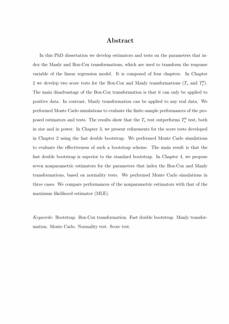
Figure 2.4 graphically displays the score function when θ is scalar. Note that the score
test statistic is based on the curvature of the log-likelihood function evaluated at θ0.
The Wald statistic is which is based on the difference between θ1 and θ(0)1 (Wald, 1943).
In the general case where we test H0 : θ1 = θ(0)1 versus H1 : θ1 6= θ
(0)1 , the Wald statistic
is given by
Page 36
35
Figure 2.4: Log-likelihood function and the score statistic.
W = (θ1 − θ(0)1 )>Kθ1θ1(θ1 − θ(0)1 ),
where Kθ1θ1 is the matrix formed by the first q lines and the first q columns of Fisher’s
information matrix evaluated at θ. When there is no nuisance parameter, i.e., when we
test H0 : θ = θ(0) versus H1 : θ 6= θ(0), the Wald statistic is given by
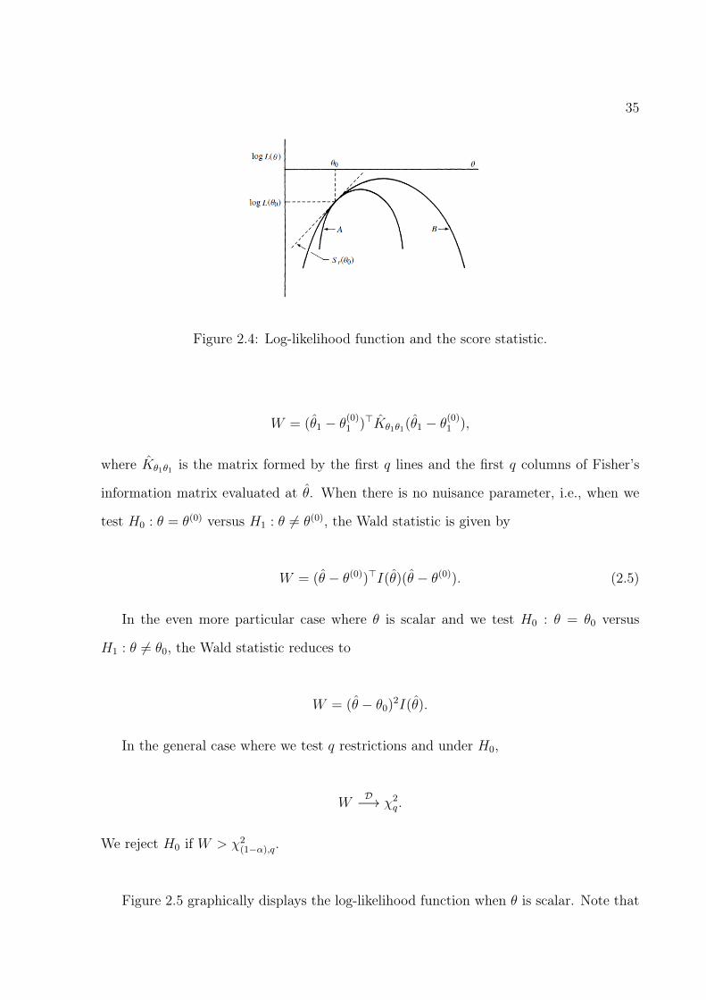
W = (θ − θ(0))>I(θ)(θ − θ(0)). (2.5)
In the even more particular case where θ is scalar and we test H0 : θ = θ0 versus
H1 : θ 6= θ0, the Wald statistic reduces to
W = (θ − θ0)2I(θ).
In the general case where we test q restrictions and under H0,
WD−→ χ2
q.
We reject H0 if W > χ2(1−α),q.
Figure 2.5 graphically displays the log-likelihood function when θ is scalar. Note that
Page 37
36the Wald statistic is based on the horizontal difference between θ and θ0. The score test is
usually the most convenient test to use, since it only requires estimation of the restricted
model.
Figure 2.5: Log-likelihood function and the Wald statistic.
Terrell (2002) combined the score statistic and the Wald statistic in a single statistic.
It was named the gradient statistic. Acording to Lemonte (2016), consider the case when
we test H0 : θ = θ(0) versus H1 : θ 6= θ(0) and consider Equations (2.4) and (2.5). Choose
any square root A of I(θ(0)), that is, A>A = I(θ(0)). So (A−1)>S(θ(0)) and A(θ− θ(0)) are
asymptotically distributed as N(0, I(θ(0))) and (A−1)>S(θ(0))− A(θ − θ(0)) P−→ 0. Under
H0,
STD−→ χ2
p.
2.7.2 Score test for λ
In regression models where the response is transformed by an unknown parameter λ,
we have to estimate this parameter. Consider the model described in Equation (2.1). The
Box-Cox transformation of the response variable is given by
Page 38
37
yt(λ) =
yλt −1λ
, if λ 6= 0
log(yt) , if λ = 0.
Using this transformation we arrive at the following model:
yt(λ) = β1 +
p∑j=2
βjxtj + εt, t = 1, . . . , T ,
where yt(λ) is the transformed response variable. Assuming normality and the indepen-
dence of errors, the log-likelihood function is
`(β, σ2, λ) ∝ −T2log(σ2)− 1
2σ2
T∑t=1
{yt(λ)−
p∑j=0
βjxtj
}2
+ log J(λ),
where σ2 is the variance of the error and J(λ) is the Jacobian of the Box-Cox transfor-
mation, which is given by
J(λ) =T∏t=1
∂yt(λ)
∂yt=
T∏t=1
y(λ−1)t .
For a given λ, the maximum likelihood estimators of β and σ2 are, respectively,
β(λ) = (X>X)−1X>y(λ)
and
σ2(λ) =‖My(λ)‖2
T,
where ‖·‖ is the Euclidian norm and M = IdT −X(X>X)−1X>.
The profile log-likelihood function for λ is
`p(λ) = `[β(λ), σ2(λ), λ] ∝ −T2log σ2(λ) + log J(λ). (2.6)
Page 39
38Therefore, the score function for λ is
Sp(λ) =∂`p(λ)
∂λ= − 1
σ2e>[λ, β(λ)]e[λ, β(λ)] +
T∑t=1
log yt,
where e = e(λ, β(λ)) = y(λ) − Xβ(λ) and e = ∂e(λ, β(λ))/∂λ. Additionally, y(λ) =
∂y(λ)/∂λ is given by
yt(λ) =
1λ[1 + λyt(λ)]logyt − 1
λyt(λ) , if λ 6= 0
12(logyt)2 , if λ = 0
.
We obtain the MLE of λ by maximizing `p(λ) with respect to λ.
Suppose we wish to test H0 : λ = λ0 versus H1 : λ 6= λ0. The profile score test statistic
is
Ts(λ0) =Sp(λ0)
$[β(λ0), σ2(λ0), λ0],
where $[β(λ), σ2(λ), λ] = Iλλ − IλψI−1ψψIψλ is the asymptotic variance S(λ) and ψ =
(β>, σ2)>. For simplicity, in what follows we shall refer to the profile score test simply as
the score test statistic.
The I-quantities are the elements of the expected information matrix. They can be
expressed as
Iββ =1
σ2X>X,
Iσ2σ2 =T
2σ4,
Iλλ =1
σ2IE[e(λ, β)>e(λ, β) + e(β, λ)>e(λ, β)],
Page 40
39
Iβλ = − 1
σ2[X>IE[e(λ, β)]],
Iβσ2 = 0,
Iσ2λ = − 1
2σ4IE[e(λ, β)>e(λ, β)],
where e = ∂2e(λ, β)/∂λ2.
Additionally, y(λ) is given by
yt(λ) =
yt(λ)[log(yt)− 1
λ
]− 1
λ2[log(yt)− yt(λ)] , if λ 6= 0
13[log(yt)]
3 , if λ = 0.
Since it is usually not trivial to obtain the elements of the expected information matrix,
it is customary to replace them by the corresponding observed quantities. The elements
of the observed information matrix, the J-quantities, are given by
Jββ = − ∂2`
∂β∂β>=
1
σ2X>X,
Jσ2σ2 = − ∂2`
∂(σ2)2= − T
2σ4+
1
σ6e(λ, β)>e(λ, β),
Jλλ = −1
2
∂2`
∂(λ2)= − 1
σ2[e(λ, β)>e(λ, β) + e(λ, β)>e(λ, β)],
Jβσ2 = − ∂2`
∂β∂σ2=
1
σ4X>e(λ, β),
Jβλ = − ∂2`
∂β∂λ= − 1
σ2X>e(λ, β),
Page 41
40
Jσ2λ = − ∂2`
∂σ2∂λ= − 1
σ4e(λ, β)>e(λ, β).
Yang and Abeysinghe (2002) obtained an approximate formula for the asymptotic
variance of the MLE λ. Using the result that var[S(λ)] = 1/var(λ), in large sample sizes,
the asymptotic variance of S(λ) can be approximated by
$[β, σ2, λ] ≈ 1
σ2‖Mδ‖2 +
1
λ2
[2‖φ− φ‖2 − 4(φ− φ)>(θ2 − θ2) +
3
2‖θ‖2
], (2.7)
where µ(λ) = Xβ(λ), φ = log(1 + λµ(λ)), θ = λσ1+λµ(λ)
and δ = 1λ2(1+λµ(λ))#φ
+ (σ/2λ)θ.
Here, a denotes the average of the elements of the vector a and a#b denotes the direct
product between vectors a and b (both of the same dimension).
When λ = 0, the asymptotic variance of Sp(λ) can be approximated by
$[β, σ2, 0] ≈ 1
σ2‖Mδ‖2 + 2 ‖µ(0)− µ(0)‖2 +
3
2Tσ2, (2.8)
where δ = 1/2[µ(0)2 + σ2].
We can alternatively use the observed information matrix. Here, we replace Iλλ −
IλψI−1ψψIψλ by Jλλ − JλψJ−1ψψJψλ. In this case, note that Jβσ2 = 0. Thus, the asymptotic
variance Sp(λ) can be approximated by
κ[β, σ2, λ] = Jλλ − Jσ2βJ−1ββ Jβσ2 − Jλσ2J−1σ2σ2Jσ2λ. (2.9)
The score statistic is given by
T 0s (λ0) =
Sp(λ0)
κ[β(λ0), σ2(λ0), λ0].
The variance of Sp(λ) is obtained from the observed information matrix and cannot be
guaranteed to be positive. We then have two score tests for the parameter that indexes
Page 42
41the Box-Cox transformation.
We shall now develop two score tests for the parameter that indexes the Manly trans-
formation. Consider the model given in Equation (2.1). By applying the Manly transfor-
mation to the variable response we obtain
yt(λ) =
eytλ−1λ
, if λ 6= 0
yt , if λ = 0.
Assuming normality and independence, it follows that
`(β, σ2, λ) ∝ −T2log(σ2)− 1
2σ2
T∑t=1
{yt(λ)−
p∑j=0
βjxtj
}2
+ log J(λ),
where σ2 is the error variance and J(λ) is the Jacobian of the Manly transformation:
J(λ) =T∏t=1
eλyt .
The score function for λ is
Sp(λ) =∂`p(λ)
∂λ= − 1
σ2e>(λ, β(λ))e(λ, β(λ)) +
T∑t=1
yt,
where `p(λ) is the profile log-likelihood function given in Equation (2.6). The first and
second order derivatives of the transformed response with respect to λ are
yt(λ) =
eλyt (λyt−1)+1
λ2, if λ 6= 0
y2t2
, if λ = 0
and
yt(λ) =
eλyt (λ2y2t−2λyt+2)−2
λ3, if λ 6= 0
y3t3
, if λ = 0.
Page 43
42We can then derive Ts(λ0) and T 0
s (λ0) using the Manly transformation, which allows
yt to assume any real value. Our interest lies in testing H0 : λ = λ0 versus H1 : λ 6= λ0.
We obtain the following test statistics, based on expected and observed information,
respectively:
Ts(λ0) =Sp(λ0)
$[β(λ0), σ2(λ0), λ0]
and
T 0s (λ0) =
Sp(λ0)
κ[β(λ0), σ2(λ0), λ0],
where the asymptotic variance $[β(λ), σ2(λ), λ] is given in Equations (2.7) and (2.8),
when λ0 6= 0 and λ0 = 0, respectively, its approximation obtained using J-quantities
being κ[β(λ0), σ2(λ0), λ0], as defined in Equation (2.9).
2.8 Bootstrap hypothesis testing
Our interest lies in testing H0 : λ = λ0 versus H1 : λ 6= λ0. The null distribution of the
score statistic converges to χ21 when T →∞. We use approximate critical values obtained
from the χ21 distribution when carrying out the test. An alternative approach is to use
bootstrap resampling to obtain estimated critical values. The general idea behind the
bootstrap method is to take the initial sample as if it is the population and then generate
B artificial samples from the initial sample (Efron, 1979). Bootstrap data resampling can
be performed parametrically or non-parametrically. The parametric bootstrap is used
when one is willing to assume a distribution for y. The non-parametric bootstrap is used
no distributional assumptions are to be made. We shall consider the parametric bootstrap
because we need to impose the null hypothesis when creating the pseudo-samples. When
performing bootstrap resamping we impose the null hypothesis. The bootstrap test is
performed as follows (we use the Ts statistic as an example):
Page 44
43• Consider a set of observations on the response y and on the covariates x2, . . . , xp;
• Transform y, than obtain y(λ0);
• Regress y(λ0) on X, obtain the model residuals, β(λ0) and σ2(λ0) and compute
Ts(λ0);
• Generate B artificial samples as follows: y∗t (λ0) = xt>β(λ0) + σ(λ0)ε
∗t , where ε∗t
iid∼
N(0, 1);
• For each artificial sample regress y∗t (λ0) on X, obtain β∗(λ0) and σ2∗(λ0) and com-
pute T ∗s (λ0);
• Obtain the level α bootstrap the critical value (BCV(1−α)) as the (1 − α) quantile
of T ∗s1(λ0), . . . , T ∗sB(λ0);
• Reject H0 if Ts(λ0) > BCV(1−α).
2.9 Simulation results
The finite sample performances of the proposed score tests shall now be evaluated using
Monte Carlo simulations. We consider two data transformations: Box-Cox and Manly.
Our goal lies in testing H0 : λ = λ0 versus H1 : λ 6= λ0, where λ is the parameter that
indexes the transformation. The results are based on 10, 000 Monte Carlo replications
with sample sizes T = 20, 40, 60, 80 and 100. The number of bootstrap replications is 500.
We consider the model
yt = β1 + β2xt2 + εt, t = 1, . . . , T,
where yt is the tth response, xt2 is the tth observation on the regressor, β1 and β2 are
the unknown parameters and εt is the tth error. The values of the single regressor are
randomly generated from the U(1, 6) distribution. The covariate values are kept constant
throughout the simulation. In the Monte Carlo scheme, the errors are generated from
Page 45
44the N(0, 1) distribution. For this we use the pseudo-random numbers generator develop
by Marsaglia (1997). The values of λ0 used are λ0 = 0, 0.5, 1, 1.5 and 2 for the Manly
transformation and λ0 = −1,−0.5, 0, 0.5 and 1 for the Box-Cox transformation. When
λ0 is negative, the true value of β is β = (−8.0,−1.25)>, and when λ0 is non negative we
used β = (8.0, 1.25)>. All simulations were performed using the Ox matrix programming
language (Doornik and Ooms (2006)).
2.9.1 Tests sizes
For each sample size we compute the null rejection rates of the tests of H0 : λ = λ0
versus H1 : λ 6= λ0 at the 1%, 5% and 10% nominal levels using both approximate χ21
critical values and bootstrap critical values. Data generation is performed using λ = λ0.
Tables 2.1 through 2.5 contain the null rejection rates of the score tests on the Box-
Cox transformation parameter with λ = −1,−0.5, 0, 0.5 and 1, respectively. Tables 2.6
through 2.10 contain the null rejection rates of the tests on the Manly transformation
parameter with λ = 0, 0.5, 1, 1.5 and 2, respectively. The results show that, for both
transformations, when sample size increases, the null rejection rates converge to the cor-
responding nominal levels. For example, in Table 2.1, the null rejection rate when T = 20
is 0.0370 and when T = 100 the rate is 0.0487, at the 5% nominal level (test based on Ts,
asymptotic critical values).
It is noteworthy that the Ts test tends to be conservative whereas the T 0s test tends
to be liberal. For example, in Table 2.8, their null rejection rates for T = 60 and at the
10% nominal level are, respectively, 0.0949 and 0.1061. Size distortions became smaller
when the tests are based on bootstrap critical values. For example, in Table 2.1, the
Ts null rejection rates for T = 100 and at the 10% nominal level of the asymptotic and
bootstrap tests are, respectively, 0.0945 and 0.0993. The only case when asymptotic tests
Page 46
45outperform bootstrap tests is the T 0
s test on the Box-Cox transformation parameter when
λ < 0 in large samples. For example, in Table 2.2, the T 0s null rejection rates for T = 100
and at the 10% nominal level of the asymptotic and bootstrap tests are, respectively,
0.1004 and 0.0972. In general, the Ts test slightly outperforms the T 0s test.
Table 2.1: Null rejection rates, Box-Cox transformation, λ = −1.Ts statistic T 0
s statisticSample size α Asymptotic Bootstrap Asymptotic Bootstrap
0.01 0.0074 0.0108 0.0189 0.010820 0.05 0.0370 0.0497 0.0619 0.0480
0.10 0.0793 0.0971 0.1148 0.09940.01 0.0087 0.0110 0.0126 0.0111
40 0.05 0.0455 0.0515 0.0566 0.04830.10 0.0896 0.0989 0.1076 0.09830.01 0.0110 0.0125 0.0117 0.0126
60 0.05 0.0467 0.0511 0.0533 0.05240.10 0.0935 0.1022 0.1026 0.10280.01 0.0086 0.0109 0.0103 0.0110
80 0.05 0.0467 0.0514 0.0500 0.04950.10 0.0944 0.1029 0.1023 0.10000.01 0.0090 0.0106 0.0094 0.0107
100 0.05 0.0487 0.0509 0.0508 0.05040.10 0.0945 0.0993 0.1004 0.0977
Page 47
46
Table 2.2: Null rejection rates, Box-Cox transformation, λ = −0.5.Ts statistic T 0
s statisticSample size α Asymptotic Bootstrap Asymptotic Bootstrap
0.01 0.0070 0.0106 0.0189 0.010620 0.05 0.0370 0.0492 0.0623 0.0476
0.10 0.0793 0.0969 0.1151 0.09900.01 0.0087 0.0110 0.0125 0.0111
40 0.05 0.0455 0.0514 0.0563 0.04830.10 0.0902 0.0983 0.1074 0.09810.01 0.0109 0.0122 0.0118 0.0122
60 0.05 0.0470 0.0514 0.0536 0.05210.10 0.0941 0.1023 0.1024 0.10260.01 0.0087 0.0110 0.0101 0.0111
80 0.05 0.0467 0.0512 0.0502 0.04950.10 0.0943 0.1029 0.1020 0.10010.01 0.0090 0.0104 0.0095 0.0105
100 0.05 0.0487 0.0510 0.0506 0.05030.10 0.0941 0.0996 0.1004 0.0972
Table 2.3: Null rejection rates, Box-Cox transformation, λ = 0.Ts statistic T 0
s statisticSample size α Asymptotic Bootstrap Asymptotic Bootstrap
0.01 0.0077 0.0112 0.0189 0.011220 0.05 0.0375 0.0491 0.0628 0.0477
0.10 0.0821 0.0974 0.1131 0.09720.01 0.0078 0.0104 0.0123 0.0105
40 0.05 0.0461 0.0494 0.0573 0.05050.10 0.0902 0.0981 0.1080 0.09730.01 0.0099 0.0125 0.0110 0.0124
60 0.05 0.0473 0.0518 0.0541 0.05240.10 0.0956 0.1032 0.1026 0.10210.01 0.0086 0.0110 0.0106 0.0111
80 0.05 0.0483 0.0512 0.0514 0.04950.10 0.0957 0.1029 0.1032 0.10010.01 0.0090 0.0104 0.0095 0.0105
100 0.05 0.0487 0.0510 0.0506 0.05030.10 0.0941 0.0996 0.1004 0.0972
Page 48
47
Table 2.4: Null rejection rates, Box-Cox transformation, λ = 0.5.Ts statistic T 0
s statisticSample size α Asymptotic Bootstrap Asymptotic Bootstrap
0.01 0.0083 0.0120 0.0201 0.011920 0.05 0.0427 0.0520 0.0654 0.0517
0.10 0.0816 0.0984 0.1145 0.09950.01 0.0092 0.0110 0.0137 0.0111
40 0.05 0.0433 0.0509 0.0583 0.05040.10 0.0923 0.1007 0.1059 0.09860.01 0.0099 0.0110 0.0108 0.0111
60 0.05 0.0460 0.0527 0.0549 0.05270.10 0.0951 0.1048 0.1060 0.10370.01 0.0086 0.0106 0.0094 0.0107
80 0.05 0.0435 0.0476 0.0491 0.04820.10 0.0923 0.0989 0.1018 0.09970.01 0.0100 0.0110 0.0113 0.0111
100 0.05 0.0472 0.0516 0.0507 0.04940.10 0.0977 0.1036 0.1036 0.1035
Table 2.5: Null rejection rates, Box-Cox transformation, λ = 1.Ts statistic T 0
s statisticSample size α Asymptotic Bootstrap Asymptotic Bootstrap
0.01 0.0083 0.0121 0.0197 0.012020 0.05 0.0423 0.0520 0.0652 0.0518
0.10 0.0817 0.0988 0.1149 0.09960.01 0.0093 0.0108 0.0139 0.0109
40 0.05 0.0432 0.0507 0.0582 0.05070.10 0.0922 0.1006 0.1059 0.09840.01 0.0097 0.0112 0.0110 0.0113
60 0.05 0.0457 0.0524 0.0550 0.05250.10 0.0949 0.1046 0.1061 0.10410.01 0.0085 0.0106 0.0093 0.0107
80 0.05 0.0436 0.0477 0.0489 0.04830.10 0.0924 0.0989 0.1021 0.09970.01 0.0102 0.0109 0.0115 0.0110
100 0.05 0.0472 0.0517 0.0508 0.04950.10 0.0975 0.1039 0.1044 0.1036
Page 49
48
Table 2.6: Null rejection rates, Manly transformation, λ = 0.Ts statistic T 0
s statisticSample size α Asymptotic Bootstrap Asymptotic Bootstrap
0.01 0.0087 0.0121 0.0197 0.012220 0.05 0.0434 0.0518 0.0656 0.0509
0.10 0.0827 0.0985 0.1154 0.09900.01 0.0097 0.0113 0.0138 0.0114
40 0.05 0.0448 0.0509 0.0592 0.04970.10 0.0931 0.0987 0.1076 0.10130.01 0.0097 0.0112 0.0106 0.0113
60 0.05 0.0467 0.0522 0.0544 0.05340.10 0.0962 0.1028 0.1058 0.10500.01 0.0086 0.0109 0.0100 0.0110
80 0.05 0.0454 0.0495 0.0494 0.04780.10 0.0937 0.1010 0.1026 0.10050.01 0.0100 0.0109 0.0107 0.0110
100 0.05 0.0474 0.0497 0.0516 0.04960.10 0.0991 0.1039 0.1043 0.1042
Table 2.7: Null rejection rates, Manly transformation, λ = 0.5.Ts statistic T 0
s statisticSample size α Asymptotic Bootstrap Asymptotic Bootstrap
0.01 0.0083 0.0120 0.0201 0.011920 0.05 0.0427 0.0520 0.0654 0.0517
0.10 0.0816 0.0984 0.1145 0.09950.01 0.0092 0.0110 0.0137 0.0111
40 0.05 0.0433 0.0509 0.0583 0.05040.10 0.0923 0.1007 0.1059 0.09860.01 0.0099 0.0110 0.0108 0.0111
60 0.05 0.0460 0.0527 0.0549 0.05270.10 0.0951 0.1048 0.1060 0.10370.01 0.0086 0.0106 0.0094 0.0107
80 0.05 0.0435 0.0476 0.0491 0.04820.10 0.0923 0.0989 0.1018 0.09970.01 0.0100 0.0110 0.0113 0.0111
100 0.05 0.0472 0.0516 0.0507 0.04940.10 0.0977 0.1036 0.1036 0.1036
Page 50
49
Table 2.8: Null rejection rates, Manly transformation, λ = 1.Ts statistic T 0
s statisticSample size α Asymptotic Bootstrap Asymptotic Bootstrap
0.01 0.0083 0.0121 0.0197 0.012020 0.05 0.0423 0.0520 0.0652 0.0518
0.10 0.0817 0.0988 0.1149 0.09960.01 0.0093 0.0138 0.0139 0.0114
40 0.05 0.0432 0.0507 0.0582 0.05070.10 0.0922 0.1006 0.1059 0.09840.01 0.0097 0.1112 0.1110 0.0113
60 0.05 0.0457 0.0524 0.0550 0.05250.10 0.0949 0.1046 0.1061 0.10460.01 0.0085 0.0106 0.0093 0.0107
80 0.05 0.0436 0.0477 0.0489 0.04830.10 0.0924 0.0989 0.1021 0.09970.01 0.0102 0.0109 0.0115 0.0111
100 0.05 0.0472 0.0517 0.0508 0.04950.10 0.0975 0.1039 0.1044 0.1036
Table 2.9: Null rejection rates, Manly transformation, λ = 1.5.Ts statistic T 0
s statisticSample size α Asymptotic Bootstrap Asymptotic Bootstrap
0.01 0.0081 0.0121 0.0198 0.012020 0.05 0.0421 0.0520 0.0650 0.0518
0.10 0.0817 0.0988 0.1150 0.09890.01 0.0093 0.0109 0.0108 0.0109
40 0.05 0.0431 0.0506 0.0511 0.05060.10 0.1061 0.0985 0.1007 0.09850.01 0.0096 0.0113 0.0110 0.0114
60 0.05 0.0458 0.0525 0.0549 0.05250.10 0.0948 0.1047 0.1059 0.10470.01 0.0085 0.0107 0.0093 0.0108
80 0.05 0.0438 0.0477 0.0491 0.04830.10 0.0922 0.0991 0.1019 0.09960.01 0.0102 0.0109 0.0114 0.0110
100 0.05 0.0471 0.0517 0.0509 0.04960.10 0.0975 0.1041 0.1041 0.1037
Page 51
50
Table 2.10: Null rejection rates, Manly transformation, λ = 2.Ts statistic T 0
s statisticSample size α Asymptotic Bootstrap Asymptotic Bootstrap
0.01 0.0081 0.0120 0.0198 0.011920 0.05 0.0421 0.0519 0.0562 0.0520
0.10 0.0816 0.0988 0.1150 0.09950.01 0.0093 0.0108 0.0140 0.0109
40 0.05 0.0430 0.0510 0.0579 0.05090.10 0.0918 0.1006 0.1060 0.09860.01 0.0096 0.0113 0.0110 0.0114
60 0.05 0.0454 0.0525 0.0548 0.05250.10 0.0947 0.1045 0.1060 0.10440.01 0.0085 0.0108 0.0093 0.0109
80 0.05 0.0437 0.0477 0.0492 0.04840.10 0.0920 0.0992 0.1019 0.09950.01 0.0102 0.0109 0.0114 0.0110
100 0.05 0.0471 0.0518 0.0509 0.04980.10 0.0975 0.1039 0.1042 0.1039
2.9.2 Tests powers
After performing size simulations, power simulations were carried out. The power of
a test is the probability that the test rejects the null hypothesis when such a hypothesis
is false. We tested H0 : λ = 1 versus H1 : λ 6= 1 and the data were generated using
λ = 1.05, 1.10, 1.15, 1.2, 1.25, 1.30, 1.35, 1.40, 1.45, 1.50. The sample size used was T = 40
and the nominal level is 5%.
Tables 2.11 and 2.12 contain the powers of the tests on the Box-Cox and the Manly
transformations, respectively. The power of the Ts test is higher than that of the T 0s test,
i.e., the Ts test is more sensitive to small differences between the true value of λ value
and the λ specified in H0 than the T 0s test. For example, in Table 2.11, for λ = 1.25 the
powers of the Ts and T 0s tests are 0.9930 and 0.1675, respectively. That also occurs with
the bootstrap versions at the two tests. For example, in Table 2.11 the powers of tests
for λ = 1.3 are, respectively, 1.0000 and 0.5898. In general, the use of bootstrap critical
values does not increases the power of the tests.
Page 52
51
Table 2.11: Power of tests, Box-Cox transformation, T = 40 and λ0 = 1.Ts statistic T 0
s statisticλ Asymptotic Bootstrap Asymptotic Bootstrap
1.05 0.2412 0.2426 0.0188 0.02131.10 0.6786 0.6779 0.0314 0.03871.15 0.9548 0.9543 0.0671 0.09961.20 0.9930 0.9930 0.1675 0.20771.25 0.9930 0.9999 0.3543 0.40561.30 1.0000 1.0000 0.5747 0.58981.35 1.0000 1.0000 0.8168 0.83371.40 1.0000 1.0000 0.9443 0.94801.45 1.0000 1.0000 0.9849 0.98271.50 1.0000 1.0000 0.9995 0.9987
Table 2.12: Power of tests, Manly transformation, T = 40 and λ0 = 1.Ts statistic T 0
s statisticSample size Asymptotic Bootstrap Asymptotic Bootstrap
1.05 0.1606 0.1590 0.0117 0.01321.10 0.4395 0.4357 0.0129 0.01561.15 0.8086 0.8077 0.0189 0.02721.20 0.9454 0.9440 0.0379 0.04811.25 0.9905 0.9900 0.0750 0.09471.30 0.9994 0.9992 0.1330 0.14791.35 1.0000 1.0000 0.2500 0.29421.40 1.0000 1.0000 0.4221 0.48371.45 1.0000 1.0000 0.6322 0.65591.50 1.0000 1.0000 0.8439 0.8587
2.10 Application
The data are composed by 50 observations on speed measured in miles per hour and
breaking distance in feet (Ezekiel, 1931). Table 2.13 contains some descriptive statistics
on the variables. We observe that the median and the mean of speed are close, thus indi-
cating approximate symmetry. On the other hand, the discrepancy between the mean and
median of breaking distance indicates asymmetry. We also notice this behavior in Figure
2.7, which contains box-plots and histograms of the variables. Figure 2.6 contains the
Page 53
52plot of breaking distance against speed. We notice a directly proportional trend between
the variables.
Table 2.13: Descriptive statistics on breaking distance and speed.Speed Breaking distance
Minimum 4.00 2.001th quartile 12.00 26.00Median 15.00 36.00Mean 15.40 42.00
3rd quartile 19.00 56.00Maximum 25.00 120.00
Standard deviation 5.29 25.77
Figure 2.6: Breaking distance versus speed.
In order to evaluate the influence of car speed on breaking distance we consider four
models. Model 1: the response (breaking distance) is not transformed; Model 2: the
response is transformed using the Box-Cox transformation; Model 3: the response is
transformed using the Manly transformation; Model 4: gamma regression model with
logarithm link function.
Page 54
53
Figure 2.7: Box-plots and histograms.
To select the value of the parameter that indexes the Box-Cox transformation we per-
form the Ts and T 0s tests. We test H0 : λ = 0.8 versus H1 : λ 6= 0.8. The score statistics
Ts and T 0s are 2.9190 and 2.6856, respectively. We do not reject the null hypothesis at
the usual significance levels regardless of whether we use asymptotic or bootstrap crit-
ical values with 500 replications. In what concerns the Manly transformation, we test
H0 : λ = −2 versus H1 : λ 6= −2. The test statistics Ts and T 0s equal, respectively,
1.3350 and 1.8474. We do not reject the null hypothesis at the usual significance levels
regardless of whether we use asymptotic or bootstrap critical values with 500 replications.
Table 2.14 contains the estimates of β1 and β2. For all models, we test H0 : β2 = 0
versus H1 : β2 6= 0 using t test for the linear models and z test for the gamma model.
In all cases, we reject the null hypothesis (p-values < 0.05). For the gamma model we
calculate the pseudo-R2 = (cor(g(y), η))2, where η is the estimated linear predictor. The
response transformation improved the R2. We also observe these behaviors in Figure 2.8.
We proceed to test for heteroskedasticy using the Koenker test (Koenker, 1981). With-
Page 55
54
Table 2.14: Parameter estimates, p-values and R2.Model β1 β2 p-value∗ R2
No transformation −17.5791 3.9324 < 0.0001 0.6511Box-Cox transformation −5.6640 1.8834 < 0.0001 0.6798Manly transformation 0.0052 1.6724 < 0.0001 0.7181
Gamma 1.9464 0.1089 < 0.0001 0.6596∗ t test for the linear models and z test for the gamma model.
Figure 2.8: Fitted values versus observed values.
Page 56
55out normality, the Koenker test tends to be more powerful than other tests, and, under
normality, it tends to be nearly as powerful as other tests. Additionally, we test the null
hypothesis of normality using the Bera-Jarque test (Bera and Jarque, 1987). Table 2.15
contains the tests p-values. We observe that the transformations are able to reduce devi-
ations from homoskedasticy. The Manly transformation, in addition, reduces deviations
from normality assumption.
Table 2.15: Homoskedasticy and normality tests p-values.Model Koenker test p-value Bera-Jarque test p-value
No transformation 0.0728 0.0167Box-Cox transformation 0.1769 0.0602Manly transformation 0.5116 0.3265
Figure 2.9 contains the QQ-plots with envelopes of Models 1 through 4. We observe
that the linear models with response transformation and the gamma model were capable
of decrease normality deviations, relative to the standard model. Note that the decrease
was more pronounced in the transformation models than in the gamma model.
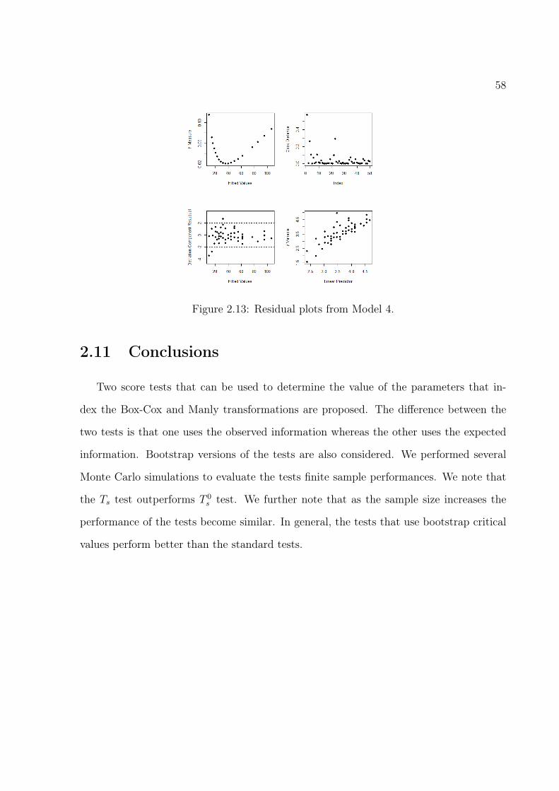
Figures 2.10 to 2.13 contain residual plots of Models 1 through 4, respectively. The
transformation models reduced homoskedasticy deviations relative to the standard and
gamma models, specially when the Manly transformation was used. We observe that the
outlier described above is an influent observation and not a leverage point. The model
that uses the Manly transformation was the model with the best residual plots.
Page 57
56
Figure 2.9: QQ-plots with envelopes.
Figure 2.10: Residual plots from Model 1.
Page 58
57
Figure 2.11: Residual plots from Model 2.
Figure 2.12: Residual plots from Model 3.
Page 59
58
Figure 2.13: Residual plots from Model 4.
2.11 Conclusions
Two score tests that can be used to determine the value of the parameters that in-
dex the Box-Cox and Manly transformations are proposed. The difference between the
two tests is that one uses the observed information whereas the other uses the expected
information. Bootstrap versions of the tests are also considered. We performed several
Monte Carlo simulations to evaluate the tests finite sample performances. We note that
the Ts test outperforms T 0s test. We further note that as the sample size increases the
performance of the tests become similar. In general, the tests that use bootstrap critical
values perform better than the standard tests.
Page 60
CHAPTER 3
Fast double bootstrap
3.1 Resumo
Os recentes avanços na computação possiblilitam o uso de métodos computacionais
intensivos. Boostrap é comumente usado para testes de hipóteses e vêm se mostrando
muito útil. Melhoras na precisão dos testes podem ser obtidas utilizando o fast double
bootstrap. Neste capítulo, utilizamos este método nos testes escore para a estimação do
parâmetro que indexa a transformação da resposta no modelo de regressão linear. Consi-
deramos a transformação de Box-Cox e a transformação de Manly. Evidências numéricas
mostraram que o fast double bootstrap é, em geral, superior ao teste padrão bootstrap.
Palavras-chave: Bootstrap; Fast Double Bootstrap; Transformação de Box-Cox; Trans-
formação de Manly; Teste escore.
59
Page 61
603.2 Abstract
The recent increasing advances in computing power makes it possible to use computer
intensive methods. Bootstrap is commonly used for hypothesis testing and has proven
to be very useful. Improvements in accuracy can be achieved by using is the fast dou-
ble bootstrap. We used this approach for the score test on the parameter that indexes
the response transformation in the linear regression model. We consider the Box-Cox
transformation and also the Manly transformation. Our numerical evidence show that,
in general, the fast double bootstrap test is superior to the standard bootstrap test.
keywords: Bootstrap; Box-Cox transformation; Fast double bootstrap; Manly transfor-
mation; Score test.
3.3 Introduction
Regression analysis is of extreme importance in many areas, such as engineering,
physics, economics, chemistry, medicine, among others. Although the classic linear regres-
sion model is commonly used in empirical analysis, its assumptions are not always valid.
For instance, the normality and homoskedasticy assumptions are oftentimes violated. An
alternative is to use transformation of the response variable.
Hypothesis tests are used to determine whether a parameter equals a given value.
They often make use of large sample approximations. Such approximations can be quite
inaccurate in small samples. An alternative lies in the use of bootstrap resampling, as
introduced by Efron (1979). Data resampling is used to estimate the test statistical null
distribution, from which a more accurate critical value can be obtain. In this chapter
we shall consider the fast double bootstrap in order to improve the accuracy of testing
inferences based on the score tests developed in Chapter 2.
Page 62
613.4 Score test for λ
Regression analysis is used to model the relationship between variables in nearly all
areas of knowledge. In regression analysis we study the dependence of a variable of inte-
rest (response) on a set of independent variables (regressors, covariates). In what follows,
we shall consider the linear regression model.
Let y1, . . . , yT be independent random variables. The model is given by
yt = β1 + β2xt2 + β3xt3 + · · ·+ βpxtp + εt, t = 1, . . . , T, (3.1)
where yt is the tth response, xt2, . . . , xtp are the tth observations on the p − 1 (p < T )
regressors, β1, . . . , βp are the unknown parameters and εt is the tth error.
Oftentimes the response is transformed. The most commonly used transformations
are indexed by a scalar parameter. It is important to perform statistical inference on such
a parameter. Consider the model described in Equation (3.1). In Chapter 2 we proposed
score tests to the parameters that index the Box-Cox and Manly transformations. For
the Box-Cox transformation, the transformation of the response variable is given by
yt(λ) =
yλt −1λ
, if λ 6= 0
log(yt) , if λ = 0.
Suppose we wish to test H0 : λ = λ0 versus H1 : λ 6= λ0. The first score test statistic
is
Ts(λ0) =Sp(λ0)
$[β(λ0), σ2(λ0), λ0],
where Sp(λ0) is the fuction score function evaluated at λ0 and $[β(λ0), σ2(λ0), λ0] is the
asymptotic variance of S(λ) based on the expected information.
We can alternatively use the observed information matrix, i.e., we replace the elements
Page 63
62of the information matrix by the elements of observation matrix. In this case the variance
of Sp(λ) cannot be guaranteed to be positive. The second score test statistic that is
proposed is given by
T 0s (λ0) =
Sp(λ0)
κ[β(λ0), σ2(λ0), λ0],
where Sp(λ0) is the score function evaluated at λ0 and κ[β(λ0), σ2(λ0), λ0] is the estimated
asymptotic variance of S(λ) based on the observed information.
We shall now present two score tests for the parameter that indexes the Manly trans-
formation. The advantage of this transformation is that it can be applied to responses
that assume negative values. Consider the model given in Equation (3.1). By applying
the Manly transformation to the response variable we get
yt(λ) =
eytλ−1λ
, if λ 6= 0
yt , if λ = 0.
The test statistics are given by
Ts(λ0) =Sp(λ0)
$[β(λ0), σ2(λ0), λ0]
and
T 0s (λ0) =
Sp(λ0)
κ[β(λ0), σ2(λ0), λ0].
3.5 Double bootstrap and fast double bootstrap tests
Our interest lies in testing H0 : λ = λ0 versus H1 : λ 6= λ0. The standard score tests
use asymptotic (approximate) critical values. An alternative approach is to use bootstrap
Page 64
63resampling to obtain an estimated critical value. The idea behind the bootstrap method
is to take the initial sample as if it are the population and then generate B artificial
samples from the initial sample (Efron, 1979). Bootstrap resampling can be performed
parametrically or non-parametrically. The parametric bootstrap is used when we are
willing to assume a distribution for y. The non-parametric bootstrap is used when no
distributional assumption is to be made. We shall consider the parametric bootstrap.
When performing bootstrap resamping we impose the null hypothesis. The bootstrap
test is performed as follows (we use the Ts statistic as an example):
• Consider a set of observations, on the response y and on the covariates x2, . . . , xp;
• Compute y(λ0);
• Regress y(λ0) on X, obtain the model residuals, β(λ0) and σ2(λ0) and calculate
Ts(λ0);
• Generate B artificial samples as follows: y∗t (λ0) = xt>β(λ0) + σ(λ0)ε
∗t , where ε∗t
iid∼
N(0, 1);
• For each artificial sample, regress y∗t (λ0) on X, obtain β∗(λ0) and σ2∗(λ0) and com-
pute T ∗s (λ0);
• Obtain the level α bootstrap critical value (BCV1−α) as the (1 − α) quantile of
T ∗s1(λ0), . . . , T∗sB(λ0);
• Reject H0 if Ts(λ0) > BCV(1−α).
It’s plausible to assume that, since bootstrap resampling leads to more precise testing
inferences, bootstrapping a quantity that has already been resampled will lead to a further
improvement in accuracy. This idea was introduced by Beran (1988) for the double
bootstrap (DB). It works as follows (we use the Ts statistic as an example):
• Consider a set of observations, on the response y and on the covariates x2, . . . , xp;
Page 65
64• Compute y(λ0);
• Regress y(λ0) on X, obtain the model residuals, β(λ0) and σ2(λ0) and compute
Ts(λ0);
• Generate B1 first level bootstrap samples as follows: y∗t (λ0) = X>β(λ0) + σ(λ0)ε∗t ,
where ε∗tiid∼ N(0, 1);
• For each artificial sample regress y∗t (λ0) on X, obtain β∗(λ0) and σ2∗(λ0) and com-
pute T ∗s (λ0);
• For each first level pseudo-sample, generate B2 second level bootstrap samples as
follows: y∗∗t (λ0) = x>t β∗(λ0) + σ∗(λ0) + ε∗t ;
• For each second level bootstrap sample, regress y∗∗t (λ0) on X. Obtain β∗∗(λ0) and
σ2∗∗(λ0) and compute T ∗∗s (λ0);
• Compute the first level bootstrap p-value as follows:
p∗(Ts) =1
B1
B1∑i=1
Id(T ∗si > Ts);
• Compute B1 second level p-values as follows:
p∗∗(Ts) =1
B2
B2∑i=1
I(T ∗∗si > T ∗s );
• Compute the double bootstrap p-values as follows:
p∗∗D (Ts) =1
B1
B1∑i=1
Id(p∗j ≤ p∗∗(Ts));
• Reject H0 if p∗∗D (Ts) < α.
Here Id(·) denotes the indicator function. This test is computationally demanding,
since one needs to compute 1+B1×B2 statistics. It would be useful to consider bootstrap
Page 66
65schemes that are less computer intensive.
A way to reduce the computational cost of the double bootstrap was proposed by
Davidson and Mackinnon (2007): the fast double bootstrap (FDB). It is much less
computationally demanding than performing double bootstrap, because we only need to
compute only 1 + 2B1 statistics. The general idea behind the fast double bootstrap is to
only generate one second level bootstrap sample for each first level bootstrap sample. It
works as follows (we use the Ts statistic as an example):
• Consider a set of observations, on the response y and on the covariates x2, . . . , xp;
• Compute y(λ0);
• Regress y(λ0) on X, obtain the model residuals, β(λ0) and σ2(λ0) and compute
Ts(λ0);
• Generate B1 first level bootstrap samples as follows: y∗t (λ0) = X>β(λ0) + σ(λ0)ε∗t ,
where ε∗tiid∼ N(0, 1);
• For each artificial sample regress y∗t (λ0) on X, obtain β∗(λ0) and σ2∗(λ0) and com-
pute T ∗s (λ0);
• Compute the first level bootstrap p-value:
p∗(Ts) =1
B1
B1∑i=1
(T ∗si > Ts);
• For each first level bootstrap generate one second level bootstrap sample as follows:
y∗∗t (λ0) = x>t β∗(λ0) + σ∗(λ0) + ε∗t ;
• For each second level bootstrap sample, regress yt(λ0)∗∗ on X, obtain β∗∗(λ0) and
σ2∗∗(λ0) and compute T ∗∗s (λ0);
• Obtain the 1− p∗ quantile of T ∗∗s1 , . . . , T ∗∗sb1 , Q∗∗B (1− p∗(Ts));
Page 67
66• Compute the fast double bootstrap p-value as follows:
p∗∗FD(Ts) =1
B1
B1∑i=1
(T ∗si > Q∗∗B (1− p∗(Ts)));
• Reject H0 if p∗∗FD(Ts) < α.
3.6 Simulation results
The finite sample performances of the score tests in the linear regression model shall
now be evaluated using Monte Carlo simulations. We consider two transformations: Box-
Cox and Manly. Our goal lies in testing H0 : λ = λ0 versus H1 : λ 6= λ0, where λ is the
parameter that indexes the transformation. The results are based on 10, 000 Monte Carlo
replications with sample sizes T = 20, 40, 60, 80 and 100. We consider a model with two
regressors
yt = β1 + β2xt2 + β3xt3 + εt, t = 1, . . . , T,
where yt is the tth response, xt2 and xt3 are the tth observations on the first and sec-
ond regressors, respectively, β1, β2 and β3 are the unknown parameters and εt is the
tth random error. The covariates values are randomly generated from the U(1, 6) and
N(5, 1) distributions, respectively. For this we used the pseudo-random numbers gen-
erator develop by Marsaglia (1997). The covariate values are kept constant throughout
the simulation. In the Monte Carlo scheme, the errors are generated from the standard
normal distribution. The values of λ0 used are λ0 = 0, 0.5, 1, 1.5 and 2 for the Manly
transformation and λ0 = −1,−0.5, 0, 0.5 and 1 for the Box-Cox transformation. When
λ0 is negative, the true value of β is β = (−8.0,−1.25,−3)>, and when λ0 is not negative
we used β = (8.0, 1.25, 3)>. All the simulations are performed using the on Ox matrix
programming language (Doornik and Ooms (2006)).
Page 68
67
3.6.1 Tests sizes
The tests null rejection rates are computed for each sample size, at the 1%, 5% and 10%
nominal levels, using approximate critical values obtained from the χ21 distribution. The
values of the response variable are generate using λ = λ0, i.e., the tests sizes are estimated
by simulation. For each Monte Carlo replication we performed 500 bootstrap replications.
Tables 3.1 through 3.5 contain the null rejection rates of the score tests on the Box-
Cox transformation parameter with λ = −1,−0.5, 0, 0.5 and 1, respectively. Tables 3.6
through 3.10 contain the null rejection rates of the score tests for the Manly transforma-
tion with λ = 0, 0.5, 1, 1.5 and 2, respectively. Overall, the results show that the bootstrap
tests outperforms the corresponding asymptotic tests. For example, in Table 3.2 the rejec-
tion rates of the Ts test, for T = 20 and at the 5% nominal level are, 0.0584 (asymptotic),
0.0543 (standard bootstrap) and 0.0517 (fast double bootstrap). For the T 0s and Ts tests
in small samples the fast double bootstrap outperforms the standard bootstrap. For the
Ts test with Box-Cox transformation, in large samples, the standard bootstrap outper-
forms fast double bootstrap. For example, in Table 3.2, the rejection rates of the Ts test,
for n = 100 at the 10% nominal level, were 0.9999 and 0.0968, for the standard bootstrap
and fast double bootstrap, respectively.
For both transformations, we can compare Ts asymptotic test to Ts standard boot-
strap test. The asymptotic performs better than the standard bootstrap test. But, in
general, the fast double bootstrap outperforms the others versions. For example, in Table
3.3, for T = 100 at 1% nominal level, the statistic Ts values were, respectivery, 0.0108
(asymptotic), 0.0127 (standard bootstrap) and 0.0105 (fast double bootstrap).
When we compare the standard bootstrap test to the fast double bootstrap test, in
Page 69
68general, the latter typically outperforms the former. For example, in Table 3.6 the rejec-
tion rates of the T 0s test for T = 60 and at the 10% nominal level are 0.1040 (bootstrap)
and 0.1004 (fast double bootstrap). As the sample size increases the null rejection rates
of both of bootstrap tests approach the corresponding nominal levels. The computational
cost of using the fast double bootstrap is approximately 30% higher than that of the usual
bootstrap.
Table 3.1: Null rejetion rates, Box-Cox transformation, λ = −1.Asymptotic Test Boot Test FDBoot Test
Sample size α Ts T 0s Ts T 0
s Ts T 0s
0.01 0.0148 0.0521 0.0140 0.0122 0.0112 0.011220 0.05 0.0582 0.1135 0.0543 0.0533 0.0528 0.0524
0.10 0.1116 0.1748 0.1040 0.1031 0.1050 0.10310.01 0.0115 0.0258 0.0133 0.0137 0.0119 0.0111
40 0.05 0.0505 0.0776 0.0529 0.0526 0.0521 0.05190.10 0.1001 0.1307 0.1037 0.1021 0.1042 0.09980.01 0.0116 0.0201 0.0114 0.0124 0.0105 0.0120
60 0.05 0.0513 0.0667 0.0511 0.0505 0.0517 0.05210.10 0.1022 0.1200 0.0997 0.1033 0.0981 0.10110.01 0.0113 0.0147 0.0128 0.0116 0.0115 0.0102
80 0.05 0.0500 0.0607 0.0510 0.0514 0.0517 0.05060.10 0.0983 0.1113 0.0994 0.1004 0.0982 0.09830.01 0.0104 0.0132 0.0119 0.0114 0.0098 0.0107
100 0.05 0.0488 0.0550 0.0502 0.0505 0.0480 0.04900.10 0.0992 0.1061 0.1001 0.0982 0.0967 0.0964
3.6.2 Tests powers
We shall now evaluate the tests non-null behaviors. The power of a test is the pro-
bability that it rejects the null hypothesis when such a hypothesis is false. We tested
H0 : λ = 1 versus H1 : λ 6= 1. For test this hypothesis, the data were generated using
λ = 1.05, 1.10, 1.15, 1.2, 1.25, 1.30, 1.35, 1.40, 1.45, 1.50. The sample size used was T = 40
and the nominal level is 5%.
Page 70
69
Table 3.2: Null rejetion rates, Box-Cox transformation, λ = −0.5.Asymptotic Test Boot Test FDBoot Test
Sample size α Ts T 0s Ts T 0
s Ts T 0s
0.01 0.0150 0.0520 0.0143 0.0124 0.0125 0.011120 0.05 0.0584 0.1131 0.0541 0.0536 0.0529 0.0524
0.10 0.1120 0.1748 0.1040 0.1033 0.1055 0.10350.01 0.0115 0.0257 0.0134 0.0139 0.0106 0.0111
40 0.05 0.0508 0.0777 0.0528 0.0527 0.0520 0.05200.10 0.1002 0.1305 0.1039 0.1017 0.1045 0.10010.01 0.0116 0.0200 0.0113 0.0124 0.0104 0.0120
60 0.05 0.0513 0.0667 0.0510 0.0504 0.0522 0.05200.10 0.1021 0.1200 0.1000 0.1028 0.0983 0.10100.01 0.0113 0.0147 0.0128 0.0116 0.0116 0.0102
80 0.05 0.0499 0.0607 0.0508 0.0513 0.0517 0.05030.10 0.0986 0.1111 0.0993 0.1002 0.0976 0.09870.01 0.0104 0.0132 0.0119 0.0115 0.0101 0.0107
100 0.05 0.0488 0.0551 0.0500 0.0506 0.0480 0.04910.10 0.0991 0.1061 0.0999 0.0979 0.0968 0.0959
Table 3.3: Null rejetion rates, Box-Cox transformation, λ = 0.Asymptotic Test Boot Test FDBoot Test
Sample size α Ts T 0s Ts T 0
s Ts T 0s
0.01 0.0075 0.0216 0.0102 0.0121 0.0106 0.010520 0.05 0.0415 0.0692 0.0492 0.0469 0.0483 0.0463
0.10 0.0859 0.1236 0.0988 0.0976 0.0986 0.09580.01 0.0105 0.0144 0.0121 0.0124 0.0109 0.0097
40 0.05 0.0533 0.0602 0.0559 0.0517 0.0538 0.05070.10 0.0966 0.1139 0.1036 0.1035 0.1002 0.10210.01 0.0090 0.0124 0.0106 0.0109 0.0084 0.0096
60 0.05 0.0483 0.0548 0.0508 0.0508 0.0504 0.04940.10 0.0981 0.1066 0.1056 0.1044 0.1038 0.10090.01 0.0097 0.0119 0.0109 0.0110 0.0097 0.0098
80 0.05 0.0489 0.0534 0.0502 0.0501 0.0475 0.04830.10 0.0934 0.1030 0.0966 0.0972 0.0951 0.09510.01 0.0108 0.0122 0.0127 0.0126 0.0105 0.0108
100 0.05 0.0478 0.0506 0.0494 0.0494 0.0484 0.04830.10 0.0950 0.1005 0.0987 0.0984 0.0978 0.0978
Page 71
70
Table 3.4: Null rejetion rates, Box-Cox transformation, λ = 0.5.Asymptotic Test Boot Test FDBoot Test
Sample size α Ts T 0s Ts T 0
s Ts T 0s
0.01 0.0139 0.0545 0.0126 0.0129 0.0120 0.012420 0.05 0.0535 0.1146 0.0484 0.0535 0.0519 0.0528
0.10 0.1087 0.1715 0.1002 0.1042 0.1017 0.10390.01 0.0114 0.0251 0.0135 0.0123 0.0120 0.0108
40 0.05 0.0501 0.0764 0.0528 0.0522 0.0520 0.05130.10 0.1011 0.1339 0.1036 0.1033 0.1018 0.10110.01 0.0125 0.0191 0.0138 0.0124 0.0119 0.0105
60 0.05 0.0544 0.0667 0.0520 0.0525 0.0517 0.05230.10 0.1075 0.1204 0.1037 0.1037 0.1015 0.10160.01 0.0106 0.0166 0.0123 0.0133 0.0118 0.0128
80 0.05 0.0554 0.0630 0.0560 0.0539 0.0516 0.05090.10 0.1077 0.1205 0.1072 0.1071 0.1013 0.10140.01 0.0112 0.0130 0.0121 0.0113 0.0119 0.0111
100 0.05 0.0516 0.0599 0.0534 0.0536 0.0518 0.05230.10 0.0994 0.1081 0.1014 0.1000 0.0916 0.1002
Table 3.5: Null rejetion rates, Box-Cox transformation, λ = 1.Asymptotic Test Boot Test FDBoot Test
Sample size α Ts T 0s Ts T 0
s Ts T 0s
0.01 0.0137 0.0547 0.0125 0.0128 0.0120 0.012420 0.05 0.0537 0.1152 0.0484 0.0534 0.0519 0.0536
0.10 0.1084 0.1716 0.1004 0.1039 0.1017 0.10400.01 0.0114 0.0252 0.0136 0.0108 0.0120 0.0103
40 0.05 0.0502 0.1337 0.0527 0.0536 0.0520 0.05290.10 0.1014 0.1032 0.1032 0.1040 0.1018 0.10220.01 0.0126 0.0190 0.0137 0.0124 0.0119 0.0110
60 0.05 0.0543 0.0667 0.0517 0.0525 0.0517 0.05230.10 0.1075 0.1207 0.1036 0.1038 0.1015 0.10080.01 0.0106 0.0166 0.0124 0.0133 0.0118 0.0127
80 0.05 0.0554 0.0630 0.0563 0.0539 0.0519 0.05060.10 0.1074 0.1205 0.1072 0.1073 0.1013 0.10150.01 0.0112 0.0130 0.0120 0.0112 0.0119 0.0116
100 0.05 0.0516 0.0598 0.0532 0.0538 0.0518 0.05210.10 0.0992 0.1082 0.1018 0.0998 0.0986 0.1002
Page 72
71
Table 3.6: Null rejetion rates, Manly transformation, λ = 0.Asymptotic Test Boot Test FDBoot Test
Sample size α Ts T 0s Ts T 0
s Ts T 0s
0.01 0.0142 0.0510 0.0119 0.0133 0.0111 0.011620 0.05 0.0563 0.1105 0.0487 0.0536 0.0468 0.0502
0.10 0.1121 0.1699 0.1000 0.1013 0.0997 0.10130.01 0.0119 0.0238 0.0138 0.0109 0.0109 0.0103
40 0.05 0.0520 0.0743 0.0530 0.0529 0.0517 0.05330.10 0.1038 0.1321 0.1040 0.1035 0.1005 0.10160.01 0.0124 0.0195 0.0128 0.0120 0.0117 0.0114
60 0.05 0.0547 0.0667 0.0542 0.0528 0.0517 0.05090.10 0.1068 0.1200 0.1040 0.1040 0.1004 0.10070.01 0.0116 0.0165 0.0120 0.0130 0.0117 0.0114
80 0.05 0.0542 0.0644 0.0544 0.0550 0.0553 0.05420.10 0.1079 0.1187 0.1090 0.1076 0.1056 0.10850.01 0.0114 0.0134 0.0126 0.0113 0.0099 0.0102
100 0.05 0.0527 0.0588 0.0513 0.0526 0.0490 0.05060.10 0.0989 0.1074 0.1006 0.1002 0.1004 0.0992
Table 3.7: Null rejetion rates, Manly transformation, λ = 0.5.Asymptotic Test Boot Test FDBoot Test
Sample size α Ts T 0s Ts T 0
s Ts T 0s
0.01 0.0139 0.0545 0.0126 0.0129 0.0111 0.011220 0.05 0.0535 0.1146 0.0484 0.0535 0.0460 0.0511
0.10 0.1087 0.1715 0.1002 0.1042 0.1006 0.10220.01 0.0110 0.0234 0.0124 0.0114 0.0114 0.0095
40 0.05 0.0497 0.0741 0.0508 0.0525 0.0491 0.04990.10 0.1288 0.1288 0.1002 0.1015 0.0991 0.09940.01 0.0112 0.0186 0.0128 0.0127 0.0117 0.0108
60 0.05 0.0536 0.0663 0.0529 0.0532 0.0500 0.05140.10 0.1034 0.1198 0.1023 0.1031 0.1002 0.10060.01 0.0133 0.0158 0.0123 0.0119 0.0112 0.0108
80 0.05 0.0526 0.0577 0.0538 0.0538 0.0522 0.05100.10 0.0990 0.1101 0.1003 0.1003 0.1001 0.09870.01 0.0103 0.0144 0.0117 0.0114 0.0110 0.0095
100 0.05 0.0475 0.0539 0.0493 0.0480 0.0481 0.04850.10 0.0982 0.1054 0.0992 0.0979 0.0977 0.0974
Page 73
72
Table 3.8: Null rejetion rates, Manly transformation, λ = 1.Asymptotic Test Boot Test FDBoot Test
Sample size α Ts T 0s Ts T 0
s Ts T 0s
0.01 0.0137 0.0547 0.0125 0.0128 0.0112 0.011620 0.05 0.0537 0.1152 0.0484 0.0534 0.0460 0.0517
0.10 0.1084 0.1716 0.1004 0.1039 0.1005 0.10180.01 0.0114 0.0252 0.0136 0.0123 0.0114 0.0104
40 0.05 0.0502 0.0766 0.0527 0.0523 0.0523 0.05130.10 0.1014 0.1037 0.1032 0.1035 0.1022 0.10170.01 0.0126 0.0190 0.0137 0.0124 0.0114 0.0109
60 0.05 0.0543 0.0667 0.0517 0.0525 0.0514 0.04940.10 0.1075 0.1207 0.1036 0.1038 0.1019 0.10220.01 0.0106 0.0166 0.0124 0.0133 0.0116 0.0122
80 0.05 0.0554 0.0630 0.0563 0.0539 0.0568 0.05330.10 0.1074 0.1205 0.1072 0.1073 0.1048 0.10760.01 0.0112 0.0130 0.0120 0.0112 0.0100 0.0104
100 0.05 0.0516 0.0598 0.0532 0.0538 0.0490 0.05330.10 0.0992 0.1082 0.1018 0.0998 0.1000 0.1001
Table 3.9: Null rejetion rates, Manly transformation, λ = 1.5.Asymptotic Test Boot Test FDBoot Test
Sample size α Ts T 0s Ts T 0
s Ts T 0s
0.01 0.0137 0.0546 0.0126 0.0127 0.0111 0.011520 0.05 0.0537 0.1151 0.0483 0.0534 0.0461 0.0515
0.10 0.1083 0.1716 0.1007 0.1039 0.1007 0.10160.01 0.0114 0.0252 0.0136 0.0123 0.0114 0.0102
40 0.05 0.0502 0.0766 0.0529 0.0526 0.0521 0.05110.10 0.1015 0.1338 0.1033 0.1035 0.1022 0.10170.01 0.0126 0.0190 0.0136 0.0124 0.0114 0.0109
60 0.05 0.0544 0.0670 0.0517 0.0525 0.0514 0.04940.10 0.1074 0.1206 0.1036 0.1038 0.1016 0.10220.01 0.0106 0.0167 0.0124 0.0132 0.0117 0.0121
80 0.05 0.0554 0.0630 0.0565 0.0539 0.0566 0.05300.10 0.1074 0.1203 0.1073 0.1072 0.1049 0.10750.01 0.0112 0.0130 0.0120 0.0112 0.0099 0.0104
100 0.05 0.0517 0.0598 0.0531 0.0539 0.0491 0.05330.10 0.0992 0.1083 0.1018 0.0998 0.0998 0.1002
Page 74
73
Table 3.10: Null rejetion rates, Manly transformation, λ = 2.Asymptotic Test Boot Test FDBoot Test
Sample size α Ts T 0s Ts T 0
s Ts T 0s
0.01 0.0137 0.0546 0.0126 0.0127 0.0111 0.011520 0.05 0.0537 0.1150 0.0484 0.0534 0.0461 0.0514
0.10 0.1082 0.1718 0.1007 0.1039 0.1004 0.10140.01 0.0114 0.0252 0.0136 0.0123 0.0113 0.0101
40 0.05 0.0502 0.0766 0.0529 0.0527 0.0520 0.05110.10 0.1015 0.1338 0.1033 0.1034 0.1023 0.10160.01 0.0126 0.0190 0.0137 0.0126 0.0114 0.0109
60 0.05 0.0545 0.0670 0.0517 0.0525 0.0515 0.04960.10 0.1073 0.1206 0.1036 0.1038 0.1016 0.10260.01 0.0106 0.0167 0.0124 0.0132 0.0117 0.0121
80 0.05 0.0555 0.0630 0.0565 0.0540 0.0566 0.05300.10 0.1074 0.1204 0.1074 0.1073 0.1049 0.10730.01 0.0112 0.0131 0.0120 0.0112 0.0099 0.0104
100 0.05 0.0517 0.0598 0.0530 0.0539 0.0491 0.05320.10 0.0992 0.1082 0.1017 0.0997 0.0997 0.1002
Tables 3.11 and 3.12 contain the powers of the tests on the Box-Cox and Manly trans-
formations, respectively. Comparing the powers of the Ts test with the powers of T 0s test,
we can see that Ts test is more sensitive to small differences between the true λ value and
the λ under H0 than the T 0s test. For example, in Table 3.11, for λ = 1.35 the powers
of the Ts and T 0s tests are 0.9937 and 0.6521, respectively. That also occurs with the
bootstrap versions at the two tests. In general, the use of bootstrap quantile does not
increases the power of the tests.
Page 75
74
Table 3.11: Power of tests, Box-Cox transformation, T = 40 and λ0 = 1.Asymptotic Test Boot Test FDBoot Test
λ Ts T 0s Ts T 0
s Ts T 0s
1.05 0.1158 0.0296 0.1213 0.0246 0.1150 0.02441.01 0.1526 0.0633 0.1531 0.0518 0.1488 0.04951.15 0.7399 0.0964 0.7436 0.0773 0.7231 0.08181.20 0.9016 0.2040 0.9050 0.1700 0.8940 0.17111.25 0.9381 0.3477 0.9390 0.3161 0.9314 0.31391.30 0.9870 0.5097 0.9870 0.4598 0.9847 0.43061.35 0.9937 0.6521 0.9938 0.5746 0.9920 0.53311.40 1.0000 0.8555 1.0000 0.7896 1.0000 0.71871.45 1.0000 0.9743 1.0000 0.9374 1.0000 0.86351.50 0.9999 0.9633 0.9999 0.9358 0.9999 0.8863
Table 3.12: Power of tests, Manly transformation, T = 40 and λ0 = 1.Asymptotic Test Boot Test FDBoot Test
Sample size Ts T 0s Ts T 0
s Ts T 0s
1.05 0.1484 0.0103 0.1568 0.0118 0.1554 0.01261.01 0.2189 0.0322 0.2213 0.0379 0.2160 0.03691.15 0.9149 0.0373 0.9149 0.0397 0.9066 0.03811.20 0.9875 0.0488 0.9886 0.0721 0.9874 0.07471.25 0.9918 0.1239 0.9922 0.1788 0.9905 0.17451.30 0.9999 0.2187 0.9999 0.3161 0.9999 0.29751.35 1.0000 0.3876 1.0000 0.4662 0.9999 0.43061.40 1.0000 0.6363 1.0000 0.7118 1.0000 0.63671.45 1.0000 0.8786 1.0000 0.8964 1.0000 0.79231.50 1.0000 0.9247 1.0000 0.9413 1.0000 0.8666
3.7 Conclusions
In this chapter we presented the fast double bootstrap scheme for the score tests deve-
loped in Chapter 2. We performed Monte Carlo simulations using 500 first level bootstrap
replications and one second order level bootstrap replication.
Comparing the standard bootstrap test to the fast double bootstrap test we note that,
in general, FDB outperforms standard bootstrap. The difference is subtle and the com-
putational cost of using the fast double bootstrap is, on average, 30% higher. The use of
bootstrap quantile does not increases the power of the tests.
Page 77
CHAPTER 4
Estimators of the transformation parameter via normality tests
4.1 Resumo
O modelo de regressão linear é frequentemente usado em diferentes áreas do conheci-
mento. Muitas vezes, no entanto, alguns pressupostos são violados. Uma possível solução
é transformar a variável resposta. Para estimar os parâmetros que indexam as transfor-
mações de Box-Cox e Manly, propusemos sete estimadores não-paramétricos baseados em
testes de normalidade. Realizamos simulações de Monte Carlo em três casos. Caso 1, para
transformar uma variável não normal, caso 2, para transformar a resposta do modelo de
regressão linear quando a suposição de normalidade não é violada e caso 3, para transfor-
mar a variável resposta do modelo de regressão linear quando a suposição de normalidade
é violada. Comparamos os resultados com o estimador de máxima verosimilhança (EMV)
e, no caso 3, há pelo menos um estimador não-paramétrico com melhor desempenho do
que o EMV. Uma aplicação empírica é apresentada e discutida.
keywords: Monte Carlo; Transformação de Box-Cox; Transformação de Manly; Testes
76
Page 78
77de Normalidade.
4.2 Abstract
The linear regression model is frequently used in empirical applications in many di-
fferent fields. Oftentimes, however, some of the relevant assumptions are violated. A
possible solution is to transform the response variable. To estimate the parameters that
index the Box-Cox and Manly transformations we propose seven nonparametric estima-
tors based on normality tests. We perform Monte Carlo simulations in three cases. First,
to transform a non-normal variable, second to transform the response variable of a linear
regression model when the assumption of normality is not violated and third to transform
the response variable of a linear regression model when the assumption of normality is
violated. We compare the proposed estimators finite sample behavior to that of the maxi-
mum likelihood estimator (MLE) and, in case three, at least one nonparametric estimator
outperform MLE. An empirical application is presented and discussed.
keywords: Box-Cox transformation; Manly transformation; Monte Carlo simulation;
Normality tests.
4.3 Introduction
A great deal of statistical inferences rely on the assumption that the data generating
process is Gaussian. Such an assumption is, however, oftentimes violated in empirical
applications. Data transformations that are able to reduce deviations from normality are
thus quite useful. The most popular transformation is the Box-Cox transformation (Box
and Cox, 1964). It covers both the logarithmic transformation and the no transforma-
tion case. The Box-Cox transformation, however, has a limitation: it requires that the
variable only assumes positive values. There are alternative transformations that can be
Page 79
78used when the variable assumes negative values, such as the Manly (Manly, 1976) and
the Bickel and Doksum transformations (Bickel and Doksum, 1981).
Estimation of the parameter that indexes the transformation is crucial. Box and Cox
(1964) proposed that the Box-Cox transformation parameter be estimated by maximum
likelihood (ML). Rahman (1999) and Rahman and Pearson (2008) proposed estimating
the Box-Cox transformation parameter via the Shapiro-Wilk and Anderson-Darling nor-
mality tests, respectively. They use the Newton-Raphson (N-R) algorithm to obtain the
Box-Cox transformation parameter estimate. A disadvantage of N-R algorithm is that
it requires the specification of a starting value and it might stop at a local (not global)
maximum. Asar et al. (2015) estimated the Box-Cox transformation parameter with an
algorithm which selects a value belonging to a predetermined interval. They considered
estimation based on seven normality tests, maximizing its p-values to this interval.
The chief goal of this chapter is to consider estimation of the Manly transformation
parameter via normality tests. Additionally, we shall use the same approach to estimate
the parameter that indexes the transformation in the linear regression model. For that
case, we shall consider both the Box-Cox and the Manly transformations.
4.4 Transformations
The most well known data transformation is the Box-Cox transformation (Box and
Cox, 1964). Let y1, . . . , yT be independent random variables. The transformation is given
by
yt(λ) =
yλt −1λ
, if λ 6= 0
log (yt) , if λ = 0.
Page 80
79The transformation parameter (λ) usually assumes values between −2 and 2. The
popularity of this transformation is due to the fact that it includes as special cases both
the no transformation case (λ = 1) and the logarithmic transformation (λ = 0). The
main disadvantage of the Box-Cox transformation is that it can only be applied to pos-
itive data. Another disadvantage lies in the fact that the transformed variable becomes
bounded (except for λ = 0 and λ = 1).
A useful alternative to the Box-Cox transformation that can be used with negative
data is the Manly transformation (Manly, 1976). It has been shown to be quite effective
in transforming unimodal distributions into nearly symmetrical ones (Manly, 1976). The
transformed variable is
yt(λ) =
eλyt−1λ
, if λ 6= 0
yt , if λ = 0.
Similar to the Box-cox transformation, the transformed variable is bounded. Another
disadvantage of both transformations is that inferences made after the variable has been
transformed are conditional on the selected value of λ and thus neglect the uncertainty
involved in the estimation of λ.
4.5 Some well-known normality tests
In this section we shall present some normality tests that can be used to test H0: y
follow a normal distribution versus H1: y does not follow a normal distribution.
4.5.1 Shapiro-Wilk test
The Shapiro-Wilk test was proposed by Shapiro and Wilk (1965). The test statistic
W is calculated by dividing the square of a linear combination of the order statistics by
Page 81
80the variance estimator. It is especially sensitive to asymmetry and long tails. The test
statistic is given by
W =(∑T
t=1 aty(t))2∑T
t=1(yt − y)2,
where y(t) is the tth order statistic and y is the sample mean. The constants at are
(a1, . . . , aT )> =m>V −1
(m>V −1V −1m)12
,
where m = (m1, . . . ,mT )> is a vector of the expected values of the order statistic of
independent and identically distributed random variables that follow the standard normal
distribution and V being the covariate matrix of those order statistics. This test has the
disadvantage that its critical values have to be obtained from tables, which are available
in Shapiro and Wilk (1965) for sample sizes smaller than 50. To solve this problem one
can use the algorithm developed by Royston (1982) to calculate the test p-values with
sample sizes that does not exceed 2000.
4.5.2 Shapiro-Francia test
When the sample size is large, a slight modification of the Shapiro-Wilk test can be
used. It is the Shapiro-Francia test (Shapiro and Francia, 1972). The test statistic is
W =
∑Tt=1mty(t)
(T − 1)σ2∑T
t=1m2t
,
where m = (m1, . . . ,mT )> is a vector of the expected values of the order statistic of
independent and identically distributed random variables that follow the standard normal
distribution and σ2 is the sample variance. The relevant quantiles of the null distribution
ofW are available in Shapiro and Francia (1972). Royston (1993) developed an algorithm
that can be used to compute the test p-values with sample sizes smaller than 5000.
Page 82
814.5.3 Kolmogorov-Smirnov test
The distance between the null distribution and the empirical distribution function
(EDF) is a natural quantity to assess the goodness of fit. This idea was explored by
Kolmogorov (1933). Let G be the postulated distribution function and let F be the
distribution function.
Our interest lies in testing the null hypothesis H0 : F = G versus H1 : F 6= G. Smirnov
(1939) developed the test that became known as the Kolmogorov-Smirnov test. The test
statistic is given by DT = max(D+T , D
−T ), where
D+T =√T supt=1,...,T
(Ft(y)−G(y)),
D−T =√T supt=1,...,T
(G(y)− Ft(y)),
where F is the empirical distribution, D+T is the largest positive deviation and D−T is the
large negative deviation. The computation of these quantities requires the evaluation of G
and F at many points (Thas, 2009). Since Ft(y) is a step function and G(y) is a monotone
increasing function, D+T and D−T , simplify to
D+T = max
t=1,...,T
(1
T−G(y(t))
),
D−T = maxt=1,...,T
(G(y(t))−
t− 1
T
),
respectively. DT is distribution free, i.e., for any hypothesized distribution, its null dis-
tribution is the same, even in finite samples (Thas, 2009). The critical values of the test
are available in Massey (1951) for samples sizes up to 35. Based on the asymptotic null
distribution of DT one can compute the test p-values using the algorithm developed by
Dallal and Wilkinson (1986).
Page 83
824.5.4 Lilliefors test
Lilliefors (1967) was the first to tabulate the quantiles from the null distribution of
Kolmogorov-Smirnov test for testing normality. The test is often named after Lilliefors.
The test statistic is given by DT = max{D+T , D
−T }, where
D+T = max
t=1,...,T
(t
T−G(y(t))
),
D−T = maxt=1,...,T
(G(y(t))−
t− 1
T
).
The exact quantiles of the null distribution of DT were tabulated by Massey (1951)
for sample sizes up to 35. For larger samples, Marsaglia et al. (2003) proposed a method
that can be used to approximate the test statistic asymptotic null distribution while can
be used to compute test p-values.
4.5.5 Anderson-Darling test
A class of test statistics based on the distance between the null distribution and the
empirical distribution was proposed by Anderson and Darling (1954).
Qt =
∫ +∞
−∞w(G(y))IB2
tdG(y), (4.1)
where w(·) is some non-negative weight function chosen to accentuate the sensibility of
the test and B is the distance between F and G. When w(u) = 1/u(1− u), we have the
Anderson-Darling statistic. For such a weight function, the test statistic is
A = −T −T∑t=1
2t− 1
T(logG(y(t)) + log(1−G(y(T+1−t)))).
The exact null distribution of A cannot be easily obtained. Asymptotic critical values
were tabulated by Stephens (1986).
Page 84
834.5.6 Cramér-Von Mises test
Using w(u) = 1 (∀ 0 ≤ u ≤ 1) in Equation (4.1), one obtain the statistic test proposed
by Cramér (1928):
W =1
12T+
T∑t=1
(G(y(t))−
2t− 1
2T
)2
.
As with the Anderson-Darling test, the test statistic exact null distribution cannot be
easily obtained and its null quantiles were tabulated only for sample sizes smaller than 7.
Stephens (1986) derived the asymptotic null distribution of W .
4.5.7 Pearson chi-square test
The Pearson chi-square test was developed to test multinomial distributions, but it is
also used to test continuous distributions (Thas, 2009). Suppose we have T observations
which can be classifiend into k classes. Let Oi denotes the count of observations in class i,
(i = 1, . . . , k). Clearly, we have that∑k
i=1Oi = T . Under null hypothesis, the probability
that a given observation belongs to the class i is pi. So, the test statistic is
χ2 =k∑i=1
(Oi − Tpi)2
Tpi.
The test statistic asymptotic null distribution is χ2k−1.
4.5.8 Bera-Jarque test
Most normality tests are based on the comparison between the empirical cumulative
distribution and the theoretical normal cumulative distribution or are based on the com-
parison between the empirical quantiles and the theoretical normal quantiles. In contrast,
Bera and Jarque (1987) proposed a normality test based on the sample skewness and on
the sample kurtosis. The test exploit the fact that the normal distribution is symmetric
Page 85
84and its kurtosis coefficient equals three. We test these two conditions simultaneity. The
test statistic is
BJ = T
(s2
6+
(h− 3)2
24
),
where s =∑Tt=1 (yt−µt)3
T (σ2)32
is the skewness coefficient and k =∑Tt=1 (yt−µt)
4
T (σ2)2. The test statistic
asymptotic null distribution is χ22.
4.6 Simulation setup
Asar et al. (2015) used seven normality tests to select the value of the parameter that
indexes the Box-Cox transformation. Using a similar approach, we developed seven esti-
mators for the parameters that index the Box-Cox and Manly transformations in three
cases: case 1, to transform a continuous variable, case 2, to transform the response of
the linear model when the normality assumption is not violated and case 3, when the
normality assumption is violated.
Let y1, . . . , yT be independent random variables. The linear regression model is given
by
yt = β1 + β2xt2 + β3xt3 + · · ·+ βpxtp + εt, t = 1, . . . , T,
where yt is the tth response, xt2, . . . , xtp are the tth observations on p − 1 (p < T )
regressors which influence the mean of the response, µt = IE(yt), β1, . . . , βp are the un-
known parameters and εt is the tth error. When λ0 is negative, the true value of β is
β = (−8.0,−1.25,−3)>, and when λ0 is not negative we used β = (8.0, 1.25, 3)>. We
consider the following estimators that are obtained from normality tests: Shapiro-Wilk
Estimator (λSW ), Shapiro-Francia Estimator (λSF ), Anderson Darling Estimator (λAD),
Cramér-Von Mises Estimator (λCVM), Pearson Estimator (λP ), Lilliefors Estimator (λL)
Page 86
85and Bera-Jarque Estimator (λBJ).
In what follows we consider the following cases:
Case 1 (continuous variable transformation)
• Generate a (T × 1) vector y from the standard normal distribution;
• Apply the inverse transformation function with λ = λ0 to obtain non-normal data;
• Choose an interval of candidate values for λ;
• Transform y using each λ value in a sequence of values that span the chosen interval;
• Compute the normality test statistic for each value of λ and find the value of λ that
maximizes the test p-value.
Case 2 (response transformation with normality assumption)
• Generate a (T × 1) error vector from the standard normal distribution;
• Obtain yt(λ) = β1 + β2xt2 + · · ·+ βpxtp + εt;
• Apply the inverse transformation using λ = λ0 to obtain yt;
• Choose an interval of candidates values for λ;
• For each value of λ regress yt on xt2, . . . , xtp by ordinary least squares and obtain
β1, . . . , βp and εt, where εt is the tth residual;
• Apply the specified normality test on ε and find the value of λ that yields the largest
p-value.
Case 3 (response transformation without normality assumption)
• Generate a (T × 1) error vector from the central Student’s t with 4 degrees of
freedom;
Page 87
86• Obtain yt(λ) = β1 + β2xt2 + · · ·+ βpxtp + εt;
• Apply the inverse transformation function using λ = λ0 to obtain yt;
• Choose an interval of candidates values of λ;
• For each value of λ regress yt on xt2, . . . , xtp by ordinary least squares and obtain
β1, . . . , βp and εt;
• Apply the specified normality test on ε and find the value of λ that yields the largest
p-value.
4.7 Simulation results
We perform Monte Carlo simulations using 10, 000 replications. For Case 1 we generate
y ∼ N(5, 1) and use the inverse transformation to obtain non-normal data. For Case 2,
we generate x1 ∼ U(1, 6) and ε ∼ N(0, 1) and for Case 3 we generate x1 ∼Normal(0, 1)
and ε ∼ t(4). In the simulations, we consider the model
yt = β1 + β2xt2 + εt, t = 1, . . . , T.
The interval used for the values of λ is [−2, 2]. We coinsider the following sequence
of candidate values for λ : −2.00,−1.95, · · · , 0, · · · , 1.95, 2.00. Our goal lies in testing
H0 : λ = λ0 versus H1 : λ 6= λ0, where λ is the parameter that indexes the transformation.
We consider two transformations: Box-Cox and Manly. The values of λ0 used are λ0 =
0, 0.5, 1, 1.5 and 2 for the Manly transformation and λ0 = −1,−0.5, 0, 0.5 and 1 for the
Box-Cox transformation. The sample sizes are T = 20, 30, 50, 100 and 500. We consider
three cases, which are described in what follows.
Page 88
874.7.1 Case 1: Estimation for a continuous variable
Tables 4.1 through 4.5 contain the biases, variances and mean square errors (MSE) of
the estimators of the Box-Cox transformation parameter with λ = −1,−0.5, 0, 0.5 and 1,
respectively. Tables 4.6 to 4.10 contain the biases, variances and MSEs of the estimators
of the Manly transformation parameter with λ = 0, 0.5, 1, 1.5 and 2, respectively. As
expected, for both transformations, biases, variances and MSEs become smaller as the
sample size increases. For example, in Table 4.1, when T = 20, the bias of λAD equals
1.0077, whereas with T = 500 it equals 0.0006. λMLE is the best performer.
For the Box-Cox transformation, the best performing nonparametric estimator is λSW ,
followed by the λSF and λBJ . For example, in Table 4.2, with T = 30, the MSEs of λSW ,
λSF and λBJ , are, respectively, 0.0825, 0.8500 and 0.8701. λP is the worst performer. In
large samples the nonparametric estimators of λ performed similar to λMLE. For example,
in Table 4.3, for T = 500, the biases of λMLE, λSW , λSF and λBJ are equal to 0.0161,
0.0161, 0.0163 and 0.0264, respectively.
As with Box-Cox transformation, with Manly transformation the best performing es-
timator is λMLE. The best performing nonparametric estimator is λSW , followed by λSF
and λBJ . For example, in Table 4.6 and with T = 50 the MSEs of λMLE, λSW , λSF and
λBJ are 0.0137, 0.0165, 0.0170 and 0.0172, respectively. The worst performing estimators
are λP and λLL. For example, in Table 4.9, the MSEs of λMLE, λSW , λSF and λBJ are,
respectively 0.0900, 0.0854, 0.0858 and 0.0862, whereas, for λP and λLL they are equal
to 0.2169 and 0.1427, respectively. In large samples, the best performed nonparametric
estimators behaved similary to λMLE. For example, in Table 4.7, for T = 500, the MSEs
of λMLE, λSW , λSF and λBJ are 0.0161, 0.0161, 0.0163 and 0.0162, respectively.
Page 89
88
Table 4.1: Biases, variances, MSEs of the estimators of λ (Box-Cox transformation pa-rameter) when λ0 = −1 (Case 1).
T λMLE λSW λSF λAD λCVM λP λL λBJBias 0.1417 0.2232 0.2071 0.2516 0.2279 1.0077 0.3071 0.2490
20 Variance 1.5716 1.2156 1.2404 1.4205 1.3049 1.5646 1.5095 1.2645MSE 1.5917 1.2654 1.2833 1.4838 1.3569 2.5802 1.6039 1.3265
Bias 0.0944 0.1204 0.1047 0.1426 0.1208 0.7094 0.1864 0.138330 Variance 0.9466 0.8222 0.8390 1.0225 0.9122 1.3305 1.1207 0.8510
MSE 0.9555 0.8367 0.8500 1.0428 0.9267 1.8337 1.1554 0.8701
Bias 0.0652 0.0577 0.0405 0.0673 0.0541 0.4080 0.0968 0.073550 Variance 0.5087 0.4971 0.5062 0.6675 0.5832 0.9663 0.7460 0.5130
MSE 0.5130 0.500 0.5079 0.6720 0.5861 1.1328 0.7554 0.5184
Bias 0.0375 0.0214 0.0066 0.0222 0.0167 0.1797 0.0414 0.0335100 Variance 0.2428 0.2500 0.2552 0.3663 0.3150 0.5970 0.4134 0.2538
MSE 0.2443 0.2504 0.2552 0.3668 0.3153 0.6293 0.4151 0.2550
Bias 0.0094 0.0041 −0.0021 0.0006 0.0017 0.0126 0.0035 0.0089500 Variance 0.0444 0.0456 0.0460 0.0750 0.0631 0.1585 0.0872 0.0457
MSE 0.0445 0.0456 0.0460 0.0750 0.0631 0.1587 0.0872 0.0458
Table 4.2: Biases, variances, MSEs of the estimators of λ (Box-Cox transformation pa-rameter) when λ0 = −0.5 (Case 1).
T λMLE λSW λSF λAD λCVM λP λL λBJBias 0.0111 0.1253 0.1122 0.1201 0.1187 0.2728 0.1384 0.1341
20 Variance 0.0367 0.0464 0.0435 0.0716 0.0578 0.2834 0.2034 0.0795MSE 0.0369 0.0621 0.0561 0.0860 0.0719 0.3578 0.2226 0.0974
Bias 0.0257 −0.1452 −0.1743 −0.1428 −0.1451 −0.0258 −0.1250 −0.113530 Variance 0.0525 0.0614 0.0604 0.1172 0.0859 0.3603 0.2361 0.0936
MSE 0.0532 0.0825 0.0908 0.1376 0.1070 0.3609 0.2517 0.1065
Bias 0.0024 0.0574 0.0484 −0.0331 0.0143 0.1001 0.1113 0.012550 Variance 0.0148 0.0179 0.0167 0.0356 0.0258 0.0750 0.1079 0.0609
MSE 0.0148 0.02119 0.0190 0.0367 0.0260 0.0850 0.1203 0.0611
Bias 0.0027 0.1620 0.1510 0.2058 0.1813 0.1075 0.1143 0.2413100 Variance 0.0070 0.0085 0.0082 0.0151 0.0116 0.0344 0.0699 0.0180
MSE 0.0070 0.0347 0.0309 0.0574 0.0445 0.0459 0.0829 0.0762
Bias 0.0008 −0.0074 −0.0107 −0.0041 −0.0118 −0.0072 −0.1498 0.0476500 Variance 0.0016 0.0020 0.0019 0.0042 0.0029 0.0139 0.0119 0.0067
MSE 0.0016 0.0020 0.0020 0.0042 0.0030 0.0140 0.0336 0.0090
Page 90
89
Table 4.3: Biases, variances, MSEs of the estimators of λ (Box-Cox transformation pa-rameter) when λ0 = 0 (Case 1).
T λMLE λSW λSF λAD λCVM λP λL λBJBias −0.0032 −0.0034 −0.0035 −0.0032 −0.0034 0.0860 −0.0027 −0.0043
20 Variance 0.0466 0.0628 0.0648 0.0874 0.0738 0.1768 0.1066 0.0743MSE 0.0466 0.0628 0.0648 0.0874 0.0738 0.1842 0.1066 0.0744
Bias −0.0028 −0.0031 −0.0030 −0.0033 −0.0036 0.0443 −0.0035 −0.003230 Variance 0.0268 0.0327 0.0339 0.0467 0.0390 0.0962 0.0565 0.0356
MSE 0.0268 0.0327 0.0339 0.0468 0.0390 0.0982 0.0565 0.0356
Bias 0.0005 0.0003 0.0006 −0.0004 −0.0003 0.0190 0.0000 0.000050 Variance 0.0149 0.0173 0.0179 0.0256 0.0213 0.0492 0.0296 0.0181
MSE 0.0149 0.0173 0.0179 0.0256 0.0213 0.0496 0.0296 0.0180
Bias −0.0005 −0.0007 −0.0006 −0.0003 −0.0003 0.0066 −0.0000 −0.0007100 Variance 0.0066 0.0075 0.0077 0.0116 0.0096 0.0240 0.0137 0.0077
MSE 0.0067 0.0075 0.0077 0.0116 0.0097 0.0240 0.0137 0.0077
Bias −0.0008 −0.0011 −0.0011 −0.0007 −0.0007 0.0001 −0.0003 −0.0010500 Variance 0.0012 0.0016 0.0016 0.0024 0.0020 0.0048 0.0026 0.0016
MSE 0.0013 0.0016 0.0016 0.0024 0.0020 0.0048 0.0026 0.0016
Table 4.4: Biases, variances, MSEs of the estimators of λ (Box-Cox transformation pa-rameter) when λ0 = 0.5 (Case 1).
T λMLE λSW λSF λAD λCVM λP λL λBJBias −0.0176 −0.0317 −0.0189 −0.0226 −0.0220 0.184040 −0.0497 −0.0439
20 Variance 0.4574 0.6400 0.6613 0.8042 0.7141 1.0423 0.8784 0.6846MSE 0.4577 0.6410 0.6617 0.8047 0.7146 1.0761 0.8809 0.6865
Bias −0.0436 −0.0340 −0.0219 −0.0245 0.0248 0.1107 −0.0349 −0.041830 Variance 0.2893 0.3831 0.3963 0.5282 0.4499 0.8440 0.6106 0.4089
MSE 0.2912 0.3843 0.3968 0.5288 0.4505 0.8562 0.6118 0.4107
Bias −0.0337 −0.0080 0.0020 0.0025 0.0021 0.0765 −0.0030 −0.015450 Variance 0.1709 0.1961 0.2021 0.2962 0.2449 0.5336 0.3455 0.2063
MSE 0.1720 0.1962 0.2021 0.2962 0.2449 0.5395 0.3455 0.2066
Bias −0.0331 −0.0111 −0.0038 −0.0008 −0.0034 0.02112 −0.0026 −0.0166100 Variance 0.0889 0.0878 0.0901 0.1350 0.1120 0.2745 0.1561 0.0894
MSE 0.0900 0.0879 0.0901 0.1350 0.1119 0.2750 0.1561 0.0897
Bias −0.0041 −0.0011 0.0019 0.0004 0.0001 −0.0030 0.0000 −0.0034500 Variance 0.0158 0.0161 0.0164 0.0254 0.0212 0.0543 0.0296 0.0162
MSE 0.0158 0.0161 0.0164 0.0254 0.0212 0.0543 0.0296 0.0162
Page 91
90
Table 4.5: Biases, variances, MSEs of the estimators of λ (Box-Cox transformation pa-rameter) when λ0 = 1 (Case 1).
T λMLE λSW λSF λAD λCVM λP λL λBJBias 0.0386 −0.2201 −0.2054 −0.2538 −0.2272 −0.1446 −0.3029 −0.2462
20 Variance 0.9707 1.2252 1.2475 1.4229 1.3123 1.3461 1.4897 1.2734MSE 0.9721 1.2736 1.2896 1.4873 1.3640 1.3671 1.5814 1.3340
Bias −0.0138 −0.1379 −0.1219 −0.1620 −0.1411 −0.1864 −0.2095 −0.155530 Variance 0.6454 0.8521 0.8695 1.0459 0.9416 1.2107 1.1473 0.8743
MSE 0.6456 0.8711 0.8844 1.0722 0.9615 1.2454 1.1912 0.8985
Bias −0.0338 −0.0651 −0.0482 −0.0754 −0.0618 −0.1615 −0.1026 −0.081650 Variance 0.4262 0.5044 0.5151 0.6618 0.5813 0.9276 0.7369 0.5175
MSE 0.4273 0.5086 0.5175 0.6675 0.5851 0.9537 0.7474 0.5242
Bias −0.0299 −0.0194 −0.0048 −0.0168 −0.0132 −0.0815 −0.0319 0.0324100 Variance 0.2218 0.2413 0.2465 0.3579 0.3056 0.5711 0.4056 0.2443
MSE 0.2227 0.2417 0.2465 0.3582 0.3057 0.5777 0.4066 0.2453
Bias −0.0071 −0.0018 0.0049 0.0011 0.0007 0.0024 −0.0022 −0.0062500 Variance 0.0447 0.0458 0.0465 0.0758 0.0633 0.1553 0.0894 0.0464
MSE 0.0448 0.0458 0.0465 0.0758 0.0633 0.1553 0.0894 0.0464
Table 4.6: Biases, variances, MSEs of the estimators of λ (Manly transformation param-eter) when λ0 = 0 (Case 1).
T λMLE λSW λSF λAD λCVM λP λL λBJBias 0.0000 −0.0025 −0.0026 −0.0029 −0.0030 0.0882 −0.0033 −0.0028
20 Variance 0.0444 0.0604 0.0626 0.0829 0.0703 0.1686 0.0992 0.0700MSE 0.0444 0.0604 0.0626 0.0829 0.0703 0.1764 0.0992 0.0701
Bias 0.0034 0.0021 0.0025 0.0008 0.0015 0.0449 0.0011 0.002730 Variance 0.0444 0.0604 0.0626 0.0829 0.0703 0.1686 0.0992 0.0700
MSE 0.0264 0.0336 0.0347 0.0480 0.0402 0.1010 0.0580 0.0376
Bias 0.0004 0.0006 0.0006 0.0001 0.0004 0.0226 −0.0002 0.000850 Variance 0.0137 0.0164 0.0170 0.0245 0.0203 0.0496 0.0296 0.0172
MSE 0.0137 0.0165 0.0170 0.0245 0.0203 0.0501 0.0296 0.0172
Bias −0.0007 −0.0008 −0.0009 −0.0011 −0.0010 0.0047 −0.0006 −0.0008100 Variance 0.0137 0.0165 0.0170 0.0245 0.0203 0.0496 0.0296 0.0172
MSE 0.0064 0.0075 0.0077 0.0114 0.0096 0.0231 0.0133 0.0076
Bias −0.0004 −0.0005 −0.0006 −0.0002 −0.0004 0.0009 −0.0002 −0.0006500 Variance 0.0012 0.0016 0.0016 0.0024 0.0020 0.0046 0.0026 0.0016
MSE 0.0012 0.0016 0.0016 0.0024 0.0020 0.0046 0.0026 0.0016
Page 92
91
Table 4.7: Biases, variances, MSEs of the estimators of λ (Manly transformation param-eter) when λ0 = 0.5 (Case 1).
T λMLE λSW λSF λAD λCVM λP λL λBJBias −0.0192 −0.0363 −0.0231 −0.0325 −0.0289 0.1889 −0.0514 −0.0496
20 Variance 0.4496 0.6312 0.6520 0.8032 0.7098 1.0520 0.8784 0.6750MSE 0.4500 0.6325 0.6525 0.8042 0.7106 1.0877 0.8810 0.6774
Bias −0.0319 −0.0172 0.0060 −0.0053 −0.0061 0.1222 −0.0192 −0.024930 Variance 0.2939 0.3859 0.3988 0.5349 0.4561 0.8385 0.5983 0.4122
MSE 0.2949 0.3862 0.3988 0.5349 0.4561 0.8534 0.5987 0.4128
Bias −0.0346 −0.0109 −0.0002 −0.0058 −0.0043 0.0796 −0.0114 −0.020450 Variance 0.1762 0.2038 0.2101 0.3044 0.2538 0.5423 0.3527 0.2154
MSE 0.1774 0.2039 0.2101 0.3044 0.2538 0.5487 0.3528 0.2158
Bias −0.0358 −0.0127 −0.0054 −0.0035 −0.0051 0.0256 −0.0083 −0.0179100 Variance 0.0907 0.0894 0.0918 0.1366 0.1140 0.2842 0.1610 0.0915
MSE 0.0920 0.0896 0.0918 0.1366 0.1141 0.2848 0.1611 0.0918
Bias −0.0044 −0.0012 0.0020 −0.0004 −0.0004 −0.0020 −0.0011 −0.0035500 Variance 0.0160 0.0161 0.0163 0.0264 0.0220 0.0565 0.0301 0.0162
MSE 0.0161 0.0161 0.0163 0.0264 0.0220 0.0565 0.0301 0.0162
Table 4.8: Biases, variances, MSEs of the estimators of λ (Manly transformation param-eter) when λ0 = 1 (Case 1).
T λMLE λSW λSF λAD λCVM λP λL λBJBias 0.0431 −0.2120 −0.1966 −0.2447 −0.2182 −0.1568 −0.2795 −0.2390
20 Variance 0.9617 1.1969 1.2169 1.4139 1.2953 1.3601 1.4823 1.2557MSE 0.9636 1.2418 1.2555 1.4738 1.3429 1.3847 1.5604 1.3129
Bias −0.0108 −0.1323 −0.1152 −0.1584 −0.1359 −0.1813 −0.1998 −0.154430 Variance 0.6539 0.8262 0.8418 1.0160 0.9144 1.2118 1.1141 0.8515
MSE 0.6540 0.8437 0.8551 0.0411 0.9328 1.2447 1.1540 0.8754
Bias −0.0377 −0.0668 −0.0501 −0.0756 −0.0619 −0.1434 −0.1064 −0.083250 Variance 0.4137 0.4997 0.5108 0.6607 0.5776 0.9191 0.7410 0.5122
MSE 0.4151 0.5041 0.5133 0.6664 0.5815 0.9397 0.7523 0.5191
Bias −0.0382 −0.0291 −0.0149 −0.0269 −0.0228 −0.0892 −0.0412 −0.0424100 Variance 0.2249 0.2480 0.2537 0.3662 0.3119 0.5858 0.4157 0.2514
MSE 0.2263 0.2489 0.2540 0.3669 0.3125 0.5937 0.4174 0.2532
Bias −0.0088 −0.0035 0.0023 0.0010 0.0005 −0.0009 0.0021 −0.0081500 Variance 0.0446 0.0457 0.0464 0.0741 0.0620 0.1551 0.0870 0.0459
MSE 0.0447 0.0457 0.0464 0.0741 0.0620 0.1551 0.0870 0.0459
Page 93
92
Table 4.9: Biases, variances, MSEs of the estimators of λ (Manly transformation param-eter) when λ0 = 1.5 (Case 1).
T λMLE λSW λSF λAD λCVM λP λL λBJBias 0.0013 −0.5581 −0.5453 −0.6164 −0.5755 −0.5977 −0.6730 −0.5894
20 Variance 1.9894 1.5425 1.5563 1.7689 1.6355 1.4822 1.8315 1.6026MSE 1.9894 1.8540 1.8537 2.1489 1.9667 1.8394 2.2844 1.9501
Bias −0.0559 −0.4060 −0.3923 −0.4616 −0.4227 −0.6189 −0.5272 −0.433230 Variance 1.3521 1.0795 1.0891 1.3020 1.1799 1.3504 1.4328 1.1171
MSE 1.3553 1.2444 1.2430 1.5151 1.3586 1.7335 1.7108 1.3048
Bias −0.0696 −0.2586 −0.2433 −0.3227 −0.2844 −0.5953 −0.3847 −0.279850 Variance 0.8669 0.6745 0.6778 0.8719 0.7673 1.1029 0.9927 0.6981
MSE 0.8717 0.7413 0.7370 0.9760 0.8482 1.4573 1.1407 0.7761
Bias −0.0474 −0.1127 0.0987 −0.1598 −0.1324 −0.4224 −0.1821 −0.1292100 Variance 0.4571 0.3420 0.3435 0.4606 0.4011 0.6987 0.5230 0.3491
MSE 0.4593 0.3547 0.3533 0.4861 0.4186 0.8771 0.5562 0.3658
Bias −0.0156 −0.0127 −0.0033 −0.0236 −0.0179 −0.1113 −0.03038 −0.0197500 Variance 0.0898 0.0852 0.0858 0.1278 0.1106 0.2045 0.1418 0.0858
MSE 0.0900 0.0854 0.0858 0.1284 0.1110 0.2169 0.1427 0.0862
Table 4.10: Biases, variances, MSEs of the estimators of λ (Manly transformation param-eter) when λ0 = 2 (Case 1).
T λMLE λSW λSF λAD λCVM λP λL λBJBias 0.0353 −0.9580 −0.9468 −1.0275 −0.9817 −1.0231 −1.1113 −0.9910
20 Variance 3.3607 1.7062 1.7105 1.9444 1.8039 1.4864 2.0986 1.7775MSE 3.3620 2.6239 2.6070 3.0001 2.7677 2.5332 3.3335 2.7596
Bias −0.0535 −0.7695 −0.7587 −0.8590 −0.8027 −1.1000 −0.9373 −0.800730 Variance 2.2829 1.1922 1.1983 1.4522 1.3030 1.4648 1.5870 1.2426
MSE 2.2857 1.7843 1.7740 2.1900 1.9473 2.6749 2.4656 1.8837
Bias −0.0695 −0.5733 −0.5623 −0.6521 −0.6053 −1.0646 −0.7151 −0.591650 Variance 1.4784 0.7066 0.7053 0.9435 0.8216 1.2467 1.0774 0.7410
MSE 1.4832 1.0353 1.0215 1.3687 1.1879 2.3800 1.5888 1.0911
Bias −0.0665 −0.3827 −0.3726 −0.4552 −0.4165 −0.8692 −0.5066 −0.3969100 Variance 0.7640 0.3155 0.3131 0.4586 0.3860 0.8180 0.5445 0.3307
MSE 0.7684 0.4619 0.4520 0.6658 0.5595 1.5736 0.8011 0.4883
Bias −0.0137 −0.1560 −0.1509 −0.1968 −0.1798 −0.4277 −0.2154 −0.1610500 Variance 0.1477 0.0541 0.0527 0.0847 0.0715 0.1823 0.1031 0.0557
MSE 0.1479 0.0785 0.0755 0.1234 0.1039 0.3653 0.1494 0.0817
Page 94
934.7.2 Case 2: Estimation for the response of linear model with
normality assumption
Tables 4.11 through 4.15 contain the biases, variances and MSEs of the estimators
of the Box-Cox transformation parameter with λ = −1,−0.5, 0, 0.5 and 1, respectively.
Tables 4.16 through 4.20 contain the biases, variances and MSEs estimators of the Manly
transformation parameter with λ = 0, 0.5, 1, 1.5 and 2, respectively. As expected, the
biases, variances and MSEs became smaller as the sample size increases, for both trans-
formations. For example, in Table 4.11 the variance of λMLE equals 0.2117 when T = 20
and 0.0049 when T = 500.
For the Box-Cox transformation, the best performing estimator is λMLE. The best
performing nonparametric estimator is λSW , followed by λSF . For example, in Table 4.11,
for T = 50, the variances are 0.0478, 0.0545 and 0.0525, for these three estimators, re-
spectively. The worst performing estimator is λP .
As with the Box-Cox transformation, for the Manly transformation, the best perform-
ing estimator is λMLE. The best performing nonparametric estimator is λSF , followed by
λSW . For example, in Table 4.17, for T = 500, the MSEs are 0.0015, 0.0032 and 0.0033,
for these three estimators, respectively. The worst estimator is λP .
Page 95
94
Table 4.11: Biases, variances, MSEs of the estimators of λ (Box-Cox transformationparameter) when λ0 = −1 (Case 2).
T λMLE λSW λSF λAD λCVM λP λL λBJBias 0.0521 −0.8190 −0.8021 −0.9662 −0.9228 −0.2127 0.6397 −0.9078
20 Variance 0.2117 0.0824 0.0883 0.0178 0.0376 0.4349 0.2433 0.0711MSE 0.2144 0.7531 0.7317 0.9514 0.8891 0.4801 0.6524 0.8951
Bias 0.0266 −0.3839 −0.4221 −0.6280 −0.5095 −0.0088 −0.1391 −0.448130 Variance 0.1223 0.1426 0.1302 0.1655 0.1631 0.4495 0.3632 0.3078
MSE 0.1230 0.2900 0.3084 0.5560 0.4227 0.4496 0.3826 0.5086
Bias 0.0137 −0.1394 −0.1572 −0.3502 −0.2416 −0.0923 −0.2085 −0.221550 Variance 0.0478 0.0545 0.0525 0.1024 0.0749 0.2860 0.1704 0.1104
MSE 0.0480 0.0739 0.0772 0.2250 0.1333 0.2945 0.2139 0.1595
Bias 0.0067 −0.0237 −0.0434 −0.0619 −0.0444 −0.0892 −0.1170 0.0542100 Variance 0.0264 0.0311 0.0295 0.0677 0.0466 0.1418 0.2319 0.1208
MSE 0.0265 0.0317 0.0313 0.0715 0.0485 0.1498 0.2456 0.1237
Bias 0.0015 −0.0864 −0.0914 −0.2092 0.1548 −0.0007 −0.1773 −0.1188500 Variance 0.0049 0.0057 0.0055 0.0212 0.0089 0.0441 0.0287 0.0482
MSE 0.0049 0.0132 0.0139 0.0650 0.0328 0.0441 0.0602 0.0623
Table 4.12: Biases, variances, MSEs of the estimators of λ (Box-Cox transformationparameter) when λ0 = −0.5 (Case 2).
T λMLE λSW λSF λAD λCVM λP λL λBJBias 0.0111 0.1253 0.1122 0.1201 0.1187 0.2728 0.1384 0.1341
20 Variance 0.0367 0.0464 0.0435 0.0716 0.0578 0.2834 0.2034 0.0795MSE 0.0369 0.0621 0.0561 0.0860 0.0719 0.3578 0.2226 0.0974
Bias 0.0257 −0.1452 −0.1743 −0.1428 −0.1451 −0.0258 −0.1250 −0.113530 Variance 0.0525 0.0614 0.0604 0.1172 0.0859 0.3602 0.2361 0.0936
MSE 0.0532 0.0825 0.0908 0.1376 0.1070 0.3609 0.2517 0.1065
Bias 0.0024 0.0574 0.0484 −0.0331 0.0143 0.1001 0.1113 0.012550 Variance 0.0148 0.0179 0.0166 0.0356 0.0258 0.0750 0.1079 0.0609
MSE 0.0148 0.02119 0.0190 0.0367 0.0260 0.0850 0.1203 0.0611
Bias 0.0027 0.1620 0.1510 0.2058 0.1813 0.1075 0.1143 0.2413100 Variance 0.0070 0.0085 0.0081 0.0151 0.0116 0.0344 0.0699 0.0180
MSE 0.0070 0.0347 0.0309 0.0575 0.0445 0.0459 0.0830 0.0762
Bias 0.0008 −0.0074 −0.0107 −0.0041 −0.0118 −0.0072 −0.1498 0.0476500 Variance 0.0016 0.0020 0.0019 0.0042 0.0029 0.0139 0.0112 0.0067
MSE 0.0016 0.0020 0.0020 0.0042 0.0030 0.0140 0.0336 0.0090
Page 96
95
Table 4.13: Biases, variances, MSEs of the estimators of λ (Box-Cox transformationparameter) when λ0 = 0 (Case 2).
T λMLE λSW λSF λAD λCVM λP λL λBJBias −0.0013 0.0703 0.0685 0.0744 0.0742 0.1214 0.0991 0.0879
20 Variance 0.0007 0.0017 0.0015 0.0024 0.0020 0.0058 0.0065 0.0047MSE 0.0007 0.0066 0.0062 0.0079 0.0075 0.0205 0.0163 0.0124
Bias 0.0000 0.0154 0.0157 0.0187 0.0168 0.0234 0.0149 0.017430 Variance 0.0004 0.0008 0.0007 0.0011 0.0009 0.0035 0.0022 0.0016
MSE 0.0004 0.0010 0.0010 0.0015 0.0012 0.0040 0.0024 0.0019
Bias −0.0004 0.0105 0.0108 0.0068 0.0093 0.0176 0.0110 0.008650 Variance 0.0003 0.0006 0.0005 0.0008 0.0007 0.0022 0.0015 0.0008
MSE 0.0003 0.0007 0.0007 0.0009 0.0008 0.0025 0.0017 0.0009
Bias 0.0000 −0.0005 −0.0003 −0.0021 −0.0018 0.0011 −0.0079 −0.0052100 Variance 0.0001 0.0002 0.0002 0.0006 0.0004 0.0011 0.0010 0.0008
MSE 0.0001 0.0002 0.0002 0.0006 0.0004 0.0016 0.0011 0.0009
Bias 0.0000 −0.0028 −0.0027 −0.0093 −0.0067 −0.0101 −0.0168 −0.0172500 Variance 0.0000 0.0001 0.0001 0.0004 0.0003 0.0004 0.0006 0.0006
MSE 0.0000 0.0001 0.0001 0.0005 0.0003 0.0005 0.0008 0.0009
Table 4.14: Biases, variances, MSEs of the estimators of λ (Box-Cox transformationparameter) when λ0 = 0.5 (Case 2).
T λMLE λSW λSF λAD λCVM λP λL λBJBias −0.0487 0.5233 0.5294 0.6583 0.6024 0.8897 0.6619 0.5864
20 Variance 0.0784 0.1070 0.1049 0.1573 0.1260 0.3325 0.2266 0.1626MSE 0.0808 0.3809 0.3852 0.5907 0.4889 1.1240 0.6647 0.5065
Bias −0.0027 −0.7414 −0.7216 −0.8776 −0.8257 −0.9074 −0.8739 −0.772630 Variance 0.0337 0.0593 0.0597 0.0750 0.0654 0.2207 0.1136 0.0707
MSE 0.0337 0.6090 0.5804 0.8452 0.7472 1.0440 0.8773 0.6675
Bias −0.0050 −0.1058 −0.0973 −0.0714 −0.0857 −0.0311 −0.0536 −0.093850 Variance 0.0148 0.0162 0.0154 0.0335 0.0227 0.0832 0.0662 0.0493
MSE 0.0148 0.0274 0.0249 0.0386 0.0301 0.0842 0.0691 0.0581
Bias −0.0041 −0.0423 −0.0331 −0.0126 −0.0234 −0.0203 0.0230 −0.0570100 Variance 0.0090 0.0103 0.0099 0.0226 0.0156 0.0436 0.0585 0.0385
MSE 0.0091 0.0121 0.0110 0.0227 0.0162 0.0440 0.0590 0.0417
Bias −0.0016 −0.0365 −0.0330 −0.0332 −0.0307 −0.0523 0.1003 −0.1193500 Variance 0.0013 0.0017 0.0017 0.0041 0.0025 0.0164 0.0108 0.0079
MSE 0.0013 0.0031 0.0030 0.0052 0.0035 0.0191 0.0209 0.0221
Page 97
96
Table 4.15: Biases, variances, MSEs of the estimators of λ (Box-Cox transformationparameter) when λ0 = 1 (Case 2).
T λMLE λSW λSF λAD λCVM λP λL λBJBias −0.0291 −0.1441 −0.1026 −0.2613 0.1764 0.0898 −0.0203 −0.2487
20 Variance 0.1378 0.1797 0.1661 0.3079 0.2345 0.6607 0.7208 0.3766MSE 0.1386 0.2005 0.1766 0.3762 0.2656 0.6688 0.7212 0.4384
Bias −0.0223 0.5086 0.5353 0.6435 0.5913 0.4931 0.5013 0.551430 Variance 0.0826 0.0938 0.0876 0.1133 0.1043 0.2856 0.2295 0.1330
MSE 0.1386 0.2005 0.1766 0.3762 0.2656 0.6687 0.7212 0.4384
Bias −0.0170 0.2507 0.2659 0.4093 0.3403 0.4417 0.3872 0.368250 Variance 0.0438 0.0548 0.0508 0.0970 0.0724 0.1983 0.1709 0.1558
MSE 0.0441 0.1176 0.1215 0.2646 0.1882 0.3934 0.3209 0.2913
Bias −0.0055 0.6848 0.6875 0.8907 0.8289 0.6105 0.5341 0.8490100 Variance 0.0238 0.0350 0.0333 0.0234 0.0300 0.0908 0.1516 0.0351
MSE 0.0239 0.5040 0.5060 0.8167 0.7171 0.4636 0.4369 0.7559
Bias −0.0005 −0.0970 −0.0907 −0.0542 −0.0694 −0.1152 0.0615 −0.2041500 Variance 0.0048 0.0054 0.0053 0.0130 0.0083 0.0463 0.0251 0.0307
MSE 0.0048 0.0148 0.0135 0.0160 0.0131 0.0596 0.0289 0.0723
Table 4.16: Biases, variances, MSEs of the estimators of λ (Manly transformation param-eter) when λ0 = 0 (Case 2).
T λMLE λSW λSF λAD λCVM λP λL λBJBias −0.0005 0.0424 0.0428 0.0523 0.0473 0.0741 0.0483 0.0488
20 Variance 0.0008 0.0046 0.0013 0.0020 0.0018 0.0078 0.0057 0.0022MSE 0.1386 0.2005 0.1766 0.3762 0.2656 0.6688 0.7212 0.4384
Bias −0.0012 0.0536 0.0516 0.0759 0.0664 0.0921 0.0718 0.061430 Variance 0.0007 0.0012 0.0012 0.0018 0.0014 0.0051 0.0025 0.0016
MSE 0.1386 0.2005 0.1766 0.3762 0.2656 0.6687 0.7212 0.4384
Bias −0.0004 0.0002 0.0017 −0.0118 −0.0062 −0.0065 −0.0091 −0.005450 Variance 0.0004 0.0006 0.0006 0.0011 0.0008 0.0028 0.0018 0.0008
MSE 0.0441 0.1176 0.1215 0.2646 0.1882 0.3934 0.3209 0.2913
Bias −0.0002 0.0006 0.0004 0.0112 0.0051 −0.0064 −0.0064 0.0109100 Variance 0.0002 0.0002 0.0002 0.0006 0.0004 0.0010 0.0011 0.0009
MSE 0.0239 0.5040 0.5060 0.8167 0.7171 0.4636 0.4369 0.7559
Bias 0.0000 0.0000 0.0000 0.0014 0.0004 0.0026 0.0026 0.0022500 Variance 0.0000 0.0000 0.0000 0.0000 0.0000 0.0003 0.0002 0.0001
MSE 0.0048 0.0148 0.0135 0.0160 0.0131 0.0596 0.0289 0.0723
Page 98
97
Table 4.17: Biases, variances, MSEs of the estimators of λ (Manly transformation param-eter) when λ0 = 0.5 (Case 2).
T λMLE λSW λSF λAD λCVM λP λL λBJBias −0.0170 −0.0852 −0.0617 −0.0667 −0.0786 0.0726 −0.1255 −0.1040
20 Variance 0.0530 0.0583 0.0550 0.0980 0.0742 0.3879 0.2257 0.1171MSE 0.0533 0.0655 0.0588 0.1025 0.0803 0.3931 0.2415 0.1280
Bias −0.0106 −0.1930 −0.1723 −0.2195 −0.2112 −0.1906 −0.2553 −0.221430 Variance 0.0270 0.0305 0.0298 0.0480 0.0388 0.2132 0.1094 0.0386
MSE 0.0271 0.0678 0.0595 0.0962 0.0834 0.2495 0.1746 0.0876
Bias −0.0022 −0.1845 −0.1808 −0.1467 −0.1589 −0.0776 −0.1194 −0.171350 Variance 0.0201 0.0218 0.0215 0.0412 0.0306 0.1269 0.0862 0.0308
MSE 0.0201 0.0559 0.0542 0.0627 0.0558 0.1329 0.1005 0.0601
Bias −0.0019 −0.2737 −0.2616 −0.2674 −0.2778 −0.2272 −0.2764 −0.3953100 Variance 0.0064 0.0073 0.0070 0.0161 0.0105 0.0306 0.0309 0.0344
MSE 0.0064 0.0822 0.0754 0.0877 0.0877 0.0822 0.1073 0.1907
Bias −0.0010 0.0361 0.0390 0.0770 0.0601 0.0105 0.0898 0.0163500 Variance 0.0015 0.0019 0.0018 0.0040 0.0028 0.0137 0.0108 0.0084
MSE 0.0015 0.0032 0.0033 0.0100 0.0064 0.0139 0.0189 0.0087
Table 4.18: Biases, variances, MSEs of the estimators of λ (Manly transformation param-eter) when λ0 = 1 (Case 2).
T λMLE λSW λSF λAD λCVM λP λL λBJBias −0.0474 0.1754 0.2311 0.1295 0.1694 0.2299 0.0924 0.0826
20 Variance 0.1538 0.1789 0.1676 0.3081 0.2300 0.5578 0.6774 0.3196MSE 0.1386 0.2005 0.1766 0.3762 0.2656 0.6688 0.7212 0.4384
Bias −0.0405 −0.0459 0.0283 −0.2812 −0.1760 −0.3072 −0.4074 −0.182530 Variance 0.1093 0.1289 0.1274 0.2190 0.1712 0.5828 0.4816 0.1578
MSE 0.1386 0.2005 0.1766 0.3762 0.2656 0.6687 0.7212 0.4384
Bias −0.0151 0.2302 0.2519 0.2849 0.2735 0.4575 0.4012 0.257050 Variance 0.0419 0.0572 0.0519 0.1107 0.0793 0.1869 0.2521 0.2072
MSE 0.0441 0.1176 0.1215 0.2646 0.1882 0.3934 0.3209 0.2913
Bias −0.0054 −0.3095 −0.2915 −0.2280 −0.2726 −0.2796 −0.3663 −0.3750100 Variance 0.0236 0.0273 0.0258 0.0591 0.0414 0.1221 0.1919 0.1379
MSE 0.0239 0.5040 0.5060 0.8167 0.7171 0.4636 0.4369 0.7559
Bias −0.0011 −0.1136 −0.1070 −0.0826 −0.0947 −0.1225 0.0225 −0.2362500 Variance 0.0048 0.0054 0.0053 0.0130 0.0083 0.0463 0.0251 0.0307
MSE 0.0049 0.0056 0.0055 0.0120 0.0082 0.0507 0.0308 0.0210
Page 99
98
Table 4.19: Biases, variances, MSEs of the estimators of λ (Manly transformation param-eter) when λ0 = 1.5 (Case 2).
T λMLE λSW λSF λAD λCVM λP λL λBJBias 0.0161 −1.2624 1.2295 −1.2455 −1.2523 −0.9825 −1.3599 −1.3217
20 Variance 0.1538 0.1789 0.1676 0.3081 0.2300 0.5578 0.6774 0.3196MSE 0.3329 2.0089 1.8929 2.3526 2.0977 2.3262 2.8207 3.1353
Bias −0.0236 −1.0054 −0.8881 −1.2849 −1.1599 −0.4541 −0.5855 −1.567530 Variance 0.1093 0.1289 0.1274 0.2190 0.1712 0.5828 0.4816 0.1578
MSE 0.1692 1.2835 1.0344 2.0994 1.7056 0.7640 2.0203 3.0465
Bias −0.0112 −0.2969 −0.2760 −0.2780 −0.2688 −0.2923 −0.3157 −0.312650 Variance 0.0419 0.0572 0.0519 0.1107 0.0793 0.1869 0.2521 0.2072
MSE 0.1246 0.2233 0.2088 0.2999 0.2490 0.5572 0.5221 0.2815
Bias −0.0091 −0.4951 −0.4716 −0.3422 −0.4214 −0.5382 −0.5472 −0.5111100 Variance 0.0236 0.0273 0.0258 0.0591 0.0414 0.1221 0.1919 0.1379
MSE 0.0508 0.2985 0.2742 0.2386 0.2590 0.5443 0.5755 0.4416
Bias −0.0025 −0.4696 −0.4574 −0.5194 −0.5026 −0.3798 −0.3036 −0.7350500 Variance 0.0048 0.0054 0.0053 0.0130 0.0083 0.0463 0.0251 0.0307
MSE 0.0103 0.2317 0.2203 0.2937 0.2694 0.2530 0.1875 0.5688
Table 4.20: Biases, variances, MSEs of the estimators of λ (Manly transformation param-eter) when λ0 = 2 (Case 2).
T λMLE λSW λSF λAD λCVM λP λL λBJBias −0.0300 −1.1888 −1.1005 −1.3059 −1.2557 −1.4227 −1.5129 −1.3309
20 Variance 0.4464 0.5343 0.5164 0.7220 0.6137 1.4638 1.1442 0.6868MSE 0.4473 1.9475 1.72763 2.4273 2.1905 3.4878 3.4329 2.4583
Bias −0.0726 −0.0017 −0.0010 −0.0091 −0.0037 −0.3223 −0.2293 −0.006030 Variance 0.2924 0.0008 0.0004 0.0052 0.0020 0.2625 0.2772 0.0033
MSE 0.2977 0.0008 0.0004 0.0053 0.0020 0.3664 0.3298 0.0033
Bias −0.0342 −0.0059 −0.0045 −0.0059 −0.0049 −0.3619 −0.0676 0.008350 Variance 0.1940 0.0018 0.0013 0.0023 0.0015 0.2352 0.0569 0.0029
MSE 0.1951 0.0018 0.0013 0.0023 0.0015 0.3662 0.0615 0.0030
Bias −0.0218 −0.0001 −0.0000 −0.0003 −0.0001 −0.2184 −0.0717 −0.0100100 Variance 0.1079 0.0000 0.0000 0.0000 0.0000 0.1214 0.0750 0.0047
MSE 0.1083 0.0000 0.0000 0.0000 0.0000 0.1691 0.0801 0.0048
Bias −0.0025 −0.0805 −0.0729 −0.0317 −0.0442 −0.3313 −0.2254 −0.1539500 Variance 0.0175 0.0095 0.0086 0.0056 0.0066 0.0875 0.0841 0.0315
MSE 0.0175 0.0160 1.3873 0.0066 0.0086 0.1973 0.1349 0.0551
Page 100
994.7.3 Case 3: Estimation for the response of linear model without
normality assumption
Tables 4.21 through 4.25 contain the biases, variances and MSEs estimators of the
estimators of the Box-Cox transformation parameter with λ = −1,−0.5, 0, 0.5 and 1,
respectively. Tables 4.26 through 4.30 contain the biases, variances and MSEs of the es-
timators of the Manly transformation parameter with λ = 0, 0.5, 1, 1.5 and 2, respectively.
For both transformations, some nonparametric estimators proved to be less biased
than λMLE. For example, in Table 4.22, for T = 100, the biases are 0.0314 and 0.0815, for
λCVM , λMLE, respectively. On the other hand, the variance of λCVM is larger than that
of λMLE. For example, in Table 4.24, for T = 50, the variances are 0.0917 and 0.0027, for
λCVM and λMLE, respectively. The MSEs of λCVM is smaller than that of λMLE in large
samples. For example, in Table 4.28, for T = 500, the MSEs are 0.0505 and 0.1295, for
λCVM and λMLE, respectively. The estimators λAD and λPS also performed well.
Page 101
100
Table 4.21: Biases, variances, MSEs of the estimators of λ (Box-Cox transformationparameter) when λ0 = −1 (Case 3).
T λMLE λSW λSF λAD λCVM λP λL λBJBias 0.2416 0.0660 0.0588 0.0404 0.0528 0.2755 0.0691 0.0929
20 Variance 0.0490 0.4347 0.4290 0.4130 0.4148 0.4511 0.4130 0.4570MSE 0.1074 0.4390 0.4324 0.4146 0.4175 0.5270 0.4178 0.4657
Bias 0.2764 0.0821 0.0827 0.0516 0.0552 0.1567 0.0607 0.120930 Variance 0.0175 0.3289 0.3234 0.3053 0.3055 0.3271 0.3087 0.3480
MSE 0.0939 0.3356 0.3302 0.3080 0.3085 0.3517 0.3124 0.3626
Bias 0.2704 0.2500 0.2218 0.2072 0.2092 0.1665 0.2096 0.231350 Variance 0.0107 0.0832 0.0857 0.0603 0.0635 0.1119 0.0767 0.1386
MSE 0.0838 0.1457 0.1349 0.1032 0.1073 0.1396 0.12069 0.1020
Bias 0.2851 0.3975 0.3879 0.3051 0.3199 0.2106 0.2920 0.2202100 Variance 0.0037 0.0457 0.0521 0.0268 0.0272 0.0734 0.0520 0.1576
MSE 0.0850 0.2037 0.2025 0.1200 0.1296 0.1178 0.1373 0.2061
Bias 0.2615 0.2857 0.2809 0.2040 0.1877 0.1386 0.1846 0.2156500 Variance 0.0013 0.0212 0.0227 0.0713 0.0105 0.0166 0.0214 0.0252
MSE 0.0696 0.1028 0.1015 0.1129 0.0457 0.0358 0.0555 0.0717
Table 4.22: Biases, variances, MSEs of the estimators of λ (Box-Cox transformationparameter) when λ0 = −0.5 (Case 3).
T λMLE λSW λSF λAD λCVM λP λL λBJBias 0.3380 0.2468 0.1482 0.2063 0.1985 0.2405 0.2036 0.3617
20 Variance 0.0160 0.2452 0.2467 0.2598 0.2470 0.2878 0.2657 0.2655MSE 0.0223 0.2499 0.2531 0.2723 0.2544 0.2889 0.2769 0.2729
Bias 0.0998 −0.0326 −0.0542 −0.0318 −0.0398 0.0324 −0.0475 −0.038530 Variance 0.0113 0.1908 0.1944 0.1973 0.1926 0.2551 0.2141 0.1926
MSE 0.0212 0.1918 0.1973 0.1983 0.1941 0.2562 0.2163 0.1941
Bias 0.0921 0.0115 0.0029 0.0141 0.0124 0.0139 0.0063 0.010550 Variance 0.0079 0.0761 0.0761 0.0645 0.0631 0.1022 0.0761 0.1069
MSE 0.0164 0.0763 0.0761 0.0647 0.0632 0.1024 0.0761 0.1070
Bias 0.0815 0.0462 0.0476 0.0314 0.0349 −0.0157 0.0233 0.0927100 Variance 0.0021 0.0345 0.0343 0.0275 0.0272 0.0511 0.0336 0.1416
MSE 0.0087 0.0367 0.0366 0.0285 0.0284 0.0514 0.0341 0.1502
Bias 0.0911 0.0809 0.0816 0.0521 0.0434 0.0265 0.0490 0.0935500 Variance 0.0004 0.0010 0.0102 0.0137 0.0066 0.0124 0.0095 0.1360
MSE 0.0087 0.0165 0.0169 0.0164 0.0085 0.0131 0.0118 0.1447
Page 102
101
Table 4.23: Biases, variances, MSEs of the estimators of λ (Box-Cox transformationparameter) when λ0 = 0 (Case 3).
T λMLE λSW λSF λAD λCVM λP λL λBJBias −0.0063 −0.0328 −0.0300 −0.0795 −0.0509 −0.0674 −0.1556 −0.0259
20 Variance 0.0034 0.0359 0.0395 0.0768 0.0510 0.0810 0.1635 0.0345MSE 0.0034 0.0370 0.0404 0.0831 0.0536 0.0855 0.1877 0.0352
Bias −0.0005 −0.0025 −0.0009 −0.0054 −0.0031 0.0214 −0.0024 −0.001130 Variance 0.0024 0.0375 0.0380 0.0469 0.0414 0.0884 0.0524 0.0387
MSE 0.0024 0.0375 0.0380 0.0469 0.0414 0.0888 0.0524 0.0387
Bias 0.0002 −0.0028 −0.0032 −0.0006 −0.0011 0.0109 −0.0004 0.004650 Variance 0.0013 0.0113 0.0114 0.0100 0.0101 0.0168 0.0119 0.0294
MSE 0.0013 0.0113 0.0114 0.0100 0.0101 0.0170 0.0119 0.0294
Bias −0.0007 0.0012 0.0015 −0.000 −0.0003 −0.0015 −0.0027 0.0741100 Variance 0.0007 0.0066 0.0067 0.0067 0.0058 0.0094 0.0068 0.0241
MSE 0.0007 0.0066 0.0067 0.0067 0.0058 0.0094 0.0068 0.0229
Bias 0.0001 0.0008 0.0009 0.0183 0.0029 0.0014 0.0013 0.0194500 Variance 0.0002 0.0021 0.0022 0.0363 0.0058 0.0026 0.0019 0.0079
MSE 0.0002 0.0021 0.0022 0.0366 0.0058 0.0026 0.0019 0.0083
Table 4.24: Biases, variances, MSEs of the estimators of λ (Box-Cox transformationparameter) when λ0 = 0.5 (Case 3).
T λMLE λSW λSF λAD λCVM λP λL λBJBias −0.0474 0.0844 0.0538 0.0779 0.0740 0.2497 0.0830 0.0723
20 Variance 0.0451 0.3782 0.3543 0.3654 0.3549 0.4402 0.3680 0.4434MSE 0.0473 0.3854 0.3572 0.3714 0.3604 0.5025 0.3749 0.4486
Bias −0.0624 0.0782 0.0860 0.1048 0.0933 0.2328 0.1297 0.084230 Variance 0.0154 0.2371 0.2404 0.2493 0.2348 0.3450 0.2623 0.2577
MSE 0.0193 0.2432 0.2477 0.2603 0.2435 0.3992 0.2791 0.2648
Bias −0.0996 0.0196 0.0214 0.0468 0.0326 0.1706 0.0823 0.017250 Variance 0.0027 0.0942 0.0959 0.0974 0.0917 0.1652 0.1233 0.1045
MSE 0.0126 0.0946 0.0963 0.0996 0.0928 0.1942 0.1301 0.1048
Bias −0.0994 −0.0525 −0.0261 −0.0720 −0.0719 −0.0271 −0.0720 0.0367100 Variance 0.0017 0.0428 0.0514 0.0087 0.0097 0.0227 0.0153 0.0933
MSE 0.0116 0.0456 0.0521 0.0139 0.0149 0.0235 0.0205 0.0946
Bias −0.0990 −0.0805 −0.0788 −0.0527 −0.0584 −0.0393 −0.0642 0.0340500 Variance 0.0004 0.0075 0.0079 0.0096 0.0044 0.0079 0.0066 0.0612
MSE 0.0102 0.0140 0.0141 0.0124 0.0078 0.0094 0.0107 0.0624
Page 103
102
Table 4.25: Biases, variances, MSEs of the estimators of λ (Box-Cox transformationparameter) when λ0 = 1 (Case 3).
T λMLE λSW λSF λAD λCVM λP λL λBJBias −0.2431 −0.0422 −0.0127 −0.0163 −0.0192 0.1036 −0.0184 −0.0587
20 Variance 0.0258 0.3625 0.3738 0.3292 0.3413 0.3280 0.3330 0.3811MSE 0.0473 0.3854 0.3572 0.3714 0.3604 0.5025 0.3749 0.4486
Bias −0.2892 −0.0636 −0.0496 −0.0544 −0.0587 0.0140 −0.0578 −0.065230 Variance 0.0210 0.3308 0.3251 0.2910 0.2961 0.3155 0.2909 0.3861
MSE 0.0193 0.2432 0.2477 0.2603 0.2435 0.3992 0.2791 0.2648
Bias −0.2804 −0.1553 −0.1325 −0.1435 −0.1462 −0.0521 −0.1357 −0.148950 Variance 0.0135 0.1866 0.1866 0.1435 0.1462 0.2063 0.1606 0.2346
MSE 0.0126 0.0946 0.096 0.0996 0.0928 0.1942 0.1301 0.1048
Bias −0.2686 −0.2200 −0.1994 −0.1733 −0.1777 −0.1280 −0.1737 −0.2148100 Variance 0.0059 0.0371 0.0384 0.0237 0.0240 0.0525 0.0369 0.0651
MSE 0.0116 0.0456 0.0521 0.0139 0.0149 0.0235 0.0205 0.0588
Bias −0.2468 −0.2218 −0.2223 −0.1544 −0.1638 −0.1137 −0.1650 0.1239500 Variance 0.0015 0.0258 0.0267 0.0157 0.0148 0.0327 0.0254 0.0321
MSE 0.0624 0.0750 0.0761 0.0395 0.0417 0.0456 0.0526 0.0474
Table 4.26: Biases, variances, MSEs of the estimators of λ (Manly transformation param-eter) when λ0 = 0 (Case 3).
T λMLE λSW λSF λAD λCVM λP λL λBJBias −0.0511 −0.0542 −0.0570 −0.0515 −0.0539 0.0238 −0.0519 −0.0522
20 Variance 0.0394 0.0741 0.0702 0.0919 0.0811 0.1744 0.1067 0.0750MSE 0.0420 0.0770 0.0734 0.0946 0.0840 0.1750 0.1094 0.0777
Bias −0.0627 −0.0651 −0.0675 −0.0564 −0.0594 −0.0238 −0.0581 −0.063930 Variance 0.0234 0.0321 0.0324 0.0399 0.0357 0.0808 0.0456 0.0321
MSE 0.0274 0.0363 0.0369 0.0431 0.0392 0.0813 0.0490 0.0362
Bias −0.0769 −0.0791 −0.0827 −0.0619 −0.0659 −0.0460 −0.0638 −0.079650 Variance 0.0131 0.0154 0.0156 0.0194 0.0176 0.0382 0.02160 0.01518
MSE 0.0190 0.0216 0.0228 0.0233 0.0219 0.0403 0.0257 0.0215
Bias −0.0940 −0.0959 −0.0996 −0.0706 −0.0741 −0.0608 −0.0726 −0.1006100 Variance 0.0068 0.0074 0.0075 0.0089 0.0084 0.0179 0.0099 0.0073
MSE 0.015 0.0165 0.0174 0.0139 0.0138 0.0216 0.0151 0.0174
Bias −0.1149 −0.1165 −0.1186 −0.0792 −0.0804 −0.0633 −0.0809 −0.1283500 Variance 0.0014 0.0016 0.0017 0.0018 0.0017 0.0038 0.0021 0.0040
MSE 0.0146 0.0152 0.0157 0.0080 0.0082 0.0078 0.0087 0.0205
Page 104
103
Table 4.27: Biases, variances, MSEs of the estimators of λ (Manly transformation param-eter) when λ0 = 0.5 (Case 3).
T λMLE λSW λSF λAD λCVM λP λL λBJBias −0.2175 −0.2359 −0.1851 −0.174 −0.1815 −0.0029 −0.1702 −0.3655
20 Variance 0.0364 0.1971 0.1683 0.1605 0.1597 0.2667 0.1805 0.2485MSE 0.0837 0.2528 0.2025 0.1908 0.1927 0.2667 0.2095 0.3820
Bias −0.3097 −0.5522 −0.5349 −0.3944 −0.4180 −0.2313 −0.3971 −0.720030 Variance 0.0221 0.1680 0.1782 0.1066 0.1132 0.2089 0.1528 0.1983
MSE 0.1180 0.4729 0.4643 0.2622 0.2879 0.2624 0.3105 0.7168
Bias −0.2065 −0.2424 −0.2197 −0.2016 −0.2069 −0.1484 −0.2119 −0.302850 Variance 0.0143 0.0848 0.0862 0.0563 0.0600 0.0937 0.0718 0.1417
MSE 0.0569 0.1436 0.1344 0.0969 0.1028 0.1157 0.1167 0.2334
Bias −0.2945 −0.3641 −0.3567 −0.2786 −0.2910 −0.2368 −0.2858 −0.2964100 Variance 0.0091 0.0444 0.0454 0.0243 0.0261 0.0507 0.0380 0.0792
MSE 0.0958 0.1770 0.17267 0.1019 0.1107 0.1068 0.1197 0.1670
Bias −0.3039 −0.4552 −0.4563 −0.3014 −0.3195 −0.2658 −0.2984 0.2871500 Variance 0.0024 0.0140 0.0144 0.0083 0.0057 0.0118 0.0180 0.0614
MSE 0.0948 0.2213 0.2226 0.0992 0.1078 0.0825 0.1070 0.1438
Table 4.28: Biases, variances, MSEs of the estimators of λ (Manly transformation param-eter) when λ0 = 1 (Case 3).
T λMLE λSW λSF λAD λCVM λP λL λBJBias −0.2156 −0.2600 −0.2458 −0.2304 −0.2342 −0.1248 −0.2814 −0.2758
20 Variance 0.4497 0.7763 0.7835 0.8556 0.8099 0.9647 0.8811 0.7768MSE 0.1131 0.1295 0.1321 0.0516 0.0505 0.0647 0.0792 0.2067
Bias −0.2329 −0.2317 −0.2200 −0.1872 −0.1941 −0.1113 −0.2239 −0.246030 Variance 0.2976 0.4485 0.4554 0.5196 0.4816 0.7118 0.55480 0.4435
MSE 0.3518 0.5022 0.5038 0.5546 0.5193 0.7242 0.6049 0.5040
Bias −0.2410 −0.2248 −0.2180 −0.1503 −0.1624 −0.0866 −0.1764 −0.244450 Variance 0.1833 0.2411 0.2470 0.2892 0.2656 0.4604 0.3268 0.2397
MSE 0.2413 0.2917 0.2945 0.3118 0.2919 0.4679 0.3579 0.2995
Bias −0.2641 −0.2610 −0.2596 −0.1500 −0.1615 −0.0935 −0.1805 −0.2888100 Variance 0.0926 0.1108 0.1131 0.1281 0.1175 0.2523 0.1519 0.1175
MSE 0.1623 0.1790 0.1805 0.1507 0.1436 0.2611 0.1844 0.2009
Bias −0.3018 −0.3194 −0.3231 −0.1608 −0.1638 −0.0891 −0.2107 −0.2903500 Variance 0.0220 0.0274 0.0277 0.0257 0.0237 0.0568 0.0348 0.1225
MSE 0.1131 0.1295 0.1321 0.0516 0.0505 0.0647 0.0792 0.2067
Page 105
104
Table 4.29: Biases, variances, MSEs of the estimators of λ (Manly transformation param-eter) when λ0 = 1.5 (Case 3).
T λMLE λSW λSF λAD λCVM λP λL λBJBias −0.2995 −0.4915 −0.4752 −0.4818 −0.4751 −0.4969 −0.5651 −0.5090
20 Variance 0.8263 1.0413 1.0447 1.1035 1.0594 1.0795 1.1520 1.0380MSE 0.1131 0.1295 0.1321 0.0516 0.0505 0.0647 0.0792 0.2067
Bias −0.3364 −0.3994 −0.3855 −0.3571 −0.3581 −0.4257 −0.4226 −0.416930 Variance 0.5322 0.6261 0.6357 0.6791 0.6449 0.8132 0.7482 0.6263
MSE 0.3518 0.5022 0.5038 0.5546 0.5193 0.7242 0.6049 0.5040
Bias −0.3298 −0.3378 −0.3274 −0.2545 −0.2616 −0.3141 −0.3040 −0.364550 Variance 0.3287 0.3618 0.3702 0.3845 0.3662 0.5048 0.4332 0.3650
MSE 0.2413 0.2917 0.2945 0.3118 0.2919 0.4679 0.3579 0.2995
Bias −0.3617 −0.3599 −0.3561 −0.2219 −0.2323 −0.2393 −0.2681 −0.3988100 Variance 0.1681 0.1942 0.1976 0.2079 0.1972 0.3071 0.2455 0.2020
MSE 0.1623 0.1790 0.1805 0.1507 0.1436 0.2611 0.1844 0.2009
Bias −0.4014 −0.4251 −0.4291 −0.2081 −0.2120 −0.1175 −0.2784 −0.4172500 Variance 0.0387 0.0493 0.0500 0.0455 0.0423 0.0960 0.0651 0.1047
MSE 0.1131 0.1295 0.1321 0.0516 0.0505 0.0647 0.0792 0.2067
Table 4.30: Biases, variances, MSEs of the estimators of λ (Manly transformation param-eter) when λ0 = 2 (Case 3).
T λMLE λSW λSF λAD λCVM λP λL λBJBias −0.553 −0.9024 −0.8861 −0.8922 −0.8822 −0.9504 −0.9887 −0.9212
20 Variance 1.3464 1.2117 1.2145 1.2568 1.2205 1.13912 1.3058 1.2177MSE 1.6524 2.0259 1.9998 2.0528 1.9988 2.0425 2.2834 2.0664
Bias −0.5520 −0.7480 −0.7384 −0.7040 −0.7030 −0.8549 −0.7809 −0.767530 Variance 0.9002 0.7579 0.7691 0.7719 0.7481 0.8632 0.8426 0.7591
MSE 1.2049 1.3173 1.3144 1.2676 1.2424 1.5941 1.4524 1.3482
Bias −0.5779 −0.6695 −0.6636 −0.5772 −0.5850 −0.7325 −0.6431 −0.698450 Variance 0.5466 0.4625 0.4707 0.4349 0.4298 0.5639 0.4993 0.4701
MSE 0.8805 0.9107 0.9111 0.7680 0.7721 1.1006 0.9129 0.9579
Bias −0.6042 −0.6444 −0.6425 −0.4834 −0.4922 −0.5885 −0.5548 −0.6918100 Variance 0.2762 0.2627 0.2674 0.2260 0.2233 0.2961 0.2763 0.2806
MSE 0.6413 0.6780 0.6802 0.4597 0.4656 0.6425 0.5841 0.7592
Bias −0.6871 −0.7337 −0.7393 −0.4261 −0.4318 −0.3789 −0.5367 −0.6348500 Variance 0.0715 0.0910 0.0919 0.0703 0.0684 0.0969 0.0999 0.1438
MSE 0.5437 0.6294 0.6386 0.2518 0.2548 0.2404 0.3883 0.5468
Page 106
1054.8 Application
The data are composed by 50 observations on speed measured in miles per hour and
breaking distance in feet (Ezekiel, 1931). Table 4.31 contains some descriptive statistics
on the variables. We observe that the median and the mean of speed are close, thus
indicating approximate symmetry. On the other hand, the discrepancy between the mean
and the median of breaking distance indicate asymmetry. We also notice this brhavior in
Figure 4.2, that contains box-plots and histograms of the variables. Figure 4.1 contains
the plot of breaking distance against speed. We notice that there is a direct proportional
trend between the variables.
Table 4.31: Descriptive statistics of breaking distance and speed.Speed Breaking distance
Minimum 4.00 2.001th quartile 12.00 26.00Median 15.00 36.00Mean 15.40 42.00
3rh quartile 19.00 56.00Maximum 25.00 120.00
Standard deviation 5.29 25.77
In order to evaluate the influence of the car speed on breaking distance we consider six
different models. Model 1: the response (breaking distance) is not transformed; Model
2: the response is transformed using the Box-Cox transformation with λML; Model 3:
the response is transformed using the Box-Cox transformation with λCVM ; Model 4: the
response is transformed using the Manly transformation with λML; Model 5: the response
is transformed using the Manly transformation with λCVM ; Model 6: gamma regression
model with logarithm link function. Notice we used the nonparametric estimator that
performed best in the simulations: λCVM . The λME estimates for the parameters that
index the Box-Cox and Manly transformations are, respectively, 0.4305 and −0.0166. The
λCVM estimates are 0.2000 and −0.0500 for Box-Cox and Manly transformation, respec-
Page 107
106
Figure 4.1: Breaking distance versus speed.
Figure 4.2: Box-plots and histograms of the variables.
Page 108
107tively.
Table 4.32 contains the estimates of β1 e β2. For all models, we carried out t test for
the linear models and z test for the gamma model of H0 : β2 = 0 versus H1 : β2 6= 0.
The null hypothesis is rejected at the usual significance levels (p-values < 0.05). For the
gamma model we compute the pseudo-R2 = (cor(g(y)t, ηt))2, where η is the estimated
linear predictor. The response transformation improved the R2. Observing R2 values,
we can see, for the Box-Cox transformation models, the λMLE outperformed λCVM . For
Manly transformation, λCVM outperformed λMLE. The best model in general is Model 2.
We also observe these behaviors in Figure 4.3.
Table 4.32: Parameter estimates, p-values and R2.Model β1 β2 p-value ∗ R2
Model 1 −17.5791 3.9324 < 0.0001 0.6511Model 2 1.0472 0.5062 < 0.0001 0.7125Model 3 1.6891 0.2315 < 0.0001 0.7066Model 4 −0.1676 3.8393 < 0.0001 0.6542Model 5 −0.1725 3.8948 < 0.0001 0.6524Model 6 1.9464 0.1081 < 0.0001 0.6596∗ t test for the linear models and z test for the gamma model.
We shall now test for heteroskedasticy and normality. We use Koenker’s test (Koenker,
1981) and the Bera-Jarque test (Bera and Jarque, 1987). Without normality, the Koenker
test tends to be more powerful than other tests, and, under normality, tends to be nearly
as powerful as other tests. Table 4.33 contains the tests p-values. We note that the Box-
Cox transformation is able to reduce deviations from homoskedasticy and that the Manly
transformation is able to reduce deviations from homoskedasticy and normality.
Figure 4.4 contains the QQ-plots with envelopes for Models 1 through 6, respectively.
We observe that the models with transformations and gamma model were capable of de-
crease normality deviations, comparing with standard model. Note that the decrease was
more pronounced in transformation models them gamma model, especially Models 2 and
Page 109
108
Figure 4.3: Fitted values versus observed values.
Page 110
109
Table 4.33: Tests p-values.Model Koenker test p-value Bera-Jarque test p-valueModel 1 0.0728 0.0167Model 2 0.0053 0.0658Model 3 0.0415 0.9302Model 4 0.0758 0.0184Model 5 0.0803 0.0211
3.
Figure 4.4: QQ-plots with envelopes.
Figures 4.5 through 4.10 contain residual plots of Models 1 through 6, respectively.
We observe that transformation models reduced deviations from homoskedasticy relative
to the standard and gamma models, especially Models 2 and 3. We observe that the
outlier described above is an influent point and not a leverage point. The Models 2 and
3 were the models with the best residual plots.
Page 111
110
Figure 4.5: Residual plots from Model 1.
Figure 4.6: Residual plots from Model 2.
Page 112
111
Figure 4.7: Residual plots from Model 3.
Figure 4.8: Residual plots from Model 4.
Page 113
112
Figure 4.9: Residual plots from Model 5.
Figure 4.10: Residual plots from Model 6.
Page 114
1134.9 Conclusions
We proposed seven nonparametric estimators for the parameters that index the Box-
Cox and Manly transformations. We considered three different cases: an univariate and
two regression cases (with and without normality assumption). We performed several
Monte Carlo simulations to evaluate the estimators finite sample behavior, computing
their biases, variances and MSEs. The proposed estimators are compared to that of the
MLE. The best performing nonparametric estimators are that based on the Cramér-Von-
mises normality test, in the case of transform the response of the linear regression model
when the normality assumption is violated.
Page 115
CHAPTER 5
Final Considerations
In this PhD dissertation we considered data transformations. In Chapter 2 we pre-
sented two score tests for the Box-Cox and Manly transformations (Ts and T 0s ). Monte
Carlo simulations were performed to evaluate the proposed tests finite sample behavior.
We also considered bootstrap versions of the tests. We performed several Monte Carlo
simulations to evaluate the tests finite sample performances. We note that the Ts test
outperforms T 0s test, both in size and power. We further note that as the sample size
increases the performances of the tests become similar. The tests that use bootstrap crit-
ical values perform better than the standard tests.
In Chapter 3 we presented the fast double bootstrap scheme for the score tests develo-
ped in Chapter 2. We performed Monte Carlo simulations using 500 first level bootstrap
replications and one second order level bootstrap replication. Comparing the standard
bootstrap test to the fast double bootstrap test we note that the latest typically outper-
forms the former. The difference is subtle and the computational cost of using the fast
double bootstrap is, on average, 30% higher, than that of the standard bootstrap.
114
Page 116
115
In Chapter 4 we presented seven nonparametric estimators of the parameters that
index the Box-Cox and Manly transformations based on normality tests. We performed
several Monte Carlo simulations to evaluate the estimators finite sample performances.
We compare the nonparametric estimators to the MLE. The best performing nonpara-
metric estimators is the one based on the Cramér-Von-mises normality test, in the case
of transformed response of the linear regression model when the normality assumption is
violated.
Page 117
References
Anderson, T. W. and Darling, D. A. (1954). A test of goodness of fit. Journal of the
American Statistical Association, 49(268):765–769.
Asar, O., Ilk, O., and Dag, O. (2015). Estimating Box-Cox power transformation parame-
ter via godness od fit tests. To be published in Communications in Statistics, Simulation
and Computation.
Bera, A. K. and Jarque, C. (1987). A test for normality of observations and regression
residuals. International Statistical Review, 55(2):163–172.
Beran, R. (1988). Prepivoting test statistics: a bootstrap view of asymptotic refinements.
Journal of American Statistical Association, 83:687–697.
Bickel, J. and Doksum, K. A. (1981). An analysis of transformation revised. Journal
American Statistical Association, 76:296–311.
Box, G. E. P. and Cox, D. R. (1964). An analysis of transformations. Journal of the
Royal Statistical Society B, 26:211–252.
Box, G. E. P. and Tidwell, P. W. (1962). Transformation of the independent variables.
Technometrics, 4:531–550.
116
Page 118
117Cordeiro, M. G. and Cribari-Neto, F. (2014). An Introduction to Bartlett Correction and
Bias Reduction. New York: Springer.
Cramér, H. (1928). On the composition of elementary errors. Scandinavian Actuarial
Journal, 11:141–180.
Dallal, G. E. and Wilkinson, L. (1986). An analytic approximation to the distribution of
lilliefors’ test for normality. The American Statistician, 40:294–296.
Davidson, R. and Mackinnon, J. (2007). Improving ther reliability of bootstrap tests with
the fast double bootstrap. Computational Statistics and Data Analysis, 51:3259–3281.
Davidson, R. and MacKinnon, J. G. (1993). Estimation and Inference in Econometrics.
New York: Cambridge University Press.
Doornik, J. A. and Ooms, M. (2006). Introduction to Ox. London: Timberlake Consultants
Press.
Draper, N. R. and Cox, D. R. (1969). On distributions and their transformations to
normality. Jornal of Royal Statistical Society B, 31:472–476.
Efron, B. (1979). Bootstrap methods: another look at the jackknife. The Annals of
Statistics, 7:1–26.
Ezekiel, M. (1931). Methods of correlation analysis. Journal of the Satatistical American
Association, 26:350–353.
Koenker, R. (1981). A note on studentizing a test for heteroscedasticity. Jornal of Econo-
metrics, 17:107–112.
Kolmogorov, A. (1933). Sula determinazione empirica di una legge di distribuzione. Gior-
nalle dell’Instituto Italiano degli Atuari, 4:83–91.
Lamport, L. (1986). LATEX: A Document Preparation System. Reading, Massachusetts:
Addison-Wesley.
Page 119
118Lemonte, A. J. (2016). The Gradient Test: Another Likelihood-Based Test. New York:
Elsevier.
Lilliefors, W. H. (1967). On the Kolmogorov-Smirnov test for normality with mean and
variance unknown. Journal of American Statistical Association, 62:399–402.
Manly, B. (1976). Exponential data transformations. Journal of Royal Statistical Society
D, 25:37–42.
Marsaglia, G. (1997). A random number generator for C. discussion paper, posting on
usenet newsgroup. sci.stat.math.
Marsaglia, G., Tsang, W. W., and Wang, J. (2003). Evaluating Kolmogorov’s distribution.
Journal of Statistical Software, 8:1–4.
Massey, F. (1951). The distribution of the maximum deviation between two sample
cumulative step functions. Annals of Mathematical Statistics, 22:125–128.
R Development Core Team (2016). R: A Language and Environment for Statistical Com-
puting. R Foundation for Statistical Computing, Viena, Áustria. ISBN 3-900051-07-0.
Rahman, M. (1999). Estimating the Box-Cox transformation via Shapiro-Wilk W statis-
tic. Communications in Statistics, Simulation and Computation, 28(1):223–241.
Rahman, M. and Pearson, L. M. (2008). Anderson-Darling statistic in estimating the Box-
Cox transformation parameter. Journal of Applied Probability /& Statistics, 28(1):45–
57.
Rao, C. R. (1948). Large sample tests of statistical hypotheses concerning several param-
eters with applications to problems estimation. Proceedings of the Cambrigde Philo-
sophical Society, 44:50–57.
Royston, J. P. (1982). An extension of Shapiro and Wilks’s W test for normality to large
samples. Applied Statistics, 31:115–124.
Page 120
119Royston, P. (1993). A pocket-calculator algorithm for the Shapiro-Francia test for non-
normality: an application to medicine. Statistics in Medicine, 12:181–184.
Shapiro, S. S. and Francia, R. S. (1972). An aproximate analysis of variance test of
normality. Journal of the American Statistical Association, 67:215–216.
Shapiro, S. S. and Wilk, M. B. (1965). An analysis of variance test for normality (complete
samples). Biometrika, 52(3/4):591–611.
Smirnov, N. (1939). Sur les ecats de la courbe de distribution empirique (in russian). Rec.
Math., 6:3–26.
Stephens, M. A. (1986). Tests based on EDF Statistics, Chap. 4 of Goodness-of-Fit Tech-
niques (ed. R.B. dAgostino and M.A. Stephens). New York: Marcel Dekker.
Terrell, G. R. (2002). The gradient statistic. Computing Science and Statistic, 34:206–215.
Thas, O. (2009). Comparing Distributions. New York: Springer.
Wald, A. (1943). Tests of statistical hypotheses concerning several parameters when the
number of observations is large. Transactions of the American Mathematical Society,
54:426–482.
Yang, Z. and Abeysinghe, T. (2002). An explicit variance formula for the Box-Cox func-
tional form estimator. Economics Letters, 76:259–265.
Yang, Z. and Abeysinghe, T. (2003). A score test for Box-Cox functional form. Economics
Letters, 79:107–115.