UNIVERSITA DEGLI STUDI DI MILANO` DOTTORATO DI RICERCA … universita degli studi di milano` facolta...

UNIVERSITA DEGLI STUDI DI MILANOFACOLTA DI SCIENZE MATEMATICHE FISICHE E NATURALI

DOTTORATO DI RICERCA INFISICA, ASTROFISICA E FISICA APPLICATA

NON-MARKOVIANITY AND INITIAL CORRELATIONS

IN THE DYNAMICS OF OPEN QUANTUM SYSTEMS

Settore Scientifico disciplinare FIS/02

Tutore: Dott. Bassano VACCHINI

Coordinatore: Prof. Marco BERSANELLI

Tesi di Dottorato di:Andrea SMIRNE

Ciclo XXIV

Anno Accademico 2010-2011

Abstract

In the present thesis we investigate two basic issues in the dynamics of open quantum systems,namely, the concept of non-Markovianity and the effects of initial system-environment correla-tions in the subsequent reduced dynamics.In recent research, a great effort has been put into the study and understanding of non-Markovianfeatures within the dynamics of open quantum systems. At the same time, quantum non-Mar-kovianity has been defined and quantified in terms of quantum dynamical maps, using either adivisibility property or the behavior of the trace distance between pairs of reduced states evolvedfrom different initial states. We investigate these approaches by means of several examples, focus-ing in particular on their relation with the very definition of non-Markov process used in classicalprobability theory. Indeed, the notion of non-Markovian behavior in the dynamics of the state ofa physical system and the notion of non-Markov process are quite different and it will appear howthe former represents sufficient, but not necessary condition with respect to the latter. In particular,we explicitly show that the above-mentioned divisibility property in the classical case is not, ingeneral, equivalent to the Chapman-Kolmogorov equation, proper to Markov stochastic processes.Furthermore, by taking into account a bipartite open system, we emphasize how the presence ofnon-Markovian effects strongly depends on where the border between open system and environ-ment is set.A second relevant topic investigated in this thesis concerns the dynamics of open quantum sys-tem in the presence of initial system-environment correlations. By means of the approach basedon trace distance, we go beyond the usual assumption that the open system and the environmentare initially uncorrelated. The trace-distance analysis provides a characterization of open-systemdynamics relying on measurements on the open system only, without the need for any extra in-formation about the total system or system-environment interaction. After an introduction to thegeneral theoretical scheme, we report an all-optical experimental realization, in which the totalsystem under investigation consists of a couple of entangled photons generated by spontaneousparametric down conversion and initial correlations are introduced in a general fashion by meansof a spatial light modulator. Finally, we take into account the Jaynes-Cummings model, showinghow trace distance establishes general connections between correlation properties of initial totalstates and dynamical quantities that characterize the evolution of the open system.

i

La storia non si snodacome una catenadi anelli ininterrotta.In ogni casomolti anelli non tengono.La storia non contieneil prima e il dopo,nulla che in lei borbottia lento fuoco.La storia non e prodottada chi la pensa e neppureda chi l’ignora. La storianon si fa strada, si ostina,detesta il poco a paco, non procedene recede, si sposta di binarioe la sua direzionenon e nell’orario.La storia non giustificae non deplora,la storia non e intrinsecaperche e fuori.La storia non somministracarezze o colpi di frusta.La storia non e magistradi niente che ci riguardi.Accorgersene non servea farla piu vera e piu giusta.

La storia non e poila devastante ruspa che si dice.Lascia sottopassaggi, cripte, buchee nascondigli. C’e chi sopravvive.La storia e anche benevola: distruggequanto piu puo: se esagerasse, certosarebbe meglio, ma la storia e a cortodi notizie, non compie tutte le sue vendette.La storia gratta il fondocome una rete a strascicocon qualche strappo e piu di un pesce sfugge.Qualche volta s’incontra l’ectoplasmad’uno scampato e non sembra particolarmente felice.Ignora di essere fuori, nessuno glie n’ha parlato.Gli altri, nel sacco, si credonopiu liberi di lui.

E. Montale - La Storia

Acknowledgements

First of all, I would like to express all my gratitude to my supervisor, Bassano Vacchini. For ev-erything he has taught me during these years, for his endless helpfulness.My profound thanks to Ludovico Lanz, whose passion for fundamental physics has so deeply in-fluenced my way of thinking.My grateful thanks to Franco Gallone, for piquing my interest in quantum mechanics and to Al-berto Barchielli, for introducing me to the world of stochastic calculus.I want to thank Luciano Righi, for arousing my interest in physics.I would like to thank the group of Applied Quantum Mechanics at Universita degli Studi di Milano,in particular Davide Brivio, Simone Cialdi and Matteo Paris, for all the very helpful discussionsand for their infinite patience in explaining me what we were actually doing in the lab!I want to remember Federico Casagrande. I had the pleasure to experience his passion in teachingand his profound kindness.I am very grateful to Heinz-Peter Breuer for his warm hospitality in Freiburg and for all the veryfruitful discussions we had. I thank Govinda Clos, Manuel Gessner and all the guys in Freiburg.I am very grateful to Jyrki Piilo for hosting me in Turku. I also thank him, Elsi-Mari Laine andPinja Haikka for many interesting discussions.I want to thank Mauro Paternostro, Laura Mazzola and all the guys in Belfast for their great hos-pitality and for the very enlightening discussions.I would like to thank Valentino Liberali and Alberto Stabile for their willingness and for the help-ful discussions.I thank all the people I have known at Schools, Conferences and Workshops during my PhD, foreverything I have learnt from them. And I thank all my friends and colleagues at the University ofMilan, for the great times spent together.

Voglio ringraziare i miei genitori e mia sorella, per tutto il loro supporto e affetto. E per laloro pazienza per i miei ”conticini”.Grazie Chiara, per dare un senso a tutto questo.

v

Contents

1 Introduction 1

2 Quantum dynamical maps 72.1 Basic concepts . . . . . . . . . . . . . . . . . . . . . . . . . . . . . . . . . . . 8

2.1.1 Relevant operator spaces . . . . . . . . . . . . . . . . . . . . . . . . . . 82.1.2 Statistical formulation of quantum mechanics . . . . . . . . . . . . . . . 102.1.3 Composite quantum systems and correlations in quantum states . . . . . 12

2.2 States transformations and complete positivity . . . . . . . . . . . . . . . . . . . 152.2.1 Linear maps on operator spaces . . . . . . . . . . . . . . . . . . . . . . 152.2.2 Kraus decomposition . . . . . . . . . . . . . . . . . . . . . . . . . . . . 192.2.3 Damping bases . . . . . . . . . . . . . . . . . . . . . . . . . . . . . . . 222.2.4 An example: completely positive maps on the Bloch sphere . . . . . . . 232.2.5 Completely positive maps and reduced dynamics of open quantum systems 25

3 Master equations 293.1 Local versus non-local description of reduced dynamics . . . . . . . . . . . . . . 30

3.1.1 Integrodifferential and time-local equations of motion from projection op-erator techniques . . . . . . . . . . . . . . . . . . . . . . . . . . . . . . 30

3.1.2 From linear maps to master equations . . . . . . . . . . . . . . . . . . . 323.1.3 Trace and hermiticity preservation . . . . . . . . . . . . . . . . . . . . . 36

3.2 Local versus non-local master equation for the dynamics of a two-level system . 393.2.1 Jaynes-Cummings model and exact reduced dynamics . . . . . . . . . . 393.2.2 Exact time-convolutionless and Nakajima-Zwanzig master equations . . 413.2.3 Bath of harmonic oscillators at zero temperature . . . . . . . . . . . . . 453.2.4 Perturbative expansion of the time-local master equation for a thermal bath 46

3.3 Master equations and complete positivity . . . . . . . . . . . . . . . . . . . . . 493.3.1 Dynamical semigroups: the Gorini-Kossakowski-Sudarshan-Lindblad equa-

tion . . . . . . . . . . . . . . . . . . . . . . . . . . . . . . . . . . . . . 503.3.2 Time-dependent Lindblad equation . . . . . . . . . . . . . . . . . . . . 533.3.3 Time-local master equations and complete positivity . . . . . . . . . . . 553.3.4 From Lindblad structure to completely positive integrodifferential master

equations . . . . . . . . . . . . . . . . . . . . . . . . . . . . . . . . . . 58

vii

Contents

4 Non-Markovianity in classical stochastic processes and in quantum dynamics 614.1 Classical non-Markov processes . . . . . . . . . . . . . . . . . . . . . . . . . . 63

4.1.1 Markov processes . . . . . . . . . . . . . . . . . . . . . . . . . . . . . . 634.1.2 Semi-Markov processes . . . . . . . . . . . . . . . . . . . . . . . . . . 654.1.3 Examples . . . . . . . . . . . . . . . . . . . . . . . . . . . . . . . . . . 674.1.4 Conditional probability of a semi-Markov process . . . . . . . . . . . . 724.1.5 Kolmogorov distance . . . . . . . . . . . . . . . . . . . . . . . . . . . . 77

4.2 Quantum non-Markovian dynamics . . . . . . . . . . . . . . . . . . . . . . . . 784.2.1 Quantum semi-Markovian dynamics . . . . . . . . . . . . . . . . . . . . 794.2.2 Example: dephasing dynamics . . . . . . . . . . . . . . . . . . . . . . . 804.2.3 Example: dissipative dynamics . . . . . . . . . . . . . . . . . . . . . . . 864.2.4 Different definitions of non-Markovianity for stochastic processes and state

dynamics . . . . . . . . . . . . . . . . . . . . . . . . . . . . . . . . . . 90

5 Initial correlations in the dynamics of open quantum systems 935.1 Different descriptions of open-system dynamics in the presence of initial correlations 95

5.1.1 Reduced maps and assignment maps . . . . . . . . . . . . . . . . . . . . 955.1.2 Generalized Lindblad structure . . . . . . . . . . . . . . . . . . . . . . . 985.1.3 Trace-distance analysis of reduced dynamics with initial correlations . . . 101

5.2 Experimental investigation . . . . . . . . . . . . . . . . . . . . . . . . . . . . . 1035.2.1 Spontaneous parametric downconversion . . . . . . . . . . . . . . . . . 1045.2.2 Experimental setup . . . . . . . . . . . . . . . . . . . . . . . . . . . . . 1075.2.3 Trace distance evolution . . . . . . . . . . . . . . . . . . . . . . . . . . 108

5.3 Initial correlations in the Jaynes-Cummings model . . . . . . . . . . . . . . . . 1125.3.1 Exact reduced evolution for generic initial state . . . . . . . . . . . . . . 1125.3.2 Dynamics of the trace distance for pure or product total initial states . . . 1135.3.3 Gibbs initial state: total amount of correlations . . . . . . . . . . . . . . 1155.3.4 Gibbs initial state: time evolution of the trace distance . . . . . . . . . . 121

6 From Markovian dynamics on bipartite systems to non-Markovian dynamics on thesubsystems 1256.1 Collisional dynamics of a particle with translational and internal degrees of freedom127

6.1.1 Physical model and master equation on the bipartite system . . . . . . . 1276.1.2 Generalized Lindblad structure on translational degrees of freedom . . . 1286.1.3 Evolution in position representation . . . . . . . . . . . . . . . . . . . . 1316.1.4 From generalized Lindblad structure to integrodifferential master equation 134

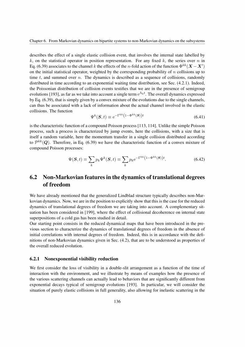
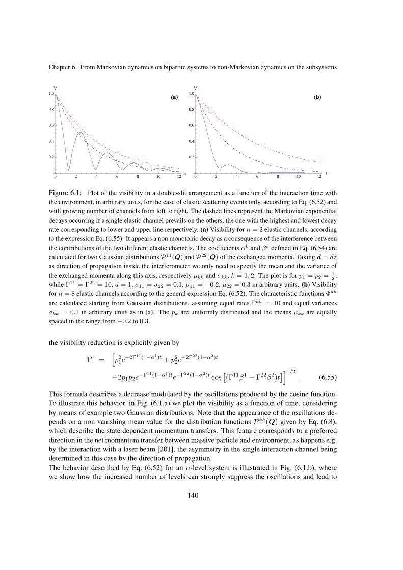
6.2 Non-Markovian features in the dynamics of translational degrees of freedom . . . 1366.2.1 Nonexponential visibility reduction . . . . . . . . . . . . . . . . . . . . 1366.2.2 Back flow of information . . . . . . . . . . . . . . . . . . . . . . . . . . 141

7 Conclusions 145

A Quantum measurement 149

viii

Contents

B One-parameter semigroups 153

C Trace distance 155

D General bound and non-convexity for correlations 159

E Measure of non-Markovianity 161

F Fourth order time-convolutionless master equation for the damped two-level system 165

Bibliography 169

ix

Chapter 1

Introduction

The standard textbook presentation of quantum mechanics deals with closed quantum systems,whose evolution is described by means of a one-parameter group of unitary operators generatedby a self-adjoint Hamiltonian. In the last few decades, an increasing effort has been put into de-veloping the theory of open quantum systems [1], that is quantum systems in interaction with anenvironment. The reasons for this growing interest can be traced back to practical as well as fun-damental questions.Every concrete physical system is unavoidably affected by the interaction with an environment.Indeed, this is quite a generic statement, that can be applied to classical physics, as well. Thecrucial point is that the interaction of a quantum system with an environment strongly influencesthose features that cannot be enclosed into a classical description of the system. One of the mostrepresentative examples is given by the phenomenon that goes under the name of decoherence [2].A quantum system interacting with an environment loses, typically on a very short time scale, thecapability to exhibit superpositions among states belonging to a certain basis, ultimately depend-ing on the specific form of the interaction between the open system and the environment. Thus,the study of open quantum systems has become of great relevance in all those areas of physicswhere the quantum nature of concrete physical systems in contact with an environment is takeninto account, representing a basic resource. By way of example, one only needs to think of quan-tum information [3] as well as quantum optics [4].As well known, quantum mechanics is an essentially statistical theory, meaning that all its predic-tions have a statistical character. The more recent statistical formulation of quantum mechanics,originated from the work by Ludwig [5, 6], Holevo [7] and Kraus [8], is based on the idea thatquantum mechanics is a probability theory, significantly different from the classical one, ratherthan an extension of classical mechanics. The reproducible quantities of the theory are the rel-ative frequencies according to which a large collection of identically prepared quantum systemstriggers proper measurement apparata. Indeed, a quantum system subjected to a coupling with ameasurement apparatus represents an open system interacting with a macroscopic environment.The foundations of quantum mechanics are then deeply connected to the theory of open quantumsystems through the notion of measurement process. Thus, it should not be surprising that manyconcepts and tools introduced within the statistical formulation of quantum mechanics are now at

1

Chapter 1. Introduction

the basis of the description of open quantum systems.Moreover, the progressive loss of typical quantum features as a consequence of the interaction withan environment is commonly seen as a crucial step in the direction of a reconciliation between thequantum and the classical characterization of physical systems, since it provides a quantitative ex-planation of the absence of quantum effects above a certain size scale. Nevertheless, it should bekept in mind that the loss of quantum coherence for a microscopic system interacting with somemacroscopic system is not the same as the classical behavior that macroscopic systems themselvesactually exhibit. The latter, in fact, allows an objective description that cannot be explained simplyin terms of decoherence [9, 10]. A more suitable characterization of macroscopic systems shouldthen be taken into account. One of the possibilities is to base the description of macroscopic sys-tems on quantum statistical mechanics, extended to non-equilibrium situations. This could lead tothe appearance of an objective classical behavior for a proper subset of physical quantities, possi-bly yielding a unified description of microscopic and macroscopic systems [11, 12, 13].

By moving aside from the well-established field of closed quantum systems, where the unitarytime evolution is directly fixed by the corresponding Hamiltonian operator, the description of thedynamics of quantum systems gets immediately more involved. Which are the most general equa-tions of motion that provide a well-defined time evolution? How are these equations connectedto the underlying microscopic description of the interaction between the open system and theenvironment? Is it possible to identify different classes of open-system dynamics on the basisof some physically as well as mathematically motivated criterion? What are the proper ways toquantitatively characterize the dynamics of open quantum systems under completely generic ini-tial conditions? All these very basic questions are still at the moment only partially answered.A result of paramount importance has been obtained by characterizing the class of dynamics de-scribed by completely positive quantum dynamical semigroups. The expression of the generatorsof such semigroups, that determines the equation of motion for the open system, has been fullyidentified [14, 15], providing a reference structure often called Lindblad equation. This class ofdynamics is usually considered the quantum counterpart of classical homogeneous Markov pro-cesses. The main physical idea behind this correspondence is that in both cases the memory effectsare negligible. In order to describe the dynamics of an open quantum system by disregarding atany time the influence of the previous interaction with the environment, one typically assumesthat the characteristic time scale of the environment is much shorter than that of the open sys-tem. Indeed, there are many concrete physical systems where this condition is not satisfied, sothat one has to look for a more general description of the dynamics. Just to mention an example,the development of technologies that access time-scales of the order of femtoseconds allows toobserve phenomena in which non-Markovian features of the dynamics unavoidably play a funda-mental role [16, 17]. As a consequence, in recent years a lot of research work has been devotedto quantum dynamics beyond the Markovian description. Apart from the explicit detailed treat-ment of many specific quantum systems where memory effects show up and the characterizationof general classes of non-Markovian dynamics, efforts have been made to actually define what ismeant by a non-Markovian quantum dynamics and to quantify the degree of non-Markovianity ofa given quantum dynamics [18, 19, 20]. One of the main focuses of the present Thesis is preciselyto investigate the very definition of non-Markovian quantum dynamics, with a particular emphasis

2

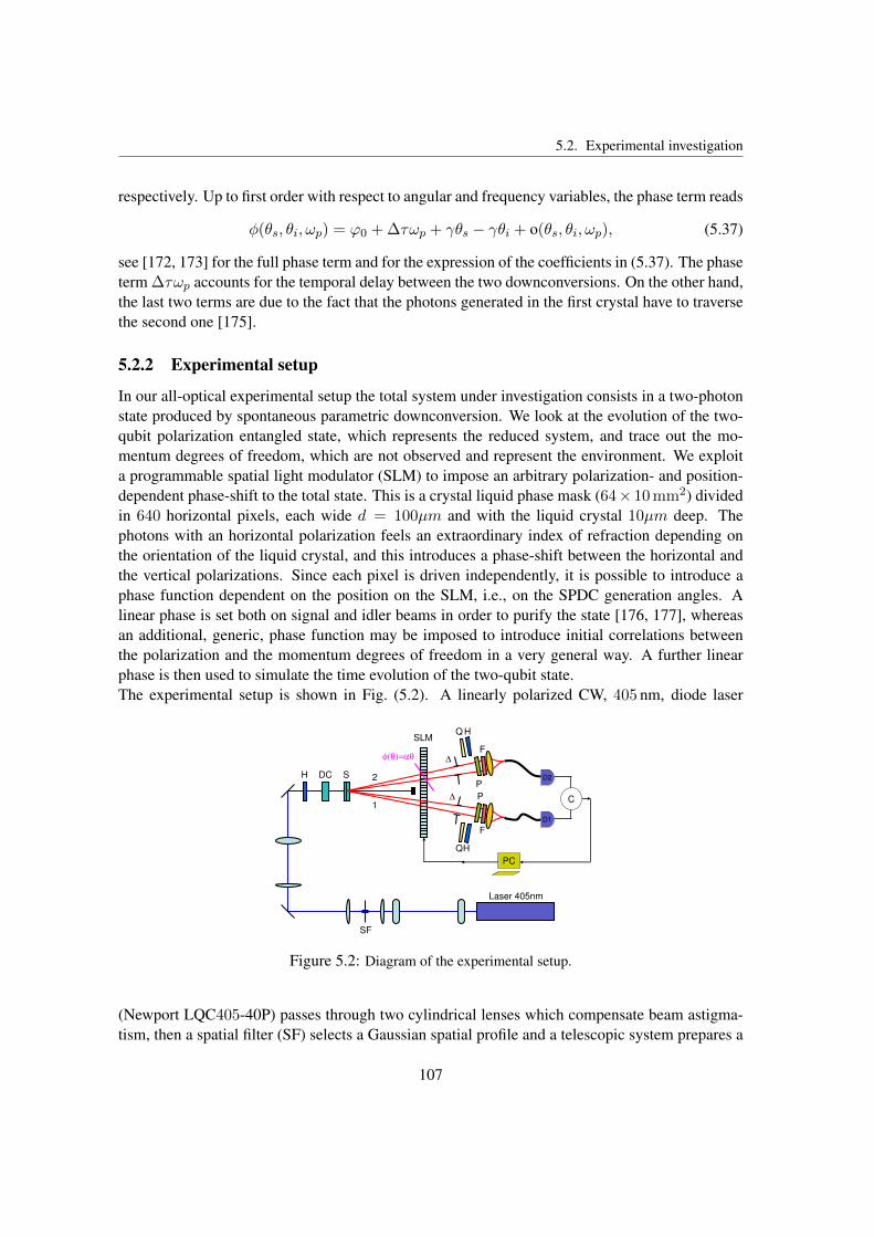
on its relations to the classical notion of non-Markovianity. The entire analysis is performed bymeans of two different ways to characterize the dynamics of open quantum systems. The first isbased on the use of suitable evolution maps, often referred to as quantum dynamical maps [1],defined on the state space of the open system. The connections with the corresponding equa-tions of motion are investigated, as well. The second approach has been introduced very recently[19, 21] and it relies on the idea that the dynamics of open systems can be described in terms ofthe information flow between the open system and the environment in the course of the dynamics.Such an information flow is quantitatively defined by means of trace distance, that measures thedistinguishability between quantum states [3]. In particular, the dynamics of an open system ischaracterized by monitoring the evolution of the trace distance between couples of states of theopen system that evolve from different initial total state.The interaction between an open quantum system and an environment naturally induces correla-tions among these two systems. Nevertheless, it is usually assumed that the open system and theenvironment are uncorrelated at the initial time, thus assigning a very special status to the instant oftime where one starts to monitor the evolution of the open system. From a physical point of view,this is not always justified, especially outside the weak coupling regime [22, 23, 24]. It is then ofinterest to extend the different approaches to open-system dynamics in order to include possibleinitial correlations. With respect to this, the definition of dynamical maps can become problem-atic. In fact, in the presence of initial system-environment correlations, contrary to the case of anuncorrelated initial state, there is not a unique way to define dynamical maps on the state space ofthe open system and their physical meaning can be established only inside proper domains, thatare not easy to detect in an explicit way [25]. Furthermore, these maps turn out to depend onquantities related to the global system that cannot be generally accessed on concrete experimentalsituations. In this Thesis, the quantitative characterization of the open-system dynamics with ini-tial correlations is presented from a different point of view [26]. Namely, this is based on the sameapproach previously mentioned in connection with the definition of non-Markovianity in quantumdynamics, relying on the analysis of trace-distance evolution as a consequence of an informationflow between the open system and the environment. One of the main advantages of studying thedynamics of open quantum systems by means of trace distance consists in its clear and unambigu-ous experimental meaning, due to the fact that it only requires to perform measurements on theopen system, without the need of any information about the total system or the structure of theinteraction between the system and the environment. The first experimental investigation of thedynamics of an open quantum system in the presence of initial correlations with the environmenthas been recently achieved by the quantum optics group at the University of Milan [27].

Outline

This Thesis is organized as follows.In Chapter 2, we introduce the basic concepts and tools used in the statistical formulation of quan-tum mechanics that will be at the basis of the entire subsequent analysis. In particular, we focus ontransformation maps of quantum states, consisting in completely positive trace preserving linearmaps. We first present such maps, as well as their properties and representations, in an abstract

3

Chapter 1. Introduction

way, while at the end of the chapter we show how they naturally provide a description of thedynamics of open quantum systems, if the open system and the environment are initially uncorre-lated.Chapter 3 concerns the equations of motion that can be associated with the evolution maps previ-ously introduced and that are usually referred to as quantum master equations. We show to whatextent the dynamics of open quantum systems can be described by both local and non-local intime master equations, also presenting some general methods to pass from one kind of equationto the other. This analysis is then applied to a two-level system interacting via Jaynes-CummingsHamiltonian with the radiation field. We focus on the differences between the operator structure oflocal and non-local master equations, that generally depend on the initial state of the environment.Moreover, we face the problem of characterizing those equations of motion that guarantee a well-defined time evolution. After recalling basic results related to quantum dynamical semigroups andin particular the Lindblad equation, we present a local as well as a non-local generalization.In Chapter 4, we discuss the conceptually different definitions used for the non-Markovianity ofclassical processes and quantum dynamics. We first deal with classical stochastic processes, fo-cusing in particular, by means of a class of non-Markov processes, on the difference between theconcepts of conditional probability and transition map. This clearly demonstrates that the Marko-vianity or non-Markovianity of a classical stochastic process cannot be accessed by the evolutionof its one-point probability distribution only. We further show how recently introduced criteria forthe non-Markovianity of quantum dynamics naturally induce analogous criteria on the dynamicsof a classical one-point probability distribution. These are sufficient, but not necessary conditionsfor a classical stochastic process to be non-Markovian. The first criterion [19] is based on the anal-ysis of the information flow between the open system and the environment, performed by meansof the trace distance between pairs of open-system states. The second [20] is instead defined interms of divisibility properties of the dynamical maps. The comparison between these two criteriaand the related quantifiers of non-Markovianity is then performed in the quantum setting. Here,we take advantage of the definition of a class of non-Markovian quantum dynamics with a clearphysical meaning as well as a direct connection with classical stochastic processes.In Chapter 5, we deal with the dynamics of open quantum systems in the presence of initial system-environment correlations. We first briefly recall how the approach based on quantum dynamicalmaps can be applied to this situation, then we present a further generalization of the Lindbladequation, consisting in a system of homogeneous equations for proper dynamical variables. Therest of the chapter is focused on the different description of reduced dynamics with initial correla-tions, which is given in terms of trace-distance evolution. We first present the general theoreticalscheme, and then we report its first experimental realization [27] through an all-optical apparatus,in which the dynamics of couples of entangled photons generated by spontaneous parametric downconversion has been investigated. Finally, we take once again the Jaynes-Cummings Hamiltonianinto account, but now allowing for a fully generic initial total state. The trace-distance evolution ofthe open-system states evolving from the thermal state and its corresponding uncorrelated productstate elucidates how the open system dynamically uncovers typical features of the initial correla-tions.In Chapter 6, we consider a physical system associated with an infinite dimensional Hilbert spaceand we discuss its decoherence and non-Markovianity. Namely, we describe the dynamics of a

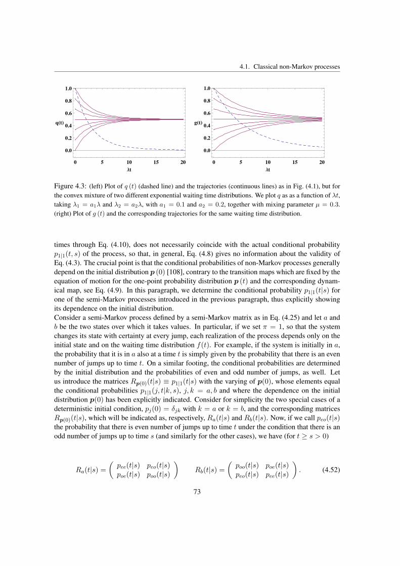
4

massive test particle with translational and internal degrees of freedom that interacts through col-lisions with a background low density gas. This is a representative model for the description ofcollisional decoherence. Under suitable approximations, the evolution of the massive particle canbe characterized by a semigroup evolution. Nevertheless, there are situations where it is usefulto focus on the dynamics of translational degrees of freedom alone, considering the internal de-grees of freedom as part of the environment. A typical example is when the internal state of themassive particle is not resolved in visibility measurements. The resulting dynamics for the trans-lational degrees of freedom can be given in terms of the generalization of the Lindblad equationintroduced in Chapter 5, that allows to include initial system-environment correlations as well asnon-Markovian effects. The latter are explicitly described by taking into account the evolution ofboth interferometric visibility and trace distance, which are shown to be strongly related for themodel at hand.This Thesis is built upon the material contained in [28, 29, 30, 31, 27] , as will be indicated in thevarious chapters more precisely.

5

Chapter 2

Quantum dynamical maps

This chapter provides a short introduction to basic concepts of quantum mechanics which will beemployed throughout the entire Thesis. As stated in the Introduction, the quantum descriptionof physical systems will be presented according to the statistical formulation of quantum me-chanics. This approach turned out to be very useful for the characterization of quantum systems,closed as well as open, leading to the introduction of new concepts and tools which allowed adeeper understanding of the quantum description of reality, both from theoretical and experimen-tal points of view. For more rigorous and detailed presentations of this topic the reader is referredto [32, 33, 1, 34, 13, 35], in addition to the works by Ludwig [5, 6], Holevo [7] and Kraus [8]already mentioned in the Introduction.In quantum mechanics experiments are by necessity of statistical nature. The most simple setupcan be typically described as a suitably devised macroscopic apparatus preparing the microscopicalsystem one wants to study, that in turn triggers another macroscopic device designed to measurethe value of a definite quantity. The predictions of the theory must be related to a large collec-tion, or ensemble, of identically prepared quantum systems. The experimental quantity that hasto be compared with the theory is the relative frequency according to which the elements of theensemble trigger the registration apparatus. According to this picture, the states of the systemare associated with preparation procedures, while the observables are associated with registrationprocedures.Spaces of operators on Hilbert spaces are the natural mathematical framework where states as wellas observables of physical systems are represented. Consequently, the evolution of a quantum sys-tem is characterized by means of maps taking values in these operator spaces. This applies totransformations due to a measurement performed on the system, as well as to dynamical evolu-tions. Indeed, the dynamics of closed systems is described by a very special kind of these maps;namely, unitary time evolutions that are uniquely fixed by a self-adjoint operator. Before focusingon the description of the dynamics of open quantum systems in the next chapters, we introducehere the general setting. The transformations of quantum states due to measurement processes canbe described in terms of the so-called instruments, as briefly recalled in Appendix A.In the first section, we present the mathematical objects representing the states as well as the ob-servables of a quantum system. The set of quantum states of a physical system associated with

7

Chapter 2. Quantum dynamical maps

an Hilbert space H is identified with the set of statistical operators on H, while the definitionof observable as positive operator-valued measure (POVM) consists in a map with values in theBanach space of bounded operators on H. We first introduce the relevant sets of linear operatorson H, therefore connecting them to the statistical formulation of quantum mechanics. After that,we introduce the quantum description of composite systems and in particular the different kindsof preparation procedures that characterize product states, separable states and entangled states ofa bipartite system. The notion of quantum discord is briefly presented, as well. We also introducethe concepts of partial trace and marginal states of a bipartite state, since they play a basic role inthe theory of open quantum systems.In the second section, we characterize the maps representing transformations of quantum states.This is firstly accomplished in an abstract way, by defining the space of linear maps on the operatorspaces introduced in the first section. We describe different ways in order to represent these maps,thus introducing in a compact and unified way several techniques which are regularly used in thetheory of open quantum systems. After that, we discuss general properties satisfied by those linearmaps that properly describe transformations of quantum states, focusing on complete positivity.Finally, in the last part of the chapter, we introduce the concept of reduced dynamics, which pro-vides a description of the evolution of an open quantum system interacting with an environment.We see how, under the hypothesis of an initial product state, this consists in a family of completelypositive trace preserving linear maps.

2.1 Basic concepts

2.1.1 Relevant operator spaces

In quantum mechanics each physical system is associated with a separable Hilbert space H; wewill denote its scalar product as 〈ϕ|ψ〉 and the induced norm as ‖ψ‖ =

√〈ψ|ψ〉, with |ψ〉, |ϕ〉 ∈

H. Let T (H) be the set of linear trace class operators on H. A linear operator σ on H belongs tothe set T (H) if

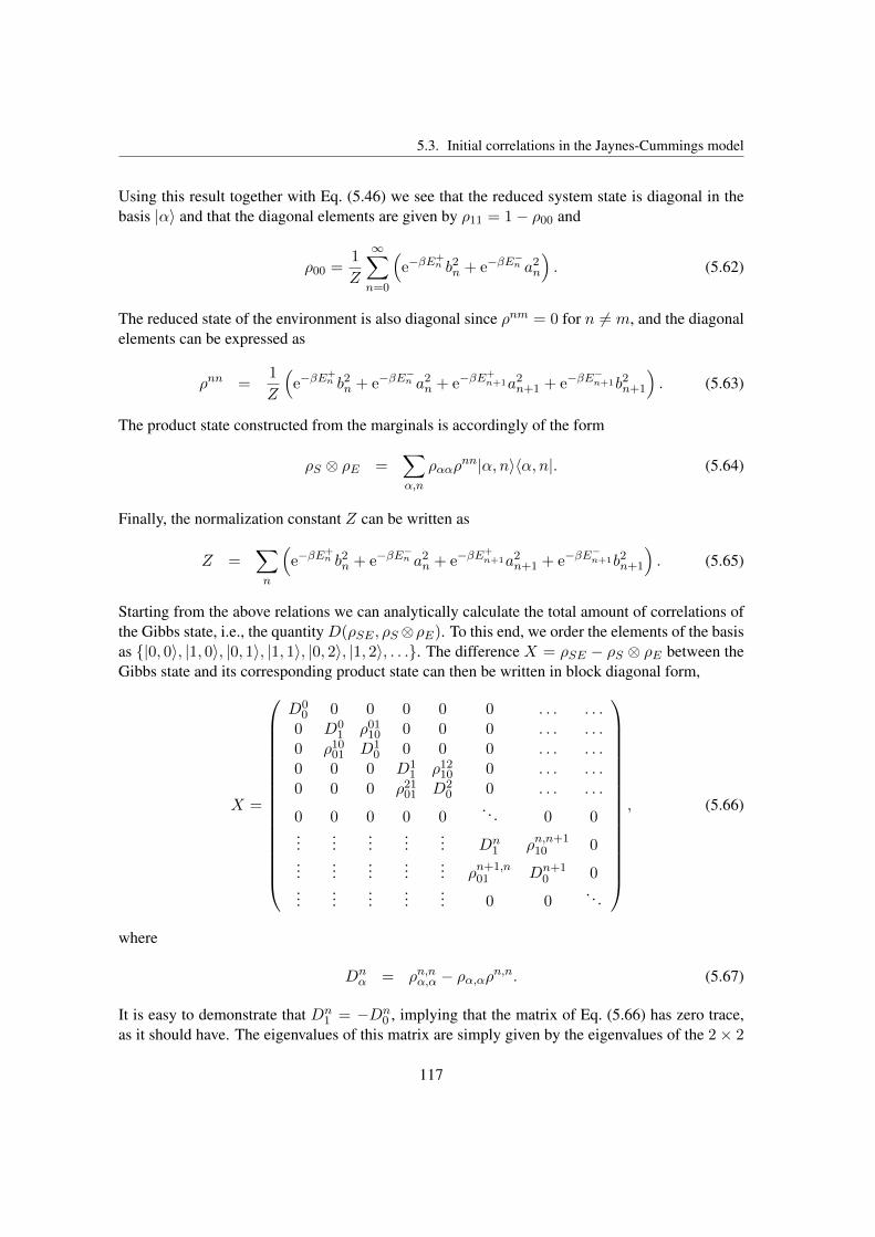
Tr[√σ†σ] <∞. (2.1)

The trace of an operator σ is defined as

Tr[σ] =∑k

〈uk|σ|uk〉, (2.2)

with |uk〉k=1,2,... orthonormal basis in H. The series in Eq. (2.2) does not depend on the basisand for σ ∈ T (H) it is absolutely convergent. The set T (H) is a Banach space with norm ‖ · ‖1,which is called trace norm, defined by

‖σ‖1 = Tr[|σ|] = Tr[√σ†σ] σ ∈ T (H). (2.3)

In addition to its central role in the definition of the set of quantum states, the trace norm canbe directly exploited in order to characterize the dynamics of open quantum systems, as will beshown in Chapters 4 and 5.

8

2.1. Basic concepts

The set S(H) of statistical operators onH is given by the set of linear, semi-positive definite andwith unit trace operators onH,

S(H) = ρ ∈ T (H)|ρ ≥ 0, ‖ρ‖1 = 1 , (2.4)

where a semi-positive1 definite operator ρ ≥ 0 on an Hilbert space H is a self-adjoint operatorsuch that

〈ψ|ρ|ψ〉 ≥ 0 ∀ |ψ〉 ∈ H. (2.5)

Note that for any σ ∈ T (H) one has Tr[σ] = ‖σ‖1 if and only if σ is positive definite and that theset of self-adjoint operators in T (H) is the smallest linear space containing S(H). The set S(H)is convex, so that

ρk ∈ S(H), λk ≥ 0∑k

λk = 1⇒∑k

λkρk ∈ S(H). (2.6)

One dimensional projectors are the extremal points of this set, that is the elements that do notadmit any further demixture: if ρ = |ψ〉〈ψ| with ‖ψ‖ =

√〈ψ|ψ〉 = 1, then

ρ = λρ1 + (1− λ)ρ2 0 < λ < 1 ρ1, ρ2 ∈ S(H)⇒ ρ = ρ1 = ρ2. (2.7)

The dual space to T (H) consists of all the linear bounded operators on H and will be denoted asB(H). This is a Banach space with norm ‖ · ‖∞ defined through

‖A‖∞ = sup‖ψ‖=1

‖A|ψ〉‖, (2.8)

with |ψ〉 ∈ H and A ∈ B(H). The form of duality between B(H) and T (H) is given by the trace:

Tr : B(H)× T (H) → C;

(A, σ) → Tr[A†σ]. (2.9)

The trace in Eq. (2.9) is well defined since the product of a bounded operator and a trace classoperator is a trace class operator [36]. Moreover, it holds the relation

|Tr[Aσ]| ≤ ‖A‖∞‖σ‖1. (2.10)

Finally, let us introduce the set of Hilbert-Schmidt operators onH, which will be denoted asD(H),i.e. the set of linear operators X onH such that

Tr[X†X] <∞. (2.11)

The set D(H) is a Banach space with norm ‖ · ‖2 defined by

‖X‖2 =√

Tr[X†X] X ∈ D(H). (2.12)

1From now on, we will use the more common expression positive definite operator.

9


Since for every linear operator A onH it holds

‖A‖∞ ≤ ‖A‖2 ≤ ‖A‖1, (2.13)

one has T (H) ⊂ D(H) ⊂ B(H). The duality relation in Eq. (2.9) induces a scalar product onT (H) as well as on D(H), the Hilbert-Schmidt scalar product:

〈σ, σ〉 = Tr[σ†σ], (2.14)

with σ, σ ∈ T (H) or σ, σ ∈ D(H); note that this scalar product is well-defined also on D(H)since the product of two Hilbert-Schmidt operators is a trace class operator. Indeed, T (H) is notgenerally an Hilbert space, while D(H) is an Hilbert space with respect to the scalar product de-fined in Eq. (2.14), since it is a Banach space with respect to the corresponding induced norm, seeEq. (2.12).

2.1.2 Statistical formulation of quantum mechanics

The set of statistical operators S(H) represents the set of quantum states of the physical systemassociated with the Hilbert space H [37]. According to the statistical formulation of quantummechanics, a statistical operator ρ provides a complete characterization of an ensemble of quantumsystems prepared in a specific way, typically by a suitably devised macroscopic apparatus. The setS(H) is convex and one dimensional projectors are its extremal points, referred to as pure states,see Eqs. (2.6) and (2.7). On the other hand, a state ρ which is not pure, a mixed state, in generaladmits infinitely many ways to be written as a convex combination of other states. Among thedifferent decompositions, every statistical operator ρ can be expressed as a convex combination ofpure orthogonal states. Since a generic statistical operator ρ has a point spectrum of eigenvaluesλk ≥ 0 and 0 is the only possible accumulation point 2, one can always write

ρ =∑k

λk|ψk〉〈ψk| λk ≥ 0∑k

λk = 1; 〈ψk′ |ψk〉 = δk,k′ , (2.15)

with pk and |ψk〉, respectively, eigenvalues and eigenvectors of ρ.As already mentioned in the introduction to this chapter, observables are instead associated withregistration procedures. Their mathematical representatives consist in positive operator-valuedmeasures (POVMs), which are maps with values in the set of bounded operators. Let Ω be theset of the possible outcomes of a measurement performed on a given observable and let A(Ω) bea σ-algebra over Ω. A POVM F is a map associating to each element M ∈ A(Ω), a boundedoperator F (M) ∈ B(H), called effect, i.e.,

F (·) : A(Ω) → B(H)

M → F (M), (2.16)

2This is a consequence of the general theory on compact self-adjoint operators on Hilbert spaces (every trace classoperator is compact [36]): the nonzero eigenvalues have finite dimensional eigenspaces and, in the case of an infinitedimensional Hilbert space, the sequence of eigenvalues converges to 0.

10

2.1. Basic concepts

in a way such that

0 ≤ F (M) ≤ 1

F (∅) = 0 F (Ω) = 1

F (∪iMi) =∑i

F (Mi) if Mi ∩Mj = ∅ for i 6= j. (2.17)

Note that the effect F (M) is not necessarily a projection operator, since the idempotence relationF 2(M) = F (M) is not requested. If this further condition holds for all M ∈ A(Ω) one has aprojection-valued measure (PVM). The spectral theorem establishes a one-to-one correspondencebetween the set of PVMs and the set of self-adjoint operators on H, so that one can recover thestandard definition of observable as self-adjoint operator.The duality relation expressed by Eq. (2.9) provides the statistical formula allowing to compare thetheory with the experiment: given a system prepared in the state ρ, the probability that a quantitydescribed by the POVM F takes value in M is

µFρ (M) = Tr[ρF (M)]. (2.18)

Note that the properties of trace class operators and POVMs ensure that µFρ (M) is a numberbetween 0 and 1 and that the map

µFρ (·) : A(Ω) → [0, 1];

M → µFρ (M) = Tr[ρF (M)] (2.19)

is a classical probability measure. The crucial difference with respect to classical probability the-ory is that there is not a common probability density allowing to express the probability measuresof all the observables.The basic relation in Eq. (2.18) enables the following interpretation to the possibly infinite ways towrite a mixed state as a convex combination of other states. The different demixtures do generallycorrespond to preparation procedures performed with different devices and which are incompati-ble, in the sense that they cannot be accomplished together, but which lead to the same statisticsin any subsequent experiment, thus being physically indistinguishable. In fact, since they are allrepresented by the same state ρ, the probabilities they assign to the different observables accord-ing to Eq.(2.18) are the same. Thus, more precisely, a statistical operator ρ is to be understoodas the mathematical representative of an equivalence class of preparation procedures. To give anexample, the spectral decomposition in Eq. (2.15) indicates that an ensemble made of a large num-ber, let us say n, of quantum systems has been prepared from the mixture of different ensemblesof identically prepared quantum systems, each of these ensembles with nk = pkn elements anddescribed by the pure state |ψk〉.In an analogous way, according to the statistical formulation of quantum mechanics, an observableis to be understood as the mathematical representative of an equivalence class of registration pro-cedures. In fact, different and generally incompatible macroscopic devices can be used to measurethe same physical quantity. From a mathematical point of view, this is connected to the possibilityof introducing different instruments for the same POVM, see Appendix A.

11


Finally, note that by means of Eq. (2.18) and the spectral theorem, one gets the usual formulafor the mean value 〈H〉 of an observable represented by a self-adjoint operator H , given that thesystem is in the state ρ:

〈H〉 = Tr[ρH]. (2.20)

2.1.3 Composite quantum systems and correlations in quantum states

The notion of composite quantum system stands at the very foundation of the theory of openquantum systems. Indeed, an open system and the corresponding environment are the two parts ofa composite system. Then, it is worth recalling here the main features of the quantum descriptionof composite systems.Consider two physical systems associated withH1 andH2, respectively, and representing the twoparts of a composite system. The Hilbert space associated with the total system composed by thetwo subsystems is given by the tensor productH = H1⊗H2. Fixed two orthonormal bases |ψj〉and |ϕk〉 inH1 andH2, respectively, a generic element ofH may be written as

|ψ〉 =∑jk

cjk |ψj〉 ⊗ |ϕk〉, (2.21)

so that the set |ψj〉 ⊗ |ϕk〉 is a basis in the tensor product Hilbert spaceH. On the same footing,given two linear operators, ω on H1 and χ on H2, one can define their tensor product ω ⊗ χ bymeans of the relation

(ω ⊗ χ) (|ψ〉 ⊗ |ϕ〉) = ω|ψ〉 ⊗ χ|ϕ〉, (2.22)

and then by linear extension on the wholeH. Any operator O onH can be written as

O =∑k

ωk ⊗ χk. (2.23)

The set of states of the composite system is S(H1 ⊗H2). The simplest example of such a state isgiven by the product state

% = ρ⊗ σ, (2.24)

with ρ ∈ S(H1) and σ ∈ S(H2), physically representing two uncorrelated subsystems. Thismeans that a product state can be prepared by acting locally and in a fully independent way on thedifferent parts of the composite system. If also the registration procedure is performed indepen-dently on the two subsystems, so that it is described by effects of the formA⊗B, the probabilitieson the two subsystems factorize since, see Eq. (2.18),

Tr[ % (A⊗B)] = Tr[ (ρ⊗ σ) (A⊗B)] = Tr[ ρA]Tr[σ B]. (2.25)

This is simply the case of two independent experiments performed at the same time on the twosubsystems.A more involved situation occurs if the preparation procedure consists in local operations per-formed on the two subsystems plus a classical communication between them, so that one intro-duces correlations between the two parts in a classical way. The states which are prepared in this

12

2.1. Basic concepts

way can be represented by statistical operators of the form [38]

% =d∑

k=1

pk ρk ⊗ σk pk > 0∑k

pk = 1, (2.26)

where ρk ∈ S(H1), σk ∈ S(H2) and d < ∞. In particular, a state % on a bipartite Hilbert spaceH = H1 ⊗ H2 is called separable if and only if it can neither be represented nor approximatedas in Eq. (2.26). The states which are not separable are called entangled. Entanglement is adistinctive feature of quantum mechanics [39, 40], playing a central role in the foundations ofquantum mechanics, as well as being a key resource for quantum-information sciences. A lotof questions connected to entanglement are still open and highly debated, e.g. the problem ofestablishing whether an assigned state % can be written in the form as in Eq. (2.26) or how toquantify entanglement, but they go beyond the scope of this work (for a review about entanglementand its applications to quantum communication see [41]). However, it is worth recalling here thatthe characterization of entanglement can be fully accomplished in the case of pure states3. Forany pure state |φ〉 on a bipartite Hilbert space there exist orthonormal bases, the Schmidt bases,|χ1,k〉 and |χ2,k〉 in H1 and H2, respectively, such that |φ〉 can be written according to theSchmidt decomposition [3]

|φ〉 =N∑k=1

√pk |χ1,k〉 ⊗ |χ2,k〉 pk > 0

∑k

pk = 1, (2.27)

where N is the minimum between the dimensions of H1 and H2. The Schmidt rank, i.e. thenumber of non-zero Schmidt coefficients

√pk, is invariant with respect to unitary transformations

of the form U ⊗ V and then it does not depend on the particular Schmidt bases chosen, but it isuniquely associated with the given state |φ〉. A pure bipartite state |φ〉 is entangled if and only ifit cannot be written as a product state |ψ〉 ⊗ |ϕ〉 and then if and only if its Schmidt rank is higherthan 1. On the other hand, given a finite N in Eq. (2.27), a state is said to be maximally entangledif its Schmidt coefficients are all equal to N−1/2, i.e. if it is of the form

|φ〉ME =1√N

N∑k=1

|χ1,k〉 ⊗ |χ2,k〉. (2.28)

The definition of entangled states, which distinguishes classical from quantum correlations on thebasis of different kinds of preparation procedures, has been recently refined by the introduction ofthe notion of quantum discord [42, 43], which is instead focused on the effects of local measure-ment performed on the system. Namely, a state has a vanishing quantum discord if there existsa local basis for one of the subsystems in which the observer can perform measurements with-out modifying the state. The latter condition is a general property of classical systems, but it isnot usually satisfied in quantum mechanics, which motivates the definition. Quantum discord is

3At least in the bipartite case; one can see the above mentioned reference also for a discussion of multipartiteentanglement, i.e. the entanglement related to composite quantum systems with more than two parts, associated withHilbert spaces of the formH1 ⊗H2 ⊗ . . .⊗Hn.

13


asymmetric under the change of the two subsystems. In particular, if the local measurements areperformed on the first subsystem, a state with zero discord is of the form

% =∑k

pk|vk〉〈vk| ⊗ σk, (2.29)

with 0 ≤ pk ≤ 1,∑

k pk = 1, |vk〉k=1,2,... a basis in H1 and σk statistical operators on H2.In fact, one can see [43] that a state % can be written as in Eq. (2.29) if and only if it satisfies thefollowing invariance:

% =∑k

Πk%Πk, (2.30)

with Πk = |vk〉〈vk| ⊗ 1 rank-one projectors acting in a non-trivial way on the first subsystem.Thus, according to (A.12), a zero-discord state is not modified by a non-selective measurement ofan observable of the first subsystem associated with the non-degenerate self-adjoint operator witheigenvectors |vk〉k=1,2,.... Indeed, a similar analysis can be done for states that have vanishingdiscord with respect to the second subsystem, and a symmetrized version of quantum discord canbe introduced, thus allowing for the generalization to multipartite scenario [44]. As it clearlyappears from Eqs. (2.26) and (2.29), states with vanishing discord form a subset of separablestates and there are separable states with nonzero discord. It has been shown [45] that the set ofzero-discord states has measure zero.

Partial trace

If one is only interested in observables related to one subsystem, that is only in operators of theform A ⊗ 1 (or, equivalently, 1 ⊗ B), it is convenient to introduce the statistical operator, whichis referred only to the subsystem of interest, defined by taking the partial trace of the total state %:

ρ1 ≡ tr2%, (2.31)

where ρ1 ∈ S(H1) since % ∈ S(H1 ⊗H2) and tr2 indicates the partial trace performed over thesecond Hilbert space. Given a basis |uk〉 inH2 and |ψ〉, |ζ〉 ∈ H1, the partial trace in Eq. (2.31)means that

〈ψ|ρ1|ζ〉 = 〈ψ|tr2%|ζ〉 =∑k

(〈uk| ⊗ 〈ψ|) % (|uk〉 ⊗ |ζ〉) . (2.32)

A completely specular relation holds for the state ρ2 = tr1% ∈ S(H2). The two states ρ1 and ρ2

are often called marginal states with respect to the total state %. From Eq. (2.32) it is in fact clearthe analogy with the classical marginal probability distributions obtained from a joint probabilitydistribution. From a physical point of view, the partial trace tr2 describes the average performedover the degrees of freedom of the system associated with H2. The statistical operator defined inEq. (2.31) allows to describe the whole statistic of the first subsystem: given an effect of the formA⊗ 1, the probability associated with it by means of Eq. (2.18) can be calculated as

Tr[%(A⊗ 1)] = tr1[ρ1A]. (2.33)

14

2.2. States transformations and complete positivity

It can be shown [3] that the partial trace is the unique function f : S(H1 ⊗ H2) → S(H1) suchthat tr1[ f(%)A] = Tr[%(A⊗ 1)] for any % ∈ S(H) and A ∈ B(H), so that this way of describingthe state of subsystems is the only compatible with the statistical formulation presented in theprevious paragraph.As a first application of the partial trace, one can immediately see that the Schmidt decompositionof a pure bipartite state, see Eq. (2.27), yields

ρ1 = tr2[|φ〉〈φ|] =∑k

pk|χ1,k〉〈χ1,k|

ρ2 = tr1[|φ〉〈φ|] =∑k

pk|χ2,k〉〈χ2,k|, (2.34)

so that the marginal states of a pure bipartite state have the same eigenvalues. Furthermore, bymeans of the Schmidt decomposition, one can see that if at least one of the marginal states is pure,then the total state % has to be a product state, that is

ρ1 = tr2[%] = |ψ〉〈ψ| or ρ2 = tr1[%] = |ϕ〉〈ϕ| =⇒ % = ρ1 ⊗ ρ2, (2.35)

with |ψ〉 ∈ H1 and |ϕ〉 ∈ H2, for a proof see [46]. Finally, note that the set of states in S(H1⊗H2)which have the same marginals ρ1 and ρ2 is a convex set. This set of course includes the productstate obtained from the marginals of %, i.e.

ρ1 ⊗ ρ2 ρ1 = tr2[%] ρ2 = tr1[%]. (2.36)

This kind of states can be used in order to study the dynamics of open quantum systems in thepresence of initial correlations between the open system and the environment, as will be shown inChapter 5.

2.2 States transformations and complete positivity

2.2.1 Linear maps on operator spaces

Let us now consider the mathematical representatives of transformations of quantum states, thatis, linear maps on the previously introduced operator spaces. First, we are going to describe onestep transformations without directly connecting them to any specific evolution process. In thisand in the next two paragraphs we describe in an abstract way how to represent a linear map andwhen it properly describes a transformation of quantum states. The connection with the dynamicsof open quantum systems will be given in the last paragraph of the section. The connection withmeasurement processes on quantum systems is briefly presented in Appendix A. For simplicity,we are moving to the finite-dimensional case, i.e. we are assuming H = CN . All the linear oper-ators on finite-dimensional Hilbert spaces are bounded, so that the three Banach spaces presentedin the previous section coincide with the space of linear operators on CN , which will be denotedas L(CN ).

15


Consider the Banach space4 L(CN ) of linear operators on the finite-dimensional Hilbert spaceH = CN . Note thatL(CN ) equipped with the Hilbert-Schmidt scalar product defined in Eq. (2.14)is an Hilbert space. Every linear map Λ on L(CN ) is thus a linear operator on an Hilbert space.As such, we will say that a linear map Λ is a self-adjoint operator on L(CN ) if it equals its adjointoperator Λ†, defined through

〈Λ†(χ), ω〉 = 〈χ,Λ(ω)〉 ∀χ, ω ∈ L(CN ), (2.37)

where 〈χ, ω〉 indicates the Hilbert-Schmidt scalar product between χ and ω, see Eq. (2.14). Fur-thermore, we will say that a self-adjoint operator Λ is positive definite if it satisfies the conditionexpressed in Eq. (2.5); explicitly,

〈ω,Λ(ω)〉 ≥ 0 ∀ω ∈ L(CN ). (2.38)

Note that we have taken advantage of the fact that L(CN ) is a finite-dimensional Hilbert space.More in general, considering a linear operator Λ acting on the set T (H) of trace class operatorson the infinite-dimensional Hilbert spaceH, one would instead introduce the concept of dual mapon the space B(H), dual to T (H). The map Λ∗ dual to Λ is defined as

(Λ∗(A), σ) = (A,Λ(σ)) A ∈ B(H) σ ∈ T (H), (2.39)

where (A, σ) = Tr[A†σ] indicates the duality relation between B(H) and T (H), see Eq. (2.9).In the case of a finite dimensional Hilbert space H the definition of dual map reduces to that ofadjoint operator in Eq. (2.37).Let σαα=1,...,N2 be a basis in L(CN ), orthonormal with respect to the Hilbert-Schmidt scalarproduct:

〈σβ, σα〉 = Tr [σ†β σα] = δαβ. (2.40)

Then, every linear operator Λ on the Hilbert spaceL(CN ), with scalar product given by Eq. (2.14),can be expressed by the relation

Λ(ω) =∑αβ

ΛαβTr [σ†β ω]σα ω ∈ L(CN ), (2.41)

withΛαβ = 〈σα,Λ(σβ)〉 = Tr [σ†α Λ(σβ)]. (2.42)

The matrix with entries as the coefficients Λαβ in Eq. (2.42) will be indicated as Λ, i.e. by means ofSans serif typeface. Indeed, Λ is a self-adjoint operator on L(CN ) if and only if the correspondingmatrix Λ is hermitian and it is positive definite if and only if the hermitian matrix Λ is positive-definite.Let us now assume a different perspective, by directly taking into account the space of linearmaps on L(CN ), which will be denoted as LL(CN ). Note that L(CN ) can be identified with the

4All the norms on a finite-dimensional normed space are equivalent [36]. Two norms ‖ · ‖1 and ‖ · ‖2 on a normedspace V are equivalent if there are positive constants C and C′ such that, for all v ∈ V , it holds C‖v‖1 ≤ ‖v‖2 ≤C′‖v‖1.

16


algebra of N ×N complex matrices MN , while LL(CN ) can be identified with MN2 . Moreover,LL(CN ) is an Hilbert space equipped with the following scalar product:

〈〈Ξ,Λ〉〉 =∑α

〈Ξ(σα),Λ(σα)〉 =∑α

Tr [Ξ(σα)†Λ(σα)] Ξ,Λ ∈ LL(CN ), (2.43)

where σαα=1,...,N2 is an orthonormal basis in L(CN ). Two different orthonormal bases inLL(CN ), denoted as Eαβα,β=1,...,N2 and Fαβα,β=1,...,N2 , can be introduced through the re-lations [47, 48]

Eαβ(ω) = σαTr [σ†βω], (2.44)

Fαβ(ω) = σα ω σ†β, (2.45)

where ω ∈ L(CN ). It is easy to see that the elements of these two bases are actually orthonormal,i.e. that

〈〈Eαβ, Eα′β′〉〉 = 〈〈Fαβ, Fα′β′〉〉 = δαα′δββ′ . (2.46)

The second equality in Eq. (2.46) can be proved by using∑α

σ†α ω σα = 1Tr[ω] ω ∈ L(CN ), (2.47)

as shown in the Lemma 2.2 in [14].Now, any linear map Λ ∈ LL(CN ) can be expanded on each of the two bases. Let us begin withEαβα,β=1,...,N2 :

Λ(ω) =∑αβ

ΛαβEαβ(ω) =∑αβ

ΛαβTr [σ†βω]σα ω ∈ L(CN ), (2.48)

with

Λαβ = 〈〈Eαβ,Λ〉〉 =∑γ

Tr[Eαβ(σγ)†Λ(σγ)

]=∑γ

Tr[(σαTr [σ†βσγ ])†Λ(σγ)

]= Tr[σ†α Λ(σβ)]. (2.49)

Comparing Eqs. (2.48) and (2.49) with Eqs. (2.41) and (2.42), one can conclude that the expansionon the basis Eαβα,β=1,...,N2 does correspond to the expansion of Λ regarded as a linear operatoron the Hilbert space L(CN ). Indeed, the elements of the matrix Λ previously introduced can beequivalently associated with the definition in Eq. (2.42) and with that in Eq. (2.49).Taking into account the basis Fαβα,β=1,...,N2 as in Eq. (2.45), one has instead the followingexpansion:

Λ(ω) =∑αβ

Λ′αβFαβ(ω) =∑αβ

Λ′αβ σα ω σ†β ω ∈ L(CN ), (2.50)

17


with

Λ′αβ = 〈〈Fαβ,Λ〉〉 =∑γ

Tr[Fαβ(σγ)†Λ(σγ)

]=

∑γ

Tr[σβ σ†γ σ†α Λ(σγ)]. (2.51)

These two representations of linear maps are regularly used in the study of the dynamics of openquantum systems and will be often encountered in the following. The representation given byEqs. (2.50) and (2.51) allows to determine in a direct way if the linear map Λ is completely pos-itive, as will be discussed in the next paragraph. On the other hand, the representation given byEqs. (2.48) and (2.49) is well suited for the composition of maps. Indeed, this is a direct con-sequence of the equivalence between this representation and that associated, through Eqs. (2.41)and (2.42), with Λ as linear operator on L(CN ). If Λ =

∑αβ ΛαβEαβ and Ξ =

∑αβ ΞαβEαβ ,

then the map Φ = Λ Ξ can be expanded as Φ =∑

αβ ΦαβEαβ , where the respective coefficientmatrices fulfill Φ = Λ Ξ. This turns out to be very useful in order to connect the generator of agiven dynamics to the corresponding evolution map, as will be shown in Chapter 3.Any orthonormal basis |uk〉k=1,...N inCN naturally induces an orthonormal basis in L(CN ) bymeans of (with the convention on the indices α↔ (k, l))

σα = ekl ≡ |uk〉〈ul|. (2.52)

Then, by introducing the notation

Λrs, r′s′ = 〈ur|Λ(|ur′〉〈us′)|us〉, (2.53)

where the scalar product 〈·, ·〉 is now referred to CN , it is easy to see that the coefficients of thetwo representations of a linear map Λ given by, respectively, Eq. (2.49) and Eq. (2.51) can beexpressed as (with α↔ (k, l) and β ↔ (k′, l′) )

Λαβ = Λkl, k′l′ (2.54)

Λ′αβ = Λkk′, ll′ . (2.55)

In this specific case, the coefficient matrices in the two representations are then simply related byan index exchange; these are the quantum stochastic matrices introduced by Sudarshan fifty yearsago [49, 50].Finally, a linear map Λ ∈ LL(CN ) is said to be an hermiticity-preserving map if it sends hermitianoperators ω ∈ L(CN ) into hermitian operators, which can be equivalently expressed as

[Λ(ω)]† = Λ(ω†) ∀ω ∈ L(CN ). (2.56)

Moreover, Λ is a positivity-preserving map, or simply a positive map, if it sends positive definiteoperators ρ ∈ L(CN ) into positive definite operators. It is easy to see that the condition intoEq. (2.56) reflects into the representation of the linear map Λ given by Eqs. (2.50) and (2.51) withthe following condition

Λ′αβ = Λ′∗βα ∀α, β = 1, . . . , N2, (2.57)

18


where z∗ indicates the complex conjugate of the complex number z. That is, the associated matrixΛ′ is hermitian, (Λ′)† = Λ′. As will be discussed in the next paragraph, the matrix Λ′ furtherenables to directly assess not the positivity of Λ, but the stronger condition consisting in completepositivity.

2.2.2 Kraus decomposition

In the previous paragraph, we introduced the space LL(CN ) of linear maps on L(CN ), providingtwo different ways in order to represent its elements. Indeed, we still have to specify which ofthese maps can properly describe transformations of quantum states. A linear map Λ on L(CN )is a well-defined transformation of the whole set of quantum states S(CN ), see Eq. (2.4), if itis a trace preserving5 positive map. However, the transformations of quantum states are usuallydescribed by a class of linear maps satisfying a condition that is stronger than positivity, namelythe complete positivity. A linear map

Λ : T (H) → T (H)

ω → Λ(ω) (2.58)

is completely positive if and only if Λ⊗ 1n, defined as

Λ⊗ 1n : T (H⊗Cn) → T (H⊗Cn)

ω ⊗ σn → Λ(ω)⊗ σn, (2.59)

is positive for any n ∈ N, with 1n identity operator onCn and σn ∈ L(Cn). It can be shown [51]that forH = CN the positivity of Λ⊗1N is sufficient in order to guarantee the complete positivityof Λ. A simple example of a map which is positive but not completely positive is supplied by thetransposition map. From a mathematical point of view, the relevance of complete positivity relieson the very simple and general representation provided by the well-known Kraus decomposition6,which does not have counterpart for positive maps: a linear map Λ on L(CN ) is completelypositive if and only if it can be written as

Λ(ω) =

N2∑α=1

τα ω τ†α, (2.60)

with τα ∈ L(CN ). The latter are usually called Kraus operators. Moreover, in the description ofthe dynamics of open quantum systems the role of complete positivity is strictly connected to theassumption of a product initial state between the system and the environment, as will be discussed

5Strictly speaking, Λ has only to preserve the trace of positive definite operators. But if a map is trace preservingon positive operators, then is it so for any operator A ∈ L(CN ). This is shown by writing A = Aa + iAb, withAa = (A† + A)/2 and Ab = i(A† − A)/2 self-adjoint operators, then dividing both Aa and Ab into a positive and anegative part by means of the spectral decomposition and, finally, employing the linearity of the trace.

6We refer to the case of a finite-dimensional Hilbert space, treated by Choi in [52]. The theorem by Kraus [53]is more general since it applies to linear maps on the C∗-algebra B(H) of bounded linear operators on a possiblyinfinite-dimensional Hilbert spaceH.

19


in the last paragraph of this section and in Chapter 5.Here, we want to connect the Kraus decomposition with the general representations of linear mapsintroduced in the previous paragraph; as already said, it turns out that in this context the represen-tation given by Eqs. (2.50) and (2.51) is the most convenient. In particular, consider the case inwhich the N2×N2 matrix Λ′ with elements as in Eq. (2.51) is positive definite, i.e. hermitian andwith positive eigenvalues λ′αα=1,...,N2 . Then, there is a unitary matrix U such that Λ′ = UD′U†,where D′ = diag λ′αα=1,...,N2 and the N2 columns of U are the N2-dimensional eigenvectors

of Λ′, denoted as Cαα=1,...,N2 , with components C(β)α , β = 1, . . . , N2. Let σαα=1...N2 be the

basis in L(CN ) given byσα =

∑β

Uβασβ. (2.61)

Thus, substituting Eq. (2.61) into Eq. (2.50) and exploiting the diagonalization of the matrix withentries Λ′αβ , one can write the linear map Λ ∈ LL(CN ) as in Eq. (2.60), with Kraus operators ταobtained from the eigenvalues and the eigenvectors of the coefficient matrix Λ′ through

τα =√λ′ασα =

√λ′α∑β

C(β)α σβ. (2.62)

Then, the positive definiteness of the matrix Λ′ implies that the linear map Λ is completely positive.The Kraus decomposition of the map Λ as in Eq. (2.60) is highly non-unique: for any family ofoperators ταα=1,...,N2 defined through

τα =∑β

Wαβτβ, (2.63)

with Wαβ elements of a unitary matrix, one has∑

α ταωτ†α =

∑α ταωτ

†α for any ω ∈ L(CN ).

Note that while〈τα, τβ〉 = δαβλα, (2.64)

generally τα and τβ , with α 6= β, are not orthogonal. In fact, if the matrix of coefficients Λ′ isnot degenerate, the Kraus decomposition obtained from its diagonalization is the only one (up tophase choices for the Kraus operators) which satisfies the orthogonality relation in Eq. (2.64); forthis reason it is called canonical form of the Kraus decomposition [54].The Kraus decomposition characterizes completely positive maps, and then it is worth stressingthat the positivity of the matrix of coefficients Λ′, which determines the linear map Λ throughEq. (2.50), does not simply correspond to positivity of the linear map Λ, but to the strongercondition given by complete positivity. This can be better understood as follows. Consider themaximally entangled state in CN ⊗ CN , see Eq. (2.28), |φ〉ME = 1/

√N∑

k |uk〉 ⊗ |uk〉, with|uk〉k=1,...,N orthonormal basis of CN . Then, one can write

|φ〉ME〈φ| =1

N

∑k,k′

|uk〉〈uk′ | ⊗ |uk〉〈uk′ | =1

N

e11 e12 . . . e1n

e21 e22 . . . e2n...

.... . .

...en1 en2 . . . enn

, (2.65)

20


where we ordered the basis ofCN⊗CN as |u1, u1〉, |u2, u1〉, . . . |uN , u1〉, |u1, u2〉, . . . |uN , uN 〉,with the notation |uk, uk′〉 ≡ |uk〉 ⊗ |uk′〉. The maximally entangled state is then proportional tothe N × N block matrix with entries given by the N × N matrices eklk,l=1...N defined inEq. (2.52), with 1 at the (k, l) component and 0 elsewhere. Let us now focus on the action of thelinear operator Λ⊗ 1N on the maximally entangled state in Eq. (2.65): one has

NΛ⊗ 1N (|φ〉ME〈φ|) =∑k,k′

Λ(|uk〉〈uk′ |)⊗ |uk〉〈uk′ | =

Λ(e11) Λ(e12) . . . Λ(e1n)Λ(e21) Λ(e22) . . . Λ(e2n)

......

. . ....

Λ(en1) Λ(en2) . . . Λ(enn)

.

(2.66)The matrix in Eq. (2.66) is called Choi matrix and it will be indicated in the following as ΛChoi;its elements with respect to the basis |uk, ul〉k,l=1,...N then satisfy

〈uk, ul |ΛChoi|uk′ , ul′〉 = N〈uk, ul |Λ⊗ 1N (|φ〉ME〈φ|)|uk′ , ul′〉= 〈uk|Λ(|ul〉〈|ul′〉)|uk′〉 = Λkk′,ll′ , (2.67)

where in the last equality we used the notation introduced in Eq. (2.53). By comparing Eq. (2.55)and Eq.(2.67), one can conclude that the matrix elements of Λ′ as in Eq. (2.51) with respect to thestandard basis defined in Eq. (2.52) equal (up to a constant term) the matrix elements of the stateΛ ⊗ 1N (|φ〉ME〈φ|) with respect to the basis |uk, ul〉k,l=1,...N . Note that this implies that thepositive definiteness of Λ′ is not only a sufficient, but also a necessary condition for the completepositivity of Λ7. Finally, this analysis elucidates how Eq. (2.66) establishes an isomorphism, theChoi-Jamiołkowski isomorphism [55, 52], between the completely positive linear maps acting onL(CN ), represented by a positive matrix Λ′, and the states on L(CN ⊗CN ).Before concluding this paragraph, let us make two more remarks. First, if one asks that the com-pletely positive linear map Λ with Kraus decomposition as in Eq. (2.60) is trace preserving, thenthe Kraus operators have to fulfill the relation

N2∑α=1

τ †α τα = 1N . (2.68)

Moreover, the previous analysis can be generalized in a straightforward way to linear maps Λwhich are hermiticity-preserving. In fact, because of the hermiticity of the matrix Λ′, see Eq. (2.57),and proceeding as before, one can always write an hermiticity-preserving map as [56]

Λ(ω) =

N2∑α=1

εατα ω τ†α ω ∈ L(CN ), (2.69)

where τα is given by Eq.(2.62), with λ′α replaced by |λ′α|, and εα = ±1 is the sign of λ′α.

7Indeed, this is the case for every orthonormal basis in L(CN ) used to expand the linear map Λ in Eq.(2.50): thematrices of coefficients Λ′ and Λ′ with respect to two different orthonormal bases are simply related by Λ′ = VΛ′V†,with V unitary matrix.

21


2.2.3 Damping bases

Consider now a completely positive linear map Λ acting on L(CN ). We have seen how completepositivity implies that the matrix Λ′ associated with the representation of Λ given by Eqs. (2.50)and (2.51) is positive definite. Indeed, this does not mean that the matrix Λ corresponding toEqs. (2.41) and (2.42) has to be positive definite, as well. Thus, in general, Λ is not a positive-definite operator on the Hilbert space L(CN ), i.e., see Eq. (2.38), there exists some ω ∈ L(CN )such that 〈ω,Λ(ω)〉 is not a real positive number. However, it may still happen that the matrix Λcan be diagonalized. Its possible diagonalization leads to the introduction of the damping bases[57]. These were introduced in a slightly different context and referred to Lindblad structures, seeSec. (3.3.1). It is worth stressing by now that the characterization of linear maps we are presentingin this section will be useful also in dealing with maps that do not describe transformations ofquantum states, such as the generators appearing in quantum master equations.Consider then a diagonalizable linear map Λ represented by Λ, i.e. there is a matrix B such thatΛ = BDB−1, with D = diag λαα=1,...,N2 . Substituting this relation into Eq. (2.41), one gets theexpansion

Λ(ω) =∑α

λαTr [ς†α ω]$α ω ∈ L(CN ), (2.70)

with

$α =∑β

Bβα σβ

ς†α =∑β

(B−1)αβ σ†β. (2.71)

From Eqs. (2.40) and (2.71), one immediately has that the two families of operators $αα=1,...,N2

and ςαα=1,...,N2 satisfy〈ςα, $β〉 = Tr[ ς†α$β] = δαβ. (2.72)

This can be read as a duality relation between the basis $αα=1,...,N2 and the basis ςαα=1,...,N2 ,that is defined in the dual space. In this sense, these two families of operators are often referredto as bi-orthogonal (or damping [57]) bases. Indeed, since we are here considering the finitedimensional case, they are both defined in the Hilbert space L(CN ). In any case, the connectionbetween damping bases and duality relation can be shown by taking into account the map Λ∗ dualto Λ, see Eq. (2.39) and (2.37). Since the linear map Λ is given by Eq. (2.41), its dual map can bewritten as

Λ∗(ω) =∑αβ

Λ∗αβTr[σ†α ω]σβ ω ∈ L(CN ), (2.73)

where Λ∗αβ is the complex conjugate of Λαβ . Passing to the damping bases, one has

Λ∗(ω) =∑α

λ∗αTr[$†α ω]ςα ω ∈ L(CN ). (2.74)

From Eqs. (2.70) and (2.74) one can then see that the operators $αα=1,...,N2 and ςαα=1,...,N2

are the eigenvectors, respectively, of the linear map Λ and of its dual Λ∗ with respect to complex

22


conjugates eigenvalues, i.e.

Λ($α) = λα$α, Λ∗(ςα) = λ∗α ςα; α = 1, . . . , N2. (2.75)

One can see [48] that for the special case with B = U, where U is a unitary matrix, the linear mapΛ is normal, in the sense that ΛΛ∗ = Λ∗Λ.Finally, let us note that any ω ∈ L(CN ) can be expanded on the damping bases, as

ω =∑α

cα$α,

cα = 〈ςα, ω〉 = Tr[ ς†α ω], (2.76)

the coefficients of the expansion being obtained by means of the dual basis.

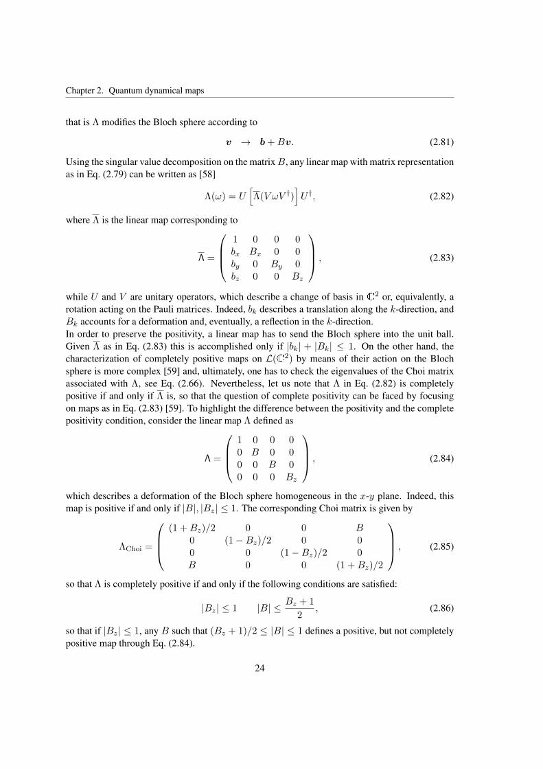
2.2.4 An example: completely positive maps on the Bloch sphere

In order to give an explicit example of what has been presented so far, let us consider the simplestquantum system, namely the two-level system associated with the Hilbert space C2.An orthonormal basis on the Banach space L(C2) of linear operators on C2 is provided by1/√

2, σk/√

2k=x,y,z

, where

σx =

(0 11 0

)σy =

(0 −ii 0

)σz =

(1 00 −1

)(2.77)

denote the usual Pauli matrices. The set of 2×2 positive definite matrices with unit trace representsthe set S(C2) of physical states. Any such matrix can be written as

ρ(v) =1

2(1+ v · σ) , (2.78)

where σ is the vector with components σx, σy, σz and v is a 3-dimensional real vector, such that|v| ≤ 1: S(C2) can be identified with the unit ball inR3. The surface of this ball, known as Blochsphere, represents the set of pure states of the system.Any linear map Λ ∈ LL(C2) can be represented by 4 × 4 complex matrices, according to therepresentations introduced in Sec. (2.2.1). In particular, it is easy to see that if Λ is trace andhermiticity preserving, then the matrix corresponding to Eqs. (2.48) and (2.49) has to be of theform

Λ =

(1 0b B

), (2.79)

with 0, b ∈ R3 and B a 3× 3 real matrix. Thus, the action of a trace preserving linear map Λ ona statistical operator ρ(v) can be expressed as

Λ(ρ(v)) =1

2[1+ (b+Bv) · σ] , (2.80)

23


that is Λ modifies the Bloch sphere according to

v → b+Bv. (2.81)

Using the singular value decomposition on the matrixB, any linear map with matrix representationas in Eq. (2.79) can be written as [58]

Λ(ω) = U[Λ(V ωV †)

]U †, (2.82)

where Λ is the linear map corresponding to

Λ =

1 0 0 0bx Bx 0 0by 0 By 0bz 0 0 Bz

, (2.83)

while U and V are unitary operators, which describe a change of basis in C2 or, equivalently, arotation acting on the Pauli matrices. Indeed, bk describes a translation along the k-direction, andBk accounts for a deformation and, eventually, a reflection in the k-direction.In order to preserve the positivity, a linear map has to send the Bloch sphere into the unit ball.Given Λ as in Eq. (2.83) this is accomplished only if |bk| + |Bk| ≤ 1. On the other hand, thecharacterization of completely positive maps on L(C2) by means of their action on the Blochsphere is more complex [59] and, ultimately, one has to check the eigenvalues of the Choi matrixassociated with Λ, see Eq. (2.66). Nevertheless, let us note that Λ in Eq. (2.82) is completelypositive if and only if Λ is, so that the question of complete positivity can be faced by focusingon maps as in Eq. (2.83) [59]. To highlight the difference between the positivity and the completepositivity condition, consider the linear map Λ defined as

Λ =

1 0 0 00 B 0 00 0 B 00 0 0 Bz

, (2.84)

which describes a deformation of the Bloch sphere homogeneous in the x-y plane. Indeed, thismap is positive if and only if |B|, |Bz| ≤ 1. The corresponding Choi matrix is given by

ΛChoi =

(1 +Bz)/2 0 0 B

0 (1−Bz)/2 0 00 0 (1−Bz)/2 0B 0 0 (1 +Bz)/2

, (2.85)

so that Λ is completely positive if and only if the following conditions are satisfied:

|Bz| ≤ 1 |B| ≤ Bz + 1

2, (2.86)

so that if |Bz| ≤ 1, any B such that (Bz + 1)/2 ≤ |B| ≤ 1 defines a positive, but not completelypositive map through Eq. (2.84).

24


2.2.5 Completely positive maps and reduced dynamics of open quantum systems

To conclude this chapter, we show how the formalism of linear maps on operator spaces introducedin the previous paragraphs applies to the description of the dynamics of open quantum systems.An open quantum system is a quantum system interacting with another system, the environment.As said in section (2.1.3), the system and the environment are the two subsystems of a compositetotal system. It is usually assumed that the latter is closed, thus evolving through a unitary dy-namics. However, the complete description of the entire dynamics is often too complicated to beperformed explicitly, even by means of numerical techniques. Moreover, from the experimentalpoint of view, one can generally control only on a small part of the full system. In any case, evenif one could characterize the whole set of degrees of freedom, he would get an intractable amountof information, most of which useless for a reasonable description of the system. One is thereforedriven to look for a simpler description in terms of a restrict set of relevant dynamical variables,performing an average over the remaining degrees of freedom. Indeed, the border between systemand environment is not assigned a-priori, but ultimately depends on the physical quantities actuallymeasurable in the experiment, see also Chapter 6.Let HS be the Hilbert space associated with the open system and HE the Hilbert space associ-ated with the environment. The open system is often referred to as reduced system. We use thesubscript S for operators onHS and the subscript E for operators onHE . Since one is only inter-ested in observables related to the open system, it is convenient to introduce the statistical operatorassociated with the state of the open system, or reduced state, see Eq. (2.31):

ρS = trE[ρSE ], (2.87)

where trE is the partial trace over HE and represents an average over the environmental degreesof freedom. The total system evolves through a unitary dynamics, which is fixed by the totalHamiltonian

H(t) = HS(t)⊗ 1E + 1S ⊗HE(t) +HI(t), (2.88)

where HS(t) is the self-Hamiltonian of the open system, HE(t) is the self-Hamiltonian of theenvironment and HI(t) is the Hamiltonian describing the interaction between the system and theenvironment. The total Hamiltonian uniquely determines the unitary evolution operator

U(t, t0) = T← exp

[−i∫ t

t0

dsH(s)

], (2.89)

where t0 is the initial time and T← denotes the chronological time-ordering operator, which ordersproduct of time-dependent operators such that their time-arguments increase from right to left.The state of the total system at a time t, ρSE(t), is obtained from the total initial state through theunitary evolution

ρSE(t) = U(t, t0)ρSE(t0)U †(t, t0). (2.90)

This represents a very special case of the completely positive trace preserving transformation mapspresented in the previous paragraphs, see Eq. (2.60) and Eq. (2.68).

25


By taking the partial trace over the degrees of freedom of the environment in Eq. (2.90), the totalinitial state ρSE(t0) is mapped to the state of the open system at a time t,

ρS(t) = trE [U(t, t0)ρSE(t0)U †(t, t0)]. (2.91)

In this way, one establishes a family of evolution maps from the set of states of the total system tothe set of states of the open system, according to

ρSE(t0) 7→ ρS(t) = Υ(t, t0)ρSE(t0) = trE [U(t, t0)ρSE(t0)U †(t, t0)] (2.92)

Note that these are linear, trace preserving and completely positive maps8, since the partial traceis completely positive [3] and the composition of two completely positive maps is completelypositive. However, it is clear that in order to give a self-consistent description of the dynamicsof the open quantum system one has to introduce a map on the set of states of the open system,associating to any reduced initial state ρS(t0) the corresponding state at a time t, ρS(t). If theopen system and the environment are initially in a product state

ρSE(t0) = ρS(t0)⊗ ρE(t0) (2.93)

with a fixed environmental state ρE(t0), Eq. (2.91) allows to define a linear map Λ(t, t0) from thestate space of the open system into itself,

ρS(t0) 7→ ρS(t) = Λ(t, t0)ρS(t0) = trE

[U(t, t0) ρS(t0)⊗ ρE(t0)U †(t, t0)

]. (2.94)

By means of the spectral decomposition of the fixed environmental state ρE(t0), one can showthat the linear map Λ(t, t0) is completely positive:

ρS(t) = TrE [U(t, t0)ρS(t0)⊗ ρE(t0)U †(t, t0)]

=∑k

〈uk|U(t, t0)ρS(t0)⊗

(∑k′

pk′ |vk′〉〈vk′ |

)U †(t, t0)|uk〉

=∑kk′

〈uk|√pk′U(t, t0)|vk′〉ρS(t0)〈vk′ |

√pk′U

†(t, t0)|uk〉

=∑kk′

Mkk′(t, t0)ρS(t0)M †kk′(t, t0). (2.95)

Indeed, Λ(t, t0) can be expanded via linearity to the whole set of trace class operators [50], so thatEq. (2.95) represents its Kraus decomposition, see Eq. (2.60), with Kraus operators given by

Mkk′(t, t0) :=√pk′〈uk|U(t, t0)|vk′〉. (2.96)

The trace preserving condition in Eq. (2.68) is satisfied as a consequence of the unitarity ofU(t, t0). Thus, if the total initial state is a product state, the evolution of the open system can

8Indeed, from Eqs. (2.58) and (2.59) one can easily generalize the definition of complete positivity to linear mapsdefined from T (HSE) to T (HS)

26


always be characterized by a one-parameter family of completely positive trace preserving linear(CPT) maps Λ(t, t0)t≥t0 .9 The latter are usually called reduced dynamical maps. As will bediscussed in more details in Chapter 5, in the presence of initial correlations between the systemand the environment, the very existence of reduced dynamical maps becomes problematic. On theother hand, every CPT map can be seen as a reduced dynamical map with a product total initialstate. Consider the finite dimensional Hilbert space H = CN : assigned a completely positivetrace preserving linear map Λ on L(CN ), there exist an Hilbert space K, a pure state |ψ0〉 in Kand a unitary map U : H⊗K → H⊗K such that

Λ(ω) = trK[U (ω ⊗ |ψ0〉〈ψ0|) U †]. (2.97)

The Hilbert space K can be chosen such that its dimension is smaller or equal to the square di-mension of H. This is a corollary of the Stinespring’s dilation theorem [60], which applies moregenerally to completely positive maps between C∗-algebras.The reduced dynamics that can be exactly derived through Eq. (2.94), although very useful asreference models, are actually quite exceptional. One generally deals with a reduced dynamicsthat is obtained after physically motivated approximations. Then, complete positivity is no longerguaranteed, but it has to be checked explicitly. Thus, it is worth stressing that, given a familyof CPT dynamical maps, the construction in Eq. (2.97) concerns the single dynamical maps, ingeneral without providing unique environment and one-parameter group of unitary operators onthe total Hilbert space, from which the whole family of maps can be obtained in an exact way.

9This family of dynamical maps is only defined for t ≥ t0 since the dynamics of an open system is irreversible.More precisely, a linear, trace preserving and completely positive map can be inverted by another linear, trace preservingand completely positive map if and only it is unitary [46].

27

Chapter 3

Master equations

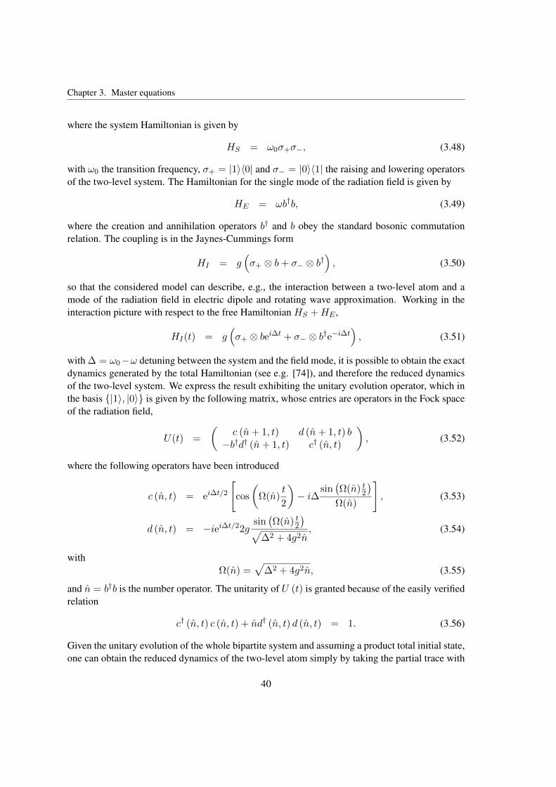
In the previous chapter, we have seen that the evolution of open quantum systems can be charac-terized through a one-parameter family of completely positive trace preserving linear (CPT) maps.However, in concrete physical settings one is often faced with equations of motion rather than withevolution maps and the latter are usually obtained by solving the former.Thus, we now focus on the description of the dynamics of open quantum systems via properequations of motion for the reduced statistical operator, that is, quantum master equations [1]. Itis worth stressing by now that, on the one hand, it is not fully clear which is the most generaloperator structure of the master equations which do provide a well-defined time evolution and,in particular, preserve complete positivity. On the other hand, one would like to link, in a pos-sibly intuitive way, operator structures giving a sensible dynamical evolution with microscopicinformation on the physics of the system of interest. An important case in which both these ap-proaches, phenomenological and microscopic, are well understood and successfully applied isgiven by semigroup dynamics [14, 15].In the first section, we focus on to what extent every open-system dynamics can be described byboth local and non-local in time master equations. We first show that time-local and integrodiffer-ential equations of motion can be derived from the unitary time evolution of the total system bymeans of projection operator techniques. Time-local master equations are not necessarily well de-fined at every time, but they can present isolated singularities. Then, we describe the connectionsbetween a generic family of dynamical maps and the corresponding local and non-local masterequations, also by means of the representations introduced in Sec. (2.2). Finally, we provide thegeneral structure of time-local as well as integrodifferential master equations which guaranteetrace and hermiticity preservation.In the second section, we apply the analysis presented in the first section to a concrete physicalmodel [28]. Namely, we obtain the exact time-local and integrodifferential equations of motion ofa two-level system coupled to a bosonic reservoir consisting first of a single mode of the quantizedelectromagnetic field initially in a thermal state, and then in a collection of quantum harmonic os-cillators initially in the vacuum state. Furthermore, we consider the more general and not exactlysolvable case in which the collection of harmonic oscillators is initially in a thermal state. Weapply a perturbation expansion to the time-local master equation derived via projection operator

29

Chapter 3. Master equations

techniques and we show, in particular, that the operator structures of local and non-local masterequations can strongly differ, also depending on the state of the bath.In the last section, we deal with the problem of identifying those master equations which preservethe complete positivity of the evolution. We first focus on quantum dynamical semigroups. Thefull characterization of the structure of their generators provides a necessary and sufficient con-dition for master equations to be well-defined on an entire class of dynamics, that are significantboth from a mathematical and a physical point of view. The latter aspect is connected with theconcept of Markovianity in the dynamics of open quantum systems, which will be the main sub-ject of the next chapter. We further present two natural generalizations of quantum semigroups,one that is typically obtained from time-local master equations, the other from integrodifferentialmaster equations. Furthermore, we show by means of a simple example some of the problemsthat arise when trying to characterize in full generality those master equations which guarantee acompletely positive evolution.

3.1 Local versus non-local description of reduced dynamics

3.1.1 Integrodifferential and time-local equations of motion from projection oper-ator techniques

Now, we want to derive a closed equation of motion for the dynamics of an open system, startingfrom the unitary time evolution of the corresponding total system and exploiting projection opera-tor techniques [1]. By differentiating the evolution map in Eq. (2.90) with respect to time, one getsthe Liouville-von Neumann master equation for the statistical operator of the total system, that ininteraction picture reads

d

dtρSE(t) = −i [HI(t), ρSE(t) ] ≡ L(t)ρSE(t), (3.1)

where, assuming for simplicity a time independent Hamiltonian H and defining H0 = HS ⊗ 1+1⊗HE , the Hamiltonian in interaction picture is HI(t) = exp(iH0t)HI exp(−iH0t). The basicidea behind the projection operator techniques is to regard the trace over the degrees of freedomof the environment as a formal projection

ρSE 7→ PρSE = trE [ ρSE ]⊗ ρE ≡ ρS ⊗ ρE , (3.2)

with ρE fixed environmental state. The state PρSE is called relevant part of the total state, sinceit allows to reconstruct the open system dynamics, as one can see from the relation

ρS = trE [PρSE ]. (3.3)

On the same way, one can introduce a further map Q defined as

QρSE = ρSE − PρSE . (3.4)

30

3.1. Local versus non-local description of reduced dynamics

Note that P and Q are a pair of complementary projectors on the state space S(H) of the totalHilbert spaceH = HS⊗HE , since they satisfy P+Q = 1, P 2 = P,Q2 = Q and PQ = QP = 0.From Eq. (3.3), it is clear that, by deriving a closed equation of motion for the relevant partPρSE(t), one equivalently gets a closed equation of motion for the reduced state ρS(t). Applyingthe two projectors P and Q to Eq. (3.1), one has

d

dtPρSE(t) = P

d

dtρSE(t) = PL(t)ρSE(t) = PL(t)PρSE(t) + PL(t)QρSE(t),

d

dtQρSE(t) = Q

d

dtρSE(t) = QL(t)ρSE(t) = QL(t)PρSE(t) +QL(t)QρSE(t), (3.5)

where we used P +Q = 1 to derive the last equalities. The formal solution of the second equationfor a total initial state ρSE(t0) is given by

QρSE(t) = D(t, t0)QρSE(t0) +

∫ t

t0

dsD(t, s)QL(s)PρSE(s), (3.6)

where we introduced

D(t, s) ≡ T← exp

[∫ t

sds′QL(s′)

]. (3.7)

Inserting Eq. (3.6) into the equation of motion for the relevant part of the total state, the followingequation, known as Nakajima-Zwanzig equation [61, 62], is obtained:

d

dtPρSE(t) = PL(t)D(t, t0)QρSE(t0)+PL(t)PρSE(t)+

∫ t

t0

dsPL(t)D(t, s)QL(s)PρSE(s).

(3.8)We emphasize that Eq. (3.8) has been derived in an exact way from the total unitary evolutionand it holds for any total initial state. However, in the following we will consider product initialstates ρSE(t0) = ρS(t0) ⊗ ρE , so that the first term at the right hand side of Eq. (3.8) vanishes.Furthermore, one usually has that PL(t)P = 01 and then the Nakajima-Zwanzig equation reducesto

d

dtPρSE(t) =

∫ t

t0

dsKNZ(t, s)PρSE(s), (3.9)

withKNZ(t, s) = PL(t)D(t, s)QL(s)P. (3.10)

The right hand side of Eq. (3.9) consists in an integral over the past history of the system in thetime interval [t0, t] and then it describes the memory effects on the reduced dynamics due to theinteraction with the environment. The concept of memory effect plays a basic role in the definitionof Markovianity, as will be widely discussed. The term KNZ(t, s) is thus called memory kernel.In the following we will focus on time homogeneous kernel, i.e. such that K(t, s) = K(t − s),which is the case for a stationary state ρE .

1In any case, given a stationary ρE , one can always define a new interaction Hamiltonian with a shifted origin ofthe energy such that this relation holds [63].

31


The same techniques lead to time-local equations of motion for the relevant part of the dynamics.This is achieved by introducing a backward propagator (T→ indicates the anti-chronological time-ordering)

G(t, s) = T→ exp

[−∫ t

sds′L(s′)

], (3.11)

such that ρSE(s) = G(t, s)ρSE(t). Inserting ρSE(s) = G(t, s)(P + Q)ρSE(t) in Eq. (3.6) anddefining

Σ(t) =

∫ t

t0

dsD(t, s)QL(s)PG(t, s), (3.12)

one gets

QρSE(t) = [1− Σ(t)]−1Σ(t)PρSE(t) + [1− Σ(t)]−1D(t, t0)QρSE(t0), (3.13)

so that the first of Eq. (3.5) gives the time-convolutionless equation of motion [64, 65, 66, 67]

d

dtPρSE(t) = KTCL(t)PρSE(t) + I(t)QρSE(t0), (3.14)

where we introduced the time-local generator

KTCL(t) = P L(t)[1− Σ(t)]−1P (3.15)

and the inhomogeneous term

I(t) = PL(t)[1− Σ(t)]−1D(t, t0)Q, (3.16)

which vanishes for a product initial state. The existence of the inverse map [1 − Σ(t)]−1 is notalways guaranteed, so that Eq. (3.14) is not necessarily well-defined for any t ≥ t0. Contrary tothe integrodifferential equation in Eq. (3.8), the time-convolutionless equation cannot be generallyobtained from the full unitary dynamics by projection operator techniques for every time t ≥ t0.Nevertheless, we will see in Sec. (3.2.4) how the inverse map does always exist for small valuesof t− t0 and for small values of the coupling constant.

3.1.2 From linear maps to master equations

By means of projection operator techniques one can thus always derive master equations for thereduced statistical operator which are in integrodifferential form, the Nakajima-Zwanzig masterequations2

d

dtρS(t) =

∫ t

t0

dτKNZ(t− τ)ρS(τ), (3.17)

2For the sake of clarity, we emphasize that in the following we will refer to this and the next equation to indicategeneric integrodifferential and time-local master equations, respectively, not necessarily obtained by projection operatortechniques, neither necessarily equivalent to the full unitary evolution. We have employed the notation KTCL for atime-local generator acting on the total system and obtained by projection operator techniques, while we use KTCL fora generic time-local generator acting on the reduced system and KTCL for the matrix associated with its representationgiven by Eqs. (2.41) and (2.42), see Sec. (2.2.1). Fully analogous notations are used for the memory kernel.

32


or in time-local form, the time-convolutionless master equations

d

dtρS(t) = KTCL(t)ρS(t). (3.18)

Indeed, this can be accomplished simply by taking the partial trace in, respectively, Eq. (3.9) andEq. (3.14) and using PρSE(t) = ρS(t)⊗ ρE . For simplicity, from now on we will set t0 = 0 and,except if otherwise stated, we will omit the subscript S, so that the reduced statistical operatorat a time t will be indicated as ρ(t). Both Eq. (3.9) and (3.14) are exact and then they are asdifficult to solve as the initial Liouville-von Neumann master equation. Therefore, perturbationexpansions are usually employed in order to get a description of the reduced dynamics which canbe explicitly accessed, analytically as well as numerically. An example for the time-local masterequation of a two-level system will be given in Sec. (3.2.4). Moreover, the dynamics of openquantum systems is often studied through equations of motion, being local as well as non-localin time, that are not obtained from the full unitary evolution, but that are introduced on the basisof phenomenological ansatz in order to properly describe some observed phenomenon. In thisparagraph, we emphasize that also in these situations the local and the non-local description ofreduced dynamics are actually equivalent, in the sense that the same dynamics can be describedby both a time-convolutionless and an integrodifferential master equation. In fact, we connect ageneric one-parameter family of linear maps describing an open system evolution to a local aswell as to a non-local master equation: indeed, different forms of equations might admit the verysame solutions.Consider a one-parameter family of reduced dynamical maps Λ(t, 0)t≥0, where every Λ(t, 0) isa completely positive trace preserving linear map defined on the whole set L(CN ) of linear op-erators on CN . Indeed, the physical meaning of these maps as representatives of transformationsof quantum systems is well established on the set S(CN ) of physical states. However, since thereare sets of statistical operators spanning L(CN ), a linear map on S(CN ) uniquely defines a linearmap on L(CN ). Under the hypotheses that Λ(t, 0) can be derived with respect to time3 and thatthe inverse linear map Λ−1(t, 0) exists, it is straightforward to see that a time-local equation as inEq. (3.18) is satisfied upon identifying

KTCL(t) =dΛ(t, 0)

dtΛ−1(t, 0). (3.19)

It is worth stressing that, contrary to the reduced dynamical map Λ(t, 0), the inverse map Λ−1(t, 0)is not completely positive, unless Λ(t, 0) is unitary. In any case, the existence of a linear mapΛ−1(t, 0) such that Λ(t, 0)Λ−1(t, 0) = 1 is indeed not a priori guaranteed. As a consequence, itmay well happen that at some times t ∈ R+ a time-local generator cannot be defined or, even,there is an infinity of generators corresponding to the same evolution [56]. However, apart fromthese critical points, the reduced dynamics can be safely characterized with a time-local masterequation.

3Given a normed spaceX and a function f : R→ X , one says that f can be derived in t ∈ R if there is an elementx ∈ X such that the following implication holds: hn , hn ∈ R, hn 6= 0 ∀n, |hn| → 0⇒ ‖ f(t+hn)−f(t)

hn− x‖ → 0,

and x is the derivative of f in t.

33


On a similar footing, by exploiting the Laplace transform, we can derive a master equation inintegrodifferential form as in Eq. (3.17). We recall that the Laplace transform v(u) of the functionor map v(t) is defined as

v(u) =

∫ ∞0

dt v(t) e−ut. (3.20)

Since dv/dt = uv(u)− v(0) and the Laplace transform of the convolution between v(t) and w(t)is given by the product v(u) w(u), from Eq. (3.17) one has

uρ(u)− ρ(0) = KNZ(u) ρ(u). (3.21)

Then, since ρ(u) = Λ(u)ρ(0), we come to

KNZ(u) = u1− Λ−1(u). (3.22)

This relation is sometimes equivalently written as [68], see also Sec. (6.1.4),

KNZ(u) =uG(u)

1 + G(u), (3.23)

where Λ(t, 0) = 1+∫ t

0 dsG(s), so that uΛ(u)− 1 = G(u).Furthermore, it is useful to express the previous relations by means of matrix representations. Therepresentation given by Eqs. (2.41) and (2.42) is the most convenient for this purpose since itassociates compositions of linear maps with compositions of matrices, so that Eq. (3.19) reads

KTCL(t) =dΛ(t, 0)

dtΛ−1(t, 0), (3.24)

while Eq. (3.22) can be written in matrix form as

KNZ(u) = u1− Λ−1(u). (3.25)

The dynamical map Λ(t, 0) has been our starting point since in this way we could directly showthrough Eqs. (3.19) and (3.22) that the very same dynamics can be described by both a local anda non-local master equation. However, as recalled in the introduction to this chapter, one usuallydeals with master equations, so that dynamical maps are obtained by solving them. Given a time-local master equation as in Eq. (3.18), the formal solution is obtained through the Dyson series

Λ(t, 0) = T← exp

[∫ t

0dτKTCL(τ)

]≡ 1+

∞∑k=1

1

k!

∫ t

0. . .

∫ t

0T←KTCL(t1) . . .KTCL(tk)dt1 . . . dtk, (3.26)

where T← denotes the chronological time-ordering operator and the convergence of the series isguaranteed since we are dealing with finite dimensional systems and then the time-local generator

34


KTCL(t) is bounded. On the other hand, for an integrodifferential equation one has to take theinverse Laplace transform of, see Eq. (3.22),

Λ(u) =(u1− KNZ(u)

)−1. (3.27)

Finally, let us note that the equivalence between the local and the non-local description of open-system dynamics can be shown also by means of the damping bases [69]. In fact, consider adynamical map Λ(t, 0) which is the solution of a Nakajima-Zwanzig master equation, i.e. it satis-fies Eq. (3.27), and let it be written as, see Eq. (2.70),

Λ(t, 0)ω =∑α

λα(t)Tr [ς†α(t)ω]$α(t) ω ∈ L(CN ), (3.28)

where the operators $α(t)α=1,...,N2 and ςα(t)α=1,...,N2 define pairs of damping bases, seeEq. (2.72), which are generally different at different times. The inverse map can be formallydefined (for t such that λα(t) 6= 0 ∀α ) as

Λ−1(t, 0)ω =∑α

λ−1α (t)Tr [ς†α(t)ω]$α(t) ω ∈ L(CN ), (3.29)

and, through Eq. (3.19), one can obtain the time-local generator

KTCL(t)ω =∑αβ

Kαβ(t)Tr [ς†β(t)ω] ω ∈ L(CN ), (3.30)

where the terms Kαβ(t) include the operators $α(t) and their time derivatives, see [69]. If thedamping bases do not depend on time, Eq. (3.30) reduces to

KTCL(t)ω =∑α

λα(t)

λα(t)Tr [ς†α ω]$α ω ∈ L(CN ), (3.31)

in full analogy with the matrix representation given by Eqs. (2.41), (2.42) and (3.24), with thedifference that the time-local generator KTCL(t) is now expanded on its, non orthogonal, eigen-basis. Note that if the damping bases do not depend on time, dynamical maps as well as time-localgenerators at different times commute

[Λ(t, 0),Λ(s, 0)] = 0,

[KTCL(t),KTCL(s)] = 0, (3.32)

and then in Eq. (3.26) the chronological time-ordering operator can be omitted. In Sec. (3.3.3)we will briefly come back to this specific case, which has been widely analyzed in [48, 70].

35


3.1.3 Trace and hermiticity preservation

As stressed in the previous paragraph, one generally deals with approximated master equationswhich are not equivalent to the exact total unitary evolution, so that a priori they do not guaranteea well-defined time evolution. Consequently, it is of relevance to identify the operator structureof those master equations which do yield a well-defined time evolution. This task has not beenaccomplished with full generality yet. Indeed, the difficulty relies on the request that the cor-responding dynamical maps have to be completely positive4. In this paragraph we show that,however, some general constraints on the structure of the proper master equations can be derivedby asking for trace and hermiticity preservation.Consider a time t ≥ 0 where the inverse of the dynamical map Λ(t, 0) exists, so that a time-localgenerator KTCL(t) is uniquely defined. Then, it has to satisfy5

Tr[KTCL(t)ω] = 0 ∀ω ∈ L(CN )

(KTCL(t)ω)† = KTCL(t)ω† ∀ω ∈ L(CN ), (3.33)

where, indeed, these two conditions express, respectively, trace and hermiticity preservation. Now,consider a linear map Λ on L(CN ) and its representation through Eq. (2.50), where the ma-trix of coefficients Λ′ has entries Λ′αβ , with α, β = 0, . . . N2 − 1, as in Eq. (2.51) for a basisσαα=0,...,N2−1 such that

σ0 = 1/√N

Tr[σα] = 0 α = 1, . . . , N2 − 1. (3.34)

The Lemma 2.3 in [14] shows that if Λ fulfills Tr[Λ(ω)] = 0 for any ω ∈ L(CN ), then it can bewritten as

Λ(ω) = −i [H,ω] +N2−1∑αβ=1

Λ′αβ

(σαωσ

†β −

1

2

σ†βσα, ω

), (3.35)

with the coefficients Λ′αβ given by Eq. (2.51) and

H =1

2i(σ† − σ)

σ =1√N

N2−1∑α=1

Λ′α0σα. (3.36)

Note that the matrix of coefficients in the second term at the right hand side of Eq. (3.35) isobtained from the matrix Λ′ by simply removing the first row and the first column. If we further

4Positivity would be in general even more difficult to be verified than complete positivity, since it is connected tothe action of the map on the whole set of states, rather than to the eigenvalues of the corresponding Choi matrix, seesection (2.2).

5The time-local master equation (3.18) per se implies that the two conditions in Eq. (3.33) are satisfied if KTCL(t)is applied to operators into the image of Λ(t, 0). But if the latter is invertible, than its image has the same dimensionalityof L(CN ) and then the two conditions can be extended to the whole space of linear operators. For our purposes, onecould equivalently start by assuming the validity of Eq. (3.33).

36


ask that the linear map Λ is hermiticity-preserving, then the matrix Λ′ is hermitian, see Sec. (2.2.1):explicitly,

Λ′αβ = Λ′∗βα ∀α, β = 0, . . . N2 − 1. (3.37)

Then, the matrix of coefficients in Eq. (3.35) is hermitian, as well.Coming back to the time-local generator KTCL(t), we observe that Eqs. (3.35)-(3.37) can beapplied for any fixed time t, with respect to the same basis, because of Eq. (3.33). Thus, weconclude that every time-local master equation satisfying Eq. (3.33) can be written as

d

dtρ(t) = −i [H(t), ρ(t)] +

N2−1∑αβ=1

KαβTCL(t)

(σαρ(t)σ†β −

1

2

σ†βσα, ρ(t)

), (3.38)

with

H(t) =1

2i(σ(t)† − σ(t))

σ(t) =1√N

N2−1∑α=1

Kα0TCL(t)σα, (3.39)

where the basis σαα=0,...,N2−1 fulfills Eq. (3.34) and the coefficients Kαβ ∗TCL(t) = Kβα

TCL(t) aregiven by, see Eq. (2.51),

KαβTCL(t) =

N2−1∑γ=0

Tr[σβ σ†γ σ†αKTCL(t)σγ ] α, β = 0, . . . N2 − 1. (3.40)

The first term of the time-local generator in Eq. (3.38) represents a unitary contribution to thedynamics, generated by the self-adjoint operator H(t), while the second term describes the dis-sipation and the decoherence on the open system due to the interaction with the environment[1], see also Chapter 6. The decomposition into a unitary and a dissipative part provided byEqs. (3.38)-(3.40) is unique, in the sense that no further contributions to H(t) can be derived fromthe dissipative part of the generator [71]. Furthermore, the matrix of coefficients in Eq. (3.38) ishermitian since it is obtained from the hermitian matrix with entries as in Eq. (3.40) by removingthe first row and the first column. Then, for any time t there is a unitary matrix V(t) such thatKαβ

TCL(t) =∑

γ Vαγ(t)kγ(t)V ∗βγ(t), for α, β = 1, . . . , N2 − 1, with kα(t) real functions of time.The time-local master equation in Eq. (3.38) can then be written in diagonal form as

d

dtρ(t) = −i [H(t), ρ(t)] +

N2−1∑α=1

kα(t)

(σα(t)ρ(t)σ†α(t)− 1

2

σ†α(t)σα(t), ρ(t)

), (3.41)

where the operators

σα(t) =

N2−1∑β=1

Vβα(t)σβ (3.42)

37


for α = 1, . . . , N2 − 1 plus σ0 = σ0 provide, at any fixed time t, an orthonormal basis in L(CN )with respect to the Hilbert-Schmidt scalar product. Note that the coefficients kα(t) and the opera-tors σα(t) do depend on time since the eigenvalues and eigenvectors of the matrix of coefficientsin Eq. (3.38) are generally different at different times. The diagonal form as in Eqs. (3.41) and(3.42) can be considered the canonical form of the time-local generator, since it is obtained fromthe diagonalization of the coefficient matrix, see the discussion after Eq. (2.64).Let us now consider integrodifferential master equations as in Eq. (3.17), that in Laplace trans-form reads as in Eq. (3.21). If Λ−1(u) exists, then Eq. (3.21) implies that the memory kernel hasto satisfy Tr[KNZ(u)ω] = 0, ∀ω ∈ L(CN ), compare with the first of Eq. (3.33). Thus, we canonce again use the representation of linear maps given by Eqs. (2.50) and (2.51) and apply, for anyfixed u, Eqs. (3.35) and (3.36), thus coming to

KNZ(u)ω = −i [H(u), ω] +N2−1∑αβ=1

KαβNZ(u)

(σαωσ

†β −

1

2

σ†βσα, ω

), (3.43)

with H(u) as in Eq. (3.39) and KαβNZ(u) as in Eq. (3.40), but, of course, with KNZ(u) instead

of KTCL(t). Moreover, Eq. (3.21) implies that for u ∈ R the Laplace transform of the memorykernel is hermiticity preserving as well, i.e., (KNZ(u)ω)† = KNZ(u)ω† for any ω ∈ L(CN ).Then, the matrix of coefficients in Eq. (3.43) is hermitian, i.e. Kαβ

NZ(u) = (KβαNZ)∗(u). Due to the

identity principle, the equality of these two functions can be extended to their common region ofanalyticity. By exploiting the invertibility of the Laplace transform, we get the same equality forthe coefficients of the memory kernel in the temporal domain, i.e., Kαβ

NZ(t) = (KβαNZ)∗(t). Thus,

we can write the memory kernel as

KNZ(t)ω = −i [H(t), ω] +N2−1∑α

rα(t)

(σα(t)ωσ†α(t)− 1

2

σ†α(t)σα(t), ω

), (3.44)

where, indeed the time-dependent real coefficients ra(t) and linear operators σα(t) are obtainedby diagonalizing the matrix with elements Kαβ

NZ(t), compare with Eq. (3.42).Conversely, consider a time local master equation of the form

d

dtρ(t) = −i [H(t), ρ(t)] +

N2−1∑α=1

kα(t)


2


)(3.45)

as well as an integrodifferential master equation of the form

d

dtρ(t) = −i

∫ t

0dτ [H(t− τ), ρ(τ)] (3.46)

+N2−1∑α=1

∫ t

0dτ rα(t− τ)

(σα(t− τ)ρ(τ)σ†α(t− τ)− 1

2

σ†α(t− τ)σα(t− τ), ρ(τ)

),

38

3.2. Local versus non-local master equation for the dynamics of a two-level system

with H†(t) = H(t), σα(t) ∈ L(CN ) generic linear operators on CN , kα(t) and rα(t) genericreal functions of t. Then, one can see6 that they guarantee trace and hermiticity preservation.We want to remark that Eq. (3.45) and Eq. (3.46) are not necessarily always the most convenientway in order to express, respectively, time-local generators and memory kernels. In some cases,different structures can be more useful to determine the corresponding dynamical maps or to checkwhether complete positivity is preserved. An example is given by the master equation introducedin [72], see also [73] where its complete positivity for a two-level system is studied.

3.2 Local versus non-local master equation for the dynamics of atwo-level system

In this section, we apply what has been presented in an abstract way in the previous section toa realistic physical model, simple enough to be exactly treated in detail, but already allowing togive some general remarks. Namely, in the first three paragraphs we consider a two-level systemcoupled first to a single mode of the radiation field and later to a bath of harmonic oscillators atzero temperature, via a Jaynes-Cummings type of interaction. By exploiting the knowledge ofthe exact unitary evolution, and therefore of the reduced dynamics, we can derive the exact time-convolutionless and Nakajima-Zwanzig master equations. Their operator structures are shown tobe generally different, also depending on the environmental state.Indeed the exact knowledge of the full time evolution is feasible only for exceptional cases. Thedetailed analysis of such cases, however, proves quite useful in understanding the basic features ofthe description of open system dynamics; in particular, it puts into evidence the strict relationshipbetween the different quantities which appear in evolution equations, showing that phenomenolog-ical ansatze are in general not easily feasible. Moreover, the exact comprehensive study performedin these cases allows to point out general features which can be useful for phenomenological orperturbative treatments, as that presented in the last part of the section. Here, we take into accounta more general situation, where the exact solution is no longer available. In particular, we con-sider an environment consisting of a bath of harmonic oscillators in a thermal state, expanding thetime-local generator derived by means of projection operator techniques up to second order. Thefourth order term of the expansion is given in Appendix F.The material of this section is for the most part contained in [28].

3.2.1 Jaynes-Cummings model and exact reduced dynamics

We consider a two-level system coupled to a single mode of the radiation field according to thetotal Hamiltonian

H = HS +HE +HI , (3.47)6In fact, the time-local generator in Eq. (3.45) satisfies Eq. (3.33), while the memory kernel in Eq. (3.46) satisfies

the analogous relations in Laplace transform. Then, by means of, respectively, Eq. (3.26) and Eq. (3.27), one has thatthe corresponding evolution maps are trace and hermiticity preserving.

39


where the system Hamiltonian is given by

HS = ω0σ+σ−, (3.48)

with ω0 the transition frequency, σ+ = |1〉〈0| and σ− = |0〉〈1| the raising and lowering operatorsof the two-level system. The Hamiltonian for the single mode of the radiation field is given by

HE = ωb†b, (3.49)

where the creation and annihilation operators b† and b obey the standard bosonic commutationrelation. The coupling is in the Jaynes-Cummings form

HI = g(σ+ ⊗ b+ σ− ⊗ b†

), (3.50)

so that the considered model can describe, e.g., the interaction between a two-level atom and amode of the radiation field in electric dipole and rotating wave approximation. Working in theinteraction picture with respect to the free Hamiltonian HS +HE ,

HI(t) = g(σ+ ⊗ bei∆t + σ− ⊗ b†e−i∆t

), (3.51)

with ∆ = ω0−ω detuning between the system and the field mode, it is possible to obtain the exactdynamics generated by the total Hamiltonian (see e.g. [74]), and therefore the reduced dynamicsof the two-level system. We express the result exhibiting the unitary evolution operator, which inthe basis |1〉, |0〉 is given by the following matrix, whose entries are operators in the Fock spaceof the radiation field,

U(t) =

(c (n+ 1, t) d (n+ 1, t) b

−b†d† (n+ 1, t) c† (n, t)

), (3.52)

where the following operators have been introduced

c (n, t) = ei∆t/2

[cos

(Ω(n)

t

2

)− i∆

sin(Ω(n) t2

)Ω(n)

], (3.53)

d (n, t) = −iei∆t/22gsin(Ω(n) t2

)√∆2 + 4g2n

, (3.54)

withΩ(n) =

√∆2 + 4g2n, (3.55)

and n = b†b is the number operator. The unitarity of U (t) is granted because of the easily verifiedrelation

c† (n, t) c (n, t) + nd† (n, t) d (n, t) = 1. (3.56)

Given the unitary evolution of the whole bipartite system and assuming a product total initial state,one can obtain the reduced dynamics of the two-level atom simply by taking the partial trace with

40


respect to the environmental degrees of freedom, see Eq. (2.94). Taking U(t) as in Eq. (3.52)and considering an environmental state commuting with the number operator, [ρE , n] = 0, so thatin particular both the vacuum and a thermal state can be dealt with, one comes to the followingexplicit expression for the action of the map Λ(t, 0):

ρ(0) =

(ρ11 ρ10

ρ01 ρ00

)7→ ρ(t) = Λ(t, 0)ρ(0) (3.57)

=

(ρ00 (1− α(t)) + ρ11β (t) ρ10γ (t)

ρ01γ∗(t) ρ00α (t) + ρ11 (1− β(t))

).

The effect of the interaction with the bath is contained in the time dependent coefficients α(t), β(t)and γ(t), which are given by the following expectation values over the state of the environmentρE , see Eq. (2.20):

α(t) = 〈c† (n, t) c (n, t)〉E ,β(t) = 〈c† (n+ 1, t) c (n+ 1, t)〉E ,γ(t) = 〈c (n, t) c (n+ 1, t)〉E . (3.58)

Now that we have obtained the completely positive map Λ(t, 0) giving the exact reduced timeevolution of the considered two-level system, we can exploit the representations of linear mapsintroduced in the previous chapter. Consider in particular the representation given by Eqs. (2.41)and (2.42) with respect to the orthonormal basis of operators

1√21, 1√

2σk

, where now σk denote

the usual Pauli operators, see Eq. (2.77). This choice leads to the following expression for thematrix Λ(t) associated with the time evolution map Λ(t, 0):

Λ(t, 0) =

1 0 0 00 γR(t) γI(t) 00 −γI(t) γR(t) 0

β(t)− α(t) 0 0 β (t) + α(t)− 1

, (3.59)

where the coefficients defined in Eq. (3.58) appear, and we denote with R and I real and imagi-nary part of a given function: γ = γR + iγI . For any fixed time t, the linear map in Eq. (3.59)describes a translation along the z-axis plus a rotation and a contraction of the Bloch sphere, seeSec. (2.2.4); recall that the complete positivity is guaranteed since we are dealing with the exactreduced dynamics.

3.2.2 Exact time-convolutionless and Nakajima-Zwanzig master equations

With the aid of the exact time evolution, and using the representation of maps in terms of matrices,we will now explicitly obtain a local and a non-local exact equation of motion for the reduced-

41


system dynamics. Starting from Eq. (3.59) and Eq. (3.24) one obtains for the model of interest

KTCL(t) =

0 0 0 0

0 Re[γ(t)γ(t)

]Im[γ(t)γ(t)

]0

0 − Im[γ(t)γ(t)

]Re[γ(t)γ(t)

]0

[1−2β(t)]α(t)−[1−2α(t)]β(t)β(t)+α(t)−1 0 0 β(t)+α(t)

β(t)+α(t)−1

, (3.60)

and the expression is well defined provided the determinant

det Λ(t) = |γ(t)|2 [α(t) + β(t)− 1] (3.61)

is different from zero. On a similar footing one can consider the Laplace transform of Eq. (3.59),given by the matrix Λ(u) with determinant

det Λ(u) =[γR

2 (u) + γI2(u)

] [ α(u) + β(u)

u− 1

u2

], (3.62)

and using Eq. (3.25) one further obtains

KNZ(u) =

0 0 0 0

0 u− γR(u)

γR2(u)+γI

2(u)

γI(u)

γR2(u)+γI

2(u)0

0 − γI(u)

γR2(u)+γI

2(u)u− γR(u)

γR2(u)+γI

2(u)0

u2[α(u)−β(u)]1−u[α(u)+β(u)]

0 02u−u2[α(u)+β(u)]1−u[α(u)+β(u)]

,(3.63)

which upon inverse Laplace transform provides the exact Nakajima-Zwanzig integral kernel. Asit appears, working with the matrix representation has proved very convenient to easily obtainthe maps fixing the time-local and integrodifferential equations of motion for the model, given byEq. (3.18) and Eq. (3.17) respectively, in terms of the dynamical map Eq. (3.57).

Maps in canonical form

We now recast the obtained maps in operator form, to better compare with previous work andappreciate the difference in the obtained expressions. In particular, we follow the procedure pre-sented in the previous section that allows to get the canonical form of linear maps.Consider a matrix of the form

A =

0 0 0 00 Er Ei 00 −Ei Er 0X 0 0 Y

(3.64)

with respect to the representation given by Eqs. (2.41) and (2.42), in the basis

1√21, 1√

2σk

,

where recall that now σk denote the usual Pauli operators. To move into the representation given

42


by Eqs. (2.50) and (2.51), one can directly connect the coefficients of the matrix Λ in Eq. (2.42)and those of the matrix Λ′ in Eq. (2.51). In fact, by sobstituting Eq. (2.41) into Eq. (2.51), one has

Λ′α′β′ =∑αβ

Λαβ Tr[σβ′σ†βσ†α′σα]. (3.65)

Indeed, last term in the previous relation defines a 16× 16 matrix, which expresses the change ofbasis in LL(CN ) from Eαβαβ=1,...,4 to Fαβαβ=1,...,4, see Eqs. (2.44) and (2.45). In fact, itholds, see Eq. (2.43),

〈〈Fα′β′ , Eαβ〉〉 = Tr[σβ′σ†βσ†α′σα]. (3.66)

Applying Eq. (3.65) to the matrix A in Eq. (3.64), we come to

A′ =

Er + Y/2 0 0 −iEi +X/2

0 −Y/2 −iX/2 00 iX/2 −Y/2 0

iEi +X/2 0 0 Y/2− Er

. (3.67)

The basis we are using satisfies Eq. (3.34). Then, to obtain the canonical form of the linear map Aassociated with A and A′, we simply have to diagonalize the matrix which is obtained by removingthe first row and the first column to Eq. (3.67), see Eqs. (3.41) and (3.42), and to introduce anHamiltonian term through Eq. (3.39). Thus, we get

A(ω) = iEi [σ+σ−, ω] +1

2(X − Y )

[σ+ωσ− −

1

2σ−σ+, ω

](3.68)

−1

2(X + Y )

[σ−ωσ+ −

1

2σ+σ−, ω

]+

1

4(Y − 2Er) [σzωσz − ω] ,

whose last term can be written in alternative ways according to the identities

σzωσz − ω = 4

[σ+σ−ωσ+σ− −

1

2σ+σ−, ω

]= 4

[σ−σ+ωσ−σ+ −

1

2σ−σ+, ω

]. (3.69)

Exploiting this result, one obtains the exact time-convolutionless master equation describing thereduced dynamics of a two-level atom coupled according to the Jaynes-Cummings model to asingle mode of the radiation field, which is of the form Eq. (3.18) with KTCL (t) given by

KTCL(t)ω = i Im

[γ(t)

γ(t)

][σ+σ−, ω] +

[α(t)− 1] β (t)− β(t)α(t)

β(t) + α(t)− 1

[σ+ωσ− −

1

2σ−σ+, ω

]+

[β(t)− 1] α (t)− α(t)β(t)

β(t) + α(t)− 1

[σ−ωσ+ −

1

2σ+σ−, ω

]+

1

4

β(t) + α(t)

β(t) + α (t)− 1− 2 Re

[γ (t)

γ(t)

][σzωσz − ω] . (3.70)

43


In a similar way, one has for the Laplace transform of the memory kernel KNZ(t), appearing inthe exact Nakajima-Zwanzig master equation Eq. (3.17), the expression

KNZ(u)ω = iγI(u)

γR2(u) + γI

2(u)[σ+σ−, ω] +

u [uα(u)− 1]

1− u[α(u) + β(u)

] [σ+ωσ− −1

2σ−σ+, ω

]

+u[uβ(u)− 1

]1− u

[α(u) + β(u)

] [σ−ωσ+ −1

2σ+σ−, ω

]

+1

4

u2[α(u) + β(u)

]1− u

[α(u) + β(u)

] + 2γR(u)

γR2(u) + γI

2(u)

[σzωσz − ω] . (3.71)

Despite being exact these expressions are quite cumbersome, since the functions given in Eq. (3.58),which together with their Laplace transform determine the structure of these operators, depend onthe specific expression of the environmental state. It is therefore convenient to consider a specificchoice, allowing for a more detailed evaluation.

The vacuum case

If the radiation field is in the vacuum state, the functions given in Eq. (3.58) simplify considerably,since α(t)→ 1, while β(t) becomes a function of γ(t) according to β(t)→ |γ(t)|2. The functionγ(t) for the vacuum case is given by the expression

G1(t) = ei∆t/2[cos

(Ω1t

2

)− i ∆

Ω1sin

(Ω1t

2

)], (3.72)

where the superscript recalls that we have a single mode of the radiation field, while Ω1 =√∆2 + 4g2, see Eq. (3.55). These results for the vacuum case greatly simplify the expression

of the obtained master equations, and inserted in Eq. (3.61) show that the time-convolutionlessmaster equation off-resonance is always well defined. The time-local generator for the vacuumcase reads

KVacTCL(t)ω = −ig2∆

1− cos (Ω1t)

Ω1

[cos2

(Ω1t

2

)+

∆2

Ω21

sin2

(Ω1t

2

)]−1

[σ+σ−, ω] (3.73)

+2g2 sin (Ω1t)

Ω1

[cos2

(Ω1t

2

)+

∆2

Ω21

sin2

(Ω1t

2

)]−1 [σ−ωσ+ −

1

2σ+σ−, ω

],

where in particular one directly sees that the coefficient in front of the dissipative term at the r.h.s.of Eq. (3.73) periodically takes on negative values. The choice of the vacuum as bath state brings inimportant simplifications also for the expression of the Nakajima-Zwanzig memory kernel, whichreads

KVacNZ (τ)ω = −ig2 sin (∆τ) [σ+σ−, ω] + 2g2 cos

(√∆2 + 2g2τ

)[σ−ωσ+ −

1

2σ+σ−, ω

]−1

2g2[cos(√

∆2 + 2g2τ)− cos (∆τ)

][σzωσz − ω] , (3.74)

44


which is always well-defined even on-resonance.

3.2.3 Bath of harmonic oscillators at zero temperature

We consider now the case in which the environmental Hamiltonian is a collection of harmonicoscillators

HE =∑k

ωkb†kbk, (3.75)

and the interaction Hamiltonian is replaced by

HI =∑k

(gkσ+ ⊗ bk + g∗kσ− ⊗ b

†k

). (3.76)

This model corresponds, for a Lorentzian spectral density, to the damped Jaynes-Cummings model.The time evolution map for this model, considering the special case of an environment in the vac-uum state, i.e. at zero temperature, has been obtained in [66] and can be expressed as:

ρ(0) =

(ρ11 ρ10

ρ01 ρ00

)7→ ρ(t) = ΛDVac(t)ρ(0) =

(ρ11 |G (t)|2 ρ10G (t)

ρ01G∗ (t) ρ00 + ρ11

(1− |G(t)|2

).

)(3.77)

where ρ(t) = ΛDVac(t)ρ (0), since we are considering the damped model with the bath in thevacuum state. The function G(t) is the solution of the equation

d

dtG(t) = −

∫ t

0dt1f (t− t1)G (t1) G (0) = 1, (3.78)

with f(t) the two-point correlation function given by

f (t− t1) = eiω0(t−t1)〈0|∑k

gkbke−iωkt

∑j

g∗j b†jeiωjt1 |0〉 =

∑k

|gk|2 ei(ω0−ωk)(t−t1), (3.79)

corresponding to the Fourier transform of the spectral density. Starting from Eq. (3.77) one imme-diately obtains for the matrix representation of the time-convolutionless generator the expression

KDVacTCL (t) =

0 0 0 0

0 Re[G(t)G(t)

]Im[G(t)G(t)

]0

0 − Im[G(t)G(t)

]Re[G(t)G(t)

]0

2 Re[G(t)G(t)

]0 0 2 Re

[G(t)G(t)

]

, (3.80)

that in operator form reads

KDVacTCL (t)ω = +i Im

[G(t)

G(t)

][σ+σ−, ω]− 2 Re

[G(t)

G (t)

] [σ−ωσ+ −

1

2σ+σ−, ω

], (3.81)

45


which confirms the result obtained in [1]. One can also determine the expression of the Nakajima-Zwanzig memory kernel, whose Laplace transform is given by

KDVacNZ (u) =

0 0 0 0

0 u− GR(u)

GR2(u)+GI

2(u)

GI(u)

GR2(u)+GI

2(u)

0

0 − GI(u)

GR2(u)+GI

2(u)

u− GR(u)

GR2(u)+GI

2(u)

0

uz(u)−1z(u) 0 0 uz(u)−1

z(u)

, (3.82)

where we have used the notation z(t) = |G(t)|2, leading to

KVacNZ (u)ω = +i

GI(u)

GR2(u) + GI

2(u)

[σ+σ−, ω] +

[1− uz(u)

z (u)

] [σ−ωσ+ −

1

2σ+σ−, ω

]

−1

4

[1− uz (u)

z(u)+ 2

(u−

GR(u)

GR2(u) + GI

2(u)

)][σzωσz − ω] .(3.83)

For the case of a single mode the correlation function considered in Eq. (3.79) explicitly becomes

f1(t) = g2ei∆t, (3.84)

where the superscript again stresses the fact that a single mode is considered. The solution of theintegrodifferential Eq. (3.78) is then exactly given by the function G1(t) introduced in Eq. (3.72).As it should be, Eq. (3.73) and Eq. (3.74) are obtained from Eq. (3.81) and Eq. (3.83) under thereplacement G(t)→ G1(t), which corresponds to the special choice of a single mode bath.These results already allow for a few important remarks. We first notice that the different op-erator contributions appearing in the various time-local and integral kernels are multiplied bydifferent time dependent functions [75, 76]. More than this, for the same model different setsof equations of motion can have different operator structures, as it appears comparing, e.g., thetime-convolutionless and Nakajima-Zwanzig results for the vacuum Eq. (3.73) and Eq. (3.74) or,in the case of a bath of oscillators, Eq. (3.81) and Eq. (3.83). The present analysis shows that thisasymmetry, already noticed in [77], depends on the choice of environmental state. For the presentmodel it only appears in connection with the vacuum state, see Eqs. (3.70) and (3.71) for the caseof a thermal state. This is an explicit example on how the choice of the initial state for the envi-ronment influences the operator structure of master equations. Indeed, while the disappearance ofthe term corresponding to excitation of the two-level system is obvious on physical grounds, whenconsidering as bath state the vacuum, the vanishing of the coefficient in front of the dephasingterm σzρ(t)σz − ρ(t) is a peculiar feature of the time-convolutionless master equation.

3.2.4 Perturbative expansion of the time-local master equation for a thermal bath

The analysis performed so far can give useful indications in order to deal with more complex sit-uations where the exact solution of the total dynamics is no longer available. Let us consider ageneralization of the previous model, namely a two level system coupled, via a Jaynes-Cummings

46


interaction, to a bath of harmonic oscillators initially in a thermal state. In this case a perturbativeexpansion of the total unitary dynamics is needed. In particular, we perform the expansion of thetime-convolutionless master equation which has been obtained via projection operator techniques,see Eqs. (3.14) withKTCL(t) as in Eq. (3.15) and I(t) = 0 since we are assuming a product initialstate. In this paragraph we explicitly calculate the second order of the expansion, while the fourthorder is derived in Appendix A.Before moving to the specific case under investigation, we briefly present the general perturbativeexpansion of time-local generators defined via projection operator techniques. For the analogousdiscussion on integrodifferential equations the reader is referred to [1], while a different perturba-tive expansion for reduced-system dynamics is presented in [78]. We introduce a dimensionlessexpansion parameter α, redefining HI → αHI , so that L(t) → αL(t) and then Σ(t) → αΣ(t),see Eq. (3.12). Since Σ(t) is equal to 0 for t = t0 = 0 and for α = 0, one concludes that 1−Σ(t)can always be inverted on short time scales and for small coupling α. By further assuming thatΣ(t) may be expanded into a geometric series

[1− Σ(t)]−1 =∞∑n=0

[Σ(t)]n, (3.85)

Eq. (3.15) becomes

KTCL(t) = α∞∑n=0

PL(t)[Σ(t)]nP =∞∑n=1

αnK(n)TCL(t). (3.86)

To determine the contribution K(n)TCL(t) of n-th order in α, one expands also Σ(t) in powers of α:

Σ(t) =∞∑n=1

αnΣ(n)(t). (3.87)

Then, Eq. (3.86) implies the following equalities, up to fourth order:

K(1)TCL(t) = PL(t)P

K(2)TCL(t) = PL(t)Σ(1)(t)P

K(3)TCL(t) = PL(t)[Σ(1)(t)]2 + Σ(2)(t)P

K(4)TCL(t) = PL(t)[Σ(1)(t)]3 + Σ(1)(t)Σ(2)(t) + Σ(2)(t)Σ(1)(t) + Σ(3)(t)P, (3.88)

where the terms Σ(n)(t) are obtained from Eq. (3.12) by expanding the propagators D(t, s) andG(t, s) in powers of α. The second order contribution in Eq. (3.88), for example, reads

K(2)TCL(t) =

∫ t

0dt1PL(t)L(t1)P. (3.89)

A general expression for the n-th order contribution K(n)TCL(t) can be derived by cumulant expan-

sions [79, 80, 1].

47


Let us apply this general analysis to the dynamics of a two-level system interacting throughEqs. (3.48), (3.75) and (3.76) with a bath of harmonic oscillators initially in a thermal state ρE ,such that [ρE , n] = 0. In interaction picture

HI(t) = σ+(t)⊗B (t) + σ−(t)⊗B†(t), (3.90)

with

σ±(t) = e±iω0tσ±

B(t) =∑k

gkbke−iωkt. (3.91)

For this Hamiltonian one can see that the first as well as the third order contributions to the expan-sion of the time-local generator vanish. From Eqs. (3.3) and (3.89) one immediately obtains thesecond order contribution to the time-convolutionless master equation for the reduced dynamicsaccording to

K(2)TCL(t)ρ(t) = trE

∫ t

0dt1L(t)L(t1)ρ(t)⊗ ρE

, (3.92)

The second order contribution Eq. (3.92) can be expressed by means of the following two correla-tion functions:

f(t− t1) = eiω0(t−t1) trE

B(t)B†(t1)ρE

=∑k

|gk|2 ei(ω0−ωk)(t−t1)〈nk + 1〉E , (3.93)

which corresponds to Eq. (3.79) if the bath is in the vacuum state, and

g(t− t1) = e−iω0(t−t1) trE

B†(t)B(t1)ρE

=∑k

|gk|2 e−i(ω0−ωk)(t−t1)〈nk〉E , (3.94)

which vanishes in the vacuum. In terms of these functions one has

PL(tα)L(tβ)Pω ⊗ ρE = − [f(tα − tβ)σ+σ−ω + f∗(tα − tβ)ωσ+σ− (3.95)

+g(tα − tβ)σ−σ+ω + g∗(tα − tβ)ωσ−σ+

−2 Re f(tα − tβ)σ−ωσ+ − 2 Re g(tα − tβ)σ+ωσ−]⊗ ρE .

This result is sufficient to obtain the time-convolutionless master equation up to second order:upon inserting Eq. (3.95) in Eq. (3.92) one gets

K(2)TCL(t)ρ(t) = −i [fI(t) + gI(t)] [σ+σ−, ρ(t)] + 2fR(t)

[σ+ρ(t)σ− −

1

2σ−σ+, ρ(t)

]+2gR(t)

[σ−ρ(t)σ+ −

1

2σ+σ−, ρ(t)

], (3.96)

48

3.3. Master equations and complete positivity

where we have set

f(t) =

∫ t

0dt1f(t− t1)

g(t) =

∫ t

0dt1g(t− t1), (3.97)

denoting as usual real and imaginary parts with the subscripts R and I respectively.We thus see that that the possibility to express all relevant functions appearing in the master equa-tion with reference to the single correlation function f(t) is a special feature of the two-levelsystem coupled to the vacuum. Furthermore, we have seen that in the case of a single mode of theradiation field the time-convolutionless generator has a different operator structure with respect tothe Nakajima-Zwanzig memory kernel only for the case of the vacuum, as it appears comparingEq. (3.73) and Eq. (3.74), while this is no longer true for a thermal state, see Eqs. (3.70) and (3.71).This strongly suggests that the asymmetry in the operator structure of Eq. (3.81) and Eq. (3.83)in the case of a bath of harmonic oscillators is also due to the vacuum initial environmental state.However, we can see from Eq. (3.96) that the second order is not enough to confirm this fact. Thenecessity to go up to the fourth perturbative order is immediately clear looking at the interactionHamiltonian in Eq. (3.76), and observing that the dephasing term, as it appears from Eq. (3.69),involves a quadrilinear contribution in the raising and lowering operators σ+ and σ−. This taskhas been accomplished in Appendix F, leading to the result

KDTCL(t)ρ(t) = i Im γs(t) [σ+σ−, ρ(t)] + γ+(t)

[σ+ρ(t)σ− −

1

2σ−σ+, ρ(t)

](3.98)

+γ−(t)

[σ−ρ(t)σ+ −

1

2σ+σ−, ρ(t)

]+

1

4γd(t) [σzρ(t)σz − ρ(t)] ,

and the detailed expression of the various coefficients in terms of two- and four-points correlationfunctions of the system can be found in Eq. (F.9) of Appendix F. This result shows that indeed thedisappearance of the dephasing term in the time-convolutionless master equation for the vacuumis a very special feature of this choice of the bath state.

3.3 Master equations and complete positivity

In the previous section, we have presented a simple example of how to obtain a master equationthat properly describes the dynamics of an open system. More generally, starting from the totalunitary evolution, one performs an average over the degrees of freedom of the environment bymeans of partial trace, introducing some suitable approximations which depend in a crucial wayon details of the system and interaction. These approximations determine the conditions underwhich the resulting master equation is expected to provide a realistic description of the dynamicsunder investigation. However, since the equivalence with the full unitary evolution has been lost,the complete positivity and even the positivity of the evolution are no longer guaranteed. It is thenof paramount importance to introduce general criteria that allow to identify those master equations

49


which do provide a well-defined description of the reduced dynamics.A very important result has been obtained for completely positive quantum dynamical semigroups:the expression of the generators of such semigroups, which gives the master equation for the re-duced statistical operator, has been in fact fully characterized [14, 15]. The resulting master equa-tion, which is called Gorini-Kossakowski-Sudarshan-Lindblad equation, or often simply Lindbladequation, is a valuable reference structure in the study of open-system dynamics. The physicalmeaning of quantum dynamical semigroups relies on the fact that, generally speaking, they de-scribe dynamics in which the memory effects due to the interaction with the environment can beneglected. For this reason they are often referred to as quantum Markovian dynamics and theyare interpreted as the quantum counterpart of classical Markovian stochastic processes. Never-theless, the concept of Markovianity in the quantum setting is quite subtle and it is not as firmlyestablished as in the classical case, as we will see in the next chapter where the relation betweenclassical stochastic processes and quantum Markovian dynamics is discussed in detail.

3.3.1 Dynamical semigroups: the Gorini-Kossakowski-Sudarshan-Lindblad equa-tion

A completely positive quantum dynamical semigroup is a strongly continuous one-parameter semi-group of completely positive trace preserving linear maps on the set of trace class operators[81, 14]. We have reported in Appendix B some results on the theory of one-parameter semi-groups which will be useful in the following. Here, we consider a one-parameter family of re-duced dynamical maps Λ(t, 0)t≥0, with fixed initial time t0 = 0. According to Eq. (B.1), this isa one-parameter semigroup if it satisfies the following conditions:

Λ(0, 0) = 1

Λ(t, 0)Λ(s, 0) = Λ(t+ s, 0) ∀ t, s ≥ 0. (3.99)

Completely positive quantum dynamical semigroups represent an important and general class ofquantum evolutions that can be fully characterized. A basic role is here played by complete posi-tivity. It is in fact the request that every dynamical map Λ(t, 0) satisfies such condition, strongerthan the simple positivity, that allows to explicitly characterize the generator of the semigroup.This is due to the well-known Gorini-Kossakowski-Sudarshan-Lindblad theorem, which in thefinite dimensional case reads [14]:

Theorem (GKSL) A linear operator L on L(CN ) is the generator7 of a completely positivequantum dynamical semigroup Λ(t, 0)t≥0, with

Λ(t, 0) = eLt, (3.100)

7Every linear map L ∈ L(CN ) on the finite dimensional Hilbert spaceCN generates a norm continuous semigroupthrough Eq. (3.100), see Eq. (B.11).

50


if and only if it can be written in the form

Lω = −i [H,ω] +N2−1∑α=1

γα

(σαωσ

†α −

1

2

σ†ασα, ω

)ω ∈ L(CN ), (3.101)

with γα ≥ 0, H = H†, σα ∈ L(CN ).The theorem extends to infinite dimensional Hilbert spaces [15] if the one-parameter semigroupΛ(t, 0)t≥0 is norm continuous. As stated in Appendix B this corresponds to a bounded genera-tor8.

We do not give here the full proof of the theorem, but let us make the following remarks. Fromthe analysis of the previous section, it is clear that the trace and hermiticity preservation impliesthat the generator L of the semigroup in Eq. (3.100) has to be as in Eq. (3.101), but without fixingany constraint on the sign of the coefficients γα, see Eqs. (3.35) and (3.37). Then, taking intoaccount the theorem by Kossakowski in Appendix B and by means of a proper choice of mutuallyorthogonal projectors, one can see that the coefficients γα are positive if the linear map L ⊗ 1satisfies the conditions in Eqs. (B.9) and (B.10), thus generating a positive semigroup. Indeed,L⊗ 1 generates the semigroup Λ(t, 0)⊗ 1t≥0, so that the positivity of the coefficients γα doescorrespond to the complete positivity of the maps Λ(t, 0), rather than to their positivity. On theother hand, the complete positivity of the map Λ(t, 0) in Eq. (3.100) for L as in Eq. (3.101) can beshown as follows. Let us decompose L as L = B + C, with

Bω = −i [H,ω]− 1

2

∑α

γα

σ†ασα , ω

= −i

(Heffω − ωH†eff

)Cω =

∑α

γασαωσ†α, (3.102)

where we introduced an effective non-hermitian Hamiltonian Heff = H − i2

∑α σ†ασα and a

completely positive map C. Therefore, introducing R(t) = eB t, that is

R(t)ω = eB tω = e−iHeff t ω eiH†eff t, (3.103)

and since dΛ(t, 0)/dt = LΛ(t, 0), one has

Λ(t, 0) = R(t) +

∫ t

0dsR(t− s)C Λ(s, 0) = R(t) + (R ? C Λ) (t), (3.104)

where the symbol ? indicates the convolution in time. This equation can be iterated, thus yieldinga Dyson expansion of the form

Λ(t, 0) = R(t) + (R ? C R) (t) + (R ? C R ? C R) (t) + . . . (3.105)

8Indeed, in physical applications this condition is often not satisfied since the Hamiltonian as well as the linear op-erators σα can be unbounded. However, all known examples for generators of completely positive quantum dynamicalsemigroup are in Lindblad form, or can be written in Lindblad form by small modifications.

51


From Eq. (3.105) one can directly see that the map Λ(t, 0) is completely positive, because suchare by construction R(t) as well as C, and complete positivity is preserved under addition andconvolution.Note that the generator L does not uniquely fix the operators H and σα. In fact, the generator L isinvariant under a unitary transformation of the set of operators

√γασα 7→

√γασα =

N2−1∑β=1

uαβ√γβσβ, (3.106)

with uαβ entries of a N2− 1×N2− 1 unitary matrix, and under inhomogeneous transformations

σα 7→ σα = σα + aα

H 7→ H = H +1

2i

∑α

γα

(a∗ασα − aασ†α

)+ b, (3.107)

where aα are complex numbers and b is real. The diagonal form obtained by diagonalizing thecoefficient matrix in Eq. (3.35) is the canonical form of the generator.By virtue of Eqs. (3.100) and (3.101), the master equation corresponding to the one-parametersemigroup Λ(t, 0)t≥0 is

d

dtρ(t) = Lρ(t) = −i [H, ρ(t)] +

N2−1∑α=1

γα

(σαρ(t)σ†α −

1

2

σ†ασα, ρ(t)

), (3.108)

with γα ≥ 0, H = H†, and σα ∈ L(CN ). This is called Gorini-Kossakowski-Sudarshan-Lindblad equation, or often simply Lindblad equation and the linear operators σα are usuallycalled Lindblad operators. The formal solution of the Lindblad equation can be written by meansof Eq. (3.105) as

ρ(t) = Λ(t, 0)ρ(0) = R(t)ρ(0)+∞∑k=1

∫ t

0dtk . . .

∫ t2

0dt1R(t−tk)CR(tk−tk−1) . . . CR(t1)ρ(0).

(3.109)From a physical point of view, indeed the crucial problem is to determine under which condi-tions an open-system dynamics can be actually described by means of a semigroup. Generally,this problem is more conveniently faced by working with the master equation, trying to introducephysically motivated approximations which lead from the Hamiltonian dynamics of the total sys-tem to a master equation in the Lindblad form, see for example [1, 82, 46]. The typical assumptionunderlying such a microscopic derivation of a semigroup dynamics is that the environmental exci-tations due to the interaction with the open system decay on a time scale which is negligible withrespect to the time scale characterizing the evolution of the open system. Being τS the relaxationtime of the open system and τE the time scale over which the environmental correlation functionsdecay, this assumption, known as Markov condition, is expressed as

τE τS . (3.110)

52


If Eq. (3.110) is satisfied, one can describe the evolution of the open system on a coarse-grainedtime scale such that the environmental excitations decay over times which are not resolved. Theenvironment quickly forgets any information coming from the open system via the interaction, sothat on a proper coarse-grained time scale the memory effects in the evolution of the open systemcan be safely neglected: the influence that the open system has on the environment cannot affectthe open system back again9. It is then clear the analogy with classical Markovian processes,which are, naively speaking, the stochastic processes without memory. The precise definitions ofboth classical Markovian stochastic processes and quantum Markovian dynamics are presented inthe next chapter, together with a deeper analysis of the connection between them.Let us note that the Markov condition in Eq. (3.110) is usually not sufficient in order to guaranteethat the reduced dynamics can be described by means of a semigroup. One generally needs for fur-ther approximations, that ultimately depend on the specific model under investigation. An explicitexample for the dynamics of a massive particle interacting with a low density background gas willbe given in Chapter 6. Nevertheless, there are mathematically well-defined limiting proceduresthat can be applied to whole classes of reduced dynamics, whenever some general conditions onenvironmental correlation functions are satisfied; namely, the weak-coupling limit [83, 84] and thesingular-coupling limit [85, 86].

3.3.2 Time-dependent Lindblad equation

A direct generalization of the Lindblad equation is obtained if we allow the Lindblad operators aswell as the coefficients γα in Eq. (3.108) to be time dependent, provided the latter always stayspositive. Consider thus the master equation

d

dtρ(t) = L(t)ρ(t) = −i [H(t), ρ(t)] +

N2−1∑α=1

γα(t)


2


),

(3.111)with γα(t) ≥ 0, H(t) = H†(t), and σα(t) ∈ L(CN ) for any t ≥ 0. We will use the name time-dependent Lindblad equation for time-local master equations of the form as in Eq. (3.111), withpositive coefficients γα(t). Recall that any time-local master equation dρ(t)/dt = KTCL(t)ρ(t)can be written by relaxing the request that γα(t) ≥ 0, see Sec. (3.1) and in particular Eq. (3.41).By performing a Dyson expansion totally analogous to that of the previous paragraph, one can seethat the dynamical map corresponding to Eq. (3.111),

Λ(t, 0) = T← exp

[∫ t

0dτL(τ)

], (3.112)

is completely positive. Explicitly, let L(t) be decomposed as L(t) = B(t) + C(t), with

B(t)ω = −i [H(t), ω]− 1

2

∑α

γα(t)σ†α(t)σα(t) , ω

C(t)ω =

∑α

γα(t)σα(t)ωσ†α(t), (3.113)

9In Appendix E it is shown how this concept can be formulated more rigorously by means of trace distance.

53


and let R(t, s) be the solution of the equation dR(t, s)/dt = B(t)R(t, s), with R(t, t) = 1 andt ≥ s ≥ 0, i.e.

R(t, s) = T← exp

[∫ t

sdτB(τ)

]. (3.114)

One has then the Dyson expansion

Λ(t, 0) = R(t, 0) +

∞∑k=1

∫ t

0dtk . . .

∫ t2

0dt1R(t, tk)C(tk)R(tk, tk−1) . . . C(t1)R(t1, 0). (3.115)

Indeed, Λ(t, 0) is completely positive since such are by construction both B(t) and C(t). Notethat the positivity of the coefficients γα(t) is crucial for the complete positivity of C(t).One-parameter families of dynamical maps generated by time-dependent Lindblad equations havethe remarkable property to be CP-divisible (CP standing for completely positive). A one-parameterfamily of dynamical maps Λ(t, 0)t≥0 is defined to be CP-divisible if for any t ≥ s ≥ 0 the CPTmap Λ(t, 0) can be written as the composition of two CPT maps Λ(t, s) and Λ(s, 0):

Λ(t, 0) = Λ(t, s)Λ(s, 0). (3.116)

Note that at variance with [87] focusing on quantum channels, the notion of divisibility consideredhere refers to families of time-dependent dynamical maps. In particular, Eq. (3.116) is satisfiedfor Λ(t, 0) as in Eq. (3.112) by virtue of the map

Λ(t, s) = T← exp

[∫ t

sdτL(τ)

], (3.117)

which is completely positive because of the positivity of the coefficients γα(t). We have seen thata time-dependent Lindblad equation yields a CP-divisible evolution. Under proper conditions,also the converse statement is true. In fact, one can prove [21] that, if the one-parameter family ofdynamical maps Λ(t, 0)t≥0 is CP-divisible according to Eq. (3.116) with a unique map Λ(t, s)which depends smoothly enough on t − s, then the evolution of the state ρ(t) is described by atime-dependent Lindblad equation.We want to emphasize the following fact, which will play a basic role in the analysis performed inthe next chapter. Given a generic one-parameter family of dynamical maps Λ(t, 0)t≥0 one canalways define a two-parameters family of linear maps through

Λ(t, s) = Λ(t, 0)Λ−1(s, 0) t ≥ s ≥ 0 (3.118)

for those times swhere the inverse map Λ−1(s, 0) exists. For these times, Eq. (3.118) is equivalentto Eq. (3.116), but the crucial point is that, in general, the maps Λ(t, s) defined as in Eq. (3.118)are not completely positive. Consider a family of dynamical maps determined through Eq. (3.26)by a time-local generator KTCL(t) as in Eq. (3.45). Then one can define a linear map Λ(t, s)satisfying Eq. (3.118) as

Λ(t, s) = T← exp

[∫ t

sdτKTCL(τ)

](3.119)

54


[compare with Eq. (3.117)], but Λ(t, s) is not completely positive if its coefficients kα(t) are notpositive. The linear maps Λ(t, s) defined in Eq. (3.118), usually called transition maps or propa-gators, are generally not even positive, but, by construction, they map states at time s10 to statesat time t, since Eq. (3.116) implies ρ(t) = Λ(t, 0)ρ(0) = Λ(t, s)ρ(s).Finally, let us make two more remarks. First, if the propagators Λ(t, s) only depend on the differ-ence t − s between the two time variables, the property of CP-divisibility in Eq. (3.116) reducesto the semigroup property for the family of completely positive maps Λ(t, 0)t≥0 , see Eq. (3.99)

Λ(t+ s) = Λ(t, 0)Λ(s, 0) t, s ≥ 0. (3.120)

Indeed, this is the case of a time-homogeneous master equations, that is the time-local generatorL(t) does not depend on time and so the Lindblad equation presented in the previous paragraph isrecovered. One can then see CP-divisibility as a generalization of the semigroup property to thetime inhomogeneous case and then the evolutions satisfying time-dependent Lindblad equationsare often referred to as time-inhomogeneous (or time-dependent) Markovian dynamics. However,we will see in the next chapter how the relation with classical inhomogeneous Markovian pro-cesses is quite subtle.Then, from Secs. (3.1) and (3.2) it should be not surprising that one can find CP-divisible one-parameter families of dynamical maps as solutions of integrodifferential master equations. Thelatter can be in fact equivalent to time-local master equations with positive coefficients γα(t). Inthe next chapter we will give some physically relevant examples, see e.g. Eqs. (4.72) and (4.79)and the discussion after Eq. (4.83).

3.3.3 Time-local master equations and complete positivity

Let us come back to the expression of a time-local master equation which is obtained by relaxingthe condition γα(t) ≥ 0 in Eq. (3.111), see Eq. (3.45). The problem of establishing when completepositivity of the evolution is guaranteed becomes then much more involved. As already remarked,given a generic time-local master equation one cannot say with full generality when it provides awell-defined time evolution. In this paragraph, we want to show, by means of a simple example,some of the difficulties which are met in dealing with this problem.Consider a time-local master equation for a two-level system, with

KTCL(t)ω = ih(t) [σ+σ−, ω] + γ+(t)(σ+ωσ− −1

2σ−σ+, ω) (3.121)

+ γ−(t)(σ−ωσ+ −1

2σ+σ−, ω) + γz(t)(σzωσz − ρ(t)).

Note that this time-local generator has the same operator structure as that presented in Sec. (3.2),however we are not here specifying any underlying microscopic model, so that the coefficientsh(t) and γα(t), with α = +,−, z, are totally generic. The analysis of complete positivity starting

10By this expression we mean those states ρ(s) which can be written as ρ(s) = Λ(s, 0)ρ(0) for some ρ(0), i.e. thosestates which belong to the image of the set of states under Λ(s, 0).

55


from a more general time-local master equation for a two-level system is reported in [88]. Thematrix of coefficients KTCL(t) corresponding to the time-local generator KTCL(t) in Eq. (3.121)can be expressed by means of the representation of linear maps given by Eqs. (2.41) and (2.42) as

KTCL(t) =

0 0 0 00 −γ(t) h(t) 00 −h(t) −γ(t) 0

γ+(t)− γ−(t) 0 0 −γ+(t)− γ−(t)

, (3.122)

where we introducedγ(t) ≡ 1

2(γ+(t) + γ−(t)) + 2γz(t). (3.123)

It is easy to see that the matrix

Λ(t, 0) =

1 0 0 00 B(t) C(t) 00 −C(t) B(t) 0

A(t) 0 0 D(t)

, (3.124)

with

A(t) = D(t)

∫ t

0dτ D−1(τ)(γ+(τ)− γ−(τ))

B(t) = e−∫ t0 dτγ(τ) cos

(∫ t

0dτh(τ)

)C(t) = e−

∫ t0 dτγ(τ) sin

(∫ t

0dτh(τ)

)D(t) = e−

∫ t0 dτ(γ+(τ)+γ−(τ)) (3.125)

satisfies dΛ/dtΛ−1(t) = KTCL(t) with Λ(0) = 1. That is, the linear map Λ(t, 0) with matrixrepresentation as in Eqs. (3.124) and (3.125) is the evolution map corresponding to the time-localmaster equation in Eq. (3.121), see Sec. (3.1) and in particular the discussion of Eq. (3.19). Themost direct way in order to check the complete positivity of the linear map Λ(t, 0) is to calculatethe related Choi matrix, see Eq. (2.66). For Λ(t, 0) as in Eq. (3.124), the Choi matrix is given by

ΛChoi(t) =1

2

1 +A(t) +D(t) 0 0 2(B(t) + iC(t))

0 1−A(t)−D(t) 0 00 0 1 +A(t)−D(t) 0

2(B(t)− iC(t)) 0 0 1−A(t) +D(t)

.

(3.126)The linear map Λ(t, 0) is completely positive if and only if its Choi matrix is positive definite, thatis if and only if the eigenvalues of the matrix in Eq (3.126) are positive. By using Eq. (3.125), onecan see that this is equivalent to the following conditions

1 +D(t) ≥

√(D(t)

∫ t

0dτD−1(τ)(γ+(τ)− γ−(τ))

)2

+ 4e−2∫ t0 dτγ(τ)

1−D(t) ≥ D(t)

∣∣∣∣∫ t

0dτD−1(τ)(γ+(τ)− γ−(τ))

∣∣∣∣ . (3.127)

56


Note that, for this specific situation, the Hamiltonian part of the master equation does not affect thecomplete positivity of Λ(t, 0). For simplicity, let us focus on the case where the sum γ+(t)+γ−(t)equals a positive constant c ≥ 0,

γ+(t) + γ−(t) = c ≥ 0, (3.128)

and γz(t) is constant and positive as well. Then, one can see that a necessary and sufficientcondition for Eq. (3.127) to be satisfied is∫ t

0dτ ecτγ−(τ) ∈

[0, ect − 1

]∀ t. (3.129)

This condition can be read by saying that ”on average” the coeffcient γ−(t) is between 0 and c, sothat ”on average” both γ−(t) and γ+(t) are positive. Consider now a function f(t) such that11

0 ≤∫ t

0dτ ecτf(τ) ≤ ect − 1∫ t

0dτ e2cτf(τ) ≥ e2ct − 1

2, (3.130)

and two time-local generators K(1)TCL(t) = K

(2)TCL(t) as in Eq. (3.121), with coefficients γ+(t)

and γ−(t) satisfying Eq. (3.128) and γz(t) = γz ≥ 0. Setting γ−(t) = f(t), we then havea simple example of two time-local generators, K(1)

TCL(t) and K(2)TCL(t), which individually lead

to well-defined completely positive dynamics, but whose sum K(1)TCL(t) + K

(2)TCL(t) represents a

time-local generator that does not preserve complete positivity.We have thus seen how the set of time-local generators that provide completely positive dynamicalmaps is not closed under addition. This is a crucial difference with respect to the (time-dependent)Lindblad generators, which can be safely summed by virtue of the positive coefficients. Indeed,this is of great relevance also for a phenomenological approach to the characterization of open-systems dynamics. Given a time-local master equation which yields a well-defined evolution,there is not a simple way in order to include other operator terms that describe different dissipativeeffects on the open system. Even if the individual terms do guarantee the complete positivity, theoverall master equation can be ill-defined. On the same footing one cannot safely remove any termfrom a well-defined time-local generator since, in general, the presence of each term is crucial forpreserving complete positivity of the time evolution.Finally, let us mention that some general results on the preservation of complete positivity canbe derived for time-local generators which commute at different times, see Sec. (3.1.2) and thereferences therein. In this case the chronological time-ordering operator in Eq. (3.26) simplifies,so that the dynamical map Λ(t, 0) is simply given by

Λ(t, 0) = exp

[∫ t

0dτKTCL(τ)

]. (3.131)

11An example is given by the translated gaussian a+ e(t−t0)2/σ2

/b, for a proper choice of a, b, t0 and σ.

57


It is then clear that if∫ t

0 dτKTCL(τ) has a Lindblad structure for any t ≥ 0, then Λ(t, 0) iscompletely positive. Take for example the case of a time-local generator of the form KTCL(t) =∑

α kα(t)Kα, with [Kα,Kβ] = 0. Then∫ t

0dτkα(τ) ≥ 0 ∀α (3.132)

implies that Λ(t, 0) as in Eq. (3.131) is completely positive. Note that in general, Eq. (3.132) isnot a sufficient condition for the complete positivity of the corresponding evolution, as one caneasily see by means of the example previously discussed.

3.3.4 From Lindblad structure to completely positive integrodifferential masterequations

In the previous paragraph, we have shown some of the problems which are met when trying to de-termine whether a generic time-local master equation guarantees a completely positive evolution.Indeed, fully analogous considerations hold for integrodifferential master equations. Moreover,as one can see for example from the analysis of Sec. (3.2), well-defined integrodifferential masterequations cannot be generally obtained simply by taking the convolution of a Lindblad generatorwith a single integral kernel [89]. In this paragraph, we generalize the Dyson expansion describedin Secs. (3.3.1) and (3.3.2) to integrodifferential master equations. This allows us to present a classof non-local master equations that do yield well-defined time evolutions.Consider an integrodifferential master equation as in Eq. (3.46), with generic linear operatorsσα(t) and real coefficients rα(t), while H†(t) = H(t). Indeed, if the memory kernel is pro-portional to a δ-function through the relation KNZ(t) = 2δ(t)L, one recovers the Lindblad mas-ter equation. We can now proceed exactly as done for the Lindblad generator and for its lo-cal time dependent generalization, in order to obtain a Dyson expansion of the correspondingdynamical map Λ(t, 0). Following also [90, 68, 91], let us decompose the memory kernel asKNZ(t) = B(t) + C(t), with B(t) and C(t) as in Eq. (3.113), where γα(t) is replaced by rα(t).Let R(t) be the solution of dR(t)/dt =

∫ t0 dτB(t− τ)R(τ), with R(0) = 1, that is, introducing

the Laplace transform as in Eq. (3.20),

R(u) =1

u− B(u). (3.133)

Then, since the Laplace transform Λ(u) of Λ(t, 0) satisfies Eq. (3.27), one has

Λ(u) = R(u) + R(u)C(u)Λ(u) (3.134)

or, going back to the time domain,

Λ(t, 0) = R(t) + (R ? C ? Λ) (t). (3.135)

This leads to the Dyson expansion

Λ(t, 0) = R(t) + (R ? C ? R) (t) + (R ? C ? R ? C ? R) + . . . . (3.136)

58


This formal expansion tells us that if R(t) and C(t) are completely positive, then so is Λ(t, 0).Furthermore, the same holds under the weaker condition that R(t) and (R ? C) (t) are completelypositive. This means that one can have completely positive maps Λ(t, 0) even if the coefficientsrα(t) in the memory kernel take on negative values.To be explicit, let us consider the case in which B(t) can be diagonalized in a fixed basis, and inparticular it holds

H(t) =∑k

εk(t)|k〉〈k|∑α

rα(t)σ†α(t)σα(t) =∑k

bk(t)|k〉〈k|. (3.137)

Moreover, take rα(t) ≥ 0, so that C(t) is a completely positive map and the eigenvalues bk(t)must be positive as well. We can now write R(t) in terms of matrices of functions

R(t)ω =∑kl

gkl(t)|k〉〈k|ω|l〉〈l|, (3.138)

solutions of

d

dtgkl(t) = −

∫ t

0dτ(zk(τ) + z∗l (τ))gkl(t− τ) zk(τ) =

1

2bk(τ) + iεk(τ), (3.139)

with initial condition gkl(0) = 1. The linear map R(t) can be written in Kraus form provided thematrices G(t) with entries gkl(t) are positive-definite for any t ≥ 0, i.e.

G(t) = (gkl(t)) ≥ 0 ∀t ≥ 0. (3.140)

Thus, Eq. (3.140) is a sufficient condition for integrodifferential equations satisfying Eq. (3.137)to yield a completely positive evolution. In the next chapter we will see how this condition is anatural extension of the request that the diagonal elements gkk(t) are the survival probabilities ofa classical semi-Markov process. More specifically, we will see how integrodifferential equationssatisfying Eqs. (3.137) and (3.140) are within a class of master equations that represent a non-local generalization of the Lindblad structure and that are called quantum semi-Markov masterequations [92, 93], since the dynamics they describe can be thought as the quantum counterpart ofclassical semi-Markov processes.Finally, let us introduce the specific case in which εk(t) = 0, bk(t) = b(t) ∀k, and in particular thememory kernel reduces to

KNZ(t)ω = b(t) (Eω − ω) , (3.141)

with E CPT map. This kind of master equation was introduced in [94] and it will be widely usedin the next chapter, where its stochastic interpretation is clarified, as well.

59

Chapter 4

Non-Markovianity in classicalstochastic processes and in quantumdynamics

In the previous chapter, we introduced the concept of Markovianity in connection with quantumdynamical semigroups and their generalization represented by CP-divisible one-parameter fami-lies of dynamical maps. The evolution of an open system can be actually described by these kindsof dynamical maps only if one can adopt a series of simplifying assumptions, such as weak cou-pling and separation of time scales between system and environment, that are not justified on manyconcrete physical systems. Generally speaking, we can say that whenever memory effects in thedynamics of an open system have to be taken into account, a non-Markovian characterization ofthe reduced dynamics is required. It is then not surprising that in the last years the theoretical studyof non-Markovian dynamics has experienced a great revival, leading to important improvementsand to a deeper understanding of quite a few issues in the theory of open quantum systems (seee.g. [95, 96, 97, 92, 69, 98] and references therein).Nevertheless, contrary to what happens for classical stochastic processes, the very notion of non-Markovianity in the quantum case still has to be cleared up. The well-established definition fornon-Markovianity of a classical stochastic process represents a condition on the hierarchy of theconditional probability distributions and then it cannot be directly transferred to the dynamics ofopen quantum systems, which is expressed in terms of the reduced statistical operator ρ(t). Inorder to characterize and actually define Markovianity and non-Markovianity for quantum dy-namics two approaches have been recently introduced. One is based on the behavior in time ofthe solution ρ(t), allowing the initial condition to vary over the possible set of states. This is theapproach elaborated in [19, 21], relying on a suitable notion of distinguishability of quantum states[99], an approach which captures the idea of information flow between system and environment,as discussed in Appendix E. The other approach is based on the assumption that the family ofdynamical maps Λ(t, 0)t≥0 is known and it identifies Markovianity with the property of CP-divisibility, see Sec. (3.3.2), which is essentially the path followed in [20]. Both these approacheshave also led to the introduction of measures of non-Markovianity, in order to quantify the degree

61

Chapter 4. Non-Markovianity in classical stochastic processes and in quantum dynamics

of non-Markovianity of a given dynamics.In the present chapter, we focus on the connection between the very definition of non-Markovianprocess used in classical probability theory and the criteria for characterizing non-Markovianityin the dynamics of open quantum systems, also showing how these criteria have natural counter-part in the classical setting if the evolution of one-point probability densities is taken into account.Our results clearly demonstrate several fundamental distinctions between the classical and thequantum notion of non-Markovianity, as well as between the various quantum measures for non-Markovianity. The material presented is for the most part contained in [31].In the first section, we recall the precise definition of classical Markovian stochastic process, to-gether with the Chapman-Kolmogorov equation for its conditional probabilities. We introduce theclassical dynamical maps, which are the analogous of the dynamical maps presented in Sec. (2.2)for the quantum setting. By means of them, we analyze how the non-Markovianity of a pro-cess is reflected into the behavior of its one-point probability density, which naturally leads tocriteria for the characterization of non-Markovian behavior in the dynamics. These are based,respectively, on the possibility to connect the probability vectors giving the state of the systemat different times through positive transition matrices, namely P-divisibility, and on the behav-ior of solutions corresponding to different initial states with respect to the Kolmogorov distance.These criteria represent the classical counterpart of the two above-mentioned approaches to as-sess the non-Markovianity of a quantum time evolution. The relation between the property ofP-divisibility and the Chapman-Kolmogorv equation is widely discussed and it is explicitly shownthat they are not equivalent. Despite the abstract framework, the whole presentation is built withreference to explicit examples. These examples find their common root in being related to real-izations of a class of non-Markovian processes for which an explicit characterization is available,namely semi-Markov processes. This is indeed an exceptional situation, since the characterizationof non-Markovian processes, and even more of classes of them, is actually in the general case aformidable task.In the second section, we perform a similar analysis in the quantum setting. We consider a class ofdynamics that can be naturally connected to classical semi-Markov processes, for which we willuse the term quantum semi-Markov dynamics [92, 93], see also Sec. (3.3.4). These dynamics stillallow for an exact determination of their divisibility properties and of their quantum measure ofnon-Markovianity according to the recent proposals. In particular we provide exact expressionsfor the value of these measures, thus allowing for their explicit comparison. Indeed, the Marko-vianity or non-Markovianity of a given dynamics has to be understood as a property of the map orequivalently of the time evolved states, not of the equations admitting such states as solutions. Ofcourse, since in a concrete physical setting one is faced with the equations of motion rather thanwith their general solution, it is of great interest to assess possible links between the equationsthemselves and the Markovian or non-Markovian behavior of their solutions. This is explicitlyachieved by means of some relevant examples.

62

4.1. Classical non-Markov processes

4.1 Classical non-Markov processes

4.1.1 Markov processes

Let us now recall what is the very definition of Markovian process in the classical probabilisticsetting. Indeed the analysis of classical processes is a natural starting point, also adopted in [48,91, 100, 46, 101]. Suppose we are considering a stochastic process taking values in a denumerableset xkk∈N. The process is said to be Markovian if the conditional probabilities satisfy

p1|n (xn, tn|xn−1, tn−1; . . . ;x0, t0) = p1|1 (xn, tn|xn−1, tn−1) (4.1)

with tn ≥ tn−1 ≥ . . . ≥ t1 ≥ t0, i.e. the probability that the random variable assumes thevalue xn at time tn, under the condition that it has assumed given values xk at previous timestk, actually only depends on the last assumed value, and not on previous ones. In this sense theprocess is said to lack memory. This statement obviously involves all n-times probabilities, so thatit immediately appears how the non-Markovianity of the process cannot be assessed by looking atthe one-time probabilities only [102, 103]. A general stochastic process is specified if the infinitehierarchy of probability distributions pn (xn, tn;xn−1, tn−1; . . . ;x0, t0), for any n = 1, 2, . . . andtn ≥ tn−1 ≥ . . . ≥ t1 ≥ t0, is fixed. The peculiar feature of Markov processes is that theirentire hierarchy of probability distributions can be reconstructed in terms of the initial probabilitydistribution and the conditional probability p1|1. In fact, it is easy to see that the Markoviancondition Eq. (4.1) implies

pn (xn, tn;xn−1, tn−1; . . . ;x0, t0) =n∏k=1

p1|1 (xk, tk|xk−1, tk−1) p1 (x0, t0) . (4.2)

Moreover, the Markov condition Eq. (4.1) implies that the conditional probability p1|1 obeys thefollowing equation:

p1|1 (x, t|y, s) =∑z

p1|1 (x, t|z, τ) p1|1 (z, τ |y, s) , (4.3)

with t ≥ τ ≥ s, which is the discrete version of the well-known Chapman-Kolmogorov equation.It is often useful to consider the differential form of this equation. Let us take into account, inparticular, a process such that there is a probability W (x|y, t)∆t that the random variable instan-taneously jumps from the value y to x within the infinitesimal time interval [t, t + ∆t], under thecondition that it takes the value y at time t. Then one can prove, see e.g. [104, 105, 1], that theChapman-Kolmogorov equation leads to

∂

∂tp1|1(x, t|y, s) =

∑z

(W (x|z, t)p1|1(z, t|y, s)−W (z|x, t)p1|1(x, t|y, s)

). (4.4)

This is the differential Chapman-Kolmogorov equation, often simply referred to as master equa-tion. Note that W (x|y, t) ≥ 0 since these quantities are the transition rates of the different jumps.A completely analogous equation holds for the one-point probability p1, i.e.

∂

∂tp1(x, t) =

∑y

(W (x|y, t)p1(y, t)−W (y|x, t)p1(x, t)) . (4.5)

63


This equation, with positive coefficients W (x|y, t), is often referred to as Pauli master equation.Nevertheless, it is important to emphasize that the differential Chapman-Kolmogorov equation hasto be understood as an equation for the conditional probability p1|1, rather than as an equation forp1. In fact, a time-evolution equation for the one-point probability distribution is not sufficient inorder to define a stochastic Markov process, not even to determine whether the process is Marko-vian or non-Markovian. We will explicitly see that there are non-Markov processes which do notsatisfy the Chapman-Kolmogorov equation1, but whose one-point probability distribution satisfiesthe Pauli master equation given by Eq. (4.5).Let us now consider a finite dimensional classical system, so that the one-point probability dis-tribution at time t is a probability vector p (t), i.e. its elements, which will be denoted as pk(t)k = 1, . . . N with N the dimension of the system, satisfy pk(t) ≥ 0 and

∑k pk(t) = 1 for any

t ≥ 0. In full analogy with the quantum case, see Sec. (2.2), the time evolution of p (t) can bedescribed by a family of dynamical maps Λ(t, 0)t≥0 according to

p (t) = Λ (t, 0)p (0) . (4.6)

It is easy to see that a matrix Λ associates probability vectors to probability vectors if and only ifits entries (Λ)jk satisfy the following conditions:

(Λ)jk ≥ 0 ∀j, k = 1, . . . , N

N∑j=1

(Λ)jk = 1 ∀k = 1, . . . , N. (4.7)

A matrix which fulfills Eq. (4.7) is regularly called stochastic matrix. Moreover, we can introducethe concept of P-divisibility as follows, compare with Sec. (3.3.2). We say that the family ofclassical dynamical maps Λ(t, 0)t≥0 is P-divisible provided for any t ≥ s ≥ 0 one can write

Λ (t, 0) = Λ (t, s) Λ (s, 0) , (4.8)

where each of the Λ (t, s) is itself a stochastic matrix, and then it sends probability vectors intoprobability vectors. Once again, this needs not generally be true, even if the map Λ (s, 0) isinvertible as linear operator, so that one can define the matrix

Λ (t, s) = Λ (t, 0) Λ−1 (s, 0) . (4.9)

In fact, Eq. (4.8) is then satisfied, but Λ(t, s) is not necessarily a stochastic matrix, see Eq. (3.118)and the related discussion. In any case, the matrices Λ(t, s) defined in Eq. (4.9) relate probabilityvectors at different times according to

p (t) = Λ (t, s)p (s) , (4.10)

1Even if the conditional probability p1|1 of a given process satisfies the Chapman-Kolmogorov equation, the processis not necessarily Markovian [106, 107]. However, in the following we will focus on a more limited question, namelythe different role played by the evolution of, respectively, the one-point probability p1 and the conditional probabilityp1|1.

64


and thus they can be called transition maps or propagators.Note that we are here only considering the one-point probabilities p (t), which are certainly notenough to assess Markovianity or non-Markovianity of a process according to the mathemati-cally precise definition used in classical probability theory. If p (t) denotes the vector givingthe one-point probability of a Markov process taking values in a finite space, then one can iden-tify the transition maps Λ (t, s) with its conditional probabilities expressed in matrix form, i.e.(Λ(t, s))jk = p1|1(j, t|k, s). In this case the Chapman-Kolmogorov equation is equivalent tothe requirement of P-divisibility in the sense of Eq. (4.8), which is then satisfied. However, va-lidity of the Chapman-Kolmogorov equation and P-divisibility do not coincide, since in generalP-divisibility does not tell anything about the actual conditional probabilities. Indeed, for a givenprocess one might find a stochastic matrix Λ (t, s) satisfying Eqs. (4.8) and (4.10) even if theprocess is non-Markovian; however in this case the matrix is not the conditional probability ofthe process [108, 109, 110, 111, 112]. Consider for example the case in which Λ(t, s) is definedfrom the family of classical dynamical maps through Eq. (4.9) and it is a stochastic matrix, sothat the P-divisibilty requirement is satisfied. Indeed Eq . (4.9) warrants independence from theinitial probability vector, while, on the contrary, the conditional probability of a non-Markovianprocess does depend on the initial probability vector [108]. The difference between the transitionmap Λ(t, s) and the conditional probability p1|1(t|s) is then a distinctive feature of non-Markovianprocesses and it will be explicitly shown for a specific semi-Markov process in Sec. (4.1.4).Finally, let us note that, given a generic process, the conditional probability with respect to the ini-tial time p1|1(t|0) does not depend on p(0), so that if the evolution described by Λ(t, 0) is definedfor any initial condition p(0), then one can set

Λ(t, 0) = p1|1(t|0). (4.11)

Classical dynamical maps can thus be equivalently seen as conditional probabilities with respectto the initial time.

4.1.2 Semi-Markov processes

We consider now a class of non-Markovian processes allowing for a compact characterization,that is to say semi-Markov processes [113]. Semi-Markov processes generalize Markov processesby combining the theory of Markov chains and of renewal processes [114]. Markov chains arethe discrete-time analogous of stochastic Markov processes taking values on a finite or countableset of values. A Markov chain is characterized by the set πjk of probabilities that whenever theprocess is in state k, it will next be in state j. These probabilities only depend on departure andarrival states and the time spent in each state is immaterial.On the other hand, a renewal process is a counting process2 for which the times between successiveevents are independent and identically distributed (i.i.d.) random variables. A renewal process isthen fixed by the waiting time distribution f(t), which is the probability density characterizing

2A counting process is a stochastic process N(t), t ≥ 0 representing the total number of events that occur up totime t. More precisely, it is an integer-valued stochastic process such that N(t) ≥ 0 and if s < t, then N(s) ≤ N(t).Moreover, for s < t, N(t)−N(s) equals the number of events which occur in the interval (s, t].

65


such i.i.d. random variables. Given that an event occurred at time s,∫ t

0 dτf(τ) denotes theprobability that the next event will occur no later than time t + s. Let us stress that the processstarts anew at every step, as indicated by the adjective renewal. The probability p(n, t) that thereare n-events up to time t can be iteratively determined by means of the relation

p(n, t) =

∫ t

0dτf(t− τ)p(n− 1, τ). (4.12)

In Laplace transform this leads to

p(n, u) = g(u)fn(u), (4.13)

where g(t) = p(0, t) is the survival probability, i.e. the probability that no events occur up to timet, which is naturally given by

g(t) = 1−∫ t

0dτf(τ). (4.14)

A special case of renewal processes is represented by the Poisson process, i.e. Markov countingprocess. This is obtained if the waiting time distribution is an exponential distribution, which isthe only distribution possessing the following memoryless property. A random variable X is saidto be memoryless if

p X > s+ t|X > t = p X > s . (4.15)

Applied to the waiting time distribution of a renewal process, this means that the system has nomemory that a certain amount of time has passed since the previous event took place.Semi-Markov processes combine the features of Markov chains and renewal processes: they de-scribe a system moving between different states in a way such that the random times separating thedifferent transitions as well as the transition probabilities between the different states only dependon departure and arrival states. If one only considers the different states visited by a semi-Markovprocess a Markov chain is recovered, while if the state space is reduced to a single element onerecovers a renewal process. A semi-Markov process is uniquely determined by the semi-Markovmatrix Q(t), whose entries qjk(t) are the probability densities to make the jump k → j in a time t,so that they represent a collection of state-dependent waiting time distributions. If a jump occurswith certainty the following normalization holds:∑

j

∫ ∞0

dτqjk(τ) = 1. (4.16)

Analogously, one can introduce a collection of state-dependent survival probabilities

gk(t) = 1−∑j

∫ t

0dτqjk(τ). (4.17)

In the following we will focus on the case in which the waiting time distribution only depends onthe departure state, so that one has the factorization

qjk(t) = πjkfk(t), (4.18)

66


where πjk are the transition probabilities of a Markov chain satisfying∑

j πjk = 1 and fk(t) arearbitrary state-dependent waiting time distributions. The corresponding survival probabilities arethen given by

gk(t) = 1−∫ t

0dτfk(τ). (4.19)

Let us emphasize that a semi-Markov process turns out to be Markovian if and only if the waitingtime distributions fk(t) are given by exponential probability distributions, and non-Markovianotherwise [93].Starting from the central quantities given by the waiting time distributions qjk(t), an equation ofmotion for the probability conditioned over the initial state p1|1(j, t|k, 0), can be derived [115,116]. By using the vectorial notation, so that pk(t) indicates the probability to be in state k at timet, the corresponding equation for the one-point probability distribution can be written as

d

dtpk(t) =

∫ t

0dτ∑j

(Wkj(τ)pj(t− τ)−Wjk(τ)pk(t− τ)) , (4.20)

withWjk(t) = πjkbk(t). (4.21)

The bk(t) are memory functions without a direct physical meaning, but related to waiting timedistribution and survival probability according to

fk(t) =

∫ t

0dτ bk(τ)gk(t− τ) = (bk ? gk)(t) (4.22)

d

dtgk(t) = −

∫ t

0dτ bk(τ)gk(t− τ) = −(bk ? gk)(t), (4.23)

which in Laplace transform are expressed as

bk(u) =fk(u)

gk(u)=

ufk(u)

1− fk(u). (4.24)

Note that the functions bk(t), and then Wjk(t) as well, can take on negative values even whenobtained from a well-defined semi-Markov process [93].

4.1.3 Examples

In order to construct some explicit examples, let us now assume for the sake of simplicity a two-states system, a state-independent waiting time distribution and the stochastic matrix to be actuallybistochastic [117]. The semi-Markov matrix is then determined according to

Q (τ) =

(1− π ππ 1− π

)f (τ) ≡ Πf (τ) (4.25)

with π a positive number between zero and one giving the probability to jump from one site tothe other, and f (τ) an arbitrary waiting time distribution with associated survival probability g(t)

67


as in Eq. (4.14). The dynamical map for such a process can be determined exploiting Eq. (4.20),which for the case at hand is equivalent to

d

dtΛ (t, 0) =

∫ t

0dτW (t− τ) Λ (τ, 0) , (4.26)

here expressed in matrix form with

W (t) = (Π− 1) b (t) , (4.27)

where the memory kernel b (t) relates waiting time distribution and survival probability accordingto f (t) = (b?g)(t), see Eq. (4.22). The solution of this equation, with initial condition Λ (0, 0) =1, can be easily expressed in Laplace transform as

Λ (u) =g (u)

1−Πf (u). (4.28)

In particular, for π = 1/2, so that at each step the system has equal probability to remain in thesame site or to change, one has

Λ (t, 0) =1

2

(1 + g (t) 1− g (t)1− g (t) 1 + g (t)

). (4.29)

Thus, according to Eq. (4.9) we can introduce the transition maps

Λ (t, s) = Λ (t, 0) Λ−1 (s, 0)

=1

2

(1 + g (t) /g (s) 1− g (t) /g (s)1− g (t) /g (s) 1 + g (t) /g (s)

), (4.30)

which indeed connect the probability vectors at different times according to Eq. (4.10). Giventhe fact that for any non vanishing waiting time distribution the survival probability is a strictlypositive monotonic decreasing function, the matrices Λ (t, s) are well-defined stochastic matricesfor any pair of times t ≥ s, so that the family of classical dynamical maps Λ (t, 0)t≥0 is alwaysP-divisible, irrespective of the fact that the underlying process is Markovian only for the specialchoice of an exponential waiting time distribution of the form

f (τ) = λe−λτ . (4.31)

This result implies that the one-point probabilities of the considered non-Markovian semi-Markovprocess can be equally well obtained from a Markov process with conditional probability p1|1(t, s)given by Λ(t, s), whose n-point probabilities can be obtained as in Eq. (4.2) [108]. The latterwould however differ from those of the considered semi-Markov process.As a complementary situation, let us consider the case π = 1, so that once in a state the systemjumps with certainty to the other, thus obtaining as explicit solution of Eq. (4.26) the expression

Λ (t, 0) =1

2

(1 + q (t) 1− q (t)1− q (t) 1 + q (t)

), (4.32)

68


and therefore

Λ (t, s) = Λ (t, 0) Λ−1 (s, 0)

=1

2

(1 + q (t) /q (s) 1− q (t) /q (s)1− q (t) /q (s) 1 + q (t) /q (s)

). (4.33)

The quantity q (t) appearing in these matrices is the inverse Laplace transform of the function

q (u) =1

u

1− f (u)

1 + f (u). (4.34)

Recalling that the probability p(n, t) for n jumps in a time t for a waiting time distribution f (t) isgiven by Eq. (4.12) and then Eq. (4.13) holds, one has

q (t) =∞∑n=0

p(2n, t)−∞∑n=0

p(2n+ 1, t) = p(even, t)− p(odd, t). (4.35)

The quantity q (t) therefore expresses the difference between the probability to have an even oran odd number of jumps. At variance with the previous situation, the quantity q (t) depending onthe waiting time distribution can assume quite different behavior, showing oscillations and goingthrough zero at isolated time points, so that at these time points the transition matrix Λ (t, s) isnot defined. Moreover due to the non monotonicity of |q (t) | the matrices Λ (t, s) cannot alwaysbe interpreted as stochastic matrices, since their entries can take on negative values. Of course inthe Markovian case, corresponding to Eq. (4.31) and therefore to q (t) = exp (−2λt), all thesefeatures are recovered.The variety of possible behavior is best clarified by considering explicit expressions for the waitingtime distribution f (t) which determines the process once the stochastic matrix Π is given. Quitegeneral expressions of waiting time distribution can be obtained by considering convex mixturesor convolutions of exponential waiting time distributions with equal or different parameters, whoseLaplace transform is given by rational functions [118, 119]. To better understand the dynamicsgenerated by the maps Eq. (4.29) and Eq. (4.32) in the following examples note that for π = 1/2the matrix Π is idempotent, sending each probability vector to the uniform distribution, while forπ = 1 one has Π2n = 1, and the action of the bistochastic matrix consists in swapping the twoelements of the probability vector.

Convolution of exponential waiting time distributions

The behavior of the quantity q (t) can be explicitly assessed for the case of a waiting time distri-bution f (t) given by the convolution of two exponential waiting time distributions. Let us firstconsider the case in which the waiting time distributions share the same parameter λ, so thatf = f ∗ f with f as in Eq. (4.31), corresponding to

f (t) = λ2te−λt (4.36)

69


0 1 2 3 4 5 6

0.0

0.2

0.4

0.6

0.8

1.0

!t

q!t"

0 1 2 3 4 5 6

0.0

0.2

0.4

0.6

0.8

1.0

!t

g!t"

Figure 4.1: (left) Plot of the function q (dashed line) given by Eq. (4.35) as a function of λt for theconvolution of two equal exponential waiting time distributions, for the case of a semi-Markov processwith π = 1, together with a few trajectories (continuous lines) for the upper element w (t) of the one-pointprobability according to Eq. (4.39). The initial data w (0) are uniformly taken between 0 and 1. When q (t)

goes through zero the trajectories cross. At these points |q (t)| starts growing, which indicates the failure ofP-divisibility of the time evolution as defined in Eq. (4.8). (right) Plot of the function g given by Eq. (4.14)as a function of λt, for the same waiting time distribution, together with a few trajectories, correspondingto a semi-Markov process with π = 1/2. As it appears despite sharing the same waiting time distributionthe trajectories for this semi-Markov process never cross, and P-divisibility holds even if the process innon-Markovian.

and therefore

g (t) = (1 + λt) e−λt. (4.37)

This is a special case of the Erlang distribution [119], leading to

q (t) = e−λt [cos (λt) + sin (λt)] , (4.38)

which oscillates and crosses zero at isolated points, so that the matrices Λ (t, s) are not defined atthese points and cannot be always interpreted as stochastic matrices, since their entries can becomenegative. This behavior is exhibited in Fig. (4.1), where the quantity Eq. (4.38) is plotted togetherwith the trajectories of the probability vector with different initial conditions. We also consider thebehavior of g (t) and of the trajectories for the same waiting time distribution but a semi-Markovprocess with stochastic matrix fixed by π = 1/2. The probability vector is of the form

p (t) =

(w (t)

1− w (t)

), (4.39)

so that its trajectories are displayed showing w (t), where

w (t) =1

2[1− q (t) + 2q (t)w (0)] (4.40)

or

w (t) =1

2[1− g (t) + 2g (t)w (0)] (4.41)

70


in the two cases π = 1 and π = 1/2, respectively. Note how for π = 1 the different trajectoriestend to group together and then separate again depending on the behavior of q (t).A more general situation is given by f = f1 ∗ f2, where each fi is of the form Eq. (4.31) withparameter λi, so that one has

f (t) = 2p

se−

12st 1

ξSinh

(st

2ξ

)(4.42)

and correspondingly

g (t) = e−12st

[Cosh

(st

2ξ

)+

1

ξSinh

(st

2ξ

)], (4.43)

where we have set

s = λ1 + λ2

p = λ1λ2

ξ =

√1− 4

p

s2. (4.44)

The function q (t) determining the matrices Λ (t, s) is now given by

q (t) = e−12st

[Cosh

(st

2χ

)+

1

χSinh

(st

2χ

)](4.45)

with

χ =

√1− 8

p

s2. (4.46)

The expression given by Eq. (4.45) shows an oscillatory behavior if χ becomes imaginary, for3− 2

√2 6 λ1/λ2 6 1/

(3− 2

√2), while it is a positive monotonic function of t otherwise. The

latter situation is considered in Fig. (4.2).

Mixture of exponential waiting time distributions

For the case of a convex mixture of two exponential distributions on the contrary the trajectoriesnever cross, and the matrices Λ (t, s) are always well-defined stochastic matrices. Indeed this canbe seen from

f (t) = µf1 (t) + (1− µ) f2 (t) , (4.47)

with 0 6 µ 6 1, so that

g (t) = µe−λ1t + (1− µ) e−λ2t (4.48)

71


0 5 10 15 20

0.0

0.2

0.4

0.6

0.8

1.0

st

q!t"

0 5 10 15 20

0.0

0.2

0.4

0.6

0.8

1.0

st

g!t"

Figure 4.2: (left) Plot of the function q (t) (dashed line) and of the trajectories (continuous lines) as inFig. (4.1), but for the convolution of two different exponential waiting time distributions. We plot q as afunction of st, taking p/s2 = 0.12, with s and p sum and product of the two parameters characterizing theexponential waiting time distributions as in Eq. (4.44). For this case the quantity χ given by Eq. (4.46) ispositive, ensuring monotonicity of q (t). (right) Plot of g (t) and the corresponding trajectories for the samewaiting time distribution.

and

q (t) = e−12

(λ1+λ2+〈λ〉)t[Cosh

(λt

2

)+

(λ1 + λ2 − 3〈λ〉)λ

Sinh

(λt

2

)], (4.49)

with

〈λ〉 = µλ1 + (1− µ)λ2 (4.50)

the mean rate and

λ =

√(λ1 + λ2 + 〈λ〉)2 − 8λ1λ2. (4.51)

This case is considered in Fig. (4.3).It should be noticed that in all these situations the process is non-Markovian, but P-divisibility of

the time evolution in the sense of Eq. (4.8) still holds in some cases. For a semi-Markov processwith semi-Markov matrix as in Eq. (4.25) and π = 1/2, P-divisibility always holds, in particularas shown in the examples the trajectories never cross and |q (t)| never grows. For π = 1 on thecontrary the behavior depends on the waiting time distribution, which determines whether or notthe quantity q (t) shows an oscillating behavior, implying that the trajectories start getting closertill they cross and then get apart once again.

4.1.4 Conditional probability of a semi-Markov process

In the previous paragraphs, we have seen how P-divisibility is a necessary but not sufficient condi-tion for the conditional probability of a given process to satisfy the Chapman-Kolmogorov equa-tion. This is due to the fact that the transition map Λ(t, s), that connects vector states at different

72


0 5 10 15 20

0.0

0.2

0.4

0.6

0.8

1.0

!t

q!t"

0 5 10 15 20

0.0

0.2

0.4

0.6

0.8

1.0

!t

g!t"

Figure 4.3: (left) Plot of q (t) (dashed line) and the trajectories (continuous lines) as in Fig. (4.1), but forthe convex mixture of two different exponential waiting time distributions. We plot q as as a function of λt,taking λ1 = a1λ and λ2 = a2λ, with a1 = 0.1 and a2 = 0.2, together with mixing parameter µ = 0.3.(right) Plot of g (t) and the corresponding trajectories for the same waiting time distribution.

times through Eq. (4.10), does not necessarily coincide with the actual conditional probabilityp1|1(t, s) of the process, so that, in general, Eq. (4.8) gives no information about the validity ofEq. (4.3). The crucial point is that the conditional probabilities of non-Markov processes generallydepend on the initial distribution p (0) [108], contrary to the transition maps which are fixed by theequation of motion for the one-point probability distribution p (t) and the corresponding dynam-ical map, see Eq. (4.9). In this paragraph, we determine the conditional probability p1|1(t|s) forone of the semi-Markov processes introduced in the previous paragraph, thus explicitly showingits dependence on the initial distribution.Consider a semi-Markov process defined by a semi-Markov matrix as in Eq. (4.25) and let a andb be the two states over which it takes values. In particular, if we set π = 1, so that the systemchanges its state with certainty at every jump, each realization of the process depends only on theinitial state and on the waiting time distribution f(t). For example, if the system is initially in a,the probability that it is in a also at a time t is simply given by the probability that there is an evennumber of jumps up to time t. On a similar footing, the conditional probabilities are determinedby the initial distribution and the probabilities of even and odd number of jumps, as well. Letus introduce the matrices Rp(0)(t|s) ≡ p1|1(t|s) with the varying of p(0), whose elements equalthe conditional probabilities p1|1(j, t|k, s), j, k = a, b and where the dependence on the initialdistribution p(0) has been explicitly indicated. Consider for simplicity the two special cases of adeterministic initial condition, pj(0) = δjk with k = a or k = b, and the corresponding matricesRp(0)(t|s), which will be indicated as, respectively, Ra(t|s) and Rb(t|s). Now, if we call peo(t|s)the probability that there is even number of jumps up to time t under the condition that there is anodd number of jumps up to time s (and similarly for the other cases), we have (for t ≥ s > 0)

Ra(t|s) =

(pee(t|s) peo(t|s)poe(t|s) poo(t|s)

)Rb(t|s) =

(poo(t|s) poe(t|s)peo(t|s) pee(t|s)

). (4.52)

73


For the sake of completeness, the conditional probabilities for a generic initial distribution, withpa(0) = 1− pb(0) = w, can be expressed as

Rp(0)(t|s) =

(wpe(s)pee(t|s)+(1−w)po(s)poo(t|s)

wpe(s)+(1−w)po(s)wpo(s)peo(t|s)+(1−w)pe(s)poe(t|s)

wpo(s)+(1−w)pe(s)wpe(s)poe(t|s)+(1−w)po(s)peo(t|s)

wpe(s)+(1−w)po(s)wpo(s)poo(t|s)+(1−w)pe(s)pee(t|s)

wpo(s)+(1−w)pe(s)

), (4.53)

where pe(o)(t) is the probability that there is an even (odd) number of jumps up to time t.The conditional probabilities in Eq. (4.52) can be obtained from the collection of joint probabilitiesof the renewal process which counts the number of jumps up to time t. Let p(n, t;m, s) be theprobability that there are m jumps up to time s and n jumps up to time t, then it holds

pee(t|s) =

∑m,n p(2n, t; 2m, s)∑

n p(2n, s), (4.54)

and similarly for the other expressions. In order to calculate the joint probabilities of the renewalprocess, let us first express its one-point probability p(n, t) as follows. Iterating Eq. (4.12), onegets

p(n, t) =

∫ t

0dtn

∫ tn

0dtn−1 . . .

∫ t2

0dt1f(t− tn)f(tn − tn−1) . . . f(t2 − t1)g(t1), (4.55)

where g(t) = p(0, t) is the survival probability up to time t. Introducing the time variables

t′1 = t− tnt′2 − t′1 = tn − tn−1

...

t′n − t′n−1 = t2 − t1, (4.56)

Eq. (4.55) can be written as

p(n, t) =

∫ t

0dt′n

∫ t′n

0dt′n−1 . . .

∫ t′2

0dt′1f(t′1)f(t′2 − t′1) . . . f(t′n − t′n−1)g(t− t′n). (4.57)

Starting from Eq. (4.57), we can read t′j as the time of the j-th jump. Note in particular that thesurvival probability is evaluated on the interval between the time of the n-th jump and the timet, so that it gives the probability that the n-th jump is actually the last one up to time t. Fora fixed sequence of time (t′1, . . . t

′n) the probability density that there are n jumps up to time t,

with the j-th jump that occurs at time t′j , is given by the product of the different waiting timedistributions evaluated on the corresponding time intervals, as well as the probability that in thelast time interval there are no more jumps. The overall probability is obtained by integrating overall the possible sequence of time (t′1,≤ t′2 ≤ . . . ≤ t′n). In the same manner, the joint probabilitycan be written as (for t ≥ s and n ≥ m)

p(n, t;m, s) =

∫ t

sdt′n−m

∫ t′n−m

sdt′n−m−1 . . .

∫ t′2

sdt′1

∫ s

0dtm

∫ tm

0dtm−1 . . .

∫ t2

0dt1

×f(t1)f(t2 − t1) . . . f(tm − tm−1)f(t′1 − tm)f(t′2 − t′1) . . . f(t′n−m − t′n−m−1)g(t− t′n−m),

(4.58)

74


since now the first m jumps are at times (t1 ≤ t2 ≤ . . . ≤ tm) between 0 and s, while thesuccessive n − m jumps are at times (t′1 ≤ t′2 ≤ . . . ≤ t′n−m) between s and t. Note that thetwo sequences are connected by means of the waiting time distribution f(t′1− tm) associated withthe time interval between the m-th and the m + 1-th jump. By means of Eqs. (4.54) and (4.58),we can thus calculate the conditional probabilities in Eq. (4.52). In Table (4.1) we report these

Table 4.1: Conditional probabilities for a renewal process with f(t) as in Eq. (4.36), with λ = 1.

pee(2|1) 0.601peo(2|1) 0.322poe(2|1) 0.399poo(2|1) 0.678

quantities for a waiting time distribution f(t) given by the convolution of two identical exponentialdistributions3 with λ = 1, see Eq. (4.36). One can conclude that Re(t|s) 6= Rg(t|s), so that theconditional probability of this semi-Markov process does depend on the initial conditions.On the other hand, if an exponential waiting time distribution is employed in Eq. (4.58), onerecovers the joint probabilities of a Poisson process, namely

p(n, t;m, s) = e−λtλn(t− s)n−msm

(n−m)!m!. (4.59)

Substituting this expression in Eq. (4.54), together with the one point probability distribution

p(m, s) = e−λs(λs)m

m!, (4.60)

one finds that pee = poo and peo = poe: in the Markovian case the conditional probability does notdepend on the initial distribution, so thatRa(t|s) = Rb(t|s) = Rp(0)(t|s), see Eq. (4.53). Further-more, the matrix of conditional probabilities Rp(0)(t|s) for this two-state Markovian process isequal to the corresponding transition map Λ(t, s), that is defined in Eq. (4.33), and then it satisfiesthe Chapman-Kolmogorov equation that, in this case, is equivalent to P-divisibility. Recalling thatq(t) is the difference between the probabilities of an even and an odd number of events up to timet, see Eq. (4.35), and that the conditional probabilities are given by Eq. (4.52), we explicitly have

pee(t|s) = poo(t|s) = 1− peo(t|s) = 1− poe(t|s) =1

2

(1 +

q(t)

q(s)

)=

1

2

(1 + e−2λ(t−s)

).

(4.61)Thus, the difference between conditional probability and transition map relies on the fact that theformer is not a linear map on the set of state vectors, because of its dependence on the initial

3The one-point probability for such a renewal process is given by

p(n, t) = e−λt(

(λt)2n

(2n)!+

(λt)2n+1

(2n+ 1)!

)

75


distribution p(0). So that, for example, even if the two relations

p(t) = Λ(t, s)p(s)

p(t) = Rp(0)(t|s)p(s) (4.62)

hold, one cannot conclude that the conditional probability and the transition map are equal: if p(0)is changed, thus providing different p(s) and p(t), also Rp(0)(t|s) has to be changed accordingly,while the linear map Λ(t, s), which is fixed through Eq. (4.9), stays the same. Analogously, by thevery definition of conditional probability, one can derive the relation

Rp(0)(t|t1)p(t1) = Rp(0)(t|s)Rp(0)(s|t1)p(t1). (4.63)

However, this does not imply an equality between the two matrices Rp(0)(t|s)Rp(0)(s|t1) andRp(0)(t|t1), because of their dependence on p(0). Only if the conditional probability does not de-pend on p(0), Eq. (4.63) reduces to the Chapman-Kolmogorov equation Eq. (4.3). In this case, theChapman-Kolmogorov equation and the requirement of P-divisibility are thus actually equivalent.As a further remark, let us note that in the examples of the previous paragraph one can see thatwhenever the requirement of P-divisibility is satisfied, the one-point probability distribution obeys,apart from an integrodifferential equation of the form Eq. (4.20) withWjk(t) given by Eq. (4.27), aPauli master equation as in Eq. (4.5) with positive coefficients W , which can be shown as follows.First, let us emphasize that the time evolution of one-point probability distributions in the classicalsetting can be analyzed by means of the same techniques we introduced in Sec. (3.1) for quantumdynamics. A family of classical dynamical maps Λ(t, 0)t≥0, for example, can correspond at thesame time to a local as well as to a non-local equation of motion4 [109, 110, 111]. In particular,the time-local equation is obtained through, compare with Eq. (3.19),

d

dtp(t) =

dΛ(t, 0)

dtΛ−1(t, 0)p(t). (4.64)

For a dynamical map as in Eq. (4.32), one has

p1(t) = − q(t)

2q(t)(p0(t)− p1(t)) ,

p0(t) = − q(t)

2q(t)(p1(t)− p0(t)) . (4.65)

This equation corresponds to Eq. (4.5) with, in matrix notation, W11(t) = W00(t) = W10(t) =W01(t) = −q(t)/2q(t), so that Wjk(t) ≥ 0 ∀t ≥ 0 if and only if |q(t)| is monotonically decreas-ing, that is if and only if the family of dynamical maps Λ(t, 0)t≥0 is P-divisible. Indeed, thisis true irrespective of whether the underlying process fulfills the Chapman-Kolmogorov equationand then we clearly see that the differential Chapman-Kolmogorov equation in Eq. (4.4) and thePauli master equation in Eq. (4.5) are not equivalent. Once again, the Markovianity of a givenprocess cannot be assessed from the equation of motion of its one-point probability.

4The problem of detecting those equations of motion for p(t) which describe a well-defined time evolution is asdifficult to solve as the corresponding problem for the statistical operator ρ(t), see e.g. [120].

76


4.1.5 Kolmogorov distance

Let us now consider a second signature of non-Markovianity in the dynamics of the one-pointprobability distribution p(t). Namely, let us analyze the time dependence of the Kolmogorovdistance among probability distributions arising from different initial states. The Kolmogorovdistance is briefly introduced in Apeendix C. Given two probability vectors p1 (t) and p2 (t), theKolmogorov distance between them is, see Eq. (C.11),

DK

(p1 (t) ,p2 (t)

)=

1

2

∑k

∣∣p1k (t)− p2

k (t)∣∣ . (4.66)

A basic property of the Kolmogorov distance, which makes it a useful quantity in this context, isthe following. If the family of dynamical maps Λ (t, 0)t≥0 is P-divisible in the sense of Eq. (4.8),then the Kolmogorov distance is a monotonic decreasing function of time for any pair of initialdistributions p1 (0) and p2 (0). Indeed, by the two basic properties of a stochastic matrix, thepositivity of its entries and the fact that each row sum up to one, one has for t ≥ s ≥ 0

DK

(p1 (t) ,p2 (t)

)=

1

2

∑j

∣∣∣∣∣∑k

Λ (t, s)jk(p1 (s)− p2 (s)

)k

∣∣∣∣∣6

1

2

∑j

∑k

Λ (t, s)jk∣∣(p1 (s)− p2 (s)

)k

∣∣=

1

2

∑k

∣∣(p1 (s)− p2 (s))k

∣∣= DK

(p1 (s) ,p2 (s)

). (4.67)

This holds true independently of the fact that the underlying classical process is Markovian or not,it only depends on the fact the one-point probabilities can be related at different times via stochas-tic matrices.In a generic non-Markovian situation the Kolmogorov distance can both show a monotonic de-creasing behavior as well as revivals. Indeed, focusing on the examples considered above, for asemi-Markov matrix as in Eq. (4.25) and π = 1/2 one has

DK

(p1 (t) ,p2 (t)

)= g (t)DK

(p1 (0) ,p2 (0)

), (4.68)

while for π = 1 one has

DK

(p1 (t) ,p2 (t)

)= |q (t)|DK

(p1 (0) ,p2 (0)

). (4.69)

Thus while for π = 1/2 the Kolmogorov distance is a monotonic contraction for any waitingtime distribution, thanks to the fact that g (t) is a survival probability, for π = 1 the distanceamong distributions can show revivals depending on the explicit expression of q (t), as can beseen from Fig. (4.1) for the case of the convolution of two exponential waiting time distributionswith the same parameter. Note that in the examples considered so far, decreasing monotonicity

77


of Kolmogorov distance and P-divisibility actually coincide, but this is not always the case, seeAppendix E.We have thus studied, by means of explicit examples, the behavior of the probability vector orone-point probability p (t) of a classical process. In particular, we have seen that while for aMarkovian process P-divisibility is always granted and, as a consequence, the Kolmogorov dis-tance is a monotone contraction, non-Markovianity can spoil these features, even though neitherthe lack of P-divisibility nor the growth of the Kolmogorov distance can be taken as necessary sig-natures of non-Markovianity. This substantiates the fact that the non-Markovianity of a classicalprocess cannot be traced back to the behavior of the one-point probabilities only, since it involvesall n-point probabilities.

4.2 Quantum non-Markovian dynamics

We now come back to the quantum realm, studying a class of quantum dynamics which have aclearcut physical meaning, allowing both for the evaluation and the comparison of two recentlyintroduced measures of non-Markovianity for the quantum case, and for a direct connection withthe classical situation analyzed in Sec. (4.1). Such approaches to non-Markovianity in quantumdynamics cope with the behavior of one-point probabilities only, which can be obtained from thestatistical operator ρ (t), since a definition involving the whole hierarchy of n-point probabilitiescannot be introduced without explicit reference to a particular choice of measurement scheme.Note that one speaks about measures of non-Markovianity, since apart from clarifying what is thesignature of non-Markovianity, so as to define it and therefore make it detectable, one would liketo quantify the degree of non-Markovianity of a given dynamics. For example, given a certainmodel, it is of interest to determine how the memory effects in the open-system dynamics areinfluenced by the parameters of the system [121, 122, 123] as well as by correlation properties ofthe environment [124].The two measures that we will consider here [19, 20] respectively rely on the violation of thequantum analog of the classical properties of P-divisibility and on monotonic decrease in time ofthe trace distance, which is the quantum counterpart of the Kolmogorov distance (see Appendix C),while also other approaches have been introduced [18]. Note that the violation of these propertiesin the classical case provide a sufficient but not necessary condition to detect a non-Markovianprocess, as clarified in the examples considered in Sec. (4.1.3). The measure of non-Markovianityrelying on backflow of information is presented in Appendix E.Before proceeding, let us introduce the notion of P-divisibility, in addition to CP-divisibility, alsoin the quantum setting. A one-parameter family of dynamical maps Λ(t, 0)t≥0 is said to be P-divisible if Λ(t, 0) can be decomposed as in Eq. (3.116) with Λ(t, s) positive map, for any t ≥ s ≥0. Of course, CP-divisibility implies P-divisibility, but the opposite is not true, as will be shown inthe following. In Appendix E the relation between P-divisibility and non-Markovianity of quantumdynamics is analyzed in more details. Finally, let us note that P-divisibility is enough to guaranteethat the transition maps Λ(t, s) send states into states and that the trace distance D(ρ1

S(t), ρ2S(t))

evolves in a monotonically decreasing way, as a direct consequence of the theorem in Appendix C.

78

4.2. Quantum non-Markovian dynamics

4.2.1 Quantum semi-Markovian dynamics

As in the classical case, in order to study the Markovian or non-Markovian features of a quantumdynamics we take into account a class of time evolutions that allow for an explicit treatment andthe connection to a classical counterpart [92, 93], see also Sec. (3.3.4). Consider an integrodiffer-ential master equation as in Eq. (3.46), with generic σα ∈ L(CN ) and real functions rα(t), whileH†(t) = H(t). Whenever the populations pk ≡ 〈k|ρ(t)|k〉, k = 1, . . . , N obey a closed equationof motion, the latter takes the form as Eq. (4.20) for the one-point probability distribution of aclassical semi-Markov process, with

Wkj(t) =∑α

rα(t) |〈k|σα(t)|j〉|2 . (4.70)

Note that an analogous relation holds between the time-dependent Lindblad equation and the Paulimaster equation. Consider at first the case in which Wkj(t) ≥ 0 and Eq. (3.137) is satisfied, sothat ∑

j

Wjk(t) = bk(t) (4.71)

and the complete positivity of the evolution is guaranteed by the condition in Eq. (3.140). FromEq. (3.139) one can see that gk(t) ≡ gkk(t) and bk(t) satisfy Eq. (4.23), while the condition forcomplete positivity implies that gk(t) ≥ 0, which, together with bk(t) ≥ 0, allows to read gk(t)as the survival probability associated with a well-defined waiting time distribution fk(t) throughEq. (4.22). The constitutive elements of a classical semi-Markov process are in this way intro-duced. It is worth emphasizing that, as for the classical counterpart, the positivity of Wkj(t) inEq. (4.70) is not a priori requested. Thus, more generally, we will use the term quantum semi-Markov dynamics every time the coefficients Wkj(t) in Eq. (4.70) allow to define a classicalsemi-Markov process, i.e., to introduce proper waiting time distributions and survival probabil-ities through Eqs. (4.71), (4.22) and (4.23).In the following, we will focus on the special case represented by Eq. (3.141), such that the inte-grodifferential equation reads

d

dtρ (t) =

∫ t

0dτ b (t− τ) [E − 1] ρ (τ) , (4.72)

with E completely positive trace preserving map. For a suitable memory function b(t), one canproceed as before and introduce a classical semi-Markov which, in this case, is characterized bya state-independent waiting time distribution f(t). The latter can be directly obtained through therelation in Laplace transform, see Eq. (4.24),

f(u) =b(u)

u+ b(u). (4.73)

Moreover, applying the expansion in Eq. (3.136), one gets

ρ(t) = ρ(0) +∑n

∫ t

0dtn . . .

∫ t2

0dt1f(t− tn)Ef(tn− tn−1) . . . Ef(t2− t1)g(t1)Eρ(0), (4.74)

79


where we used R(t) = b(t)1 and f(t) = (b ? g)(t), see Eq. (4.22). This formula has a clearstatistical interpretation [94] recalling that the probability p(n, t) of n events up to time t in arenewal process characterized by a waiting time distribution f(t) is given by Eq. (4.55), so thatone has

ρ(t) =∞∑n=0

p(n, t)Enρ(0), (4.75)

where En denotes the n-fold composition of the map E . The CPT map E can then be interpretedas an instantaneous intervention of the environment over the reduced system: the overall quantumdynamics is due to a sequence of such interventions, randomly distributed in time according to arenewal process with waiting time distribution f(t). Note that Eq. (4.75) guarantees the completepositivity of the dynamics as long as f(t) can be read as a waiting time distribution, so that theunderlying statistical interpretation is well-defined.

4.2.2 Example: dephasing dynamics

In Sec. (4.1) we considered semi-Markov processes with a semi-Markov matrix of the formEq. (4.25), with arbitrary f (t) and Π a bistochastic matrix. Markovianity or non-Markovianityof the process only depended on the choice of f (t), while P-divisibility and behavior of the Kol-mogorov distance did depend on both f (t) and Π. In the quantum setting we also leave f (t)arbitrary and consider bistochastic CPT maps, in the sense that E [1] =1, so that also Λ (t, 0) isbistochastic, preserving both the trace and the identity.A purely quantum dynamics, only affecting coherences, is obtained by considering the CPT map

Ezρ = σzρσz, (4.76)

which describes dephasing. It is to be stressed that while a dephasing dynamics can be formallyrepresented in terms of the action of local random unitary operators, e.g. due to random fluctuatingfields [125], it arises in many physically interesting situations and the relevance of non-Markovianeffects in this setting has recently been the object of both theoretical as well as experimental efforts(see e.g. [126] and [127]). The map Ez satisfies E2n

z = 1 and E2n+1z = Ez , so that one has

ρ (t) = p (even, t) ρ (0) + p (odd, t)σzρ (0)σz =

(ρ11(0) q(t)ρ10(0)

q(t)ρ01(0) ρ00(0)

), (4.77)

recalling the definition Eq. (4.35) of q (t) and considering matrix elements in the basis of eigenvec-tors of σz . Before addressing the issue of the characterization of these dynamics, it is of interestto recast the integrodifferential master equation Eq. (4.72) in a time-convolutionless form. Indeed,while Markovianity or non-Markovianity is a property of the solution ρ (t), rather then of theequation, it is quite important to read signatures of a non-Markovian behavior from the equationsthemselves, and this task turns out to be much easier when the equations are written in time-localform. To rewrite the master equation Eq. (4.72) in time-local form we follow the approach in-troduced in Sec. (3.1). The matrix Λ(t, 0) associated with the dynamical map Λ(t, 0) through the

80


representation given by Eqs. (2.41) and (2.42) with respect to the usual basis

1√21, 1√

2σk

k=1,2,3

is given by

Λ (t, 0) = diag (1, q (t) , q (t) , 1) . (4.78)

Accordingly, the time-convolutionless master equation obtained through Eq. (3.24) simply reads

d

dtρ (t) = γ (t)Lz [ρ (t)] , (4.79)

where we have a single quantum channel given by

Lz [ρ] = σzρσz − ρ (4.80)

and the time dependent coefficient γ (t) is

γ (t) = −1

2

q (t)

q (t)= −1

2

d

dtlog |q (t)| . (4.81)

Divisibility

Relying on the matrix representation of the map Λ (t, 0) given by Eq. (4.78) we are now inthe position to study its divisibility. In particular the one-parameter family of dynamical mapsΛ (t, 0)t≥0 turns out to be P-divisible if the matrices

Λ (t, s) = diag

(1,q (t)

q (s),q (t)

q (s), 1

)(4.82)

obtained as in Eq. (3.118) represent positive maps Λ (t, s) for any t ≥ s ≥ 0, which is the caseprovided ∣∣∣∣ q (t)

q (s)

∣∣∣∣ ≤ 1. (4.83)

This condition is satisfied if |q (t)| is a monotonic decreasing function, and therefore the timedependent coefficient γ (t) is always positive. In order to assess when CP-divisibility holds, onecan consider positivity of the associated Choi matrix, see Sec. (2.2.4), which still leads to theconstraint in Eq. (4.83). It follows that for this model CP-divisibility and P-divisibility are violatedat the same time, whenever |q (t)| increases, so that γ (t) becomes negative. Thus, as discussed in[21], for the case of a single quantum channel positivity of the time dependent coefficient ensuresCP-divisibility of the time evolution, which is violated if γ (t) becomes negative at some point.

Measures of non-Markovianity

We can now evaluate the measures of non-Markovianity for this model according to both ap-proaches devised in [19] and in [20]. The first approach by Breuer, Laine and Piilo relies on the

81


study of the behavior in time of the trace distance D(ρ1 (t) , ρ2 (t)

)between a pair of reduced

states evolved form different initial states ρ1 (0) and ρ2 (0). The trace distance among two quan-tum states ρ1 and ρ2 quantifies their distinguishability and it provides the natural quantum analogof the Kolmogorov distance, see Appendix C. These authors identify the Markovianity of a quan-tum dynamics with the property of the corresponding family of dynamical maps to yield a mono-tonic decrease in time of the trace distance D

(ρ1 (t) , ρ2 (t)

), for any pair of reduced initial states

ρ1(0) and ρ2(0). The physical meaning of this definition relies on the idea that non-Markoviandynamics are characterized by a backflow of information from the environment to the open sys-tem, as discussed in Appendix E. Here, we want to emphasize that this provides a generalizationto the quantum case of the criterion introduced in Sec. (4.1.5) for classical dynamics. The measureof non-MarkovianityN (Λ), for a time evolution described by Λ(t, 0)t≥0, is given by Eq. (E.3),where we recall that Ω+ is the region where the rate σ

(t, ρ1,2 (0)

)defined in Eq. (E.2) is positive.

For our case, the trace distance is given by

D(ρ1 (t) , ρ2 (t)

)=

√∆p (0)2 + |∆c (0)|2 q2 (t), (4.84)

where we have set

∆p (0) = ρ111 (0)− ρ2

00 (0) (4.85)

∆c (0) = ρ110 (0)− ρ2

10 (0) (4.86)

for the differences of the populations and the coherences between ρ1 (0) and ρ2 (0), respectively.Its time derivative is

σ(t, ρ1,2 (0)

)=

|∆c (0)|2√∆p (0)2 + |∆c (0)|2 q2 (t)

q (t) q (t) , (4.87)

so that the trace distance among states can indeed grow provided q (t) and q (t) have the samesign, so that |q (t)| does increase. Thus the map has a positive measure of non-Markovianitywhenever P-divisibility or equivalently CP-divisibility is broken. The region Ω+ now correspondsto the time intervals where |q (t)| increases, and the maximum is obtained for initial states suchthat ∆p (0) = 0 and ∆c (0) = 1, so that we have the following explicit expression for the measureof non-Markovianity

N (Λ) = maxρ1,2(0)

∫Ω+

dtσ(t, ρ1,2 (0)

)=

∫Ω+

dtd

dt|q (t)| =

∑i

(|q (bi)| − |q (ai)|) , (4.88)

where we have set Ω+ =⋃i (ai, bi). The couple of states which maximize the growth of the trace

distance is given in this case by the pure states ρ1,2 (0) = |ψ±〉〈ψ±|, with

|ψ±〉 =1√2

(|0〉 ± |1〉) . (4.89)

The approach by Rivas, Huelga and Plenio, instead, identifies the Markovianity of a quantumdynamics with the CP-divisibility of the corresponding family of dynamical maps. While for this

82


model this requirement for non-Markovianity is satisfied at the same time as the growth of thetrace distance, the effect is quantified in a different way. These authors quantify non-Markovianityas the integral

I (Λ) =

∫R+

dtg (t) (4.90)

where the quantity g (t) is given by

g (t) = limε→0

12‖ΛChoi (t, t+ ε) ‖1 − 1

ε, (4.91)

with ΛChoi the Choi matrix associated through Eq. (2.66) with the map Λ, and it is different fromzero only when CP-divisibility is broken. For the case at hand one has

I (Λ) =

∫Ω+

dtd

dtlog |q (t)| =

∑i

(log |q (bi)| − log |q (ai)|) = −2

∫Ω+

dtγ (t) .(4.92)

For this model the growth of |q (t)| determines both the breaking of CP-divisibility as well as thegrowth of the trace distance, so that both approaches detect non-Markovianity at the same time,even if they quantify it in different ways. This is however not generally true5, as observed alreadyin [21] and considered in [129, 100]. We will point to examples for the different performance ofthe two measures later on. Exploiting the results of Sec. (4.1.3) it is now interesting to considerexplicit choices of waiting time distributions, so as to clarify the different possible behaviors.

Explicit examples

For the case of a memoryless waiting time distribution of the form Eq. (4.31), so that b (t) is actu-ally a delta function and q (t) = exp (−2λt), according to Eq. (4.81) the function γ (t) is simplygiven by the positive constant λ. Each non-Markovianity measure is easily assessed to be zero.To consider non trivial situations, non-Markovian in the classical case, let us first assume a wait-ing time distribution of the form Eq. (4.36), arising by convolving two exponential memorylessdistributions with the same parameter. The function q (t) is then given by Eq. (4.38), so that γ (t)reads

γ (t) = λ1

1 + cotg (λt), (4.93)

which indeed takes on both positive and negative values, diverging for λt = (3/4)π mod π. Bothfunctions are plotted in Fig. (4.4) . In this case the region Ω+ can be exactly determined and isgiven by

Ω+ =⋃n∈N

(1

λ(π + nπ) ,

1

λ

(3

4π + nπ

)).

5Moreover, note that the two measures can order in different ways a class of quantum dynamics on the basis of thedegree of non-Markovianity [128].

83


0 2 4 6 8 10

!1.5

!1.0

!0.5

0.0

0.5

1.0

1.5

"t

q!t",#!t"#

",$!t"#

"

Figure 4.4: Plot of q (dashed line), γ (dot-dashed line) and δ (continuous line) defined in Eq. (4.35),Eq. (4.81) and Eq. (4.108) respectively, as functions of λt for the convolution of two equal exponentialwaiting time distributions. The vertical asymptotes denote the points where q (t) goes through zero, so thatγ (t) diverges. The functions γ (t) and δ (t) appear as time dependent coefficients in front of the variousquantum channels in the time local quantum master equations given by Eq. (4.79) and Eq. (4.105), so thattheir sign determines the divisibility properties of the corresponding quantum dynamics, as discussed in thetext.

As already observed both measure become nonzero when |q (t)| grows. The measure proposed byBreuer, Laine and Piilo according to Eq. (4.88) can now be exactly calculated and it is given by

N (Λ) =

∞∑n=0

(−)n+1

[q

(π + nπ

λ

)− q

(3π/4 + nπ

λ

)]=

1

eπ − 1, (4.94)

which is finite and independent on λ. It is to be stressed that considering the convolution of ahigher number of exponential waiting time distributions one obtains a higher value for this mea-sure, according to the fact that the overall waiting time distribution departs more and more fromthe memoryless exponential case [118]. The measure proposed by Rivas, Huelga and Plenio in-stead is equal to infinity I (Λ) P∞, due to the fact that q (t) goes through zero and therefore γ (t)diverges. Actually, I (Λ) is equal to infinity whenever the inverse of time evolution map fails toexist. It therefore quantifies in the same way non-Markovianity for quite different situations, e.g.in this case waiting time distributions given by the convolution of a different number of exponen-tials.As a further example, we consider a convolution of two different exponential distributions, corre-sponding to Eqs. (4.42) and (4.45), so that now one has

γ (t) = 2p

s

1

1 + χCoth(st2 χ) . (4.95)

Recalling Eqs. (4.44) and (4.46), the argument of the hyperbolic cotangent is real, so that γ (t)always stays positive, if p 6 s2/8. In this case, despite the underlying non-Markovian classicalprocess, both measures of non-Markovianity are equal to zero. The behavior of q (t) and γ (t) for

84


0 2 4 6 8 10 12 14!0.2

0.0

0.2

0.4

0.6

0.8

1.0

st

q!t","!t"#

#,$!t"#

#

0 1 2 3 4 5 6

0.0

0.5

1.0

1.5

!t

q!t","!t"#

!,#!t"#

!

Figure 4.5: (left) The same as Fig. (4.4), but for the convolution of two different exponential waiting timedistributions. We plot the quantities as a function of st, taking p/s2 = 0.12. Note that in this case γ (t) (dot-dashed line) is always positive, while δ (t) (continuous line) is always negative. The function q (t) (dashedline) monotonically decreases reaching the value zero only at infinity. (right) The same as Fig. (4.4), butfor a convex mixture of two different exponential waiting time distributions. We plot q (dashed line), γ(dot-dashed line) and δ (continuous line) as as a function of λt, taking λ1 = a1λ and λ2 = a2λ, witha1 = 1 and a2 = 6, together with mixing parameter µ = 0.6. For this kind of waiting time distribution allfunctions always stay positive, quickly reaching an asymptotic constant value.

this case is depicted in Fig. (4.5) (left) . When p > s2/8, which includes the case λ1 = λ2, q (t)again oscillates between positive and negative values, so that one has a similar behavior as before,with N (Λ) assuming a finite value and I (Λ) P∞.Finally let us consider a convex mixture of two memoryless distributions as given by Eq. (4.47),so that q (t) is now given by Eq. (4.49) and one has

γ (t) = 〈λ〉1 + 1

4(λ1+λ2−3〈λ〉)(λ1+λ2+〈λ〉)−λ2

λ〈λ〉 Coth(λt2

)1 + (λ1+λ2−3〈λ〉)

λCoth

(λt2

) , (4.96)

which according to the definitions of 〈λ〉 and λ given in Eq. (4.50) and Eq. (4.51) can be checkedto always take on positive values. Its behavior is given in Fig. (4.5) (right). In this situation bothmeasures are equal to zero.

Dephasing dynamics via projection

A quantum dynamics corresponding to pure dephasing is also obtained considering a CPT map Ewhich is a projection, that is

EP ρ = σ+σ−ρσ+σ− + σ−σ+ρσ−σ+ (4.97)

so that one has idempotency E2P

= EP . For this case the analysis closely follows the one performedfor Ez , but the survival probability g (t) is the crucial quantity instead of q (t), similarly to the

85


classical case with π = 1/2 dealt with in Sec. (4.1.3). The matrix Λ is given by

Λ (t, 0) = diag (1, g (t) , g (t) , 1) (4.98)

and the time-local master equation reads

d

dtρ (t) = h (t) (L+− [ρ (t)] + L−+ [ρ (t)]) , (4.99)

with Lindblad operators

L+− [ρ] = σ+σ−ρσ+σ− −1

2σ+σ−, ρ (4.100)

and similarly for L−+. The quantity h (t) is given by

h (t) =f (t)

g (t)= − d

dtlog g (t) , (4.101)

which provides the so-called hazard rate function associated with the waiting time distributionf (t), given by the ratio of waiting time distribution and survival probability. It gives informa-tion on the probability for the first jump to occur right after time t [114]. Note that the survivalprobability is a positive monotonously decreasing function, and the hazard rate function is alwayspositive. As a result CP-divisibility always holds, so that both non-Markovianity measures areequal to zero, whatever the waiting time distribution is.

4.2.3 Example: dissipative dynamics

The choice of CPT map considered above, corresponding to pure dephasing, shows how differentprobability densities for the waiting time, corresponding to different distributions of the action ofthe quantum operation in time, can lead to dynamics whose measures of non-Markovianity can beboth positive or zero, irrespective of the fact that the only memoryless waiting time distribution isthe exponential one. In this case, however, there is no direct connection to a classical dynamics,since only the coherences evolve in time. Another natural choice of CPT map which leads to anon trivial dynamics for the populations is given by

E±ρ = σ−ρσ+ + σ+ρσ−. (4.102)

As we now show this expression for the CPT map leads to a time-local master equation given byEq. (4.105), where channels related to the operators σ+, σ− and σz appear with, in particular, equalrates in front of the two dissipative channels. This example already serves the purpose to highlightthe different behavior of the two distinct measures of non-Markovianity as discussed later, andit is amenable to a full analytical treatment. This makes the comparison with the classical caseand the discussion of the various features more transparent. The map E± satisfies E2n

± = E2± and

E2n+1± = E±, so that one can obtain the explicit representation

ρ (t) =

(p (even, t) ρ11(0) + p (odd, t) ρ00 (0) g(t)ρ10(0)

g(t)ρ01(0) p (odd, t) ρ11 (0) + p (even, t) ρ00(0)

),

(4.103)

86


where g(t) denotes as usual the survival probability. As in the previous case we can obtain thematrix Λ(t, 0) representing the action of the map with respect to the chosen basis of operators inC2, now given by

Λ (t, 0) = diag (1, g (t) , g (t) , q (t)) . (4.104)

Accordingly the time-convolutionless master equation reads

d

dtρ (t) = γ (t) (L+ [ρ (t)] + L− [ρ (t)]) + δ (t)Lz [ρ (t)] , (4.105)

where, apart from Lz as given by Eq. (4.80), the quantum channels

L+ [ρ] = σ+ρσ− −1

2σ−σ+, ρ (4.106)

and

L− [ρ] = σ−ρσ+ −1

2σ+σ−, ρ (4.107)

appear. The time dependent coefficient γ (t) is still given by Eq. (4.81), while the function δ (t) isgiven by the difference

δ (t) =1

2(h (t)− γ (t)) , (4.108)

where h (t) is the hazard rate function introduced in Eq. (4.101), which is always positive.

Divisibility

Also in this case we can consider the divisibility properties of the time evolution. According tothe matrix representation of the map, we now have

Λ (t, s) = diag

(1,g (t)

g (s),g (t)

g (s),q (t)

q (s)

), (4.109)

so that thanks to the property of the survival probability the only condition for P-divisibility isstill given by Eq. (4.83). Therefore the family of dynamical maps is P-divisible whenever |q (t)|is a monotonic decreasing function. Note that this condition is equivalent to the positivity ofγ (t), and therefore of the time dependent coefficient in front of the L+ and L− channels, whichaffect the dynamics of the populations. In order to study CP-divisibility one has to consider theassociated Choi matrix, whose positivity is granted upon the further condition, see Sec. (2.2.4) andin particular Eq. (2.86),

g (t)

g (s)6

1

2

(1 +

q (t)

q (s)

), (4.110)

which sets a non trivial requirement, implying positivity of the function δ (t) which provides thecoefficient of the purely quantum channel Lz . Thus CP-divisibility is violated if and only if at

87


least one of the prefactors in the time-local form Eq. (4.105) becomes negative. Note however thatin this case, due to the presence of different quantum channels, P-divisibility and CP-divisibilityare not necessarily violated together, since it can well happen that γ (t) stays positive, but δ (t)takes on negative values. As discussed in the examples below and shown in Fig. (4.5), for asuitable choice of waiting time distribution one can have a dynamics which is P-divisible, but notCP-divisible.

Measures of non-Markovianity

Also for this model we can obtain the explicit expression for the measures of non-Markovianityaccording to [19] and [20]. The trace distance now reads

D(ρ1 (t) , ρ2 (t)

)=

√q2 (t) ∆p (0)2 + |∆c (0)|2 g2 (t), (4.111)

where we have used the same notation as in Eqs. (4.85) and (4.86), so that the derivative is

σ(t, ρ1,2 (0)

)=

∆p (0)2 q (t) q (t)− |∆c (0)|2 g (t) f (t)√q2 (t) ∆p (0)2 + |∆c (0)|2 g2 (t)

(4.112)

and can grow in the region Ω+ where q (t) and q (t) have the same sign. In this region |q (t)|does increase and P-divisibility, but in general as we have seen not CP-divisibility, is granted. Thegrowth is maximal for ∆c (0) = 0 and ∆p (0) = 1, so that the couple of states which maximize itis given by the projectors on ground and excited state. As a result, similarly as before we have forthe measure of non-Markovianity introduced by Breuer, Laine and Piilo

N (Λ) =

∫Ω+

dtd

dt|q (t)| =

∑i

(|q (bi)| − |q (ai)|) . (4.113)

This result for the choice of CPT map E± is right the same as for the CPT map Ez . This measurebecomes nonzero if and only if P-divisibility is broken. It can be shown that this is always thecase for a family of bistochastic dynamical maps on C2, but not for more general situations, seeAppendix E.The criterion by Rivas, Huelga and Plenio instead assigns to the map a nonzero measure wheneverone of the coefficients γ (t) or δ (t) takes on negative values, so that CP-divisibility is broken.Since h (t) is always positive, these two functions can take on negative values only on separatetime intervals, as can also be seen from Fig. (4.4). The measure is then given by Eq. (4.90),where according to Eq. (4.91) we have g (t) = 0 whenever both γ (t) and δ (t) are positive,while g (t) = −2γ (t) whenever γ (t) is negative, and g (t) = −2δ (t) in the complementary timeintervals in which δ (t) takes on negative values. Note that I (Λ) can become positive even ifthe measure N (Λ) is zero. Indeed the latter measure for this dynamics is related to P-divisibilityrather than CP-divisibility.

88


Population dynamics

For the dynamics described by Eq. (4.72), with the CPT map given by E± as in Eq. (4.102),coherences and populations decouple, and the populations obey the same equation as the one-point probability distribution of the classical semi-Markov processes considered in Sect. 4.1 forπ = 1 and arbitrary waiting time distribution. This is immediately seen identifying the twocomponents of the probability vector with the populations in excited and ground state. SettingP+ (t) = 〈+|ρ (t) |+〉 and P− (t) = 〈−|ρ (t) |−〉 one has in fact from Eq. (4.72) with E± theintegrodifferential equations

d

dtP± (t) =

∫ t

0dτb (t− τ) [P∓ (τ)− P± (τ)] (4.114)

corresponding to Eq. (4.26) for

W (τ) =

(−1 11 −1

)b (τ) . (4.115)

As shown in Sec. (4.2.1) one can then construct a classical semi-Markov process with a state-independent waiting time distribution determined through Eq. (4.73), and whose one-point proba-bility distribution satisfies Eq. (4.114).The Kolmogorov distance as in Eq. (4.69) is given by

DK

(P 1

+ (t) , P 1− (t)

,P 2

+ (t) , P 2− (t)

)= |∆p (0)| |q (t)| , (4.116)

so that N (Λ), being obtained by considering as initial states the projections onto ground andexcited state, is also given by taking the maximum over the possible initial classical states ofthe integral of the Kolmogorov-distance derivative σK in the time intervals in which it is posi-tive. Growth of the Kolmogorov distance again depends on the behavior of |q (t)| only, whichdetermines whether the evolution is P-divisible or not. In view of these connection it appearsthat one can have non-Markovianity measure N (Λ) equal to zero even if the dynamics for thepopulations can be related to a non-Markovian classical process. Note that this is true also for thenon-Markovianity measure I (Λ): CP-divisibility of the quantum evolution does not fix in any waythe waiting time distribution of the associated classical semi-Markov process, see the last examplein the next paragraph. Again this is not too surprising, since the one-point probabilities cannotreally keep track of Markovianity or non-Markovianity in the classical sense, even though in thenon-Markovian case they can show up different behaviors than those typical of the Markovian one.

Explicit examples

At variance with the case of pure dephasing, the two measures of non-Markovianity do not agreefor this model. The measure N (Λ) becomes positive as soon as P-divisibility is broken, whichdepends on the sign of γ (t) only, while I (Λ) becomes positive even when only CP-divisibilitydoes not hold, which also depends on the sign of the function δ (t) appearing in front of the purelyquantum channel Lz , which determines the dynamics of the coherences. To consider the behavior

89


of the measures for this model we thus have to consider also the quantity δ (t), which is simplyequal to zero for an exponential waiting time distribution, so that in the proper Markovian casethis pure quantum channel is not available.For the case of the convolution of two equal exponential distributions exploiting Eqs. (4.36) and(4.37) together with Eq. (4.93) we have

δ (t) =λ

2

(λt

1 + λt− 1

1 + cotg (λt)

), (4.117)

so that both γ (t) and δ (t) oscillate in sign and diverge when cotg (λt) takes on the value mi-nus one, as shown in Fig. (4.4). In this case both measures are positive, while considering theconvolution of two different exponential distributions one has thanks to Eqs. (4.42), (4.43) and(4.95).

δ (t) =p

s

(1

1 + ξCoth(st2 ξ) − 1

1 + χCoth(st2 χ)) . (4.118)

If the ratio λ1/λ2 is far enough from one, γ (t) given by Eq. (4.95) as discussed above stays alwayspositive, so that one has P-divisibility and the measure N (Λ) is equal to zero. On the contrarythe function δ (t) is negative, so that the coefficient in front of the quantum channel is alwaysnegative and CP-divisibility is violated , thus determining a positive measure I (Λ). This situationis considered in Fig. (4.5).As a last example we consider a convex mixture of exponential distributions, leading to Eq. (4.96)as well as

h (t) =µλ1e−λ1t + (1− µ)λ2e−λ2t

µe−λ1t + (1− µ) e−λ2t. (4.119)

For this case, independently of the value of the mixing parameter µ, one has that both γ (t)and δ (t) stay positive, so that the time-convolutionless master equation Eq. (4.105) has a time-dependent Lindblad structure, see Sec. (3.3.2). Once again both measures N (Λ) and I (Λ) givea zero value of non-Markovianity, despite the fact that the underlying waiting time distributionis not memoryless, corresponding to a population dynamics which can be associated with a non-Markovian classical process.

4.2.4 Different definitions of non-Markovianity for stochastic processes and statedynamics

Let us now make some conclusive remarks, which recall the main results presented in this chapter.We have analyzed the notion of non-Markovianity for the dynamics of open quantum systems,starting from the classical setting and focusing on concrete examples. While knowledge of a non-Markovian classical process requires information on all the conditional probability densities, whenstudying the dynamics of an open system one usually only considers the evolution of the state, ex-pressed by a probability vector in the classical case and a statistical operator in the quantum case.

90


The notion of non-Markovianity for classical processes and for state dynamics are by necessitydistinct concepts. One is then naturally led to the question whether and how the non-Markovianityof a process reflects itself in the behavior of the one-point probability. For processes which areMarkovian according to the classical definition, both P-divisibility as well as a monotonic de-crease, in time, of the Kolmogorov distance between states arising from different initial conditionsare always obeyed. Therefore the lack of these properties can be interpreted as a signature of non-Markovianity, and can be used to quantify it. Note, however, that due to the fact that the classicaldefinition of non-Markovianity actually involves all n-point probability densities, these signaturesindeed provide a different notion of non-Markovianity, which only gives a sufficient condition inorder to assess non-Markovianity in the original sense. This behavior has been shown by meansof examples relying on the study of certain semi-Markov processes. We stress, in particular, thatin the classical case P-divisibility is not equivalent to the Chapman-Kolmogorov equation. Suchsignatures of non-Markovianity can be brought over to the quantum framework, by consideringthe notion of CP-divisibility and of trace distance. These two criteria are at the basis of two re-cently introduced measures of non-Markovianity for open quantum systems [19, 20], which wehave compared considering a quantum counterpart of classical semi-Markov processes.Moreover, the analysis performed in this chapter clearly shows the importance of analyzing thedynamics of an open system by means of both integrodifferential and time local master equations.Once again, this is the case for classical as well as for quantum systems. On the one hand, theequivalence between the two descriptions, see also Sec. (3.1), gives a further evidence that theMarkovianity of a stochastic process cannot be simply assessed through the equation of motion ofits one-point probability distribution. On the other hand, one can point to possible signatures ofnon-Markovianity to be read directly at the level of the equation. In this respect it appears that thetime local form of the equations, despite isolated singularities, is certainly more convenient.In this chapter, we have discussed the different definitions of non-Markovianity relevant for clas-sical stochastic processes and dynamical evolutions. While the latter can be directly consideredboth in the classical and the quantum case, it is not obvious how the original definition of non-Markovianity for a classical process can be transferred to the quantum realm, because of basicprinciples of quantum mechanics. First, to make statements about the value of a certain observ-ables at different times, a measurement scheme has to be specified, which affects the subsequenttime evolution; furthermore, the statistical operator of a quantum systems provide different, andgenerally incompatible, classical probability densities for different observables, as a typical fea-ture of quantum probability with respect to classical probability [32, 34], see also Sec. (2.1.1). Thepossibility to define the notion of quantum stochastic processes in full analogy with the classicalcase has been investigated by means of C∗-algebras, see for example [130, 131]; this topic goesbeyond the scope of this work.It is clear that physical systems can provide us with much more complicated dynamics than thoseaddressed in this chapter and the recent literature. The main aim of the discussed examples how-ever was to consider realistic situations for which a thorough exact analysis is feasible, so as toallow a clarification of the conceptual issues related to the very definition of Markovianity andnon-Markovianity, pointing in particular to the connection between classical and quantum situa-tion.

91

Chapter 5

Initial correlations in the dynamics ofopen quantum systems

The entire description of the dynamics of open quantum systems performed so far relies on theassumption we introduced at the end of Chapter 2: the total initial state has been supposed to be aproduct state, i.e. of the form in Eq. (2.93), with a fixed environmental state. As follows from thediscussion in Sec. (2.1.3), this corresponds to the hypothesis that the open system and the environ-ment are initially prepared in a way such that no correlation between their statistics is introduced,and that the different states of the open system can be prepared retaining the same state of the envi-ronment. Starting from Eq. (2.93), we have been able to define one-parameter families of reduceddynamical maps, see Eq. (2.94), as well as linear equations of motion for the reduced statisticaloperator, being them integrodifferential, as in Eq. (3.17), or time-local, as in Eq. (3.18), see alsoSec. (3.2). Indeed, any derivation of a Markovian reduced dynamics begins from the assumptionthat the total initial state is uncorrelated [1], see also Chapter 6.Nevertheless, the assumption of a product total initial state is questionable in many circumstances,especially outside the weak coupling regime [22, 23, 24]. In concrete physical procedures, it isquite unlikely that one can actually prepare the open system without affecting the environment,or even without being perturbed by it, in particular if their mutual interaction is always present1

and cannot be considered weak. Moreover, the hypothesis expressed in Eq. (2.93) assigns a verypeculiar role to the initial time, being the subsequent dynamics characterized by the presence ofcorrelations between the open system and its surrounding environment. Again, there are situationswhere this appears to be quite arbitrary, since it requires that two uncorrelated systems gets instan-taneously coupled at some initial time.For the same reasons, apart from the weak coupling regime [133, 134], the presence of correla-tions between the open system and the environment in the total initial state leads, in the subsequentreduced dynamics, to effects which cannot be neglected [135, 136, 137, 138, 139]. As further ex-

1Note that a selective measurement, see Appendix A, of an observable of the open system associated with a non-degenerate self-adjoint operator actually prepares a product state. However, if the measurement is performed when theopen system and the environment are correlated because of their earlier interaction, the state of the environment will bemodified as well [132].

93

Chapter 5. Initial correlations in the dynamics of open quantum systems

amples, the influence of initial correlations on dynamics of entanglement [140, 141] as well as ondecoherence [142, 143, 144] has been pointed out. Thus, it turns out that the possibility to includeinitial correlations is of extreme relevance in order to give a realistic description of many physicalsystems.In this chapter, we show how the approach to the dynamics of open quantum systems that is basedon trace distance and that has been presented in the previous chapter, see also Appendix E, enablesa quantitative characterization of the dynamics even in the presence of initial correlations betweenthe open system and the environment. This does not require the definition of any reduced dynam-ical map, which in this case can be quite problematic, as will be discussed.In the first section, we present some general methods to describe a reduced dynamics influencedby initial correlations. We start with a brief review of different approaches based on the use ofmaps on the state space of the open system. Contrary to the case of a product total initial state,the definition of these maps is non-unique and it requires the detection of a proper compatibilitydomain, which is not easy to be achieved explicitly. Outside such a domain, the reduced maps arein general not even positive, so that one has to go beyond the class of completely positive mapsdiscussed in the previous chapters. Furthermore, we describe how the dynamics of open quantumsystems with initial correlations can be fixed by a system of homogeneous equations of motion.This is accomplished by enlarging the set of dynamical variables form the reduced statistical op-erator ρS(t) to a set of trace class operators, such that their sum equals ρS(t). In particular, a welldefined time evolution for any initial condition is guaranteed by introducing the so-called gener-alized Lindblad structure [145].As already mentioned, we will focus on a different point of view, introduced in [26]. This extendsthe approach to open-system dynamics based on trace distance, which has been discussed in theprevious chapter in order to assess the non-Markovianity of quantum dynamics. The comparisonbetween two different reduced system states, ρ1

S(t) and ρ2S(t), evolving from different total initial

states, ρ1SE(0) and ρ2

SE(0), allows us to describe the dynamics of the open system also in the pres-ence of initial correlations, without the definition of any reduced map and without asking for anyextra information related to the total system. We show that the trace distance D(ρ1

S(t), ρ2S(t)) can

increase above its initial value only because of different initial states of the environment or becauseof initial correlations. In any case, the evolution of D(ρ1

S(t), ρ2(t)) has an upper bound, whichcan be read in terms of an exchange of information between the open system and the environment.In the second section, we report the first experimental observation of an increase of trace distanceabove to its initial value due to initial system-environment correlations, recently realized at theUniversity of Milan [27]. In our all-optical setting, the total system under investigation consists ofa couple of photons generated by spontaneous parametric down conversion. After recalling somefeatures of this non-linear optical phenomenon, we give the description of the experimental appa-ratus, in which initial correlations can be introduced in a very general way by means of a spatiallight modulator. Finally, we present the theoretical characterization as well as the experimentaldata of the trace-distance evolution, clearly showing the effects of initial correlations.In the third section, we come back to the Jaynes-Cummings model already considered in Sec. (3.2),but now we allow for fully generic total initial states. We analyze the influence of initial correla-tions on the subsequent dynamics of the open system by means of trace distance. First, we study,for a class of total initial states, when the upper bound previously introduced is actually reached

94

5.1. Different descriptions of open-system dynamics in the presence of initial correlations

during the trace-distance evolution. Then, we examine the correlations contained in the thermalequilibrium state for the total system, analyze their dependence on the temperature and on thecoupling strength, and demonstrate their connection to entanglement properties of the Hamilto-nian eigenstates. The dynamics of the distinguishability of the open-system states evolving fromthe thermal equilibrium state and its corresponding uncorrelated product state shows that the opensystem dynamically uncovers typical features of the initial correlations.

5.1 Different descriptions of open-system dynamics in the presenceof initial correlations

5.1.1 Reduced maps and assignment maps

We now want to briefly review how the description of reduced dynamics based on dynamicalmaps can be adapted to include possibile initial system-environment correlations. Let us startwith a simple example [146]. Consider a two qubits total system, one qubit regarded as the opensystem, the other one as the environment, with total Hamiltonian

H =1

2(I − σz)⊗ σx +

1

2(I + σz)⊗ I, (5.1)

such that U = e−iHt = I cos t− iH sin t realizes the C-NOT gate at t = π/2. Consider then twocorrelated total initial states

ρ1SE(0) = |α|2|00〉〈00|+ |β|2|11〉〈11|ρ2SE(0) = (α|00〉+ β|11〉)(α∗〈00|+ β∗〈11|) (5.2)

sharing both the marginal states, i.e., ρ1S(0) = ρ2

S(0) = |α|2|0〉〈0| + |β|2|1〉〈1| and ρ1E(0) =

ρ2E(0) = |α|2|0〉〈0| + |β|2|1〉〈1|. They differ only because of correlations. The two total initial

states in Eq. (5.2) evolve at time t = π/2 into two different states, so that also the correspondingreduced states are different:

ρ1S(t = π/2) = |α|2|0〉〈0|+ |β|2|1〉〈1|ρ2S(t = π/2) = (α|0〉+ β|1〉)(α∗〈0|+ β∗〈1|). (5.3)

Depending on its initial correlations with the environment, the open system can evolve into dif-ferent states even if, in both cases, it is initially in the same state. Thus, how can one define adynamical map on the state space of the open system which associates to any reduced initial stateρS(0) only one state ρS(t) at time t? Indeed, a fully analogous question could arise for producttotal initial states: one can easily figure out an example where two total initial states with the samereduced state, ρS(0)⊗ ρ1

E(0) and ρS(0)⊗ ρ2E(0), with ρ1

E(0) 6= ρ2E(0), evolve at time t into two

different states such that ρ1S(t) 6= ρ2

S(t). But in this case the problem can be solved very easily:a unique family of reduced dynamical maps, which in addition are also completely positive, isdefined by fixing the state of the environment, see Eqs. (2.94) and (2.95). The mathematical aswell as the physical meaning of such a prescription is clear.

95


In order to proceed in a similar way also in the presence of initial correlations between the sys-tem and the environment, one can introduce reduced maps for fixed correlations [146]. Let usdecompose the total initial state ρSE(0) as

ρSE(0) =1

NM

1SE +N2−1∑n=1

αn(0)σn ⊗ 1E +M2−1∑m=1

βm(0)1S ⊗ τm +N2−1∑n=1

M2−1∑m=1

γnm(0)σn ⊗ τm

= ρS(0)⊗ ρE(0) +

N2−1∑n=1

M2−1∑m=1

gnm(0)σn ⊗ τm, (5.4)

where N and M are the finite dimensions of the Hilbert spaces associated with, respectively,the open system and the environment, and both the bases of linear maps, σnn=0,...N2−1 onL(CN ) and τmm=0,...M2−1 on L(CM ), satisfy Eq. (3.34). The reduced initial state is thenρS(0) = (1S +

∑n αn(0)σn)/N and the initial state of the environment is ρS(0) = (1E +∑

m βm(0)τm)/M , while the initial system-environment correlations are characterized by the pa-rameters

gnm(0) =γnm(0)− αn(0)βm(0)

NM= 〈σn ⊗ τm〉 − 〈σn〉〈τm〉, (5.5)

with n = 1, . . . N2 − 1 and m = 1, . . .M2 − 1. Replacing Eq. (5.4) into Eq. (2.91), one gets

ρS(t) =∑kk′

Mkk′(t, 0)ρS(0)M †kk′(t, 0) +∑knm

gnm(0)〈uk|U(t, 0)σn ⊗ τmU †(t, 0)|uk〉 (5.6)

with Mkk′(t, 0) given by Eq. (2.96), where the eigenvalues pk′ and the eigenvectors |vk′〉 of theenvironmental initial state appear. The first term corresponds to the Kraus decomposition whichprovides a completely positive map when there are no initial correlations, see Eq. (2.95), and thestate of the environment is fixed. If, in addition, one fixes the correlation parameters gnm(0),that is the inhomogeneous term, then Eq. (5.6) defines an affine2 reduced map. Note that weare here introducing a different reduced map for any set of fixed correlation parameters3. Thecrucial point is that, for initial non-zero correlations, a reduced map can be consistently derivedfrom the total unitary dynamics only on a subset of all the possible reduced statistical operators,the so-called compatibility domain [148]. Contrary to what happens for a product total initialstate ρS(0) ⊗ ρE(0), if there are non-zero correlation parameters gnm(0), then not every choiceof the reduced initial state ρS(0) is compatible with a well-defined total initial state ρSE(0). Aparadigmatic example is given by reduced pure states, i.e., ρS(0) = |ψ〉〈ψ|. In fact, a reducedstate of a bipartite system is pure only if the total state is a product state, see Sec. (2.1.3). Thismeans that if a pure state is replaced in Eq. (5.4) with gnm(0) 6= 0 for some n and m, the resultingρSE(0) is not a statistical operator. The compatibility domain is precisely formed by those states

2An affine map on the set of statistical operator can always be rewritten as a linear map [49, 147].3Depending on the explicit form of the unitary evolution U(t, 0) there can be correlation parameters which

does not affect this definition of the reduced maps; namely, those gnm(0) associated with∑k〈uk|U(t, 0)σn ⊗

τmU†(t, 0)|uk〉 = 0 in Eq. (5.6). In this case, different total initial states ρkSE(0) that correspond to the same re-

duced initial state ρS(0) evolve into possibly different final states ρkSE(t), but with the same reduced state ρS(t).

96


which are compatible with the correlations fixed in the total initial state. Outside the compatibilitydomain, the physical meaning of the reduced map is lost and, in fact, a reduced statistical operatorcan be mapped to an operator which is not a well-defined state since it is not positive definite.The reduced maps introduced in the presence of initial correlations are generally not positive and,of course, not completely positive either. It has been proved [149] that if the total initial statehas zero discord, see Sec.(2.1.3), then it is always possible, for an arbitrary unitary evolutionU(t, 0), to define a family of completely positive reduced dynamical maps. Indeed, also in thiscase the physical meaning of the map in connection with the total unitary dynamics is establishedonly inside its compatibility domain. To explicitly determine such a domain is then in any case anecessary step in order to give a significative description of the reduced dynamics; however thisis in general a very complicated mathematical task. Even more importantly, the reduced mapscrucially depend on quantities related to the total system which can be hardly achievable in manyconcrete physical settings.As a further remark, note that the procedure now presented is highly non-unique. For example,one can define a reduced map by fixing the mean values 〈σn ⊗ τm〉, for n = 0, . . . N2 − 1and m = 1, . . .M2 − 1, instead of the correlations [148, 150]. The reduced maps defined byfixing, respectively, the mean values and the correlations have different compatibility domainsand, moreover, they generally map reduced states which are in both their compatibility domainsinto different final states [25]: the reduced dynamics they describe are not equivalent. A third wayto proceed has been introduced in [151, 152]. Here, the total initial state is expanded as

ρSE(0) =

N∑ij=1

%ij(0)|ui〉〈uj | ⊗ φij , (5.7)

with %ij(0) = %∗jk(0), φij = φ†ji, and∑

i %ii = 1. It has been proved [151] that, starting formthe expansion in Eq. (5.7), one can introduce a class of reduced hermitian linear maps such that avanishing discord in the total initial state is, beside a sufficient, also a necessary condition in orderto have complete positivity for an arbitrary unitary evolution4 U(t, 0).Finally, let us mention that a complementary approach is based on assignment maps [22, 23]. Thisapproach can be simply illustrated by means of the following diagram:

ρSE(0) −→ ρSE(t)

trE −→

−→A trE −→

ρS(0) −→ ρS(t). (5.8)

The map A, which connects the reduced initial state ρS(0) to one total initial state ρSE(0), isjust the assignment map. This represents how the preparation procedure, which prepares the opensystem in the state ρS(0), affects the total initial state as well [23, 154]. The composition of three

4Note that for a fixed unitary evolution one can have completely positive reduced dynamical maps even for moregeneral class of initial total states. As a peculiar example, it has been proved [153] that one can introduce completelypositive reduced dynamical maps for an arbitrary initial total state if (and only if) the overall unitary evolution is locallyunitary, i.e. U(t, 0) = US(t, 0)⊗ UE(t, 0).

97


maps, trE U(t, 0) A, gives then the reduced map, connecting the initial state ρS(0) to the stateρS(t) at time t. Indeed, there are different non-equivalent ways to define an assignment map and,consequently, a reduced dynamics. It has been shown [22] that the ”trivial” assignment map

A : S(HS) → S(HSE)

ρS(0) → AρS(0) = ρS(0)⊗ ρE , (5.9)

with a fixed environmental state ρE , is the only assignment map which associates to any reducedstate ρS(0) a well-defined total state ρSE(0) and which is linear and consistent, i.e. such thattrE [AρS(0)] = ρS(0). Thus, it turns out that in order to describe reduced dynamics in the pres-ence of initial correlations, one has to resort to non-linear [23, 24, 155], non-consistent [23, 156]or non-positive [157, 156] assignment maps. In particular, let us note that the approaches basedon the definition of a compatibility domain can be read as the realization of a specific assign-ment map. For example, if the initial correlation parameters gnm(0) as well as the environmentalinitial state ρE(0) are fixed, Eq. (5.4) naturally defines an assignment map. From the previousdiscussion, it is then clear that we are here in the case of a non-positive assignment map, since theimage of a state ρS(0) outside the compatibility domain is not a well-defined total state [157, 158].

5.1.2 Generalized Lindblad structure

In the presence of initial system-environment correlations, the dynamics of open quantum sys-tems can be also described by means of master equations, which are typically inhomogeneous,explicitly depending on the initial state of the total system. We have given an example of suchinhomogeneous equations in Sec. (3.1.1), where we employed projection operator techniques toderive local as well as non-local master equations from the full unitary dynamics of the total sys-tem, see Eqs. (3.8) and (3.14). Furthermore, one can directly obtain an inhomogeneous masterequation from the affine map defined in Eq. (5.6), as shown in [146]. In this paragraph, we presentan alternative way to characterize open-system dynamics with initial correlations, consisting in asystem of homogeneous equations of motion [145], referred to as generalized Lindblad structure.This has been introduced within the context of a generalization of projection operator tecnhiques,relying on the use of correlated projection operators. In the next chapter, we will see how it natu-rally applies to the case of a bipartite open system, as well.In the presence of initial correlations between the open system and the environment, the masterequations derived by means of the projection operator techniques introduced in Sec. (3.1.1) areinhomogeneous and they explicitly depend on the initial state of the total system, see Eqs. (3.8)and (3.14). Nevertheless, this is strictly connected to the choice of the projection operator P inEq. (3.2), that projects the total state ρSE into the product state ρS ⊗ ρE . One can in fact employ amore general class of projection operators [159, 160, 161, 162] that project the total state ρSE intoa correlated, typically a separable, state. This yields a description of reduced dynamics in termsof homogeneous master equations, even in the presence of initial correlations [163]. Consider, for

98


example, an initial total state of the form

ρSE(0) =N∑k=1

ρk(0)⊗ σk, (5.10)

where ρk(0) and σk are trace class positive operators on, respectively, HS and HE , and there is afamily of projection operators Πkk=1,...,N onHE satisfying ΠkΠj = δkjΠk and

∑k Πk = 1E ,

such that

ρk(0) = trE [ΠkρSE(0)]

σk =ΠkσEΠk

trE [ΠkσE ], (5.11)

for some reference environmental state σE . Note that if the Πk are one dimensional projectors,then ρSE(0) in Eq. (5.10) is a state with a vanishing discord with respect to measurements on theenvironment, see Eq. (2.29). Such an initial condition can be typically related to the case of anopen system interacting with a structured environment [164, 160, 145]. It is then clear that theinhomogeneous term in Eq. (3.14) is equal to zero if one introduces a projection operator of theform

ρSE 7→ PρSE =∑k

ρk ⊗ σk, (5.12)

where ρk = trE [ΠkρSE ] and σk as in Eq. (5.11), so that PρSE(0) = ρSE(0) and thenQρSE(0) =0. The latter relation can be expressed by saying that, due to the projection operator introduced, theirrelevant part of the initial total state is equal to zero. Moreover, the time-local master equationin Eq. (3.14) generates a system of equations of the form

d

dtρk(t) = Kk(t) (ρ1(t), . . . , ρN (t)) (5.13)

for the collection of trace class operators ρk(t), defined as

ρk(t) = trE [ΠkρSE(t)]. (5.14)

These represent supplementary dynamical variables allowing to include the effects of system-environment correlations into the description of the reduced dynamics. In fact, from the knowledgeof the entire collection ρk(t)k=1,...,N , one can reconstruct the state of the open system at time tas

ρS(t) =∑k

ρk(t). (5.15)

It is worth emphasizing that, in general, the system of equations in Eq. (5.13) does not define afamily of reduced dynamical maps, each associating to any initial reduced state ρS(0) the cor-responding state ρS(t) at a time t. In fact, in order to determine the state ρS(t), one needs forthe entire collection of initial trace class operators ρk(0)k=1,...,N : only from the knowledge ofsuch a collection the system of equations into Eq. (5.13) provides the collection ρk(t)k=1,...,N

99


at time t and therefore, through Eq. (5.15), also ρS(t). This can be summarized by the followingnon-commutative diagram [165]:

(ρ1(0), ρ2(0), . . . , ρN (0)) −→ (ρ1(t), ρ2(t), . . . , ρN (t))

−→ −→ρS(0) =

∑k

ρk(0) 6 −→ ρS(t) =∑k

ρk(t). (5.16)

The transition from the collection ρk(0)k=1,...,N to the reduced state ρ(0) through Eq. (5.15)can be seen as a loss of information on initial correlations, so that from the knowledge of ρ(0) thedynamical behavior of the reduced system cannot be reconstructed [145]. As we will explicitlysee in the next chapter for a specific case, if the initial total state ρSE(0) is uncorrelated, that is

ρk(0) = pkρS(0), (5.17)

with pk := trE [ΠkρE(0)], then the evolution of the collection ρk(t)k=1,...,N directly leads tothe introduction of a one-parameter family of dynamical maps.Indeed, given a generic system of equations as in Eq. (5.13), introduced, e.g., on the basis ofa perturbative expansion or a phenomenological ansatz, one has no warranty that the consequentdynamics is well defined, i.e., that the reduced state ρS(t) determined through Eq. (5.15) is positivefor any initial collection ρk(0)k=1,...,N . However, one can introduce a class of such systemof equations that preserves the positivity of ρS(t) and, even more, preserves the positivity ofeach trace class operator ρk(t) [145]. Consider an auxiliary Hilbert space CN and a fixed basis|uk〉k=1,...,N on CN . Then, the collections ρk(t)k=1,...,N are in one-to-one correspondencewith block diagonal trace class operators on the extended Hilbert spaceHS ⊗CN , of the form

ρ(t) =∑k

ρk(t)⊗ |uk〉〈uk|. (5.18)

Now, if we further assume that there exists a Lindblad generator L on the extended space whichalso preserves the block diagonal structure, i.e.,

L[∑k

ρk(t)⊗ |uk〉〈uk|] =∑k

Kk (ρ1(t), . . . , ρN (t))⊗ |uk〉〈uk|, (5.19)

then the positivity of each ρk(t) at any time t is guaranteed. In fact, because of Eq. (5.19), thetrace class operators ρk(t) are fixed by completely positive semigroup evolution, according to∑

k

ρk(t)⊗ |uk〉〈uk| = eLt [∑k

ρk(0)⊗ |uk〉〈uk|]. (5.20)

Note that we are here considering generators Kk (ρ1(t), . . . , ρN (t)) that do not depend on time.One can prove [145] that there exists a Lindblad structure L on the extended Hilbert space HS ⊗

100


CN such that Eq. (5.19) is satisfied if and only if the generators Kk define through Eq. (5.13) thefollowing system of equations

d

dtρk(t) = −i[Hk, ρk(t)] +

∑jλ

(Rkjλ ρj(t)R

kj†λ − 1

2

Rjk†λ Rjkλ , ρk(t)

), (5.21)

with Hermitian operators Hk and arbitrary open-system linear operators Rkjλ . This is usually re-ferred to as generalized Lindblad structure. Note, in fact, that if the collection ρk(t)k=1,...,N

is formed by a single element ρ1(t) = ρS(t), then Eq. (5.21) reduces to a Lindblad equation,which then represents a very peculiar special case. As will be explicitly shown in the next chapter,the generalized Lindblad structure usually describes dynamics that present highly non-Markovianbehavior. By looking at the time evolution of ρS(t) only, one is considering a restricted set ofvariables with respect to the full collection ρk(t)k=1,...,N for which the time evolution would beMarkovian. The set of relevant physical variables then determines whether or not the dynamics isMarkovian. As well-known in the classical case [102], the same physical process can be associ-ated with a non-Markovian or a Markovian dynamics, depending on the dynamical variables thatare actually used to describe it.In conclusion, the system of equations in Eq. (5.21) provides a reference structure to characterizedynamics of open quantum systems in the presence of initial correlations as well as strongly non-Markovian effects. Given a generalized Lindblad structure, one can always equivalently see it asa Lindblad structure restricted to block diagonal states on an extended Hilbert space. On the onehand, this guarantees that the subsequent evolution is well defined and, in particular, that positivityis preserved. On the other hand, it allows to give a description of the resulting dynamics in termsof measurements in continuous time [166], generalizing the well-established approach for quan-tum dynamical semigroups [167]. In the next chapter, we will show how a generalized Lindbladstructure naturally appears on a bipartite open system evolving through a semigroup dynamics,whenever one of its two subsystems is not resolved during measurements, thus becoming part ofthe environment.

5.1.3 Trace-distance analysis of reduced dynamics with initial correlations

In the rest of the chapter, we shall follow an entirely different strategy, recently introduced in[26], to analyze the role of initial system-environment correlations in the subsequent dynamics ofthe open system. Namely, we will investigate the evolution of the trace distance D(ρ1

S(t), ρ2S(t))

between a pair of states ρ1S(t) and ρ2

S(t) of the open system, that evolve from a given pair of initialstates ρ1

SE(0) and ρ2SE(0) of the total system. Let us emphasize that in this way we will be able

to characterize the reduced-system dynamics in a quantitative way, without the need for any priorknowledge about the environmental state or the system-environment correlations at initial time. Inconcrete situations, a full experimental control of the total system is hardly ever available, so thatit is indeed an advantage of the present approach to yield a description of the reduced dynamicsonly in terms of quantities that are experimentally accessible through local measurements on theopen system.Consider any two total initial states ρ1

SE(0) and ρ2SE(0), and the corresponding open system states

101


ρ1S(t) and ρ2

S(t) at time t. According to Eq. (2.92), the latter are given by ρ1S(t) = Υ(t, 0)ρ1

SE(0)and ρ2

S(t) = Υ(t, 0)ρ2SE(0), where Υ(t, 0) is a linear, trace preserving and completely positive

map from the set of states of the total system to the set of states of the open system. Since the tracedistance is contractive for CPT maps, see Appendix C, we obtain a bound for the trace distancebetween the reduced system states,

D(ρ1S(t), ρ2

S(t)) ≤ D(ρ1SE(0), ρ2

SE(0)). (5.22)

If the total initial states are uncorrelated with the same environmental state ρE(0), that is ρ1SE(0) =

ρ1S(0)⊗ ρE(0) and ρ2

SE(0) = ρ2S(0)⊗ ρE(0), this inequality reduces, with the help of Eq. (C.8),

toD(ρ1

S(t), ρ2S(t)) ≤ D(ρ1

S(0), ρ2S(0)). (5.23)

For initially uncorrelated total system states and identical environmental states a CPT map on thewhole set of reduced states can be always introduced: Eq. (5.23) simply represents the contractionproperty for the dynamical map defined in Eq. (2.94). In this case the trace distance betweenreduced system states at time t can never be larger than its initial value. The total amount ofinformation flowing back from the environment to the system is upper bounded by the total amountof information earlier flowed out from the system since the initial time.Coming back to the general case, the inequality in Eq. (5.22) may be written as

D(ρ1S(t), ρ2

S(t))−D(ρ1S(0), ρ2

S(0))

≤ D(ρ1SE(0), ρ2

SE(0))−D(ρ1S(0), ρ2

S(0)) ≡ I(ρ1SE(0), ρ2

SE(0)). (5.24)

According to this inequality the change of the trace distance of the open system states is boundedfrom above by the quantity I(ρ1

SE(0), ρ2SE(0)) ≥ 0. This quantity represents the distinguisha-

bility of the total initial states minus the distinguishability of the corresponding reduced initialstates. Thus, I(ρ1

SE(0), ρ2SE(0)) can be interpreted as the relative5 information of the total initial

states which is initially outside the open system, i.e., which is inaccessible for local measurementperformed on the open system [26]. Therefore, Eq. (5.24) states that the maximal amount of in-formation that can flow back to the open system equals the amount of information flowed outearlier plus the information which is initially outside the open system. Indeed, Eq. (C.8) impliesthat if ρ1

SE(0) = ρ1S(0) ⊗ ρE(0) and ρ2

SE(0) = ρ2S(0) ⊗ ρE(0), then I(ρ1

SE(0), ρ2SE(0)) = 0.

On the other hand, for I(ρ1SE(0), ρ2

SE(0)) > 0 the trace distance of the open system states canincrease over its initial value. This increase can be interpreted by saying that information which isinitially outside the open system flows back to the system and becomes accessible through localmeasurements. Note that, as will be illustrated by means of several examples below, the boundfor the dynamics of trace distance given by Eq. (5.24) is tight, i.e., it can be reached for certaintotal initial states. If the bound of the inequality in Eq. (5.24) is actually reached at some time t,the initial distinguishability of the total system states is equal to the distinguishability of the opensystem states at time t. This means that the relative information on the total initial states has beendynamically transferred completely to the open system [26].

5We emphasize that the information as described by means of trace distance has to be understood as a relativeinformation, since it is accessed through the comparison of two different states.

102

5.2. Experimental investigation

Using the sub-additivity of the trace distance (C.7) and the triangular inequality (C.5) one deducesfrom Eq. (5.24) the following inequality [26],

D(ρ1S(t), ρ2

S(t))−D(ρ1S(0), ρ2

S(0)) (5.25)

≤ D(ρ1SE(0), ρ1

S(0)⊗ ρ1E(0)) +D(ρ2

SE(0), ρ2S(0)⊗ ρ2

E(0)) +D(ρ1E(0), ρ2

E(0)).

For any state ρSE the quantityD(ρSE , ρS⊗ρE) describes how well ρSE can be distinguished fromthe fully uncorrelated product state ρS ⊗ ρE of its marginal states ρS and ρE . Thus, D(ρSE , ρS ⊗ρE) can be interpreted as a measure for the total amount of correlations in the state ρSE . Therefore,the inequality in Eq. (5.25) shows that an increase of the trace distance of the open system statesover its initial value implies that there must be correlations in the initial states ρ1

SE(0) or ρ2SE(0),

or that the environmental states are different. An important special case, which will be consideredin detail, occurs if ρ2

SE(0) is given by the product state obtained from the marginals of ρ1SE(0),

i.e., ρ2SE(0) = ρ1

S(0)⊗ ρ1E(0). The inequality in Eq. (5.24) then reduces to the simple form

D(ρ1S(t), ρ2

S(t)) ≤ D(ρ1SE(0), ρ1

S(0)⊗ ρ1E(0)), (5.26)

according to which the increase of trace distance is bounded by the amount of correlations in thetotal initial state.In the following, we will be interested mainly in the effects of initial correlations on the dynamicsof open systems, as described by the trace distanceD(ρ1

S(t), ρ2S(t)) between two different reduced

states evolved from different total initial states, ρ1SE(0) and ρ2

SE(0). Nevertheless, the above men-tioned approach also allows to develop experimental methods which access some global informa-tion about a single fully unknown initial state ρ1

SE(0), by means of measurement on the reducedsystem only. For example, one can witness system-environment correlations [26] in ρ1

SE(0) bypreparing a second state ρ2

SE(0) through a trace preserving local operation, i.e., according to

ρ2SE(0) = (Σ⊗ 1) ρ1

SE(0). (5.27)

In this way, the two states, ρ1SE(0) and ρ2

SE(0), have the same environmental marginal state andif ρ1

SE(0) is a product state, then so ρ2SE(0) is. This means that an increase of the trace distance

D(ρ1S(t), ρ2

S(t)) over its initial value indicates that the original total state ρ1SE(0) is correlated. It

is important to note that this strategy can be improved in order to discriminate between classicaland quantum correlations in the total state ρ1

SE(0), see [168].

5.2 Experimental investigation

In this section, we provide an experimental proof of the feasibility and effectiveness of the abovementioned theoretical scheme for observing the effect of initial system-environment correlationsin the subsequent open system dynamics by means of trace distance. In particular, for a fixedinitial state of the environment, we show an increase of the trace distance between two reducedstates over its initial value on both short and long time scales. In our all-optical apparatus theopen system under investigation consists in the entangled polarization degrees of freedom of a

103


two-photon state produced by spontaneous parametric downconversion (SPDC). The material ofthis section is for the most part contained in [27]. Note that in [169] initial correlations betweenthe polarization and the spectral degrees of freedom of single photon states, which are due to alinear phase between horizontal and vertical polarization, are experimentally witnessed by meansof trace distance.

5.2.1 Spontaneous parametric downconversion

We now briefly review some few aspects connected with SPDC that will be useful in the followingin order to properly specify the two-photon states under investigation; the reader is referred to[170] for an exhaustive presentation of the topic. An electric fieldE in a nonlinear crystal inducesa polarization P , with components

Pj(r) = ε0∑k

χ(1)jk Ek(r) + ε0

∑kl

χ(2)jklEk(r)El(r) + . . . , (5.28)

where ε0 is the electric constant and χ(α), α = 1, 2, . . ., is the α-th order susceptibility tensor.Working in the interaction picture, the lowest order nonlinear term gives a contribution to thesystem’s Hamiltonian of the form

H(2)I (t) =

1

2

∫d3rP (2)(r, t) ·E(r, t) =

ε02

∑jkl

∫d3r χ

(2)jklEj(r, t)Ek(r, t)El(r, t). (5.29)

The interaction term involves three electric fields: one is associated with the incident electricfield and it is usually treated as a classical field, while the other two, called signal and idler, aregenerated in the non linear process inside the crystal and they are treated as quantum fields. In auniaxial crystal, a linearly polarized electric field has unequal indices of refraction according to therelation between its polarization and the optical axis of the crystal. If the polarization is parallelto the plane containing the optical axis and the direction of propagation of the field, then theelectric field is said to be extraordinary and its index of refraction is indicated as ne. While if thepolarization is orthogonal to such plane, the electric field is ordinary, with index of refraction no.In the following, we will consider in particular the so-called type-I parametric down conversion,where the incident electric field is extraordinary, while both the signal and the idler are ordinary.Assuming that the incident electric field consists in a laser propagating in the z-direction of thecoordinate system and indicating as e and o the extraordinary and the ordinary polarization vector,respectively, the Hamiltonian term in Eq. (5.29) reads [171]

H(2)I (t) =

∫ ∞0

dωp

∫dksdkiχeff(ωs, ωi, ωp)A(ωp)e

i(ωs+ωi−ωp)t

×∫ ∞−∞

dx

∫ ∞−∞

dy

∫ L/2

−L/2dz ei(kp−ks−ki)·ra†ks,oa

†ki,o

+ h. c., (5.30)

where A(ωp) is the amplitude of the incident field, ωs = c|ks|/no(ks), ωi = c|ki|/no(ki),kp = (ωpne(ωp)/c) z and a†ks,o (a†ki,o) is the creation operator of the mode of the signal (idler)

104


characterized by momentum ks (ki) and polarization o(ks) (o(ki)). Moreover, we introduced theeffective susceptibility

χeff(ωs, ωi, ωp) = − iω5/2p n2

e(ωp)(~3ωsωi)1/2

2π2c3no(ωs)no(ωi)

∑jkl

χ(2)jklej ok(ks)ol(ki), (5.31)

where we included the normalization terms of the fields as well as the susceptibility tensor com-ponents and the polarizations. Note that we have taken into account the finite size L of the crystalalong the direction of propagation of the laser, while we could neglect the same effect on thetransverse direction6. By integrating over the spatial variables, we obtain

H(2)I (t) =

∫ ∞0

dωp

∫dksdkiχeff(ωs, ωi, ωp)A(ωp)e

i(ωs+ωi−ωp)t

×L sinc

(L

2π∆k‖

)δ (∆k⊥) a†ks,oa

†ki,o

+ h. c., (5.32)

where sinc(x) = sin(πx)/(πx). The δ-function represents the exact conservation of the transversecomponent of the momentum, where δ(∆k⊥) = δ(kx,s + kx,i)δ(ky,s + ky,i) , while the sinc-function is due to the finite size of the crystal along the longitudinal direction, where ∆k‖ =kz,s + kz,i − kp. The conditions expressed by momentum conservation are often referred to asphase matching conditions. In spontaneous parametric down conversion, the signal and the idlerare supposed to be initially in the vacuum state, so that to first order approximation the interactiondescribed by Eq. (5.32) generates a superposition of the vacuum state and a two-photon state |ψ〉given by

|ψ〉 =

∫ ∞0

dωp

∫dkpdksχeff(ωs, ωp − ωs, ωp)A(ωp)

×L sinc

(L

2π∆k‖

)δ (∆k⊥) |o(ks),ks〉|o(ki),ki〉, (5.33)

where we exploited the frequency δ−function that is obtained by integrating over the time variableand that expresses the energy conservation, i.e. ωi = ωp − ωs.Now, assume that the amplitude of the laser is centered around a frequency ω0

p , while the signaland the idler are revealed through two apertures of small size in the y-direction and with angularopenings ∆θs and ∆θi in the x − z plane, centered around θ0

s and θ0i , respectively; see Fig.(5.1).

The phase matching condition determines, in correspondence with the central directions of thesignal and the idler, the central frequencies ω0

s and ω0i = ω0

p − ω0s . Furthermore, expanding

kx,s + kx,i to first order in the frequency and angular shift, the δ- function in Eq. (5.33) allows toexpress one of the four variables as a function of the other three, e.g.

ωs(θs, θi, ωp) = ω0s + a(θs − θ0

s) + b(θi − θ0i ) + c(ωp − ω0

p), (5.34)

see [171] for the explicit expression of the coefficient a, b and c; in particular a = −b if, as inour setting, ω0

s = ω0i = ω0

p/2 and then θ0i = −θ0

s . For the sake of concreteness, let us consider

6This is due to the large waist of the laser of our experimental setup [172, 173].

105


Figure 5.1: . Schematic representation of spontaneous parametric down conversion.

a uniaxial crystal with optical axis in the x − z plane, so that the incident laser is supposed tohave horizontal polarization, indicated as |H〉, while both the signal and the idler have verticalpolarization |V 〉. Thus, with the change of variables kj 7→ (θj , ϕj , ωj), j = s, i, and assumingthat the effective susceptibility is a slowly varying function compared to the laser amplitude andthe sinc-function, the two-photon state generated by SPDC can be written as

|ψ〉 =

∫ ∞0

dωp

∫dθs

∫dθiA(ωp)f(θs, θi, ωp)|V ; θs;ωs(θs, θi, ωp)〉|V ; θi;ωp − ωs(θs, θi, ωp)〉,

(5.35)where we introduced a function f such that f(∆k‖) = C sinc(L∆k‖), with C normalization con-stant. As a consequence of energy and momentum conservation, the two-photon state in Eq. (5.35)cannot be written as a product state between a signal and an idler state. The two photons are en-tangled and, in particular, their frequency and angular degrees of freedom are entangled.Nevertheless, in order to generate entanglement also with respect to the polarization degrees offreedom, we have to take into account a more complex setting [174, 175] than that describedin Fig. (5.1). Namely, consider two uniaxial crystals with optical axes aligned in perpendicularplanes, the first in the x − z plane and the second in the y − z plane. An incident laser withpolarization (|H〉+ |V 〉) /

√2 generates equally likely vertically polarized couples of photons in

the first crystal as well as horizontally polarized couples in the second one7. The overall state isgiven by the sum of the amplitude probabilities of the two different paths, that is

|ψ〉 =1√2

∫dωp

∫dθs

∫dθiA(ωp)f(θs, θi, ωp)

[|V ; θs;ωs(θs, θi, ωp)〉|V ; θi;ωp − ωs(θs, θi, ωp)〉

+ eiφ(θs,θi,ωp)|H; θs;ωs(θs, θi, ωp)〉|H; θi;ωp − ωs(θs, θi, ωp)〉]. (5.36)

The phase term ϕ(ωp, θs, θi) between vertical and horizontal polarization is due to the differentoptical paths followed by the couples of photons generated in the first and in the second crystal,

7The polarization of the photons generated in the second crystal can be considered horizontal, with respect to thecoordinate system of the laboratory, since we deal with small generation angles.

106


respectively. Up to first order with respect to angular and frequency variables, the phase term reads

φ(θs, θi, ωp) = ϕ0 + ∆τωp + γθs − γθi + o(θs, θi, ωp), (5.37)

see [172, 173] for the full phase term and for the expression of the coefficients in (5.37). The phaseterm ∆τωp accounts for the temporal delay between the two downconversions. On the other hand,the last two terms are due to the fact that the photons generated in the first crystal have to traversethe second one [175].

5.2.2 Experimental setup

In our all-optical experimental setup the total system under investigation consists in a two-photonstate produced by spontaneous parametric downconversion. We look at the evolution of the two-qubit polarization entangled state, which represents the reduced system, and trace out the mo-mentum degrees of freedom, which are not observed and represent the environment. We exploita programmable spatial light modulator (SLM) to impose an arbitrary polarization- and position-dependent phase-shift to the total state. This is a crystal liquid phase mask (64× 10 mm2) dividedin 640 horizontal pixels, each wide d = 100µm and with the liquid crystal 10µm deep. Thephotons with an horizontal polarization feels an extraordinary index of refraction depending onthe orientation of the liquid crystal, and this introduces a phase-shift between the horizontal andthe vertical polarizations. Since each pixel is driven independently, it is possible to introduce aphase function dependent on the position on the SLM, i.e., on the SPDC generation angles. Alinear phase is set both on signal and idler beams in order to purify the state [176, 177], whereasan additional, generic, phase function may be imposed to introduce initial correlations betweenthe polarization and the momentum degrees of freedom in a very general way. A further linearphase is then used to simulate the time evolution of the two-qubit state.The experimental setup is shown in Fig. (5.2). A linearly polarized CW, 405 nm, diode laser

Figure 5.2: Diagram of the experimental setup.

(Newport LQC405-40P) passes through two cylindrical lenses which compensate beam astigma-tism, then a spatial filter (SF) selects a Gaussian spatial profile and a telescopic system prepares a

107


collimated beam with beam radius of 550µm. A couple of 1mm Beta Barium Borate (S) crystals,cut for type-I down conversion, with optical axis aligned in perpendicular planes, are used as asource of couples of polarization and momentum entangled photons, as described in the previousparagraph. The half wave plate (H) set on the pump path rotates the pump polarization in order tobalance the probability amplitudes of generating a |V V 〉 couple of photons in the first crystal oran |HH〉 couple in the second one. The couples are generated around a central angle of ±3 andwe select ∆ = 10 mrad with two slits set on signal (2) and idler (1) paths. Two long-pass filter (F)with cut-on wavelength of 780 nm set behind the couplers are used to reduce the background andto select about 60 nm around the central wavelength 810 nm, while the two polarizers (P) are usedto perform visibility measurements as explained later on.In order to achieve the highest possible purification of the polarization entangled state producedby SPDC, we compensate, at least at first order, the phase term due to the two crystal geometry,see Eqs. (5.36) and (5.37). The delay-time term ∆τωp is precompensated by means of a nonlinearcrystal (DC) with the proper length and angle, which is set on the pump path [178, 179, 172]. Theconstant term as well as the angular dependent terms in Eq. (5.37) are instead balanced by suitablephase terms inserted by means of the SLM both on the signal and on the idler, see Eq. (5.42) andthe related discussion. Finally, the frequency distribution of the pump can be approximated bya δ-function, A(ωp) = δ(ωp − Ωp), i.e., we consider a monochromatic pump, and the angularamplitude f(θs, θi, ωp) of the SPDC can be described by a factorized form g(θs)g(θi), with g(θ)Gaussian-like shape function with full width at half maximum (FWHM) of 6 mrad, because ofthe large spectral distribution of our setting [180]. Summarizing, the two-photon state after thepurification can be written as

|ψ〉 =1√2

∫dθs

∫dθi g(θs)g(θi) [|V θs ωs〉|V θi ωi〉+ |Hθs ωs〉|Hθi ωi〉] , (5.38)

where the dependence of ωs and ωi = Ωp − ωs on θs and θi is implied.

5.2.3 Trace distance evolution

In our scheme the SLM, apart from the purification, performs two basic tasks. First, it allows us toengineer the correlated initial state by the introduction of an arbitrary phase f(θs). Aside from this,it provides the effective system-environment interaction term sensitive to both the polarization andthe momentum degrees of freedom, through the introduction of a linear phase αθs, where α is thetime evolution parameter. The total system-environment state for a generic value of the evolutionparameter is thus given by:

|ψSE(α)〉 =1√2

∫dθsdθig(θs)g(θi)

(|Hθs ωs〉|Hθi ωi〉+ ei(αθs+f(θs))|V θs ωs〉|V θi ωi〉

).

(5.39)

Because of the phase f(θs), the state in Eq. (5.39) is correlated also at the initial time, i.e. forα = 0:

ρSE(0) = |ψSE(0)〉〈ψSE(0)| 6= ρS(0)⊗ ρE(0) .

108


Upon tracing out the momentum degrees of freedom, the polarization state is given by

ρS(α) =1

2(|HH〉〈HH|+ ε(α)|V V 〉〈HH| + ε∗(α)|HH〉〈V V |+ |V V 〉〈V V |) , (5.40)

where

ε(α) =

∫dθs|g(θs)|2ei(αθs+f(θs)) .

Since the angular distribution g(θs) is symmetric and we use odd functions f(θs), the quantityε(α) is real and it equals the interferometric visibility V (α) = Re[ε(α)].In order to characterize the effect of the initial system-environment correlations via trace distance,we have to monitor the evolution of two different polarization states obtained from two differenttotal initial states having the same environmental state. We compare an initially uncorrelated stateρ1SE(α), corresponding to Eq. (5.39) for f(θs) = 0, with an initially correlated state ρ2

SE(α) for anon-trivial function f(θs). In this way, the reduced system states ρkS(α) k = 1, 2 are both of theform given by Eq. (5.40), with different εk(α). Note that the product state ρ1

SE(0) differs fromρ2S(0) ⊗ ρ2

E(0) only for an overall phase term in the integration over θs, which has no observ-able consequences on the dynamics of the polarization degrees of freedom 8. The trace distancebetween the two reduced states under investigation is then given by

D(ρ1S(α), ρ2

S(α))

=1

2|ε1(α)− ε2(α)| = 1

2

∣∣∣∣∫ dθs|g(θs)|2eiαθs(

1− eif(θs))∣∣∣∣ . (5.41)

Different choices for the initial phase f(θs) result in different dynamical behavior of trace distance.We have exploited this fact to analyze in detail the effect of initial system-environment correlationson the subsequent evolution of the open system.

Experimental results

Experimentally, we have measured the quantity ε(α) for f(θs) = 0 and f(θs) = sin(λθs), ex-ploiting its equality with the visibility, obtained in the standard way by counting the coincidenceswith polarizers set at 45, 45 and at 45,−45 (see [172] for further details). The functions ofthe variable θs are discretized by the SLM, and thus become functions of the pixel number n. Theresolution is given by h/D, where h = 100µm is the pixel width and D = 330 mm is the SLMdistance from the source. In our experiment the SLM introduces the functions

φ1(n) = −aopt(n− n1) + b (5.42)

φ2(n, a) = aopt(n− n2) + a(n− n2) + f(n− n2) ,

8Explicitly, the total state evolved from ρSE(0) = ρ2S(0) ⊗ ρ2

E(0), for a generic value of the evolution parameterα, is given by ρSE(α) = 1

2

(ρ1SE(α) + |ϕSE(α)〉〈ϕSE(α)|

)with

|ϕSE(α)〉 =1√2

∫dθsdθig(θs)g(θi)e

if(θs)(|Hθs ωs〉|Hθi ωi〉+ eiαθs |V θs ωs〉|V θi ωi〉

).

By taking the partial trace over the momentum degrees of freedom, one can immediately check that ρS(α) = ρ1S(α).

109


on the two beams respectively, where aopt = 0.1 rad/pixel is an optimal slope used to achievethe maximal purification of the polarization entangled state, that is to compensate the angulardependent terms in Eq. (5.37), and the constant b is used to offset the residual constant term.The integers n1 and n2 are the central pixel numbers on the idler and on the signal beams. Theexperimental evolution parameter is then a = αh/D and it is expressed in rad/pixel.

Figure 5.3: Trace distance and visibility as a function of the experimental evolution parameter a, thetwo quantities are related through Eq. (5.41). Full circles describe the trace distance between ρ1S(a), i.e.f(n−n2) = 0, and ρ2S(a) with f(n−n2) = sin(λ(n−n2)), λ = −0.6 rad/pixel. Full squares describe thetrace distance between ρ1S(a) and ρ2S(a) with f(n−n2) = τ(n−n2), τ = 0.1 rad/pixel. Lines are a guidefor the eye. Empty circles refer to visibility with the choice f(n−n2) = 0, whereas empty squares refer tothe case in which initial correlations are introduced through the phase function f(n−n2) = sin[λ(n−n2)].For the visibility uncertainties are within the symbols.

Trace distance is the quantity which reveals the presence and the effects of initial correlations, andits behavior is reported in Fig. (5.3), together with visibility that provides the raw data from whichtrace distance can be extracted in the present case. In the figure, full circles describe the trace dis-tance, as a function of the evolution parameter a, between the reduced state ρ1

S(a) evolved fromthe total initial product state, i.e. f(n− n2) = 0, and the reduced state ρ2

S(a) related to the initialcorrelated state with f(n − n2) = sin(λ(n − n2)). The trace distance, after an initial decreaseand a first small oscillation, presents a revival up to a value which is more than three times theinitial one. As expected, the reduced system can access information which is initially outside it,related to its initial correlations with the environment. The trace distance reaches its maximumaround a = 0.6 rad/pixel, toward the end of the monitored time interval. The maximum of tracedistance quantifies the total amount of information which can be accessed by means of measure-ments performed on the reduced system only [30]. Note that it can be shifted to smaller values ofthe evolution parameter a by decreasing the absolute value of λ. Thus, by introducing a sinusoidalphase modulation via the SLM, we have obtained a behavior of trace distance that highlights thepresence of initial correlations and their effects in the subsequent evolution, also for long times[181].The simplest choice for the phase f(n − n2) in the initially correlated state ρ2

SE(α) is a secondlinear phase aside from that containing the evolution parameter a, i.e. f(n − n2) = τ(n − n2).

110


Indeed, this corresponds to shift the initially uncorrelated state ρ1SE(α) forward in time by τ .

Then, from the visibility measurement, we can directly obtain the evolution of the trace distancebetween ρ1

S(a) and ρ2S(a) with f(n − n2) = τ(n − n2). This is represented by full squares

in Fig. (5.3), for τ = 0.1 rad/pixel. In this case the growth of the distinguishability betweenthe two reduced states starts from the very beginning of the dynamics. As expected, the tracedistance increases over its initial value, reaching its maximum value at a = 0.1 rad/pixel anddecreasing afterwards. The subsequent oscillations can be traced back to the finite pixel size.Notice also that by using a linear term, we cannot obtain a revival of trace distance over its ini-tial value for high values of a, contrary to the previous case. Since now ρ2

S(a) = ρ1S(a + τ),

the full squares in Fig. (5.3) also describe the evolution of the trace distance between a pairof reduced states occurring at two different points, separated by τ , of the same dynamics start-ing from the product total initial state given by ρ1

SE(0). From this point of view, the increaseover the initial value of trace distance indicates that the single evolution under investigation isnot compatible with a description through a dynamical semigroup Λt, which could be intro-duced, e.g., on the basis of some phenomenological ansatz. Indeed, the semigroup propertyΛt+τ = ΛtΛτ , together with the trace distance contractivity under CPT maps, would implyD(ρ1

S(t), ρ2S(t)) = D(Λtρ

1S(0),Λtρ

1S(τ)) ≤ D(ρ1

S(0), ρ1S(τ)) = D(ρ1

S(0), ρ2S(0)). However,

in general one cannot discriminate in this way whether the deviations from the semigroup dy-namics are due to correlations in the initial total state or to other sources of non-Markovianity[182].

State reconstruction

In order to reconstruct the trace distance evolution, we only had to perform visibility measurementsto access the off-diagonal values εi(α). From a mathematical point of view, this corresponds toexplicitly determine the projection operator defining the trace distance via the relationD(ρ1, ρ2) =maxΠ Tr

Π(ρ1 − ρ2

), where the maximum is taken over all the projectors Π or, equivalently,

over all the positive operators Π ≤ 1, see Eq. (C.9). Upon considering the subspace spannedby |HH〉, |V V 〉 and the corresponding σx Pauli matrix, the maximum is here obtained fromthe projectors on the eigenvectors of σx, which indeed give back half the difference between thevisibilities. However, in more general situations one could need a full tomographic reconstructionof the reduced states. This would be the case in the presence of non-real coefficients εk(α) orwhen dealing with partially or fully unknown states. For this reason, we have also performedstate reconstruction by polarization qubit tomography. By means of a quarter-wave plate, a half-wave plate and a polarizer, we have measured a suitable set of independent two-qubit projectors[183, 184] and then used the maximum-likelihood reconstruction of the two-qubit polarizationdensity matrix. In Fig. (5.4) (left) we show the tomographic reconstruction of the polarization statejust after the purification and without any initial correlation, i.e. for f(n − n2) = 0 and a = 0.The visibility is 0.914 ± 0.006 (not exactly one mostly because of the large spectrum detected).In Fig. (5.4) (right) we report the two-qubit tomography for the state characterizing the maximumrevival of the visibility in the presence of initial correlations given by f(n−n2) = sin[λ(n−n2)],i.e. at a = 0.6 rad/pixel. The corresponding visibility is 0.605± 0.007.Finally, let us emphasize that the spatial light modulator allows us to introduce initial correlations

111


HHHV

VHVV

HH

HV

VH

VV0.0

0.2

0.4

0.6

HHHV

VHVV

HH

HV

VH

VV0.0

0.2

0.4

0.6

Figure 5.4: Tomographic reconstruction of the two-qubit density matrix just after the purification (left),without any initial phase, i.e. for f(n− n2) = 0 and a = 0. The visibility is 0.914± 0.006. Tomographicreconstruction for f(n − n2) = sin(λ(n − n2)) at a = 0.6 (right), i.e. at the maximum of the visibilityrevival [compare with Fig. (5.3)]. The corresponding visibility is 0.605± 0.007.

in a very general way. In particular, by means of this setup we can engineer different kinds ofdynamical behavior of the trace distance, so that, e.g., the position and the amplitude of the revivalpoints of the distinguishability can be tuned.

5.3 Initial correlations in the Jaynes-Cummings model

In this section, we show how the analysis performed by means of the trace distance, apart from thebasic detection of initial system-environment correlations, supplies more general connections be-tween structural features of the total initial state and relevant aspects of the subsequent dynamics.In particular, we take into account the Jaynes-Cummings model, already considered in Sec. (3.2),since the knowledge of the exact joint dynamics of system and reservoir, see Eq. (3.52), allows thetreatment of initial states with arbitrary correlations. The material of this section is for the mostpart contained in [30].

5.3.1 Exact reduced evolution for generic initial state

With the help of the unitary time-evolution operator given by Eq. (3.52) we can easily determinethe exact expression for the reduced density matrix of the two-level system at time t,

ρS(t) =

(ρ11(t) ρ10(t)ρ∗10(t) ρ00(t)

), (5.43)

corresponding to an arbitrary initial state ρSE(0) of the total system. First, we expand ρSE(0) withrespect to the basis vectors |α〉 ⊗ |n〉 ≡ |α, n〉, where α = 1, 0 labels the states of the two-state

112

5.3. Initial correlations in the Jaynes-Cummings model

system, and n = 0, 1, 2, . . . the number states of the field mode,

ρSE(0) =∑

α,β,m,n

ρmnαβ (0)|α,m〉〈β, n|. (5.44)

Substituting this expression into Eq. (2.94) with U(t) given by Eq. (3.52), one obtains

ρ11(t) =∑n

[ρnn11 (0)|cn+1(t)|2 + 2

√n+ 1 Re

ρn,n+1

10 (0)d∗n+1(t)cn+1(t)

+ nρnn00 (0)|dn(t)|2]

ρ10(t) =∑n

[−√n+ 1ρn+1,n

11 (0)cn+2(t)dn+1(t)−√n+ 2

√n+ 1ρn+2,n

01 (0)dn+2(t)dn+1(t)

+ ρnn10 (0)cn+1(t)cn(t) +√n+ 1ρn+1,n

00 (0)dn+1(t)cn(t)], (5.45)

where cn(t) and dn(t) denote the eigenvalues of c(n, t) and d(n, t) corresponding to the eigenstate|n〉, respectively, see Eqs. (3.53) and (3.54).We note that Eq. (5.45) does not lead directly to a dynamical map for the evolution of the reducedtwo-state system since it is not possible to write the right-hand side of this equation as a functionof the matrix elements of the reduced initial state ρS(0) which are given by

ραβ(0) =∑n

ρnnαβ(0). (5.46)

However, if the total initial state is of tensor product form, ρSE(0) = ρS(0)⊗ρE(0) and, therefore,

ρnmαβ (0) = ραβ(0)ρnm(0), (5.47)

it is indeed possible to construct the dynamical map; if moreover [ρE(0), n] = 0, one finds themap already derived in Sec. (3.2).

5.3.2 Dynamics of the trace distance for pure or product total initial states

We illustrate the dynamics of the trace distance and the inequality (5.24) by means of two simpleexamples, considering the situation in which the total initial state is a product state or a pure state.The case of a mixed, correlated initial state will be considered in detail in the next paragraph.The quantity on the right-hand side of Eq. (5.24), representing the information which is initiallyoutside the reduced system, can be larger than zero basically for two reasons: first, because onehas different environmental initial states ρ1

E(0) and ρ2E(0) and, second, because of the presence

of correlations in the initial states ρ1SE(0) or ρ2

SE(0) (see inequality (5.25)). To illustrate the firstcase we study the trace distance between the two reduced states ρ1

S(t) and ρ2S(t) evolving from two

product initial states with the same reduced system state, namely from ρ1SE(0) = ρS(0) ⊗ ρ1

E(0)and ρ2

SE(0) = ρS(0)⊗ ρ2E(0), where

ρS(0) = |α1|2|0〉〈0|+ |β1|2|1〉〈1| (5.48)

and the two environmental states are taken to be

ρiE(0) = |αi|2|n〉〈n|+ |βi|2|n− 1〉〈n− 1|, i = 1, 2, (5.49)

113


with the normalization condition |αi|2 + |βi|2 = 1. Numerical simulation results for this caseare shown in Fig. (5.5.a). We see from the figure that the bound of Eq. (5.24), which is given by∣∣|α1|2 − |α2|2

∣∣, is indeed reached here. For a study of the second case we consider an initiallycorrelated pure state of the form

ρ1SE(0) = |ψ〉〈ψ|, (5.50)

with |ψ〉 = α|0, n〉+ β|1, n− 1〉, |α|2 + |β|2 = 1, together with a product initial state of the form

ρ2SE(0) = ρ2

S(0)⊗ ρ2E(0) (5.51)

with ρ2S(0) = |β|2|0〉〈0| + |α|2|1〉〈1| and ρ2

E(0) = |α|2|n〉〈n| + |β|2|n − 1〉〈n − 1|. Note thatρ2SE(0) is not equal to the product of the marginals of ρ1

SE(0). As can be seen from Fig. (5.5.b)also for this case the bound of Eq. (5.24), which is given by 1

2(1 + |α|4 + |β|4), is repeatedlyreached in the course of time. As expected, in both cases the trace distance of the states exceedsits initial value, corresponding to the fact that the reduced system dynamically retrieves the in-formation initially not accessible to it, related to the different initial environmental states or tothe initial system-environment correlations. Note that the trace distance starts increasing alreadyat the initial time, indicating that the information is flowing to the reduced system from the verybeginning of the dynamics. Moreover, it keeps oscillating also for large values of t, so that the dis-tinguishability growth between reduced states can be detected, e.g. by quantum state tomography,also making observations after a long interaction time [181].In both situations considered and visualized in Fig. (5.5) the maximum value of the trace distance

5 10 15 20t

0.02

0.04

0.06

0.08

0.10

DHΡS1HtL,ΡS

2HtLL

10 20 30 40 50t

0.10.20.30.40.50.60.7

DHΡS1HtL,ΡS

2HtLL

Figure 5.5: (a, b) Plot of the trace distance D(ρ1S(t), ρ2S(t)) as a function of time, in arbitrary units,where ρ1S(t) and ρ2S(t) have been determined from Eq. (5.45). In both figures the horizontal line marks theupper bound of Eq. (5.24), and ∆ = 0.1, g = 1 in a.u.. (a) Dynamics for two product total initial stateswhich differ only by the environmental states and are given by Eq. (5.48) and (5.49) with |α1|2 = 7/9,|α2|2 = 8/9 and n = 7. (b) The two reduced states ρ1S(t) and ρ2S(t) are obtained from the total initial statesgiven by Eqs. (5.50) and (5.51) which have the same environmental marginal state, but different reducedsystem states and correlations. Parameters: α = i

√3/7, β =

√4/7 and n = 1.

as a function of time is equal to the upper bound given by Eq. (5.24), indicating that the informa-tion initially inaccessible to the reduced system has been transferred completely to it during thesubsequent dynamics. This is of course not always the case and it is an important problem to char-acterize explicitly those initial states for which such a behavior indeed occurs. Let us consider the

114


special case given by Eq. (5.26), in which the two total initial states are a correlated state and thetensor product of its marginals, taking ρ1

SE(0) to be a pure entangled state, i.e., ρ1SE(0) = |ψ〉〈ψ|

with |ψ〉 = α|0, n〉+ β|1,m〉. For this case Eq. (5.45) leads to

D(ρ1S(t), ρ2

S(t)) =∣∣|αβ|2(|cm+1(t)|2 − |cn(t)|2 + |cm(t)|2

−|cn+1(t)|2) + 2δm,n−1

√nRe α∗βd∗n(t)cn(t)

∣∣ , (5.52)

while the right-hand side of Eq. (5.26) becomes

D(ρ1SE(0), ρ1

S(0)⊗ ρ1E(0)

)= |αβ|2 + |αβ|. (5.53)

Taking into account Eqs. (3.53)-(3.55), for n,m ∆2/4g2 Eq. (5.52) explicitly reads

D(ρ1S(t), ρ2

S(t)) =∣∣∣|αβ|2 [cos2

(g√m+ 1t

)− cos2

(g√nt)

(5.54)

+ cos2(g√mt)− cos2

(g√n+ 1t

)]− δm,n−1 Im α∗β sin

(2g√nt) ∣∣∣,

which is an almost periodic function [185] since it represents a linear combination of sine andcosine functions with incommensurable periods. The supremum of the attained values 9 is lessthan or equal to 2|αβ|2 if m 6= n and m 6= n− 1, and equal to |αβ|2 + | Im α∗β | if m = n− 1.Thus, the inequality in Eq. (5.26) is tight only for those initial states for which m = n − 1 andRe α∗β = 0 (indeed, we have |αβ|2 + |αβ| = 2|αβ|2 if and only if either α = 0 or β = 0).The special role of the initial states with m = n− 1 can be traced back to the structure of the fullunitary evolution given by Eq. (3.52) and to the presence of the creation and annihilation operatorsin the off-diagonal matrix elements. Their action generates, in fact, the last term in the moduluson the right-hand side of Eq. (5.54), which for m = n− 1 is necessary to reach the bound. If therelation n,m ∆2/4g2 is not satisfied, the supremum lies in general strictly below the boundeven if the above mentioned conditions are fulfilled. This is a consequence of the fact that theperiodic functions |cn(t)|2 are then strictly less than 1.Moreover, note that in general the classical or quantum nature of initial correlations does notinfluence whether the upper bound is actually reached in the course of the dynamics [26].

5.3.3 Gibbs initial state: total amount of correlations

We now extend our considerations to the evolution of the trace distance between a mixed correlatedinitial state and the tensor product of its marginals. Specifically, we will analyze the inequalitygiven in Eq. (5.26) when the correlated initial state ρSE is the invariant Gibbs (thermal equilib-rium) state corresponding to the full Hamiltonian H of the model. For simplicity we will omitin the following the time argument zero. We first analyze the total amount of correlations in theinitial state D (ρSE , ρS ⊗ ρE), i.e., the upper bound for the trace distance according to Eq. (5.26).As we shall show below, the main features of this bound can be explained in terms of the corre-lations in the ground state of the Hamiltonian H . Indeed, the study of the amount of correlations

9Due to the incommensurability of the frequencies, there is no time t at which D(ρ1S(t), ρ2

S(t)) attains the supre-mum.

115


possessed by the thermal state can be of interest on its own, see e.g. [186] and references therein.However, we are here interested in the relation of this quantity with the actual dynamics of thetrace distance, which will turn out to reflect the characteristic features of the correlations in theGibbs state.Consider the total initial Gibbs state

ρSE =1

Ze−βH , (5.55)

where H is the total Hamiltonian of the system given by Eqs. (3.47)-(3.50), Z = Tr e−βH denotesthe partition function and β = 1/kbT with kb the Boltzmann constant and T the temperature. Tocalculate the marginal states ρS = trE e−βH/Z and ρE = trS e−βH/Z it is useful to obtain thematrix elements of ρSE with respect to the basis |α, n〉. This can be done by using the dressedstates [187], i.e., the eigenvectors of the Hamiltonian H . These eigenvectors can be written as

|Φ+n 〉 = an|1, n− 1〉+ bn|0, n〉,|Φ−n 〉 = −bn|1, n− 1〉+ an|0, n〉,|Φ−0 〉 = |0, 0〉, (5.56)

with n = 1, 2, 3, . . . and

an =

√Ωn + ∆

2Ωn, bn =

√Ωn −∆

2Ωn, (5.57)

where Ωn =√

∆2 + 4g2n (see Eq. (3.55)). The corresponding eigenvalues are given by

E±n = nω +∆

2± Ωn

2, E−0 = 0. (5.58)

Inverting Eqs. (5.56) with the help of the relations

|0, n〉 = bn|Φ+n 〉+ an|Φ−n 〉,

|1, n〉 = an+1|Φ+n+1〉 − bn+1|Φ−n+1〉, (5.59)

one obtains the expressions

ρnm00 =1

Zδn,m

(e−βE

+n b2n + e−βE

−n a2

n

),

ρnm11 =1

Zδn,m

(e−βE

+n+1a2

n+1 + e−βE−n+1b2n+1

),

ρnm10 = ρmn01 =1

Zδn+1,m

(e−βE

+n+1 − e−βE

−n+1

)an+1bn+1,

(5.60)

which represent the matrix elements of the Gibbs state,

ρSE =∑

α,β,n,m

ρnmαβ |α, n〉〈β,m|. (5.61)

116


Using this result together with Eq. (5.46) we see that the reduced system state is diagonal in thebasis |α〉 and that the diagonal elements are given by ρ11 = 1− ρ00 and

ρ00 =1

Z

∞∑n=0

(e−βE

+n b2n + e−βE

−n a2

n

). (5.62)

The reduced state of the environment is also diagonal since ρnm = 0 for n 6= m, and the diagonalelements can be expressed as

ρnn =1

Z

(e−βE

+n b2n + e−βE

−n a2

n + e−βE+n+1a2

n+1 + e−βE−n+1b2n+1

). (5.63)

The product state constructed from the marginals is accordingly of the form

ρS ⊗ ρE =∑α,n

ρααρnn|α, n〉〈α, n|. (5.64)

Finally, the normalization constant Z can be written as

Z =∑n

(e−βE

+n b2n + e−βE

−n a2

n + e−βE+n+1a2

n+1 + e−βE−n+1b2n+1

). (5.65)

Starting from the above relations we can analytically calculate the total amount of correlations ofthe Gibbs state, i.e., the quantity D(ρSE , ρS⊗ρE). To this end, we order the elements of the basisas |0, 0〉, |1, 0〉, |0, 1〉, |1, 1〉, |0, 2〉, |1, 2〉, . . .. The difference X = ρSE − ρS ⊗ ρE between theGibbs state and its corresponding product state can then be written in block diagonal form,

X =

D00 0 0 0 0 0 . . . . . .

0 D01 ρ01

10 0 0 0 . . . . . .0 ρ10

01 D10 0 0 0 . . . . . .

0 0 0 D11 ρ12

10 0 . . . . . .0 0 0 ρ21

01 D20 0 . . . . . .

0 0 0 0 0. . . 0 0

......

......

... Dn1 ρn,n+1

10 0...

......

...... ρn+1,n

01 Dn+10 0

......

......

... 0 0. . .

, (5.66)

where

Dnα = ρn,nα,α − ρα,αρn,n. (5.67)

It is easy to demonstrate that Dn1 = −Dn

0 , implying that the matrix of Eq. (5.66) has zero trace,as it should have. The eigenvalues of this matrix are simply given by the eigenvalues of the 2× 2

117


block matrices plus the top left element D00. Hence, the total amount of correlations in the Gibbs

state is given by

D (ρSE , ρS ⊗ ρE) =1

2|D0

0|+1

4

∞∑n=0

∣∣∣∣∣Dn1 +Dn+1

0 +

√(Dn

1 −Dn+10

)2+ 4

(ρn,n+1

1,0

)2∣∣∣∣∣

+1

4

∞∑n=0

∣∣∣∣∣Dn1 +Dn+1

0 −√(

Dn1 −D

n+10

)2+ 4

(ρn,n+1

1,0

)2∣∣∣∣∣ . (5.68)

This quantity depends on the model parameters ω, ∆ and g which characterize the Hamiltoniandescribed by Eqs. (3.47)-(3.50), as well as on the temperature. In the following we will focus inparticular on the dependence of D(ρSE , ρS ⊗ ρE) on the coupling constant g and on the inversetemperature β for fixed values of the other two parameters (indeed from the expression of the Gibbsstate it immediately appears that the dependence on one of the parameters can be reabsorbed intothe others).

Dependence on the ground state

The behavior of the trace distance given by Eq. (5.68) as a function of β and g is plotted inFig. (5.6). We clearly see a non-monotonic behavior of the trace distance as a function of bothparameters. Focusing on the dependence on β for a fixed value of g, we observe that there is asudden transition between two different kinds of behavior: below a critical value of the couplingconstant g, the trace distance as a function of β exhibits an initial peak and then goes down tozero, see also Fig. (5.6.b); above this critical g it keeps growing to an asymptotic value differentfrom zero, which we will discuss later on, as can be seen from Fig. (5.6.c). On the other hand,the dependence of the trace distance on g for a fixed value of β shows some oscillations aftera sudden growth which occurs at the critical g, see Figs. (5.6.a) and (5.6.e). Quite remarkably,this means that the total amount of correlations of the Gibbs state can decrease with increasingcoupling constant, as clearly observed in Fig. (5.6.d).The above features can be explained by considering that the trace distance D(ρSE , ρS ⊗ ρE)quantifies the correlations of the Gibbs state ρSE and that the limit β → ∞ corresponds to thelimit of zero temperature, where the Gibbs state reduces to the ground state of the Hamiltonian H .If all the eigenvalues given by Eq. (5.58) are non-negative the ground state is |Φ−0 〉 = |0, 0〉 witheigenvalue zero. Of course, this is a product state and, therefore, the correlations of the Gibbs stateapproach zero for β → ∞. This is what happens below the critical g. However, according to thelevel crossing described in Fig. (5.7), the Hamiltonian has negative eigenvalues for larger valuesof the coupling constant g. In fact, it is easy to see from Eq. (5.58) that if

g > g1 ≡√ω2 + ω∆ (5.69)

then E−1 < 0 and, therefore, |0, 0〉 is no longer the ground state. Thus, we can then identify g1 asthe previously mentioned critical value of g, since for larger values the lowest energy state is |Φ−1 〉which is an entangled state according to Eq. (5.56) with correlations a2

1b21 + a1b1 different from

zero. But looking at the dependence of the different eigenvaluesE−n on the coupling constant g, see

118


01

23

4

gΩ

06

1218

24

Β Ω

0.0

0.2

0.4

0.6

DHΡSE,ΡSÄΡEL 5 10 15 20Β Ω

0.05

0.10

0.15

DHΡSE,ΡSÄΡEL

5 10 15 20Β Ω

0.10.20.30.40.50.60.7

DHΡSE,ΡSÄΡEL

1 2 3 4gΩ

0.10.20.30.40.50.60.7

DHΡSE,ΡSÄΡEL

1 2 3 4gΩ

0.10.20.30.40.50.60.7

DHΡSE,ΡSÄΡEL

Figure 5.6: (a) Plot of the correlations of the Gibbs state (5.55) as a function of the inverse temperature βand of the coupling constant g according to Eq. (5.68) for ∆/ω = 1/6. (b, c, d, e From top left to bottomright) Sections of the plot at the left, corresponding to g/ω = 0.57, g/ω = 1.83 , βω = 15 and βω = 24,respectively. The critical value of g is given by g1/ω = 1.08, see Eq. (5.69).

Fig. (5.7), we can see that there is another critical point, let us call it g2, where E−2 (g2) = E−1 (g2)and after which E−2 (g) < E−1 (g), i.e., |Φ−2 〉 becomes the lowest energy state. We then haveanother value g3 for which E−3 (g3) = E−2 (g3), so that for stronger couplings |Φ−3 〉 becomes thenew ground state, and so on. Between two successive critical values gk and gk+1 the ground stateof the Hamiltonian is |Φ−k 〉, whose correlations according to Eq. (5.53) are given by

D (ρSE , ρS ⊗ ρE) = a2kb

2k + akbk =

g2k

∆2 + 4g2k+

√g2k

∆2 + 4g2k. (5.70)

This expression characterizes the asymptotic value of the correlations in the Gibbs state for β →∞ and for g between gk and gk+1. We note that D(ρSE , ρS ⊗ ρE) approaches the value 3

4 if wealso let g → ∞. As is shown in Appendix D, this asymptotic value corresponds in fact to themaximal possible value of the correlations for the present model.We see from Fig. (5.7) that for small temperatures the correlations in the Gibbs state exhibit a dipat every gk with k > 1. Again, this feature can be explained by considering the ground level ofthe Hamiltonian given by Eqs. (3.47)-(3.50). For g = gk the eigenspace of the lowest energy levelis two-fold degenerate since E−k (gk) = E−k−1(gk) and the Gibbs state reduces to

1

2

(|Φ−k−1〉〈Φ

−k−1|+ |Φ

−k 〉〈Φ

−k |)

(5.71)

where, again we have ordered the elements of the basis as |1, k − 2〉, |0, k − 1〉, |1, k − 1〉, |0, k〉.Equation (5.71) can be directly obtained from Eq. (5.60), observing that for β →∞ the only non-negligible terms are those involving the exponentials of βE−k−1 or βE−k . Calculating now thecorresponding product state and proceeding as done to obtain Eq. (5.68), or directly taking thelimit of this equation for β →∞ and g = gk, one finds an explicit expression for the correlations

119


1 2 3 4gΩ

-4

-2

2

4EΩ

1 2 3 4gΩ

0.10.20.30.40.50.60.7

DHΡSE,ΡSÄΡEL

E1-

E2-

E3-

E4-

Figure 5.7: (Top) Plot of the first energy eigenvalues E−1 , E−2 , E

−3 , E

−4 given by Eq. (5.58) as functions

of g, E−0 coincides with the x-axis. (Bottom) Plot of the correlations of the Gibbs state as a function of gfor βω = 300, i.e., for approximately zero temperature; the other values are the same as in Fig. (5.6.a). Thecritical values of the correlations as a function of g exactly correspond to the level crossing points: whenE−0 = E−1 there is a sudden increase and at the subsequent points the dips occur. For this value of β thebehavior described by the exact expression is well approximated by Eq. (5.70) between the dips and byEq. (5.72) at the dips.

of the mixed state given by Eq. (5.71):

D (ρSE , ρS ⊗ ρE) =1

2

[α+

1

2|γ1 + δ1 +

√(γ1 − δ1)2 + 4ε2

1|

+1

2|γ1 + δ1 −

√(γ1 − δ1)2 + 4ε2

1|

+1

2|γ2 + δ2 +

√(γ2 − δ2)2 + 4ε2

2|

+1

2|γ2 + δ2 −

√(γ2 − δ2)2 + 4ε2

2|+ χ

], (5.72)

where

α =b2k−1

4

(a2k−1 + a2

k

); γ1 =

b2k−1

2−b2k−1

4

(b2k−1 + b2k

); ε1 = −ak−1bk−1

2;

δ1 =a2k−1

2− 1

4

(a2k−1 + a2

k

) (a2k−1 + b2k

); γ2 =

b2k2− 1

4

(b2k−1 + b2k

) (a2k−1 + b2k

);

ε2 = −akbk2

; δ2 =a2k

2−a2k

4

(a2k−1 + a2

k

); χ =

a2k

4

(b2k−1 + b2k

). (5.73)

From the explicit evaluation of Eqs. (5.70) and (5.72) for the different values of k, one can see thatindeed the total amount of correlations of the mixed state given by Eq. (5.71) is smaller than the

120


correlations of the dressed states |Φ−k−1〉 and |Φ−k 〉 giving its decomposition, which explains theemergence of the dips. Note however that the correlation measure given by D(ρSE , ρS ⊗ ρE) isnot a convex function on the space of physical states, as explicitly shown in Appendix D.The above arguments are summarized in Fig. (5.7). They explain the behavior of the correlationsin the Gibbs state for small temperatures, i.e., for β → ∞. The effect of finite temperatures isto smooth the dependence on g, as can be seen in Fig. (5.7), (5.6.e) and (5.6.d), such that thesudden increase at g = g1 is less sharp and that the subsequent dips turn into oscillations whichare more and more suppressed as the temperature increases. This behavior is due to the fact that atfinite temperature the Gibbs state has a non-vanishing admixture of |Φ−1 〉 for values of g which aresmaller than g1 and, hence, the increase of the correlations starts before g = g1 and is less sharp,as can be seen from Figs. (5.7) and (5.6.e). Moreover, as a consequence of finite temperatures, theGibbs state is a mixed state even between the critical values gk, such that its correlations becomesmaller than in the zero temperature limit, which leads to a suppression of the oscillations.

5.3.4 Gibbs initial state: time evolution of the trace distance

The analysis performed so far concerns the correlations of the initial Gibbs state, i.e., the upperbound of the trace distance between the reduced state ρ1

S(t), evolving from an initial total Gibbsstate, and the reduced state ρ2

S(t), evolving from the corresponding product state, according toEq. (5.26). We will now investigate the dynamics of the trace distance D(ρ1

S(t), ρ2S(t)) and ana-

lyze, in particular, the dependence of the supremum of this function on the coupling constant andthe temperature. As discussed before (see Sec. (5.1.3)), the behavior of the trace distance betweenρ1S(t) and ρ2

S(t) expresses the effect of initial correlations in the resulting dynamics. Moreover, itssupremum as a function of time quantifies the amount of information which could not be initiallyretrieved by measurements on the reduced system only, but becomes accessible in the subsequentdynamics, thus making the two reduced states ρ1

S(t) and ρ2S(t) more distinguishable.

Taking as initial state ρ1SE the Gibbs state given by Eq. (5.55) and as ρ2

SE the product state of itsmarginals, we have ρ1

S(t) = ρ1S(0) since the Gibbs state is invariant under the time evolution, and

ρ1S(0) = ρ2

S(0) because the corresponding open system initial states are identical. Thus, exploitingEq. (5.63) we obtain the following explicit expression for the trace distance,

D(ρ1S(t), ρ2

S(t)) =

∣∣∣∣∣(ρ00 − 1)∑n

(n+ 1)ρnn|dn+1(t)|2 + ρ00

∑n

nρnn|dn(t)|2∣∣∣∣∣ .(5.74)

For fixed values of the parameters characterizing the dynamics this expression describes a su-perposition of periodic functions with incommensurable periods, i.e., an almost periodic functionas already encountered in Sec. (5.3.2). An example for the trace distance dynamics is shown inFig. (5.8). The trace distance starts growing already at the initial time and further oscillates withtime, according to the almost periodic behavior described by Eq. (5.74).As mentioned already, the time dependence of trace distance is solely due to the time evolutionof the product state constructed from the marginals of the Gibbs state since the latter is invariantunder the dynamics. It is the comparison between the two different reduced system states, namelybetween the states ρ1

S(t) = ρ1S(0) and ρ2

S(t), which allows to obtain information initially not

121


20 40 60 80 100t Ω

0.1

0.2

0.3

0.4

0.5

0.6

0.7

DHΡS1HtL,ΡS

2HtLL

Figure 5.8: The trace distance D(ρ1S(t), ρ2S(t)) as a function of time according to Eq. (5.74); ρiS(t) isthe state of the reduced system at time t obtained from a total initial state ρiSE , where ρ1SE is the Gibbsstate given by Eq. (5.55) and ρ2SE is the corresponding product state. The upper horizontal line representsthe bound given by the right-hand side of the inequality (5.26) which has been determined by Eq. (5.68).Parameters: ∆/ω = 1/6, g/ω = 2 and βω = 15.

accessible with measurement on the reduced system only, and which enables the detection ofcorrelations in the initial Gibbs state.The supremum of the trace distance in Fig. (5.8) is substantially smaller than the correspondingbound in Eq. (5.26). For large values of β and g the supremum can be estimated as follows. If thetemperature goes to zero the Gibbs state approaches the projection onto the ground state which isgiven by |Φ−k 〉〈Φ

−k | for a fixed k, depending on the value of the coupling constant g. We suppose

that g is different from the critical values gi. This implies ρ00 = a2k, ρ11 = b2k, together with

ρmm = δm,ka2k + δm,k−1b

2k. For large values of g, which implies large values of k, we have

ak ≈ bk ≈ 1/√

2. Employing further Eqs. (3.53) and (3.54), one thus obtains the estimate

D(ρ1S(t), ρ2

S(t)) ≈ 1

4

∣∣∣sin(2√kgt) sin(gt/

√k)∣∣∣ . (5.75)

This shows that for large β and g the trace distance is bounded from above by 14 .

Figure (5.9.a) shows how the supremum of D(ρ1S(t), ρ2

S(t)) over time behaves as a function ofthe coupling constant g and the inverse temperature β, keeping fixed ω and ∆. Exactly as for thecorrelations of the Gibbs state [compare with Fig. (5.6.a)], we observe two qualitatively differentkinds of behavior as a function of β, for a fixed value of g. Below a critical g the supremumof the trace distance passes through maximum and then tends to zero; above the critical value ittends monotonically to an asymptotic value which is close to the estimate of 1

4 determined above,as illustrated in Figs. (5.9.b) and (5.9.c). Moreover, considering how the supremum of the tracedistance varies as a function of g for fixed β, after a sudden growth at the first critical g it exhibitssome oscillations analogous to those of the bound. Comparing Figs. (5.7) and (5.9.e), we see thatin the limit of zero temperature the bound and the actual supremum of the trace distance bothshow a sudden increase and subsequent dips at the same values of the coupling constant g. Thisbehavior can be explained by recalling the dependence of the energy spectrum of the Hamiltonianas a function of g in Fig. (5.7). At zero temperature the Gibbs state reduces to the ground level ofthe Hamiltonian. The discontinuous change in the ground level with varying g, i.e. the transition

122


0

1

23

gΩ

0

4

812

Β Ω

0.0

0.1

0.2

DHΡS1HtL,ΡS

2HtLL....3 6 9 12

Β Ω

0.01

0.02

0.03

0.04DHΡS

1HtL,ΡS2HtLL

3 6 9 12Β Ω

0.05

0.10

0.15

0.20

0.25DHΡS

1HtL,ΡS2HtLL

1 2 3 4gΩ

0.05

0.10

0.15

0.20

0.25DHΡS

1HtL,ΡS2HtLL

1 2 3 4gΩ

0.050.100.150.200.25

DHΡS1HtL,ΡS

2HtLL

Figure 5.9: (a) The supremum of D(ρ1S(t), ρ2S(t)) as a function of time versus the coupling constant g andthe inverse temperature β; ρ1S(t) is obtained from an initial total Gibbs state, ρ2S(t) from the correspondingproduct state, D(ρ1S(t), ρ2S(t)) is calculated according to Eq. (5.74); ∆/ω = 1/6. (b, c, d, e From topleft to bottom right) The same as Fig. (5.9.a) but for parameters g/ω = 0.57, g/ω = 1.83, βω = 15 andβω = 300, respectively. For βω = 300, i.e., approximately zero temperature, the dips occur at the samevalues as the corresponding dips of the bound, see Fig. (5.7). For the case of finite temperature the dips arenot suppressed, but they are shifted towards larger values of g.

from |Φk〉 to (|Φk〉+ |Φk+1〉)/√

2, implies a discontinuous change in the bound as well as in thesupremum of the trace distance, thus leading to the dips appearing in Fig. (5.7) and Fig. (5.9.e). Infact, apart from fixing the bound at the r.h.s. of Eq. (5.26), the Gibbs state determines both reducedstates ρ1

S(t) and ρ2S(t), arising from the total initial states ρSE and ρS ⊗ ρE respectively. Relying

on Eq. (5.45) one can see that for ∆ = 0 the supremum of the trace distance is simply givenby 1/4 for an initial correlated state ρSE = |Φk〉〈Φk|, for any k > 0. This means that for zerodetuning the supremum of the trace distance dynamics as a function of g at zero temperature takesthe constant value 1/4, except at g = gk where the dips occur. The effect of a finite temperaturesis slightly different for the bound and the supremum of the trace distance dynamics: with growingtemperature the dips of the bound turn into oscillations which are more and more suppressed, butthey occur at the same values of g. On the contrary, the dips of the supremum, and its suddenincrease as well, are not suppressed, but do change position, occurring at larger values of g.As concluding remarks, we want to emphasize that the comparison between the amount of correla-tions in the Gibbs state ρSE as it is quantified by D(ρSE , ρS⊗ρE), and the supremum of the tracedistance between the open system states ρ1

S(t) and ρ2S(t) which evolve from ρSE and ρS ⊗ ρE ,

enabled us to establish a clear connection between the correlation properties of the Gibbs state andbasic features of the subsequent open system dynamics, namely, the amount of information whichis initially inaccessible for the open system and which is uncovered during its time evolution. Aswe have shown for the case at hand, at zero temperature sudden changes in the supremum overtime of the trace distance can be traced back uniquely to discontinuous changes in the structureof the total system’s ground state and to its degree of entanglement which, in turn, is caused bycrossings of the energy levels of the total system Hamiltonian. It is important to remark that, as wehave demonstrated, clear signatures of these discontinuities are still present at finite temperatures.Note that to reconstruct the trace distance dynamics, in order to detect correlation properties of the

123


ground state, one only needs to follow the evolution of the open system state obtained from thetotal initial product state ρS ⊗ ρE .Furthermore, the analysis performed in this section allows to conclude that the bound given bythe right-hand side of Eq. (5.26) is able to represent qualitatively non-trivial behavior in the dy-namics of the trace distance between ρ1

S(t) and ρ2S(t), as a function of the different parameters

characterizing the Hamiltonian and the temperature. While for the sudden transition betweenthe two different asymptotic regimes as a function of β it is clear that the effective maximum ofD(ρ1

S(t), ρ2S(t)) has to reproduce the behavior of the bound, it is quite remarkable that also in the

second case, where the bound is sensibly different from the effective maximum and from zero,both these quantities show an analogous non-monotonic behavior. Finally, we note that it must beexpected that the general features found here for the correlated Gibbs state hold true also for othercorrelated initial states, e.g., for correlated non-equilibrium stationary states, as long as the latterinvolve discontinuous, qualitative changes under the variation of some system parameters.

124

Chapter 6

From Markovian dynamics on bipartitesystems to non-Markovian dynamics onthe subsystems

In this chapter, we further discuss non-Markovianity as well as initial correlations in the dynamicsof open quantum systems, by taking into account a paradigmatic specific example. Namely, weconsider the dynamics of a massive test particle with translational as well as internal degrees offreedom, interacting through collisions with a background ideal gas.On the one hand, this allows us to present typical approximations leading to a semigroup de-scription of open-system dynamics, see Sec. (3.3.1), in a concrete setting. On the other hand, thecomposite nature of the system under investigation clearly reveals how the feature of Markovianor non-Markovian dynamics cannot be apriori assigned to a given evolution, but it depends onwhere the border between the open system and the environment is placed, see Sec. (2.2.5). In fact,we show that the semigroup evolution involving both the translational and the internal degrees offreedom turns into a dynamics which exhibits strongly non-Markovian behaviors when the internaldegrees of freedom are not resolved in the measurements and are averaged out, thus becoming partof the environment. A general mechanics to describe the transition from a Markovian dynamicson bipartite systems to non Markovian dynamics on the corresponding subsystems is provided bythe generalized Lindblad structure [145, 165], that has been introduced in Sec. (5.1.2). This alsoallows to include in the reduced dynamics of a subsystem possible initial correlations with theother subsystem.The dynamics of a massive test particle interacting through collisions with a background idealgas is a paradigmatic model for the quantitative explanation of collisional decoherence, that has acentral role in the general theory of decoherence because it seems to be the most natural and mosteffective kind of decoherence in the macroscopic world. It is worth emphasizing that recently veryintensive research has been performed on decoherence due to collisions with a background gasin interferometry experiments with fullerenes, see e.g. [188, 189] and references therein. A ther-mal beam of fullerene molecules passes a suitably designed Talbot-Lau interferometer made upof three identical vertical gold gratings. When the pressure in the vacuum chamber containing the

125

Chapter 6. From Markovian dynamics on bipartite systems to non-Markovian dynamics on the subsystems

interferometer is low enough, interference fringes can be recorded at the output of the interferom-eter: this represents a typical quantum feature of the observed particles. By raising the pressure,so that fullerenes might actually undergo collisions with the background gas while crossing theinterferometer, the visibility of such interference fringes is rapidly reduced. This reduction is justa decoherence effect due to interaction of fullerenes with the environment, and, quite remarkably,experiments show how this transition is gradual.In the first section, we present the physical system under investigation, that is, a massive particlewith both translational and internal degrees of freedom subjected to a collisional dynamics with alow density background gas. First, we introduce the Lindblad equation that, under suitable approx-imations, describes the dynamics of the massive particle. Then, we take into account the situationin which the internal state of the massive particle is not resolved at the output of the interferometer.In this case, the internal degrees of freedom can be considered as part of the environment and theresulting reduced dynamics on translational degrees of freedom is characterized in terms of a gen-eralized Lindblad structure. Since the letter holds for any initial state of internal and translationaldegrees of freedom, thus including possible initial correlations between them, in general it doesnot fix a family of reduced dynamical maps, as follows from the discussion of Secs. (5.1.1) and(5.1.2). Indeed, one can define such a family of dynamical maps on the state space of the trans-lational degrees of freedom if the initial state is assumed to be a product state. We provide somerepresentative examples, in the cases of elastic collisions as well as for a two-level system. Forthe latter situation, by neglecting the Hamiltonian part of the equation of motion, we also derivea closed homogeneous integrodifferential master equation for the reduced statistical operator, aswell as a stochastic interpretation of the corresponding evolution map.In the second section, we focus on the non-Markovian features of the dynamics introduced in thefirst section. First, we describe how the interplay between internal and motional states can influ-ence the visibility in an interferometric setup for the study of decoherence, leading to a reduction ofthe visibility of the interference fringes that differs from the exponential decay, typically observedin semigroup dynamics. In particular, by means of simple examples, we highlight the effects ofincreasing the number of internal degrees of freedom, as well as the effects of inelastic collisionsin a two-level system. Therefore, we justify, for the model at hand, the usual intuition that asso-ciates oscillations in the visibility evolution to a non-Markovian dynamics. In fact, we show hownon-monotonic behaviors of visibility can be connected to analogous behaviors of trace distance,indicating a back flow of information to the translational degrees of freedom, see Sec. (4.2) andAppendix E. Indeed, in this case the non-Markovianity of the dynamics is due to the inclusionof the internal degrees of freedom into the environment, so that the initial semigroup dynamics ofthe massive particle, fixed by the corresponding Lindblad equation, turns into a non-Markoviandynamics on its subsystem consisting in the translational degrees of freedom alone.

126

6.1. Collisional dynamics of a particle with translational and internal degrees of freedom

6.1 Collisional dynamics of a particle with translational and internaldegrees of freedom

6.1.1 Physical model and master equation on the bipartite system

In recent times, major advances in the experimental techniques have led to the realization of ex-periments in which quantum systems in a single particle regime are studied under their controlledinteraction with some environment. A paradigmatic example in this context is given by the mo-tion of a massive particle in an interferometric setup, which gives rise to interference fringes astypical quantum signatures. When the coupling with the environment becomes of relevance, suchinterference fringes are gradually washed out. As mentioned in the introduction, this phenomenonis usually referred to as decoherence [1, 2]. Its understanding and theoretical description requireon the one hand a control over the environment, on the other hand a microscopic model for theinteraction and the ensuing dynamics.A common source of decoherence in an interferometric setup is represented by the collisions ofthe particle under study with a background gas [188]. Here, we consider in particular the evolu-tion of a massive particle with mass M , with both translational and internal degrees of freedom,that interacts through collisions with a low density background gas of particles with mass m. TheHilbert space associated with the massive particle is thus L2(R3) ⊗ Cn, where the infinite di-mensional Hilbert space L2(R3) is associated with the translational degrees of freedom, whileCn is associated with the internal degrees of freedom. The first step in order to derive a masterequation for the dynamics of the massive particle is to consider a product total initial state, i.e., themassive particle and the background gas are assumed to be initially uncorrelated. This hypothesisis here justified since in usual interferometric settings the preparation of the initial state can bethought as separated from the interaction with the gas, see the discussion in the introduction toChapter 5. The initial state of the gas is supposed to be stationary, with momentum distributionµ(p) and density ngas. Furthermore, we assume that the collision time is much smaller than thetime between two subsequent collisions, so that the dynamics can be described in terms of indi-vidually well-defined scattering events, and that three-particle collisions are sufficiently unlikelyto be safely neglected. The collisions of the massive particle are characterized by the multichan-nel complex scattering amplitudes fkj(pf ,pi) [190], which depend on the microscopic two-bodyinteraction potential and describe the scattering from an initial momentum pi and internal state jto a final state with momentum pf and internal state k. The various channels correspond to thedifferent internal states. For the model at hand, the Markov condition, see Sec. (3.3.1), is put intoeffect by treating subsequent collisions between the massive particle and particles of the gas asindependent [191, 192, 193]. Before a new collision, the latter have already lost their correlationsdue to the previous scattering event. This means that the decay time τE of the environmental cor-relation functions is much smaller than the time τR between subsequent collisions, compare withEq. (3.110) and the related discussion. Note that these assumptions exclude liquified or stronglyself-interacting gas environments, but they seem to be natural in the case of a low density station-ary gas. Nevertheless, in order to obtain a semigroup description of the reduced dynamics, oneneeds for few further approximations [29], the most relevant corresponding to a separation of timescales between internal and translational dynamics.

127


Under these hypothesis, one comes to a master equation in Lindblad form [29]. For the sake ofsimplicity, we report here the limiting case corresponding to m/M → 0, that is, the test parti-cle is much more massive than the particles of the background gas, as typical in interferometricexperiments with fullerenes. The Lindblad master equation then reads

d

dtρ(t) =

1

i~[H0 +Hn, ρ(t)]+

∑E

∫dQ

∫Q⊥

dp

(LQ,p,Eρ(t)L†Q,p,E −

1

2

L†Q,p,ELQ,p,E , ρ(t)

),

(6.1)where

H0 =P2

2M+H int

0 =P2

2M+∑k

Ek|uk〉〈uk| (6.2)

is the free energy of the massive particle, with P its momentum operator and H int0 its free internal

energy, while the Lindblad operators are given by

LQ,p,E =∑kjEkj=E

Lkj(p,Q)eiQ·X/~ ⊗ ekj , (6.3)

with

Lkj(p,Q) =

√ngas

mQ

√µ

(p⊥ +

Q

2+Q EkjQ2/m

)fkj

(p⊥ −

Q

2+Q EkjQ2/m

,p⊥ +Q

2+Q EkjQ2/m

),

(6.4)where X is the position operator of the massive particle, so that the exponential factor describesmomentum exchanges according to exp (iQ · X/~ )|P 〉 = |P +Q〉 , while Ekj = Ek − Ej de-notes the difference between the eigenvalues of the free internal energy H int

0 , and ekj is the stan-dard operator basis, as in Eq. (2.52), constructed from the corresponding eigenvectors |ukk=1,...,n.Note that the Lindblad operators essentially depend on the scattering amplitudes and the momen-tum distribution of the gas, thus keeping into account all the details of the collisional interaction.Furthermore, the restriction of p-integration to the planeQ⊥ = p ∈ R3 : p ·Q = 0 in Eq. (6.1),as well as the dependence on both the exchanged momentum Q and the gas-particle momentump in Eq. (6.4), are fixed by energy and momentum conservation. Finally, the interaction of themassive particle with the environment induces an Hamiltonian contribution Hn to the reduceddynamics, of the form

Hn = −2π~2ngas

m

∑kjEkj=0

∫dp0µ(p0)Re [fkj (p0,p0)] ekj . (6.5)

6.1.2 Generalized Lindblad structure on translational degrees of freedom

The quantum master equation (6.1) is in Lindblad form: when both translational and internal de-grees of freedom are detected, the dynamics of the massive particle is Markovian, in the sensethat has been widely discussed in Sec. (4.2). A different situation emerges if the translational or

128


the internal degrees of freedom, although influencing the collisional dynamics, are not revealedduring the measurement process. In this case they can be averaged out from the description of thesystem, by means of partial trace, thus becoming part of the environment. As will be explicitlyshown in the next section, the resulting reduced dynamics for translational degrees of freedomgenerally presents strongly non-Markovian behaviors. A non-Markovian dynamical regime be-comes Markovian by suitably enlarging the set of degrees of freedom 1 and vice-versa. Indeed, aunitary Markovian time evolution for both system and reservoir generally gives a non-Markovianreduced dynamics for the system, the degree of non-Markovianity of the description also depend-ing on where we set the border between system and environment, which ultimately depends on thephysical quantities actually measurable in the experiment. A smaller set of observed degrees offreedom, with respect to those actually involved in the dynamics, can lead from a Markovian to anon-Markovian regime. As said in the introduction to this chapter, a general mechanism describ-ing this transition in quantum systems is provided by the generalized Lindblad structure [145]: aLindblad structure on a bipartite system can generate in the two reduced subsystems a generalizedLindblad structure, typically describing a non-Markovian dynamics [165].In the situation we are considering, the bipartite system is formed by translational and internal de-grees of freedom of the massive particle. If the measurements at the output of the detector cannotprobe the internal degrees of freedom, the only experimentally accessible quantities are expecta-tions or matrix elements of the statistical operator that describes the state of translational degreesof freedom and that is given by

%(t) = trCn ρ(t) =∑

k〈uk|ρ(t)|uk〉 =:∑k

ρk(t), (6.6)

where |uk〉k=1,...,n is a basis of Cn, ρ(t) is the statistical operator describing the full state ofthe massive particle and then ρk(t)k=1,...,n is a collection of unnormalized positive trace classoperators on L2(R3). It is easy to see that, if the free Hamiltonian is non degenerate, the diagonalmatrix elements in the energy basis with respect to the internal degrees of freedom of Eq. (6.1)lead to the following coupled system of homogeneous equations:

d

dtρk(t) =

1

i~

[P2

2M,ρk(t)

]+∑j

(Γkj

∫dQPkj(Q)eiQ·X/~ρj(t)e

−iQ·X/~ − Γjkρk(t)

),

(6.7)with Pkj(Q) and Γjk given by, respectively,

Pkj(Q) :=Mkj(Q)∫dQMkj(Q)

(6.8)

and

Γkj :=

∫dQMkj(Q), (6.9)

1In [194] this is explicitly shown for the dynamics of a quantum Brownian particle, by recasting the total system ina semi-infinite chain with nearest-neighbor interaction.

129


where we have set, see Eq. (6.4),

Mkj (Q) =

∫Q⊥

dp |Lkj (p,Q)|2 . (6.10)

This system of equations has a generalized Lindblad structure, see Eq. (5.21) with the identifica-tion λ → Q, Hk → P2/2M and Rkjλ →

√ΓkjPkj(Q)eiQ·X/~. Note that the positive quantities

Mkj (Q) can be seen as transition rates [29], so that Pkj(Q) can be interpreted as the classicalprobability distribution that the scattering between a massive particle and a particle of the gas in-duces a momentum exchange Q, as well as a transition of the massive particle from the internalenergy eigenstate |uj〉 to the internal state |uk〉. On the same footing, Γkj can be interpreted asthe total transition rate for a massive particle with internal state |uj〉 to go to a fixed final internalenergy eigenstate |uk〉.Let us note that the same generalized Lindblad structure in Eq. (6.7) can be associated with asemiclassical dynamics of the massive particle, where the internal degrees of freedom are treatedclassically [29]. In fact, consider the Lindblad structure in Eq. (6.1), but restricted to block diago-nal states ρSE(t), see Eq. (5.18), of the form2

ρSE(t) =∑k

ρk(t)⊗ |uk〉〈uk|, (6.11)

with respect to the basis |ukk=1,...,n of eigenvectors of the free HamiltonianH int0 and with ρk(t)

positive trace class operators on L2(R3). These states provide a semiclassical description of themassive particle, in which internal degrees of freedom are treated classically, in the sense thatsuperposition of states of the free Hamiltonian eigenvectors are excluded, i.e., for k 6= k′ one has

〈ψ, uk|ρSE(t)|ϕ, uk′〉 = 0 |ψ〉, |ϕ〉 ∈ L2(R3). (6.12)

In concrete situations, this can be justified, e.g., when decoherence affects more strongly, or equiv-alently on a shorter time scale, the center of mass degrees of freedom [165, 195], so that the fullstate ρ(t) of the massive particle has a block diagonal structure. Then, it is easy to see [29] thatthe collection ρk(t)k=1,...,n of positive trace class operators on L2(R3) defined in Eq. (6.11)satisfies the generalized Lindblad structure in Eq. (6.7). Furthermore, let us take the trace withrespect to the translational degrees of freedom, thus getting

d

dtpk(t) =

∑j

(Γkjpj(t)− Γjkpk(t)

), (6.13)

where we defined throughpk(t) ≡ TrL2(R3)[ρk(t)] (6.14)

2Starting from the generalized Lindblad structure in Eq. (6.7), the Lindblad structure in Eq. (6.1) can be seen as theLindblad structure on an extended Hilbert space introduced in Sec. (5.1.2), that preserves the block diagonal structure,see Eq. (5.20). Note that here the auxiliary Hilbert space is identified with the Hilbert space associated with the internaldegrees of freedom.

130


the elements of a classical one-point probability distribution, see Sec. (4.1.1), associated with theinternal degrees of freedom. Due to the positivity of the transition rates Γkj , we can concludethat this one-point probability distribution satisfies a Pauli master equation with time-independentcoefficients, see Eq. (4.5). Summarizing, Eq. (6.7) can be thought as referred to a semiclassicaldescription of the massive particle, in which the internal degrees of freedom are described by aclassical probability vector that obeys a Pauli master equation [161].Nevertheless, it is worth emphasizing that in order to derive Eq. (6.7) from the Lindblad equation(6.1), we did not assume a classical dynamics for the internal degrees of freedom or rather a blockdiagonal structure as in Eq. (6.11). Instead, we focused on the diagonal matrix elements of theinternal states only since the latter are enough to determine the dynamics of the motional stateaccording to Eq (6.6). The generalized Lindblad structure is compatible with both a semiclassi-cal dynamics of the massive particle and a nontrivial dynamics also for the off-diagonal elementswith respect to the eigenvectors of the free internal Hamiltonian. Indeed, the presence of such adynamics has to be checked by measurements on the internal degrees of freedom, but, in any case,it does not influence the reduced dynamics of the translational degrees of freedom.

6.1.3 Evolution in position representation

The generalized Lindblad structure in Eq. (6.7) represents a coupled system of equations for thecollection ρk(t)k=1,...,n of unnormalized trace class operators on L2(R3). As discussed inSec. (5.1.2), this system of equations does not define a family of reduced dynamical maps. Infact, only from the knowledge of the entire collection ρk(0)k=1,...,n of initial trace class oper-ators, the generalized Lindblad structure yields the collection ρk(t)k=1,...,n at time t and then,through Eq. (6.6), also %(t) . Actually, Eq. (6.7) has been derived from Eq. (6.1) without any as-sumption about the initial state ρ(0) involving both translational and internal degrees of freedom.But since now we are focusing only the dynamics of the former, while the latter are part of theenvironment, this implies that we are including in our description of reduced dynamics the possi-bility of initial system-environment correlations. Therefore, the definition of a family of reduceddynamical maps on the state space of the translational degrees of freedom of the massive particleis not unique and it would require specific procedures, see Secs. (5.1.1) and (5.1.2). On the otherhand, if we assume that the translational and internal degrees of freedom are initially uncorrelated,i.e. ρ(0) = %(0)⊗ σ(0), so that

ρk(0) = pk%(0) pk ≡ 〈uk|σ(0)|uk〉, (6.15)

it is then possible to define a family of reduced dynamical maps for the translational degrees offreedom. Indeed, these maps will depend on the initial state of the environment σ(0) through theparameters pk. To be explicit, let us consider in the following some representative examples.We achieve the solution of Eq. (6.7) in position representation, also because this will turn out tobe useful in order to calculate the visibility behavior in Sec. (6.2.1). Starting from Eq. (6.7), we

131


obtain

d

dtρk(X,X ′, t) =

1

i~(∆X −∆X′)ρk(X,X ′, t)

+∑j

(ΓkjΦkj

(X −X ′

)ρj(X,X ′, t)− Γjkρk(X,X ′, t)

),(6.16)

where ρk(X,X ′, t) denotes the matrix element 〈X|ρk(t)|X ′〉 and Φkj (X −X ′) is the charac-teristic function of the probability density Pkj(Q) [113], i.e., its Fourier transform

Φkj(X −X ′

)=

∫dQei(X−X

′)·Q/~Pkj(Q). (6.17)

We will now consider a few cases in which Eq. (6.16) can be solved analytically.

Elastic collisions for an N-level system

When the collisions are purely elastic, so that they do not lead to transitions between different in-ternal states, the scattering rates satisfy Γkj = δkjΓ

kk. This is the case when the energy exchangesinvolved in the single collisions are much smaller than the typical separation of the internal energylevels [195]. The equations for the different ρk then become uncoupled and take the form

d

dtρk(X,X ′, t) =

1

i~(∆X−∆X′)ρk(X,X ′, t)−Γkk(1−Φkk

(X −X ′

))ρk(X,X ′, t). (6.18)

The latter equation can be conveniently solved by introducing the characteristic function [196]

χk(λ,µ, t) := Trρk(t)e

i(λ·X+µ·P)/~, (6.19)

where X and P as usual denote position and momentum operators of the massive particle. In sucha way Eq. (6.18) leads to

∂tχk(λ,µ, t) =

[λ

M· ∂µ − Γkk(1− Φkk(µ))

]χk(λ,µ, t), (6.20)

which is an equation of first order solved by

χk(λ,µ, t) = χ0k(λ,λt/M + µ)e−Γkk

∫ t0 (1−Φkk(λ(t−t′)/M+µ)) dt′ , (6.21)

where χ0k(λ,λt/M+µ) obeys the free equation ∂tχk(λ,µ, t) = (λ/M)·∂µχk(λ,µ, t). Inverting

Eq. (6.19) by taking the Fourier transform with respect to λ,

ρk(X,X ′, t) =

∫dλ

(2π~)3e−iλ·(X+X′)/2~χk(t,λ,X −X ′), (6.22)

we obtain the exact solution

ρk(X,X ′, t) =

∫dsdλ

(2π~)3e−iλ·s/~e−Γkk

∫ t0 (1−Φkk(λ(t−t′)/M+X−X′)) dt′ρ0

k(X + s,X ′ + s, t)

132


expressed in terms of an integral of the freely evolved subcollections ρ0k(X,X ′, t) with a suitable

kernel, where we have set

ρ0k(X,X ′, t) =

∫dλ

(2π~)3e−iλ·(X+X′)/2~χ0

k(λ,X −X ′, t)

= 〈X| exp

(− i~

P2

2Mt

)ρk(0) exp

(i

~P2

2Mt

)|X ′〉 (6.23)

and ρk(0) = 〈uk|ρ(0)|uk〉. Indeed, Eq. (6.23) corresponds to the unitary free evolution U0(t),such that %0(t) = U0(t)%0(0). The evolution of the statistical operator given by Eq. (6.6) isobtained by summing the different ρk(X,X ′, t) over the discrete index k. In general, this doesnot define a dynamical map on the state space of translational degrees of freedom, since fromthe mere knowledge of %(0) =

∑k ρk(0) one cannot get any information about the individual

ρk(0) and then neither about the individual ρ0k(X,X ′, t). However, if the initial state is given by

a product state between the translational and the internal part, i.e. Eq. (6.15) holds, we get

%(X,X ′, t) =∑k

pk

∫dsdλ

(2π~)3e−iλ·s/~

×e−Γkk∫ t0 (1−Φkk(λ(t−t′)/M+X−X′)) dt′%0(X + s,X ′ + s, t).

(6.24)

This expression, together with the unitary evolution U0(t) defined in Eq. (6.23), fixes a family ofreduced dynamical maps Λ(t, 0)t≥0 such that

%(X,X ′, t) = 〈X|Λ(t, 0)%(0)|X ′〉. (6.25)

Furthermore, note that this reduces to a semigroup evolution when either only one pk is differentfrom zero (and therefore equal to one), or the rates are all equal. This limiting cases describessituations in which the initial state is in a specific internal state or the collisions do not depend onthe internal state of the tracer particle. In the next section we will see how, in general, Eq. (6.24)describes a non-Markovian dynamics, even when every single trace class operator ρk(t) follows asemigroup dynamics.

Two-level system

For the case of a two-level system a natural situation corresponds to inelastic scattering takingplace only when the massive particle gets de-excited, so that only one of the two scattering ratesis different from zero. This case can still be treated analytically. Assuming Γ21 = 0, the equationfor χ2(t,λ,µ) gets closed, and it is solved by

χ2(λ,µ, t) = χ02(λ,λt/M + µ)e−Γ12te−Γ22

∫ t0 (1−Φ22(λ(t−t′)/M+µ)) dt′ . (6.26)

The equation for χ1(λ,µ, t) then reads

∂tχ1(λ,µ, t) =

[λ

M· ∂µ − Γ11(1− Φ11(µ))

]χ1(λ,µ, t) + Γ12Φ12(µ)χ2(λ,µ, t) (6.27)

133


and its solution is given by

χ1(λ,µ, t) = e−Γ11∫ t0 (1−Φ11(λ(t−t′)/M+µ)) dt′

χ0

1(λ,λt/M + µ)

+Γ12

∫ t

0

[eΓ11

∫ t′0 (1−Φ11(λ(t−t′′)/M+µ)) dt′′

×Φ12(λ(t− t′)/M + µ)χ2(t′,λ,λ(t− t′)/M + µ)]dt′. (6.28)

This formula explicitly shows that χ1(λ,µ, t) depends on the function χ2(λ,µ, ·) evaluated overthe whole time interval between 0 and t, a typical signature of non-Markovian dynamics. As-suming once again that the initial state satisfies Eq. (6.15), the statistical operator describing thetranslational degrees of freedom of the massive particle is given at time t by the expression

%(X,X ′, t) =

∫dsdλ

(2π~)3e−iλ·s/~%0(X + s,X ′ + s, t)

p2e−Γ12te−Γ22

∫ t0 (1−Φ22(λ(t−t′)/M+X−X′)) dt′

+p1e−Γ11

∫ t0 (1−Φ11(λ(t−t′)/M+X−X′)) dt′ + p2Γ12e−Γ11

∫ t0 (1−Φ11(λ(t−t′)/M+X−X′)) dt′

×∫ t

0

(e−Γ12t′e−Γ22

∫ t′0 (1−Φ22(λ(t−t′′)/M+X−X′)) dt′′eΓ11

∫ t′0 (1−Φ11(λ(t−t′′)/M+X−X′)) dt′′

×Φ12(λ(t− t′)/M +X −X ′))dt′. (6.29)

6.1.4 From generalized Lindblad structure to integrodifferential master equation

We have thus seen that if the internal and the translational degrees of freedom are initially uncor-related, the reduced evolution of the latter can be described by means of dynamical maps. Theapproach introduced in Sec. (3.1.2) provides us the corresponding closed master equation for thefull reduced statistical operator %(t) of the translational degrees of freedom.Consider the case of elastic collisions and let us neglect the Hamiltonian contribution to the equa-tions of motion. Then, the family of reduced dynamical maps fixed by Eq. (6.7) is simply givenby a convex mixture of semigroup evolutions, according to

Λ(t, 0) =

n∑k=1

pkeLkt, (6.30)

where

Lkρ(t) = Γkk(∫

dQPkk(Q)eiQ·X/~ρ(t)e−iQ·X/~ − ρ(t)

)(6.31)

for3 k = 1, . . . , n. Note that, since [Lk, Lj ] = 0 for any k and j, Λ(t, 0) in Eq. (6.30) is com-pletely positive and, furthermore, the dynamical maps at different times commute [48], see alsoSec. (3.1.2). The Laplace transform of Eq. (6.30) is

Λ(u) =

n∑k=1

pku− Lk

, (6.32)

3The map in Eq. (6.30) is well defined since we are considering bounded generators Lk, see Eq. (B.11).

134


so that by using Eq. (3.23), one easily gets [197, 68]

KNZ(u) =

∑k pkLk(u− Lk)−1∑k pk(u− Lk)−1

. (6.33)

For a two level system, i.e. n = 2, this reduces to

KNZ(u) = p1L1 + p2L2 + p1p2(L1 − L2)2

u− p1L2 − p2L1, (6.34)

and then, by coming back to the temporal domain, one gets the integrodifferential master equation

d

dt%(t) = (p1L1 + p2L2) %(t) + p1p2(L1 − L2)2

∫ t

0dτ e(p1L2+p2L1)(t−τ)%(τ). (6.35)

This equation, for specific choices of L2, has been used in [198] to study the asymptotic stateof non-Markovian dynamics. In order to illustrate the growing complexity of the memory kernelwith the increasing of the dimensions associated with internal degrees of freedom, let us presentthe master equation for n = 3. It reads

d

dt%(t) = L%(t) +

∫ t

0dτ

A cosh

(√C2 − 4D

t− τ2

)+

2B +AC√C2 − 4D

sinh

(√C2 − 4D

t− τ2

)eC2

(t−τ)%(τ). (6.36)

with

L = p1L1 + p2L2 + p3L3; A = p1L21 + p2L

22 + p3L

23 − L2; (6.37)

B = L1L2L3 − LD; C = L1 + L2 + L3 − L; D = p1L2L3 + p2L1L3 + p3L1L2.

Let us now consider more in detail the evolution map given by Eqs. (6.30) and (6.31). In positionrepresentation, one has

%(X,X ′, t) =∑k

pke−Γkk(1−Φkk(X−X′))t%(X,X ′, 0), (6.38)

so that the position density does not vary, i.e. %(X,X, t) = %(X,X, 0), since Φkk(0) = 1. Byexpanding the exponential in Eq. (6.38), we come to

%(X,X ′, t) =∑k

pk∑n

pk(n, t)(

Φkk(X −X ′))n%(X,X ′, 0), (6.39)

where

pk(n, t) = e−Γkkt (Γkkt)n

n!(6.40)

is the probability that there are n events up to time t, according to a Poissonian renewal processwith parameter Γkk, see Sec. (4.1.2). The characteristic function Φkk(X −X ′), see Eq. (6.17),

135


describes the effect of a single elastic collision event, that involves the internal state labelled byk, on the statistical operator in position representation. For any fixed k, the series over n inEq. (6.39) associates to the channel k the effects of the n-fold action of the function Φkk(X−X ′)on the initial statistical operator, weighted by the corresponding probability of n collisions up totime t, and summed over n. The dynamics is described as a sequence of collisions, randomlydistributed in time according to an exponential waiting time distribution, see Sec. (4.2.1). Indeed,the Poissonian distribution of collision events testifies that we are in the presence of semigroupevolutions [193], as far as we take into account a single term eΛkt. The overall dynamics expressedby Eq. (6.39), that is simply given by a convex mixture of the evolutions due to the single channels,can thus be associated with a lack of information about the actual channel involved in the elasticcollisions. The function

Ψk(S, t) ≡ e−Γkk(1−Φkk(S))t (6.41)

is the characteristic function of a compound Poisson process [113, 114]. Unlike the simple Poissonprocess, such a process is characterized by jump events, here the collisions, with a size that isitself a random variable, here the momentum transfer in a single collision distributed accordingto Pkk(Q). Therefore, in Eq. (6.39) we have the characteristic function of a convex mixture ofcompound Poisson processes:

Ψ(S, t) ≡∑k

pkΨk(S, t) ≡

∑k

pke−Γkk(1−Φkk(S))t. (6.42)

6.2 Non-Markovian features in the dynamics of translational degreesof freedom

We have already mentioned that the generalized Lindblad structure typically describes non-Mar-kovian dynamics. Now, we are in the position to explicitly show that this is the case for the reduceddynamics of translational degrees of freedom we are taking into account. A complementary sit-uation has been considered in [199], where the effect of collisional decoherence on internal statesuperpositions of a cold gas has been studied in detail.Our starting point consists in the reduced dynamical maps that have been introduced in the pre-vious section to characterize the dynamics of translational degrees of freedom in the absence ofinitial correlations with internal degrees of freedom. Indeed, this is in accordance with the defi-nitions of non-Markovian dynamics given in Sec. (4.2), that are to be understood as properties ofthe overall reduced evolution.

6.2.1 Nonexponential visibility reduction

We first consider the loss of visibility in a double-slit arrangement as a function of the time ofinteraction with the environment, and we illustrate by means of examples how the presence ofthe various scattering channels can actually lead to behaviors that are significantly different fromexponential decays typical of semigroup evolutions [193]. In particular, we will consider thesituation of purely elastic collisions in full generality, also allowing for inelastic scattering in the

136

6.2. Non-Markovian features in the dynamics of translational degrees of freedom

case of a two-level system. While the experimental setting is always taken to be the same, thedifferent number of internal degrees of freedom involved and the presence or absence of inelasticscattering events will lead to more or less marked non-exponential behaviors in the reduction ofthe visibility fringes.

Visibility formula

Here, we derive a general formula for the visibility reduction in the case of a double-slit experi-ment, in the far field approximation. A beam of particles moves towards a grating perpendicular toits direction of propagation, and with two identical slits separated by a distance d, finally reachinga detector where the fringes of interference are observed. During the flight through the interfer-ometer the beam particles interact via collisions with the environment in the background, thusundergoing decoherence. If after the passage through the collimation slits the massive particle isdescribed by ρsl, then the double-slit grating prepares the initial state [200]

%(0) =2

Ccos

(P · d2~

)ρsl cos

(P · d2~

), (6.43)

withC ≡ Tr[cos (P · d/(2~)) ρsl cos (P · d/(2~))]/2 normalization constant. Setting, see Eq. (6.25),

%(X,X, t) = 〈X|Λ(t, 0)[%(0)]|X〉 := I (X) , (6.44)

we consider the quantity

V =Imax − Imin

Imax + Imin, (6.45)

which describes the reduction of the interference pattern with respect to the free case. For the sakeof concreteness, let us exploit the time evolution generated by Eq. (6.24). Since it is covariantunder translations [193, 35], so that

Λ(t, 0)[eiP·a/~%e−iP·a/~] = eiP·a/~Λ(t, 0)[%]e−iP·a/~, (6.46)

one has, using Eq. (6.43),

I(X) = Re

[〈X − 1

2d|Λ(t, 0)[ρsle

−iP·d/~]|X − 1

2d〉]

(6.47)

+1

2

(〈X − 1

2d|Λ(t, 0)[ρsl]|X −

1

2d〉+ 〈X +

1

2d|Λ(t, 0)[ρsl]|X +

1

2d〉),

where now t is the time employed by the massive particle to reach the detector. Indeed, this resultremains true for any translation-covariant time evolution.By explicitly substituting the expression in Eq. (6.24), we thus have

〈X − 1

2d|Λ(t, 0)[ρsle

−iP·d/~]|X − 1

2d〉 =

∑k

pk

∫dsdλ

(2π~)3e−iλ·s/~

×〈X − d2

+ s|U0(t)[ρsle−iP·d/~]|X − d

2+ s〉e−Γkk

∫ t0 (1−Φkk(λ(t−t′)/M)) dt′ ,

137


where U0(t) is the free evolution operator of the translational degrees of freedom, see Eq. (6.23),and then

〈X − d2

+ s|U0(t)[ρsle−iP·d/~]|X − d

2+ s〉 = 〈X − d

2+ s|U0(t)[ρsl]|X +

d

2+ s〉. (6.48)

The latter expression can also be written

〈X − d2|U0(t)[ρsl]|X +

d

2〉 =

(M

t

)3

e−iMd·X/(~t)∫dY dY ′

(2π~)3eiM(Y 2−Y ′2)/(2~t)

×e−iMX·(Y −Y ′)/(~t)eiMd·(Y +Y ′)/(2~t)〈Y |ρsl|Y ′〉,(6.49)

assuming due to symmetry Tr (Xρsl) = 0.This formula enables us to implement the far field approximation. In fact, let σ be the width ofthe two slits, so that the integrand is negligible if Y (and similarly for Y ′) takes values outsidethe support of ρsl, then MY 2/ (~t) . Mσ2/ (~t) and therefore for a time long enough such that~t/M σ2 the first exponential can be disregarded. The same applies for the last exponentialif ~t/M σd. For times longer than max

Mσ2/~,Mσd/~

, corresponding to the far field

approximation, we get

〈X − d2|U0(t)[ρsl]|X +

d

2〉 ≈

(M

t

)3

e−iMd·X/(~t)ρsl

(M

tX

), (6.50)

where ρsl (·) is the distribution function for the momentum of the particle in the state ρsl,

ρsl

(M

tX

)=

∫dY dY ′

(2π~)3e−iMX·(Y −Y

′)/(~t)〈Y |ρsl|Y ′〉.

The equivalence between the assumption ~t/M σ2 and the far field approximation L σ2/λ,where λ = ~/Pz is the wavelength associated with the massive particle and L is the distance be-tween grating and detector, is easily seen from the relationL = pzt/M , where pz is the componentalong the z direction of the massive particle, assumed to be constant. Substituting Eq. (6.48) inthe first term of Eq. (6.47) and using the approximation ρsl (M(X + s)/t) ≈ ρsl (MX/t) validbecause of the localization of the state ρsl, we can easily perform the integrals over s and λ, thusfinally obtaining

Re

[〈X − 1

2d|Λ(t, 0)[ρsle

−iP·d/~]|X − 1

2d〉]≈(

M

t

)3

ρsl

(M

tX

)Re

[e−iMd·X/(~t)

n∑k=1

pke−Γkk

∫ t0

(1−Φkk

(d t′−tt

))dt′].

For the last two terms in Eq. (6.47) one can proceed in an analogous way: using

〈X ± 1

2d+ s|U0(t)[ρsl]|X ±

1

2d+ s〉 ≈

(M

t

)3

ρsl

(M

tX

),

138


performing the integral over λ and further observing that Φij (0) = 1 for the normalization ofP ij(Q), one gets

〈X ± 1

2d|Λ(t, 0)[ρsl]|X ±

1

2d〉 ≈

(M

t

)3

ρsl

(M

tX

).

Non-exponential behaviors

From the previous expressions, we find that the desired expression for the visibility, see Eq. (6.45),in the absence of inelastic scattering and for an arbitrary number n of channels is given by

V = |n∑k=1

pke−Γkk

∫ t0

(1−Φkk

(d t′−tt

))dt′ |, (6.51)

where we recall that the probabilities pk give the weight of the different internal states in the initialpreparation. The dependence on t in this formula can be easily made explicit with the change ofvariable t′/t = s, so that one has

V = |n∑k=1

pke−Γkk(1−

∫ 10 Φkk(d(s−1))ds)t|. (6.52)

From Eq. (6.52) one can easily see the difference between the Markovian situation, correspondingto n = 1, and the general case. If there is just one term in the sum, the modulus simply picks out thereal part of the characteristic function in the exponential and Eq. (6.52) describes an exponentialdecay in time with a rate Γ

(1−

∫ 10 Re Φ (d(s− 1)) ds

). This can happen if only one internal

energy state is populated in the initial preparation or the scattering events are actually independenton the internal state. If there are at least two terms, the modulus can generate oscillating termsas a consequence of the interference of the different phases arising since the functions Φkk arein general complex valued. Even if the imaginary parts of the characteristic functions are zero,i.e. the distribution functions of the exchanged momenta are even, Eq. (6.52) can describe highlynon-exponential behavior. In this case, in fact, it reduces to

V =

n∑k=1

pke−Γkk(1−

∫ 10 Φkk(d(s−1))ds)t, (6.53)

i.e. the sum of different exponential functions. As shown in [165] this kind of relations candescribe behavior very different from the exponential one.Let us consider in more detail the case of a two-level system. Introducing the notation

αk := Re

∫ 1

0

Φkk (d(s− 1))

ds

βk := Im

∫ 1

0

Φkk (d(s− 1))

ds, (6.54)

139


HaL

0 2 4 6 8 10 12t

0.2

0.4

0.6

0.8

1.0V

HbL

0 2 4 6 8 10 12t

0.2

0.4

0.6

0.8

1.0V

Figure 6.1: Plot of the visibility in a double-slit arrangement as a function of the interaction time withthe environment, in arbitrary units, for the case of elastic scattering events only, according to Eq. (6.52) andwith growing number of channels from left to right. The dashed lines represent the Markovian exponentialdecays occurring if a single elastic channel prevails on the others, the one with the highest and lowest decayrate corresponding to lower and upper line respectively. (a) Visibility for n = 2 elastic channels, accordingto the expression Eq. (6.55). It appears a non monotonic decay as a consequence of the interference betweenthe contributions of the two different elastic channels. The coefficients αk and βk defined in Eq. (6.54) arecalculated for two Gaussian distributions P11(Q) and P22(Q) of the exchanged momenta. Taking d = dz

as direction of propagation inside the interferometer we only need to specify the mean and the variance ofthe exchanged momenta along this axis, respectively µkk and σkk, k = 1, 2. The plot is for p1 = p2 = 1

2 ,while Γ11 = Γ22 = 10, d = 1, σ11 = σ22 = 0.1, µ11 = −0.2, µ22 = 0.3 in arbitrary units. (b) Visibilityfor n = 8 elastic channels according to the general expression Eq. (6.52). The characteristic functions Φkk

are calculated starting from Gaussian distributions, assuming equal rates Γkk = 10 and equal variancesσkk = 0.1 in arbitrary units as in (a). The pk are uniformly distributed and the means µkk are equallyspaced in the range from −0.2 to 0.3.

the visibility reduction is explicitly given by

V =[p2

1e−2Γ11(1−α1)t + p2

2e−2Γ22(1−α2)t

+2p1p2e−Γ11(1−α1)te−Γ22(1−α2)t cos

[(Γ11β1 − Γ22β2)t

]]1/2. (6.55)

This formula describes a decrease modulated by the oscillations produced by the cosine function.To illustrate this behavior, in Fig. (6.1.a) we plot the visibility as a function of time, consideringby means of example two Gaussian distributions. Note that the appearance of the oscillations de-pends on a non vanishing mean value for the distribution functions Pkk(Q) given by Eq. (6.8),which describe the state dependent momentum transfers. This feature corresponds to a preferreddirection in the net momentum transfer between massive particle and environment, as happens e.g.by the interaction with a laser beam [201], the asymmetry in the single interaction channel beingdetermined in this case by the direction of propagation.The behavior described by Eq. (6.52) for an n-level system is illustrated in Fig. (6.1.b), wherewe show how the increased number of levels can strongly suppress the oscillations and lead to

140


a reduction of the visibility. The dashed lines represent the exponential decays pertaining to thesemigroup evolution arising if only one of the internal energy states is initially populated, theone with the highest or lowest decoherence rate corresponding to the lower or upper dashed line,respectively. It appears that with growing n the interference between the contributions of the dif-ferent channels to Eq. (6.52) rapidly determines a decay of the visibility sensibly faster than thatoccurring for the corresponding Markovian single-channel dynamics. Indeed in Fig. 6.1 left andright panel correspond to the same interaction strength but differ in the number of involved degreesof freedom, ranging to n = 2 to n = 8.Relying on the results of Sec.(6.1.3), one can also obtain an expression of the visibility in the pres-ence of inelastic scattering for a two-level system. Indeed starting from Eq. (6.29) and followingthe same procedure as above one comes to

V =∣∣∣e−Γ12t + Γ12e−Γ11t

∫ 10 (1−Φ11(d(s−1))ds (6.56)

×∫ t

0

(e−Γ12t′e+Γ11

∫ t′0 (1−Φ11(d(t′′−t)/t)) dt′′Φ12

(dt′ − tt

))dt′∣∣∣∣ ,

where for simplicity we have taken p2 = 1 and Γ22 = 0, so that the oscillations in the visibilitycannot be traced back to interference among different components. An illustration of the behaviorof the visibility in this case has been plotted in Fig. (6.2), always assuming for the sake of general-ity a Gaussian distribution of momentum transfers. In this case the dashed line corresponds to theexponential Markovian decay occurring if only the elastic channel is involved in the dynamics. Itimmediately appears that a non monotonic behavior in the loss of visibility is observed also in thiscase, due to the multiple time integration in Eq. (6.29).

6.2.2 Back flow of information

In this paragraph, we want to define in a more precise way the non-Markovian nature of the dynam-ics of the translational degrees of freedom, as determined by the generalized Lindblad structurein Eq. (6.7). For this purpose, we employ the idea of back flow of information introduced inSec. (4.2) and Appendix E. We deal with the dynamics of the translational degrees of freedomdescribed by Eq. (6.30), i.e., we neglect the Hamiltonian term in the evolution and we take intoaccount elastic collisions only. This allows us to explicitly present non-monotonic evolutions oftrace distance, that are further directly connected to the behaviors of visibility described in theprevious paragraph.As explained in Sec. 4.2 and in Appendix E, a criterion to assess the non-Markovianity of a givendynamics is provided by a non-monotonic behavior of the trace distance between two states of theopen system under investigation, evolved from different initial states. In order to properly selecta couple of initial states %1(0) and %2(0), we come back to the double-slit arrangement presentedin Sec. (6.2.1). Let us describe the state of the massive particle after the passage through thecollimation slits as a Gaussian wave packet with mean value of the position X0, mean value ofthe momentum P 0 and variance σ2, i.e. ρsl = |ψX0,P 0,σ〉〈ψX0,P 0,σ|, where we introduced thenotation

〈X|ψx,p,σ〉 :=1

4√

2πσ2e−

(X−x)2

4σ2 + i~p·(X−x). (6.57)

141


2 4 6 8 10 12t

0.2

0.4

0.6

0.8

1.0

V

Figure 6.2: Plot of the visibility in a double-slit arrangement as a function of the interaction time withthe environment, in arbitrary units, for the case in which one of the internal states also undergoes inelasticscattering, according to Eq. (6.56) with n = 2. It clearly appears a non monotonic decay of the visibilityas a consequence of the multiple time integration describing the contribution of the inelastic channel. Thedistributions of momentum transfers are assumed Gaussian, with σ11 = 1, σ12 = 3, µ11 = 1, µ12 = 5;moreover Γ11 = 0.75 and Γ12 = 1.75, in arbitrary units. The dashed line corresponds to the Markoviandynamics determined by the channel undergoing elastic scattering only.

The momentum P 0 represents the initial momentum of the massive particle entering the interfer-ometer. Then, the double-slit grating prepares the state

|ψ〉 =

√2√C

cos

(P · d2~

)|ψsl〉 =

1√2C

(|ψX0+d/2,P 0,σ〉+ |ψX0−d/2,P 0,σ〉

), (6.58)

that is a superposition of two Gaussian wave packets with equal variance σ2 and mean momentumP 0, and centered, respectively, in X0 + d/2 and X0 − d/2. The normalization constant C isgiven by

C =1√

2πσ2

∫dXe−

(X−X0+d/2)2

4σ2 e−(X−X0−d/2)

2

4σ2 = e−|d|2

8σ2 . (6.59)

The pure state in Eq. (6.57) is the first initial state we take into account to analyze the evolution oftrace distance, i.e.

%1(0) = |ψ〉〈ψ|. (6.60)

As second initial state, consider the convex mixture of the same two Gaussian states, according to

%2(0) =1

2

(|ψX0+d/2,P 0,σ〉〈ψX0+d/2,P 0,σ|+ |ψX0−d/2,P 0,σ〉〈ψX0−d/2,P 0,σ|

). (6.61)

This corresponds to a statistical mixture, with equal weights, of the two preparation proceduresperformed by opening the two slits in the grating one at a time.Given two initial reduced states %1(0) and %2(0), the difference between the corresponding states

142


at time t evolved according to Eq. (6.30) is fixed by the relation, see Eq. (6.38),

%1(X,X ′, t)− %2(X,X ′, t) =∑k

pke−Γkk(1−Φkk(X−X′))t (%1(X,X ′, 0)− %2(X,X ′, 0)

).

(6.62)Now, let us consider in more details the two terms %1(X,X ′, 0) and %2(X,X ′, 0) in the previousrelation. For the states in Eqs. (6.60) and (6.61), we have

%1(X,X ′, 0) =eiP

0·(X−X′)/~

2C√

2πσ2

(e−

(X−X0−d/2)2

4σ2 e−(X′−X0−d/2)2

4σ2 + e−(X−X0+d/2)2

4σ2 e−(X′−X0+d/2)2

4σ2

+e−iP0·d

~ e−(X−X0−d/2)2

4σ2 e−(X′−X0+d/2)2

4σ2 + eiP0·d

~ e−(X−X0+d/2)2

4σ2 e−(X′−X0−d/2)2

4σ2

)%2(X,X ′, 0) =

eiP0·(X−X′)/~

2√

2πσ2

(e−

(X−X0−d/2)2

4σ2 e−(X′−X0−d/2)2

4σ2 + e−(X−X0+d/2)2

4σ2 e−(X′−X0+d/2)2

4σ2

)(6.63)

Assuming that |d|/σ 1, then C ≈ 1 and the difference ρ1(X,X ′, 0) − ρ2(X,X ′, 0) can bewell approximated by the last two terms in the sum giving %1(X,X ′, 0) in Eq. (6.63). Thus, ifwe further assume that the characteristic functions Φkk(S) are slowly varying on the spatial scalefixed by σ, Eq. (6.62) gives

%1(t)− %2(t) ≈∑k

pke−Γkk(1−Φk(d))t (%1(0)− %2(0)

), (6.64)

where we set Φkk(X −X ′) ≈ Φk(d) for |X −X ′| within a proper interval centered on d andwith a width fixed by σ. Thus, the evolution of the trace distance is simply given by

D(%1(t), %2(t)) ≈

∣∣∣∣∣∑k

pke−Γkk(1−Φk(d))t

∣∣∣∣∣D(%1(0), %2(0)). (6.65)

By comparing Eq. (6.65) with Eq. (6.51), one can immediately see how, under the specific approx-imations considered here and in the previous paragraph, trace distance can reproduce the behaviorin time of visibility. In the presence of a single non zero term pk = 1, it is found that the tracedistance exponentially decays. Indeed, we are here in the case of a semigroup evolution, so thatthere is no back flow of information from the environment to the translational degrees of freedom,see Appendix (E). On the other hand, if there are more terms, one can observe trace-distanceoscillations due to the interference of the different phases of the complex-valued functions Φk. Tobe explicit, for n = 2, we have, in full analogy with Eq. (6.55),

D(%1(t), %2(t)) =[p2

1e−2Γ11(1−Re[Φ1(d)])t + p2

2e−2Γ22(1−Re[Φ2(d)])t + 2p1p2e

−Γ11(1−Re[Φ1(d)])t

×e−Γ22(1−Re[Φ2(d)])t cos[(Γ11 Im[Φ1(d)]− Γ22 Im[Φ2(d)])t

]]1/2D(%1(0), %2(0)). (6.66)

Thus, the plot in Fig. (6.1.a) also reproduces, for proper Φ1(d) and Φ2(d), the dynamics of thetrace distance for the two above-mentioned initial states. Indeed, a completely analogous conclu-sion about Fig. (6.1.b) can be drawn for n = 8. This analysis justifies, for the case at hand, the fact

143


that non-monotonic behavior of the visibility are associated with a non-Markovian dynamics ofthe system under investigation. According to Eq. (E.3), by integrating the derivative of the func-tion that multiplies D(%1(0), %2(0)) in Eq. (6.66) over the temporal regions where it is positive,we would get a lower bound to the non-Markovianity measure based on trace distance. In fact, weare here considering only specific couples of initial states, for which the approximations leadingto Eq. (6.66) hold. The complete determination of such a measure would require an evaluationof the trace-distance evolution for all the possible couples of initial states, in order to perform themaximization procedure in Eq. (E.3). This topic goes beyond the scope of this work, the diffi-culty relying on the infinite dimension of the Hilbert space we are dealing with. On the one hand,this implies that the maximization procedure in the definition of the non-Markovianity measurerequires to take into account an infinite set of parameters. On the other hand, there is no wayto calculate, analytically as well as numerically, the trace distance between a generic couple ofstatistical operators of an infinite dimensional system, except for specific classes of initial states.An analysis for Gaussian states evolving through dynamics that preserve the Gaussian nature ofthe states has been performed in [202].Coming back to the considerations expressed at the beginning of Sec. (6.1.2), we can now give aclear physical interpretation to the appearance of non-Markovian effects, in terms of informationflow. If the open system under investigation consists of the whole massive particle that interactswith a low density background gas via the Lindblad equation in Eq. (6.1), any possibility of aback flow of information from the environment to the open system is excluded. But, by changingthe border between the open system and the environment, we are now including into the latter apart of the total system that is able to give back some information previously flowed into it to theremaining part of the open system.

144

Chapter 7

Conclusions

In this Thesis two leading topics of the theory of open quantum systems have been explored.Namely, we have investigated the concept of non-Markovianity as well as the role of initial system-environment correlations in the dynamics of open quantum systems.As a first step, we have described the dynamics of open quantum systems by means of a one-parameter family of completely positive trace preserving linear maps on the state space of theopen system. In particular, we have given different representations of these maps, thus present-ing in a compact and unified way several techniques that are regularly used in the theory of openquantum systems and that have been employed throughout the entire Thesis. By means of thesetechniques, we have shown the general connections between quantum dynamical maps and localas well as non-local in time master equations. Apart from possible isolated singularities, a genericdynamics of an open quantum system can be equivalently described by both time-local and in-tegrodifferential master equations. Moreover, the requests of trace and hermiticity preservationimpose some general constraints on the operator structure of such equations of motion. This gen-eral analysis has then been applied to the physical model consisting of a two-level atom interactingwith the radiation field through a Jaynes-Cummings Hamiltonian.The relation between the concepts of non-Markovian quantum dynamics and classical non-Mar-kovian stochastic process has been one of the main focuses of this Thesis. In particular, we havetaken into account two recently introduced criteria for a quantum dynamics to be non-Markovian.The first criterion relies on the use of trace distance, that quantifies the distinguishability betweenquantum states. Any variation of the trace distance between reduced states can be associated withan information flow between the open system and the environment. Non-Markovian quantumdynamics are then characterized by a non-monotonic behavior of trace distance, indicating back-flow of information from the environment to the open system. A different and non-equivalentcriterion identifies the non-Markovianity of quantum dynamics with the violation of a divisibilityproperty of the corresponding family of dynamical maps. We have seen how both these criteriaof non-Markovianity for quantum dynamics naturally induce analogous criteria on the classicalsetting. These concern the one-point probability distribution of stochastic processes and, as a con-sequence, they are by no means equivalent to the definition of classical non-Markovian stochasticprocess that involves the entire hierarchy of n-point conditional probability distributions. In par-

145

Chapter 7. Conclusions

ticular, the correspondence between conditional probabilities and transition maps, that is properto Markov processes and that is at the basis of the identification between Markovianity and theabove-mentioned divisibility property, does no longer hold in non-Markov processes, as we haveexplicitly shown through a class of semi-Markov processes. Both the introduced criteria are suffi-cient, but not necessary conditions in order to assess the non-Markovianity of a classical processin its precise meaning. In this respect, one should distinguish between the non-Markovianity ofstochastic processes and that of dynamical evolutions, being classical or quantum. Moreover, thetwo criteria of non-Markovianity lead to the introduction of quantities that measure the degree ofnon-Markovian behavior in open-system dynamics. We have given an exact evaluation of suchquantities for a significant class of quantum dynamics, thus obtaining an explicit comparison be-tween them. In particular, we have demonstrated that the measure based on divisibility gives thesame infinite value to quite different time evolutions, at variance with the measure based on thedynamics of trace distance, which assigns them different weights.From the analysis performed in this work, it seems quite natural that the non-Markovianity of adynamics cannot be quantified by a single indicator. Indeed, several quantities could be useful,each capturing a different aspect related to non-Markovian dynamics. Here, we have focused onthe maximal deviation from the monotonic decrease of trace distance, obtained for a proper coupleof initial states. Different procedures, also based on the evolution of the distinguishability betweenreduced states, could rely on taking the average behavior with the varying of the couples of initialstates, or on restricting the analysis to a suitable set of initial states. For example, in [202] the classof Gaussian states is taken into account and the concept of Gaussian degree of non-Markovianityis introduced. Note that this could represent a useful starting point for an explicit quantitativeevaluation of non-Markovianity in infinite dimensional quantum systems, as that considered inChapter 6.The approach to the dynamics of open quantum systems based on trace distance has shown tobe very useful also in dealing with the issue of initial-system environment correlations. In fact,also in this case, it allows to quantitatively describe the reduced dynamics by simply requiring theknowledge of observables of the open system. We have reported the first experimental observa-tion of the influence of initial correlations between an open quantum system and its environmentby means of trace distance. In particular, we have shown the increase of the distinguishabilitybetween two reduced states, sharing the same environmental state, over its initial value on bothshort- and long-time scales. We have employed an all-optical setting, in which the use of a spatiallight modulator has allowed us to introduce initial correlations in a very general way. Further-more, the analysis performed by means of trace distance supplies general connections betweenstructural features of the initial total state and relevant aspects of the subsequent dynamics, as wehave shown by considering the paradigmatic and exactly solvable model provided by the Jaynes-Cummings Hamiltonian. More precisely, the total amount of correlations of the thermal state isreflected into the amount of information that is initially inaccessible for the open system and thatis uncovered during its subsequent time evolution, as quantified by the temporal maximum of thetrace distance.Finally, we have taken into account the dynamics of a massive particle with translational and in-ternal degrees of freedom interacting through collisions with a low density gas. Apart from theintroduction of a reference model for collisional decoherence, this allowed us to elucidate how the

146

presence of both initial correlations and non-Markovian behaviors in an open-system dynamicsultimately depends on where the border between system and environment is placed. Furthermore,in a specific case for the model at hand, we have explicitly shown the strict relationship betweenthe evolution of trace distance and interferometric visibility. Both exhibit strongly non-monotonicevolutions, as a signature of non-Markovian dynamics.

Outlook

Several and interesting questions arise when moving from the field of quantum Markovian dynam-ics to that of quantum non-Markovian dynamics. We have seen how some of them can be actuallyfaced, by means of the detection of proper classes of quantum non-Markovian dynamics as wellas the introduction of general strategies in order to assess the non-Markovian features of opensystem dynamics. In particular, the approach based on trace distance, in addition to its clear anddirect physical meaning, also provides a general characterization of the dynamics in the presenceof initial system-environment correlations. Nevertheless, many important issues are still unsolved.In the following, we report those we plan to deal with in our future research.To our understanding, the basic topic that still has to be fully clarified is the connection betweennon-Markovianity and correlations in the dynamics of open quantum systems. A physical pictureoften behind a Markovian description of the dynamics is that the correlations between the opensystem and the environment created by their interaction up to a generic time t do not have a sig-nificative influence on the subsequent dynamics of the open system, so that the total state can beeffectively described by means of a product state, at any time t. Indeed, the use of trace distancecould help to formulate and check such a picture in a more precise way. In fact, a non-monotonicbehavior of the trace distance in a non-Markovian dynamics can be read as an increase of dis-tinguishability with respect to its value at a shifted initial time, which indicates the presence andeffectiveness of system-environment correlations.Another important open problem is the fact that, given a generic master equation, one is not ableto determine whether this guarantees a well-defined time evolution, in particular preserving pos-itivity. As we have shown with a simple example, it is not even possible to safely add differentcontributions that individually would lead to well-defined evolutions. This is of relevance espe-cially in relation with a phenomenological description of open-system dynamics, in which onewould need for general rules in oder to properly introduce master equations, also on the basis ofphysical intuition.The approach to the dynamics of open quantum systems based on the analysis of information flowbetween the open system and the environment can be further investigated in different directions. Itis clear that an important freedom is still left in the choice of the distance measure used to quantifythe distinguishability of quantum states. Not any metric could be employed, since a necessary con-dition is that completely positive trace preserving maps must be contractions for the metric, whichis not satisfied, e.g., for the apparently natural Hilbert-Schmidt distance [203]. Nevertheless, thereare possible candidates besides the trace distance, such as regularized versions of relative entropy[204], the Bures metric, that is based on fidelity, or the Hellinger distance [205]. A basic questionis whether these different distance measures would lead to a growth of trace distance within thesame time intervals. This fact would be of relevance for the study of both initial correlations and

147

Chapter 7. Conclusions

measure for non-Markovianity. Indeed, while a different quantitative behavior of the various dis-tances would simply set a different scale in measuring non-Markovianity, it is quite important toclarify whether different measure would provide distinct characterizations of non-Markovianity.We will address this issue by studying how the different metrics affect the evolution of distin-guishability as well as the inequalities for the case of initial correlations.Finally, a crucial aspect of quantum mechanics is that quantum states have different types of cor-relations. The influence of these different kinds of correlations on the evolution of trace distanceis meant to be investigated, looking for possible distinct signatures. On the one hand, this wouldbe of relevance in identifying the different correlations in the initial total state. On the other hand,this would clarify the role played by the classical or quantum nature of initial correlations in thesubsequent dynamics of the open system. Furthermore, we want to expand the experimental in-vestigation of the effects of initial system-environment correlations by means of trace distance.Indeed, an important goal will be to provide concrete strategies in order to experimentally identifythe different kinds of correlations which are present in the initial total state, by studying the evo-lution of trace distance.

148

Appendix A

Quantum measurement

In this appendix, we want to briefly recall how the transformation of a quantum system due to ameasurement process is described within the statistical formulation of quantum mechanics. For amore exhaustive treatment see, e.g., [1].The mathematical representative characterizing a state transformation as a consequence of a givenmeasurement is usually called instrument. Let Ω be the set of the possible outcomes of a measure-ment performed on a given observable and let A(Ω) be a σ-algebra over Ω. An instrument F isa map associating to each element M ∈ A(Ω), a linear operator F(M) on trace class operators,called operation, i.e.,

F(·) : A(Ω) → L(T C(H))

M → F(M),

in a way such thatTr F(Ω) [ρ] = Trρ (A.1)

F (∪iMi) =∑i

F(Mi) if Mi ∩Mj = ∅ for i 6= j (A.2)

and such that for any M ∈ A(Ω) the map F(M) is completely positive and trace decreasing, i.e.Tr F(M) [ρ] ≤ Trρ for any M ∈ A(Ω) and ρ ∈ T (H).Let us now call ρ the statistical operator describing an ensemble of physical systems preparedaccording to a certain preparation procedure. If a measurement process is performed on suchan ensemble, but no selection is made on the basis of a definite outcome1, one speaks about anon-selective measurement. This maps the initial state of the system ρ into the state, so-calleda-priori,

ρ′ = F(Ω) [ρ] . (A.3)

1This situation is often described by saying that the outcome of the measurement is not known. But, according to theformulation of quantum mechanics we are adopting here, it is not the mere knowledge of the outcome of a measurementthat modifies the state of the system, but, instead, the selection over the ensemble that is performed on the basis of suchknowledge.

149

Appendix A. Quantum measurement

Note that even if no selection has been made, the state of the system has changed, as a consequenceof the interaction with the measurement apparatus. On the other hand, if one selects the elementsof the ensemble that have given an outcome within the set M ∈ A(Ω), the measurement process,in this case called selective, maps the state ρ into the a-posteriori state

ρ′(M) =F(M) [ρ]

Tr F(M) [ρ]. (A.4)

By means of instruments, one can also describe the statistic associated with a measurement pro-cess. In fact, the probability that the outcome of a measurement is within the set M ∈ A(Ω) canbe expressed by the relation

µFρ (M) = Tr F(M) [ρ] . (A.5)

From Eq. (2.18) it is then clear that every instrument F fixes a POVM F , since any effect F (M)can be defined through

F (M) = F∗(M)[1], (A.6)

where F∗(M) denotes the dual map to F(M), see Sec. (2.2.1), so that it holds

Tr F(M) [ρ] = Tr 1 (F(M) [ρ]) = Tr (F∗(M)[1]) [ρ] = Tr F (M)ρ . (A.7)

It is important to note that the correspondence between instruments and POVMs is not one-to-one. Indeed, there are different macroscopic devices that can modify the state of the system innon-equivalent ways, but that do provide a measurement of the same observable. This reflects intothe fact that, in general, an infinite number of different instruments can lead to the same POVMthrough Eq. (A.7). In this sense, a POVM is the mathematical representative of an equivalenceclass of registration procedures. Moreover, Eq. (A.5) allows to explain the connection betweena-priori and a-posteriori states of a measurement process. Consider for simplicity an observablewith values m in a discrete set Ω. Then, Eqs. (A.2)-(A.5) give

ρ′ =∑m∈Ω

Fm [ρ] =∑m∈Ω

µFρ (m)ρ′m , (A.8)

that is the a-priori state is a statistical mixture of the possible a-posteriori states corresponding tothe different outcomes m.Any operation is a linear map on trace class operators and, as such, it can be described by means ofthe techniques introduced in Sec. (2.2), in the case of a finite-dimensional Hilbert space. Further-more, operations are by definition completely positive, and then the Kraus decomposition applies.In particular, taking for simplicity an observable with a discrete set of possible outcomes andreferred to a finite dimensional Hilbert space, the Kraus decomposition yields an explicit repre-sentation of the operation F(M), as

F(M)[ρ] =∑m∈M

∑λm

ΞλmρΞ†λm , (A.9)

with Ξλm linear operators onH. Then Eq. (A.1) implies∑m∈Ω

∑λm

Ξ†λmΞλm = 1. (A.10)

150

The operation defined in Eq. (A.9) is associated through Eq. (A.7) with the effect

F (M) =∑m∈M

∑λm

Ξ†λmΞλm . (A.11)

Finally, if the instrument F is associated with a PVM, see Sec. (2.1.2), related by the spectraltheorem to a self-adjoint operator with a discrete non-degenerate spectrum, the non-selective mea-surement is given by the usual formula

F(Ω) [ρ] =∑m∈Ω

Πm ρΠm, (A.12)

with Πm projector into the unidimensional eigenspace of the eigenvalue m.

151

Appendix B

One-parameter semigroups

A one-parameter family of bounded linear maps Λtt≥0 on a Banach space X , with norm ‖ · ‖X ,is said to be a one-parameter semigroup if [206, 207, 208]

Λ0 = 1

ΛtΛs = Λt+s ∀ t, s ≥ 0. (B.1)

A one-parameter semigroup is strongly continuous if

limt→0+

‖Λtx− x‖X → 0 ∀x ∈ X, (B.2)

that is if the map t 7→ Λt is continuous with respect to the strong operator topology. Given astrongly continuous semigroup, one can define the (infinitesimal) generator A through the relation

limt→0+

‖Λtx− xt

−Ax‖X = 0 for x ∈ domA. (B.3)

The domain of the generator A, dom A, is dense in X and A is a closed operator, i.e. if xn ∈domA and limn→∞ ‖xn − x‖X = limn→∞ ‖Axn − y‖X = 0, then x ∈ domA and Ax = y.Moreover, one has

d

dtΛtx = ΛtAx = AΛtx ∀x ∈ domA, (B.4)

that is

Ax =d

dtΛtx

∣∣∣∣t=0

∀x ∈ domA. (B.5)

A contraction semigroup is a strongly continuous one-parameter semigroup such that

‖Λtx‖X ≤ ‖x‖X ∀t ≥ 0. (B.6)

A central result of the theory of strongly continuous semigroup is given by the Hille-Yosida theo-rem [209, 210], that for contraction semigroups reads:

153

Appendix B. One-parameter semigroups

Theorem (Hille-Yosida) A linear operator A is the generator of a contraction semigroup ifand only if

1. domA is dense in X

2. for every y ∈ X and λ > 0, the equation λx−Ax = y has a unique solution x ∈ domA

3. ‖λx−Ax‖X ≥ λ‖x‖X for any x ∈ domA and λ ≥ 0.

Contraction semigroups are relevant for the theoretical study of the dynamics of open quantumsystems since a one-parameter strongly continuous semigroup Λtt≥0 on the set T (H) of traceclass operators such that

Tr[Λtσ] = Tr[σ] ∀ σ ∈ T (H) (B.7)

Λtσ ≥ 0 ∀ σ ≥ 0 ∈ T (H) (B.8)

is a contraction semigroup [14, 211]. In particular, it holds the following theorem [212]:

Theorem (Kossakowski) A bounded linear map A on T (H) generates a semigroup satisfy-ing Eqs. (B.7) and (B.8) if and only if for every discrete resolution of the identityP = (P1, P2, . . .)it holds

aii(P) ≤ 0 i = 1, 2, . . .

aij(P) ≥ 0 i 6= j = 1, 2, . . .∞∑i=1

aij(P) = 0 j = 1, 2, . . . (B.9)

whereaij(P) = Tr[PiAPj ] (B.10)

and we recall that a discrete resolution of the identity on a Hilbert space H is a sequence P =(P1, P2, . . .) of projection operators such that PiPj = δijPi, Tr[Pi] < ∞ for i, j = 1, 2, . . . and∑

i Pi = 1.This theorem allows to fully characterize the explicit structure of the generators of one-parametersemigroups of completely positive trace preserving linear maps on finite dimensional Hilbert space,see Sec. (3.3.1).

Finally, a one-parameter semigroup is norm (or uniformly) continuous if the map t 7→ Λt iscontinuous in the norm (or uniform) operator topology, that is limt→0+ ‖Λt − 1‖∞ = 0. A linearoperator A is the generator of a norm continuous semigroup if and only if A is a bounded linearoperator and any norm continuous semigroup can be written as

Λt = eAt =∑k

tkAk

k!. (B.11)

Note that the domain of the generator A of a strongly continuous one-parameter semigroup is thewhole Banach space X if and only if A is bounded, that is if and only if the semigroup is normcontinuous.

154

Appendix C

Trace distance

The trace distance between two trace class operators σ and ω is defined as 12 times the trace norm

of σ − ω,

D(σ, ω) =1

2||σ − ω||1, (C.1)

where the trace norm of an operator is defined as in Eq. (2.3). If we consider, in particular, a traceclass and self-adjoint operator A with eigenvalues ak, the trace norm can be expressed as the sumof the absolute eigenvalues (counting multiplicity),

||A||1 =∑k

|ak|. (C.2)

The trace distance of two quantum states, represented by positive operators ρ1 and ρ2 with unittrace, is thus given by

D(ρ1, ρ2) =1

2||ρ1 − ρ2||1 =

1

2Tr |ρ1 − ρ2| = 1

2

∑k

|%k| , (C.3)

with %k eigenvalues of the traceless operator ρ1 − ρ2. The trace distance is a metric on the spaceof physical states with several properties which make it a useful measure for the distance betweentwo quantum states.

1. The trace distance for any pair of states satisfies the inequality

0 ≤ D(ρ1, ρ2) ≤ 1, (C.4)

where D(ρ1, ρ2) = 0 if and only if ρ1 = ρ2, and D(ρ1, ρ2) = 1 if and only if ρ1 and ρ2

have orthogonal supports.

2. Being a metric, the trace distance satisfies the triangular inequality,

D(ρ1, ρ2) ≤ D(ρ1, ρ3) +D(ρ3, ρ2). (C.5)

155

Appendix C. Trace distance

3. All trace preserving positive maps Λ are contractions of the trace distance,

D(Λρ1,Λρ2) ≤ D(ρ1, ρ2), (C.6)

where the equality sign holds if Λ is a unitary transformation.

4. The trace distance is subadditive with respect to the tensor product,

D(ρ1 ⊗ σ1, ρ2 ⊗ σ2) ≤ D(ρ1, ρ2) +D(σ1, σ2). (C.7)

In particular, one hasD(ρ1 ⊗ σ, ρ2 ⊗ σ) = D(ρ1, ρ2). (C.8)

5. The trace distance can be represented as a maximum taken over all projection operators Π or,equivalently, over all the positive operators Π ≤ 1,

D(ρ1, ρ2) = maxΠ

Tr

Π(ρ1 − ρ2

). (C.9)

The property 3. is an immediate consequence of the following theorem on the contractivity oftrace norm under the action of positive trace preserving linear maps. We report it, together withthe proof, because of its central role in the definition of a non-Markovianity measure as well as inthe analysis of the dynamics of open quantum systems in the presence of initial correlations, seeChapter 5 and Appendix E.

Theorem [212, 81, 213] A trace preserving linear map Λ on the set of trace class operatorsis positive if and only if

‖ΛA‖1 ≤ ‖A‖1 ∀A = A† ∈ T (H) (C.10)

Proof. Let Λ be a positive linear trace preserving map on T (H). For every positive trace-classoperator ρ one has ‖Λρ‖1 = ‖ρ‖1. Consider now a self-adjoint trace class operator A which isnot positive. By means of the spectral decomposition we can write it as A = A+ − A−, wherethe two positive operators A+ and A− are, respectively, the positive and the negative part of A, sothat ‖A‖1 = ‖A+‖1 + ‖A−‖1. But then

‖ΛA‖1 = ‖ΛA+ − ΛA−‖1 ≤ ‖ΛA+‖1 + ‖ΛA−‖1 = ‖A+‖1 + ‖A−‖1 = ‖A‖1

and then Λ is a contraction on the set of self-adjoint trace class operators.Conversely, let Λ be a linear trace preserving map on trace class operators which satisfies Eq. (C.10).Then, given a positive operator ρ, one has

‖ρ‖1 = Tr[ρ] = Tr[Λρ] ≤ ‖Λρ‖1 ≤ ‖ρ‖1,

so that Tr[Λρ] = ‖Λρ‖1. But then, since Tr[ρ] = ‖ρ‖1 if and only if ρ is positive, we can concludethat Λρ is positive for any positive ρ, i.e., Λ is positive.

156

The physical interpretation of the trace distance can be based on Eq. (C.9) [214]. Suppose Aliceprepares a system in one of two quantum state ρ1 and ρ2 with probability of 1/2 each. She givesthe system to Bob, who performs a measurement in order to distinguish the two states. EmployingEq. (C.9) one can show that the maximal success probability for Bob to identify correctly thestate is given by

[1 +D(ρ1, ρ2)

]/2. This means that the trace distance represents the maximal

bias in favor of the correct state identification which Bob can achieve through an optimal strategy.Hence, the trace distance D(ρ1, ρ2) can be interpreted as a measure for the distinguishability ofthe quantum states ρ1 and ρ2.The trace distance is the quantum counterpart of the Kolmogorov distance for classical probabilitydistributions. Given two probability distributions

p1k

k∈X and

p2k

k∈X on a common set X ,

their Kolmogorov distance is defined as

DK

(p1k

k∈X ,

p2k

k∈X

)=

1

2

∑k

∣∣p1k − p2

k

∣∣ . (C.11)

Indeed, the Kolmogorov distance is a measure for the distinguishability of classical probabilitydistributions [99]. Finally, note that if two statistical operators ρ1 and ρ2 can be diagonalized onthe same basis, ρ1 =

∑k λ

1k|k〉〈k| and ρ2 =

∑k λ

2k|k〉〈k|, then their trace distance is equal to the

Kolmogorov distance between the probability distributionsλ1k

and

λ2k

. For a more detailed

comparison between Kolmogorov distance and trace distance, see [3].

157

Appendix D

General bound and non-convexity forcorrelations of a quantum state

We have used the quantity D(ρSE , ρS ⊗ ρE) as a measure for the total amount of correlationsof the state ρSE , see in particular Chapter 5. We will now conjecture a bound for this quantitydepending only on the dimensions of the Hilbert spaces HS and HE , showing that it is saturatedby the pure maximally entangled states. We further show by means of example that this measureis not convex on the set of states onHS ⊗HE .On the ground of extensive numerical simulations we conjecture that the correlations in an arbi-trary state ρSE on the bipartite Hilbert spaceHS ⊗HE satisfy the inequality

D(ρSE , ρS ⊗ ρE) ≤ 1− 1

N2, (D.1)

where N denotes the minimum of the dimensions of HS and HE . For the example studied inChapter 5 we have N = 2 and, hence, D(ρSE , ρS ⊗ ρE) ≤ 3

4 .To our knowledge there exists no general mathematical proof for the inequality (D.1). However,one can easily prove that this inequality is saturated if ρSE = |φ〉〈φ| is a pure, maximally entangledstate, see Eq. (2.28). To show this, we first note that for a maximally entangled state vector |φ〉 themarginal states are given by ρS = PS/N and ρE = PE/N , where PS and PE are the projectionsonto the subspaces of HS and HE , respectively, which are spanned by the local Schmidt basisvectors with nonzero Schmidt coefficients. Hence, D(ρSE , ρS ⊗ ρE) is given by 1

2 times the sumof the absolute eigenvalues of the operator

X = |φ〉〈φ| − 1

N2PS ⊗ PE . (D.2)

Obviously, |φ〉 is an eigenvector of X corresponding to the eigenvalue 1 − 1/N2. Moreover, allvectors which are perpendicular to |φ〉 and belong to the support of PS ⊗ PE are eigenvectors ofX with the eigenvalue −1/N2. Thus, X has one non-degenerate eigenvalue 1 − 1/N2, and oneeigenvalue −1/N2 which is (N2 − 1)-fold degenerate, while all other eigenvalues of X are zero.Therefore we have

D(ρSE , ρS ⊗ ρE) =1

2

[1− 1

N2+ (N2 − 1)

1

N2

]= 1− 1

N2, (D.3)

159

Appendix D. General bound and non-convexity for correlations

which proves the claim.The measure of correlations contained in a bipartite state ρSE is not convex on the set of states onHS ⊗HE : a mixture of product states is not generally a product state. Consider the mixed state

ρSE =1

N

N∑i=1

|ψiS , ϕiE〉〈ψiS , ϕiE |, (D.4)

and let us denote by PS and PE the projections on the subspaces of HS and HE generated bythe set of orthonormal vectors

|ψiS〉

i=1,...N

and|ϕiE〉

i=1,...N

respectively. The state ρSE isseparable and has in particular zero quantum discord in either direction, still its correlations havethe finite value

D(ρSE , ρS ⊗ ρE) = 1− 1

N. (D.5)

Since it is a convex combination of product states with zero correlations, this implies in par-ticular the non-convexity of the considered correlation measure. To prove Eq. (D.5) note thatD(ρSE , ρS ⊗ ρE) is given by 1

2 times the sum of the absolute eigenvalues of the operator

Y =1

NPSE −

1

N2PS ⊗ PE , (D.6)

where PSE denotes the projection on the subpsace generated by|ψiS , ϕiE〉

i=1,...N

. One clearlyhas PSE < PS ⊗PE . All vectors in the support of PSE are eigenvectors of Y with the eigenvalue1/N − 1/N2, while vectors orthogonal to PSE but in the support of PS ⊗ PE are eigenvectorsof Y with the eigenvalue −1/N2. The operator Y thus has two degenerate eigenvalues differentfrom zero: (1/N − 1/N2) with multiplicity N , and −1/N2 which is (N2 −N)-fold degenerate.As a result

D(ρSE , ρS ⊗ ρE) =1

2

[N

(1

N− 1

N2

)+ (N2 −N)

1

N2

]= 1− 1

N.

160

Appendix E

Measure of non-Markovianity

In this Appendix, we briefly recall the definition and the physical meaning of the non-Markovianitymeasure based on trace distance which has been introduced in [19, 21]. Moreover, we analyze itsrelation with P-divisibility, see Sec. (4.2).As discussed in Appendix C, the trace distance quantifies the distinguishability between quantumstates. Its use in order to characterize the dynamics of open quantum systems originates from theidea that a change in the distinguishability of reduced states can be interpreted as an informationflow between the open system and the environment. For example, a decrease of trace distanceindicates an information flow from the open system to the environment, such that the possibilityto discriminate between two reduced states is lowered. The invariance of trace distance underunitary transformations shows that the information is preserved in the evolution of closed systems.On the other hand, given a semigroup dynamics Λ(t, 0)t≥0, for any pair of initial states ρ1

S(0)

and ρ2S(0) and for any t, s ≥ 0, one has

D(ρ1S(t+ s), ρ2

S(t+ s) ≤ D(ρ1S(s), ρ2

S(s), (E.1)

since the semigroup property implies ρS(t + s) = Λ(t, 0)ρS(s) and the trace distance cannotincrease under positive trace preserving maps, see Eq. (C.6). The monotonically non-increasingbehavior of the trace distance indicates that the information flows continuously from the open sys-tem to the environment. In [19, 21] Markovian quantum dynamics are precisely identified as thosedynamics characterized by a unidirectional flow of information from the open system to the envi-ronment. Any increase of the trace distance, which indicates a back flow of information from theenvironment to the open system, is then a signature of non-Markovian dynamics. Consequently, ameasure of non-Markovianity N (Λ), for a time evolution described by Λ(t, 0)t≥0, can be buildby introducing the rate

σ(t, ρ1,2

S (0))

=d

dtD(ρ1S (t) , ρ2

S (t)). (E.2)

The measure N (Λ) is then defined by integrating σ(t, ρ1,2S (0)) over the time region, let us call

it Ω+, where it is positive, and maximizing the result over all possible initial pairs of states, thuscoming to

N (Λ) = maxρ1,2S (0)

∫Ω+

dtσ(t, ρ1,2

S (0)). (E.3)

161

Appendix E. Measure of non-Markovianity

Note that due to the maximization over all initial pairs of state, the non-Markovianity measuredefined in Eq. (E.3) is a property of the family of dynamical maps which describes the evolution.Furthermore, this measure of non-Markovianity provides a clear criterion to experimentally detectnon-Markovianity: one has to reconstruct, typically by state tomography, different reduced statesat different times to check whether the trace distance has increased. No information about theenvironment or about system-environment interaction is needed. In [215] the transition betweenMarkovian and non-Markovian dynamics by controlling the information flow is realized in an all-optical experiment, while in [216] the dynamics with the highest back flow of information amonga class of non-Markovian dynamics is experimentally identified.The non-Markovianity measure defined in Eq. (E.3) relies on the contractivity of the trace normunder positive and trace preserving maps. This statement can be clarified by means of the follow-ing theorem.

Theorem For a bijective evolution Λ(t, 0)t≥0, i.e. Λ−1(t, 0) exists for any t ≥ 0,N (Λ) =0 if and only if the transition map Λ(t, s) is a contraction on any traceless self-adjoint operatorwith respect to the trace norm, for any t, s ≥ 0.Proof. Since ρ1

S(s)− ρ2S(s) is a traceless operator the ”if” part of the theorem is trivial.

Conversely, given an evolution such that N (Λ) = 0, then

‖Λ(t, s)(ρ1S(s)− ρ2

S(s))‖1 ≤ ‖ρ1S(s)− ρ2

S(s)‖1 ∀ ρ1S(s), ρ2

S(s) ∈ Λ(s, 0) [S(H)] , (E.4)

where Λ(s, 0) [S(H)] indicates the image of the set of statistical operators S(H) under the mapΛ(s, 0). Note that Λ(s, 0) [S(H)] and S(H) have the same dimension since Λ(s, 0) is invertible.Then, Eq. (E.4) implies that the same inequality, ‖Λ(t, s)(ρ1

S − ρ2S)‖1 ≤ ‖ρ1

S − ρ2S‖1, holds for

any pair of statistical operators ρ1S and ρ2

S , which can be shown as follows.For any pair of states ρ1

S and ρ2S , there are three states ρ0

S(s), ρ1S(s) and ρ2

S(s) inside the range ofΛ(s, 0) such that

ρ1S(s) = λρ1

S + (1− λ)ρ0S(s)

ρ2S(s) = λρ2

S + (1− λ)ρ0S(s),

with 0 ≤ λ ≤ 1, where we exploited the convex structure of the set of states and the dimensionalityof the range of Λ(s, 0). Now, suppose that there is a pair of states ρ1

S and ρ2S such that ‖Λ(t, s)(ρ1

S−ρ2S)‖1 > ‖ρ1

S − ρ2S‖1, but then

‖Λ(t, s)(ρ1S(s)− ρ2

S(s))‖1 = λ‖Λ(t, s)(ρ1S − ρ2

S)‖1 > λ‖ρ1S − ρ2

S‖1 = ‖ρ1S(s)− ρ2

S(s)‖1,

which proves our claim.The theorem is then proved by observing that any traceless self-adjoint operator can be written asthe difference between two statistical operators, by means of the spectral decomposition.

Let us emphasize that this is not enough in order to guarantee that the transition maps Λ(t, s)are positive. In the Theorem in Appendix C it is shown that, given a trace preserving map, thepositivity is equivalent to the contractivity on every self-adjoint operator. But the contractivity on

162

traceless self-adjoint operators does not imply the contractivity on all the self-adjoint operators.Consider for simplicity a two-level system, see Sec. (2.2.4). Then, any deformation of the Blochsphere consisting in a contraction plus a translation such that at least a portion of the Bloch sphereis translated out of the unit ball describes a map which is a contraction on any traceless self-adjoint operator, but which is not positive. Starting from this example, one can see that even ifevery P-divisible family of dynamical maps Λ(t, 0)t≥0, see Sec. (4.2), satisfies N (Λ) = 0,the opposite statement is not true1: there are dynamics with a monotonically decreasing tracedistance, but which are not P-divisible. Note that this is the case also for the evolution of theone-point probability of a classical process, where, indeed, the Kolmogorov distance replaces thetrace distance, see Sec. (4.1.5) and Appendix C.Finally, on a two-level system, every bistochastic map which is a contraction on traceless self-adjoint operators is a contraction also on all the self-adjoint operators, so that for a family ofbistochastic dynamical maps on a two-level system P-divisibility and Markovianity, accordingto the measure N (Λ), actually coincide. Any bistochastic map of a two level system can berepresented with respect to the basis

1/√

2, σk/√

2k=x,y,z

, see Eq. (2.77), as

Λ =

(1 00 B

),

where B is a 3 × 3 matrix, while every traceless self-adjoint operator γ is associated with avector

(0 v

)T, with v ∈ R3. Indeed, γ has two opposite eigenvalues, let us say g and

−g, so that ‖γ‖1 = |g|. The operator δ = Λγ is represented by the vector(

0 Bv)T,

and let us call its eigenvalues d and −d. Then, since Λ is a contraction on traceless operators,‖δ‖1 = ‖Λγ‖1 ≤ ‖γ‖1, that is |d| ≤ |g|. Now consider the self-adjoint operator γ′ representedby( √

2a v)T, with eigenvalues a + g and a − g, so that ‖γ′‖1 = max |a|, |g|. The op-

erator δ′ = Λγ′ is represented by( √

2a Bv)T, and one has ‖δ′‖1 = max |a|, |d|, so that

‖Λγ′‖1 = ‖δ′‖1 ≤ ‖γ′‖1. The same can be done for any self-adjoint operator, and then, in thecase of bistochastic maps on two-level systems, contractivity on traceless self-adjoint operatorsguarantees contractivity on every self-adjoint operator. It can be shown that this is no longer truein higher dimensions.

1In Sec. (4.2.3) we provided some examples of evolutions with non-Markovianity measure N (Λ) = 0, but whichare not CP-divisible. Nevertheless, those evolutions are P-divisible.

163

Appendix F

Fourth order time-convolutionlessmaster equation for the dampedtwo-level system

We here consider the fourth order contribution of the time-convolutionless projection operatortechnique for the damped two-level system considered in Section 3.2.4. We recall that the thirdorder vanishes for the present model. The fourth order contribution in Eq. (3.88), after expandingΣ(t), reads

K(4)TCL(t) =

∫ t

0dt1

∫ t1

0dt2

∫ t2

0dt3 [PL(t)L(t1)L(t2)L(t3)P − PL(t)L(t1)PL(t2)L(t3)P

−PL(t)L(t2)PL(t1)L(t3)P − PL(t)L(t3)PL(t1)L(t2)P ] . (F.1)

The corresponding contribution to the time-convolutionless master equation for the reduced dy-namics is then

K(4)TCL(t)ρ(t) = trE

∫ t

0dt1

∫ t1

0dt2

∫ t2

0dt3 (F.2)

× [PL(t)L(t1)L(t2)L(t3)Pρ(t)⊗ ρE − PL(t)L(t1)PL(t2)L(t3)Pρ(t)⊗ ρE−PL(t)L(t2)PL(t1)L(t3)Pρ(t)⊗ ρE − PL(t)L(t3)PL(t1)L(t2)Pρ(t)⊗ ρE ] .

We recall that such high order contributions are needed in order to check the appearance, for anenvironmental state different from the vacuum, of the dephasing term σzρ(t)σz − ρ(t), whichinvolves expressions with altogether four raising and lowering operators of the two-level system.To consider the fourth order contribution one has to evaluate the four terms given in Eq. (F.2). Thelast three terms at the right hand side can be obtained applying twice the result Eq. (3.95), thus

165

Appendix F. Fourth order time-convolutionless master equation for the damped two-level system

obtaining

PL(t)L(tα)PL(tβ)L(tγ)Pρ⊗ ρE =

[−4σ+ρσ− Re f(t− tα) Re g(tβ − tγ) + Re g(t− tα) Re g(tβ − tγ)−4σ−ρσ+ Re g(t− tα) Re f(tβ − tγ) + Re f(t− tα) Re f(tβ − tγ)+σ+σ−ρf(t − tα)f(tβ − tγ) + ρσ+σ−f

∗(t − tα)f∗(tβ − tγ)

+σ−σ+ρg(t − tα)g(tβ − tγ) + ρσ−σ+g∗(t − tα)g∗(tβ − tγ)

+σ+σ−ρσ+σ− 2 Re [f(t − tα)f∗(tβ − tγ)] + 4 Re g(t − tα) Re f(tβ − tγ)+σ−σ+ρσ−σ+ 2 Re [g(t − tα)g∗(tβ − tγ)] + 4 Re f(t − tα) Re g(tβ − tγ)+σ−σ+ρσ+σ− f∗(t − tα)g(tβ − tγ) + g(t− tα)f∗(tβ − tγ)+σ+σ−ρσ−σ+ g∗(t− tα)f(tβ − tγ) + f(t− tα)g∗(tβ − tγ)]⊗ ρE , (F.3)

where the relations σ2+ = σ2

− = 0 have been repeatedly used, together with the assumption[ρE , nk] = 0.The first term at the right hand side of Eq. (F.2) instead requires the introduction of a four-pointcorrelation function, which is given by

h(ta, tb, tc, td) = eiω0(ta−tb+tc−td) trE

B(ta)B

†(tb)B(tc)B†(td)ρE

, (F.4)

with B(t) as in Eq. (3.91). An explicit evaluation of PL(t)L(t1)L(t2)L(t3)Pρ ⊗ ρE togetherwith the repeated use of Eq. (F.3) then leads to the desired result, which can be obtained with astraightforward though very lengthy calculation. The fourth order contribution reads

K(4)TCL(t)ρ(t) = i [pI(t) + rI(t) + vI(t)] [σ+σ−, ρ(t)] + t(t)

[σ+ρ(t)σ− −

1

2σ−σ+, ρ(t)

]+u(t)

[σ−ρ(t)σ+ −

1

2σ+σ−, ρ(t)

]+

1

4[q(t) + s(t) + 2vR(t)] [σzρσz − ρ] ,

(F.5)

where in analogy to the notation of Eq. (3.97) we use the Fraktur character to denote the tripleintegral over time of the function with the corresponding Roman letter, for example

p(t) =

∫ t

0dt1

∫ t1

0dt2

∫ t2

0dt3p(t, t1, t2, t3). (F.6)

166

The functions determining the coefficients appearing in Eq. (F.5) are given in terms of the aboveintroduced two- and four-points correlation functions of the model according to the expressions

p(t, t1, t2, t3) = −∑αβγ

f(t − tα)f(tβ − tγ) + h(t, t1, t2, t3)

q(t, t1, t2, t3) = −2∑αβγ

Re [f(t − tα)f∗(tβ − tγ)] + 2 Re g(t − tα) Re f(tβ − tγ)− Reh(tα, t, tβ, tγ)

r(t, t1, t2, t3) = g(t− t2)g(t1 − t3) + g(t− t3)g(t1 − t2) + f(t1 − t)f(t3 − t2)− h(t1, t, t3, t2)

s(t, t1, t2, t3) = −2∑αβγ

Re[f(t − tα)f(tγ − tβ)] + 2 Re f(t− tα) Re g(tβ − tγ)− Reh(t, tα, tγ , tβ)

t(t, t1, t2, t3) = 2∑αβγ

Re[f(t − tα)f(tγ − tβ)] + Re[g(t− tα)g(tβ − tγ)]

+2 Re f(t− tα) Re g(tβ − tγ)− Reh(t, tα, tγ , tβ)+2 Re[f(t1 − t)f(t3 − t2)]− Re[g(t − t1)g(t2 − t3)]− Reh(t1, t, t3, t2)

u(t, t1, t2, t3) = 2∑αβγ

Re f(t− tα) Re f(tβ − tγ) + 2 Re g(t− tα) Re f(tβ − tγ)− Reh(tα, t, tβ, tγ)

−2 Reh(t, t1, t2, t3)

v(t, t1, t2, t3) = 2∑αβγ

f(tα − t)f(tγ − tβ)− h(tα, t, tγ , tβ) , (F.7)

where the following summation convention has been used∑αβγ

ψ(tα, tβ, tγ) = ψ(t1, t2, t3) + ψ(t2, t1, t3) + ψ(t3, t1, t2). (F.8)

Including terms up to fourth order one therefore has the expression Eq. (3.98) with time dependentcoefficients given by the identifications

γs(t) = −f(t)− g(t) + p(t) + r(t) + v(t)

γ+(t) = 2fR(t) + t(t)

γ−(t) = 2gR(t) + u(t)

γd(t) = q(t) + s(t) + 2vR(t). (F.9)

167

Bibliography

[1] H.-P. Breuer and F. Petruccione. The Theory of Open Quantum Systems. Oxford UniversityPress, Oxford, 2002.

[2] E. Joos, H.D. Zeh, C. Kiefer, D. Giulini, J. Kupsch, and I.-O. Stamatescu. Decoherenceand the Appearance of a Classical World in Quantum Theory. Springer-Verlag, Berlin, 2ndedition, 2003.

[3] M. A. Nielsen and I. L. Chuang. Quantum Computation and Quantum Information. Cam-bridge University Press, Cambridge, 2000.

[4] D.F. Walls and G.J. Milburn. Quantum Optics. Springer-Verlag, Berlin, 2nd edition, 1994.

[5] G. Ludwig. Foundations of Quantum Mechanics I. Springer-Verlag, New York, 1983.

[6] G. Ludwig. Foundations of Quantum Mechanics II. Springer-Verlag, New York, 1983.

[7] A.S. Holevo. Probabilistic and Statistical Aspects of Quantum Theory. North-HollandPublishing Co., Amsterdam, 1982.

[8] K. Kraus. States, Effects and Operations: Fundamental Notions of Quantum Theory.Springer, Berlin, 1983.

[9] A. Bassi and G.C. Ghirardi. A general argument against the universal validity of the super-position principle. Phys. Lett. A, 275:373, 2000.

[10] L. Lanz, F. Belgiorno, and B. Vacchini. Macro-objectivation: a challenge in quantum fieldtheory. AIP Conf. Proc., 884:244, 2006.

[11] L. Lanz, O. Melsheimer, and B. Vacchini. Description of isolated macroscopic systemsinside quantum mechanics. Rep. Math. Phys., 46:191, 2000.

[12] L. Lanz, O. Melsheimer, and B. Vacchini. Physics of a microsystem starting from non-equilibrium quantum statistical mechanics. Rep. Math. Phys., 49:279, 2002.

[13] L. Lanz, B. Vacchini, and O. Melsheimer. Quantum theory: the role of microsystems andmacrosystems. J. Phys. A: Math. Theor., 40:3123, 2007.

169

Bibliography

[14] V. Gorini, A. Kossakowski, and E. C. G. Sudarshan. Completely positive dynamical semi-groups of N -level systems. J. Math. Phys., 17:821, 1976.

[15] G. Lindblad. On the generators of quantum dynamical semigroups. Comm. Math. Phys.,48:119, 1976.

[16] G. S. Engel, T.R Calhoun, E.L. Read, T.Y. Ahn, T. Mancal, Y.C. Cheng, R.E. Blankenship,and G.R. Fleming. Evidence for wavelike energy transfer through quantum coherence inphotosynthetic systems. Nature, 446:782, 2007.

[17] A.Ishizaki and G.R. Fleming. Unified treatment of quantum coherent and incoherent hop-ping dynamics in electronic energy transfer: Reduced hierarchy equation approach. J.Chem. Phys., 130:234111, 2009.

[18] M. M. Wolf, J. Eisert, T. S. Cubitt, and J. I. Cirac. Assessing non-Markovian quantumdynamics. Phys. Rev. Lett., 101:150402, 2008.

[19] H.-P. Breuer, E. M. Laine, and J. Piilo. Measure for the degree of non-Markovian behaviorof quantum processes in open systems. Phys. Rev. Lett., 103:210401, 2009.

[20] A. Rivas, S. F. Huelga, and M. B. Plenio. Entanglement and non-Markovianity of quantumevolutions. Phys. Rev. Lett., 105:050403, 2010.

[21] E.-M. Laine, J. Piilo, and H.-P. Breuer. Measure for the non-Markovianity of quantumprocesses. Phys. Rev. A, 81:062115, 2010.

[22] P. Pechukas. Reduced dynamics needs not be completely positive. Phys. Rev. Lett., 73:1060,1994.

[23] A. Alicki. Comment on ”Reduced dynamics needs not be completely positive”. Phys. Rev.Lett., 75:3020, 1994.

[24] P. Pechukas. Reply on ”Reduced dynamics needs not be completely positive”. Phys. Rev.Lett., 75:3021, 1994.

[25] T. F. Jordan. Maps and inverse maps in open quantum dynamics. Ann. Phys. (N.Y.),325:2075, 2010.

[26] E.-M. Laine, J. Piilo, and H.-P. Breuer. Witness for initial system-environment correlationsin open-system dynamics. Europhys. Lett., 92:60010, 2010.

[27] A. Smirne, D. Brivio, S. Cialdi, B. Vacchini, and M.G.A. Paris. Experimental investiga-tion of initial system-environment correlations via trace distance evolution. Phys. Rev. A,84:032112, 2011.

[28] A. Smirne and B. Vacchini. Nakajima-Zwanzig versus time-convolutionless master equa-tion for the non-Markovian dynamics of a two-level system. Phys. Rev. A, 82:022110, 2010.

170

Bibliography

[29] A. Smirne and B. Vacchini. Quantum master equation for collisional dynamics of massiveparticles with internal degrees of freedom. Phys. Rev. A, 82:042111, 2010.

[30] A. Smirne, H.-P Breuer, J. Piilo, and B. Vacchini. Initial correlations in open system’sdynamics: The Jaynes-Cummings model. Phys. Rev. A, 82:062114, 2010.

[31] B. Vacchini, A. Smirne, E.-M. Laine, J. Piilo, and H.-P. Breuer. Markovianity and non-Markovianity in quantum and classical systems. New J. Phys., 13:093004, 2011.

[32] A. S. Holevo. Statistical Structure of Quantum Theory, volume m 67 of Lecture Notes inPhysics. Springer, Berlin, 2001.

[33] R. Alicki and M. Fannes. Quantum dynamical systems. Oxford University Press, Oxford,2001.

[34] F. Strocchi. An Introduction to the Mathematical Structure of Quantum Mechanics. WorldScientific, 2005.

[35] B. Vacchini. Covariant Mappings for the Description of Measurement, Dissipation andDecoherence in Quantum Mechanics. edited by E. Bruning and F. Petruccione, LectureNotes in Physics 787, 39. Springer, Berlin, 2010.

[36] M. Reed and B. Simon. Methods of Modern Mathematical Physics, volume I. AcademicPress, San Diego, 1980.

[37] J. von Neumann. Mathematical Foundations of Quantum Mechanics. Princeton UniversityPress, Princeton, 1955.

[38] R. F. Werner. Quantum states with Einstein-Podolsky-Rosen correlations admitting ahidden-variable model. Phys. Rev. A, 40:4277, 1989.

[39] E. Schrodinger. Die gegenwartige Situation in der Quantenmechanik. Naturwissenschaften,23:844, 1935.

[40] A. Einstein, B. Podolsky, and N. Rosen. Can quantum-mechanical description of physicalreality be considered complete? Phys. Rev., 47:777, 1935.

[41] R. Horodecki, P. Horodecki, M. Horodecki, and K. Horodecki. Quantum entanglement.Rev. Mod. Phys., 81:865, 2009.

[42] L. Henderson and V. Vedral. Classical, quantum and total correlations. J. Phys. A: Math.Gen., 34:6899, 2001.

[43] H. Ollivier and W. H. Zurek. Quantum discord: A measure of the quantumness of correla-tions. Phys. Rev. Lett., 88:017901, 2001.

[44] K. Modi, T. Paterek, W. Son, V. Vedral, and M. Williamson. Unified view of quantum andclassical correlations. Phys. Rev. Lett., 104:080501, 2010.

171

Bibliography

[45] A. Ferraro, L. Aolita, D. Cavalcanti, F. M. Cucchietti, and A. Acın. Almost all quantumstates have nonclassical correlations. Phys. Rev. A, 81:052318, 2010.

[46] A. Rivas and S. F. Huelga. Introduction to the time evolution of open quantum systems.2011. arXiv:1104.5242.

[47] M. Asorey, A. Kossakowski, G. Marmo, and E. C. G. Sudarshan. Dynamical maps anddensity matrices. J. Phys.: Conf. Ser., 196:012023, 2009.

[48] D. Chruscinski, A. Kossakowski, P. Aniello, G. Marmo, and F. Ventriglia. A class of com-mutative dynamics of open quantum systems. Open Syst. Inf. Dyn., 17:255, 2010.

[49] E. C. G. Sudarshan, P. M. Mathews, and J. Rau. Stochastic dynamics of quantum-mechanical systems. Phys. Rev., 121:920, 1961.

[50] T. F. Jordan and E. C. G. Sudarshan. Dynamical mappings of density operators in quantummechanics. J. Math. Phys., 2:772, 1961.

[51] M. D. Choi. Positive linear maps on C∗-algebras. Can. J. Math., 3:520, 1972.

[52] M. D. Choi. Completely positive linear maps on complex matrices. Lin. Alg. Appl., 10:285,1975.

[53] K. Kraus. General state changes in quantum theory. Ann. Phys., 64:311, 1971.

[54] I. Bengtsson and K. Zyczkowski. Geometry of quantum states: an introduction to quantumentanglement. Cambridge University Press, Cambridge, 2006.

[55] A. Jamiołkowski. Linear transformations which preserve trace and positive semidefinite-ness of operators. Rep. Math. Phys., 3:275, 1972.

[56] E. Andersson, J. D. Cresser, and M. J. W. Hall. Finding the Kraus decomposition from amaster equation and vice versa. J. Mod. Opt., 54:1695, 2007.

[57] H.-J. Briegel and B.-G. Englert. Quantum optical master equations: the use of dampingbases. Phys. Rev. A, 47:3311, 1993.

[58] C. King and M.B. Ruskai. Minimal entropy of states emerging from noisy quantum chan-nels. IEEE Trans. Info. Theory, 47:192, 2001.

[59] M.B. Ruskai, S. Szarek, and E. Werner. An analysis of completely-positive trace-preservingmaps on M2. Lin. Alg. Appl., 347:159, 2002.

[60] W. F. Stinespring. Positive functions on C∗− algebras. Proc. Amer. Math. Soc., 6:211,1955.

[61] S. Nakajima. On quantum theory of transport phenomena. Progr. Theor. Phys., 20:948,1958.

172

Bibliography

[62] R. Zwanzig. Ensemble method in the theory of irreversibility. J. Chem. Phys., 33:1338,1960.

[63] C. Cohen-Tannoudji, J. Dupont-Roc, and G. Grynberg. Atom-Photon Interactions. JohnWiley & Sons, New York, 1992.

[64] S. Chaturvedi and F. Shibata. Time-convolutionless projection operator formalism for elim-ination of fast variables. Applications to Brownian motion. Z. Phys. B, 35:297, 1979.

[65] F. Shibata and T. Arimitsu. Expansion formulas in nonequilibrium statistical mechanics. J.Phys. Soc. Jpn., 49:891, 1980.

[66] H.-P. Breuer, B. Kappler, and F. Petruccione. Stochastic wave-function method for non-Markovian quantum master equations. Phys. Rev. A, 59:1633, 1999.

[67] H.-P. Breuer, B. Kappler, and F. Petruccione. The time-convolutionless projection operatortechnique in the quantum theory of dissipation and decoherence. Ann. Physics, 291:36,2001.

[68] A. Kossakowski and R. Rebolledo. On the structure of generators for non-Markovian masterequations. Open Syst. Inf. Dyn., 16:259, 2009.

[69] D. Chruscinski and A. Kossakowski. Non-Markovian quantum dynamics: Local versusnonlocal. Phys. Rev. Lett., 104:070406, 2010.

[70] D. Chruscinski and A. Kossakowski. General form of quantum evolution. 2010.arXiv:1006.2764.

[71] A. J. van Wonderen and K. Lendi. Virtues and limitations of Markovian master equationswith a time-dependent generator. J. Stat. Phys., 100:633, 2000.

[72] A. Shabani and D. A. Lidar. Completely positive post-Markovian master equation via ameasurement approach. Phys. Rev. A, 71:020101, 2005.

[73] S. Maniscalco. Complete positivity of a spin-1/2 master equation with memory. Phys.Rev. A, 75:062103, 2007.

[74] R.R. Puri. Mathematical Methods of Quantum Optics. Springer, Berlin, 2001.

[75] J. Salo, S.M. Barnett, and S. Stenholm. Non-Markovian thermalisation of a two-level atom.Opt. Commun., 259:772, 2006.

[76] J. Cresser and C. Facer. Master equations with memory for systems driven by classicalnoise. Opt. Commun., 283:773, 2010.

[77] B. Vacchini and H.-P. Breuer. Exact master equations for the non-Markovian decay of aqubit. Phys. Rev. A, 81:042103, 2010.

173

Bibliography

[78] A. Frigerio, J.T. Lewis, and J. V. Pule. The averaging method for asymptotic evolutions. II.Quantum open systems. J. Approx. Th., 45:310, 1985.

[79] N. G. van Kampen. A cumulant expansion for stochastic linear differential equations. I.Physica, 74:215, 1974.

[80] N. G. van Kampen. A cumulant expansion for stochastic linear differential equations. II.Physica, 74:239, 1974.

[81] A. Kossakowski. On quantum statistical mechanics of non-Hamiltonian systems. Rep.Math. Phys., 3:247, 1972.

[82] F. Benatti and R. Floreanini. Open quantum dynamics: Complete positivity and entangle-ment. Int.J.Mod.Phys. B, 19:3063, 2005.

[83] E. B. Davies. Markovian master equations. Commun. Math. Phys., 39:91, 1974.

[84] E. B. Davies. Markovian master equations. II. Math. Ann., 219:147, 1976.

[85] V. Gorini and A. Kossakowski. N-level system in contact with a singular reservoir. J. Math.Phys., 17:1298, 1976.

[86] A. Frigerio and V. Gorini. N-level system in contact with a singular reservoir. II. J. Math.Phys., 17:2123, 1976.

[87] M. M. Wolf and J. I. Cirac. Dividing quantum channels. Commun. Math. Phys., 279:147,2008.

[88] M. J. W. Hall. Complete positivity for time-dependent qubit master equations. J. Phys. A:Math. Gen., 41:205302, 2008.

[89] S. M. Barnett and S. Stenholm. Hazards of reservoir memory. Phys. Rev. A, 64:033808,2001.

[90] A. Kossakowski and R. Rebolledo. On completely positive non-Markovian evolution of ad-level system. Open Syst. Inf. Dyn., 15:135, 2008.

[91] D. Chruscinski and A. Kossakowski. From Markovian semigroup to non-Markovian quan-tum evolution. 2010. arXiv:1010.4745.

[92] H.-P. Breuer and B. Vacchini. Quantum semi-Markov processes. Phys. Rev. Lett.,101:140402, 2008.

[93] H.-P. Breuer and B. Vacchini. Structure of completely positive quantum master equationswith memory kernel. Phys. Rev. E, 79:041147, 2009.

[94] A. A. Budini. Stochastic representation of a class of non-Markovian completely positiveevolutions. Phys. Rev. A, 69:042107, 2004.

174

Bibliography

[95] J. T. Stockburger and H. Grabert. Exact c-number representation of non-Markovian quan-tum dissipation. Phys. Rev. Lett., 88:170407, 2002.

[96] S. Daffer, K. Wodkiewicz, J. D. Cresser, and J. K. McIver. Depolarizing channel as acompletely positive map with memory. Phys. Rev. A, 70:010304, 2004.

[97] J. Piilo, S. Maniscalco, K. Harkonen, and K.-A. Suominen. Non-Markovian quantumjumps. Phys. Rev. Lett., 100:180402, 2008.

[98] A. Barchielli, C. Pellegrini, and F. Petruccione. Stochastic Schrodinger equations withcoloured noise. Europhys. Lett., 91:24001, 2010.

[99] C. A. Fuchs and J. van de Graaf. Cryptographic distinguishability measures for quantummechanical states. IEEE Trans. Inf. Th., 45:1216, 1999.

[100] D. Chruscinski, A. Kossakowski, and A. Rivas. Measures of non-Markovianity: Divisibilityversus backflow of information. Phys. Rev. A, 83:052128, 2011.

[101] V. Karimipour and L. Memarzadeh. Linking classical and quantum stochastic processes.2011. arXiv:1105:2728.

[102] N. van Kampen. Remarks on non-Markov processes. Braz. J. Phys., 28:90, 1998.

[103] D. T. Gillespie. Describing the state of a stochastic process. Am. J. Phys., 66:533, 1998.

[104] N.G.van Kampen. Stochastic Processes in Physics and Chemistry. North-Holland, Ams-terdam, 1992.

[105] D. T. Gillespie. Markov Processes: An Introduction for Physical Scientists. Academic, SanDiego, 1992.

[106] W. Feller. Non-Markovian processes with the semigroup property. Ann. Mat. Statist.,30:1252, 1959.

[107] D. T. Gillespie, W. O. Alltop, and J. M. Martin. Modeling quantum measurement probabil-ity as a classical stochastic process. Chaos, 11:548, 2001.

[108] P. Hanggi and H. Thomas. Time evolution, correlations, and linear response of non-Markovprocesses. Z. Physik B, 26:85, 1977.

[109] H. Grabert, P. Talkner, and P. Hanggi. Microdynamics and time-evolution of marcoscopicnon-Markovian systems. Z. Physik B, 26:389, 1977.

[110] H. Grabert, P. Talkner, and P. Hanggi. Microdynamics and time-evolution of marcoscopicnon-Markovian systems. II. Z. Physik B, 29:273, 1978.

[111] P. Hanggi, H. Thomas, H. Grabert, and P. Talkner. Note on time evolution of non-Markovprocesses. J. Stat. Phys., 18:155, 1978.

175

Bibliography

[112] P. Hanggi and H. Thomas. Stochastic processes: time evolution, symmetries and linearresponse. Phys. Rep., 88:207, 1982.

[113] W. Feller. An introduction to probability theory and its applications. Vol. II. John Wiley &Sons Inc., New York, 1971.

[114] S. M. Ross. Introduction to Probability Models. Academic Press, Burlington, MA, 2007.

[115] W. Feller. On semi-Markov processes. Proc. Nat. Acad. Sci. U.S.A., 51:653, 1964.

[116] D. T. Gillespie. Master equations for random walks with arbitrary pausing time distribu-tions. Phys. Lett. A, 64:22, 1977.

[117] J. R. Norris. Markov Chains. Cambridge University Press, Cambridge, 1999.

[118] D. R. Cox and H. D. Miller. The Theory of Stochastic Processes. John Wiley & Sons Inc.,New York, 1965.

[119] J. Medhi. Stochastic Processes. John Wiley & Sons, New York, 1994.

[120] I. M. Sokolov. Solutions of a class of non-Markovian Fokker-Planck equations. Phys.Rev. E, 66:041101, 2002.

[121] T. J. G. Apollaro, C. Di Franco, F. Plastina, and M. Paternostro. Memory-keeping ef-fects and forgetfulness in the dynamics of a qubit coupled to a spin chain. Phys. Rev. A,83:032103, 2011.

[122] P. Haikka, S. McEndoo, G. de Chiara, M. Palma, and S. Maniscalco. Quantifying, character-izing and controlling information flow in ultracold atomic gases. Phys. Rev. A, 84:031602,2011.

[123] P. Rebentrost and A. Aspuru-Guzik. Communication: Exciton-phonon information flowin the energy transfer process of photosynthetic complexes. J. Chem. Phys., 134:101103,2011.

[124] S. Lorenzo, F. Plastina, and M. Paternostro. Role of environmental correlations in the non-Markovian dynamics of a spin system. Phys. Rev. A, 84:032124, 2011.

[125] J. Helm and W. T. Strunz. Quantum decoherence of two qubits. Phys. Rev. A, 80:042108,2009.

[126] P. Kaer, T. R. Nielsen, P. Lodahl, A.-P. Jauho, and J. Mørk. Non-Markovian model ofphoton-assisted dephasing by electron-phonon interactions in a coupled quantum-dot-cavitysystem. Phys. Rev. Lett., 104:157401, 2010.

[127] J.-S. Xu, C.-F. Li, C.-J. Zhang, X.-Y. Xu, Y.-S. Zhang, and G.-C. Guo. Experimentalinvestigation of the non-Markovian dynamics of classical and quantum correlations. Phys.Rev. A, 82:042328, 2010.

176

Bibliography

[128] M. Znidaric, C. Pineda, and I. Garcıa-Mata. Non-Markovian behavior of small and largecomplex quantum systems. Phys. Rev. Lett., 107:080404, 2011.

[129] P. Haikka, J. D. Cresser, and S. Maniscalco. Comparing different non-Markovianity mea-sures in a driven qubit system. Phys. Rev. A, 83:012112, 2011.

[130] G. Lindblad. Non-Markovian quantum stochastic processes and their entropy. Commun.math. Phys., 65:281, 1979.

[131] L. Accardi, A. Frigerio, and J.T. Lewis. Quantum stochastic processes. Publ. RIMS, KyotoUniv., 18:97, 1982.

[132] A.-m. Kuah, K. Modi, C.A. Rodrıguez-Rosario, and E.C.G. Sudarshan. How state prepa-ration can affect a quantum experiment: Quantum process tomography for open systems.Phys. Rev. A, 76:042113, 2007.

[133] S. Tasaki, K. Yuasa, P. Facchi, G. Kimura, H. Nakazato, Ohba, and S. Pascazio. On theassumption of initial factorization in the master equation for weakly coupled systems I:General framework. Ann. Phys., 322:631, 2007.

[134] K. Yuasa, S. Tasaki, P. Facchi, G. Kimura, H. Nakazato, I. Ohba, and S. Pascazio. Onthe assumption of initial factorization in the master equation for weakly coupled systems I:General framework. Ann. Phys., 322:657, 2007.

[135] V. Hakim and V. Ambegaokar. Quantum theory of a free particle interacting with a linearlydissipative environment. Phys. Rev. A, 32:423, 1985.

[136] H. Grabert, P. Schramm, and G.-L. Ingold. Quantum Brownian motion: the functionalintegral approach. Phys. Rep., 168:115, 1988.

[137] V. Gorini, M. Verri, and A. Frigerio. Non-Markovian behaviour in low-temperature damp-ing. Phys. A, 161:357, 1989.

[138] L. D. Romero and J. P. Paz. Decoherence and initial correlations in quantum Brownianmotion. Phys. Rev. A, 55:4070, 1997.

[139] C. Uchiyama and M. Aihara. Role of initial quantum correlation in transient linear response.Phys. Rev. A, 82:044104, 2010.

[140] A. G. Dijkstra and Y. Tanimura. Non-Markovian entanglement dynamics in the presence ofsystem-bath coherence. Phys. Rev. Lett., 104:250401, 2010.

[141] Y.-J. Zhang, X.-B. Zou, Y.-J. Xia, and G.-C. Guo. Different entanglement dynamical be-haviors due to initial system-environment correlations. Phys. Rev. A, 82:022108, 2010.

[142] E. Lutz. Effect of initial correlations on short-time decoherence. Phys. Rev. A, 67:022109,2003.

177

Bibliography

[143] B. Bellomo, G. Compagno, and F. Petruccione. Initial correlations effects on decoherenceat zero temperature. J. Phys. A: Math. Gen., 38:10203, 2003.

[144] V.G. Morozov, S. Mathey, and G. Ropke. Decoherence in an exactly solvable qubit modelwith initial qubit-environment correlations. 2011. arXiv:1106.5654.

[145] H.-P. Breuer. Non-Markovian generalization of the Lindblad theory of open quantum sys-tems. Phys. Rev. A, 75:022103, 2007.

[146] P. Stelmachovic and V. Buzek. Dynamics of open quantum systems initially entangled withenvironment: Beyond the Kraus representation. Phys. Rev. A, 64:062106, 2001.

[147] T. F. Jordan. Affine maps of density matrices. Phys. Rev. A, 71:034101, 2005.

[148] T. F. Jordan, A. Shaji, and E.C.G. Sudarshan. Dynamics of initially entangled open quantumsystems. Phys. Rev. A, 70:052110, 2004.

[149] C. A. Rodrıguez-Rosario, K. Modi, A.-m. Kuah, A. Shaji, and E. C. G. Sudarshan. Com-pletely positive maps and classical correlations. J. Phys. A: Math. Gen., 41:205301, 2008.

[150] T. F. Jordan, A. Shaji, and E.C.G. Sudarshan. Mapping the Schrodinger picture of openquantum dynamics. Phys. Rev. A, 73:012106, 2006.

[151] A. Shabani and D. A. Lidar. Vanishing quantum discord is necessary and sufficient forcompletely positive maps. Phys. Rev. Lett., 102:100402, 2009.

[152] A. Shabani and D. A. Lidar. Maps for general open quantum systems and a theory of linearquantum error correction. Phys. Rev. A, 80:012309, 2009.

[153] H. Hayashi, G. Kimura, and Y. Ota. Kraus representation in the presence of initial correla-tions. Phys. Rev. A, 67:062109, 2003.

[154] H. A. Carteret, D. R. Terno, and K. Zyczkowski. Dynamics beyond completely positivemaps: Some properties and applications. Phys. Rev. A, 77:042113, 2008.

[155] K. M. Fonseca Romero, P. Talkner, and P. Hanggi. Is the dynamics of open quantum systemsalways linear? Phys. Rev. A, 69:052109, 2004.

[156] C. A. Rodrıguez-Rosario, K. Modi, and A. Aspuru-Guzik. Linear assignment maps forcorrelated system-environment states. Phys. Rev. A, 81:012313, 2010.

[157] A. Shaji and E.C.G. Sudarshan. Who’s afraid of not completely positive maps? Phys.Lett. A, 341:48, 2005.

[158] F. Masillo, G. Scolarici, and L. Solombrino. Some remarks on assignment maps. J. Math.Phys., 52:012101, 2011.

[159] I. Burghardt. Reduced dynamics with initial correlations: Multiconfigurational approach.J. Chem. Phys., 114:89, 2001.

178

Bibliography

[160] H.-P. Breuer, J. Gemmer, and M. Michel. Non-Markovian quantum dynamics: Correlatedprojection superoperators and Hilbert space averaging. Phys. Rev. E, 73:016139, 2006.

[161] A.A. Budini. Lindblad rate equations. Phys. Rev. A, 74:053815, 2006.

[162] J. Fischer and H.-P. Breuer. Correlated projection operator approach to non-Markoviandynamics in spin baths. Phys. Rev. A, 76:052119, 2007.

[163] K. Kassner. Quantum relaxation with initial system-bath correlations. Phys. Rev. A,36:5381, 1987.

[164] A. A. Budini. Random Lindblad equations from complex environments. Phys. Rev. E,72:056106, 2005.

[165] B. Vacchini. Non-Markovian dynamics for bipartite systems. Phys. Rev. A, 78:022112,2008.

[166] A. Barchielli and C. Pellegrini. Jump-diffusion unravelling of a non-Markovian generalizedLindblad master equation. J. Math. Phys., 51:112104, 2010.

[167] A. Barchielli and M. Gregoratti. Quantum Trajectories And Measurements In ContinuousTime: The Diffusive Case, volume 782 of Lecture Notes in Physics. Springer & Heidelberg,Berlin, 2009.

[168] M. Gessner and H.-P. Breuer. Detecting nonclassical system-environment correlations bylocal operations. Phys. Rev. Lett., 107:180402, 2011.

[169] C.-F. Li, J.-S. Tang, Y.-L. Li, and G.-C. Guo. Experimentally witnessing the initial cor-relation between an open quantum system and its environment. Phys. Rev. A, 83:064102,2011.

[170] C. C. Gerry and P. L.Knight. Introductory Quantum Optics. Cambridge University Press,Cambridge, 2005.

[171] A. Joobeur, B. E. A. Saleh, and M. C. Teich. Spatiotemporal coherence properties of entan-gled light beams generated by parametric down-conversion. Phys. Rev. A, 50:3349, 1994.

[172] S. Cialdi, F. Castelli, and M.G.A. Paris. Properties of entangled photon pairs generated bya CW laser with small coherence time: theory and experiment. J. Mod. Opt., 56:215, 2009.

[173] D. Brivio. A novel source of entangled states for quantum information applications. PhDthesis, Universita degli Studi di Milano, Italy, 2011.

[174] L. Hardy. Source of photons with correlated polarisations and correlated directions. Phys.Lett. A, 161:326, 1992.

[175] P.G. Kwiat, E. Waks, A. G. White, I. Appelbaum, and P.H. Eberhard. Ultrabright source ofpolarization-entangled photons. Phys. Rev. A, 60:R733, 1999.

179

Bibliography

[176] S. Cialdi, D. Brivio, and M.G.A. Paris. Demonstration of a programmable source of two-photon multiqubit entangled states. Phys. Rev. A, 81:042322, 2010.

[177] S. Cialdi, D. Brivio, and M.G.A. Paris. Programmable purification of type-I polarization-entanglement. Appl. Phys. Lett., 97:041108, 2010.

[178] S. Cialdi, F. Castelli, I. Boscolo, and M.G.A. Paris. Generation of entangled photon pairsusing small-coherence-time continuous wave pump lasers. Appl. Opt., 47:1832, 2008.

[179] R. Rangarajan, M. Goggin, and P. Kwiat. Optimizing type-I polarization-entangled photons.Opt. Expr., 17:18920, 2009.

[180] S. Cialdi, D. Brivio, E. Tesio, and M.G.A. Paris. Programmable entanglement oscillationsin a non-Markovian channel. Phys. Rev. A, 83:042308, 2011.

[181] J. Dajka and J. Łuczka. Distance growth of quantum states due to initial system-environment correlations. Phys. Rev. A, 82:012341, 2010.

[182] A. R. Usha Devi, A. K. Rajagopal, and Sudha. Open-system quantum dynamics with cor-related initial states, not completely positive maps, and non-Markovianity. Phys. Rev. A,83:022109, 2011.

[183] K. Banaszek, G. M. D’Ariano, M. G. A. Paris, and M. F. Sacchi. Maximum-likelihoodestimation of the density matrix. Phys. Rev. A, 61:010304(R), 1999.

[184] D. F. V. James, P. G. Kwiat, W. J. Munro, and A. G. White. Measurement of qubits. Phys.Rev. A, 64:052312, 2001.

[185] C. Corduneanu. Almost Periodic Functions. Chelsea Publishing Company, New York,1989.

[186] B. Militello F. Anza and A. Messina. Tripartite thermal correlations in an inhomogeneousspin-star system. J. Phys. B, 43:205501, 2010.

[187] P. Meystre and M. Sargent III. Elements of Quantum Optics. Springer-Verlag, Berlin, 1991.

[188] K. Hornberger, S. Uttenthaler, B. Brezger, L. Hackermuller, M. Arndt, and A. Zeilinger.Collisional decoherence observed in matter wave interferometry. Phys. Rev. Lett.,90:160401, 2003.

[189] K. Hornberger, J.E. Sipe, and M. Arndt. Theory of decoherence in a matter wave Talbot-Lauinterferometer. Phys. Rev. A, 70:053608, 2004.

[190] J. R. Taylor. Scattering Theory. John Wiley & Sons, New York, 1972.

[191] K. Hornberger. Monitoring approach to open quantum dynamics using scattering theory.Europhys. Lett., 77:50007, 2007.

180

Bibliography

[192] K. Hornberger and B. Vacchini. Monitoring derivation of the quantum linear Boltzmannequation. Phys. Rev. A, 77:022112, 2008.

[193] B. Vacchini and K. Hornberger. Quantum linear Boltzmann equation. Phys. Rep., 478:71,2009.

[194] R. Martinazzo, B. Vacchini, K.H. Huges, and I. Burghardt. Communication: UniversalMarkovian reduction of Brownian particle dynamics. J. Chem. Phys, 134:011101, 2011.

[195] R. Alicki and S. Kryszewski. Completely positive Bloch-Boltzmann equation. Phys. Rev. A,68:013809, 2003.

[196] C. M. Savage and D. F. Walls. Damping of quantum coherence: The master-equationapproach. Phys. Rev. A, 32:2316, 1985.

[197] A. A. Budini and H. Schomerus. Non-Markovian master equations from entanglement withstationary unobserved degrees of freedom. J. Phys. A: Math. Gen., 38:9251, 2005.

[198] D. Chruscinski, A. Kossakowski, and S. Pascazio. Long-time memory in non-Markovianevolutions. Phys. Rev. A, 81:032101, 2010.

[199] C. J. Hemming and R. V. Krems. Collisional decoherence of internal-state superpositionsin a trapped ultracold gas. Phys. Rev. A, 81:052701, 2010.

[200] K. Hornberger. Thermal limitation of far-field matter-wave interference. Phys. Rev. A,73:052102, 2006.

[201] D. A. Kokorowski, A. D. Cronin, T. D. Roberts, and D. E. Pritchard. From single- tomultiple-photon decoherence in an atom interferometer. Phys. Rev. Lett., 86:2191, 2001.

[202] R. Vasile, S. Maniscalco, M.G.A. Paris, H.-P. Breuer, and J.Piilo. Quantifying non-Markovianity of continuous variable Gaussian dynamical maps. Phys. Rev. A, 84:052118,2011.

[203] X. Wang and S.G. Schirmer. Contractivity of the Hilbert-Schmidt distance under open-system dynamics. Phys. Rev. A, 79:052326, 2009.

[204] K.M.R. Audenaert. Telescopic relative entropy. 2011. arXiv:1102.3040.

[205] J. Dajka, J. Łuczka, and P. Hanggi. Distance between quantum states in the presence ofinitial qubit-environment correlations: A comparative study. Phys. Rev. A, 84:032120, 2011.

[206] A. Pazy. Semigroups of Linear Operators and Applications to Partial Differential Equa-tions, volume 44 of Applied Mathematical Sciences. Springer, Berlin, 1983.

[207] R. Alicki and K. Lendi. Quantum Dynamical Semigroups and Applications, volume 286 ofLecture Notes in Physics. Springer, Berlin, 1987.

181

Bibliography

[208] K.-J. Engel and R. Nagel. One-Parameter Semigroups for Linear Evolution Equations,.Spinger, New York, 2000.

[209] E. Hille. Functional Analysis and Semi-groups, volume 31. Amer. Math. Soc. Colloq. Publ.,New York, 1948.

[210] K. Yosida. On the differentiability and the representation of one- parameter semigroups oflinear operators. J. Math. Soc. Japan., 1:15, 1948.

[211] E. Størmer. Positive linear maps of C∗-algebras, volume 29 of Lecture Notes in Physics.Springer, Berlin, 1974.

[212] A. Kossakowski. On necessary and sufficient conditions for a generator of a quantumdynamical semi-group. Bull. Acad. Polon. Sci. Math., 20:1021, 1972.

[213] M. B. Ruskai. Beyond strong subadditivity? Improved bounds on the contraction of gener-alized relative entropy. Rev. Math. Phys., 6:1147, 1994.

[214] A. Gilchrist, N. K. Langford, and M. A. Nielsen. Distance measures to compare real andideal quantum processes. Phys. Rev. A, 71:062310, 2005.

[215] B.-H. Liu, L. Li, Y.-F. Huang, C.-F. Li, G.-C. Guo, E.-M. Laine, H.-P. Breuer, and J. Piilo.Experimental control of the transition from Markovian to non-Markovian dynamics of openquantum systems. Nature Phys., 7:931, 2011.

[216] J.-S. Tang, C.-F. Li, Y.-L. Li, X.-B. Zou, G.-C. Guo, H.-P. Breuer, E.-M. Laine, and J. Piilo.Measuring non-Markovianity of processes with controllable system-environment interac-tion. Europhys. Lett., 97:1002, 2012.

182

Date post:	29-Aug-2019
Category:	Documents
Upload:	phamthien
View:	218 times
Download:	0 times

UNIVERSITA DEGLI STUDI DI MILANO` DOTTORATO DI RICERCA … universita degli studi di milano` facolta...

Documents