Università della Calabria - Uni Konstanzinfusino/PhDThesis.pdf · Università della Calabria ......

Università della CalabriaDipartimento di Matematica

Dottorato di Ricerca in Matematica ed Informatica

xxiii ciclo

Settore Disciplinare MAT/05 – ANALISI MATEMATICA

Tesi di Dottorato

Uniform distribution ofsequences of points and partitions

Maria Infusino

Supervisore Coordinatore

Prof. Aljoša Volčič Prof. Nicola Leone

A.A. 2009 – 2010

To my family

Abstract

The interest for uniformly distributed (u.d.) sequences of points, in particular forlow discrepancy sequences, arises from various applications, especially in the field ofnumerical integration. The basic idea in numerical integration is trying to approxi-mate the integral of a function f by a weighted average of the function evaluated ata set of points {x1, . . . , xN}∫

Idf(x)dx ≈ 1

N

N∑i=1

wif(xi),

where Id is the d−dimensional unit hypercube, the xi’s are N points in Id and

wi > 0 are weights such thatN∑i=1

wi = N . In some cases it is assumed wi = 1 for

every 1 ≤ i ≤ N , as for instance in the classical Monte Carlo method where thepoints x1, . . . , xN are picked from a sequence of random or pseudorandom elementsin Id. Another possibility is to use deterministic sequences with given distributionproperties. This procedure is known as Quasi-Monte Carlo method and it is moreadvantageous than many other approximation techniques. In fact, as the Koksma-Hlawka inequality states, the quality of the approximation provided by the Quasi-Monte Carlo method is linked directly to the discrepancy of the xi’s. The betterthe nodes are distributed in Id, the faster the approximation is expected. Hence, agood choice for the integration points is the initial segment of a sequence with smalldiscrepancy.

In this context the construction of u.d. sequences with low discrepancy in variousspaces is of crucial importance. The objectives of this thesis are related to this maintopic of uniform distribution theory and can be summarized as follows:

(A) The research of explicit techniques for introducing new classes of u.d. sequencesof points and of partitions on [0, 1] and also on fractal sets,

(B) A quantitative analysis of the distribution behaviour of a class of generalizedKakutani’s sequences on [0, 1] through the study of their discrepancy.

i

ii

To achieve these purposes, a fundamental role is played by the concept of u.d.sequences of partitions. In fact when we deal with fractals, and in particular withfractals generated by an Iterated Function System (IFS), partitions turn out to be aconvenient tool for introducing a uniform distribution theory. In this thesis we extendto certain fractals the notion of u.d. sequences of partitions, introduced by Kakutaniin 1976 for the unit interval and we employ it to construct van der Corput typesequences on a whole class of IFS fractals. More precisely in Chapter 2, where wedevelop the objective (A), we present a general algorithm to produce u.d. sequencesof partitions and of points on the class of fractals generated by a system of similaritieson Rd having the same ratio and verifying the open set condition. We also providean estimate for the elementary discrepancy of these sequences.

Generalized Kakutani’s sequences of partitions of [0, 1] are extremely useful inthe extension of these results to a wider class of fractals obtained by eliminating therestriction that all the similarities defining the fractal have the same ratio. Accordingto a remark by Mandelbrot, which allows to see [0, 1] as the attractor of an IFS, thesimplest setting for this problem is the unit interval. Perfectly fitting our problem is arecent generalization of Kakutani’s splitting procedure on [0, 1], namely the techniqueof ρ−refinements. Consequently, in Chapter 3 we deal with objective (B) and focuson deriving bounds for the discrepancy of the sequences generated by this technique.

Our approach is based on a tree representation of any sequence of partitionsconstructed by successive ρ−refinements, which is exactly the parsing tree generatedby Khodak’s coding algorithm. This correspondence allows to give bounds of thediscrepancy for all the sequences generated by successive ρ−refinements, when ρ

is a partition of [0, 1] consisting of m subintervals of lenghts p1, . . . , pm such thatlog(

1p1

), . . . , log

(1pm

)are rationally related. This result applies also to a countable

family of classical Kakutani’s sequences and provides estimates of their discrepancy,not known in the existing literature. Moreover, we are also able to cover severalsituations in the irrational case, which means that at least one of the fractions log pi

log pj

is irrational. More precisely, we discuss some instances of the irrational case whenthe initial probabilities are p and q = 1 − p. In this case we obtain weaker upperbounds for the discrepancy, since they depend heavily on Diophantine approximationproperties of the ratio log p

log q . Finally, we prove bounds for the elementary discrepancyof the sequences of partitions constructed through an adaptation of the ρ−refinementsmethod to the new class of fractals.

Sommario

L’interesse per le successioni di punti uniformemente distribuite (u.d.) emerge dasvariate applicazioni specialmente nell’ambito dell’integrazione numerica. Un approc-cio tipico di questa disciplina è l’approssimazione dell’integrale di una funzione f conla media pesata dei valori assunti dalla funzione in un insieme di punti {x1, . . . , xN}∫

Idf(x)dx ≈ 1

N

N∑i=1

wif(xi),

dove Id è l’ipercubo unitario d−dimensionale, gli xi sono N elementi di Id e i pesi

wi > 0 sono tali cheN∑i=1

wi = N . In alcuni casi si assume che wi = 1 per ogni

1 ≤ i ≤ N , come ad esempio nel metodo classico di Monte Carlo in cui i puntix1, . . . , xN sono selezionati da una successione casuale o pseudo-casuale di elementiin Id. Un’altra possibilità è effettuare la scelta degli xi all’interno di successionideterministiche con proprietà di distribuzione fissate. Questa procedura è notacome metodo di Quasi-Monte Carlo ed è più vantaggiosa di molte altre tecniched’approssimazione numerica. Infatti, la disuguaglianza di Koksma-Hlawka stabilisceche la qualità dell’approssimazione fornita dal metodo di Quasi-Monte Carlo è stret-tamente legata alla discrepanza degli xi. Pertanto, risulta conveniente scegliere comeinsieme dei punti di integrazione il segmento iniziale di una successione a bassa dis-crepanza.

La ricerca di successioni di punti u.d. con bassa discrepanza è dunque di im-portanza cruciale in ambito applicativo. Gli obiettivi di questo lavoro si collocanoall’interno di questo filone di ricerca e interessano due tematiche fondamentali:

(A) la ricerca di tecniche esplicite che consentano di costruire successioni u.d. dipunti e di partizioni su [0, 1] e su insiemi frattali,

(B) l’analisi del comportamento asintotico della discrepanza di una classe di succes-sioni di partizioni di Kakutani generalizzate.

iii

iv

Nei risultati proposti uno strumento essenziale è il concetto di successione dipartizioni u.d.. Infatti quando si lavora con i frattali, ed in particolare con frattaligenerati da un Sistema di Funzioni Iterate (IFS), le partizioni risultano essere piùconvenienti delle successioni di punti in relazione alla teoria della distribuzione uni-forme. Pertanto abbiamo esteso ai frattali la definizione di successione di partizioniu.d., introdotta da Kakutani nel 1976 per partizioni di [0, 1], ed abbiamo sfruttatoquesto concetto per costruire successioni di tipo van der Corput su un’intera classe difrattali IFS. Più precisamente nel Capitolo 2, in cui viene affrontata la tematica (A),presentiamo un algoritmo per generare successioni u.d. di punti e di partizioni suifrattali individuati da un numero finito di similitudini su Rd, aventi tutte lo stessorapporto di similitudine e che soddifano la condizione dell’insieme aperto. Inoltreabbiamo ricavato una stima della discrepanza elementare delle successioni prodotte.

La seconda problematica studiata è l’estensione dei risultati ottenuti a una classepiù ampia di frattali, eliminando la restrizione che le similitudini dell’IFS abbianotutte lo stesso rapporto. Secondo un’osservazione dovuta a Mandelbrot, che consentedi vedere [0, 1] come attrattore di infiniti IFS, l’ambientazione più semplice per taleproblema è proprio l’intervallo unitario. Una tecnica che si adatta perfettamentealle caratteristiche della nuova classe di attrattori è una recente generalizzazionedella procedura di Kakutani: la tecnica dei ρ-raffinamenti. Pertanto, nel Capitolo 3affrontiamo la tematica (B) con l’obiettivo di determinare stime della discrepanzadelle successioni di partizioni di [0, 1] prodotte tramite tale tecnica.

L’approccio che usiamo è basato su una rappresentazione ad albero di questaclasse di successioni che produce lo stesso albero costruito secondo l’algoritmo diKhodak. Questa corrispondenza consente di ricavare stime della discrepanza dellesuccessioni generate dai successivi ρ−raffinamenti dell’intervallo unitario, quando ρ èuna partizione costituita da m intervalli di lunghezza p1, . . . , pm tali che log

(1p1

), . . .

. . . , log(

1pm

)siano razionalmente correlati. Questo caso include una classe numer-

abile di successioni di Kakutani classiche, per le quali otteniamo stime della dis-crepanza ancora non presenti in letteratura. Per quanto concerne il caso irrazionale,cioè quando almeno uno dei rapporti log pi

log pjnon è razionale, sono state osservate di-

verse complicazioni. In questo lavoro analizziamo la situazione in cui ρ è costituitada due intervalli di lunghezza p e q = 1 − p. Tuttavia, le stime della discrepanzaottenute in questo sottocaso sono più deboli, in quanto dipendono fortemente dalleproprietà di approssimazione diofantea del rapporto log p

log q . Infine, introduciamo alcunirisultati sulla discrepanza elementare delle successioni di partizioni costruite tramiteun adattamento del metodo dei ρ−raffinamenti alla nuova classe di frattali.

Contents

Introduction 1

1 Preliminary topics 91.1 Uniformly distributed sequences of points in [0, 1] . . . . . . . . . . . . 9

1.1.1 Definitions and basic properties . . . . . . . . . . . . . . . . . . 91.1.2 Discrepancy of sequences . . . . . . . . . . . . . . . . . . . . . 141.1.3 The van der Corput sequence . . . . . . . . . . . . . . . . . . . 16

1.2 Uniformly distributed sequences of partitions on [0, 1] . . . . . . . . . . 191.2.1 Kakutani’s splitting procedure . . . . . . . . . . . . . . . . . . 201.2.2 Associated uniformly distributed sequences of points . . . . . . 22

1.3 Uniform distribution theory on [0, 1]d . . . . . . . . . . . . . . . . . . . 271.3.1 Definitions and basic properties . . . . . . . . . . . . . . . . . . 281.3.2 Estimation of discrepancy . . . . . . . . . . . . . . . . . . . . . 291.3.3 The Koksma-Hlawka inequality . . . . . . . . . . . . . . . . . . 311.3.4 The Halton and Hammersley sequences . . . . . . . . . . . . . 33

1.4 Uniform distribution theory in compact spaces . . . . . . . . . . . . . 35

2 Uniform distribution on fractals 402.1 Fractals defined by Iterated Function Systems . . . . . . . . . . . . . . 402.2 Van der Corput sequences on fractals . . . . . . . . . . . . . . . . . . . 47

2.2.1 Algorithm to construct u.d. sequences of points and of parti-tions on a class of fractals . . . . . . . . . . . . . . . . . . . . . 47

2.2.2 Order of convergence of the elementary discrepancy . . . . . . . 55

3 Generalized Kakutani’s sequences of partitions 573.1 A generalization of Kakutani’s splitting procedure . . . . . . . . . . . . 57

3.1.1 ρ−refinements . . . . . . . . . . . . . . . . . . . . . . . . . . . 583.1.2 A generalization of Kakutani’s Theorem . . . . . . . . . . . . . 64

v

CONTENTS vi

3.2 Discrepancy of some generalized Kakutani’s sequences . . . . . . . . . 663.2.1 Correspondence between ρ−refinements and Khodak’s algorithm 673.2.2 Asymptotic results on Khodak’s algorithm . . . . . . . . . . . . 713.2.3 Discrepancy bounds in the rational case . . . . . . . . . . . . . 893.2.4 Discrepancy bounds in the irrational case . . . . . . . . . . . . 93

3.3 Applications . . . . . . . . . . . . . . . . . . . . . . . . . . . . . . . . . 973.3.1 Kakutani’s sequences . . . . . . . . . . . . . . . . . . . . . . . . 973.3.2 LS-sequences . . . . . . . . . . . . . . . . . . . . . . . . . . . . 983.3.3 Sequences related to Pisot numbers . . . . . . . . . . . . . . . . 993.3.4 The rational case on fractals . . . . . . . . . . . . . . . . . . . . 101

4 Conclusions and open problems 103

Bibliography 106

List of Figures

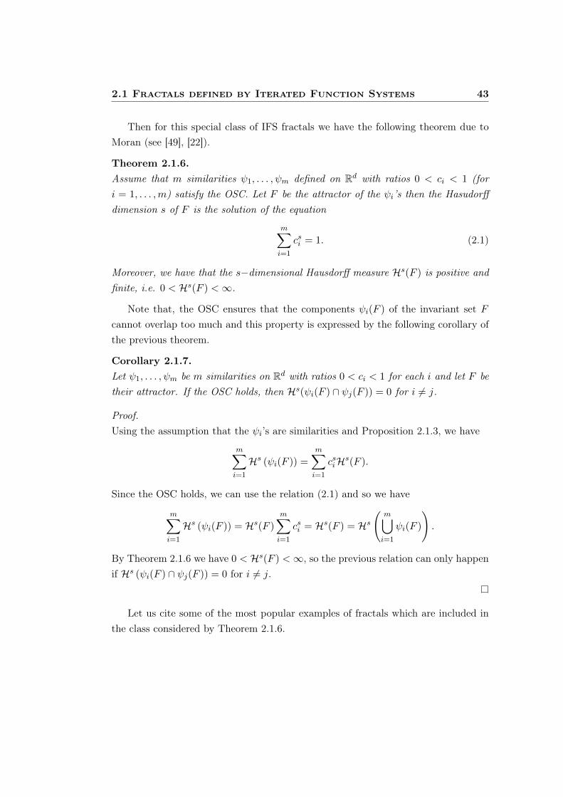
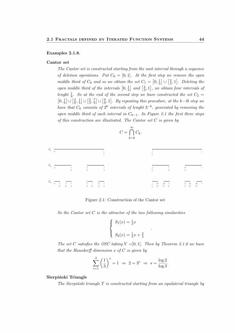
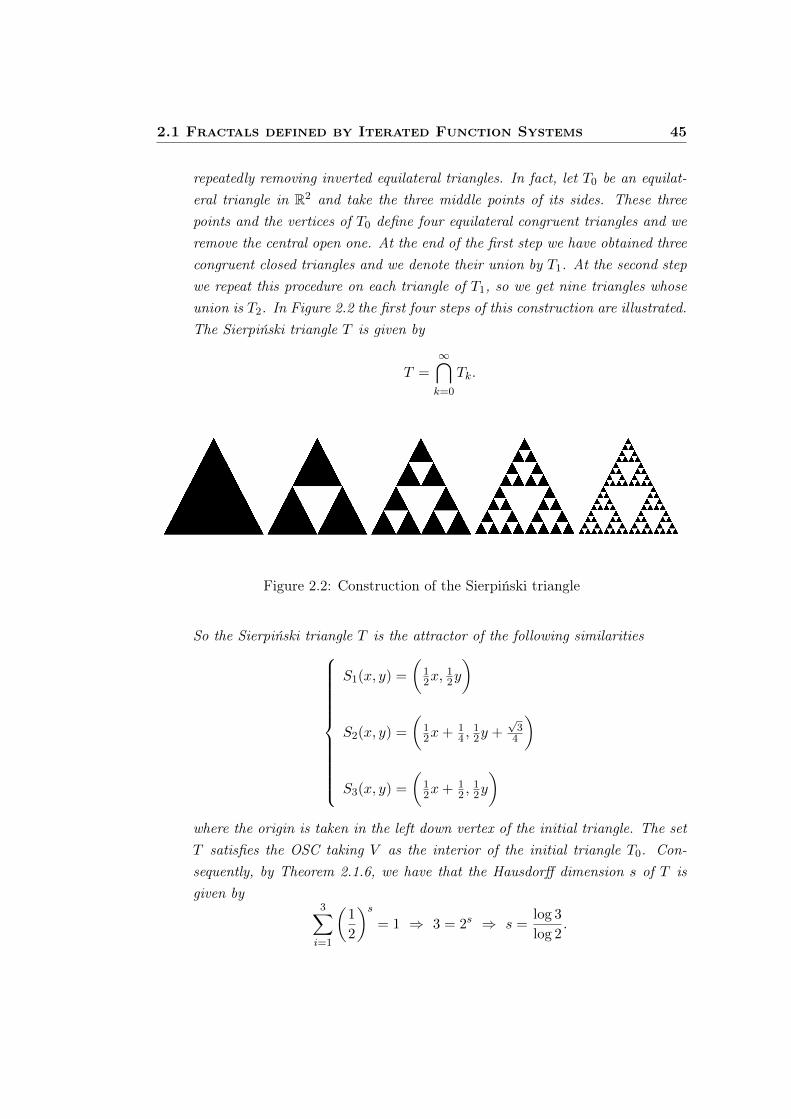
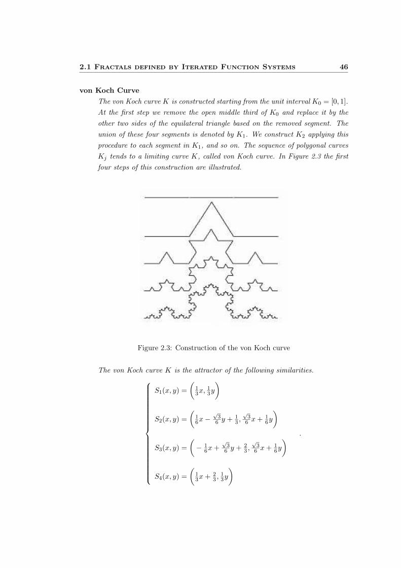
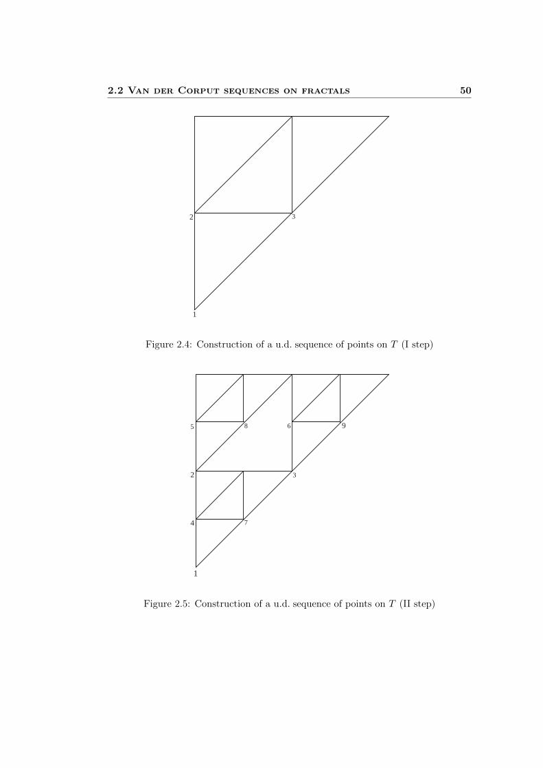
2.1 Construction of the Cantor set . . . . . . . . . . . . . . . . . . . . . . 442.2 Construction of the Sierpiński triangle . . . . . . . . . . . . . . . . . . 452.3 Construction of the von Koch curve . . . . . . . . . . . . . . . . . . . . 462.4 U.d. sequence of points on the Sierpiński triangle (I step) . . . . . . . . 502.5 U.d. sequence of points on the Sierpiński triangle (II step) . . . . . . . 502.6 U.d. sequence of points on the Sierpiński triangle (III step) . . . . . . . 51

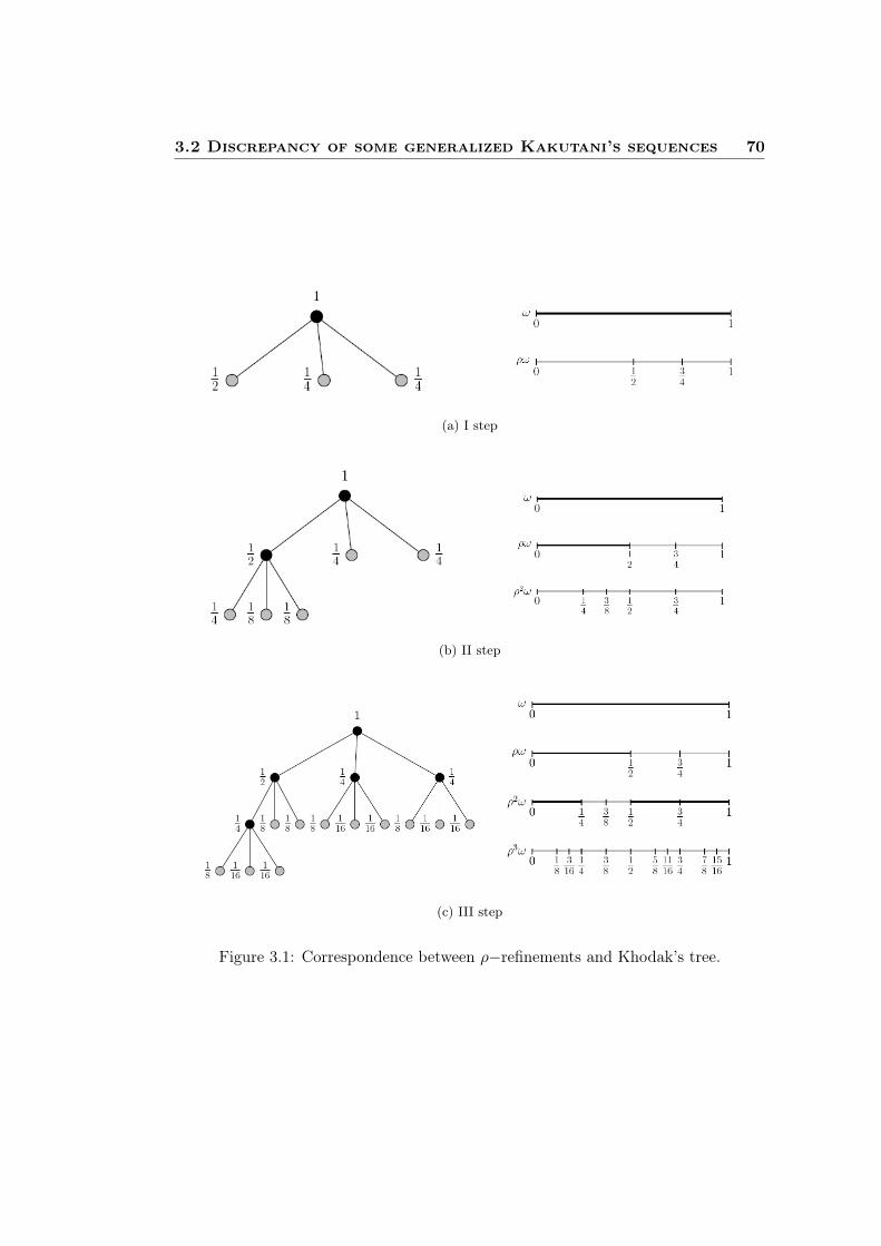
3.1 Correspondence between ρ−refinements and Khodak’s tree. . . . . . . 70

vii

Introduction

The theory of uniform distribution was developed extensively within and amongseveral mathematical disciplines and numerous applications. In fact, the main rootof this theory is number theory and diophantine approximation, but there are strongconnections to various fields of mathematics such as measure theory, probabilitytheory, harmonic analysis, summability theory, discrete mathematics and numericalanalysis.

The central goals of this theory are the assessment of uniform distribution andthe construction of uniformly distributed (u.d.) sequences in various mathematicalspaces. The objectives of this thesis are related to these main topics. In particular,the aim of this work is to introduce new classes of u.d. sequences of points and ofpartitions on [0, 1] and also on fractal sets. Moreover, we intend to present a quanti-tative analysis of the distribution behaviour of the new sequences produced studyingtheir discrepancy.

The problem of finding explicit methods for constructing u.d. sequences wasoriginally investigated in the setting of sequences of points. In fact, the startingpoint of the development of the theory was just the study of u.d. sequences of pointson the unit interval. The result which marked the beginning of the theory was thediscovery that the fractional parts of the multiples of an irrational number are u.d.in the unit interval or, equivalently, on the unit circle. This was a refinement ofan approximation theorem due to Kronecker who had already proved the density ofthis special sequence in the unit interval. So, at the beginning of the last century,many authors independently proposed the theorem about uniform distribution ofKronecker’s sequence such as Bohl [5], Sierpiński [62] and Weyl [70]. The latter wasthe first to estabilish a systematic treatment of uniform distribution theory in hisfamous paper [72], where the formal definition of u.d. sequences of points in [0, 1]

was given for the first time. Moreover, in that paper the theory of u.d. sequences ofpoints was generalized to the higher-dimensional unit cube.

1

INTRODUCTION 2

The uniform distribution of a sequence of points means that the empirical distri-bution of the sequence is asymptotically equal to the uniform distribution. Thereforein the twenties and thirties several authors began to study u.d. sequences of pointsfrom a quantitative point of view introducing the discrepancy [4, 67, 72]. This quan-tity is the classical measure of the deviation of a sequence from the ideal uniformdistribution. Consequently, having a precise estimate of the discrepancy is very use-ful for applications but it is not a trivial problem. Proving general lower bounds forthe discrepancy is a subject still having open questions nowadays.

The interest for u.d. sequences of points, in particular for low discrepancy se-quences, arises from various applications in areas like numerical integration, randomnumber generation, stochastic simulation and approximation theory. Indeed, numer-ical integration was one of the first applications of uniform distribution theory [38].The basic problem considered by numerical integration is to compute an approximatesolution to a definite integral. The classical quadrature formulae are less and less ef-ficient the higher the dimension is. To overcome this problem, a typical approachis trying to approximate the integral of a function f by a weighted average of thefunction evaluated at a set of points {x1, . . . , xN}∫

Idf(x)dx ≈ 1

N

N∑i=1

wif(xi),

where Id is the d−dimensional unit hypercube, the xi’s are N points in Id and

wi > 0 are weights such thatN∑i=1

wi = N . In some cases it is assumed wi = 1 for

every 1 ≤ i ≤ N , as for instance in the classical Monte Carlo method where thepoints x1, . . . , xN are picked from a sequence of random or pseudorandom elementsin Id. The advantage of the Monte Carlo method is that it is less sensitive to theincrease of the dimension.

Another possibility is to use deterministic sequences with given distribution prop-erties for the choice of the xi’s. This procedure is known as Quasi-Monte Carlomethod and it is more advantageous than many other approximation techniques. Infact, the Koksma-Hlawka inequality (1.14) shows that the error of such a methodcan be bounded by the product of a term only depending on the discrepancy of{x1, . . . , xN} and one only depending on the function. Therefore it is convenient tochoose the initial segment of a low discrepancy sequence as the set of integrationpoints in the Quasi-Monte Carlo method. These are sequences with a discrepancyof order (logN)d

N , where d is the dimension of the space in which we take the se-

INTRODUCTION 3

quence. Hence, by using low discrepancy sequences, the Quasi-Monte Carlo methodhas a faster rate of convergence than a corresponding Monte Carlo method, since inthe latter case the point sets do not have necessarily minimal discrepancy. Infact, itbehaves, in average, as 1√

N. Indeed, the Monte Carlo method yields only a probabilis-

tic bound on the integration error. Neverthless, both Monte Carlo and Quasi-MonteCarlo methods offer the advantage to add further points without recalculating thevalues of the function in the previous points and this is a big step forward comparedto classical methods. Quasi-Monte Carlo methods have an important role in finan-cial and actuary mathematics, where high-dimensional integrals occur. During thelast twenty years all these applications have been a rapidly growing area of research[52, 31].

One of the best known techiniques for generating low discrepancy sequences ofpoints in the unit interval was introduced by van der Corput in 1935 (see [66]).Successively, van der Corput’s procedure was extended to the higher-dimensionalcase by Halton [28]. Moreover, a generalization of van der Corput sequences is due toFaure who introduced the permuted or generalized van der Corput sequences. Theyare also very interesting because there exist formulae for the discrepancy of thesesequences which show their good asymptotic behaviour [13, 24, 25].

The study of van der Corput type sequences has not been limited to the classicalsetting of the unit interval in one dimension or the unit hypercube in higher dimen-sions, but interesting extensions have been made to more abstract spaces such asfractals. In fact, the theory of uniform distribution with respect to a given measurehas been generalized in several ways: sequences of points in compact and locally com-pact spaces [45, 51, 32], sequences of probability measures on a separable compactspace [60], in particular sequences of discrete measures associated to partitions of acompact interval [41] and to partitions of a separable metric space [14]. In the follow-ing we use the basic definitions of uniform distribution theory in compact Hausdorffspaces and in a particular class of fractal compact sets.

Fractals are involved in several applications because they are a powerful tool todescribe effectively a variety of phenomena in a large number of fields. To exploitQuasi-Monte Carlo methods on these sets it is essential to study discrepancy boundsfor sequences of points on fractals. One of the earlier papers devoted to uniform dis-tribution on fractals is [27], where this theory is developed on the Sierpiński gasket.In this paper the notion of discrepancy on fractals has been introduced for the first

INTRODUCTION 4

time. The authors define several concepts of discrepancy for sequences of points onthe Sierpiński gasket by choosing different kinds of partitions on this fractal. Succes-sively, these notions were generalized also to other fractals, such as the d−dimensionalSierpiński carpet in [18, 17]. In particular, in [17] a van der Corput type constructionis considered to generate u.d. sequences of points on the d−dimensional Sierpińskicarpet and the exact order of convergence of various notions of discrepancy is deter-mined for these sequences.

In this work we get a more general result by constructing van der Corput type se-quences on a whole class of fractals generated by an Iterated Function System (IFS).More precisely, we are going to study fractals defined by a system of similarities onRd having the same ratio and verifying a natural separation condition of their compo-nents, namely the Open Set Condition (OSC). This class includes the most popularfractals, but also the unit interval [0, 1] which can be seen as the attractor of infinitelymany different IFS. Starting from this remark, which goes back to Mandelbrot [48],we present an alternative construction of the classical van der Corput sequences ofpoints on [0, 1]. By imitating this approach, we introduce an explicit procedure todefine u.d. sequences of points on our special class of fractals (see Subsection 2.2.1).So we call these sequences of van der Corput type, just to emphasize the particularorder given to the points by our algorithm. It is important to underline that as prob-ability on a fractal F of our class we take the normalized s-dimensional Hausdorffmeasure, where s is the Hausdorff dimension of F . This is the most natural choice fora probability measure on this kind of fractals, also because the OSC guarantees theexistence of an easy formula for evaluating the Hausdorff dimension of these fractals(see Theorem 2.1.6). A crucial role in the proof of the uniform distribution of thesequences constructed is played by the elementary sets, i.e. the family of all sets gen-erated by applying our algorithm to the whole fractal F . In this way our techniqueproduces also u.d. sequences of partitions of the fractals belonging to the consideredclass.

The concept of u.d. sequence of partitions on fractals is just one of the mostimportant aspects of this thesis. When we deal with fractals, and in particular withIFS fractals, partitions turn out to be a more convenient tool in relation to theuniform distribution theory. Consequently we extend the notion of u.d. sequences ofpartitions, introduced by Kakutani in 1976 for the unit interval in [41], to our classof fractals.

The construction ideated by Kakutani, called Kakutani’s splitting procedure, al-

INTRODUCTION 5

lows to construct a whole class of u.d. sequences of partitions of [0, 1] and it is basedon the concept of α−refinement of a partition. For a fixed α ∈]0, 1[, the α−refinementof a partition π is obtained by splitting all the intervals of π having maximal lenghtin two parts, proportional to α and 1 − α respectively. Kakutani proved that thesequence of partitions generated through successive α−refinements of the trivial par-tition ω = {[0, 1]} is u.d.. This result received a considerable attention in the lateseventies, when other authors provided different proofs of Kakutani’s theorem [1]and of its stochastic versions, in which the intervals of maximal lenght are splittedaccording to certain probability distributions [68, 46, 47, 8, 55]. Recently differentgeneralizations of Kakutani’s technique have been introduced. A result in this di-rection is the extension of Kakutani’s splitting procedure to the multidimensionalcase with a construction which is intrinsically higher-dimensional [12]. Moreover, ina recent paper of Volčič, Kakutani’s technique is extended also in the one dimen-sional case introducing the concept of ρ−refinement of a partition, which generalizesKakutani’s α−refinement. Actually, the ρ−refinement of a partition π is obtainedby splitting the longest intervals of π into a finite number of parts homothetically toa given finite partition ρ of [0, 1]. The author has proved that the technique of suc-cessive ρ−refinements allows to construct new families of u.d. sequences of partitionsof [0, 1] in [69]. The last paper also investigates the connections of the theory of u.d.sequences of partitions to the well-estabilished theory of u.d. sequences of points,showing how it is possible to associate u.d. sequences of points to any u.d. sequenceof partitions.

Generalized Kakutani’s sequences on [0, 1] are a fundamental tool in the extensionof the results obtained on our class of fractals. The first attempt of enlarging the classof fractals considered in our previous analysis consists in eliminating the restrictionthat all the similarities defining the fractal have the same ratio.

The procedure of successive ρ-refinements fits perfectly to the problem of gener-ating u.d. sequences of partitions on this new class of fractals. Let ψ = {ψ1, . . . , ψm}be a system of m similarities on Rd having ratio c1, . . . , cm ∈ ]0, 1[ respectively andsuch that they verify the OSC. Let F be the attractor of ψ and let s be its Hausdorffdimension. Applying successively the m similarities to the fractal F , we get a firstpartition consisting of m subsets of F each of probability pi = csi (where for probabil-ity we again mean the normalized s−dimensional Hausdorff measure). At the secondstep we choose the susbsets with the highest probability and we apply to each ofthem the m similarities in the same order, and so on. Iterating this procedure, which

INTRODUCTION 6

exploits the same basic idea of ρ−refinements, we obtain a sequence of partitions ofF . Now the problem is the assessment of the uniform distribution of these sequencesand the estimation of their discrepancy.

According to the Mandelbrot’s remark the simplest setting for this problem isthe unit interval. In fact, if we consider [0, 1] as the attractor of m similaritiesϕ1, . . . , ϕm having different ratios and satisfying the OSC and we apply the pro-cedure described above, then we get exactly the sequence of ρ−refinements (ρnω),where ρ = {ϕ1([0, 1]), . . . , ϕm([0, 1])} and ω = {[0, 1]}.

In the second part of this work we focus on deriving bounds for the discrepancyof the generalized Kakutani’s sequences of partitions of [0, 1] generated through thetechinique of successive ρ−refinements. The problem of estimating the asymptoticbehaviour of the discrepancy of these sequences has been posed for the first time in[69]. At the moment the only known discrepancy bounds for a class of such sequenceshave been given by Carbone in [10]. In this paper the author considered the so-calledLS-sequences which are generated by successive ρ−refinements where ρ is a partitionwith L subintervals of [0, 1] of length α and S subintervals of length α2 (where α isgiven by the equation Lα+ Sα2 = 1).

To study this problem in more generality we use a correspondence between theprocedure of successive ρ−refinements and Khodak’s algorithm [43]. This new ap-proach is based on a parsing tree related to Khodak’s coding algorithm, which rep-resents the successive ρ-refinements. We introduce improvements of the results ob-tained in [20] to provide significative bounds of the discrepancy for all the sequencesgenerated by successive ρ−refinements, when ρ is a partition of [0, 1] consisting ofm subintervals of lenghts p1, . . . , pm such that log

(1p1

), . . . , log

(1pm

)are rationally

related. This result applies also to a countable family of classical Kakutani’s se-quences and provides, for the first time after thirty years, quantitative estimates oftheir discrepancy. Moreover, the class of generalized Kakutani’s sequences belongingto this rational case also includes the LS−sequences.

In the following we are also able to cover several situations in the irrational case,which means that at least one of the fractions log pi

log pjis irrational. This case is much

more involved than the rational one. In this work we discuss some instances ofthe irrational case when the initial probabilities are two, namely p and q = 1 − p.The upper bounds for the discrepancy that we obtain in this subcase are weaker,since they depend heavily on Diophantine approximation properties of the ratio log p

log q .Furthermore, if the initial partition is composed of more than two intervals, then the

INTRODUCTION 7

analysis of the behaviour of the discrepancy is even more complicated, as evident bycomparing with [26].

The approach applied for achieving these bounds of the discrepancy of general-ized Kakutani’s sequences on [0, 1] can be also used for the sequences of partitionsconstructed on fractals defined by similarities which do not have the same ratio andsatisfing the OSC. In fact, we have described above an analogue of the method ofsuccessive ρ−refinements which allows to produce sequences of partitions on this newclass of fractals. We actually introduce a new correspondence between nodes of thetree associated to Khodak’s algorithm and the subsets belonging to the partitionsgenerated on the fractal. Consequently, with a technique similar to the one used on[0, 1] we prove bounds for the elementary discrepancy of these sequences of partitions,too.

Let us give a brief outline of the thesis.Chapter 1 provides the basic background knowledge on the areas of uniform

distribution theory that are investigated in this thesis. The first part of the chapterdeals with the classical part of the theory. Basic definitions and properties of u.d.sequences of points on the unit interval are introduced and specific examples of u.d.sequences of points are described throughout. Then a whole section is devoted tothe more recent theory of u.d. sequences of partitions, which plays an essential rolein this work. Some extensions of uniform distribution theory are also touched on inthis chapter, such as the theory in the unit hypercube and the theory in Hausdorffcompact spaces.

Chapter 2 regards the uniform distribution on a special class of fractals. Moreprecisely, we are concerned with fractals generated by an iterated function system ofsimilarities having the same ratio and satisfying the open set condition. We proposean algorithm for generating u.d. sequences of partitions and of points on this classof fractals. Furthermore, in the last part of this chapter we study the order ofconvergence of the elementary discrepancy of the van der Corput type sequencesconstructed on these fractals. The results presented in this chapter have been firstpublished in [40].

In Chapter 3 we extend the results given in the second chapter to a wider classof fractals by using a new approach, which allows to derive bounds for the discrep-ancy of a class of generalized Kakutani’s sequences of partitions of [0, 1], constructedthrough successive ρ−refinements. We present the recent technique of ρ−refinementsand the generalization of Kakutani’s theorem to the class of sequences of partitions

INTRODUCTION 8

generated by this procedure. Then, we analyze the behaviour of the discrepancy ofthese sequences from a new point of view. The crucial idea is a tree representationof any sequence of partitions constructed by successive ρ−refinements, which is pre-cisely the parsing tree generated by Khodak’s coding algorithm. The correspondencebetween the two techniques allows not only to give optimal upper bounds in theso-called rational case on [0, 1] but also to extend the results obtained in the secondchapter to a wider class of fractals. Moreover, we study the irrational case which ismore involved than the rational one. Finally, we give some examples and applicationsof the results achieved so far. The new contributions presented in this chapter arecollected in [19].

The thesis concludes by reviewing, in Chapter 4, the main results we haveobtained and indicating open problems and directions of future research.

Chapter 1

Preliminary topics

This chapter is meant to give a short overview of known results about uniformdistribution theory not only in the classical setting of [0, 1] but also in more generalspaces. First we intend to mention some necessary definitions and basic resultsconcerning u.d. sequences of points in [0, 1]. Then we will introduce the more recenttheory of u.d. sequences of partitions which is fundamental in the development ofthis work. Finally, we will point out the main aspects of uniform distribution theoryon the unit hypercube and on compact spaces.

1.1 Uniformly distributed sequences of points in [0, 1]

In this section we develop the classical part of uniform distribution theory. Thestandard references for this topic are [45] and [21]. We start introducing the basicconcepts related to u.d. sequences of points and then we proceed to consider thequantitative aspect of the theory. Moreover, a whole subsection is devoted to aspecial class of sequences with certain advantageous distribution properties, namelythe van der Corput sequences.

1.1.1 Definitions and basic properties

First of all, let us state the main definition of the theory.

Definition 1.1.1.A sequence (xn) of points in [0, 1] is said to be uniformly distributed (u.d.) if for anyreal number a such that 0 < a ≤ 1 we have

limN→∞

1

N

N∑n=1

χ[0,a[(xn) = a (1.1)

9

1.1 Uniformly distributed sequences of points in [0, 1] 10

where χ[0,a[ is the characteristic function of the interval [0, a[.

Let us introduce some concepts which are very useful to characterize u.d. se-quences of points.

Definition 1.1.2.A class F of Riemann-integrable functions on [0, 1] is said to be determining forthe uniform distribution of sequences of points, if for any sequence (xn) in [0, 1] thevalidity of the relation

limN→∞

1

N

N∑n=1

f(xn) =

∫ 1

0f(x) dx (1.2)

for all f ∈ F already implies that (xn) is u.d.. In particular, a system of subsetsof [0, 1] such that the family of their characteristic functions is determining is calleddiscrepancy system.

Hence, we can restate the Definition 1.1.1 saying that the family of all character-istic functions χ[0,a[ for 0 < a ≤ 1 is determining or that the system of all sets [0, a[

for 0 < a ≤ 1 is a discrepancy system.An important determining class is the family of all continuous (real or complex-

valued) functions on [0, 1]. This result is due to Weyl and it is very useful to extendthe theory to more general spaces [71, 72].

Theorem 1.1.3 (Weyl’s Theorem).A sequence (xn) of points in [0, 1] is u.d. if and only if for any real-valued continuousfunction f defined on [0, 1] the equation (1.2) holds.

Proof.Let (xn) be u.d. and let f be a step function

f(x) =k−1∑i=0

ciχ[ai,ai+1[(x) (1.3)

where 0 = a0 < a1 < . . . < ak = 1 and ci ∈ R for i = 0, . . . , k − 1. Then it follows


from (1.1) and (1.3) that

limN→∞

1

N

N∑n=1

f(xn) = limN→∞

1

N

N∑n=1

k−1∑i=0

ciχ[ai,ai+1[(xn)

=k−1∑i=0

ci limN→∞

1

N

(N∑n=1

χ[0,ai+1[(xn)−N∑n=1

χ[0,ai[(xn)

)

=

k−1∑i=0

ci

(∫ 1

0χ[0,ai+1[(x) dx−

∫ 1

0χ[0,ai[(x) dx

)

=k−1∑i=0

∫ 1

0ciχ[ai,ai+1[(x) dx

=

∫ 1

0f(x) dx.

Now, assume that f is a real-valued function defined on [0, 1]. Fixed ε > 0, by thedefinition of the Riemann integral, there exist two step functions f1 and f2 such that

f1(x) ≤ f(x) ≤ f2(x) , ∀x ∈ [0, 1]

and ∫ 1

0(f2(x)− f1(x)) dx ≤ ε.

Then we have the following chain of inequalities∫ 1

0f(x) dx− ε ≤

∫ 1

0f2(x) dx− ε ≤

∫ 1

0f1(x) dx = lim

N→∞

1

N

N∑n=1

f1(xn)

≤ lim infN→∞

1

N

N∑n=1

f(xn) ≤ lim supN→∞

1

N

N∑n=1

f(xn)

≤ limN→∞

1

N

N∑n=1

f2(xn) =

∫ 1

0f2(x) dx

≤∫ 1

0f1(x) dx+ ε ≤

∫ 1

0f(x) dx+ ε.

So the relation (1.2) holds for all continuous functions on [0, 1].Conversely, let (xn) be a sequence of points in [0, 1] such that the (1.2) holds for

every real-valued continuous function f defined on [0, 1]. Let a ∈]0, 1[, then for anyε > 0 there exist two continuous functions g1 and g2 such that

g1(x) ≤ χ[0,a[(x) ≤ g2(x) , ∀x ∈ [0, 1]


and ∫ 1

0(g2(x)− g1(x)) dx ≤ ε.

Then we have

a− ε ≤∫ 1

0g2(x) dx− ε ≤

∫ 1

0g1(x) dx = lim

N→∞

1

N

N∑n=1

g1(xn)

≤ lim infN→∞

1

N

N∑n=1

χ[0,a[(xn) ≤ lim supN→∞

1

N

N∑n=1

χ[0,a[(xn)

≤ limN→∞

1

N

N∑n=1

g2(xn) =

∫ 1

0g2(x) dx

≤∫ 1

0g1(x) dx+ ε ≤ a+ ε.

Since ε is arbitrarily small, we have (1.1).

Moreover, we can state a more general result.

Theorem 1.1.4.A sequence (xn) of points in [0, 1] is u.d. if and only if for any Riemann-integrablefunction f defined on [0, 1] the equation (1.2) holds.

Proof.The sufficiency follows directly from the previous theorem, because every continuousfunction is Riemann-integrable. The other implication was shown by De Bruijn and

Post [9], who proved that if f is defined on [0, 1] and if the averages 1N

N∑n=1

f(xn)

admit limit for any (xn) u.d., then f is Riemann-integrable.

The problem of finding the largest reasonable determining classes has been ad-dressed also in [14] and [57].

Other examples of determing classes are the following ones.

Examples

• The class of all characteristic functions of open (closed or half-open) subinter-vals of [0, 1] is determining.


• The class of the characteristic functions of all intervals of the type [0, q] withq ∈ Q is determining.

• The class of all step functions, i.e. functions given by finite linear combinationsof characteristic functions of half-open subintervals of [0, 1] is determining.

• The class of all continuous (real or complex-valued) functions g on [0, 1] suchthat g(0) = g(1) is determining.

• The class of all polynomials with rational coefficients is determining.

Now, consider all functions of the type f(x) = e2πihx where h is a non-zero integer.One of the most important facts of uniform distribution theory is that these functionsgive a criterion to determine if a sequence of points is u.d..

Theorem 1.1.5 (Weyl’s Criterion).The sequence (xn) is u.d. if and only if

limN→∞

1

N

N∑n=1

e2πihxn = 0

for all integers h 6= 0.

This important result was proved for the first time by Weyl in [72], but a lot ofproofs can be find in literature. Moreover, this criterion has a variety of applicationsin uniform distribution theory and also in the estimation of exponential sums. In par-ticular, Weyl applied this theorem to the special sequence ({nθ}), with θ irrational,to give a new proof of the following theorem.

Let us recall that for any x ∈ R, we denote by {x} the fractional part of x, whichsatisfies {x} = x− [x], where [x] is the integral part of x (i.e the greatest integer lessor equal to x).

Theorem 1.1.6.Let θ be an irrational number. Then the sequence ({nθ}) is u.d..

This result was independently estabilished byWeyl [70], Bohl [5] and Sierpiński [62]in 1909-1910. The problem of the distribution of this special sequence has its originin the theory of secular perturbations in astronomy and signs the beginning of thetheory of u.d. sequences of points. Theorem 1.1.6 improves a previous theorem dueto Kronecker, who proved that the points einθ are dense in the unit circle, wheneverθ is an irrational multiple of π (Kronecker’s approximation theorem). For this reasonthe sequence ({nθ}) with θ irrational is called Kronecker’s sequence.


Finally, it is important to underline that uniform distribution has also a measure-theoretic aspect. In fact, if we look at Definition 1.1.1, we realize that a sequence (xn)

of points in [0, 1] is u.d. if and only if the sequence of discrete measures(

1n

n∑i=1

δxi

)converges weakly to the Lebesgue measure λ on [0, 1], where δt is the Dirac measureconcentrated in t.

The notion of weak convergence of measures represents the link between u.d.sequence of points and u.d. sequence of partitions.

1.1.2 Discrepancy of sequences

As a quantitative measure of the distribution behaviour of a u.d. sequence weconsider the so-called discrepancy, that is the maximal deviation between the em-pirical distribution of the sequence and the uniform distribution. This notion wasstudied for the first time in a paper of Bergström, who used the term “Intensität-dispersion”(see [4]). The term discrepancy was probably coined by van der Corput.Moreover, the first intensive study of discrepancy is due to van der Corput and Pisotin [67].

Definition 1.1.7 (Discrepancy).Let ωN = {x1, . . . , xN} be a finite set of real numbers in [0, 1]. The number

DN (ωN ) = sup0≤a<b≤1

∣∣∣∣∣ 1

N

N∑i=1

χ[a,b[(xi)− (b− a)

∣∣∣∣∣is called the discrepancy of the given set ωN .

If (xn) is an infinite sequence of points, we associate to it the sequence of positivereal numbers DN ({x1, x2, . . . xN}). So, the symbol DN (xn) denotes the discrepancyof the initial segment {x1, x2, . . . xN} of the infinite sequence.

The importance of the concept of discrepancy in uniform distribution theory isrevealed by the following fact (see [72] for more details).

Theorem 1.1.8.A sequence (xn) of points in [0, 1] is u.d. if and only if

limN→∞

DN (xn) = 0.

Sometimes it is useful to restrict the family of intervals considered in the definitionof discrepancy. The most important type of restriction is to consider only intervalsof the form [0, a[ with 0 < a ≤ 1.


Definition 1.1.9 (Star discrepancy).Let ωN = {x1, . . . , xN} be a finite set of real numbers in [0, 1], we define star dis-crepancy of ωN the quantity

D∗N (ωN ) = sup0<a≤1

∣∣∣∣∣ 1

N

N∑i=1

χ[0,a[(xi)− a

∣∣∣∣∣.The definition D∗N is extended to the infinite sequence in the same way as we

did for DN . Moreover, the discrepancy and the star discrepancy are related by thefollowing inequality.

Theorem 1.1.10.For any sequence (xn) of points in [0, 1] we have

D∗N (xn) ≤ DN (xn) ≤ 2D∗N (xn).

The most prominent open problem in theory of irregularities of distribution is todetermine the optimal lower bound for the discrepancy. A first trivial lower boundis given by the following proposition.

Proposition 1.1.11.For any finite set ω = {x1, . . . , xN} in [0, 1] we have that

1

N≤ DN (ω) ≤ 1.

The finite set xn = nN , n = 1, . . . , N satisfies DN ({x1, . . . , xN}) = 1

N . Butsequences of this kind can only exist in the one-dimensional case by a theorem due toRoth [56] and this shows that the lower bound is optimal. Moreover, in this exampleit is easy to see that for every N a new set {x1, . . . , xN} is constructed. So the naturalquestion is if there exists an infinite sequence (xn) in [0, 1] such thatDN (xn) = O

(1N

)as N →∞. Van der Corput made the conjecture that there are no sequences of thiskind in the unit interval and this was proved by van Aardenne-Ehrenfest in [64, 65].But the van der Corput conjecture was completely solved also from a quantitativepoint of view with the following important result due to Schmidt [61].

Theorem 1.1.12 (Schmidt’s Theorem).For any sequence (xn) in [0, 1] we have that

NDN (xn) > c logN

for infinitely many positive integers N , where c > 0 is an absolute constant.


This lower bound is the best possible in the one-dimensional case.

Usually, sequences having discrepancy of the order O(

logNN

)are called low dis-

crepancy sequences and they are very important for several applications. An inter-esting example of this kind of sequences are the van der Corput sequences.

1.1.3 The van der Corput sequence

In 1935 van der Corput introduced a procedure to generate low discrepancy se-quences on [0, 1] (see [66]). These sequences are considered the best distributed on[0, 1], because no infinite sequence has yet been found with discrepancy of smallerorder of magnitude than the van der Corput sequences. The technique of van derCorput is based on a very simple idea. First of all we have to define the radicalinverse function which is at the basis of this construction.

Definition 1.1.13 (Radical-inverse function).

Let b ≥ 2 an integer and let n =r∑

k=0

akbk be the digital expansion of the integer n ≥ 1

in base b, ak ∈ {0, . . . , b− 1}. The function

γb(n) =

r∑k=0

akb−k−1

is called radical inverse function in base b.

The radical inverse function γb(n) represents the fraction lying between 0 and 1

constructed by reversing the order of the digits in the b−adic expansion of n.

Definition 1.1.14 (van der Corput sequences).Let b ≥ 2 a fixed prime integer. The sequence (xn)n≥1, where

xn = γb(n− 1),

is called van der Corput sequence in base b.

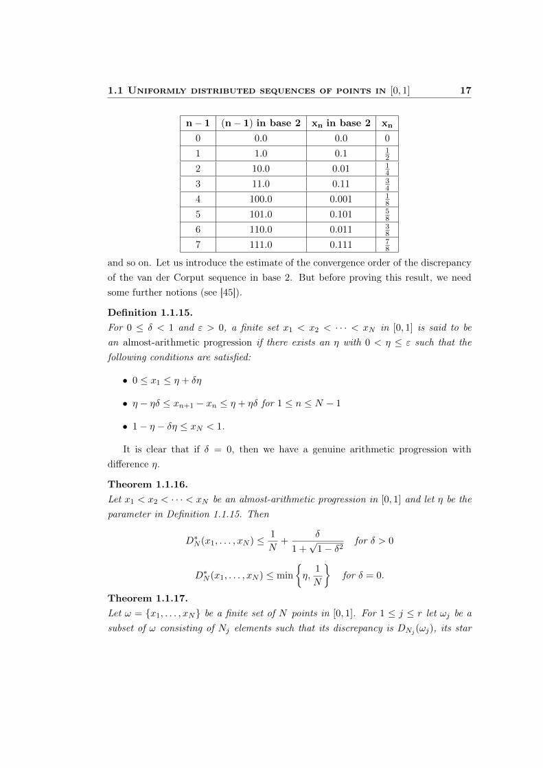
For example, the van der Corput sequence in base b = 2 is given by

0,1

2,

1

4,

3

4,

1

8,

5

8,

3

8,

7

8, . . .

The construction of these points is explicitely showed in the following table.


n− 1 (n− 1) in base 2 xn in base 2 xn

0 0.0 0.0 01 1.0 0.1 1

2

2 10.0 0.01 14

3 11.0 0.11 34

4 100.0 0.001 18

5 101.0 0.101 58

6 110.0 0.011 38

7 111.0 0.111 78

and so on. Let us introduce the estimate of the convergence order of the discrepancyof the van der Corput sequence in base 2. But before proving this result, we needsome further notions (see [45]).

Definition 1.1.15.For 0 ≤ δ < 1 and ε > 0, a finite set x1 < x2 < · · · < xN in [0, 1] is said to bean almost-arithmetic progression if there exists an η with 0 < η ≤ ε such that thefollowing conditions are satisfied:

• 0 ≤ x1 ≤ η + δη

• η − ηδ ≤ xn+1 − xn ≤ η + ηδ for 1 ≤ n ≤ N − 1

• 1− η − δη ≤ xN < 1.

It is clear that if δ = 0, then we have a genuine arithmetic progression withdifference η.

Theorem 1.1.16.Let x1 < x2 < · · · < xN be an almost-arithmetic progression in [0, 1] and let η be theparameter in Definition 1.1.15. Then

D∗N (x1, . . . , xN ) ≤ 1

N+

δ

1 +√

1− δ2for δ > 0

D∗N (x1, . . . , xN ) ≤ min

{η,

1

N

}for δ = 0.

Theorem 1.1.17.Let ω = {x1, . . . , xN} be a finite set of N points in [0, 1]. For 1 ≤ j ≤ r let ωj be asubset of ω consisting of Nj elements such that its discrepancy is DNj (ωj), its star


discrepancy is D∗Nj (ωj), ωj ∩ ωi = ∅ for all j 6= i and N = N1 + . . .+Nr. Then

DN (ω) ≤r∑j=1

Nj

NDNj (ωj)

and also

D∗N (ω) ≤r∑j=1

Nj

ND∗Nj (ωj).

Now, we are ready to prove the following result.

Theorem 1.1.18.The discrepancy DN (xn) of the van der Corput sequence in base 2 satisfies

DN (xn) ≤ c(

log(N + 1)

N

)where c > 0 is an absolute constant.

Proof.Let N ≥ 1. We represent N by its dyadic expansion

N = 2h1 + . . .+ 2hr with h1 > h2 > . . . > hr ≥ 0.

Partition the interval [1, N ]∩N of integers in r subsetsM1, . . . ,Mr defined as follows

Mj = [2h1 + . . .+ 2hj−1 + 1, 2h1 + . . .+ 2hj−1 + 2hj ] ∩ N for 1 < j ≤ r

and put M1 = [0, 2h1 ] ∩ N.An integer n ∈Mj can be written in the form

n = 1 + 2h1 + . . .+ 2hj−1 +

hj−1∑i=0

ai2i, with ai ∈ {0, 1}.

In fact, we get all 2hj integers in Mj if we let the aj run through all the possiblecombinations of 0 and 1. It follows that the point xn of the van der Corput sequenceis given by

xn = 2−h1−1 + . . .+ 2−hj−1−1 +

hj−1∑i=0

ai2−i−1 = yj +

hj−1∑i=0

ai2−i−1

where yj only depends on j and not on n.

If n runs through Mj , then the sumhj−1∑i=0

ai2−i−1 runs through all fractions

0, 2−hj , . . . , (2hj − 1) · 2−hj . Moreover, we can note that 0 ≤ yj < 2−hj .

1.2 Uniformly distributed sequences of partitions on [0, 1] 19

We conclude that if the elements xn with n ∈ Mj are ordered according to theirmagnitude, then we obtain a sequence ωj consisting of Nj = 2hj elements that is anarithmetic progression with parameters δ = 0 and η = 2−hj , (see Definition 1.1.15).By Theorem 1.1.16, we have that

D∗Nj (ωj) ≤ min

{η,

1

Nj

}= 2−hj .

The set of the firstN terms of the van der Corput sequence, i.e. ω = {x1, . . . , xN},can be decomposed in the r subset ωj defined above, since N = N1 + · · · + Nr =

2h1 + . . .+ 2hr . Hence, by Theorem 1.1.17 we have

D∗N (ω) ≤r∑j=1

Nj

ND∗Nj (ωj) ≤

r∑j=1

1

N=

r

N. (1.4)

It remains to estimate r in terms of N . Since h1 > h2 > . . . > hr ≥ 0 then wehave that hr ≥ 0 , hr−1 ≥ 1 , hr−2 ≥ 2, . . . , h1 ≥ r − 1. So we have that

N = 2h1 + . . .+ 2hr ≥ 2r−1 + . . .+ 20 = 2r − 1,

and sor ≤ log(N + 1)

log 2. (1.5)

Finally, by combining (1.4) and (1.5) we have

D∗N (ω) ≤ log(N + 1)

N log 2

and since Theorem 1.1.10 holds, we have

DN (ω) ≤(

2

log 2

)·(

log(N + 1)

N

).

1.2 Uniformly distributed sequences of partitions on [0, 1]

In this section, we will consider u.d. sequences of partitions of [0, 1], a conceptwhich has been introduced in 1976 by Kakutani in [41]. In particular, we will sketchthe theory of u.d. sequences of partitions introducing the significant example con-structed by Kakutani. In the second part of this section, we will investigate therelation between u.d. sequences of partitions and u.d. sequences of points. This topicis analyzed more thoroughly in [69].

Firstly, let us give the basic definitions.


Definition 1.2.1.Let (πn) be a sequence of partitions of [0, 1], where πn = {[tni−1, t

ni ] : 1 ≤ i ≤ k(n)}.

The sequence (πn) is said to be uniformly distributed (u.d.) if for any continuousfunction f on [0, 1] we have

limn→∞

1

k(n)

k(n)∑i=1

f(tni ) =

∫ 1

0f(t) dt. (1.6)

Equivalently, (πn) is u.d. if the sequence of discrepancies

Dn = sup0≤a<b≤1

∣∣∣∣ 1

k(n)

k(n)∑i=1

χ[a,b[(t(n)i )− (b− a)

∣∣∣∣ (1.7)

tends to 0 as n→∞.Similarly to the sequences of points, we can note that the uniform distribution

of the sequence of partitions (πn) is equivalent to the weak convergence to λ of theassociated sequences of measures (νn), with

νn =1

k(n)

k(n)∑i=1

δtni . (1.8)

Moreover, it is easy to see that the uniform distribution of the sequence of parti-tions (πn) is equivalent to each of the following two conditions:

1. For any choice of the points τni ∈ [tni−1, tni ] we have

limn→∞

1

k(n)

k(n)∑i=1

f(τni ) =

∫ 1

0f(t) dt

for any continuous function f on [0, 1].

2. For any choice of the points τni ∈ [tni−1, tni ] we have that the sequence of measures

1

k(n)

k(n)∑i=1

δτni

converges weakly to the Lebesgue measure λ on [0, 1].

1.2.1 Kakutani’s splitting procedure

Let us describe a particular technique which allows to construct a whole class ofu.d. sequences of partitions of [0, 1]. This procedure was introduced by Kakutani in1976 and works through successive α−refinements of the unit interval [41].


Definition 1.2.2.If α ∈]0, 1[ and π = {[ti−1, ti] : 1 ≤ i ≤ k} is any partition of [0, 1], then Kakutani’sα-refinement of π (which will be denoted by απ) is obtained by splitting only theintervals of π having maximal lenght in two parts, proportional to α and β = 1 − αrespectively.

We will denote by α2π the α-refinement of απ and, in general, by αnπ theα−refinement of αn−1π. Starting with the trivial partition ω of [0, 1], i.e. ω = {[0, 1]},we get Kakutani’s sequence of partitions κn = αnω.

For example, if α < β we have thatκ1 = {[0, α], [α, 1]}κ2 = {[0, α], [α, α+ αβ], [α+ αβ, 1]}and so on.

About this splitting procedure Kakutani proved the following result.

Theorem 1.2.3.For every α ∈]0, 1[ the sequence of partitions (κn) of [0, 1] is u.d..

The most transparent proof of this theorem is due to Adler and Flatto and followsfrom a combination of classical results from ergodic theory [1]. Indeed, Kakutani’sprocedure caught the attention of several authors in the late seventies also from astochastic point of view. In fact, Kakutani’s theorem was a partial answer to thefollowing question posed by the physicist H. Araki, which regarded random splittingof the interval [0, 1]. Let X1 be choosen randomly with respect to the uniform distri-bution on [0, 1]. Once X1, . . . , Xn have been choosen, let Xn+1 be a point picked atrandom and accordingly to the uniform distribution in the largest of the n+1 intervalsdetermined by the previous n points. Kakutani had been originally asked whetherthe associated sequence of empirical distribution functions converges uniformly, withprobability 1, to the distribution function of the uniform random variable on [0, 1].

This question has been studied in [68, 46, 47, 8] and later in [55]. It is importantto note that in the probabilistic setting the possibility that the partition obtained atthe n−th step has more than one interval of maximal lenght can be neglected, sinceit is an event which has probability equal to zero. On the other hand, in Kakutani’ssplitting procedure for every α the partition αnω has more than one interval ofmaximal lenght for infinitely many values of n.

Recently, some new results and ideas revived the interest for this subject. In fact,Kakutani’s technique has been generalized in several directions. In [12] the splittingprocedure has been extended to higher dimensions, providing a sequence of nodes in


the hypercube [0, 1]d which is proved to be u.d.. In [11] a von Neumann type theoremis presented for sequences of partitions of [0, 1]. More precisely, u.d. sequences ofpartitions of the unit interval are constructed starting from sequences of partitionsπn whose diameter tends to zero for n→∞. In [69] the concept of α−refinement isgeneralized and it is introduced a new splitting procedure for constructing a largerclass of u.d. sequences of partitions on [0, 1]. Moreover, in this paper it is analyzed thedeep relation between the theory of u.d. sequences of partitions and the theory of u.d.sequences of points. This strong connection between the two theories makes moreinteresting the study of u.d. sequences of partitions in view of possible applicationsto Quasi-Monte Carlo methods.

1.2.2 Associated uniformly distributed sequences of points

In the following, we intend to study the problem of associating to a u.d. sequenceof partitions a u.d. sequence of points. Before investigating this problem, let us notethat the converse problem results to be easier in many cases.

Theorem 1.2.4.If (xn) is a u.d. sequence of points in [0, 1] such that xn 6= xm when n 6= m andxn /∈ {0, 1} for any n ∈ N, then the sequence of partitions (πn), where each πn isdetermined by the points {0, 1, xk with k ≤ n} ordered by magnitude, is u.d..

Proof.By using the assumption that (xn) is u.d. and Theorem 1.1.3, it follows that therelation (1.6) holds for any continuous function f defined on [0, 1].

The requirement that xn 6= xm when n 6= m is important and it is not possibleto avoid this assumption in the theorem as it is shown in the following example.

ExampleConsider the sequence (xn) defined by consecutive blocks of 4m points for m ∈ N.Each block is defined as follows{

1

2m+ 1,

1

2m+ 1, . . . ,

m

2m+ 1,

m

2m+ 1, . . . ,

1

2,2m+ 1

4m,2m+ 2

4m, . . . ,

4m− 1

4m

}.

In each block the first m points are repeated twice, while the others are all distinct.In this way, the points of the sequence have double density in the right half of[0, 1], but they have however a good distribution because of the repetition in the left


half of [0, 1]. So the sequence (xn) is u.d.. But when we take in consideration thesequence of partitions (πn) associated to (xn), according to the procedure describedin the previous theorem, the repetitions are cancelled. Hence, we get a sequence (πn)

having twice as many subintervals in[

12 , 1]than in

[0, 1

2

[and so (πn) is not u.d..

Now, consider our starting problem of associating a u.d. sequence of points to a fixedu.d. sequence of partitions. Let us introduce an important result proved by Volčič in[69], where a probabilistic answer to this problem is given.

Suppose (πn) is a u.d. sequence of partitions in [0, 1] with πn = {[tni−1, tni ] : 1 ≤

i ≤ k(n)}. The natural question is if it is possible to rearrange the points tni deter-mining the partitions πn, for 1 ≤ i ≤ k(n), in order to get a u.d. sequence of points.Clearly, there exist many ways of reordering the points tni . A natural restriction isthat we first reorder all the points determining π1 then those defining π2, and so on.This kind of reorderings are called sequential reorderings.

Before presenting the result of Volčič, we need some preliminaries. In particular,we introduce a version of the strong law of large numbers for negatively correlatedrandom variables, which is attributed to Aleksander Rajchman and can be provedfollowing the lines of Theorem 5.1.2 in [16].

Lemma 1.2.5.Let (ϕn) be a sequence of real, negatively correlated random variables with variancesuniformly bounded by V on the probability space (W,P ). Moreover, suppose that

limi→∞

E(ϕi) = M.

Then

limn→∞

1

n

n∑i=1

ϕi = M almost surely.

Proof.We may assume E(ϕi) = 0 and remove afterwards this restriction by applying theconclusions to the sequence of random variables ϕi − E(ϕi).


Put Sn =n∑i=1

ϕi. For any ε > 0, by using the Čebišev inequality we have

P

(1

n2Sn2 ≥ ε

)≤ 1

ε2V ar

(1

n2Sn2

)=

1

n4ε2E(S2n2

)=

1

n4ε2E

n2∑i=1

ϕi

2

=1

n4ε2E

n2∑i=1

ϕ2i +

n2∑i=1

n2∑i 6=jj=1

ϕiϕj

=1

n4ε2

n2∑i=1

E(ϕ2i

)+

n2∑i=1

n2∑i 6=jj=1

E (ϕiϕj)

.

Now, because of the negative correlation of the ϕi’s we have that the terms E (ϕiϕj)

for i 6= j are not positive. So by using this fact and the bound for the variance, weget the estimate

P

(1

n2Sn2 ≥ ε

)≤ 1

n4ε2

n2∑i=1

E(ϕ2i

) =1

n4ε2

n2∑i=1

V ar (ϕi)

≤ V

n2ε2.

Since the series of the upper bounds is convergent, the series

∞∑n=1

P

(1

n2Sn2 ≥ ε

)is convergent, too. Therefore by the Borel-Cantelli lemma, we have that

limn→∞

1

n2Sn2 = 0 a.s.. (1.9)

Define nowLn = max

n2≤j<(n+1)2|Sj − Sn2 | .


For the same ε, the Čebišev inequality implies that

P

(Lnn2≥ ε)≤ 1

n4ε2E(L2n

)≤ 1

n4ε2E

(n+1)2−1∑j=n2+1

|Sj − Sn2 |2

=1

n4ε2E

(n+1)2−1∑j=n2+1

j∑i=n2+1

ϕi

2

=1

n4ε2E

(n+1)2−1∑j=n2+1

j∑i=n2+1

ϕ2i +

j∑i=n2+1

j∑h=n2+1i 6=h

ϕiϕh

=1

n4ε2

(n+1)2−1∑j=n2+1

j∑i=n2+1

E(ϕ2i ) +

j∑i=n2+1

j∑h=n2+1i 6=h

E(ϕiϕh)

≤ 1

n4ε2

(n+1)2−1∑j=n2+1

j∑i=n2+1

V ar(ϕi)

≤ 1

n4ε2

(n+1)2−1∑j=n2+1

(n+1)2−1∑i=n2+1

V ar(ϕi)

≤ V (2n− 1)2

n4ε2.

Since the series of the upper bounds is convergent, the series∞∑n=1

P

(1

n2Ln ≥ ε

)is convergent and therefore, again by the Borel-Cantelli lemma, we have

limn→∞

1

n2Ln = 0 a.s.. (1.10)

Since for any m with n2 ≤ m < (n+ 1)2 we have

|Sm|m≤ 1

n2(|Sn2 |+ Ln)

the conclusion follows from (1.9) and (1.10).

Let ϕ be the random variable taking with probability 1k values in the sample space

W = {wi ∈ [0, 1], 1 ≤ i ≤ k} with k ≥ 2. We assume that wi−1 < wi for 1 ≤ i ≤ k.Denote by ϕi the value assumed by ϕ in the i−th draw fromW without replacement.Fix c ∈]0, 1[ and let ψi = χ[0,c[(ϕi). Then the following property holds.


Proposition 1.2.6.The variances of the random variables ψi, 1 ≤ i ≤ k, are bounded by 1

4 and the ψi’sare negatively correlated.

Proof.The expectation of ψi is given by

E(ψi) =1

k

k∑i=1

χ[0,c[(ωi),

so E(ψ2i ) = E(ψi). Then

V ar(ψi) = E(ψ2i )− (E(ψi))

2 = E(ψi) (1− E(ψi)) .

Now, it is easy to see that 14 is an upper bound for the right-hand side and so we

have thatV ar(ψi) ≤

1

4.

Since all pairs of distinct ψi’s have the same joint distribution, we may evaluate justthe covariance of ψ1 and ψ2. Suppose that wi ∈ [0, c[ if and only if i ≤ h, with0 < h < k. Then

Cov(ψ1, ψ2) = E(ψ1ψ2)− E(ψ1)E(ψ2)

=1

k(k − 1)

h∑i=1

h∑j=1

i 6=j

χ[0,c[(wi)χ[0,c[(wj)−

(1

k

h∑i=1

χ[0,c[(wi)

)2

=h(h− 1)

k(k − 1)− h2

k2=

h(h− k)

k2(k − 1)< 0

Now, we are ready to introduce the result of Volčič (see [69]). In the following,we consider the sequential random reordering of the points (tni ), defined as follows.

Definition 1.2.7.If (πn) is a u.d. sequence of partitions of [0, 1] with πn = {[tni−1, t

ni ] : 1 ≤ i ≤

k(n)}, the sequential random reordering of the points tni is a sequence (ϕm) madeup of consecutive blocks of random variables. The n-th block consists of k(n) randomvariables which have the same law and represent the drawing, without replacement,from the sample space Wn =

{tn1 , . . . , t

nk(n)

}where each singleton has probability 1

k(n) .

1.3 Uniform distribution theory on [0, 1]d 27

Denote by Tn the set of all permutations on Wn, endowed with the natural prob-ability P compatible with the uniform probability on Wn, i.e. P (τn) = 1

k(n)! withτn ∈ Tn.

Any sequential random reordering of (πn) corresponds to a random selection ofτn ∈ Tn for each n ∈ N. The permutation τn ∈ Tn identifies the reordered k(n)-tuple

of random variables ϕi with K(n−1) ≤ i ≤ K(n), where K(n) =n∑i=1

k(i). Therefore,

the set of all sequential random reorderings can be endowed with the natural product

probability on the space T =∞∏n=1

Tn.

Theorem 1.2.8.If (πn) is a u.d. sequence of partitions of [0, 1], then the sequential random reorderingof the points tni defining them is almost surely a u.d. sequence of points in [0, 1].

Proof.Let (ϕm) be the sequential random reordering of (πn). First of all, note that if0 < c < 1 and ϕm belongs to the n−th block of k(n) random variables, then

E(χ[0,c[(ϕm)) =1

k(n)

k(n)∑i=1

χ[0,c[(tni )

and this quantity tends to c, when m and hence n tends to infinity, since (πn) is u.d.by assumption.

If we consider ψm = χ[0,c[(ϕm) for K(n− 1) ≤ m ≤ K(n), then Proposition 1.2.6holds and so the ψm’s are negatively correlated for K(n− 1) ≤ m ≤ K(n), i.e. whenthe ϕm belong to the same block. On the other hand, the correlation is zero whenthe ϕm belong to different blocks, since they are independent.

Let {ch, h ∈ N} be a dense subset of [0, 1]. Fix h ∈ N and consider the sequence(χ[0,ch[(ϕm)

). Hence, we may apply the Lemma 1.2.5 and get that

limn→∞

1

n

n∑i=1

χ[0,ch[(ϕi) = ch a.s.

for any ch. But this is a sufficient condition for the uniform distribution and so wehave our conclusion.

1.3 Uniform distribution theory on [0, 1]d

In this section we deal with the extension of uniform distribution theory to theunit hypercube. We will introduce the basic definitions and results of the theory with


a particular attention to the study of discrepancy and to some special u.d. sequencesof points in this space.

1.3.1 Definitions and basic properties

Let d be an integer with d ≥ 2. Let J = [a1, b1[× · · ·× [ad, bd[⊂ Rd be a rectanglewith sides parallel to the axes in the d−dimensional space Rd. If we denote by λdthe d−dimensional Lebesgue measure, then the volume of J is given by

λd(J) =d∏i=1

(bi − ai).

Let us denote by Id the d−dimensional unit hypercube, i.e. Id = [0, 1]d.

Definition 1.3.1.A sequence (xn) of points in Id is said to be uniformly distributed (u.d.) if for anyrectangle R of the form R = [0, a1[× · · · × [0, ad[⊂ Id we have

limN→∞

1

N

N∑n=1

χR(xn) = λd(R) (1.11)

where χR is the characteristic function of the rectangle R.

As in the one-dimensional case we can introduce the concept of determining classof functions.

Definition 1.3.2.A class F of Riemann-integrable functions on Id is said to be determining for theuniform distribution of sequences of points, if for any sequence (xn) in Id the validityof the relation

limN→∞

1

N

N∑n=1

f(xn) =

∫Idf dλd (1.12)

for all f ∈ F already implies that (xn) is u.d. .

Weyl was the first to extend to the multidimensional case the uniform distributiontheory. So, we can give also in this case his classical results [71, 72].

Theorem 1.3.3 (Weyl’s Theorem).A sequence (xn) of points in Id is u.d. if and only if for any (real or complex-valued)continuous function f defined on Id the equation (1.12) holds.


Moreover, let x = (x1, . . . , xd) and y = (y1, . . . , yd) be in Rd and let us denote

by x· y the usual inner product in Rd, i.e. x· y =d∑i=1

xiyi. Then we can give the

generalization of the Weyl’s Criterion.

Theorem 1.3.4 (Weyl’s Criterion).The sequence (xn) in Id is u.d. if and only if

limN→∞

1

N

N∑n=1

e2πih·xn = 0

for all non-zero integer lattice points h ∈ Zd − {(0, . . . , 0)}.

Weyl applied this theorem to Kronecker’s sequence also in the multidimensionalcase for giving a new proof of Kronecker’s approximation theorem in Rd (see [72]).

Theorem 1.3.5 (Kronecker’s Approximation Theorem).Let θ = (θ1, . . . , θd) ∈ Rd such that 1, θ1, . . . , θd are linearly independent over the ra-tionals. Then the sequence of fractionals parts ({nθ}), where {nθ} = ({nθ1}, . . . , {nθd}),is dense in Id.

Furthermore, Weyl’s criterion implies that a sequence of the form (nθ) is u.d. ifand only if 1, θ1, . . . , θd are linearly independent over Q . Hence it follows that (nθ)

is u.d. if and only ({nθ}) is dense in Id.

1.3.2 Estimation of discrepancy

Definitions 1.1.7 and 1.1.9 may be extended to sequences of points in Id as follows.

Definition 1.3.6.Let ωN = {x1, . . . , xN} be a finite set of points in Id.

• The discrepancy of ωN is defined by

DN (ωN ) = supJ

∣∣∣∣∣ 1

N

N∑i=1

χJ(xi)− λd(J)

∣∣∣∣∣,where J runs through all rectangles in Id of the form J = [a1, b1[× · · · × [ad, bd[

with 0 ≤ ai < bi ≤ 1.

• The star discrepancy of ωN is defined by

D∗N (ωN ) = supR

∣∣∣∣∣ 1

N

N∑i=1

χR(xi)− λd(R)

∣∣∣∣∣,


where R runs through all rectangles in Id of the form R = [0, a1[× · · · × [0, ad[

with 0 < ai ≤ 1.

Moreover, the discrepancy and the star discrepancy are related by the followinginequality.

Theorem 1.3.7.For any sequence (xn) of points in Id we have

D∗N (xn) ≤ DN (xn) ≤ 2dD∗N (xn).

In the same way as in the one-dimensional case if (xn) is an infinite sequence ofpoints, we associate to it the sequence of positive real numbers DN ({x1, x2, . . . xN}).So, the symbol DN (xn) denotes the discrepancy of the initial segment {x1, x2, . . . xN}of the infinite sequence. It is easy to see that

Theorem 1.3.8.A sequence (xn) of points in Id is u.d. if and only if

limN→∞

DN (xn) = 0.

Equivalently a sequence (xn) of points in Id is u.d. if and only if

limN→∞

D∗N (xn) = 0.

The immediate lower bound given in Proposition 1.1.11 holds also in the higher-dimensional case. In fact, we get the following inequality.

Proposition 1.3.9.For any finite set ω = {x1, . . . , xN} of points in Id we have that

1

N≤ DN (ω) ≤ 1.

Proof.The right-hand side inequality is evident from the definition of discrepancy. Now,choose ε > 0 and consider the first point of ω, namely x1 =

(x

(1)1 , . . . , x

(d)1

)∈ Id.

Let J = [x(1)1 , x

(1)1 + ε[× · · · × [x

(d)1 , x

(d)1 + ε[. Since x1 ∈ J then we have

DN (ω) ≥ 1

N− λd(J) =

1

N− εd

and so the conclusion follows.


As we have already said, only in the one-dimensional case we have examplesof sequences such that DN (xn) = 1

N . In fact, in the higher-dimensional case suchexamples cannot exist by Roths’s theorem [56]. So far this is the best known resultfor d > 3.

Theorem 1.3.10 (Roth’s Theorem).Let d ≥ 2. Then the discrepancy DN (xn) of the finite set ω = {x1, . . . , xN} ⊂ Id isbounded from below by

DN (ω) ≥ cd

((logN)

d−12

N

),

where cd > 0 is an absolute constant given by cd = 1

24d((d−1) log 2)d−1

2

.

For further information on bounds for the dimensions 2 and 3 and refinements ofRoth’s theorem we refer to [21].

A well known conjecture states that for every dimension d there exists a constantcd such that for any infinite sequence (xn) in Rd with d ≥ 1 we have

DN (xn) ≥ cd(

(logN)d

N

)for infinitely many N . This conjecture has been proved by Schmidt only for d = 1

(see Theorem 1.1.12), while it is still open for d ≥ 2.Usually, sequences of points in Rd having discrepancy bounded from above by

O(

(logN)d

N

)are called low discrepancy sequences. We have already described an

important class of low discrepancy sequences in the one-dimensional case, that is thevan der Corput sequences. In the following, we will introduce their higher-dimensionalgeneralization. Before defining these special u.d. sequences, let us give a resultthat proves the important role played by low discrepancy sequences in numericalintegration.

1.3.3 The Koksma-Hlawka inequality

The concept of discrepancy gives a quantitative measure of the order of conver-gence in the relation (1.11) defining the uniform distribution of a given sequence.Consequently, it is also very interesting to get information on the order of conver-gence in (1.12). Referring to this problem, a very useful estimate is provided by theKoksma-Hlawka inequality. In fact, it states that the order of convergence of thedifference between the actual value of the integral in (1.12) and its approximationcan be estimated in terms of the variation of the function and the star discrepancy.


Before we can write down this result, we need to define the variation of a functionf : Id → R.

By a partition P of Id we mean a set of d finite sequences (η(0)i , . . . , η

(mi)i ) for

i = 1, . . . , d with 0 = η(0)i ≤ η

(1)i ≤ · · · ≤ η

(mi)i = 1. In connection with such a

partition we define for each i = 1, . . . , d an operator ∆i by

∆if(x1, . . . , xi−1, η(j)i , xi+1, . . . , xd) = f(x1, . . . , xi−1, η

(j+1)i , xi+1, . . . , xd)

− f(x1, . . . , xi−1, η(j)i , xi+1, . . . , xd)

for 0 ≤ j < mi. Operators with different subscrites obviously commute and ∆i1,...,ik

stands for ∆i1 · · ·∆ik . Such an operator commutes with summation over variableson which it does not act.

Definition 1.3.11 (Function of bounded variation in the sense of Vitali).For a function f : Id → R we set

V (d)(f) = supP

m1−1∑j1=0

· · ·md−1∑jd=0

∣∣∣∆1,...,df(η(j1)1 , . . . , η

(jd)d )

∣∣∣ ,where the supremum is extended over all partitions P of Id.If V (d)(f) is finite then f is said to be of bounded variation on Id in the sense ofVitali.

Definition 1.3.12 (Function of bounded variation in the sense of Hardy and Krause).Let f : Id → R and assume that f is of bounded variation in the sense of Vitali. Ifthe restriction f (F ) of f to each face F of Id of dimension 1, 2, . . . , d−1 is of boundedvariation on F in the sense of Vitali, then f is said to be of bounded variation on Id

in the sense of Hardy and Krause.

So we can state the following theorem.

Theorem 1.3.13 (Koksma-Hlawka’s Inequality).Let f be a function of bounded variation on Id in the sense of Hardy and Krause. Letω = (x1, . . . , xN ) be a finite set of points in Id. Let us denote by ωl the projection of ωon the (d−l)−dimensional face Fl of Id defined by Fl = {(u1, . . . , ud) ∈ Id : ui1 = · · ·· · · = uil = 1}. Then we have∣∣∣∣∣ 1

N

N∑n=1

f(xn)−∫Idf(x)dx

∣∣∣∣∣ ≤d−1∑l=0

∑Fl

D∗N (ωl)V(d−l)(f (Fl)), (1.13)

where the second sum is extended over all (d − l)−dimensional faces Fl of the formui1 = · · · = uil = 1. The discrepancy D∗N (ωl) is clearly computed in the face of Id inwhich ωl is contained.


Remark 1.3.14.Trivially D∗N (ωl) can be bounded by D∗N (ω). Hence we get from (1.13) that∣∣∣∣∣ 1

N

N∑n=1

f(xn)−∫Idf(x)dx

∣∣∣∣∣ ≤ V (f)D∗N (ω) (1.14)

where

V (f) =d−1∑l=0

∑Fl

V (d−l)(f (Fl))

is called the variation of Hardy and Krause.

A proof can be found in [45], but the original proof is given in [37]. This relationprovides a strong motivation for the choice of low discrepancy sequences in Quasi-Monte Carlo integration.

1.3.4 The Halton and Hammersley sequences

A very important application of u.d. sequences is numerical integration. In fact,given a function f on Id, the basic idea of classical Monte Carlo integration is toapproximate the integral

I(f) =

∫Idfdλd

with the mean

IN (f) =1

N

N∑i=1

f(xi)

where x1, . . . , xN are N points choosen randomly or pseudorandomly in Id.For a large class of functions, Quasi-Monte Carlo methods have a faster rate

of convergence than Monte Carlo methods. Indeed, the Quasi-Monte Carlo methodworks by choosing deterministically theN integration points instead of actual randompoints. Therefore, it is essential that the nodes are well distributed on Id. This meansthat it is convenient if their distribution is close to the uniform distribution. A goodchoice for the integration points is the initial segment of a sequence (xn) with smalldiscrepancy, since the Koksma-Hlawka inequality holds, i.e

|IN (f)− I(f)| ≤ V (f)D∗N (xn),

where V (f) is the variation of f in the sense of Hardy-Krause (see Subsection 1.3.3).Finally, the deterministic nature of Quasi-Monte Carlo methods provides many

advantages with respect to Monte Carlo methods. First of all, the Quasi-Monte Carlo


method allows to work with deterministic points rather than random samples andthen it offers the availability of deterministic error bounds instead of the probabilisticMonte Carlo rate of convergence. Moreover, with the same computational effort,the Quasi-monte Carlo method achieves a significantly higher accuracy than theMonte Carlo method just thanks to the choice of the integration points with smalldiscrepancy.

In this subsection, we want to introduce some important classes of sequencesof points in Id with small discrepancy: the Halton sequences and the Hammersleysequences. Both constructions are based on the radical inverse function (see Defini-tion 1.1.13).

Definition 1.3.15 (Halton sequence).For a given dimension d ≥ 2 the d−dimensional Halton sequence (xn) in Id is definedby

xn = (γb1(n), . . . , γbd(n))

where b1, . . . , bd are given coprime integers.

As it was shown in [28], the Halton sequence is a low discrepancy sequence. Infact, it has a discrepancy of order O

((logN)d

N

).

For d = 1 we just get the van der Corput sequence (see Subsection 1.1.3). So,Halton’s construction is a generalization of the van der Corput one to the higher-dimensional case.

For example, let us consider b1 = 2 and b2 = 3. By applying Halton’s constructionwe first have to generate the van der Corput sequence in base 2 that is (γ2(n)), i.e.

1

2,1

4,3

4,1

8,5

8,3

8,7

8, . . .

and then we have to generate the van der Corput sequence in base 3 that is (γ3(n)),i.e.

1

3,2

3,1

9,4

9,7

9,2

9,5

9,8

9, . . .

Finally, the Halton sequence (γ2(n), γ3(n)) in the unit square I2 is obtained bypairing up these two sequences(

1

2,1

3

),

(1

4,2

3

),

(3

4,1

9

),

(1

8,4

9

),

(5

8,7

9

),

(3

8,2

9

),

(7

8,5

9

), . . .

While the performance of standard Halton sequences is very good in low di-mensions, problems with correlation have been observed among sequences generatedfrom higher primes. This can cause serious problems in the estimation of models

1.4 Uniform distribution theory in compact spaces 35

with high-dimensional integrals. In order to deal with this problem, various othermethods have been proposed; one of the most prominent solutions is the techniqueof scrambled Halton sequence, which uses permutations of the coefficients employedin the construction of the standard sequences [59, 6, 50].

Definition 1.3.16 (Hammersley sequence).For given integers d ≥ 2 and N , the d−dimensional Hammersley sequence (xn) ofsize N in Id is defined by

xn =( nN, γb1(n), . . . , γbd−1

(n))

where b1, . . . , bd−1 are given coprime integers.

As it was shown in [29], the Hammersley sequence has a discrepancy of orderO(

(logN)d−1

N

).

Note that the Hammersley sequence is a finite set of size N which cannot beextended to an infinite sequence. So in the approximation of the integral I(f), oneshould decide in advance the value of N in order to perform the calculation, sincethe first coordinate depends on N . In the computational practice of Quasi-MonteCarlo integration it is often convenient to be able to increase the value of N withoutlosing the previously calculated function values. For this purpose, it is preferable towork with a whole low discrepancy sequence of nodes and then take its first N termswhenever a value of N has been selected. In this way, N can be increased whileall data from the earlier computations can be still used. Therefore, in several casesthe Halton sequences are more convenient in Quasi-Monte Carlo integration than theHammersley point sets.

1.4 Uniform distribution theory in compact spaces

A theory of uniform distribution can be developed in settings more abstract thanthe unit interval and the unit hypercube. In this section, we present its generalizationto compact Hausdorff spaces. The study of this theory was intiated by Hlawka in[35, 36]. The notion of u.d. sequences in such spaces is related to a given non-negative regular normalized Borel measure, but for convenience we will consider aregular probability.

Let X be a compact Hausdorff space and let us denote by B the σ-algebra ofBorel subsets of X. Suppose µ is a regular probability on B.


Definition 1.4.1 (Regular Borel measure).A positive measure µ defined on B is said to be regular if

µ(E) = sup{µ(C) : C ⊆ E, C closed} = inf{µ(D) : E ⊆ D, D open}

for all E ∈ B.

Notation 1.4.2. Let us denote by:

• B(X) the set of all bounded real-valued measurable functions defined on X

• C(X) the subset of B(X) consisting of all continuous real-valued functions de-fined on X.

The space B(X), endowed with the norm ‖f‖∞ = supx∈X|f(x)|, is a Banach space.

Among the various characterizations of the concept of u.d. sequences of points in[0, 1] the most easily adaptable to this general situation is Weyl’s Theorem (that isTheorem 1.1.3), which allows to give the following definition.

Definition 1.4.3 (U.d. sequences of points).A sequence (xi) of elements in X is said to be uniformly distributed (u.d.) withrespect to µ, if

limN→∞

1

N

N∑i=1

f(xi) =

∫Xf(t) dµ(t)

for all f ∈ C(X).

In order to generalize to compact spaces the concepts of u.d. sequences of parti-tions, we need to introduce the notion of µ−continuity set.

Definition 1.4.4 (µ-continuity set).A Borel set M ⊂ X is called a µ-continuity set if µ(∂M) = 0, where ∂M denotesthe boundary of M with respect to the relative topology on X.

Definition 1.4.5 (U.d. sequences of partitions).Let (πn) be a sequence of partitions of X, where πn =

{An1 , A

n2 , . . . , A

nk(n)

}and the

Ani ’s are µ-continuity sets. The sequence (πn) is said to be uniformly distributed(u.d.) with respect to µ if for any f ∈ C(X), and any choice tni ∈ Ani we have

limn→∞

1

k(n)

k(n)∑i=1

f(tni ) =

∫Xf(t) dµ(t).


The existence of u.d. sequences of partitions in separable metric spaces has beenaddressed, but not completely solved, in [14]. On the other hand, the existenceproblem for u.d. sequences of points can be easily settled in compact Hausdorff spacessatisfying the second axiom of countability. In fact, if X is a compact Hausdorff withcountable basis, then almost all sequences in X are u.d. with respect to µ [35, 45].Neverthless, the existence problem is still open in the general setting of compactHausdorff spaces. The strongest constructive result is due to Hedrlín, who showedthat u.d. sequences of points exist in every compact metric space using an explicitconstruction in [30]. Interesting results on this topic are proposed in [51].

Definition 1.4.6 (Determining functions for sequences of points).A class F of Riemann-integrable functions is said to be determining for the uniformdistribution of sequences of points with respect to µ if for any sequence (xi) in X thevalidity of the relation

limN→∞

1

N

N∑i=1

f(xi) =

∫Xf(t) dµ(t) , (1.15)

for all f ∈ F already implies that (xi) is u.d..

Similarly, we can give the analogous definition for sequences of partitions.

Definition 1.4.7 (Determining functions for sequences of partitions).A class F of Riemann-integrable functions is said to be determining for the uniformdistribution of sequences of partitions with respect to µ if for any sequence (πn),where πn =

{An1 , A

n2 , . . . , A

nk(n)

}and the Ani ’s are µ-continuity sets, the validity of

the relation

limn→∞

1

k(n)

k(n)∑i=1

f(tni ) =

∫Xf(t) dµ(t)

for all f ∈ F and for any choice tni ∈ Ani already implies that (πn) is u.d..

Observe that the determining classes for the sequences of points play the samerole for the sequences of partitions and viceversa.

As in uniform distribution theory on [0, 1], a family of µ−continuity set G suchthat the class F = {χM ,M ∈ G} is determining is called discrepancy system. Obvi-ously, it is possible to define this notion independently of the concept of the deter-mining class (see [21]).


Definition 1.4.8 (Discrepancy system).A system G of µ−continuity sets of X is called discrepancy system if

limN→∞

supM∈G

∣∣∣∣∣ 1

N

N∑n=1

χM (xn)− µ(M)

∣∣∣∣∣ = 0

holds if and only if the sequence (xn) is u.d. with respect to µ.

For a family of real-valued functions F , we will denote by span(F) the linear spacegenerated by F and by span(F) its closure. The construction of many importantdetermining classes is based on the following theorem.

Theorem 1.4.9.Let (xn) be a sequence of points in X. If F is a class of functions from B(X) suchthat (1.15) holds for all f ∈ F and span(F) ⊃ C(X), then F is a determining classfor (xn).

Proof.Let us first show that (1.15) holds for all g ∈ span(F). In fact any g ∈ span(F) is ofthe form g = α1f1 + . . .+αkfk with fi ∈ F and αi ∈ R, 1 ≤ i ≤ k. Since (1.15) holdsfor all f ∈ F , in particular holds for all fi. Therefore by linearity, the function g

satisfies the relation (1.15).Now, let us consider f ∈ C(X). Fixed ε > 0, by the assumption of density there

exists h ∈ span(F) such that ‖f − h‖∞ < ε. Then we have∣∣∣∣∣ 1

N

N∑n=1

f(xn)−∫Xf dµ

∣∣∣∣∣ ≤∣∣∣∣∣ 1

N

N∑n=1

(f − h)(xn)−∫X

(f − h) dµ

∣∣∣∣∣+

∣∣∣∣∣ 1

N

N∑n=1

h(xn)−∫Xh dµ

∣∣∣∣∣≤ 1

N

N∑n=1

|(f − h)(xn)|+∫X|f − h| dµ

+

∣∣∣∣∣ 1

N

N∑n=1

h(xn)−∫Xh dµ

∣∣∣∣∣≤ 2‖f − h‖∞ +

∣∣∣∣∣ 1

N

N∑n=1

h(xn)−∫Xh dµ

∣∣∣∣∣< 3ε

for sufficiently large N .


Now, we can generalize to compact spaces the concept of discrepancy.

Definition 1.4.10 ( G−discrepancy).Let G be a discrepancy system in X and ωN = {x1, . . . , xN} a finite set of points inX. Then the discrepancy with respect to G (or G−discrepancy) is defined by

DGN (ωN ) = supM∈G

∣∣∣∣∣ 1

N

N∑n=1

χM (xn)− µ(M)

∣∣∣∣∣.If (xn) is an infinite sequence of points in X, we associate to it the sequence of

positive real numbers DGN ({x1, x2, . . . xN}). Often it is used the symbol DGN (xn) todenote the quantity DGN ({x1, x2, . . . xN}).

It follows from the definition that (xn) is u.d. if and only if DGN (xn) tends to zerowhen N tends to infinity.

Chapter 2

Uniform distribution on fractals

In this chapter, we will be concerned with uniform distribution theory on a specialclass of fractals, namely those which are defined by an Iterated Function System(IFS) of similarities having the same ratio and satisfying the Open Set Condition(OSC). More precisely, we will give an explicit procedure to generate u.d. sequencesof partitions and of points on this class of fractals and we will present some resultsabout the elementary discrepancy of these sequences [40].

2.1 Fractals defined by Iterated Function Systems

Let us introduce a general method of construction for some fractals which is basedon their self-similarity, that is the property of many fractals to be made up of partssimilar to the whole. For instance, the Cantor set is given by the union of two similarcopies of itself and the von Koch curve consists of four similar copies. This propertymay actually be used to define these fractals, which are called IFS fractals becausethey are generated by an Iterated Function System. Before introducing this kind ofconstruction, let us recall some basic notions (see [22, 23]).

Let ‖ · ‖ be the usual norm on the d−dimensional Euclidean space Rd. By thediameter of a set U ⊂ Rd we mean the quantity diam(U) = sup

x,y∈U‖x− y‖.

Definition 2.1.1 (δ−covering).Let E ⊂ Rd. Fixed δ > 0, a countable family (Ui) of sets of Rd is said to be aδ−covering of E if the union of all Ui’s covers the set E and for each i we have0 <diam(Ui) ≤ δ.

40

2.1 Fractals defined by Iterated Function Systems 41

Definition 2.1.2 (s−dimensional Hausdorff measure).For E ⊂ Rd and s ≥ 0, we define for each δ > 0

Hsδ(E) = inf

{ ∞∑i=1

diam(Ui)s : (Ui) is a δ − covering of E

}

and subsequently the s−dimensional Hausdorff measure of E is given by

Hs(E) = limδ→0Hsδ(E).

Hs is not a measure in the usual sense, but it is an outer measure. In fact, ingeneral the countable additivity does not hold but it is possible to prove that Hs isa measure only when it is defined over the Borel sets of Rd (see [23]). The Hausdorffmeasure generalizes the concept of the Lebesgue measure on Rd. Indeed, Hd is equalto the d−dimensional Lebesgue measure λd up to a constant, i.e.

Hd(E) = cdλd(E)

where cd = π12 d

2d(

12d)

!. Moreover, the Hausdorff measure has a very useful scaling

property.

Proposition 2.1.3.Let E ⊂ Rd, k > 0 and s ≥ 0 then

Hs(kE) = ksHs(E)

where kF = {kx : x ∈ E}, i.e. the set kE is the set E scaled of a factor k.

Hs(E) is non-increasing with s and there exists a unique value of s where Hs(E)

jumps from ∞ to 0. This value is called Hausdorff dimension of E and it is given by

dimH(E) = inf{s : Hs(E) = 0} = sup{s : Hs(E) =∞}.

Let us denote by K(Rd) the space of all the non-empty compact subsets of Rd

endowed with the Hausdorff distance, which makes it a complete metric space. Letus recall the definition of Hausdorff distance. Let K and L be two non-empty subsetsof Rd, then we define their Hausdorff distance dH(K,L) by

dH(K,L) = max

{supx∈K

infy∈L‖x− y‖, sup

x∈Linfy∈K‖x− y‖

}or equivalently

dH(K,L) = min {λ ≥ 0: K ⊂ Lλ and L ⊂ Kλ}


whereKλ = {x ∈ Rn : ‖x− y‖ ≤ λ for some y ∈ K}

andLλ = {x ∈ Rn : ‖x− y‖ ≤ λ for some y ∈ L} .

Let us give the following results, due to Hutchinson, which show how an IFSdefines a unique non-empty self-similar compact set (see [39]).

Theorem 2.1.4.Let ψ1, . . . , ψm be m contractions defined on Rd so that ‖ψi(x)− ψi(y)‖ ≤ ci‖x− y‖for all x, y ∈ Rd, with 0 < ci < 1 for each i. Then the mapping ψ(E) 7→

m⋃i=1

ψi(E)

is a contraction on K(Rd) and its unique fixed point is a non-empty compact set F ,called the attractor of the IFS. The set F is said to be a self-similar set and we have

F =

m⋃i=1

ψi(F ).

Moreover, if F0 ∈ K(Rd) is such that ψi(F0) ⊂ F0 for 1 ≤ i ≤ m, then the sequenceof iterates (ψn(F0)) is decreasing and convergent to F in the Hausdorff metric asn→∞, with

F =∞⋂n=0

ψn(F0)

(where ψ0(F0) = F0 and ψn+1(F0) = ψ(ψn(F0)) for n ≥ 0).

The set F0 = ψ0(F0) is called initial set and the iterates ψn(F0) are called pre-fractalsfor F .

One advantage of dealing with fractals generated by an IFS is that their Hausdorffdimension is often easy to calculate. In particular, the evaluation of the Hausdorffdimension is very simple when we consider m similarities ψ1, . . . , ψm on Rd withratios 0 < ci < 1 for each i, i.e ‖ψi(x) − ψi(y)‖ = ci‖x − y‖ , for all x, y ∈ Rd andassume that the following condition holds.

Definition 2.1.5 (OSC).A class of similarities ψ1, . . . , ψm : Rd → Rd satisfies the open set condition if thereexists a non-empty bounded open set V such that

V ⊃m⋃i=1

ψi(V )

where ψi(V ) are pairwise disjoint.


Then for this special class of IFS fractals we have the following theorem due toMoran (see [49], [22]).

Theorem 2.1.6.Assume that m similarities ψ1, . . . , ψm defined on Rd with ratios 0 < ci < 1 (fori = 1, . . . ,m) satisfy the OSC. Let F be the attractor of the ψi’s then the Hasudorffdimension s of F is the solution of the equation

m∑i=1

csi = 1. (2.1)

Moreover, we have that the s−dimensional Hausdorff measure Hs(F ) is positive andfinite, i.e. 0 < Hs(F ) <∞.

Note that, the OSC ensures that the components ψi(F ) of the invariant set Fcannot overlap too much and this property is expressed by the following corollary ofthe previous theorem.

Corollary 2.1.7.Let ψ1, . . . , ψm be m similarities on Rd with ratios 0 < ci < 1 for each i and let F betheir attractor. If the OSC holds, then Hs(ψi(F ) ∩ ψj(F )) = 0 for i 6= j.

Proof.Using the assumption that the ψi’s are similarities and Proposition 2.1.3, we have

m∑i=1

Hs (ψi(F )) =m∑i=1

csiHs(F ).

Since the OSC holds, we can use the relation (2.1) and so we have

m∑i=1

Hs (ψi(F )) = Hs(F )m∑i=1

csi = Hs(F ) = Hs(

m⋃i=1

ψi(F )

).

By Theorem 2.1.6 we have 0 < Hs(F ) <∞, so the previous relation can only happenif Hs (ψi(F ) ∩ ψj(F )) = 0 for i 6= j.

Let us cite some of the most popular examples of fractals which are included inthe class considered by Theorem 2.1.6.


Examples 2.1.8.

Cantor setThe Cantor set is constructed starting from the unit interval through a sequenceof deletion operations. Put C0 = [0, 1]. At the first step we remove the openmiddle third of C0 and so we obtain the set C1 =

[0, 1

3

]∪[

23 , 1]. Deleting the

open middle third of the intervals[0, 1

3

]and

[23 , 1], we obtain four intervals of

lenght 19 . So at the end of the second step we have constructed the set C2 =[

0, 19

]∪[

29 ,

13

]∪[

23 ,

79

]∪[

89 , 1]. By repeating this procedure, at the k−th step we

have that Ck consists of 2k intervals of lenght 3−k, generated by removing theopen middle third of each interval in Ck−1. In Figure 2.1 the first three stepsof this construction are illustrated. The Cantor set C is given by

C =∞⋂k=0

Ck.

| |

| | | | | | | |

| | | | | | | | | | | | | | | |

1 C

3 C

2 C

| |

2

3

1

3

1

1

1

2

3

2

3

1

27

1

9

1

3

1

3

1

9

8

27

0

7

27

2

27

0

0

2

9

2

9

19

27

7

9

20

27

7

9

8

9

8

9

25

27

26

27

Figure 2.1: Construction of the Cantor set

So the Cantor set C is the attractor of the two following similaritiesS1(x) = 1

3x

S2(x) = 13x+ 2

3

.

The set C satisfies the OSC taking V =]0, 1[. Then by Theorem 2.1.6 we havethat the Hausdorff dimension s of C is given by

2∑i=1

(1

3

)s= 1 ⇒ 2 = 3s ⇒ s =

log 2

log 3.

Sierpiński TriangleThe Sierpiński triangle T is constructed starting from an equilateral triangle by


repeatedly removing inverted equilateral triangles. In fact, let T0 be an equilat-eral triangle in R2 and take the three middle points of its sides. These threepoints and the vertices of T0 define four equilateral congruent triangles and weremove the central open one. At the end of the first step we have obtained threecongruent closed triangles and we denote their union by T1. At the second stepwe repeat this procedure on each triangle of T1, so we get nine triangles whoseunion is T2. In Figure 2.2 the first four steps of this construction are illustrated.The Sierpiński triangle T is given by

T =

∞⋂k=0

Tk.

Figure 2.2: Construction of the Sierpiński triangle

So the Sierpiński triangle T is the attractor of the following similarities

S1(x, y) =

(12x,

12y

)

S2(x, y) =

(12x+ 1

4 ,12y +

√3

4

)

S3(x, y) =

(12x+ 1

2 ,12y

)where the origin is taken in the left down vertex of the initial triangle. The setT satisfies the OSC taking V as the interior of the initial triangle T0. Con-sequently, by Theorem 2.1.6, we have that the Hausdorff dimension s of T isgiven by

3∑i=1

(1

2

)s= 1 ⇒ 3 = 2s ⇒ s =

log 3

log 2.


von Koch CurveThe von Koch curve K is constructed starting from the unit interval K0 = [0, 1].At the first step we remove the open middle third of K0 and replace it by theother two sides of the equilateral triangle based on the removed segment. Theunion of these four segments is denoted by K1. We construct K2 applying thisprocedure to each segment in K1, and so on. The sequence of polygonal curvesKj tends to a limiting curve K, called von Koch curve. In Figure 2.3 the firstfour steps of this construction are illustrated.

Figure 2.3: Construction of the von Koch curve

The von Koch curve K is the attractor of the following similarities.

S1(x, y) =

(13x,

13y

)

S2(x, y) =

(16x−

√3

6 y + 13 ,√

36 x+ 1

6y

)

S3(x, y) =

(− 1

6x+√

36 y + 2

3 ,√

36 x+ 1

6y

)

S4(x, y) =

(13x+ 2

3 ,13y

).

2.2 Van der Corput sequences on fractals 47

The curve K satisfies the OSC taking V as the interior of the isosceles triangleof height equal to

√3

6 with basis the segment K0. So by Theorem 2.1.6 we havethat the Hausdorff dimension s of K is given by

4∑i=1

(1

3

)s= 1 ⇒ 4 = 3s ⇒ s =

log 4

log 3.

2.2 Van der Corput sequences on fractals

In this section, we extend to certain fractals the concept of u.d. sequences ofpartitions defined for the interval [0, 1] in Subsection 1.2. In particular, we introduceour recent results in this setting [40]. We present a general algorithm to produce u.d.sequences of partitions and of points on the class of fractals generated by a systemof similarities on Rd having the same ratio and verifying the open set condition.Moreover, we provide an estimate for the elementary discrepancy of van der Corputtype sequences constructed on this class of fractals.

2.2.1 Algorithm to construct u.d. sequences of points and of parti-tions on a class of fractals

The classical concept of u.d. sequences of points is more natural when we dealwith the interval [0, 1] and with manifolds. On the other hand when we work onfractals, in particular with fractals generated by iterated function systems, partitionsbecome a convenient tool for introducing a uniform distribution theory.

The advantage of considering partitions was implicitely used by Grabner andTichy in [27] and by Cristea and Tichy in [18], even if they treated u.d. sequencesof points. In these papers various concepts of discrepancy were introduced on theplanar Sierpiński gasket and on the multidimensional Sierpiński carpet respectively,by using different kinds of partitions on these two fractals. In [27] an analogue ofthe classical van der Corput sequence has been constructed on the planar Sierpińskigasket. Similarly, in a succesive paper of Cristea, Pillichshammer, Pirsic and Sche-icher [17] a sequence of van der Corput type has been defined on the s-dimensionalSierpiński carpet by exploiting the IFS-addresses of the carpet points. In all thesepapers the order of convergence of the several notions of discrepancy is determinedfor the van der Corput type sequences constructed on these fractals.

The idea to study this special kind of sequences in relation to uniform distributionon IFS fractals is also our starting point. In fact, the algorithm we are going tointroduce generalizes the results cited above and allows to construct van der Corput


sequences on a whole class of fractals including the ones considered in [27], [18]and [17].

From now on, we consider m similarities ψ1, . . . , ψm defined on Rd having all thesame ratio, i.e. for each i we have ‖ψi(x)− ψi(y)‖ = c‖x− y‖ for all x, y ∈ Rd with0 < c < 1. Moreover, we assume that our system of similarities satisfies the OSC.According to Theorem 2.1.6, the Hausdorff dimension of the attractor F of this IFSis s = − logm

log c and its s-dimensional Hausdorff measure Hs is positive and finite.Our class of fractals includes the most popular fractals as for instance the ones

cited in Examples 2.1.8. But also [0, 1] can be seen as the attractor of an IFS, infact of infinitely many IFS’s. Indeed, fix a positive integer m > 1 and consider themappings ϕ1, . . . , ϕm from R to R, where

ϕk(x) =k − 1

m+x

m, for 1 ≤ k ≤ m. (2.2)

Then [0, 1] is the attractor of this IFS. This observation goes back to Mandel-brot (see [48]) and suggests how to define on the kind of fractals we are considering(and also on [0, 1]) the van der Corput sequences.

Let ψ = {ψ1, . . . , ψm} be our IFS and F its attractor. Assume that F0 is theinitial set such that

ψi(F0) ⊂ F0 for i = 1, . . . ,m.

Fix a point x0 ∈ F and apply ψ1, . . . , ψm in this order to x0 getting so the pointsx1, . . . , xm. At the second step, we apply the m mappings first to x1, then to x2

and so on, getting finally m2 points ordered in a precise manner. Now we keepgoing, applying the functions of the IFS first to x1, then to x2 and continue sountil we reach the point xm2 , getting so m3 points in the order determined by theconstruction. Iterating this procedure we get a sequence (xn) of points in F whichwill be called the van der Corput sequence generated by ψ.

ExampleConsider the triangle T0 ⊂ R2 of vertices (0, 0), (0, 1) e (1, 1) and the similarities S1,S2 e S3, defined as follows

S1(x, y) =

(12x,

12y

)

S2(x, y) =

(12x,

12y + 1

2

)

S3(x, y) =

(12x+ 1

2 ,12y + 1

2

).


Let T be the Sierpiński triangle generated by this IFS starting from the initial set T0.Fixed x0 = (0, 0) by applying the algorithm we have

I stepx1 = (0, 0) x2 =

(0, 1

2

)x3 =

(12 ,

12

)II step

x1 = (0, 0) x2 =(0, 1

2

)x3 =

(12 ,

12

)x4 =

(0, 1

4

)x5 =

(0, 3

4

)x6 =

(12 ,

34

)x7 =

(14 ,

14

)x8 =

(14 ,

34

)x9 =

(34 ,

34

)III step

x1 = (0, 0) x2 =(0, 1

2

)x3 =

(12 ,

12

)x4 =

(0, 1

4

)x5 =

(0, 3

4

)x6 =

(12 ,

34

)x7 =

(14 ,

14

)x8 =

(14 ,

34

)x9 =

(34 ,

34

)x10 =

(0, 1

8

)x11 =

(0, 5

8

)x12 =

(12 ,

58

)x13 =

(0, 3

8

)x14 =

(0, 7

8

)x15 =

(12 ,

78

)x16 =

(14 ,

38

)x17 =

(14 ,

78

)x18 =

(34 ,

78

)x19 =

(18 ,

18

)x20 =

(18 ,

58

)x21 =

(58 ,

58

)x22 =

(18 ,

38

)x23 =

(18 ,

78

)x24 =

(58 ,

78

)x25 =

(38 ,

38

)x26 =

(38 ,

78

)x27 =

(78 ,

78

)and so on. Figures 2.4, 2.5 and 2.6 show the first three steps of the algorithm.

Observe that if [0, 1] is seen as the attractor of the IFS described in (2.2) and ifx0 = 0, the sequence (xn) generated by this procedure is exactly the classical van derCorput sequence of base m (see Subsection 1.1.3).


1

3 2

Figure 2.4: Construction of a u.d. sequence of points on T (I step)

8 9

7

3

5

2

4

1

6

Figure 2.5: Construction of a u.d. sequence of points on T (II step)


1

9

21

3

25

7

19

14

5

11

2

13

4

10

8

20

16 22

27 26 15 17 29

12

6

18 24

Figure 2.6: Construction of a u.d. sequence of points on T (III step)

Let us come back to the general situation and show how a similar constructionproduces u.d. sequences of partitions.

Note that if we apply the ψi’s to F in the same order as before, we construct asequence (πk) of partitions of F

πk ={ψjkψjk−1

· · · ψj1(F ) : j1, . . . , jk ∈ {1, . . . ,m}}.

Each of the mk sets Ekj of the partition πk contains exactly one point of the vander Corput sequence (xn) constructed above for n = mk. We order the sets Ekjaccordingly.

Let us denote by Ek the collection of the mk sets in πk and by E the union of thefamilies Ek, for k ∈ N. The sets of the class E are called elementary sets.

As probability on F we consider the normalized s-dimensional Hausdorff mea-sure P , i.e.

P (A) =Hs(A)

Hs(F )for any Borel set A ⊂ F (2.3)

which is a regular probability (see Definition 1.4.1).The sequences of points and of partitions generated on F by the algorithm are

both u.d. with respect to the probability P . But before proving these results, weneed to introduce some preliminary lemmas about the main properties of the familyof the elementary sets.


Lemma 2.2.1.The elementary sets are P -continuity sets.

Proof.Consider an elementary set Ei = ψi(F ) ∈ E1. Let x ∈ ∂Ei. By definition, everyneighbourhood U of x in the relative topology is such that U ∩ Ej 6= ∅ for somej ∈ {1, 2, . . . ,m} and j 6= i. But each Ej is closed, therefore x ∈ Ej . Hence ∂Ei is

contained inm⋃j=1

j 6=i

(Ei ∩ Ej). By Theorem 2.1.7, we have

0 ≤ Hs(∂Ei) ≤ Hs

m⋃j=1

j 6=i

(Ei ∩ Ej

) = Hs

m⋃j=1

j 6=i

(ψi(F ) ∩ ψj(F )

)≤

m∑j=1

j 6=i

Hs(ψi(F ) ∩ ψj(F )

)= 0.

Now, a generic elementary set A ∈ Ek with k ≥ 2 is a homothetic image of anelementary set in E1 and therefore Hs(∂A) = 0, too.

Lemma 2.2.2.The class E consisting of all elementary sets is determining.

Proof.Let M be the class consisting of all characteristic functions of sets E ∈ E andf ∈ C(F ). By uniform continuity, for every ε > 0 there exists δ > 0 such that|f(x′)− f(x′′)| < ε whenever ‖x′ − x′′‖ < δ. Choose n ∈ N such that every Enk ∈ En

has diameter smaller than δ. Take for any Enk ∈ En a point tk and consider thefunction

g(y) =mn∑k=1

f(tk)χEnk (y), y ∈ F.

For some k we have y ∈ Enk and so |g(y)− f(y)| = |f(tk)− f(y)| < ε.Hence, span(M) is uniformly dense in C(F ) and the conclusion follows by Theo-rem 1.4.9.

Now, we are ready to introduce the main results of this section.


Theorem 2.2.3.The sequence (πn) of partitions of F generated by the algorithm is u.d. with respectto the probability P .

Proof.By Lemma 2.2.2, we have to show that

limn→∞

1

mn

mn∑j=1

χEkh(tnj ) =

∫FχEkh

(t) dP (t)

for every Ekh ∈ πk and for every choice of tnj ∈ Enj . Let us fix Ekh ∈ πk. The previousrelation is equivalent to

limn→∞

1

mn

mn∑j=1

χEkh(tnj ) =

1

mk

because ∫FχEkh

(t) dP (t) = P (Ekh) = cskP (F ) = csk =1

mk.

Now, observe that for n > k, among the mn sets generated by the algorithm, exactlyone set of πn is contained in the fixed set Ekh. Since there are mn−k sets of πn whichare contained in Ekh, then

limn→∞

1

mn

mn∑j=1

χEkh(tnj ) =

mn−k

mn=

1

mk.

Theorem 2.2.4.The sequence (xi) of points of F generated by the algorithm is u.d. with respect to P .

Proof.By Lemma 2.2.2, the class E is determining. Hence, for a fixed set E ∈ Ek, we haveto prove that

limN→∞

1

N

N∑i=1

χE(xi) =

∫FχE dP =

1

mk. (2.4)


Let mt ≤ N < mt+1, then

1

N

N∑i=1

χE(xi) =1

N

m+m2+...+mt−1∑i=1

χE(xi) +1

N

N∑i=mt−m

m−1

χE(xi)

=

(mt−mm−1

)N

· 1(mt−mm−1

) m+m2+...+mt−1∑i=1

χE(xi)

+N −

(mt−mm−1

)N

· 1

N −(mt−mm−1

) N∑i=mt−m

m−1

χE(xi) (2.5)

since 1 +m+m2 + . . .+mt−1 = mt−1m−1 .

Observe that for i > mt−1m−1 , because of the order of the points xi, among the first mk

points exactly one point of the sequence (xi) is contained in the fixed set E. Hence,for t→∞ we have

1(mt−mm−1

) m+m2+...+mt−1∑i=1

χE(xi)→1

mk. (2.6)

Writing N as N =(mt−mm−1

)+Mmk + r with 0 ≤ r < mk, we have

1

N −(mt−mm−1

) N∑i=mt−m

m−1

χE(xi) =Mmk

N −(mt−mm−1

) · 1

Mmk

N−r∑i=mt−m

m−1

χE(xi)

+r

N −(mt−mm−1

) · 1r

N∑i=N−r+1

χE(xi). (2.7)

By the previous remarks we get that

1

Mmk

N−r∑i=mt−m

m−1

χE(xi) =1

mk,

while for N →∞ and hence for t→∞ we have

r

N −(mt−mm−1

) N∑i=N−r+1

χE(xi)→ 0

because 0 ≤ rN < mk

mt .Using the last two relations in (2.7) and taking the limit for N →∞ (and hence fort→∞) we have

1

N −(mt−mm−1

) N∑i=1

χE(xi)→1

mk. (2.8)


Finally, (2.5) is a convex combination of two terms which both tend to 1mk

for N →∞because of (2.6) and (2.8). Therefore, the conclusion (2.4) holds.

2.2.2 Order of convergence of the elementary discrepancy

In the following, we will provide an estimate for the elementary discrepancy ofthe sequences of van der Corput type generated by our explicit algorithm.

Note that Lemma 2.2.2 implies the family E of all elementary sets of F is adiscrepancy system (see Definition 1.4.8). So, according to Definition 1.4.10, theelementary discrepancy of a sequence ω of points in F is given by

DEN (ω) = sup

E∈E

∣∣∣∣∣ 1

N

N∑i=1

χE(xi)− P (E)

∣∣∣∣∣.The choice of the elementary discrepancy is convenient because the family of

elementary sets is obtained in the most natural way by the construction of the fractalF and because the elementary sets can be constructed for every IFS fractal regardlessof the complexity of its geometric structure.

In the papers [27], [18] and [17] the authors also gave estimates for the elementarydiscrepancy of the van der Corput type sequences produced on the particular fractalsconsidered, finding that is of the order O

(1N

). Our results include theirs, giving a

more trasparent proof and taking in consideration the whole class of fractals describedin the previous subsection.

The next theorem evaluates the elementary discrepancy for the sequences of pointsgenerated by our algorithm.

Theorem 2.2.5.Let (xi) be the sequence of points generated on F by the algorithm described in theprevious subsection and let N ≥ 1. Then for the elementary discrepancy we have

limN→∞

NDEN (ωN ) = 1.

where ωN = (x1, . . . , xN ).

Proof.The lower bound is trivial. In fact, for any k ∈ N we have

DEN (ωN ) ≥ 1

N− 1

mk.


In order to find an upper bound for DEN (ωN ), let us consider DEk

N (ωN ) for any k ∈ N:

DEkN (ωN ) = sup

E∈Ek

∣∣∣∣∣ 1

N

N∑i=1

χE(xi)−1

mk

∣∣∣∣∣.Fix k ∈ N and let E ∈ Ek. Among the first mk points of the sequence (xi) exactlyone point is contained in the fixed set E because of the special order induced by thealgorithm.

Let us distinguish two different cases:

1. For N ≤ mk, the set E contains at most one point of ωN . Hence∣∣∣∣∣ 1

N

N∑i=1

χE(xi)−1

mk

∣∣∣∣∣ = max

{∣∣∣∣ 1

N− 1

mk

∣∣∣∣, ∣∣∣∣0− 1

mk

∣∣∣∣}≤ 1

N.

2. If N > mk, we can write N as follows

N = Q ·mk + r with 0 ≤ r < mk and Q ≥ 1.

Therefore, every E ∈ Ek contains either Q points or Q+ 1 points and hence∣∣∣∣∣ 1

N

N∑i=1

χE(xi)−1

mk

∣∣∣∣∣ ≤ max

{∣∣∣∣QN − 1

mk

∣∣∣∣, ∣∣∣∣Q+ 1

N− 1

mk

∣∣∣∣}.

Note that ∣∣∣∣QN − 1

mk

∣∣∣∣ =

∣∣∣∣Qmk −NNmk

∣∣∣∣ =

∣∣∣∣ −rNmk

∣∣∣∣ < mk

Nmk=

1

N,

while∣∣∣∣Q+ 1

N− 1

mk

∣∣∣∣ =

∣∣∣∣Qmk +mk −NNmk

∣∣∣∣ =

∣∣∣∣mk − rNmk

∣∣∣∣ =

∣∣∣∣ 1

N− r

Nmk

∣∣∣∣ < 1

N.

So we have that ∣∣∣∣∣ 1

N

N∑i=1

χE(xi)−1

mk

∣∣∣∣∣ < 1

N.

It follows that for any k ∈ N we have DEkN (ωN ) < 1

N . This implies that DEN (ωN ) ≤ 1

N ,

as we wanted to prove.

Note that DEN (ωN ) is equal to zero for infinitely many N and precisely when

N =n∑i=1

mi for any n ∈ N . This is due to the fact that the elementary discrepancy

of the sequence of partitions (πn) generated by the algorithm is exactly zero.

Chapter 3

Generalized Kakutani’s sequencesof partitions

A first extension of the results introduced in Section 2.2 can be obtained byeliminating the restriction that the similarities defining the fractal have all the sameratio. The study of this problem on the simplest case of attractor of an IFS, namely[0, 1], has taken us to consider Kakutani’s sequences of partitions and their recentgeneralization: the ρ−refinements [69]. In this chapter, we firstly introduce the tech-nique of successive ρ−refinements which generalizes Kakutani’s splitting procedureand allows to construct new families of u.d. sequences of partitions. Successively,we analyze the problem of deriving bounds for the discrepancy of these sequences.The approach that we use is based on a tree representation of any sequence of par-titions constructed by successive ρ−refinements, which is precisely the parsing treegenerated by Khodak’s coding algorithm. Finally, with the help of this technique,we present an application of these results to a class of fractals which includes the oneconsidered in Section 2.2.

3.1 A generalization of Kakutani’s splitting procedure

In Subsection 1.2.1 we introduced Kakutani’s splitting procedure, which worksthrough successive α−refinements of the unit interval. In a recent paper [69], thisconcept has been generalized through the new notion of ρ−refinement and it hasbeen proved that the sequence of partitions generated by successive ρ−refinementsof the trivial partiton is u.d..

57

3.1 A generalization of Kakutani’s splitting procedure 58

3.1.1 ρ−refinements

Consider any non-trivial finite partition ρ of [0, 1] and from now on we keep itfixed.

Definition 3.1.1.Let π be any partition of [0, 1]. The ρ-refinement of π (which will be denoted by ρπ) isobtained by splitting all the intervals of π having maximal lenght into a finite numberof parts positively homothetically to ρ.

Note that, if ρ = {[0, α], [α, 1]} then the ρ−refinement is just Kakutani’s α−refine-ment. As in Kakutani’s case, we can iterate the splitting procedure. We will denoteby ρ2π the ρ-refinement of ρπ and, in general, by ρnπ the ρ-refinement of ρn−1π.

In the following we will consider the sequence (ρnω), where ω is the trivial par-tition of [0, 1], and we will prove that (ρnω) is u.d..

Remark 3.1.2.It is important to note that in general (ρnπ) is not u.d. for any partition π. Forinstance, let π =

{[0, 2

5

],[

25 , 1]}

and ρ ={[

0, 12

],[

12 , 1]}. It is clear that the

ρ−refinement operates alternatively on[

25 , 1]and

[0, 2

5

]. So, if we consider the se-

quence of measures (νn) associated to (ρnπ) (see (1.8) for the definition), then thesubsequence (ν2n) converges to µ1 while the subsequence (ν2n+1) converges to µ2 where

µ1(E) =5

4· λ(E ∩

[0,

2

5

])+

5

6· λ(E ∩

[2

5, 1

])

µ2(E) =5

6· λ(E ∩

[0,

2

5

])+

10

9· λ(E ∩

[2

5, 1

])for any measurable set E ⊂ [0, 1]. Hence, (νn) does not converge and consequently(ρnπ) is not u.d..

We can find the problem showed by this example also in the simplest case ofKakutani’s splitting procedure. So, it could be interesting to find significant sufficientconditions on π in order to guarantee the uniform distribution of (αnπ) or more ingeneral of (ρnπ).

Before introducing the analogous of Kakutani’s theorem for these new sequencesof partitions (Theorem 3.1.12), let us fix some notations and recall some preliminaryresults.

Firstly, we need some classical definitions from ergodic theory (see [53, Chap-ter 29] due to F.Blume).


Definition 3.1.3.A measurable function ϕ : [0, 1]→ [0, 1] is said to be measure preserving if

• ϕ is bijective,

• ϕ(A), ϕ−1(A) are measurable when A is measurable,

• λ(ϕ−1(A)) = λ(A).

A countable family F of measurable functions is said to be measure preserving if anyϕ ∈ F is measure preserving.

Definition 3.1.4.Given a measurable function ϕ : [0, 1]→ [0, 1], a measurable set A is called ϕ−invariantif

λ(ϕ−1(A) ∆ A) = 0,

where ∆ is the symmetric difference. If F is a countable family of measurable func-tions, a measurable set A is said to be F−invariant if it is ϕ−invariant for anyϕ ∈ F .

Definition 3.1.5.A measurable function ϕ : [0, 1] → [0, 1] is called ergodic if it is measure preservingand if for each set A ϕ-invariant we have

λ(A) = 0 or λ(A) = 1.

A countable family F of measurable functions is said to be ergodic if any ϕ ∈ F isergodic.

Definition 3.1.6.Given a measurable function ϕ : [0, 1] → [0, 1], a real-valued function f on [0, 1] issaid to be ϕ-invariant if

f(ϕ(x)) = f(x)

holds λ−almost everywhere. If F is a countable family of measurable functions, f iscalled F−invariant if it is ϕ-invariant for any ϕ ∈ F .

It is easy to prove that

Theorem 3.1.7.Let F be a countable ergodic family and suppose that f is a measurable real-valuedfunction on [0, 1]. If f is F−invariant, then f is constant almost everywhere.


Proof.Consider for every α ∈ R the set

Aα = {x ∈ [0, 1] : f(x) > α} .

Aα is measurable, since the function f is measurable. Moreover, Aα is F−invariantbecause f is F−invariant. Therefore we have

λ(Aα) = 0 or λ(Aα) = 1 for all α ∈ R ,

since F is an ergodic family. It follows that f is constant almost everywhere. In factif not, there would exist an α ∈ R such that 0 < λ(Aα) < 1 which would contradictthe ergodicity of F .

Let us recall an important theorem due to Hewitt and Savage [34, Theorem 11.3].

Theorem 3.1.8.A product measure on an infinite product of measure spaces can assume only the values0 and 1 for sets which are invariant under all finite permutations of the coordinates.

Now, we can come back to the ρ−refinements and introduce some concepts andproperties necessary to the proof of Theorem 3.1.12.

Let ρ = {[ui−1, ui] : 1 ≤ i ≤ k} be the fixed partition of [0, 1] and let us denoteby αi = ui − ui−1 for 1 ≤ i ≤ k, the lenghts of the k intervals of ρ. Let [ρ]n be then−th ρ−adic partition of [0, 1], obtained from [ρ]n−1 (where [ρ]1 = ρ) by subdividingall its kn−1 intervals positively homothetically to ρ. If an interval belongs to [ρ]n, wewill say that it has rank n.

The k intervals of ρ will be denoted by

I(αi) =

[i−1∑h=1

αh,

i∑h=1

αh

]= [ui−1, ui].

If [yj−1, yj ] = I(αi1αi2 . . . αin−1) with 1 ≤ j ≤ kn−1 is a generic interval of rank n−1,then its subintervals belonging to [ρ]n are

I(αi1αi2 . . . αin−1αin) =

[yj−1 + (yj − yj−1)

in−1∑h=1

αh, yj−1 + (yj − yj−1)

in∑h=1

αh

]for αin = α1, . . . , αk. Moreover, by varying [yj−1, yj ] ∈ [ρ]n−1, 1 ≤ j ≤ kn−1, weobtain all the kn intervals of [ρ]n. Note that

λ(I(αi1αi2 . . . αin−1αin)) =

n∏m=1

αim . (3.1)


ExampleLet ρ =

{[0, 1

4

],[

14 ,

12

],[

12 , 1]}

. In this case we have α1 = α2 = 14 and α3 = 1

2 . Weonly want to construct [ρ]n for n = 1, 2. Then

[ρ]1 = ρ =

{[0,

1

4

]︸︷︷︸I(α1)

,

[1

4,1

2

]︸︷︷︸I(α2)

,

[1

2, 1

]︸︷︷︸I(α3)

}.

Now, [ρ]2 can be obtained from [ρ]1 by splitting all its intervals homothetically to ρ.Practically, we have to subdivide each interval in two equal parts, then take the firstof these two halves and split it again in two equal parts. So we have

[ρ]2 =

{[0,

1

16

]︸︷︷︸I(α1α1)

,

[1

16,1

8

]︸︷︷︸I(α1α2)

,

[1

8,1

4

]︸︷︷︸I(α1α3)

,

[1

4,

5

16

]︸︷︷︸I(α2α1)

,

[5

16,3

8

]︸︷︷︸I(α2α2)

,

[3

8,1

2

]︸︷︷︸I(α2α3)

,

[1

2,5

8

]︸︷︷︸I(α3α1)

,

[5

8,3

4

]︸︷︷︸I(α3α2)

,

[3

4, 1

]︸︷︷︸I(α3α3)

}.

Let X = {α1, . . . , αk} and let σ be the probability on X such that σ({αi}) = αi

for 1 ≤ i ≤ k. Put Xm = X and σm = σ for any m ∈ N. Denote by

Y =∞∏m=1

Xm

and consider on Y the usual product probability µ.

If C = C(αi1αi2 . . . αin) =∞∏m=1

X ′m, where X ′m = {αim} for m ≤ n and X ′m = X

for m > n, is a cylinder set then

µ(C) = µ({αi1} × {αi2} × · · · × {αin} ×X ′n+1 ×X ′n+2 × · · ·

)= σ({αi1}) · σ({αi2}) · · ·σ({αin}) · σ(X) · σ(X) · · ·

=n∏

m=1

αim . (3.2)

To every point t ∈ [0, 1] we can associate a sequence (αim) such that

t ∈∞⋂m=1

I(αi1 . . . αim),

that is[t]ρ = αi1 . . . αim . . . .

We called [t]ρ the ρ−adic representation of t.


It is important to take care of an expected ambiguity of this representation. Infact, there are two such sequences (αim) associated to a t in the countable set ofpoints belonging to the endpoints of some [ρ]n. In this case to solve the problem, weassociate to t the sequence for which definitively αim = α1.

This defines a 1−1 mapping φ : [0, 1]→ Y ′, where Y ′ is a subset of Y obtained byremoving from Y the countable set of sequences (αim) such that definitively αim = αk,i.e.

Y ′ = Y \ {(αim) : αim = αk ∀m ≥ m0} .

Note that µ(Y \ Y ′) = 0. In fact, if y ∈ Y \ Y ′ then y is of the form

y = (αi1 . . . αim0−1αkαkαk . . .)

soY \ Y ′ ⊂ C(αi1 . . . αim0−1 αk . . . αk︸︷︷︸

n times

).

Therefore we have that

0 ≤ µ(Y \ Y ′) ≤ µ

C(αi1 . . . αim0−1 αk . . . αk︸︷︷︸n times

)

= αi1 · · ·αim0−1αnk → 0

as n→∞, since αk < 1.Moreover, φ is a measure preserving mapping if we take on [0, 1] the Lebesgue

measure λ and on Y ′ the restriction of µ. This follows immediately noting that ρ−adicintervals and cylinder sets with the same indices have the same measure (see (3.1)and (3.2)). Hence, φ is a measure isomorphism between

([0, 1], λ|[0,1]

)and (Y ′, µ|Y ′).

Let I and J be two disjoint subintervals of [0, 1] having the same lenght and letJ = I + c with 0 < c < 1. Let us define the following function

fI,J(x) =

x+ c if x ∈ Ix− c if x ∈ Jx otherwise

. (3.3)

It is important to observe that fI,J is measure preserving. Let us denote by F thefamily of all functions fI,J such that I and J are two ρ−adic intervals having thesame lenght. The intervals I and J do not need to have necessarily the same rank.

Lemma 3.1.9.The family F is ergodic.


Proof.Let us denote by F ′ the family of transformations on Y ′ correspondent to F by usingthe isomorphism described above, i.e

F ′ = {f ′ : Y ′ → Y ′ s.t. f ′ = φfφ−1 for some f ∈ F}.

When f = fI,J and I and J have the same rank, the correspondent function f ′

on Y ′ is a permutation of a finite number of coordinates and it preserves the productmeasure µ. Let us denote by G′ the family of such functions. By Theorem 3.1.8 thefamily G′ is ergodic and consequently F ′ is also ergodic, since G′ ⊂ F ′. In conclusion,since the isomorphism φ is measure preserving the family F results to be ergodic,too.

For the partition ρnω, let An be the lenght of the longest interval and an the lenghtof the shortest interval. Moreover, let us denote by k(n) the number of intervals ofthe partition ρnω. We have the following results.

Lemma 3.1.10.

1. For any n ∈ N we have a1An ≤ an.

2. If πn = ρnω then limn→∞

diam(πn) = 0.

Proof.

1. Since An < 1 for any n ∈ N, the strict inequality holds for n = 1. Now, proceedby induction. Suppose that a1An−1 ≤ an−1 holds. There are two possibilitieseither an = an−1 or an < an−1. In the first case, since An < An−1 we have

a1An < a1An−1 ≤ an−1 = an.

In the second case, the shortest interval of the partition ρnω is obtained bysplitting the longest interval of ρn−1ω, so an = a1An−1. Hence, we have

a1An < a1An−1 = an.

2. According to the notation introduced above, obviously an < 1n for any n ∈ N.

By applying the relation just proved we have

diam(πn) = An ≤ana1

<1

a1n

and so the conclusion follows.


Lemma 3.1.11.The family of the characteristic functions of all intervals belonging to the partitionsρnω for n ∈ N is determining.

Proof.LetM be the class consisting of the characteristic functions of all intervals belongingto the partitions ρnω for n ∈ N and let f ∈ C([0, 1]).

By uniform continuity we have that for any ε > 0 there exists δ > 0 suchthat |f(x′) − f(x′′)| < ε whenever |x′ − x′′| < δ. Moreover, by the second partof Lemma 3.1.10, we have that for any δ > 0 there exists n ∈ N such that for everyn > n we have diam(ρnω) < δ. Hence for every n > n we have that each Enj ∈ ρnωhas diameter smaller than δ.

So we can choose n ∈ N such that each Enj ∈ ρnω has diameter smaller than δ.Fixed a such n, take a point tj in any Enj ∈ ρnω and consider the function

g(y) =

k(n)∑j=1

f(tj)χEnj (y), y ∈ [0, 1].

Now, y ∈ Enj for some j ∈ {1, . . . , k(n)} then |g(y) − f(y)| = |f(tj) − f(y)| < ε.Hence, span(M) is uniformly dense in C([0, 1]) with respect to the || · ||∞ and so theconclusion follows by Theorem 1.4.9.

3.1.2 A generalization of Kakutani’s Theorem

Theorem 3.1.12.The sequence (ρnω) is u.d..

Proof.Let us denote by (νn) the sequence of measures associated to the sequence of par-titions (ρnω) defined accordingly to (1.8). We have to prove that (νn) is weaklyconvergent to λ.

It is well known that the set of all Borel probability measures on [0, 1], with thetopology associated to the weak convergence, is metrizable and compact (see [54,Theorem 6.4]). Then (νn) admits weakly convergent subsequences. So all we need toprove is that any such subsequence converges to λ.

First of all, let us prove that the family of the characteristic functions of all ρ−adicintervals is determining. In fact, every interval J ∈ ρnω belongs to some [ρ]mω. The


viceversa is also true, namely every interval I ∈ [ρ]mω sooner or later belongs to someρnω. This is due to the fact that

s = sup {r : Jr ∈ ρrω, I ⊂ Jr}

is well defined, since the ρ−adic intervals are either disjoint or contained one in theother. Moreover, by the second part of Lemma 3.1.10, the diameter of ρnω tends tozero and so I = Js. Therefore, by Lemma 3.1.11 we can conclude that the family ofthe characteristic functions of all ρ−adic intervals is determining, too.

Consequently, it is sufficient to prove that for each weakly convergent subsequence(νnk) we have

νnk(J) ⇀ λ(J), ∀J ∈ [ρ]mω, ∀m ∈ N

where we denote by “⇀” the weak convergence.Let J be any ρ−adic interval and suppose that m ∈ N is such that for any n ≥ m

every ρnω subdivides J . If J is splitted in k intervals by ρnω, then

kan ≤ λ(J) ≤ kAn

where an and An are the quantities considered in Lemma 3.1.10.If k(n) is the number of intervals in ρnω, we have that for all n ≥ m

λ(J)

k(n)An≤ νn(J) ≤ λ(J)

k(n)an. (3.4)

In fact, let us denote by K(J) the number of intervals in which J is subdividedby ρnω, i.e

K(J) :=

k(n)∑i=1

δtni (J),

where the points tni are the points determining the partition ρnω.

So νn(J) = 1k(n)

k(n)∑i=1

δtni (J) = K(J)k(n) and therefore

• λ(J) ≥ K(J)an = νn(J)k(n)an ⇒ νn(J) ≤ λ(J)k(n)an

,

• λ(J) ≤ K(J)An = νn(J)k(n)An ⇒ νn(J) ≥ λ(J)k(n)An

.

By (3.4) and by the first part of Lemma 3.1.10 we have

a1λ(J) ≤ a1λ(J)

k(n)an≤ νn(J) ≤ λ(J)

k(n)a1An≤ λ(J)

a1. (3.5)

3.2 Discrepancy of some generalized Kakutani’s sequences 66

Now, suppose that (νnk) is a subsequence weakly convergent to ν. Then, by (3.5)we have that for any ρ−adic interval J the following holds

a1λ(J) ≤ ν(J) ≤ λ(J)

a1. (3.6)

Since the family of the characteristic functions of all ρ−adic intervals is determining,the relation (3.6) holds for any Borel set B in [0, 1]. Therefore λ � ν � λ and ifwe denote by dν

dλ the Radon-Nikodym derivative of ν with respect to λ, then we havethat

a1 ≤dν

dλ≤ 1

a1.

Note that if I and J are two intervals having the same lenght and belonging to someρnω (not necessarily having the same rank), then the splitting procedure behaves onthem in the same way. This implies that ν(I) = ν(J). Then by applying Radon-Nikodym’s theorem we have ∫

I

dν

dλdλ =

∫J

dν

dλdλ

and sodν

dλ(I) =

dν

dλ(J) a.e..

But J = fI,J(I) for some c ∈]0, 1[ by (3.3), so the previous relation becomes

dν

dλ(I) =

dν

dλ(fI,J(I)) a.e..

It follows that dνdλ is F−invariant. Hence, since by Lemma 3.1.9 the family F is

ergodic, Theorem 3.1.7 implies that dνdλ is costant a.e.. In particular, we have

dν

dλ= 1 a.e.

because1 = ν([0, 1]) =

∫[0,1]

dν

dλdλ =

dν

dλ· λ([0, 1]) =

dν

dλ.

Then ν = λ.

3.2 Discrepancy of some generalized Kakutani’s sequences

A natural problem, posed in [69], is to estimate the behaviour of the discrepancy(1.7) of the sequence of partitions generated by successive ρ−refinements as n tends


to infinity. In particular, it is interesting to find partitions ρ such that the speedof convergence of the discrepancy to zero is as high as possible. The only knowndiscrepancy bounds for sequences of this kind have been obtained in [10] by Carbone,who considered the so-called LS-sequences that evolve from partitions ρ with L

subintervals of [0, 1] of length α and S subintervals of length α2 (where α is given bythe equation Lα+ Sα2 = 1).

In this section, we analyze this problem with a new approach based on a pars-ing tree (related to Khodak’s coding algorithm [43]) which represents the successiveρ-refinements. In particular, we use refinements of the results proved in [20] aboutKhodak’s algorithm to give bounds of the discrepancy for a class of sequences of par-titions constructed by successive ρ−refinements. Finally, we present some examplesand applications including LS-sequences and u.d. sequences of partitions on a classof fractals. These results are collected in [19].

3.2.1 Correspondence between ρ−refinements and Khodak’s algo-rithm

From now on, consider a partition ρ of [0, 1] consisting of m intervals of lengthsp1, . . . , pm and the sequence of ρ-refinements of the trivial partition ω = {[0, 1]}.Our goal is to construct recursively an m-ary tree which represents the process ofsuccessive ρ−refinements of ω.

Definition 3.2.1.An m-ary tree is an ordered rooted tree, where each node has either m ordered suc-cessors or it is a leaf with no successors. A node with m successors is called internalnode, while a leaf that has no successors is called also external node.

The numbers p1, . . . , pm induce a natural labelling on the nodes. Suppose thatthe unique path from the root to a node x at level l is encoded by the sequence(j1, j2, . . . , jl), with ji ∈ {1, 2, . . . ,m}, then we set P (x) = pj1pj2 · · · pjl . This can bealso considered as the probability of reaching the node x with a random walk thatstarts at the root and moves away from it according to the probabilities p1, . . . , pm.For completeness the root a is labelled with P (a) = 1. If T is a finite m-ary treethen the labels of the external nodes sum up to 1. Hence, the shape of an m-ary tree(together with p1, . . . , pm) gives rise of a probability distribution.

The start of our iteration is a tree that only consists of the root which is thenan external node with probability 1. In the first step, the root is replaced by aninternal node together withm ordered successing leaves that are given the probability


distribution p1, . . . , pm. At each further iteration we select all leaves y with the largestlabel P (y) and grow m children out of each of them. Actually, this constructioncorresponds to the procedure of successive ρ-refinements. The leaves of the treecorrespond to the intervals of ρnω and the labels of the leaves to the lengths of theseintervals.

This procedure exactly leads to the same parsing tree of the Tunstall code [20].In fact, the m initial leaves correspond to the symbols of an m−ary alphabet A andso the words (j1, j2, . . . , jl) that encode the paths from the root to the leaves arethe phrases of the dictionary. It is important to note that at each iteration we canhave different leaves of the same highest probability, but Tunstall’s algorithm selects(randomly) only one of these leaves and grow m children out of it.

There is a second way to describe this tree evolution process, namely by Khodak’salgorithm [43]. Fix a real number r ∈]0, pmin[, where pmin = min{p1, . . . , pm}, andconsider all nodes x among in an infinte m-ary tree with P (x) ≥ r. Let us denotethese nodes by I(r). Of course, if P (x) ≥ r then all nodes x′ on the path from theroot to x satisfy P (x′) ≥ r, too. Hence, these nodes of I(r) constitute a finite subtree.These nodes will be the internal nodes of Khodak’s construction. Finally, we appendto these internal nodes all successor nodes y. By construction all these nodes satisfypminr ≤ P (y) < r and we denote them by E(r). These nodes are the external nodesof Khodak’s construction. We denote by Mr = |E(r)| the number of external nodes.Obviously, we have got a finite m-ary tree T (r) = I(r) ∪ E(r) and it is clear thatthese trees grow when r decreases. For certain values r, precisely the external nodesy of largest value P (y) = r turn into internal nodes and all their successors becomenew external nodes. Actually, the tree T (r) grows in correspondence to a decreasingsequence of values (rj). Indeed, when r ∈]rj , rj−1] the tree remains the same, i.eT (rj−1) = T (r).

The parsing tree resulting from Khodak’s algorithm is exactly the same as the treeconstructed by Tunstall’s algorithm. However, we have to observe that in Khodak’sconstruction all leaves with the same highest probability are selected to generate thechildren at once, while in Tunstall’algortithm they are selected one by one in anarbitrary order. Now, in the procedure of successive ρ−refinements, at each step weselect the intervals having maximal lenght at once and we split them at the sametime. So, Khodak’s algorithm and ρ−refinements procedure not only are exactlyrepresented by the same tree but they also have a common structure which allows tocreate a useful correspondence between them.

In fact, if we fix a step j in ρ−refinements procedure, then the tree associated


to the partition ρjω is exactly T (rj). Therefore, we will only consider the valuesof the sequence (rj) for which the tree constructed by Khodak’s algorithm actuallygrow. Note that we have to start with the value r1 = 1, because we intend toconsider the whole procedure since the first step which corresponds to ρω. Hence,in our correspondence between Khodak’s algorithm and the procedure of successiveρ−refinements the value rj ∈]0, 1] corresponds to the partition ρjω. Consequently,the number of external nodes in E(rj) equals the number of points defining thepartition ρjω, i.e. Mrj = k(j). Moreover, if r ∈]rj , rj−1] thenMr = Mrj−1 = k(j−1).

From here on we denote by Erj the family of all intervals of the partition ρjω

corresponding to the leaves belonging to E(rj) and the order of the intervals in Erjcorresponds to the left-to-right order of the external nodes in E(rj). We will callelementary intervals all the intervals belonging to each Er for r ∈]0, 1].

In the following we denote by H the entropy of the probability distributionp1, . . . , pm , which is defined as

H = p1 log

(1

p1

)+ · · ·+ pm log

(1

pm

).

ExampleLet ρ =

{[0, 1

4

],[

14 ,

12

],[

12 , 1]}

and ω = {[0, 1]}. So in this case we have that p1 =

p2 = 14 and p3 = 1

2 . In Figure 3.1 the correspondence between the tree constructedby Khodak’s algorithm and the ρ−refinements of ω is illustrated in the first threesteps of these procedures. In particular, the internal nodes are coloured in black andthe external ones in grey. Moreover, it is easy to note that the label of each node isexactly the lenght of the corresponding interval.

The start of the procedure of ρ−refinements is the trivial partition ω which cor-responds to the root node of probability 1. At the first step we take r1 = 1, so theroot becomes an internal node and we grow three leaves out of it. The three childrennodes have probability p1, p2 and p3 respectively and each of them corresponds toan interval of ρω (see Figure 3.1a). The next value of r for which we have an actualgrowth of the tree is r2 = 1

2 . Consequently, at the second step, we select all thenodes x having P (x) ≥ r2 and grow three children out of each of them. The externalnodes generated at the end of this step correspond exactly to the intervals of ρ2ω (seeFigure 3.1b). At the third step we choose r3 = 1

4 and we proceed at the same wayof the previous steps and so we get 11 leaves which are associated to the intervals ofρ3ω (see Figure 3.1c). By iterating this procedure for all the values of (rj), we willget the whole infinity tree corresponding to the sequence of partitions (ρjω).


(a) I step

(b) II step

(c) III step

Figure 3.1: Correspondence between ρ−refinements and Khodak’s tree.


3.2.2 Asymptotic results on Khodak’s algorithm

One of the main results from [20] provides asymptotic information on the numberMr of external nodes in Khodak’s construction. Actually, these relations can be usedto prove Theorem 3.1.12. However, in order to derive bounds for the discrepancyof the sequence (ρnω) we need more precise information on the error terms in theasymptotic results given in [20]. Therefore, we will extend the analysis of this paperin Theorem 3.2.3. Before introducing it let us give a fundamental definition, whichallows us to distinguish two main cases in our discussion.

Definition 3.2.2.We say that log

(1p1

), . . . , log

(1pm

)are rationally related if there exists a positive

real number Λ such that log(

1p1

), . . . , log

(1pm

)are integer multiples of Λ, that is

log

(1

pj

)= njΛ, with nj ∈ Z for j = 1, . . . ,m.

Equivalently, all fractions (log pi)/(log pj) are rational. Without loss of generalitywe can assume that Λ is as large as possible which is equivalent to assume thatgcd(n1, . . . , nm) = 1.

Similarly we say that log(

1p1

), . . . , log

(1pm

)are irrationally related if they are

not rationally related.

Theorem 3.2.3.Let Mr be the number of the external nodes generated at the step corresponding tothe parameter r in Khodak’s construction, that is, the number of nodes in E(r).

1. If log(

1p1

), . . . , log

(1pm

)are rationally related, let Λ > 0 be the largest real

number for which log(

1pj

)is an integer multiple of Λ (for j = 1, . . . ,m). Then

there exists a real number η > 0 and an integer d ≥ 0 such that

Mr =(m− 1)

rHQ1

(log

(1

r

))+O

((log r)dr−(1−η)

), (3.7)

whereQ1(x) =

Λ

1− e−Λe−Λ{ xΛ}

and {y} is the fractional part of the real number y. Furthermore, the error termis optimal.

2. If log(

1p1

), . . . , log

(1pm

)are irrationally related, then

Mr =(m− 1)

rH+ o

(1

r

). (3.8)


In particular, if m = 2 and γ = (log p1)/(log p2) is badly approximable then

Mr =(m− 1)

rH

(1 +O

((log log(1/r))1/4

(log(1/r))1/4

)).

Moreover, if p1 and p2 are algebraic then there exists an effectively computableconstant κ > 0 with

Mr =(m− 1)

rH

(1 +O

((log log(1/r))κ

(log(1/r))κ

)).

The proof of this theorem requires some auxiliary results, so let us introduce thempreliminarly.

Trigonometric Sums

Lemma 3.2.4.

Let f(n) =k∑i=1

ci cos(2πθin+ αi), ci, αi, θi ∈ R be defined for non-negative integers n

and suppose that f is not identically zero. Then there exists δ > 0 such that |f(n)| ≥ δfor infinitely many non-negative integers n.

Proof.We have to distinguish two cases:

Case 1 θ1, . . . , θk are rationally related.There exist Λ ∈ R \ {0} and ki ∈ Z such that θi = Λki. In this case, we canrewrite the function f as follows

f(n) =k∑i=1

ci cos(2πΛnki + αi) =k∑i=1

ci cos(2π{Λn}ki + αi).

Hence, f(n) = g({Λn}) where g(x) =k∑i=1

ci cos(2πkix + αi) is a periodic non-

zero function of period 1.

Case 1.1 If Λ ∈ Q, then Λ = pq for some coprime integers p, q ∈ Z and the

sequence (f(n)) attains periodically the set of values

g

({pn

q

}), n = 0, . . . , q − 1.

Since they are not all equal to zero there exists δ > 0 such that

|f(n)| = |g({Λn})| ≥ δ


for infinitely many n. In particular, we can use a linear subsequence qn+r

for which |f(qn+ r)| ≥ δ.

Case 1.2 If Λ /∈ Q, then the sequence ({Λn}) is u.d. on [0, 1] and consequentlydense in [0, 1]. Hence, there again exists δ > 0 such that

|f(n)| = |g({Λn})| ≥ δ

for infinitely many n.

Case 2 θ1, . . . , θk are irrationally related.Here we divide the θi in groups which are rationally related. Assume that wehave s groups {θi : i ∈ Ij} for j = 1, . . . , s, and in each group we write

θi = Λjki, i ∈ Ij

with ki ∈ Z and some Λj ∈ R \ {0}.

In this case, we distinguish between three different subcases:

Case 2.1 1,Λ1, . . . ,Λs are linearly independent over Q (so Λ1, . . . ,Λs /∈ Q ).We set fj(x) =

∑i∈Ij

ci cos(2πxki +αi) (where we assume w.l.o.g. that fj is

non-zero) and g(x1, . . . , xs) =s∑j=1

fj(xj). Then

f(n) =

s∑j=1

fj({nΛj}) = g ({nΛ1}, . . . , {nΛs}) .

By Kronecker’s Theorem (Theorem 1.3.5), the sequence ({nΛ1}, . . . , {nΛs})is dense in the cube [0, 1]s. Thus, it follows (as above) that there existsδ > 0 such that |f(n)| ≥ δ for infinitely many n.

Note that by same reasoning it follows that for every ε > 0 we have|f(n)| ≤ ε for infinitely many n. (Here we also use the fact that f haszero mean.) This observation will be used in Case 2.3.

Case 2.2 1,Λ1, . . . ,Λs are linearly dependent over Q and Λ1, . . . ,Λs /∈ Q .

In this case there exist q, p1, . . . , ps ∈ Z such that q = p1Λ1 + . . .+ psΛs.Suppose (w.l.o.g.) that p1 > 0 and consider the subsequence of inte-gers (p1n), then

f(p1n) =s∑j=1

fj(nΛjp1)

= f1(n(q − Λ2p2 − · · · − Λsps)) +s∑j=2

fj(nΛjp1).


By using the addition theorem for cosine and rewriting the sum accord-ingly, we obtain a representation of the form

f(p1n) =s∑j=2

f̃j(nΛjpj),

where f̃j are certain trigonometric polynomials. This means that we haveeliminated Λ1.

In this way we can proceed further. If 1, p2Λ2, . . . , psΛs are linearly inde-pendent over Q then we argue as in Case 2.1. However, if 1, p2Λ2, . . . , psΛs

are linearly dependent over Q then we repeat the elimination procedureetc. Note that this elimination procedure terminates, since we assumethat Λ1, . . . ,Λs /∈ Q. Hence, we always end up in Case 2.1.

Case 2.3 Λ1, . . . ,Λs are not all irrationals.Here we represent f(n) = h1(n) + h2(n), where

h1(n) =∑

j∈{j:Λj∈Q}

fj(n) and h2(n) =∑

j∈{j:Λj 6∈Q}

fj(n).

If h1 is non-zero then we can argue as in Case 1.1. All appearing θi arerational and consequently there exists a linear subsequence qn + r suchthat |h1(qn+ r)| ≥ 3δ

2 for some δ > 0. Next we reduce the sum h2(qn+ r)

to a sum of the form that is discussed in Case 2.1 (possibly we have toeliminate several terms as discussed in Case 2.2). Consequently, it followsthat there exist infinitely many n such that |h2(qn+ r)| ≤ δ/2. Hence wehave |f(n)| ≥ δ for infinitely many n.

If h1 is zero, for all non-negative integers we just have to consider h2. Butthis case is precisely that of Case 2.2.

Zerofree Regions

The purpose of this paragraph is to discuss zerofree regions of the equation

1− p−s − q−s = 0 (3.9)

where p, q are positive numbers with p+ q = 1.It is clear that s = −1 is a solution of (3.9) and that all its solutions have to

satisfy <(s) ≥ −1. Otherwise, we would have

|p−s + q−s| ≤ |p−s|+ |q−s| = e−<(s) log(p) + e−<(s) log(q) < elog(p) + elog(q) = p+ q = 1.


Furthermore, it is easy to verify the following property.

Proposition 3.2.5.There are no solutions of (3.9), other than s = −1, on the line <(s) = −1 if andonly if the ratio γ = (log p)/(log q) is irrational.

Proof.Let s be of the form s = −1 + it with t 6= 0. Then we have

p−s + q−s = p1−it + q1−it = pp−it + qq−it = peit log

(1p

)+ qe

it log(

1q

).

Therefore, s is a solution of (3.9) if and only if

peit log

(1p

)+ qe

it log(

1q

)= 1.

Since p+ q = 1, then

eit log

(1p

)= 1 = e

it log(

1q

)

necessarily holds. But the last relations imply that there exist k, l ∈ Z such that

t log

(1

p

)= 2πk and t log

(1

q

)= 2πl.

It follows that γ =log(

1p

)log(

1q

) = kl , which is a rational number.

Another important property about the structure of the set of the solutions of (3.9)is the following (see [58]).

Proposition 3.2.6.There exist two real numbers σ0 > −1 and τ > 0 such that in each box of the form

Bk = {s ∈ C : −1 ≤ <(s) ≤ σ0, (2k − 1)τ ≤ =(s) < (2k + 1)τ}, k ∈ Z \ {0},

there is precisely one zero of (3.9) and there are no other zeros.

However, the position of the zeros in the Bk’s is by no means clear. Nevertheless,with the help of the continued fractional expansion of γ it is possible to constructinfinitely many zeros s of (3.9) with <(s) < −1 + ε (for every ε > 0). Therefore, itis natural to ask for zerofree regions of this equation. Actually, one has to assumesome Diophantine conditions on γ to get precise information.


Lemma 3.2.7.If γ is badly approximable then for every solution s 6= −1 of the equation

1− p−s − q−s = 0

we have that<(s) >

c

(=(s))2− 1

for some positive constant c.

Before proving the lemma, let us recall some basic notions of the theory of con-tinued fractions [42].

Definition 3.2.8.The continued fractional expansion of a real number x is given by

x = a0 +1

a1 + 1a2+ 1

a3+...

where a0, a1, . . . are positive integers. In a compact notation we can write

x = [a0; a1; a2; a3 . . .].

Definition 3.2.9.An irrational number γ is said to be badly approximable if its continued fractionalexpansion γ = [a0; a1; . . .] is bounded, i.e. there exists a positive constant D such thatmaxj≥1

(aj) ≤ D.

Equivalently, we have the following property.

Proposition 3.2.10.An irrational number γ is badly approximable if there exists a constant d > 0 suchthat ∣∣∣∣γ − k

l

∣∣∣∣ ≥ d

l2(3.10)

for all non-zero integers k, l.

Proof of Lemma 3.2.7.In order to make the presentation of the proof more transparent we make a shift by 1

and consider the equationp1−s + q1−s = 1 (3.11)

and show that all its non-zero solutions satisfy <(s) > c/=(s)2 for some positiveconstant c that depends on γ.


Suppose that s = σ + iτ is a zero of (3.11) with σ > 0. Furthermore, weassume that σ ≤ ε, where ε is a sufficiently small constant. Since p + q = 1 and|p1−s| = p1−σ = p(1 + O(ε)) > p and |q1−s| = q1−σ = q(1 + O(ε)) > q we can onlyhave a solution if the arguments of p1−s and q1−s are small. (Actually they have tobe of order O(

√ε) if ε is chosen sufficiently small). W.l.o.g. we write

arg(p1−s) = τ log(1/p) = 2πk + η1 and arg(q1−s) = τ log(1/q) = 2πl − η2

for some integers k, l and certain positive numbers η1, η2 (which are of order O(√ε)).

More precisely, by doing a local expansion in (3.11) we obtain

η2 =p

qη1 +O(η2

1) and σ =p

2qHη2

1 +O(η41).

In fact (3.11) is equivalent to

|p1−s|(cos(arg(p1−s))+i sin(arg(p1−s)))+|q1−s|(cos(arg(q1−s))+i sin(arg(q1−s))) = 1

and sop1−σ(cos(η1) + i sin(η1)) + q1−σ(cos(η2)− i sin(η2)) = 1. (3.12)

Therefore we havep1−σ sin(η1)− q1−σ sin(η2) = 0

and by doing a local expansion it follows that

p

(1 + log

(1

p

)σ +O(σ2)

)· (η1 +O(η2

1))

+ q

(1 + log

(1

q

)σ +O(σ2)

)· (−η2 +O(η2

2)) = 0.

Now, by taking into account that σ ≤ ε and η1, η2 are both of the order O(√ε), we

havepη1 − qη2 +O(η2

1) = 0

and soη2 =

p

qη1 +O(η2

1). (3.13)

On the other hand, from (3.12) it follows also that

p1−σ cos(η1) + q1−σ cos(η2) = 0

and by doing a local expansion we have

p

(1 + log

(1

p

)σ +O(σ2)

)·(

1− η21

2+O(η4

1)

)+ q

(1 + log

(1

q

)σ +O(σ2)

)·(

1− η22

2+O(η4

2)

)= 1.


Now, by using the same argumentations of above, we have

σ

(p log

(1

p

)+ q log

(1

q

))=pη2

1

2+qη2

2

2+O(η4

1)

and so by (3.13) we get

σ =p

2Hη2

1 +p2

2Hqη2

1 +O(η41) =

p

2qHη2

1 +O(η41).

Furthermore, we have

γ =τ log 1

p

τ log 1q

=2πk + η1

2πl − η2

=k

l

(1 +

η1

2πk

)(1 +

pη1

q2πl+O(η1/l

2)

)=k

l+

1

2π

(1

l+kp

l2q

)η1(1 +O(η1/l)).

This means that k/l is close to γ and by applying (3.10) it follows that

η1 ≥d′

|l|

for some constant d′ > 0. Consequently, we obtain σ ≥ d′′/l2 (for some constantd′′ > 0) which translates directly to σ > c/τ2 for some positive constant c.

Next we consider the case of algebraic number p and q such that log(p)/ log(q) isirrational.

Lemma 3.2.11.If p, q ∈]0, 1[ are positive algebraic numbers with p+ q = 1 and with the property thatlog(p)/ log(q) is irrational. Then for every solution s 6= −1 of the equation

1− p−s − q−s = 0

we have<(s) >

D

(=(s))2C− 1

with effectively computable positive constants C,D.


The classical theorem of Gelfond-Schneider says that if γ = log(p)/ log(q) isirrational for algebraic numbers p and q then γ is transcendental. Baker’s theorem(see [3]) gives also effective bounds for Diophantine approximation of γ that will beused in the subsequent proof of Lemma 3.2.11. Before introducing Baker’s theorem,let us recall that the height of an algebraic number is the maximum of the absolutevalues of the relatively prime integer coefficients in its minimal defining polynomial,while its degree is the degree of this polynomial.

Theorem 3.2.12 (Baker’s Theorem).Let γ1, . . . , γn be non-zero algebraic numbers with degrees at most d and heights atmost A. Further, β0, β1, . . . , βn are algebraic numbers with degree at most d andheights at most B (≥ 2). Then for

Λ = β0 + β1 log γ1 + . . .+ βn log γn

we have either Λ = 0 or |Λ| ≥ B−C , where C is an effectively computable numberdepending only on n, d, and A.

Proof of Lemma 3.2.11.We apply Theorem 3.2.12 to the algebraic numbers γ1 = p and γ2 = q and to theintegers β0 = 0, β1 = l, and β2 = −k. Then B = max{|k|, |l|}. W.l.o.g. we mayassume that p > q which assures that we only have to consider cases with |k| ≤ |l|.Thus

|l log p− k log q| > B−C

and consequently ∣∣∣∣ log p

log q− k

l

∣∣∣∣ > ( 1

log q

)B−C

l>

(1

log q

)1

l1+C, (3.14)

where C is effectively computable.By using (3.14) instead of (3.10) in the proof of Lemma 3.2.7 we easily complete

the proof of Lemma 3.2.11.

Differentiating Asymptotic Expansions

For our analysis, we need a Tauberian theorem for the Mellin transform. Aclassical result in this direction is the following (see [44], [33]).


Theorem 3.2.13.Suppose that f(v) is a monotone function for v ≥ 0 such that

F (v) =

∫ v

0f(w)dw

is asymptotically given by

F (v) ∼ vλ+1

(λ+ 1)as v →∞,

for some λ > −1. Thenf(v) ∼ vλ as v →∞.

We make this result more precise in the next lemma.

Lemma 3.2.14.Suppose that f(v) is a non-negative increasing function for v ≥ 0. Assume that

F (v) =

∫ v

0f(w)dw

has the asymptotic expansion

F (v) =vλ+1

λ+ 1(1 +O (g(v))) as v →∞,

where λ > −1 and g(v) is a decreasing function that tends to zero as v →∞. Then

f(v) = vλ(

1 +O(g(v)

12

))as v →∞.

Proof.By the assumption we have that there exist v0, c > 0 such that for all v ≥ v0 we have∣∣∣∣F (v)− vλ+1

(λ+ 1)

∣∣∣∣ ≤ c|g(v)| vλ+1

(λ+ 1).

Now, set h = |g(v)|12 v. By monotonicity, for v ≥ v0 we get

F (v + h)− F (v)

h=

1

h

∫ v+h

vf(w)dw ≥ 1

h

∫ v+h

vf(v)dw = f(v).


Consequently we have

f(v) ≤ F (v + h)− F (v)

h

≤ 1

h

((v + h)λ+1

λ+ 1− vλ+1

λ+ 1

)+

1

h

(c|g(v + h)|(v + h)λ+1

(λ+ 1)+ c|g(v)| v

λ+1

(λ+ 1)

)≤ 1

h(λ+ 1)

(vλ+1 + (λ+ 1)vλh+O(vλ−1h2)− vλ+1

)+O

(|g(v)|v

λ+1

h

)= vλ +O

(vλ−1h

)+O

(|g(v)|v

λ+1

h

)= vλ +O

(vλ−1|g(v)|

12 v)

+O

(|g(v)| vλ+1

|g(v)|12 v

)= vλ +O

(vλ|g(v)|

12

).

Proof of Theorem 3.2.3

Set v = 1r and denote by A(v) the number of internal nodes (root node included)

in Khodak’s construction with parameter r = 1/v, i.e.

A(v) =∑

x:P (x)≥ 1v

1.

Hence, the number of external nodes generated at the step corresponding to theparameter r is

Mr = (m− 1)A(v) + 1. (3.15)

The key relation is that thatA(v) satisfies the following recurrence (see [20, Lemma 2])

A(v) =

0 v < 1

1 +m∑j=1

A(pjv) v ≥ 1. (3.16)

For the asymptotic analysis of A(v) and consequently that of Mr we distinguishbetween the rational and the irrational case.

Rational caseIf the log(1/pj)’s are rationally related then A(v) is constant for v ∈ [eΛn, eΛ(n+1)[

(for every integer n). Hence, it suffices to study the behaviour of the sequence


G(n) = A(eΛn) which verifies the recurrence

G(n) =

0 n < 0

1 +m∑j=1

G(n− nj) n ≥ 0

where nj =log

(1pj

)Λ for j = 1, . . . ,m. The generating function g(z) =

∑n≥0

G(n)zn is

then given by

g(z) =∑n≥0

G(n)zn =∑n≥0

1 +

m∑j=1

G(n− nj)

zn

=∑n≥0

zn +∑n≥0

m∑j=1

G(n− nj)zn

=1

1− z+

m∑j=1

∞∑n=−nj

G(n)zn+nj

=1

1− z+

m∑j=1

znj

∑n≥0

G(n)zn

=

1

1− z+ g(z)

m∑j=1

znj

and sog(z) =

1

(1− z)f(z),

where f(z) = 1−zn1 + · · ·−znm . By Definition 3.2.2, it follows that e−Λ is a positivereal root of f . Moreover, it is proved in [15] that if we denote by ω1, . . . , ωh all theother different roots with multiplicities µi of f , then |ωi| > e−Λ for i = 1, . . . , h.(Here we use the assumption that n1, . . . , nm are coprime.) Therefore, we have bypartial fraction decomposition

g(z) =a

1− z+

b

z − e−Λ+

c(1)1

z − ω1+ · · ·+ c

(1)µ1

(z − ω1)µ1+ · · ·

+c

(h)1

z − ωh+ · · ·+ c

(h)µh

(z − ωh)µh

=a

1− z+−beΛ

1− zeΛ+−c(1)

1 ω−11

1− zω−11

+ · · ·+ −c(1)µ1 ω

−µ11

(1− zω−11 )µ1

+ · · ·

+−c(h)

1 ω−1h

1− zω−1h

+ · · ·+ −c(h)µh ω

−µh1

(1− zω−1h )µh


for certain constants a, b, c(i)1 , . . . , c

(i)µi with i = 1, . . . , h. By expanding in series we

have

g(z) =∞∑n=0

(a− (beΛ)eΛn +

h∑i=1

Pi(n)ω−ni

)zn,

where Pi are polynomials of degree smaller than µi. Consequently, the followingholds

G(n) = a− (beΛ)eΛn +

h∑i=1

Pi(n)ω−ni .

It remains to determine the constants a, b.

a = limz→1

(z − 1) · g(z)

= limz→1

(z − 1)

(1− z)(1− zn1 + · · · − znm)

= − 1

1−m,

and

b = limz→e−Λ

(z − e−Λ) · g(z)

= limz→e−Λ

(z − e−Λ)

(1− z)(1− zn1 + · · · − znm)

=1

1− e−Λlim

z→e−Λ

(1

−n1zn1−1 + · · · − nmznm−1

)=

−e−Λ

(1− e−Λ)(n1e−n1Λ + · · ·+ nme−nmΛ)

=−Λe−Λ

H(1− e−Λ),

where in the last equality we used that nj =log

(1pj

)Λ for j = 1, . . . ,m and the

definition of entropy. Hence, it follows that

G(n) =ΛeΛn

H(1− e−Λ)+

h∑i=1

Pi(n)ω−ni − 1

m− 1.

Note that in view of (3.15) the constant term −1/(m − 1) disappears when wetranslate the asymptotics of G(n) to Mr. Next we study the error term (without theconstant term −1/(m − 1)) in more detail. W.l.o.g. we can assume that ω1, . . . , ωk

(with k ≤ h) are those roots of f(z) with smallest modulus

|ωi| = e−Λ(1−η) (3.17)


(for some η > 0) such that Pi 6= 0 and the degrees of Pi are maximal and all equalto d ≥ 0, for 1 ≤ i ≤ k. This means that the difference between G(n) and theasymptotic leading term is bounded by

δ(n) =

∣∣∣∣G(n)− ΛeΛn

H(1− e−Λ)+

1

m− 1

∣∣∣∣ =

∣∣∣∣∣h∑i=1

Pi(n)ω−ni

∣∣∣∣∣ ≤ CndeΛ(1−η)n

for some constant C > 0. More precisely δ(n) can be written as

δ(n) =

∣∣∣∣∣ndk∑i=1

c̃i ω−ni

∣∣∣∣∣+O(nd−1eΛ(1−η)n

),

with complex numbers c̃i 6= 0, 1 ≤ i ≤ k. Since all roots of f(z) are either real or

appear in conjugate pairs of complex numbers we can rewrite the sumk∑i=1

c̃i ω−ni to

ndeΛ(1−η)nk′∑i=1

c′i cos(2πθin+ αi)

with real numbers c′i 6= 0 for 1 ≤ i ≤ k′. From Lemma 3.2.4 it follows that there

exists δ > 0 and infinitely many n such that

∣∣∣∣∣ k′∑i=1c′i cos(2πθin+ αi)

∣∣∣∣∣ ≥ δ. This showsthat

δ(n) ≥ C ′ndeΛ(1−η)n

for infinitely many n and some constant C ′ > 0. This means that the error termin (3.7) is optimal.

Finally, we have

G(n) =ΛeΛn

H(1− e−Λ)− 1

m− 1+O

(ndeΛ(1−η)n

)for some η > 0. Obviously, this implies the representation (3.7) of Theorem 3.2.3. Infact, since A(v) = G

([log v

Λ

])we have

A(v) =Λ

H(1− e−Λ)· eΛ[ log v

Λ ] − 1

m− 1+O

([log v

Λ

]deΛ(1−η)[ log v

Λ ]

)

=Λv

H(1− e−Λ)· e−Λ{ log v

Λ } − 1

m− 1+O

((log v)dv(1−η)

)and so (3.15) implies that

Mr =(m− 1)

rH· Λ

(1− e−Λ)e−Λ

{log( 1

r )Λ

}+O

((log r)dr−(1−η)

).


Irrational caseThe analysis in the irrational case is much more involved. Instead of using powerseries we use the Mellin transform of the function A(v) (see [63]), i.e.

A∗(s) =

∫ ∞0

A(v)vs−1 dv.

By using the fact that the Mellin transform of A(av) is a−sA∗(s), a simple analysisof recurrence (3.16) reveals that the Mellin transform A∗(s) of A(v) is given by

A∗(s) =−1

s(1− p−s1 − · · · − p

−sm

) , <(s) < −1. (3.18)

In fact, for <(s) < −1 we have that

A∗(s) =

∫ ∞0

A(v)vs−1dv =

∫ ∞1

1 +

m∑j=1

A(pjv)

vs−1dv

=

∫ ∞1

vs−1dv +m∑j=1

∫ ∞1

A(pjv)vs−1dv

= −1

s+

m∑j=1

p−sj

∫ ∞1

A(v)vs−1dv

= −1

s+

m∑j=1

p−sj

∫ ∞0

A(v)vs−1dv

= −1

s+

m∑j=1

p−sj

A∗(s),

which implies the relation (3.18).In order to find asymptotics of A(v) as v →∞ one can directly use the Tauberian

theorem (for the Mellin transform) by Wiener-Ikehara [44, Theorem 4.1]. For thispurpose we have to check that s0 = −1 is the only (polar) singularity on the line<(s) = −1 and that (s + 1)A∗(s) can be analytically extended to a region thatcontains the line <(s) = −1. However, in the irrational case this follows by a lemmaof Schachinger [58]. In particular, one finds

A(v) ∼ v

H

but this procedure does not provide any information about the error term.For making our presentation as simple as possible we will restrict ourselves to the

case m = 2 and we will also assume certain conditions on the Diophantine properties


of the irrational numberγ =

log p1

log p2.

We use the simplified notation p = p1 and q = p2.The principle idea to obtain error terms for A(v), in this case, is using the formula

for the inverse Mellin transfrom

A(v) =1

2πilimT→∞

∫ σ+iT

σ−iTA∗(s)v−sds, σ < −1, (3.19)

and shifting the line of integration to the right. Of course, all polar singularities ofA∗(s), which are given by the solutions of the equation p−s+ q−s = 1 and s = 0, giverise to a polar singularity of A(v). Unfortunately, the order of magnitude of A∗(s)is O(1/s). Hence the integral in (3.19) is not absolutely convergent. Therefore, it isconvenient to smooth the problem and to study the function

A1(v) =

∫ v

0A(w) dw,

which is given by

A1(v) =1

2πi

∫ σ+i∞

σ−i∞A∗(s)

∫ v

0w−s dw ds

=1

2πi

∫ σ+i∞

σ−i∞A∗(s) · v

−s+1

1− sds

=1

2πi

∫ σ+i∞

σ−i∞

v−s+1

s(s− 1)(1− p−s − q−s)ds, σ < −1.

By Proposition 3.2.6 we know that all zeros of the equation p−s + q−s = 1 that aredifferent from −1 satisfy −1 < <(s) ≤ σ0 for some σ0. Furthermore, there existsτ > 0 such that in each box of the form

Bk = {s ∈ C : −1 < <(s) ≤ σ0, (2k − 1)τ ≤ =(s) < (2k + 1)τ}, k ∈ Z \ {0},

there is precisely one zero of p−s + q−s = 1 that we denote by sk.Now, in the evaluation of A1(v) we shift the line of integration to the right,

namely to <(s) = σ1 with σ1 > max{σ0 + 1, 1}. Let us denote by S the set ofall the singularities s′ ∈ C of the integrand function g(s) := A∗(s)v

−s+1

1−s such thatσ ≤ <(s′) ≤ σ1, i.e.

S = {−1, 0, 1, sk for k ∈ Z \ {0}} .

Then by applying Cauchy’s residue theorem, we get

A1(v) =1

2πi

∫ σ+i∞

σ−i∞g(s) ds = −

∑s′∈S

Res(g(s), s = s′

)+

1

2πi

∫ σ1+i∞

σ1−i∞g(s) ds.

(3.20)


So, we have to consider the following residues:

• Res (g(s), s = −1) = − v2

2H

• Res (g(s), s = sk) = v1−sk

sk(sk−1)(p−sk log

(1p

)+q−sk log

(1q

)) , for k ∈ Z \ {0}

• Res (g(s), s = 0) = v

• Res (g(s), s = 1) = 11−p−1−q−1 .

Hence, by collecting all residues and using (3.20) we obtain

A1(v) =v2

2H−

∑k∈Z\{0}

v1−sk

sk(sk − 1)H(sk)− v − 1

1− p−1 − q−1

+1

2πi

∫ σ1+i∞

σ1−i∞

v−s+1

s(s− 1)(1− p−s − q−s)ds,

where we put H(s) = p−s log(

1p

)+ q−s log

(1q

).

Now, it is easy to see that the integral can be estimated by

1

2πi

∫ σ1+i∞

σ1−i∞

v−s+1

s(s− 1)(1− p−s − q−s)ds = O

(v−σ1+1

). (3.21)

In fact, we can write

1

2πi

∫ σ1+i∞

σ1−i∞

v−s+1

s(s− 1)(1− p−s − q−s)ds

=1

2π

∫ ∞−∞

v−σ1−it+1

(σ1 + it)(σ1 + it− 1)(1− p−σ1−it − q−σ1−it)dt.

Since ∣∣∣∣ v−σ1−it+1

(σ1 + it)(σ1 + it− 1)(1− p−σ1−it − q−σ1−it)

∣∣∣∣=

|v−σ1+1| · |v−it|√σ2

1 + t2 ·√

(σ1 − 1)2 + t2|1− p−σ1−it − q−σ1−it|

≤ cv−σ1+1

(1 + t2)

for some constant c > 0, then we have∣∣∣∣ 1

2π

∫ ∞−∞

v−σ1−it+1

(σ1 + it)(σ1 + it− 1)(1− p−σ1−it − q−σ1−it)dt

∣∣∣∣ ≤ c

2π

∫ ∞−∞

(v−σ1+1

1 + t2

)dt

=c

2· v−σ1+1


and so the relation (3.21) holds. Hence, we just have to deal with the sum of residues∑k∈Z\{0}

v1−sk

sk(sk − 1)H(sk). (3.22)

First, let us show that there exists δ > 0 such that |H(sk)| ≥ δ for all k ∈ Z\{0}.Without loss of generality we can assume that q < p and so log q

log p < 1. Since sk ∈ Swe have that

H(sk) = p−sk log

(1

p

)+ q−sk log

(1

q

)= (1− q−sk) log

(1

p

)+ q−sk log

(1

q

)= log

(1

p

)(1− q−sk

(1− log q

log p

)).

So it follows that

|H(sk)| = log

(1

p

) ∣∣∣∣1− q−sk (1− log q

log p

)∣∣∣∣ ≥ log

(1

p

) ∣∣∣∣1− |q−sk | · ∣∣∣∣1− log q

log p

∣∣∣∣∣∣∣∣ .Therefore, since

(1− log q

log p

)< 1 and <(sk) < 1, there exists c0 > 0 such that

|H(sk)| ≥ c0 log

(1

p

)= δ.

Thus, we do not have to care about this factor in (3.22).Next assume that γ is a badly approximable irrational number. Here Lemma 3.2.7

shows that all zeros sk ∈ S satisfy <(sk) > −1 + c/=(sk)2 for some constant c > 0.

Hence it follows that <(sk) > −1 + c1/k2 for some constant c1 > 0 and we can

estimate the sum of residues by∣∣∣∣∣∣∑

k∈Z\{0}

v1−sk

sk(sk − 1)H(sk)

∣∣∣∣∣∣ ≤∣∣∣∣∣∣∑

0<|k|≤K

v1−sk

sk(sk − 1)H(sk)

∣∣∣∣∣∣+

∣∣∣∣∣∣∑|k|>K

v1−sk

sk(sk − 1)H(sk)

∣∣∣∣∣∣≤

∑0<|k|≤K

v1−<(sk)

|sk(sk − 1)| δ+∑|k|>K

v1−<(sk)

|sk(sk − 1)| δ

≤ C1v2−c1/K2

∑0<|k|≤K

1

k2+ C2v

2∑|k|>K

1

k2

≤ C3v2

(v−c1/K

2+

1

K

).

where C1, C2, C3 are appropriate positive constants.


Thus, by choosing K =√c1(log v)/(log log v), we obtain the upper bound∑

k∈Z\{0}

v1−sk

sk(sk − 1)H(sk)= O

(v2

√log log v√

log v

)and consequently

A1(v) =v2

2H

(1 +O

(√log log v√

log v

)).

Finally, by an application of Lemma 3.2.14, the previous relation implies

A(v) =v

H

(1 +O

((log log v)1/4

(log v)1/4

)).

Similarly, when p and q are algebraic, we deal with the case when all solutions ofthe equation p−s + q−s = 1 (that are different from −1) satisfy <(sk) > −1 + D

=(sk)2C

for some positive constants C,D (see Lemma 3.2.11). Then with the same procedureas above we get ∣∣∣∣∣∣

∑k∈Z\{0}

v1−sk

sk(sk − 1)H(sk)

∣∣∣∣∣∣ ≤ C4v2

(v−c2K

−2C+

1

K

)for some constant C4 > 0. Hence, if we choose K = (c2(log v)/(log log v))1/(2C), weobtain (after a second application of Lemma 3.2.14)

A(v) =v

H

(1 +

(log log v)κ

(log v)κ

).

where κ = 14C . This completes the proof of Theorem 3.2.3.

3.2.3 Discrepancy bounds in the rational case

First, we want to study the rational case. So in this subsection we are going toconsider a partition ρ of [0, 1] consisting of m intervals of lengths p1, . . . , pm suchthat log

(1p1

), . . . , log

(1pm

)are rationally related.

By Theorem 3.2.3 we know that asymptotically

Mrn =c′

rn+O

((log rn)dr−(1−η)

n

), rn = e−Λn, (3.23)

for some η > 0 and some integer d ≥ 0, where c′ = (m−1)ΛH(1−e−Λ)

and the error term isoptimal. Recall also that k(n) = Mrn , which gives an asymptotic expansion for k(n)

of the formk(n) ∼ (m− 1)Λ

H(1− e−Λ)eΛn. (3.24)


Theorem 3.2.15.Suppose that the lengths of the intervals of a partition ρ are p1, . . . , pm and assumethat log

(1p1

), . . . , log

(1pm

)are rationally related. Furthermore, let η > 0 and d ≥ 0

be given as in Theorem 3.2.3. Then the discrepancy of the sequence of partitions(ρnω) is bounded by

Dn =

O((log k(n))dk(n)−η

)if 0 < η < 1,

O((log k(n))d+1k(n)−1

)if η = 1,

O(k(n)−1

)if η > 1.

(3.25)

Moreover, there exist δ > 0 and infinitely many n such that

Dn ≥

δ (log k(n))dk(n)−η if 0 < η < 1,δ (log k(n))dk(n)−1 if η = 1,δ k(n)−1 if η > 1.

(3.26)

Proof.For notational convenience we set

∆n = sup0<y≤1

∣∣∣∣∣∣k(n)∑i=1

χ[0,y[

(t(n)i

)− k(n)y

∣∣∣∣∣∣ ,where t(n)

i are the points defining the partition ρnω. Then we have Dn ≤ 2∆n/k(n),since ∆n/k(n) = D∗n and Theorem 1.1.10 holds.

Fix a step in the algorithm corresponding to a certain parameter r of the formr = e−nΛ for some integer n ≥ 0, and consider an interval A = [0, y[⊂ [0, 1]. We wantto estimate the number of elementary intervals belonging to Er which are containedin A. For this purpose, let us fix another parameter r of the form r = e−nΛ with aninteger 0 ≤ n ≤ n corresponding to a previous step in Khodak’s construction. Atthis previous step, we have Mr intervals Ij generated by the construction. Now, thelenghts of the intervals Ij are given by λ(Ij) and we have that

pminr ≤ λ(Ij) < r for j = 1, . . . ,Mr, (3.27)

since the lengths of the intervals Er correspond to the values P (y) of the externalnodes y in E(r).

Suppose that precisely the first h of these intervals Ij are contained in A, soU = I1 ∪ . . .∪ Ih ⊂ A. Now, we want to estimate the number of elementary intervalsin Er contained in each Ij . Khodak’s construction shows that this equals precisely thenumber of external nodes in the subtree of the node x that is related to the interval Ij .


An important feature of Khodak’s construction is that subtrees of T (r) rooted at aninternal node x ∈ I(r) are parts of a self-similar infinite tree and therefore theyare constructed in the same way as the whole tree. So, one just has to replace rby r

P (x) . Hence, by using this remark in (3.23), the number NIj of subintervals of Ij(corresponding to the value r) equals

NIj = M rλ(Ij)

=c′

rλ(Ij) +O

(| log r|dλ(Ij)

1−η

r1−η

).

Therefore, we have that the number NU of elementary intervals in Er contained in Uis

NU = NI1 + . . .+NIh =c′

r(λ(I1) + . . .+ λ(Ih)) +O

| log r|d

r1−η

h∑j=1

λ(Ij)1−η

.

By using (3.27) and the fact that h ≤Mr = O(1/r) we obtain

NU =c′

r(λ(I1) + . . .+ λ(Ih)) +O

(| log r|dhr

(1−η)

r(1−η)

)

=c′

r(λ(I1) + . . .+ λ(Ih)) +O

(| log r|d r

(−η)

r(1−η)

).

Since the total number of intervals equals Mr = c′/r + O(| log r|dr−1+η) it followsthat

NU −Mrλ(U) = O

(| log r|d r

(−η)

r(1−η)

)+O

(| log r|d

r1−η

)= O

(| log r|d r

(−η)

r(1−η)

).

Since NA −Mrλ(A) = (NU −Mrλ(U)) + (NA\U −Mrλ(A \ U)) it remains to studythe difference

NA\U −Mrλ(A \ U) =

(NA\U −Mr/λ(Ih+1)

λ(A \ U)

λ(Ih+1)

)+

(Mr/λ(Ih+1)

λ(A \ U)

λ(Ih+1)−Mrλ(A \ U)

).

The second term can be directly estimated by∣∣∣∣Mr/λ(Ih+1)λ(A \ U)

λ(Ih+1)−Mrλ(A \ U)

∣∣∣∣ = O

(| log r|d r

(1−η)

r(1−η)

),

whereas the first term is bounded by∣∣∣∣NA\U −Mr/λ(Ih+1)λ(A \ U)

λ(Ih+1)

∣∣∣∣ ≤ ∆n−n


since rr = e−Λ(n−n).

Summing up and taking the supremum over all sets A = [0, y[, we obtain therecurrence relation

∆n ≤ ∆n−n +O

(| log r|d r

(−η)

r(1−η)

).

We now set n = 1 and recall that r = e−Λn and also r = e−Λn = e−Λ. Thus, by theprevious relation we get

∆n ≤ ∆n−1 +O(ndeΛn(1−η)

). (3.28)

We distinguish between three cases.

1. 0 < η < 1. In this case we get

∆n = O

∑k≤n

kdeΛk(1−η)

= O(ndeΛn(1−η)

).

By taking into account also the relation (3.24), it follows that

Dn ≤ 2∆n

k(n)= O

((log k(n))d

k(n)(1−η)

k(n)

)= O

((log k(n))dk(n)−η

).

2. η = 1. In this case we get

∆n = O

∑k≤n

kd

= O(nd+1)

and consequently

Dn ≤ 2∆n

k(n)= O

((log k(n))d+1k(n)−1

).

3. η > 1. Here we have

∆n = O

∑k≤n

kde−Λk(η−1)

= O (1)

which rewrites to Dn = O(k(n)−1

).

In order to give a lower bound of the discrepancy it is sufficient to handle thecase 0 < η ≤ 1. In fact, if η > 1 we just use the trivial lower bound Dn ≥ 1

k(n) whichmeets the upper bound. For the remaining case 0 < η ≤ 1 we consider the interval


A = [0, p1[. We also recall (see the proof of Theorem 3.2.3) that we can write Mr,for r = rn = e−Λn, as

Mr = c′ eΛn + δn

where δn has a representation of the form

δn = ndeΛn(1−η)k∑i=1

ci cos(2πθin+ αi) +O(nd−1eΛn(1−η)

).

Similarly to the above we obtain

NA −Mrλ(A) = Mr/p1−Mrp1

= c′ eΛnp1 + δn−n1 − p1

(c′ eΛn + δn

)= δn−n1 − p1δn

= ndeΛn(1−η)

(k∑i=1

ci cos(2πθin+ αi − 2πθin1)

− p1

k∑i=1

ci cos(2πθin+ αi)

)+O

(nd−1eΛn(1−η)

).

By applying Lemma 3.2.4 it follows that there exist δ > 0 and infinitely many n with

|NA −Mrλ(A)| ≥ δndeΛn(1−η).

Consequently

Dn ≥1

Mr|NA −Mrλ(A)| ≥ δndeΛn(1−η)

eΛn= δnde−Λnη

for some δ > 0. This completes the proof of the lower bound (3.26).

3.2.4 Discrepancy bounds in the irrational case

As mentioned above, the case when log(

1p1

), . . . , log

(1pm

)are irrationally related

is much more difficult to handle since the error term in the asymptotic expansion forMr is not explicit in general (see (3.8) in Theorem 3.2.3). Nevertheless, we canprovide upper bounds in some cases of interest.

Suppose that m = 2, set p = p1 and q = p2 and γ = (log p)/(log q). First, let usshow that


Proposition 3.2.16.The number of intervals k(n) of the partition ρnω is asymptotically given by

k(n) ∼(m− 1

H

)exp

(√2n log

(1

p

)log

(1

q

)).

Proof.Let r be the parameter in Khodak’s construction that corresponds to the step n, thenMr = k(n). By (3.8) in Theorem 3.2.3 we have that

k(n) ∼ m− 1

H· 1

r. (3.29)

Note that there is a one-to-one correspondence between the probability of each nodex, that is P (x) = pkql and the non-negative integral lattice points (k, `). So thenumber n of steps corresponding to the value r is approximatively given by thecardinality of the set

{x ∈ T (r) : P (x) ≥ r} = {(k, l) : pkql ≥ r}

=

{(k, l) :

1

pkql≤ 1

r

}=

{(k, l) : k log

(1

p

)+ l log

(1

q

)≤ log

(1

r

)}Now, the equation k log p + ` log q = log r has at most one solution in integer pairs(k, `). Hence, we have

n ∼ 1

2·

log(

1r

)log(

1p

) · log(

1r

)log(

1q

) =

(log(

1r

))22 log

(1p

)log(

1q

)and so

1

r∼ exp

(√2n log

(1

p

)log

(1

q

)).

The conclusion follows by using this relation in (3.29).

In Theorem 3.2.3 we have considered the case when γ is badly approximable andthe case when p and q are algebraic. By using these results we can show the followingtheorem for the discrepancy in the irrational case.

Theorem 3.2.17.Suppose that the lenghts of the intervals of a partition ρ of [0, 1] are p and q = 1− p


and let γ = log plog q . If γ /∈ Q and it is badly approximable, then the discrepancy of

(ρnω) is bounded by

Dn = O

((log log (k(n))

log (k(n))

) 14

), as n→∞.

Furthermore, if p and q are algebraic and γ /∈ Q then

Dn = O((

log log (k(n))

log (k(n))

)κ), as n→∞,

where κ > 0 is an effectively computable constant (see Theorem 3.2.3).

Proof.We use a procedure similar to the proof of Theorem 3.2.15 but now we consider theasymptotic expansion

Mr =c′′

r+O

1

r

(log log 1

r

log 1r

)ξwhere c′′ = (m−1)/H. Moreover, we have that ξ = 1

4 when γ is badly approximable,while ξ = κ when p, q are algebraic (see Theorem 3.2.3).

Fix a step n in the algorithm corresponding to a certain parameter r and consideran interval A = [0, y[⊂ [0, 1]. We want to estimate the number of elementary intervalsbelonging to Er which are contained in A. For this purpose, let us fix anotherparameter r corresponding to the step n in Khodak’s construction such that 0 ≤n ≤ n. At this previous step, we have Mr intervals Ij generated by the construction.Now, the lenghts of the intervals Ij are given by λ(Ij) and we have that the relation(3.27) holds.

Suppose that precisely the first h of these intervals Ij are contained in A, soU = I1 ∪ . . . ∪ Ih ⊂ A. We want to estimate the number of elementary intervals inEr contained in Ij . Similarly to the rational case we have that the number NIj ofsubintervals of Ij (corresponding to the value r) equals

NIj = M rλ(Ij)

=c′′

rλ(Ij) +O

λ(Ij)

r

log log(λ(Ij)r

)log(λ(Ij)r

)ξ .

By using (3.27) and the fact that h ≤Mr = O(

1r

), it follows that


NU −Mrλ(U) =c′′

r(λ(I1) + . . .+ λ(Ih)) +O

hrr

(log log r

r

log rr

)ξ− c′′

r(λ(I1) + . . .+ λ(Ih)) +O

1

r

(log log 1

r

log 1r

)ξ= O

1

r

(log log 1

r

log 1r

)ξ .

For the remaining interval A \ U we use the bounds NA\U ≤ Mr/λ(Ih+1) = O(r/r)

and λ(Ih+1) = O(r) to end up with the upper bound

Dn = O

( log log 1r

log 1r

)ξ+O (r) .

Hence, by choosing

r =

(log log 1

r

log 1r

)ξwe finally obtain

Dn = O

( log log 1r

log 1r

)ξ .

This completes the proof of the theorem.

Note that the upper bounds for the discrepancy we obtained are worse thank(n)−β for any β > 0. Actually, it seems that we cannot do really better in theirrational case. This is due to the fact that lim inf

k 6=0<(sk) = −1 where sk, k 6= 0, runs

through all the zeros of the equation p−s + q−s = 1 different from s0 = −1. Indeed,it seems that the continued fractional expansion of γ = (log p)/(log q) could be usedto obtain more explicit upper bounds. However, since they are all rather poor it isprobably not worth working them out in detail.

Moreover, the case m > 2 is even more involved, as we can see by comparing withthe discussion of [26]. In fact, in this paper the authors study the asymptotic structureof the main parameters of interest for digital trees. They represent collections of wordsover some finite alphabet, so the parsing tree constructed by Khodak’s algorithm canbe included in this class. In particular, in this paper digital trees are assumed to

3.3 Applications 97

be under the simplest of all probabilistic models; namely, the memoryless source,where letters of words are drawn independently according to a fixed distribution. IfA = {a1, . . . , am} is the alphabet, the model is determined by the basic quantitiespj = P (aj) with p1 + · · ·+ pm = 1. As it turned out by an analysis based on Mellintransform, quantifying the main parameters of digital trees (such us expected numberof internal nodes, expected path lenght, etc.) is strongly dependent on the locationof poles in the complex plane of the fundamental Dirichlet series associated with thepj ’s, which is given by

∆(s) =1

1− ps1 − · · · − psm.

Neverthless, the results obtained in this paper relatively to the aperiodic case, whichcorresponds to our irrational one, show how the geometry of the set of poles of ∆(s)

depends on the approximation properties of the ratios log pilog pj

and therefore how muchcomplicated is the study of this case.

3.3 Applications

In this section, we intend to present some examples and applications of the resultsof this chapter. In particular, we want to stress the application to fractals becausethe technique introduced in this chapter on [0, 1] allows to get discrepancy boundsfor the elementary discrepancy of u.d. sequence of partitions of fractals belonging toa class wider than the one considered in Section 2.2.

3.3.1 Kakutani’s sequences

The procedure introduced in the Section 3.2 can be used to obtain bounds ofthe discrepancy for a family of classical Kakutani’s sequences of partitions. In fact,if we fix α ∈]0, 1[ then the corresponding Kakutani’s sequence of partitions of [0, 1]

is constructed by successive α-refinements of the trivial partition ω = {[0, 1]}. Soaccording to the notation used in the previous sections, in this case we have thatp1 = α and p2 = 1− α.

For a Kakutani’s sequence of parameter α we have that log(

1α

)and log

(1

1−α

)are rationally related if and only if logα

log (1−α) ∈ Q (see Definition 3.2.2).Let us denote by αn,m the unique solution in ]0, 1[ of the following equation

log x

log (1− x)=

n

m

3.3 Applications 98

with n,m ∈ N . Since the function

f(x) =log(x)

log (1− x)

is continuous and strictly decreasing on ]0, 1[ and it attains all positive values, thecountable set {

αn,m = f−1( nm

), n,m ∈ N

}is dense in ]0, 1[.

The density of the values of the parameter α for which log(

1α

)and log

(1

1−α

)are rationally related shows that we have interesting bounds of the discrepancy for acountable set of Kakutani’s sequences (see Theorem 3.2.15). On the other hand, thereare much more values of α in ]0, 1[ for which log

(1α

)and log

(1

1−α

)are irrationally

related and for which the discrepancy bounds are weaker. Neverthless, our techniqueallows to get quantitive results about the discrepancy of a large class of Kakutani’ssequences, not known in the existing literature.

3.3.2 LS-sequences

LS-sequences are a special class of sequences of partitions constructed by succes-sive ρ−refinements of the trivial partition ω = [0, 1]. We have already introducedthese sequences in Section 3.2, but let us recall their definition.

Definition 3.3.1.Fixed two positive integers L and S, let 0 < α < 1 be the real number given by theequation Lα + Sα2 = 1. The LS-sequence is the sequence of partitions obtained bysuccessive ρ-refinements of ω, when ρ consists of L subintervals of [0, 1] of length αand S subintervals of length α2.

For instance, if L = S = 1 then α =√

5−12 and we obtain the so-called Kakutani-

Fibonacci sequence. This term was used first in [10], since this is a particular Kaku-tani’s sequence and the sequence (k(n))n∈N of the number of intervals of the n−thpartition is the sequence of Fibonacci numbers. The Kakutani-Fibonacci sequence isimportant because it is the only Kakutani’s sequence for which the exact discrepancyis known (apart from the trivial Kakutani’s sequence with α = 1

2). Here we havep1 = α and p2 = 1− α = α2 and consequently, using our techinique we have

log

(1

α

)= n1Λ and log

(1

α2

)= n2Λ

with Λ = − logα, n1 = 1 and n2 = 2. By following the lines of the proof ofTheorem 3.2.3 and in particular (3.17) we can explicitely get the value of η. In fact,

3.3 Applications 99

since the roots of the equation 1− z− z2 = 0 are given by z1 =√

5−12 = α = e−Λ and

z2 = −√

5−12 , it follows that d = 0 and

η = 1 +log |z2|

Λ= 1 +

log∣∣∣−√5−1

2

∣∣∣− log

(√5−12

) = 2.

According to Theorem 3.2.15, this shows that the discrepancy is of the orderO (1/k(n))

and therefore it is optimal.In the general case set m = L + S. Of course we are in the rational case since

pi = α or pi = α2 for i = 1, . . . ,m. More precisely, according to Definition 3.2.2we have Λ = log(1/α) and ni ∈ {1, 2} corresponding to pi = αni . The zeros of theequation

1− Lz − Sz2 = 0

are given by z1 = −L+√L2+4S

2S = α and z2 = −L−√L2+4S

2S . Hence,

η = 1 +log∣∣∣−L−√L2+4S

2S

∣∣∣Λ

= 1 +log(L+√L2+4S2S

)Λ

.

Consequently, we have η < 1 if and only if L+√L2+4S2S < 1 or if S > L+ 1. Similarly

we have η = 1 if and only if S = L+ 1 and η > 1 if and only if S < L+ 1. This is inperfect accordance with the results of Carbone [10]. The discrepancy bounds are (ofcourse) also of the same kind.

3.3.3 Sequences related to Pisot numbers

Let us introduce a class of sequences having optimal discrepancy. This kind ofsequences is related to Pisot numbers, so let us recall some classical definitions.

Definition 3.3.2.

• An algebraic number is a number which is a root of a non-zero polynomial inone variable with rational (or equivalently, integer) coefficients.

• Given an algebraic number α, there is a unique monic polynomial with ratio-nal coefficients of least degree that has α as a root. This polynomial is calledminimal polynomial of α.

• If an algebraic number α has its minimal polynomial of degree n, then thealgebraic number is said to be of degree n.

3.3 Applications 100

• The conjugates of an algebraic number α are the other roots of its minimalpolynomial.

• An algebraic integer is an algebraic number which is a root of a monic polyno-mial with integer coefficients.

Definition 3.3.3.A Pisot number β is an algebraic integer larger than 1 with the property that all itsconjugates have modulus smaller than 1.

A prominent example of Pisot numbers are the real roots of a polynomial of theform

zk − a1zk−1 − a2z

k−2 − · · · − ak = 0, (3.30)

where aj are positive integers with a1 ≥ a2 ≥ · · · ≥ ak (see [7]). In this case thepolynomial in (3.30) is also irreducible over the rationals.

Suppose now that ρ is a partition of m = a1 + a2 + · · · + ak intervals, where ajintervals have length αj , 1 ≤ j ≤ k, α = 1/β, and β is the Pisot number related tothe polynomial (3.30). Note that we have

a1α+ a2α2 + · · ·+ akα

k = 1.

Since all conjugates of α have now modulus larger than 1 it follows that η > 1. Thismeans that the order of magnitude of the discrepancy is optimal, namely 1/k(n).Moreover, we can note that LS-sequences are a special instance for k = 2, a1 = L

and a2 = S with L ≥ S.Note that in the Pisot case all complex zeros of the polynomial are simple, since

the polynomial is irreducible over the rationals. However, this is not necessarily truein less restrictive cases than Pisot numbers. For example, let α = 1/5 and considerone interval of length α = 1/5, 16 intervals of lengths α2 = 1/25 and 20 intervals oflengths α3 = 1/125. Since α + 16α2 + 20α3 = 1 we have a proper partition ρ. Herethe roots of the polynomial z+16z2 +20z3 = 1 are z1 = α = 1/5 and z2 = z3 = −1/2

(which is a double root). Hence, we obtain η = 1− (log 2)/(log 5) = 0.56932 . . . < 1

and d = 1. Consequently the discrepancy is bounded by

Dn = O((log k(n)) k(n)−η),

and this upper bound is optimal.


3.3.4 The rational case on fractals

The same procedure of ρ-refinements can be used to obtain an extension of theresults introduced in Section 2.2 to fractals defined by similarities which do not havethe same ratio and which satisfy the OSC. In fact, we will describe an analogous ofthe method of successive ρ−refinements which allows to produce sequences of parti-tions on this new class of fractals. Actually, we will introduce a new correspondencebetween nodes of the tree associated to Khodak’s algorithm and the subsets belong-ing to the partitions generated on the fractal.

Let ϕ = {ϕ1, . . . , ϕm} be a system of m similarities on Rh which have ratiosc1, . . . , cm ∈]0, 1[ respectively and which verify the OSC. Let F be the attractor ofϕ and let s be its Hausdorff dimension. Moreover, we will consider the normalizeds-dimensional Hausdorff measure P on the fractal F , that is given by (2.3).

Start with a tree having a root node of probability 1, which corresponds to thefractal F , and m leaves corresponding to the m imagines of F through the m similar-ities, i.e. ϕ1(F ), . . . , ϕm(F ). The probability of each node is given by the probabilityof the corresponding subset, that is pi = P (ϕi(F )) = csi . At each iteration we selectthe leaves having the highest probability and grow m children out of each of them.On the fractal this corresponds to apply successively the m similarities only to thosesubsets of F having the highest probability at this certain step. By iterating thisprocedure we obtain a tree associated to the sequence of partitions on the fractal F ,which is the same tree generated by Khodak’s algorithm.

Let us denote by (πn) the sequence of partitions of F constructed by this tech-nique, i.e.

πn ={ψjk(n)

ψj(k(n)−1)· · · ψj1(F ) : j1, . . . , jk(n) ∈ {1, . . . ,m}

}.

where k(n) is the number of sets constructed at the step n.Let us denote by En the collection of the k(n) sets Eni belonging to the parti-

tion πn and by E the union of the families En ∀n ∈ N. The sets of the class E arecalled elementary sets because they are exactly constructed as the ones defined inSubsection 2.2.1.

Lemma 2.2.2 and Lemma 2.2.1 guarantee that the class E is determining andconsisting of P -continuity sets. Now, if we choose a point t(n)

i in each Eni ∈ πn, wecan consider the elementary discrepancy of this set of points on the fractal, i.e.

DEn = sup

E∈E

∣∣∣∣∣ 1

k(n)

k(n)∑i=1

χE

(t(n)i

)− P (E)

∣∣∣∣∣.


By using a procedure similar to the one used in the proof of the Theorem 3.2.15 wecan prove the following theorem.

Theorem 3.3.4.Let (πi) be the sequence of partitions of F just constructed. Assume that log

(1p1

), . . .

. . . , log(

1pm

)are rationally related. Then we have the following bounds for the ele-

mentary discrepancy

DEn =

{O((log k(n))dk(n)−η

)if 0 < η ≤ 1,

O(k(n)−1

)if η > 1.

(3.31)

Furthermore, both upper bounds are best possible.

Proof.Fix a step in the algorithm corresponding to a certain parameter r of the formr = e−nΛ for some integer n ≥ 0. First we observe that the numberN (n)

E of elementarysets if En that are contained in a fixed elementary set E is given by Mr/P (E). Thisfact implies that

N(n)E =

c′

rP (E) +O

(| log r|d r−1+ηP (E)1−η

). (3.32)

This proves (3.31) directly for η ≤ 1 and also shows that this bound is optimal.If η > 1 then we argue recursively. The elementary set E is either contained

in E1 = {ϕ1(F ), . . . , ϕm(F )}, which means that we can use (3.32) for P (E) ∈{p1, . . . , pm}, or it is part of Ej = ϕj(F ) for some j. In the latter case we canrewrite N (n)

E − k(n)P (E) to

N(n)E − k(n)P (E) =

(N

(n)E − k(n− 1)

P (E)

P (Ej)

)+

(k(n− 1)

P (E)

P (Ej)− k(n)P (E)

),

which leads to a recurrence of the form

∆En = sup

E∈E

∣∣∣N (n)E − k(n)P (E)

∣∣∣ ≤ ∆En−1 +O

(ndeΛn(1−η)

).

Here we have

∆En = O

∑k≤n

kde−Λk(η−1)

= O (1)

and consequently DEn = O(1/k(n)) (which is also optimal).

In particular it follows that the sequence of partitions (πn) is u.d. with respectto P . Actually, this remains true in the irrationally related case but we can deriveeffective upper bounds for the discrepancy only in very specific cases.

Chapter 4

Conclusions and open problems

The main objectives of this work were to construct new classes of u.d. sequencesof partitions and of points on fractals and on [0, 1] and to study their discrepancy. Infact with reference to fractals, we were able to find a general algorithm for produc-ing sequences of van der Corput type on fractals generated by an IFS consisting ofsimilarities which have the same ratio and which satisfy the OSC. Secondly, we gotbounds for the discrepancy of a class of generalized Kakutani’s sequences of parti-tions on [0, 1] constructed through the recent technique of successive ρ−refinements.Moreover, these last results enabled us to introduce a new family of u.d. sequenceson a wider class of fractals. Although the techniques we used are direct and explicitprocedures, the quantitive analysis of the distribution properties of the sequencesconstructed was proved to be more involved than we expected. Indeed, we now wantto discuss major problems as far as the study of discrepancy is concerned.

A first problem was finding a unifying approach to the discrepancy on the classof fractals considered in this work. In fact, the only kind of discrepancy which makessense for all the fractals generated by IFS and satisfying the OSC appears to be theso-called elementary discrepancy, as we have already noted in Subsection 2.2.2. Wegot estimates for the elementary discrepancy of the sequences generated by our tech-niques in Theorem 2.2.5 and Theorem 3.3.4. In both cases the particular propertiesgiven by our procedures to the sequences allowed to obtain estimates for their discrep-ancy with a quite direct proof. Neverthless, it is not surprising that these propertiesare no more sufficient to provide estimates for another kind of discrepancy. This isdue to the fact that the elementary sets are intrisically related to the constructionof the fractals belonging to our class and not to the specific geometry of each frac-tal. In literature, there are few papers devoted to u.d. sequences on fractals and to

103

4.CONCLUSIONS AND OPEN PROBLEMS 104

estimates of their discrepancy (see [18, 17, 27]). In these articles, the various typesof discrepancy considered depend heavily on the geometric features of the particularfractal considered. At the moment the choice of elementary discrepancy seems tobe the only one which allows to overcome the problem of the peculiar complexity ofeach fractal and to give explicit results for the fractals of the whole class taken inconsideration. So a still open problem is finding a definition of discrepancy, differentfrom the elementary one, which is general at least for the fractals of our class. Anattempt in this direction has been proposed by Albrecher, Matoušek and Tichy in[2], but it concerns the average discrepancy.

This work also leaves open several questions concerning the discrepancy of thegeneralized Kakutani’s sequences constructed by the ρ−refinements technique on[0, 1]. As we have already said in Section 3.2, the natural problem of studying thebehaviour of the discrepancy Dn (1.7) of the sequence of partitions constructed asn tends to infinity was posed in [69]. In this thesis we partially answered to thatquestion. Indeed, we were able to find a class of partitions ρ such that the speedof convergence to zero of the discrepancy of the sequences generated by successiveρ−refinements is quite high (see Theorem 3.2.15). The strategy used to get boundsfor the discrepancy of these sequences exploits the correspondence between the pro-cedure of ρ−refinements and Khodak’s algorithm. Although this analogy is crucial inour analysis, it is not sufficient to give effective estimates in the irrational case, too.In fact, as we have already discussed in Subsection 3.2.4, the irrational case is tooclosely related to the Diophantine approximation properties of the quotients log pi

log pj

where the pi’s are the lenghts of the starting partition ρ. This problem is mainlycaused by the necessity of having an explicit error term in the asymptotic expansion(3.8), which is not provided by the results related to Khodak’s algorithm in [20]. Inparticular, we gave more precise information on the error term when the initial prob-abilities are only two p, q = 1− p and γ = log p/ log q is badly approximable or whenp and q are algebraic numbers. In these two cases, the correspondent upper boundsfor the discrepancy are weaker than the ones in the rational case. Consequently, evenif the continued fractional expansion of γ could be useful for getting more explicitupper bounds for discrepancy, the relative estimates will probably be again poor.Moreover, as we mentioned in Subsection 3.2.4 the paper [26] shows the difficultiespresented by the irrational case when ρ consists of more than two intervals. Thereforeit could be interesting to develop different approaches to the problem, which allowto improve the results at least for a class of instances of the irrational case.

4.CONCLUSIONS AND OPEN PROBLEMS 105

A further interesting problem is finding explicit algorithms to provide low discrep-ancy sequences of points associated to a low discrepancy u.d. sequence of partitionsconstructed by successive ρ−refinements. In Subsection 1.2.2 we analyzed this prob-lem in general and we reported the main result about this question developed in [69].In fact, in this paper it has been proved that a random reordering of the points ofa u.d. sequence of partitions gives with probability one a u.d. sequence of points(see Theorem 1.2.8). Neverthless, this important theoretical result does not giveany information about the discrepancy of the sequences of points obtained by therandom reordering. Some results in this direction have been already obtained con-cerning to the LS-sequences. In fact, in [10] the author presents an explicit procedurefor associating to LS-sequences with low discrepancy sequences of points having lowdiscrepancy, too. It would be of great interest trying to extend this algorithm tothe whole class of sequences of partitions constructed by successive ρ−refinementsincluded in the rational case.

Acknowledgments

It is my pleasure to thank the many people who made this thesis possible.I would like to begin by expressing my gratitude to my supervisor Prof. Aljoša

Volčič. He was the first who believed in my capabilities and encouraged me duringall these years. His devotion and passion for research were contagious for me and hissuggestions were precious for my scientific and personal growth.

A special thanks to Prof. Michael Drmota who led me carefully during my firststudy experience abroad. He has always showed interest in my work and his intuitionsopened my mind to many interesting research topics. I feel privileged for having theopportunity to work with him.

I am also grateful to Ingrid who supported me with her wise advices, providingme encouragenments in several moments.

An acknowledgement goes to all the professors who I met during my studies.Each of them contributed to improve my knowledge and so myself. In particular, Iwant to thank my high school math teacher Prof. Paola Armentano. Her love formathematics was crucial in the development of my passion for this subject.

I am very thankful to all my collegues who provided a fun working environment.In particular, I am grateful to my room-mates Marina, Marianna and Viviana forhaving always been close to me with patience and for having divided with me joyand stress in these years. I want also to express my gratitude to Mascia for her deepfriendship and for the inconditioned help that she has always given to me. Moreover,a warm thanks is for Caterina, Rosa Maria and Raffaella who have supported mesince my first day in this university. Thanks also to Michele whose suggestions havebeen important for my training.

I am surely indebted to Mario who has made available his support in several waysduring these years and to Gibbì who revealed to be an irreplaceable friend.

Apart from the work environment, a great thanks goes to all my friends of “PostCresima” who every day give me for gift a piece of their hearth. I would like to thankespecially Ilaria who played a such important role in providing encouragement when it

106

ACKNOWLEDGMENTS 107

seemed impossible to continue. A particular acknowledgement is for Mariafrancescawhose presence is a reference point in my life. Thanks to Luca who always had aword to make me smiling and to Valbona who accompained me with her unfailinghope. I am also very grateful to Gianni who has never denied me his help, to Cenzynofor his true friendship and to Francesca who incited me to appreciate myself muchmore.

My sincere thanks are due to Don Aldo and Padre Ernesto. Without their under-standing and their prayers it would have been impossible for me to finish this work.Thanks also to Annarita who has been particularly close to me in a not easy momentof my life, to Alessia for her smile and to Antonio who is able to perfectly understandme even if we are often far.

I owe gratitude to my favourite travel companion Christoph. He provided aconstant encouragement, precious advices and nice company throughout the lastperiod.

An invaluable thanks goes to my parents. Their love gave me the strength toovercome the difficulties and to appreciate much more the results achieved. With theirwords and their silences they have always supported me in pursuing my objectives.A whole life would not be enough to express all my gratitude to them. Furthermore,I wish to thank my sister Claudietta who raised me several times with her irresistiblesweetness and to my brother Emanuele who helped me with his ironic wisdom. Iam also very grateful to my granny Sonia and to my whole family for their lovelyattentions.

Last but not least, my deepest thanks is for God because what I experienced inthese years and people who I thanked so far were simply a wonderful gift for whichI will never stop to say thanks.

Bibliography

[1] R.L. Adler and L. Flatto. Uniform distribution of Kakutani’s interval splittingprocedure. Z. Wahrscheinlichkeitstheorie und Verw. Gebiete, 38 (no.4): 253–259,1977.

[2] H. Albrecher, J. Matoušek, and R.F. Tichy. Discrepancy of point sequences onfractal sets. Publ. Math. Debrecen, 56 (no. 3-4): 233–249, 2000.

[3] A. Baker. Transcendental Number Theory. Cambridge University Press, London,1975.

[4] V. Bergström. Einige Bemerkungen zur Theorie der diophantischen Approxima-tionen. Fysiogr. Sälsk. Lund. Förh., 6 (no. 13): 1–19, 1936.

[5] P. Bohl. Über ein in der Theorie der säkularen Störungen vorkommendes Prob-lem. J. reine angew. Math., 135: 189–283, 1909.

[6] E. Braaten and G. Weller. An improved low-discrepancy sequence for multidi-mensional quasi Monte Carlo integration. J. Comput. Phys., 33: 249–258, 1979.

[7] A. Brauer. On algebraic equations with all but one root in the interior of theunit circle. Math. Nachr., 4: 250–257, 1951.

[8] M.D. Brennan and R. Durret. Splitting intervals. Annals of Probability,14 (no.3): 1024–1036, 1986.

[9] N.G. De Bruijn and K.A. Post. A remark on uniformly distributed sequencesand Riemann integrability. Indag. Math., 30: 149–150, 1968.

[10] I. Carbone. Discrepancy of LS-sequences of partitions. To appear in Annali diMat. Pura e Appl.

[11] I. Carbone and A. Volčič. A von Neumann theorem for uniformly distributedsequences of partitions. To appear in Rend. Circolo Mat. Palermo.

108

BIBLIOGRAPHY 109

[12] I. Carbone and A. Volčič. Kakutani’s splitting procedure in higher dimension.Rend. Ist. Matem. Univ. Trieste, XXXIX: 119–126, 2007.

[13] H. Chaix and H. Faure. Discrépance et diaphonie en dimension un. Acta Arith.,63 (no. 2): 103–141, 1993.

[14] F. Chersi and A. Volčič. λ-equidistributed sequences of partitions and a theoremof the de Bruijn-Post type. Ann. Mat. Pura Appl. (IV), 162: 23–32, 1992.

[15] V. Choi and M. J. Golin. Lopsided trees, I: Analyses. Algorithmica, 31 (no. 3):240–290, 2001.

[16] K.L. Chung. A course in probability theory. Academic Press Inc., San Diego,CA, third edition, 2001.

[17] L.L. Cristea, F. Pillichshammer, G. Pirsic, and K. Scheicher. Discrepancy es-timates for point sets on the s-dimensional Sierpiński carpet. Quaest. Math.,27 (no. 2): 375–390, 2004.

[18] L.L. Cristea and R.F. Tichy. Discrepancies of point sequences on the Sierpińskicarpet. Math. Slovaca, 53 (no. 4): 351–367, 2003.

[19] M. Drmota and M. Infusino. On the discrepancy of some generalized Kakutani’ssequences of partitions. submitted.

[20] M. Drmota, Y.A. Reznik, and W. Szpankowski. Tunstall Code, Khodak Varia-tions, and Random Walks. IEEE Trans. Inf. Th., 56: 2928–2937, 2010.

[21] M. Drmota. and R.F. Tichy. Sequences, discrepancies and applications. LectureNotes in Mathematics 1651. Springer-Verlag, Berlin, 1997.

[22] K. J. Falconer. The Geometry of fractal Sets. Cambridge Tracts in Mathemat-ics 85. Cambridge University Press, Cambridge, 1986.

[23] K. J. Falconer. Fractal Geometry-Mathematical Foundations and Applications.John Wiley & Sons Ltd., Chichester, 1990.

[24] H. Faure. Discrépances de suites associées à un système de numération (endimension un). Bull. Soc. Math. France, 109 (no. 2): 143–182, 1981.

[25] H. Faure. Discrepancy and diaphony of digital (0, 1)-sequences in prime base.Acta Arith., 117 (no. 2): 125–148, 2005.

BIBLIOGRAPHY 110

[26] P. Flajolet, M. Roux, and B. Vallee. Digital Trees and Memoryless Sources:from Arithmetics to Analysis. Proc. AofA’10, Vienna, 2010.

[27] P.J. Grabner and R.F. Tichy. Equidistribution and Brownian motion on theSierpiński gasket. Monatsh. Math., 125: 147–164, 1998.

[28] J. H. Halton. On the efficiency of certain quasi-random sequences of points inevaluating multidimensional integrals. Numer. Math., 2: 84–90, 1960.

[29] J. M. Hammersley. Monte Carlo methods for solving multiple problems. Ann.New York Acad. Sci., 86: 844–874, 1960.

[30] Z. Hedrlín. On integration in compact metric spaces. Comm. Mat. Univ. Car-olinae, 2 (no. 4): 17–19, 1961.

[31] P. Hellekalek and G. Larcher. Random and Quasi-random point sets. LectureNotes in Mathematics 138. Springer-Verlag, New York, 1998.

[32] G. Helmberg. Abstract theory of uniform distribution. Compos. Math., 16:72–82, 1964.

[33] P. Henrici. Applied and Computational Complex Analysis, volume 2. John Wileyand Sons, New York, 1977.

[34] E. Hewitt and L. J. Savage. Symmetric measures on cartesian products. Trans.Amer. Math. Soc., 80: 470–501, 1955.

[35] E. Hlawka. Folgen auf kompakten Räumen. Abh. Math. Sem. Univ. Hamburg,20: 223–241, 1956.

[36] E. Hlawka. Folgen auf kompakten Räumen II. Mat. Nachr., 18: 188–202, 1958.

[37] E. Hlawka. Funktionen von beschränckter Variation in der Theorie der Gle-ichverteilung. Ann. Mat. Pura Appl., 54: 325–333, 1961.

[38] E. Hlawka. Uniform distribution modulo 1 and numerical analysis. Compos.Math., 16: 92–105, 1964.

[39] J.E. Hutchinson. Fractals and self-similarity. Indiana Univ. Math. J., 30: 713–747, 1981.

[40] M. Infusino and A. Volčič. Uniform distribution on fractals. Uniform Distribu-tion Theory, 4 (no. 2): 47–58, 2009.

BIBLIOGRAPHY 111

[41] S. Kakutani. A problem of equidistribution on the unit interval [0, 1]. In Measuretheory (Proc. Conf., Oberwolfach, 1975), pages 369–375, Lecture Notes in Math.541. Springer, Berlin, 1976.

[42] A. Ya. Khinchin. Continued Fractions. Dover Publications Inc., Mineola, NY,1997.

[43] G.L. Khodak. Connection Between Redundancy and Average Delay for Fixed-Lenght Coding. All-Union Conference on Problems of Theoretical Cybernetics(Novosibirsk, USSR, 1969), 12. (in Russian).

[44] J. Korevaar. A century of complex Tauberian theory. Bull. Amer. Math. Soc.,39: 475–531, 2002.

[45] L. Kuipers and H. Niederreiter. Uniform distribution of sequences. Wiley-Interscience Publ., New York, 1974.

[46] J.C. Lootgieter. Sur la répartition des suites de Kakutani (I). Ann. Inst. HentyPoincaré, Vol. XIII (no. 4): 385–410, 1977.

[47] J.C. Lootgieter. Sur la répartition des suites de Kakutani (II). Ann. Inst. HentyPoincaré, Vol. XIV (no. 3): 279–302, 1978.

[48] B. B. Mandelbrot. The Fractal Geometry of Nature. W. H. Freeman and Co.,San Francisco, Calif., 1982.

[49] P.A.P. Moran. Additive functions of intervals and Hausdorff measure. Proc.Camb. Phil. Soc., 42: 15–23, 1946.

[50] W.J. Morokoff and R.E. Caflisch. Quasi-random sequences and their discrepan-cies. SIAM J. Sci. Comput., 15: 1251–1279, 1994.

[51] H. Niederreiter. On the existence of uniformly distributed sequences in compactspaces. Compos. Math., 25: 93–99, 1972.

[52] H. Niederreiter. Random number generation and Quasi-Monte Carlo methods,volume 63. SIAM Conf. Ser. Appl. Math., Philadelphia, PA, 1992.

[53] E. Pap, editor. Handbook of measure theory. North-Holland, Amsterdam, 2002.

[54] K.R. Parthasarathy. Probability measures on metric spaces. Academic Press,1967.

BIBLIOGRAPHY 112

[55] R. Pyke and W. R. van Zwet. Weak convergence results for the Kakutani intervalsplitting procedure. Ann. Probab., 32 (no. 1A): 380–423, 2004.

[56] K.F. Roth. On irregularities of distribution. Mathematika, 1: 73–79, 1954.

[57] S. Salvati and A. Volčič. A quantitative version of de Bruijn-Post theorem. Math.Nachr., 229: 161–173, 2001.

[58] W. Schachinger. Limiting distributions for the costs of partial match retrievals inmultidimensional tries. Random Structures and Algorithms, 17: 428–459, 2000.

[59] C. Schlier. On scrambled Halton sequences. Appl. Numer. Math., 58:1467–1478,2008.

[60] K. Schmidt. Über einen Zusammenhang zwischen gleichverteilten Punkt- undMaßfolgen. J. Reine Angew. Math., 244: 94–96, 1970.

[61] W.M. Schmidt. Irregularities of distribution.VII. Acta Arithmetica, 21: 45–50,1972.

[62] W. Sierpiński. Sur la valeur asymptotique d’une certaine sommme. Bull Intl.Acad. Polon. Sci.(Cracovie), A: 9–11, 1910.

[63] W. Szpankowski. Average Case Analysis of Algorithms on Sequences. Wiley-Interscience, New York, 2001.

[64] T. van Aardenne-Ehrenfest. Proof of the impossibility of a just distribution of aninfinite sequence of points over an interval. Proc. Kon. Ned. Akad. v. Wetensch.,48: 266–271, 1945.

[65] T. van Aardenne-Ehrenfest. On the impossibility of a just distribution. Proc.Kon. Ned. Akad. v. Wetensch., 52: 734–739, 1949.

[66] J. G. van der Corput. Verteilungsfunktionen. Proc. Ned. Akad. v. Wet., 38:813–821, 1935.

[67] J. G. van der Corput and C. Pisot. Sur la discrépance modulo un. Indag. Math.,1: 260–269, 1939.

[68] W.R. van Zwet. A proof of Kakutani’s conjecture on random subdivision oflongest intervals. Annals of Probability, 6 (no. 1): 133–137, 1978.

[69] A. Volčič. A generalization of Kakutani’s splitting procedure. Annali di Mat.Pura e Appl., 190 (no. 1): 45–54, 2011.

BIBLIOGRAPHY 113

[70] H. Weyl. Über die Gibbssche Erscheinung und verwandte Konvergenzphänomene.Rend. Circ. Mat. Palermo, 30: 377–407, 1910.

[71] H. Weyl. Über ein Problem aus dem Gebiete der diophantischen Approximatio-nen. Nachr. Ges. Wiss. Göttingen, Math.-phys. Kl., pages 234–444, 1914.

[72] H. Weyl. Über die Gleichverteilung von Zählen mod. Eins. Math. Ann., 77:313–352, 1916.

Date post:	18-Feb-2019
Category:	Documents
Upload:	nguyennhu
View:	227 times
Download:	0 times

Università della Calabria - Uni Konstanzinfusino/PhDThesis.pdf · Università della Calabria ......

Documents